Regularizing Matrix Factorization with User and ItemEmbeddings for Recommendation

Thanh Tran, Kyumin LeeWorcester Polytechnic Institute, USA

tdtran,kmlee@wpi.edu

Yiming Liao, Dongwon LeePenn State University, USAyiming,dongwon@psu.edu

ABSTRACTFollowing recent successes in exploiting both latent factor and wordembedding models in recommendation, we propose a novel Regu-larized Multi-Embedding (RME) based recommendation model thatsimultaneously encapsulates the following ideas via decomposition:(1) which items a user likes, (2) which two users co-like the sameitems, (3) which two items users often co-liked, and (4) which twoitems users often co-disliked. In experimental validation, the RMEoutperforms competing state-of-the-art models in both explicit andimplicit feedback datasets, significantly improving Recall@5 by5.9∼7.0%, NDCG@20 by 4.3∼5.6%, and MAP@10 by 7.9∼8.9%. Inaddition, under the cold-start scenario for users with the lowestnumber of interactions, against the competing models, the RMEoutperforms NDCG@5 by 20.2% and 29.4% in MovieLens-10M andMovieLens-20M datasets, respectively. Our datasets and sourcecode are available at: https://github.com/thanhdtran/RME.git.

KEYWORDSRecommendation; item embeddings; user embeddings; negativesampling; collaborative filtering.ACM Reference Format:Thanh Tran, Kyumin Lee and Yiming Liao, Dongwon Lee. 2018. RegularizingMatrix Factorization with User and Item Embeddings for Recommendation.In The 27th ACM International Conference on Information and KnowledgeManagement (CIKM ’18), October 22–26, 2018, Torino, Italy. ACM, New York,NY, USA, 10 pages. https://doi.org/10.1145/3269206.3271730

1 INTRODUCTIONAmong popular Collaborative Filtering (CF) methods in recommen-dation [14, 17, 29, 33], in recent years, latent factor models (LFM)usingmatrix factorization have beenwidely used. LFM are known toyield relatively high prediction accuracy, are language independent,and allow additional side information to be easily incorporated anddecomposed together [1, 35]. However, most of conventional LFMonly exploited positive feedback while neglected negative feedbackand treated them as missing data [8, 14, 27, 34].

In movie recommender systems, it was observed that many userswho enjoyed watching Thor: The Dark World, also enjoyed Thor:Ragnarok. In this case, Thor: The Dark World and Thor: Ragnarok

Permission to make digital or hard copies of all or part of this work for personal orclassroom use is granted without fee provided that copies are not made or distributedfor profit or commercial advantage and that copies bear this notice and the full citationon the first page. Copyrights for components of this work owned by others than ACMmust be honored. Abstracting with credit is permitted. To copy otherwise, or republish,to post on servers or to redistribute to lists, requires prior specific permission and/or afee. Request permissions from permissions@acm.org.CIKM ’18, October 22–26, 2018, Torino, Italy© 2018 Association for Computing Machinery.ACM ISBN 978-1-4503-6014-2/18/10. . . $15.00https://doi.org/10.1145/3269206.3271730

2

2

1

1

Users

Users

Likeditems

items

Co-likeditems

Co-liked itemco-occurrence matrix

2

2Userco-occurrence matrix

1

1

2

2

items

Co-disliked items

Co-disliked itemco-occurrence matrix

p1 p2 p3 p4

p1

p2

p3

p4

p1 p2 p3 p4

p1

p2

p3

p4

p1 p2 p3 p4

p1 p2 p3 p4

Figure 1: An overview of our RME Model, which jointlydecomposes user-item interaction matrix, co-liked item co-occurrence matrix, co-disliked item co-occurrence matrix,and user co-occurrence matrix. (V : liked, X : disliked, and ?:unknown)

can be seen as a pair of co-liked movies. So, if a user preferred Thor:The Dark World but never watch Thor: Ragnarok, the system canprecisely recommend Thor: Ragnarok to her (first observation).Similarly, if two users A and B liked the same movies, we canassume A and B have the same movie interests. If user A likes amovie that B has never watched, the system can recommend themovie to B (second observation). In the samemanner, we ask if co-occurred disliked movies can provide any meaningful information.We observed that most users, who rated Pledge This! poorly (0.8/5.0on average), also gave a low rating to Run for Your Wife (1.3/5.0 onaverage). If the disliked co-occurrence pattern was exploited, Runfor YourWifewould not be recommended to other users who did notenjoy Pledge This! (third observation). This will help reduce thefalse positive rate for recommender systems. The same phenomenawould have also occurred in other recommendation domains.

The first two observations are similar to the basic assumptions ofitem CF and user CF where similar scores between items/users areused to infer the next recommended items for users. Unfortunately,only the first two observations have been exploited in conventionalCF. While treating the negative-feedback items differently frommissing data led to better results [13], to the best of our knowledge,no previous works exploited the third observation to enhancethe recommender systems’ performance.

Therefore, in this paper, we attempt to exploit all three observa-tions in one model to achieve better recommendation results. Withthe recent success of word embedding techniques in natural lan-guage processing, if we consider pairs of co-occurred liked/dislikeditems or pairs of co-occurred users as pairs of co-occurred words,we can apply word embedding to learn latent representations ofitems (e.g., item embeddings) and users (e.g. user embeddings).Based on this, we propose a Regularized Multi-Embedding based

recommendation model (RME), which jointly decomposes (1) auser-item interaction matrix, (2) a user co-occurrence matrix, (3)a co-liked item co-occurrence matrix, and (4) a co-disliked itemco-occurrence matrix. The RME model concurrently exploits theco-liked co-occurrence patterns and co-disliked co-occurrence pat-terns of items to enrich the items’ latent factors. It also augmentsusers’ latent factors by incorporating user co-occurrence patternson their preferred items. Figure 1 illustrates an overview of ourRME model.

Both liked and disliked items can be explicitly measured by ratingscores (e.g., a liked item is ≥ 4 star-rating and a disliked item is≤ 2 star-rating) in explicit feedback datasets such as 5-star ratingdatasets (e.g., a Movie dataset and an Amazon dataset). However,in implicit feedback datasets (e.g., a music listening dataset anda browsing history dataset), users do not explicitly express theirpreferences. In implicit feedback datasets, the song plays and URLclicks could indicate how much users like the items (i.e., positivesamples), but inferring the disliked items (i.e., negative samples) isa big challenge due to the nature of implicit feedback. In order todeal with this challenge, we propose an algorithm which infers auser’s disliked items in implicit feedback datasets, so that we canbuild an RME model and recommend items for both explicit andimplicit feedback datasets. In this paper, we made the followingcontributions:

• We proposed a joint RME model, which combined weightedmatrix factorization, co-liked item embedding, co-dislikeditem embedding, and user embedding, for both explicit andimplicit feedback datasets.• We designed a user-oriented EM-like algorithm to draw neg-ative samples (i.e., disliked items) from implicit feedbackdatasets.• We conducted comprehensive experiments and showed thatthe RME model substantially outperformed several baselinemodels in both explicit and implicit feedback datasets.

2 PRELIMINARIES

Item. Items are objects that users interact with or consume. Theycan be interpreted in various ways, depending on the context of adataset. For example, an item is a movie in a movie dataset such asMovieLens, whereas it is a song in TasteProfile.Liked items and disliked items. In explicit feedback datasetssuch as MovieLens (a 5-star rating dataset), an item ≥ 4 stars isclassified to a liked item of the user, and an item ≤ 2 stars is classifiedto a disliked item of the user [5]. In implicit feedback datasets suchas TasteProfile, the more a user consumes an item, the more he/shelikes it (e.g., larger play count in TasteProfile indicates strongerpreference). But, disliked items are not explicitly observable.Top-N recommendation. In this paper, we focus on top-N recom-mendation scenario, in which a recommendation model suggestsa list of top-N most appealing items to users. We represent theinteractions between users and items by a matrixMm∗n where mis the number of users and n is the number of items. If a user u likesan item p,Mup will be set to 1. FromM, we are interested in extract-ing co-occurrence patterns including liked item co-occurrences,disliked item co-occurrences, and user co-occurrences. Our goal

Table 1: Notations.

Notation Description

M am × n user-item interaction matrix.U am × k latent factor matrix of users.P a n × k latent factor matrix of items.X a n × n SPPMI matrix of liked items-item co-occurrences.Y a n × n SPPMI matrix of disliked item-item co-occurrences.Z am ×m SPPMI matrix of user-user co-occurrences.αu a k × 1 latent factor vector of user u .βp a k × 1 latent factor vector of item p .γi a k × 1 latent factor vector of co-liked item context i .δi′ a k × 1 latent factor vector of co-disliked item context i ′.θ j a k × 1 latent factor vector of user context j .λ a hyperparameter of regularization terms.

b, d co-liked and co-disliked item bias.c, e co-liked and co-disliked item context bias.f , д user bias and user context bias.wup a weight for an interaction between user u and her liked item p .w (u )uj a weight for two users u and j who co-liked same items.

w (+p )pi a weight for two items p and i that are co-liked by users.

w (−p )pi a weight for two items p and i that are co-disliked by users.

is to exploit those co-occurrence information to learn the latentrepresentations of users and items, then recommend top-N itemsto the users.Notations. Table 1 shows key notations used in this paper. Notethat all vectors in the paper are column vectors.

3 OUR RME MODELFirst, we review the Weighted Matrix Factorization (WMF), andco-liked item embedding. Then, we propose co-disliked item em-bedding and user embedding. Finally, we describe our RME modeland present how to compute it.

3.1 WMF, Embedding and RME modelWeighted matrix factorization (WMF).WMF is a widely-usedcollaborative filtering method in recommender systems [14]. Givena sparse user-item matrix Mm×n , the basic idea of WMF is to de-compose M into a product of 2 low rank matricesUm×k and Pn×k(i.e., M = U × PT ), where k is the number of dimensions andk < min(m,n). Here, U is interpreted as a latent factor matrix ofusers, and P is interpreted as a latent factor matrix of items.

We denote UT = (α1,α2, ...,αm ) where αu ∈ Rk (u ∈ 1,m) andαu represents the latent factor vector of useru. Similarly, we denotePT = (β1, β2, ..., βn ) where βp ∈ Rk (p ∈ 1,n) and βp representsthe latent factor vector of item p. The objective of WMF is definedby:LWMF =

12

∑u,p

wup (Mup − αTu βp )

2 +12

(λα

∑u| |αu | |

2 + λβ∑p| |βp | |

2)

(1)

wherewup is a hyperparameter to compensate the interaction be-tween useru and item p, and is used to balance between the numberof non-zero and zero values in a sparse user-itemmatrix. Theweightw of the interaction between user u and item p (denoted as wup )can be set aswup = l (1 + ϕMup ) [14, 20] where l is a relative scaleand ϕ is a constant. λα and λβ are used to adjust the importance oftwo quadratic regularization terms

∑u | |αu | |

2 and∑p | |βp | |

2.

Word embeddingmodels.Word embeddingmodels have recentlyreceived a lot of attention from the research community. Given a

sequence of training words, the embedding models learn a latentrepresentation for each word. For example, word2vec [24] is one ofpopular word embedding methods. Especially, the skip-gram modelin word2vec tries to predict surrounding words (i.e., word context)of a given word in the training set.

According to Levy et al. [19], skip-gram model with negativesampling (SGNS) is equivalent to implicitly factorize a word-contextmatrix, whose cells are the Pointwise Mutual Information (PMI) ofthe respective word and context pairs, shifted by a global constant.Let D as a collection of observed word and context pairs, the PMIbetween a word i and its word context j is calculated as:

PMI (i, j ) = loдP (i, j )

P (i ) ∗ P (j )where P (i, j ) is the joint probability that word i and word j appearstogether within a window size (e.g. P (i, j ) = #(i, j )

|D | , where |D | refersto the total number of word and word context pairs in D). Similarly,P (i ) is the probability the word i appears in D, and P (j ) is theprobability word j appears in D (e.g. P (i ) = #(i )

|D | and P (j ) =#(j )|D | ).

Obviously, PMI (i, j ) can be calculated as:

PMI (i, j ) = loд#(i, j ) ∗ |D |#(i ) ∗ #(j )

(2)

By calculating PMI of all word-context pairs in D, we can form asquared n × n matrixMPMI where n is the total number of distinctwords in D. Next, a Shifted Positive Pointwise Mutual Information(SPPMI) of two words i and j is calculated as:

SPPMI (i, j ) =max (PMI (i, j ) − loд(s ), 0) (3)where s is a hyperparameter to control the density of PMI matrixMPMI and s can be interpreted equivalently as a hyperparameterthat indicates the number of negative samples in SGNS. When s islarge, more values in the matrixMPMI are cleared, leadingMPMI

to become sparser. When s is small, matrixMPMI becomes denser.Finally, factorizing matrixMSPPMI , where each cell inMSPPMI istransformed by Formula (3), is equivalent to performing SGSN.Co-liked item embedding (LIE). As mentioned in the previousstudies [3, 10, 20], when users liked/consumed items in a sequence,the items sorted by the ascending interaction time order can be in-ferred as a sequence. Thus, performing co-liked item embeddings tolearn latent representations of items is equivalent to perform wordembeddings to learn latent representations of words. Therefore, wecan apply word embedding methods to learn latent representationsof items, and perform a joint learning between embedding modelsand traditional factorization methods (e.g. WMF).

Given each user’s liked item list, we generate co-liked item-itemco-occurrence pairs without considering liked time. Particularly,given a certain item in the item sequence, we consider all otheritems as its contexts. We call this method as a greedy context gen-eration method which can be applied to other non-timestampeddatasets. After generating item and item context pairs, we con-struct an item co-occurrence SPPMI matrix and perform SPPMImatrix factorization. In particular, given generated item-item co-occurrence pairs, we construct a SPPMI matrix of items by applyingEquation (2) to calculate the pointwise mutual information of eachpair, and then by measuring the shifted positive pointwise mutualinformation of the pair based on Equation (3). Once the SPPMImatrix of co-liked items is constructed, we incorporate it to the

traditional matrix factorization method to improve the item latentrepresentations.Co-disliked item embedding (DIE). As mentioned in the Intro-duction section, when many users disliked two items p1 and p2 to-gether, the two items can form a pair of co-occurred disliked items.If the recommender systems learned this disliked co-occurrencepattern, it would not recommend item p2 to a user, who disliked p1.This will help reduce the false positive rate for the recommendersystems. Therefore, similar to liked item embeddings, we appliedthe word embedding technique to exploit the disliked co-occurrenceinformation to enhance the item’s latent factors.User embedding (UE).When two users A and B preferred sameitems, we can assume the two users share similar interests. There-fore, if user A enjoyed an item p that has not been observed inuser B’s transactions, we can recommend the item to user B. Sim-ilar to liked and disliked item embeddings, we applied the wordembedding technique to learn user embeddings that explain theco-occurrence patterns among users.

From the user-item interaction matrixMm×n , where each rowrepresents consumed items of a user (e.g. a list of items that the userrated or backed), we only keep liked items per user in the matrixM ′. Then, we construct a n ×m reverse matrixM ′T ofM ′, whereeach row represents users that liked a certain item. Then, users,who liked the same item, form a sequence, and the sequence ofusers is interpreted as a sequence of words. From this point, wordembedding techniques are applied to the user sequence to enhancelatent representations of users.Our RME model. It is a joint learning model combining WMF,co-liked item embedding, co-disliked item embedding, and userembedding. It minimizes the following objective function:

L =

L1︷ ︸︸ ︷12

∑u,p

wup (Mup − αTu βp )

2 (WMF)

+

L2︷ ︸︸ ︷12

∑Xpi,0

w(+p )pi (Xpi − β

Tp γi − bp − ci )

2 (LIE)

+

L3︷ ︸︸ ︷12

∑Ypi′,0

w(−p )pi ′ (Ypi ′ − β

Tp δi ′ − dp − ei ′)

2 (DIE)

+

L4︷ ︸︸ ︷12

∑Zuj,0

w(u )uj (Zuj − α

Tu θ j − fu − дj )

2 (UE)

+12λ

(∑u| |αu | |

2 +∑p| |βp | |

2 +∑i| |γi | |

2 +∑i ′| |δi ′ | |

2 +∑j| |θ j | |

2)

(4)

where the item’s latent representation βp is shared amongWMF, co-liked item embedding and co-disliked item embedding. The user’slatent representation αu is shared between WMF and user embed-ding. X and Y are SPPMI matrices, constructed by co-liked item-item co-occurrence patterns and disliked item-item co-occurrencepatterns, respectively.γ and δ are k×1 latent representation vectorsof co-liked item context and co-disliked item context, respectively.Zis a SPPMI matrix constructed by user-user co-occurrence patterns.θ is a k × 1 latent representation vector of a user context. w (+p ) ,w (−p ) andw (u ) are hyperparameters to compensate for item/userco-occurrences in X , Y and Z when performing decomposition. b is

liked item bias, and c is co-liked item context bias. d is disliked itembias, and e is co-disliked item-context bias. f and д are user biasand user context bias, respectively. Incorporating bias terms wereoriginally introduced in [16]. A liked item bias bp and a co-likeditem context bias ci mean that when the two items pi and pj areco-liked by users, each item may have a little bit higher/lower pref-erence compared to the average preference. The similar explanationis applied to the other biases. The last line shows regularizationterms along with a hyperparameter λ to control their effects.

3.2 OptimizationWe can use the stochastic gradient descent to optimize the Equation(4). However, it is not stable and sensitive to parameters [37]. There-fore, we adopt vector-wise ALS algorithm [37, 39] that alternativelyoptimize each model’s parameter in parallel while fixing the otherparameters until the model gets converged. Specifically, we calcu-late the partial derivatives of the model’s objective function withregard to the model parameters (i.e., α1:m , β1:n , γ1:n , δ1:n , b1:n , c1:n ,d1:n , e1:n , θ1:m , f1:m , д1:m ). Then we set them to zero and obtainupdating rules. Details are given as follows:

From the objective function in Equation (4), while taking partialderivatives of L with regard to each user’s latent representationvector αu , we observe that only L1, L4 and the L2 user regulariza-tion 1

2λ∑u | |αu | |

2 contain αu . Therefore, we obtain:∂L

∂αu=∂L1∂αu

+∂L4∂αu

+∂λ

∑u | |αu | |

2

2∂αu

= −∑u,p

wup (Mup − αTu βp )β

Tp −

∑u, j

w(u )uj (Zuj − α

Tu θ j − fu − дj )θ

Tj + λα

Tu

Fixing item latent vectors β , user context latent vectors θ , userbias d and user context bias e , and solving ∂L

∂αu= 0, we obtain the

updating rule of αu as follows:

αu =

[ ∑p

wupβpβTp +

∑j |Zuj,0

w(u )uj θ jθ

Tj + λIK

]−1

[ ∑p

wupMupβp +∑

j |Zuj,0w(u )uj (Zuj − fu − дj )θ j

]

,∀1 ≤ u ≤ m, 1 ≤ p ≤ n, 1 ≤ j ≤ m

(5)

Similarly, taking partial derivatives of L with respect to eachitem latent vector βp needs to consider only L1, L2, L3 and itemregularization 1

2λ∑p | |βp | |

2. By fixing other parameters and solving∂L∂βp= 0, we obtain:

βp =

[ ∑u

wupαuαTu +

∑i |Xpi,0

w(+p )pi γiγ

Ti +

∑i ′|Ypi′,0

w(−p )pi ′ δi ′δ

Ti ′ + λIK

]−1

[ ∑u

wupMupαu +∑

i |Xpi,0w(+p )pi (Xpi − bp − ci )γi+

∑i ′|Ypi′,0

w(−p )pi ′ (Ypi ′ − dp − ei ′)δi ′

]

,∀1 ≤ u ≤ m, 1 ≤ p ≤ n, 1 ≤ i, i ′ ≤ n

(6)

In the same manner, we obtain the update rules of item contextsγ , δ , and user context θ alternatively as follows:

γi =

[ ∑p |Xip,0

w(+p )ip βpβ

Tp + λIK

]−1 [ ∑p |Xip,0

w(+p )ip (Xip − bp − ci )βp

]

δi ′ =

[ ∑p |Yi′p,0

w(−p )i ′p βpβ

Tp + λIK

]−1 [ ∑p |Yi′p,0

w(−p )i ′p (Yi ′p − dp − ei ′)βp

] (7)

θ j =

[ ∑u |Z ju,0

w(u )ju αuα

Tu + λIK

]−1 [ ∑u |Z ju,0

w(u )ju (Z ju − du − ej )αu

]

,∀1 ≤ u ≤ m, 1 ≤ p ≤ n, 1 ≤ i, i ′ ≤ n

The item biases and item context biases b, c , d , e , as well as theuser and user context biases f , д are updated alternatively usingthe following update rules:

bp =1

|i : Xpi , 0|

∑i :Xpi,0

(Xpi − βTp γi − ci )

ci =1

|p : Xip , 0|

∑p :Xip,0

(Xip − βTp γi − bp )

dp =1

|i′ : Ypi ′ , 0|

∑i ′:Ypi′,0

(Ypi ′ − βTp δi ′ − ei ′)

ei ′ =1

|p : Yi ′p , 0|

∑p :Yi′p,0

(Yi ′p − βTp δi ′ − dp )

fu =1

|j : Zuj , 0|

∑j :Zuj,0

(Zuj − αTu θ j − дj )

дj =1

|u : Z ju , 0|

∑u :Z ju,0

(Z ju − αTu θ j − fu )

(8)

In short, the pseudocode of our proposed RMEmodel is presentedin Algorithm 1.

Algorithm 1 RME algorithmRequire: M, λ1: Build SPPMI matrices of liked item X , disliked item Y and user co-

occurrences Z using Eq. (2) and Eq. (3)2: Initialize U (or α1:m ), P (or β1:n ), γ1:n, δ1:n, θ1:m .3: Initialize b1:n, c1:n, d1:n, e1:n, f1:m, д1:m .4: repeat5: For each user u, update αu by Eq. (5) (1 ≤ u ≤ m).6: For each item p, update βp by Eq. (6) (1 ≤ p ≤ n).7: Alternatively update each item context γi , δi′ and user context θ j

by Eq. (7) (1 ≤ i, i′ ≤ n; 1 ≤ j ≤ m).8: Alternatively update each bias bp, ci , dp, ei′, fu, дj by Eq. (8) (1 ≤

p, i, i′ ≤ n; 1 ≤ u, j ≤ m).9: until convergence10: return U , P

3.3 Complexity AnalysisIn this section, we briefly provide time complexity analysis of ourmodel. Let ΩM = (u, p) |Mup , 0 , ΩX = (p, i) |Xpi , 0 , ΩY = (p,i ′) |Ypi′ , 0, ΩZ = (u, j) |Zuj , 0. Constructing SPPMImatrices X,Y and Z takeO ( |ΩX |

2),O ( |ΩY |2) andO ( |ΩZ |

2), respectively. How-ever, the SPPMI matrices are calculated once and are constructed inparallel using batch processing, so they are not costly. For learningRME model, computing α takesO (( |ΩM | + |ΩZ |)k

2 +k3) time, andcomputing β takes O (( |ΩM | + |ΩX | + |ΩY |)k

2 + k3) time. Also, ittakesO ( |ΩX |k

2+k3) for computing co-liked item context γ , and sodo other latent contexts δ , θ . It takesO ( |ΩZ |k ) time to compute alluser bias f and so do the other biases. Thus, the time complexity forRME isO (η(2( |ΩM |+ |ΩX |+ |ΩY |+ |ΩZ |)k

2+ (2m+3n)k3)), whereη is the number of iterations. Since k << min(m,n) and M, X, Y, Zare often sparse, which mean (|ΩM | + |ΩX | + |ΩY | + |ΩZ |) is small,

the time complexity of RME is shortened asO (η(m+ 32n)k

3), whichscales linearly to the conventional ALS algorithm for collaborativefiltering [37].

4 INFERRING DISLIKED ITEMS IN IMPLICITFEEDBACK DATASETS

Unlike explicit feedback datasets, there is a lack of substantialevidence, on which items the users disliked in implicit feedbackdatasets. Since our model exploits co-disliked item co-occurrencespatterns among items, the implicit feedback datasets challenge ourmodel. To deal with it, we can simply assume that missing values areequally likely to be negative feedback, then sample some negativeinstances from missing values with uniform weights [12, 27, 32, 34].However, assigning uniform weight is suboptimal because the miss-ing values are a mixture of negative and unknown feedbacks. Arecent work suggests to sample negative instances by assigningnon-uniform weights based on item popularity [13]. The idea isthat popular items are highly aware by users, so if they are notobserved in a user’s transactions, it assumes that the user dislikesthem. However, this sampling method is also not optimal becausesame unobserved popular items can be sampled across multipleusers. This approach does not reflect user’s personalized interests.

Instead, we follow the previous works [22, 25, 38], and proposea user-oriented EM-like algorithm to draw negative samples (i.e.,inferred disliked items) for users in implicit feedback datasets. Ourapproach is described as follows:

First, we assume that an item with a low ranking score of beingliked will have a higher probability to be drawn as a negative sampleof a user. Given ru is the ranked list of all items of the user u, theprior probabilities of items to be drawn as negative samples arecalculated by using a softmax function as follows:

Pr(u )i =

exp (−ru [i])∑nj=1 exp (−ru [j])

(9)

After negative samples are drawn for each user, we built theRME model by using Algorithm 1. The pseudocode of the RMEmodel for implicit feedback datasets is presented in Algorithm 2.

In Algorithm 2, since each user may prefer a different number ofitems, we define a hyper-parameter τ as a negative sample drawingratio to control howmany negative samples we will sample for eachuser. In line 6, count (u) returns the number of observed items of auseru. Then, the number of drawn negative samples for the useru iscalculated and assigned to ns . If a user prefers 10 items and τ = 0.8,the algorithm will sample 8 disliked items. We note that samplingwith replacement is used such that different items are drawn inde-pendently. The value of τ is selected using the validation data. Inline 8, we set the ranking of observed items to +∞ to avoid drawingthe observed items as negative samples. In line 12, we build the RMEmodel based on the negative samples drawn in the Expectation step,and temporally store newly learned user latent matrix, item latentmatrix and corresponding NDCG to U _tmp, P_tmp,ndcд variables,respectively (NDCG is a measure to evaluate recommender systems,which will be mentioned in Experiment section). If we obtain a bet-ter ndcд comparing with the previous NDCG prev_ndcд (line 13),we will update U , P ,prev_ndcд with new values (line 14). Overall,at the end of the Expectation step, we obtain the disliked items

Algorithm 2 RME model for implicit feedback datasets using user-oriented EM-like algorithm to draw negative samplesRequire: M, negative sample drawing ratio τ1: max_iter = 10, prev_ndcд = 0, iter = 02: Initialize Step:U , P =WMF (M )3: repeat4: iter += 15: ▷ Expectation Step6: for u ∈ [1,m] do:7: ns = τ * count (u)8: Compute ranked item list: ru = P .αu9: Assign observed items with ranking of +∞.10: Measure prior probabilities of items to be drawn as

negative samples by Eq. (9) then randomly draw ns negativesamples with those prior probabilities.

11: end for12: ▷ Maximization Step with early stopping13: U _tmp, P_tmp,ndcд = RME(train_data, vad_data)14: if ndcд > prev_ndcд then15: U , P ,prev_ndcд = U _tmp, P_tmp,ndcд16: else17: break ▷ Early stopping18: end if19: until iter <max_iter20: returnU , P

for each user. Then, in the Maximization step, we build our RMEmodel to re-learn user and item latent representationsU and P . Theprocess is repeated until getting converged or the early stoppingcondition (line 13 to 17) is satisfied.Time Complexity: In order to construct RME model for implicitfeedback datasets, we need to re-learn RME model, which includesre-building 3 SPPMI matrices in the maximization step in η′ it-erations to get converged. Thus, it takes O (η′(( |ΩX |

2 + |ΩY |2 +

|ΩZ |2) + η(m + 3

2n)k3)) time where η′ is small.

5 EXPERIMENTS5.1 Experimental SettingsDatasets: To measure the performance of our RME model, weevaluate the model on 3 real-world datasets:• MovieLens-10M [29]: is an explicit feedback dataset. It con-sists of 69,878 users and 10,677 movies with 10m ratings.Following the k-cores preprocessing [11, 12], we only keptusers, who rated at least 5 movies, and movies, which wererated by at least 5 users. This led to 58,057 users and 7,223items (density= 0.978%).• MovieLens-20M: is an explicit feedback dataset. It consistsof 138,000 users, 27,000 movies, and 20 millions of ratings.We filtered with the same condition as for MovieLens-10M.This led to 111,146 users and 9,888 items (density= 0.745%).• TasteProfile: is an implicit feedback dataset containing asong’s play count by a user 1. The play counts are user’simplicit preference and are binarized. Similar to [20], we first

1http://the.echonest.com/

Table 2: Performance of the baselines, our RMEmodel, and its two variants. The improvement of our model over the baselinesand its variants were significant with p-value < 0.05 in the three datasets under the non-directional two-sample t-test.

Method MovieLens-10M MovieLens-20M TasteProfileRecall@5 NDCG@20 MAP@10 Recall@5 NDCG@20 MAP@10 Recall@5 NDCG@20 MAP@10

Item-KNN 0.0137 0.0338 0.0397 0.0131 0.0345 0.0402 0.0793 0.0685 0.0904Item2vec 0.1020 0.1001 0.0502 0.1066 0.1019 0.0539 0.1455 0.1593 0.0727WMF 0.1280 0.1245 0.0655 0.1348 0.1290 0.0720 0.1745 0.1853 0.0931

Cofactor 0.1460 0.1381 0.0772 0.1480 0.1387 0.0804 0.1771 0.1873 0.0950

U_RME 0.1516 0.1412 0.0818 0.1524 0.1425 0.0847 0.1825 0.1899 0.0997I_RME 0.1511 0.1422 0.0817 0.1530 0.1412 0.0838 0.1826 0.1915 0.0996RME 0.1562 0.1458 0.0841 0.1570 0.1461 0.0869 0.1876 0.1954 0.1025

subsampled the dataset to 250k users and 25k items. Then wekept only users, who listened to at least 20 songs, and songs,which were listened by at least 50 users. As a result, 221,011users and 22,713 songs were remained (density= 0.291%).

Baselines: To illustrate the effectiveness of our RME model, wecompare it with the following baselines:

• WMF [14]: It is a weighted matrix factorization with l2-normregularization.• Item-KNN [7]: This is an item neighborhood-based collabo-rative filtering method.• Item2Vec [3]: This method used Skip-gram with negativesampling [24] to learn item embeddings, then adopted asimilarity score between item embeddings to generate user’srecommendation lists.• Cofactor [20]: This is a method that combines WMF andco-liked item embedding.

We note that we do not compare our models with user collaborativefiltering method (i.e. User-KNN) because it is not applicable torun the method on the large datasets. However, [31] reported thatUser-KNN had worse performance than Item-KNN, especially whenthere are many items but few ratings in a dataset.Our models: We not only compare the baselines with our RME,but also two variants of our model such as U_RME and I_RME toshow the effectiveness of incorporating all of the user embeddings,liked-item embeddings and disliked-item embeddings:

• U_RME (i.e., RME - DIE): This is a variant of our model,considering only WMF, user embeddings, and liked-itemembeddings.• I_RME (i.e., RME - UE): This is another variant of our model,considering only WMF, liked-item embeddings, and disliked-item embeddings.• RME: This is our proposed RME model.

Evaluation metrics. We used three well-known ranking-basedmetrics – Recall@N, normalized discounted cumulative gain (NDCG@N),and mean average precision (MAP@N). Recall@N considers allitems in top N items equally, whereas NDCG@N and MAP@Napply an increasing discount of loд2 to items at lower ranks.Training, validation and test sets. We follow 70/10/20 propor-tions for splitting the original dataset into training/validation/testsets [21]. MovieLens-10M and MovieLens-20M datasets containtimestamp values of user-movie interactions. To create training,

validation and testing sets for these datasets, we sorted all user-item interaction pairs in the ascending interaction time order ineach of MovieLens-10M and MovieLens-20M datasets. The first80% was used for training and validation, and the rest 20% datawas used as a test set. Out of 80% data extracted for training andvalidation, we randomly took 10% for the validation set. To measurethe statistical significance of RME over the baselines, we repeatedthe splitting process five times (i.e., generating five pairs of train-ing and validation sets). Since TasteProfile dataset did not containtimestamp information of user-song interactions, we randomly splitthe TasteProfile dataset into training/validation/test sets five timeswith 70/10/20 proportions. Averaged results are reported in thefollowing subsection.Stopping criteria and Hyperparameters. To decide when tostop training a model, we measured the model’s NDCG@100 byusing the validation set. We stopped training the model when therewas no further improvement. Then, we applied the best model tothe test set to evaluate its performance. This method was appliedto the baselines and RME.

All hyper-parameters were tuned on the validation set by a gridsearch.We used the same hyper-parameter setting in all models. Thegrid search of the regularization weight λ was performed in 0.001,0.005, 0.01, 0.05, ..., 10. The size of latent dimensions was in a rangeof 30, 40, 50, ..., 100. We set weights w (+p ) = w (−p ) = w (u ) = wfor all user-user and item-item co-occurrence pairs. When buildingour RME model for TasteProfile dataset, we do a grid search for thenegative sample drawing ratio τ in 0.2, 0.4, 0.6, 0.8, 1.0.

5.2 Experimental ResultsRQ1: Performance of the baselines and RME. Table 2 presentsrecommendation results of RME and compared models at Recall@5,NDCG@20, and MAP@10. First, we compared RME with the base-lines. We observed that RME outperformed all baselines in the threedatasets, improving the Recall by 6.3%, NDCG by 5.1%, and MAP by8.3% on average over the best baseline (p-value < 0.001). Second, wecompared two variants of RME model with the baselines. We seethat both U_RME and I_RME performed better than the baselines.Adding user embeddings improved the Recall by 3.0∼3.5%, NDCGby 1.4∼2.2%, and MAP by 4.2∼5.8% (p-value < 0.001), while addingdisliked item embeddings improved the Recall by 3.1∼3.8%, NDCGby 2.2∼3.0%, andMAP by 4.9∼6.0%. Third, we compare RMEwith itstwo variants. RME also achieved the best result, improving Recallby 2.6∼3.0%, NDCG by 2.0∼2.5%, and MAP by 2.6∼2.8% (p-value <0.05). We further evaluated NDCG@N of our model when varying

5 10 20 50 100Varying N

0.10

0.12

0.14

0.16

0.18

ND

CG

@N

Item2Vec

WMF

Cofactor

U RME

I RME

RME

(a) NDCG@N on MovieLens-10M.

5 10 20 50 100Varying N

0.13

0.14

0.15

0.16

0.17

ND

CG

@N

Item2Vec

WMF

Cofactor

U RME

I RME

RME

(b) NDCG@N on MovieLens-20M.

5 10 20 50 100Varying N

0.150

0.175

0.200

0.225

0.250

0.275

ND

CG

@N

Item2Vec

WMF

Cofactor

U RME

I RME

RME

(c) NDCG@N on TasteProfile.

Figure 2: Performance of all models when varying top N .

30 40 50 60 70 80 90 100Varying k

0.11

0.12

0.13

0.14

0.15

0.16

Reca

ll@

5 Item2Vec

WMF

Cofactor

U RME

I RME

RME

30 40 50 60 70 80 90 100Varying k

0.12

0.13

0.14

0.15

0.16

ND

CG

@5 Item2Vec

WMF

Cofactor

U RME

I RME

RME

30 40 50 60 70 80 90 100Varying k

0.07

0.08

0.09

0.10

0.11M

AP

@5 Item2Vec

WMF

Cofactor

U RME

I RME

RME

(a) Recall@5, NDCG@5, MAP@5 on MovieLens-10M. Fix λ = 1, and vary k .

30 40 50 60 70 80 90 100Varying k

0.12

0.13

0.14

0.15

0.16

Reca

ll@

5 Item2Vec

WMF

Cofactor

U RME

I RME

RME

30 40 50 60 70 80 90 100Varying k

0.12

0.13

0.14

0.15

0.16

ND

CG

@5 Item2Vec

WMF

Cofactor

U RME

I RME

RME

30 40 50 60 70 80 90 100Varying k

0.08

0.09

0.10

0.11

MA

P@

5 Item2Vec

WMF

Cofactor

U RME

I RME

RME

(b) Recall@5, NDCG@5, MAP@5 on MovieLens-20M. Fix λ = 0.5, and vary k .

30 40 50 60 70 80 90 100Varying k

0.12

0.14

0.16

0.18

Reca

ll@

5 Item2Vec

WMF

Cofactor

U RME

I RME

RME

30 40 50 60 70 80 90 100Varying k

0.12

0.14

0.16

0.18

0.20

ND

CG

@5 Item2Vec

WMF

Cofactor

U RME

I RME

RME

30 40 50 60 70 80 90 100Varying k

0.08

0.10

0.12

MA

P@

5 Item2Vec

WMF

Cofactor

U RME

I RME

RME

(c) Recall@5, NDCG@5, MAP@5 on TasteProfile. Fix λ = 10, τ = 0.2, and vary k .

Figure 3: Performance of models when varying the latentdimension size k with fixing the value of λ.

top N in range 5, 10, 20, 50, 100. Figure 2 shows our result (weexcluded Item-KNN in the figure and following figures since it per-formed extremely worst). Our model still performed the best. Onaverage, it improved NDCG@N by 6.2% comparing to the baselines,and by 3.3% comparing to its variants. These experimental resultsshow that both co-disliked item embedding and user embeddingpositively contributed to RME, and also confirm our observationsaddressed in Section 1 are correct.

The experimental results in TasteProfile in Table 2 showed thatinferring disliked items in Algorithm 2 worked well since RMEmodel incorporating co-disliked item embedding outperformed thebaselines. To further confirm the effectiveness of the algorithm,we also applied it to MovieLens-10M and MovieLens-20M datasetsafter removing the explicit disliking information, pretending themas implicit feedback datasets. In the datasets without disliking in-formation, RME under Algorithm 2 still outperformed the bestbaseline with 4.2%, 4.6% and 7.2% improvements on average inRecall, NDCG and MAP, respectively (p-value < 0.001). Its perfor-mance was slightly lower than the original RME (based on explicit

0.001 0.01 0.1 1 10Varying λ

0.12

0.13

0.14

0.15

0.16

Reca

ll@

5

WMF

Cofactor

U RME

I RME

RME

0.001 0.01 0.1 1 10Varying λ

0.13

0.14

0.15

0.16

ND

CG

@5

WMF

Cofactor

U RME

I RME

RME

0.001 0.01 0.1 1 10Varying λ

0.080

0.085

0.090

0.095

0.100

0.105

0.110

MA

P@

5

WMF

Cofactor

U RME

I RME

RME

(a) Recall@5, NDCG@5, MAP@5 on MovieLens-10M. Fix k = 40, and vary λ.

0.001 0.01 0.1 1 10Varying λ

0.130

0.135

0.140

0.145

0.150

0.155

0.160

Reca

ll@

5WMF

Cofactor

U RME

I RME

RME

0.001 0.01 0.1 1 10Varying λ

0.135

0.140

0.145

0.150

0.155

0.160

0.165

ND

CG

@5

WMF

Cofactor

U RME

I RME

RME

0.001 0.01 0.1 1 10Varying λ

0.090

0.095

0.100

0.105

0.110

MA

P@

5

WMF

Cofactor

U RME

I RME

RME

(b) Recall@5, NDCG@5, MAP@5 on MovieLens-20M. Fix k = 40, and vary λ.

0.001 0.01 0.1 1 10Varying λ

0.170

0.175

0.180

0.185

0.190

Reca

ll@

5

WMF

Cofactor

U RME

I RME

RME

0.001 0.01 0.1 1 10Varying λ

0.180

0.185

0.190

0.195

0.200

ND

CG

@5

WMF

Cofactor

U RME

I RME

RME

0.001 0.01 0.1 1 10Varying λ

0.115

0.120

0.125

0.130

0.135

MA

P@

5

WMF

Cofactor

U RME

I RME

RME

(c) Recall@5, NDCG@5, MAP@5 on TasteProfile. Fix k = 100, τ = 0.2, and vary λ.

Figure 4: Performance ofmodels when varying λwith fixingthe latent dimension size k . Item2Vec did not contain regu-larization, so we excluded it.

disliking information) at 0.3%, 0.7% and 1.3% on average in Recall,NDCG, and MAP, respectively. The experimental results confirmedthe effectiveness of Algorithm 2. We note that Algorithm 2 gotconverged in up to 4 iterations for all three datasets by the earlystopping condition. Due to the space limitation, we do not includefigures which show the loss over iterations.RQ2:Parameter sensitivity analysis: We analyze the effects ofthe parameters in RME model in order to answer the following re-search questions: (RQ2-1:) How does RMEworkwhen varying the la-tent dimension size k?; (RQ2-2:) How does RME model change withvarying λ?; (RQ2-3:) How sensitive is the RME model on an implicitfeedback dataset (e.g. TasteProfile) when varying negative sampledrawing ratio τ ?; and (RQ2-4:) Can RME achieve better performancewith a dynamic setting of regularization hyper-parameters?

Regarding RQ2-1, Figure 3 shows the sensitivity of all comparedmodels when fixing λ and varying the latent dimension size kin 30, 40, 50, 60, 70, 80, 90, 100. It is clearly observed that our

0.2 0.4 0.6 0.8 1.0

τ

0.186

0.187

0.188

Reca

ll@

5

0.2 0.4 0.6 0.8 1.0

τ

0.1990

0.1995

0.2000

ND

CG

@5

0.2 0.4 0.6 0.8 1.0

τ

0.1315

0.1320

0.1325

MA

P@

5

Figure 5: Performance of RME in TasteProfile when varyingnegative sample drawing ratio τ with fixing k = 100, λ = 10.

model outperforms the baselines in all datasets. In MovieLens-10M and MovieLens-20M datasets, all six models downgrade theperformance when the latent dimension size k is over 60. In theTasteProfile dataset, when increasing k , although all models gaina higher performance, our model tends to achieve much higherperformance.

In a RQ2-2 experiment, we exclude Item2Vec because this modeldoes not contain the regularization term.We fixk = 40 inMovieLens-10M and MovieLens-20M. In TasteProfile dataset, we fix k=100,τ=0.2. We vary lambda in range 0.001, 0.005, 0.01, 0.05, 0.1, 0.5, 1,5, 10. Then, we report the average results of Recall@5, NDCG@5,and MAP@5. As shown in Figure 4, the performance of our modelis better than the baselines. In MovieLens-10M and MovieLens-20Mdataset, RME increases its performance when increasing λ up to1, then its performance goes down when λ is increasing more. InTasteProfile, RME tends to gain a higher performance and moreoutperformed the baselines when λ is increasing.

To understand the sensitivity of our model when varying neg-ative sample drawing ratio τ in the implicit feedback dataset –TasteProfile (RQ2-3), we vary τ in 0.2, 0.4, 0.6, 0.8, 1.0, and fixk = 100 and λ = 10. Figure 5 shows that when τ increases, ourmodel degrades with a small amount (e.g. around -0.3% in Recall@5and NDCG@5, and -0.4% in MAP@5). In NDCG@5, our modelgains the best result when τ = 0.4. We note that our worst case(when τ = 1.0) is still better than the best baseline presented inTable 2. This shows that the sensitivity of our model with regard tothe negative sample drawing ratio τ is small/limited.

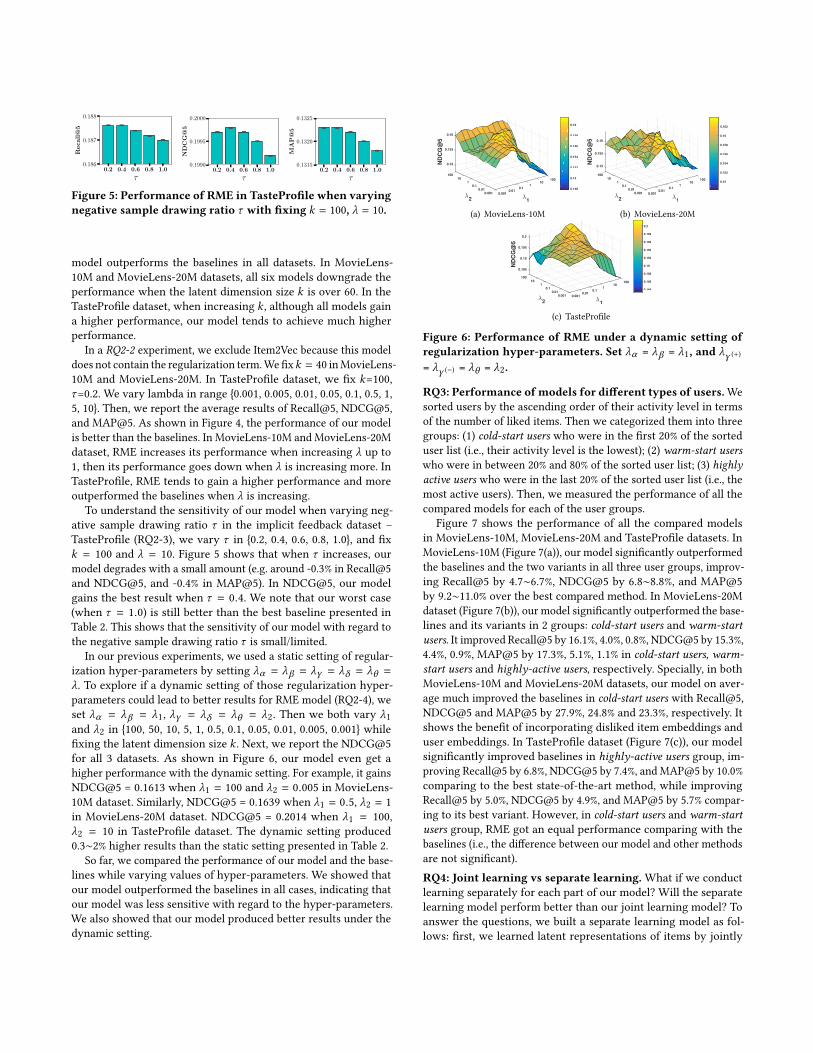
In our previous experiments, we used a static setting of regular-ization hyper-parameters by setting λα = λβ = λγ = λδ = λθ =λ. To explore if a dynamic setting of those regularization hyper-parameters could lead to better results for RME model (RQ2-4), weset λα = λβ = λ1, λγ = λδ = λθ = λ2. Then we both vary λ1and λ2 in 100, 50, 10, 5, 1, 0.5, 0.1, 0.05, 0.01, 0.005, 0.001 whilefixing the latent dimension size k . Next, we report the NDCG@5for all 3 datasets. As shown in Figure 6, our model even get ahigher performance with the dynamic setting. For example, it gainsNDCG@5 = 0.1613 when λ1 = 100 and λ2 = 0.005 in MovieLens-10M dataset. Similarly, NDCG@5 = 0.1639 when λ1 = 0.5, λ2 = 1in MovieLens-20M dataset. NDCG@5 = 0.2014 when λ1 = 100,λ2 = 10 in TasteProfile dataset. The dynamic setting produced0.3∼2% higher results than the static setting presented in Table 2.

So far, we compared the performance of our model and the base-lines while varying values of hyper-parameters. We showed thatour model outperformed the baselines in all cases, indicating thatour model was less sensitive with regard to the hyper-parameters.We also showed that our model produced better results under thedynamic setting.

10010

1

61

0.10.01

0.0010.0010.01

0.1

62

110

0.15

0.16

0.155

100

ND

CG

@5

0.148

0.15

0.152

0.154

0.156

0.158

0.16

(a) MovieLens-10M

10010

1

61

0.10.01

0.0010.0010.01

0.1

62

110

0.15

0.16

0.155

100

ND

CG

@5

0.15

0.152

0.154

0.156

0.158

0.16

0.162

(b) MovieLens-20M

10010

1

61

0.10.01

0.0010.0010.01

0.1

62

110

0.2

0.195

0.19

0.185

100

ND

CG

@5

0.184

0.186

0.188

0.19

0.192

0.194

0.196

0.198

0.2

(c) TasteProfile

Figure 6: Performance of RME under a dynamic setting ofregularization hyper-parameters. Set λα = λβ = λ1, and λγ (+)

= λγ (−) = λθ = λ2.

RQ3: Performance of models for different types of users.Wesorted users by the ascending order of their activity level in termsof the number of liked items. Then we categorized them into threegroups: (1) cold-start users who were in the first 20% of the sorteduser list (i.e., their activity level is the lowest); (2) warm-start userswho were in between 20% and 80% of the sorted user list; (3) highlyactive users who were in the last 20% of the sorted user list (i.e., themost active users). Then, we measured the performance of all thecompared models for each of the user groups.

Figure 7 shows the performance of all the compared modelsin MovieLens-10M, MovieLens-20M and TasteProfile datasets. InMovieLens-10M (Figure 7(a)), our model significantly outperformedthe baselines and the two variants in all three user groups, improv-ing Recall@5 by 4.7∼6.7%, NDCG@5 by 6.8∼8.8%, and MAP@5by 9.2∼11.0% over the best compared method. In MovieLens-20Mdataset (Figure 7(b)), our model significantly outperformed the base-lines and its variants in 2 groups: cold-start users and warm-startusers. It improved Recall@5 by 16.1%, 4.0%, 0.8%, NDCG@5 by 15.3%,4.4%, 0.9%, MAP@5 by 17.3%, 5.1%, 1.1% in cold-start users, warm-start users and highly-active users, respectively. Specially, in bothMovieLens-10M and MovieLens-20M datasets, our model on aver-age much improved the baselines in cold-start users with Recall@5,NDCG@5 and MAP@5 by 27.9%, 24.8% and 23.3%, respectively. Itshows the benefit of incorporating disliked item embeddings anduser embeddings. In TasteProfile dataset (Figure 7(c)), our modelsignificantly improved baselines in highly-active users group, im-proving Recall@5 by 6.8%, NDCG@5 by 7.4%, and MAP@5 by 10.0%comparing to the best state-of-the-art method, while improvingRecall@5 by 5.0%, NDCG@5 by 4.9%, and MAP@5 by 5.7% compar-ing to its best variant. However, in cold-start users and warm-startusers group, RME got an equal performance comparing with thebaselines (i.e., the difference between our model and other methodsare not significant).RQ4: Joint learning vs separate learning. What if we conductlearning separately for each part of our model? Will the separatelearning model perform better than our joint learning model? Toanswer the questions, we built a separate learning model as fol-lows: first, we learned latent representations of items by jointly

Cold start(*) Warm start(*) Highly active(*)

user’s activeness types

0.0

0.1

0.2

0.3

Reca

ll@

5

Item2Vec

WMF

Cofactor

U RME

I RME

RME

Cold start(*) Warm start(*) Highly active(*)

user’s activeness types

0.0

0.1

0.2

0.3

ND

CG

@5

Item2Vec

WMF

Cofactor

U RME

I RME

RME

Cold start(*) Warm start(*) Highly active(*)

user’s activeness types

0.0

0.1

0.2

MA

P@

5

Item2Vec

WMF

Cofactor

U RME

I RME

RME

(a) Dataset: MovieLens-10M. RME outperformed baselines in all three groups (p-value < 0.05).

Cold start(*) Warm start(*)Highly active(ns)

user’s activeness types

0.0

0.1

0.2

0.3

Reca

ll@

5

Item2Vec

WMF

Cofactor

U RME

I RME

RME

Cold start(*) Warm start(*)Highly active(ns)

user’s activeness types

0.0

0.1

0.2

0.3

ND

CG

@5

Item2Vec

WMF

Cofactor

U RME

I RME

RME

Cold start(*) Warm start(*)Highly active(ns)

user’s activeness types

0.00

0.05

0.10

0.15

0.20

MA

P@

5

Item2Vec

WMF

Cofactor

U RME

I RME

RME

(b) Dataset: MovieLens-20M. RME outperformed baselines in cold-start and highly-active user groups (p-value < 0.05).

Cold start(ns) Warm start(ns)Highly active(*)

user’s activeness types

0.0

0.1

0.2

Reca

ll@

5

Item2Vec

WMF

Cofactor

U RME

I RME

RME

Cold start(ns) Warm start(ns)Highly active(*)

user’s activeness types

0.0

0.1

0.2

ND

CG

@5

Item2Vec

WMF

Cofactor

U RME

I RME

RME

Cold start(ns) Warm start(ns)Highly active(*)

user’s activeness types

0.00

0.05

0.10

0.15

MA

P@

5

Item2Vec

WMF

Cofactor

U RME

I RME

RME

(c) Dataset: TasteProfile. RME outperformed baselines in highly-active user group (p-value < 0.05).

Figure 7: Performance of models for three user groups. Non-directional two-sample t-test was performed. * indicates signifi-cant (p-value < 0.05), and ns indicates not significant. The error bars are the average of standard errors in the 5 folds.

decomposing two SPPMI matrices X (+) and X (−) of liked item-itemco-occurrences and disliked item-item co-occurrences, respectively.Then, we learned user’s latent representations by minimizing theobjective function in Equation (4), where the latent representationsof items and item contexts were already learned and fixed. Next,we compared our joint learning model (i.e., RME) with the separatelearning model in MovieLens-10M, MovieLens-20M, and TastePro-file datasets. Our experimental results show that our joint learningmodel outperformed the separate learning model by significantlyimproving Recall@5, NDCG@5 and MAP@5 at least 12.1%, 13.5%and 17.1%, respectively (p-value < 0.001).

6 RELATEDWORKLatent factor models (LFM): Some of the first works in recom-mendation focused on explicit feedback datasets (name some: [15,30, 31]). Our proposed method worked well for both explicit andimplicit feedback settings with almost equal performances.

In implicit feedback datasets, which have been trending recentlydue to the difficulty of collecting users’ explicit feedback, properlytreating/modeling missing data is a difficult problem [4, 21, 27].Even though missing values are a mixture of negative feedback andunknown feedback, many works treated all missing data as nega-tive instances [8, 14, 27, 34], or sampled missing data as negativeinstances with uniform weights [28]. This is suboptimal becausetreating negative instances and missing data differently can fur-ther improve recommenders’ performance [13]. [25] proposed a

bagging of ALS learners [14] to sample negative instances. He et al.[13] assumed that unobserved popular items have a higher chanceof being negative instances. In our work, we attempted to non-uniformly sample negative instances in implicit feedback datasetsand treated them as additional information to enhance our modelperformance. Specifically, we (i) designed an EM-like algorithmwith a softmax function to draw personalized negative instancesfor each user; (ii) employed a word embedding technique to exploitthe co-occurrence patterns among disliked items, further enrichingtheir latent representations.LFM with auxiliary information: In latent factor models, addi-tional sources of information were incorporated to improve col-laborative filter-based recommender systems (e.g., user reviews,item categories, and article information [2, 10, 23, 35]). However,we only used an user-item-preference matrix without requiringadditional side information. Adding the side information into ourmodel would potentially further improve its performance. But, it isnot a scope of our work in this paper.LFM with item embeddings: [36] incorporated message embed-ding for retweet prediction. Cao et al. [6] co-factorized the user-item interaction matrix, user-list interaction matrix, and item-listco-occurrences to recommend songs and lists of songs for users.[20] learned liked item embeddings with an equivalent matrix fac-torization method of skip-gram negative sampling (SGNS), andperformed joint learning with matrix factorization. [3] exploiteditem embeddings using the SGNS method for item collaborative

filtering. So far, the closest techniques to ours [3, 20] only con-sidered liked item embeddings, but we proposed a joint learningmodel that not only considered LFM using matrix factorizationwith liked item embeddings, but also user embeddings and dislikeditem embeddings. Since integrating co-disliked item embeddingis non-trivial for implicit feedback datasets, we also proposed anEM-like algorithm for extracting personalized negative instancesfor each user.Word embeddings: Word embedding models [24, 26] representeach word as a vector of real numbers called word embeddings.In [19], the authors proposed an implicit matrix factorization thatwas equivalent to word2vec [24]. To extend word2vec, researchersproposed models that mapped paragraphs or documents to vectors[9, 18]. In our work, we applied word embedding techniques tolearn latent representations of users and items.

7 CONCLUSIONIn this paper, we proposed to exploit different co-occurrence in-formation: co-disliked item-item co-occurrences and user-user co-occurrences, which were extracted from the user-item interactionmatrix. We proposed a joint model combining WMF, co-liked em-bedding, co-disliked embedding and user embedding, following therecent success of word embedding techniques. Through compre-hensive experiments, we successfully demonstrated that our modeloutperformed all baselines, significantly improving NDCG@20 by5.6% in MovieLens-10M dataset, by 5.3% in MovieLens-20M dataset,and by 4.3% in TasteProfile dataset.We also analyzed how ourmodelworked on different types of users in terms of their interaction ac-tivity levels. We observed that our model significantly improvedNDCG@5 by 20.2% in MovieLens-10M, by 29.4% in MovieLens-20Mfor the cold-start users group. In the future extension of our model,we are interested in selecting contexts for users/items by setting atimestamp-based window size for timestamped datasets. In addi-tion, we are also interested in incorporating co-disliked patternsamong users (i.e., co-disliked user embeddings) into our model.

8 ACKNOWLEDGMENTThis work was supported in part by NSF grants CNS-1755536, CNS-1422215, DGE-1663343, CNS-1742702, DGE-1820609, Google FacultyResearch Award, Microsoft Azure Research Award, and Nvidia GPUgrant. Any opinions, findings and conclusions or recommendationsexpressed in this material are the author(s) and do not necessarilyreflect those of the sponsors.

REFERENCES[1] Deepak Agarwal and Bee-Chung Chen. 2009. Regression-based latent factor

models. In SIGKDD. 19–28.[2] Amjad Almahairi, Kyle Kastner, Kyunghyun Cho, and Aaron Courville. 2015.

Learning distributed representations from reviews for collaborative filtering. InRecSys. 147–154.

[3] Oren Barkan and Noam Koenigstein. 2016. Item2vec: neural item embedding forcollaborative filtering. In MLSP Workshop. 1–6.

[4] Immanuel Bayer, Xiangnan He, Bhargav Kanagal, and Steffen Rendle. 2017. Ageneric coordinate descent framework for learning from implicit feedback. InWWW. 1341–1350.

[5] Marcel Blattner, Yi-Cheng Zhang, and Sergei Maslov. 2007. Exploring an opinionnetwork for taste prediction: An empirical study. Physica A: Statistical Mechanicsand its Applications (2007), 753–758.

[6] Da Cao, Liqiang Nie, Xiangnan He, Xiaochi Wei, Shunzhi Zhu, and Tat-SengChua. 2017. Embedding Factorization Models for Jointly Recommending Itemsand User Generated Lists. In SIGIR. 585–594.

[7] Mukund Deshpande and George Karypis. 2004. Item-based top-n recommenda-tion algorithms. TOIS (2004), 143–177.

[8] Robin Devooght, Nicolas Kourtellis, and Amin Mantrach. 2015. Dynamic matrixfactorization with priors on unknown values. In SIGKDD. 189–198.

[9] Nemanja Djuric, Hao Wu, Vladan Radosavljevic, Mihajlo Grbovic, and NarayanBhamidipati. 2015. Hierarchical neural language models for joint representationof streaming documents and their content. In WWW. 248–255.

[10] Elie Guàrdia-Sebaoun, Vincent Guigue, and Patrick Gallinari. 2015. Latent tra-jectory modeling: A light and efficient way to introduce time in recommendersystems. In RecSys. 281–284.

[11] Ruining He and Julian McAuley. 2016. Ups and downs: Modeling the visualevolution of fashion trends with one-class collaborative filtering. In WWW. 507–517.

[12] Xiangnan He, Lizi Liao, Hanwang Zhang, Liqiang Nie, Xia Hu, and Tat-SengChua. 2017. Neural collaborative filtering. In WWW. 173–182.

[13] Xiangnan He, Hanwang Zhang, Min-Yen Kan, and Tat-Seng Chua. 2016. Fastmatrix factorization for online recommendation with implicit feedback. In SIGIR.549–558.

[14] Yifan Hu, Yehuda Koren, and Chris Volinsky. 2008. Collaborative filtering forimplicit feedback datasets. In ICDM. 263–272.

[15] Yehuda Koren. 2008. Factorization meets the neighborhood: a multifacetedcollaborative filtering model. In SIGKDD. 426–434.

[16] Yehuda Koren. 2009. Collaborative filtering with temporal dynamics. In SIGKDD.447–456.

[17] Yehuda Koren, Robert Bell, and Chris Volinsky. 2009. Matrix factorization tech-niques for recommender systems. Computer (2009).

[18] Quoc Le and Tomas Mikolov. 2014. Distributed representations of sentences anddocuments. In ICML. 1188–1196.

[19] Omer Levy and Yoav Goldberg. 2014. Neural word embedding as implicit matrixfactorization. In NIPS. 2177–2185.

[20] Dawen Liang, Jaan Altosaar, Laurent Charlin, and David M Blei. 2016. Factor-ization meets the item embedding: Regularizing matrix factorization with itemco-occurrence. In RecSys. 59–66.

[21] Dawen Liang, Laurent Charlin, James McInerney, and David M Blei. 2016. Mod-eling user exposure in recommendation. In WWW. 951–961.

[22] Bing Liu, Wee Sun Lee, Philip S Yu, and Xiaoli Li. 2002. Partially supervisedclassification of text documents. In ICML. 387–394.

[23] Julian McAuley and Jure Leskovec. 2013. Hidden factors and hidden topics:understanding rating dimensions with review text. In RecSys. 165–172.

[24] Tomas Mikolov, Ilya Sutskever, Kai Chen, Greg S Corrado, and Jeff Dean. 2013.Distributed representations of words and phrases and their compositionality. InNIPS. 3111–3119.

[25] Rong Pan, Yunhong Zhou, Bin Cao, Nathan N Liu, Rajan Lukose, Martin Scholz,and Qiang Yang. 2008. One-class collaborative filtering. In ICDM. 502–511.

[26] Jeffrey Pennington, Richard Socher, and Christopher D Manning. 2014. Glove:Global vectors for word representation. In EMNLP. 1532–1543.

[27] István Pilászy, Dávid Zibriczky, and Domonkos Tikk. 2010. Fast als-based matrixfactorization for explicit and implicit feedback datasets. In RecSys. 71–78.

[28] Steffen Rendle, Christoph Freudenthaler, Zeno Gantner, and Lars Schmidt-Thieme.2009. BPR: Bayesian personalized ranking from implicit feedback. In UAI. 452–461.

[29] Paul Resnick, Neophytos Iacovou, Mitesh Suchak, Peter Bergstrom, and JohnRiedl. 1994. GroupLens: an open architecture for collaborative filtering of netnews.In CSCW. 175–186.

[30] Ruslan Salakhutdinov, Andriy Mnih, and Geoffrey Hinton. 2007. RestrictedBoltzmann machines for collaborative filtering. In ICML. 791–798.

[31] Badrul Sarwar, George Karypis, Joseph Konstan, and John Riedl. 2001. Item-basedcollaborative filtering recommendation algorithms. In WWW. 285–295.

[32] Harald Steck. 2010. Training and testing of recommender systems on data missingnot at random. In SIGKDD. 713–722.

[33] Xiaoyuan Su and TaghiM. Khoshgoftaar. 2009. A Survey of Collaborative FilteringTechniques. Adv. Artificial Intellegence (2009).

[34] Maksims Volkovs and Guang Wei Yu. 2015. Effective latent models for binaryfeedback in recommender systems. In SIGIR. 313–322.

[35] Chong Wang and David M Blei. 2011. Collaborative topic modeling for recom-mending scientific articles. In SIGKDD. 448–456.

[36] Can Wang, Qiudan Li, Lei Wang, and Daniel Dajun Zeng. 2017. Incorporatingmessage embedding into co-factor matrix factorization for retweeting prediction.In IJCNN. 1265–1272.

[37] Hsiang-Fu Yu, Cho-Jui Hsieh, Si Si, and Inderjit S Dhillon. 2014. Parallel matrixfactorization for recommender systems. Knowledge and Information Systems(2014), 793–819.

[38] Weinan Zhang, Tianqi Chen, Jun Wang, and Yong Yu. 2013. Optimizing top-ncollaborative filtering via dynamic negative item sampling. In SIGIR. 785–788.

[39] Yunhong Zhou, Dennis Wilkinson, Robert Schreiber, and Rong Pan. 2008. Large-scale parallel collaborative filtering for the netflix prize. In International Confer-ence on Algorithmic Applications in Management. 337–348.