mathematics in finance - jan römanjanroman.dhis.org/finance/books notes thesises etc/math in...

Mathematics in Finance

Robert AlmgrenUniversity of Chicago

MAA Short CourseSan Antonio, TexasJanuary 11-12, 1999

2 Mathematics in Finance, Jan 11-12, 1999 Robert Almgren

Contents

1 Completeness and Arbitrage 51.1 One-period model . . . . . . . . . . . . . . . . . . . . . . . . . . . . . . 5

1.1.1 Future states . . . . . . . . . . . . . . . . . . . . . . . . . . . . . 51.1.2 Endowment and consumption . . . . . . . . . . . . . . . . . . 71.1.3 Securities and markets . . . . . . . . . . . . . . . . . . . . . . . 91.1.4 Arbitrage and pricing measures . . . . . . . . . . . . . . . . . 121.1.5 Risk-neutral pricing . . . . . . . . . . . . . . . . . . . . . . . . . 151.1.6 Valuing a single derivative . . . . . . . . . . . . . . . . . . . . . 16

1.2 Binomial trees . . . . . . . . . . . . . . . . . . . . . . . . . . . . . . . . 201.2.1 Stock price model . . . . . . . . . . . . . . . . . . . . . . . . . . 211.2.2 Pricing a derivative . . . . . . . . . . . . . . . . . . . . . . . . . 221.2.3 Dynamic hedging . . . . . . . . . . . . . . . . . . . . . . . . . . 231.2.4 Recombining trees . . . . . . . . . . . . . . . . . . . . . . . . . . 24

2 Real Market Securities 252.1 The basic assets . . . . . . . . . . . . . . . . . . . . . . . . . . . . . . . 25

2.1.1 Stocks . . . . . . . . . . . . . . . . . . . . . . . . . . . . . . . . . 252.1.2 Bonds and interest rates . . . . . . . . . . . . . . . . . . . . . . 262.1.3 Foreign exchange . . . . . . . . . . . . . . . . . . . . . . . . . . 27

2.2 Derivatives . . . . . . . . . . . . . . . . . . . . . . . . . . . . . . . . . . 272.2.1 Forwards and futures . . . . . . . . . . . . . . . . . . . . . . . . 272.2.2 Options . . . . . . . . . . . . . . . . . . . . . . . . . . . . . . . . 29

3 The Black-Scholes Equation 353.1 Refining the tree . . . . . . . . . . . . . . . . . . . . . . . . . . . . . . . 353.2 Continuum limit . . . . . . . . . . . . . . . . . . . . . . . . . . . . . . . 383.3 Solution of the Black-Scholes equation . . . . . . . . . . . . . . . . . 423.4 Dynamic hedging . . . . . . . . . . . . . . . . . . . . . . . . . . . . . . 443.5 American options . . . . . . . . . . . . . . . . . . . . . . . . . . . . . . 45

4 Stochastic Models 47

3

Chapter 1

Completeness and Arbitrage

Let’s begin with some of the main ideas and methods of mathematical fi-nance. These may seem a little abstract at first, but the ideas of arbitrage(more often, of its absence) and of a complete market underly everythingelse. The existence of these simple models and solutions has a stronginfluence on what kinds of models we are willing to make of the messyreal world, so I would rather get these ideas on the table first, before westart talking about real stocks, bonds, and options.

1.1 One-period model

In the first model we shall consider, there are two times. There is now,t = 0, at which we know everything about the world. There is a futuretime t = T , at which we do not know exactly what will happen. Wemake investment decisions now which will, in general, lead to uncertainoutcomes at time T .

1.1.1 Future states

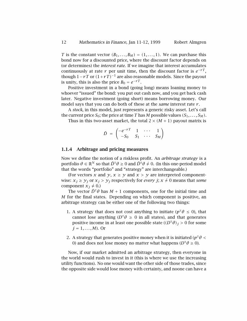
The classic theory relies on the following formulation: We make a list ofthe possible future states of the world. It is important for this theorythat this list is finite; if the number of possible future states is M , thenwe can just label states by numbers 1 to M . Let us call the set of statesΩ = 1, . . . ,M.

Here are some examples:

• A coin flip has two states: heads or tails. A lottery ticket either winsone of a few specified payoffs or nothing.

5


t

M

3

2

1

o

t = Tt = 0

Figure 1.1: M states at future time t = T .

• Either the Republican or the Democratic candidate will win electionin my district.

• If I am buying earthquake insurance, then I distinguish two states:either there is an earthquake (between now and time T , the expira-tion date of my policy) that knocks my house down, or there is not.Of course, the insurance company and I have to agree on what con-stitutes an insurable event. Actually, the policy might also coverpartial damage, so the number of states may be greater than two,but the two-state model might be a reasonable one to start with.

• Weather: I could measure the number of heating-degree days in aspecific month, and divide it into bins to make the state space finite.Oil prices move up and down.

• Most relevantly for our purposes, we might construct a model forthe price of a specified stock, in which at a specified future time,the price can take only one of a few finite values. Since stock pricesvary nearly continuously, this would clearly be an approximation,but it will turn out to be a useful one. Here the “event” is simplythe motion of the price itself; we are not claiming that it dependson any particular outside influence.

One thing we are explicitly not going to include in the theory at this pointis any opinion about the probability with which these different events willoccur. All we need is a finite list of possible events. (As Mr. Spock oncesaid, “This is not about probabilities, Lieutenant. We must be logical.”)

Robert Almgren Mathematics in Finance, Jan 11-12, 1999 7

It might be more accurate to say that we care only whether probabil-ities are zero or nonzero, but we don’t care what their values are. Weimplicitly assign zero probability to all events that are not in our list Ω(the coin might land on its edge).

A random variable is a functionΩ → R (real numbers). In other words,it is a vector (f (1), . . . , f (M)), where f(j) is the value this variable willtake if state j happens. A random variable can be represented as a (row)vector in the Euclidean space RM .

1.1.2 Endowment and consumption

In economics jargon, we measure our wealth in terms of a rather abstractquantity called a consumption good. In classical theory, consumptionis not the same as money; money is a social invention, which is usefulinsofar as it can be exchanged for the consumption good.

For example, if I acquire a lot of money, I can buy a Porsche. Myconsumption is not the car itself, but the experience of driving aroundin it, cornering as if on rails and receiving the envy of my neighbors. It ismy decision whether the consumption I sacrificed to achieve this state,for example, the time I spent working in the office, is worth the result.

For our purposes, we can equate consumption with money. That is,we are considering only a restricted set of the possible measures of suc-cess. For an individual, it might well be the case that applying thesetheories is more trouble that it is worth, indicating that important con-sumption quantities have been left out of the model. For large financialinstitutions, the relative cost is much less.

The reason we are given anything to consume is that we are given anendowment ; in our model, this is an amount of money we receive fromsome outside source depending on time and on the state of the world.Let us consider the endowmwent in the examples above:

• A coin flip does not in itself give me or cost me any money. (Ican enter into a contract with someone else, the value of whichdepends on the result of the flip.) A lottery ticket is similar: I haveno exposure unless I choose to buy it.

• It is possible that I will have financial exposure to the outcome ofan election. Perhaps I expect that a Republican win will drive thestock market upwards or downwards. Perhaps I expect a cushy jobin a Democratic administration.


• I spend money to buy or build a house. If no earthquake happensI keep the house so I have no new endowment. If an earthquakeknocks it down, then I have a huge negative endowment.

• Energy companies do have financial exposure to monthly averagetemperature, since consumption and consequently price depend onit. Airlines have huge exposure to oil prices, since they must buylarge quantites.

• The stock motion is like the coin flip: all kinds of stocks go up anddown all the time without concerning me. The only way I wouldhave exposure to the future stock motion is if at t = 0 I decide topurchase some shares, but this is not considered an endowment inthe classical sense.

Our future endowment is a random variable, which is not under ourcontrol. Our future consumption is also a random variable. Total endow-ment can be represented as the (M + 1)-vector (e0, e), where the scalare0 is the endowment at the initial time, and e is the M-vector (randomvariable) representing endowment at the final time. Similarly, total con-sumption can be represented (c0, c).

The purpose of financial markets is to provide mechanisms for mak-ing consumption different from endowment. For example,

• I can choose to bet on a coin flip, or to buy a lottery ticket. If I do,my consumption becomes very non-uniform.

• If I buy an insurance contract, I make my net consumption muchless random (I pay a small amount whatever happens, but I amguaranteed to still have a place to live).

• Energy companies buy and sell contracts whose value depends ontemperature, in order to eliminate the risk they are already exposedto. Airlines buy futures and options on fuel, to reduce or eliminatetheir risk.

• I may choose to buy a stock: in this case I generally am hoping thatthe price will rise and my consumption will, on average, be higherthan if I had not bought.

Another favorite economics concept is the utility function, which mea-sures the net value to me of a random consumption variable. This may


be represented as a function U(x) from RM to R; that is, it depends onthe entire spectrum of possible outcomes.

For example, when I decide to purchase earthquake insurance, I amjudging that my utility function is controlled by the worst possible out-come. Thus I am happy to protect myself against a downside risk, even ifstatistically (assigning probabilities to the events) my average gain is neg-ative. Fortunately, the insurance company has a different utility function(and different endowment), so the trade is mutually beneficial.

Utility functions are generally increasing, meaning that more is alwaysbetter, and concave, modeling to aversion to risk. Thus, if I have madea million dollars, I would still like to make more, but the second millionwill change my life less than did the first.

For our purposes, all we need to assume is that everyone in the markethas an increasing utility function. The reason is that we will be consider-ing the very special class of models and markets in which it is possible tocompletely eliminate risk. This is the theory that underlies the pricing offinancial derivatives such as options, and is the part that gives the mostclassical and cleanest mathematics. Needless to say, this is a very specialcategory, and very large and important areas of financial mathematics aredevoted to the modeling and management of risk.

1.1.3 Securities and markets

A security is a contract that pays different amounts in different states ofthe world; that is, it is a random variable d = (d(1), . . . , d(M)) ∈ RM .

For example, a bet on a coin flip would be represented as (1,−1). Anearthquake insurance contract might be represented as (0, P); it pays alarge amount P in the event of an earthquake. A stock might be repre-sented as, for example, (90,100,110), corresponding to the three possi-ble future prices.

We shall assume that every security can be purchased either long,meaning you hold a positive amount, or short, meaning that you hold anegative amount. That is, you can buy any real number θ of “shares,”and then your payout is the random variable (θd(1), . . . , θd(M)). Youcontrol this outcome by selecting θ at t = 0.

Thus you can choose either heads or tails on a coin flip. You caneither buy an insurance contract, or write one to your neighbor. You canbuy a stock, or “short” it, meaning that you borrow shares, sell them, andare obliged to purchase back the shares at a later date; you make moneyif the price has dropped in the meantime. Clearly the assumption of free


long or short investment is not sensible for every security, but for themain ones traded in financial markets it is reasonably good.

A market is a list of securities d1, . . . , dN . The market may be repre-sented by its N ×M payout matrix

D =

d1(1) · · · d1(M)

......

dN(1) · · · dN(M)

giving the amount that each security pays in each state of the world. Thenumber of securities N may be larger than, smaller than, or equal to thenumber of possible states M .

A portfolio is a list of investments

θ =

θ1...θN

where θj is the amount of security j you purchase at t = 0. The netpayout yielded by portfolio theta is the matrix product DTθ, where T de-notes transpose. The important point is that you must determine yourinvestment θ before the state is revealed. Thus the net payout is a ran-dom variable. Choosing the portfolio is your means for controlling yourconsumption in the presence of uncertain endowment.

The prices of the securities are given by the N-vector

p =

p1...pN

where pj is the money you have to invest to acquire one unit of securityj. Thus the total cost of portfolio θ is the scalar pTθ; this is not a randomvariable since p is known at the initial time.

For a given portfolio θ, your total consumption, meaning the amountof money you extract from the investment, is the (M+1)-vector (e0, e)+DTθ, where the N × (M + 1) augmented matrix

D =(−p D

)=

−p1 d1(1) · · · d1(M)

......

...−pN dN(1) · · · dN(M)


contains prices and payouts together. This matrix completely describesthe market. When these prices and payouts are posted, you are free tobuy or sell as much of each security as you would like, in order to tailoryour final consumption however you would like.

So far we have said nothing about how these prices are determined;they are offered to us and to every other participant by some mysteriousmarketplace “out there.” The entire point of this course is that the simpleprinciple of “no free lunch” (nonexistence of arbitrage, as defined below)imposes certain constraints on the prices. In particular,

1. We can write inequality conditions that must be satisfied by thecurrent prices in terms of their final payouts (the lesser point).

2. Most importantly: If our market is “complete” (see below), thenwhen we add a new security into the market, we can determine ex-actly what its price must be in terms of the prices and payouts ofexisting securities. The classic example is option pricing: if some-one proposes a new contract whose value depends on the value ofsomething that already exists in the market, then, using suitablemathematical models, we can determine what the price of the op-tion must be.

That’s really all that classical financial mathematics consists of. Onceyou are clear on the basic idea, the things that make it interesting are,first, the mathematical mechanisms for carrying out this computation invarious complicated situations, second, the kind of models about the realworld this simple theory forces us to believe, and, third, how the simpletheories are not adequate and what we can do about it.

In some cases you may already have opinions about what the priceshould be in terms of the payout. For example, coin flips and lotteriesare canonical examples of problems to which probability theory can beapplied. You would have difficulty getting someone to pay you to bet ona fair coin; the price of lottery tickets isset by the state and you may havestron opinions about whether they are fair (but you may buy one anywayfrom time to time). Remember that this theory does not care at all aboutprobabilities except as they are zero or nonzero; it is really only basedon the nonexistence of guaranteed profit.

Let us now consider two specific kinds of securities, which will be ourbuilding blocks.

A bond is a riskless asset. We will define a unit amount of a bondto pay a unit amount in all states of the world. Thus its payout at time


T is the constant vector (B1, . . . , BM) = (1, . . . ,1). We can purchase thisbond now for a discounted price, where the discount factor depends on(or determines) the interest rate. If we imagine that interest accumulatescontinuously at rate r per unit time, then the discount factor is e−rT ,though 1−rT or (1+rT)−1 are also reasonable models. Since the payoutis unity, this is also the price B0 = e−rT .

Positive investment in a bond (going long) means loaning money towhoever “issued” the bond: you put out cash now, and you get back cashlater. Negative investment (going short) means borrowing money. Ourmodel says that you can do both of these at the same interest rate r .

A stock, in this model, just represents a generic risky asset. Let’s callthe current price S0; the price at time T hasM possible values (S1, . . . , SM).

Thus in this two-asset market, the total 2× (M + 1) payout matrix is

D =(−e−rT 1 · · · 1−S0 S1 · · · SM

)

1.1.4 Arbitrage and pricing measures

Now we define the notion of a riskless profit. An arbitrage strategy is aportfolio θ ∈ RN so that DTθ ≥ 0 and DTθ 6= 0. (In this one-period modelthat the words “portfolio” and “strategy” are interchangeable.)

(For vectors x and y , x ≥ y and x > y are interpreted component-wise: xj ≥ yj or xj > yj respectively for every j; x 6= 0 means that somecomponent xj 6= 0.)

The vector DTθ has M + 1 components, one for the initial time andM for the final states. Depending on which component is positive, anarbitrage strategy can be either one of the following two things:

1. A strategy that does not cost anything to initiate (pTθ ≤ 0), thatcannot lose anything (DTθ ≥ 0 in all states), and that generatespositive income in at least one possible state ((DTθ)j > 0 for somej = 1, . . . ,M). Or

2. A strategy that generates positive money when it is initiated (pTθ <0) and does not lose money no matter what happens (DTθ ≥ 0).

Now, if our market admitted an arbitrage strategy, then everyone inthe world would rush to invest in it (this is where we use the increasingutility functions). No one would want the other side of those trades, sincethe opposite side would lose money with certainty, and noone can have a


risk exposure for which that is a good thing. There would thus be a hugeunbalanced demand from the market participants. Although we have notsaid anything about how prices are adjusted, any reasonable mechanismfor making prices respond to demand would cause the prices to move sothat the arbitrage opportunity disappeared (in chemistry, this is calledLe Chatelier’s principle).

A market is in equilibrium when this unbalanced demand does notexist, so the listed prices represent actual values at which other partici-pants are willing to take the other sides of the trades. The fundamentalprinciple of our pricing methods is that

Arbitrage strategies cannot exist in equilibrium.

The principle of absence of arbitrage is closely related to the efficiency ofmarkets, and the ability to quickly pounce on any profit opportunities.1

Our next job is to see what this rather abstract statement implies forthe relationship between the prices and the payout functions. This isprovided by the

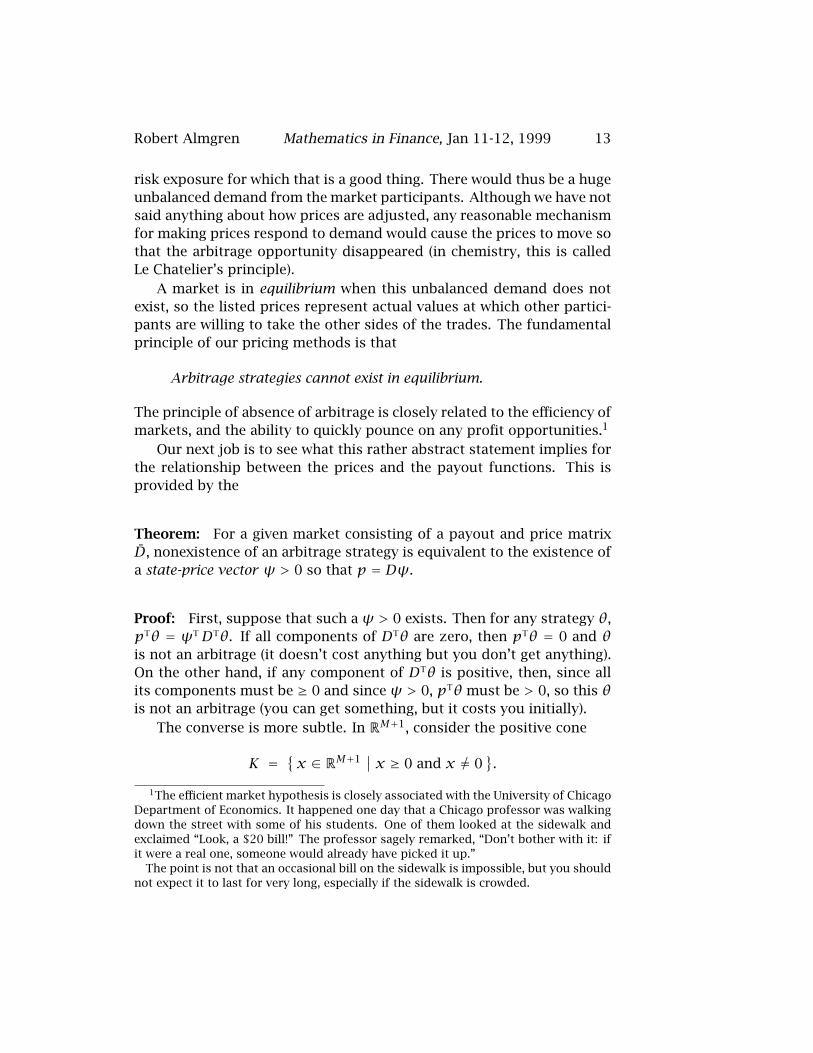
Theorem: For a given market consisting of a payout and price matrixD, nonexistence of an arbitrage strategy is equivalent to the existence ofa state-price vector ψ > 0 so that p = Dψ.

Proof: First, suppose that such a ψ > 0 exists. Then for any strategy θ,pTθ = ψTDTθ. If all components of DTθ are zero, then pTθ = 0 and θis not an arbitrage (it doesn’t cost anything but you don’t get anything).On the other hand, if any component of DTθ is positive, then, since allits components must be ≥ 0 and since ψ > 0, pTθ must be > 0, so this θis not an arbitrage (you can get something, but it costs you initially).

The converse is more subtle. In RM+1, consider the positive cone

K = x ∈ RM+1 ∣∣ x ≥ 0 and x 6= 0

.

1The efficient market hypothesis is closely associated with the University of ChicagoDepartment of Economics. It happened one day that a Chicago professor was walkingdown the street with some of his students. One of them looked at the sidewalk andexclaimed “Look, a $20 bill!” The professor sagely remarked, “Don’t bother with it: ifit were a real one, someone would already have picked it up.”

The point is not that an occasional bill on the sidewalk is impossible, but you shouldnot expect it to last for very long, especially if the sidewalk is crowded.


L

K

0

State 1

c

Figure 1.2: The arbitrage pricing theorem for N = 1, M = 1.

This is the set of payoffs (including initial cost) that constitute an arbi-trage. Also consider the linear subspace

L = x ∈ RM+1 ∣∣ x = DTθ for some θ ∈ RN .

This is the set of payoffs you can attain by some strategy; it has dimensionrank(D). An intersection of K and L would be an arbitrage; if there donot exist arbitrage strategies, then K and L are disjoint.

Now, both K and L are convex sets, and L is closed and linear. Thenthe separating hyperplane theorem says that there exists a linear functionF so that F(x) = 0 for all x ∈ L and F(y) > 0 for all y ∈ K.

By the Riesz representation theorem (trivial in finite dimensions), thelinear function can be represented as F(x) = cTx for some vector c ∈RM+1; c is a normal vector to L. We can write cTx = ax0+bTx, where x =(x0, x). Since K contains the positive coordinate axes, each componenta > 0, bj > 0. Returning to the definition of L, this means that for everyθ ∈ RN , −apTθ+bTDTθ = 0, or (ap−Db)Tθ = 0. Since ap−Db is just avector in RN , this can be true only if ap = Db, soψ = b/a is a state-pricevector.

The state-price vector assigns a positive weight ψj to each state j. Thetheorem says that if there is no arbitrage, then each initial price pi canbe computed by “collapsing” the payout vector (d(1), . . . , d(M)) againstψ, and we can use the same ψ for each security in our market. Note thatif rank(D) < M , then the state-price vector is not necessarily unique.


Theorem: A sufficient condition for the state-price vector to be uniqueis that rank(D) = M .

Proof: As noted, rank(D) is the dimension of the subspace L. If thisdimension is M , one less than the dimension of the space, then L has aunique normal vector c, the only candidate for the state-price vector.

Since D is an augmentation of D, rank(D) ≥ rank(D) and we have the

Corollary: A sufficient condition for the state-price vector to be uniqueis that rank(D) = M .

Since D is N ×M , its rank is at most the smaller of M and N . To haverank(D) = M , there must be at least N ≥ M securities in the market, andtheir payoffs must be independent vectors. A market with rank(D) = Mis called complete; in a complete market you can achieve any desiredcombination of payoffs in the different states, by suitable choice of in-vestment at the initial time.

Note that if there are more securities than states, so N > M , then itwould be possible for rank(D) to be ≥ M + 1. In this case, the subspaceL fills all of RM+1 and arbitrage is certainly possible.

If the number of possible future states is larger than the number ofindependent securities (in this one-period model) it is impossible for themarket to be complete. So the restriction to finitely many possible futurestates is essential in this model. In order to let the price take arbitrarilymany values, we shall also need to take many small time periods; it therelationship between the two continuum limits will set important restric-tions on the nature of our model.

1.1.5 Risk-neutral pricing

In order to interpret the significance of the components of ψ, let us sup-pose that one element in our market is a bond B with discount factorB0 = e−rT . The above representation says that B0 = B1ψ1 + · · ·BMψM =ψ1 + · · · +ψM . Thus if we define

q = erT ψ,

then each qj > 0 and their sum is one. We may thus interpret each qj asa “probability” that our model leads us to assign to state j; then absenceof arbitrage means that we can compute the price of any security in themarket by the formula

p = e−rT EQ[d] ≡ e−rT

(q1d(1)+ · · · + qMd(M)

).


Here the notation EQ means “expected value using the numbers q asprobabilities.” We are using the language of probability theory, but letus emphasize that the qj do not represent any sort of estimate of theprobability of anything happening in the real world. They are purelymathematical constructions; their values are forced on us by the rela-tionships between the prices and the payouts of the securities in themarket, and the assumption of nonexistence of arbitrage.

This result is so important and so fundamental that we will state itagain in words:

If the market does not admit arbitrage, then a purely artificialprobability measure can be constructed so that the price of anysecurity traded in the market is equal to the expectation of itsfuture value in that measure, discounted at the same rate asa risk-free bond. If the market is complete, this measure isunique.

This probability measure is often called the “risk-free measure.”

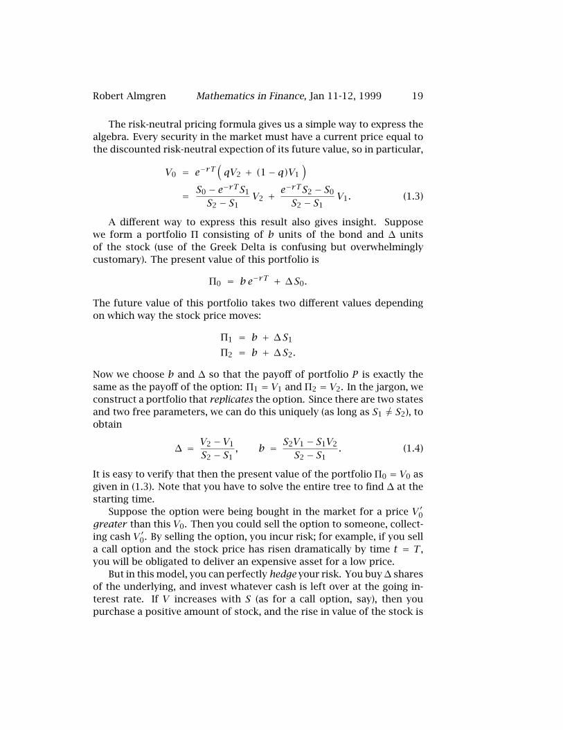
1.1.6 Valuing a single derivative

Let us now return to the simple model we have discussed above, in whichthe market consists of two assets. The first is a bond, with present valueB0 = e−rT and sure payoff 1 in every state. The second asset is a “stock”(it does not really matter what it is) with present value S0 and uncertainfuture value.

We shall suppose that only two future states are possible: the stockprice moves to value S1 or to value S2, with S1 < S2. We repeat that thesetwo states are not consequences of any external event in the world; theysimply represent our uncertainty about the future motion of the stockprice.

Now the augmented price matrix is

D =−e−rT −S0

1 S1

1 S2

in which the first column is the bond and the second column is the stock.The first row represents the initial time; the second and third rows arethe two possible future states.


1 - q

qS

t

exp(rT) S0

S1

S2

S0

t = Tt = 0

Figure 1.3: The 2-state stock motion model.

Since S1 6= S2, D has rank 2. Thus the linear set L in the arbitragetheorem is a plane. It has a unique normal vector (a, b1, b2), and so therisk-neutral measure is unique if it exists.

Denoting q1 = 1− q, q2 = q (Figure 1.3), we need only solve

S0 = e−rT(qS2 + (1− q)S1

)which gives

q = erTS0 − S1

S2 − S1, 1− q = S2 − erTS0

S2 − S1. (1.1)

These are the normalized state-price vector, as long as 0 < q < 1. Byinspection, this will be the case if

S1 < erTS0 < S2 (1.2)

This constraint is easily understood in direct financial terms.The theorem says that if (q,1−q) do not constitute a legitimate pric-

ing measure, then there exists an arbitrage portfolio. Suppose, for exam-ple, that erTS0 ≤ S1. Then do the following investment: At t = 0, borrowS0 cash, and use that money to purchase one share of stock, so you don’tinvest any of your own money. At t = T , you have to repay S0erT . Getthat money by selling the stock, which yields either S1 or S2. In the firstcase you definitely don’t lose, and in the second case you definitely makesomething since S2 > S1.


Conversely, if S1 < S2 ≤ erTS0 then interest rates are so high thatyou should short the stock and loan out the money. The only way thatneither of these strategies will not work is if the future stock value canbe either more or less than the amount earned by investing its currentvalue at the risk-free interest rate.

Now let’s make it interesting. Suppose our market contains a stock Sand a bond B, all of whose initial prices and possible payouts are specifiedso that there are no arbitrage possibilities. Now let’s add an additionalsecurity V into the market.

In general, if we add something else, we increase the number of states.For example, if we considered a second stock, then that stock could ingeneral move up or down independently of the first one, so we wouldhave at least four possible states in the extended model.

We will suppose that the new security is a derivative, meaning thatits value at the future time depends on the value of the underlying asset,in this case our original stock. There is an explicit function Λ(S), thepayout function, which gives the value of V in terms of the value of S attime T . Thus V1 = Λ(S1) and V2 = Λ(S2). The derivative security doesnot change its value independently of the underlying value (its value maydepend on other parameters such as the interest rate).

An example (we will discuss this more thoroughly in the next section)would be a call option with expiration date T . A call option gives you theright, but not the obligation, to purchase the asset at the specified datefor a prearranged value K, the strike price. If the asset is at that timetrading in the market for a price greater than K, you make a net profitS−K; if it is trading for a price less than K the option is worthless. ThusΛ(S) = maxS −K,0. (We are considering European options, which canbe exercised only on a single future date.)

We now have N = 3 securities but still M = 2 future states. The 3× 3augmented payout matrix is

D =−e−rT −S0 −V0

1 S1 V1

1 S2 V2

in which the only unknown quantity is V0.But we can immediately determine what V0 must be in terms of the

other prices in the problem. Recall that for nonexistence of arbitrageopportunities, we need rank(D) ≤ M . With M = 2, N = 3, D must bedegenerate.


The risk-neutral pricing formula gives us a simple way to express thealgebra. Every security in the market must have a current price equal tothe discounted risk-neutral expection of its future value, so in particular,

V0 = e−rT(qV2 + (1− q)V1

)

= S0 − e−rT S1

S2 − S1V2 + e−rT S2 − S0

S2 − S1V1. (1.3)

A different way to express this result also gives insight. Supposewe form a portfolio Π consisting of b units of the bond and ∆ unitsof the stock (use of the Greek Delta is confusing but overwhelminglycustomary). The present value of this portfolio is

Π0 = b e−rT + ∆S0.

The future value of this portfolio takes two different values dependingon which way the stock price moves:

Π1 = b + ∆S1

Π2 = b + ∆S2.

Now we choose b and ∆ so that the payoff of portfolio P is exactly thesame as the payoff of the option: Π1 = V1 and Π2 = V2. In the jargon, weconstruct a portfolio that replicates the option. Since there are two statesand two free parameters, we can do this uniquely (as long as S1 6= S2), toobtain

∆ = V2 − V1

S2 − S1, b = S2V1 − S1V2

S2 − S1. (1.4)

It is easy to verify that then the present value of the portfolio Π0 = V0 asgiven in (1.3). Note that you have to solve the entire tree to find ∆ at thestarting time.

Suppose the option were being bought in the market for a price V ′0greater than this V0. Then you could sell the option to someone, collect-ing cash V ′0. By selling the option, you incur risk; for example, if you sella call option and the stock price has risen dramatically by time t = T ,you will be obligated to deliver an expensive asset for a low price.

But in this model, you can perfectly hedge your risk. You buy∆ sharesof the underlying, and invest whatever cash is left over at the going in-terest rate. If V increases with S (as for a call option, say), then youpurchase a positive amount of stock, and the rise in value of the stock is


exactly enough to cover your increased liability. You incur no risk, andwalk away with a net profit. Because a lot of people will be trying to dothis if V ′0 > V0, the market price will be quickly driven down to V0. Thequantity ∆ is called the hedge ratio: the amount of stock you must holdper option you have sold to be risk-free.

This all sounds very clean and neat. But let’s review some of theassumptions that went into the model, and were essential for the results:

• You can buy or sell every asset in the market for the same price. Inreality, there are always transaction costs: brokerage fees, bid/askspreads, etc.

• You can buy arbitrary positive or negative amounts of every asset.In reality, short stock selling does not work exactly the same aslong purchasing: for example, there may be margin requirementson a short sale. Also, large transactions in the stock in order tocover options may move the stock price; we have assumed the stockmoves completely independently. There are other strange effects:for example, the Chicago options exchange closes 15 minutes afterthe New York exchanges on which the underlying stocks are traded,and this theory says nothing about the price an option should havewhen the stock is not freely tradeable.

• Most importantly, in a discrete-time model, you must specify thepossible values to which the price can move in the next time period.In the continuous-time limit, this corresponding to making a choicefor the volatility. But volatility does not have an unambiguous value,and different people have different opinions. In practice, choosingan option price is equivalent to choosing a value for the volatility.

1.2 Binomial trees

The above model can be extended to multiple periods. For simplicity, weshall consider the model of the last section, containing only a bond, astock, and eventually a derivative asset depending on the stock.

Let us suppose that time T is still the final horizon of our model, butlet us now divide that time into N sub-times t0, t1, . . . , tN , with t0 = 0(now) and tN = T . (Note: from now on, we shall no longer use N todenote the number of assets.)


S

t

S4,1

S4,2

S4,3

S4,12S4,15

S4,16

S21

S22

S23

S24

S11

S12

t3t2t1

S0

t 0 t4

Figure 1.4: A non-recombining tree with N = 4 time levels.

Let us suppose that the interest rate is constant. If the bond has afinal price BN = 1 at t = T , then at t = tj it will have price Bj = e−r(T−tj),independently of what the stock does.

1.2.1 Stock price model

At t = t0 (now), the stock price has a single known value S0 = S00, thatwe obtain by calling our broker. Let us suppose that in the first timeinterval, between t = t0 and t = t1, the stock may move to either of twopossible values, S11 or S12. Here, the first subscript denotes time levels,the second one denotes possible price values.

We further suppose that starting from the value at t1, there are exactlytwo new possible prices for each of the two price motions taken in thefirst period. There are thus four possible values the price can take at timet2, and each one corresponds to a sequence of two successive motions.Thus after two periods have elapsed, one of four possible things will havehappened; one of the following four trajectories will have occured:

S0 → S12 → S24

S0 → S12 → S23

S0 → S11 → S22

S0 → S11 → S21

As time increases, each state splits into two states. At the end of N


periods, there are therefore 2N possible states of the world. Each ofthese contains not only by a price SN,j , for j = 1, . . . ,2N , but also by theentire history that led to that price. Such a model, with two branches ateach node, is called a binomial tree (Figure 1.4).

For absence of arbitrage in this model, we need the prices on each“leaf” of the tree to satisfy the inequality constraint (1.2). Since the “chil-dren” of node (i, j) are (i + 1,2j − 1) and (i + 1,2j), we must apply itwith the substitutions

S0 , Si,j, S1 , Si+1,2j−1, S2 , Si+1,2j, T , ti+1 − ti

If this constraint were not satisfied at node (i, j), then we could con-struct an arbitrage strategy as follows: Do nothing until time ti. If thestock price has moved to Si,j , then carry out the arbitrage strategy at thattime. That strategy generates a guaranteed profit by time ti+1. It is notguaranteed that the price will reach Si,j , but that event is possible, andhence this is an arbitrage strategy at the initial time.

1.2.2 Pricing a derivative

Here again, it gets interesting when we add an additional security. Sup-pose we add an option V . Suppose that the value of V is explicitly knownat time tN in terms of the price of S at that time. For example, V is acall option for which tN is exactly the “exercise date,” the time at whichit can be exercised. Thus we know the values VN,j for each j.

Now we claim that we can use the pricing formula (1.3) to work back-wards on the tree, all the way back to the current time t0 and currentstock price S0. We first use the formula to determine the values VN−1,∗at the next-to-last level in terms of the final values VN,∗. Then we deter-mine the values VN−2,∗ in terms of the VN−1,∗. We repeat until we are leftwith the single number V0, which is the price the option “ought” to betrading at in the market right now. By introducing multiple intermediatetimes at which trading is possible, we have been able to let the stock pricetake more than two values at the final time.

The reason this should be satisfied is as described above. If at anynode on the tree this algebraic relation were not satisfied, then by waitingto see if the stock price actually moved to that node, we would have afinite chance of making a profit, with no chance of loss. And, providedV is fully known at t = T , the algebraic relations are enough to fix V0.


1.2.3 Dynamic hedging

Along with the derivative value V , this algebra also gives us various aux-iliary quantities at each node. Of these, the risk-neutral weight q has nodirect meaning; we emphasize that it is not the probability of anythingreally happening in the world.

But the hedge ratios∆i,j are the key to the whole pricing strategy. Thereason that the price of the option is uniquely defined at t = 0 is thatthere exists a dynamic hedging strategy that replicates its value at thefinal time. Thus the value of the option must be exactly equal to the costof implementing the hedging strategy, or else there would be arbitrageopportunities.

In words, the strategy is the following. Suppose you sell an option tosomeone at time t = 0 for price V0. At the same time, you go out andpurchase∆0 shares of the stock; you deposit or borrow any left-over cashinto or from an interest-bearing account.

At time t1, the stock price will have moved either to S1,1 or to S1,2.Depending on which it has done, you adjust your stock position to ∆1,1or to ∆1,2. This may yield some cash (if the new ∆ is smaller than theold one) or require an input of cash. In either case you give or take tothe interest-bearing account. In no case do you ever bring in cash fromoutside.

As time evolves and the stock price moves up and down, you continuethis juggling act, continually rebalancing your position. At the final time,you will have exactly the right amount of stock and cash to cover yourobligation to the person who bought the option, and you will be back tozero. (In practice, you add a markup to the initial option price to makeyourself a sure profit.)

This strategy was invented in 1973 by Black, Scholes, and Merton; itis what they got the Nobel prize for (in the continuous-time limit).

Note that you have to continually adjust your stock holdings as thestock price changes. We can therefore add another to our list of keyassumptions that go into the Black-Scholes pricing theory:

• You can rebalance your portfolio as frequently as prices move. Sinceprices generally move extremely rapidly, it is impractical to carryout this strategy exactly as described. Imperfect hedging leads tononvanishing risk associated with writing an option.

Despite the immense simplifications that go into it, the Black-Scholesstrategy has a tremendous importance. It brings the problem of deter-


S

t

S0

S41

S 42

S43

S44

S45

S31

S32

S33

S 34

S21

S22

S23

S11

S12

t4t 0 t1 t2 t3

Figure 1.5: A recombining tree with N = 4 time levels.

mining an option price down from the realm of speculation, into theframework of something you can study rationally if imperfectly.

1.2.4 Recombining trees

One final wrinkle needs to be added. As you may already have observedand been wondering about, a tree as described above and as pictured inFigure 1.4 is extremely impractical. With N time levels, it has 2N nodesat the final time. If N is large enough to achieve a reasonable degreeof time resolution, this is an astronomical number. Furthermore, thesevalues overlap in a horrendous way.

For practical purposes (both numerical and analytical computation)it is more reasonable to require the tree to be recombining as shown inFigure 1.5. In such a tree, we require an up motion followed by a downmotion to give the same price as a down motion followed by an up motion.

A recombining tree has onlyO(N2) elements forN time levels, so it ispossible to achieve reasonable refinement in both time and stock price.By constructing this tree, we are assuming that the stock price will jumpup and down on a grid whose structure we know in advance.

Of course, it remains to be seen what any of this really means. We canassume whatever we like about the future motion of a financial asset, butthe world and the marketplace are under no obligation to conform to ourmodel. We need a reasonable characterization of exactly what featuresof the tree determine the final price that we compute (Chapter 3).

mathematics in finance - jan römanjanroman.dhis.org/finance/books notes thesises etc/math in...

Documents