materials modelling with castep - archer » – lda, gga (pw91, pbe, rpbe, blyp, wc,..) lsda and...

Materials modelling with CASTEP

Keith RefsonScience and Technology Facilities Council (RAL)

History and Prehistory

•Complete re-engineering of a new plane-wave code from scratch beginning 1999. (Original CASTEP code by Mike Payne/Accelrys reached end of life in 1990s.)

•Core “Developer Group” of P. Hasnip, S. Clark, M. Probert, C. Pickard, M. Segall, P. Lindan, (Payne) and in 2002, K. Refson and 2007, Jonathan Yates

•Commercialised by Accelrys and integrated into Materials Studio – flexible, easy to use GUI.

•Aim: build a flexible, well-engineered development platform for new physics using modular software practices and documented API specification.

•Parallel and HPC use built in from start.

•Release 1 in late 2001. Now at release 7.0.

•Comprehensive “Core” functionality with broad suite of capabilities for Structure, dynamics and spectroscopy.

Availability and Licenses

● Free of charge UK academic license through UK Car-Parrinello Consortium agreement. Forms and instructions at

http://ccpforge.cse.rl.ac.uk/projects/castep

N.B. Your research group must be licensed before access is granted to Archer version.

● European academic source code license €1800. Available

● from Accelrys inc. http://www.accelrys.com● Commercial version available worldwide through Materials Studio

prroduct, also from Accelrys inc. http://www.accelrys.com


http://www.accelrys.com/

Support and Resources

● Website: http://www.castep.org● Mailing list [email protected]. sign up at

http://www.jiscmail.org/CASTEP● UK developer/support/download site


http://www.castep.org/

mailto:[email protected]

http://www.jiscmail.org/CASTEP

CASTEP Training Workshop

● August 18-23, Oxford● Focus on NMR, Vibrational spectroscopy and AIRSS● Sponsored by CCP-NC. Fee £100● Application deadline 31 May 2014● http://www.castep.org/CASTEP/Workshop2014

Huge range of science

● Nanotechnology (CNT, QD)● Minerals and materials● High-pressure physics● Catalysis● Optical spectroscopy● Liquids and solutions● Molecular crystals● Battery and fuel cell materials● Surface physics/chemistry● Defects/colour centres

● NMR Crystallography● Ex-nihilo crystal structure

prediction● INS, IXS, spectroscopy● Optical spectroscopy● EELS● XAS● Dielectric materials

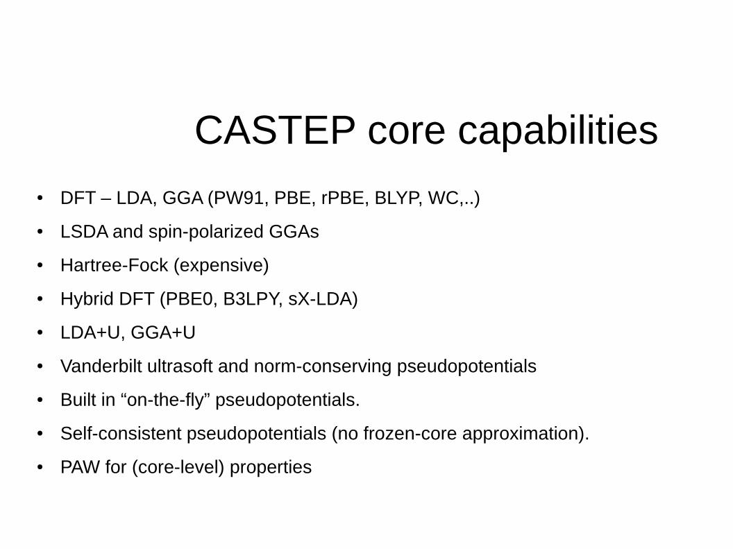
CASTEP core capabilities● DFT – LDA, GGA (PW91, PBE, rPBE, BLYP, WC,..)

● LSDA and spin-polarized GGAs

● Hartree-Fock (expensive)

● Hybrid DFT (PBE0, B3LPY, sX-LDA)

● LDA+U, GGA+U

● Vanderbilt ultrasoft and norm-conserving pseudopotentials

● Built in “on-the-fly” pseudopotentials.

● Self-consistent pseudopotentials (no frozen-core approximation).

● PAW for (core-level) properties

Structure and Dynamics in CASTEP

● Geometry optimization with Cartesian BFGS or internal co-ordinates.

● Standard (BFGS) or loe-memory (L-BFGS) variants.

● Variable cell geometry optimization under pressure.

● Molecular dynamics in NVE, NVT, NPH ensembles,

damped and langevin MD

● Path integral MD (PIMD) for nuclear quantum dynamics.

● Genetic algorithm structure searching

● LST/QST transition-state searching

● (L-BFGS, NEB and more under development)

CASTEP can perform wide variety of spectroscopic calculations

• IR and raman spectroscopy (vibrational/phonon)

• INS and IXS spectroscopy (vibrational phonon)

• Conduction-band optical dielectric spectra (EELS etc)

• Core level spectroscopy (ELNES, XANES)

• NMR chemical shifts

Spectroscopy in CASTEPSpectroscopy in CASTEP

CASTEP has a variety of Hamiltonians and XC functionals

• Pure local DFT (LDA,LSDA, PBE, RPBE, WC,...)

• Hybrid HF exchange methods (HF, Screened HF, PBE0, B3LYP

• Model methods (LDA+U)

• More under development.

Recent developments● DFT+D for dispersion forces (Tkatchenko/Scheffler and Grimme schemes)

● Finite-displacement phonons with hybrid functionals and LDA+U.

● L_BFGS for geometry optimisation of very large systems.

● Better adaptive parallelism.

● Band parallelism

● Optimised disk I/O for massively parallel case

● Optimised FFT parallelism for multicore clusters using system V shared memory

● Phonons for metallic systems using DFPT

● Electron localisation functions (ELF) and Hirshfeld charges

● Non-collinear magnetism

● Time-dependent DFT

Running CASTEP

Input and Output filesCASTEP I/O based on root name <seed> with suffixes

Input files

Output files

Input & Output files

<seed>.cell Input structure and structure-related quantities<seed>.param Parameters and options to control the calculation

<seed>.castep Main human-readable output file<seed>.bands Electronic eigenvalues from SCF, Bandstructure, DOS<seed>.orbitals Electronic eigenvectors from DOS/Bandstructure<seed>.den_fmt Formatted electron density for analysis or visualization<seed>.geom Formatted optimization trajectory<seed>.phonon Phonon eigenvectors and eigenvalues...

<seed>.check Binary checkpoint file, containing all orbitals<seed>.castep_bin Binary checkpoint file, without orbitals

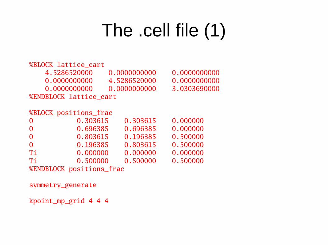
The .cell file (1)

%BLOCK lattice_cart 4.5286520000 0.0000000000 0.0000000000 0.0000000000 4.5286520000 0.0000000000 0.0000000000 0.0000000000 3.0303690000%ENDBLOCK lattice_cart

%BLOCK positions_fracO 0.303615 0.303615 0.000000O 0.696385 0.696385 0.000000O 0.803615 0.196385 0.500000O 0.196385 0.803615 0.500000Ti 0.000000 0.000000 0.000000Ti 0.500000 0.500000 0.500000%ENDBLOCK positions_frac

symmetry_generate

kpoint_mp_grid 4 4 4

The .cell file%BLOCK lattice_abc 4.528652 4.528652 3.030369 90.0 90.0 90.0%ENDBLOCK lattice_abc

%BLOCK positions_abs ang O 1.3749666 1.3749666 -0.0000000 O 3.1536853 3.1536853 0.0000000 O 3.6392926 0.8893593 1.5151845 O 0.8893593 3.6392926 1.5151845 Ti -0.0000000 -0.0000000 -0.0000000 Ti 2.2643260 2.2643260 1.5151845%ENDBLOCK positions_abs

kpoint_mp_spacing 0.05 1/bohr

Jmol can visualise .cell file directly: $ jmol tio2.cellUse to check your input!

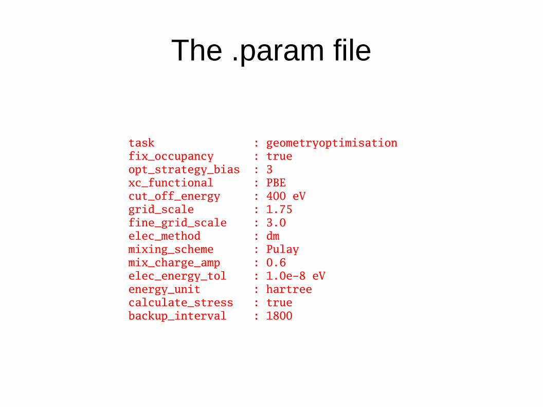
The .param file

task : geometryoptimisationfix_occupancy : trueopt_strategy_bias : 3xc_functional : PBEcut_off_energy : 400 eVgrid_scale : 1.75fine_grid_scale : 3.0elec_method : dmmixing_scheme : Pulaymix_charge_amp : 0.6elec_energy_tol : 1.0e-8 eVenergy_unit : hartreecalculate_stress : truebackup_interval : 1800

Some useful options

castep.serial --version

castep.serial –dryrun quartz

On Archer, after “module load castep.serial”

Read input files, check syntax generate pseudopotentials and exit

castep.serial –help search kpoint

castep.serial –help xc_functional

Print list of cell and param keywords matching “kpoint”

Print brief description of “xc_functional” keyword

Preparing Input Structures

● Crystal structures – eg from ICSD cif2cell

(http://sourceforge.net/projects/cif2cell/)

– Supports many codes in addition to CASTEP– Advanced options for supercell generation/alloys

● GUI (Commercial) Accelrys – Materials Studio

(http://www.accelrys.com/)● GUI (Free) aten (http://www.projectaten.org/)● GUI (Free) Avogadro (http://avogadro.cc/)

http://sourceforge.net/projects/cif2cell/

The .castep output file

Aims to be definitive record of run:

● Output optimised for human readability● Version of CASTEP used● Values of user-specified and default input parameters

- everything necessary to re-create at later date.● Progressive log of run details● SCF and geometry convergence progress● Final geometry● Phonon frequencies, spectroscopic information● Timing and memory information● Can be directly read by Jmol for visualisation

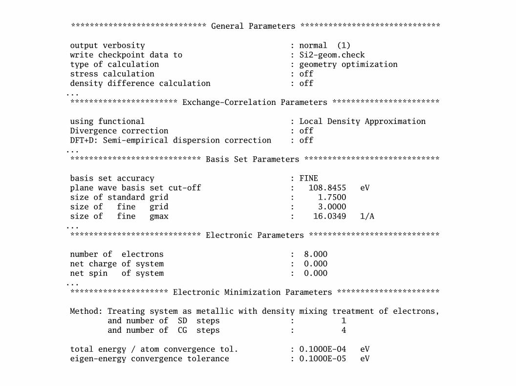
***************************** General Parameters ****************************** output verbosity : normal (1) write checkpoint data to : Si2-geom.check type of calculation : geometry optimization stress calculation : off density difference calculation : off... *********************** Exchange-Correlation Parameters *********************** using functional : Local Density Approximation Divergence correction : off DFT+D: Semi-empirical dispersion correction : off... **************************** Basis Set Parameters ***************************** basis set accuracy : FINE plane wave basis set cut-off : 108.8455 eV size of standard grid : 1.7500 size of fine grid : 3.0000 size of fine gmax : 16.0349 1/A... **************************** Electronic Parameters **************************** number of electrons : 8.000 net charge of system : 0.000 net spin of system : 0.000... ********************* Electronic Minimization Parameters ********************** Method: Treating system as metallic with density mixing treatment of electrons, and number of SD steps : 1 and number of CG steps : 4 total energy / atom convergence tol. : 0.1000E-04 eV eigen-energy convergence tolerance : 0.1000E-05 eV

+---------------- MEMORY AND SCRATCH DISK ESTIMATES PER PROCESS --------------+| Memory Disk || Model and support data 15.5 MB 2.3 MB || Electronic energy minimisation requirements 0.7 MB 0.1 MB || ----------------------------- || Approx. total storage required per process 16.2 MB 2.4 MB || || Requirements will fluctuate during execution and may exceed these estimates |+-----------------------------------------------------------------------------+Calculating finite basis set correction with 3 cut-off energies.Calculating total energy with cut-off of 98.846eV.------------------------------------------------------------------------ <-- SCFSCF loop Energy Fermi Energy gain Timer <-- SCF energy per atom (sec) <-- SCF------------------------------------------------------------------------ <-- SCFInitial -9.55691424E+000 0.00000000E+000 10.98 <-- SCF 1 -2.98642516E+002 8.50306978E+000 1.44542801E+002 11.13 <-- SCF 2 -3.22530892E+002 5.98069026E+000 1.19441881E+001 11.23 <-- SCF 3 -3.23350195E+002 5.58050764E+000 4.09651079E-001 11.31 <-- SCF 4 -3.23130108E+002 5.80496213E+000 -1.10043094E-001 11.47 <-- SCF 5 -3.23113582E+002 5.90225188E+000 -8.26313227E-003 11.64 <-- SCF 6 -3.23113840E+002 5.90677071E+000 1.28878855E-004 11.80 <-- SCF 7 -3.23113881E+002 5.91037067E+000 2.03552610E-005 11.95 <-- SCF 8 -3.23113881E+002 5.91039673E+000 5.85819903E-008 12.10 <-- SCF 9 -3.23113881E+002 5.91039217E+000 5.15119118E-009 12.25 <-- SCF------------------------------------------------------------------------ <-- SCF Final energy, E = -323.1138724516 eVFinal free energy (E-TS) = -323.1138806912 eV(energies not corrected for finite basis set) NB est. 0K energy (E-0.5TS) = -323.1138765714 eV

Checkpoint and Restart

In-run checkpointing enabled by parameter backup_interval 2600Or num_backup_iter 5Which will periodically write <seed>.check

Run can be continued by setting continuation : defaultOr continuation : <seed>.checkIn param file.

Allows continuations of geometry, MD, phonon calculations.

Bandstructure restart uses temporary mechanism and is Under revision.

Pseudopotentials

General remarks on pseudopotentials

Pseudopotentials have acquired some mystique – even seen as a “black art”

Not so – they are theoretically well-founded and rigorous, BUT● No easy physical picture as with atomistic potentials.● Ab initio nature hidden away● Too many different recipies for generating them● Transferrability and accuracy can be systematically improved,

but are not guaranteed by any procedure.● Known pitfalls such as “ghost states” can occur unpredictably.● Only trial-and-error generation testing can give accurate PSPs

Pseudopotential generation and testing requires expertise and patience – not for beginners.

On-the-fly (OTF) generation

Unique to CASTEP – built-in pseudopotential generation%BLOCK species_potSi 3|1.8|2|4|6|30:31:32O 2|1.0|1.3|0.7|13|16|18|20:21(qc=7)%ENDBLOCK species_pot

1. Explicit specification

2. Built-in library

1. Explicit specification

%BLOCK species_pot%ENDBLOCK species_pot

Cutoff defaults embedded in string. Select by param keyword basis_precision : coarse/medium/fineas alternative to cut_off_energy : 500 eV

Also need to choose size of second (fine) FFT grid for augmentation density in case of ultrasoft PPs.

Easiest way to choose is parameter fine_grid_scale : swith scale-factor s usually in range 2-4. Unfortunately no automatic default (yet).

Pseudopotential files and libraries

Can also specify pseudopotentials saved in files%BLOCK species_potSi Si_00.usp%ENDBLOCK species_pot

Recognised formats are<name>.usp - CASTEP's own format. Used for legacy USPP library and for saving OTF potentials. Can contain USPP or NC.<name>.recpot - Older format for norm-conserving (NC) only. Used for 1990S NC library and Opium-generated NC PSPs.<name>.upf - The Quantum Espresso universal format. (Not available until CASTEP 8.0)

Set environment variable PSPOT_DIR to search directory file PSP files – no need to copy these around.

$ export PSPOT_DIR=/usr/local/share/pseudopotentials

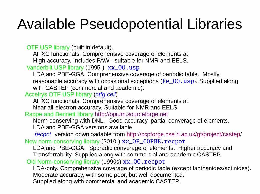
Available Pseudopotential Libraries

OTF USP library (built in default). All XC functionals. Comprehensive coverage of elements at High accuracy. Includes PAW - suitable for NMR and EELS. Vanderbilt USP library (1995-) xx_00.usp LDA and PBE-GGA. Comprehensive coverage of periodic table. Mostly reasonable accuracy with occasional exceptions (Fe_00.usp). Supplied along with CASTEP (commercial and academic). Accelrys OTF USP library (otfg.cell) All XC functionals. Comprehensive coverage of elements at Near all-electron accuracy. Suitable for NMR and EELS. Rappe and Bennett library http://opium.sourceforge.net Norm-conserving with DNL. Good accuracy. partial converage of elements. LDA and PBE-GGA versions available. .recpot version downloadable from http://ccpforge.cse.rl.ac.uk/gf/project/castep/ New norm-conserving library (2010-) xx_OP_00PBE.recpot LDA and PBE-GGA. Sporadic converage of elements. Higher accuracy and Transferrability. Supplied along with commercial and academic CASTEP. Old Norm-conserving library (1990s) xx_00.recpot LDA-only. Comprehensive coverage of periodic table (except lanthanides/actinides). Moderate accuracy, with some poor, but well documented. Supplied along with commercial and academic CASTEP.

Accuracy Benchmarks

a/A c/A u PW-LDA (OTF1) 4.550 (-0.18%) 2.919 (-0.03%) 0.3039 PW-LDA (OTF2)(SC) 4.549 (-0.20%) 2.919 (-0.03%) 0.3039 PW-LDA ( 00.usp) 4.551 (-0.15%) 2.921 (+0.03%) 0.3039 PW-LDA (VASP-PAW) 4.557 (-0.22%) 2.928 (+0.27%) 0.304

PW-LDA (Rappe-Bennett) 4.563 (+0.11%) 2.932 (+0.41%) 0.3040 PW-LDA (Old recpot) 4.596 (+0.84%) 2.984 (+2.19%) 0.3041 PW-LDA (New recpot) 4.526 (-0.70%) 2.908 (-0.41%) 0.3041 PW-LDA (TM) 4.536 (-0.48%) 2.915 (-0.17%) 0.304

FP-LAPW-LDA 4.558 2.920 0.3039 Expt 4.582 (+0.53%) 2.953 (+1.13%) 0.305

Crystal structure of rutile TiO2

Electronic SCF

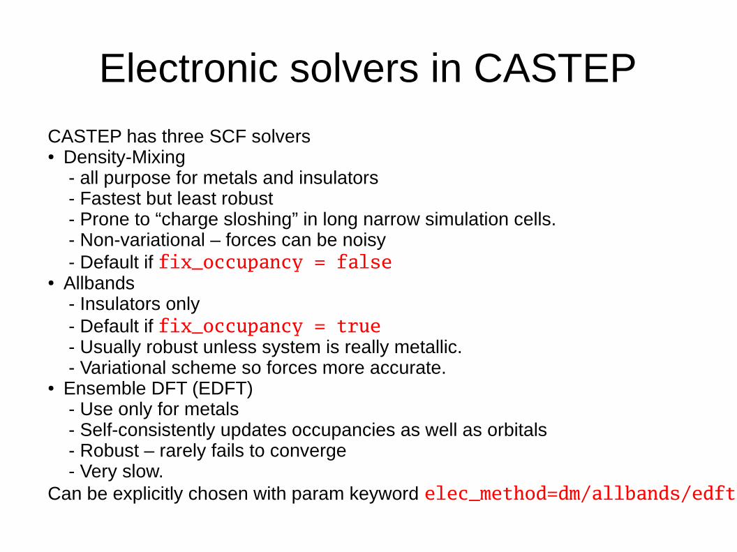
Electronic solvers in CASTEP

CASTEP has three SCF solvers● Density-Mixing

- all purpose for metals and insulators - Fastest but least robust - Prone to “charge sloshing” in long narrow simulation cells. - Non-variational – forces can be noisy - Default if fix_occupancy = false

● Allbands - Insulators only - Default if fix_occupancy = true - Usually robust unless system is really metallic. - Variational scheme so forces more accurate.

● Ensemble DFT (EDFT) - Use only for metals - Self-consistently updates occupancies as well as orbitals - Robust – rarely fails to converge - Very slow.

Can be explicitly chosen with param keyword elec_method=dm/allbands/edft

Metals and InsulatorsParam file keyword to allow/forbid metallic behaviour is fix_occupancy : true/false

Convergence failure or even false convergence possible if metallic systemTreated as fixed occupancy.

N.B. fix_occupancy : true changes default solver from DM to allbands.

Use eigenvalue smearing scheme to accelerate k-point convergence in a metal smearing_scheme : Gaussian/coldsmearing/... Additional parameter controls degree of broadening applied smearing_width : 0.2 eV

This is analogous to setting a high temperature for the electrons, and 0K resultsare only recovered in the w->0 limit.

Nonzero TS term in .castep output is sure sign of metallic occupancy. Final energy, E = -3158.505634320 eVFinal free energy (E-TS) = -3158.663886719 eV(energies not corrected for finite basis set) NB est. 0K energy (E-0.5TS) = -3158.584760519 eV

Magnetism

%BLOCK POSITIONS_FRAC O -0.25 -0.25 -0.25 O 0.25 0.25 0.25 Mn 0.00 0.00 0.00 SPIN= 2.0 Mn 0.50 0.50 0.50 SPIN= -2.0%ENDBLOCK POSITIONS_FRAC

Use SPIN= modifier in .cell file to specify initial spin state (DM solver only)

N.B. Sum of SPIN= .cell file must be consistent with spin= in .param.

After SCF converged the final spin state is reported in .castep (antiferromagnetic)

2*Integrated Spin Density = 0.150754E-07 2*Integrated |Spin Density| = 9.18570 Final energy, E = -6430.818475862 eV

2*Integrated Spin Density = 4.89553 2*Integrated |Spin Density| = 4.89568 Final energy, E = -3215.241900426 eV

Ferromagnetic

Spin-polarisation activated by param keywords spin=s or spin_polarised : true

SCF convergence failures

● Is there a mistake in the geometry violating the rules of chemical bonding?

● Are you treating as an insulator a system which is trying to be metallic.

● Are you treating a system trying to be magnetic as unpolarised?

● Have you broken the spin symmetry for a magnet?

● If using Broyden density mixing, try switching to Pulay and vice versa

● Try increasing mix_cut_off_energy, decreasing mixing parameters

● If all else fails, switch to EDFT

Symmetry

K

K'

CASTEP uses crystallographic symmetry for● SCF: Reduce memory and calculation by treating only part

of k-point set within irreducible Brillouin zone (IBZ)● Geometry: Constrain optimisation not to break symmetry● Phonons: Reducing q-point grids to IBZ and only calculating

Perturbations of inequivalent atoms.● Phonons: Symmetry analysis of vibrational modes.

Example: graphite – 6-fold reduction in size of k-point set needed

Using Symmetry in CASTEPStraightforward way is to use .cell file keywords SYMMETRY_GENERATE KPOINT_MP_GRID : p q rwhich automatically detects symmetry and generates reduced k-point mesh.

Alternatively, cif2cell and Materials Studio generate explicit symmetry operations in .cell:

%BLOCK symmetry_ops# Symm. op. 1 E 1.000000000000000 0.000000000000000 0.000000000000000 0.000000000000000 1.000000000000000 0.000000000000000 0.000000000000000 0.000000000000000 1.000000000000000 0.000000000000000 0.000000000000000 0.000000000000000# Symm. op. 2 I -1.000000000000000 0.000000000000000 0.000000000000000 0.000000000000000 -1.000000000000000 0.000000000000000 0.000000000000000 0.000000000000000 -1.000000000000000 0.000000000000000 0.000000000000000 0.000000000000000# Symm. op. 3 c 1.000000000000000 0.000000000000000 0.000000000000000 0.000000000000000 -1.000000000000000 0.000000000000000 0.000000000000000 0.000000000000000 1.000000000000000 0.000000000000000 0.500000000000000 0.500000000000000# Symm. op. 4 2_1 -1.000000000000000 0.000000000000000 0.000000000000000 0.000000000000000 1.000000000000000 0.000000000000000 0.000000000000000 0.000000000000000 -1.000000000000000 0.000000000000000 0.500000000000000 0.500000000000000%ENDBLOCK symmetry_ops

Using symmetry in CASTEP (2)

● Good precision of atomic co-ordinates and cell vectors is vital for successful detection of symmetry. Otherwise CASTEP may abort with:

Error - symmetry operations do not form a group:

● Symmetry analyser requires that crystal is oriented correctly w.r.t Cartesian axes.

● Co-ordinate and cell vector precision can be sharpened up with cell keyword

SNAP_TO_SYMMETRY

● Initial magnetic structure with SPIN= will lower detected symmetry.

● Precision used for symmetry detection may be specified using

SYMMETRY_TOL : 0.001 ang

(But only in CASTEP 8.0 and later).

Bandstructure and DOS

Bandstructure calculation%BLOCK LATTICE_ABC 3.24826 3.24826 5.2033 90.0 90.0 120.0%ENDBLOCK LATTICE_ABC

%BLOCK positions_fracO 0.333333333333333 0.666666666666667 0.381840368591548O -0.333333333333333 -0.666666666666667 0.881840368591548Zn 0.333333333333333 0.666666666666667 0.000759631408452Zn -0.333333333333333 -0.666666666666667 0.500759631408452%ENDBLOCK positions_frac


symmetry_generate

%BLOCK bs_kpoint_path0.0 0.0 0.00.5 0.0 0.00.33333333333 0.33333333333 0.00.0 0.0 0.00.0 0.0 0.50.5 0.0 0.50.33333333333 0.33333333333 0.50.0 0.0 0.5%ENDBLOCK bs_kpoint_path

bs_kpoint_path_spacing 0.05 1/ang

Plus task: bandstructure in .param

Easy visualisation $ dispersion.pl -symmetry hexagonal -xg <seed>.bands

DOS calculation%BLOCK LATTICE_ABC 3.24826 3.24826 5.2033 90.0 90.0 120.0%ENDBLOCK LATTICE_ABC



symmetry_generate

bs_kpoint_mp_spacing 0.05 1/ang

Plus task: bandstructure in .param

Second set of k-points distinct from SCFOnly difference between bandstructure and DOS is choice of k-points

In both cases additional <seed>.orbitals file written containing orbitals at new set.

Easy visualisation $ dos.pl -xg <seed>.bands

Better DOS calculation%BLOCK LATTICE_ABC 3.24826 3.24826 5.2033 90.0 90.0 120.0%ENDBLOCK LATTICE_ABC



symmetry_generate

optics_kpoint_mp_spacing 0.05 1/ang

Plus task: optics pdos_calculate_weights: true

in .param. This also writes <seed>.cse_ome and <seed>.pdos_weights.Only difference between bandstructure and DOS is choice of k-points

More sophisticated visualisation including partial DOS and more accurateBroadening using OPTADOS: http://www.optados.org.

Structure Optimzation

The Optimization Problem

E(x1 , y1 , z1 , ...)≤E0

E global≤E local

iterative downhill optimization methods can find local minima

Calculating Forces

Downhill optimizers require gradients ∇ i E (=−F i)

∂⟨ E ⟩∂λ

=⟨ ∂Ψ∂λ

∣H∣Ψ⟩+⟨Ψ∣∂ H∂λ

∣Ψ⟩+⟨Ψ∣H∣∂ Ψ∂λ

⟩

=E {⟨ ∂Ψ∂ λ

∣Ψ⟩+⟨Ψ∣∂Ψ∂λ

⟩}+⟨Ψ∣∂ H∂λ

∣Ψ⟩

=E ∂ Ψ∂λ

⟨Ψ∣Ψ⟩+⟨Ψ∣∂ H∂λ

∣Ψ⟩

=⟨Ψ∣∂ H∂λ

∣Ψ⟩

● This result is the Hellman-Feynmann theorem● N.B. Only correct for a complete, orthonormal basis set, ie plane-wave basis. ● For incomplete basis must retain all three terms● If basis set moves with atoms – as in Gaussian basis - then additional terms

appear in derivatives. These are known as Pulay forces.

Algorithms - BFGSBased on Taylor expansion of energy about local minimum.

E (X−Xmin)=E0+12(X−Xmin)⋅A⋅(X−Xmin)+O (≥3)

Aαβ=∂2 E

∂ Xα ∂ Xβ

Hessian matrix A is unknown a priori. BFGS algorithm iteratively steps X in downhill direction building approximation to A-1 as it goes.

X i+1=X i+λ Δ X i with Δ X i=A−1⋅F i

Positions X and inverse Hessian A-1 are updated at each step.Suitable step size is determined by a line search along fixed direction.

Underlying assumption is that energy hypersurface is parabolic near minimum.BFGS is default geometry optimiser in CASTEP.

Algorithms (2) – L-BFGS

BFGS algorithm is currently default in CASTEP.

Requires storage of 3N x 3N inverse Hessian matrix.

For a 1000 atom system this requires 69MB memory just to store. As this is not distributed, this is 69MB per MPI process!

Newly implemented algorithm “low-memory” or L-BFGS.

Instead of storing entire A-1, only keep record of previous m updates.(m << N) .

May become default in CASTEP but until then, select it using

geom_method : LBFGS

BFGS ConvergenceGeometry convergence is tested against multiple criteriageom_force_tol : F (default 0.05 eV/ang)geom energy_tol : E (default 0.00002 eV)geom_disp_tol : R (default 0.001 ang)

BFGS: finished iteration 6 with enthalpy= -4.31982518E+003 eV +-----------+-----------------+-----------------+------------+-----+ <-- BFGS | Parameter | value | tolerance | units | OK? | <-- BFGS +-----------+-----------------+-----------------+------------+-----+ <-- BFGS | dE/ion | 1.128044E-006 | 2.000000E-005 | eV | Yes | <-- BFGS | |F|max | 1.828172E-002 | 1.000000E-003 | eV/A | No | <-- BFGS | |dR|max | 7.819760E-004 | 1.000000E-003 | A | Yes | <-- BFGS +-----------+-----------------+-----------------+------------+-----+ <-- BFGS ================================================================================ Starting BFGS iteration 7 ...================================================================================

And continues for at most geom_max_iter (default 30) cycles. BFGS: finished iteration 40 with enthalpy= -4.31981431E+003 eV +-----------+-----------------+-----------------+------------+-----+ <-- BFGS | Parameter | value | tolerance | units | OK? | <-- BFGS +-----------+-----------------+-----------------+------------+-----+ <-- BFGS | dE/ion | 2.833764E-009 | 2.000000E-005 | eV | Yes | <-- BFGS | |F|max | 9.419588E-004 | 1.000000E-003 | eV/A | Yes | <-- BFGS | |dR|max | 1.962071E-005 | 1.000000E-003 | A | Yes | <-- BFGS +-----------+-----------------+-----------------+------------+-----+ <-- BFGS BFGS: Geometry optimization completed successfully.

Error in energy

Force Convergence

Error in forces

δ E∝δ ψ2

δ F∝δψ

For a given error in orbitals energy may be well converged but forces are not.

BFGS algorithm performance depends on consistent definition of energy surface and gradient.

BFGS convergence can fail as a result of numerical “noise” from residual error .

At incomplete SCF convergence Error residual in orbitals is

Common causes of failure

BFGS: Warning - looks like this system is as converged as possible. Maybe your geometry convergence tolerances are too tight? BFGS: finished iteration 11 with enthalpy= -5.14190600E+003 eV +-----------+-----------------+-----------------+------------+-----+ <-- BFGS | Parameter | value | tolerance | units | OK? | <-- BFGS +-----------+-----------------+-----------------+------------+-----+ <-- BFGS | dE/ion | 6.473966E-008 | 2.000000E-005 | eV | Yes | <-- BFGS | |F|max | 3.188140E-003 | 5.000000E-004 | eV/A | No | <-- BFGS | |dR|max | 1.203050E-004 | 1.000000E-003 | A | Yes | <-- BFGS +-----------+-----------------+-----------------+------------+-----+ <-- BFGS BFGS: Geometry optimization completed successfully.

BFGS convergence can fail as a result of numerical “noise” from residual error .

Cure is usually to reduce residual error . Decrease parameter elec_energy_tol – 10-8 eV or lower can work.Alternatively set force tolerance for SCF loop via elec_force_tol.

Hydrogen-bonded or other “mixed-strength” systems can require many BFGS cycles to converge because PE surface is far from parabolic. May need to increase geom_max_iter and decrease geom_force_tol.

Variable-Cell optimization

Variable-Cell optimization

%BLOCK external_pressureGPa10.0 0.0 0.0 10.0 0.0 10.0%ENDBLOCK external_pressure

%BLOCK cell_constraints 1 2 3 0 0 0%ENDBLOCK cell_constraints

BFGS: finished iteration 9 with enthalpy= -1.66415046E+004 eV +-----------+-----------------+-----------------+------------+-----+ <-- BFGS | Parameter | value | tolerance | units | OK? | <-- BFGS +-----------+-----------------+-----------------+------------+-----+ <-- BFGS | dE/ion | 1.007678E-007 | 2.000000E-005 | eV | Yes | <-- BFGS | |F|max | 4.005459E-003 | 5.000000E-003 | eV/A | Yes | <-- BFGS | |dR|max | 7.662148E-005 | 1.000000E-003 | A | Yes | <-- BFGS | Smax | 7.805532E-003 | 2.500000E-002 | GPa | Yes | <-- BFGS +-----------+-----------------+-----------------+------------+-----+ <-- BFGS BFGS: Geometry optimization completed successfully.================================================================================ BFGS: Final Configuration:================================================================================ *********** Symmetrised Stress Tensor *********** * * * Cartesian components (GPa) * * --------------------------------------------- * * x y z * * * * x -9.999806 0.000000 0.000000 * * y 0.000000 -10.001444 0.000000 * * z 0.000000 0.000000 -9.999316 * * * * Pressure: 10.0002 * * * *************************************************

fix_all_cell : true

Finite-basis correction

“Jagged'' E vs V curve due to discreteness of NPW

.Plane-wave basis size depends on volume of cell => Pulay Stresses

Corrected using Francis-Payne method [J. Phys. Conden. Matt 2, 4395 (1990)]

CASTEP performs (usually) 3 SCF calculations with changed cutoff to compute derivative.

σpulay=2

3 V

dE tot

d ln Ecut

Keywords for geometry optimisationtask : geometryoptimisationgeom_method : LBFGS/BFGS/dampedmd/delocalized/fire/tpsdgeom_max_iter : n (default 30)geom_force_tol : F (default 0.05 eV/ang)geom energy_tol : E (default 0.00002 eV)geom_disp_tol : R (default 0.001 ang)geom_stress_tol : (default 0.1 Gpa)geom_convergence_win: 2 (default 30)

geom_frequency_est : 50 THzgeom_modulus_est : 500 GPa

elec_energy_tol : 1e-5 eVelec_force_tol : Not set by default

Remember that castep.serial --help search geomWill generate a reminder of these.

Parallelism in CASTEPLargest memory objects in CASTEP are wavefunctions (orbitals really)

mk(G)

Stored as 4-d array coeffs(Npw

,Nk,N

b,N

s) with

● Npw

plane-waves (G-vectors) (typically 10000-100000)● N

k k-points (typically 1-1000)

● Nb bands (typically 100-5000)

● Ns spins (1 or 2)

Parallel scheme best considered as distribution of coeffs array over MPI processes.

Plane-wave and k-point parallelism controlled by param keyword data_distribution : mixed (default)/kpoint/gvectorMixed GV-kpoint parallelism automatically chosen to be fairlyoptimal.

Band parallelism new: provisionally invocation is controlled by param

devel_code : PARALLEL:bands=4;kpoint=10:ENDPARALLEL

Parallel distribution

Three data distribution strategies

1. k-points

2. g-vectors

3. bands

G-vector parallelism

● 3-D FFT is distributed over G-vector group.● Implementation as 3x 1-D FFTs with parallel transpose● Parallel transpose must exchange data between all

processors.● Implementation using MPI_Alltoallv means comms

time scales as N2proc.

● As Nproc increases comms time comes to dominate.

● Typical useful limit of 256-512-way GV parallelism

G-vector parallel scaling

TiN benchmark: 33 atoms, 8 k-points, 164 bands, 10972 G-vectors

Shared-Memory GV parallel

● Parallel FFT performance can be improved using shared memory on node.● Only one MPI processor on each Archer core participates in MPI_alltoallv,

instead of 24.● Processors within a core communicate using shared memory segment -

much lower latency● Can usually double size of GV group for same efficiency.● Activated by param keyword num_proc_in_smp :12

● Because of NUMA architecture on Archer, 24 is usually slower than 12.

K-point parallelism

● Hamiltonian diagonalization at each k-point is nearly independent.

● Very low comms cost when k-points distributed

- parallelism is near perfect.

● Problem: Nk 1/V 1/Natoms

● For large insulating systems k-points parallelism limited by small Nk.

● Not a problem for metals though.

K-point parallelism


Combined G+k distribution


Band parallelism

Al2O3 3x3 slab benchmark

Overall HeCToR usage

Parallel efficiency Report

Initialisation time = 7.74 sCalculation time = 36895.35 sFinalisation time = 17.74 sTotal time = 36920.83 sPeak Memory Use = 1343184 kB Overall parallel efficiency rating: Good (79%) Data was distributed by:-G-vector (14-way); efficiency rating: Very good (83%) k-point (45-way); efficiency rating: Excellent (94%)

At end of successful run, final block in .castep file reads

materials modelling with castep - archer » – lda, gga (pw91, pbe, rpbe, blyp, wc,..) lsda and...

Documents