magnetik 4 freaks - hochschule heilbronn · pdf filemagnetik 4 freaks 27th of november, 2013...

1

Magnetik 4 Freaks 27th of November, 2013

RWH Künzelsau Daimlerstraße 35 74653 Künzelsau

Thiebaud PFISTER [email protected] 9-11 Walter Kolbstraße 60594 Frankfurt / Main Deutschland

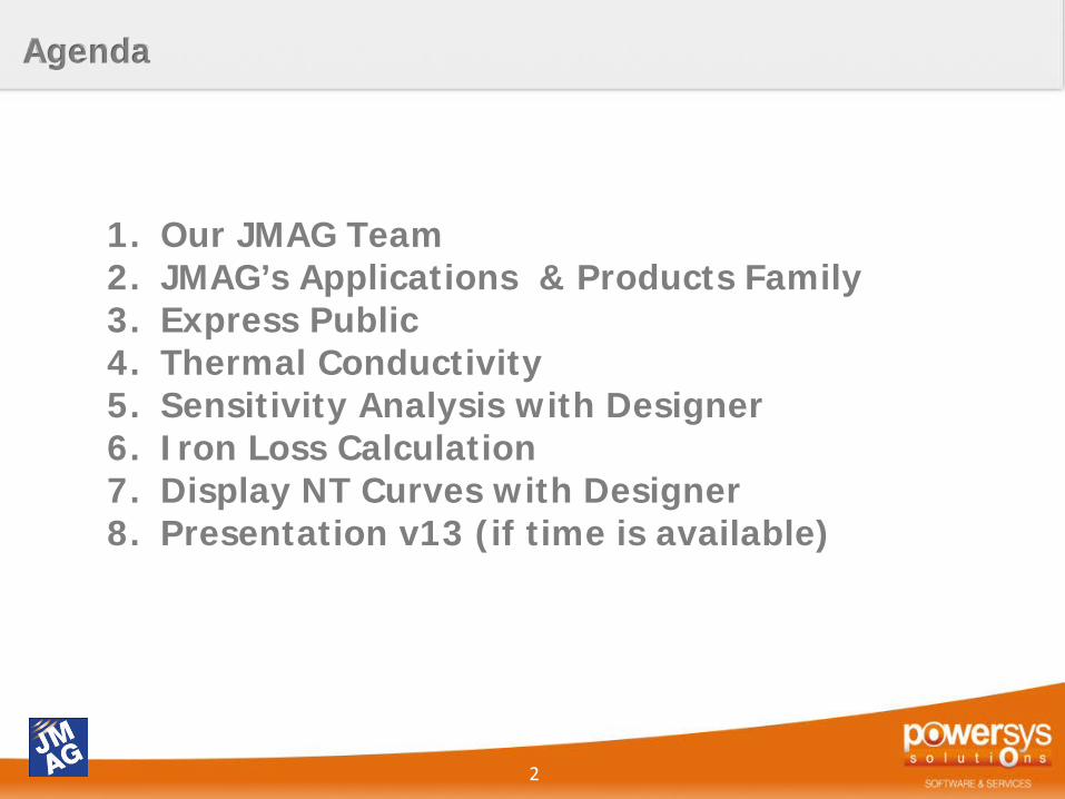
1. Our JMAG Team 2. JMAG’s Applications & Products Family 3. Express Public 4. Thermal Conductivity 5. Sensitivity Analysis with Designer 6. Iron Loss Calculation 7. Display NT Curves with Designer 8. Presentation v13 (if time is available)

Agenda

2

Our JMAG Team

1

JMAG is developed by JSOL Corporation with headquarters in

Tokyo, Japan:

30 years of software development

4

• JSOL Corporation: 1300 employees

• JSOL’s dedicated JMAG employees: 65

• 600 user sites for JMAG worldwide

• Global partner network

JMAG Distribution

5

JSOL works with a global distribution network

Geometry Modeling Generating Mesh Material Modelling Magnetic Field Analysis Multiphysics (Structural, Themal analysis) Running Analysis Post-Processing

Inuitive GUI Model Feedback (CAD Diagnostic System, Conditions Checks, Analysis Monitor) Automation Parametric Calculation Optimization Analysis Reports Scripting Universal Batch System

Highly efficient iterative Solver for both 2D and 3D models Parallel Solver Distributed Analysis Remote Execution

Major CAD Links File Import/Export Script Links to Third-Party products Real Time Simulators System Level Simulators Drive/Control simulators Optimizers

PRECISE ANALYSIS HIGH SPEED PROCESSING

HIGH PRODUCTIVITY OPEN INTERFACE

JMAG Capabilities – Our Moto

6

Automotive

7

Selection of JMAG users

Power Electronics and other industries

JMAG Product family

2

JMAG ElectroMagnetic Platform

Manual Set Up Automated Set Up

Basic Model

Complex Model

Common motor templates Easy to set up Generates basic characteristics

Customizable motor templates Easy to set up Generates basic characteristics Predefined analysis scenarios Automatically produce standard metrics

Can use any geometry Most powerful analysis tool Automation via scripting

Use predefined analysis scenarios Input JMAG Designer model Automate the analysis/design process

JMAG Designer

JMAG Express JMAG Express PM

JMAG Virtual Test Bench

Work together and with 3rd party software

RT & RT-Viewer +

Set Geometry, Conditions, material and Drive OR

use the Sizing Function

Click Solve to Automatically Display Results

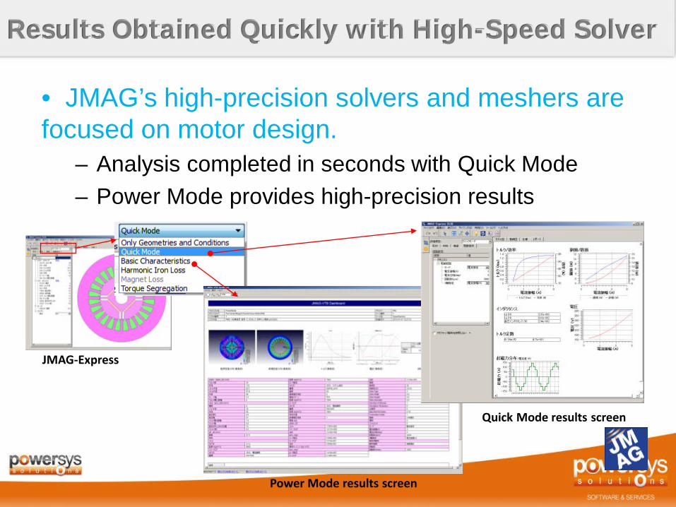
Results Obtained Quickly with High-Speed Solver

• JMAG’s high-precision solvers and meshers are focused on motor design.

– Analysis completed in seconds with Quick Mode – Power Mode provides high-precision results

JMAG-Express

Power Mode results screen

Quick Mode results screen

Current phase-torque properties

Torque-speed curve

Efficiency map

Voltage waveform Cogging torque

Magnetic flux eddy current loss

Magnetic flux distribution

Results are displayed automatically!

14

A JMAG-RT model is… – A high fidelity motor model for SILS/HILS generated from

JMAG FEA. – Available before having real machines so that Model

Based Design (MBD) is realized.

Bypass

FEA model Machine design

Control design

An RT file contains a device’s performance data

JMAG RT Viewer allows users to quickly create visual representations of the RT model data.

Visual representation Data

Can display D and Q axis inductance

versus current versus phase angle

by choosing a basic control method torque vs speed efficiency vs speed

RT Viewer uses simplified control algorithms to simulate a machine’s performance

Most users run the same analyses on every new model. VTB automate the analyses !!

17

Automating the analysis process for complex calculation

Step 1: Choose the scenario

Step 2: Import your model to the scenario

Step 3: Run the scenario and evaluate the results

How to use the VTB ?

18

JMAG Designer

The core product of the platform

19

JMAG Capabilities: Analysis Functions & Coupled Analyses

Beyond EM

20

Electric field analysis

Magnetic field analysis

Joule loss analysis

Sound pressure analysis

Vibration analysis

Stress analysis Heat analysis Iron loss analysis

Induction Heating

Express Public : Sensitivity Analysis and optimisation

3

Express Public: Sensitivity Analsis / Optimization

22

1. Open Express Public 2. Select the type of motor

IPM > PM_I_D_I


23

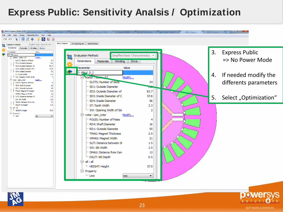
3. Express Public => No Power Mode 4. If needed modify the

differents parameters

5. Select „Optimization“


24

6. Set the first objectiv function Torque > Maximize Revolution speed : 3000 rpm

7. Set (or not) the second objectiv function Iron Loss > Minimize Revolution speed: 3000 rpm


25

8. Set the weighting of each function Stay in the middle

9. Click on Run

10. Get the result of the Sensitivity Analysis


26

11. Select the parameter to Add (several parameter are allow to be selected using the Ctrl Key + Clicking) SD4: Inside Diameter

12. Set the range of the values Minimum: 55 , Maximum: 57 Caution, the value of the parameter(s) need(s) to be coherent with the other parameters If not, the optimisation won‘t be possible and the geometry will be „destroyed“

13. Click on run

14. Get the Optimized value(s) which correspond to the Objective Function (s)

Thermal Conductivity

4

Thermal Conductivity of a basic geometry

1. Open JMAG Designer 2. Open the Geometry Editor and Create the geometry


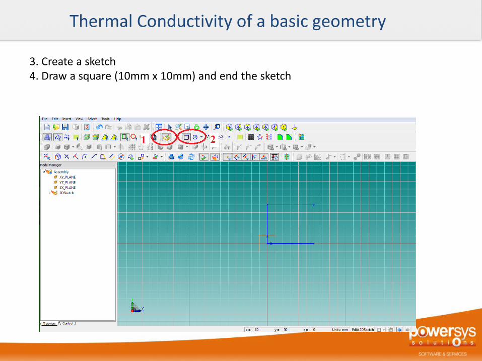
3. Create a sketch 4. Draw a square (10mm x 10mm) and end the sketch


5. Create a new sketch 6. Create a second square ( 1mm gap between the two)


6. End the sketch Edit Mode 7. Move each sketch to a new part


For each part: 8. Get in Edit Mode 9. Select the „Extrude Tool“ and extrude from 10mm 10. Go back to Designer and Import the model


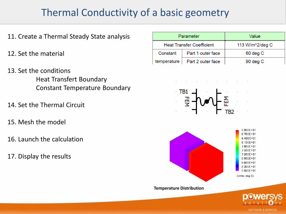
11. Create a Thermal Steady State analysis 12. Set the material 13. Set the conditions Heat Transfert Boundary Constant Temperature Boundary 14. Set the Thermal Circuit 15. Mesh the model 16. Launch the calculation 17. Display the results

Temperature Distribution

Sensivity Analysis with JMAG Designer

5

1. Open Designer and load the following model: SensitivityAnalysis.jproj

2. Click on Run all Cases

Sensitivity Analysis of Dimensional Tolerance in an SPM Motor


Cogging Torque

Frequency Component of Cogging Torque


Induced Voltage

Frequency Component of thee induced Voltage

Iron Loss Calculation

6

Open JMAG Designer and load the following model: IronLossAnalysis.jproj

The regular magnetic results are included in the model.


2) The magnetic flux density behavior in the rotor and in the stator is different. Two measuring points could be reviewed.

So two different iron loss calculations will be performed.


3) Right-click on the study and select “New Loss study”:

New loss

study.


4) Allow iron loss calculation only on the stator:


5) In the properties of the iron loss study, specify the following settings:


6) The calculation can be run and the results displayed:


7) The same procedure should be performed for the rotor with the following settings:


52

8) The calculation can be run and the results displayed:


53

9) From the tables, some values could final be extracted:


Display an NT Curves with Designer

7

1) Open the Model : 2DModel_NT_Curves.jproj 2) Check out the model parameters, conditions,materials..


Partial model: ¼ 4 poles 24 slots Please note that the there is a FEM conductor on the magnet in order to take into account of the Eddy current

3) Check out the circuit (Load calculation)


Please note that the there is a FEM conductor in the circuit which is link to the FEM conductor from the magnet

4) Mesh the model: Rotation Periodic Mesh is applied => accurate mesh in the AG so well adapted for Torque Calculations


5) Create the parametric analysis a) Case Control > Select Parameter

i. In the Study Properties, select: Step / Time step ii. In the conditions, select: Constant revolution speed

b) Case Control > Equation i. Create the variable S as a [Value] link with the rotation condition ii. Create the variable T as an expression link with the time step


5) Create the parametric analysis a) Case Control > Create cases

i. For S, change the Type to increment ii. Edit an increment of 1000 and 3 steps iii. Generate the cases


5) Run all cases


5) In the results, display the Graph of the Torque 6) Select Response Graph Data as a Simple Average


7) Torque Data are display in the Response Graph Data in the the results 8) Right click on Response Graph Data > Graph and then Generate 9) Give the parameters from the axis.


10) Display the graph


V13

8

Thank for your

attention!!

Any questions?

Contacts

www.powersys-solutions.com www.jmag-international.com

magnetik 4 freaks - hochschule heilbronn · pdf filemagnetik 4 freaks 27th of november, 2013...

Documents