macroeconomic shocks and policies - world...
TRANSCRIPT

Macroeconomic Shocks and Policies
B. Essama-Nssah
355
7
The importance of distributional issues in policymaking creates a needfor empirical tools that can help assess the impact of economic shocksand policies on the living standards of relevant individuals. The purpose
of this chapter is therefore to review some of the modeling approaches thatare currently in use at the World Bank and other international financialinstitutions in the evaluation of the impact of macroeconomic shocksand policies on poverty and income distribution. The hope is that theinterested reader might then be able to make an informed choice amongthe reviewed approaches.1
Developing countries face a host of macroeconomic challenges in thedesign and implementation of development strategies and policies. Someof the recurrent issues include (1) fiscal adjustment, (2) monetary policyreforms, (3) trade liberalization, and (4) the impact of terms-of-tradeshocks. Fiscal adjustment involves a modification of government tax,spending, and borrowing policies to achieve a sustainable macroeconomicframework consistent with the objectives of economic growth and povertyreduction. Monetary policy reforms entail control of foreign capital flowsand adjustments in the money supply and in the exchange rate. Tradeliberalization implies a reduction or removal of trade barriers such asquantitative restrictions and tariffs. In fact, trade liberalization has
The author is grateful to Stefano Paternostro, Aline Coudouel, Vijdan Korman, MoatazMostafa Kamel El Said, Hans Löfgren, Delfin S. Go, Oleksiy Ivaschenko, David P. Coady,Limin Wang, and Philippe H. Le Houerou for useful suggestions and insightful commentson an earlier draft. Vijdan Korman also provided excellent support during the preparationof this chapter.
become a prerequisite for participation in the World Trade Organization.Finally, terms-of-trade shocks are important determinants of the perfor-mance of open economies. Many developing countries are, indeed, pri-mary commodity exporters or net oil importers and hence vulnerable tovolatility in the world prices of these commodities.
The need to consider the distributional implications of such macro-economic events stems from at least two basic considerations related tothe goal of development and the heterogeneity of the stakeholders. In thecontext of the Millennium Declaration (United Nations 2000), the inter-national community has included poverty and hunger eradication amongthe basic objectives of development and has thus made poverty reductiona benchmark measure of the performance of socioeconomic systems.This vision is consistent with the notion of development as empower-ment, meaning a process that entails the expansion of the ability of par-ticipants to achieve their freely chosen life plans. In this perspective,poverty is seen as the deprivation of basic capabilities to live the kind oflife that one has reason to value (Sen 1999).
Furthermore, political factors are essential determinants of eco-nomic outcomes, and distributional issues underpin the political dimen-sion of policymaking (understood to include implementation) becauseof the heterogeneity of interests. Heterogeneity may stem from differ-ences in tastes, in resource endowments, or in views of the world. Therecould be conflicts of interest even in situations where the socioeconomicagents are identical ex ante. They may value a good equally, yet be in con-flict over the distribution of the good (Drazen 2000). Approaches to pol-icymaking may be characterized according to whether they account forpolitical constraints arising from a heterogeneity of interests. With noconflict of interest, optimal policies could be found by maximizing theutility of a representative agent. This is essentially the normative approachto policymaking (Dixit 1996). In the positive approach, policymaking isconsidered a political process involving strategic interactions among var-ious socioeconomic agents subject to potential conflict over distribution.
Two basic dimensions define the desirable properties of a policy model:relevance and reliability (Quade 1982). A relevant model focuses on issues ofconcern and on politically significant socioeconomic groups and the inter-actions among them. A reliable model is based on sound analytical linkagesbetween available policy instruments (part of the exogenous variables) andrelevant outcomes such as poverty or inequality (part of the endogenousvariables) to ensure a high degree of confidence in the model’s predictions.Modeling the poverty and distributional impacts of macroeconomicshocks and policies therefore requires a clear understanding of the transmis-
Analyzing the Distributional Impact of Reforms
356
sion channels. This relates to the specification of the linkages among macro-economic shocks and policies, as well as the fundamental determinants ofthe distribution of economic welfare. In the terminology of Bourguignon,Ferreira, and Lustig (2005), macroeconomic events may have three types ofeffects on income distribution: (1) endowment effects represent changes inthe amounts of the resources available to individuals or households; (2) priceeffects translate changes in the remuneration of these resources; (3) finally,occupational effects represent changes in resource allocation.
The outline of the chapter is as follows. The following section focuseson simulation models of the size distribution of an indicator of economicwelfare. In the section, two types of approaches to modeling the size dis-tribution of economic welfare across a population are reviewed. The firstincludes purely statistical models such as POVCAL (Chen, Datt, andRavallion 1991) and SimSIP Poverty (Wodon, Ramadas, and Van derMensbrugghe 2003). These two tools rely on a parameterization of theLorenz curve and, arguably, offer the simplest way of simulating the povertyeffect of macroeconomic shocks and policies. The second approach relieson unit record data and includes (1) PovStat (Datt and Walker 2002), (2) themaximum value or envelope model2 (Chen and Ravallion 2004; Ravallionand Lokshin 2004), and (3) the household income and occupational choicemodel (Bourguignon and Ferreira 2005).
The subsequent section discusses poverty and distributional analysiswithin a general equilibrium framework (Dervis, de Melo, and Robinson1982; Decaluwé et al. 1999).
The penultimate section examines modular approaches to linkingmacroeconomic models to models of income distribution. The sectionfocuses on the 123PRSP model—the name stands for one country, twosectors, and three commodities, and the model is built to feed into themacroeconomic framework for Poverty Reduction Strategy Papers—(Devarajan and Go 2003); the Poverty Analysis Macroeconomic Simu-lator I (PAMS I) (Pereira da Silva, Essama-Nssah, and Samaké 2003);PAMS II (Essama-Nssah 2004, 2005); a macro-micro simulation modelfor Brazil that uses the investment savings–liquidity money (IS-LM)framework for macroeconomic analysis (Ferreira et al. 2004); and theintegrated macroeconomic model for poverty analysis (IMMPA) frame-work, which links a dynamic computable general equilibrium (CGE)model to unit record data (Agénor, Izquierdo, and Jensen 2006).
Concluding remarks are presented in the last section. Table A7.1 in theannex provides a summary description of the tools reviewed in this chapter.
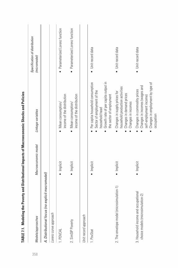
Table 7.1 presents a synoptic view of the modeling approachesdescribed in this chapter, with a focus on three elements: the treatment
Macroeconomic Shocks and Policies
357
358
TAB
LE7.
1.M
odel
ing
the
Pove
rty
and
Dis
trib
utio
nalI
mpa
cts
ofM
acro
econ
omic
Shoc
ksan
dPo
licie
s
Spec
ifica
tion
ofdi
strib
utio
nM
odel
s/ap
proa
ches
Mac
roec
onom
icm
odel
Link
age
varia
bles
(mic
rom
odel
)
A.Di
strib
utio
nalf
ocus
(no
expl
icit
mac
rom
odel
)
Lore
nzcu
rve
appr
oach
1.PO
VCAL
2.Si
mSI
PPo
verty
Unit
reco
rdap
proa
ch
1.Po
vSta
t
2.Th
een
velo
pem
odel
(mic
rosi
mul
atio
n-1)
3.Ho
useh
old
inco
me
and
occu
patio
nal
choi
cem
odel
s(m
icro
sim
ulat
ion-
2)
•Im
plic
it
•Im
plic
it
•Im
plic
it
•Im
plic
it
•Im
plic
it
•M
ean
cons
umpt
ion/
inco
me
ofth
edi
strib
utio
n
•M
ean
cons
umpt
ion/
inco
me
ofth
edi
strib
utio
n
•Pe
rcap
itaho
useh
old
cons
umpt
ion
•Se
ctor
ofem
ploy
men
toft
heho
useh
old
head
•Gr
owth
rate
ofpe
rcap
itaou
tput
inth
ese
ctor
ofem
ploy
men
t
•Ch
ange
sin
supp
lypr
ices
for
hous
ehol
dpr
oduc
tion
activ
ities
•Ch
ange
sin
dem
and
pric
es•
Chan
gesi
nin
com
es
•Ch
ange
sin
com
mod
itypr
ices
•Ch
ange
sin
inco
mes
(wag
esan
dse
lf-em
ploy
men
tinc
ome)
•Ch
ange
sin
empl
oym
entb
ytyp
eof
occu
patio
n
•Pa
ram
eter
ized
Lore
nzfu
nctio
n
•Pa
ram
eter
ized
Lore
nzfu
nctio
n
•Un
itre
cord
data
•Un
itre
cord
data
•Un
itre
cord
data

359
B.St
anda
rdge
nera
lequ
ilibr
ium
anal
ysis
1.CG
E–re
pres
enta
tive
hous
ehol
d
2.CG
E–ex
tend
edre
pres
enta
tive
hous
ehol
d
C.Se
quen
tialm
acro
-mic
rolin
kage
s
1.PA
MS
I
2.PA
MS
II
3.12
3PRS
P
4.CG
E-m
icro
sim
ulat
ion-
1
•St
atic
CGE
•St
atic
CGE
•Re
vise
dm
inim
umst
anda
rdm
odel
exte
nded
(RM
SM-X
)
•St
atic
CGE
mod
el
•Fi
nanc
ialp
rogr
amm
ing
mod
el•
Grow
thm
odel
s•
123C
GEm
odel
•St
atic
CGE
mod
el
•Ch
ange
sin
fact
oran
dco
mm
odity
pric
es•
Chan
gesi
nem
ploy
men
t
•Ch
ange
sin
fact
oran
dco
mm
odity
pric
es•
Chan
gesi
nem
ploy
men
t
•Gr
owth
rate
ofou
tput
•Ch
ange
sin
sect
oral
wag
es•
Chan
gesi
ndi
spos
able
inco
me
bygr
oup
•Ch
ange
sin
fact
oran
dco
mm
odity
pric
es•
Chan
gesi
nem
ploy
men
t•
Hous
ehol
d-le
velr
ealc
onsu
mpt
ion
•Ch
ange
sin
com
mod
itypr
ices
•Ch
ange
sin
inco
mes
•Ch
ange
sin
fact
oran
dco
mm
odity
pric
es•
Chan
gesi
nin
com
es
•A
few
repr
esen
tativ
eho
use-
hold
s
•A
few
repr
esen
tativ
eho
use-
hold
s•
Am
odel
ofsi
zedi
strib
utio
n
•Un
itre
cord
data
•Un
itre
cord
data
•Pa
ram
eter
ized
Lore
nzfu
nctio
n
•Un
itre
cord
data
•En
velo
pem
odel
•Un
itre
cord
data
•En
velo
pem
odel
( con
tinue
d)

360
5.CG
E-m
icro
sim
ulat
ion-
2
6.IS
-LM
mic
rosi
mul
atio
n-2
7.IM
MPA
Sour
ce:
Com
pile
dby
the
auth
or.
TAB
LE7.
1.M
odel
ing
the
Pove
rty
and
Dis
trib
utio
nalI
mpa
cts
ofM
acro
econ
omic
Shoc
ksan
dPo
licie
s(C
ontin
ued
) Spec
ifica
tion
ofdi
strib
utio
nM
odel
s/ap
proa
ches
Mac
roec
onom
icm
odel
Link
age
varia
bles
(mic
rom
odel
)
•St
atic
CGE
mod
el
•IS
-LM
mod
el
•Dy
nam
icCG
Em
odel
with
afin
anci
alse
ctor
•Ch
ange
sin
com
mod
itypr
ices
•Ch
ange
sin
inco
mes
(wag
esan
dse
lf-em
ploy
men
tinc
ome)
•Ch
ange
sin
empl
oym
entb
ytyp
eof
occu
patio
n
•Ch
ange
sin
com
mod
itypr
ices
•Ch
ange
sin
inco
mes
(wag
esan
dse
lf-em
ploy
men
tinc
ome)
•Ch
ange
sin
empl
oym
entb
ytyp
eof
occu
patio
n
•Re
algr
owth
rate
sin
perc
apita
cons
umpt
ion
and
disp
osab
lein
com
efo
rsix
repr
esen
tativ
eho
useh
olds
•Un
itre
cord
data
•Ho
useh
old
inco
me
and
occu
pa-
tiona
lcho
ice
mod
els
•Un
itre
cord
data
•Ho
useh
old
inco
me
and
occu
pa-
tiona
lcho
ice
mod
els
•Un
itre
cord
data

of the macroeconomic framework, the modeling of the size distribution,and the variables linking the macroeconomic framework to the model ofdistribution. The first category has no explicit macromodel. The secondembeds distributional mechanisms in a general equilibrium model.
The last approach links a macroeconomic model to a distributionmodel in a top-down fashion. All the models reviewed fall within the classof policy models. The specification of such models is dictated by theissues at stake, the knowledge about the nature of the process involved,and the availability and reliability of relevant data. It is impossible to pro-vide, in the context of an overview like this one, enough implementationdetails for each model under consideration. However, an effort has beenmade to include a long list of relevant references, as well as boxes describ-ing examples of the approaches. In addition, the annex to this chaptersupplies a description of many of the tools considered. It also includes anestimation of the cost of implementation and information on appropriatesoftware for some of the tools.
SIMULATION MODELS OF THE SIZE DISTRIBUTION OF INCOME
The idea of simulating the distribution of income among individuals orhouseholds originated in the field of public finance because of the needto have reliable models for the detailed analysis of the incidence of atax-benefit system. The basic idea is to model the distribution of house-hold income and consumption taking household behavior as exogenous,but fully accounting for applicable taxes and transfers (Davies 2004). Toreflect the diversity of the characteristics in a population adequately, thesesimulation models require a nationally representative microdata set. Thefact that household behavior is exogenous means that these accountingmodels can predict only the first-round effects of a tax-benefit policy oninequality and poverty.
All the approaches reviewed in this section are various interpreta-tions of the basic idea underlying tax-benefit simulation models. POV-CAL and SimSIP Poverty illustrate the use of the Lorenz curve for povertyand distributional impact analysis. These two tools are particularly use-ful when only aggregate or grouped data are available. The second classof simulation tools considered under this heading relies on unit recorddata on the distribution of some money-metric measure of economicwelfare at the individual or household level. Three approaches are exam-ined. PovStat uses per capita consumption as a measure of welfare. Thesecond approach relies on the envelope theorem and employs the maximumvalue function to model the determinants of individual welfare (Chen and
Macroeconomic Shocks and Policies
361
Ravallion 2004; Ravallion and Lokshin 2004). The last approach is basedon a reduced-form model of household income generation (Bourguignonand Ferreira 2005). Even though the envelope model and the income-generation models include some aspects of household behavior, thesemicrosimulation models must be viewed as statistical devices to the extentthat they fail to account fully for market adjustment through endogenousprices or the adjustment of the behavior of agents from one equilibriumstate to another (Ferreira and Leite 2003).
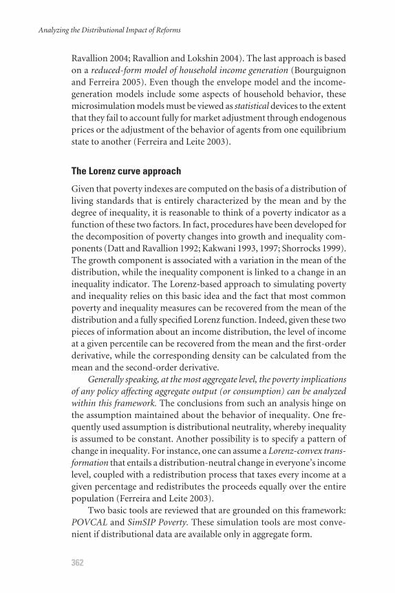
The Lorenz curve approach
Given that poverty indexes are computed on the basis of a distribution ofliving standards that is entirely characterized by the mean and by thedegree of inequality, it is reasonable to think of a poverty indicator as afunction of these two factors. In fact, procedures have been developed forthe decomposition of poverty changes into growth and inequality com-ponents (Datt and Ravallion 1992; Kakwani 1993, 1997; Shorrocks 1999).The growth component is associated with a variation in the mean of thedistribution, while the inequality component is linked to a change in aninequality indicator. The Lorenz-based approach to simulating povertyand inequality relies on this basic idea and the fact that most commonpoverty and inequality measures can be recovered from the mean of thedistribution and a fully specified Lorenz function. Indeed, given these twopieces of information about an income distribution, the level of incomeat a given percentile can be recovered from the mean and the first-orderderivative, while the corresponding density can be calculated from themean and the second-order derivative.
Generally speaking, at the most aggregate level, the poverty implicationsof any policy affecting aggregate output (or consumption) can be analyzedwithin this framework. The conclusions from such an analysis hinge onthe assumption maintained about the behavior of inequality. One fre-quently used assumption is distributional neutrality, whereby inequalityis assumed to be constant. Another possibility is to specify a pattern ofchange in inequality. For instance, one can assume a Lorenz-convex trans-formation that entails a distribution-neutral change in everyone’s incomelevel, coupled with a redistribution process that taxes every income at agiven percentage and redistributes the proceeds equally over the entirepopulation (Ferreira and Leite 2003).
Two basic tools are reviewed that are grounded on this framework:POVCAL and SimSIP Poverty. These simulation tools are most conve-nient if distributional data are available only in aggregate form.
Analyzing the Distributional Impact of Reforms
362

POVCAL
The following types of simulations can be performed using POVCAL(Datt 1992, 1998): (1) sensitivity analysis with respect to the poverty line,(2) analysis of the poverty implications of distributionally neutral growth,(3) decomposition of poverty changes into growth and redistributioncomponents, plus a residual, and (4) the contribution to overall povertyof regional or sectoral disparities in mean consumption. As far as policyanalysis is concerned, POVCAL can be used to trace the poverty and dis-tributional implications of any policy that affects the overall mean or thesectoral means.
This tool presents two major limitations for the analysis of the dis-tributional impact of macroeconomic shocks and policies: the modelingof the macroeconomic framework remains implicit, and the level ofaggregation of the household level limits the ability of the tool to accountfor heterogeneity.
For POVCAL, data are expected to be structured in “records” and“subgroups.”3 The number of records is determined by the number ofclass intervals or quantiles in the data. A data set presented in deciles con-tains 10 records. The number of subgroups corresponds to the number ofexhaustive and mutually exclusive socioeconomic groups, for example,rural and urban households.4
Eight data configurations are possible: (1) the cumulative proportionof individuals and the corresponding cumulative proportion of income;(2) the proportion of the population and the associated proportion ofincome; (3) the cumulative proportion of the population and the pro-portion of income; (4) the proportion of the population and the cumu-lative proportion of income; (5) the percentage of people in a given classinterval and the class mean income; (6) the upper bound of the class inter-val, the percentage of the population in the class, and the class meanincome; (7) the upper bound of the class interval, the cumulative propor-tion of the population in the class, and the class mean income; and (8) theupper bound of the class interval and the percentage of the populationin the class.
When the class mean income is unknown, the following rule of thumbis recommended (Chen, Datt, and Ravallion 1991): (1) set the mean forthe poorest class at 80 percent of the upper bound of that class interval;(2) set the mean of the highest class at 30 percent above the lower boundof that class; and (3) use the midpoint for all other classes.
POVCAL will prompt the user for five key inputs: (1) the name ofthe ASCII input data file, (2) the number of subgroups, (3) the numberof records, (4) the type of data configuration (codes 1 through 8), and
Macroeconomic Shocks and Policies
363
(5) the DOS name for the output file. Once this input has been receivedfor each of the two specifications of the Lorenz curve underlying the simu-lation tool, the program provides an estimate of the Lorenz curve, alongwith relevant statistical summary measures. It prompts the user to sup-ply a poverty line and a different estimate of the mean of the distribution(if he/she does not want to use the estimate based on the data).
An application of POVCAL is illustrated in Box 7.1.It is important to make sure that the poverty line is expressed in the
same units as the mean of the distribution. The program then computesthe Gini index of inequality, poverty measures of the Foster-Greer-Thorbecke (1984) family, and the associated elasticities with respect to themean and the Gini index. The computation of the elasticities with respectto the Gini index assumes a Lorenz-convex transformation whereby theLorenz curve shifts proportionately up or down at all points. Finally, theprogram plots the fitted Lorenz curves and the corresponding first andsecond derivatives and provides an assessment of the Lorenz curve thatseems to fit the data most closely.
SimSIP Poverty
SimSIP Poverty is a member of the SimSIP family of simulation tools, acollection of Excel-based modules designed to simulate social indicatorsand poverty. The following inputs are expected for the tool: (1) incomeor consumption distribution by groups (deciles or quintiles), (2) the meanincome or consumption for each group, (3) the population shares for eachgroup, and (4) the relevant poverty lines. Depending on data availability,the analysis can be performed at the national level and for socioeconomicgroups classified by place of residence (urban or rural) or by sector ofemployment (agriculture, manufacturing, and services).
The key limitation on SimSIP Poverty arises because changes in per capita income (or expenditure) and the linkages between macro-economic shocks and policies are exogenous. The tool thus imposes aminimal structure upon the complex relationship between policy instru-ments and poverty outcomes. No behavioral or market adjustment ismodeled explicitly. The reliability of the predictions of the simulator thusdepends on the modeling of the process that engendered the changes inthe means and the accuracy of the population shares that are fed into thesimulator. Another limitation is due to the requirement that the inputdata be aggregated. This implies a loss of information with respect to theheterogeneity of households. In fact, SimSIP Poverty shares these limita-tions with POVCAL.
The use of SimSIP Poverty is illustrated in Box 7.2.
Analyzing the Distributional Impact of Reforms
364

Macroeconomic Shocks and Policies
365
BOX 7.1 Lorenz Curve Approach, POVCAL: Assessing Poverty Dynamics in Madagascar
Essama-Nssah (1997) uses POVCAL to analyze the dynamics of poverty in Madagascarbetween 1962 and 1980. Over this period, different governments showed various levels ofconcern over poverty issues. Some of the policy choices targeted either the rural or theurban sector. From the early 1960s to the mid-1970s, public policy favored the rural sectorby lifting the poll and cattle tax applicable to the sector and by providing farmers freeaccess to agricultural inputs. In 1977, an urban bias was introduced in public policy whenthe government increased the minimum wage and decided to subsidize basic items such asrice, edible oils, and condensed milk.
The study is based on two published aggregated data sets on income distribution in the ruraland urban sectors. These data are in the form of class intervals with the associated frequencyand mean incomes. The analysis through POVCAL revealed that, while poverty in Madagascarremained a predominantly rural phenomenon, poverty generally increased between 1962 and1980 in both rural and urban areas. A decomposition of the poverty outcomes into growth andinequality components showed that increased income inequality in the rural sector was themajor cause of the observed increase in rural poverty (see Table 7.2). In the urban sector,however, increased poverty was most likely due to the lack of economic growth.
The study concluded that the urban bias introduced into government social policies in themid-1970s was not justifiable strictly on grounds of poverty reduction. A simulation of whatthe level of poverty would have been had rural and urban mean incomes been set to thenational average showed that a significant reduction in aggregate poverty could have beenachieved had the government pursued effective policies to lessen the regional disparities.
TABLE 7.2. Poverty Measures and the Decomposition of Poverty Outcomes, Madagascar, 1962–80
Value Value Measure (1962) (1980) Change Growth Inequality Residual
RuralHeadcount 46.65 42.25 −4.40 −17.72 6.24 7.08Poverty gap 10.50 15.24 4.74 −5.67 10.29 0.12Squared 3.15 7.51 4.36 −2.06 7.68 −1.26
poverty gap
UrbanHeadcount 13.35 18.47 5.12 9.74 −1.34 −3.28Poverty gap 2.72 6.73 4.01 3.88 1.20 1.07Squared 0.73 3.31 2.58 1.73 1.00 −0.15
poverty gap
Source: Essama-Nssah 1997.

BOX 7.2 Lorenz Curve Approach, SimSIP Poverty: Predicting the Effect of Aggregate Growthon Poverty in Paraguay
366
Datt et al. (2003) have applied SimSIP Poverty to data for Paraguay in order to study theimpact of growth patterns on poverty for a period of five years (from 1997 to 2001). Six cases are considered: (1) each sector (agriculture, industry, services) of the economygrows at 3 percent, (2) a 2 percent growth rate in each sector, (3) a 1 percent growth rateper sector, (4) a 2 per percent growth rate in agriculture and a 3 percent rate elsewhere,(5) a 1 percent growth in agriculture and a 3 percent rate elsewhere, and, finally, (6) a 3 percentgrowth in agriculture and a 1 percent rate in other sectors. The underlying data include(1) population shares by sectors (rural/urban) and three economic activities (agriculture,industry, and services), as well as the total national-level population, and (2) the meanincome per capita corresponding to the population shares.
The impact of different sectoral growth patterns on the poverty headcount is reported inTable 7.3. Holding inequality constant, a 3 percent annual growth in per capita income inevery sector for five years would reduce poverty by 3 percentage points, to 28.95 percent.Using the table, one can compare the contribution of different growth patterns to povertyreduction. Moreover, given that poverty rates are higher in rural areas and in agriculture, anymigration out of those sectors is likely to decrease poverty.
The reported results for each scenario vary slightly depending on whether aggregate povertyis computed from the rural/urban perspective or as a weighted average of outcomes in eachsector of employment. The exercise illustrates the fact that the analyst may use SimSIPPoverty to assess different patterns of growth.
TABLE 7.3. Simulations of the Impact of Growth Patterns on Poverty in Paraguay: Some Examples
Period 2: Period 2: national as national as
National Period 2: weighted average weighted average poverty national of urban/rural of employment headcount, % Period 1 simulation sectors sectors
3% per sector for five years 32.13 27.46 27.48 27.42
2% per sector for five years 32.13 28.95 28.97 28.92
1% per sector for five years 32.13 50.51 30.53 30.49
2% in agriculture, rural sector, 3% elsewhere for five years 32.13 – 28.15 27.94
1% in agriculture, rural sector, 3% elsewhere for five years 32.13 – 28.82 28.46
3% in agriculture, rural sector, 1% elsewhere for five years 32.13 – 29.06 29.34
Source: Datt et al. 2003.
Computations are based on a parameterization of the Lorenzcurve. Two parameterizations are provided by the general quadraticand the Beta models. For robust poverty comparisons over time andamong sectors, the simulator produces poverty dominance and Lorenzcurves. It also computes the Gini coefficient, poverty measures of theFoster-Greer-Thorbecke family, and the associated elasticities withrespect to growth and inequality. Any member of this family for a givengroup can be written as a weighted sum of poverty within all the sub-groups. The weights are equal to the population shares. Based on thisfact, SimSIP Poverty provides decompositions of poverty outcomes inthree components. The first component represents change in within-group poverty. The second term measures the effects of populationshifts among groups. The last component captures the interactionbetween inter- and within-group effects (see Ravallion and Huppi 1991for details). It is also possible to decompose changes in poverty overtime into the following contributing factors: growth, inequality, and aresidual. These decompositions require two sets of observations on thedistribution of income or expenditure. This is the same approach dis-cussed above in the case of POVCAL.
Unit-record-based approaches
PovStat
PovStat is an Excel-based tool primarily designed to simulate thepoverty implications of alternative growth paths. This simulation toolarose out of the basic idea that the rate and pattern of economicgrowth determine the evolution of poverty over time. In particular, itis assumed that per capita consumption for a household grows at the samerate as per capita output in the sector of employment of the head of thehousehold. Households are classified into four sectors on the basis ofthe employment status of the head: (1) agriculture, (2) industry, (3)services, and (4) residual. The residual sector amalgamates householdswith unemployed or inactive heads and those with unknown occupa-tional status.
A major advantage of PovStat over SimSIP Poverty stems from theuse of unit-level data. This has the potential to improve the precisionof the estimates of the poverty and inequality measures. Otherwise, thetool shares in the major limitations that have been flagged for POV-CAL and SimSIP Poverty: (1) there is no explicit modeling of themacroeconomic framework, and (2) there is a loss of informationabout the heterogeneity of households because the sectoral classifica-tion of households is based on the status of the heads of household.
Macroeconomic Shocks and Policies
367

Finally, the flexibility provided in setting assumptions about changesin inequality comes at the price of an increased uncertainty in theresults.
The two key inputs are country-specific unit record household-leveldata representing the distribution of living standards for a base year anda set of user-supplied projection parameters characterizing the paths ofgrowth. Household-level data involve six variables that must be submit-ted to the simulator in the following order: (1) a household identifier, (2)monthly per capita consumption in local currency units for the base year,(3) household weight (or a population expansion factor), (4) an urbandummy, (5) household size, and (6) sector of employment of the house-hold head.
For each year within the projection horizon, the per capita consump-tion for each household is computed recursively using a growth rate that isequal to the rate of per capita output. The latter is calculated as the realgrowth in gross domestic product (GDP) in the sector of employment of thehead of household, minus the rate of population growth in that sector. Forthe first three sectors, the sectoral population growth rate is computed fromthe overall population growth rate and an adjustment factor that dependson the share of each sector in total employment and sector-specific growthrates of employment. The population in the residual sector is assumed togrow at the same rate as the overall population. Household weights are alsoadjusted recursively using sectoral rates of population growth.
Assuming that inequality within sectors remains constant, PovStatcomputes the following indicators for the forecast horizon: (1) povertymeasures of the Foster-Greer-Thorbecke family, (2) the number of peo-ple below the poverty line, (3) mean monthly per capita consumption,(4) Gini coefficients, (5) two inequality measures of the generalizedentropy family, and (6) the variance of log consumption per person.
In general, the simulation framework offers the user the opportunityto control the simulation process by setting the following parameters: (1)the forecast horizon, (2) the poverty line, (3) the base and survey years,(4) the survey-year population, (5) the country’s purchasing power par-ity exchange rate, (6) the base and survey-year consumer price indexes(CPIs), (7) the sectoral output growth rates for each projection year, (8)the population growth rates and employment growth rates for each pro-jection year, (9) the survey-year sectoral GDP and employment shares,(10) the GDP deflator and the CPI for each projection year, (11) changesin the relative price of food by year, (12) the share of food in the bundledefining the poverty line, (13) the share of food in the CPI, (14) thechange in the Gini within each sector for each projection year, (15)
Analyzing the Distributional Impact of Reforms
368

Macroeconomic Shocks and Policies
369
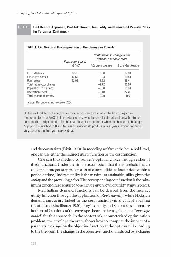
BOX 7.3 Unit Record Approach, PovStat: Growth, Inequality, and Simulated Poverty Pathsfor Tanzania
Tanzania achieved rapid growth in per capita GDP in the 1995–2001 period, but household-budget survey data suggest that the decline in poverty between 1992 and 2001 was rela-tively small. Demombynes and Hoogeveen (2004) argue that a possible explanation for thisoutcome is that poverty increased during the period of economic stagnation in the early1990s, while economic growth in the second half of the 1990s was able to offset only partof the early rise in poverty.
To test this hypothesis, the authors use PovStat to simulate the likely trajectory of povertyrates over the 1992–2002 period. They employ data from two household-budget surveys(1991/92 and 2000/1), along with growth rates derived from national account data. Thesegrowth rates are then applied to unit record data to estimate the full evolution of povertyover the course of the nine-year period.
The simulated poverty trajectories show that poverty rates followed a hump-shaped path duringthe period. Under a variety of scenarios, poverty incidence first increased to above 40 percentin the early 1990s and then declined below 36 percent by 2000/1. The sectoral simulationssuggest that the poverty reduction impact of economic growth in Tanzania was more signifi-cant in urban areas than in rural areas. For example, in Dar es Salaam, economic growthreduced poverty by about 16 percentage points, assuming no change in inequality. In reality,the growth-induced reduction in poverty was partially offset by increased income inequality,which caused poverty to rise by 9.8 percentage points. The sectoral decomposition of thepoverty outcomes also indicates that only a small part (11.6 percent) of the decline in head-count poverty at the national level could be explained by a shift in the population from poorerrural areas to wealthier urban areas such as Dar es Salaam (see Table 7.4). The study con-cludes that achieving the poverty-related Millennium Development Goal by 2015 will requirechanging patterns of growth to include the rural areas where most Tanzanians live.
changes in the average propensity to consume, and (16) the drift betweensurveys and national accounts.
PovStat is illustrated in Box 7.3.
The envelope model
One approach in studying the impact of economic shocks and policies onan economic agent consists in analyzing the impact of those shocks andpolicies on the determinants of the agent’s optimizing behavior. This behav-ior may be characterized in terms of the actions the economic unit can takeand the objective function used to evaluate such actions. The maximumvalue function indicates the maximum attainable value of the objective func-tion in terms of various parameters that enter both the objective function
(continued)
and the constraints (Dixit 1990). In modeling welfare at the household level,one can use either the indirect utility function or the cost function.
One can thus model a consumer’s optimal choice through either ofthese functions. Under the simple assumption that the household has anexogenous budget to spend on a set of commodities at fixed prices within aperiod of time,5 indirect utility is the maximum attainable utility given theoutlay and the prevailing prices. The corresponding cost function is the min-imum expenditure required to achieve a given level of utility at given prices.
Marshallian demand functions can be derived from the indirectutility function through the application of Roy’s identity, while Hicksiandemand curves are linked to the cost function via Shephard’s lemma(Deaton and Muellbauer 1980). Roy’s identity and Shephard’s lemma areboth manifestations of the envelope theorem; hence, the name “envelopemodel” for this approach. In the context of a parameterized optimizationproblem, the envelope theorem shows how to compute the impact of aparametric change on the objective function at the optimum. Accordingto the theorem, the change in the objective function induced by a change
Analyzing the Distributional Impact of Reforms
370
BOX 7.3 Unit Record Approach, PovStat: Growth, Inequality, and Simulated Poverty Pathsfor Tanzania (Continued)
On the methodological side, the authors propose an extension of the basic projectionmethod underlying PovStat. This extension involves the use of estimates of growth rates ofconsumption and population for the quantile and the sector to which the household belongs.Applying this method to the initial year survey would produce a final year distribution that isvery close to the final year survey data.
TABLE 7.4. Sectoral Decomposition of the Change in Poverty
Contribution to change in the
Population share,national headcount rate
1991/92 Absolute change % of Total change
Dar es Salaam 5.50 −0.56 17.08Other urban areas 12.60 −0.34 10.49Rural areas 82.06 −1.82 55.41Total intrasector change −2.72 82.98Population-shift effect −0.38 11.60Interaction effect −0.18 5.41Total change in poverty −3.28 100
Source: Demombynes and Hoogeveen 2004.

in a parameter while the choice variable adjusts optimally is equal to thepartial derivative of the optimal value of the objective function with respectto the parameter (Varian 1984). Thus, the first-order welfare impacts ofchanges in prices can be evaluated on the basis of the indirect utility func-tion by treating quantity choices as given.
According to Roy’s identity, the Marshallian demand function of acommodity is equal to the negative of the first-order derivative of theindirect utility function with respect to the commodity price, divided bythe marginal utility of income. The marginal utility of income is the first-order derivative of the indirect utility function with respect to income.By Shephard’s lemma, the Hicksian demand function is equal to thefirst-order derivative of the cost function with respect to the relevantcommodity price.
These are the key results that allow one to trace the welfare implicationsof any policy that affects commodity prices and household budgets in a waythat also accounts for heterogeneity among households by using household-survey data. Within this simple framework, heterogeneity stems fromdifferences in demand patterns, other sociodemographic characteristicsof households, and the fact that households may face different prices forthe same commodity.
The envelope approach to policy impact analysis has some limitationsbecause one can only capture the static effects of the policy reform. Fur-thermore, the fact that the envelope theorem is valid only in the neighbor-hood of the initial optimum makes the method inappropriate for the studyof large price changes or in situations in which the household is out of equi-librium due to restrictions such as rationing. As noted by Chen and Raval-lion (2004), these cases require an estimation of complete demand andsupply systems. Chen and Ravallion also note that such an estimation ishampered by the general lack of household-level data on prices and wages.
In the context of the envelope approach, a household is assumed tohave preferences among consumption goods and work effort. Thus, thearguments of the utility function include both the quantities of the com-modities consumed and the labor supply by activity (including the house-hold’s own productive activities). The budget to be spent on consumptiongoods is equal to the wage income, plus the profits from household enter-prises. One can see that, on the assumption that a household will opti-mize behavior in both production and consumption, the indirect utilityof the household is a function of the supply prices of the goods the house-hold is selling on the market, the demand prices of the consumption andintermediate goods, and the wage rates in various activities.
An example of the envelope model is provided in Box 7.4.
Macroeconomic Shocks and Policies
371
372
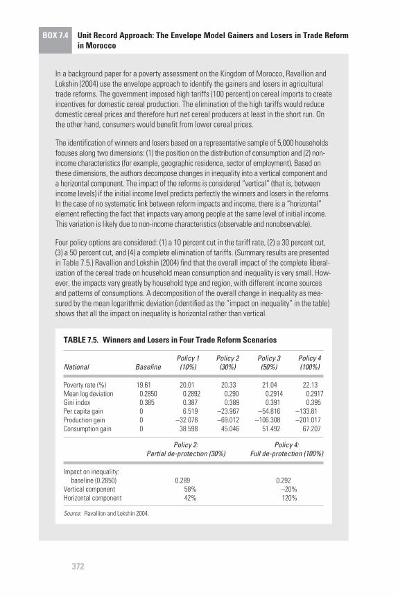
BOX 7.4 Unit Record Approach: The Envelope Model Gainers and Losers in Trade Reformin Morocco
In a background paper for a poverty assessment on the Kingdom of Morocco, Ravallion andLokshin (2004) use the envelope approach to identify the gainers and losers in agriculturaltrade reforms. The government imposed high tariffs (100 percent) on cereal imports to createincentives for domestic cereal production. The elimination of the high tariffs would reducedomestic cereal prices and therefore hurt net cereal producers at least in the short run. Onthe other hand, consumers would benefit from lower cereal prices.
The identification of winners and losers based on a representative sample of 5,000 householdsfocuses along two dimensions: (1) the position on the distribution of consumption and (2) non-income characteristics (for example, geographic residence, sector of employment). Based onthese dimensions, the authors decompose changes in inequality into a vertical component anda horizontal component. The impact of the reforms is considered “vertical” (that is, betweenincome levels) if the initial income level predicts perfectly the winners and losers in the reforms.In the case of no systematic link between reform impacts and income, there is a “horizontal”element reflecting the fact that impacts vary among people at the same level of initial income.This variation is likely due to non-income characteristics (observable and nonobservable).
Four policy options are considered: (1) a 10 percent cut in the tariff rate, (2) a 30 percent cut,(3) a 50 percent cut, and (4) a complete elimination of tariffs. (Summary results are presentedin Table 7.5.) Ravallion and Lokshin (2004) find that the overall impact of the complete liberal-ization of the cereal trade on household mean consumption and inequality is very small. How-ever, the impacts vary greatly by household type and region, with different income sourcesand patterns of consumptions. A decomposition of the overall change in inequality as mea-sured by the mean logarithmic deviation (identified as the “impact on inequality” in the table)shows that all the impact on inequality is horizontal rather than vertical.
TABLE 7.5. Winners and Losers in Four Trade Reform Scenarios
Policy 1 Policy 2 Policy 3 Policy 4 National Baseline (10%) (30%) (50%) (100%)
Poverty rate (%) 19.61 20.01 20.33 21.04 22.13Mean log deviation 0.2850 0.2892 0.290 0.2914 0.2917Gini index 0.385 0.387 0.389 0.391 0.395Per capita gain 0 6.519 −23.967 −54.816 −133.81Production gain 0 −32.078 −69.012 −106.308 −201.017Consumption gain 0 38.598 45.046 51.492 67.207
Policy 2: Policy 4: Partial de-protection (30%) Full de-protection (100%)
Impact on inequality: baseline (0.2850) 0.289 0.292
Vertical component 58% −20%Horizontal component 42% 120%
Source: Ravallion and Lokshin 2004.
Policy reforms will generally have implications for the domesticstructure of prices and wages and thus for household welfare. To analyzethe first-order welfare impacts associated with changes in commodity andfactor prices, one can apply the envelope theorem to the extended indirectutility function. This leads to an expression of each household’s welfaregain or loss as a weighted sum of proportionate changes in prices andwages. The weights are relevant income or expenditure levels. Forinstance, the proportionate change in the selling price of a commodity isweighted by the corresponding initial revenue. The change in the demandprice is weighted by the initial expenditure. The change in a wage isweighted by earnings from external (to the household) labor supply.
To explain the heterogeneity of estimated welfare impacts in moredetail, one can assume that the indirect utility profit functions vary withthe observed household characteristics (Chen and Ravallion 2004). It isimportant to distinguish characteristics that affect preferences in con-sumption (for example, the number of children, the stage in the life cycle,or education) from those affecting outputs from household productionactivities (for example, land ownership).
In this extended interpretation of the maximum value model, the netgain from the price induced by trade reform depends on a household’sconsumption, labor supply, and production activities. In turn, these vari-ables depend on prices and household characteristics such as: (1) the ageof the household head, (2) educational and demographic characteristics,and (3) land as a fixed factor of production. One may then use regres-sion analysis to attempt to isolate covariates that might help in the designof a social-protection policy response to changes in household welfareinduced by shocks or policy reforms. One obvious advantage of linkingpolicy impacts to household characteristics is the possibility of identify-ing types of households that are particularly vulnerable on the basis oftheir consumption or production behavior. This information is useful indesigning targeted compensatory programs.
The household income and occupational choice model
What are the basic determinants of economic welfare distribution at thehousehold level? Bourguignon and Ferreira (2005) note three groups offactors and propose a simulation framework wherein the process ofhousehold income generation is described in terms of these factors. Theconfiguration of the distribution of income at a given time thus dependson (1) the distribution of factor endowments and sociodemographiccharacteristics among the population, (2) the returns to these assets andcharacteristics, and (3) the behavior of socioeconomic agents with respect
Macroeconomic Shocks and Policies
373
to resource allocation, subject to prevailing institutional constraints. Thisbehavior is reflected in labor market participation and occupationalchoice, consumption patterns, or fertility choices.
Based on this view, the household-income-generation process canbe described parametrically through a set of four equations: (1) an occu-pation equation, (2) a wage equation, (3) a self-employment income equa-tion, and (4) an equation for the computation of household per capitaincome. The occupational equation, which is based on a multinomial logitmodel, describes how household members of working age allocate theirtime among wage work, self-employment, and nonmarket activities. Theallocation of the workforce across activities depends on observed charac-teristics specific to the individual and the household to which he or shebelongs. The allocation also depends on a set of unobserved variables rep-resented by random variables that are assumed to follow the law of extremevalues and to be identically and independently distributed across individ-uals and activities. Given the discrete choice model underlying the alloca-tion of the labor force, the occupation equation determines the likelihoodthat a working-age member of a household will be a wage earner, self-employed, or a non-earner. This likelihood depends on individual char-acteristics such as education, age, and experience. It is also a function ofhousehold characteristics such as education of the household head, house-hold size, the dependency ratio, and the place of residence.
The wage equation follows the Mincerian specification, whereby thelogarithm of earnings in a given occupation is a linear function of individ-ual characteristics and random variables that are assumed to follow thestandard normal distribution and to be distributed identically and inde-pendently across individuals and occupations. Self-employment income issimilarly modeled. The wage and self-employment equations are estimatedon the basis only of individuals and households with nonzero earnings orself-employment income. There is thus a need to correct for selection bias.
One approach is to use Heckman’s two-stage estimator. Given theprevious three equations of the model, the last equation of the model com-putes the per capita household income in two steps. First, total householdincome is obtained from the aggregation, across individuals and activi-ties, of earnings and self-employment income with unearned income.Second, total household income is divided by household size.
To avoid the difficulties associated with the joint estimation of the par-ticipation and earnings equations for each household member, the modelis estimated in reduced form. Thus, results should never be regarded ascorresponding to a structural model, and no causal inference is implied.Bourguignon and Ferreira (2005) explain that the parameters generated
Analyzing the Distributional Impact of Reforms
374
by these equations are merely descriptions of conditional distributionsbased on the chosen functional forms.
The model can be used to analyze changes in household income dis-tribution in a manner analogous to the Oaxaca-Blinder decomposition ofchanges in mean income (Bourguignon and Ferreira 2005). Within theOaxaca-Blinder framework, the income of an individual is viewed as alinear function of his or her observed characteristics, say, endowments,and some unobserved characteristics represented by a random variable.The linear coefficients are interpreted as rates of return to individualendowments or the prices of the services from these endowments. If theunobserved characteristics are distributed independently of the endow-ments, then one can use ordinary least squares to estimate the rates ofreturn. If one also assumes that the expected value of the residual term isequal to zero, then the change in mean earnings can be expressed as thesum of two effects: (1) the endowment effect (associated with a change inthe mean endowment at constant prices) and (2) the price effect (associ-ated with a change in prices at constant mean endowments).
The interpretation of the above decomposition within the household-income-generation model generalizes the counterfactual simulation tech-niques from the single earnings equation model to a system of multiplenonlinear equations that is meant to represent mechanisms of householdincome generation; hence, the name “generalized Oaxaca-Blinder decom-position.” The approach entails simulating counterfactual distributions,changing market and household behavior one aspect at a time (ceterisparibus), and noting the effect of each change on the distribution of eco-nomic welfare. Three major effects may thus be identified: (1) endow-ment effects, (2) price effects, and (3) occupational effects.
The household income and occupational choice model is demon-strated in Box 7.5.
EMBEDDING DISTRIBUTIONAL MECHANISMS IN A GENERAL EQUILIBRIUM MODEL
The distributional models reviewed in the section above have only a lim-ited application to the analysis of the impacts of macroeconomic shocksand policies on poverty and income distribution. This limitation stemsmainly from the fact that these approaches fail to account fully for variousmarket and household behavioral adjustments induced by the shocks orpolicies. This is the basic reason why these frameworks are interpreted asreduced-form models. The reliability of their predictions depends on thereliability of the assumptions made about the impact of macroeconomic
Macroeconomic Shocks and Policies
375
376
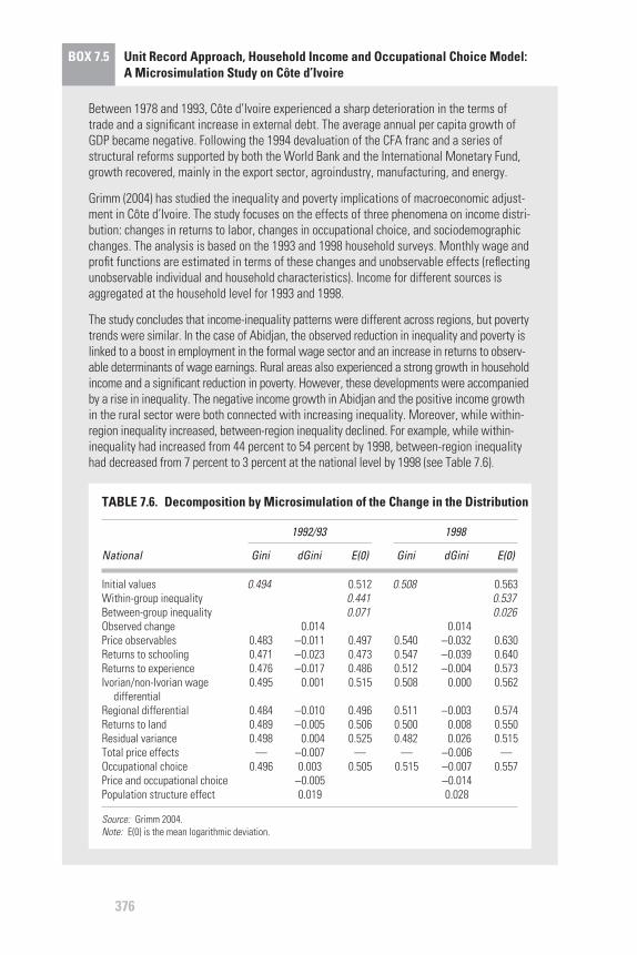
BOX 7.5 Unit Record Approach, Household Income and Occupational Choice Model: A Microsimulation Study on Côte d’Ivoire
Between 1978 and 1993, Côte d’Ivoire experienced a sharp deterioration in the terms oftrade and a significant increase in external debt. The average annual per capita growth ofGDP became negative. Following the 1994 devaluation of the CFA franc and a series ofstructural reforms supported by both the World Bank and the International Monetary Fund,growth recovered, mainly in the export sector, agroindustry, manufacturing, and energy.
Grimm (2004) has studied the inequality and poverty implications of macroeconomic adjust-ment in Côte d’Ivoire. The study focuses on the effects of three phenomena on income distri-bution: changes in returns to labor, changes in occupational choice, and sociodemographicchanges. The analysis is based on the 1993 and 1998 household surveys. Monthly wage andprofit functions are estimated in terms of these changes and unobservable effects (reflectingunobservable individual and household characteristics). Income for different sources isaggregated at the household level for 1993 and 1998.
The study concludes that income-inequality patterns were different across regions, but povertytrends were similar. In the case of Abidjan, the observed reduction in inequality and poverty islinked to a boost in employment in the formal wage sector and an increase in returns to observ-able determinants of wage earnings. Rural areas also experienced a strong growth in householdincome and a significant reduction in poverty. However, these developments were accompaniedby a rise in inequality. The negative income growth in Abidjan and the positive income growthin the rural sector were both connected with increasing inequality. Moreover, while within-region inequality increased, between-region inequality declined. For example, while within-inequality had increased from 44 percent to 54 percent by 1998, between-region inequalityhad decreased from 7 percent to 3 percent at the national level by 1998 (see Table 7.6).
TABLE 7.6. Decomposition by Microsimulation of the Change in the Distribution
1992/93 1998
National Gini dGini E(0) Gini dGini E(0)
Initial values 0.494 0.512 0.508 0.563Within-group inequality 0.441 0.537Between-group inequality 0.071 0.026Observed change 0.014 0.014Price observables 0.483 −0.011 0.497 0.540 −0.032 0.630Returns to schooling 0.471 −0.023 0.473 0.547 −0.039 0.640Returns to experience 0.476 −0.017 0.486 0.512 −0.004 0.573Ivorian/non-Ivorian wage 0.495 0.001 0.515 0.508 0.000 0.562
differentialRegional differential 0.484 −0.010 0.496 0.511 −0.003 0.574Returns to land 0.489 −0.005 0.506 0.500 0.008 0.550Residual variance 0.498 0.004 0.525 0.482 0.026 0.515Total price effects — −0.007 — — −0.006 —Occupational choice 0.496 0.003 0.505 0.515 −0.007 0.557Price and occupational choice −0.005 −0.014Population structure effect 0.019 0.028
Source: Grimm 2004.Note: E(0) is the mean logarithmic deviation.
shocks and policies on the key exogenous variables. General equilibriummodels can be used to introduce more structure in the analysis.
In this section, the logic of general equilibrium modeling is firstreviewed. Two ways of modeling distributional mechanisms are thenexamined based on two key sources: Dervis, de Melo, and Robinson (1982)and Decaluwé et al. (1999).
The logic of general equilibrium modeling
What is a general equilibrium model?
A general equilibrium model is a logical representation of a socioeconomicsystem wherein the behavior of all participants is compatible. The keymodeling issues thus entail the following: (1) the identification of the par-ticipants, (2) the specification of individual behavior, (3) the mode ofinteraction among socioeconomic agents, and (4) the characterization ofcompatibility.
The basic Walrasian framework serves as a template for most appliedgeneral equilibrium models. There are two basic categories of agents: con-sumers and producers, which are also referred to as households and firms.The behavior of each economic agent is supposed to conform to the opti-mization principle, which holds that the agent attempts to implement thebest feasible action. Thus, modeling optimizing behavior entails the speci-fication of (1) actions that an economic unit can undertake, (2) the con-straints it faces, and (3) the objective function used to evaluate such actions(Varian 1984). Within this framework, each household buys the bestbundle of commodities it can afford. The objective that guides householdchoice is therefore utility maximization, and the constraints are expressedin terms of budget constraints. Choices by a firm are characterized byprofit maximization, subject to technological and market constraints.
Households and firms are supposed to interact through a networkof perfectly competitive markets. Market interaction is a mode of socialcoordination through a mutual adjustment among participants based onquid pro quo (Lindblom 2001).6 Market participants are buyers andsellers whose supply and demand behavior is an observable consequenceof the optimization assumption. In this setting, behavioral compatibil-ity is described in terms of market equilibrium. General equilibrium isachieved by an incentive configuration (as represented through relativeprices) such that, for each market, the amount demanded is equal to theamount supplied. Alternatively, we can say that, when the economic sys-tem is in a state of general equilibrium, no feasible change in individualbehavior is worthwhile, and no desirable change is feasible.
Macroeconomic Shocks and Policies
377
Comparative statics entail a comparison of the equilibrium statesassociated with changes in the socioeconomic environment. Suchchanges may be induced by shocks or policy reforms. The comparisonof equilibrium states can be framed within a social evaluation. The eval-uation has two perspectives: individual and social. If one focuses onindividual objectives, then Pareto efficiency implies that no participantcan be made better off without making some other participant worseoff. A poverty-focused criterion would say that less poverty is preferableto more.
Empirical implementation
For policy analysis, one needs to move from a conceptual framework toa computable model. Applied general equilibrium models are commonlyrepresented by systems of equations. These equations fall into the fol-lowing basic categories: (1) demand equations from the optimizingbehavior of consumers, (2) supply equations from the optimizing behav-ior of firms, (3) income equations describing the income of each agentbased on prevailing prices and the quantities exchanged on goods andfactors markets, and (4) equilibrium conditions for all markets. All sup-ply and demand equations are homogeneous of degree zero. If one mul-tiplies all commodity and factor prices by a constant factor k, theequilibrium supply and demand will not change. Thus, the model ismoney neutral and can determine only relative prices. This creates theneed to normalize the price system by fixing a numéraire price. Themodel also satisfies Walras’ Law. Accordingly, if all economic agents sat-isfy their budget constraints and all but one of the markets are in equi-librium, then the last market must automatically be in equilibrium(Dinwiddy and Teal 1988).
The choice of the functional forms determines the set of structuralparameters that must be estimated to make the model computable. Thenecessary data usually come in the form of a social accounting matrix(SAM). The matrix reflects the circular flow of economic activity for thechosen year. It provides an analytically integrated data set that reflectsvarious aspects of the economy, such as production, consumption,trade, accumulation, and income distribution. A SAM is a square matrix,the dimension of which is determined by the institutional setting under-lying the economy under consideration. Each account is represented bya combination of one row and one column with the same label. Each entryrepresents a payment to a row account by a column account. Thus, all receipts into an account are read along the corresponding row, while
Analyzing the Distributional Impact of Reforms
378
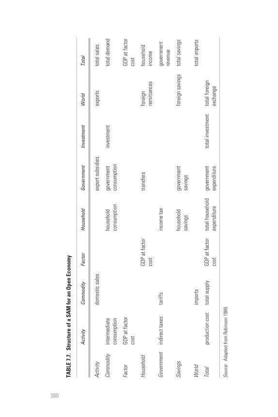
payments by the same account are recorded in the corresponding column.In accordance with the principles of double-entry bookkeeping, the wholeconstruct is subject to a consistency restriction that makes the columnsums equal to the corresponding row sums. This restriction also meansthat the SAM obeys Walras’ Law in the sense that, for an n-dimensionalmatrix, if the (n−1) accounts balance, so must the last one. Table 7.7 showsthe structure of a SAM for a model of an open economy.
For the purpose of analyzing the impact of macroeconomic shocksand policies on poverty and income distribution, it is important to under-stand how shocks and policies affect key macroeconomic balances before con-sidering how the repercussions are transmitted to households. In general, themacroeconomic properties of a static general equilibrium model of a realeconomy such as the one described here depend on the closure rule cho-sen. Such a rule refers to the equilibrating mechanisms governing prod-uct and factor markets, as well as the following three basic macrobalances:the balance of trade, the government budget balance, and the savings-investment balance. The inevitable inclusion of these macrobalances inthe basic Walrasian framework requires the specification of a correspond-ing flow equilibrium condition for which a closure rule has to be stated(Robinson and Löfgren 2005).
Robinson (2003) discusses four possible closures for this class ofmodels. Two of these assume the full employment of factors of produc-tion, while the other two do not. Assuming that output is a function of twofactors of production (capital and labor), there are 10 potential closurevariables: the GDP deflator, the wage rate, the exchange rate, investmentdemand, the trade balance, labor supply, the government consumptionof goods and services, capital, the savings rate, and the income tax rate.Closure rules differ on the basis of which three (the number of macrobal-ances in the model) of these 10 variables are made endogenous, while allthe rest are exogenous.
The first full-employment closure, also known as neoclassical, con-siders the wage rate, the exchange rate, and investment demand asendogenous variables. The second full-employment closure considersthe wage rate, the exchange rate, and the balance of trade as endogenous.Closure rules that assume unemployment are known as Keynesian. Thefirst rule makes the GDP deflator, the exchange rate, and labor supplyendogenous. For the second rule, the endogenous variables are the GDPdeflator, the trade balance, and labor supply. It is worth noting that theGDP deflator is a numéraire price in the full employment case, while thewage rate plays that role in the Keynesian case.
Macroeconomic Shocks and Policies
379
380
TAB
LE7.
7.St
ruct
ure
ofa
SAM
fora
nO
pen
Econ
omy
Activ
ityCo
mm
odity
Fact
orHo
useh
old
Gove
rnm
ent
Inve
stm
ent
Wor
ldTo
tal
Activ
ity
Com
mod
ity
Fact
or
Hous
ehol
d
Gove
rnm
ent
Savi
ngs
Wor
ld
Tota
l
dom
estic
sale
s
tarif
fs
impo
rts
tota
lsup
ply
GDP
atfa
ctor
cost
GDP
atfa
ctor
cost
hous
ehol
dco
nsum
ptio
n
inco
me
tax
hous
ehol
dsa
ving
s
tota
lhou
seho
ldex
pend
iture
expo
rtsu
bsid
ies
gove
rnm
ent
cons
umpt
ion
trans
fers
gove
rnm
ent
savi
ngs
gove
rnm
ent
expe
nditu
re
inve
stm
ent
tota
linv
estm
ent
expo
rts
fore
ign
rem
ittan
ces
fore
ign
savi
ngs
tota
lfor
eign
exch
ange
tota
lsal
es
tota
ldem
and
GDP
atfa
ctor
cost
hous
ehol
din
com
e
gove
rnm
ent
reve
nue
tota
lsav
ings
tota
lim
ports
Sour
ce:
Adap
ted
from
Robi
nson
1989
.
inte
rmed
iate
cons
umpt
ion
GDP
atfa
ctor
cost
indi
rect
taxe
s
prod
uctio
nco
st
A further examination of the neoclassical rule illustrates the types ofanalytical restrictions that such rules place on a general equilibriummodel for the purpose of macroeconomic analysis. This rule makes thecurrent account balance7 exogenous, along with savings rates and gov-ernment expenditure. Given that the current account balance is relatedto the functioning of the asset market, making it exogenous means thatthe corresponding flow of funds must be added to or subtracted fromthe savings-investment account (in the SAM). Equivalently, the budgetconstraint of at least one agent includes an exogenous net asset change(Robinson and Löfgren 2005). This closure rule leaves unexplained thedecision of households to save at fixed rates and the allocation by house-holds of savings across different assets.
With respect to the government account, it is commonly assumedthat government expenditure (both consumption and transfers) is fixedin real terms and that government revenue depends on fixed tax rates.The government deficit or surplus is computed residually and added tothe savings-investment account without any consideration of the specificfinancial mechanisms involved.
The above discussion clearly shows that a general equilibrium modelbased on this closure will certainly be useful in tackling the medium- tolong-term structural implications of a shock or a policy that works throughindividual markets, provided it is sufficiently disaggregated to account forpolicy-relevant sectors. The model, however, would have a limited abilityto deal with flow-of-funds issues related to the determination of aggregatesavings, the savings-investment balance, and the allocation of investmentacross the production sector. This requires the addition of financial mech-anisms to the general equilibrium model.
Robinson and Tyson (1984) offer an illustration through an exampleof a terms-of-trade shock and the interdependence between structuralissues that are essentially microeconomic in nature and aggregate flow-of-funds issues that are basically macroeconomic. They also suggest a frame-work for analyzing this interdependence and the implications for policytrade-offs and effectiveness. The basic idea is to link a proper macroeconomicmodel to a Walrasian general equilibrium model through variables that areendogenous in one, but exogenous in the other. For instance, a macromodelmay treat the price level and various macroeconomic aggregates, such asemployment, investment, and consumption, as endogenous. These vari-ables may then be specified as exogenous in the general equilibrium model.However, the closure rules for macrobalances and factor markets must bedesigned in such a way that the general equilibrium model behaves in amanner that is consistent with the outcome of the macromodel.
Macroeconomic Shocks and Policies
381

Modeling distributional mechanisms
Dervis, de Melo, and Robinson (1982) note that policymakers might beinterested in how income is distributed among the following: (1) factorsof production, (2) institutions, (3) socioeconomic groups, (4) house-holds, and (5) individuals. Distribution to factors of production is knownas functional distribution, while distribution to individuals is called sizedistribution. The choice of the Walrasian framework with a neoclassicalclosure focuses analysis on the microeconomic determinants of incomedistribution based on relative factor intensities in production and theinteraction among supply, demand, and employment.
A sufficiently disaggregated SAM provides a data framework formappings among various types of distributions of income. Referring backto Table 7.7, we note that the functional distribution of income is givenby the intersection of the factor-row and the activity-column. Depend-ing on data availability, this functional distribution can be disaggregatedby sector of production (agriculture, industry, and services) and by laborcategories if the labor market is segmented. When, in addition, factors ofproduction are disaggregated so that labor is differentiated by skill, edu-cation, or sector of employment and capital is differentiated by type, sec-tor, or region, we get what Löfgren, Robinson, and El-Said (2003) call theextended functional distribution of income.
GDP at market prices that includes indirect taxes is distributedamong various institutions such as households, enterprises, and govern-ment.8 Government revenue from all taxes is spent on export subsidies,government consumption, and transfers to households. The residual isput in the capital account. This framework does not explain various flowsof funds related to the activities of the central bank, such as money cre-ation or credit and interest rate policies. Therefore, it would be difficultto analyze the distributional implications of these macroeconomic poli-cies within this model. Both the functional and institutional distributionsclassify flows of funds according to the functional (factor employment)and institutional structure of the economy.
The household account in the SAM actually stands for all the peoplein the economy and may in fact cover all nongovernmental institutions,including enterprises. Thus, the distributions by socioeconomic groups,households, and individuals are various representations of the distribu-tion of income within this account (Dervis, de Melo, and Robinson 1982).The classification of individuals or households by socioeconomic group is dic-tated by policy issues and data availability. One simple scheme differenti-ates groups by type and source of income. Given an exhaustive andmutually exclusive partition of the entire population into socioeconomic
Analyzing the Distributional Impact of Reforms
382
groups, it is possible to derive the overall size distribution of income as aweighted sum of within-group density functions. Using the log varianceas an indicator of relative inequality, overall inequality can be decom-posed into within-group and between-group components. Thus, ceterisparibus, an increase in inequality in any one group or an increase in thedistance between one group’s average income and the overall meanincome will boost overall inequality. Given that the overall size distributionis derived empirically, one can compute any desired measure of inequalityor poverty (given a poverty line). In the simulation of the inequality impli-cations of shocks and policies, only between-group inequality can be generatedendogenously by this framework through changes in group means. This isbecause within-group distributions are exogenous.
The fact that the overall distribution of income is derived numericallyas a weighted sum of individual group distributions makes it possible toallow the functional form to vary from group to group. The lognormaldistribution that has often been used in this context is known to providea poor approximation of the distribution at the upper extreme. Onecould use the Pareto distribution for high-income groups. Employing adifferent function for every within-group distribution increases the abil-ity of the model to capture the heterogeneity of socioeconomic groups.Decaluwé et al. (1999) use the Beta distribution to this effect. This func-tion is fully characterized by the minimum income, the maximum income,and two shape parameters defining the skewness of the distribution. In amodel of an archetypical developing country, these authors allow the fourcharacteristic parameters of the Beta distribution to vary across six socio-economic groups: (1) landless rural households, (2) rural smallholders,(3) big landlords, (4) urban households with poorly educated heads,(5) urban households with highly educated heads, and (6) capitalists.9
Instead of aggregating group distributions into an overall distribution, theauthors compute, for each group, poverty measures of the Foster-Greer-Thorbecke family. Overall poverty can then be inferred as a weighted sumof within-group poverty whereby the weights are given by populationshares. Decaluwé et al. (1999) allow the nominal poverty line to be deter-mined within the model. The value of the reference basket of goods is adjustedon the basis of equilibrium prices computed by the model.
An application of the CGE model is shown in Box 7.6.The basic idea underlying the approach discussed here involves link-
ing an extended functional distribution to a size distribution of income.Various socioeconomic groups are considered as representative house-holds. This approach is thus called the extended representative household(ERH) approach to distinguish it from the standard representative house-
Macroeconomic Shocks and Policies
383
384
BOX 7.6 CGE Model: The Impact of Trade Policies on Income Distribution in a PlanningModel for Colombia
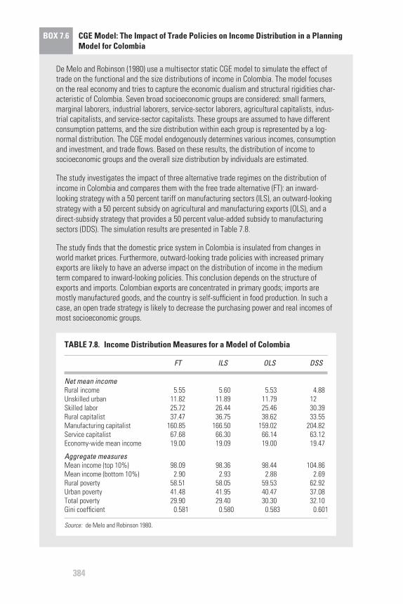
De Melo and Robinson (1980) use a multisector static CGE model to simulate the effect oftrade on the functional and the size distributions of income in Colombia. The model focuseson the real economy and tries to capture the economic dualism and structural rigidities char-acteristic of Colombia. Seven broad socioeconomic groups are considered: small farmers,marginal laborers, industrial laborers, service-sector laborers, agricultural capitalists, indus-trial capitalists, and service-sector capitalists. These groups are assumed to have differentconsumption patterns, and the size distribution within each group is represented by a log-normal distribution. The CGE model endogenously determines various incomes, consumptionand investment, and trade flows. Based on these results, the distribution of income tosocioeconomic groups and the overall size distribution by individuals are estimated.
The study investigates the impact of three alternative trade regimes on the distribution ofincome in Colombia and compares them with the free trade alternative (FT): an inward-looking strategy with a 50 percent tariff on manufacturing sectors (ILS), an outward-lookingstrategy with a 50 percent subsidy on agricultural and manufacturing exports (OLS), and adirect-subsidy strategy that provides a 50 percent value-added subsidy to manufacturingsectors (DDS). The simulation results are presented in Table 7.8.
The study finds that the domestic price system in Colombia is insulated from changes inworld market prices. Furthermore, outward-looking trade policies with increased primaryexports are likely to have an adverse impact on the distribution of income in the mediumterm compared to inward-looking policies. This conclusion depends on the structure ofexports and imports. Colombian exports are concentrated in primary goods; imports aremostly manufactured goods, and the country is self-sufficient in food production. In such acase, an open trade strategy is likely to decrease the purchasing power and real incomes ofmost socioeconomic groups.
TABLE 7.8. Income Distribution Measures for a Model of Colombia
FT ILS OLS DSS
Net mean incomeRural income 5.55 5.60 5.53 4.88Unskilled urban 11.82 11.89 11.79 12Skilled labor 25.72 26.44 25.46 30.39Rural capitalist 37.47 36.75 38.62 33.55Manufacturing capitalist 160.85 166.50 159.02 204.82Service capitalist 67.68 66.30 66.14 63.12Economy-wide mean income 19.00 19.09 19.00 19.47
Aggregate measuresMean income (top 10%) 98.09 98.36 98.44 104.86Mean income (bottom 10%) 2.90 2.93 2.88 2.69Rural poverty 58.51 58.05 59.53 62.92Urban poverty 41.48 41.95 40.47 37.08Total poverty 29.90 29.40 30.30 32.10Gini coefficient 0.581 0.580 0.583 0.601
Source: de Melo and Robinson 1980.
hold (RH) approach, which limits the analysis of the distributionalimpact of shocks and policies to their effects on representative socioeco-nomic groups. There is one other way of implementing the ERHapproach (discussed in Agénor, Chen, and Grimm 2004). The treatmentof the size distribution in this case is analogous to the approach underly-ing PovStat. Indeed, it is assumed that, following a shock or the imple-mentation of a policy, per capita consumption and disposable income fora household change at the same rate as the rate predicted by the generalequilibrium model for the socioeconomic group to which the householdbelongs.10 Thus, the size distribution is represented directly by relevantunit records from a household survey. Following a shock or the imple-mentation of a policy, a new distribution of income and consumption isgenerated by applying the predicted rates of change to the initial data.New measures of poverty and inequality can therefore be computed andcompared to baseline values.
This approach can only predict changes in between-group inequalitybecause the income and consumption of all the households belonging toa single socioeconomic group are scaled (up or down) by the same factor.Another limitation noted by the authors is the fact that the approach doesnot account for changes in the structure of employment. Therefore, theypropose an extension of the approach based on a reweighing procedurethat reassigns population weights to households in a manner that is con-sistent with predicted changes in the structure of employment.
LINKING A MACROECONOMIC FRAMEWORK TO A MODEL OF INCOME DISTRIBUTION
To be sure, both the standard RH and the ERH approaches reveal thebasic principles involved in linking a macroeconomic model to a repre-sentation of the distribution of economic welfare across individuals orhouseholds. This section focuses on some specific models (tools) that havebeen built more or less around these principles. The first one described isthe 123PRSP model, a three-layer and parsimonious framework designedto link macroeconomic policies to poverty outcomes via a two-sectorgeneral equilibrium model of an open economy.
Two implementations of the PAMS framework are then considered.The first interpretation of this framework uses the ERH approach basedon unit records to simulate the poverty impact of macroeconomic shocksand policies analyzed within a macroconsistency model such as the RevisedMinimum Standard Model Extended (RMSM-X). The second interpre-tation is a reduced form of the first, whereby a CGE model is linked
Macroeconomic Shocks and Policies
385

recursively (in a top-down fashion) to a poverty module built upon aparameterization of the Lorenz curve à la POVCAL.
A different macro-micro simulation model is then reviewed, whereinthe macroeconomy is represented by an IS-LM model.
Finally, the IMMPA framework is described briefly. The frameworklinks a dynamic CGE model including a financial sector to a distribu-tional module that is analogous to PovStat.
Given the distributional concerns, these models must ultimately be judgedon the basis of how well they use the wealth of available information (fromnational accounts and household surveys) to explain the interdependenceamong sectors and institutions and the heterogeneity of actors. Naturally, ina particular environment, additional criteria come into play, such as theskills required of the analyst in implementing a given approach.
The 123PRSP model
The 123PRSP model is based on the idea that the impact on poverty ofmacroeconomic shocks and policies is transmitted through two basicchannels. The first channel involves distributional-neutral changes in theaverage income, while the second is the change in the sectoral pattern ofgrowth induced by changes in relative prices (for example, shifts in the realexchange rate). The overall impact is thus equal to the pure growthimpact, plus the distributional impact.
This idea is implemented within a three-layer model. The macrolayerhas three components: (1) a financial programming model, (2) a trivariatevector autoregressive (VAR) model, and (3) a medium-term growthmodel based on cross-country regression analysis. The meso- (or inter-mediate) layer is represented by a two-sector general equilibrium modelof an open economy. Finally, the microlayer relies on the envelope theo-rem to model the distribution of welfare across households.
The financial programming module
Generally speaking, financial programming is the process of designinga consistent set of macroeconomic policies, whereby instruments (forexample, domestic credit) are set in such a way that a target variable(official reserves, for instance) follows a desired trajectory. In the contextof policy reform programs supported by the International Monetary Fund,this approach is used to set monetary and fiscal policies aimed at restrainingaggregate demand and adjusting relative prices. Financial programmingcan be described in terms of the underlying accounting framework thatimposes consistency upon data and any prediction based on assumed
Analyzing the Distributional Impact of Reforms
386

behavioral relationships or projection rules.11 The approach emphasizesthe monetary dimension of the balance of payments and relates themonetary and fiscal accounts to the balance of payments.
The economy is divided into four institutional sectors: (1) the pri-vate sector, (2) the public (government) sector, (3) the foreign sector orthe rest of the world, and (4) the domestic banking sector. Each sectorin the economy is represented by a budget that constrains its behavior,and all variables are measured in nominal local currency. Within thisframework, financial transactions are distinguished from those arisingfrom the production or acquisition of goods and services (also knownas income/expenditure transactions). It is assumed that the private sectorowns all factors of production. The private sector gets nominal incomefrom the sale of current output. This income is used to pay taxes to thegovernment, purchase goods for consumption, and make investments.Any disposable income after expenditure is used to accumulate financialassets or liabilities in the form of money, foreign assets, and borrowingfrom the banking system.
The public sector collects taxes from the private sector and uses theproceeds for consumption. Any surplus or deficit is accounted for by theaccumulation of financial assets or liabilities in the form of foreign assetsand net borrowing from the banking system. The foreign sector gets rev-enues from the sale of imports to the domestic economy. It spends ondomestic exports. In the case of a current account deficit, the revenues ofthe foreign sector exceed its expenditures. The foreign sector can buy backits liabilities from the domestic private and public sectors and acquiresreserves from the domestic banking system. The financial sector func-tions as a financial intermediary among various actors. It obtains assetsin the form of international reserves and claims on domestic actors andissues its own liabilities in the form of money to the private sector.
These budget constraints are not independent; they represent anoverall resource constraint on the economy. This resource constraint canbe expressed as follows: the difference between gross national disposableincome and domestic absorption is equal to the current account balance.12
The linkages among these sectoral accounts imply that a deficit in anysector must be financed by savings in other sectors. For the whole econ-omy, excess spending is possible only if financing is available from therest of the world. The relationship between excess absorption and thecurrent account balance shows that an improvement in the latter may beachieved through an increase in the country’s output or a reduction inabsorption. Furthermore, the sum of the current account balance and netcapital inflows is equal to the change in net official reserves. This identity
Macroeconomic Shocks and Policies
387

connects excess absorption (over income) to two financing sources: cap-ital inflows to the nonbanking sector and official international reserves.This clearly shows that the current account balance acts as a resourceconstraint on the whole economy (IMF 1987).
The basic structure of the financial programming model can beunderstood by focusing on the case of a small open economy with a fixedexchange rate, which is known as the Polak model (Agénor 2004a; Polak1998; IMF 1987). In this context, the money supply is viewed as anendogenous variable that depends on changes in the balance of payments.
The core model contains four relationships. The first relationship isan accounting identity based on the balance sheet of the banking system.13
Accordingly, the change in the money supply (a liability for the bankingsystem) equals the sum of the change in net official reserves and thechange in net domestic credit (that is, the sum of changes in the foreignand domestic assets held by the banking system). The second relationshipdefines the change in the nominal demand for money as the change in thenominal income multiplied by the inverse of the income velocity ofmoney, which is assumed to be constant over time. The third relation-ship defines flow equilibrium in the money market. The last relationshiprestates the balance of payments identity as follows: the change in officialreserves is equal to exports, minus imports, plus the change in net capi-tal inflows to the nonbanking system. Exports are assumed to be exoge-nous, while imports are computed as national income multiplied by aconstant marginal propensity to import.
The design of a financial program involves an iterative processbased on the following five steps (IMF 1987): (1) Set the target for thechange in the official reserves. (2) Use the last relationship (the balanceof payments identity) to compute residually a value for imports that isconsistent with the reserve target and the assumed level of the exoge-nous variables (exports and the change in net capital flows to the non-banking sector). (3) Project nominal income and use the projection,along with the assumed values for the income velocity of money and themarginal propensity to import, to obtain the demands for money andimports. (4) Given a forecast of the money demand (equal to the moneysupply in equilibrium) and the target for official reserves, use the balance-sheet identity of the banking system (first equation) to infer thechange in domestic credit that is compatible with the target for officialreserves and the desired increase in nominal money balances. (5) Checkfor consistency by comparing the projected imports with the residualvalue computed from the balance of payments identity in step 2. If thetwo values are equal, stop the process; if not, make adjustments to the
Analyzing the Distributional Impact of Reforms
388
underlying assumptions and repeat the process until consistency isachieved.
Monetary and fiscal policy can be linked through the financial pro-gramming framework by distinguishing the expansion of credit to theprivate sector from that to the public sector (IMF 1987). Thus, the totalchange in the domestic assets of the banking system appearing in thebalance-sheet identity must now include two components: (1) the changein domestic credit to the government and (2) the change in domesticcredit to the private sector. Similarly, the total change in foreign capitalinflows to the nonbanking sector has two components: public and pri-vate. Finally, a relationship must be added to reflect the fact that the gov-ernment can finance its budget deficit through net borrowing either fromabroad or from the domestic banking system.
The growth module
The growth module has two components. The first is a trivariate VARmodel designed to capture an improvement or deterioration in the termsof trade or other short-run growth impact that is produced by a shock ora change in government expenditure or other short-run growth impactthat is produced by a policy reform. The VAR model is a useful tool foranalyzing interrelationships among different time series. In this frame-work, all variables are endogenous because of the assumption that the timepath of each variable affects and is affected by current and past realizationsof the other variables. A VAR model may be characterized by the numberof variables (time series) and the longest lag length (Enders 1995). Thus,a first-order bivariate VAR would involve two variables and a lag lengthof at most one. The random disturbances in the VAR framework areknown as innovations or shocks. A shock in one variable not only affectsthat variable directly, but is also transmitted to all the other variables,depending on the lag structure of the model. A VAR can be written as avector moving-average of the shocks, from which one can derive impulseresponse functions. An impulse response function represents the behaviorof time series in response to various shocks. The 123PRSP frameworkincludes the following three variables: the growth rate, the real exchangerate, and either the terms of trade or government expenditure. The param-eter estimates based on impulse response functions are interpreted as short-run growth elasticities.
The second component of the growth module is a cross-countryregression model (Easterly 2001) designed to capture the impact of macro-economic policies on long-run growth. The model involves three groupsof independent variables. The first group includes policy determinants of
Macroeconomic Shocks and Policies
389
growth: (1) a black market premium, (2) a measure of financial devel-opment (M2/GDP),14 (3) inflation, (4) the real exchange rate, (5) secon-dary education enrollment, and (6) telephone lines per 1,000 individuals(a proxy for infrastructure stock). The second group of variables capturesthe impact of shocks such as: (1) the terms of trade as a percentage of GDP,(2) the interest on external debt as a percentage of GDP, and (3) growthamong trading partners of the Organisation for Economic Co-operationand Development. Finally, variables measuring initial conditions include(1) initial income, (2) an intercept, (3) a dummy variable for the 1980s,and (4) a dummy variable for the 1990s.
The two-sector general equilibrium model
The mesolayer of the 123PRSP is represented by a two-sector generalequilibrium model of a small open economy. The model is a generaliza-tion of the Salter-Swan framework, which provides a foundation for thestudy of the impact of macroeconomic imbalances and adjustmentpolicies on the real sector of the economy. This single-country model(as opposed to a multicountry trade model) represents a significantimprovement on both the standard neoclassical trade model and theSalter-Swan model. The neoclassical model often leads to implausibleempirical results because of two basic assumptions. The first assumptionstates that all goods are tradable, while the second implies perfect substi-tutability between foreign and domestic goods. These two assumptionsimply the law of one price, according to which the domestic prices oftradable goods and services are determined by the world market.
The Salter-Swan framework makes an important distinction betweentradable and nontradable goods and services. Nontradables are goods andservices the prices of which are determined by supply and demand con-ditions within domestic markets. Prices for tradable goods are deter-mined by the world market. The fact that a good is nontradable may bedue to its nature (such as public services or construction) or to prohibi-tive transport costs that keep the good off the world market. Thus, somepolicy changes may cause some goods to switch categories. Further-more, the country under consideration is assumed to be small withrespect to international trade and therefore faces a perfectly elasticexcess supply from the rest of the world. In other words, it cannot affectthe terms at which it is trading with the rest of the world. Exportableand importable goods can therefore be aggregated into a single class ofgood, tradables, using world prices as weights. The model still main-tains the neoclassical assumption that domestic and foreign goods areperfect substitutes in consumption and focuses on the effects of external
Analyzing the Distributional Impact of Reforms
390
shocks on the real exchange rate, which ultimately directs resource allo-cation within the economy.
The extensions of this framework as implemented within the 123PRSPdrop the assumptions about aggregation and perfect substitution andexplicitly add government, savings, and investment.15 These extensionsallow the inclusion of policy instruments such as taxes, as well as the con-sideration of macroeconomic effects. These extensions are now brieflydescribed. (See Devarajan, Lewis, and Robinson 1990 for a more detailedpresentation.)
The small country assumption is maintained; thus, the country can-not affect its terms of trade with the rest of the world. There are two sec-tors of production. The first produces exports, and the second producesall other final goods, which are referred to as domestic (home) goods.Real GDP is an aggregation of exports and domestic goods based on aconstant elasticity of transformation function.16 The supply of exportsrelative to domestic goods is obtained by maximizing GDP, subject to thetechnical transformability constraint (above) and sales opportunities athome and abroad.
Consumption is expressed in terms of a composite good that is anaggregation of home goods and imports based on a constant elasticity ofsubstitution function. The demand for imports and for domestic goodsis derived by minimizing the cost of the composite good, subject to a substi-tutability constraint represented by the elasticity of substitution function.The representative household is assumed to save a constant fraction of itsdisposable income. Gross income is the sum of GDP, transfers from thepublic sector, and remittances from abroad.
The domestic prices of exports and imports are calculated from worldprices, the exchange rate, and all applicable taxes. The GDP deflator is aweighted average of the domestic price of exports and that of home goods.The weights are the shares of each commodity in GDP. Similarly, theaggregate price of the composite consumption good is a weighted averageof the domestic prices of imports and home goods.
Two types of equilibrium conditions are explicitly stated. The firstgroup concerns commodity market equilibrium: (1) the supply of homegoods equals the demand, and (2) the supply of the composite good equalsthe demand, which includes private consumption, investment, andgovernment consumption (assumed to be fixed in real terms). The othergroup of conditions pertains to macroeconomic balances: (1) the currentaccount balance is fixed; (2) total savings (the sum of private, public, andforeign savings) equals investment, and (3) government revenue fromdirect and indirect taxes is accounted for by government consumption,
Macroeconomic Shocks and Policies
391
transfers, and savings. There are also implicit equilibrium conditions asso-ciated with the use of the constant elasticity of transformation production-possibility frontier. This assumption is a cover for the operation of factormarkets (labor and capital). Indeed, it is equivalent to assuming fullemployment in a single labor market within the economy. In this staticmodel, capital is assumed to be fixed and sector specific. Thus, there isan equilibrium wage rate associated with each equilibrium price forhome goods. Returns to capital in each sector can be computed residuallyfrom the value of output.
The financial programming model and the growth module trace themacroeconomic implications of shocks and policies. In particular, thesetwo submodules produce information on the evolution of GDP that isconsistent with the underlying macroeconomic framework over the rel-evant horizon. The 1-2-3 model then takes this information and com-putes the structural implications induced by a change in relative prices.This is a key link in the chain of transmission from macroeconomicevents to poverty. Based on the distinction between tradable and non-tradable commodities, the real exchange rate is defined as the price oftradables relative to nontradable goods. An increase in domestic pricesrelative to world prices is known as an appreciation of the real exchangerate, while a decrease marks a depreciation. Real appreciation of theexchange rate, for instance, shifts incentives in favor of domestic goodsrelative to exports. The final outcome depends on the structural charac-teristics of the economy as revealed by the elasticity of transformationand of substitution.
The microlayer
The purpose of the microlayer is to translate the solution of the 1-2-3general equilibrium model into changes in household welfare. For anymacroeconomic event worked out within the macroeconomic frame-work, the general equilibrium model computes the corresponding changesin income (wages and profit) by sector (tradable and nontradable) andthe changes in commodity prices (imports and home goods). The con-struction of the household module follows the envelope approach (dis-cussed elsewhere above). Here, the indirect utility is a function of the wagerate, sectoral profits, and commodity prices. These are the linkage variablesbetween the meso- and the microlayers. Thus, the first-order approxi-mation of the welfare impact of a macroshock at the household level isequal to the sum of three components: (1) the initial level of laborincome multiplied by the relative change in the wage rate, (2) the changein profit income, and (3) the sum over commodities of the product of
Analyzing the Distributional Impact of Reforms
392
the negative of the initial consumption and the relative change in thecommodity price.17
For the empirical implementation, distributions of income and expen-diture by deciles are derived from available household-survey data. Thereare three income sources: wages, profits from the home goods sector, andprofits from the exports sector. Consumption expenditure is dividedbetween imports and domestic goods. Heterogeneity among households isthus reflected by differences in the sources of incomes and in the patterns ofconsumption. This helps capture the differential impacts among house-holds of shocks and policies.
Consider, for instance, a cut in public expenditure that falls mainly onnontradable goods. If there is sufficient structural flexibility, the inducedfall in the price of nontradables will lead to a real depreciation in theexchange rate. The production of tradable goods will increase, while thatof nontradables will decline. The welfare impact at the household levelwill depend on whether a household is a net seller or a net buyer of trad-able goods. Net sellers would gain, while net buyers would lose. Once thesedifferential impacts are computed, standard techniques can be used toderive the desired poverty and inequality measures. However, it is impor-tant to keep in mind that, even when abundant and relevant household-leveldata are available, the ability of a modular framework such as 123PRSP toaccount for heterogeneity is constrained by the degree of disaggregation atthe mesolevel. By unifying the labor market and dividing the economyinto only two sectors, the 123PRSP model achieves a great deal of trans-parency at a significant cost in terms of heterogeneity.18
The use of the 123PRSP model is illustrated in Box 7.7.
Macroeconomic Shocks and Policies
393
BOX 7.7 The 123PRSP Model: Distributional Effects of Macropolicies and Shocks in Zambia
Devarajan and Go (2003) employ the 123PRSP model to examine the distributional impact ofmacroeconomic shocks and policies in Zambia.
Zambia is a landlocked economy that depends heavily on mineral exports, particularly copper.This renders the country very vulnerable to external price shocks. Over the 2001–3 period,two risk factors threatened macroeconomic stability in Zambia. The first shock stemmed fromexpenditure pressures associated with the presidential election in late 2001, and the secondfrom the decline in the world price of copper (the major export for the economy) induced by aslowdown in world demand.
(continued)
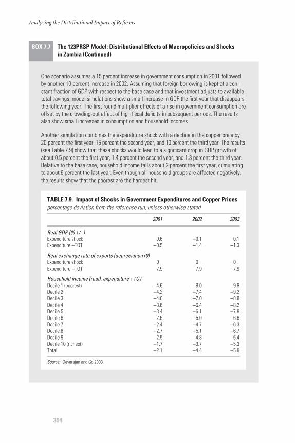
Analyzing the Distributional Impact of Reforms
394
BOX 7.7 The 123PRSP Model: Distributional Effects of Macropolicies and Shocks in Zambia (Continued)
One scenario assumes a 15 percent increase in government consumption in 2001 followedby another 10 percent increase in 2002. Assuming that foreign borrowing is kept at a con-stant fraction of GDP with respect to the base case and that investment adjusts to availabletotal savings, model simulations show a small increase in GDP the first year that disappearsthe following year. The first-round multiplier effects of a rise in government consumption areoffset by the crowding-out effect of high fiscal deficits in subsequent periods. The resultsalso show small increases in consumption and household incomes.
Another simulation combines the expenditure shock with a decline in the copper price by20 percent the first year, 15 percent the second year, and 10 percent the third year. The results(see Table 7.9) show that these shocks would lead to a significant drop in GDP growth ofabout 0.5 percent the first year, 1.4 percent the second year, and 1.3 percent the third year.Relative to the base case, household income falls about 2 percent the first year, cumulatingto about 6 percent the last year. Even though all household groups are affected negatively,the results show that the poorest are the hardest hit.
TABLE 7.9. Impact of Shocks in Government Expenditures and Copper Pricespercentage deviation from the reference run, unless otherwise stated
2001 2002 2003
Real GDP (% +/−)Expenditure shock 0.6 −0.1 0.1Expenditure +TOT −0.5 −1.4 −1.3
Real exchange rate of exports (depreciation>0)Expenditure shock 0 0 0Expenditure +TOT 7.9 7.9 7.9
Household income (real), expenditure +TOTDecile 1 (poorest) −4.6 −8.0 −9.8Decile 2 −4.2 −7.4 −9.2Decile 3 −4.0 −7.0 −8.8Decile 4 −3.6 −6.4 −8.2Decile 5 −3.4 −6.1 −7.8Decile 6 −2.6 −5.0 −6.6Decile 7 −2.4 −4.7 −6.3Decile 8 −2.7 −5.1 −6.7Decile 9 −2.5 −4.8 −6.4Decile 10 (richest) −1.7 −3.7 −5.3Total −2.1 −4.4 −5.8
Source: Devarajan and Go 2003.
The PAMS framework
PAMS is a simple simulation framework analogous to the 123PRSP to theextent that it is designed to help trace sequentially, in a top-down fashion,the poverty and distributional implications of macroeconomic shocks orpolicies. The original implementation of this framework (PAMS I) hasthree layers. The macroeconomic layer is represented by a standard macro-consistency model such as the World Bank’s RMSM-X.
The second layer, which represents the mesolevel of analysis, is basedon the idea that each household in the economy gets its means of liveli-hood both from the government (net public transfers) and from the mar-ket. The microlayer deals with household-level information organized onthe basis of policy-relevant characteristics in a way that allows easy linkageswith the mesoframework. Unit record data are used in a manner analo-gous to PovStat. The second generation of the framework is a reduced-form application that combines the macro- and mesolayers into a generalequilibrium model and employs a parameterization of the Lorenz curvefor poverty simulation.
This section first discusses the macroeconomic module within theRMSM-X framework. It then provides a brief description of the meso-module and the poverty simulator. It closes with a brief description of theessential features of the reduced-form version, which links a CGE modelto a parameterized Lorenz curve.
The RMSM-X module
In essence, the RMSM-X framework may be viewed as an extension of afinancial programming model that includes a growth model specified alongthe lines of the Harrod-Domar model.19 In the basic formulation, there arefour economic agents or sectors in the economy: (1) the central govern-ment, (2) the monetary system, (3) the private sector, and (4) the rest ofthe world (or the foreign sector). The underlying macroeconomic account-ing framework is the same as the one described in the section on financialprogramming. It obeys the principles of flow-of-funds accounting: (1) asource of funds for one sector represents a use of funds by another sector,and (2) for each sector, the total amount of funds from all sources mustequal the total disposition for all uses.
The structure of the model is characterized by (1) the budget con-straints facing each sector and the overall economy, (2) market equilibriumconditions for goods and asset markets, and (3) behavioral and projec-tion rules linking some variables to others. Consider, in particular, aneconomy with the four sectors and three assets above, including money,domestic lending by the banking system, and foreign debt.20 A basic
Macroeconomic Shocks and Policies
395

RMSM-X model could then be specified along the following lines. Thegrowth equation establishes a relationship among the growth of real out-put, investment, and the incremental capital output ratio (ICOR). Astandard assumption is that the ICOR is constant over time, whichimplies a proportional relationship between growth and investment.21
Next, one includes two equations describing changes in nominal outputand changes in the overall price index. The change in the overall priceindex can be defined as a weighted average of the changes in the index ofdomestic prices and the changes in the exchange rate.
On the financial side of the economy, one would add the followingrelationships from the financial programming framework. A money supplyequation would be derived from the balance sheet of the banking system.The equilibrium condition in the domestic lending market states that achange in domestic credit is the sum of the credit to the private sector andthe credit to the public sector. The credit to the private sector could beexpressed as a function of the change in nominal GDP. The change inofficial reserves is derived from the balance of payments identity. In thisidentity, exports are exogenous and computed on the basis of a simpleprojection rule. Imports can be computed as a function of real income andthe real exchange rate (Agénor 2004a). The flow of foreign debt is given bythe equilibrium condition on the foreign asset market, which states that thetotal flow is equal to the sum of the private and public flows. As before, thedemand for money is a function of the velocity parameter and nominalincome. Flow equilibrium prevails in the money market.
The budget constraints of both the public and private sectors canbe written in a reduced form that shows the accumulation of the assetsand liabilities associated with a surplus or deficit. In addition, to computeinvestment, the budget constraint of the private sector can be combinedwith the notion that private consumption is a linear function of dispos-able income (Agénor 2004a).
Adding up the four budget constraints in the model gives the fun-damental national income identity. The model therefore contains eightcore equations represented by the four budget constraints, the derivednational income identity, and the three flow equilibrium conditions inasset markets (money, domestic credit, and foreign debt). These coreequations are not mathematically independent due to the relationshipbetween the sectoral budgets and the overall resource constraint. The sys-tem thus obeys Walras’ Law and can be solved on the basis of only sevenof the core equations. The solution of the remaining equation can beinferred from that of the other seven. However, the solution proceduredepends on the closures chosen. There are three common closure rules
Analyzing the Distributional Impact of Reforms
396
(World Bank 1995). In the case of public closure, one seeks values of gov-ernment consumption and borrowing from both the monetary systemand abroad that are consistent with projected growth, inflation, and othervariables. In the case of private closure, one seeks a solution in terms ofprivate consumption and borrowing. With respect to the policy closure,one is interested in the likely impact of alternative macroeconomic pro-grams on target variables such as growth and inflation.
The policy closure seems more appropriate when the module isused to study the impact of macroeconomic policies on poverty and thedistribution of income. In this context, one could solve the systemrecursively as follows (World Bank 1995). Step 1: identify and fix all for-eign borrowing available to the country; then compute imports resid-ually from the balance of payments. Step 2: use the value of importsderived from step one in the national income identity to solve for pri-vate investment.22 Step 3: compute the value of the second target variable,the current price, from the money market equilibrium and the moneydemand equation.23 Step 4: derive total domestic credit residually from themoney supply equation. Step 5: given the change in government credit,compute private credit residually from the equilibrium condition of thedomestic credit market.
The mesomodule
The main element of this component is the labor and wage-incomemodule, which reconfigures the productive sector of the economy intoa number of sectors equal to the number of socioeconomic groups. Thiseffectively leads to a segmented labor market in the module. This seg-mentation is achieved as follows. First, the module divides the economyinto two basic components, rural and urban. Then, within each compo-nent, one distinguishes the formal sector from the informal sector. Withineach of these sectors, subsectors producing tradables are distinguishedfrom those producing nontradables.
GDP, which is determined at the macro level, is an important linkagevariable and must also be broken down according to the above categories.Here again, it will be necessary to determine residually the production ofcertain sectors (for example, the urban informal sector and the rural sub-sistence sector) in order to maintain overall consistency. The simplestway to model the rural economy is to represent its output as a constantelasticity function of rural labor. Within the urban economy, the produc-tion of the public sector is exogenous. Assuming that all private invest-ment in the economy occurs within the formal sector, the output in thatsector can be computed on the basis of an appropriate incremental cap-
Macroeconomic Shocks and Policies
397

ital output ratio. In such a case, the growth rate of output in the urbanformal economy would stand in a fixed-coefficient relationship with theratio of investment to output. For the sake of consistency, the output ofthe informal nontradable sector is determined residually.
Labor supply is seen as largely driven by demographic considera-tions and semi-exogenous migrations of labor and skill categories. Labordemand is broken down by socioeconomic categories, skill levels, andlocation (rural and urban) and is viewed as dependent on sectoral demand(output growth), as well as real wages. Hence, the new module determineswage income broken down by socioeconomic categories, skill levels, andlocation (rural and urban). Even though each sector in the reconfiguredeconomy may employ both skilled and unskilled labor, the module relieson a simplifying assumption according to which each sector employsonly one kind of labor. Thus, there is no substitution among types oflabor in the production process except for semi-exogenous migrationbased on the Harris-Todaro process.
The excess of the total income generated in the economy with respectto the total wage bill distributed to all labor categories represents the prof-its that are distributed to a representative class of rentiers. The currentversion of the tool does not track down financial assets and returns onthese assets. However, the interest revenue can conceivably be redistrib-uted from the macroframework to various socioeconomic groups accord-ing to some rule. Average tax and transfer rates are used to compute thedisposable income for each socioeconomic group. It is the percentagechange in this disposable income that is transmitted to the poverty sim-ulator in order to simulate the impact of shocks and policies on povertyand between-group inequality.
The poverty simulator
The poverty simulator in this version of PAMS (PAMS I) is analogous toPovStat. Intragroup distributions are represented by unit records per-taining to each socioeconomic group. To compute the impact of amacroeconomic shock or a policy on the welfare of a given household, theper capita income or expenditure of the household is multiplied by theinduced growth rate of the disposable income of the representative groupto which the household belongs. This growth rate is jointly determinedby the macro- and the mesolayers.
As with any of the frameworks examined here, there are structuraland, possibly, data constraints that can limit the reliability of the frame-work in predicting the poverty and distributional impact of macro-economic shocks and policies. In the particular case of PAMS I, there is
Analyzing the Distributional Impact of Reforms
398

a data constraint stemming from the fact that most household surveysprovide some information at the household level, such as expenditureand self-employment income, while other information, such as laborincome and employment status, is given at the individual level. Choos-ing the household as the unit of analysis means that individual-level datamust be aggregated up to the household level. Socioeconomic groups arethus created on the basis of the characteristics of heads of household. Thisobviously leads to results that are coarser than results based on relevantindividual-level data.
In addition, the poverty simulator is bound to inherit the strengthsand weaknesses of the top layers. It is well known, for instance, that thebasic RMSM-X is a simple macroeconomic accounting framework andshows no behavioral relationships in the economic sense. Also, the useof a labor demand function that is defined by sector and skill level isequivalent to assuming a homogenous labor factor with different, sector-specific remuneration.
Operational support
PAMS I has seen battle in support of the design of Poverty ReductionSupport Credits and the Poverty Assessment for Burkina Faso. Specifi-cally, the framework was used to simulate the poverty implications of nega-tive shocks to the cotton sector, as well as the impact of some patternsof growth. Assuming a permanent 20 percent decline in the price of cot-ton starting in 2004, the simulations reveal an increase of about 1.5 per-centage points above the baseline. Naturally, cotton farmers (18 percentof the population) are the most affected. This impact would be exacer-bated if it were accompanied by drop of 20 percent in output.
In the context of the analysis of the implications of different growthpatterns, the simulation framework was used to study the impact of shocksto the agriculture sector outside cotton. A 20 percent increase in the out-put of the primary sector could lead to a 3 percentage point decline inpoverty. One set of simulations concerns the implications of a pattern ofgrowth wherein the overall growth rate remains unchanged, while theprimary sector grows at a rate 2 percent higher than the baseline, alongwith a lower growth rate for the tertiary sector. In this case, poverty fallsby 1 percent up to 2007 and by 4 percentage points by 2015.
Reduced-form implementation
The purpose of the mesolayer in the original PAMS is to model an extendedfunctional distribution of the income generated by the upper-layer macro-economic model based on the selected socioeconomic groups. In practice,
Macroeconomic Shocks and Policies
399
several iterations are required in order to calibrate this module to availabledata. If a disaggregated SAM is available that is compatible with the selectedsocioeconomic groups, then it might be easier to compress the macro- andmesolayers into a general equilibrium model. As far as the poverty simula-tor is concerned, it should be noted that multiplying each observation(expenditure or income) in the unit record representation of a distributionby a scalar implies that the mean of the distribution is multiplied by thesame scalar. Given that the within-group group distribution remains con-stant from one state to another, one might as well construct the povertysimulator on the basis of group means and Lorenz functions estimatedfrom the available household data.
An example of the application of PAMS is supplied in Box 7.8.This approach increases computational efficiency in a simulation
environment. Thus, within the reduced-form version of PAMS (PAMS II)that runs in EViews (version 4.1 or later), poverty and distributionaloutcomes of shocks and policies are derived by linking recursively an appropriately disaggregated CGE model with a poverty and in-equality simulator built upon a parameterization of the Lorenz curve.The approach underlying PAMS II is analogous to the ERH approachdescribed elsewhere above. The main difference with other implemen-tations of this approach stems from the fact that, in the PAMS frame-work, the within-group size distribution of income is derived from theassumed Lorenz distribution. Many other applications assume func-tional forms for the density function characterizing the within-groupdistribution.
A macro-micro simulation model for Brazil
In the context of this review, a macro-micro simulation model stands forany simulation framework that links in some fashion a representation ofthe macroeconomy to a model of the size distribution of income. In thisfundamental sense, the 123PRSP model, PAMS, and even the ERH frame-work are members of the family of macro-micro simulation models. Twoapproaches commonly followed in the literature are to combine a CGEmodel either with an envelope model of welfare distribution or with anincome and occupational model. The first approach is analogous to theway 123PRSP links a two-sector CGE model to the corresponding house-hold module. Given this analogy and the fact that this chapter has alreadyreviewed the structure of CGE models and income-occupational models,the focus here below is only on an approach followed by Ferreira et al.(2004) in a study of the distributional impacts of macroeconomic shocks
Analyzing the Distributional Impact of Reforms
400
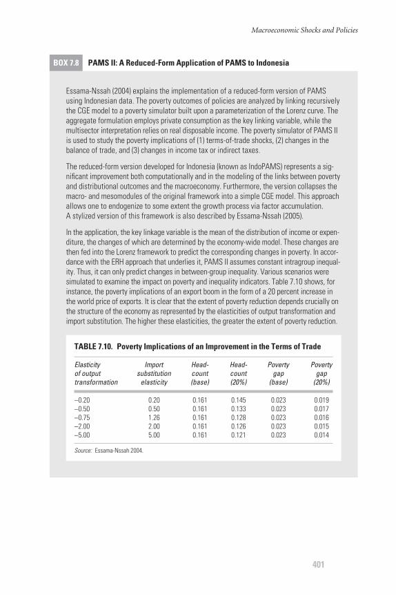
Macroeconomic Shocks and Policies
401
BOX 7.8 PAMS II: A Reduced-Form Application of PAMS to Indonesia
Essama-Nssah (2004) explains the implementation of a reduced-form version of PAMSusing Indonesian data. The poverty outcomes of policies are analyzed by linking recursivelythe CGE model to a poverty simulator built upon a parameterization of the Lorenz curve. Theaggregate formulation employs private consumption as the key linking variable, while themultisector interpretation relies on real disposable income. The poverty simulator of PAMS IIis used to study the poverty implications of (1) terms-of-trade shocks, (2) changes in thebalance of trade, and (3) changes in income tax or indirect taxes.
The reduced-form version developed for Indonesia (known as IndoPAMS) represents a sig-nificant improvement both computationally and in the modeling of the links between povertyand distributional outcomes and the macroeconomy. Furthermore, the version collapses themacro- and mesomodules of the original framework into a simple CGE model. This approachallows one to endogenize to some extent the growth process via factor accumulation. A stylized version of this framework is also described by Essama-Nssah (2005).
In the application, the key linkage variable is the mean of the distribution of income or expen-diture, the changes of which are determined by the economy-wide model. These changes arethen fed into the Lorenz framework to predict the corresponding changes in poverty. In accor-dance with the ERH approach that underlies it, PAMS II assumes constant intragroup inequal-ity. Thus, it can only predict changes in between-group inequality. Various scenarios weresimulated to examine the impact on poverty and inequality indicators. Table 7.10 shows, forinstance, the poverty implications of an export boom in the form of a 20 percent increase inthe world price of exports. It is clear that the extent of poverty reduction depends crucially onthe structure of the economy as represented by the elasticities of output transformation andimport substitution. The higher these elasticities, the greater the extent of poverty reduction.
TABLE 7.10. Poverty Implications of an Improvement in the Terms of Trade
Elasticity Import Head- Head- Poverty Poverty of output substitution count count gap gaptransformation elasticity (base) (20%) (base) (20%)
−0.20 0.20 0.161 0.145 0.023 0.019−0.50 0.50 0.161 0.133 0.023 0.017−0.75 1.26 0.161 0.128 0.023 0.016−2.00 2.00 0.161 0.126 0.023 0.015−5.00 5.00 0.161 0.121 0.023 0.014
Source: Essama-Nssah 2004.
in Brazil. They link an IS-LM model to a model of income and occupa-tional choice. In what follows, only the macroeconomic model and thelinkage variables are considered.
The IS-LM model
The basic IS-LM model is considered an expression of the Keynesianapproach to macroeconomics24 and is grounded on a key assumption:aggregate demand determines the equilibrium level of output. The modelprovides a framework for the study of the interaction between the real andthe financial sides of the economy. This interaction is governed by two keyvariables: the real economy determines the level of income, which affectsthe demand for money (a financial variable), and the financial sectordetermines the interest rate, which affects investment in the real economy.
The Brazilian model reviewed here is a neo-Keynesian extension ofthe above basic framework; it has three key elements. The real economyblock of the model determines the aggregate demand, production, andfactor demand components. The second block models the determinationof the price level and the wage rate. Finally, the interest rate is determinedin the financial block of the model. The main transmission mechanismbetween the real and the financial sides of the economy relies on thespecification of real private consumption and investment as functionsof the interest rate. Private consumption is also a function of disposableincome and the general price index. The model includes a disaggregatedrepresentation of the balance of payments.
In order to improve the ability of the model to handle the agent hetero-geneity observed in the household survey, supply is divided into six sectors:(1) urban tradable formal, (2) urban nontradable formal, (3) urban non-tradable informal, (4) rural tradable formal, (5) rural nontradable for-mal, and (6) rural nontradable informal. Production in each of thesesectors is assumed to be an elasticity of substitution function of capitaland a composite labor input with skilled and unskilled components. Labordemand by skill level (low, intermediate, and high) is determined by profitmaximization.
Linkage variables
The solution of the model affords the linkage variables needed for impactanalysis with the microsimulation module. In particular, it produces18 wage rates (for three skill levels in six sectors), and 21 occupation rates(six employment levels and one value for unemployment for six sectors).Another set of linkage variables includes changes in output prices in thesix sectors. The authors (Ferreira et al. 2004) use an algorithm to ensure
Analyzing the Distributional Impact of Reforms
402
consistency between the macroeconomic solution and the predictions ofthe microsimulation model.
The IMMPA framework
The IMMPA is a dynamic framework designed around some key charac-teristics of low-income countries. It focuses on issues relating to labormarket segmentation, informal activities, credit market imperfections,and the composition of public expenditure. The macro- and mesopartsof the economy are represented by a financial CGE model with seven dis-tinct blocks: (1) production and employment, (2) the demand side of theeconomy, (3) the price system, (4) external trade, (5) income formation,(6) the financial sector, and (7) the public sector. The specification ofeach of these blocks follows well-known principles in general equilibriummodeling. The focus is therefore the presentation here of some key, distinctive features of the IMMPA.
It should be noted at the outset that this framework is richer thanany of those described above. The framework allows the analyst to con-sider the segmentation of the labor market induced by legislation or wage-setting practices, along with the role of informal employment in thetransmission of the impact of shocks and policies to the poor. For highlyindebted countries, one can analyze the effects of foreign debt on privateincentives to invest. The integration of the real and financial sides of theeconomy in the context of credit market imperfections allows a realisticconsideration of stabilization and structural policy issues. Finally, bydistinguishing the components of public expenditure on infrastructure,health, and education, the framework permits a disaggregated impactanalysis. However, while this structural richness is desirable for a properaccounting of heterogeneity, it may also prove to be a severe constraintto implementation in a data-poor environment.
The labor market
With respect to the modeling of the labor market, the IMMPA frameworkemphasizes the idea that the structure of labor plays a crucial role in thetransmission of the impact of shocks and policies to economic activity,employment, and relative prices. This is especially important because,generally speaking, labor supply is a major source of income for the poorin many countries. The framework distinguishes between the rural and theurban sectors of the economy. The urban labor market has two compo-nents: the formal and the informal segments. Wages are assumed to be fullyflexible in the informal economy. In the formal sector, labor is heteroge-
Macroeconomic Shocks and Policies
403

neous and comprises a skilled element and an unskilled element. Wages forskilled workers in the private sector are fixed on the basis of efficiency-wageconsiderations. The government determines the wages for public sectoremployees and unskilled workers in the formal private sector.
It is assumed that unskilled workers can work in the rural and urbansectors, while skilled workers are restricted to the urban sector. The laborforce in rural areas grows at an exogenous rate equal to the populationgrowth rate, minus the net migration to urban areas. According to theHarris-Todaro model, migration is governed by the differential betweenthe expected income in the rural sector and the one prevailing in theurban sector.
The financial sector
The modeling of the financial sector is based on features of an arche-typical poor economy with a limited number of financial assets. This com-ponent of the framework seeks to determine the structure of the portfolioheld by households, the demand for credit by firms, and the behavior ofcommercial banks. Savings can be held only in the form of money or bankdeposits at home and abroad. Financial intermediation is dominated bycommercial banks. A key assumption states that firms are unable to issuetradable claims on their assets or future output. The framework also triesto capture the impact of interest rates on capital flows and the structureof agent portfolios, the real balance effects on expenditure, and the link-ages between bank credit and the supply side of the economy through thedemand for working capital by firms. In particular, the bank lending rateis incorporated in the effective price of labor faced by firms that mustfinance their working capital needs prior to the sale of output. This is one of the crucial ways in which the real and financial sides of theeconomy interact.
Public expenditure
The IMMPA framework is designed to account for the channels throughwhich various components of public investment affect the economy. Inparticular, the stock of public capital in infrastructure (roads, powerplants, and railroads) is assumed to have a direct effect on the level of pro-duction in the private sector and, hence, on the marginal productivity ofprimary factors employed in that sector.
Public expenditure on education consists of spending on items such asschool buildings and other infrastructure and is assumed to have an impactif it assists unskilled workers to acquire skills. Similarly, public assets suchas hospitals and health centers affect individual health outcomes.
Analyzing the Distributional Impact of Reforms
404
Distributional analysis
For the purpose of distributional analysis, the IMMPA framework con-siders six categories of households: (1) workers in the rural traded sector,(2) workers in the rural nontraded sector, (3) unskilled workers in theurban informal sector, (4) unskilled workers in the urban formal sector,(5) skilled workers in the urban formal sector, and (6) capitalists. Themacroeconomic model is linked to unit record data in a way that is anal-ogous to impact analysis with PovStat. Following a shock to the modeleconomy, the macromodel generates real growth rates in per capita con-sumption and disposable income for all six household categories and foreach year in the simulation horizon (up to 10 years). These growth ratesare then used to scale per capita consumption and disposable incomeappropriately in each group. New poverty and inequality indicators (theFoster-Greer-Thorbecke family, the Gini, and the Theil) are computedand compared to the baseline values. The difference is attributed to theshock. In this dynamic framework, short-term impact corresponds to thefirst two periods. Medium-term impact is supposed to occur betweenperiods 3 and 5. Long-term impact is felt beyond period 6.
The IMMPA model is demonstrated by the case described in Box 7.9.
Macroeconomic Shocks and Policies
405
BOX 7.9 The IMMPA Model: Adjustment Policies and the Poor in Brazil
Brazil has made significant progress in controlling inflation and achieving stabilization sincethe Real Plan of 1994. Despite the 1999 currency crisis, which put pressure on the exchangerate and led to the adoption of a flexible exchange rate regime, inflation remained low. Thisstabilization was achieved through a prudent fiscal policy and the active management ofshort-term interest rates by the central bank.
Agénor et al. (2006) provide an interpretation of the IMMPA framework to analyze the impactof adjustment policies on poverty and income distribution in Brazil. The interpretation involvesextensions to the prototype framework to capture important characteristics specific to theBrazilian economy. In particular, the Brazilian model allows for open unskilled urban unem-ployment, a distinction between product wage and consumption wage in the determinationof skilled worker wages, the possibility of congestion effects linked to the use of public ser-vices in urban areas, and the bond financing of public sector deficits, while excluding bor-rowing from the central bank.
The poverty and distributional implications of a 10 percent increase in the interest rate arepresented in Table 7.11. In the short run, the poverty headcount index increases only slightly
(continued)

Analyzing the Distributional Impact of Reforms
406
CONCLUDING REMARKS
This chapter reviews some common approaches in modeling the povertyand distributional impact of macroeconomic shocks and policies. Theseinclude terms-of-trade shocks, fiscal adjustment, monetary policy, andtrade liberalization. What is needed in these situations is a frameworkthat adequately links a macroeconomic model to a model of the distrib-ution of economic welfare at the individual or household level.
The approaches or specific models described in this chapter varyin the ways they specify the macroeconomy, the distribution of wel-fare, and the macro-micro linkages. Models that focus only on incomedistribution may be viewed as frameworks that keep the macromodelimplicit. They can therefore be used in conjunction with assumptionsabout the response of the macroeconomy to shocks and policies. The
BOX 7.9 The IMMPA Model: Adjustment Policies and the Poor in Brazil (Continued)
TABLE 7.11. Brazil Simulation Results: Impact of a 10 Percentage Point Increase in the Interest Rate
Poverty and distributional indicators, Period Period Period Period Period Period consumption based 1 2 3 8 9 10
Poverty headcountRural households −0.1 0.1 0.2 1.5 2.6 3.0Urban households −0.6 0.0 −0.1 1.0 1.5 2.2
Informal −0.1 0.0 0.1 2.5 3.3 4.9Formal unskilled −1.8 −0.1 0.0 0.5 0.8 0.9Formal skilled −0.1 −0.1 −0.4 0.0 0.2 0.3Capitalists and rentiers 0.5 0.5 0.0 −1.0 −1.0 −0.7
Economy −0.5 0.0 0.0 1.1 1.7 2.3
Distributional indicatorsGini coefficient −2.3 −0.3 0.0 3.8 4.6 5.3Theil index −1.2 −0.3 −0.1 3.7 4.9 6.2
Source: Agénor et al. 2006.
in both rural and urban areas. However, in the long run, the increase in the official interestrate would cause the headcount index to rise by 2 percent in urban areas and 3 percent inrural areas. The households engaged in urban informal activities are the group hit the hard-est. Poverty among this group increases by about 5 percent. Income inequality increases aswell. Overall, higher interest rates (a tight monetary policy) will lower inflation, but at theexpense of greater poverty and income inequality.
second approach involves embedding distributional mechanisms withina general equilibrium framework. The third class of models adopts amodular approach in linking poverty and distributional outcomes tomacroeconomic shocks and policies. An emerging approach known asTop-Down/Bottom-Up (Savard 2005) is worth mentioning. It tries toaccount for the feedback effect from the micromodule to the macro andback until convergence is achieved. Which approach to adopt depends,of course, on the problem at hand, the data, and other constraints imposedby modeling resources, such as skills.
The reliability of a model designed to predict the poverty and distri-butional outcomes of macroeconomic shocks and policies depends onhow well the model handles three fundamentals. The first relates to theheterogeneity of socioeconomic agents in terms of endowments (assetsand personal characteristics) and behavior. The availability of reliablehousehold data is a key constraint in accounting for such heterogeneity.The second fundamental concerns the modeling of transmission chan-nels in terms of institutional arrangements that control social interaction.A realistic representation of such arrangements allows one to estimatemore accurately both the direct and the indirect effects of shocks and poli-cies. Finally, the macroeconomic model should be designed to account forthe interdependence among policy issues (stabilization, structural, anddistributional). In a modular approach, the ability of the bottom layer toaccount for heterogeneity can be severely constrained by the top layers ifthey are not disaggregated in a way that is consistent with the bottomlayer. It may therefore be said that the whole framework is only as “strong”as its “weakest” module.
NOTES
1. The review focuses on models dealing primarily with the income dimensionof poverty. The Development Economics Development Prospects Group atthe World Bank has established a framework known as MAMS or Maquettefor MDG Simulation. This framework allows an economy-wide analysis ofshocks and policies on income poverty and a set of Millennium DevelopmentGoals (MDGs) related to health, education, and infrastructure (see Löfgrenand Diaz-Bonilla 2005).
2. Most economic models of behavior are based on the principle of optimiza-tion, according to which each agent attempts to implement the best possibleaction given her/his objective and the prevailing constraints. The maximumvalue function is the maximum attainable value of the objective functionexpressed in terms of the parameters characterizing the environment of theproblem (see Dixit 1990).
Macroeconomic Shocks and Policies
407
3. POVCAL is programmed in Fortran 5.0 and uses the parametric specifica-tion of the underlying Lorenz curve. Currently, it supports the followingspecifications: (1) the general quadratic model (Villasenor and Arnold 1984)and (2) the Beta model (Kakwani 1980).
4. The ASCII data file must be in tabular form wherein each row of data corre-sponds to a record, and columns represent the variable for the subgroups.Variables must be organized according to the order of subgroups.
5. In other terms, the household is facing a linear budget constraint. The insti-tutional underpinning of this assumption consists of efficient markets withnegligible transaction costs (Deaton and Muellbauer 1980).
6. According to Lindblom (2001), social coordination aims at minimizing con-flict and promoting cooperation viewed as an exchange of help. Lindblomalso notes a fundamental distinction between the notions of market and mar-ket system. There are markets whenever people frequently pay others to dosomething. A market system is a collection of markets designed to organizeand coordinate social interaction.
7. This is a record of the foreign exchange inflows and outflows associated withtrade, factor and interest payments, and institutional transfers, includingmigrant remittances.
8. It is assumed here that indirect taxes are paid at the factory gate. That is why, inthe SAM, they appear as a payment by the activity account to the governmentaccount. However, such taxes may also be paid out of the commodity account.
9. The parameters can be estimated using household-survey data. Alternatively,group density functions can be estimated using relevant parameterized Lorenzcurves, as is done in the discussion of the PAMS framework.
10. Agénor, Chen, and Grimm (2004) consider the following categories: (1) ruralworkers, (2) urban workers in the informal sector, (3) urban unskilled work-ers in the formal sector, (4) urban skilled workers in the formal sector, and(5) capitalists-rentiers. This does not mean that any policy model should fol-low the same disaggregation. Disaggregation in terms of sectors, factor mar-kets, institutions, and socioeconomic groups is dictated by the issues at hand,the availability and reliability of relevant data, and the adequacy of the resourcesfor information processing.
11. This presentation of the accounting framework follows Khan, Montiel, andHaque (1990).
12. Absorption is taken to represent the sum of private consumption, domesticinvestment, and government expenditure (IMF 1987).
13. It is also possible to base the analysis on the balance sheet of the central bankinstead of that of the banking system as a whole. The policy variable wouldthen be changes in the net domestic assets of the central bank and notdomestic credit expansion. The balance sheet identity would be stated interms of reserve money (the currency held by the public and the reservesheld by commercial banks). The total money supply would then be a func-tion of the reserve money. See Polak (1998) and IMF (1987) for details.
Analyzing the Distributional Impact of Reforms
408
14. In calculations of the quantity of money in an economy, M1 stands for cur-rency, plus the demand deposits held by nonbank institutions. M2 is basedon a broader concept and is equal to M1, plus savings and time deposits incommercial banks.
15. This extended Salter-Swan model is commonly known as the 1-2-3 modelbecause it represents one country, two sectors of production (exports anddomestic goods), and three commodities (exports, domestic goods, andimports).
16. The use of a constant elasticity of transformation production-possibilityfrontier may be viewed as a reduced-form interpretation of the framework.Devarajan, Lewis, and Robinson (1990) show how to specify the model as astandard CGE model with the explicit use of production functions and a con-sideration of factor markets.
17. There is an inverse relationship between the demand for a commodity andthe price of the commodity.
18. It is important to keep in mind that the core model here is the 1-2-3 modelthat is used to derive the aggregate income and key relative prices. Nothingprevents the analyst from adopting a different configuration for the othercomponents. For the macroframework, a government development plancan be used, or other growth regressions such as Barro’s can be employed.For the poverty module, one could use POVCAL or PovStat or even a micro-simulation model.
19. Easterly (1999) refers to the current version of the growth model employedat the World Bank as the “financing gap model”; its most important usesinvolve determining growth prospects and the associated financing short-falls.
20. One could add a fourth asset: bonds issued by the government to borrowmoney from the general public. This addition would not alter the basic logicpresented in the text.
21. In a critique of the use of this model in short-term growth analysis, Easterly(1999) notes that, in both the neoclassical and endogenous growth models,the ICOR can be constant in a steady state. In the neoclassical framework,this steady state ICOR is equal to the ratio of the investment rate to the sumof population growth and the rate of labor-augmenting technical progress.Furthermore, this constancy does not imply a causal and proportional rela-tionship between investment and growth. Finally, he argues against viewingthe ICOR as an indicator of the quality of investment.
22. This is possible because, once imports are known, all other components of thisidentity are determined except private investment. In particular, real GDP isdetermined from the ICOR and the total investment during the previousperiod. Exports are projected exogenously. Private consumption is specified asa fraction of disposable income, and government consumption and investmentare each a fraction of GDP.
Macroeconomic Shocks and Policies
409

23. The current level of the overall price index is equal to the money supplymultiplied by the velocity of money, divided by nominal income.
24. The simplest version presented in textbooks is commonly called the Keynesian cross.
BIBLIOGRAPHY
Agénor, P.-R. 2003. “The Mini-Integrated Macroeconomic Model for PovertyAnalysis: A Framework for Analyzing the Unemployment and Poverty Effectsof Fiscal and Labor Market Reforms.” Policy Research Working Paper 3067,World Bank, Washington, DC.
———. 2004a. The Economics of Adjustment and Growth. 2nd ed. Cambridge,MA: Harvard University Press.
———. 2004b. “Macroeconomic Adjustment and the Poor: Analytical Issuesand Cross-Country Evidence.” Journal of Economic Surveys 18 (3): 351–408.
Agénor, P.-R., D. H. C. Chen, and M. Grimm. 2004. “Linking RepresentativeHousehold Models with Household Surveys for Poverty Analysis: A Com-parison of Alternative Methodologies.” Policy Research Working Paper 3343,World Bank, Washington, DC.
Agénor, P.-R., R. Fernándes, E. Haddad, and H. T. Jensen. 2006. “Adjustment Poli-cies and the Poor in Brazil.” In Adjustment Policies, Poverty, and Unemployment:The IMMPA Framework, ed. P.-R. Agénor, A. Izquierdo, and H. T. Jensen.Oxford: Blackwell Publishing.
Agénor, P.-R., A. Izquierdo, and H. Fofack. 2003. “IMMPA: A QuantitativeMacroeconomic Framework for the Analysis of Poverty Reduction Strate-gies.” Photocopy, World Bank, Washington, DC.
Agénor, P.-R., A. Izquierdo, and H. T. Jensen, eds. 2006. Adjustment Policies,Poverty, and Unemployment: The IMMPA Framework. Oxford: BlackwellPublishing.
Avitsland, T., and J. Aasness. 2004. “Combining CGE and Microsimulation Mod-els: Effects on Equality of VAT Reforms.” Discussion Paper 392, ResearchDepartment, Statistics Norway, Oslo.
Bandara, J. S. 1991. “Computable General Equilibrium Models for DevelopmentPolicy Analysis.” Journal of Economic Surveys 5 (1): 3–69.
Barja Daza, G., J. Monterrey Arce, and S. Villarroel Böhrt. 2004. “Bolivia: Impactof Shocks and Poverty Policy on Household Welfare.” Paper, Global Devel-opment Network, World Bank, Washington, DC.
Bourguignon, F, W. H. Branson, and J. de Melo. 1992. “Adjustment and IncomeDistribution: A Micro-Macro Model for Counterfactual Analysis.” Journal ofDevelopment Economics 38 (1): 17–39.
Bourguignon, F., and F. H. G. Ferreira. 2005. “Decomposing Changes in the Dis-tribution of Household Incomes: Methodological Aspects.” In The Micro-economics of Income Distribution Dynamics in East Asia and Latin America, ed.F. Bourguignon, F. H. G. Ferreira, and N. Lustig, 17–46. New York: OxfordUniversity Press.
Analyzing the Distributional Impact of Reforms
410
Bourguignon, F., F. H. G. Ferreira, and N. Lustig. 2005. “Introduction.” In TheMicroeconomics of Income Distribution Dynamics in East Asia and Latin Amer-ica, ed. F. Bourguignon, F. H. G. Ferreira, and N. Lustig, 1–15. New York:Oxford University Press.
Bourguignon, F., A.-S. Robilliard, and S. Robinson. 2003. “Representative VersusReal Households in the Macro-Economic Modeling of Inequality.” DELTAWorking Paper 2003–5, Département et Laboratoire d’Economie Théoriqueet Appliquée, Paris.
Bourguignon, F., and A. Sapadaro. 2005. “Microsimulation as a Tool for Evaluat-ing Redistribution Policies.” Working Paper 2005-02, Paris-Jourdan SciencesEconomiques, Paris.
Chen, S., G. Datt, and M. Ravallion. 1991. “POVCAL: A Program for Calcu-lating Poverty Measures from Group Data.” Photocopy, World Bank,Washington, DC.
Chen, S., and M. Ravallion. 2004. “Welfare Impacts of China’s Accession to theWorld Trade Organization.” World Bank Economic Review 18 (1): 29–57.
Coady, D., and R. Harris. 2001. “A Regional General Equilibrium Analysis ofthe Welfare Impact of Cash Transfers: An Analysis of Progresa in Mexico.”Trade and Macroeconomics Division Discussion Paper 76, InternationalFood Policy Research Institute, Washington, DC.
Cockburn, J. 2001. “Trade Liberalization and Poverty in Nepal: A ComputableGeneral Equilibrium Micro Simulation Analysis.” Photocopy, Department ofEconomics, Laval University, Montreal.
Datt, G. 1992. “Computational Tools for Poverty Measurement and Analysis.”Photocopy, World Bank, Washington, DC.
———. 1998. “Computational Tools for Poverty Measurement and Analysis.”Food Consumption and Nutrition Division Discussion Paper 50, InternationalFood Policy Research Institute, Washington, DC.
Datt, G., K. Ramadas, D. van der Mensbrugghe, T. Walker, and Q. Wodon. 2003.“Predicting the Effect of Aggregate Growth on Poverty.” In The Impact of Eco-nomic Policies on Poverty and Income Distribution: Evaluation Techniques andTools, ed. F. Bourguignon and L. A. Pereira da Silva, 215–33. New York:Oxford University Press.
Datt, G., and M. Ravallion. 1992. “Growth and Redistribution Componentsof Changes in Poverty Measures: A Decomposition with Applications toBrazil and India in the 1980s.” Journal of Development Economics 38 (2):275–95.
Datt, G., and T. Walker. 2002. “PovStat 2.12: A Poverty Projection Toolkit, User’sManual.” Photocopy, World Bank, Washington, DC.
Davies, J. B. 2004. “Microsimulation, CGE, and Macro Modelling for Transitionand Developing Economies.” Discussion Paper 2004/08, United NationsUniversity–World Institute for Development Economics Research, Helsinki.
Deaton, A., and J. Muellbauer. 1980. Economics and Consumer Behavior. Cam-bridge: Cambridge University Press.
Macroeconomic Shocks and Policies
411

Decaluwé, B., J.-C. Dumont, and L. Savard. 1999. “Measuring Poverty andInequality in a Computable General Equilibrium Model.” CREFA WorkingPaper 99–20, Research Center in Applied Economics and Finance, Depart-ment of Economics, Laval University, Montreal.
Decaluwé, B., A. Martens, and L. Savard. 2001. La politique économique dudéveloppement et les modèles d’équilibre général calculable. Montreal: Univer-sité Francophone–Presses de l’Université de Montréal.
Decaluwé, B., A. Patry, L. Savard, and E. Thorbecke. 1999. “Poverty Analysiswithin a General Equilibrium Framework.” CREFA Working Paper 99–06,Research Center in Applied Economics and Finance, Department of Eco-nomics, Laval University, Montreal.
de Melo, J., and S. Robinson. 1980. “The Impact of Trade Policies on IncomeDistribution in a Planning Model for Colombia.” Journal of Policy Modeling2 (1): 81–100.
Demombynes, G., and J. G. Hoogeveen. 2004. “Growth, Inequality, and Simu-lated Poverty Paths for Tanzania, 1992–2002.” Policy Research Working Paper3432, World Bank, Washington, DC.
Dervis, K., J. de Melo, and S. Robinson. 1982. General Equilibrium Models forDevelopment Policy. World Bank, Washington, DC.
Devarajan, S., and J. de Melo. 1987. “Adjustment with a Fixed Exchange Rate:Cameroon, Côte-d’Ivoire, and Senegal.” World Bank Economic Review 1 (3):447–87.
Devarajan, S., and S. D. Go. 2002. “A Macroeconomic Framework for PovertyReduction Strategy Papers with an Application to Zambia.” Africa RegionWorking Paper Series 38, World Bank, Washington, DC.
———. 2003. “The 123PRSP Model.” In The Impact of Economic Policies on Poverty and Income Distribution: Evaluation Techniques and Tools, ed. F. Bourguignon and L. A. Pereira da Silva, 277–99. New York: Oxford Uni-versity Press.
Devarajan, S., and J. D. Lewis. 1991. “Structural Adjustment and EconomicReform in Indonesia: Model-Based Policies vs. Rules of Thumb.” In ReformingEconomic Systems in Developing Countries, ed. D. H. Perkins and M. Roemer,159–86. Cambridge, MA: Harvard University Press.
Devarajan, S., J. D. Lewis, and S. Robinson. 1990. “Policy Lessons from Two-Sector Models.” Journal of Policy Modeling 12 (4): 625–57.
———. 1993. “External Shocks, Purchasing Power Parity, and the EquilibriumReal Exchange Rate.” World Bank Economic Review 7 (1): 45–63.
Dinwiddy, C. L., and F. J. Teal. 1988. The Two-Sector General Equilibrium Model:A New Approach. Oxford: Phillip Allan; New York: St. Martin’s Press.
Dixit, A. K. 1990. Optimization in Economic Theory. Oxford: Oxford UniversityPress.
———. 1996. The Making of Economic Policy: A Transaction Cost Politics Perspec-tive. Cambridge, MA: The MIT Press.
Analyzing the Distributional Impact of Reforms
412

Drazen, A. 2000. Political Economy in Macroeconomics. Princeton, NJ: PrincetonUniversity Press.
Duclos, J.-Y., A. Araar, and C. Fortin. 1998–2004. “DAD: A Software for Dis-tributive Analysis/Analyse Distributive.” International Development ResearchCentre, Government of Canada, Ottawa; Research Center in Applied Eco-nomics and Finance, Department of Economics, Laval University, Montreal.www.mimap.ecn.ulaval.ca.
Easterly, W. 1999. “The Ghost of Financing Gap: Testing the Growth Model Usedin the International Financial Institutions.” Journal of Development Econom-ics 60 (2): 423–38.
———. 2001. “The Lost Decades: Developing Countries’ Stagnation in Spite ofPolicy Reform 1980–1998.” Journal of Economic Growth 6 (2): 135–57.
———. 2004. “An Identity Crisis?: Examining IMF Financial Programming.”Photocopy, Department of Economics, New York University, New York.
Emini, C. A., J. Cockburn, and B. Decaluwé. 2005. “The Poverty Impacts of theDoha Round and the Role of Tax Policy: A Case Study for Cameroon.” Paper,Centre d’Etudes et de Recherches en Economie et Gestion, University ofYaounde II, Yaounde, Cameroon.
Enders, W. 1995. Applied Econometric Time Series. New York: John Wiley and Sons.Essama-Nssah, B. 1997. “Impact of Growth and Distribution on Poverty in
Madagascar.” Review of Income and Wealth 43 (2): 239–52.———. 2004. “A Reduced-Form Application of PAMS to Indonesia.” Photocopy,
World Bank, Washington, DC.———. 2005. “Simulating the Poverty Impact of Macroeconomic Shocks
and Policies.” Policy Research Working Paper 3788, World Bank, Washington, DC.
Ferreira, F. H. G., and P. G. Leite. 2003. “Policy Options for Meeting the Mil-lennium Development Goals: Can Microsimulation Help?” Policy ResearchWorking Paper 2975, World Bank, Washington, DC.
Ferreira, F. H. G., P. G. Leite, L. A. Pereira da Silva, and P. Picchetti. 2004. “Canthe Distributional Impacts of Macroeconomic Shocks be Predicted? A Com-parison of the Performance of Macro-Micro Models with Historical Data forBrazil.” Photocopy, World Bank, Washington, DC.
Fisher, S., and W. Easterly. 1990. “The Economics of the Government BudgetConstraint.” World Bank Research Observer 5 (2): 127–42.
Foster, J., J. Greer, and E. Thorbecke. 1984. “A Class of Decomposable PovertyMeasures.” Econometrica 52 (3): 761–66.
Gemmell, N., and O. Morrissey. 2005. “Distribution and Poverty Impacts of TaxStructure Reform in Developing Countries: How Little We Know.” Develop-ment Policy Review 23 (2): 131–44.
Gomes, R., and M. Lawson. 2005. “Pro-Poor Macroeconomic Policies RequirePoverty and Social Impact Analysis.” Development Policy Review 23 (3):369–84.
Macroeconomic Shocks and Policies
413
Grimm, M. 2004. “A Decomposition of Inequality and Poverty Changes in theContext of Macroeconomic Adjustment: A Microsimulation Study for Côted’Ivoire.” In Growth, Inequality, and Poverty: Prospects for Pro-Poor EconomicDevelopment, ed. A. F. Shorrocks and R. van der Hoeven, 197–221. Oxford:Oxford University Press.
Gunter, B. G., M. J. Cohen, and H. Löfgren. 2005. “Analyzing Macro-PovertyLinkages: An Overview.” Development Policy Review 23 (3): 243–65.
Gunter, B. G., L. Taylor, and E. Yeldan. 2005. “Analyzing Macro-Poverty Linkagesof External Liberalization: Gaps, Achievements, and Alternatives.” DevelopmentPolicy Review, 23 (3): 285–98.
Hertel, T. W. 1999. “Applied General Equilibrium Analysis of Agricultural andResource Policies.” Staff Paper 99-2, Department of Agricultural Economics,Purdue University, West Lafayette, IN.
Hertel, T. W., and J. J. Reimer. 2004. “Predicting the Poverty Impacts of Trade Lib-eralization.” Policy Research Working Paper 3444, Washington, DC, WorldBank.
Host-Maden, P. 1979. “Macroeconomic Accounts: An Overview.” PamphletSeries 29, International Monetary Fund, Washington, DC.
Howard, M., and N. Mamingi. 2002. “The Monetary Approach to the Balance ofPayments: An Application to Barbados.” Singapore Economic Review 47 (2):213–28.
IMF (International Monetary Fund). 1987. “Theoretical Aspects of the Design ofFund-Supported Adjustment Programs.” IMF Occasional Paper 55, Interna-tional Monetary Fund, Washington, DC.
Ianchovichina, E., A. Nicita, and I. Soloaga. 2001. “Trade Reform and HouseholdWelfare: The Case of Mexico.” Policy Research Working Paper 2667, WorldBank, Washington, DC.
Kakwani, N. 1980. Income Inequality and Poverty: Methods of Estimation andPolicy Applications. Oxford: Oxford University Press.
———. 1993. “Poverty and Economic Growth with Application to Côte d’Ivoire.”Review of Income and Wealth 39 (2): 121–39.
———. 1997. “On Measuring Growth and Inequality Components of Changesin Poverty with Application to Thailand.” Discussion Paper 97/16, School ofEconomics, University of New South Wales, Sydney.
Khan, H. A. 2004. “Using Macroeconomic Computable General EquilibriumModels for Assessing the Poverty Impact of Structural Adjustment Policies.”Discussion Paper 12, Asian Development Bank Institute, Tokyo.
Khan, M. S., P. Montiel, and N. U. Haque. 1990. “Adjustment with Growth:Relating the Analytical Approaches of the IMF and the World Bank.” Journalof Development Economics 32 (1): 155–79.
King, D., and S. Handa. 2003. “The Welfare Effects of Balance of PaymentsReform: A Macro-Micro Simulation of the Cost of Rent-Seeking.” Journal ofDevelopment Studies 39 (3): 101–28.
Analyzing the Distributional Impact of Reforms
414

Kraev, E., and B. Akolgo. 2005. “Assessing Modelling Approaches to the Distri-butional Effects of Macroeconomic Policy.” Development Policy Review 23 (3):299–312.
Lindblom, C. E. 2001. The Market System: What Is It, How It Works, and What toMake of It. New Haven, CT: Yale University Press.
Löfgren, H., and C. Diaz-Bonilla. 2005. “An Ethiopian Strategy for Achievingthe Millennium Development Goals: Simulations with the MAMS Model.”Photocopy, World Bank, Washington, DC.
Löfgren, H., R. L. Harris, and S. Robinson. 2002. A Standard Computable Gen-eral Equilibrium (CGE) Model in GAMS. With M. El-Said and M. Thomas.Vol. 5 of Microcomputers in Policy Research. Washington, DC: InternationalFood Policy Research Institute.
Löfgren, H., S. Robinson, and M. El-Said. 2003. “Poverty and Inequality Analy-sis in a General Equilibrium Framework: The Representative HouseholdApproach.” In The Impact of Economic Policies on Poverty and Income Distri-bution: Evaluation Techniques and Tools, ed. F. Bourguignon and L. A. Pereirada Silva, 325–37. New York: Oxford University Press.
Papageorgiou, D., A. M. Choksi, and M. Michaely. 1990. Liberalizing ForeignTrade in Developing Countries: The Lessons of Experience. World Bank,Washington, DC.
Pereira da Silva, L. A., B. Essama-Nssah, and I. Samaké. 2002. “Poverty Analy-sis Macro-Simulator or PAMS.” Photocopy (February), World Bank,Washington, DC.
———. 2003. “Linking Aggregate Macro-Consistency Models to HouseholdSurveys: A Poverty Analysis Macroeconomic Simulator, or PAMS.” In TheImpact of Economic Policies on Poverty and Income Distribution: EvaluationTechniques and Tools, ed. F. Bourguignon and L. A. Pereira da Silva. New York:Oxford University Press.
Polak, J. J. 1998. “The IMF Monetary Model at 40.” Economic Modelling 15 (3):395–410.
Powell, M., and J. I. Round. 2000. “Structure and Linkage in the Economy ofGhana: A SAM Approach.” In Economic Reforms in Ghana: Miracle or Mirage?,ed. E. Aryeetey, J. Harrigan, and M. Nissanke, 68–87. Oxford: James CurreyPress.
Pyatt, G., and J. I. Round, eds. 1985. Social Accounting Matrices: A Basis for Plan-ning. World Bank, Washington, DC.
Quade, E. S. 1982. Analysis for Public Decisions. New York: North-Holland.Rajcoomar, S., and M. W. Bell. 1996. Financial Programming and Policy: The Case
of Sri Lanka. With J. Karlik, M. Martin, and C. Sisson et al. Washington, DC:IMF Institute, International Monetary Fund.
Ramadas, K., D. van der Mensbrugghe, and Q. Wodon. 2002. SimSiP Poverty:Poverty and Inequality Comparisons Using Group Data. World Bank, Washington, DC.
Macroeconomic Shocks and Policies
415
Ravallion, M., and M. Huppi. 1991. “Measuring Changes in Poverty: A Method-ological Case Study of Indonesia during an Adjustment Period.” World BankEconomic Review 5 (1): 57–82.
Ravallion, M., and M. Lokshin. 2004. “Gainers and Losers from Trade Reformin Morocco.” Policy Research Working Paper 3368, World Bank, Washington, DC.
Reimer, J. J. 2002. “Estimating the Poverty Impacts of Trade Liberalization.”GTAP Working Paper 20, Center for Global Trade Analysis and Departmentof Agricultural Economics, Purdue University, West Lafayette, IN.
Reinert, K. A., and D. W. Roland-Holst. 1997. “Social Accounting Matrices.” InApplied Methods for Trade Policy Analysis: A Handbook, ed. J. F. Francois andK. A. Reinert, 94–121. Cambridge: Cambridge University Press.
Robb, C. M. 2003. “Poverty and Social Analysis, Linking Macroeconomic Poli-cies to Poverty Outcomes: Summary of Early Experiences.” IMF WorkingPaper WP/03/43, International Monetary Fund, Washington, DC.
Robilliard, A.-S., F. Bourguignon, and S. Robinson. 2001. “Crisis and Income Dis-tribution: A Micro-Macro Model for Indonesia.” Photocopy, InternationalFood Policy Research Institute, Washington, DC.
Robinson, S. 1989. “Multisector Models.” In Handbook of Development Eco-nomics, Vol. 2, ed. H. Chenery and T. N. Srinivasan, 885–947. Amsterdam:North-Holland.
———. 2003. “Macro Models and Multipliers: Leontief, Stone, Keynes, and CGEModels.” Paper, International Food Policy Research Institute, Washington, DC.
Robinson, S., and H. Löfgren. 2005. “Macro Models and Poverty Analysis:Theoretical Tensions and Empirical Practice.” Development Policy Review23 (3): 267–83.
Robinson, S., and L. D. Tyson. 1984. “Modeling Structural Adjustment: Microand Macro Elements in a General Equilibrium Framework.” In AppliedGeneral Equilibrium Analysis, ed. H. E. Scarf and J. B. Shoven, Chapter 6.Cambridge: Cambridge University Press.
Round, J. I. 2003. “Social Accounting Matrices and SAM-based MultiplierAnalysis.” In The Impact of Economic Policies on Poverty and Income Distribu-tion: Evaluation Techniques and Tools, ed. F. Bourguignon and L. A. Pereirada Silva, 301–24. New York: Oxford University Press.
Sadoulet, E., and A. de Janvry. 1995. Quantitative Development Policy Analysis.Baltimore: Johns Hopkins University Press.
Savard, L. 2005. “Poverty and Inequality Analysis within a CGE Framework: AComparative Analysis of the Representative Agent and MicrosimulationApproaches.” Development Policy Review 23 (3): 313–31.
Sen, A. 1999. Development as Freedom. New York: Alfred A. Knopf.Shorrocks, A. F. 1999. “Decomposition Procedures for Distributional Analysis:
A Unified Framework Based on the Shapley Value.” Draft, Department ofEconomics, University of Essex, Colchester, United Kingdom.
Analyzing the Distributional Impact of Reforms
416
Shoven, J., and J. Whalley. 1992. Applying General Equilibrium. New York: Cam-bridge University Press.
Tarp, F. 1993. Stabilization and Structural Adjustment: Macroeconomic Frame-works for Analysing the Crisis in Sub-Saharan Africa. London: Routledge.
Tarp, F., D. W. Roland-Holst, and J. Rand. 2002. “Trade and Income Growth inVietnam: Estimates from a New Social Accounting Matrix.” Economic SystemsResearch 14 (2): 157–84.
United Nations. 2000. United Nations Millennium Declaration. Resolutionadopted by the General Assembly, September. United Nations, New York.
Varian, H. R. 1984. Microeconomic Analysis. New York: Norton & Company.Villasenor, J., and B. C. Arnold. 1984. “The General Quadratic Lorenz Curve.”
Technical report (photocopy), Colegio de Postgraduados, Mexico City.———. 1989. “Elliptical Lorenz Curves.” Journal of Econometrics 40 (2):
327–38.Wodon, Q., K. Ramadas, and D. van der Mensbrugghe. 2003. “SimSIP Poverty
Module.” Photocopy, World Bank, Washington, DC.World Bank. 1995. “Model Building: RMSM-X Reference Guide.” Development
Data Group, Development Economics, World Bank, Washington, DC.———. 1998. “RMSM-X User’s Guide.” Development Data Group, Develop-
ment Economics, World Bank, Washington, DC.———. 2003. A User’s Guide to Poverty and Social Impact Analysis. Washington,
DC: Poverty Reduction Group and Social Development Department, WorldBank.
———. 2004. “Kingdom of Morocco Poverty Report: Strengthening Policy byIdentifying the Geographic Dimension of Poverty.” Report 28223-MOR,Social and Economic Development Group, Middle East and North AfricaRegion, World Bank, Washington, DC.
Young, H. P. 1994. Equity: In Theory and Practice. Princeton, NJ: Princeton Uni-versity Press.
Macroeconomic Shocks and Policies
417


Selected Tools for the Poverty and Social Impact Analysis of
Macroeconomic Shocks and Policies
419
1A N N E X

Analyzing the Distributional Impact of Selected Reforms
420
TABLE A7.1. Selected Tools for the Poverty and Social Impact Analysis of Macroeconomic Shocks and Policies
Tool Name Social Accounting Matrices
What is it?
What can it be used for?
What does it tell you?
Complementary tools
Key elements
Requirements
Data/information
Time
Skills
A SAM is a technique related to national income accounting that pro-vides a conceptual basis for examining growth and distributional issueswithin a single analytical framework. It can be seen as a tool for theorganization of information in a single matrix of the interaction betweenproduction, income, consumption, and capital accumulation.
SAMs can be used for some simple policy simulations.
SAMs can be applied to the analysis of the interrelationships betweenstructural features of an economy and the distribution of income andexpenditure among household groups.
SAMS would complement and be complemented by the use of house-hold surveys to map impacts in distributional changes. Stakeholderanalysis can be useful in identifying different groups of interest.
A typical SAM contains entries for productive activities, commodities,factors, institutions, the capital account, and the “rest of the world.”An activity produces (and receives income from) commodities, buyscommodities as production inputs, and pays wages to labor, rents to capital, and taxes to the government. Factor income accrues tohouseholds as owners of the factors. The SAM can be constructed to distinguish household groups by, for example, sources of income.SAM techniques select some accounts as exogenous and leave theremaining accounts endogenous. In part, this selection can be madeon a sound theoretical basis, but it is often arbitrary. For example, ifthe SAM contains an account for agricultural production and one fortransportation, an experiment can be run by imposing some exoge-nous change (a “shock”) to agriculture, while leaving the transportsector fixed or while allowing the transport sector to adjust endoge-nously as a result of the shock.
The data sources for a SAM come from input-output tables, nationalincome statistics, and a household survey with a labor module.
About three months for a moderately detailed SAM.
Working with household-data sets, strong knowledge of nationalaccounts, and use of Excel and, maybe, the General Algebraic ModelingSystem (for using dedicated software).
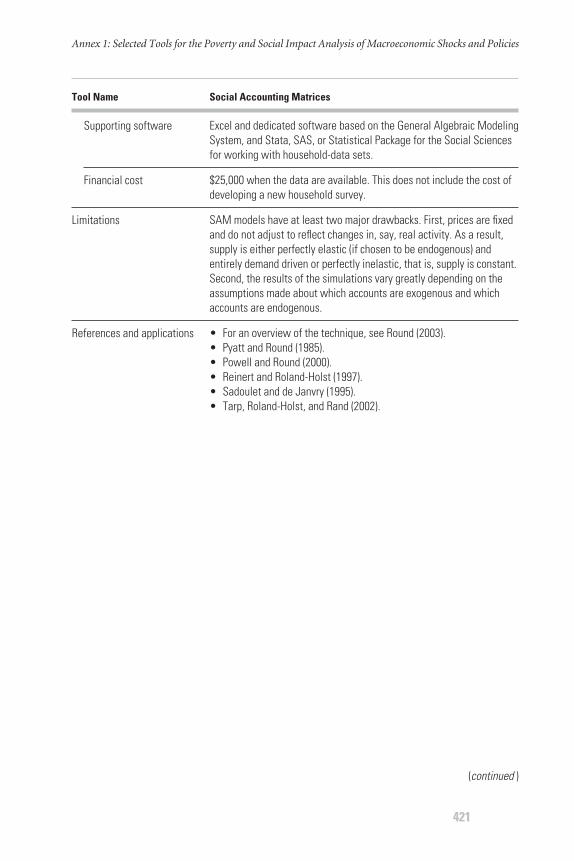
Annex 1: Selected Tools for the Poverty and Social Impact Analysis of Macroeconomic Shocks and Policies
421
Tool Name Social Accounting Matrices
Supporting software
Financial cost
Limitations
References and applications
Excel and dedicated software based on the General Algebraic ModelingSystem, and Stata, SAS, or Statistical Package for the Social Sciencesfor working with household-data sets.
$25,000 when the data are available. This does not include the cost ofdeveloping a new household survey.
SAM models have at least two major drawbacks. First, prices are fixedand do not adjust to reflect changes in, say, real activity. As a result,supply is either perfectly elastic (if chosen to be endogenous) andentirely demand driven or perfectly inelastic, that is, supply is constant.Second, the results of the simulations vary greatly depending on theassumptions made about which accounts are exogenous and whichaccounts are endogenous.
• For an overview of the technique, see Round (2003).• Pyatt and Round (1985).• Powell and Round (2000).• Reinert and Roland-Holst (1997).• Sadoulet and de Janvry (1995).• Tarp, Roland-Holst, and Rand (2002).
(continued )

What is it?
What can it be used for?
What does it tell you?
Complementary tools
Key elements
Requirements
Data/information
Time
Analyzing the Distributional Impact of Selected Reforms
422
CGE models are completely specified models of an economy or a region,including all production activities, factors, and institutions. The modelstherefore include the modeling of all markets (in which agent decisionsare price responsive, and markets reconcile supply and demand decisions)and macroeconomic components, such as investment and savings,balance of payments, and government budget.
CGE models can be used to analyze the poverty and social impacts of a wide range of policies, including exogenous shocks (exchange rate,international prices, and so on), changes in taxation, subsidies, andpublic expenditure (including changes in trade policies), and changes inthe domestic economic and social structure (including technologicalchanges, asset redistribution, and human capital formation).
CGE models are best chosen for policy analysis when the socioeconomicstructure, prices, and macroeconomic phenomena all prove important forthe analysis. They allow one to take into account all sectors of the econ-omy, as well as the macroeconomy, and, hence, permit the explicit exami-nation of both the direct and the indirect consequences of policies. This isparticularly important for those policy reforms that are likely to play a largerole in the economy and might have important impacts on other sectors oron the flow of foreign exchange or capital.
Other tools described here belong to this class of models, with an addi-tional model to take distribution into account: the 123PRSP, IMMPA,and the augmented CGE model with a representative householdapproach. See the respective tables in this annex.
A CGE can be described by specifying the agents and their behavior, the rules that bring the different markets in equilibrium, and the macro-economic characteristics. CGE models are based on SAMs (see the tableon social accounting matrices) and can be distinguished by the complex-ity and the level of disaggregation of productive activities, factors, andinstitutions, including households.
CGE models are data intensive. They are constructed from combinednational accounts and survey data. These are first compiled into aSAM, which is then used as the foundation of the CGE.
A few months to a year, depending on the existence of a SAM or ofanother CGE model built to address a different question. Even thesesimple CGEs can be complex and time consuming. An alternative is touse a previously constructed CGE. For example, Ianchovichina, Nicita,
TABLE A7.1. Selected Tools for the Poverty and Social Impact Analysis of Macroeconomic Shocks and Policies (Continued )
Tool Name Computable General Equilibrium Models
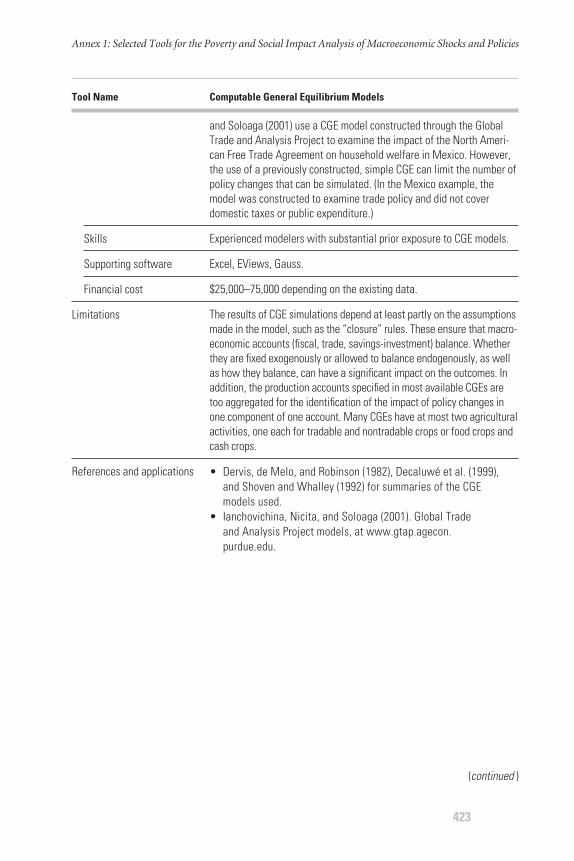
Skills
Supporting software
Financial cost
Limitations
References and applications
Annex 1: Selected Tools for the Poverty and Social Impact Analysis of Macroeconomic Shocks and Policies
423
Tool Name Computable General Equilibrium Models
and Soloaga (2001) use a CGE model constructed through the GlobalTrade and Analysis Project to examine the impact of the North Ameri-can Free Trade Agreement on household welfare in Mexico. However,the use of a previously constructed, simple CGE can limit the number ofpolicy changes that can be simulated. (In the Mexico example, themodel was constructed to examine trade policy and did not coverdomestic taxes or public expenditure.)
Experienced modelers with substantial prior exposure to CGE models.
Excel, EViews, Gauss.
$25,000–75,000 depending on the existing data.
The results of CGE simulations depend at least partly on the assumptionsmade in the model, such as the “closure” rules. These ensure that macro-economic accounts (fiscal, trade, savings-investment) balance. Whetherthey are fixed exogenously or allowed to balance endogenously, as wellas how they balance, can have a significant impact on the outcomes. Inaddition, the production accounts specified in most available CGEs aretoo aggregated for the identification of the impact of policy changes inone component of one account. Many CGEs have at most two agriculturalactivities, one each for tradable and nontradable crops or food crops andcash crops.
• Dervis, de Melo, and Robinson (1982), Decaluwé et al. (1999), and Shoven and Whalley (1992) for summaries of the CGE models used.
• Ianchovichina, Nicita, and Soloaga (2001). Global Trade and Analysis Project models, at www.gtap.agecon.purdue.edu.
(continued )

Analyzing the Distributional Impact of Selected Reforms
424
TABLE A7.1. Selected Tools for the Poverty and Social Impact Analysis of Macroeconomic Shocks and Policies (Continued )
Tool Name PovStat
What is it?
What can it be used for?
What does it tell you?
Complementary tools
Key elements
Requirements
Data/information
An Excel-based software program that simulates the changes inpoverty and inequality resulting over time from changes in growth inoutput and employment.
PovStat may be used to simulate the poverty and inequality impact of policies affecting sector-level output and employmentgrowth rates.
PovStat simulates poverty and inequality measures under alter-native growth scenarios. Forecasts of varying levels of complexitymay be computed, depending on the availability of reliable data and the extent to which factors influencing poverty levels are incorporated. The simulations vary according to optional projection parameters.
Other software programs that provide poverty and inequality fore-casts include SimSIP Poverty (see this annex on SimSIP) and DAD (a software for distributive analysis).
On the basis of household-level data, the software translates differential output and employment growth across sectors into differential growth in the per capita income or consumption of households across those sectors. The tool simulates the impact on poverty of policies affecting output. It does this by using the fact that poverty changes can be decomposed into two parts: a component related to the uniform growth of income and a component linked to changes in relative income. The simulations are made under the assumption that the policy analyzed will be distribution neutral or, conversely, that there is a specific, quantifiable form for the distributional change. Changes in employment distribution are accommodated by reweighing the sample households.
This program requires unit record household-survey data. Also, apoverty line, survey year, and forecast horizon are parameters thatmust be provided by the user. Macroeconomic variables at the nation-ally aggregated or sectorally disaggregated level and growth rates ofincome, employment, and population are also required. In addition, theuser can input changes in the CPI and GDP deflator, changes in the rel-ative prices of food and the shares of food in CPI, and changes in thepoverty-line-consumption bundle. This allows one to generate differ-ent types of forecasts and optional projection parameters such as

Annex 1: Selected Tools for the Poverty and Social Impact Analysis of Macroeconomic Shocks and Policies
425
Tool Name PovStat
Time
Skills
Supporting software
Financial cost
Limitations
References and applications
employment shifts across sectors. The software can be adapted forgrouped data.
One or two days to format the household-survey data, collate and checkexogenous economic variables, and enter everything into PovStat.
Familiarity with Excel and appropriate household-data-handling soft-ware (such as Stata). Also, familiarity with POVCAL if synthetic datafrom a grouped distribution are to be used.
Excel.
–
PovStat does not capture second-round effects. These may be capturedby CGE models.
• For an overview of the technique, see Datt et al. (2003).• Datt and Walker (2002).• Software available at www.worldbank.org/psia, “Tools and Methods.”
(continued )
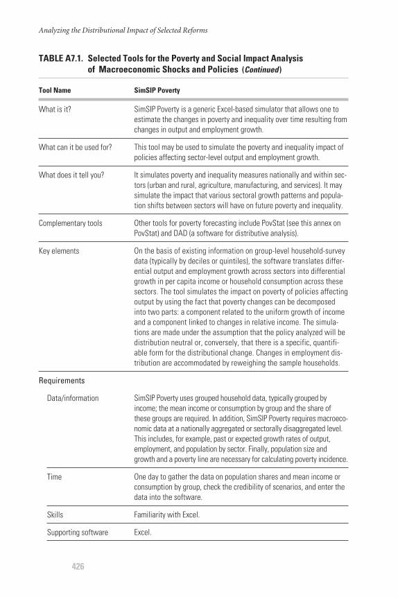
Analyzing the Distributional Impact of Selected Reforms
426
TABLE A7.1. Selected Tools for the Poverty and Social Impact Analysis of Macroeconomic Shocks and Policies (Continued )
Tool Name SimSIP Poverty
What is it?
What can it be used for?
What does it tell you?
Complementary tools
Key elements
Requirements
Data/information
Time
Skills
Supporting software
SimSIP Poverty is a generic Excel-based simulator that allows one toestimate the changes in poverty and inequality over time resulting fromchanges in output and employment growth.
This tool may be used to simulate the poverty and inequality impact ofpolicies affecting sector-level output and employment growth.
It simulates poverty and inequality measures nationally and within sec-tors (urban and rural, agriculture, manufacturing, and services). It maysimulate the impact that various sectoral growth patterns and popula-tion shifts between sectors will have on future poverty and inequality.
Other tools for poverty forecasting include PovStat (see this annex onPovStat) and DAD (a software for distributive analysis).
On the basis of existing information on group-level household-surveydata (typically by deciles or quintiles), the software translates differ-ential output and employment growth across sectors into differentialgrowth in per capita income or household consumption across thesesectors. The tool simulates the impact on poverty of policies affectingoutput by using the fact that poverty changes can be decomposedinto two parts: a component related to the uniform growth of incomeand a component linked to changes in relative income. The simula-tions are made under the assumption that the policy analyzed will bedistribution neutral or, conversely, that there is a specific, quantifi-able form for the distributional change. Changes in employment dis-tribution are accommodated by reweighing the sample households.
SimSIP Poverty uses grouped household data, typically grouped byincome; the mean income or consumption by group and the share ofthese groups are required. In addition, SimSIP Poverty requires macroeco-nomic data at a nationally aggregated or sectorally disaggregated level.This includes, for example, past or expected growth rates of output,employment, and population by sector. Finally, population size andgrowth and a poverty line are necessary for calculating poverty incidence.
One day to gather the data on population shares and mean income orconsumption by group, check the credibility of scenarios, and enter thedata into the software.
Familiarity with Excel.
Excel.
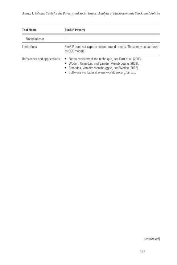
Annex 1: Selected Tools for the Poverty and Social Impact Analysis of Macroeconomic Shocks and Policies
427
Tool Name SimSIP Poverty
Financial cost
Limitations
References and applications
–
SimSIP does not capture second-round effects. These may be capturedby CGE models.
• For an overview of the technique, see Datt et al. (2003).• Wodon, Ramadas, and Van der Mensbrugghe (2003).• Ramadas, Van der Mensbrugghe, and Wodon (2002).• Software available at www.worldbank.org/simsip.
(continued )
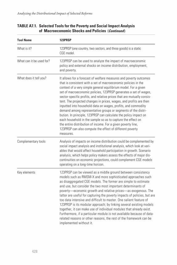
Analyzing the Distributional Impact of Selected Reforms
428
TABLE A7.1. Selected Tools for the Poverty and Social Impact Analysis of Macroeconomic Shocks and Policies (Continued )
Tool Name 123PRSP
What is it?
What can it be used for?
What does it tell you?
Complementary tools
Key elements
123PRSP (one country, two sectors, and three goods) is a static CGE model.
123PRSP can be used to analyze the impact of macroeconomic policy and external shocks on income distribution, employment, and poverty.
It allows for a forecast of welfare measures and poverty outcomesthat is consistent with a set of macroeconomic policies in the context of a very simple general equilibrium model. For a given set of macroeconomic policies, 123PRSP generates a set of wages,sector-specific profits, and relative prices that are mutually consis-tent. The projected changes in prices, wages, and profits are theninputted into household data on wages, profits, and commoditydemand among representative groups or segments of the distri-bution. In principle, 123PRSP can calculate the policy impact on each household in the sample so as to capture the effect on the entire distribution of income. For a given poverty line, 123PRSP can also compute the effect of different poverty measures.
Analysis of impacts on income distribution could be complemented bysocial impact analysis and institutional analysis, which look at vari-ables that would affect household participation in growth. Scenarioanalysis, which helps policy makers assess the effects of major dis-continuities on economic projections, could complement CGE modelsoperating on a long-time horizon.
123PRSP can be viewed as a middle ground between consistencymodels such as RMSM-X and more sophisticated approaches suchas disaggregated CGE models. The former are simple to estimateand use, but consider the two most important determinants ofpoverty—economic growth and relative prices—as exogenous. Thelatter are useful for capturing the poverty impacts of policies, but aretoo data intensive and difficult to master. One salient feature of123PRSP is its modular approach; by linking several existing modelstogether, it can make use of individual modules that already exist.Furthermore, if a particular module is not available because of data-related reasons or other reasons, the rest of the framework can beimplemented without it.
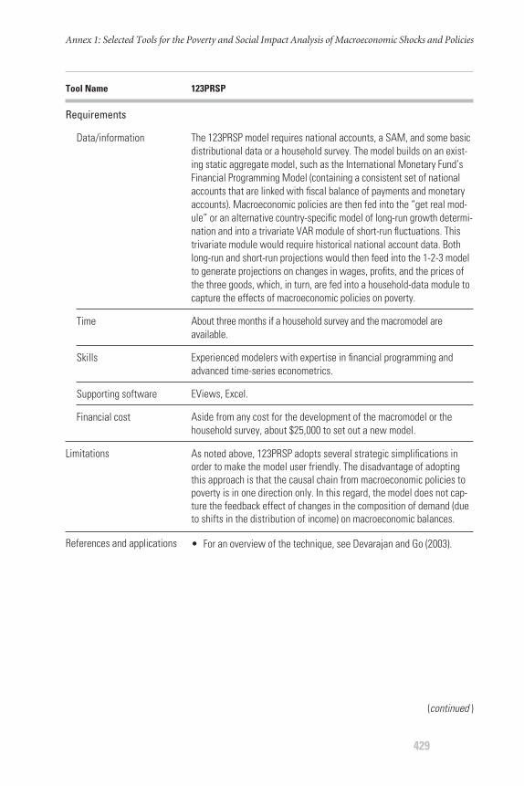
Annex 1: Selected Tools for the Poverty and Social Impact Analysis of Macroeconomic Shocks and Policies
429
Tool Name 123PRSP
Requirements
Data/information
Time
Skills
Supporting software
Financial cost
Limitations
References and applications
The 123PRSP model requires national accounts, a SAM, and some basicdistributional data or a household survey. The model builds on an exist-ing static aggregate model, such as the International Monetary Fund’sFinancial Programming Model (containing a consistent set of nationalaccounts that are linked with fiscal balance of payments and monetaryaccounts). Macroeconomic policies are then fed into the “get real mod-ule” or an alternative country-specific model of long-run growth determi-nation and into a trivariate VAR module of short-run fluctuations. Thistrivariate module would require historical national account data. Bothlong-run and short-run projections would then feed into the 1-2-3 modelto generate projections on changes in wages, profits, and the prices ofthe three goods, which, in turn, are fed into a household-data module tocapture the effects of macroeconomic policies on poverty.
About three months if a household survey and the macromodel are available.
Experienced modelers with expertise in financial programming andadvanced time-series econometrics.
EViews, Excel.
Aside from any cost for the development of the macromodel or thehousehold survey, about $25,000 to set out a new model.
As noted above, 123PRSP adopts several strategic simplifications inorder to make the model user friendly. The disadvantage of adoptingthis approach is that the causal chain from macroeconomic policies topoverty is in one direction only. In this regard, the model does not cap-ture the feedback effect of changes in the composition of demand (dueto shifts in the distribution of income) on macroeconomic balances.
• For an overview of the technique, see Devarajan and Go (2003).
(continued )
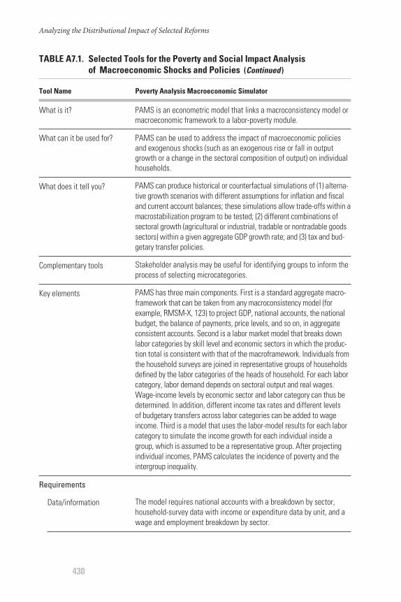
Analyzing the Distributional Impact of Selected Reforms
430
TABLE A7.1. Selected Tools for the Poverty and Social Impact Analysis of Macroeconomic Shocks and Policies (Continued )
Tool Name Poverty Analysis Macroeconomic Simulator
What is it?
What can it be used for?
What does it tell you?
Complementary tools
Key elements
Requirements
Data/information
PAMS is an econometric model that links a macroconsistency model ormacroeconomic framework to a labor-poverty module.
PAMS can be used to address the impact of macroeconomic policiesand exogenous shocks (such as an exogenous rise or fall in outputgrowth or a change in the sectoral composition of output) on individualhouseholds.
PAMS can produce historical or counterfactual simulations of (1) alterna-tive growth scenarios with different assumptions for inflation and fiscaland current account balances; these simulations allow trade-offs within amacrostabilization program to be tested; (2) different combinations ofsectoral growth (agricultural or industrial, tradable or nontradable goodssectors) within a given aggregate GDP growth rate; and (3) tax and bud-getary transfer policies.
Stakeholder analysis may be useful for identifying groups to inform theprocess of selecting microcategories.
PAMS has three main components. First is a standard aggregate macro-framework that can be taken from any macroconsistency model (forexample, RMSM-X, 123) to project GDP, national accounts, the nationalbudget, the balance of payments, price levels, and so on, in aggregateconsistent accounts. Second is a labor market model that breaks downlabor categories by skill level and economic sectors in which the produc-tion total is consistent with that of the macroframework. Individuals fromthe household surveys are joined in representative groups of householdsdefined by the labor categories of the heads of household. For each laborcategory, labor demand depends on sectoral output and real wages.Wage-income levels by economic sector and labor category can thus bedetermined. In addition, different income tax rates and different levels of budgetary transfers across labor categories can be added to wageincome. Third is a model that uses the labor-model results for each laborcategory to simulate the income growth for each individual inside agroup, which is assumed to be a representative group. After projectingindividual incomes, PAMS calculates the incidence of poverty and theintergroup inequality.
The model requires national accounts with a breakdown by sector,household-survey data with income or expenditure data by unit, and awage and employment breakdown by sector.
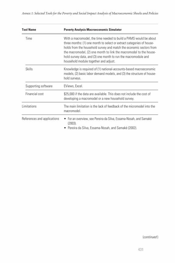
Annex 1: Selected Tools for the Poverty and Social Impact Analysis of Macroeconomic Shocks and Policies
431
Time
Skills
Supporting software
Financial cost
Limitations
References and applications
With a macromodel, the time needed to build a PAMS would be aboutthree months: (1) one month to select or extract categories of house-holds from the household survey and match the economic sectors fromthe macromodel, (2) one month to link the macromodel to the house-hold-survey data, and (3) one month to run the macromodule andhousehold module together and adjust.
Knowledge is required of (1) national-accounts-based macroeconomicmodels, (2) basic labor demand models, and (3) the structure of house-hold surveys.
EViews, Excel.
$25,000 if the data are available. This does not include the cost ofdeveloping a macromodel or a new household survey.
The main limitation is the lack of feedback of the micromodel into themacromodel.
• For an overview, see Pereira da Silva, Essama-Nssah, and Samaké(2003).
• Pereira da Silva, Essama-Nssah, and Samaké (2002).
(continued )
Tool Name Poverty Analysis Macroeconomic Simulator
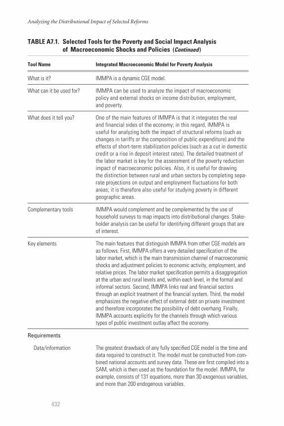
Analyzing the Distributional Impact of Selected Reforms
432
TABLE A7.1. Selected Tools for the Poverty and Social Impact Analysis of Macroeconomic Shocks and Policies (Continued )
Tool Name Integrated Macroeconomic Model for Poverty Analysis
What is it?
What can it be used for?
What does it tell you?
Complementary tools
Key elements
Requirements
Data/information
IMMPA is a dynamic CGE model.
IMMPA can be used to analyze the impact of macroeconomic policy and external shocks on income distribution, employment, and poverty.
One of the main features of IMMPA is that it integrates the real and financial sides of the economy; in this regard, IMMPA is useful for analyzing both the impact of structural reforms (such aschanges in tariffs or the composition of public expenditure) and theeffects of short-term stabilization policies (such as a cut in domesticcredit or a rise in deposit interest rates). The detailed treatment ofthe labor market is key for the assessment of the poverty reductionimpact of macroeconomic policies. Also, it is useful for drawing the distinction between rural and urban sectors by completing sepa-rate projections on output and employment fluctuations for bothareas; it is therefore also useful for studying poverty in differentgeographic areas.
IMMPA would complement and be complemented by the use ofhousehold surveys to map impacts into distributional changes. Stake-holder analysis can be useful for identifying different groups that areof interest.
The main features that distinguish IMMPA from other CGE models areas follows. First, IMMPA offers a very detailed specification of thelabor market, which is the main transmission channel of macroeconomicshocks and adjustment policies to economic activity, employment, andrelative prices. The labor market specification permits a disaggregationat the urban and rural levels and, within each level, in the formal andinformal sectors. Second, IMMPA links real and financial sectorsthrough an explicit treatment of the financial system. Third, the modelemphasizes the negative effect of external debt on private investmentand therefore incorporates the possibility of debt overhang. Finally,IMMPA accounts explicitly for the channels through which varioustypes of public investment outlay affect the economy.
The greatest drawback of any fully specified CGE model is the time anddata required to construct it. The model must be constructed from com-bined national accounts and survey data. These are first compiled into aSAM, which is then used as the foundation for the model. IMMPA, forexample, consists of 131 equations, more than 30 exogenous variables,and more than 200 endogenous variables.
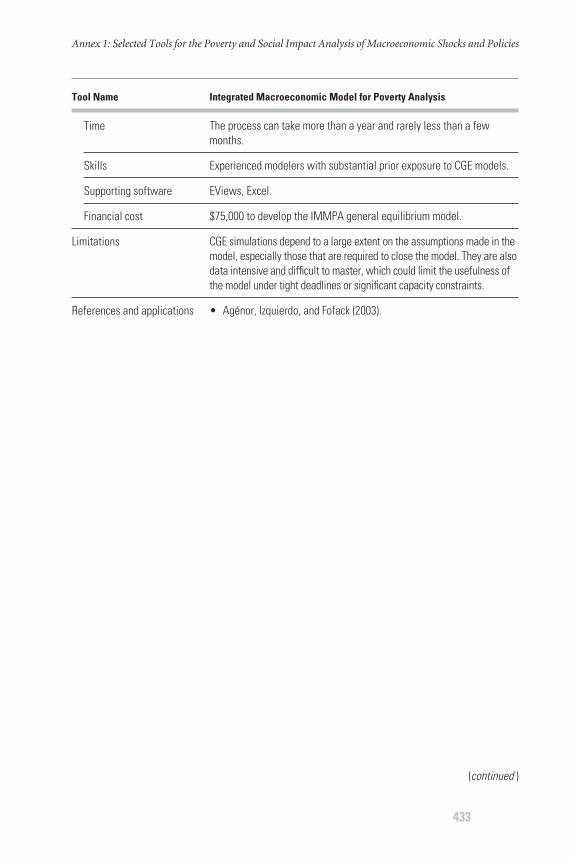
Annex 1: Selected Tools for the Poverty and Social Impact Analysis of Macroeconomic Shocks and Policies
433
Time
Skills
Supporting software
Financial cost
Limitations
References and applications
The process can take more than a year and rarely less than a fewmonths.
Experienced modelers with substantial prior exposure to CGE models.
EViews, Excel.
$75,000 to develop the IMMPA general equilibrium model.
CGE simulations depend to a large extent on the assumptions made in themodel, especially those that are required to close the model. They are alsodata intensive and difficult to master, which could limit the usefulness ofthe model under tight deadlines or significant capacity constraints.
• Agénor, Izquierdo, and Fofack (2003).
Tool Name Integrated Macroeconomic Model for Poverty Analysis
(continued )

This technique is based on a CGE model with representative house-holds that are linked to a household module.
RH models can be used to analyze the impact of macroeconomic policyand external shocks on income distribution, employment, and poverty.
RH models allow for a forecast of welfare measures and poverty out-comes consistent with a set of macroeconomic policies in the contextof a general equilibrium model.
–
The key features of the RH approach are, first, a CGE model that incorpo-rates markets for factors and commodities and their links to the rest of theeconomy and that generates equilibrium values for employment, wages,and commodity prices, as well as “extended” functional distributions (thatis, labor differentiated by skill, education, gender, region, and sector ofemployment) and, second, a mapping from the extended functional distribu-tion into the “size” distribution (the distribution of income across differenthouseholds). In this approach, the representative households that appear inthe CGE (corresponding to aggregates or averages of groups of households)play a crucial role: the “size” distribution is generated by feeding data onthe simulated outcomes for the representative households into a separatemodule that contains additional information about each household.
RH models require a SAM and distributional data describing the repre-sentative household groups or, more specifically, a household survey.
Only a few days to generate a base solution if data and skills are avail-able. Between six months and a year to collect data and work with thesimulations.
Experienced modelers with substantial prior exposure to CGE models.
Excel, EViews, Gauss.
$25,000–75,000 depending on the data that exist.
Analyzing the Distributional Impact of Selected Reforms
434
TABLE A7.1. Selected Tools for the Poverty and Social Impact Analysis of Macroeconomic Shocks and Policies (Continued )
Tool Name Augmented CGE Model with the Representative Household Approach
What is it?
What can it be used for?
What does it tell you?
Complementary tools
Key elements
Requirements
Data/information
Time
Skills
Supporting software
Financial cost
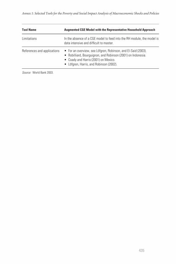
Limitations
References and applications
Source: World Bank 2003.
Annex 1: Selected Tools for the Poverty and Social Impact Analysis of Macroeconomic Shocks and Policies
435
In the absence of a CGE model to feed into the RH module, the model isdata intensive and difficult to master.
• For an overview, see Löfgren, Robinson, and El-Said (2003).• Robilliard, Bourguignon, and Robinson (2001) on Indonesia.• Coady and Harris (2001) on Mexico.• Löfgren, Harris, and Robinson (2002).
Tool Name Augmented CGE Model with the Representative Household Approach
