machine learning: linear regression and neural networks

DM534

INTRODUCTION TO COMPUTER SCIENCE

Machine Learning:Linear Regression and Neural Networks

Marco Chiarandini

Department of Mathematics & Computer ScienceUniversity of Southern Denmark

Machine LearningLinear RegressionArti�cial Neural NetworksAbout Me (https://imada.sdu.dk/~marco)

• Marco Chiarandini, Asc. Prof. in CS at IMADA• Master in Electronic Engineering, University of Udine, Italy.

• Ph.D. in Computer Science at the Darmstadt University ofTechnology, Germany.

• Post-Doc researcher at IMADA

• Visiting Researcher, Institute of Interdisciplinary Research andDevelopment in Artifcial Intelligence, Université Libre de Bruxelles.

• Research Interests

• Optimization (Operations Research) | Scheduling, Timetabling, Routing

• Arti�cial Intelligence | Heuristics, Metaheuristics, Machine Learning

• Current Teaching in CS

• Linear Algebra and Applications (Bachelor)

• Linear and Integer Programming (Master)

• Mathematical Optimization at Work (Master)

• Constraint Programming (Master)

• Arti�cial Intelligence (Master)

2

https://imada.sdu.dk/~marco

Machine LearningLinear RegressionArti�cial Neural NetworksOutline

1. Machine Learning

2. Linear RegressionExtensions

3. Arti�cial Neural NetworksSingle-layer NetworksMulti-layer perceptrons

3


1. Machine Learning



4

Machine LearningLinear RegressionArti�cial Neural NetworksMachine Learning

An agent is learning if it improves its performance on future tasks after making observations aboutthe world.

Why learning instead of directly programming?

Three main situations:

• the designer cannot anticipate all possible solutions

• the designer cannot anticipate all changes over time

• the designer has no idea how to program a solution(see, for example, face recognition)

5

Machine LearningLinear RegressionArti�cial Neural NetworksForms of Machine Learning

• Supervised learning (this week)the agent is provided with a series of examples with correct responses and then it generalizes from those examples to

develop an algorithm that applies to new cases.

Eg: learning to recognize a person's handwriting or voice, to distinguish between junk and welcome email, or to identify a

disease from a set of symptoms.

• Unsupervised learning (with Melih Kandemir)Correct responses are not provided, but instead the agent tries to identify similarities between the inputs so that inputs

that have something in common are categorised together.

Eg. Clustering

• Reinforcement learning:the agent is given a general rule to judge for itself when it has succeeded or failed at a task during trial and error. The

agent acts autonomously and it learns to improve its behavior over time.

Eg: learning how to play a game like backgammon (success or failure is easy to de�ne)

6

Machine LearningLinear RegressionArti�cial Neural NetworksSupervised Learning

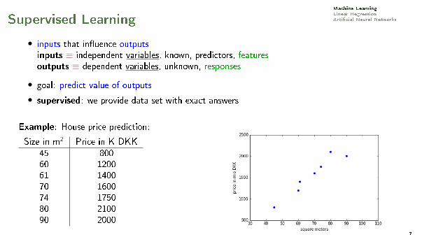
• inputs that in�uence outputsinputs ≡ independent variables, known, predictors, featuresoutputs ≡ dependent variables, unknown, responses

• goal: predict value of outputs

• supervised: we provide data set with exact answers

Example: House price prediction:

Size in m2 Price in K DKK45 80060 120061 140070 160074 175080 210090 2000

7

Machine LearningLinear RegressionArti�cial Neural NetworksSupervised Learning Problem

Given: m points (pairs of numbers) {(x1, y1), (x2, y2), . . . , (xm, ym)}

Task: determine a model, aka a function g(x) of a simple form, such that

g(x1) ≈ y1,g(x2) ≈ y2,

...g(xm) ≈ ym.

• We denote by y = g(x) the response value predicted by g on x .

• The type of function (linear, polynomial, exponential, logistic, blackbox) may be suggested bythe nature of the problem (the underlying physical law, the type of response).It is a form of prior knowledge.

In other words, we are �tting a function to the data

8

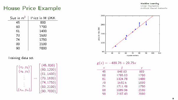
Machine LearningLinear RegressionArti�cial Neural NetworksHouse Price Example

Size in m2 Price in M DKK

45 80060 120061 140070 160074 175080 210090 2000

Training data set

(x1, y1)(x2, y2)

...

...(xm, ym)

(45, 800)(60, 1200)(61, 1400)(70, 1600)(74, 1750)(80, 2100)(90, 2000)

g(x) = −489.76+ 29.75x

x y y45 848.83 800

60 1295.03 1200

61 1324.78 1400

70 1592.5 1600

74 1711.48 1750

80 1889.96 2100

90 2187.43 2000

9

Machine LearningLinear RegressionArti�cial Neural NetworksTypes of Supervised Learning

Regression problem:variable to predict is continuous/quantitative

Classi�cation problem:variable to predict is discrete/qualitative

10

Machine LearningLinear RegressionArti�cial Neural NetworksExample: k-Nearest Neighbors

Regression task

Given: (x1, y1), . . . , (xm, ym)Task: predict the response value y for a new input x

Idea: Let y(x) be the average of the k closest points:

1. Sort the data points (x1, y1), . . . , (xm, ym) in increasing order of distance from x in the inputspace, ie, d(xi , x) = |xi − x |.

2. Set the k closest points in Nk(x).

3. Return the average of the y values of the k data points in Nk(x).

In mathematical notation:

y(x) =1

k

∑xi∈Nk (x)

yi = g(x)

11

Machine LearningLinear RegressionArti�cial Neural NetworksExample: k-Nearest Neighbors

Classi�cation task

Given: (x1, y1), . . . , (xm, ym)Task: predict the class y for a new input x .

Idea: let the k closest points vote and majority decide

1. Sort the data points (x1, y1), . . . , (xm, ym) in increasing order of distance from ~x in the inputspace, ie, d(~xi , ~x) = |xi − x |.

2. Set the k closest points in Nk(x).

3. Return the class that is most represented in the k data points of Nk(x).

This can also be expressed mathematically y = G (x) = . . .let's omit this here for the sake of simplicity

12


1. Machine Learning



13

Machine LearningLinear RegressionArti�cial Neural NetworksLinear Regression with One Variable

• Let the set of models we can use (hypothesis set) H be made by linear functions y = ax + b.We search in H the line that �ts best the data:

1. We evaluate each line by the distance of the points (x1, y1), . . . , (xm, ym) from the line inthe vertical direction (the y -direction):Each point (xi , yi ), i = 1..m would have predicted yi -value y = axi + b in the �tted line.Hence, the distance for (xi , yi ) is |yi − axi − b|.

2. We de�ne as loss (or error, or cost) function the sum of the squares of the distances fromthe given points (x1, y1), . . . , (xm, ym):

L(a, b) =m∑i=1

(yi − axi − b)2 sum of squared errors

L depends on a and b, while the values xi and yi are given by the data available.

3. We look for the coe�cients a and b that give the line of minimal loss (here, sum ofsquared errors, hence also known as method of least squares).

14


Training data set

(x1, y1)(x2, y2)

...

...(xm, ym)

=⇒

(45, 800)(60, 1200)(61, 1400)(70, 1600)(74, 1750)(80, 2100)(90, 2000)

g(x) = 29.75x − 489.76

x y y45 848.83 800

60 1295.03 1200

61 1324.78 1400

70 1592.5 1600

74 1711.48 1750

80 1889.96 2100

90 2187.43 2000

L =∑m

i=1(yi − yi )2 =

= (800− 848.83)2

+(1200− 1295.03)2

+(1400− 1324.78)2

+(1600− 1592.5)2

+(1750− 1711.48)2

+(2100− 1889.96)2

+(2000− 2187.43)2 = 97858.8615


For

f (x) = b + ax

L(a, b) =∑m

i=1(yi − yi )2

= (800− b − 45 · a)2+(1200− b − 60 · a)2+(1400− b − 61 · a)2+(1600− b − 70 · a)2+(1750− b − 74 · a)2+(2100− b − 80 · a)2+(2000− b − 90 · a)2

Plot of L(a, b) as a function of a and b:

16

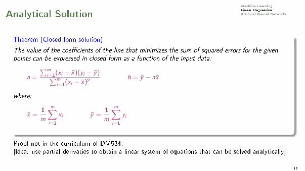
Machine LearningLinear RegressionArti�cial Neural NetworksAnalytical Solution

Theorem (Closed form solution)

The value of the coe�cients of the line that minimizes the sum of squared errors for the given

points can be expressed in closed form as a function of the input data:

a =

∑mi=1(xi − x)(yi − y)∑m

i=1(xi − x)2b = y − ax

where:

x =1

m

m∑i=1

xi y =1

m

m∑i=1

yi

Proof not in the curriculum of DM534:[Idea: use partial derivaties to obtain a linear system of equations that can be solved analytically]

17

Machine LearningLinear RegressionArti�cial Neural NetworksMachine Learning: The General Framework

Learning = Representation + Evaluation + Optimization

• Representation: formal language that the computer can handle. Corresponds to choosing theset of functions that can be learned, ie. the hypothesis set of the learner. How to represent theinput, that is, which input variables to use.

• Evaluation: de�nition of a loss function

• Optimization: a method to search among the learners in the language for the one minimizingthe loss.

18

Machine LearningLinear RegressionArti�cial Neural NetworksLearning model

19


1. Machine Learning



20

Machine LearningLinear RegressionArti�cial Neural NetworksLinear Regression with Multiple Variables

There can be several input variables (aka features). In practice, they improve prediction.

Size in m2 # of rooms · · · Price in M DKK45 2 · · · 80060 3 · · · 120061 2 · · · 140070 3 · · · 160074 3 · · · 175080 3 · · · 210090 4 · · · 2000...

......

In vector notation:

(~x1, y1)(~x2, y2)

...(~xm, ym)

~xi =[xi1 xi2 . . . xip

]i = 1, 2, . . . ,m

21

Machine LearningLinear RegressionArti�cial Neural Networksk-Nearest Neighbors Revisited

Case with multiple input variables

Regression task

Given: (~x1, y1), . . . , (~xm, ym)Task: predict the response value y for a new input ~x

Idea: Let y(~x) be the average of the k closest points:

1. Sort the data points (~x1, y1), . . . , (~xm, ym) in increasing order of distance from x in the input

space, ie, d(~xi , ~x) =√∑

j(xij − xj)2.

2. Set the k closest points in Nk(~x).

3. Return the average of the y values of the k data points in Nk(~x).

In mathematical notation:

y(~x) =1

k

∑~xi∈Nk (~x)

yi = g(~x)

It requires the rede�nition of the distance metric, eg, Euclidean distance22

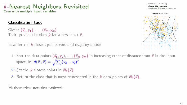
Machine LearningLinear RegressionArti�cial Neural Networksk-Nearest Neighbors Revisited

Case with multiple input variables

Classi�cation task

Given: (~x1, y1), . . . , (~xm, ym)Task: predict the class y for a new input ~x .

Idea: let the k closest points vote and majority decide

1. Sort the data points (~x1, y1), . . . , (~xm, ym) in increasing order of distance from ~x in the input

space, ie, d(~xi , ~x) =√∑

j(xij − xj)2.

2. Set the k closest points in Nk(~x).

3. Return the class that is most represented in the k data points of Nk(~x).

Mathematical notation omitted.

23

Machine LearningLinear RegressionArti�cial Neural NetworksLinear Regression Revisited

Representation of hypothesis space if only one variable (feature):

h(x) = θ0 + θ1x linear function

if there is another input variable (feature):

h(x) = θ0 + θ1x1 + θ2x2 = h(~θ, ~x)

for conciseness, de�ning x0 = 1.

h(~θ, ~x) = ~θ · ~x =2∑

j=0

θjxj h(~θ, ~xi ) = ~θ · ~xi =

p∑j=0

θjxij

Notation:

• p num. of features, ~θ vector of p + 1 coe�cients, θ0 is the bias

• xij is the value of feature j in sample i , for i = 1..m, j = 0..p

• yi is the value of the response in sample i24

Machine LearningLinear RegressionArti�cial Neural NetworksLinear Regression Revisited

Evaluation

loss function for penalizing errors in prediction.Most common is squared error loss:

L(~θ) =m∑i=1

(yi − h(~θ, ~xi )

)2=

m∑i=1

yi −p∑

j=0

θjxij

2

loss function

Optimization

min~θ

L(~θ)

Although not shown here, the optimization problem can be solved analytically and the solutioncan be expressed in closed form.

25

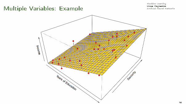
Machine LearningLinear RegressionArti�cial Neural NetworksMultiple Variables: Example

26

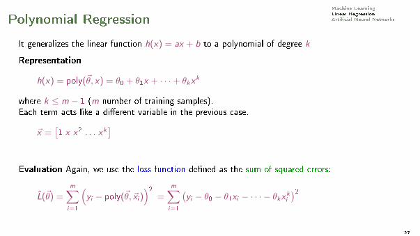
Machine LearningLinear RegressionArti�cial Neural NetworksPolynomial Regression

It generalizes the linear function h(x) = ax + b to a polynomial of degree k

Representation

h(x) = poly(~θ, x) = θ0 + θ1x + · · ·+ θkxk

where k ≤ m − 1 (m number of training samples).Each term acts like a di�erent variable in the previous case.

~x =[1 x x2 . . . xk

]

Evaluation Again, we use the loss function de�ned as the sum of squared errors:

L(~θ) =m∑i=1

(yi − poly(~θ, ~xi )

)2=

m∑i=1

(yi − θ0 − θ1xi − · · · − θkxki

)227

Machine LearningLinear RegressionArti�cial Neural NetworksPolynomial Regression

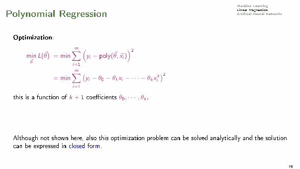
Optimization:

min~θ

L(~θ) = minm∑i=1

(yi − poly(~θ, ~xi )

)2= min

m∑i=1

(yi − θ0 − θ1xi − · · · − θkxki

)2this is a function of k + 1 coe�cients θ0, · · · , θk .

Although not shown here, also this optimization problem can be solved analytically and the solutioncan be expressed in closed form.

28

Machine LearningLinear RegressionArti�cial Neural NetworksPolynomial Regression: Example

29

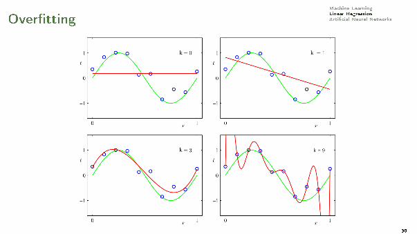
Machine LearningLinear RegressionArti�cial Neural NetworksOver�tting

30

Machine LearningLinear RegressionArti�cial Neural NetworksTraining and Assessment

Avoid peeking: use di�erent data for di�erent tasks:

Training and Test data

• Coe�cients learned on Training data

• Coe�cients and models compared on Validation data

• Final assessment on Test data

Techniques:

• Holdout method

• If small data:k-fold cross validation

31

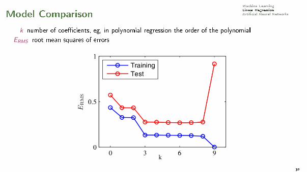
Machine LearningLinear RegressionArti�cial Neural NetworksModel Comparison

k number of coe�cients, eg, in polynomial regression the order of the polynomial

ERMS root mean squares of errors

32


1. Machine Learning



33

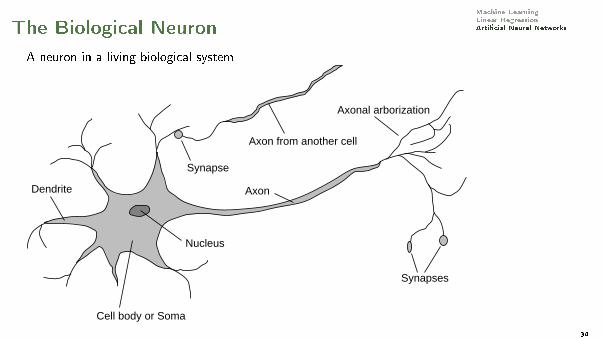
Machine LearningLinear RegressionArti�cial Neural NetworksThe Biological Neuron

A neuron in a living biological system

Axon

Cell body or Soma

Nucleus

Dendrite

Synapses

Axonal arborization

Axon from another cell

Synapse

Signals are noisy �spike trains� of electrical potential34

Machine LearningLinear RegressionArti�cial Neural NetworksMcCulloch�Pitts �unit� (1943)

Activities within a processing unit

35

Machine LearningLinear RegressionArti�cial Neural NetworksArti�cial Neural Networks

Basic idea:

• Arti�cial Neuron

• Each input is multiplied by a weighting factor.

• Output is 1 if sum of weighted inputs exceeds the threshold value;0 otherwise.

• Network is programmed by adjusting weights using feedback from examples.

�The neural network� does not exist. There are di�erent paradigms for neural networks, how theyare trained and where they are used.

36

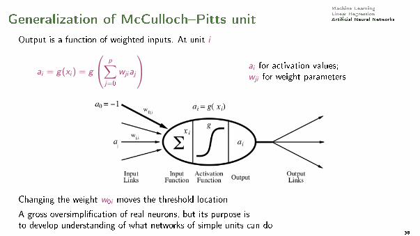
Machine LearningLinear RegressionArti�cial Neural NetworksGeneralization of McCulloch�Pitts unit

Let aj be the jth input to a node:Then, the output of the unit is 1 when:

−2a1 + 3a2 − 1a3 ≥ 1.5

or equivalently when:

−1.5− 2a1 + 3a2 − 1a3 ≥ 0

and, de�ning a0 = −1, when:

1.5a0 − 2a1 + 3a2 − 1a3 ≥ 0

In general, for a neuron i and weights wji on arcs ji , the neuron outputs 1 when:

p∑j=0

wjiaj ≥ 0,

and 0 otherwise. (We will assume the zeroth input a0 to always be −1.)37


Hence, we can draw the arti�cial neuron unit i :

w1i

w2i w0iw3i

a1

a2

a3

ai

also in the following way:

w0i

a0 = −1

w1ia1w2i

a2 w3i

a3

ai

where now the output ai is 1 when the linear combination of the inputs:

xi =

p∑j=0

wjiaj = ~wi · ~a ~a =[−1 a1 a2 · · · ap

]is > 0.

38


Output is a function of weighted inputs. At unit i

ai = g(xi ) = g

p∑j=0

wjiaj

ai for activation values;wji for weight parameters

Changing the weight w0i moves the threshold location

A gross oversimpli�cation of real neurons, but its purpose isto develop understanding of what networks of simple units can do

39

Machine LearningLinear RegressionArti�cial Neural NetworksActivation functions

Non linear activation functions

step function or threshold function(mostly used in theoretical studies)

perceptron

continuous activation function, e.g., sigmoidfunction 1/(1 + e−xi )sigmoid neuron

1/(1+ e−xi )

40

Machine LearningLinear RegressionArti�cial Neural NetworksActivation functions

41

Machine LearningLinear RegressionArti�cial Neural NetworksImplementing logical functions

AND

W0 = 1.5

W1 = 1

W2 = 1

OR

W2 = 1

W1 = 1

W0 = 0.5

NOT

W1 = –1

W0 = – 0.5

But not every Booelan function can be implemented by a perceptron. Exclusive-or circuit cannotbe processed (see next slide).

McCulloch and Pitts (1943) �rst mathematical model of neurons. Every Boolean function can beimplemented by combining this type of units.

Rosenblatt (1958) showed how to learn the parameters of a perceptron. Minsky and Papert (1969)lamented the lack of a mathematical rigor in learning in multilayer networks.

42

Machine LearningLinear RegressionArti�cial Neural NetworksExpressiveness of single perceptrons

Consider a perceptron with g step functionAt unit i the output is 1 when:

p∑j=0

wjixj > 0 or ~wi · ~x > 0

Hence, it represents a linear separator in input space:- line in 2 dimensions- plane in 3 dimensions- hyperplane in multidimensional space

43

These points are notlinearly separable

Machine LearningLinear RegressionArti�cial Neural NetworksNetwork structures

Structure (or architecture): de�nition of number of nodes, interconnections and activationfunctions g (but not weights).

• Feed-forward networks:no cycles in the connection graph

• single-layer perceptrons (no hidden layer)

• multi-layer perceptrons (one or more hidden layer)

Feed-forward networks implement functions, have no internal state

• Recurrent networks:connections between units form a directed cycle.� internal state of the networkexhibit dynamic temporal behavior (memory, apriori knowledge)

� Hop�eld networks for associative memory

44

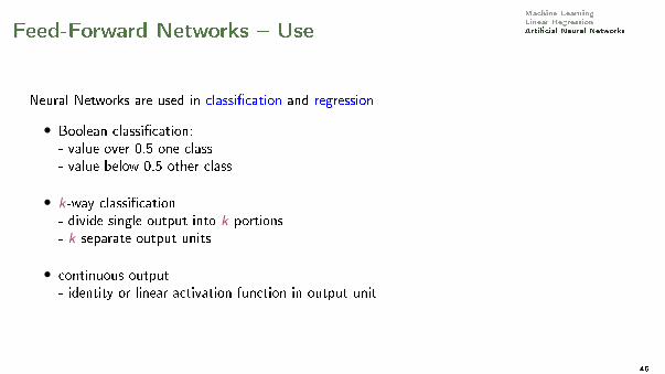
Machine LearningLinear RegressionArti�cial Neural NetworksFeed-Forward Networks � Use

Neural Networks are used in classi�cation and regression

• Boolean classi�cation:- value over 0.5 one class- value below 0.5 other class

• k-way classi�cation- divide single output into k portions- k separate output units

• continuous output- identity or linear activation function in output unit

45


1. Machine Learning



46

Machine LearningLinear RegressionArti�cial Neural NetworksSingle-layer NN

InputUnits Units

OutputWj,i

Output units all operate separately�no shared weightsAdjusting weights moves the location, orientation, and steepness of cli�

47


1. Machine Learning



48

Machine LearningLinear RegressionArti�cial Neural NetworksMultilayer perceptrons

Layers are usually fully connected;number of hidden units typically chosen by hand

Input units

Hidden units

Output units ai

Wj,i

aj

Wk,j

ak

(a for activation values; W for weight parameters)49

Machine LearningLinear RegressionArti�cial Neural NetworksMultilayer Feed-forward

W1,3

1,4W

2,3W

2,4W

W3,5

4,5W

1

2

3

4

5

Feed-forward network = a parametrized family of nonlinear functions:

a5 = g(w3,5 · a3 + w4,5 · a4)

= g(w3,5 · g(w1,3 · a1 + w2,3 · a2) + w4,5 · g(w1,4 · a1 + w2,4 · a2))

Adjusting weights changes the function: do learning this way!50

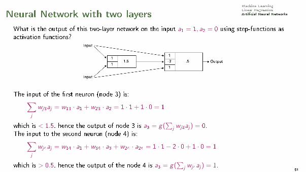
Machine LearningLinear RegressionArti�cial Neural NetworksNeural Network with two layers

What is the output of this two-layer network on the input a1 = 1, a2 = 0 using step-functions asactivation functions?

The input of the �rst neuron (node 3) is:∑j

wj3aj = w13 · a1 + w23 · a2 = 1 · 1 + 1 · 0 = 1

which is < 1.5, hence the output of node 3 is a3 = g(∑

j wj3aj) = 0.The input to the second neuron (node 4) is:∑

j

wj4aj = w14 · a1 + w34 · a3 + w24 · a24 = 1 · 1− 2 · 0 + 1 · 0 = 1

which is > 0.5, hence the output of the node 4 is a3 = g(∑

j wj4aj) = 1.51

Machine LearningLinear RegressionArti�cial Neural NetworksExpressiveness of MLPs

All continuous functions with 2 layers, all functions with 3 layers

-4 -2 0 2 4x1-4

-20

24

x2

00.20.40.60.8

1

hW(x1, x2)

-4 -2 0 2 4x1-4

-20

24

x2

00.20.40.60.8

1

hW(x1, x2)

Combine two opposite-facing threshold functions to make a ridgeCombine two perpendicular ridges to make a bumpAdd bumps of various sizes and locations to �t any surfaceProof requires exponentially many hidden units (Minsky & Papert, 1969)

52

Machine LearningLinear RegressionArti�cial Neural NetworksA Practical Example

Deep learning ≡convolutional neural networks ≡multilayer neural network with structureon the arcs

Example: one layer only for imagerecognition, another for action decision.

The image can be subdivided in regionsand each region linked only to a subset ofnodes of the �rst layer.

53

Machine LearningLinear RegressionArti�cial Neural NetworksNumerical Example

The Fisher's iris �ower data set: data to quantify the morphologic variation of Iris �owers of tworelated species.50 samples from each of two species of Iris (Iris setosa and Iris versicolor). Four features weremeasured from each sample: the length and the width of the petals and sepals, in centimeters.

Source: Medium

54

Machine LearningLinear RegressionArti�cial Neural NetworksNumerical Example

Binary Classi�cation

Preliminary observations show that measurments the petals can be enough for the task ofclassifying: iris setosa and iris versicolor.

4 5 6 7 8

1.0

1.5

2.0

2.5

3.0

3.5

4.0

4.5

Petal Dimensions in Iris Blossoms

Length

Wid

th

SS

SSS

S

S

S

SS S

S SS

S

S

S

SS

S

S

S S

S

S V

V

V

V

V V

V

V V

VV

V

V

VVV

VV

V

VVV

VV

V

SV

Setosa PetalsVersicolor Petals

iris.data:

Petal.Length Petal.Width Species id

4.9 3.1 setosa 0

5.5 2.6 versicolor 1



5.2 3.4 setosa 0


Two classes encoded as 0/1

55

Machine LearningLinear RegressionArti�cial Neural NetworksPerceptron Learning

In 2D, the decision surface of a linear combination of inputs gives: ~w · ~x = constant, a line!Training the perceptron ≡ searching the line that separates the points at best.

4 5 6 7 8

1.0

1.5

2.0

2.5

3.0

3.5

4.0

4.5


Length

Wid

th

SS

SSS

S

S

S

SS S

S SS

S

S

S

SS

S

S

S S

S

S V

V

V

V

V V

V

V V

VV

V

V

VVV

VV

V

VVV

VV

V

SV


grey lines: lines tried during the gradientdescent algorithmred line: the �nal line indicated by thegradient descent algorithm

57

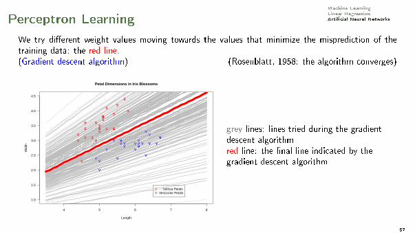
Machine LearningLinear RegressionArti�cial Neural NetworksPerceptron Learning

We try di�erent weight values moving towards the values that minimize the misprediction of thetraining data: the red line.(Gradient descent algorithm) (Rosenblatt, 1958: the algorithm converges)

4 5 6 7 8

1.0

1.5

2.0

2.5

3.0

3.5

4.0

4.5


Length

Wid

th

S

S

S

S

SS

S

SS

S

S

S

S

SS

S

SS

S

S

S

SS

SS

V V

V

V

V

V VV

V

V

V

V

V

V

VV

VV

VVV V

V

V

V

SV


S

S

S

S

SS

S

SS

S

S

S

S

SS

S

SS

S

S

S

SS

SS

V V

V

V

V

V VV

V

V

V

V

V

V

VV

VV

VVV V

V

V

V

grey lines: lines tried during the gradientdescent algorithmred line: the �nal line indicated by thegradient descent algorithm

57

Machine LearningLinear RegressionArti�cial Neural NetworksSummary

1. Machine Learning



59

machine learning: linear regression and neural networks

Documents