machine learning 1: linear regression - stanford universityermon/cs325/slides/ml_linear_reg.pdf ·...

Machine Learning 1: Linear Regression

Stefano Ermon

March 31, 2016

Stefano Ermon Machine Learning 1: Linear Regression March 31, 2016 1 / 25

Plan for today

Plan for today:

Supervised Machine Learning: linear regression


Renewable electricity generation in the U.S

Source: Renewable energy data book, NREL


Challenges for the grid

Wind and solar are intermittent

We will need traditional power plants when the wind stops

Many power plants (e.g., nuclear) cannot be easily turned on/off orquickly ramped up/down

With more accurate forecasts, wind and solar power become moreefficient alternatives

A few years ago, Xcel Energy (Colorado) ran ads opposing a proposalthat it use 10% of renewable sources

Thanks to wind forecasting (ML) algorithms developed at NCAR, theynow aim for 30 percent. Accurate forecasting saved the utility $6-$10million per year


Motivation

Solar and wind are intermittent

Can we accurately forecast how much energy will we consumetomorrow?

Difficult to estimate from “a priori” models

But, we have lots of data from which to build a model


Typical electricity consumption

0 5 10 15 201

1.5

2

2.5

3

Hour of Day

Hou

rly D

eman

d (G

W)

Feb 9Jul 13Oct 10

Data: PJM http://www.pjm.com


http://www.pjm.com

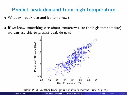
Predict peak demand from high temperature

What will peak demand be tomorrow?

If we know something else about tomorrow (like the high temperature),we can use this to predict peak demand

60 65 70 75 80 85 90 95

1.5

2

2.5

3

High Temperature (F)

Pea

k H

ourly

Dem

and

(GW

)

Data: PJM, Weather Underground (summer months, June-August)Stefano Ermon Machine Learning 1: Linear Regression March 31, 2016 7 / 25

A simple model

A linear model that predicts demand:

predicted peak demand = θ1 · (high temperature) + θ2

60 65 70 75 80 85 90 95

1.5

2

2.5

3

High Temperature (F)

Pea

k H

ourly

Dem

and

(GW

)

Observed dataLinear regression prediction

Parameters of model: θ1, θ2 ∈ R (θ1 = 0.046, θ2 = −1.46)


A simple model

We can use a model like this to make predictions

What will be the peak demand tomorrow?

I know from weather report that high temperature will be 80◦F (ignore,for the moment, that this too is a prediction)

Then predicted peak demand is:

θ1 · 80 + θ2 = 0.046 · 80− 1.46 = 2.19 GW


Formal problem setting

Input: xi ∈ Rn, i = 1, . . . ,m

E.g.: xi ∈ R1 = {high temperature for day i}

Output: yi ∈ R (regression task)

E.g.: yi ∈ R = {peak demand for day i}

Model Parameters: θ ∈ Rk

Predicted Output: yi ∈ R

E.g.: yi = θ1 · xi + θ2


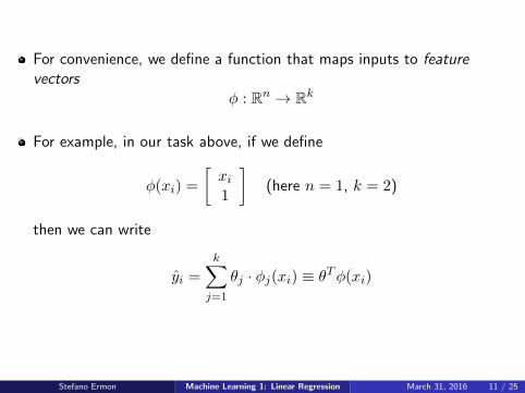
For convenience, we define a function that maps inputs to featurevectors

φ : Rn → Rk

For example, in our task above, if we define

φ(xi) =

[xi1

](here n = 1, k = 2)

then we can write

yi =

k∑j=1

θj · φj(xi) ≡ θTφ(xi)


Loss functions

Want a model that performs “well” on the data we have

I.e., yi ≈ yi, ∀i

We measure “closeness” of yi and yi using loss function

` : R× R→ R+

Example: squared loss

`(yi, yi) = (yi − yi)2


Finding model parameters, and optimization

Want to find model parameters such that minimize sum of costs over allinput/output pairs

J(θ) =

m∑i=1

`(yi, yi) =

m∑i=1

(θTφ(xi)− yi)2

Write our objective formally as

minimizeθ

J(θ)

simple example of an optimization problem; these will dominate ourdevelopment of algorithms throughout the course


How do we optimize a function

Search algorithm: Start with an initial guess for θ. Keep changing θ (bya little bit) to reduce J(θ)

Animation https://www.youtube.com/watch?v=vWFjqgb-ylQ


https://www.youtube.com/watch?v=vWFjqgb-ylQ

Gradient descent

Search algorithm: Start with an initial guess for θ. Keep changing θ (bya little bit) to reduce J(θ)

J(θ) =

m∑i=1

`(yi, yi) =

m∑i=1

(θTφ(xi)− yi)2

Gradient descent: θj = θj − α∂J(θ)∂θj, for all j

∂J

∂θj=∂∑m

i=1(θTφ(xi)− yi)2

∂θj=

m∑i=1

∂(θTφ(xi)− yi)2

∂θj

=

m∑i=1

2(θTφ(xi)− yi)∂(θTφ(xi)− yi)

∂θj

=

m∑i=1

2(θTφ(xi)− yi)φ(xi)j


Gradient descent

Repeat until “convergence”:

θj = θj − αm∑i=1

2(θTφ(xi)− yi)φ(xi)j , for all j

Demo:https://lukaszkujawa.github.io/gradient-descent.html

Stochastic gradient descent


https://lukaszkujawa.github.io/gradient-descent.html

Let’s write J(θ) a little more compactly using matrix notation; define

Φ ∈ Rm×k =

— φ(x1)

T —— φ(x2)

T —...

— φ(xm)T —

, y ∈ Rm =

y1y2...ym

then

J(θ) =

m∑i=1

(θTφ(xi)− yi)2 = ‖Φθ − y‖22

(‖z‖2 is `2 norm of a vector: ‖z‖2 ≡√∑m

i=1 z2i =√zT z)

Called least-squares objective function


How do we optimize a function? 1-D case (θ ∈ R):

−3 −2 −1 0 1 2 3

−2

0

2

4

6

8

10

12

14

−3 −2 −1 0 1 2 3

−2

0

2

4

6

8

10

12

14

−3 −2 −1 0 1 2 3

−8

−6

−4

−2

0

2

4

−3 −2 −1 0 1 2 3

−8

−6

−4

−2

0

2

4

J(θ) = θ2 − 2θ − 1 dJdθ = 2θ − 2

θ? minimum =⇒ dJ

dθ

∣∣∣∣θ?

= 0

=⇒ 2θ? − 2 = 0

=⇒ θ? = 1


Multi-variate case: θ ∈ Rk, J : Rk → R

Generalized condition: ∇θJ(θ)|θ? = 0

∇θJ(θ) denotes gradient of J with respect to θ

∇θJ(θ) ∈ Rk ≡

∂J∂θ1

∂J∂θ2...∂J∂θk

Some important rules and common gradient

∇θ(af(θ) + bg(θ)) = a∇θf(θ) + b∇θg(θ), (a, b ∈ R)

∇θ(θTAθ) = (A+AT )θ, (A ∈ Rk×k)∇θ(bT θ) = b, (b ∈ Rk)


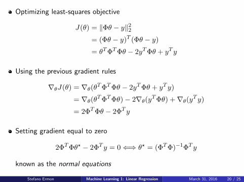
Optimizing least-squares objective

J(θ) = ‖Φθ − y‖22= (Φθ − y)T (Φθ − y)

= θTΦTΦθ − 2yTΦθ + yT y

Using the previous gradient rules

∇θJ(θ) = ∇θ(θTΦTΦθ − 2yTΦθ + yT y)

= ∇θ(θTΦTΦθ)− 2∇θ(yTΦθ) +∇θ(yT y)

= 2ΦTΦθ − 2ΦT y

Setting gradient equal to zero

2ΦTΦθ? − 2ΦT y = 0⇐⇒ θ? = (ΦTΦ)−1ΦT y

known as the normal equations


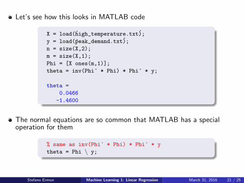
Let’s see how this looks in MATLAB code

X = load(high_temperature.txt);

y = load(peak_demand.txt);

n = size(X,2);

m = size(X,1);

Phi = [X ones(m,1)];

theta = inv(Phi´ * Phi) * Phi´ * y;

theta =

0.0466

-1.4600

The normal equations are so common that MATLAB has a specialoperation for them

% same as inv(Phi´ * Phi) * Phi´ * y

theta = Phi \ y;


Higher-dimensional inputs

Input: x ∈ R2 =

[temperaturehour of day

]

Output: y ∈ R = demand


Features: φ(x) ∈ R3 =

temperaturehour of day

1

Same matrices as before

Φ ∈ Rm×k =

— φ(x1)T —

...— φ(xm)T —

, y ∈ Rm =

y1...ym

Same solution as before

θ ∈ R3 = (ΦTΦ)−1ΦT y


machine learning 1: linear regression - stanford universityermon/cs325/slides/ml_linear_reg.pdf ·...

Documents