ma-207 di erential equations ii - math.iitb.ac.in
TRANSCRIPT

MA-207 Differential Equations II
Ronnie Sebastian
Department of MathematicsIndian Institute of Technology Bombay
Powai, Mumbai - 76
September 19, 2021
1 / 57

Some course policies
Evaluation: 50 marks are waiting to be earned:
Quiz 20 marksEnd Semester exam 30 marksTotal 50 marks
The quiz will be held in the tutorial on 12th October, 2021.
FR grade if marks are < 15/50.
Any form of academic dishonesty will invite severe penalties.
2 / 57

Books
Elementary differential equations with boundary value problemsby William F. Trench (available online)
Differential Equations with Applications and Historical Notesby George F. Simmons
3 / 57

Aim of this course
The aim of this course is to see some methods to find solutions todifferential equations.
There are two parts in this course.
1 In the first part we shall see how to solve differential equationsin one variable.
2 In the second part we shall see how to solve differentialequations involving functions of two variables.
In both parts we shall find solutions to the differential equations asseries.
In the first part, these series will usually be power series in onevariable. In the second part, we will consider more complicatedkinds of series, for example, Fourier series.
4 / 57

Aim of this course
A very beautiful, simple and powerful technique we will learn inthis course is the Method of Separation of Variables. This willcome towards the end of the course.
Separation of variables, combined with the series representation,yields a way to solve some PDE’s, which otherwise will beincredibly hard to solve.
For example, try to solve the following PDE (heat equation) onyour own
ut = k2uxx 0 < x < L, t > 0
u(0, t) = 0 t ≥ 0
u(L, t) = 0, t ≥ 0
u(x, 0) = x(L− x), 0 ≤ x ≤ LMore generally, instead of x(L− x) we could have taken any“nice” function. We will learn in the last few lectures how to solvethis PDE. This ends a very brief introduction and we now beginthe course with a study of power series.
5 / 57

Power Series
Consider an ODE
y′′ + p(x)y′ + q(x)y = 0
with p(x), q(x) continuous.
Let y1(x) be one solution of the above ODE.
We can try to use the method of variation of parameters to findanother linearly independent solution, that is, put
y2(x) = u(x)y1(x)
in the ODE and solve for u(x).
Question. How to find one solution?
For this, we will solve our ODE in terms of power series.
6 / 57

Power Series
Definition
For real numbers x0, a0, a1, a2, . . ., an infinite series
∞∑n=0
an(x− x0)n := a0 + a1(x− x0) + a2(x− x0)2 + . . . .
is called a power series in x− x0 with center x0.
For a real number x1, if the limit
limN→∞
N∑n=0
an(x1 − x0)n
exists and is finite, then we say the power series converges at thepoint x = x1.In this case, the value of the series at x1 is, by definition, the valueof the limit.
7 / 57

Power series
Definition
If the series does not converge at x1, that is, either the limit doesnot exist, or it is ±∞, then we say the power series diverges at x1.
Obviously, a power series always converges at its center x = x0.
8 / 57

Power series - Radius of convergence
Theorem
For any power series,
∞∑n=0
an(x− x0)n
exactly one of these statements is true.
1 The power series converges only for x = x0.
2 The power series converges for all values of x.
3 There is a positive number 0 < R <∞ such that the powerseries converges if |x− x0| < R and diverges if |x− x0| > R.
R is called the radius of convergence of the power series.
Define R = 0 in case (i)Define R =∞ in case (ii).
9 / 57

Power Series - Radius of convergence
Question. How to compute the radius of convergence?
There are two methods to do this.
Theorem
(Ratio test) Assume that there is an integer N such that for alln ≥ N we have an 6= 0. Also assume the following limit exists
limn→∞
∣∣∣∣an+1
an
∣∣∣∣and denote it by L.
Then radius of convergence of the power series∞∑n=0
an(x− x0)n is
R = 1/L .
For L = 0, we get R =∞and for L =∞, we get R = 0.
10 / 57

Power series - Radius of convergence
The ratio test will not work for all series (for example, when manyof the an’s are 0).
However, the root test, which is the second method to computethe radius of convergence, will work for all power series. We firstneed to recall the definition of limsup.
Definition
Suppose we are given a sequence {an}n≥1.For every k ≥ 1 define
bk := supn≥k{an} .
Convince yourself that {bk}k≥1 is a decreasing sequence, that is,
b1 ≥ b2 ≥ b3 ≥ . . .
Definelim sup{an} := limn→∞bn .
11 / 57

Power series - Radius of convergence
Definition
Similarly, define lim inf{an}, by replacing sup by inf in the abovediscussion.
Remark
Note that for a sequence {an}n≥1, the limit may not exist.However, the lim sup and lim inf always exist (possibly +∞ or−∞).
Theorem
Let {an}n≥1 be a sequence of real numbers. Then limn→∞anexists if and only if lim sup{an} = lim inf{an}.Further, if limn→∞an exists, then
lim sup{an} = lim inf{an} = limn→∞an
12 / 57

Power series - Radius of convergence
Strictly speaking, when we say that limn→∞an exists, we meanthat this limit exists and is finite.
However, sometimes we shall be a little careless and say thatlimn→∞an exists in the following cases also: if limn→∞an =∞ orlimn→∞an = −∞.
Recall, for example, the definition of limn→∞an =∞. For everyN ∈ R, there exists n(N) ≥ 1 (that is, n depends on N) such thatak ≥ N for all k ≥ n(N).
For example, convince yourself that for the sequence defined byb2n−1 := n and b2n := n− 1 (n ≥ 1), we have limn→∞bn =∞
13 / 57

Power series - Radius of convergence
Now that we have recalled the definition of limsup, we return tothe root test.
Theorem
(Root test)Let lim sup{|an|1/n} = L.
Then radius of convergence of the power series∞∑n=0
an(x− x0)n is
R = 1/L .
For L = 0, we get R =∞.For L =∞, we get R = 0.
This concludes the discussion on how to compute the radius ofconvergence of a power series.
14 / 57

Power series - Radius of convergence
Theorem
Let R > 0 be the radius of convergence of the power series
∞∑n=0
an(x− x0)n
Then the power series converges (absolutely) for allx ∈ (x0 −R, x0 +R).
For R =∞, we write (x0 −R, x0 +R) = (−∞,∞) = R.
Definition
The open interval (x0 −R, x0 +R) is called the interval ofconvergence of the power series.
15 / 57

Power series - examples
Example
Find the radius of convergence and interval of convergence (ifR > 0) of
∞∑0
n!xn .
limn→∞
∣∣∣∣an+1
an
∣∣∣∣ = limn→∞
∣∣∣∣(n+ 1)!
n!
∣∣∣∣ = limn→∞
(n+ 1) =∞ .
So R = 1/∞ = 0.
16 / 57

Power series - examples
Example
Find the radius of convergence and interval of convergence (ifR > 0) of
∞∑10
(−1)nxn
nn
limn→∞
∣∣∣∣an+1
an
∣∣∣∣ = limn→∞
∣∣∣∣ nn
(n+ 1)n+1
∣∣∣∣ = 0
So R = 1/0 =∞. Interval of convergence (−∞,∞).
17 / 57

Power series - examples
Example
Find the radius of convergence and interval of convergence (ifR > 0) of
∞∑0
2nn3(x− 1)n
limn→∞
∣∣∣∣an+1
an
∣∣∣∣ = limn→∞
∣∣∣∣2n+1(n+ 1)3
2nn3
∣∣∣∣ = 2
So R = 1/2. Interval of convergence (1/2, 3/2).
18 / 57

Power series as functions
Theorem
Let R be the radius of convergence of the power series∞∑n=0
an(x− x0)n. We assume R > 0 .
We define a function f : (x0 −R, x0 +R)→ R by
f(x) =
∞∑n=0
an(x− x0)n
This function satisfies the following properties
1 f is infinitely differentiable ∀ x ∈ (x0 −R, x0 +R).
19 / 57

Power series as functions
Theorem (continued . . .)
2 The successive derivatives of f can be computed bydifferentiating the power series term-by-term, that is,
f ′(x) =d
dx
∞∑n=0
an(x− x0)n
=
∞∑n=0
d
dxan(x− x0)n
Exchanging a differential operator and a sum/integral issomething which needs to be done with care
=
∞∑n=0
nan(x− x0)n−1
20 / 57

Power series as functions
Theorem (continued . . .)
3 f (k)(x) =
∞∑n=0
n(n− 1) . . . (n− k + 1) an(x− x0)n−k
4 The power series representing the derivatives f (n)(x) havesame radius of convergence R.
5 We can determine the coefficients an (in terms of derivativesof f at x0) as
an =f (n)(x0)
n!
21 / 57

Power series as functions
Theorem (continued . . .)
• We can also integrate the function f(x) =∞∑0
an(x− x0)n
term-wise, that is,if [a, b] ⊂ (x0 −R, x0 +R), then∫ b
af(x) dx =
∞∑n=0
an
∫ b
a(x− x0)n dx =
∞∑0
ann+ 1
(x− x0)n+1
Exchanging an integral operator and a sum is something whichneeds to be done with care
22 / 57

Power series as functions
Theorem
(i) Power series representation of f in an open interval Icontaining x0 is unique, that is, if
f(x) =
∞∑0
an(x− x0)n =
∞∑0
bn(x− x0)n
for all x ∈ I, then an = bn ∀ n.(ii) If
∞∑0
an(x− x0)n = 0
for all x ∈ I, then an = 0 for all n.
Proof. (i)
an =f (n)(x0)
n!= bn for all n.
It is clear that (ii) follows from (i).23 / 57

Examples of power series
Example (Power series representation of some familiar functions)
(i) ex =
∞∑0
xn
n!−∞ < x <∞
(ii) sinx =
∞∑0
(−1)n x2n+1
(2n+ 1)!−∞ < x <∞
(iii)1
1− x=∞∑0
xn − 1 < x < 1
(iv)d
dx(sinx) =
∞∑0
(−1)n d
dx
(x2n+1
(2n+ 1)!
)
=∞∑0
(−1)n x2n
(2n)!= cosx
24 / 57
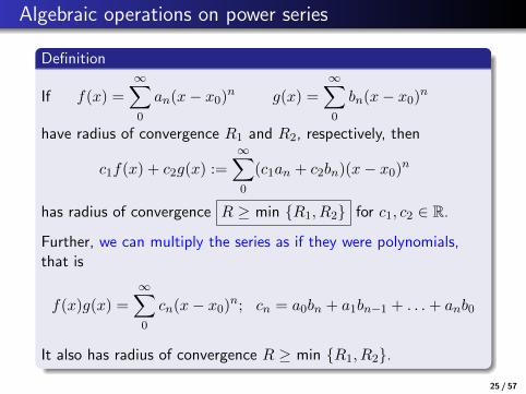
Algebraic operations on power series
Definition
If f(x) =
∞∑0
an(x− x0)n g(x) =
∞∑0
bn(x− x0)n
have radius of convergence R1 and R2, respectively, then
c1f(x) + c2g(x) :=
∞∑0
(c1an + c2bn)(x− x0)n
has radius of convergence R ≥ min {R1, R2} for c1, c2 ∈ R.
Further, we can multiply the series as if they were polynomials,that is
f(x)g(x) =
∞∑0
cn(x− x0)n; cn = a0bn + a1bn−1 + . . .+ anb0
It also has radius of convergence R ≥ min {R1, R2}.
25 / 57

Algebraic operations on power series
Example
Find the power series expansion for coshx in terms of powers ofxn.
coshx =1
2ex +
1
2e−x
=1
2
∞∑n=0
xn
n!+
1
2
∞∑n=0
(−1)nxn
n!
=
∞∑n=0
1
2[1 + (−1)n] x
n
n!
=∞∑n=0
x2n
(2n)!
Since radius of convergence for Taylor series of ex and e−x are ∞,the power series expansion of coshx is valid on R.
26 / 57

Algebraic operations on power series
If f(x) =∞∑n=0
an(x− x0)n then f ′(x) =∞∑n=1
nan(x− x0)n−1.
Put r = n− 1 into f ′(x), we get
f ′(x) =
∞∑r=0
(r + 1)ar+1(x− x0)r
Similarly,
f (k)(x) =
∞∑n=k
n(n− 1) . . . (n− k + 1)an(x− x0)n−k
=
∞∑n=0
(n+ k)(n+ k − 1) . . . (n+ 1)an+k(x− x0)n
27 / 57

Algebraic operations on power series
Example
Let f(x) =∞∑n=0
anxn. Write (x− 1)f ′′ as a power series around 0.
(x− 1)f ′′ = xf ′′ − f ′′
= x
( ∞∑n=2
n(n− 1)anxn−2
)−∞∑n=2
n(n− 1)anxn−2
=
∞∑n=2
n(n− 1)anxn−1 −
∞∑n=2
n(n− 1)anxn−2
=
∞∑n=1
(n+ 1)nan+1xn −
∞∑n=0
(n+ 2)(n+ 1)an+2xn
=∞∑n=0
[(n+ 1)nan+1 − (n+ 2)(n+ 1)an+2]xn
�
28 / 57

Using power series to find formal solution to ODE’s
Example
Suppose
y(x) =
∞∑n=0
an(x− 1)n
for all x in an open interval I containing x0 = 1.
Find the power series of y′ and y′′ in terms of x− 1 in theinterval I. Use these to express the function
(1 + x)y′′ + 2(x− 1)2y′ + 3y
as a power series in x− 1 on I.
Find necessary and sufficient conditions on the coefficientsan’s, so that y(x) is a formal solution of the ODE
(1 + x)y′′ + 2(x− 1)2y′ + 3y = 0
29 / 57

Using power series to find formal solution to ODE’s
Example (continued . . .)
Solution. Write the ODE in (x− 1), that is
(1 + x)y′′+2(x− 1)2y′+3y = (x− 1)y′′+2y′′+2(x− 1)2y′+3y
Express each of (x− 1)y′′, 2y′′, 2(x− 1)2y′ and 3y as a powerseries in powers of (x− 1) and add them.
(x− 1)y′′ = (x− 1)
∞∑n=2
n(n− 1)an(x− 1)n−2
=
∞∑n=2
n(n− 1)an(x− 1)n−1
=
∞∑n=1
(n+ 1)nan+1(x− 1)n
=
∞∑n=0
(n+ 1)nan+1(x− 1)n
30 / 57

Using power series to find formal solution to ODE’s
Example (continued . . .)
2y′′ =
∞∑n=2
2n(n− 1)an(x− 1)n−2
=
∞∑n=0
2(n+ 2)(n+ 1)an+2(x− 1)n
2(x− 1)2y′ = 2(x− 1)2∞∑n=1
nan(x− 1)n−1
=
∞∑n=1
2nan(x− 1)n+1
=∞∑n=2
2(n− 1)an−1(x− 1)n
=∞∑n=0
2(n− 1)an−1(x− 1)n (a−1 = 0)
31 / 57

Using power series to find formal solution to ODE’s
Example (continued . . .)
We have
(x− 1)y′′ =
∞∑n=0
(n+ 1)nan+1(x− 1)n
2y′′ =
∞∑n=0
2(n+ 2)(n+ 1)an+2(x− 1)n
2(x− 1)2y′ =
∞∑n=0
2(n− 1)an−1(x− 1)n (a−1 = 0)
Now we get
(x− 1)y′′ + 2y′′ + 2(x− 1)2y′ + 3y =∞∑n=0
bn(x− 1)n
where
bn = (n+ 1)nan+1 + 2(n+ 2)(n+ 1)an+2 + 2(n− 1)an−1 + 3an
32 / 57
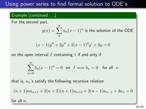
Using power series to find formal solution to ODE’s
Example (continued . . .)
For the second part,
y(x) =
∞∑0
an(x− 1)n is the solution of the ODE
(x− 1)y′′ + 2y′′ + 2(x− 1)2y′ + 3y = 0
on the open interval I containing 1 if and only if
∞∑n=0
bn(x− 1)n = 0 on I ⇐⇒ bn = 0 for all n
that is, an’s satisfy the following recursive relation
(n+ 1)nan+1 + 2(n+ 2)(n+ 1)an+2 + 2(n− 1)an−1 + 3an = 0
for all n.33 / 57
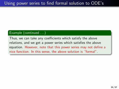
Using power series to find formal solution to ODE’s
Example (continued . . .)
Thus, we can take any coefficients which satisfy the aboverelations, and we get a power series which satisfies the aboveequation. However, note that this power series may not define anice function. In this sense, the above solution is “formal”.
34 / 57

Taylor series
Definition
Let f(x) be an infinitely differentiable at x0. The Taylor series off at x0 is defined as the power series
TS f |x0 :=
∞∑0
f (n)(x0)
n!(x− x0)n
Let us make an observation.
Suppose f is defined by a power series in an interval of x0, that is,f(x) =
∑n≥0 an(x− x0)n in the interval (x0 −R, x0 +R). When
we apply the above definition of Taylor series, we see that
TSf |x0 =
∞∑0
an(x− x0)n = f(x) .
Thus, in this case from the Taylor series we get back the functionf .
35 / 57

Taylor series
However, the class of infinitely differentiable functions is largerthan the class of power series and the above need not be true forinfinitely differentiable functions in an interval around x0
Example
The function f(x) =
{e−1/x
2if x 6= 0
0 if x = 0
is infinitely differentiable at 0. But f (n)(0) = 0 for all n.
Hence the Taylor series of f at 0 is the constant function takingvalue 0.
Therefore Taylor series of f at 0 does not converge to functionf(x) on any open interval around 0.
36 / 57

Taylor series
Definition
Suppose
f(x) is infinitely differentiable at x0; and
Taylor series of f at x0 converges to f(x) for all x in someopen interval around x0;
Then f is called analytic at x0.
Thus, if f is analytic, then there is an interval I around x0 and fis given by a power series in I.
Example
The function f(x) =
{e−1/x
2if x 6= 0
0 if x = 0is not analytic at 0. Here 2nd condition fails. However, f isanalytic at all x 6= 0.
37 / 57

Analytic functions
Example
1 Polynomials, ex, sinx and cosx are analytic at all x ∈ R.
2 f(x) = tanx is analytic at all x except x = (2n+ 1)π/2,where n = ±1,±2, . . ..
3 f(x) = x5/3 is analytic at all x except x = 0.
38 / 57

Analytic functions
Theorem (Analytic functions)
1 If f(x) and g(x) are analytic at x0, thenf(x)± g(x) f(x)g(x) f(x)/g(x) (if g(x0) 6= 0)are analytic at x0.
2 If f(x) is analytic at x0 and g(x) is analytic at f(x0), theng(f(x)) := (g ◦ f)(x) is analytic at x0.
3 If a power series∞∑0
an(x− x0)n has radius of convergence
R > 0, then the function f(x) :=∞∑0
an(x− x0)n
is analytic at all points x ∈ (x0 −R, x0 +R).
39 / 57

Analytic functions
Example
The function f(x) = x2 + 1 is analytic everywhere. Since x2 + 1 isnever 0, the function h(x) := 1
x2+1is analytic everywhere.
However, there is no power series around 0 which represents h(x)on R.
If there were such a power series, then by uniqueness, it has to bethe power series expansion of h(x) around 0, which is
1− x2 + x4 − x6 + · · ·
However, the radius of convergence of this is R = 1.
In fact, for any x0, there is no power series around x0 whichrepresents h(x) everywhere.
40 / 57

Analytic functions
Theorem
Let
F (x) =N(x)
D(x)example F (x) =
x3 − 1
x2 + 1
be a rational function, where N(x) and D(x) are polynomialswithout any common factors, that is they do not have anycommon (complex) zeros. Let α1, . . . , αr be distinct complex zerosof D(x).
Then F (x) is analytic at all x except at x ∈ {α1, . . . , αr}.If x0 isdifferent from {α1, . . . , αr}, then the radius of convergence R ofthe Taylor series of F at x0
TS Fx0 =
∞∑0
F (n)(x0)
n!(x− x0)n
41 / 57

Analytic functions
Theorem (continued . . . )
is given by
R = min {|x0 − α1|, |x0 − α2|, . . . , |x0 − αr|}
42 / 57

Analytic functions
Example
If
F (x) =N(x)
D(x)=
(2 + 3x)
(4 + x)(9 + x2)
then D(x) has zeros at −4 and ±3ι, where ι =√−1.
Hence F is analytic at all x except at x ∈ {−4,±3ι}.If x = 2, then radius of convergence of Taylor series of F at x = 2is
min {|2 + 4|, |2 + 3ι|, |2− 3ι|} = min {6,√13} =
√13
If x = −6, then radius of convergence of Taylor series of F atx = −6 is
min {| − 6 + 4|, | − 6± 3ι|} = min {2,√45} = 2
43 / 57

Power series solution of ODE
Theorem (Existence Theorem)
If p(x) and q(x) are analytic functions at x0, then every solution of
y′′ + p(x)y′ + q(x)y = 0
is also analytic at x0; and therefore any solution can be expressedas
y(x) =
∞∑0
an(x− x0)n
If R1 = radius of convergence of Taylor series of p(x) at x0,
R2 = radius of convergence of Taylor series of q(x) at x0,
then radius of convergence of y(x) is at least min(R1, R2) > 0.
In most applications, p(x) and q(x) are rational functions, that isquotient of polynomial functions.
44 / 57

Power series solution of ODE
Example
Let us solve y′′ + y = 0 (1) by power series method.
Compare with y′′ + p(x)y′ + q(x)y = 0,p(x) = 0 and q(x) = 1 are analytic at all x.We can find power series solution in x− x0 for any x0.Let us assume x0 = 0 for simplicity.By existence theorem, all solution of (1) can be found in the form
y(x) =
∞∑0
anxn
and the series will have ∞ radius of convergence.Since
y′′ =∞∑2
n(n− 1)anxn−2 =
∞∑n=0
(n+ 2)(n+ 1)an+2xn
45 / 57

Power series solution of ODE
Example (Continue . . .)
y′′ + y =
∞∑0
((n+ 2)(n+ 1)an+2 + an)xn = 0
By uniqueness of power series in x− x0 we get the recursionformula
(n+ 2)(n+ 1)an+2 + an = 0
=⇒ an+2 =−1
(n+ 2)(n+ 1)an ∀n
Therefore,
a2 =−12.1
a0, a4 =−14.3
a2 =1
4!a0 . . . a2n = (−1)n 1
(2n)!a0
a3 =−13.2
a1, a5 =−15.4
a3 =1
5!a1 . . . a2n+1 = (−1)n 1
(2n+ 1)!a1
46 / 57

Power series solution of ODE
Example (Continue . . .)
Define
y1(x) = 1− 1
2!x2 +
1
4!x4 − . . . (a0 = 1, a1 = 0)
y2(x) = x− 1
3!x3 +
1
5!x5 − . . . (a0 = 0, a1 = 1)
Then
y(x) =
∞∑0
anxn = a0y1(x) + a1y2(x)
is a general solution of the ODE (1).
In this case, y1(x) = cosx and y2(x) = sinx.We don’t need to check the series for converges, since theexistence theorem guarantees that the series converges for all x.
47 / 57

Power series solution of ODE
In this course, we will consider ODE
P0(x)y′′ + P1(x)y
′ + P2(x)y = 0
with Pi(x) polynomials for i = 0, 1, 2 without any common factor.If we write ODE in the standard form
y′′ +P1(x)
P0(x)y′ +
P2(x)
P0(x)y = 0
and if x0 is not a zero of P0(x), then P1(x)/P0(x) andP2(x)/P0(x) will be analytic at x0, hence, we can find the seriessolution of ODE in the form
y(x) =
∞∑0
an(x− x0)n
48 / 57

Power series solution of ODE
Steps for Series solution of linear ODE
1 Write ODE in standard form y′′ + p(x)y′ + q(x)y = 0.
2 Choose x0 at which p(x) and q(x) are analytic. If boundaryconditions at x0 are given, choose the center of the powerseries as x0.
3 Find minimum of radius of convergence of Taylor series ofp(x) and q(x) at x0.
4 Let y(x) =∞∑0
an(x− x0)n, compute the power series for
y′(x) and y′′(x) at x0 and substitute these into the ODE.
5 Set the coefficients of (x− x0)n to zero and find recursionformula.
6 From the recursion formula, obtain (linearly independent)solutions y1(x) and y2(x). The general solution then lookslike y(x) = a1y1(x) + a2y2(x).
49 / 57

Power series solution of ODE
Example
Find the power series in x for the general solution of
(1 + 2x2)y′′ + 6xy′ + 2y = 0
Solution. Note that 0 is not a zero of P0(x) = 1+ 2x2, hence, theseries solution in powers of x exists.
Putting y =∞∑0
anxn in the ODE, we get
(1 + 2x2)y′′ + 6xy′ + 2y
= y′′ + 2x2y′′ + 6xy′ + 2y
=
∞∑0
((n+ 2)(n+ 1)an+2 + 2n(n− 1)an + 6nan + 2an)xn
=⇒ (n+ 2)(n+ 1)an+2 + [2n(n− 1) + 6n+ 2]an = 0
50 / 57
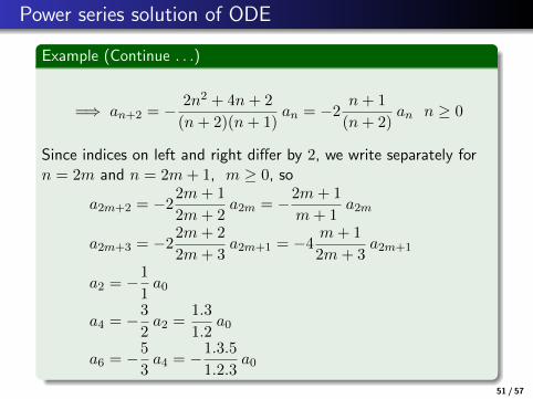
Power series solution of ODE
Example (Continue . . .)
=⇒ an+2 = −2n2 + 4n+ 2
(n+ 2)(n+ 1)an = −2 n+ 1
(n+ 2)an n ≥ 0
Since indices on left and right differ by 2, we write separately forn = 2m and n = 2m+ 1, m ≥ 0, so
a2m+2 = −22m+ 1
2m+ 2a2m = −2m+ 1
m+ 1a2m
a2m+3 = −22m+ 2
2m+ 3a2m+1 = −4
m+ 1
2m+ 3a2m+1
a2 = −1
1a0
a4 = −3
2a2 =
1.3
1.2a0
a6 = −5
3a4 = −
1.3.5
1.2.3a0
51 / 57
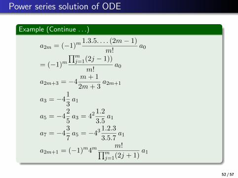
Power series solution of ODE
Example (Continue . . .)
a2m = (−1)m 1.3.5. . . . (2m− 1)
m!a0
= (−1)m∏m
j=1(2j − 1))
m!a0
a2m+3 = −4m+ 1
2m+ 3a2m+1
a3 = −41
3a1
a5 = −42
5a3 = 42
1.2
3.5a1
a7 = −43
7a5 = −43
1.2.3
3.5.7a1
a2m+1 = (−1)m4mm!∏m
j=1(2j + 1)a1
52 / 57

Power series solution of ODE
Example (continued . . .)
We can write the solution
y =
∞∑0
anxn = a0y1(x) + a1y2(x)
where a0 and a1 are arbitrary scalars and
y1(x) =
∞∑m=0
(−1)m∏m
j=1(2j − 1)
m!x2m
y2(x) =
∞∑m=0
(−1) 4mm!∏mj=1(2j + 1)
x2m+1
Since P0(x) = 1 + 2x2 has complex zeros±ι√2
, the power series
solution converges in the interval
(−1√2,1√2
). �
53 / 57
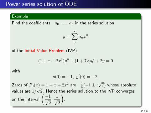
Power series solution of ODE
Example
Find the coefficients a0, . . . , a6 in the series solution
y =
∞∑0
anxn
of the Initial Value Problem (IVP)
(1 + x+ 2x2)y′′ + (1 + 7x)y′ + 2y = 0
withy(0) = −1, y′(0) = −2.
Zeros of P0(x) = 1 + x+ 2x2 are 14(−1± ι
√7) whose absolute
values are 1/√2. Hence the series solution to the IVP converges
on the interval
(−1√2,1√2
).
54 / 57

Power series solution of ODE
Example (continued . . .)
(1 + x+ 2x2)y′′ + (1 + 7x)y′ + 2y =
∞∑0
bnxn = 0
bn = (n+ 2)(n+ 1)an+2 + (n+ 1)nan+1 + 2n(n− 1)an
+(n+ 1)an+1 + 7nan + 2an = 0
that is
(n+ 2)(n+ 1)an+2 + (n+ 1)2an+1 + (2n2 + 5n+ 2)an = 0
Since 2n2 + 5n+ 2 = (n+ 2)(2n+ 1),
an+2 = −n+ 1
n+ 2an+1 −
2n+ 1
n+ 1an n ≥ 0
55 / 57

Power series solution of ODE
Example (continued . . .)
an+2 = −n+ 1
n+ 2an+1 −
2n+ 1
n+ 1an n ≥ 0
From the initial conditions y(0) = −1, y′(0) = −2 we get
a0 = y(0) = −1, a1 = y′(0) = −2
a2 = −1
2a1 − a0 = 2
a3 = −2
3a2 −
3
2a1 =
5
3
Check that
y(x) = −1− 2x+ 2x2 +5
3x3 − 55
12x4 +
3
4x5 +
61
8x6 + . . .
56 / 57

Slightly more complicated ODE’s
The best possible situation is when we have an ODE of the form
y′′ + p(x)y′ + q(x) = 0
where p(x) and q(x) are analytic in an interval around x0.
We just saw how to solve such ODE’s.
We will next consider in detail the Legendre equation (an ODEwhich falls in the above category of “nice” ODE’s)
(1− x2)y′′ − 2xy′ + α(α+ 1)y = 0 .
However, there are other ODE’s which occur naturally, which donot fall into the above “nice” category, and which we would like tosolve. For example, Bessel’s equation :
x2y′′ + xy′ + (x2 − ν2)y = 0
We will see later how to solve some such ODE’s.57 / 57