m 13676 supplement 1 use - int-res.com

Supplement to Weigel et al. (2021) – Mar Ecol Prog Ser 666:135-‐148 – https://doi.org/10.3354/meps13676

1

Supplement 1

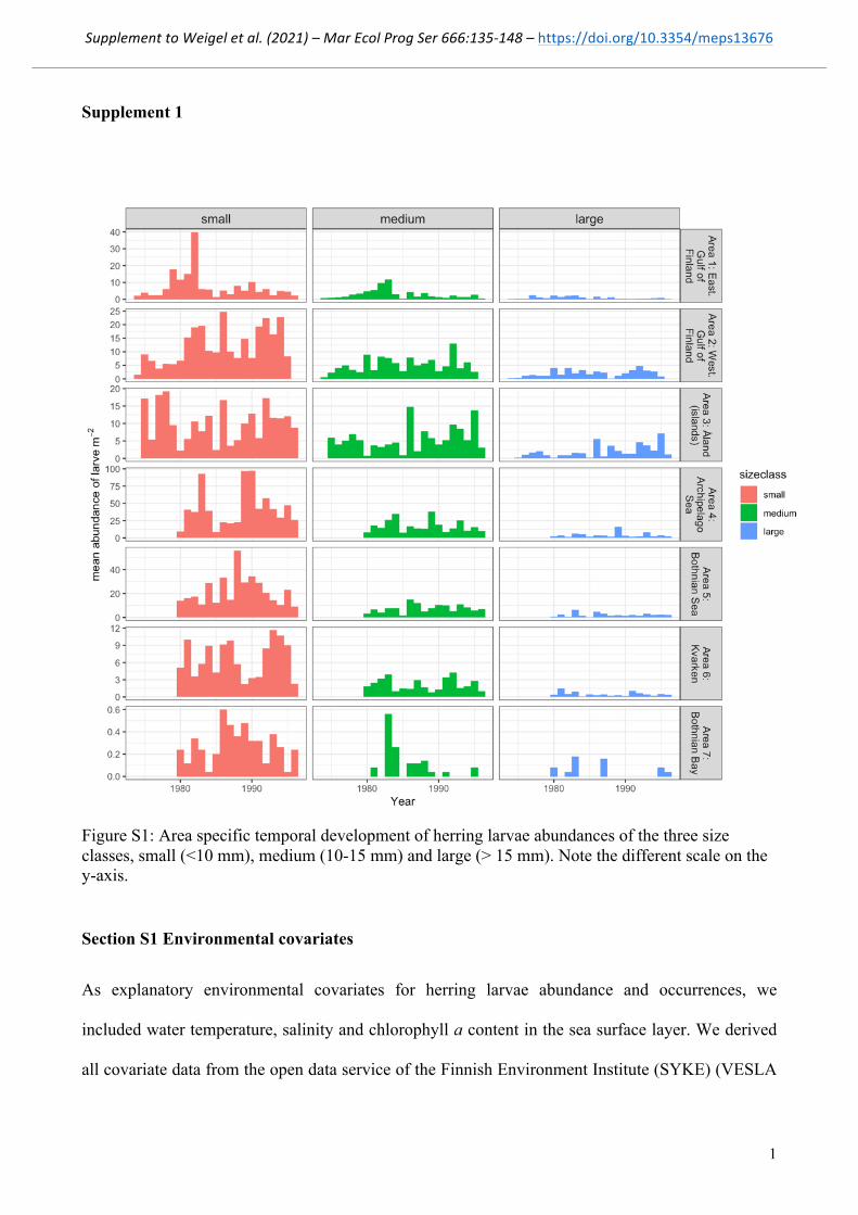
Figure S1: Area specific temporal development of herring larvae abundances of the three size classes, small (<10 mm), medium (10-15 mm) and large (> 15 mm). Note the different scale on the y-axis.

Section S1 Environmental covariates

As explanatory environmental covariates for herring larvae abundance and occurrences, we

included water temperature, salinity and chlorophyll a content in the sea surface layer. We derived

all covariate data from the open data service of the Finnish Environment Institute (SYKE) (VESLA


2

/ reference: the Finnish Environment Institute and the Centres for Economic Development,

Transport and the Environment / accessed through http://rajapinnat.ymparisto.fi/api/vesla/2.0/

SYKE; Baltic Environmental Database / reference: Baltic Nest Institute / accessed through

http://rajapinnat.ymparisto.fi/api/veslabnirajapinta/1.0/), and for surface temperature also from

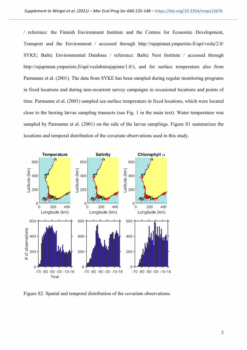
Parmanne et al. (2001). The data from SYKE has been sampled during regular monitoring programs

in fixed locations and during non-recurrent survey campaigns in occasional locations and points of

time. Parmanne et al. (2001) sampled sea surface temperature in fixed locations, which were located

close to the herring larvae sampling transects (see Fig. 1 in the main text). Water temperature was

sampled by Parmanne et al. (2001) on the side of the larvae samplings. Figure S1 summarizes the

locations and temporal distribution of the covariate observations used in this study.

Figure S2. Spatial and temporal distribution of the covariate observations.


3

We derived covariate maps by interpolating the observations with a spatio-temporal statistical

model. We built models for each covariate and predicted the covariate value for study areas. For the

predictions, we discretized the study areas into grids, which varied by area from 60 km2 to 90 km2,

and had a 10 km x 10 km resolution. We predicted the covariate values in the center points of the

grid cells. The cell size was set so that point wise predictions would catch the expected spatial

variation between cells. Observations were located quite densely so that the minimum distance

between observations was less than a kilometer for each covariate. The estimates for the spatial

scales of the model functions varied from less than 3 km to over 500 km. Table S2 shows the

estimates of each function’s parameters and Table S3 shows the relative importance of each

function. By comparing the estimated spatial correlation length of the spatial model components

with the importance of the components we can notice that 10 km spatial resolution for the

prediction grid well captured the variation of the model components. Lastly, we took the average

over the prediction points specifically for each study area.

Covariates were predicted firstly for fitting the larvae models in the same sampling occasions when

larvae were sampled in the months from May to August throughout the study period. The in-situ

observations of covariates from SYKE covered the years 1970-2018. The water temperature data

from Parmanne et al. (2001) covered the years 1974-1996.

Due to the computational constraints of the inference for the spatiotemporal models, we restricted

the number of observations to 10 000. This many observations were used for inferring the values of

unknown parameters of the spatial, and spatiotemporal covariance functions. For water temperature,

we prioritized the observations from Parmanne et al. (2001), which made already 5,350

observations. In Åland study area, we used a 50 km search radius for observations around the study

area for all covariates, because the Åland archipelago is less intensively sampled than other coastal

areas. For all other areas, we used a 15 km search radius around the study areas. For water

temperature we could derive enough observations from inside the other study areas to reach the


4

10,000 observations without a need to widen the search outside of the study areas. Most of the

observations are from the open sea season, from April to November.

For predicting covariate values, the computational burden is less intensive than in fitting the

covariate functions. Thus, we derived 15,000 observations for each covariate for predicting, which

provides us with more information about the environmental conditions.

Spatio-temporal model for environmental covariates

The spatiotemporal models for environmental covariates were constructed with Gaussian Processes

(GPs), which define latent values continuously over the study area (Rasmussen & Williams, 2006).

GP regression can be applied for inferring model parameters and predicting latent value in new data

points (Banerjee, Gelfand, & Carlin, 2015). Here we defined the spatiotemporal model separately

for each covariate with additive GPs so that

!! = ! + !!(!!)+ !!!!(!!)+ ! !! , !! + ℎ !! , !! + !!, (1)

where ! is the covariate value, ! is an index of samples, ! is the model intercept (modeling the

average covariate value over the data set), !! is a spatially varying constant term, !! is the time

stamp of the observation, !! is a spatially varying linear temporal trend, ! is a non-periodic

spatiotemporal random effect describing spatiotemporally correlated residuals, ℎ is a periodic

spatiotemporal random effect describing annual seasonality in the covariate values and ! is an

independent random error. The study areas cover a spatially long climatic gradient, which means

that average environmental conditions vary between areas. This is accounted for by spatially

varying constant term (!!) and linear temporal trend (!!!!). The spatially varying linear temporal

trend models the temporal change over the study period assuming spatial variation in the slope

parameter. We assume also that covariates may correlate in longer spatial ranges than around 100


5

km, which is the maximum distance inside the study areas widened with search radius. Thus, we

model the spatiotemporal dependence in ! and ℎ between all observations.

We inferred the correlation parameters of spatial, spatio-temporal and residual error functions in a

hierarchical Bayesian framework (Wikle, 2003).

Structure of the random effects

We gave zero mean Gaussian process (GP) priors for each random effect in the model

!! ! ~!" 0, !!! !, !! !!! , (3)

!! ! ~!" 0, !!! !, !! !!! , (4)

ℎ !, ! ~!"(0, !! !, ! , !!, !! !! , (5)

! !, ! ~!"(0, !! !, ! , !!, !! !! , (6)

where ! denotes the covariance function parameters. Both !!! and !!!, were defined as Matérn

functions with 3/2 degrees of freedom

!!!( ! , !! ) = !!!

! 1+ 3!!! exp − 3!!! , (7)

!!!( ! , !! ) = !!!

! 1+ 3!!! exp − 3!!! , (8)

where !!!! and !!!

! control the magnitudes of variation and contribute to the strength of effect of the

respective function on the latent value, and !!!and !!! are parameterized similarly so that

!!! = !! − !!! !/!!!!! !

!!! , where further !!!!! contributes to the smoothness of variation so that

small values create quick changes of the random effect and large values create smooth changes. The

covariance structure of the spatially varying linear temporal trend is defined as

!"#[!!! ! , !′!! !! ] = !!!!!!(!, !!), (9)


6

which returns the covariance of temporally weighted spatial random effect (see, e.g., (Mäkinen &

Vanhatalo, 2016) for more discussion on spatially varying coefficient models). For !! ! !! ! ,

we assigned separate lengthscales (!!!!! , !!!!

! ) for x- and y-coordinates. Thus, we assumed that the

spatial correlation length may differ between latitudinal and longitudinal directions.

Spatiotemporal covariance functions were constructed by taking a product of spatial and temporal

correlations. The spatial parts of !! and !! were modeled with a Matérn type covariance function

with 3/2 degrees of freedom. The temporal part of !! was modeled with an exponential covariance

function and of !! with a periodic covariance function. The products of the spatial and temporal

covariance functions are defined as

!!( !, ! , !!, !! ) = !!! 1+ 3!! exp − 3!! exp (− !!!!

!!!), (10)

!! !, ! , !!, !! = !!! 1+ 3!! exp − 3!! exp −

!!!!

!

!!!!"#$%! −

! !"#!(! !!!!

! )

!!!! ,

(11)

where !! and !! are parameterized similarly so that !! = !! − !!! !/!!!!!!!! . In the periodic

covariance function (11), ! is the periodicity of the temporal covariance. We fixed it to a year to

represent the annual cycle of the environmental covariates but allowed the periodic random effect

decay from exact periodicity by adding a squared exponential part in the covariance function (see

(Rasmussen & Williams, 2006)). Thus, the periodic pattern may vary during the study period. This

variance is expected to be slow compared to the other temporal patterns and hence we gave, !!!"#$%

such prior, which prefers long length scales (see Table S1).

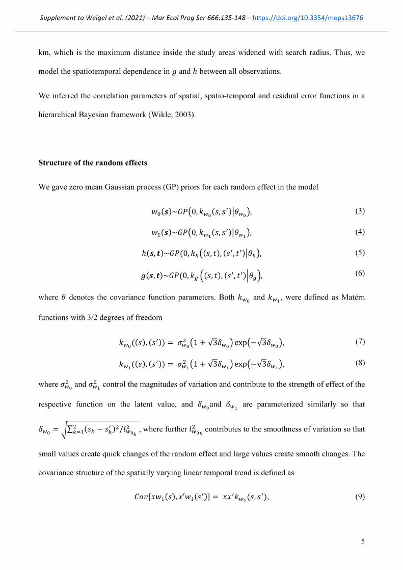
We assigned same a priori weight for all functions through variance parameters (Table S1). We

preferred slower decay of correlation for spatially varying constant and linear weight (!!! , !!!) than

for the spatiotemporal functions or for the decay function.


7

Table S1. Priors assigned on the random variables of the model.

Hyperparameters Prior distribution 5 % / 95 % Credibility interval

Reasoning

!!!! ,!!!

! ,!!!,!!! !"#$ ~(−0.80,0.76) 0.1 / 2 No prior preferences for any

function

!!! , !!! !"#$ ~(5.23,0.35) 100 / 400 km Smooth spatial changes

!!! , !!! !"#$ ~(4.49,0.41) 40 / 200 km Quick spatial changes

!!! , !!! !"#$ ~(−2.10,1.28) 0.01 / 1.5 year Quick temporal changes

!! !"#$ ~(3.69,0.35) 20 / 80 years Slow decay in periodic trend

!!! !"#$ ~(−2.65,1.00) 0.01 / 0.5 Lower than the magnitude of the

random effects

Model estimates and posterior check

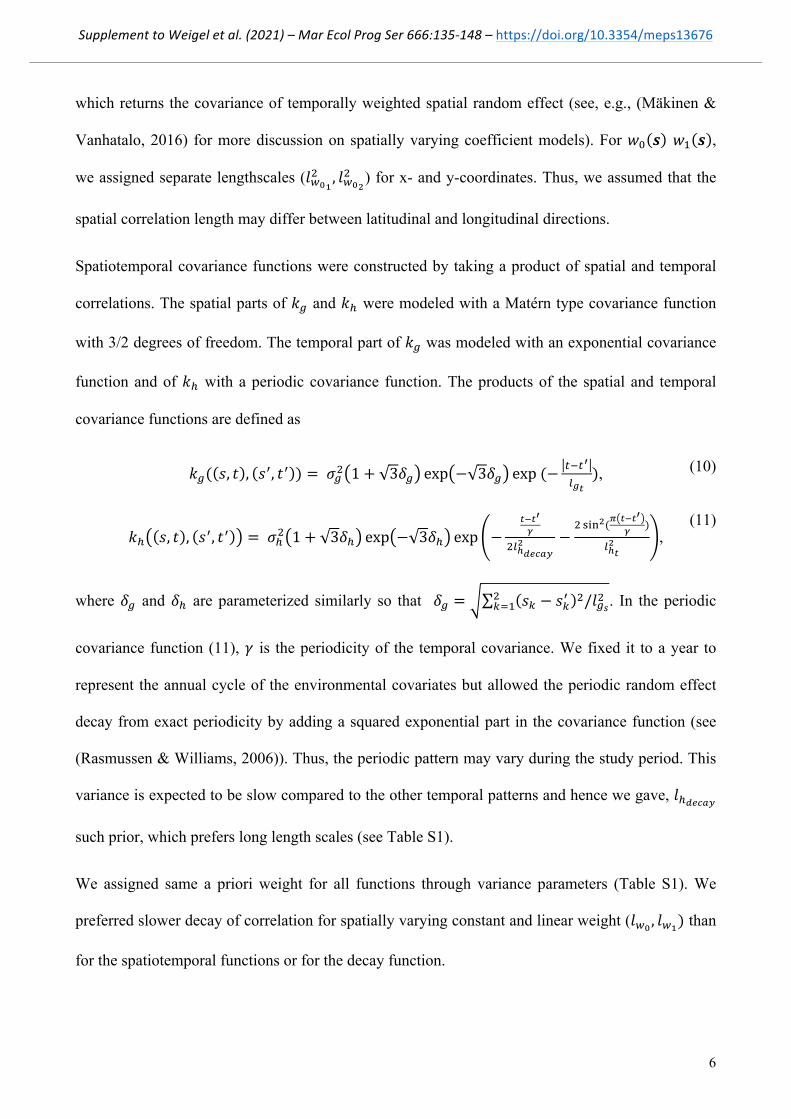
Estimates for the model parameters, magnitudes of variation and lengthscales, differ between

covariates, which shows that the covariates follow different spatio-temporal patterns (see Table S2).

We checked how big proportion of the variation in the observations of the covariates was explained

by each model component (see Table S2). Most of the variation was explained with random effects

and only a small proportion was explained with a random residual error. Temperature and

chlorophyll α were most explained by the periodic spatio-temporal random effect, whereas salinity

was most explained with the spatial random effect. Chlorophyll α was explained to a remarkable

extent also with the non-periodic spatio-temporal random effect. The parameters governing the

spatial correlation length of the most important function for each covariate were estimated relatively

low (temperature: 87.69 km; salinity: 9.01 km and 6.81 km; chlorophyll α 7.15 km) compared to the

estimates of spatial correlation lengths of other functions.


8

The decay in the periodic spatio-temporal random effect was relatively long for temperature (239

years) and chlorophyll α (62 years), and clearly shorter for salinity and (36 years) (see Table S2).

For the two latter the decay of the periodic spatio-temporal random effect is less influential since

the random effect explains clearly less than the solely spatial random effect.

Table S2. Estimates of the parameter values for each covariate.

Parameter Temperature Salinity Chlorophyll α !!!! 0.03 0.58 0.26 !!!! 0.06 0.07 0.04 !!! 0.11 0.09 0.36 !!! 1.59 0.15 0.66 !!! 0.03 0.05 0.11 !!!! 2.81 9.01 138.42 !!!! 237.29 6.81 274.90 !!!! 364.52 377.70 551.56 !!!! 508.40 318.07 521.32 !!! 0.02 0.12 0.04 !!! 231.31 10.11 5.03 !!! 1.33 1.07 0.56 !! 238.64 35.58 61.78 !!! 87.69 8.89 7.15

Comparison and validation

We built two different models regarding the random effects and made a model comparison by

computing their log predictive posterior densities (LPPD) (Vehtari, Gelman, & Gabry, 2016)

!""# = !"# ! !! !! , !! ,! ! !|!,!, ! !" !!!! . (9)

Here we computed the model fit by integrating the probabilities of unseen observations over the

posterior of unknown hyperparameters and summing the log probabilities of all unseen points. We

decrease the dependence of training and validation data sets by using leave-one-out cross-validation

(LOO-CV). One by one, each data point is left out from training data set and used as a validation


9

data point. We chose the model structure presented here due to it resulting with higher LPPD than

the other model candidates.

To validate the use of the predictions from the spatio-temporal models, we applied spatially and

temporally explicit cross-validation methods. In both cross-validation schemes, we picked 25

evaluation observations, which we evaluated one by one. We created a spatial or temporal buffer

around the evaluation point and discarded all observations from inside the buffer. Lastly, we

predicted the covariate value in the evaluation point given all other data points, as in (Le Rest,

Pinaud, Monestiez, Chadoeuf, & Bretagnolle, 2014). We did not infer the hyperparameter values

after discarding the points under the buffer zone. We argue that this was a reasonable choice since

we inferred the parameter values with an even smaller data set than the data that we used for

creating covariate predictions in study areas, and the interest is not in deriving specifically accurate

hyperparameter estimates but in predicting accurately the covariate values.

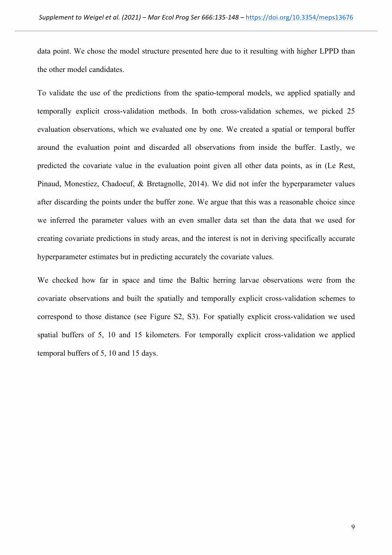
We checked how far in space and time the Baltic herring larvae observations were from the

covariate observations and built the spatially and temporally explicit cross-validation schemes to

correspond to those distance (see Figure S2, S3). For spatially explicit cross-validation we used

spatial buffers of 5, 10 and 15 kilometers. For temporally explicit cross-validation we applied

temporal buffers of 5, 10 and 15 days.


10

Figure S3. Spatio-temporal distance of study areas from the closest environmental covariate

observations.

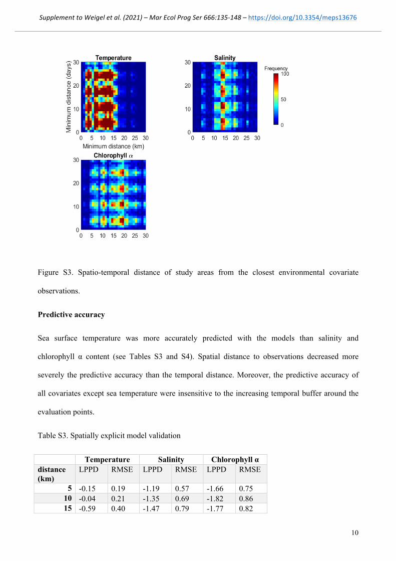
Predictive accuracy

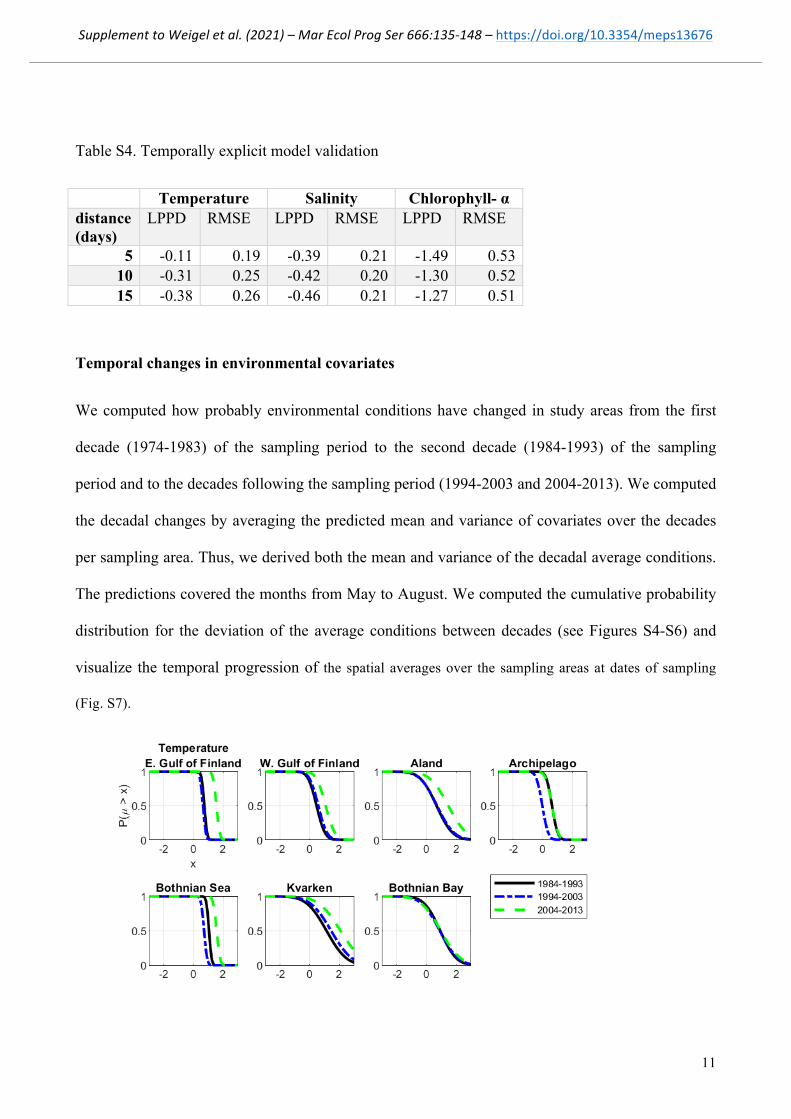
Sea surface temperature was more accurately predicted with the models than salinity and

chlorophyll α content (see Tables S3 and S4). Spatial distance to observations decreased more

severely the predictive accuracy than the temporal distance. Moreover, the predictive accuracy of

all covariates except sea temperature were insensitive to the increasing temporal buffer around the

evaluation points.

Table S3. Spatially explicit model validation

Temperature Salinity Chlorophyll α distance (km)

LPPD RMSE LPPD RMSE LPPD RMSE

5 -0.15 0.19 -1.19 0.57 -1.66 0.75 10 -0.04 0.21 -1.35 0.69 -1.82 0.86 15 -0.59 0.40 -1.47 0.79 -1.77 0.82


11

Table S4. Temporally explicit model validation

Temperature Salinity Chlorophyll- α distance (days)

LPPD RMSE LPPD RMSE LPPD RMSE

5 -0.11 0.19 -0.39 0.21 -1.49 0.53 10 -0.31 0.25 -0.42 0.20 -1.30 0.52 15 -0.38 0.26 -0.46 0.21 -1.27 0.51

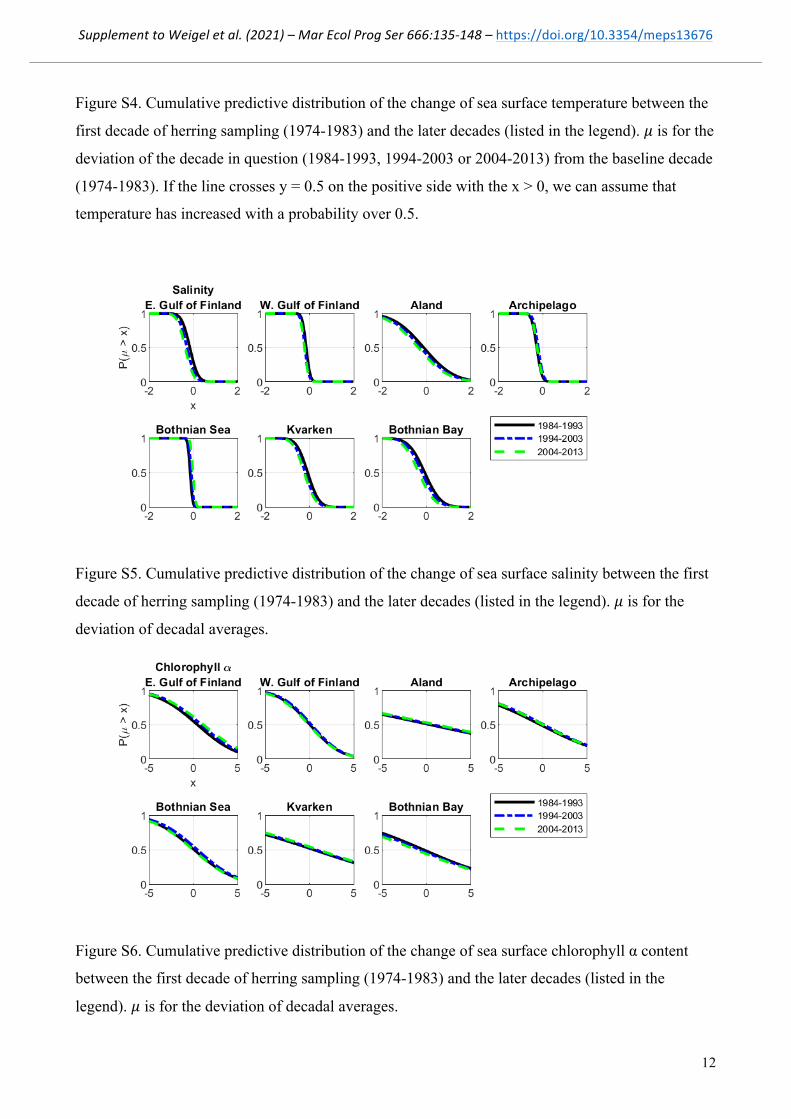
Temporal changes in environmental covariates

We computed how probably environmental conditions have changed in study areas from the first

decade (1974-1983) of the sampling period to the second decade (1984-1993) of the sampling

period and to the decades following the sampling period (1994-2003 and 2004-2013). We computed

the decadal changes by averaging the predicted mean and variance of covariates over the decades

per sampling area. Thus, we derived both the mean and variance of the decadal average conditions.

The predictions covered the months from May to August. We computed the cumulative probability

distribution for the deviation of the average conditions between decades (see Figures S4-S6) and

visualize the temporal progression of the spatial averages over the sampling areas at dates of sampling

(Fig. S7).


12

Figure S4. Cumulative predictive distribution of the change of sea surface temperature between the

first decade of herring sampling (1974-1983) and the later decades (listed in the legend). ! is for the

deviation of the decade in question (1984-1993, 1994-2003 or 2004-2013) from the baseline decade

(1974-1983). If the line crosses y = 0.5 on the positive side with the x > 0, we can assume that

temperature has increased with a probability over 0.5.

Figure S5. Cumulative predictive distribution of the change of sea surface salinity between the first

decade of herring sampling (1974-1983) and the later decades (listed in the legend). ! is for the

deviation of decadal averages.

Figure S6. Cumulative predictive distribution of the change of sea surface chlorophyll α content

between the first decade of herring sampling (1974-1983) and the later decades (listed in the

legend). ! is for the deviation of decadal averages.


13

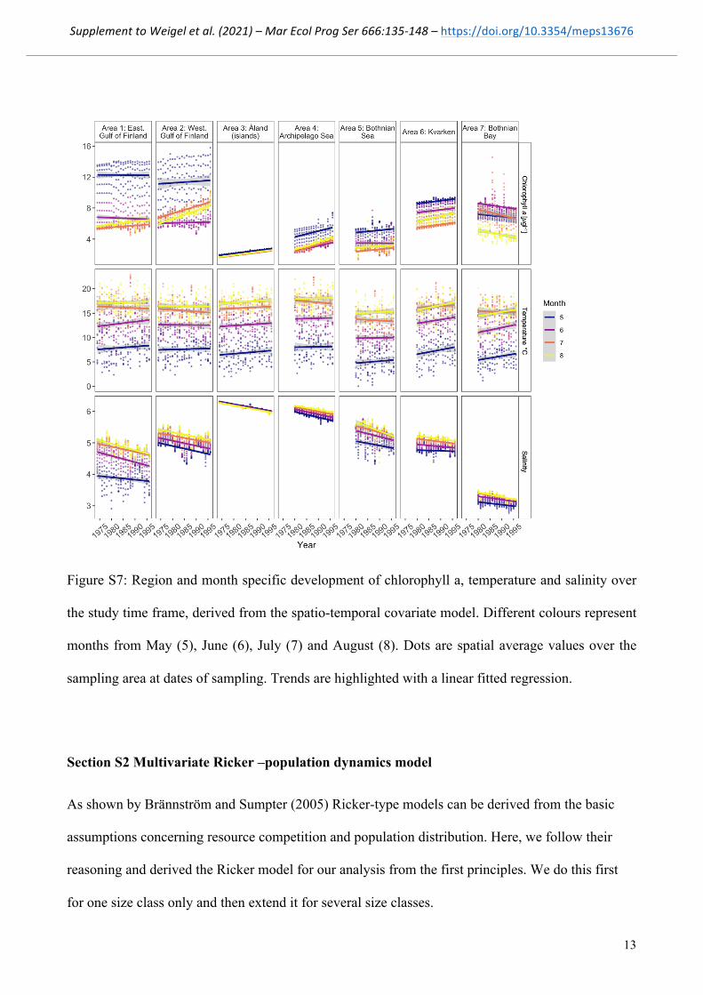
Figure S7: Region and month specific development of chlorophyll a, temperature and salinity over

the study time frame, derived from the spatio-temporal covariate model. Different colours represent

months from May (5), June (6), July (7) and August (8). Dots are spatial average values over the

sampling area at dates of sampling. Trends are highlighted with a linear fitted regression.

Section S2 Multivariate Ricker –population dynamics model

As shown by Brännström and Sumpter (2005) Ricker-type models can be derived from the basic

assumptions concerning resource competition and population distribution. Here, we follow their

reasoning and derived the Ricker model for our analysis from the first principles. We do this first

for one size class only and then extend it for several size classes.


14

We denote by !!,! the spawning stock size in stock assessment region ! (see Fig. 1 in the main text)

at year !. Further, we denote by !!,!,! = !!,!!!,! the spawning stock size in area ! inside stock

assessment region !. The parameter !!,! corresponds to the proportion of the total spawning stock

that spawns in area ! and for simplicity we assume it to be time independent here. We then assume

that the reproductive success of each spawning individual is ! !, ! = !(!)!! where ! is the

number of other individuals within an area ! centered on the focal individual. The reproductive

success is a parameter describing the expected number of larvae produced by a spawner that survive

to a given larval size class. The parameter ! ! > 0 is a function of environmental covariates !

which describes the rate of reproduction of spawners and the larvae growth and competition

independent survival until the size class. The parameter 1− ! ∈ (0,1) is the intensity of

competition; that is the smaller ! is the larger the competition between individuals is and, hence, the

more rapidly the reproductive success of an individual decreases as the number of other individuals

increases within the neighborhood around it. Thus, the expected number of larvae produced in area

! is

! !!,!,! = !!,!!!,! !!,!(!)!!,!!!,!!!! ! !, ! (10)

where !!,!(!) is the probability of an individual in area ! having exactly ! neighbors within area !.

Given that !!,! is small compared to !!,!, and assuming that the individuals in area ! are randomly

distributed within the area, the probability distribution for the number of neighbors ! can be

accurately approximated with a Poisson distribution with expectation !!,!,!!/!!,! where !!,! is the

size (area) of sampling area !. Hence,

! !!,!,!!!,!

|!!,! , ! = !!,!! ! !!!!,!,!!/!!,!!!!,!,!!/!!,!

!

!!!!!! = !!,!! ! !

!!(!!!)!!,!!!,!!!,! (11)


15

which is of the same form as the Ricker model (Ricker 1954). Next, we add stochasticity to the

model by adding i.i.d. Gaussian random effect, !!,!, to the exponential and simplify the notation by

denoting

!!,! = − !!,!! !!!!!,!

, !!,! = log!!,! and ! ! = log ! ! (12)

so that the logarithm of number of larvae per SSB, to be called larval production rate, can be written

as

log !!,!,!!!,!

|!!,! , ! = !! + ! ! + !!,!!!,! + !!,! . (13)

This is a standard linear regression model where !! is an area-specific intercept corresponding to

log proportion of spawning stock biomass in area !, ! ! is a function describing the effect of

environment to the rate of reproduction and survival of larvae and !!,! < 0 is an area-specific

regression coefficient corresponding to the density dependent decrease in reproduction success of

an individual (up until a given larval size class). Since we have data on both larval and spawning

stock biomass, equation (13) means that we can implement the Ricker model with any linear or

additive mixed effects model to recover the effects of environment and density dependence to the

larval production rate. We just need to first specify the regression function ! ! . However, since

the covariates, larval and spawning stock biomass data contain noise, the residual terms !!,! explain

both process stochasticity and residual error due to noisy data.

Equation (13) can be easily extended for larvae of different size classes. Let’s denote by !!,!,!,!, the

number of larvae in size class, !, and write the Ricker model as

log !!,!,!,!!!,!

|!!,! , ! = !!,! + !! ! + !!,!,!!!,! + !!,!,! . (14)

where the parameters !!,!, !!,!,! and regression function !! ! are size class specific. The

interpretation of these size class specific parameters is the same as in the one size class case but


16

now the model allows different environmental and density dependent processes for different size

classes. For example, if !!,!,! was close to zero for smallest size classes and negative for larger size

classes, there would be density dependent competition only between larger larvae.

References

Banerjee, S., Gelfand, A. E., & Carlin, B. P. (2015). Hierarchical modeling and analysis for spatial

data (second ed.). Boca Raton. CRC Press.

Brännström, Å. and Sumpter, D. J. T. 2005. The role of competition and clustering in

population dynamics. - Proc. R. Soc. B Biol. Sci. 272: 2065–2072

Le Rest, K., Pinaud, D., Monestiez, P., Chadoeuf, J., & Bretagnolle, V. (2014). Spatial leave-‐one-‐

out cross-‐validation for variable selection in the presence of spatial autocorrelation. Global

Ecology and Biogeography, 23, 811-820.

Mäkinen, J., & Vanhatalo, J. (2016). Hydrographic responses to regional covariates across the Kara

Sea. Journal of Geophysical Research: Oceans, 121, 8872-8887.

Parmanne, R. 2001. Abundance of Baltic herring larvae off the coast of Finland in 1974-1996.

Kalatutkimuksia - Fiskundersökningar (in Finnish with English summary). 170.

Rasmussen, C. E., & Williams, C. K. I. (2006). Gaussian processes for machine learning. MIT

Press.

Ricker, W. E. 1954. Stock and Recruitment. - J. Fish. Res. Board Canada 11: 559–623.

Vehtari, A., Gelman, A., & Gabry, J. (2016). Practical Bayesian model evaluation using leave-one-

out cross-validation and WAIC. Statistics and Computing, 27, 1413-1432.

Wikle, C. K. (2003). Hierarchical Models in Environmental Science. International Statistical

Review, 71, 181-199.

m 13676 supplement 1 use - int-res.com

Documents