low-cost navigation systems a study of four …280511/fulltext01.pdflow-cost navigation systems a...
TRANSCRIPT

Low-Cost Navigation SystemsA Study of Four Problems
ISAAC SKOG
Doctoral Thesis in Signal Processing
Stockholm, Sweden 2009

TRITA-EE 2009:057ISSN 1653-5146ISBN 978-91-7415-528-0
KTH, School of Electrical EngineeringACCESS Linnaeus Center
Signal Processing LaboratorySE-100 44 Stockholm
SWEDEN
Akademisk avhandling som med tillstånd av Kungl Tekniska högskolanframlägges till offentlig granskning för avläggande av teknologie doktorsex-amen i signalbehandling fredagen den 22 jan 2010 klockan 10.00 i hörsalF3, Lindstedtsvägen 26, Stockholm.
© Isaac Skog, December 2009
Tryck: Universitetsservice US AB

iii
For the pleasure of finding things out!

Abstract
Today the area of high-cost and high-performance navigation for vehiclesis a well-developed field. The challenge now is to develop high-performancenavigation systems using low-cost sensor technology. This development in-volves problems spanning from signal processing of the dirty measurementsproduced by low-cost sensors via fusion and synchronization of informationproduced by a large set of diverse sensors, to reducing the size and energyconsumption of the systems. This thesis examines and proposes solutionsto four of these problems.
The first problem examined is the time synchronizing of the sensor datain a global positioning system aided inertial navigation system in which nohardware clock synchronization is possible. A poor time synchronizationresults in an increased mean square error of the navigation solution andexpressions for calculating this mean square error are presented. A methodto solve the time synchronization issue in the data integration software isproposed. The potential of the method is illustrated with tests on real-world data that are subjected to timing errors.
The second problem examined is the achievable clock synchronizationaccuracy in a sensor network employing a two-way message exchange model.The Cramér-Rao bound for the estimation of the clock parameters is de-rived and transformed into a lower bound on the mean square error of theclock offset. Further, an approximate maximum likelihood estimator forthe clock parameters is proposed. The estimator is shown to be of lowcomplexity and to have a mean square error in the vicinity of the Cramér-Rao bound.
The third problem examined is the detection of the time epochs whenzero-velocity updates can be applied in a foot-mounted pedestrian navi-gation system. Four general likelihood ratio tests for detecting when thenavigation system is stationary based on the inertial measurement data arestudied. The performance of the four detectors is evaluated using levelledground, forward-gait data. The results show that the signals from the gy-roscopes hold the most reliable information for the zero-velocity detection.
The fourth problem examined is the calibration of a low-cost inertialmeasurement unit. A calibration procedure that relaxes the accuracy re-
v

vi ABSTRACT
quirements of the orientation angles the inertial measurement unit mustbe placed in during the calibration is studied. The proposed calibrationmethod is compared with the Cramér-Rao bound for the case when theinertial measurement unit is rotated into precisely controlled orientations.Simulation results show that the mean square error of the estimated sen-sor model parameters reaches the Cramér-Rao bound within few decibels.Thus, the proposed method may be acceptable for a wide range of low-costapplications.

Acknowledgements
Five years of work on my thesis are coming to an end, and I would liketo take this opportunity to express my gratitude to all those who havesupported me.
First and foremost, I would like to thank my supervisor, Professor PeterHändel, who, for five years, has shared his knowledge in a most inspiringway. Thank you for your guidance and support. This journey has beena pure pleasure! Professor Magnus Jansson, thank you for being my co-supervisor. You have given me many valuable inputs and ideas. AndProfessor Mats Bengtsson, thank you for all your help in solving Latexproblems.
To my present and former fellow doctoral students and all my colleaugesat the Signal Processing Lab, thank you for the interesting and stimulatingdiscussions and for all the fun during the social events. I would also liketo thank Annika Augustsson for taking care of a variety of administrativeissues and for creating an enjoyable work environment: You spoil us!
I would also like to thank Professor Naser El-Sheimy and the rest of theMobile Multi-Sensor System Research group at the University of Calgaryfor the opportunity to be a part of your research team for six months. Ilearned a great deal.
I am grateful to Professor Fredrik Gustafsson for acting as the opponentto this thesis, and Professor Danica Kragic, Professor Karl-Johan Åström,and Peter Hessling for participating in the grading committee.
Last but not the least, I would like to express my heartfelt thanks tomy family and all my friends for supporting me. You bring joy to my life.
Isaac SkogStockholm, December 2009
vii
Contents
Abstract v
Acknowledgements vii
Contents viii
1 Low-Cost Navigation Systems 11.1 Navigation . . . . . . . . . . . . . . . . . . . . . . . . . . . . 11.2 Problems in Low-Cost Navigation Systems . . . . . . . . . . 11.3 Thesis Outline and Contributes . . . . . . . . . . . . . . . . 31.4 Related Research . . . . . . . . . . . . . . . . . . . . . . . . 61.5 Further Research . . . . . . . . . . . . . . . . . . . . . . . . 7
2 In-Car Navigation Technologies 92.1 Introduction . . . . . . . . . . . . . . . . . . . . . . . . . . . 92.2 State of the Art Systems . . . . . . . . . . . . . . . . . . . . 112.3 GNSS and Augmentation Systems . . . . . . . . . . . . . . 132.4 Motion Sensors and Coordinate Systems . . . . . . . . . . . 192.5 Information Processing . . . . . . . . . . . . . . . . . . . . . 252.6 Map Information . . . . . . . . . . . . . . . . . . . . . . . . 302.7 Information Fusion . . . . . . . . . . . . . . . . . . . . . . . 332.8 Conclusions . . . . . . . . . . . . . . . . . . . . . . . . . . . 39
3 Time Synchronization in GPS-aided INS 433.1 Introduction . . . . . . . . . . . . . . . . . . . . . . . . . . . 433.2 MSE of the State Estimate . . . . . . . . . . . . . . . . . . 453.3 Estimating and Removing the Timing Error . . . . . . . . . 553.4 Time Synchronization in GPS-aided INS . . . . . . . . . . . 603.5 Observability Analysis . . . . . . . . . . . . . . . . . . . . . 673.6 Conclusions . . . . . . . . . . . . . . . . . . . . . . . . . . . 713.A Extended State Space Model Error Covariance . . . . . . . 733.B INS Error Model . . . . . . . . . . . . . . . . . . . . . . . . 743.C Observability Matrices . . . . . . . . . . . . . . . . . . . . . 76
viii

Contents ix
4 Synchronization by Message Exchanges 774.1 Introduction . . . . . . . . . . . . . . . . . . . . . . . . . . . 774.2 Problem Description . . . . . . . . . . . . . . . . . . . . . . 794.3 The Two-Way Message Exchange Model . . . . . . . . . . . 814.4 Cramér-Rao Bound . . . . . . . . . . . . . . . . . . . . . . . 844.5 Approximative Maximum Likelihood Estimator . . . . . . . 934.6 Simulation Study . . . . . . . . . . . . . . . . . . . . . . . . 974.7 Conclusions . . . . . . . . . . . . . . . . . . . . . . . . . . . 1014.A FIM Elements . . . . . . . . . . . . . . . . . . . . . . . . . . 1034.B Polynomial Functions in the CRB Expressions . . . . . . . 1034.C Proofs of the Inequalities . . . . . . . . . . . . . . . . . . . 104
5 Zero-Velocity Detection 1075.1 Introduction . . . . . . . . . . . . . . . . . . . . . . . . . . . 1075.2 Problem Definition . . . . . . . . . . . . . . . . . . . . . . . 1085.3 Signal and Sensor Model . . . . . . . . . . . . . . . . . . . . 1105.4 Generalized Likelihood Ratio Test . . . . . . . . . . . . . . 1125.5 Performance Evaluation . . . . . . . . . . . . . . . . . . . . 1195.6 Conclusions . . . . . . . . . . . . . . . . . . . . . . . . . . . 124
6 Calibration of a MEMS IMU 1276.1 Introduction . . . . . . . . . . . . . . . . . . . . . . . . . . . 1276.2 Sensor Error Model . . . . . . . . . . . . . . . . . . . . . . . 1296.3 Calibration Algorithm . . . . . . . . . . . . . . . . . . . . . 1326.4 Cramér-Rao Bound . . . . . . . . . . . . . . . . . . . . . . . 1346.5 Results . . . . . . . . . . . . . . . . . . . . . . . . . . . . . . 1366.6 Conclusions . . . . . . . . . . . . . . . . . . . . . . . . . . . 1396.A FIM Elements . . . . . . . . . . . . . . . . . . . . . . . . . . 141
Bibliography 143

Chapter 1
Low-Cost Navigation Systems
1.1 Navigation
”Navigation – the science of getting ships, aircraft, or spacecraft from placeto place; especially the method of determining position, course, and distancetravelled.” [Mer09].
This is the definition of the word navigation given in [Mer09]. Withinthis thesis the words navigation, and navigation system, are used withrespect to the latter part, (i.e., the method of determining position andcourse, and the system performing this task). The thesis will investi-gate four problems encountered in the development of low-cost vehicle andpedestrian navigation systems, and propose possible solutions.
1.2 Problems in Low-Cost Navigation Systems
Today the area of high-cost and high-performance navigation for ground,sea, underwater, or air vehicles is a well developed field. The challenge nowis to develop high-performance navigation systems using low-cost sensortechnology or pedestrian indoor navigation systems. This development in-volves problems spanning from signal processing of the dirty measurementsproduced by low-cost sensors via fusion and synchronization of informationproduced by a large set of diverse sensors, to reducing the size and energyconsumption of the systems.
To get a picture of the problems encounter going from high to low-costnavigation, the navigation problem may be studied with start from theinformation classes available and the quality of the sensors employed toextract the information. With reference to Figure 1.1, looking at the nav-igation problem from an information perspective, there are basically fourdifferent classes of information sources available: (1) active external in-frastructure sources such as various global navigation satellite systems and
1

2 CHAPTER 1. LOW-COST NAVIGATION SYSTEMS
Active External Sources Passive External Sources
Self Contained Motion Sensors Motion Constraints
Information
Fusion
Figure 1.1: The four basic classes of navigation information.
other radio frequency based navigation systems; (2) passive external infras-tructure sources such as land marks or radio-frequency identification tagsthat may be read by onboard sensors; (3) self-contained motion sensorslocated onboard the navigation platform, such as accelerometers, veloc-ity encoders, and gyroscopes; (4) motion constraints information sourcessuch as road or building maps, and vehicle or human motion models. Thedesigner of a navigation system must choose which of these types of infor-mation sources, if not all, to use, and how to combine them to meet theperformance requirements. This necessitates a balance between the cost,complexity, and performance of the system.
In the design of a high-cost vehicle navigation system the designer mayget away by relying on a few high quality sensors extracting informationfrom one or two of the information sources. However, in the design ofa low-cost vehicle navigation system, the information quality provided bycheaper sensors, may force the designer to work with a large variety ofsensors, employing information from all of the four information classes, tofulfill the performance requirements. This means that complexity of thesystem increases, since:
• The information fusion filter must be able to manage many differentinformation sources with varying characteristics.
• The information from many sources, possibly widely separated withinthe system must be communicated, synchronized, and spatially re-lated.
• The dirty sensor measurements must be compensated for by usingrefined error models, calibration schemes and motion models.

1.3. THESIS OUTLINE AND CONTRIBUTES 3
Designing a robust pedestrian navigation system, especially to provideseamless navigation in indoor and harsh radio environments without prein-stalled dedicated infrastructure, is an even more challenging problem. Theadditional complexity is owing to several facts. In an indoor or in a harshradio environment the backbone of most of today navigation systems, theglobal positioning system, works poorly. The complex motion of the hu-man body in comparison to the ridge chassis of a vehicle makes it hard toconstruct motion models, and spatially relate measurements from sensorslocated on different body parts. Finally, the size and power consumptionof the systems must be further reduced. A more in-depth introduction anddescription of the problems encountered in the development of low-costnavigation systems is presented in Chapter 2.
1.3 Thesis Outline and Contributes
The outline of the thesis is as follows. Chapter 2, presents a survey onin-car navigation and serves as an introduction to the remaining chaptersby describing the major navigation information sources, their characteris-tics, and common methods used to combine them. Chapters 3–6 are thendevoted to detailed investigations of four problems related to the devel-opment of low-cost vehicle and pedestrian navigation systems. The fourproblems treated are the time synchronization in a global positioning sys-tem aided inertial navigation system, the time synchronization of wirelesssensor nodes by two-way message exchanges, the zero-velocity detection ina foot-mounted pedestrian navigation system, and the calibration of iner-tial measurement unit. A summary of each chapter is given next.
Chapter 2
This chapter presents a survey of the information sources and informationfusion technologies used in current in-car navigation systems. The naviga-tion system performance measurements of accuracy, integrity, availability,and continuity of service, are introduced. General principles of operationand, pros and cons of the four commonly used information sources – re-ceivers for radio based positioning using satellites, vehicle motion sensors,vehicle models, and digital map information – are described. Common fil-ters and system architectures to combine the information from the varioussources are discussed. The chapter is based upon:
• I. Skog and P. Händel. In-Car Positioning and Navigation Technolo-gies – A Survey. IEEE Trans. on Intelligent Transportation Systems,10(1):4-21, March 2009.
4 CHAPTER 1. LOW-COST NAVIGATION SYSTEMS
Chapter 3
This chapter presents a study of the effects of a time synchronization er-ror in a loosely coupled global positioning system aided inertial navigationsystem. It is shown that a time synchronization error increases the meansquare error of the estimated navigation solution. Expressions for evalu-ating the mean square error of the navigation solution, given the vehicletrajectory and the model of the inertial navigation system error dynamics,are derived. Two different cases are studied in some detail. The first caseconsiders a navigation system in which the timing error is not includedin the integration filter. This leads to a system with an increased meansquare error and a bias in the estimated forward acceleration. In the sec-ond case, a parametrization of the timing error is included as a part of theestimation problem in the data integration. The estimated timing erroris fed back to control an adjustable fractional delay filter, synchronizingthe inertial measurement unit and the global positioning system receiverdata. Simulation results show that by including the timing error in the es-timation problem, almost perfect time synchronization is obtained and thebias in the forward acceleration is removed. The potential of the proposedmethod is illustrated with tests on real-world data that are subjected totiming errors. Moreover, through an observability analysis, it is shown thatthe timing error is observable for all trajectories that include accelerationchanges. The chapter is based upon:
• I. Skog and P. Händel, Time synchronization errors in GPS-aided in-ertial navigation systems. IEEE Trans. on Intelligent TransportationSystems, In revision, 2009.
A shorter version is available as:
• I. Skog and P. Händel, Effects of time synchronization errors in GNSS-aided INS. In Proc. of PLANS 2008, Monterey, CA, USA, April 2008.
The material on the observability analysis is excluded from the precedinglisted publications, and is under consideration for a future publication.
Chapter 4
This chapter presents a study of the achievable clock synchronization accu-racy in a wireless sensor network employing a two-way message exchangemodel. The Cramér-Rao bound for the estimation of the clock parame-ters is derived for four different parameterizations (i.e., different nuisanceparameters), reflecting different levels of prior knowledge concerning thesystem parameters. The results on the Cramér-Rao bound are transformedinto a lower bound on the mean square error of the clock offset, a figure of

1.3. THESIS OUTLINE AND CONTRIBUTES 5
merit often more relevant, characterizing the system performance. Further,by introducing a set of artificial observations through a linear combinationof the observations originally obtained in the two-way message exchange,an approximate maximum likelihood estimator for the clock parameters isproposed. The estimator is shown to be of low complexity and it obeysnear-optimal performance, that is, a mean square error in the vicinity ofthe Cramér-Rao bound. The applicability of the derived results is shownthrough a simulation study of an offshore engineering scenario, where aremotely operated underwater vehicle is used for operations at the seabed.The position of the vehicle is tracked using a wireless sensor network. Thechapter is based upon:
• I. Skog and P. Händel. Synchronization by Two-Way Message Ex-changes: Cramér-Rao Bounds, Approximate Maximum Likelihood,and Offshore Submarine Positioning. IEEE Trans. on Signal Pro-cessing, Accepted for publication with mandatory minor revisions,May 2009.
Chapter 5
This chapter presents a study of the problem of detecting the time epochswhen zero-velocity updates can be applied in a foot mounted pedestriannavigation system. Three, in the literature, commonly used detectors areexamined: the acceleration moving variance detector, the acceleration mag-nitude detector, and the angular rate energy detector. It is shown that alldetectors can be derived within the same general likelihood ratio test frame-work – given different prior knowledge about the sensor signals. Further,by combining all prior knowledge, a new likelihood ratio test detector isderived. The performance of the detectors is then evaluated using slow(approx. 3 km/h) and fast (approx. 5 km/h), levelled ground, forward-gait data. As a reference system, indicating when the inertial measurementunit is stationary, force sensitive resistors mounted beneath the foot of theuser are used. The test results are presented in terms of the detectionversus false alarm probability. The results show that the new detector per-forms marginally better than the angular rate energy detector, which outperforms both the acceleration moving variance detector and accelerationmagnitude detector. The conclusion is therefore that, under the conditionsstated, the signals from the gyroscope assembly hold the most reliable in-formation for zero-velocity detection. The chapter is based upon:
• I. Skog and P. Händel. Zero-Velocity Detection in Pedestrian Naviga-tion Systems – An Algorithm Evaluation. IEEE Trans. on Biomedi-cal Engineering, Submitted, Nov. 2009.

6 CHAPTER 1. LOW-COST NAVIGATION SYSTEMS
Chapter 6
This chapter presents an approach for calibrating a low-cost inertial mea-surement unit, requiring no mechanical platform for the accelerometer cal-ibration and only a simple rotating table for the gyro calibration. Theproposed calibration methods utilize the fact that ideally the norm of themeasured output of the accelerometer and gyro cluster is equal to the mag-nitude of applied force and rotational velocity, respectively. This fact,together with a model of the sensors is used to construct a cost function,which is minimized with respect to the unknown model parameters usingNewton’s method. The performance of the calibration algorithm is com-pared with the Cramér-Rao bound for the case when a mechanical platformis used to rotate the inertial measurement unit into different precisely con-trolled orientations. Simulation results shows that the mean square errorof the estimated sensor model parameters reaches the Cramér-Rao boundwithin 8 dB, and thus the proposed method may be acceptable for a widerange of low-cost applications. The chapter is based upon:
• I. Skog and P. Händel. Calibration of a MEMS Inertial MeasurementUnit. In Proc. of IMEKO 2006, Rio de Janeiro, Brazil, September2006.
Note that there is no cross-referencing between the chapters in the thesis;instead, references are made to the preceding listed published material.Further, the mathematical notation employed in the thesis is adapted tothe problem under investigation and thus varies between the chapters. Thenotation employed is defined within each chapter.
1.4 Related Research
Results from three other research projects in the field of vehicle and pedes-trian navigation, which I have been involved in, have been omitted fromthe thesis. The first of these projects was concerned with the developmentof a test and demonstrator platform for low-cost global positioning systemaided inertial navigation. The results of the project are presented in:
• I. Skog and P. Händel. A low-cost GPS aided inertial navigationsystem for vehicle applications. In Proc. of EUSIPC 2005, Antalaya,Turkey, September 2005.
• I. Skog and A. Schumacher and P. Händel. A Versatile PC-BasedPlatform for Inertial Navigation. In Proc. of NORSIG 2006, Reyk-javik, Iceland, June 2006.
The second project investigates existing techniques for positioning of emer-gency personal. The results of the project are presented in:
1.5. FURTHER RESEARCH 7
• J. Rantakokko, P. Händel, F. Eklöf, B. Boberg, M. Junered, D. Akos,I. Skog, H. Bohlin, F. Neregård, F. Hoffmann, D. Andersson, M. Jans-son, and P. Stenumgaard. Positioning of emergency personnel in res-cue operations - possibilities and vulnerabilities with existing tech-niques and identification of needs for future R&D. Technical reportTRITA-EE 2007:037, Royal Institute of Technology, 2007, Stock-holm, Sweden.
• J. Rantakokko, J. Rydell, K. Fors, S. Linder, S. L. Wirkander, I. Skog,and P. Händel. Technologies for first responder indoor localization. InPrecision Indoor Personnel Location and Tracking for Emergency Re-sponders Technology Workshop, Worcester, MA, USA, August 2009.
The third project is on the development, construction, and test of an ultrawide band radio aided inertial navigation system for indoor positioning.Initial results are found in:
• J. O. Nilsson, A. De Angelis, I. Skog, P. Carbone, and P. Händel.Signal processing issues in indoor positioning by ultra wide bandradio aided inertial navigation. In Proc. of EUSIPCO 2009, Glasgow,Scotland, September 2009.
• A. De Angelis, J. O. Nilsson, I. Skog, P. Händel, and P. Carbone.Indoor Positioning by Ultra Wide Band Radio Aided Inertial Navi-gation. In Proc. of IMEKO 2009, Lisbon, Portugal, September 2009.
Another research project, not in the field of navigation but in the closelyrelated field of advanced driver assistant systems, in which I have beeninvolved, is the moose early warning system project. The project evaluatedthe feasibility of using an off-the-shelf consumer electronics infrared camerato construct a system that at an early stage warns the driver when thereis a moose on or close to the road. The results of the project are presentedin:
• P. Händel, Y. Yao, N. Unkuri, and I. Skog. Far infrared cameraplatform and experiments for moose early warning systems. JSAETrans., 40(4):1095–1099, July 2009.
1.5 Further Research
During the research that bred to the results presented in the thesis, severalquestions and research ideas have emerged. A selection of these is outlinednext.
8 CHAPTER 1. LOW-COST NAVIGATION SYSTEMS
Time Synchronization
In Chapter 3, a method to estimate and compensate for a constant timesynchronization error in the data sampling in a loosely coupled global po-sitioning system aided inertial navigation system is proposed. A naturaldevelopment of this work is to investigate the possibility of extending themethod to work with a tightly coupled system architecture and a time-varying synchronization error. Moreover, it would be interesting to developa framework for time synchronization in sensor networks consisting of a setof slave nodes that can transmit but not receive data, and one master noderesponsible for the data fusion. This could possibly be completed by com-bining the clock skew estimation method in Chapter 4, and the constanttime synchronization error (i.e., the initial clock offset) estimation methodin Chapter 3.
Zero-Velocity Detection for Pedestrian Navigation
In Chapter 5, the detection versus false alarm probability performance offour zero-velocity detectors for pedestrian navigation systems is evaluated.An extension of this work would be to investigate how these performancefigures relates to the accuracy of the of the navigation solution in a pedes-trian navigation system employing the different detectors.
Inertial Measurement Unit Calibration
In Chapter 6, a calibration method that simplifies the inertial sensor cali-bration by not requiring the inertial measurement unit to be rotated intoprecisely controlled orientations, is studied. The accuracy of the calibrationmethod is compared to the Cramér-Rao bound for the calibration methodwhere the inertial measurement unit is rotated into precisely controlledorientations. The calibration method has later been refined and furtherevaluated in [FON08]. To better access the theoretical achievable accuracyof the calibration method a tighter bound could be calculated by treatingthe unknown orientations as nuisance parameters in the derivation of theCramér-Rao bound.
Chapter 2
In-Car Navigation Technologies
2.1 Introduction
Today a large share of passenger cars is delivered from the factory with aGPS-based in-car navigation system. Owners of used cars can at, a rea-sonable cost, install one of the many third party in-car navigation systemson the market. Indeed, in Western Europe around 14.4 million portablesatellite navigation systems were sold during 2007 [GfK08]. These nav-igation aids are designed to support the driver by showing the vehicle’scurrent location on a map and by giving both visual and audio informationon how to efficiently get from one location to another, i.e., route guid-ance. Moreover, many vehicles used in professional services, such as taxis,buses, ambulances, police cars and fire trucks, are today equipped withnavigation systems that not only show the current location but also con-stantly communicate the vehicle location to a monitoring center. Oper-ators at the center can use this information to direct the vehicle feet aseffciently as possible. To further improve the usefulness of these in-carnavigation systems, for example, with information such as when, whereand how to make lane changes with respect to the planned course changes,the accuracy of both the navigation systems and digital maps has to beimproved [DB06, DB04, LVB00, Row01]. Increasing the accuracy and ro-bustness of navigation systems implies that traffic coordinators could guidetheir vehicle fleets more effciently based on the traffic flow on different roadlanes, etc. Refer to [TSF+98] and [HSH+08] for discussions on robustnessenhancement of a bus fleet monitoring system and the use of GPS posi-tioning in bus priority control at traffic lights, respectively. Moreover, fur-ther development of intelligent transport system (ITS) applications suchas advanced driver assistance systems (ADASs), traffic control, automaticpositioning of accidents, electronic fee collection, goods tracking, etc. re-quires not only navigation systems with higher accuracy but also better
9

10 CHAPTER 2. IN-CAR NAVIGATION TECHNOLOGIES
Information sources
GNSS/RF-based
Positioning
Vehicle motion
Sensors
Road maps
Vehicle models
Information
Fusion
Man-machine interface
Vehicle state
Guidance
Traffic situation
information
Camera/Radar/Laser
ADAS
Figure 2.1: Conceptional description of the available information sourcesand information flow for an in-car navigation system. The block withdashed lines is generally not part of current in-car navigation systems butwill likely be a major part of next generation in-car navigation systems andadvanced driver assistant systems (ADAS).
reliability and integrity [SBBD08], i.e., redundant information sources areneeded [YF03].
With reference to Figure 2.1, looking at the in-car navigation problemfrom an information perspective there are basically four different sources ofinformation available: various Global Navigation Satellite Systems (GNSSs)and other RF-based navigation systems, sensors observing vehicle dynam-ics, road maps and vehicle models. The GNSS receiver and vehicle motionsensors provide observations to estimate the vehicle’s state. The vehiclemodel and road map put constraints on the dynamics of the system andallow past information to be projected forward in time and to be combinedwith current observation information [JDW03]. Further, a fifth informa-tion source is indicated in Figure 2.1 – visual, radar, or laser information.This kind of information is generally not used in current systems but playsa major role in the development of ADASs, etc. Presently one of themajor bottlenecks for incorporating this type of information into safetysystems is the price/performance ratio of the sensors [KPE+06]. Refer toe.g., [WSM+05, MT06, HYUS09] for details on the incorporation of visualinformation into vehicle navigation systems and safety application systems.For designers of in-car navigation systems, the problem is to choose whichof these information sources, if not all, to use and how to combine the in-

2.2. STATE OF THE ART SYSTEMS 11
formation to meet performance requirements. This necessitates a balancebetween the cost, complexity and performance of the system.
When evaluating the performance of a navigation system, it is impor-tant to remember that accuracy is only one of four performance measure-ments characterizing the system. The performance measurements are [Hei00,EWP+96, OSW+03]:
• Accuracy – The degree of conformity of information concerning po-sition, velocity, etc. provided by the navigation system relative toactual values.
• Integrity – Measure of the trust that can be put in the informationfrom the navigation system, i.e., the likelihood of undetected failuresin the specified accuracy of the system.
• Availability – A measure of the percentage of the intended coveragearea in which the navigation system works
• Continuity of service – The system’s probability of continuously pro-viding information without non-scheduled interruptions during theintended working period.
Before entering into a discussion on possible ways to achieve increasednavigation performance, it is important to point out that the area of high-performance navigation is well developed. Nowadays, the challenge is todevelop high-performance navigation system solutions using low-cost sensortechnology [BL04].
2.2 State of the Art Systems
Generally, current commercially available in-car navigation systems matchthe information from a GPS receiver with that of a digital map, so calledmap-matching [DB06, DB04, OLS07, OLS06]. That is, by comparing thetrajectory and position information from the GPS receiver with the roadsin the digital map, the most likely position of the vehicle on the road isestimated. In urban environments, buildings may partly block satellitesignals, forcing the GPS receiver to work with a poor geometric constel-lation of satellites and thereby reducing the accuracy of the position esti-mates [HT06, Bob05, GC07, MBH05]. Even worse, less than four satellitesmay become available, making position fixes impossible and interruptingthe continuity of the navigation solution. Moreover, multi-path propa-gation of the radio signal due to reflection in surrounding objects maylead to decreased position accuracy without notification by the GPS re-ceiver, thereby reducing the integrity of the navigation solution [MBH05].Therefore, to counteract navigation solution degradation in situations with

12 CHAPTER 2. IN-CAR NAVIGATION TECHNOLOGIES
poor satellite constellation geometry, shadowing and multipath propaga-tion of satellite signals, advanced in-car navigation systems commonly usecomplimentary navigation methods, relying upon information from sensorssuch as accelerometers, gyroscopes and odometers. To give an example,Siemens’ car navigation system uses a gyroscope and odometer to performdead reckoning (DR). The trajectory estimated from dead reckoning is thenprojected onto the digital map. If the estimated position is between severalroads, several projections are done and the likelihood of each projection isestimated based on the information from the GPS receiver and the devel-opment of the trajectory over time [OLS07, OLS06]. Pioneer is anothermanufacture that has presented advanced consumer in-car navigation sys-tems [SANN05, NAY02]. Once the vehicle’s location has been matchedto a location on the map, the navigation system can access related at-tributes in the map database. Depending on the attributes available, theinformation can be used to aid the ADAS to perform adaptive cruise con-trolling, adaptive light controlling, preview curve information, intelligentspeed adaptation (speed limit alerting), etc. [Row01]. Assuming sufficientmap quality, the results of the map-matching can be fed back into thesystem to correct sensor errors and enhance system accuracy. Indeed, ine.g. [GGB+02] a vehicle navigation system solely based on wheel speedsensors and a probabilistic map-matching approach is described. The con-straints introduced by the map are used as virtual observations to boundnavigation and sensor errors.
Adding more sensors to the GNSS receiver is not merely a question ofgiving the navigation system higher accuracy, better integrity or providing amore continuous navigation solution. It also increases the update rate of thesystem and provides more information such as acceleration, roll and pitch,depending on which types of sensors are used. The typical update rate fora GNSS receiver is less than 20 times per second [FB98], whereas modernlow-cost accelerometers and gyroscopes have update rates (bandwidths) ofhundreds of Hertz. This means that even the high-frequency dynamics ofthe vehicle can be captured by the in-car navigation system.
To give absolute figures on the accuracy of state-of-the art in-car naviga-tion systems and navigation systems is generally difficult, since the perfor-mance of the systems depends not only on the characteristics of the sensors,GPS receiver, vehicle model and map information but also on the trajec-tory dynamics and surrounding environment. However, an indication ofthe achievable performance that can be expected from an in-car navigationsystem based on fusion of GPS-position estimates with an odometer andgyroscope based dead reckoning system (DRS) (no map-matching or vehiclemodel) can be found in the excellent paper [AP99]. The authors evaluatehow the error in each individual sensor contributes to the total error inthe position estimates of a land vehicle traveling at constant speed along astraight road. The sensitivity analysis shows that when GPS-position data

2.3. GNSS AND AUGMENTATION SYSTEMS 13
is available, 90% or more of the long- and cross-track positioning error isdue to GPS-positioning errors. Further, performance during GPS outagesis mainly determined by the drift characteristics and accuracy with whichthe DR sensors were calibrated before the outage. The implication of thisfinding is that in order to design a robust navigation system from low-cost dead reckoning sensors, a high-accuracy positioning aiding system isneeded.
Summarizing the section, the accuracy of the in-car navigation systemis highly dependent on available low-cost GPS receiver solutions as well asthe quality of the map used in the map-matching.
2.3 Global Navigation Satellite Systems and
Augmentation Systems
Currently there are two global navigation satellite systems available: theRussian GLONASS1 and the American Global Positioning System (GPS)[TW04]. Further, the European satellite navigation system Galileo is underconstruction and is scheduled to be fully operational by 2013. These threesystems have and will have a number of similarities and the GPS andGalileo system will be directly compatible, whereas the GLONASS systemrequires a somewhat different receiver structure. Further, the differencein the orbit plans of the systems’ satellite constellations provides goodcoverage across regions. The GPS system provides good coverage at midlatitudes, whereas the GLONASS system gives better coverage at higherlatitudes [TW04].
2.3.1 Idea of Operation and Major Error Sources
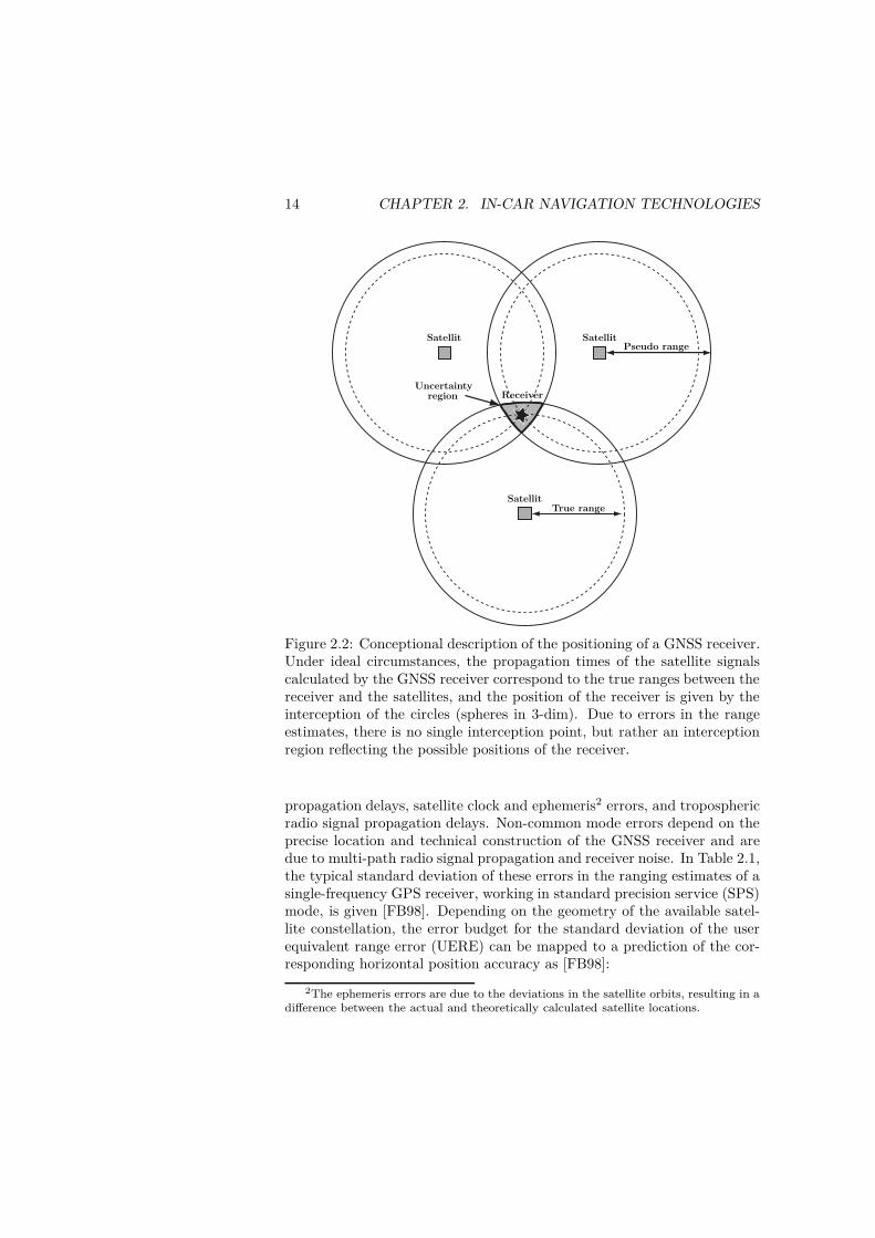
The basic operational idea of the GNSS is that receivers measure the time-of-arrival of satellite signals and compare it to the transmission time, tocalculate the signals’ propagation time. The time propagations are used toestimate the distances from the GNSS receiver to the satellites, so-calledrange estimates. From the range estimates, the GNSS receivers calculateposition by means of trilateration. This is illustrated in Figure 2.2. Theaccuracy of the position estimates is dependent on both the accuracy ofthe range measurements and the geometry of the satellites used in thetrilateration [EWP+96, MBH05].
Errors in range estimates can be grouped together, depending on theirspatial correlation, as common mode and non-common mode errors [FB98,GWA07]. Common mode errors are highly correlated between GNSS re-ceivers in a local area (50-200 km) and are due to ionospheric radio signal
1Globalnaya Navigatsionnaya Sputnikovaya Sistema.
14 CHAPTER 2. IN-CAR NAVIGATION TECHNOLOGIES
Satellit
SatellitSatellit
Receiver
True range
Pseudo range
Uncertaintyregion
Figure 2.2: Conceptional description of the positioning of a GNSS receiver.Under ideal circumstances, the propagation times of the satellite signalscalculated by the GNSS receiver correspond to the true ranges between thereceiver and the satellites, and the position of the receiver is given by theinterception of the circles (spheres in 3-dim). Due to errors in the rangeestimates, there is no single interception point, but rather an interceptionregion reflecting the possible positions of the receiver.
propagation delays, satellite clock and ephemeris2 errors, and troposphericradio signal propagation delays. Non-common mode errors depend on theprecise location and technical construction of the GNSS receiver and aredue to multi-path radio signal propagation and receiver noise. In Table 2.1,the typical standard deviation of these errors in the ranging estimates of asingle-frequency GPS receiver, working in standard precision service (SPS)mode, is given [FB98]. Depending on the geometry of the available satel-lite constellation, the error budget for the standard deviation of the userequivalent range error (UERE) can be mapped to a prediction of the cor-responding horizontal position accuracy as [FB98]:
2The ephemeris errors are due to the deviations in the satellite orbits, resulting in adifference between the actual and theoretically calculated satellite locations.

2.3. GNSS AND AUGMENTATION SYSTEMS 15
Table 2.1: Standard deviations of errors in the range measurements in asingle-frequency GPS receiver [FB98].
Error Source Standard deviation [m]Common mode
Ionospheric 7.0Clock and ephemeris 3.6Tropospheric 0.7
Non-common modeMulti-path 0.1–3.0Receiver noise 0.1–0.7
Total (UERE) 7.9–8.5CEP with a horizontal dilution of pre-cision, HDOP=1.2
6.6–7.1
CEP =√
ln 2 · HDOP ·UERE. (2.1)
Here, CEP (circular error probable) denotes the radius of a circle that con-tains 50% of the expected horizontal position errors. Further, HDOP isthe horizontal dilution of precision, reflecting the geometry of the satelliteconstellation. Refer to [Mil08, OJCL06, ORL02] for details on typical dilu-tion of precision figures for the GPS and Galileo system. It is worth notingthat (2.1) is based on several assumptions such as uncorrelated range esti-mates and circular Gaussian-distributed position estimation errors, whichmore or less hold true [Dig07]. Therefore (2.1) should only be used as arough indication of position error.
2.3.2 Augmentation Systems
Since common mode errors are the same for all GNSS receivers in a re-stricted local area, they can be compensated by having a stationary GNSSreceiver at a known location that estimates common mode errors and trans-mits correction information to rover GNSS receivers. This technology iscommonly referred to as differential GNSS (DGNSS).
The correlation of the common mode error decreases with the distancebetween the reference station and the rover unit. This will also be the casewith the system performance [LBZ05]. The problem can be solved by anetwork of reference stations over the intended coverage area. The errorsobserved by these stations are constantly sent to a central processing sta-tion, where a map of the ionospheric delay, together with ephemeris andsatellite clock corrections, is calculated. The correction map is then relayedto the user terminals (GPS and GLONASS receivers), which can calculate
16 CHAPTER 2. IN-CAR NAVIGATION TECHNOLOGIES
correction data for their specific location [EWP+96, PCSTR06]. Thereare several satellite-based augmentation systems (SBASs) that, throughgeostationary satellites, regionally provide correction information free ofcharge for the GPS and GLONASS systems. In North America, thereis the Wide Area Augmentation System (WAAS), in Europe the Euro-pean Geostationary Navigation Overlay Service (EGNOS) and in Japanthe Multi-functional Satellite Augmentation System (MSAS). Further, theGAGAN system for India and SNAS system for China are under develop-ment [PCSTR06, Dix05, GG07]. In addition to providing correction data,the SBASs also provide information regarding the integrity of the signalsfrom the various satellites. They also serve as additional satellites andthereby enhance the available satellite constellation. In [GG07], an illus-trative example of the enhancement of the HDOP for a GPS receiver in analpine canyon environment using EGNOS data is given.
All SBASs are designed to be interoperable. The geostationary satellitesof the augmentation systems transmit correction data using the L1 (1575.42MHz) frequency of the GPS system, and therefore only the software forGPS receivers has to be modified to receive correction data. Many low-cost GPS receivers are able to use correction data from the SBASs [Dix05].Test results, based on correction data from the WAAS and EGNOS sys-tems, demonstrate position accuracy in the range of 1-2 m in the horizontalplane and 2-4 m in the vertical plane at a 95% confidence interval [CL04]. Amore thorough description on how the SBASs operate and correction datais calculated can be found in [EWP+96]. It should be pointed out thatthe discussion above about performance characteristics and augmentationsystems for the GPS system has focused on single-frequency receiver units.Using dual frequency receivers and charier-phase measurements supportedby various augmentation systems, it is possible to achieve real-time posi-tion accuracy on a decimeter level [Hei00, LBZ05, Dix05, EM99, MBP99].However, the required receiver units are currently far too costly for use incommercial in-car navigation systems. In [Dix05], a discussion of the per-formance and cost of single- and two-frequency GPS receivers and variousaugment systems is presented. In [MBH05], software developed to predictthe position accuracy of a GNSS receiver along a predefined trajectory inan urban environment is described.
Even if the GNSS receivers’ positioning accuracy is enhanced by var-ious augmentation systems, the problems of poor satellite constellations,satellite signal blockages, and signal multipath propagation in urban envi-ronments remain. With the start-up of the Galileo system, the number ofaccessible satellites will increase and the probability of poor satellite geom-etry and signal blockages in urban environments will be reduced. Further,the integrity of the provided navigation solution will increase since two(three) separate systems are available for navigation [HW06]. Still, therewill be areas such as tunnels where reliable GNSS receiver navigation solu-

2.3. GNSS AND AUGMENTATION SYSTEMS 17
tions will not be available. The problem can be reduced by ground-basedstations acting as additional satellites, so-called pseudolites. By locatingthe pseudolites at favorable sites, the accuracy and continuity of the GNSSreceivers’ navigation solution can be enhanced [GWA07, LWR+02]. How-ever, usage of pseudolites has some inherent drawbacks: it only solves thecoverage problem locally, it requires an additional infrastructure, and theGNSS receiver must be designed to handle the additional pseudolite signals.
2.3.3 Integrity Monitoring
The inherent weakness of all radio signal-based navigation methods is theirreliance on information that may become erroneous, disturbed, or blockedwhile transferred from the external sources to the receiver. More precise,due to malfunctions in the software or hardware of the external sources,the transmitted information may become erroneous without any notifica-tion by the receiver. In, e.g. [BO07, OSW+03] possible GPS failure modesare listed. Further, intentionally or not, other electronic devices may ra-diate RF signals in the frequency spectrum used for the GNSS signals,causing interferences. Moreover, the environment surrounding the receivermay cause multi-path propagation, distortion and attenuation of the radiosignal, thus complicating proper signal acquisition and distorting the infor-mation accessible by the receiver. Therefore, to create a reliable and robustnavigation system, the system should incorporate integrity monitoring aswell as be combined with information from redundant sources.
There are three key components in integrity monitoring: fault detec-tion, fault isolation and removable of faulty measurements sources from thenavigation solution [HLW04]. The availability of the navigation system toperform these tasks is directly related to its integrity and continuity of ser-vice [Lee07]. Fault detection, i.e., checking for outliers and other anomaliesin the information from the sensors or subsystems, is used to timely alert ifthe calculated navigation solution is unreliable and may exceed predefinedprotection levels. Hence, it indicates if the specified minimum accuracy inthe navigation solution, required for subsequently applications, cannot bemaintained. The ability to isolate and remove the faulty information beforecontaminating the navigation solution means that the system can continueworking using the remaining information sources. Thus, the continuity ofservice of the navigation system is enhanced.
A necessity to be able to perform integrity monitoring is the avail-ability of redundant information in the system [Stu89]. For a civilianGNSS receiver this redundant information can be obtained from an aug-mentation system such the EGNOS or WAAS system [GWA07, EWP+96],by observing more satellite signals than the minimum number necessaryto compute a position estimate [Lee07, HLW04, HW06], or by a com-plimentary navigation system, such as dead-reckoning or inertial naviga-

18 CHAPTER 2. IN-CAR NAVIGATION TECHNOLOGIES
tion [BOF07a, BOF07b, BO07, MZIMGS07].The inherent weakness of integrity monitoring via an augmentation sys-
tem, such as an SBAS, is that its signals are also vulnerable to jamming, in-terference and blockage [BOF07a]. Therefore, integrity critical applicationsor systems with limited access to the signals from the augmentation sys-tem, such as electronic fee collection of land-vehicles moving in dense urbanarias, may necessitate a navigation platform that self-evaluates the integrityof the navigation solution. For GNSS receivers, self-evaluated integritymonitoring through observation of more satellite signals than necessary tocompute a position estimate is referred to as receiver autonomous integritymonitoring (RAIM). There are several different RAIM methods, e.g., therange comparison method, the least-square residual method, and the paritymethod [GWA07]. They all require a minimum of five satellites signals todetect a failure in one of the signals and signal measurements from a min-imum of six satellites to isolate the failure [HLW04, Stu89, MZIMGS07].The reliability of the detection and identification of the different RAIMalgorithms is highly dependent on the amount of redundant informationavailable and the geometry of the satellite constellation. Therefore, withthe renewal of the GLONASS system and the upcoming Galileo systemRAIM algorithms using combinations of these systems have been devel-oped, see [Lee07, HLW04, HW06]. In the simulation study of [HW06], theresults theoretically indicate that for any point on the globe a RAIM algo-rithm utilizing the signals from the GPS, GLONASS and Galileo systemstogether can detect an outlier of 20 m with a 80% probability at a 0.5%significance level and then isolate the fault with a 90% probability. Thecorresponding outlier value for the GPS alone is approximately 435 m.
Despite improvements in availability and integrity monitoring using thecombination of GNSSs, the likelihood of having access to sufficient satel-lites signals to produce a navigation solution and perform RAIM is lowin dense urban environments [MZIMGS07]. Therefore, it is necessary touse additional navigation means and aides, such as dead-reckoning, iner-tial navigation or maps-matching, to produce a reliable and robust in-carnavigation system. The information from these systems may then be usedto access the integrity of the GNSS-receiver navigation solution. However,since the sensors, etc. of the other system components are also subjected topossible failures – see e.g. [BO07] and [QON06] for possible failure modesin INS and map-matching, respectively – integrity monitoring should in-clude the full system. Integrity monitoring on a full system level is furtherdiscussed in Section 2.7 on information fusion and filter structures.

2.4. MOTION SENSORS AND COORDINATE SYSTEMS 19
Table 2.2: Sensors commonly used as a complement to GNSS-receivers forenhancement of in-car navigation systems.
Sensor MeasurementSteering encoder Front wheel directionOdometer Traveled distanceVelocity encoders Wheel velocities (indirectly. heading)Electronic compass Heading relative magnetic northAccelerometer AccelerationGyroscope (rate-gyro) Angular rotation (velocity)
2.4 Motion Sensors and Coordinate Systems
In this section, a variety of useful sensors for vehicle positioning and nav-igation is considered. To fuse the available information from the vehiclebased sensors to reliable estimates on position, velocity and attitude, a re-view of the most commonly used coordinate systems is required, which isanother topic of this section. Information processing, e.g., dead reckoningand inertial navigation, is then discussed in Section 2.5.
2.4.1 Vehicle Motion Sensors
There are a number of sensors, wheel odometers, magnetometers, accelerom-eters, etc. that can provide information about a vehicle’s state that maybe used in combination with a GNSS receiver or other absolute positioningsystem. In Table 2.2, the most commonly used sensors, together with theinformation they provide, are summarized.
A steering encoder measures the angle of the steering wheel. Hence, itprovides a measure of the angle of the front wheels relative to the forwarddirection of the vehicle platform. Together with information on the wheelspeeds of the front wheel pair, the steering angle can be used to calculatethe heading rate of the vehicle.
An odometer provides information on the traveled curvilinear distanceof a vehicle by measuring the number of full and fractional rotations of thevehicle’s wheels [AP99]. This is mainly done by an encoder that outputsan integer number of pulses for each revolution of the wheel. The numberof pulses during a time slot is then mapped to an estimate of the traveleddistance during the time slot by multiplying by a scale factor dependingon the wheel radius.
A velocity encoder provides a measurement of the vehicle’s velocity byobserving the rotation rates of the wheels. If separate encoders are usedfor the left and right wheel of either the rear or front wheel pair, or ifseparate encoders are used for the wheels on one side of the vehicle, an
20 CHAPTER 2. IN-CAR NAVIGATION TECHNOLOGIES
estimate of the heading change of the vehicle can be found through thedifference in wheel speeds. Information on the speed of the different wheelsis often available through the sensors used in the anti-lock breaking system(ABS). See [CGP02, CGP04, Hay05] for details. Though this informationis provided at no additional cost in terms of extra sensors, the generallylow resolution of the ABS sensors can seriously affect the reliability of thecalculated heading estimate. Therefore, the usage of additional wheel en-coders may be necessary to form a reliable estimate of the heading changesfrom the information about the wheel speeds.
These notions of how to estimate traveled distance, velocity and headingof the vehicle are all based on the assumption that wheel revolutions canbe translated into linear displacements relative to the ground. However,there are several sources of inaccuracy in the translation of wheel encoderreadings to traveled distance, velocity and heading change of the vehicle.They are [AP99, CGP04, BF96]:
• Wheel slips
• Uneven road surfaces
• Skidding
• Changes in wheel diameter due to variations in temperature, pressure,tread wear and speed
• Unequal wheel diameters between the different wheels
• Uncertainties in efficient wheelbase (track width)
• Limited resolution and sample rate of the wheel encoders
The first three error sources are terrain dependent and occur in a non-systematic way. This makes it difficult to predict and limit their negativeeffect on the accuracy of the estimated traveled distance, velocity and head-ing. The four remaining error sources occur in a systematic way, and theirimpact on the traveled distance, velocity and heading estimates are moreeasily predicted. The errors due to changes in wheel diameter, unequalwheel diameter and uncertainties in efficient wheelbase can be reduced byincluding them as parameters estimated in the sensor integration.
An electronic compass is an electronic device, constructed from mag-netometers, that provides heading measurements relative to the Earth’smagnetic north by observing the direction of the Earth’s local magneticfield [AP99]. To convert the compass heading into an actual north heading,the declination angle (i.e., the angle between the geographic and magneticnorth) is needed, which is position dependent. Thus, knowledge of the com-pass position is necessary to calculate the heading relative to geographicnorth.

2.4. MOTION SENSORS AND COORDINATE SYSTEMS 21
Generally, the compass is constructed around three magneto-resistiveor flux-gate magnetometers, together with pitch and roll sensors [TW04].The pitch and roll measurements are needed to determine the attitudebetween the coordinate system spanned by the magnetic sensors sensitivityaxes and the local horizontal plane, so that the horizontal component ofthe Earth’s magnetic field can be calculated. For a vehicle moving in aplanar environment experiencing only small pitch and roll angles, a compassconstructed from only two magnetometers with perpendicular sensitivityaxes lying approximately in the horizontal plane may be sufficient andcost-effective. In [TW04] and [Pet86], details about compasses based onflux-gate magnetometers can be found. A review of magnetic sensors isfound in [Len90].
Power lines and metal structures such as bridges and buildings alongthe trajectory of the vehicle cause variations in the local magnetic field,resulting in large and unpredictable errors in the heading estimates of thecompass. Therefore, the usefulness of magnetic compasses in in-car naviga-tion systems can be questioned [AP99]. However, there are other applica-tions of magnetic sensors in in-car navigation systems. See [YF03], wheremagnetic sensors are used to detect the vehicle’s location with the help ofmagnets distributed along a highway.
An accelerometer provides information about the acceleration of theobject to which it is attached. More strictly speaking, an accelerome-ter produces an output proportional to the specific force exerted on theinstrument,3 projected onto the coordinate frame mechanized by the ac-celerometer [Bri71]. Information about an object’s orientation and rotationmay be obtained using a gyroscope (rate-gyro), which measures the angularrotation (velocity) of the object relative to the inertial frame of reference.Hence, by equipping the vehicle with inertial sensors, i.e., accelerometersand gyroscopes, information about the vehicle’s acceleration and rotationis obtained and can be mapped into estimates of the vehicle’s attitude,velocity and position.
There are many different ways to construct inertial sensors. In [TW04],a description of common technologies and their typical performance param-eters can be found. A description of the trends in inertial sensor technologyis offered in [BS01]. Historically, inertial sensors have mostly been used inhigh-end navigation systems for missile, aircraft and marine applicationsdue to the high cost, size and power consumption of the sensors. However,with the progress in micro-electromechanical-system (MEMS) sensor tech-nology it has become possible to construct inertial sensors meeting the costand size demands needed for low-cost commercial electronics, such as vehi-
3According to the principle of equivalence, it is impossible to instantaneously distin-guish between gravitational and inertial forces. Hence, the output of an accelerometercontains both forces, referred to as the specific force.

22 CHAPTER 2. IN-CAR NAVIGATION TECHNOLOGIES
cle navigation systems. However, the price paid (with currently availablesensors) is a reduced performance characteristic. An illustrative descrip-tion of developments in MEMS technology and its many applications isoffered in [BRB+06]. In chapter 7 of [TW04], an introduction to MEMSinertial sensor technology can be found. In [ESN07], a discussion of theusefulness of MEMS sensors in vehicle navigation and their limitations ispresented. Their usefulness in navigation primarily depends on MEMSgyroscope development.
Unlike odometers, velocity encoders, and magnetic compasses, whoseerrors are partly related to the terrain in which the vehicle is traveling,inertial sensors are fully self-contained. However there are several errorsources associated with inertial sensors which must be considered. Someof the most significant inertial sensor errors can be categorized as [TW04,GWA07]:
• Biases
• Scale factors
• Nonlinearities
• Noise
The bias error occurs as non-zero output from the sensor for a zero input.Scale factor and nonlinearity errors describe the uncertainty in linear andnon-linear scaling between the input and output, respectively. Each of theseerror categories in general includes some or all of the following components:
• Fixed terms
• Turn-on to turn-on varying terms
• Random walk terms
• Temperature varying terms
The fixed terms, and to a large extent the temperature varying terms,can be estimated and compensated by calibration of the sensors; referto [Cha97, Rog03, ASNES06, SH06a, FON08, SAG+07] for several cali-bration approaches. Turn-on to turn-on terms differ from time to timewhen the sensor is turned on, but stay constant during the operation time,whereas the random walk error slowly varies over time. The sensors’ turn-on to turn-on and random walk error characteristics are therefore of majorconcern in the choice of sensors and information fusion method. Besidesthe error components discussed above, there are also error components dueto the inevitable imprecision in the mounting of the sensors as well as mo-tion dependent error components, which maybe necessary to consider in

2.4. MOTION SENSORS AND COORDINATE SYSTEMS 23
the choice of sensors and information fusion algorithms. Refer to [Far07]for details on inertial instrumentation error characterization.
In order to measure the vehicle’s dynamics in both long- and cross-track directions, a cluster of inertial sensors is needed, referred to as aninertial sensor assembly (ISA). Depending on the construction of the navi-gation system, the ISA may consist of solely accelerometers, but more fre-quently a combination of accelerometers and gyroscopes is used. See [TP05]and [CLD94] for examples of all accelerometer-based navigation systems.In general, a six-degree-of-freedom ISA, i.e., an inertial measurement unit(IMU) designed for unconstrained navigation in three dimensions, consistsof three accelerometers and three gyroscopes, where the sensitivity axesof the accelerometers are mounted to be orthogonal and span a three-dimensional space, and the gyroscopes measure the rotations around theseaxes.
2.4.2 Coordinate Systems
Before continuing with a discussion on how the information supplied byvehicle mounted sensors is processed into an estimate of the vehicle’s posi-tion, velocity, and attitude, or is exchanged with the interfacing informationsources in the system, it is essential to introduce a few coordinate systems:the vehicle coordinate system, the earth centered inertial (ECI) coordinatesystem, the earth centered earth fixed (ECEF) coordinate system and thegeographic coordinate system.
The vehicle coordinate system, sometimes referred to as the body coordi-nates, is the coordinate system associated with the vehicle. Commonly, butnot necessarily, it has its origin at the center of gravity of the vehicle, andthe coordinate axes are aligned with the forward, sideways (to the right)and down directions associated with the vehicle. The information providedby vehicle mounted sensors and the motion and dynamic constraints im-posed by the vehicle model are generally expressed with reference to thiscoordinate system.
The earth centered inertial coordinate system is the favored inertial co-ordinate system for navigation in a near-earth environment [GWA07]. Theorigin of the ECI coordinate system is located at the center of gravity of theEarth (viz. a geocentric coordinate system). Its z-axis is aligned with thespin axis of the Earth, the x-axis points towards the vernal equinox, andthe y-axis completes the right hand orthogonal coordinate system. This isillustrated in Figure 2.3. The accelerations and angular velocities observedby the inertial sensors are measured relative to this coordinate system.
Closely related to the ECI coordinate system is the geocentric earth cen-tered earth fixed coordinate system, which also has its origin at the center ofgravity of the Earth but rotates with the Earth. Its first coordinate axis (x-axis) lies in the intersection between the primer meridian and the equator

24 CHAPTER 2. IN-CAR NAVIGATION TECHNOLOGIES
Equator
Referencemeridian
Geographic frame
North
East
Down
Latitude
Longitude
FocusVernalequinox
zi ≡ ze
yi
xi
ye
xe
Earth rotation
Figure 2.3: Illustration of the earth centered earth fixed frame (axes de-noted by the superscript e), the geographic frame (axes denoted North,East and Down), and the earth centered inertial coordinate frame (axesdenoted by the superscript i).
plane, the z-axis is parallel to the spin axis of the Earth, and the y-axis com-pletes the right hand orthogonal coordinate system. Refer to Figure 2.3 foran illustration. Nearly related to the geocentric ECEF coordinate systemis the geodetic coordinate system defined by the World Geodetic System(WGS) 84 datum, commonly referred to as the geodetic ECEF coordinatesystem. Details on the coordinate transformation between these two sys-tems are found in [FB98]. A geodetic coordinate system representation isbased on an approximation of the Earth geoid (globally or locally) by anellipsoid that rotates around its minor axis [Zha97]. A location in the co-ordinate system is described in terms of the longitude and latitude anglesmeasured with respect to the equatorial and meridional plan associatedwith the reference ellipsoid. The parameters of the reference ellipsoid, such

2.5. INFORMATION PROCESSING 25
as shape, size, orientation, etc., define the datum of the coordinate sys-tem. Refer to [Zha97, DR98] for details on reference coordinate systemsand different datums. The coordinate system defined by WGS 84 is thecoordinate system used in the GPS.
The geographic coordinate system is a local coordinate frame whoseorigin is the projection of the vehicle coordinate system origin onto theEarth’s geoid. The x-axis points towards true north, the y-axis to theeast and z-axis completes the right hand orthogonal coordinate systempointing towards the interior of the Earth perpendicular to the referenceellipsoid [Bri71]. The coordinate system is illustrated in Figure 2.3. (Notethat the z-axis does not point towards the center of Earth but rather alongthe ellipsoid normally towards one of its foci.) The geographic coordinatesystem is generally used as a reference when expressing the velocity com-ponents of the vehicle’s motion and the attitude of the vehicle platform.The vehicle attitude is commonly described by the three Euler angles – roll,pitch and yaw – relating the vehicle and geographic coordinate systems toeach other.
Detailed descriptions of the various coordinate systems used in naviga-tion, together with common coordinate transformations, are found in thestandard textbooks on inertial navigation [Bri71, FB98, TW04, GWA07,Cha97, Rog03].
2.5 Information Processing
Processing of information from vehicle based sensors to estimate position,velocity and attitude is discussed in this section.
2.5.1 Dead Reckoning
Velocity encoders, accelerometers and gyroscopes all provide informationon the first or second order derivative of the position and attitude of thevehicle. Further, the odometer gives information on the traveled distanceof the navigation system. Hence, except for the magnetometer, all themeasurements of the sensors in Table 2.2 only contain information on therelative movement of the vehicle and no absolute positioning or attitudeinformation. The translation of these sensor measurements into positionand attitude estimates will therefore be of an integrative nature requiringthat the initial state of the vehicle is known, and for which measurementerrors will accumulate with time or, for the odometer, with the traveled dis-tance. Moreover, the information provided by the vehicle mounted sensoris, except from possible fixed rotations, represented in the vehicle coordi-nate system. Therefore, before the sensor measurements are processed intoa position, velocity and attitude estimate, they must be transformed intoa coordinate system where they are more easily interpreted, preferably the
26 CHAPTER 2. IN-CAR NAVIGATION TECHNOLOGIES
ECEF or the geographic coordinate system. Moreover, if the sensor mea-surements are to be used in combination with information provided byother information sources, they must be expressed in a common coordinatesystem.
The process of transforming the measurements from the vehicle mountedsensor into an estimate of the vehicles position and attitude is generallyreferred to as DR, or if only involving inertial sensors inertial navigation.The process of DR (and inertial navigation) can briefly be described as:
1. The gyroscope, compass or differences in wheel speed measurementsare used to determine the attitude (3-dim) or heading (2-dim) of thevehicle.
2. Attitude (or heading) information is then used to project the in-vehicle coordinates measured acceleration, velocity or traveled dis-tance onto the coordinate axes of the preferred navigation coordinatessystem, e.g., the ECEF or geographic coordinate frame.
3. Traveled distance, velocity or acceleration is then integrated over timeto obtain position and velocity estimates in the navigation coordinateframe.
Refer to [OLS07, OLS06, CGP02, CGP04] for details on how dead reckoningis done in vehicle navigation systems.
2.5.2 Inertial Navigation
In Figure 2.4, a block diagram of a strap-down4 inertial navigation system(INS) is shown. The INS comprises two distinct parts, the IMU and thecomputational unit. The former provides information on the accelerationsand angular velocities of the navigation platform relative to the inertialcoordinate frame of reference, preferably the ECI coordinate system. Theangular rotations (rates) observed by the gyroscopes are used to track therelation between vehicle coordinate system and the navigation coordinateframe of choice, commonly the ECEF or geographic coordinate frame. Thisinformation is then used to transform the specific force observed in vehi-cle coordinates into the navigation frame, where the gravity accelerationis subtracted from the observed specific force. What remains are the ac-celerations in the navigation coordinates. To obtain the position of thevehicle, the accelerations are integrated twice with respect to time; refer to[Bri71, FB98, TW04, GWA07, Cha97, Rog03, Sav98a, Sav98b, KGG+83]

2.5. INFORMATION PROCESSING 27
INS
Position
Velocity
Attitude
Attitude
Coordinaterotation
determinationGyro-scopes
Accelero-meters
Sens
orer
ror
com
pen
sati
on
Gravity
model
IMU
Navigation equations
∫dt
∫dt
+ −+
Figure 2.4: Conceptional sketch of a strap-down INS. The dash arrowsindicate possible points for insertion of calibration (aiding) data.
for a thorough treatment of the subject of inertial navigation. In [Std01,CATB04], details on inertial sensors and systems terminology can be found.
The integrative nature of the navigation calculations in DR and inertialnavigation systems gives the systems a low-pass filter characteristic thatsuppresses high-frequency sensor errors but amplifies low-frequency sensorerrors. This results in a position error that grows without bound as afunction of the operation time or traveled distance, and where the errorgrowth depends on the error characteristics of the sensors. In general, itholds that for an INS a bias in the accelerometer measurements causes er-ror growth proportional to the square of the operation time, and a bias inthe gyroscopes causes error growth proportional to the cube of the opera-tion time [ESN07, TP05, SNDW99, DSNDW01]. The detrimental effect ofgyroscope errors on the navigation solution is due to the direct reflectionsof the errors on the estimated attitude. The attitude is used to calculatethe current gravity force in navigation coordinates and cancel its effecton the accelerometer measurements. Since in most land vehicle applica-tions the vehicle’s accelerations are significantly smaller than the gravityacceleration, small errors in attitude may cause large errors in estimatedaccelerations. These errors are then accumulated in the velocity and po-sition calculations. Hence, the error characteristics of the gyroscopes usedin the IMU are of major concern when designing an INS.
To summarize, the properties of DRSs and INSs are complimentaryto those of the GNSSs and other radio-based navigation systems. Theseproperties are:
• They are self-contained, i.e., they do not rely on any external source
4The term strap-down refers to the fact that the gyroscopes and accelerometers arerigidly attached to the navigation platform. In a gimballed INS, the sensors are mountedon a platform isolated from the rotations of the vehicle [GWA07].
28 CHAPTER 2. IN-CAR NAVIGATION TECHNOLOGIES
of information that can be disturbed or blocked.
• The update rate and dynamic bandwidth of the systems are mainlyset by the system’s computational power and the bandwidth of thesensors.
• The integrative nature of the systems results in a position error thatgrows without bound as a function of the operation time or traveleddistance.
Contrary to these properties, the GNSS and other radio-based navigationsystems give position and velocity estimates with a bounded error but ata relatively low rate and depend on information from an external sourcethat may be disturbed. The complimentary features of the two types ofsystems make their integration favorable and if properly done results innavigation systems with higher update rates, accuracy, integrity and abilityto provide a more continuous navigation solution under various conditionsand environments.
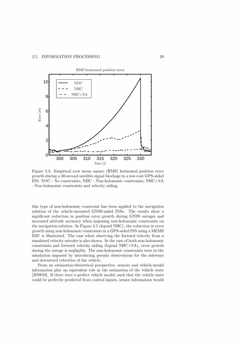
Odometers and velocity and steering encoders have proven to be veryreliable DR sensors. For movements in a planar environment, they can pro-vide reliable navigation solutions during several minutes of GNSS outages.However, in environments that significantly violate the assumption of aplanar environment, accuracy is drastically reduced [DSNDW01]. An INSconstructed around a full-six-degree-of-freedom IMU does not include anyassumption of the motion of the navigation system and therefore is indepen-dent of the terrain in which vehicle is traveling. Moreover, it provides three-dimensional position, velocity and attitude information. In combinationwith decreasing cost, power consumption and size of the MEMS inertial sen-sors, this makes vehicle navigation systems incorporating MEMS IMUs at-tractive. However, current ultra low-cost MEMS inertial sensors have an er-ror characteristic causing position errors in the range of tens of meters dur-ing 30 seconds of stand-alone operation [BL04, GC07, ESN07, NNGES07].This is also illustrated in Figure 2.5 (legend NOC), where the root meansquare (RMS) horizontal position error during a 30-second GNSS signaloutage in a GNSS-aided INS is shown. In the simulation, the IMU sensorswere modeled as ideal sensors, except that measurement noises, turn-onto turn-on and time varying biases reflect current ultra low-cost MEMSinertial sensors were added.
2.5.3 Vehicle Models and Motions
Under ideal conditions, a vehicle moving in a planar environment experi-ences no wheel slip and no motions in the direction perpendicular to theroad surface. Thus, in vehicle coordinates, the downward and sideways ve-locity components should be close to zero. In [GC07, ESN07, DSNDW01],
2.5. INFORMATION PROCESSING 29
300 305 310 315 320 325 3300
2
4
6
8
10
RMS horizontal position error
Err
or[m
]
Time [s]
NOC
NHC
NHC+VA
Figure 2.5: Empirical root mean square (RMS) horizontal position errorgrowth during a 30-second satellite signal blockage in a low-cost GPS-aidedINS. NOC - No constraints, NHC - Non-holonomic constraints, NHC+VA- Non-holonomic constraints and velocity aiding.
this type of non-holonomic constraint has been applied to the navigationsolution of the vehicle-mounted GNSS-aided INSs. The results show asignificant reduction in position error growth during GNSS outages andincreased attitude accuracy when imposing non-holonomic constraints onthe navigation solution. In Figure 2.5 (legend NHC), the reduction in errorgrowth using non-holonomic constraints in a GPS-aided INS using a MEMSIMU is illustrated. The case when observing the forward velocity from asimulated velocity encoder is also shown. In the case of both non-holonomicconstraints and forward velocity aiding (legend NHC+VA), error growthduring the outage is negligible. The non-holonomic constraints were in thesimulation imposed by introducing pseudo observations for the sidewaysand downward velocities of the vehicle.
From an estimation-theoretical perspective, sensors and vehicle-modelinformation play an equivalent role in the estimation of the vehicle state[JDW03]. If there were a perfect vehicle model, such that the vehicle statecould be perfectly predicted from control inputs, sensor information would

30 CHAPTER 2. IN-CAR NAVIGATION TECHNOLOGIES
be superfluous. Contrarily, if there were such things as perfect sensors, thevehicle model would provide no additional information. Neither of theseextremes exists. It is clear, however, that navigation system performancecan be enhanced by utilizing vehicle models. Moreover, the incorporationof a vehicle model in the navigation system may allow the use of less costlysensors without degradation in navigation performance.
There are numerous vehicle model and motion constraints, ranging fromthe above-mentioned non-holonomic constraints to more advanced modelsincorporating wheel slip, tire stiffness, etc. Different vehicle models andconstraints of varying complexity can be found in [JDW03, HT06, ESN07,DSNDW01, BRG06, MZIMGS07, JDW95, RS07]. In [JDW03], a theo-retical framework for analyzing the impact of various vehicle models isdeveloped. The results show that there is a lot to gain from using morerefined vehicle models, especially in the accuracy of the orientation esti-mate. However, it is difficult to find good vehicle models independent of thedriving situation [MZIMGS07]. More advanced models require knowledgeabout several parameters such as vehicle type, tires, and environmentalspecifics [DSNDW01]. To adapt the model to different driving conditions,these parameters must be estimated in real-time. Alternatively, the drivingconditions must be detected and used to switch between different vehiclemodels. An example of this, using an interactive multimodel extendedKalman filter, can be found in [MZIMGS07].
2.6 Map Information
Position information in terms of pure coordinates is often difficult to inter-pret for a driver. To assist the driver in relating the position informationto a physical location, the in-car navigation system commonly displays thevehicle’s position on a map. Moreover, under normal conditions, the lo-cation and trajectory of a car is restricted by the road network. Hence, adigital map of the road network can be used to impose constraints on thenavigation solution of the in-car navigation system, a process referred toas map-matching [QON06].
2.6.1 Digital Maps and Spatial Road WorkRepresentation
The digital maps used in in-car navigation systems differ quite substantiallyfrom ”classical” printed or digitalized maps in the way they are represented.These maps can be seen as an image built up of a set of pixels, which iseasy for the human to interpret. For a computer trying to match thevehicle location on the street network, and to compute a recommendedpath, the image contains little information. The digital maps used in-
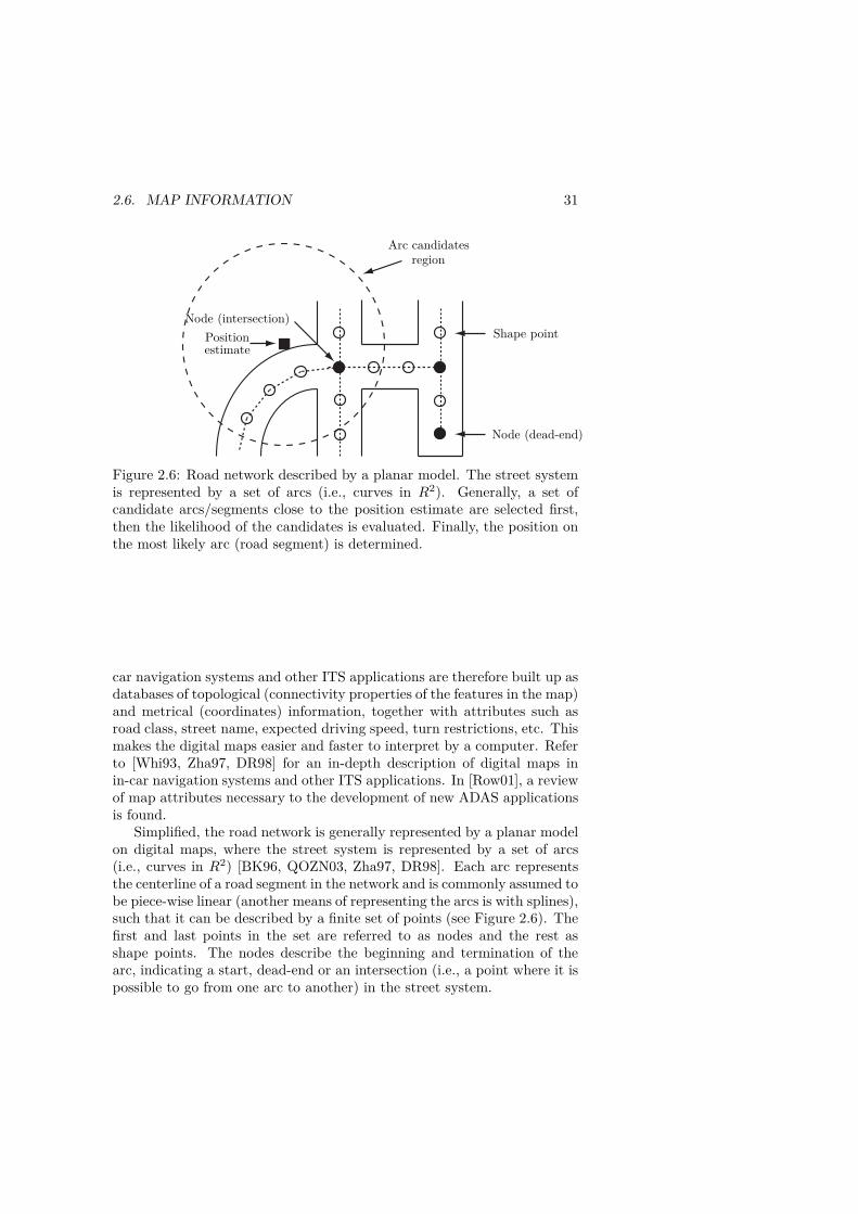
2.6. MAP INFORMATION 31
Node (intersection)Shape point
Node (dead-end)
Positionestimate
Arc candidatesregion
Figure 2.6: Road network described by a planar model. The street systemis represented by a set of arcs (i.e., curves in R2). Generally, a set ofcandidate arcs/segments close to the position estimate are selected first,then the likelihood of the candidates is evaluated. Finally, the position onthe most likely arc (road segment) is determined.
car navigation systems and other ITS applications are therefore built up asdatabases of topological (connectivity properties of the features in the map)and metrical (coordinates) information, together with attributes such asroad class, street name, expected driving speed, turn restrictions, etc. Thismakes the digital maps easier and faster to interpret by a computer. Referto [Whi93, Zha97, DR98] for an in-depth description of digital maps inin-car navigation systems and other ITS applications. In [Row01], a reviewof map attributes necessary to the development of new ADAS applicationsis found.
Simplified, the road network is generally represented by a planar modelon digital maps, where the street system is represented by a set of arcs(i.e., curves in R2) [BK96, QOZN03, Zha97, DR98]. Each arc representsthe centerline of a road segment in the network and is commonly assumed tobe piece-wise linear (another means of representing the arcs is with splines),such that it can be described by a finite set of points (see Figure 2.6). Thefirst and last points in the set are referred to as nodes and the rest asshape points. The nodes describe the beginning and termination of thearc, indicating a start, dead-end or an intersection (i.e., a point where it ispossible to go from one arc to another) in the street system.

32 CHAPTER 2. IN-CAR NAVIGATION TECHNOLOGIES
2.6.2 Map-Matching
Matching the output of the navigation system to the road network ofthe digital map generally involves three steps. First, a set of candidatearcs or segments are selected. Second, the likelihood of the candidatearcs/segments is evaluated using geometrical and topological informationas well as the correlation between the trajectory history of the vehicle andthe candidate paths in the map. Finally, the vehicle location on the mostlikely road segment is determined.
The geometrical information includes measures such as the closenessbetween the position estimate and nearest road on the map, the differencein heading as indicated by the navigation system and road segments ofconcern, and the difference in the shape of the road segments with respectto estimated trajectory. Refer to [BK96] for a discussion and descriptionof common measures such as point-to-point, point-to-curve and curve-to-curve matching to extract geometrical information. The topological infor-mation criterion determines the connectivity of the candidate roads (arcs),e.g., the vehicle cannot suddenly move from one road segment to another ifthere is no intersection point between the segments. The likelihood of theroad segment candidates is found by assigning different weights to the geo-metrical and topological information measures and combining them. Referto [OLS07, ENB05, ENB07, QOZN03, KK01, BJD07, Zha97, ZWW07] forvarious weighting and combining approaches such as belief theory, fuzzynetwork and state machines. In [QON07], a survey of state-of-the art map-matching algorithms is found, together with ideas on further research di-rections.
Traditionally, map-matching has been a unidirectional process, wherethe position and trajectory estimated by the GNSS receiver, vehicle motionsensors and vehicle model information have been used as input to produce aposition and trajectory consistent with the road network of the digital map.With improved map quality, the possibility of a bidirectional informationflow in the map-matching has become feasible, viewing the map informationas ”observations” in the estimation of the information fusion [WSM+05].That is, the heading, length, etc. of the road segment identified by the map-matching algorithm can be compared to the navigation solution and usedto calibrate the sensors in the system [Zha97]. This type of bidirectionalmap-matching is found in [SC97, ENB05, ENB07, GGB+02]. In [LTK05],a scheme for map-matching is examined, where the pseudo ranges, and notthe position estimates, from the GNSS receiver are used together with aterrain map as the input for the mapping algorithm. The result is notonly a higher accuracy of the position estimates but also the possibility toobtain a navigation solution when less than four satellites are available.
A series of decisions, such as map scale, map projection and datum, areinvolved in the creation of a map and influence its quality and accuracy.

2.7. INFORMATION FUSION 33
Further, the digitalization and identification process in the construction ofthe spatial road network in the digital map causes additional errors. Theseerrors can be categorized as topological or geometrical, where topologicalerrors originate from the fact that features such as roundabouts, junctions,medians, curves, etc. of the real world have been omitted, missed or sim-plified in the creation of the digital map [QON06, QON07]. Geometricalerrors arise from displacements of map features, such as road centerlines,junctions, etc. from their actual location. The cumulative effect of these er-rors influences the accuracy of the map and causes an inherent uncertaintylevel in the map-matching process. To establish a high level of confidence(integrity) in the system, it is essential to constantly quantify reliabilityand look for anomalies in the result of the map-matching. In [QON06], anempirical approach to evaluate the integrity of the map-matching is there-fore developed. In [QON07, CLYC05, ZWW03], the effects of sensor errorsand map quality on the map-matching are analyzed. Refer to [Gru08] for afew critical comments regarding the integrity of map-matching in road-usecharging systems.
2.7 Information Fusion
The objective of information fusion is to obtain more information thanis present in any individual information source by combining informationfrom different sources [YLZ07]. In practice, this means that by utilizingthe complimentary properties of the different information sources, the in-formation fusion tries to reduce ambiguities in the measured informationand thereby expand the spatial and temporal coverage in which the systemworks and enhance the reliability of the system.
2.7.1 Filter Structures
The key component in information fusion is in the concept of navigation,to produce estimates of the vehicle’s position, velocity, etc. from the sen-sor measurements [YLZ07]. The state estimation can be realized basicallyin two ways, the centralized filtering mode and the decentralized filteringmode [Jek00], where the choice of mode is related to the system require-ments regarding estimation accuracy, computational complexity, possibilityof fault detection and fault removal.
In the centralized filter mode, the raw measurements from all informa-tion sources are processed and combined in one filter to produce a naviga-tion solution. The centralized filtering structure is illustrated in Figure 2.7.The centralized filtering mode has the benefit of minimal information loss,so that all the information is directly available to the filter, which if properlydesigned and assigned with correct prior information theoretically shouldproduce an optimal state estimate [SD04]. However, the computational
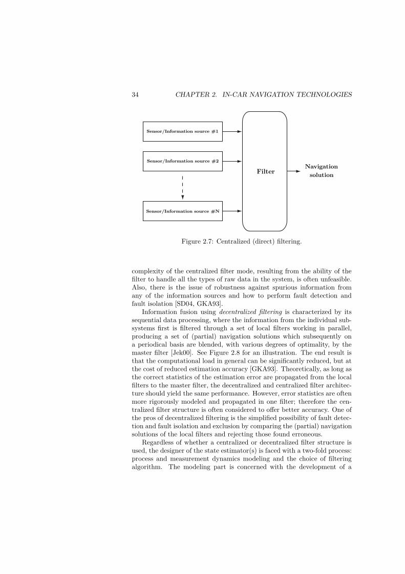
34 CHAPTER 2. IN-CAR NAVIGATION TECHNOLOGIES
Sensor/Information source #1
Sensor/Information source #2
Sensor/Information source #N
FilterNavigation
solution
Figure 2.7: Centralized (direct) filtering.
complexity of the centralized filter mode, resulting from the ability of thefilter to handle all the types of raw data in the system, is often unfeasible.Also, there is the issue of robustness against spurious information fromany of the information sources and how to perform fault detection andfault isolation [SD04, GKA93].
Information fusion using decentralized filtering is characterized by itssequential data processing, where the information from the individual sub-systems first is filtered through a set of local filters working in parallel,producing a set of (partial) navigation solutions which subsequently ona periodical basis are blended, with various degrees of optimality, by themaster filter [Jek00]. See Figure 2.8 for an illustration. The end result isthat the computational load in general can be significantly reduced, but atthe cost of reduced estimation accuracy [GKA93]. Theoretically, as long asthe correct statistics of the estimation error are propagated from the localfilters to the master filter, the decentralized and centralized filter architec-ture should yield the same performance. However, error statistics are oftenmore rigorously modeled and propagated in one filter; therefore the cen-tralized filter structure is often considered to offer better accuracy. One ofthe pros of decentralized filtering is the simplified possibility of fault detec-tion and fault isolation and exclusion by comparing the (partial) navigationsolutions of the local filters and rejecting those found erroneous.
Regardless of whether a centralized or decentralized filter structure isused, the designer of the state estimator(s) is faced with a two-fold process:process and measurement dynamics modeling and the choice of filteringalgorithm. The modeling part is concerned with the development of a

2.7. INFORMATION FUSION 35
Sensor/Information source #1
Sensor/Information source #2
Sensor/Information source #N
Local filter
Local filter
Local filter
Master filter
Raw
data
Part
ial
nav
igati
on
solu
tio
ns
Navigation
solution
Figure 2.8: Decentralized filtering.
model that consistently and in a framework suitable for the state estimator(filter) describes the process and measurement dynamics of the navigationsystem, together with a proper description of the process and measurementnoise statistics. The model must be complete enough to give an adequatedescription of the system and at the same time be sufficiently simple for thefiltering algorithm to become computationally feasible [GS69]. The choiceof filter algorithm is then a balance between computational complexity,robustness against modeling errors and accuracy of the algorithm. Sincenonlinear process and measurement models generally are used to describeinformation observations and vehicle dynamics, the proceeding discussionon filter algorithms will focus on nonlinear filtering methods.
2.7.2 Filter Algorithms
The most widely used nonlinear filtering approach, due to its simplicity, isthe extended Kalman filter (EKF) in its various varieties. The idea behindthe EKF is to linearize the navigation and observation equations aroundthe current navigation solution and turn the nonlinear filtering probleminto a linear problem. Assuming Gaussian distributed noise sources, theminimum mean square error (MMSE) solution to the linear problem isthen provided by the Kalman filter [KSH99]. For non-Gaussian distributednoise sources, the Kalman filter provides the linear MMSE solution to thefiltering problem.
Unfortunately, the linearization in the EKF means that the originalproblem is transformed into an approximated problem which is solved op-timally, rather than approximating the solution to the correct problem.This can seriously affect the accuracy of the obtained solution or lead todivergence of the system. Therefore, in systems of a highly nonlinear na-

36 CHAPTER 2. IN-CAR NAVIGATION TECHNOLOGIES
ture and non-Gaussian noise sources, more refined nonlinear filtering ap-proaches such as Sigma-Point filters (Unscented Kalman filters), particlefilters (sequential Monte Carlo methods) and exact recursive nonlinear fil-ters, which keep the nonlinear structure of the problem, may significantlyimprove system performance [MWJ04, Dau05]. The inherent weakness ofthese nonlinear filtering approaches is the curse of dimensionality. That is,the computational complexity of the filter usually grows exponentially withthe dimension of the state vector being estimated [Dau05]. Therefore, evenwith today’s computational capacity, nonlinear filters can be unfeasible fornavigation systems with high-dimensional state vectors. However, since thenavigation equations in many navigation systems are only partial nonlin-ear, the filtering problem can be divided into a linear and nonlinear part,where the linear part, under the assumption of Gaussian-distributed noiseentries, may be solved using a Kalman filter, hence reducing the computa-tional complexity of the system [SGN05, KSG05]. A short introduction tononlinear filtering and the advantages and disadvantages of various algo-rithms are given in [Dau05].
Originating from the field of nonlinear systems and control theory, theidea of constructing a filter with a nonlinear observer is sometimes usedto blend the information from different subsystems and sensors. Referto [BMR06, ZS05, YLP04] for details. Compared to EKF algorithms forwhich there is no guaranty of convergence, the framework in which thenonlinear observer is derived often provides strong results on the region ofconvergence.
All filters discussed so far rely on an adequate system model togetherwith proper prior knowledge of the noise statistics, which can be difficultand time consuming to find. If there is a lack of accurate noise statistics,adaptive filters which try to optimize the filter parameters reflecting thenoise properties are sometimes used; refer to [MS99, HLES07, GW07] fordetails. Another approach, avoiding the need for the designer to specify asystem model at all, is the usage of a neural network to fuse the informationin the system. A neural network consists of several layers of interconnectednodes (neurons). Through a learning process where layers and intercon-nections are rearranged, the neural network is trained to develop an ade-quate system model, later used to fuse the information from the differentsensors/subsystems [Zha97]. Refer to [WG04, SN06, SNOES05, NOES04,HC08, STTN07, SN07, KEE07, PION08, CH08] for more information.
In Table 2.3, a list of filter algorithms, together with comments onestimation accuracy, computational complexity and reference to differentpapers using the filters in navigation and tracking contexts, is presented.
To quantify the efficiency and robustness of the chosen process modeland filter algorithm two major analytical tools are available, the PosteriorCram´er Rao Bound (PCRB) for the filtering problem and a sensitivityanalysis. The PCRB provides a lower bound on the mean square error
2.7. INFORMATION FUSION 37
for the filtering problem, against which the filter algorithms are evaluated.Refer to [TMN98, Ker89, Ber99] for more details. However, the meansquare error lower bound provided by the PCRB is only valid when theinput data to the filter is generated according to the system model usedin the PCRB. To quantify the effect of the choice of system model as wellas the filtering algorithm, a sensitivity analysis may be performed. Referto [GS69, BS71, GS68, JDW03, AP99] for details on sensitivity analyzes ofKalman filter and Extended Kalman filter algorithms.
2.7.3 Information Fusion in Systems Including a GNSSReceiver
Without doubt the GNSS receiver is and will remain a major componentin most vehicle navigation systems, often in combination with various ve-hicle dynamic sensors. The information fusion between GNSS receiversand other vehicle dynamic sensors, especially inertial sensors, has thereforereceived a considerable amount of interest and deserves special attention.
Depending on information flows and at what level the information isexchanged and blended between the GNSS receiver and other componentsin the integrated system, the system architectures are commonly referredto as loosely coupled, tightly coupled, ultra tightly coupled or deeply in-tegrated. However, no distinct bounds between the different systems existand the classification of integration architectures in the literature is notconsistent [BO07].
In a loosely coupled system architecture, the information exchange be-tween the GNSS receiver and other system components is unidirectionaland the navigation solution (position, velocity, etc.) of the two sub sys-tems is blended. Generally, the information provided by the GNSS receiveris used to aid the other system components, even though the reverse is alsopossible. This system architecture benefits from its simplicity but has someinherent drawbacks. Due to the filter inside the GNSS receiver, the posi-tion and velocity estimates from the GNSS receiver will be correlated inspace and time and with a structure most likely unknown to the infor-mation fusion algorithm designer [FB98]. Thus, the (correct) statistics onthe estimation error are not available for the master fusion filter, leadingto suboptimal performance. Further, no information is gained from theGNSS receiver in situations when there are not enough satellite signals forthe GNSS receiver to produce a navigation solution on its own.
In a tightly coupled system architecture, the information flow betweenthe GNSS receiver and the other system components is still unidirectional,but instead of using the navigation solution from the GNSS receiver as inputfor the fusion algorithm, basic GNSS observations (pseudo range, carrierphase or Doppler shift estimates) are used. This has several benefits. Thebasic GNSS observations are not as correlated as the position and velocity
38 CHAPTER 2. IN-CAR NAVIGATION TECHNOLOGIES
solutions calculated in the GNSS receiver, and with better known statistics,leading to higher accuracy of the integrated system [AAR03]. Further, byaccessing the signals from individual satellites, information is gained fromthe GNSS receiver even in situations when a navigation solution solelybased on GNSS observations is not possible. The integrity and continuityof service of the system also benefit from the access to individual satellitesignals, since fault detection at the signal level means that the individualsatellite signals can be rejected instead of the full navigation solution of theGNSS receiver [BO07]. This is especially important for systems using lowcost vehicle sensors, which may work alone only during a shorter durationof time without the aid of the GNSS receiver. A thorough treatment ofintegrity with respect to system architectures in GNSS-aided INSs is foundin [BO07, BOF07a, BOF07b].
By allowing a bidirectional information flow, so that the navigationsolution of the fusion filter is fed back to aid the GNSS receiver’s signalacquisition, a type of ultra tightly coupled system architecture is obtained,also referred to as a deeply integrated system [BW05, AAR03]. The infor-mation feedback to the GNSS receiver is used to predict the Doppler shiftin the satellite signals due to the vehicle dynamics, so that the bandwidthof the carrier tracking loops can be reduced. The benefits of this are in-creased accuracy of the pseudo range, carrier phase and Doppler estimateof the GNSS receiver and the possibility of signal acquisition at lower sig-nal to noise ratios. More refined systems can at the cost of even highercomputational complexity instead of the basic GNSS observations use thein phase and quadrate phase component of the received GNSS signal asinput to the fusion filter. Refer to [AAR03, BW05, SGVG08, GERE+05]for details on ultra-tightly coupled systems.
2.7.4 Sensor Pre-Filtering
As should be clear from previous discussions, the quality of the informationprovided by the sensors in the navigation system has a direct influence onthe overall system’s performance. Therefore, vehicle motion sensor pre-filtering/de-noising using the efficient bandwidth of the vehicle’s motiondynamics and sensor noise characteristics is sometimes applied to enhanceperformance [SBS99, CGES06, CHNES04], as a way of establishing in-formation fusion between sensor and vehicle dynamic information usinga decentralized filtering structure. In Table 2.4, the bandwidth of theactual motion dynamics of a land vehicle as estimated by [CHNES04] isshown. The wider bandwidth of the pitch and roll angular velocity andz-axis acceleration dynamics is due to road irregularities. In [CGES06] and[CHNES04], these bandwidths, together with a noise model, are used todevelop de-noising algorithms that are tested on three IMUs of differentquality. The results show a 56% reduction in attitude errors during GNSS

2.8. CONCLUSIONS 39
outages in the case of the MEMS IMU, and even more with high-qualityIMUs. Since the attitude error of an INS is directly related to positionerror growth, a reduction in attitude error also implies a reduced positionerror. In [SBS99], a deeper description of the idea behind the de-noisingapproach is given together with test results on a flight-mounted GPS-aidedINS. The results are similar to those in [CHNES04, CGES06].
2.8 Conclusions
A survey of information sources and information fusion technologies usedin in-car navigation systems has been presented. The pros and cons of thefour commonly used information sources – GNSS/RF-based positioning,vehicle motion sensors, vehicle models and map information – have beenexamined. Common filter techniques to combine the information fromdifferent sources have been briefly discussed.
Summarizing the survey, the following items are likely to improve innext-generation in-car navigation systems:
• In a scenario where all GNSSs have reached their full constellations,i.e., 30 Galileo satellites, 24 GLONASS satellites and 35 GPS satel-lites, hybrid system GNSS receivers will have more than 25 satellitesin view at any one time. Thus, the risk of blockages and poor satel-lite constellations is highly reduced. Three separate systems will alsocontribute to a higher integrity level.
• The modernization of GNSSs with multiple civil-user frequencies, to-gether with development of low-cost multi-frequency receivers andcarrier phase augmentation systems, will allow for decimeter-levelpositioning accuracy at a cost suitable for in-car navigation systems.
• Further developments in MEMS inertial sensor technology, especiallyMEMS gyroscopes, will allow for ultra low-cost micro IMUs thatcan bring full 3-dimensional attitude information to in-car navigationsystems.
• Refined digital maps with lane information, etc. will allow map-matching procedures with a bidirectional information flow, not onlyproducing a position and trajectory consistent with the road networkbut also feeding back information from the map-matching to the sen-sor fusion.
• Increased processing power at reduced power consumption and costlevels will allow for usage of refined vehicle models and non-linearfiltering technologies.
40 CHAPTER 2. IN-CAR NAVIGATION TECHNOLOGIES
Until this stage both OEM and third-party in-car navigation systemshave been developed primarily to provide positioning and route-guidanceinformation to the user. As the technological development of in-car nav-igation systems progresses, two tracks can be distinguished with differenttarget applications and constraints on the navigation solution. One track issmall handheld personal navigation devices, e.g., incorporated into mobilephones, used for positioning route guidance for both pedestrian and vehi-cles. The second track is OEM navigation systems, designed not only forroute guidance but also to provide highly reliable input for advanced driverassistance and safety systems, such as automatized highway systems, lanekeeping and collision avoidance. These systems not only require navigationsystems with higher accuracy, update rates and availability but also goodintegrity for fast detection of sensor and sub-system failures jeopardizingthe reliability of the advanced driver assistance systems.
In-car positioning and navigation has been a killer application for GPSreceivers and a variety of consumer electronics launched on a large scale.Positioning technologies based on a single GPS receiver are vulnerable,and thus have to be supported by additional sensor information. Moore’slaw implies a continued reduction in the cost of contemporary and futuresensors based on, for example, MEMS technology. Low cost sensors oftenproduce dirty measurements, implying the need for digital signal processingas an enabler for post processing of the raw sensor data including integritymonitoring. An increasing amount of sensor information requires advancedinformation fusion that has to fulfil requirements on memory size, process-ing speed and energy consumption. There is a need for future inter- andcross-disciplinary research and development in this emergent field in or-der to obtain accurate positioning estimates with high integrity and fullavailability and continuity of service.

2.8.C
ON
CL
USIO
NS
41
Table 2.3: List of papers describing different filtering algorithms in the context of navigation and tracking.
Fusion method Estimation accuracy∗ Computationalcomplexity∗
References
Extended Kalman Filters(Adaptive EKF)
May be good, but oftenpoor compared to the the-oretical bound.
In the order of d3 for est-mation of a state vector ofdimension d.
[YF03, CGP02,MZIMGS07, SH05, FB98,GWA07, MS99, DLES07,RS07, ZOQN03]
Sigma-Point Filters (Un-scented Kalman filters)
Generally generates a sig-nificant improvement rela-tive to the EKF, but notalways.
Roughly the same as theEKF.
[SES07, MWJ04, CC06,SES04, JL08]
Particle Filter (sequentialMonte Carlo methods)
Optimal for low dimen-sional state vectors, butsuboptimal for high di-mensional problems due tolimited processing power.
For low dimensional prob-lems approximately as forthe EKF, but for higherdimensional problems itis enormous. Refer to[DH03, Dau05, KSG05] fordetails.
[GGB+02, YTJZ05,ASK05, BW02, SGN05,ASK04, GTC07, CDDV07]
Neural Networks Not available Not available [WG04, SN06, SNOES05,NOES04, HC08, STTN07,SN07, KEE07, PION08,CH08]
Nonlinear Observer Not available Not available [BMR06, ZS05, YLP04]∗The comments regarding estimation accuracy and computational complexity are based upon the material in [Dau05].

42 CHAPTER 2. IN-CAR NAVIGATION TECHNOLOGIES
Table 2.4: Bandwidth of the true motion dynamics of a land-vehicle asestimated by [CHNES04].
Motion Bandwidth [Hz]Acceleration
x-axis (forward) < 2y-axis (sideways) < 2z-axis (downwards) < 8
Angular velocityx-axis (roll) < 8y-axis (pitch) < 8z-axis (yaw) < 2
Chapter 3
Time Synchronization in
GPS-aided INS
3.1 Introduction
Depending on the target application, a constructer of a global position-ing system (GPS)-aided inertial navigation system (INS) has several de-sign choices [SH09a]. Targeting flexible, low-cost consumer applications, asystem constructed around commercial, off-the-shelf (COTS) componentsconnected via a universal serial bus (USB) or Bluetooth interfaces to eachother is preferred owing to their ease of use and from the economical pointof view [HM00]. The drawback of such a platform is the limited accessto the software and hardware of COTS components that often restrict thesystem integration to a loosely coupled, position-aided approach (generally,low-cost GPS receivers do not output pseudo-range measurements via theirstandard communication protocol), and introduce the problem of how totime-synchronize the data streams from the different components withouthaving access to their low-level hardware.
The latter task is an intricate problem as the GPS-receiver and theinertial measurement unit (IMU) use independent, unsynchronized clocks.Further, the data transfer to the processing unit together with the databuffering introduces unknown delays to the data streams. In [BRG06]a GPS-receiver processing delay in the range of 90–95 ms was reported.Further, in [CCF+06], solely the data transfer delay in a small Bluetoothnetwork of an unmmanned aerial vehicle was reported to vary between20 and 150 ms. Thus, even if the signal processing unit (personal digitalassistant (PDA), laptop, etc.) time stamps the data when received, it isdifficult to align the data stream from the GPS-receiver and the IMU to anaccuracy of more than a few tenths of a second. The time synchronizationproblem is illustrated in Figure 3.1. This timing error gives rise to several
43
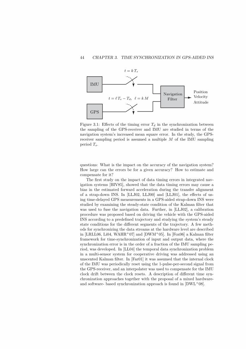
44 CHAPTER 3. TIME SYNCHRONIZATION IN GPS-AIDED INS
IMU
Navigation
GPS
Filter
Position
Velocity
Attitude
t = k Ts
t = ℓ Ts − Td, ℓ = kM
Figure 3.1: Effects of the timing error Td in the synchronization betweenthe sampling of the GPS-receiver and IMU are studied in terms of thenavigation system’s increased mean square error. In the study, the GPS-receiver sampling period is assumed a multiple M of the IMU samplingperiod Ts.
questions: What is the impact on the accuracy of the navigation system?How large can the errors be for a given accuracy? How to estimate andcompensate for it?
The first study on the impact of data timing errors in integrated nav-igation systems [BIV85], showed that the data timing errors may cause abias in the estimated forward acceleration during the transfer alignmentof a strap-down INS. In [LLJ02, LLJ00] and [LLJ01], the effects of us-ing time-delayed GPS measurements in a GPS-aided strap-down INS werestudied by examining the steady-state condition of the Kalman filter thatwas used to fuse the navigation data. Further, in [LLJ02], a calibrationprocedure was proposed based on driving the vehicle with the GPS-aidedINS according to a predefined trajectory and studying the system’s steadystate conditions for the different segments of the trajectory. A few meth-ods for synchronizing the data streams at the hardware level are describedin [LRLL06, Li04, WAHR+07] and [DWM+05]. In [Fox06] a Kalman filterframework for time-synchronization of input and output data, where thesynchronization error is in the order of a fraction of the IMU sampling pe-riod, was developed. In [LL04] the temporal data synchronization problemin a multi-sensor system for cooperative driving was addressed using anunscented Kalman filter. In [Far01] it was assumed that the internal clockof the IMU was periodically reset using the 1-pulse-per-second signal fromthe GPS-receiver, and an interpolater was used to compensate for the IMUclock drift between the clock resets. A description of different time syn-chronization approaches together with the proposal of a mixed hardware-and software- based synchronization approach is found in [DWL+08].

3.2. MSE OF THE STATE ESTIMATE 45
3.2 MSE of the State Estimate
To evaluate the effects of the time synchronization error on the performanceof the navigation system, the method that is used to fuse the sensor datamust be specified. In this study, a feedback implementation of a comple-mentary filter is used to fuse the navigation data. In other words, given alinear state space model of how the position, velocity, attitude, and sensorerrors in the mechanization of the INS develop with time, a Kalman filteris used to estimate the error state of the INS. The estimated navigationerrors are then fed back into the INS to correct its internal states. As themodel for the error plant of the INS depends on the current navigationstate, an indirect extended Kalman filter is created. Hence, to evaluatehow the timing error will affect the performance of the navigation system,the state-space model of the error plant and the extended Kalman filterrecursions must be studied.
Accordingly, a state vector xk of the form xk =[δrTk δuTk
]Twhere
δrk contains the position, velocity, attitude perturbation of the INS, andδuk, the IMU sensor errors, is introduced. Here, T denotes the transposeoperation. Subsequently, the error plant of the INS can be described by astate-space model of the form
xk+1 = Ψk xk + Gk ek (3.1)
where the state transition matrix Ψk describes how the errors develop fromone time instant to another and can be found by a perturbation analysisor linearization of the mechanized navigation equations and sensor models.For more details on how this process is carried out [FB98] can be referred.Further, the process noise gain matrix Gk describes how the measurementnoise ek from the inertial sensors affects the navigation error. As the GPSand the IMU in most cases are sampled at two different rates, the followingdown-sampling function is introduced
∆(k) =
1, k = nM, n = 1, 2, . . .0, otherwise
. (3.2)
Here, M denotes the ratio between the sampling rate of the IMU and theGPS-receiver, and is considered as an integer. If the difference betweenthe position estimates of the GPS and the INS is observed, the observationequation for the state-space model is given by
zk = Hk xk + ∆(k)wk (3.3)
where the measurement matrix Hk is defined as
Hk = ∆(k)[Iβ 0β,(α−β)]. (3.4)
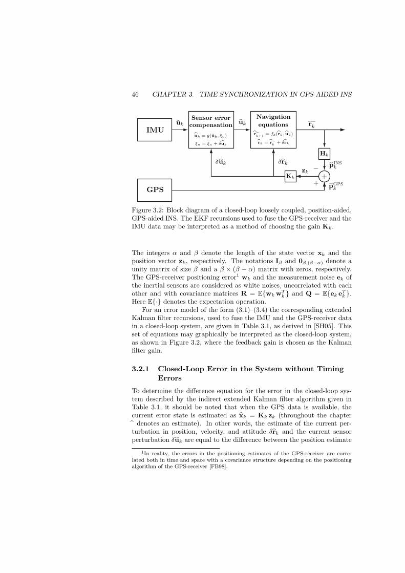
46 CHAPTER 3. TIME SYNCHRONIZATION IN GPS-AIDED INS
r−k
pINSk
pGPSk
δrk
ukuk
δukzk
+
−
r−
k+1= fd (rk, uk)
rk = r−
k+ δrk
uk = g(uk, ξu)
ξu = ξu + δuk
+
Hk
Kk
IMU
Navigationequations
GPS
Sensor errorcompensation
Figure 3.2: Block diagram of a closed-loop loosely coupled, position-aided,GPS-aided INS. The EKF recursions used to fuse the GPS-receiver and theIMU data may be interpreted as a method of choosing the gain Kk.
The integers α and β denote the length of the state vector xk and theposition vector zk, respectively. The notations Iβ and 0β,(β−α) denote aunity matrix of size β and a β × (β − α) matrix with zeros, respectively.The GPS-receiver positioning error1 wk and the measurement noise ek ofthe inertial sensors are considered as white noises, uncorrelated with eachother and with covariance matrices R = EwkwTk and Q = Eek eTk .Here E· denotes the expectation operation.
For an error model of the form (3.1)–(3.4) the corresponding extendedKalman filter recursions, used to fuse the IMU and the GPS-receiver datain a closed-loop system, are given in Table 3.1, as derived in [SH05]. Thisset of equations may graphically be interpreted as the closed-loop system,as shown in Figure 3.2, where the feedback gain is chosen as the Kalmanfilter gain.
3.2.1 Closed-Loop Error in the System without TimingErrors
To determine the difference equation for the error in the closed-loop sys-tem described by the indirect extended Kalman filter algorithm given inTable 3.1, it should be noted that when the GPS data is available, thecurrent error state is estimated as xk = Kk zk (throughout the chapter denotes an estimate). In other words, the estimate of the current per-turbation in position, velocity, and attitude δrk and the current sensorperturbation δuk are equal to the difference between the position estimate
1In reality, the errors in the positioning estimates of the GPS-receiver are corre-lated both in time and space with a covariance structure depending on the positioningalgorithm of the GPS-receiver [FB98].
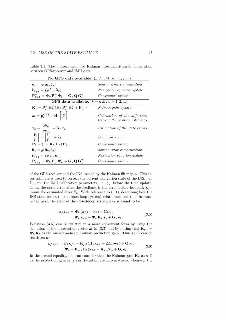
3.2. MSE OF THE STATE ESTIMATE 47
Table 3.1: The indirect extended Kalman filter algorithm for integrationbetween GPS-receiver and IMU data.
No GPS data available. (k 6= nM , n = 1, 2, ...)
uk = g(uk, ξu) Sensor error compensation
r−k+1 = fd(r−k , uk) Navigation equation update
P−k+1 = Ψk P−k ΨTk + GkQ GTk Covariance update
GPS data available. (k = nM , n = 1, 2, ...)
Kk = P−k HTk (Hk P−k HTk + R)−1 Kalman gain update
zk = pGPSk −Hk
[r−k0
]Calculation of the differencebetween the position estimates
xk =
[δrkδuk
]= Kk zk Estimation of the state errors
[rkξu
]=
[r−kξu
]+ xk Error correction
Pk = (I−KkHk) P−k Covariance update
uk = g(uk, ξu) Sensor error compensation
r−k+1 = fd(rk, uk) Navigation equation update
P−k+1 = Ψk P−k ΨTk + GkQ GTk Covariance update
of the GPS-receiver and the INS, scaled by the Kalman filter gain. This er-ror estimate is used to correct the current navigation state of the INS, i.e.,r−k , and the IMU calibration parameters, i.e., ξu, before the time update.Thus, the state error after the feedback is the error before feedback xf,kminus the estimated error xk. With reference to (3.1), describing how theINS state errors (in the open-loop system) relate from one time instanceto the next, the error of the closed-loop system xf,k is found to be
xf,k+1 = Ψk (xf,k − xk) + Gk ek
= Ψk xf,k −ΨkKk zk + Gk ek.(3.5)
Equation (3.5) can be written in a more convenient form by using thedefinition of the observation vector zk in (3.3) and by noting that Kp,k =ΨkKk is the one-step-ahead Kalman prediction gain. Thus (3.5) can berewritten as
xf,k+1 = Ψkxf,k −Kp,k(Hkxf,k + ∆(k)wk) + Gkek
= (Ψk −Kp,kHk)xf,k −Kp,kwk + Gkek.(3.6)
In the second equality, one can consider that the Kalman gain Kk as wellas the prediction gain Kp,k per definition are zero matrices, whenever the
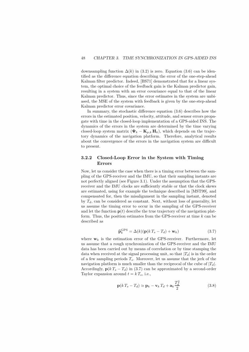
48 CHAPTER 3. TIME SYNCHRONIZATION IN GPS-AIDED INS
downsampling function ∆(k) in (3.2) is zero. Equation (3.6) can be iden-tified as the difference equation describing the error of the one-step-aheadKalman filter predictor. Indeed, [BS71] demonstrated that for a linear sys-tem, the optimal choice of the feedback gain is the Kalman predictor gain,resulting in a system with an error covariance equal to that of the linearKalman predictor. Thus, since the error estimates in the system are unbi-ased, the MSE of the system with feedback is given by the one-step-aheadKalman predictor error covariance.
In summary, the stochastic difference equation (3.6) describes how theerrors in the estimated position, velocity, attitude, and sensor errors propa-gate with time in the closed-loop implementation of a GPS-aided INS. Thedynamics of the errors in the system are determined by the time varyingclosed-loop system matrix (Ψk −Kp,kHk), which depends on the trajec-tory dynamics of the navigation platform. Therefore, analytical resultsabout the convergence of the errors in the navigation system are difficultto present.
3.2.2 Closed-Loop Error in the System with TimingErrors
Now, let us consider the case when there is a timing error between the sam-pling of the GPS-receiver and the IMU, so that their sampling instants arenot perfectly aligned (see Figure 3.1). Under the assumption that the GPS-receiver and the IMU clocks are sufficiently stable or that the clock skewsare estimated, using for example the technique described in [MST99], andcompensated for, then the misalignment in the sampling instant, denotedby Td, can be considered as constant. Next, without loss of generality, letus assume the timing error to occur in the sampling of the GPS-receiverand let the function p(t) describe the true trajectory of the navigation plat-form. Thus, the position estimates from the GPS-receiver at time k can bedescribed as
pGPSk = ∆(k)(p(k Ts − Td) + wk) (3.7)
where wk is the estimation error of the GPS-receiver. Furthermore, letus assume that a rough synchronization of the GPS-receiver and the IMUdata has been carried out by means of correlation or by time stamping thedata when received at the signal processing unit, so that |Td| is in the orderof a few sampling periods Ts. Moreover, let us assume that the jerk of thenavigation platform is much smaller than the reciprocal of the cube of |Td|.Accordingly, p(k Ts − Td) in (3.7) can be approximated by a second-orderTaylor expansion around t = k Ts, i.e.,
p(k Ts − Td) ≃ pk − vk Td + akT 2d
2(3.8)

3.2. MSE OF THE STATE ESTIMATE 49
where pk, vk, and ak denote the navigation platform position, velocity, andacceleration at sampling instance k, respectively. The symbol ≃ denotesan equality where only the significant terms are retained (i.e., third andhigher-order terms in Td are neglected). By inserting (3.8) into (3.7), weget
pGPSk ≃ ∆(k)
(pk − vk Td + ak
T 2d
2+ wk
). (3.9)
Thus, the true observation zak of the system, which is fed back into theclosed-loop system, can be described as
zak = ∆(k)(pGPSk − pINS
k )
≃ ∆(k)(pk − vk Td + akT 2d
2+ wk − pINS
k ).(3.10)
Here pINSk is the position estimate from the INS at time k. Subsequently,
identifying that Hk xf,k = ∆(k)(pk − pINSk ) and substituting it into (3.10)
yields the following description of the true observation for the system witha timing error
zak ≃ ∆(k)(Hk xf,k + wk + dk). (3.11)
In (3.11), the position error bias vector dk is introduced as
dk = −vk Td + akT 2d
2. (3.12)
By comparing (3.11) and (3.3) it can be clearly noted that the actual obser-vation contains not only the position error and the GPS-receiver estimationerror wk, but also a bias term dk that depends on the timing error Td andthe dynamics of the navigation system. By substituting zk with zak in (3.5)and inserting (3.11) into this, along with a slight misusage of the subscriptnotation, the following difference equation for the error state in the closed-loop navigation system with timing errors can be obtained
xfd,k+1 = Ψk xfd,k −Kp,k zak + Gk ek
= Ψk xfd,k −Kp,k
(∆(k)(Hk xfd,k
+ wk + dk))
+ Gk ek.
(3.13)
Here the subscript (·)fd is used to denote the difference from the stateerrors in the closed-loop system without timing error. By examining therecursions in Table 3.1, it is clear that the Kalman filter gain Kk and
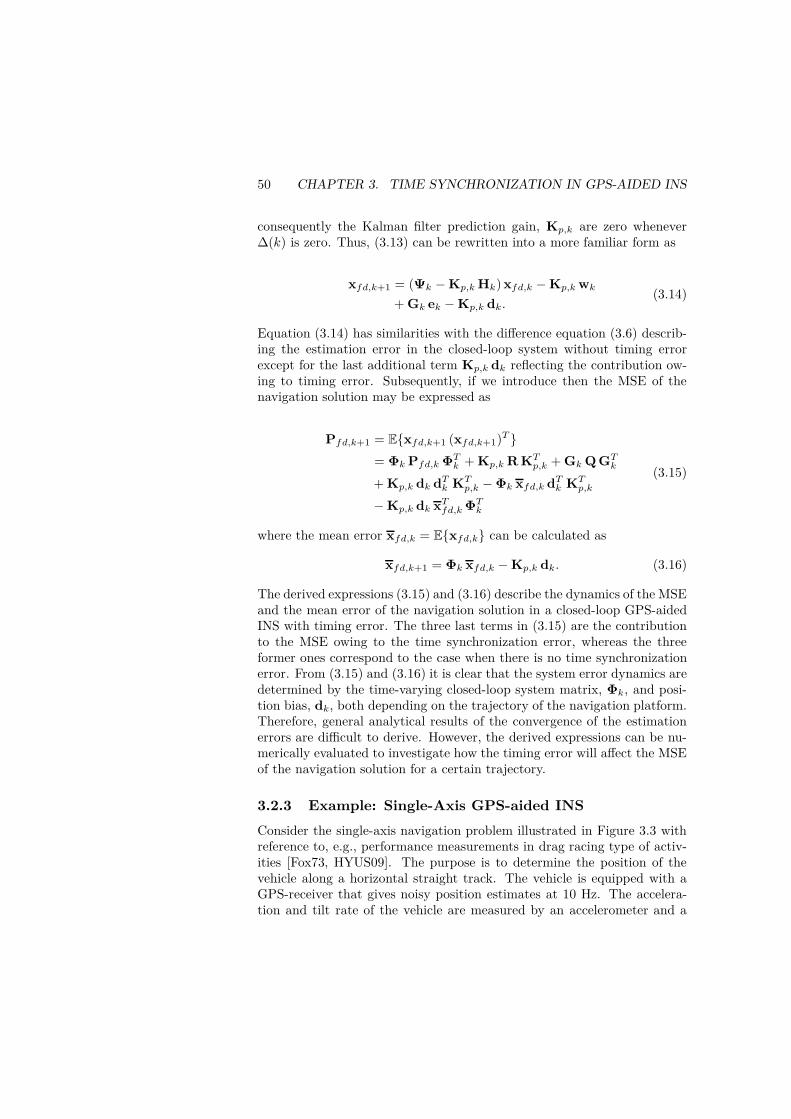
50 CHAPTER 3. TIME SYNCHRONIZATION IN GPS-AIDED INS
consequently the Kalman filter prediction gain, Kp,k are zero whenever∆(k) is zero. Thus, (3.13) can be rewritten into a more familiar form as
xfd,k+1 = (Ψk −Kp,kHk) xfd,k −Kp,kwk
+ Gk ek −Kp,k dk.(3.14)
Equation (3.14) has similarities with the difference equation (3.6) describ-ing the estimation error in the closed-loop system without timing errorexcept for the last additional term Kp,k dk reflecting the contribution ow-ing to timing error. Subsequently, if we introduce then the MSE of thenavigation solution may be expressed as
Pfd,k+1 = Exfd,k+1 (xfd,k+1)T = ΦkPfd,kΦTk + Kp,kR KTp,k + GkQ GTk
+ Kp,k dk dTk KTp,k −Φk xfd,k dTk KTp,k
−Kp,k dk xTfd,kΦTk
(3.15)
where the mean error xfd,k = Exfd,k can be calculated as
xfd,k+1 = Φk xfd,k −Kp,k dk. (3.16)
The derived expressions (3.15) and (3.16) describe the dynamics of the MSEand the mean error of the navigation solution in a closed-loop GPS-aidedINS with timing error. The three last terms in (3.15) are the contributionto the MSE owing to the time synchronization error, whereas the threeformer ones correspond to the case when there is no time synchronizationerror. From (3.15) and (3.16) it is clear that the system error dynamics aredetermined by the time-varying closed-loop system matrix, Φk, and posi-tion bias, dk, both depending on the trajectory of the navigation platform.Therefore, general analytical results of the convergence of the estimationerrors are difficult to derive. However, the derived expressions can be nu-merically evaluated to investigate how the timing error will affect the MSEof the navigation solution for a certain trajectory.
3.2.3 Example: Single-Axis GPS-aided INS
Consider the single-axis navigation problem illustrated in Figure 3.3 withreference to, e.g., performance measurements in drag racing type of activ-ities [Fox73, HYUS09]. The purpose is to determine the position of thevehicle along a horizontal straight track. The vehicle is equipped with aGPS-receiver that gives noisy position estimates at 10 Hz. The accelera-tion and tilt rate of the vehicle are measured by an accelerometer and a

3.2. MSE OF THE STATE ESTIMATE 51
accelerationa(t)
ω(t)
gravity vectorgravity vector
accelerometersensitivity axis
Figure 3.3: Example of a single-axis GPS-aided INS system.
gyroscope, respectively. When the vehicle accelerates it will start to tiltand the accelerometer will not only sense the forward acceleration but alsothe gravitational acceleration. If we assume the gravity vector to have themagnitude, g, then the relationship between the acceleration and angularrate of the vehicle and its tilt angle, velocity, and position can be describedby the following set of differential equations:
p(t) = v(t) (3.17)
v(t) = s(t)/ cos(φ(t)) − g tan(φ(t)) (3.18)
φ(t) = ω(t) (3.19)
Here, p(t), v(t), s(t), φ(t), and ω(t) denote the position, velocity, specificforce, tilt, and angular rate of the vehicle, respectively. These equationsare referred to as the navigation equations used in the INS to calculatethe position, velocity, and tilt from the measured specific force and angu-lar rates. By introducing the state vector rc =
[p(t) v(t) φ(t)
]Tand
input vector uc =[s(t) ω(t)
]T, the continuous time navigation equa-
tions (3.17)–(3.19) may be written as rc = fc(rc,uc). Assuming that thereis a bias, δωc, and noise, ec,2, in the gyroscope measurements, and thatthe specific force measurements are only disturbed by some noise ec,1, themeasured output from the accelerometer and gyroscope can be described assc = sc+ ec,1 and ωc = ωc− δ ωc+ ec,2, respectively. Using these measure-ments as the input to the INS results in an error in the calculated position,velocity, and tilt. A linear model describing how the errors develop withtime may be obtained by linearizing the navigation equations around thetrue trajectory, i.e.,
˙rc = rc − δrc = fc(rc, uc)
≃ fc(rc,uc)−∂fc(r,u)
∂r
∣∣∣∣r=rc
δrc +∂fc(r,u)
∂sc
∣∣∣∣u=uc
ec,1
− ∂fc(r,u)
∂ωc
∣∣∣∣u=uc
(δωc − ec,2).
(3.20)
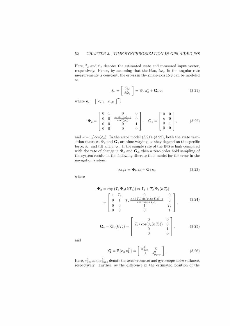
52 CHAPTER 3. TIME SYNCHRONIZATION IN GPS-AIDED INS
Here, rc and uc denotes the estimated state and measured input vector,respectively. Hence, by assuming that the bias, δωc, in the angular ratemeasurements is constant, the errors in the single-axis INS can be modeledas
xc =
[δrcδωc
]= Ψc xec + Gc ec (3.21)
where ec =[ec,1 ec,2
]T,
Ψc =
0 1 0 0
0 0 sc sin(φc)−gcos2(φc)
0
0 0 0 10 0 0 0
, Gc =
0 0κ 00 10 0
, (3.22)
and κ = 1/ cos(φc). In the error model (3.21)–(3.22), both the state tran-sition matrices Ψc and Gc are time varying, as they depend on the specificforce, sc, and tilt angle, φc. If the sample rate of the INS is high comparedwith the rate of change in Ψc and Gc, then a zero-order hold sampling ofthe system results in the following discrete time model for the error in thenavigation system.
xk+1 = Ψk zk + Gk ek (3.23)
where
Ψk = exp (TsΨc(k Ts)) ≈ I4 + TsΨc(k Ts)
=
1 Ts 0 0
0 1 Tssc(k Ts) sin(φc(k Ts))−g
cos2(φc(k Ts)) 0
0 0 1 Ts0 0 0 1
,(3.24)
Gk = Gc(k Ts) =
0 0Ts/ cos(φc(k Ts)) 0
0 10 0
, (3.25)
and
Q = Eek eTk =
[σ2acc 00 σ2
gyro
]. (3.26)
Here, σ2acc and σ2
gyro denote the accelerometer and gyroscope noise variance,respectively. Further, as the difference in the estimated position of the

3.2. MSE OF THE STATE ESTIMATE 53
0 100 200 300 400 5000
5000
10000
15000
0 100 200 300 400 5000
20
0 100 200 300 400 500
−5
0
5
Position
[m]
Velocity
[m/s
]
Tilt
[]
Time [s]
Figure 3.4: Trajectory used in the single-axis GPS-aided INS example.
GPS-receiver and the INS is observed, the observation equation for theerror model becomes
zk = Hk xk + ∆(k) wk (3.27)
whereHk = ∆(k)
[1 01,3
](3.28)
and
R = EwkwTk = σ2gps. (3.29)
Having derived the state-space model for the error plant in the singleaxis INS system, which has the same structure as the error model in (3.1)–(3.4), the results in (3.15)–(3.16) can, given the vehicle trajectory, be ap-plied to evaluate how the time synchronization error affects the accuracyof the integrated navigation system. For example, consider the vehicletrajectory described in Figure 3.4, then the expected performance (i.e.,the performance predicted by evaluating (3.15)–(3.16) given the system er-ror model and vehicle trajectory) in terms of the root mean square error(RMSE) in the navigation solution of the integrated navigation system withan inherent time synchronization error of 50 ms is shown in Figure 3.6. Inthe example, the system parameters are those given in Table 3.2. A MonteCarlo (MC) simulation of the single-axis navigation example was also con-ducted to illustrate the error model in (3.15)–(3.16). The MC simulationcalculated RMSE, indicated in red in Figure 3.6, demonstrate good agree-ment with those calculated from the error model.
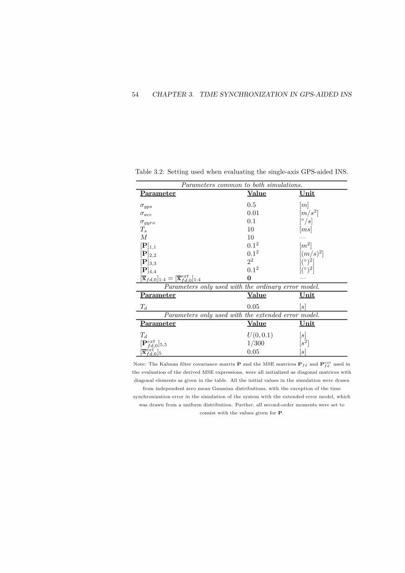
54 CHAPTER 3. TIME SYNCHRONIZATION IN GPS-AIDED INS
Table 3.2: Setting used when evaluating the single-axis GPS-aided INS.
Parameters common to both simulations.Parameter Value Unit
σgps 0.5 [m]σacc 0.01 [m/s2]σgyro 0.1 [/s]Ts 10 [ms]M 10 —[P]1,1 0.12 [m2][P]2,2 0.12 [(m/s)2][P]3,3 22 [()2][P]4,4 0.12 [()2][xfd,0]1:4 = [xextfd,0]1:4 0 —
Parameters only used with the ordinary error model.Parameter Value Unit
Td 0.05 [s]Parameters only used with the extended error model.
Parameter Value Unit
Td U(0, 0.1) [s][Pextfd,0]5,5 1/300 [s2]
[xextfd,0]5 0.05 [s]
Note: The Kalman filter covariance matrix P and the MSE matrices Pfd and Pextfd used in
the evaluation of the derived MSE expressions, were all initialized as diagonal matrices with
diagonal elements as given in the table. All the initial values in the simulation were drawn
from independent zero mean Gaussian distributions, with the exception of the time
synchronization error in the simulation of the system with the extended error model, which
was drawn from a uniform distribution. Further, all second-order moments were set to
consist with the values given for P.

3.3. ESTIMATING AND REMOVING THE TIMING ERROR 55
3.3 Estimating and Removing the Timing Error
The dependence between the timing error Td and the bias in the observedposition difference zak, see (3.10), can be exploited to calculate an estimateof the timing error. A description of how this can be done, using theclosed-loop system structure and extended Kalman filtering described inSection 3.2, is given next; a model for the MSE of the state estimate of thecorresponding system is also derived.
To use the closed-loop system structure employed in Section 3.2 to alsoestimate and compensate for the timing error, two things must be done.First, the state space model used in the extended Kalman filter must beextended to also included the timing error. Secondly, a method for time-shifting the IMU measurements, in accordance with estimated timing errormust be implemented.
3.3.1 Estimating the Timing Error
To find the extended error model, let Td,k be the estimate of the timingerror at time instant k, which is used to control a variable delay filtersynchronizing the GPS-receiver and the IMU data streams, as illustratedin Figure 3.5. (Note that the sample index k from now on refers to the timeinstant t = k Ts− Td,k.) Further, let δTd,k = Td− Td,k be the correspondingestimation error. The error propagation in the open-loop system systemcan then be described by the extended error model
xextk+1 = Ψextk xextk + Gextk ek, (3.30)
where xextk = [xTk δTd,k]T is the extended error state vector and
Ψextk =
[Ψk 0α,101,α 1
]and Gextk =
[Gk0
]. (3.31)
The structure of Ψextk and Gextk are due to the fact that the timing errorwas assumed constant. Next, to find the measurement matrix for the ex-tended error model, Hextk , let us once again do a second-order Taylor seriesexpansion of the GPS-receiver position estimate as in (3.9), but this timearound k Ts − Td,k. That, is
pGPSk = ∆(k)
(p(k Ts − Td) + wk
)
= ∆(k)(
p(k Ts − Td,k − δTd,k) + wk
)
≃ ∆(k)(
pk − vkδTd,k + akδT 2d,k
2+ wk
).
(3.32)
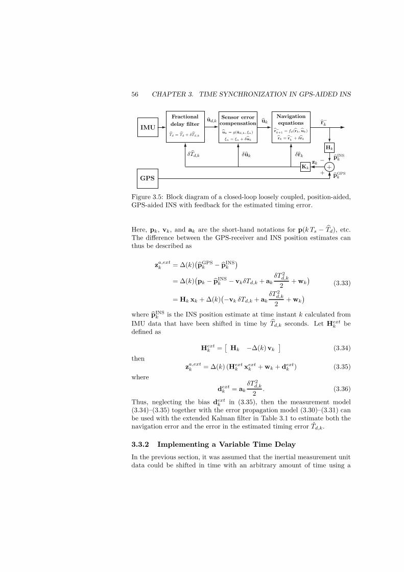
56 CHAPTER 3. TIME SYNCHRONIZATION IN GPS-AIDED INS
r−k
pINSk
pGPSk
δrk
uk
δukzk
+
−
r−
k+1= fd (rk, uk)
rk = r−
k+ δrk
uk = g(ud,k, ξu)
ξu = ξu + δuk
Fractional
delay filter
+
Hk
Kk
IMU
Navigationequations
GPS
Sensor errorcompensation
Td = Td + δTd,k
δTd,k
ud,k
Figure 3.5: Block diagram of a closed-loop loosely coupled, position-aided,GPS-aided INS with feedback for the estimated timing error.
Here, pk, vk, and ak are the short-hand notations for p(k Ts − Td), etc.The difference between the GPS-receiver and INS position estimates canthus be described as
za,extk = ∆(k)(pGPSk − pINS
k
)
= ∆(k)(pk − pINS
k − vkδTd,k + akδT 2d,k
2+ wk
)
= Hk xk + ∆(k)(−vk δTd,k + ak
δT 2d,k
2+ wk
)(3.33)
where pINSk is the INS position estimate at time instant k calculated from
IMU data that have been shifted in time by Td,k seconds. Let Hextk bedefined as
Hextk =[
Hk −∆(k) vk]
(3.34)
thenza,extk = ∆(k) (Hextk xextk + wk + dextk ) (3.35)
where
dextk = akδT 2d,k
2. (3.36)
Thus, neglecting the bias dextk in (3.35), then the measurement model(3.34)–(3.35) together with the error propagation model (3.30)–(3.31) canbe used with the extended Kalman filter in Table 3.1 to estimate both thenavigation error and the error in the estimated timing error Td,k.
3.3.2 Implementing a Variable Time Delay
In the previous section, it was assumed that the inertial measurement unitdata could be shifted in time with an arbitrary amount of time using a

3.3. ESTIMATING AND REMOVING THE TIMING ERROR 57
0 20 40 60 80 1000
1
2
0 20 40 60 80 1000
0.2
0.4
0 20 40 60 80 1000
0.02
0.04
RMSE of the position estimate.
RM
SE[m
]
RMSE of the velocity estimate.
RM
SE[m/s]
RMSE of the tilt estimate.
RM
SE[]
Time [s]
Figure 3.6: RMSE of the estimated position, velocity, and tilt for a timesynchronization error of 50 ms. (a) No timing error – dashed black line withtriangles, (b) MSE model – blue line with squares, and (c) MC simulation– red line with circles.
variable delay. However, in reality the IMU data are sampled at certaintime instances. To have a continuously variable time-shift D = Td/Ts,an adjustable interpolator or fractional delay filter must be used. Oneof the most commonly used techniques for fractional delay filter design isthe Lagrange interpolation, in which the filter coefficients of the fractionaldelay FIR filter is calculated as [LVKL96]
h(n) =
N∏
k=0k 6=n
D − kn− k forn = 0, 1, 2, ..., N. (3.37)
Here N is the order of the filter and D ∈ [(N − 1)/2, (N + 1)/2] is thedesired delay. If a delay larger than D = (N+1)/2 is required, this may besolved by adding an appropriate number of unit-delays before the fractionaldelay FIR filter.
3.3.3 MSE of the State Estimate in the Extended System
A model for the MSE and mean error of the state vector estimate in thesystem that also estimates the timing error can be found by substitutingzk in (3.5) with za,extk . Thus, the estimation error in the extended systemdevelops with time as
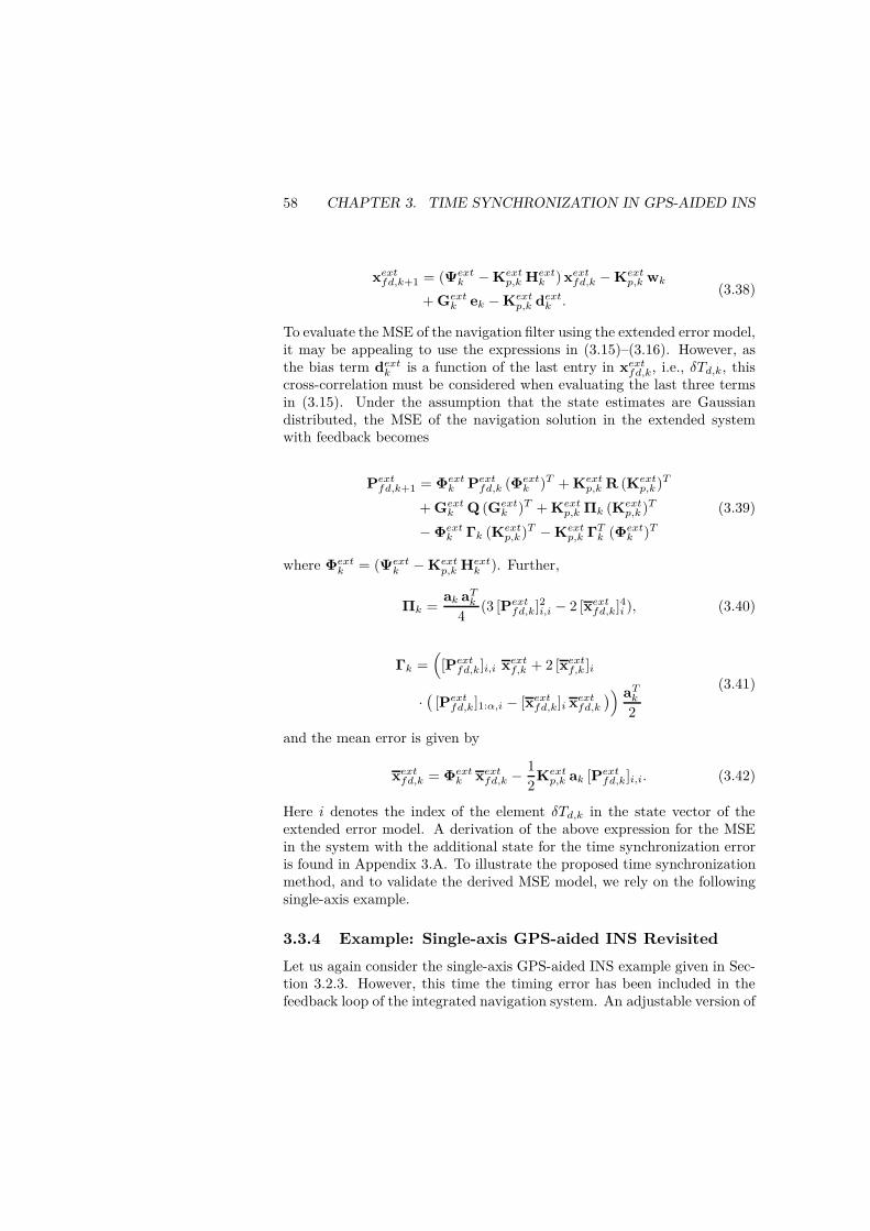
58 CHAPTER 3. TIME SYNCHRONIZATION IN GPS-AIDED INS
xextfd,k+1 = (Ψextk −Kextp,k Hextk ) xextfd,k −Kextp,k wk
+ Gextk ek −Kextp,k dextk .(3.38)
To evaluate the MSE of the navigation filter using the extended error model,it may be appealing to use the expressions in (3.15)–(3.16). However, asthe bias term dextk is a function of the last entry in xextfd,k, i.e., δTd,k, thiscross-correlation must be considered when evaluating the last three termsin (3.15). Under the assumption that the state estimates are Gaussiandistributed, the MSE of the navigation solution in the extended systemwith feedback becomes
Pextfd,k+1 = Φextk Pextfd,k (Φextk )T + Kextp,k R (Kextp,k)T
+ Gextk Q (Gextk )T + Kextp,k Πk (Kextp,k )T
−Φextk Γk (Kextp,k)T −Kextp,k ΓTk (Φextk )T
(3.39)
where Φextk = (Ψextk −Kextp,k Hextk ). Further,
Πk =ak aTk
4(3 [Pextfd,k]
2i,i − 2 [xextfd,k]
4i ), (3.40)
Γk =(
[Pextfd,k]i,i xextf,k + 2 [xextf,k ]i
·(
[Pextfd,k]1:α,i − [xextfd,k]i xextfd,k
)) aTk2
(3.41)
and the mean error is given by
xextfd,k = Φextk xextfd,k −1
2Kextp,k ak [Pextfd,k]i,i. (3.42)
Here i denotes the index of the element δTd,k in the state vector of theextended error model. A derivation of the above expression for the MSEin the system with the additional state for the time synchronization erroris found in Appendix 3.A. To illustrate the proposed time synchronizationmethod, and to validate the derived MSE model, we rely on the followingsingle-axis example.
3.3.4 Example: Single-axis GPS-aided INS Revisited
Let us again consider the single-axis GPS-aided INS example given in Sec-tion 3.2.3. However, this time the timing error has been included in thefeedback loop of the integrated navigation system. An adjustable version of
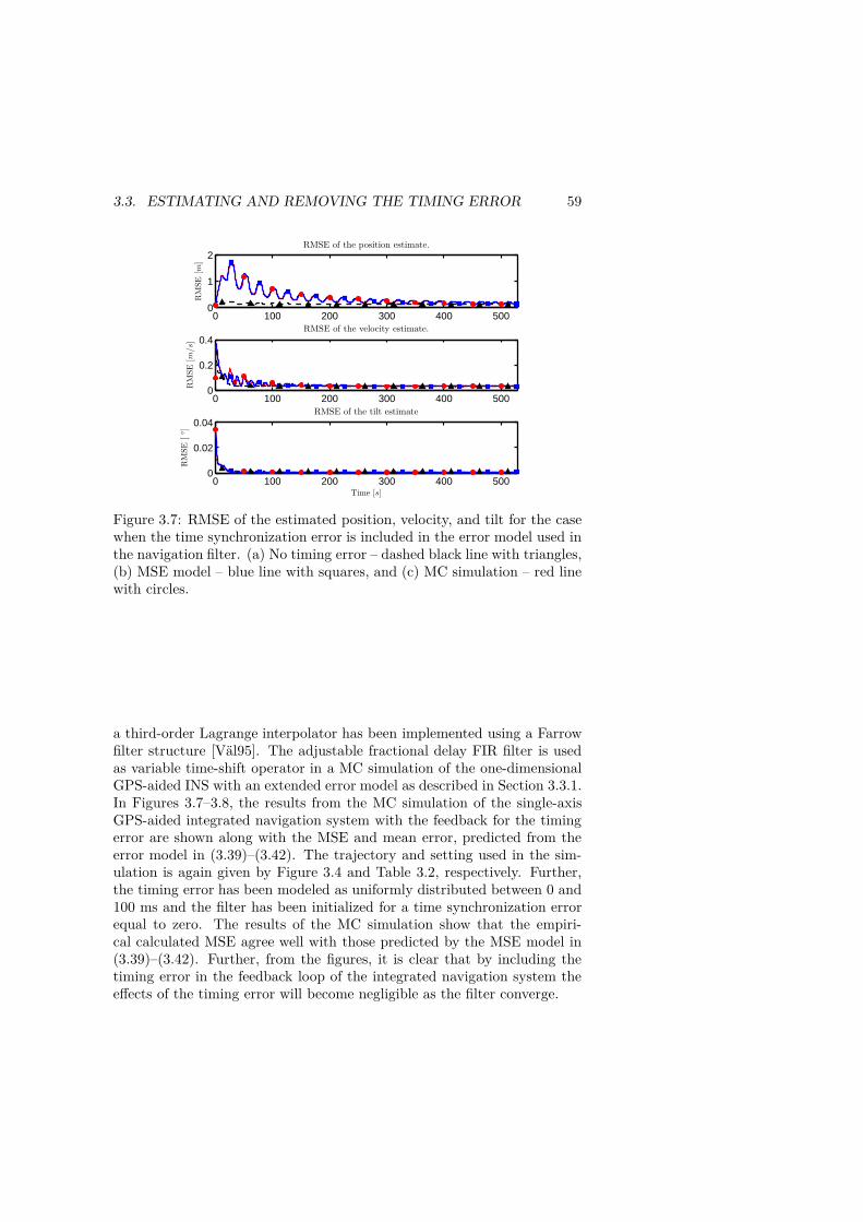
3.3. ESTIMATING AND REMOVING THE TIMING ERROR 59
0 100 200 300 400 5000
1
2
0 100 200 300 400 5000
0.2
0.4
0 100 200 300 400 5000
0.02
0.04
RMSE of the position estimate.
RM
SE[m
]
RMSE of the velocity estimate.
RM
SE[m/s]
RMSE of the tilt estimate
RM
SE[]
Time [s]
Figure 3.7: RMSE of the estimated position, velocity, and tilt for the casewhen the time synchronization error is included in the error model used inthe navigation filter. (a) No timing error – dashed black line with triangles,(b) MSE model – blue line with squares, and (c) MC simulation – red linewith circles.
a third-order Lagrange interpolator has been implemented using a Farrowfilter structure [Väl95]. The adjustable fractional delay FIR filter is usedas variable time-shift operator in a MC simulation of the one-dimensionalGPS-aided INS with an extended error model as described in Section 3.3.1.In Figures 3.7–3.8, the results from the MC simulation of the single-axisGPS-aided integrated navigation system with the feedback for the timingerror are shown along with the MSE and mean error, predicted from theerror model in (3.39)–(3.42). The trajectory and setting used in the sim-ulation is again given by Figure 3.4 and Table 3.2, respectively. Further,the timing error has been modeled as uniformly distributed between 0 and100 ms and the filter has been initialized for a time synchronization errorequal to zero. The results of the MC simulation show that the empiri-cal calculated MSE agree well with those predicted by the MSE model in(3.39)–(3.42). Further, from the figures, it is clear that by including thetiming error in the feedback loop of the integrated navigation system theeffects of the timing error will become negligible as the filter converge.

60 CHAPTER 3. TIME SYNCHRONIZATION IN GPS-AIDED INS
0 100 200 300 400 5000
0.02
0.04
0.06
0 100 200 300 400 5000
0.02
0.04
0.06
RMSE of the time synchronization error estimate.
Mean error of time synchronization error estimate.
Time [s]
Time [s]
RM
SE[s
]M
ean
[s]
Figure 3.8: RMSE and mean error of the time synchronization error esti-mate. (a) MSE an mean error model – blue line (squares), (b) MC simu-lation – red line (circles).
3.4 Time Synchronization in GPS-aided INS
To further illustrate the usefulness of the fractional delay filter time syn-chronization approach, it was implemented as a part of the Matlab softwaredeveloped in-house for integrating GPS and IMU data. The synchroniza-tion approach was then tested on both simulated and real-world data, intowhich intentional time synchronization errors were included. The soft-ware was developed targeting simulations and tests of ultra low-cost GPS-aided INS applications, such as consumer electronics in-car navigation ap-plications. (For more details on the PC-based navigation platform, referto [SSH06].) The integration software was designed for navigation in thetangent plane (in daily life often referred to as north, east, and down), andto be used with low-cost micro-electromechanical systems (MEMS) inertialsensors. Thus, parameters such as craft rates, gravity variations, the earthrotation rate, etc., can be neglected. For this type of low-cost applica-tions, where the above-stated assumptions can be applied, an error modelas given in Appendix 3.B is applicable [WV07].
3.4.1 Simulated Data
In Figure 3.9, the trajectory used in the MC simulations and evaluation ofthe derived MSE expression of the GPS-aided INS is shown. The results ofthe MC simulation along with the values predicted by the MSE models are

3.4. TIME SYNCHRONIZATION IN GPS-AIDED INS 61
−60 −40 −20 0 20 40 60 80 100 120−250
−200
−150
−100
−50
0
50Simulation trajectory
East [m]
Nor
th[m
]
Figure 3.9: Trajectory used in the MC simulation of the GPS-aided INSand the evaluation of the covariance expressions.
shown in Figures 3.10-3.14. In Table 3.3, the setting used in the simulationsis summarized. Figures 3.10–3.11 illustrate the case when the timing erroris not included in the system model. It can be observed that there is a goodagreement between the MSEs and mean errors predicted by the model andthose calculated from the MC simulation. In Figure 3.11, the bias in theforward acceleration owing to the timing error can be observed. When thetiming error is included in the model (see Figures 3.12–3.14), the derivedMSE expression do not perfectly capture the transient behavior of the inte-gration filter. This is probably owing to the extra nonlinearity introducedby the time shifting of the IMU data using the fractional delay filter, whichis not properly captured by the MSE expressions. However, as the filterconverges the agreement between the model predicted MSE and those cal-culated from the MC simulation improves, and it is clearly evident that theeffects of the timing error are removed. Moreover, from Figure 3.13 it isobvious that the bias in the forward acceleration is substantially reduced.
3.4.2 Real-world Data
Real-world data was collected using a 100 Hz GPS-receiver and data logger(VBOX III) together with an additional MEMS IMU, all from Racelogic. InFigure 3.15, the trajectory of the vehicle is shown. The test was conductedin a parking lot, outside Stockholm, Sweden, under the following conditions:clear sky view with no large surrounding obstacles blocking the satellitesignals and with 8–9 satellites in view during the entire run. The GPS
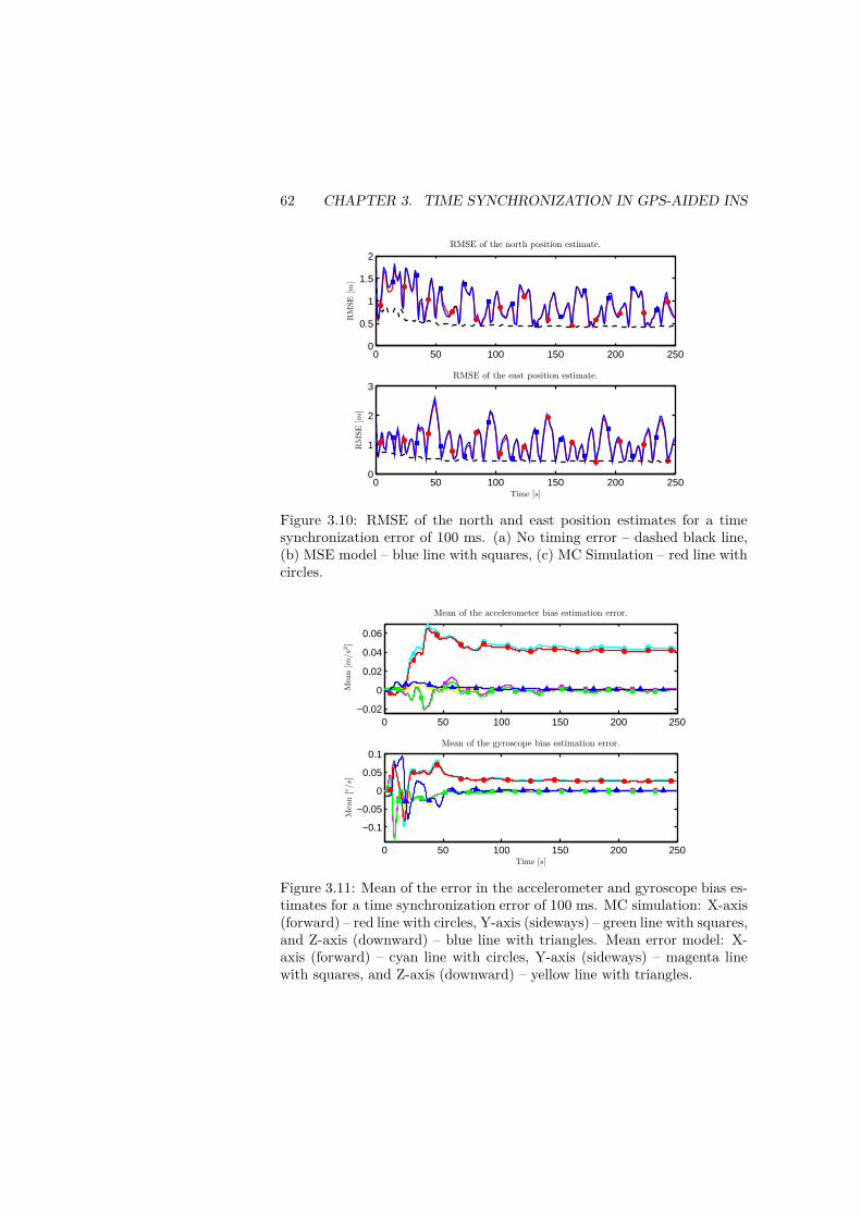
62 CHAPTER 3. TIME SYNCHRONIZATION IN GPS-AIDED INS
0 50 100 150 200 2500
0.5
1
1.5
2
0 50 100 150 200 2500
1
2
3
RMSE of the north position estimate.
RMSE of the east position estimate.
RM
SE[m
]R
MSE
[m]
Time [s]
Figure 3.10: RMSE of the north and east position estimates for a timesynchronization error of 100 ms. (a) No timing error – dashed black line,(b) MSE model – blue line with squares, (c) MC Simulation – red line withcircles.
0 50 100 150 200 250−0.02
0
0.02
0.04
0.06
0 50 100 150 200 250
−0.1
−0.05
0
0.05
0.1
Mean of the accelerometer bias estimation error.
Mean of the gyroscope bias estimation error.
Mea
n[m/s2
]M
ean
[/s]
Time [s]
Figure 3.11: Mean of the error in the accelerometer and gyroscope bias es-timates for a time synchronization error of 100 ms. MC simulation: X-axis(forward) – red line with circles, Y-axis (sideways) – green line with squares,and Z-axis (downward) – blue line with triangles. Mean error model: X-axis (forward) – cyan line with circles, Y-axis (sideways) – magenta linewith squares, and Z-axis (downward) – yellow line with triangles.
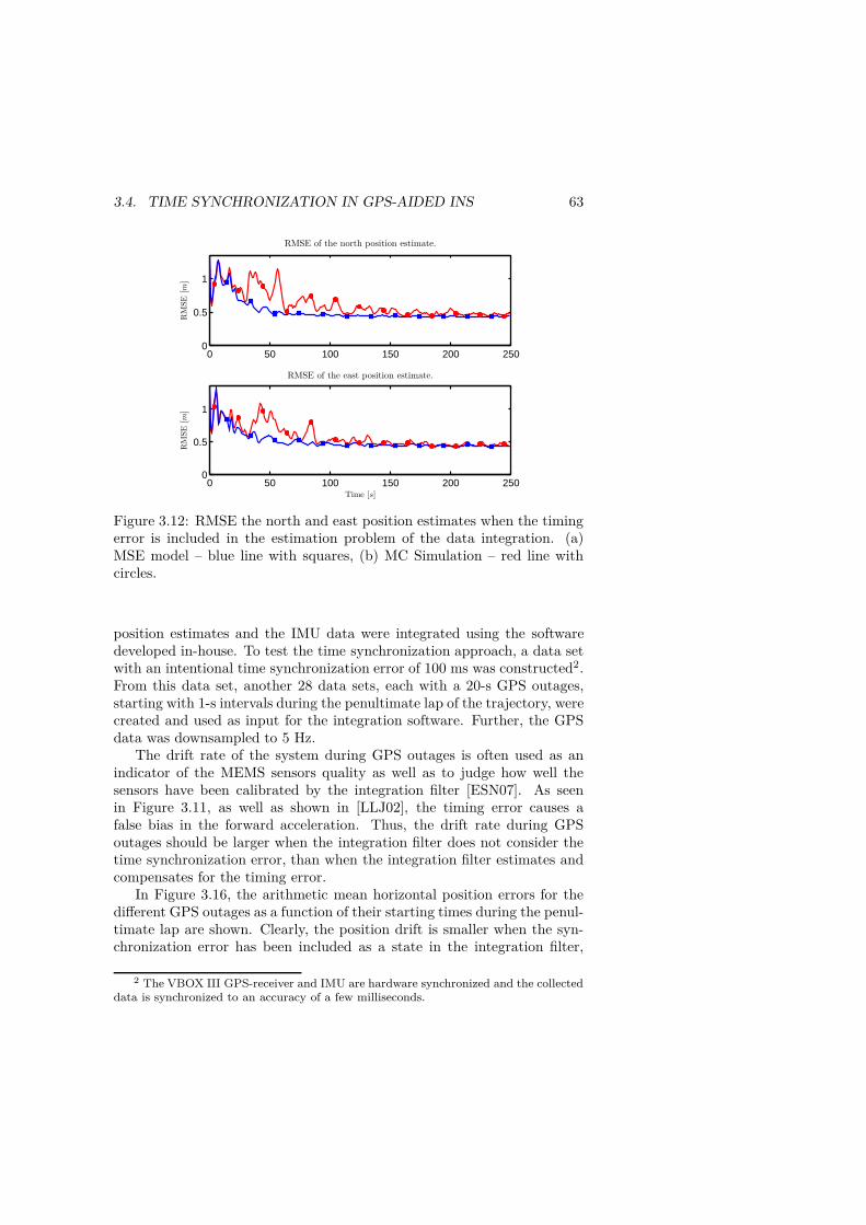
3.4. TIME SYNCHRONIZATION IN GPS-AIDED INS 63
0 50 100 150 200 2500
0.5
1
0 50 100 150 200 2500
0.5
1
RMSE of the north position estimate.
RMSE of the east position estimate.
RM
SE[m
]R
MSE
[m]
Time [s]
Figure 3.12: RMSE the north and east position estimates when the timingerror is included in the estimation problem of the data integration. (a)MSE model – blue line with squares, (b) MC Simulation – red line withcircles.
position estimates and the IMU data were integrated using the softwaredeveloped in-house. To test the time synchronization approach, a data setwith an intentional time synchronization error of 100 ms was constructed2.From this data set, another 28 data sets, each with a 20-s GPS outages,starting with 1-s intervals during the penultimate lap of the trajectory, werecreated and used as input for the integration software. Further, the GPSdata was downsampled to 5 Hz.
The drift rate of the system during GPS outages is often used as anindicator of the MEMS sensors quality as well as to judge how well thesensors have been calibrated by the integration filter [ESN07]. As seenin Figure 3.11, as well as shown in [LLJ02], the timing error causes afalse bias in the forward acceleration. Thus, the drift rate during GPSoutages should be larger when the integration filter does not consider thetime synchronization error, than when the integration filter estimates andcompensates for the timing error.
In Figure 3.16, the arithmetic mean horizontal position errors for thedifferent GPS outages as a function of their starting times during the penul-timate lap are shown. Clearly, the position drift is smaller when the syn-chronization error has been included as a state in the integration filter,
2 The VBOX III GPS-receiver and IMU are hardware synchronized and the collecteddata is synchronized to an accuracy of a few milliseconds.
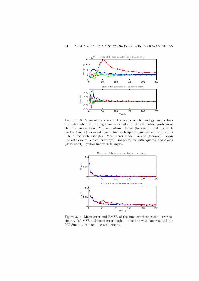
64 CHAPTER 3. TIME SYNCHRONIZATION IN GPS-AIDED INS
0 50 100 150 200 250−5
0
5
10
15x 10
−3
0 50 100 150 200 250−0.04
−0.02
0
0.02
0.04
Mean of the accelerometer bias estimation error.
Mean of the gyroscope bias estimation error.
Mea
n[m/s2
]
Mea
n[/s]
Time [s]
Figure 3.13: Mean of the error in the accelerometer and gyroscope biasestimates when the timing error is included in the estimation problem ofthe data integration. MC simulation: X-axis (forward) – red line withcircles, Y-axis (sideways) – green line with squares, and Z-axis (downward)– blue line with triangles. Mean error model: X-axis (forward) – cyanline with circles, Y-axis (sideways) – magenta line with squares, and Z-axis(downward) – yellow line with triangles.
0 50 100 150 200 2500
0.05
0.1
0 50 100 150 200 2500
0.05
0.1
Mean error of the time synchronization error estimate.
RMSE of time synchronization error estimate.
Mea
n[s
]R
MSE
[s]
Time [s]
Figure 3.14: Mean error and RMSE of the time synchronization error es-timate. (a) MSE and mean error model – blue line with squares, and (b)MC Simulation – red line with circles.
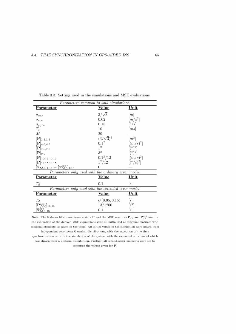
3.4. TIME SYNCHRONIZATION IN GPS-AIDED INS 65
Table 3.3: Setting used in the simulations and MSE evaluations.
Parameters common to both simulations.Parameter Value Unit
σgps 3/√
3 [m]σacc 0.02 [m/s2]σgyro 0.15 [/s]Ts 10 [ms]M 20 —[P]1:3,1:3 (3/
√3)2 [m2]
[P]4:6,4:6 0.12 [(m/s)2][P]7:8,7:8 12 [()2][P]9,9 32 [()2][P]10:12,10:12 0.12/12 [(m/s)2][P]13:15,13:15 12/12 [(/s)2][xfd,0]1:15 = [xextfd,0]1:15 0 —
Parameters only used with the ordinary error model.Parameter Value Unit
Td 0.1 [s]Parameters only used with the extended error model.
Parameter Value Unit
Td U(0.05, 0.15) [s][Pextfd,0]16,16 13/1200 [s2]
[xextfd,0]16 0.1 [s]
Note: The Kalman filter covariance matrix P and the MSE matrices Pfd and Pextfd used in
the evaluation of the derived MSE expressions were all initialized as diagonal matrices with
diagonal elements, as given in the table. All initial values in the simulation were drawn from
independent zero-mean Gaussian distributions, with the exception of the time
synchronization error in the simulation of the system with the extended error model which
was drawn from a uniform distribution. Further, all second-order moments were set to
comprise the values given for P.
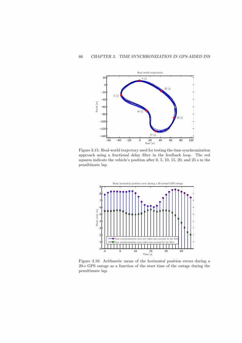
66 CHAPTER 3. TIME SYNCHRONIZATION IN GPS-AIDED INS
−60 −40 −20 0 20 40 60 80 100
−140
−120
−100
−80
−60
−40
−20
0
20
Real world trajectories
Nor
th[m
]
East [m]
0 [s]
5 [s]
10 [s]
15 [s]
20 [s]
25 [s]
Figure 3.15: Real-world trajectory used for testing the time synchronizationapproach using a fractional delay filter in the feedback loop. The redsquares indicate the vehicle’s position after 0, 5, 10, 15, 20, and 25 s in thepenultimate lap.
0 5 10 15 20 250
1
2
3
4
5
6
7
8
9
Mean horizontal position error during a 20 second GPS outage
Time [s]
Mea
ner
ror
[m]
Time synchronization error not taken into account by the filter.
Time synchronization error taken into account by the filter.
Figure 3.16: Arithmetic mean of the horizontal position errors during a20-s GPS outage as a function of the start time of the outage during thepenultimate lap.
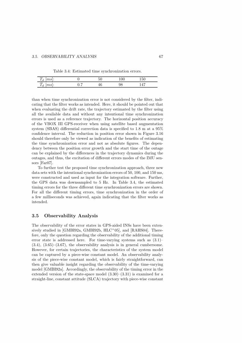
3.5. OBSERVABILITY ANALYSIS 67
Table 3.4: Estimated time synchronization errors.
Td [ms]: 0 50 100 150
Td [ms]: 0.7 46 98 147
than when time synchronization error is not considered by the filter, indi-cating that the filter works as intended. Here, it should be pointed out thatwhen evaluating the drift rate, the trajectory estimated by the filter usingall the available data and without any intentional time synchronizationerrors is used as a reference trajectory. The horizontal position accuracyof the VBOX III GPS-receiver when using satellite based augmentationsystem (SBAS) differential correction data is specified to 1.8 m at a 95%confidence interval. The reduction in position error shown in Figure 3.16should therefore only be viewed as indication of the benefits of estimatingthe time synchronization error and not as absolute figures. The depen-dency between the position error growth and the start time of the outagecan be explained by the differences in the trajectory dynamics during theoutages, and thus, the excitation of different errors modes of the IMU sen-sors [Far07].
To further test the proposed time synchronization approach, three newdata sets with the intentional synchronization errors of 50, 100, and 150 ms,were constructed and used as input for the integration software. Further,the GPS data was downsampled to 5 Hz. In Table 3.4, the estimatedtiming errors for the three different time synchronization errors are shown.For all the different timing errors, time synchronization in the order ofa few milliseconds was achieved, again indicating that the filter works asintended.
3.5 Observability Analysis
The observability of the error states in GPS-aided INSs have been exten-sively studied in [GMBI92a, GMBI92b, HLC+05], and [RAHS04]. There-fore, only the question regarding the observability of the additional timingerror state is addressed here. For time-varying systems such as (3.1)–(3.4), (3.65)–(3.67), the observability analysis is in general cumbersome.However, for certain trajectories, the characteristics of the system modelcan be captured by a piece-wise constant model. An observability analy-sis of the piece-wise constant model, which is fairly straightforward, canthen give valuable insight regarding the observability of the time-varyingmodel [GMBI92a]. Accordingly, the observability of the timing error in theextended version of the state-space model (3.30)–(3.31) is examined for astraight-line, constant attitude (SLCA) trajectory with piece-wise constant

68 CHAPTER 3. TIME SYNCHRONIZATION IN GPS-AIDED INS
acceleration segments, for which the system dynamics can be described bya piece-wise constant model.
The observability analysis of the time synchronization error is carriedout in four steps. First, the definition of observability is stated and amathematical tool to examine the observability is shortly described. Sec-ond, the observability of the GPS-aided INS with the standard error model(3.1)–(3.4), (3.65)–(3.67), is studied during an SLCA trajectory where thenavigation platform experience a constant acceleration. Thereafter, theobservability of the GPS-aided INS with the extended state-space model(3.30)–(3.31) is examined for the same trajectory conditions. Finally, theobservability of the GPS-aided INS with the extended state-space model isexamined for an SLCA trajectory consisting of two constant accelerationsegments. For simplicity, the ratio M between the sampling of the IMUand the GPS-receiver is set to one, throughout the observability analysis.
3.5.1 Observability Definition
A system is said to be observable at time k, if the state vector, xk can bedetermined from the outputs zk, ..., zk+N for a finite N [ÅW84]. By ne-glecting the process noise and measurement noise in the state space model(3.1)–(3.4), this is equivalent to the existence of a unique solution to
qk = W xk (3.43)
whereqk =
[zTk zTk+1 zTk+2 . . . zTk+N
]T(3.44)
and
W =
HkHk+1 Ψk
Hk+2 Ψk+1 Ψk...
Hk+N∏Ni=1 ΨN+k−i
. (3.45)
This will be the case if the observability matrix has full column rank, i.e.,rankW = α. Otherwise, the set Ωxk of possible solutions to (3.43) isgiven by
Ωxk = xk ∈ Rn ; qk = W0 xk
= xk ∈ Rn ; xk = xak + Υ η, η ∈ R
ℓ(3.46)
where W Υ = 0α,ℓ and rank(Υ) = ℓ. Further, xak denotes the true statevector that produced the observations. Here, ℓ is the rank of the nullspace and the columns of Υ span the null space of the observability ma-trix. Hence, if the observability matrix does not have full rank, then the
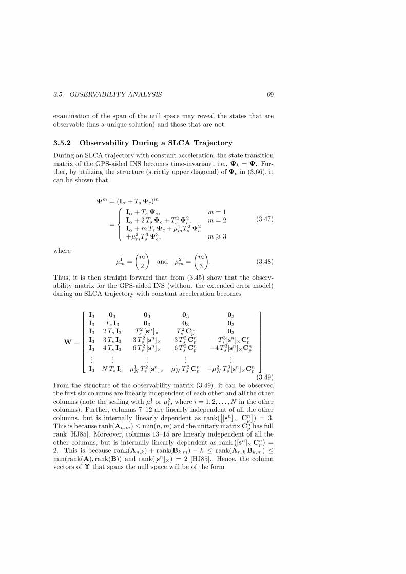
3.5. OBSERVABILITY ANALYSIS 69
examination of the span of the null space may reveal the states that areobservable (has a unique solution) and those that are not.
3.5.2 Observability During a SLCA Trajectory
During an SLCA trajectory with constant acceleration, the state transitionmatrix of the GPS-aided INS becomes time-invariant, i.e., Ψk = Ψ. Fur-ther, by utilizing the structure (strictly upper diagonal) of Ψc in (3.66), itcan be shown that
Ψm = (Iα + TsΨc)m
=
Iα + TsΨc, m = 1Iα + 2TsΨc + T 2
s Ψ2c , m = 2
Iα +mTsΨc + µ1mT
2s Ψ2
c
+µ2mT
3s Ψ3
c , m > 3
(3.47)
where
µ1m =
(m
2
)and µ2
m =
(m
3
). (3.48)
Thus, it is then straight forward that from (3.45) show that the observ-ability matrix for the GPS-aided INS (without the extended error model)during an SLCA trajectory with constant acceleration becomes
W =
I3 03 03 03 03
I3 Ts I3 03 03 03
I3 2Ts I3 T 2s [sn]× T 2
s Cnp 03
I3 3Ts I3 3T 2s [sn]× 3T 2
s Cnp −T 3s [sn]×Cnp
I3 4Ts I3 6T 2s [sn]× 6T 2
s Cnp −4T 3s [sn]×Cnp
......
......
...I3 N Ts I3 µ
1N T
2s [sn]× µ1
N T2s Cnp −µ2
N T3s [sn]×Cnp
(3.49)From the structure of the observability matrix (3.49), it can be observedthe first six columns are linearly independent of each other and all the othercolumns (note the scaling with µ1
i or µ2i , where i = 1, 2, . . . , N in the other
columns). Further, columns 7–12 are linearly independent of all the othercolumns, but is internally linearly dependent as rank(
[[sn]× Cnp
]) = 3.
This is because rank(An,m) ≤ min(n,m) and the unitary matrix Cnp has fullrank [HJ85]. Moreover, columns 13–15 are linearly independent of all theother columns, but is internally linearly dependent as rank
([sn]×Cnp
)=
2. This is because rank(An,k) + rank(Bk,m) − k ≤ rank(An,kBk,m) ≤min(rank(A), rank(B)) and rank([sn]×) = 2 [HJ85]. Hence, the columnvectors of Υ that spans the null space will be of the form

70 CHAPTER 3. TIME SYNCHRONIZATION IN GPS-AIDED INS
Υ1:α,i =
06,1
ζ(1)i
03,1
, i = 1, . . . , 3 (3.50)
and
Υ1:α,i =
[012,1
ζ(2)i
], i = 4, 5 (3.51)
respectively. From the structure of Υ and the description of the set Ωxk ,in (3.46) it can be concluded that for the GPS-aided INS (without theextended error model), during an SLCA trajectory with constant accelera-tion:
• The position and velocity errors are observable.
• The attitude errors and the accelerometer biases can only be deter-mined up to certain linear combinations.
• The gyro biases can only be determined up to certain linear combi-nations.
Given the observability matrix W in (3.49), the observability matrixfor the navigation system with the extended error model Wext, under thesame trajectory conditions, can be determined by noting that
(Ψext)m =
[Ψm 0α,101,α 1
](3.52)
and thereby
Hextm (Ψext)m =[
HmΨm vn0 +mTs an0]. (3.53)
Here, vn0 and an0 denote the initial velocity and acceleration of the nav-igation platform during the trajectory segment, respectively. Hence, theobservability matrix, Wext for the system that also estimates the time syn-chronization error becomes as that given in (3.68) (found in Appendix 3.Cat the end of the chapter). Here, sn0 denotes the specific force correspond-ing to the acceleration an0 of the platform. From (3.68), it is clear that thefirst six columns and the last column now are linearly dependent, since
Wext[
(vn0 )T (an0 )T (09,1)T −1]T
= 03(N+1),1. (3.54)
Therefore, from (3.46), it can be concluded that the time synchronizationerror is only determinable up to a linear combination with certain positionand velocity errors during an SLCA trajectory with constant acceleration.

3.6. CONCLUSIONS 71
Thus, a necessary condition for the time synchronization error to be observ-able is that the vehicle trajectory includes acceleration or heading changes.
Subsequently, let us again consider the case when the movements of thenavigation platform can be approximated by an SLCA trajectory. Further,let us assume that this trajectory can be further divided into two subseg-ments that span from time k to k + N and from time k + N + 1 to theend of the SLCA trajectory, respectively. During the first subsegment, theacceleration of the platform is an0 and during the second subsegment, itis an1 . Hence, the corresponding specific force vectors are sn0 and sn1 , re-spectively. Under these conditions the observability matrix Wext
2 at timek becomes as in (3.69) (found in Appendix 3.C at the end of the chapter).Owing to the change in acceleration, the first six and the last columns areno longer linearly dependent. Moreover, as previously stated, they are alsolinearly independent of all the other columns. Therefore, from (3.46), it canbe concluded that the position, velocity, and time synchronization errorsunder these conditions are observable. Hence, sufficient conditions for thetime synchronization error to be observable are that the vehicle trajectoryshould include acceleration changes.
3.6 Conclusions
The effects of large time synchronization errors in a loosely coupled closed-loop GPS-aided INS with error feedback have been studied in terms of theMSE of the system. These large time synchronization errors may occur inlow-cost systems, where precise time synchronization (e.g., using 1-pulse-per-second from the GPS-receiver) is not possible. Expressions for the MSEof the navigation system, given the vehicle trajectory and a state-spacemodel of the error plant of the integrated navigation system, have beenderived. In addition, under the assumption of Gaussian-distributed esti-mates, an MSE expression when the time synchronization error is includedin the feedback loop of the navigation filter has also been determined.
The use of the two MSE expressions is illustrated by applying them toan example of a one-dimensional, GPS-aided INS with an inherent timesynchronization error. The results from the example show that by ex-tending the error model used in the navigation filter to include a state forthe timing error as well, the effects of the timing error become negligi-ble as the filter converges. The accuracy of the derived MSE expressionsis illustrated by MC simulations of the one-dimensional GPS-aided INS,which shows good agreement with the analytical results calculated fromthe derived MSE models. Moreover, a practical approach on how to im-plement the variable delay for time synchronization of the IMU and theGPS-receiver data is also briefly discussed.
Furthermore, the proposed time synchronization approach using a frac-
72 CHAPTER 3. TIME SYNCHRONIZATION IN GPS-AIDED INS
tional delay filter to interpolate the IMU data was implemented as a partof the software developed in-house for the integration of the GPS and IMUdata. The time synchronization was then tested on both simulated and real-world data. When the timing error was not considered by the integrationsoftware, the MSE calculated by MC simulations was in agreement withthat predicted by the derived MSE expression. However, when the timingerror was considered by the integration filter, the derived MSE expressionsfailed to fully capture the transient behavior of the filter. However, as thefilter converged, the agreement improved and the effects of the timing errorwere removed. In the test with real-world data, with intentionally includedtiming errors, time synchronization within a few milliseconds was obtained.Further, the differences in arithmetic mean error during the simulated GPSoutages indicated that the sensor biases were better estimated when thetiming error was considered by the integration filter (i.e., no bias in theestimated forward acceleration).
To conclude, large synchronization errors in the sampling instances ofthe GPS-receiver and the IMU sensor in a GPS-aided INS are observed toseriously degrade the performance of the system. The derived MSE ex-pression provides an efficient way of evaluating the systems performancefor a certain timing error and vehicle trajectory. By extending the inte-gration filter to estimate the timing error also, and by feeding back theestimates to synchronize the GPS-receiver and the IMU data by means ofa fractional delay filter, almost perfect time synchronization (in the orderof a few milliseconds) can be achieved and the effects of the timing errorcan be cancelled. Hence, the proposed synchronization method can pro-vide a substantial improvement to the accuracy of the navigation solutionfor loosely coupled GPS-aided INS with large timing errors, whereas, forthe system already synchronized within a few milliseconds, the proposedmethod brings marginal, if any, improvement to the accuracy of the navi-gation solution.

3.A. EXTENDED STATE SPACE MODEL ERROR COVARIANCE 73
3.A Extended State Space Model Error Covariance
From the derived difference equation (3.38) for the error in the system withthe extended state-space model, the MSE of the system can be written as
Pextfd,k+1 = Exe,extfd,k+1 (xe,extfd,k+1)T = Φextk Pextfd,k (Φextk )T + Kextp,k R (Kextk )T
+ Gextk Q (Gextk )T + Kextp,k Πk (Kextk )T
−Φextk Γk (Kextk )T −Kextp,k ΓTk (Φextk )T
(3.55)
where
Πk = Edextk (dextk )T =ak aTk
4EδT 4
d,k (3.56)
and
Γk = Exextfd,k (dextk )T = Exextfd,k δT 2d,k
aTk2. (3.57)
By assuming the state estimates to be Gaussian-distributed, (3.56) and(3.57) can be rewritten in terms of Pextfd,k and xextfd,k = Exextfd,k by usingthe equalities found in [BD71]. That is, EδT 4
d,k in (3.56) can be expressedas
EδT 4d,k = 3 EδT 2
d,k2 − 2 EδTd,k4. (3.58)
By inserting (3.58) into (3.56), Πk can be written as
Πk =ak aTk
4EδT 4
d,k
=ak aTk
4
(3 EδT 2
d,k2 − 2 EδTd,k4)
=ak aTk
4
(3 [Pextfd,k]
2i,i − 2 [xextfd,k]
4i
).
(3.59)
Further, EδT 2d,k xextf,k in (3.57) can be rewritten as
EδT 2d,k [xextfd,k]j = EδT 2
d,kE[xextfd,k]j
+ 2 EδTd,k(E[xextfd,k]j δTd,k
− EδTd,kE[xextfd,k]j).
(3.60)

74 CHAPTER 3. TIME SYNCHRONIZATION IN GPS-AIDED INS
Equation (3.60) can be expressed in terms of the MSE matrix Pextfd,k andmean value vector xextfd,k as
EδT 2d,k [xextfd,k]j = [Pextfd,k]i,i [x
extfd,k]j + 2 [xextfd,k]i
· ([Pextfd,k]j,i − [xextfd,k]i [xextfd,k]j).
(3.61)
Thus, the expected value of the vector EδT 2d,k xextfd,k is given by
EδT 2d,k xextfd,k = [Pextfd,k]i,i xextfd,k + [xextfd,k]i
· ( [Pextfd,k]1:α,i − [xextfd,k]i xextfd,k ).
(3.62)
As given earlier, α is the length of the state vector. Inserting this into (3.57),then Γk can be written as
Γk =(
[Pextfd,k]i,i xextfd,k + 2 [xextfd,k]i
· ( [Pextfd,k]1:α,i − [xextfd,k]i xextfd,k )) aTk
2
(3.63)
where
xextfd,k = Φextk xextfd,k −Kextp,k Edextk
= Φextk xextfd,k −1
2Kextp,k ak [Pextfd,k]i,i
(3.64)
and Φextk = (Ψextk −Kextp,k Hextk ). Thus, under the assumption of Gaussian-distributed state estimates, the MSE of the estimated state vector in thenavigation system with the augmented state vector, recursively, can becalculated from (3.55), (3.59), (3.63), and (3.64).
3.B INS Error Model
The following is the error model used in the software for integrating GPSand IMU data. Let the error state vector be defined as
xc =[
(δpn)T (δvn)T θT (δf b)T (δωpip)T]T. (3.65)
Here, δpn and δvn denotes the position and velocity error, respectively.The superscript n indicates that the variables are described in the naviga-tion coordinate frame. Further, the vector θ contains the roll, pitch, andheading error. The accelerometer and gyroscope sensor errors in platformcoordinates are denoted as δfp and δωpip, respectively. With the above-described state vector, the continuous-time state transition matrix of thesystem becomes
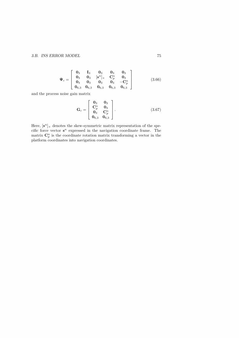
3.B. INS ERROR MODEL 75
Ψc =
03 I3 03 03 03
03 03 [sn]× Cnp 03
03 03 03 03 −Cnp06,3 06,3 06,3 06,3 06,3
(3.66)
and the process noise gain matrix
Gc =
03 03
Cnp 03
03 Cnp06,3 06,3
. (3.67)
Here, [sn]× denotes the skew-symmetric matrix representation of the spe-cific force vector sn expressed in the navigation coordinate frame. Thematrix Cnp is the coordinate rotation matrix transforming a vector in theplatform coordinates into navigation coordinates.

76C
HA
PT
ER
3.T
IME
SY
NC
HR
ON
IZA
TIO
NIN
GP
S-A
IDE
DIN
S
3.C
Ob
servab
ilityM
atr
ices
Wext =
I3 03 03 03 03 vn0I3 Ts I3 03 03 03 vn0 + Ts an0I3 2Ts I3 T 2
s [sn0 ]× T 2s Cnp 03 vn0 + 2Ts an0
I3 3Ts I3 3T 2s [sn0 ]× 3T 2
s Cnp −T 3s [sn0 ]×Cnp vn0 + 3Ts an0
I3 4Ts I3 6T 2s [sn0 ]× 6T 2
s Cnp −4T 3s [sn0 ]×Cnp vn0 + 4Ts an0
......
......
......
I3 N Ts I3 µ1N T
2s [sn0 ]× µ1
N T2s Cnp −µ2
N T3s [sn0 ]×Cnp vn0 +N Ts an0
(3.68)
Wext2 =
I3 03 03 03 03 vn0I3 Ts I3 03 03 03 vn0 + Ts an0I3 2Ts I3 T 2
s [sn0 ]× T 2s Cnp 03 vn0 + 2Ts an0
I3 3Ts I3 3T 2s [sn0 ]× 3T 2
s Cnp T 3s [sn0 ]×Cnp vn0 + 3Ts an0
I3 4Ts I3 6T 2s [sn0 ]× 6T 2
s Cnp −4T 3s [sn0 ]×Cnp v0 + 4Ts an0
......
......
......
I3 N Ts I3 µ1N T
2s [sn0 ]× µ1
N T2s Cnp −µ2
N T3s [sn0 ]×Cnp vn0 +N Ts an0
I3 (N + 1)Ts I3 T2s (µ1N [sn0 ]× +N [sn1 ]×) µ1
N+1T2sCnp −µ2
N+1 T3s [sn0 ]×Cnp vn0 + Ts (N an0 + an1 )
......
......
......
(3.69)

Chapter 4
Synchronization by Message
Exchanges
4.1 Introduction
Within wireless sensor networks (WSNs), a common notation of time be-tween network nodes is essential for many applications. Therefore, a largeamount of research has been carried out in the field of time synchroniza-tion within WSNs. The result is a diverse set of time synchronizationalgorithms and protocols such as: Timing-synch Protocol for Sensor Net-works (TPSN) [GKS03], TSync [DH04], Flooding Time SynchronizationProtocol (FTSP) [MKSL04], and Time Synchronization for High Latency(TSHL) [SH06b]. For a detailed description of different time synchroniza-tion protocols within WSNs, refer to [SBK05, SSBNS08, SY04]. A varietyof error sources set a bound on the achievable performance of a performedclock synchronization. Bounds for the achievable clock synchronization ac-curacy using different protocols and clock models have been derived undera variety of assumptions [YZC05, NCSS07, LL84, CSQ08a, NSQ08, Tru01].
The study presented in this chapter considers clock synchronizationwith the aid of a two-way message exchange between a master unit and aplurality of slave units, as illustrated in Fig. 4.1. The setup in Fig. 4.1 iscommon in a variety of applications, for example offshore submarine posi-tioning, as studied in some detail at the end of the chapter. The slave nodesare assumed to have no common time reference, i.e., they all have their lo-cal oscillator providing them with the local time. Thus, it is sufficient tostudy the two-way synchronization message exchange between the masterand an arbitrary slave unit. In the study, the theoretical achievable clocksynchronization accuracy between a master and slave node is examined,subject to a two-way clock message exchange, where the synchronizationrequests are periodically repeated. Further, a low complexity estimator is
77
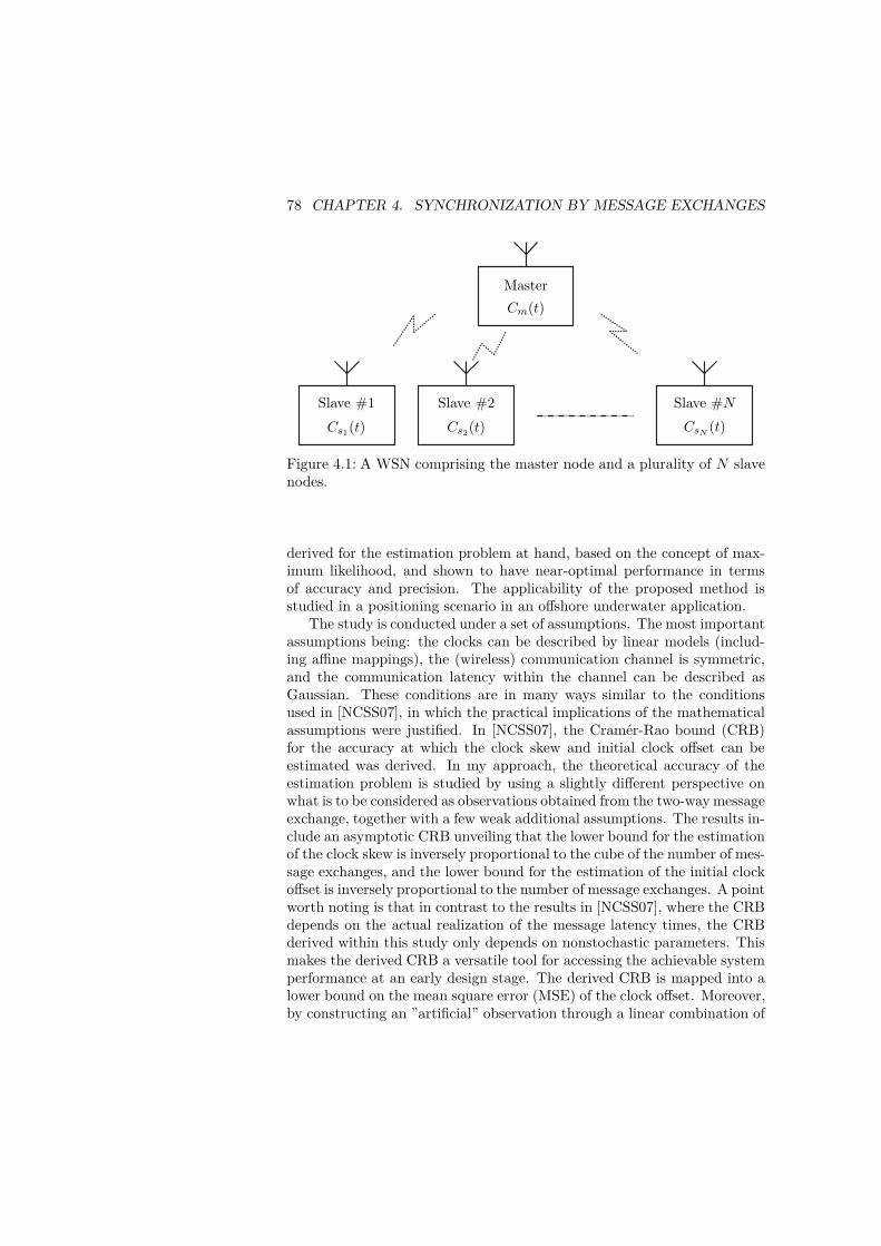
78 CHAPTER 4. SYNCHRONIZATION BY MESSAGE EXCHANGES
Master
Slave #1 Slave #2 Slave #N
Cm(t)
Cs1(t) Cs2(t) CsN (t)
Figure 4.1: A WSN comprising the master node and a plurality of N slavenodes.
derived for the estimation problem at hand, based on the concept of max-imum likelihood, and shown to have near-optimal performance in termsof accuracy and precision. The applicability of the proposed method isstudied in a positioning scenario in an offshore underwater application.
The study is conducted under a set of assumptions. The most importantassumptions being: the clocks can be described by linear models (includ-ing affine mappings), the (wireless) communication channel is symmetric,and the communication latency within the channel can be described asGaussian. These conditions are in many ways similar to the conditionsused in [NCSS07], in which the practical implications of the mathematicalassumptions were justified. In [NCSS07], the Cramér-Rao bound (CRB)for the accuracy at which the clock skew and initial clock offset can beestimated was derived. In my approach, the theoretical accuracy of theestimation problem is studied by using a slightly different perspective onwhat is to be considered as observations obtained from the two-way messageexchange, together with a few weak additional assumptions. The results in-clude an asymptotic CRB unveiling that the lower bound for the estimationof the clock skew is inversely proportional to the cube of the number of mes-sage exchanges, and the lower bound for the estimation of the initial clockoffset is inversely proportional to the number of message exchanges. A pointworth noting is that in contrast to the results in [NCSS07], where the CRBdepends on the actual realization of the message latency times, the CRBderived within this study only depends on nonstochastic parameters. Thismakes the derived CRB a versatile tool for accessing the achievable systemperformance at an early design stage. The derived CRB is mapped into alower bound on the mean square error (MSE) of the clock offset. Moreover,by constructing an ”artificial” observation through a linear combination of

4.2. PROBLEM DESCRIPTION 79
the original observations, a low-complexity, approximate maximum likeli-hood estimator (AMLE) is derived and its performance investigated.
4.2 Problem Description
Let the functions Cm(τ) and Cs(τ) describe the clock states as a functionof the time τ for the master and slave node, respectively. The clock offsetat time τ between the two clocks is then defined as
∆(τ) = Cs(τ)− Cm(τ). (4.1)
The aim of the following analysis is to provide a lower bound for the errorvariance at which the clock offset can be estimated using a two-way mes-sage exchange between the nodes and methods for estimation. The boundis applicable under the following two assumptions regarding the clocks ofthe nodes:
A.1 The clock resolution of the nodes is considered infinite, i.e., the clocksCm(τ) and Cs(τ) are modelled by continuous time functions.
A.2 The clocks are assumed to have constant skews and initial offsets, butno other errors.
In practice, the clocks revolve with discrete time steps proportional tothe inverse of the frequency of the oscillator driving the clock register.However, assumption A.1 is valid if the step size of the clock is small incomparison with the time duration of the events that the clock is measuring.Refer to [Sad06] for details on the practical effect that the limited clockresolution imposes on the clock synchronization problem. The validity ofA.2 can be related to a local time interval for which the assumptions holdtrue, i.e., the model errors should be small when compared with the timeframe spanned by the employed clock skew estimation algorithm.
Next, let the time indicated by the master clock Cm(τ) be the localreference time1 t of the system, i.e., t ≡ Cm(τ). Then, given assumptionsA.1 and A.2 the clock state of the slave node as a function of the referencetime t may be modeled as
Cs(t) = (1 + α) t+ β. (4.2)
Here, α denotes the clock skew relative to the master node clock. Further,β is the offset between the slave node clock and the master node clock at
1Note that the duration of a ”second” in the local reference time differs from theSI-unit definition of a second. However, for simplicity, the author allow a slight misuseof units when specifying the duration of time events.

80 CHAPTER 4. SYNCHRONIZATION BY MESSAGE EXCHANGES
0 500 1000 1500 2000 2500 3000 3500−0.25
−0.2
−0.15
−0.1
−0.05
0
0 500 1000 1500 2000 2500 3000 3500−1
−0.5
0
0.5
1
1.5x 10
−5
Clock offset as a function of time.
Clock offsetLinear fit
Residual from linear fit.
Res
idua
l[s
]C
lock
offse
t[s
]
Time [s]
Time [s]
Figure 4.2: Clock offset between the clock of an AVR ATmega 8 µ-controllerwith a 3.6854 Mhz quartz crystal controlled clock oscillator, and the clockof a GlobalSat EM-411 GPS-receiver module, and the residual of a linearfit to the clock offset. The clock skew is in the order of −60 [µs/s].
t = 0. In the sequel, β is referred to as the initial clock offset. Clock modelssimilar to (4.2) are used in, e.g., [SY04, NCSS07, Sad06]. The offset (as afunction of the local reference time t between the master and slave nodeclocks can be described as
∆(t) = Cs(t)− Cm(t) = α t+ β. (4.3)
With reference to (4.3), determining the clock offset is under assumptionsA.1 and A.2 equivalent to estimating the clock skew α and the initial clockoffset β of the slave node clock. In Figure 4.2, the clock offset between aclock of a micro controller and the clock of a GPS-receiver during one houris shown together with the residual of a least-squares fit of the model in (4.3)to the clock offset. Even though the correlation in the residual indicatesthat the model does not resemble the full picture of the clock’s behavior,the model describes the main characteristics and justifies the use of theemployed model for the forthcoming analysis. For a description of morerefined clock models and their characteristics, refer to [All87, All84, Bre97].

4.3. THE TWO-WAY MESSAGE EXCHANGE MODEL 81
Cs(t)
t ≡ Cm(τ)
Cs(t(2)n ) Cs(t
(3)n )
t(1)n t
(2)n t
(3)n t
(4)n
T(1)n T
(2)n
ǫn
Reque
st Reply
Figure 4.3: Illustration of the two-way message exchange model.
4.3 The Two-Way Message Exchange Model
In the two-way message exchange model for time synchronization, as illus-trated in Figure 4.3, the master node starts at time t(1)
n by sending thenth message with a request concerning the current clock state of the slavenode. After a transmission delay T (1)
n , the slave receives the request at timet(2)n and reads its own clock state Cs(t
(2)n ). After ǫn seconds, i.e., at time
t(3)n , the slave node replies by returning the two clock states Cs(t
(2)n ) and
Cs(t(3)n ) to the master node. After a delay T (2)
n , the master node receivesthe reply and reads its own clock state t(4)
n .
4.3.1 Prerequisites
Let the following assumptions regarding the communication between thenodes hold true:
A.3 The clock state can be communicated from the slave node to the mas-ter node with infinite resolution.
Then, the observations available at the master node after each messageexchange starting at t(1)
n are given by
z(1)n = Cs(t
(2)n ), (4.4)
z(2)n = Cs(t
(3)n ), (4.5)
82 CHAPTER 4. SYNCHRONIZATION BY MESSAGE EXCHANGES
and
z(3)n = t(4)
n . (4.6)
Having received the observations, the master node is to estimate the skewα and initial offset β. The accuracy at which this may be done dependson the probability distribution function (PDF) of the observations and theprior knowledge about the shape parameters of the distribution.
In the two-way message exchange model, there are three nondetermin-istic quantities, with corresponding PDFs, which determine the probabilitydistribution of the observations. First, there are the two end-to-end mes-sage latencies T (1)
n and T (2)n , which in addition to the actual propagation
delay across the communication channel, also account for the time neededto prepare and process the message, access the channel, and interpret themessage together with reading the clock state at the receiving node. Referto [GKS03, MAP07, YZC05, EGE02] for a discussion on the causes andcharacteristics of the latency sources mentioned above. Then, there is alsothe slave node reply delay ǫn, which depends on the scheduling and currentprocess load of the slave node. Note that the introduction of ǫn, into themodel of the two-way message exchange (when compared with the modelused in [NCSS07]) is the key step in deriving a CRB only dependent onpredefined system parameters. Next, introduce the following four assump-tions regarding the PDFs of the quantities discussed earlier:
A.4 The communication channel between the master and slave node is sym-metric, and the message delays T (1)
n and T (2)n are ruled by the same
distribution.
A.5 The combined uncertainty of the nondeterministic quantities includedin each message delay may be modeled as Gaussian-distributed, i.e.,T
(i)n ∼ N (µT , σT ) for i = 1, 2, where the mean µT and standard devi-
ation σT fulfill the condition µT ≫ σT .
A.6 The delay ǫn is Gaussian-distributed with mean µǫ and standard de-viation σǫ, where µǫ ≫ σǫ.
A.7 The delays T (1)n , T (2)
n and ǫn are mutually independent stochastic vari-ables and i.i.d. with respect to n.
The condition on the mean to be much larger than the standard deviationin assumptions A.5 and A.6 is because the probability for T (1)
n , T (2)n , and

4.3. THE TWO-WAY MESSAGE EXCHANGE MODEL 83
ǫn to be negative should be sufficiently close to zero. The assumption mayseem to be imprecise, due to a nonzero probability for negative delays. Forthe practical scenarios considered, the assumption is a natural trade-off be-tween reasonability and our efforts to tackle the mathematical issues. Theassumption regarding Gaussian distribution is partly arguable and othercommon distributions used to model the message latencies are the Gammadistribution (having the chi-squared, exponential, and Erlang distribu-tion as special cases [EHP00]), and the log-normal distribution [CSQ08b].In [YZC05], both uniformly and exponentially distributed message delaysare considered in the analysis of the clock synchronization accuracy withina WSN. However, the Gaussian assumption may be motivated by the cen-tral limit theorem, if the delays are viewed to be the addition of numerousindependent delays originating from the channel, scheduling, processing,etc. [LKS08, NSQ08]. Gaussian-distributed message delays are motivatedand employed, for example in [vGR03, XK09, GBH04, CLYX06]. One maynote in [GvCCS05] that the end-to-end message delays in the communica-tion between Micro2 Motes were measured. The statistics of the observeddata fitted, at a 99.97% confidence interval, a Gaussian distribution with amean of 762 µs and standard deviation of 2.82 µs. Accordingly, the Gaus-sian distribution is indeed relevant in several applications, and the aboveassumptions are justified.
4.3.2 Time Stamp Observations
Next, a model for the observations is derived. Rewriting the observations(4.4), (4.5), and (4.6) in terms of t(1)
n , T (1)n , T (2)
n , and ǫn yield
z(1)n = Cs(t
(1)n + T (1)
n ) (4.7)
z(2)n = Cs(t
(1)n + ǫn + T (1)
n ) (4.8)
and
z(3)n = t(1)
n + ǫn + T (1)n + T (2)
n . (4.9)
The clock model in (4.2) implies that the observations are linear combina-tions of Gaussian-distributed random variables. Let
zn =[z
(1)n z
(2)n z
(3)n
]T, (4.10)
where (·)T denotes the transpose operation. Then, the vector of observa-tions zn ∼ N (un(θ),R(θ)), with the mean given by
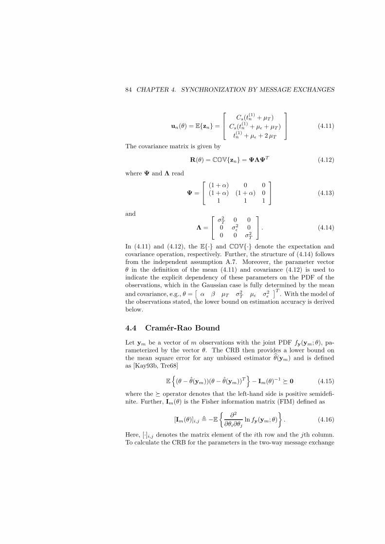
84 CHAPTER 4. SYNCHRONIZATION BY MESSAGE EXCHANGES
un(θ) = Ezn =
Cs(t
(1)n + µT )
Cs(t(1)n + µǫ + µT )
t(1)n + µǫ + 2µT
(4.11)
The covariance matrix is given by
R(θ) = COVzn = ΨΛΨT (4.12)
where Ψ and Λ read
Ψ =
(1 + α) 0 0(1 + α) (1 + α) 0
1 1 1
(4.13)
and
Λ =
σ2T 0 00 σ2
ǫ 00 0 σ2
T
. (4.14)
In (4.11) and (4.12), the E· and COV· denote the expectation andcovariance operation, respectively. Further, the structure of (4.14) followsfrom the independent assumption A.7. Moreover, the parameter vectorθ in the definition of the mean (4.11) and covariance (4.12) is used toindicate the explicit dependency of these parameters on the PDF of theobservations, which in the Gaussian case is fully determined by the meanand covariance, e.g., θ =
[α β µT σ2
T µǫ σ2ǫ
]T. With the model of
the observations stated, the lower bound on estimation accuracy is derivedbelow.
4.4 Cramér-Rao Bound
Let ym be a vector of m observations with the joint PDF fy(ym; θ), pa-rameterized by the vector θ. The CRB then provides a lower bound onthe mean square error for any unbiased estimator θ(ym) and is definedas [Kay93b, Tre68]
E
(θ − θ(ym))(θ − θ(ym))T
− Im(θ)−1 0 (4.15)
where the operator denotes that the left-hand side is positive semidefi-nite. Further, Im(θ) is the Fisher information matrix (FIM) defined as
[Im(θ)]i,j , −E
∂2
∂θi∂θjln fy(ym; θ)
. (4.16)
Here, [·]i,j denotes the matrix element of the ith row and the jth column.To calculate the CRB for the parameters in the two-way message exchange

4.4. CRAMÉR-RAO BOUND 85
model, let the vector ym ∈ R3m contain the observations obtained from mexecutions of the message exchange procedure. That is
ym =[
zT0 . . . zTm−1
]T(4.17)
where the single-message observation zn was given in (4.10). Next, as-sumption A.7 implies that the observations obtained from the differentexecutions are independent. Thus, it holds that
fy(ym; θ) =
m−1∏
n=0
fzn(zn; θ), (4.18)
where fzn(zn; θ) is the Gaussian PDF of the observations at the nth exe-cutions of the message exchange procedure. Inserting (4.18) into the ex-pression for the FIM in (4.16) yields
[Im(θ)]i,j =m−1∑
n=0
[Jn(θ)]i,j , (4.19)
where
[Jn(θ)]i,j = −E
∂2
∂θi∂θjln fzn(zn; θ)
. (4.20)
Further, since the observations are obeying a Gaussian distribution it holdsthat [Kay93b]
[Jn(θ)]i,j =
[∂un(θ)
∂θi
]TR−1(θ)
[∂un(θ)
∂θj
]
+1
2tr(
R−1(θ)∂R(θ)
∂θiR−1(θ)
∂R(θ)
∂θj
). (4.21)
where un(θ) and R(θ) are explicitly given in (4.11) and (4.12), respectively.Further, tr(·) denotes the trace operation. Inserting (4.21) into (4.19),evaluating the finite sum yields an expression for the FIM. The lower boundon accuracy then follows by a matrix inversion.
4.4.1 CRB for Four Different Scenarios
The objective of the two-way message exchange for clock synchronizationis to estimate the clock skew α and the initial clock offset β. However,depending on the prior knowledge about the means and variances of thedelays in the message exchange, nuisance parameters must be estimated aswell. The following four cases will be examined in some detail:

86 CHAPTER 4. SYNCHRONIZATION BY MESSAGE EXCHANGES
C.1 Known channel and processing delay. The first- and second-order mo-ment of the delays T (1)
n , T (2)n , and ǫn are known, i.e., θ =
[α β
]T.
C.2 Known processing delay. The mean and variance of ǫn are known butmean and variance of the message delays T (1)
n and T (2)n are unknown,
i.e., θ =[α β µT σ2
T
]T.
C.3 Known channel delay. The mean and variance of T (1)n and T (2)
n areknown, but mean and variance of the processing delays ǫn are un-known, i.e., θ =
[α β µǫ σ
2ǫ
]T.
C.4 No prior knowledge. The means and variances of all delays are un-known, i.e., θ =
[α β µT σ2
T µǫ σ2ǫ
]T.
Straightforward but tedious calculations reported in [SH09b], evaluating(4.21) for case C.1 yields
[Jn(θ)]1,1 =2 (t
(1)n + µT )2
(1 + α)2σ2T
+2 (t
(1)n + µT )µǫ
(1 + α)2σ2T
+µ2ǫ + σ2
ǫ
(1 + α)2σ2T
+5σ2ǫ + µ2
ǫ
(1 + α)2σ2ǫ
,
(4.22)
[Jn(θ)]1,2 = [Jn(θ)]2,1 =2 (t
(1)n + µT ) + µǫ(1 + α)2 σ2
T
, (4.23)
and
[Jn(θ)]2,2 =2
(1 + α)2 σ2T
. (4.24)
Here, (4.22) and (4.23) depend on the known starting time t(1)n of the nth
message exchange. To proceed, introduce the following assumption regard-ing the starting time of each message exchange:
A.8 The master node sends a request to the slave node regarding the cur-rent clock state with a periodicity of Ts seconds, i.e., t(1)
n = nTs forn = 0, . . . ,m− 1.

4.4. CRAMÉR-RAO BOUND 87
Note that for the two-way message exchange model to be valid, Ts must bechosen so large that the statistics of delays are unaffected by the communi-cation and processor load induced by the synchronization message exchangeitself. Otherwise, a more sophisticated model for the message exchange isrequired. With assumption A.8, the four elements of the FIM for case C.1become
[Im(θ)]1,1 =T 2s m (2m− 1)(m− 1)
3 (1 + α)2σ2T
+Tsm (m− 1)(2µT + µǫ)
(1 + α)2σ2T
+m(2µ2T + 2µTµǫ + µ2
ǫ + 5σ2T + σ2
ǫ
)
(1 + α)2σ2T
+mµ2
ǫ
(1 + α)2σ2ǫ
,
(4.25)
[Im(θ)]1,2 = [Im(θ)]2,1 =m(µǫ + 2µT + Ts (m− 1))
(1 + α)2 σ2T
, (4.26)
and
[Im(θ)]2,2 =2m
(1 + α)2 σ2T
. (4.27)
For cases C.2–C.4, the additional nonzero elements of the correspondingFIMs are reported in Appendix 4.A. The final step in calculating theCRBs for the different cases are the inversion of the four different FIMs.The inversions may be done analytically, for example using computationalsoftware such as Mathematica. The resulting expressions are extensive, andtherefore, only the parts related to the bound on the variance of the clockskew α and the initial clock offset β are presented. The matrix inverses asa whole are reported in [SH09b]. Let i (for i = 1, . . . , 4) denote the caseunder consideration, then
[I−1m (θ)
]1,1
=6 (1 + α)2 σ2
T σ2ǫ
σ2ǫ (m
2 − 1)mT 2s + ci(m)
, (4.28)
[I−1m (θ)
]1,2
=[I−1m (θ)
]2,1
= −3 (1 + α)2 σ2T σ
2ǫ ((m− 1)Ts + 2µT + µǫ)
σ2ǫ (m
2 − 1)mT 2s + ci(m)
,(4.29)
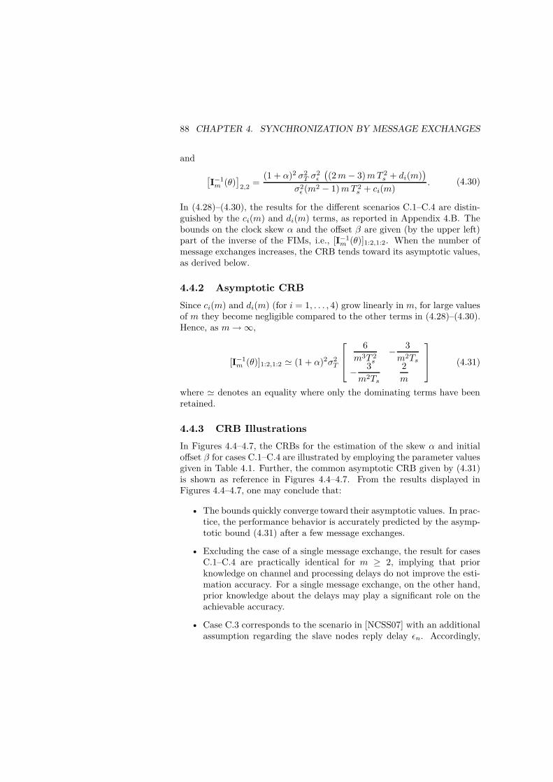
88 CHAPTER 4. SYNCHRONIZATION BY MESSAGE EXCHANGES
and
[I−1m (θ)
]2,2
=(1 + α)2 σ2
T σ2ǫ
((2m− 3)mT 2
s + di(m))
σ2ǫ (m
2 − 1)mT 2s + ci(m)
. (4.30)
In (4.28)–(4.30), the results for the different scenarios C.1–C.4 are distin-guished by the ci(m) and di(m) terms, as reported in Appendix 4.B. Thebounds on the clock skew α and the offset β are given (by the upper left)part of the inverse of the FIMs, i.e., [I−1
m (θ)]1:2,1:2. When the number ofmessage exchanges increases, the CRB tends toward its asymptotic values,as derived below.
4.4.2 Asymptotic CRB
Since ci(m) and di(m) (for i = 1, . . . , 4) grow linearly in m, for large valuesof m they become negligible compared to the other terms in (4.28)–(4.30).Hence, as m→∞,
[I−1m (θ)]1:2,1:2 ≃ (1 + α)2σ2
T
6
m3T 2s
− 3
m2Ts
− 3
m2Ts
2
m
(4.31)
where ≃ denotes an equality where only the dominating terms have beenretained.
4.4.3 CRB Illustrations
In Figures 4.4–4.7, the CRBs for the estimation of the skew α and initialoffset β for cases C.1–C.4 are illustrated by employing the parameter valuesgiven in Table 4.1. Further, the common asymptotic CRB given by (4.31)is shown as reference in Figures 4.4–4.7. From the results displayed inFigures 4.4–4.7, one may conclude that:
• The bounds quickly converge toward their asymptotic values. In prac-tice, the performance behavior is accurately predicted by the asymp-totic bound (4.31) after a few message exchanges.
• Excluding the case of a single message exchange, the result for casesC.1–C.4 are practically identical for m ≥ 2, implying that priorknowledge on channel and processing delays do not improve the esti-mation accuracy. For a single message exchange, on the other hand,prior knowledge about the delays may play a significant role on theachievable accuracy.
• Case C.3 corresponds to the scenario in [NCSS07] with an additionalassumption regarding the slave nodes reply delay ǫn. Accordingly,

4.4. CRAMÉR-RAO BOUND 89
100
101
102
100
105
100
101
102
100
105
CRB case C.1
CRB case C.2Asymptotical CRB
Asymptotical CRB
√M
SE[µs/s]
√M
SE[µs/s]
CRB for α given parameterizations case C.1.
CRB for α given parameterizations case C.2.
Number of message exchanges m
Number of message exchanges m
Figure 4.4: CRBs for α given parametrization case C.1 and C.2 togetherwith the asymptotical CRB for α.
it is relevant to compare the arithmetic mean of the CRB derivedin [NCSS07], with the closed-form results derived herein. The com-parison is given in Figure 4.8, from which one may note an excellentagreement.
The bounds on the parameters α and β are often not as interesting asthe bound on the actual clock offset and how well it may be predicted,which can be found by a proper variable transformation.
4.4.4 A Lower Bound on the Clock Offset
The CRB for the clock parameters can be used to derive a lower bound onMSE for the clock offset estimation. Let θ(ym) be an unbiased estimator ofthe unknown parameters, i.e., clock skew, initial clock offset, etc., based onthe observations obtained fromm message exchanges. Note that parameterestimate m will be available at some time instant t such that t ≥ tm, wheretm = (m− 1)Ts + ηm = t
(1)m−1 + ηm and ηm denote the sum of the round-
trip delays for the mth message exchange, including the processing timeneeded to calculate the estimate. Thus, the mth update of the clock offset
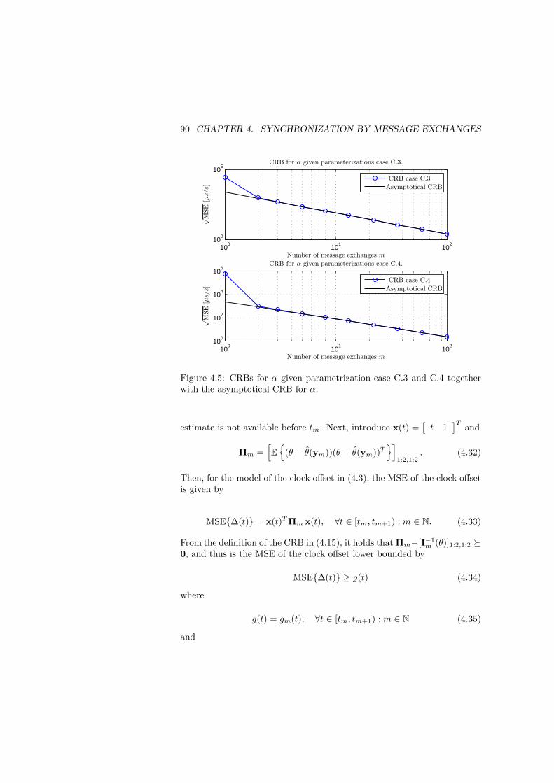
90 CHAPTER 4. SYNCHRONIZATION BY MESSAGE EXCHANGES
100
101
102
100
105
100
101
102
100
102
104
106
CRB case C.3
CRB case C.4Asymptotical CRB
Asymptotical CRB
√M
SE[µs/s]
√M
SE[µs/s]
CRB for α given parameterizations case C.3.
CRB for α given parameterizations case C.4.
Number of message exchanges m
Number of message exchanges m
Figure 4.5: CRBs for α given parametrization case C.3 and C.4 togetherwith the asymptotical CRB for α.
estimate is not available before tm. Next, introduce x(t) =[t 1
]Tand
Πm =[E
(θ − θ(ym))(θ − θ(ym))T
]
1:2,1:2. (4.32)
Then, for the model of the clock offset in (4.3), the MSE of the clock offsetis given by
MSE∆(t) = x(t)TΠm x(t), ∀t ∈ [tm, tm+1) : m ∈ N. (4.33)
From the definition of the CRB in (4.15), it holds that Πm−[I−1m (θ)]1:2,1:2
0, and thus is the MSE of the clock offset lower bounded by
MSE∆(t) ≥ g(t) (4.34)
where
g(t) = gm(t), ∀t ∈ [tm, tm+1) : m ∈ N (4.35)
and
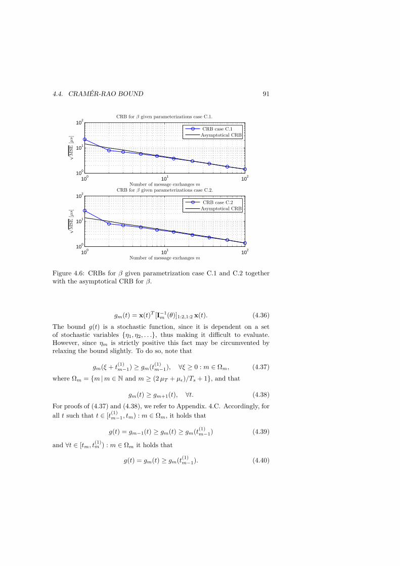
4.4. CRAMÉR-RAO BOUND 91
100
101
102
100
101
102
100
101
102
100
101
102
CRB case C.1
CRB case C.2Asymptotical CRB
Asymptotical CRB
√M
SE[µs]
√M
SE[µs]
CRB for β given parameterizations case C.1.
CRB for β given parameterizations case C.2.
Number of message exchanges m
Number of message exchanges m
Figure 4.6: CRBs for β given parametrization case C.1 and C.2 togetherwith the asymptotical CRB for β.
gm(t) = x(t)T [I−1m (θ)]1:2,1:2 x(t). (4.36)
The bound g(t) is a stochastic function, since it is dependent on a setof stochastic variables η1, η2, . . ., thus making it difficult to evaluate.However, since ηm is strictly positive this fact may be circumvented byrelaxing the bound slightly. To do so, note that
gm(ξ + t(1)m−1) ≥ gm(t
(1)m−1), ∀ξ ≥ 0 : m ∈ Ωm, (4.37)
where Ωm = m |m ∈ N and m ≥ (2µT + µǫ)/Ts + 1, and that
gm(t) ≥ gm+1(t), ∀t. (4.38)
For proofs of (4.37) and (4.38), we refer to Appendix. 4.C. Accordingly, forall t such that t ∈ [t
(1)m−1, tm) : m ∈ Ωm, it holds that
g(t) = gm−1(t) ≥ gm(t) ≥ gm(t(1)m−1) (4.39)
and ∀t ∈ [tm, t(1)m ) : m ∈ Ωm it holds that
g(t) = gm(t) ≥ gm(t(1)m−1). (4.40)

92 CHAPTER 4. SYNCHRONIZATION BY MESSAGE EXCHANGES
100
101
102
100
101
102
100
101
102
100
101
102
103
CRB case C.3
CRB case C.4Asymptotical CRB
Asymptotical CRB
√M
SE[µs]
√M
SE[µs]
CRB for β given parameterizations case C.3.
CRB for β given parameterizations case C.4.
Number of message exchanges m
Number of message exchanges m
Figure 4.7: CRBs for β given parametrization case C.3 and C.4 togetherwith the asymptotical CRB for β.
Table 4.1: Parameter values used in simulations and numerical examples.
Parameter Value Unitα 50 [µs/s]µT 1 [ms]σT 10 [µs]µǫ 0.5 [ms]σǫ 10 [µs]Ts 10 [ms]
Combining (4.39) and (4.40), and their corresponding intervals gives that
MSE∆(t) ≥ gm(t(1)m−1), ∀t ∈ [t
(1)m−1, t
(1)m ) : m ∈ Ωm. (4.41)
The bound in (4.41) depends only on nonstochastic quantities and canbe numerically evaluated given the different parameterization cases. SeeFigure 4.10 for an illustration.
An asymptotic bound for the clock offset may be found by substitut-ing the large m approximation for [I−1
m ]1:2,1:2, given by (4.31), into the
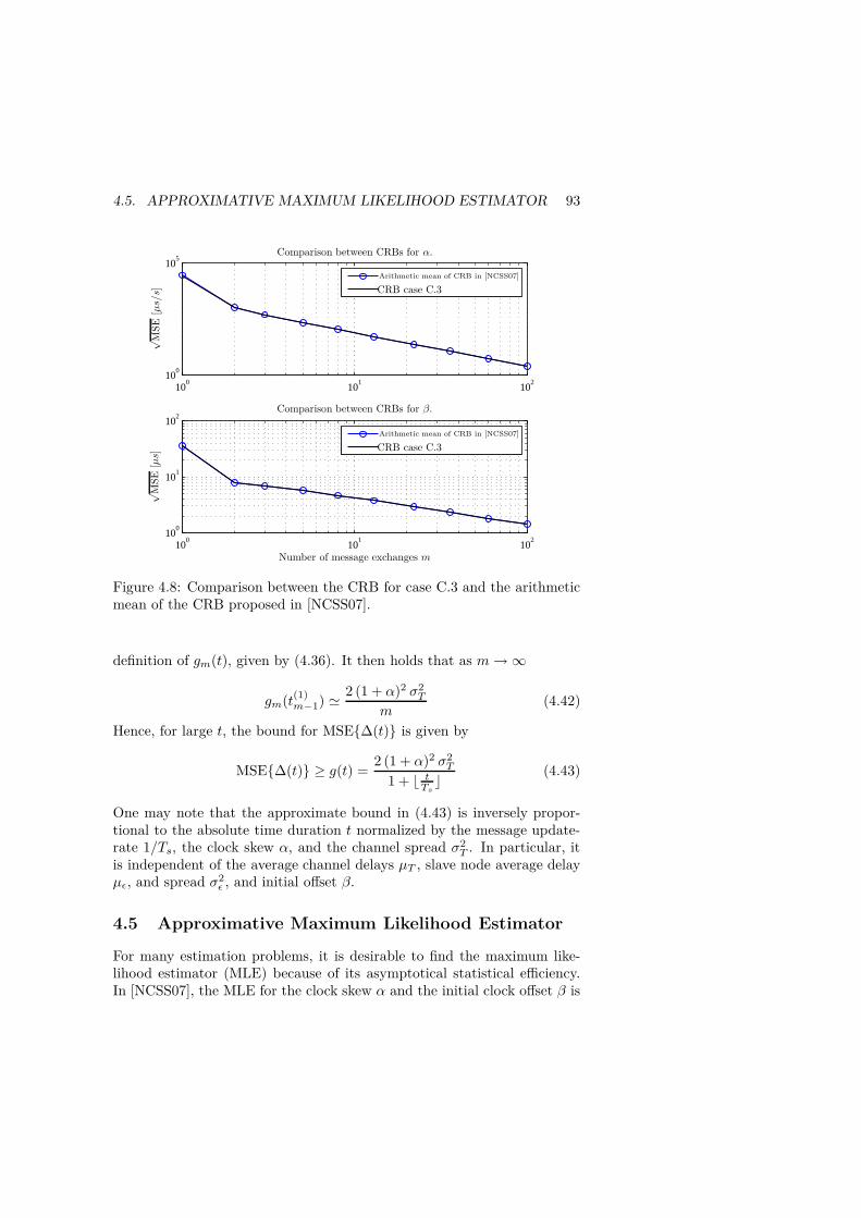
4.5. APPROXIMATIVE MAXIMUM LIKELIHOOD ESTIMATOR 93
100
101
102
100
105
100
101
102
100
101
102
Comparison between CRBs for α.
Comparison between CRBs for β.
Number of message exchanges m
√M
SE[µs/s]
√M
SE[µs]
CRB case C.3
CRB case C.3
Arithmetic mean of CRB in [NCSS07]
Arithmetic mean of CRB in [NCSS07]
Figure 4.8: Comparison between the CRB for case C.3 and the arithmeticmean of the CRB proposed in [NCSS07].
definition of gm(t), given by (4.36). It then holds that as m→∞
gm(t(1)m−1) ≃ 2 (1 + α)2 σ2
T
m(4.42)
Hence, for large t, the bound for MSE∆(t) is given by
MSE∆(t) ≥ g(t) =2 (1 + α)2 σ2
T
1 + ⌊ tTs ⌋(4.43)
One may note that the approximate bound in (4.43) is inversely propor-tional to the absolute time duration t normalized by the message update-rate 1/Ts, the clock skew α, and the channel spread σ2
T . In particular, itis independent of the average channel delays µT , slave node average delayµǫ, and spread σ2
ǫ , and initial offset β.
4.5 Approximative Maximum Likelihood Estimator
For many estimation problems, it is desirable to find the maximum like-lihood estimator (MLE) because of its asymptotical statistical efficiency.In [NCSS07], the MLE for the clock skew α and the initial clock offset β is
94 CHAPTER 4. SYNCHRONIZATION BY MESSAGE EXCHANGES
derived assuming the statistics of the delays to be known. However, whenthe statistics of the delays are unknown the estimation problem becomeshighly nonlinear [NCSS07]. Therefore, an AMLE for the clock skew α andthe initial clock offset β is proposed. The proposed AMLE is independentof the nuisance parameters (i.e., the delays statistics), and has a complexityequivalent to solving a linear least squares problem. Further, it is shownthat asymptotically the AMLE is nearly optimal, i.e., it nearly obtains theCRB.
4.5.1 Derivation
To derive the AMLE, introduce the artificial observation
zn = hT zn −t(1)n
2(4.44)
where h = 12
[1 1 −1
]T. Since zn is a linear combination of Gaussian-
distributed variables it will also be Gaussian-distributed. Further, the meanof zn is given by
Ezn = hT un(θ)− t(1)n
2= α t(1)
n + β + κ1 (4.45)
and the variance by
σ2z = COVzn = hT R h =
σ2T
2+ κ2. (4.46)
where κ1 and κ2 are given by
κ1 = α(µT +
µǫ2
)(4.47)
and
κ2 = α
((1 + α)σ2
T +ασ2ǫ
4
). (4.48)
One should note that κ1 ∈ O(α) and κ2 ∈ O(α), where O(x) denotesterms such that |O(x)/x| is bounded when x → 0. Thus, since the clockskew α in general is in the order of 10−5 or less for a quartz crystal os-cillator [SFCC08], the artificial observation (4.44) can be approximatelydescribed as
zn ≈ α t(1)n + β + wn, (4.49)
where wn ∼ N (0, σ2T /2) and independent in between different time instants.
For the approximate observation model (4.49), it holds that the MLE for

4.5. APPROXIMATIVE MAXIMUM LIKELIHOOD ESTIMATOR 95
the clock skew α and initial clock offset β is given by the linear least squaresestimator. Hence, introduce
ym =[z0 . . . zm−1
]T,
1m =[
1 . . . 1]T,
tm =[t(1)0 . . . t
(1)m−1
]T,
θ′ =[α β
]T,
(4.50)
and
Ψ =[
tm 1m]. (4.51)
The MLE estimator of θ givenm observations originating from the approx-imated artificial observation model (4.49) is then given by [Kay93b]
θ′ = (ΨT Ψ)−1 ΨT ym. (4.52)
Since the estimator in (4.52) is derived based on an approximation of thetrue artificial observation in (4.44), the estimator is referred to as theAMLE. (For an interesting comparison with respect to the linear trendMLE in the case of wn being exponentially distributed, refer to [Tru01].)Before comparing the AMLE to the CRB derived in Section 4.4, it shouldbe noted that the estimate of the AMLE is biased, as analyzed later.
4.5.2 Performance
Denote the bias by δθ′, that is
δθ′ = Eθ′ − θ′ = κ1 (ΨT Ψ)−1 ΨT 1m =
[0κ1
]. (4.53)
Hence, the AMLE does not belong to the class of estimators for which theunbiased CRB provides a lower bound on the MSE. For the AMLE, theMSE matrix of the estimated parameter vector is given by
Πm = E(θ′ − θ′)(θ′ − θ′)T = σ2
z(ΨT Ψ)−1 + δθ′ δθ′T
=
(σ2T
2+ κ2
)[ 12(m3−m)T 2
s
−6(m2+m)Ts
−6(m2+m)Ts
4m−2m2+m
]
+
[0 00 κ2
1
].
(4.54)
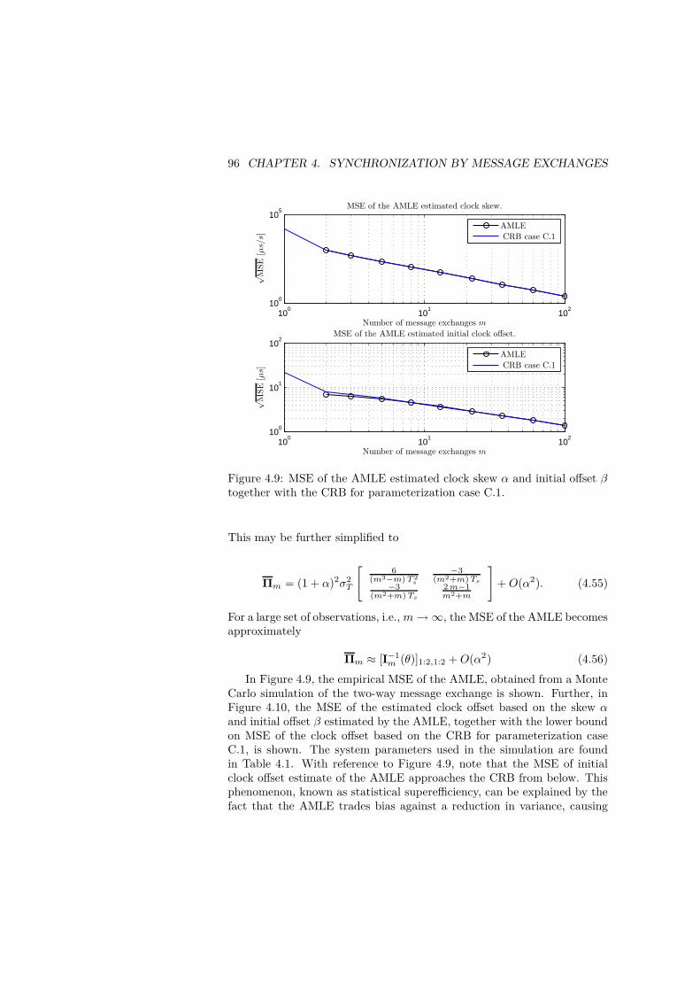
96 CHAPTER 4. SYNCHRONIZATION BY MESSAGE EXCHANGES
100
101
102
100
105
100
101
102
100
101
102
CRB case C.1
CRB case C.1
AMLE
AMLE
√M
SE[µs/s]
√M
SE[µs]
MSE of the AMLE estimated clock skew.
MSE of the AMLE estimated initial clock offset.
Number of message exchanges m
Number of message exchanges m
Figure 4.9: MSE of the AMLE estimated clock skew α and initial offset βtogether with the CRB for parameterization case C.1.
This may be further simplified to
Πm = (1 + α)2σ2T
[6
(m3−m)T 2s
−3(m2+m)Ts
−3(m2+m) Ts
2m−1m2+m
]+O(α2). (4.55)
For a large set of observations, i.e.,m→∞, the MSE of the AMLE becomesapproximately
Πm ≈ [I−1m (θ)]1:2,1:2 +O(α2) (4.56)
In Figure 4.9, the empirical MSE of the AMLE, obtained from a MonteCarlo simulation of the two-way message exchange is shown. Further, inFigure 4.10, the MSE of the estimated clock offset based on the skew αand initial offset β estimated by the AMLE, together with the lower boundon MSE of the clock offset based on the CRB for parameterization caseC.1, is shown. The system parameters used in the simulation are foundin Table 4.1. With reference to Figure 4.9, note that the MSE of initialclock offset estimate of the AMLE approaches the CRB from below. Thisphenomenon, known as statistical superefficiency, can be explained by thefact that the AMLE trades bias against a reduction in variance, causing

4.6. SIMULATION STUDY 97
0 0.2 0.4 0.6 0.8 110
0
101
MSE of the estimated clock offset.
MSE of the AMLE calculated clock offsetLower bound on the MSE of the clock offset
Time [s]
√M
SE[µs]
Figure 4.10: MSE of the estimated clock offset with skew α and initialoffset β estimated by the AMLE together with the lower bound on MSEof the clock offset based on the CRB for parameterization case C.1.
a reduction in MSE. For more details regarding statistically superefficientestimators, refer to [SO96, SM90].
4.6 Simulation Study
Consider the following offshore engineering scenario. An exploration ves-sel arrives at an oil drilling site with the intent to carry out work at theseabed using a remotely operated vehicle (ROV). On the seabed surround-ing the drill site, several sensor nodes for environmental monitoring havebeen deployed and their locations determined and mapped. The sensornodes act as slaves in the WSN used to position the ROV. Once at theintended operation site, the vessel anchors up to the seabed and puts theROV into the sea. Simultaneously, the exploration vessel sends out a com-mand to the nearby sensor nodes to get into ”positioning mode”, i.e., tolisten for the sound bursts sent out from the ROV and record their arrivaltimes and relay the information to the vessel. The vessel then uses thetime of arrival (TOA) information to determine the position of the ROV,and to calibrate its inertial navigation system. Refer to [CWCE06] for a

98 CHAPTER 4. SYNCHRONIZATION BY MESSAGE EXCHANGES
0100
200300
400500
0100
200300
400500
−100
−80
−60
−40
−20
0
20Vessel
NodeROV
z[m
]
x [m]y [m]
Illustration of the simulation scenario.
Figure 4.11: Illustration of the offshore engineering scenario used in thesimulation study.
survey on localization in underwater sensor networks. However, position-ing the ROV using the TOA information requires the clocks in the sensornetwork to be synchronized or the clock offsets of the nodes to be knownby the master node located at the vessel. To access this clock informationthe master node uses the two-way message exchange procedure describedin Section 4.3, in combination with the AMLE for the clock parameterestimation in Section 4.5.
With the above-described scenario as a basis, a Monte-Carlo simulationstudy was conducted to illustrate:
• The applicability of the two-way message exchange procedure to-gether with the AMLE to improve the accuracy of a WSN-basedpositioning system.
• How the bound on the MSE of the clock offset can be used to lowerbound the accuracy of the positioning system.
The study was conducted under the following assumptions. Four nodes,each in the corner of a square with the side 500 m, on the sea floor 100m below the average water surface level, were used in the positioning. See
4.6. SIMULATION STUDY 99
Figure 4.11 for an illustration of the scenario under study. The ship wasanchored so that on average it was located in the middle of the square,but due to waves its position randomly deviated according to a zero-meanGaussian distribution with covariance 42 · I3 m2; adding to the uncertain-ties in the transmission delays. Moreover, the ROV was moving in a circlewith a radius of 100 m and with its center at (250, 250, 90) and at a ve-locity of 2 m/s (a typical speed for ROVs [XHQHCD08]). The ROV wasequipped with a depth gauge and thus only the location in the horizontalplan was unknown. The slave nodes on the sea bed and the master nodeon the vessel communicated using acoustic signaling at a bit rate of 1250bits/s and with messages of a length of 56 bits, whereas the vessel and theROV were communicating using a wired connection, to allow high datathroughput for video information, etc. Refer to [APM05] for a discussionon underwater acoustic sensor networks and typical bit rates versus com-munication distances. Further, the nodes were assumed to be able to timestamp the message arrivals with an error drawn from a zero-mean Gaussiandistribution with a standard deviation proportional to the reciprocal of thebit rate. A study on underwater acoustic localization with many similar-ities to the above-described scenario is [XHQHCD08], but where a moreadvanced signal propagation model was employed. Moreover, the nodes’response time to a ”current clock state” request was modeled as Gaussiandistributed with a mean time of 50 ms and a standard deviation of 1 ms.The propagation speed of the sound in the water was assumed to be 1500m/s.
The bound on the MSE of the clock offset, derived in Section 4.4.4, canbe mapped into a bound on the MSE of the position error of the ROV. Todo so, let i (for i = 1, . . . , 4) denote the sensor node under consideration.The clock state of the node, when receiving the positioning pulse sent fromthe ROV, can then be described as
Csi (tirx) = tirx + ∆i(t
irx)
= hi(p) + titx + ∆i(ttx) + wi
+ α (hi(p) + wi)
≈ hi(p) + ttx + ∆i(ttx) + wi
(4.57)
where
hi(p) =‖ri − p‖vs
. (4.58)
Here, titx and tirx denote transmission and receiving time of the positionpulse, respectively. Further, wi denotes the stochastic error in the timestamping of the received burst, and is assumed zero-mean Gaussian withvariance σ2
w . Moreover, ri and p denotes the position of the ith node

100 CHAPTER 4. SYNCHRONIZATION BY MESSAGE EXCHANGES
500 1000 1500 2000 2500 3000 35001
1.5
2
2.5
3
3.5
MSE of the horizontal position error of the ROV.
Time [s]
√M
SE[m
]
Monte Carlo Simulation.CRB based bound.Monte Carlo Simulation, 360 message exchanges.CRB based bound, 360 message exchanges.Position error with perfect clock synchronization.
Figure 4.12: Monte Carlo and CRB based MSE of the horizontal positionerror of the ROV in the simulation study.
and the ROV, respectively. The constant vs is the speed of sound in thewater. Assuming that the TOA algorithm uses these four observations to-gether with the current clock offset estimates, i.e., ∆i(ttx) = αittx + βifor i = 1, . . . , 4, to calculate a position estimate p using a nonlinear leastsquare approach. Then, the MSE of the observations becomes approxi-mately [FB98]
MSE(p− p) ≈ H†(Υ∆ + σ2wI3)(H†)T (4.59)
where
H =
∇h1(p)∇h2(p)∇h3(p)∇h4(p)
. (4.60)
Here, ∇ and † denote the gradient and matrix pseudo inverse, respectively.Further, Υ∆ is the MSE matrix of the clock offset estimates. Assumingthe clock offset estimates to be uncorrelated and using the lower bound forthe MSE of the clock offset derived in Section 4.4.4, a bound on the MSEof the positioning error of the ROV can be calculated.

4.7. CONCLUSIONS 101
The by Monte Carlo simulation calculated MSE of the position esti-mates of the ROV is shown in Figure 4.12. Also shown is the MSE of theposition estimates for the case when the clock synchronization was stoppedafter 1800 s (i.e., after 360 message exchanges with each node) and there-after the clock offset was predicted using the estimated clock parameters.Moreover, the lower bound on the MSE of the position estimates, basedon (4.59) and (4.43), has been evaluated with the same parameters as thesimulation scenario and is also shown in Figure 4.12.
The improvements in position accuracy owing to the time synchroniza-tion are evident from the results in Figure 4.12. After 3600 s (i.e., 720message exchanges with each node), the effect of the clock synchroniza-tion errors is negligible when compared with the other error sources inthe trilateration of the ROV, the position accuracy being close to the ac-curacy achievable with perfect clock synchronization. The results of thesimulation in which the clock synchronization was stopped after 360 mes-sage exchanges (i.e., 1800 s) show the benefit of estimating the clock skew.Even though the synchronization has been stopped, the offset of the slavenode clocks can be predicted and the position error growth thereby reduced.Moreover, the bounds on the position accuracy for the two simulation casesagree well with the results from the Monte Carlo simulations, illustratingthe application of the derived CRB as a tool for accessing the impact ofthe time synchronization at a system level.
In summary, to illustrate the application of the derived CRB, beyondbeing a versatile tool for accessing the theoretical limitations of the two-way message exchange clock synchronization, a simulation study on TOApositioning in an underwater WSN was conducted. In the study, the two-way message exchange together with the AMLE was used to synchronizethe sensor nodes used in the TOA positioning of an ROV, illustrating therelationship between the estimation accuracy of the clock parameters andthe accuracy at which the ROV could be positioned. Moreover, the lowerbound on the MSE of the clock offset was mapped into a lower bound onthe accuracy of the TOA positioning algorithm.
4.7 Conclusions
The accuracy with which the clock offset between a master and a slave nodein a sensor network can be estimated using a two-way message exchangebetween the nodes has been investigated. The study has been conductedunder a set of assumptions. The most important assumptions being: theclocks can be described by linear models (including affine mappings), the(wireless) communication channel is symmetric, and the communicationlatency within the channel can be described as Gaussian. Under these con-ditions, the CRB for the estimation of the clock skew and initial clock offset

102 CHAPTER 4. SYNCHRONIZATION BY MESSAGE EXCHANGES
were derived for four different scenarios (distinguished by the set of nui-sance parameters), reflecting different levels of prior knowledge concerningthe system parameters. The asymptotic CRB is derived as well and shownto be the same for the considered scenarios. For large sample sets the lowerbound on the variance of the skew is inversely proportional to the cube ofthe number of message exchanges, and the variance of the initial offset isinversely proportional to the number of message exchanges, i.e., it is easierto estimate the clock skew than the initial clock offset.
Further, the derived CRB for the clock skew and initial clock offset wasmapped into a lower bound on the MSE of the clock offset. Asymptotically,the lower bound on the MSE is inversely proportional to the absolute timeduration t normalized by the message update-rate 1/Ts, the clock skew,and the channel spread. In particular, it is independent of the averagechannel delays, slave node average delay and spread, and the initial clockoffset.
By creating a set of artificial observations through linear combinationsof the observations originally obtained from the two-way message exchange,a low-complexity AMLE was derived. The estimator’s performance wasexamined both theoretically and through numerical evaluations, and com-pared with the derived CRB. Asymptotically, the AMLE was shown to benearly optimal, i.e., it nearly obtains the CRB.

4.A. FIM ELEMENTS 103
4.A FIM Elements
In case C.2 the FIM is given by are given by the FIM for case C.1 plus thefollowing nonzero elements
[Im(θ)]1,3 = [Im(θ)]3,1 = − µǫm
(1 + α)σ2T
, (4.61)
[Im(θ)]1,4 = [Im(θ)]4,1 =m
(1 + α)σ2T
, (4.62)
[Im(θ)]3,3 =2m
σ2T
, and [Im(θ)]4,4 =m
σ4T
. (4.63)
In case C.3 the FIM is given by are given by the FIM for case C.1 plus thefollowing nonzero elements
[Im(θ)]1,3 = [Im(θ)]3,1 =µǫm
(1 + α)σ2ǫ
, (4.64)
[Im(θ)]1,4 = [Im(θ)]4,1 =m
(1 + α)σ2ǫ
, (4.65)
[Im(θ)]3,3 =m
σ2ǫ
, and [Im(θ)]4,4 =m
2 σ4ǫ
. (4.66)
In case C.4 the FIM is given by FIM for case C.2 plus the following nonzeroelements
[Im(θ)]1,5 = [Im(θ)]5,1 =µǫm
(1 + α)σ2ǫ
, (4.67)
[Im(θ)]1,6 = [Im(θ)]6,1 =m
(1 + α)σ2ǫ
, (4.68)
[Im(θ)]5,5 =m
σ2ǫ
, and [Im(θ)]6,6 =m
2 σ4ǫ
. (4.69)
4.B Polynomial Functions in the CRB Expressions
The polynomial functions in the expression for the CRB in (4.28)–(4.30)reads
c1(m) = 3m (10 σ2T σ
2ǫ + 2 σ4
ǫ + 2µ2ǫ σ
2T + µ2
ǫ σ2ǫ ), (4.70)
c2(m) = 6m (4 σ2T σ
2ǫ + µ2
ǫ σ2T + σ4
ǫ ), (4.71)

104 CHAPTER 4. SYNCHRONIZATION BY MESSAGE EXCHANGES
c3(m) = 3m(6 σ2T + 2σ2
ǫ + µ2ǫ )σ
2ǫ , (4.72)
c4(m) = 6m(2 σ2T + σ2
ǫ )σ2ǫ , (4.73)
d1(m) = T 2s + 6µ2
T + 15 σ2T + 6µT ((m− 1)Ts + µǫ)
+ 3 ((m− 1)Ts µǫ + µ2ǫ (1 +
σ2T
σ2ǫ
) + σ2ǫ ),
(4.74)
d2(m) = T 2s + 12σ2
T +3µ2ǫσ
2T
σ2ǫ
+ 3σ2ǫ
+3
2(2µT + µǫ) (2 (m− 1)Ts + 2µT + µǫ) ,
(4.75)
d3(m) = T 2s + 6µ2
T + 6µT ((m− 1)Ts + µǫ)
+ 3µǫ ((m− 1)Ts + µǫ) + 9 σ2T + 3 σ2
ǫ ,(4.76)
and
d4(m) = T 2s + 6 σ2
T + 3σ2ǫ
+3
2(2µT + µǫ) (2(m− 1)Ts + 2µT + µǫ) .
(4.77)
4.C Proofs of the Inequalities
Proofs of the inequalities in (4.37) and (4.38), used in the derivation of thelower bound for the clock offset.
4.C.1 First Inequality
To show the inequality
gm(ξ + t(1)m−1) ≥ gm(t
(1)m−1), ∀ξ ≥ 0 : m ∈ Ωm (4.78)
where Ωm = m |m ∈ N and m ≥ (2µT + µǫ)/Ts + 1, let ν1(ξ) = gm(ξ +
t(1)m−1)−gm(t
(1)m−1). From the definition of gm(t) in (4.36) it then holds that
ν1(ξ) = [Im]1,1ξ2 + 2
([Im]1,2 + t
(1)m−1 [Im]1,1
)ξ, (4.79)

4.C. PROOFS OF THE INEQUALITIES 105
which can be identified as a convex quadratic polynomial function. Further,its roots are located at ξ1 = 0 and
ξ2 = −2([Im]1,2/[Im]1,1 + t(1)m−1)
= (1−m)Ts + 2µT + µǫ,(4.80)
and thus ν1(ξ) ≥ 0, ∀ξ ≥ max(ξ1, ξ2). Hence, given that m ≥ (2µT +µǫ)/Ts + 1, then ξ2 ≤ 0 and ν1(ξ) ≥ 0, ∀ξ ≥ 0, from which the inequalityin (4.78) follows directly.
4.C.2 Second Inequality
To show the inequality gm−1(t) ≥ gm(t), ∀t, let ν2(t) = gm−1(t) − gm(t).From the definition of gm(t) in (4.36) it then holds that
ν2(t) = xT (t)[I−1m−1 − I−1
m ]1:2,1:2 x(t)
= xT (t)[I−1m−1 − (Im−1 + Jm)−1]1:2,1:2 x(t)
= xT (t)[I−1m−1(Jm + Im−1) I−1
m−1]1:2,1:2 x(t)
≥ 0,
(4.81)
where Im ≡ Im(θ) and Jm ≡ Jm(θ). In the second equality the matrixinversion lemma was used and the final inequality follows from the fact thatJm(θ) and Im−1(θ) are positive semidefinite symmetric matrices. From(4.81) the inequality in follows directly.

Chapter 5
Zero-Velocity Detection in
Pedestrian Navigation Systems
5.1 Introduction
The integrative nature of the inertial navigation system (INS) conveys thatits sensor errors give rise to a position error that grows proportional to thecube of the system’s operation time [ESN07]. Therefore, with the perfor-mance of the low-cost inertial sensors currently available, free inertial navi-gation is only feasible for time periods in the range of a few seconds [ESN07,SH09a, RSV07]. However, the devastating cubic error growth can be bro-ken by imposing constraints on the navigation solution using informationabout the system dynamics [ESN07, SH09a, GC07, DSNDW01, Fox05]. Atype of information commonly used for this purpose is knowledge aboutthe time epochs when the system is in a stationary phase, i.e., when thesystem has a constant position and attitude. This method is referred to aszero-velocity updates. A conceptual description of a zero-velocity updateconstrained INS is shown in Figure 5.1.
The use of zero-velocity updates is especially appealing for constrainingfoot-mounted INSs, as during ordinary gait, the foot returns to a "station-ary" state on a regular base [Sab06]. Indeed, this idea has been success-fully applied [GL08, OB07], resulting in systems where the position errorgrows proportionally with respect to the number of steps taken by theuser [OB07, Fox05]. For details on the benefits of zero-velocity updates,one can refer to [GBYT02] and the references therein. However, the use ofzero-velocity updates requires identification of the time epochs when the in-ertial measurement unit (IMU) is stationary [GL08]. Accordingly, a rangeof detectors have been proposed for detecting the stationary epochs on thebasis of the inertial sensor data [VBdV+96, GLC06, KLC08, GL08, KR08,FZGB09, OB07]. Moreover, within the field of gait analysis in biomedicine,
107
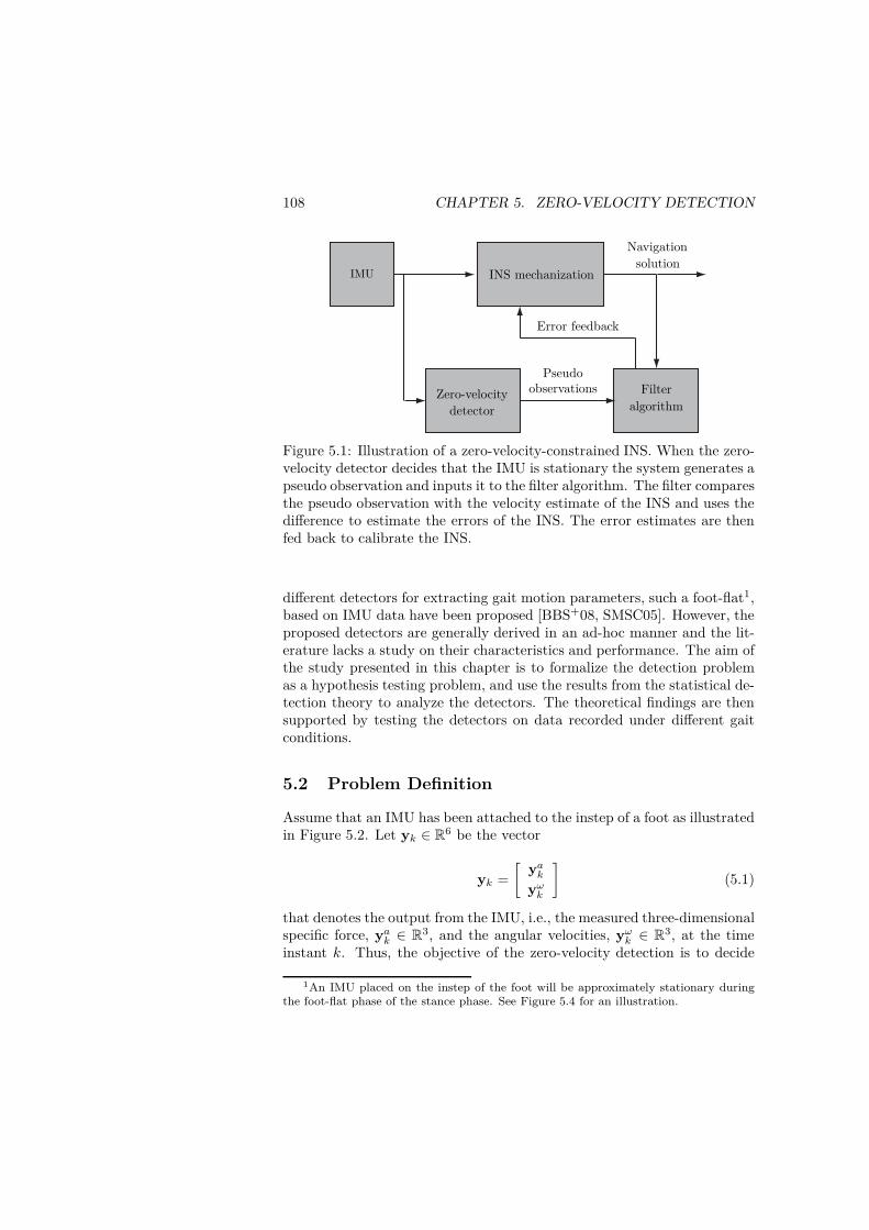
108 CHAPTER 5. ZERO-VELOCITY DETECTION
IMU
Zero-velocitydetector
INS mechanization
Pseudoobservations Filter
algorithm
Navigationsolution
Error feedback
Figure 5.1: Illustration of a zero-velocity-constrained INS. When the zero-velocity detector decides that the IMU is stationary the system generates apseudo observation and inputs it to the filter algorithm. The filter comparesthe pseudo observation with the velocity estimate of the INS and uses thedifference to estimate the errors of the INS. The error estimates are thenfed back to calibrate the INS.
different detectors for extracting gait motion parameters, such a foot-flat1,based on IMU data have been proposed [BBS+08, SMSC05]. However, theproposed detectors are generally derived in an ad-hoc manner and the lit-erature lacks a study on their characteristics and performance. The aim ofthe study presented in this chapter is to formalize the detection problemas a hypothesis testing problem, and use the results from the statistical de-tection theory to analyze the detectors. The theoretical findings are thensupported by testing the detectors on data recorded under different gaitconditions.
5.2 Problem Definition
Assume that an IMU has been attached to the instep of a foot as illustratedin Figure 5.2. Let yk ∈ R6 be the vector
yk =
[yakyωk
](5.1)
that denotes the output from the IMU, i.e., the measured three-dimensionalspecific force, yak ∈ R3, and the angular velocities, yωk ∈ R3, at the timeinstant k. Thus, the objective of the zero-velocity detection is to decide
1An IMU placed on the instep of the foot will be approximately stationary duringthe foot-flat phase of the stance phase. See Figure 5.4 for an illustration.

5.2. PROBLEM DEFINITION 109
IMU
FSR FSR
x-axis
y-axis
z-axis
Figure 5.2: Illustration of the on the instep-mounted IMU and the force-sensitive resistors (FSRs) used in the reference system.
whether, during a time epoch consisting of N observations2 between thetime instants n and n+N − 1, the IMU is moving or stationary, given themeasurement sequence
zn , ykn+N−1k=n . (5.2)
Further, the decisions should be made in such a way that the probability ofdeciding that the IMU is stationary when it is not should be kept low. Thisis owing to the ruinous effect of imposing an erroneous constraint on thenavigation solution. However, as imposing the constraints when it holdstrue is the key to break the cubic error drift, the probability of detectingthe stationary events should be maximized given a certain error decisionprobability.
Mathematically, we can formalize the detection problem as a binaryhypothesis testing problem, where the detector can choose between thetwo hypotheses H0 and H1, defined as
H0 : IMU is moving
H1 : IMU is stationary(5.3)
The detector performance is then specified by the false-alarm probabil-ity PFA = PrH1|H0 (i.e., the probability of deciding on the hypothesisH1 when hypothesis H0 is true) and the probability of detection PD =PrH1|H1 (i.e., the probability of deciding hypothesis H1 when it is
2The choice on the number of observations N will depend upon the sample rate ofthe system and the length of the time epochs for which the IMU is assumed stationary.
110 CHAPTER 5. ZERO-VELOCITY DETECTION
true). Further, Neyman-Pearson (NP) theorem tells us how to choose be-tween the two hypotheses to maximize PD for a given PFA. Let p(zn;H0)and p(zn;H1) denote the probability density functions (PDFs) of the ob-servations for the two hypotheses. Thus, the NP theorem then statesthat [Kay93a]
Theorem 1 (Neyman-Pearson) To maximize PD for PFA = α decideon H1 if
L(zn) =p(zn;H1)
p(zn;H0)> γ, (5.4)
where the threshold γ is determined from
PFA =
∫
zn:L(zn)>γ
p(zn;H0) = α. (5.5)
The function L(zn) in (5.4) is referred to as the likelihood ratio, as foreach value zn, it indicates the likelihood of the H1 hypothesis versus theH0 hypothesis. Moreover, the test in (5.4) is referred to as the likelihoodratio test (LRT). Clearly, the LRT require complete knowledge about thePDFs of the observations for the two hypotheses. Therefore, as the PDFsof the observations are mostly only partly known, we often have to chooseapproximate hypothesis tests methods.
5.3 Signal and Sensor Model
The PDFs of the observed data depends both upon the true signal and thedistortion introduced to the signal by the sensors. Hence, to find the PDFsof the observations, we must specify a signal and sensor model. The choiceof models should be balanced between the mathematical tractability andrealistic description of the signal and the sensor.
5.3.1 Sensor Model
For IMU sensors, there is a vast amount of models with various complex-ities [SH06a, GWA07, Rog03, Sab05]. We will restrict our analysis to thecase when the sensor output may be described as
yk = sk(θ) + vk, (5.6)
where
sk(θ) =
[sak(θ)sωk (θ)
], (5.7)

5.3. SIGNAL AND SENSOR MODEL 111
and
vk =
[vakvωk
]. (5.8)
Here, sak(θ) ∈ R3 and sωk (θ) ∈ R3 denote the IMU-sensed specific forceand angular velocity, respectively. Further, θ denotes the set of unknownparameters needed to describe the signals. Moreover, vak ∈ R3 and vωk ∈ R3
denote the noise associated with the accelerometer and gyroscope sensorassembly, respectively. We will assume that the noise is i.i.d., zero-mean,Gaussian with covariance matrix
C = Evk vTk =
[σ2a I3 03
03 σ2ω I3
], (5.9)
where I3 (03) denotes an identity (zero) matrix of size 3× 3. Further, E·denotes the expectation operation, and σ2
a ∈ R1 and σ2ω ∈ R1 denote the
accelerometer and gyroscope noise variance, respectively.
5.3.2 Signal Model
Modeling the specific force and angular velocities, i.e., sk(θ), experiencedby the foot-mounted IMU under the hypothesis H0 (that the IMU is inmotion) in a consistent way that reflects a diverse set of gaits, is difficult.However, under hypothesis H1 (that the IMU is stationary), the followingconditions hold true (neglecting the effect of the earth rotation rate):
• The only force sensed by the accelerometers assembly is the gravita-tion acceleration, whose magnitude is known.
• The attitude of the IMU is constant, i.e., the angular velocity expe-rienced by the IMU is zero.
In other words, mathematically, for the two hypotheses, the signal fulfillsthe conditions
H0 : sak(θ) 6= gun or sωk (θ) 6= 03,1 ∀k ∈ Ωn
H1 : sak(θ) = gun and sωk (θ) = 03,1 ∀k ∈ Ωn(5.10)
Here un ∈ Ωu, where Ωu = u ∈ R3 : ‖u‖ = 1 and g ∈ R1 is themagnitude of the local gravity vector. Moreover, ‖u‖ =
√uT u where T
denotes the transpose operation and Ωn = ℓ ∈ N : n ≤ ℓ < N−1. Hence,for the two hypothesis the unknown parameters of the signal are
H0 : θ ≡ skn+N−1k=n
H1 : θ ≡ un.(5.11)

112 CHAPTER 5. ZERO-VELOCITY DETECTION
That is, under H0, the signal sk(θ) is completely unknown, whereas underH1, only the direction of the specific force vector is unknown. In Figure 5.4,the output from an instep-mounted IMU during the stance phase of the gaitis shown.
5.3.3 PDFs of Observations
Owing to the lack of knowledge about the signal parameters θ, we cannotcompletely specify the PDFs of the observations under the two hypotheses.However, with the sensor model specified by (5.6)–(5.9), the measurementsmay originate from the family of PDFs, which are given by (for i = 0, 1)
p(zn; θ,Hi) =∏
k∈Ωn
p(yk; θ,Hi)
=∏
k∈Ωn
p(yak; θ,Hi) p(yωk ; θ,Hi),(5.12)
where
p(yak; θ,Hi) =1
(2πσ2a)
3/2exp(− 1
2σ2a
‖yak − sak(θ)‖2), (5.13)
and
p(yωk ; θ,Hi) =1
(2πσ2ω)3/2
exp(− 1
2σ2ω
‖yωk − sωk (θ)‖2). (5.14)
5.4 Generalized Likelihood Ratio Test
As the PDFs of the observations under the two hypotheses are parameter-ized by a set of, to us, unknown parameters θ, i.e., the (partly) unknownsignal sk(θ), we cannot apply the LRT in (5.4). However, by substitutingthe unknown parameters with their maximum likelihood estimates (MLEs),we can derive a GLRT. The GLRT decides on H1, if
LG(zn) =p(zn; θ1,H1)
p(zn; θ0,H0)> γ, (5.15)
where θ1 is the MLE of the unknown parameters assuming H1 is true, andθ0 is the MLE of the unknown parameters assuming H0 is true.
The MLE is obtained by maximizing (5.12) with respect to the unknownparameters. In our case, under H0, the signal is completely unknown andθ0 = ykn+N−1
k=n . Thus,

5.4. GENERALIZED LIKELIHOOD RATIO TEST 113
p(zn; θ0,H0) =1
(2πσ2a)
3N/2· 1
(2πσ2ω)3N/2
. (5.16)
Under H1 we can obtain the MLE of the unknown signal parameter un bymaximizing
p(zn; un,H1) =1
(2πσ2a)
3N/2exp(− 1
2σ2a
∑
k∈Ωn
‖yak − gun‖2)
· 1
(2πσ2ω)3N/2
exp(− 1
2σ2ω
∑
k∈Ωn
‖yωk ‖2)
(5.17)
with respect to un ∈ Ωu. That is,
un = argmaxu∈Ωu
(p(zn; u,H1)
)
= argminu∈Ωu
( ∑
k∈Ωn
‖yak − gu‖2)
= argminu∈Ωu
( ∑
k∈Ωn
‖yak‖2 − 2 (yak)Tu + g2‖u‖2
)
= argmaxu∈Ωu
((yan)
Tu)
=yan‖yan‖
,
(5.18)
where
yan =1
N
∑
k∈Ωn
yak. (5.19)
The last equality in (5.18) follows from Cauchy’s Schwarz’ inequality: aTb ≤‖a‖‖b‖, with equality observed only if a = cb; c being a real constant.Substituting un into (5.17) yields
p(zn; θ1,H1) = p(zn; un,H1)
=1
(2πσ2a)
3N/2· 1
(2πσ2ω)3N/2
· exp(− 1
2σ2a
∑
k∈Ωn
‖yak − gyan‖yan‖
‖2)
· exp(− 1
2σ2ω
∑
k∈Ωn
‖yωk ‖2).
(5.20)
Next, if we combine (5.15), (5.16), and (5.20), the GLRT becomes: decideon H1 if
114 CHAPTER 5. ZERO-VELOCITY DETECTION
LG(zn) = exp(− 1
2σ2a
∑
k∈Ωn
‖yak − gyan‖yan‖
‖2)
· exp(− 1
2σ2ω
∑
k∈Ωn
‖yωk ‖2) > γ.
(5.21)
We may further simplify the test with respect to the fact that the logarithmis monotonically increasing. To do so, let
T (zn) = − 2
NlnLG(zn). (5.22)
We can then state the GLRT as: choose H1 if
T (zn) =1
N
∑
k∈Ωn
(1
σ2a
‖yak − gyan‖yan‖
‖2 +1
σ2ω
‖yωk ‖2)< γ′. (5.23)
We can interpret this as follows: if the mean square error of fitting a vectorof magnitude g, with the direction of the average specific force vector to theaccelerometer data in combination with the energy in the gyroscope signal,each weighted by quality of the measurements, falls bellow the threshold γ′,the GLRT chooses the hypothesis that the IMU is stationary. In Figure 5.3,the test statistics T (zn) based upon the data from a foot-mounted IMU,sampled at 30 Hz, during leveled ground, forward gait, is shown. Figure 5.3also shows the time moments n when all the data samples in zn originatefrom a stationary phase according to our reference system. Details on thereference system are presented in Section 5.5.
5.4.1 Acceleration Moving Variance Detector
A detector proposed in the literature to detect when the IMU is stationary,is the acceleration moving variance detector [VBdV+96, GLC06, KLC08,GL08]. The moving variance detector is solely based upon the accelerom-eter data and is defined as follows: decide on H1 if
Tv(zan) =
1
N
∑
k∈Ωn
‖yak − yan‖2 < γv, (5.24)
where
zan , yakn+N−1k=n . (5.25)
We can derive the acceleration moving variance detector within the GLRTframe work with respect to the fact that the orientation of the accelerometer
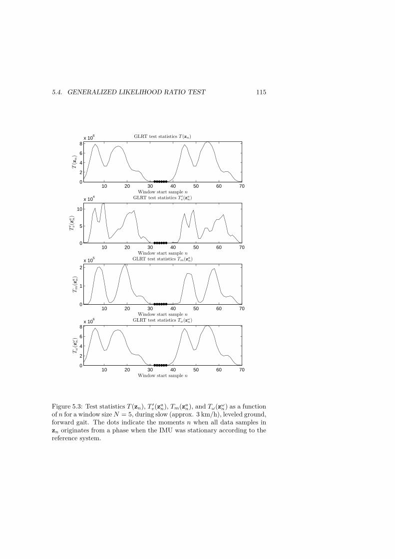
5.4. GENERALIZED LIKELIHOOD RATIO TEST 115
10 20 30 40 50 60 700
2
4
6
8x 10
6
10 20 30 40 50 60 700
5
10
x 104
10 20 30 40 50 60 700
1
2
x 105
10 20 30 40 50 60 700
2
4
6
8x 10
6
GLRT test statistics T (zn)
T(zn)
GLRT test statistics T ′v(zan)
T′ v(za n)
GLRT test statistics Tm(zan)
Tm
(za n)
GLRT test statistics Tω(zωn)
Tω(zω n
)
Window start sample n
Window start sample n
Window start sample n
Window start sample n
Figure 5.3: Test statistics T (zn), T ′v(zan), Tm(zan), and Tω(zωn) as a function
of n for a window sizeN = 5, during slow (approx. 3 km/h), leveled ground,forward gait. The dots indicate the moments n when all data samples inzn originates from a phase when the IMU was stationary according to thereference system.

116 CHAPTER 5. ZERO-VELOCITY DETECTION
assembly is constant when the IMU is stationary, but neglecting the factthat the magnitude of the specific force vector is equal to g. To derivethe test, let us assume that under the two hypotheses, the signal from theaccelerometer cluster fulfills the conditions
H0 : sak(θv) 6= sa ∀k ∈ Ωn
H1 : sak(θv) = sa ∀k ∈ Ωn(5.26)
where sa ∈ R3 is unknown. Hence, the unknown parameters needed todescribe the signal under the two hypotheses are
H0 : θv ≡ sakn+N−1k=n
H1 : θv ≡ sa(5.27)
and thus, the family of PDFs describing the accelerometer observations isgiven by (for i = 0, 1)
p(zan; θv,Hi) =∏
k∈Ωn
p(yak, θv,Hi). (5.28)
With this information in hand, under H0, the MLE θ0v = yakn+N−1k=n .
Thus,
p(zan; θ0v,H0) =1
(2πσ2a)
3N/2. (5.29)
Further, the MLE of the unknown parameters under H1 are given by
sa = argmaxs
(p(zan; s,H1)
)
= argmins
( ∑
k∈Ωn
‖yak − s‖2)
= yan.(5.30)
Therefore,
p(zan; θ1v,H1) = p(zan; sa,H1) =1
(2πσ2a)
3N/2
· exp(− 1
2σ2a
∑
k∈Ωn
‖yak − yan‖2).(5.31)
Hence, if we combine (5.15), (5.22), (5.29), and (5.31), the GLRT becomesas follows: choose H1 if

5.4. GENERALIZED LIKELIHOOD RATIO TEST 117
T ′v(zan) = − 2
Nlnp(zan; θ1v,H1)
p(zan; θ0v,H0)
=1
σ2aN
∑
k∈Ωn
‖yak − yan‖2 < γ′v,(5.32)
which is equivalent to the test in (5.24). In Figure 5.3, the test statisticsT ′v(z
an) based upon the data from a foot-mounted IMU, sampled at 30 Hz,
during leveled ground, forward gait, is shown. Figure 5.3 also shows thetime moments n when all the data samples in zan originate from a stationaryphase according to the reference system.
5.4.2 Acceleration Magnitude Detector
The acceleration magnitude detector is another detector proposed in theliterature [GLC06, GL08, KR08], and is often used as a supplement to themoving variance detector. The acceleration magnitude detector checks ifthe measured specific force vector is close to g, and if that is the case,concludes that the IMU is stationary. We can derive this type of detectorwithin the GLRT framework based on the fact that the magnitude of thespecific force vector is g when the IMU is stationary, but neglecting the factthat the direction of the vector should be constant. To derive the test, letus assume that under the two hypotheses, the signal from the accelerometercluster fulfills the conditions
H0 : sak(θm) 6= guk ∀k ∈ Ωn
H1 : sak(θm) = guk ∀k ∈ Ωn(5.33)
where uk ∈ Ωu. Hence, the unknown parameters needed to describe thesignal under the two hypotheses are
H0 : θm ≡ sakn+N−1k=n
H1 : θm ≡ ukn+N−1k=n
(5.34)
Again, the family of PDFs describing the accelerometer observations isgiven by (5.28); however, now the unknown parameters are those in (5.34).UnderH0, when the signal is completely unknown, the MLE θ0m = yakn+N−1
k=n
and p(zan; θ0m,H0) is given by (5.29). Further, under H1, the MLEs of the
unknown parameters are given by (for ℓ = n, . . . , N + n− 1)
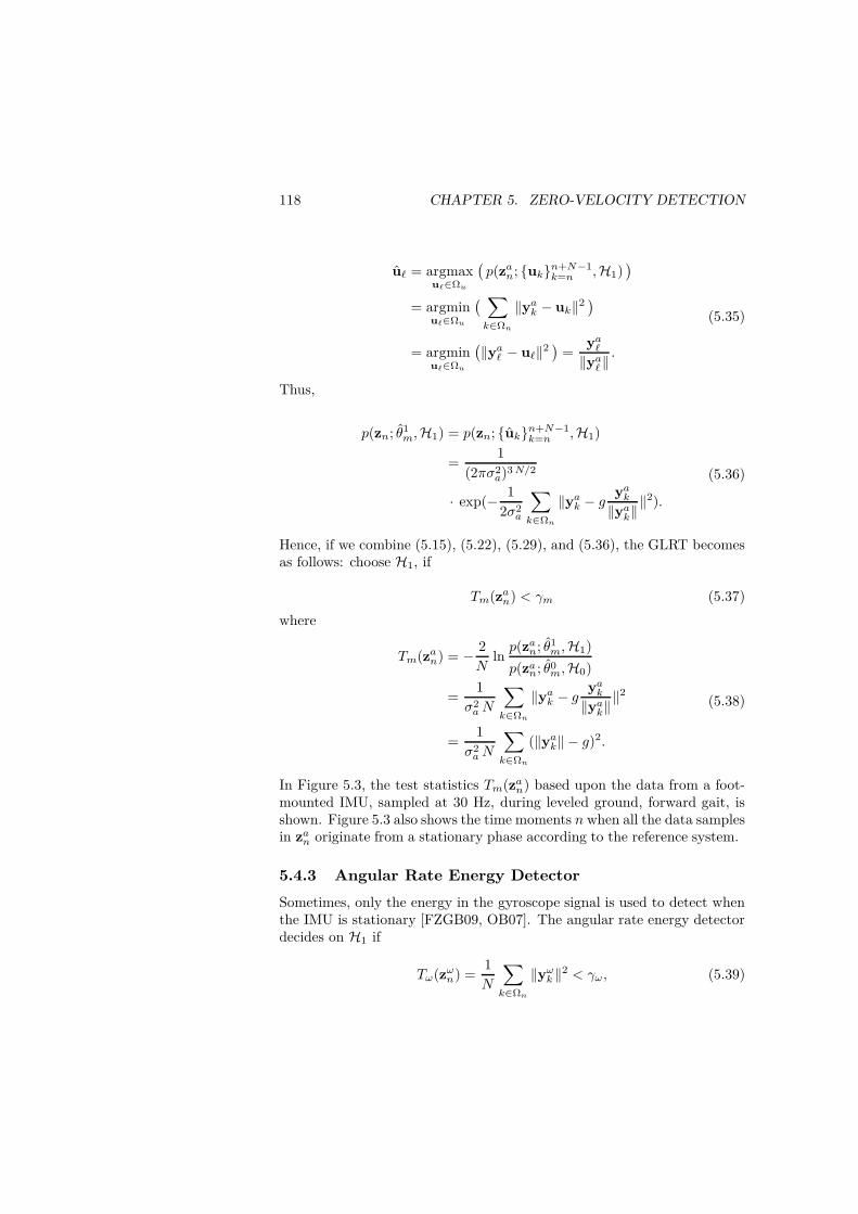
118 CHAPTER 5. ZERO-VELOCITY DETECTION
uℓ = argmaxuℓ∈Ωu
(p(zan; ukn+N−1
k=n ,H1))
= argminuℓ∈Ωu
( ∑
k∈Ωn
‖yak − uk‖2)
= argminuℓ∈Ωu
(‖yaℓ − uℓ‖2
)=
yaℓ‖yaℓ‖.
(5.35)
Thus,
p(zn; θ1m,H1) = p(zn; ukn+N−1k=n ,H1)
=1
(2πσ2a)
3N/2
· exp(− 1
2σ2a
∑
k∈Ωn
‖yak − gyak‖yak‖‖2).
(5.36)
Hence, if we combine (5.15), (5.22), (5.29), and (5.36), the GLRT becomesas follows: choose H1, if
Tm(zan) < γm (5.37)
where
Tm(zan) = − 2
Nlnp(zan; θ
1m,H1)
p(zan; θ0m,H0)
=1
σ2aN
∑
k∈Ωn
‖yak − gyak‖yak‖‖2
=1
σ2aN
∑
k∈Ωn
(‖yak‖ − g)2.
(5.38)
In Figure 5.3, the test statistics Tm(zan) based upon the data from a foot-mounted IMU, sampled at 30 Hz, during leveled ground, forward gait, isshown. Figure 5.3 also shows the time moments n when all the data samplesin zan originate from a stationary phase according to the reference system.
5.4.3 Angular Rate Energy Detector
Sometimes, only the energy in the gyroscope signal is used to detect whenthe IMU is stationary [FZGB09, OB07]. The angular rate energy detectordecides on H1 if
Tω(zωn) =1
N
∑
k∈Ωn
‖yωk ‖2 < γω, (5.39)
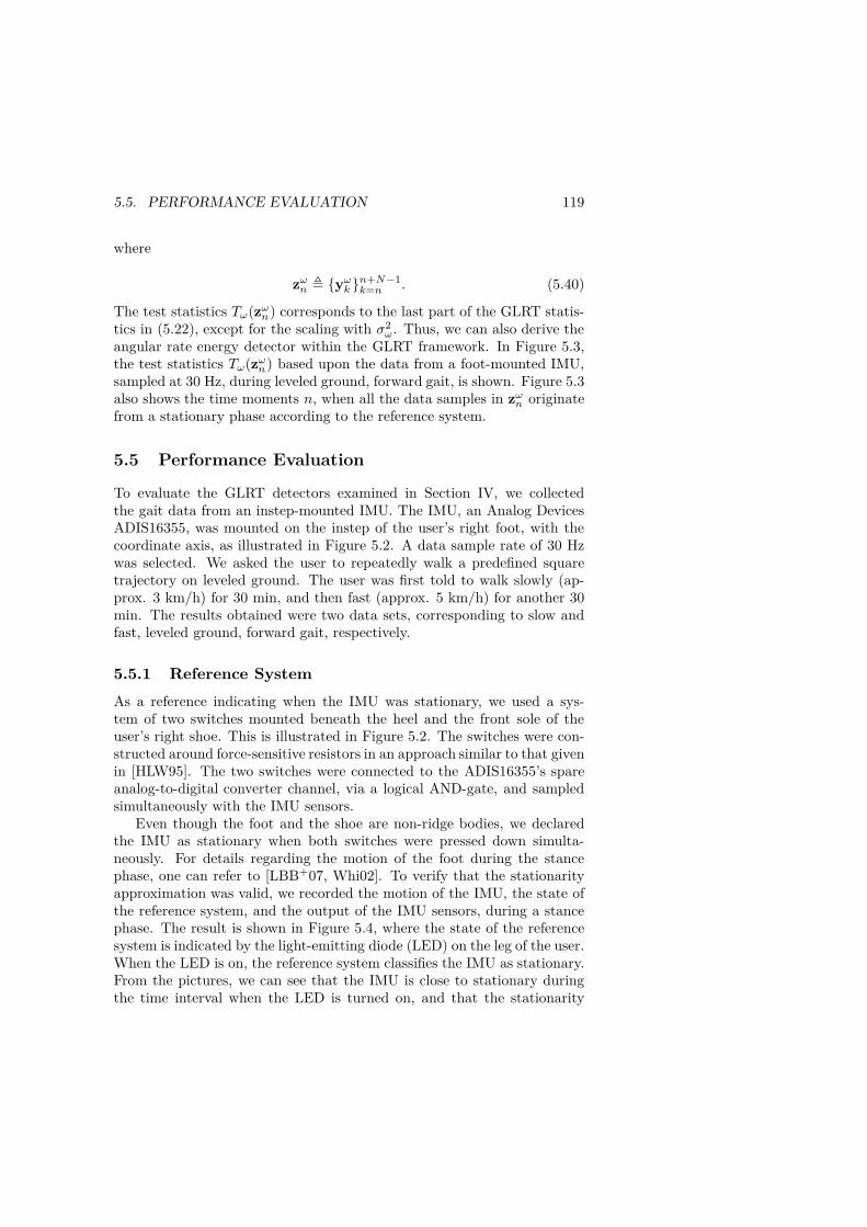
5.5. PERFORMANCE EVALUATION 119
where
zωn , yωk n+N−1k=n . (5.40)
The test statistics Tω(zωn) corresponds to the last part of the GLRT statis-tics in (5.22), except for the scaling with σ2
ω. Thus, we can also derive theangular rate energy detector within the GLRT framework. In Figure 5.3,the test statistics Tω(zωn) based upon the data from a foot-mounted IMU,sampled at 30 Hz, during leveled ground, forward gait, is shown. Figure 5.3also shows the time moments n, when all the data samples in zωn originatefrom a stationary phase according to the reference system.
5.5 Performance Evaluation
To evaluate the GLRT detectors examined in Section IV, we collectedthe gait data from an instep-mounted IMU. The IMU, an Analog DevicesADIS16355, was mounted on the instep of the user’s right foot, with thecoordinate axis, as illustrated in Figure 5.2. A data sample rate of 30 Hzwas selected. We asked the user to repeatedly walk a predefined squaretrajectory on leveled ground. The user was first told to walk slowly (ap-prox. 3 km/h) for 30 min, and then fast (approx. 5 km/h) for another 30min. The results obtained were two data sets, corresponding to slow andfast, leveled ground, forward gait, respectively.
5.5.1 Reference System
As a reference indicating when the IMU was stationary, we used a sys-tem of two switches mounted beneath the heel and the front sole of theuser’s right shoe. This is illustrated in Figure 5.2. The switches were con-structed around force-sensitive resistors in an approach similar to that givenin [HLW95]. The two switches were connected to the ADIS16355’s spareanalog-to-digital converter channel, via a logical AND-gate, and sampledsimultaneously with the IMU sensors.
Even though the foot and the shoe are non-ridge bodies, we declaredthe IMU as stationary when both switches were pressed down simulta-neously. For details regarding the motion of the foot during the stancephase, one can refer to [LBB+07, Whi02]. To verify that the stationarityapproximation was valid, we recorded the motion of the IMU, the state ofthe reference system, and the output of the IMU sensors, during a stancephase. The result is shown in Figure 5.4, where the state of the referencesystem is indicated by the light-emitting diode (LED) on the leg of the user.When the LED is on, the reference system classifies the IMU as stationary.From the pictures, we can see that the IMU is close to stationary duringthe time interval when the LED is turned on, and that the stationarity

120 CHAPTER 5. ZERO-VELOCITY DETECTION
approximation is valid3. However, one should note that the behavior ofthe reference system depends upon several factors such as the precise placeof the switches beneath the user’s shoe, the pronation or supination of theuser’s foot, etc. Thus, the results presented next should be regarded as anindication of the achievable performance, rather than an absolute measure.
5.5.2 Detector Statistics
Having collected the data, we calculated the detection and false-alarm prob-abilities for the detectors using a data window size N = 5 (i.e., approx. 167ms). The calculated probabilities for slow and fast gait are shown in Fig-ures 5.5 and 5.6, respectively. From the figures, we can see that:
• The angular rate energy detector and the new GLRT detector havethe highest performance, and behave basically in the same manner,indicating that the gyroscope signal holds the most reliable informa-tion for stationarity detection.
• There is a significant difference in the performance of the detectorsfor slow and fast gait, respectively.
At first glance it may seem that the performance of the detectors isfar from sufficient for any zero-velocity constrained navigation application.However, the PD versus PFA figures are partly misleading for our applica-tion. For a zero-velocity-constrained INS, it is better to have short periodsof zero-velocity updates on a regular basis at a low PFA level, than applyinglonger periods of zero-velocity updates at a higher PFA level. Thus, if thedetector’s threshold is adjusted to a lower PFA level, but the detector isstill capable of detecting that the IMU is stationary at least once for mostgait cycles, then the periods of free inertial navigation will be sufficientlyshort to avoid large error drifts.
A better measure of the performance of zero-velocity detectors is theprobability of detecting at least once that the IMU is stationary in the”IMU stationary” part of the gait cycle. We therefore introduced PSD, thatdenotes the probability that the detector decides on H1 at least once in the”IMU stationary” part of the gait cycle. By recalculating the statisticsof the detector in terms of PSD, using the data sets previously employed,we obtained the results for slow and fast forward gait, which are shown inFigures 5.7 and 5.8, respectively. From the figures, we can conclude that:
3The IMU will never be truly stationary during the stance phase. However, the smallmotions during the times of zero-velocity updates may be considered as the measurementnoise, and the covariance matrix associated with the pseudo observations should be setto reflect the size of these motions.

5.5. PERFORMANCE EVALUATION 121
0 0.05 0.1 0.15 0.2 0.25−2
0
2
0 0.05 0.1 0.15 0.2 0.25
−200
0
200
0.25 0.3 0.35 0.4 0.45 0.5−1
0
1
0.25 0.3 0.35 0.4 0.45 0.5−100
0
100
Accelerometer signals
Accelerometer signals
Gyroscope signals
Gyroscope signals
[g]
[g]
[/s]
[/s]
Time [s]
Time [s]Foot position
Foot position
Figure 5.4: The stance phase as a function of time together with the outputfrom the accelerometers and gyroscopes. When the LED is on (white dot inthe pictures), the reference system classifies the IMU as stationary. Legend:−· x-axis, −− y-axis, —- z-axis.

122 CHAPTER 5. ZERO-VELOCITY DETECTION
0 0.001 0.002 0.003 0.004 0.005 0.006 0.007 0.008 0.009 0.010
0.1
0.2
0.3
0.4
0.5
0.6
0.7
0.8
0.9
1
PFA
PD
PD versus PFA for slow, leveled ground, forward gait
T (zn)
T ′v(zan)
Tm(zan)
Tω(zωn)
Figure 5.5: PD versus PFA for the GLRT algorithms based upon data fromslow, leveled ground, forward gait. The detectors used a data window sizeof N = 5.
0 0.001 0.002 0.003 0.004 0.005 0.006 0.007 0.008 0.009 0.010
0.1
0.2
0.3
0.4
0.5
0.6
0.7
0.8
0.9
1
PFA
PD
PD versus PFA for fast, leveled ground, forward gait
T (zn)
T ′v(zan)
Tm(zan)
Tω(zωn)
Figure 5.6: PD versus PFA for the GLRT algorithms based upon data fromfast, leveled ground, forward gait. The detectors used a data window sizeof N = 5.
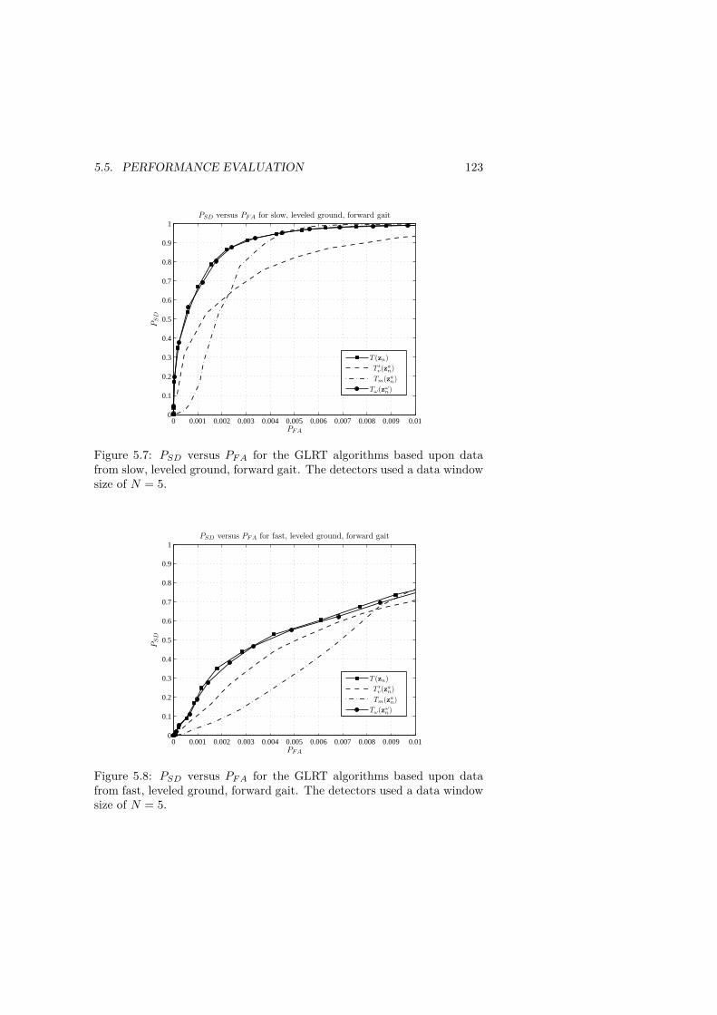
5.5. PERFORMANCE EVALUATION 123
0 0.001 0.002 0.003 0.004 0.005 0.006 0.007 0.008 0.009 0.010
0.1
0.2
0.3
0.4
0.5
0.6
0.7
0.8
0.9
1
PFA
PSD
PSD versus PFA for slow, leveled ground, forward gait
T (zn)
T ′v(zan)
Tm(zan)
Tω(zωn)
Figure 5.7: PSD versus PFA for the GLRT algorithms based upon datafrom slow, leveled ground, forward gait. The detectors used a data windowsize of N = 5.
0 0.001 0.002 0.003 0.004 0.005 0.006 0.007 0.008 0.009 0.010
0.1
0.2
0.3
0.4
0.5
0.6
0.7
0.8
0.9
1
PFA
PSD
PSD versus PFA for fast, leveled ground, forward gait
T (zn)
T ′v(zan)
Tm(zan)
Tω(zωn)
Figure 5.8: PSD versus PFA for the GLRT algorithms based upon datafrom fast, leveled ground, forward gait. The detectors used a data windowsize of N = 5.
124 CHAPTER 5. ZERO-VELOCITY DETECTION
• For slow gait at low PFA values, the angular rate energy detector andthe new GLRT detector still have the highest performance, whereasfor high PFA values, the magnitude detector has the best perfor-mance.
• For fast gait, the new GLRT detector is marginally better than theangular rate energy detector outperforming the other detector for allPFA values.
5.6 Conclusions
We have investigated the problem of detecting the time epochs when zero-velocity updates can be applied in a foot-mounted pedestrian navigationsystem. We have looked at three commonly used detectors, in the litera-ture: the acceleration moving variance detector, the acceleration magnitudedetector, and the angular rate energy detector. We have shown that alldetectors can be derived within the same GLRT framework - given the dif-ferent prior knowledge about the sensor signals. Further, by combining allprior knowledge, we derived a new GLRT detector. We subsequently eval-uated the performance of the detectors using slow (approx. 3 km/h) andfast (approx. 5 km/h), leveled ground, forward gait data. As a referencesystem, indicating when the IMU was stationary, we used force-sensitiveresistors mounted beneath the foot of the user. The test results were pre-sented in terms of the detection versus false-alarm probability. Moreover,we calculated the probability of detecting at least once that the IMU isstationary in ”IMU stationary” part of the gait cycle. This probability,being a function of the false-alarm probability, is often a better figure ofmerit for zero-velocity detectors used in constrained INSs.
The results show that the new GLRT detector performs similar to theangular rate energy detector [FZGB09, OB07], which outperforms both theacceleration moving variance detector [VBdV+96, GLC06, KLC08, GL08]and acceleration magnitude detector [GLC06, GL08, KR08]. This indi-cates that the gyroscope signals hold the most reliable information forzero-velocity detection under the experimental condition stated. Further,the results show that the performance varies a lot between slow and fastgait, where for the latter, the proper work of the detectors is questionable.
In the literature, there are rarely any discussions about the performanceof accelerometer-based detectors versus the ones based on gyroscope sig-nals. The majority of the works consider the former class of methods. Areason for this can be the fact that inexpensive off-the-shelf (COTS) ac-celerometers were available on the market some years before the gyroscopes.For instance, Analog Devices launched their first COTS accelerometer inthe beginning of the nineties, but their first gyroscope did not hit themarket until a decade later. Nowadays, six degrees-of-freedom IMUs are

5.6. CONCLUSIONS 125
readily available which opens up for detectors utilizing all six dimensions.We have shown that under the given assumptions the gyroscope-based de-tection clearly outperforms the accelerometer-based ones, and that thereis no significant improvement of the detector using the both accelerome-ter and gyroscope data, over the one only employing the signals from thegyroscopes.


Chapter 6
Calibration of a MEMS Inertial
Measurement Unit
6.1 Introduction
The development in micro-electro-mechanical system (MEMS) technologyhas made it possible to fabricate cheap single chip accelerometer and gy-roscope sensors, which have been adopted into many applications wheretraditionally inertial sensors have been too costly. For example the MEMSsensors have made it possible to construct low-cost global navigation satel-lite system (GNSS) aided inertial navigation systems (INS) for monitoringvehicle behavior [SSH06]. The obtained accuracy and convergence time ofa GNSS aided INS is highly dependent on the quality of the inertial mea-surement unit (IMU) sensors output [ESNN04], and therefore a calibrationof the IMU is critical for the over all system performance.
Traditionally the calibration of an IMU has been done using a mechan-ical platform, turning the IMU into different precisely controlled orienta-tions and at known rotational velocities [Rog03, Cha97, HTW89]. At eachorientation and during the rotations the output of the accelerometers andgyroscopes are observed and compared with the precalculated force and ro-tational velocity, respectively. However, the cost of a mechanical platformcan many times exceed the cost of developing and constructing a MEMSsensor based IMU. Therefore, in [KG04] a calibration procedure using aoptical tracking system is studied. In [Cha97, WWG02] calibration pro-cedures for the accelerometer cluster, where the requirements of a precisecontrol of the IMU’s orientation is relaxed are proposed. These calibra-tion methods utilize the fact that given a set of ideal sensors the norm ofthe measured output of the accelerometer and gyroscope cluster should beequal to the magnitude of the applied force and rotational velocity, respec-tively. However there are one major disadvantage with such a method; not
127
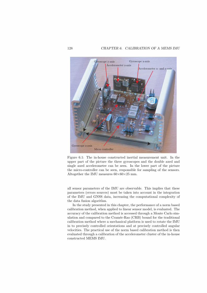
128 CHAPTER 6. CALIBRATION OF A MEMS IMU
Accelerometer x- and y-axisAccelerometer z-axis
Micro controller
Gyroscope x-axisGyroscope y-axis
Gyroscope z-axis
60m
m
60 mm
Figure 6.1: The in-house constructed inertial measurement unit. In theupper part of the picture the three gyroscopes and the double axed andsingle axed accelerometer can be seen. In the lower part of the picturethe micro-controller can be seen, responsible for sampling of the sensors.Altogether the IMU measures 60×60×25 mm.
all sensor parameters of the IMU are observable. This implies that theseparameters (errors sources) most be taken into account in the integrationof the IMU and GNSS data, increasing the computational complexity ofthe data fusion algorithm.
In the study presented in this chapter, the performance of a norm basedcalibration method, when applied to linear sensor model, is evaluated. Theaccuracy of the calibration method is accessed through a Monte Carlo sim-ulation and compared to the Cramér-Rao (CRB) bound for the traditionalcalibration method where a mechanical platform is used to rotate the IMUin to precisely controlled orientations and at precisely controlled angularvelocities. The practical use of the norm based calibration method is thenevaluated through a calibration of the accelerometer cluster of the in-houseconstructed MEMS IMU.
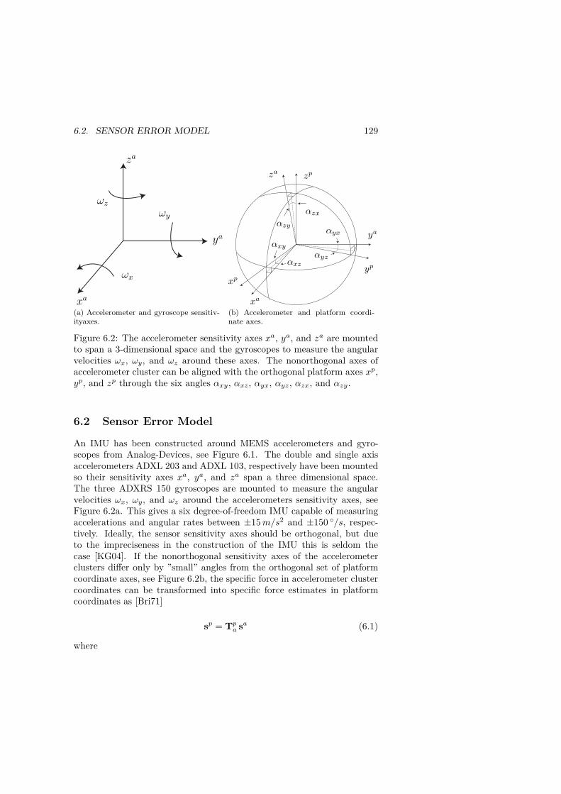
6.2. SENSOR ERROR MODEL 129
xa
ya
za
ωx
ωy
ωz
(a) Accelerometer and gyroscope sensitiv-ityaxes.
xpyp
zp
xa
ya
za
αxy
αxzαyz
αyx
αzxαzy
(b) Accelerometer and platform coordi-nate axes.
Figure 6.2: The accelerometer sensitivity axes xa, ya, and za are mountedto span a 3-dimensional space and the gyroscopes to measure the angularvelocities ωx, ωy, and ωz around these axes. The nonorthogonal axes ofaccelerometer cluster can be aligned with the orthogonal platform axes xp,yp, and zp through the six angles αxy, αxz, αyx, αyz, αzx, and αzy.
6.2 Sensor Error Model
An IMU has been constructed around MEMS accelerometers and gyro-scopes from Analog-Devices, see Figure 6.1. The double and single axisaccelerometers ADXL 203 and ADXL 103, respectively have been mountedso their sensitivity axes xa, ya, and za span a three dimensional space.The three ADXRS 150 gyroscopes are mounted to measure the angularvelocities ωx, ωy, and ωz around the accelerometers sensitivity axes, seeFigure 6.2a. This gives a six degree-of-freedom IMU capable of measuringaccelerations and angular rates between ±15m/s2 and ±150 /s, respec-tively. Ideally, the sensor sensitivity axes should be orthogonal, but dueto the impreciseness in the construction of the IMU this is seldom thecase [KG04]. If the nonorthogonal sensitivity axes of the accelerometerclusters differ only by ”small” angles from the orthogonal set of platformcoordinate axes, see Figure 6.2b, the specific force in accelerometer clustercoordinates can be transformed into specific force estimates in platformcoordinates as [Bri71]
sp = Tpa sa (6.1)
where
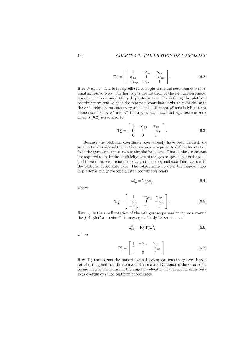
130 CHAPTER 6. CALIBRATION OF A MEMS IMU
Tpa =
1 −αyz αzyαxz 1 −αzx−αxy αyx 1
. (6.2)
Here sp and sa denote the specific force in platform and accelerometer coor-dinates, respectively. Further, αij is the rotation of the i-th accelerometersensitivity axis around the j-th platform axis. By defining the platformcoordinate system so that the platform coordinate axis xp coincides withthe xa accelerometer sensitivity axis, and so that the yp axis is lying in theplane spanned by xa and ya the angles αxz, αxy, and αyx become zero.That is (6.2) is reduced to
Tpa =
1 −αyz αzy0 1 −αzx0 0 1
. (6.3)
Because the platform coordinate axes already have been defined, sixsmall rotations around the platforms axes are required to define the rotationfrom the gyroscope input axes to the platform axes. That is, three rotationsare required to make the sensitivity axes of the gyroscope cluster orthogonaland three rotations are needed to align the orthogonal coordinate axes withthe platform coordinate axes. The relationship between the angular ratesin platform and gyroscope cluster coordinates reads
ωpip = Tpgωgig (6.4)
where
Tpg =
1 −γyz γzyγxz 1 −γzx−γxy γyx 1
. (6.5)
Here γij is the small rotation of the i-th gyroscope sensitivity axis aroundthe j-th platform axis. This may equivalently be written as
ωpip = RpoTogωgig (6.6)
where
Tog =
1 −γyz γzy0 1 −γzx0 0 1
. (6.7)
Here Tog transforms the nonorthogonal gyroscope sensitivity axes into aset of orthogonal coordinate axes. The matrix Rpo denotes the directionalcosine matrix transforming the angular velocities in orthogonal sensitivityaxes coordinates into platform coordinates.

6.2. SENSOR ERROR MODEL 131
V (f) [V olt]
f [g]
bias
∆V
∆f
non− linearity
Kai = ∆V∆f
Figure 6.3: The relationship between the output voltage of the accelerom-eter (gyroscope) and the measured force (angular rate) is modelled as alinear function, describing the scaling and bias of the sensors.
The MEMS sensors output a voltage proportional to the physical quan-tities sensed by the sensors, acceleration and angular rates, respectively.The typical relationship between the output voltage and the physical quan-tity acting along the sensor sensitivity axes is given by the manufacturesdata sheet, but the true scaling varies between different specimens and withthe input signal (due to inherent nonlinearities of the sensors). Moreover,there is often a small bias in the sensor output signal, that is even thoughthere is no force acting onto the sensor, the sensor produces a non-zerooutput, see Figure 6.3. For the MEMS sensors used in our applicationthe nonlinearities are in the order 0.1% of a best fit to a straight line andtherefore neglected. Next, introduce the accelerometer scale factor matrixKa and bias vector ba defined as
Ka = diag(kxa , kya , kza) (6.8)
and
ba = [ bxa bya bza ]T , (6.9)

132 CHAPTER 6. CALIBRATION OF A MEMS IMU
where kia and bia are the unknown scaling and bias of the i-th accelerometeroutput, respectively. Further (·)T denotes the transpose operation anddiag(·) the diagonal matrix with the elements given within the parentheses.The measured output of the accelerometer cluster may then be modelledas [Cha97]
sa = Ka (Tpa)−1 sp + ba + va (6.10)
where sa = (Tpa)−1sp from (6.1) was employed. In (6.10), va is a noise
term reflecting the measurement noise from the sensors. Applying the samemodel to the MEMS gyroscopes, the output from the gyroscope-cluster maybe written as
ωgig = Kg ωgig + bg + vg
= Kg (Tog)−1 Rop ω
pip + bg + vg
(6.11)
where Kg and bg are the scale factor matrix and bias vector of the gyroscope-cluster, respectively. Further ωpip is the true rotational rate of the IMUplatform with respect to the inertial frame of reference and vg is the gy-roscope measurement noise. In the second equality in (6.11) the notationRop = (Rpo)
−1 has been used to denote the directional cosine matrix, rotat-ing a vector from platform coordinates to the coordinate system associatedwith the orthogonal gyroscope sensitivity axes. Worth noting is that themisalignment matrices Tpa and Tog are constant matrices only dependent onthe physical mounting of the components. Ka,Kg,ba and bg may be splitinto a static part, a temperature varying and a random drift part [GWA07].The temperature varying and random drift part must be taken into accountby the integration algorithm, fusing the GNSS and IMU data. Thereforethe prime goal of the calibration is to estimate Tpa and Tog and the staticparts of the scale factors and biases.
Both the accelerometer and gyroscope cluster model fit into the moregeneral signal model described by Figure 6.4. Here the input uk corre-sponds to the specific force sp at time k in the accelerometer cluster modelor the angular velocity ωoip = Rop ω
pip in the gyroscope cluster model.
6.3 Calibration Algorithm
Traditionally, a mechanical platform rotating the IMU into different pre-cisely controlled orientations and angular rates has been used to calibrateIMU’s. Then, observing the output yk and the precalculated specific forceor angular velocity uk acting upon the IMU for 12 or more different orienta-tions and rotation sequences, respectively it is straightforward to estimatethe misalignment, scaling and bias [Rog03, Cha97, HTW89]. Note, that

6.3. CALIBRATION ALGORITHM 133replacemen
Soughtphysicalquantity
uk Sensoroutput
yk
vk
KT−1
b
Figure 6.4: Sensor model including misalignments T−1, scale factors K,biases b, and measurement noise vk.
there are 9 and 12 unknowns in the signal models, respectively - threescale factors, three biases, three orthogonal rotations and in addition forthe gyroscope cluster the three rotations aligning the orthogonal gyroscopecoordinate axes with the platform axes. The cost of a mechanical platformoften exceeds the cost of developing and constructing a MEMS sensor basedIMU. Therefore a calibration procedure is desirable where the requirementsof a precisely controlled orientation of the IMU can be relaxed.
Based upon the signal model in Figure 6.4 a natural estimator for theinput uk based on the sensor output yk is
uk = h(yk, θ) = T K−1(yk − b) (6.12)
where the sought parameters are collected in the parameter vector
θ =[kx ky kz αyz αzy αzx bx by bz σ
2]T. (6.13)
In order to have a more unified notation throughout the chapter the noisevariance has been included in the parameter vector in (6.13). However,the proposed estimator does not depend on the noise variance and it cantherefore be omitted in equations (6.12)-(6.19).
Ideally, independent of the orientation of the IMU, the magnitude ofthe measured gravity force and angular velocity should be equal to themagnitude of the apparent gravity force and applied angular velocity, re-spectively. Therefore, the squared error between the squared magnitude ofthe input uk and the squared magnitude of the output from the compen-sated IMU output may serve as a cost function when calibrating the IMU.That is
θ = argminθL(θ) (6.14)
where
L(θ) =K−1∑
k=0
(‖uk‖2 − ‖h(yk, θ)‖2)2. (6.15)
Here, K = M N , where M is the number of orientations or rotations thatthe platform is exposed too and N the number of samples taken during

134 CHAPTER 6. CALIBRATION OF A MEMS IMU
each rotation or at each orientation. Still, since there are nine unknownsthe platform must be exposed to nine or more orientations and rotations,respectively. However, the demand of a precise control of the orientationis relaxed. Worth noting when calibrating the gyroscopes is that
‖uk‖2 = ‖ωoip‖2 = ‖Rop ωpip‖2 = ‖ωpip‖2 (6.16)
where in the last equality the fact that the directional cosine matrix Ropis an orthonormal matrix, i.e., (Rop)
T (Rop) = I3, has been used. Here I3
is the identity matrix of size 3. Therefore the three Euler angles relatingthe orthogonal coordinate axes of the gyroscope cluster and the platformcoordinates are unobservable when the magnitudes are used to calibratethe IMU.
At each orientation of the IMU, the specific force acting along the ac-celerometers sensitivity axes are constant, i.e., the input uk is constantduring the N samples. This also holds for the gyroscope cluster model, ifassuming that during each rotation of the IMU the rotation velocity is keptconstant. The cost function may then be simplified as
L(θ) =M−1∑
m=0
(‖um‖2 − ‖h(ym, θ)‖2)2 (6.17)
where um and ym are the input and sample mean at the m-th orientationand rotation, respectively. This reduced cost function may be minimizedusing for example Newton’s method, that is [BV04]
θk+1 = θk +
[d2L(θ)
dθ dθT
]−1dL(θ)
dθ
∣∣∣∣θ=θk
(6.18)
θ0 ∈ domain of attraction.The cost function in (6.15) has several local optima and to ensure thatthe recursion (6.18) converges to the true parameters the search for theminima must be initialized with a θ in the domain of attraction of the globalminima. According to the data sheet of the accelerometers the scale factorsdiffer less then 6% from there nominal values (unit gain) and the biases aresmaller then ±1m/s2. Further the misalignments can be assumed small.Therefore an appropriate initial value for the parameter vector may be
θ0 =[
1 1 1 0 0 0 0 0 0 σ2]T. (6.19)
6.4 Cramér-Rao Bound
When evaluating the performance of an estimator it is often of interestto compare the estimation error of the estimator with that of an opti-
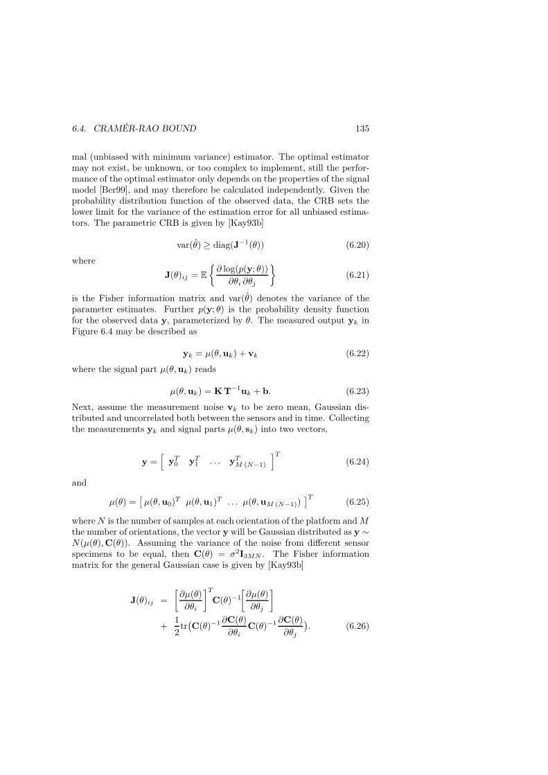
6.4. CRAMÉR-RAO BOUND 135
mal (unbiased with minimum variance) estimator. The optimal estimatormay not exist, be unknown, or too complex to implement, still the perfor-mance of the optimal estimator only depends on the properties of the signalmodel [Ber99], and may therefore be calculated independently. Given theprobability distribution function of the observed data, the CRB sets thelower limit for the variance of the estimation error for all unbiased estima-tors. The parametric CRB is given by [Kay93b]
var(θ) ≥ diag(J−1(θ)) (6.20)
where
J(θ)ij = E
∂ log(p(y; θ))
∂θi ∂θj
(6.21)
is the Fisher information matrix and var(θ) denotes the variance of theparameter estimates. Further p(y; θ) is the probability density functionfor the observed data y, parameterized by θ. The measured output yk inFigure 6.4 may be described as
yk = µ(θ,uk) + vk (6.22)
where the signal part µ(θ,uk) reads
µ(θ,uk) = K T−1uk + b. (6.23)
Next, assume the measurement noise vk to be zero mean, Gaussian dis-tributed and uncorrelated both between the sensors and in time. Collectingthe measurements yk and signal parts µ(θ, sk) into two vectors,
y =[
yT0 yT1 . . . yTM (N−1)
]T(6.24)
and
µ(θ) =[µ(θ,u0)T µ(θ,u1)T . . . µ(θ,uM (N−1))
]T(6.25)
whereN is the number of samples at each orientation of the platform andMthe number of orientations, the vector y will be Gaussian distributed as y ∼N(µ(θ),C(θ)). Assuming the variance of the noise from different sensorspecimens to be equal, then C(θ) = σ2I3MN . The Fisher informationmatrix for the general Gaussian case is given by [Kay93b]
J(θ)ij =
[∂µ(θ)
∂θi
]TC(θ)−1
[∂µ(θ)
∂θj
]
+1
2tr(C(θ)−1 ∂C(θ)
∂θiC(θ)−1 ∂C(θ)
∂θj
). (6.26)
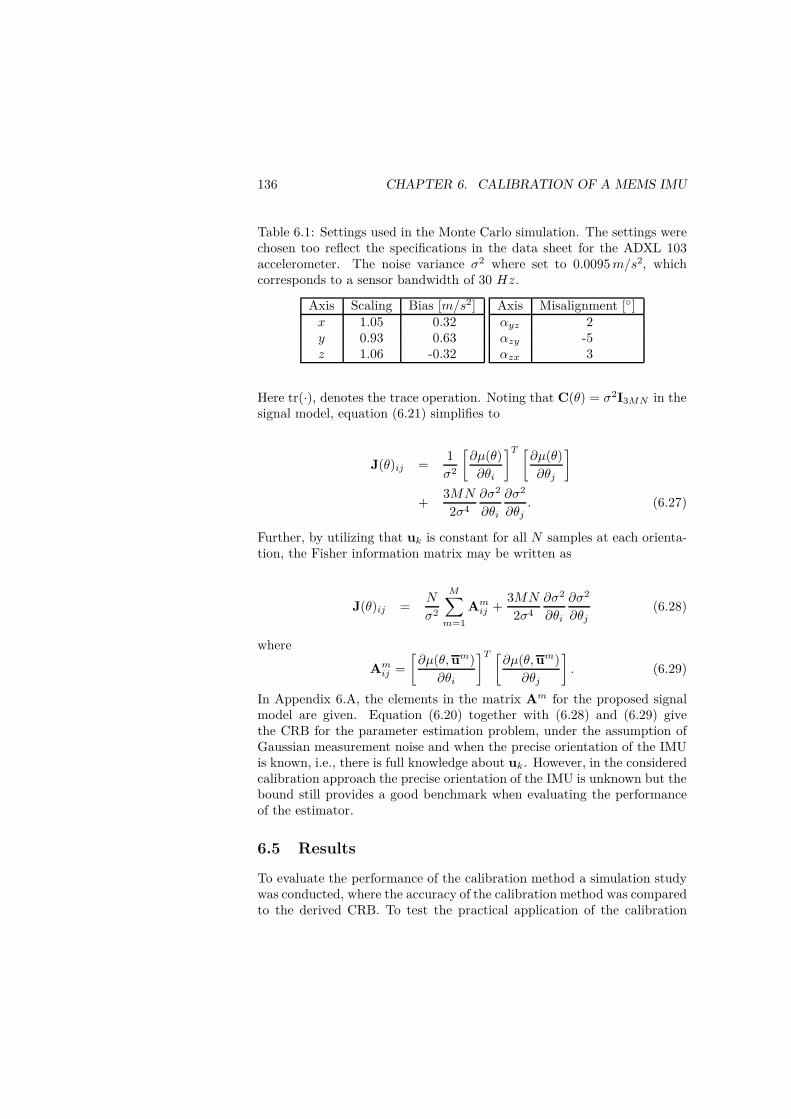
136 CHAPTER 6. CALIBRATION OF A MEMS IMU
Table 6.1: Settings used in the Monte Carlo simulation. The settings werechosen too reflect the specifications in the data sheet for the ADXL 103accelerometer. The noise variance σ2 where set to 0.0095m/s2, whichcorresponds to a sensor bandwidth of 30 Hz.
Axis Scaling Bias [m/s2]x 1.05 0.32y 0.93 0.63z 1.06 -0.32
Axis Misalignment []αyz 2αzy -5αzx 3
Here tr(·), denotes the trace operation. Noting that C(θ) = σ2I3MN in thesignal model, equation (6.21) simplifies to
J(θ)ij =1
σ2
[∂µ(θ)
∂θi
]T [∂µ(θ)
∂θj
]
+3MN
2σ4
∂σ2
∂θi
∂σ2
∂θj. (6.27)
Further, by utilizing that uk is constant for all N samples at each orienta-tion, the Fisher information matrix may be written as
J(θ)ij =N
σ2
M∑
m=1
Amij +3MN
2σ4
∂σ2
∂θi
∂σ2
∂θj(6.28)
where
Amij =
[∂µ(θ,um)
∂θi
]T [∂µ(θ,um)
∂θj
]. (6.29)
In Appendix 6.A, the elements in the matrix Am for the proposed signalmodel are given. Equation (6.20) together with (6.28) and (6.29) givethe CRB for the parameter estimation problem, under the assumption ofGaussian measurement noise and when the precise orientation of the IMUis known, i.e., there is full knowledge about uk. However, in the consideredcalibration approach the precise orientation of the IMU is unknown but thebound still provides a good benchmark when evaluating the performanceof the estimator.
6.5 Results
To evaluate the performance of the calibration method a simulation studywas conducted, where the accuracy of the calibration method was comparedto the derived CRB. To test the practical application of the calibration

6.5. RESULTS 137
Table 6.2: IMU results. The average estimate of the accelerometer clus-ter parameters, calculated from 20 calibration of the in-house constructedIMU. At each calibration the platform was rotated into 18 different orien-tation and at each orientation the sensors were sampled 100 times.
Axis Scaling Bias [m/s2]x 0.998 -0.435y 0.996 0.254z 1.008 0.099
Axis Misalignment []αyz 0.026αzy -0.695αzx 1.808
0.2 0.4 0.6 0.8 1 1.2 1.4 1.6 1.8 265
70
75
80
85
90Scale factors
10log 1
0(1/M
SE
)
10 log10(N)
kxkykzCRB
Figure 6.5: Empirical MSE of the scale factor estimates as a function ofthe number of samples.
method the accelerometer cluster of the in-house constructed IMU wascalibrated.
6.5.1 Performance Evaluation
The proposed calibration approach has been evaluated by Monte Carlosimulations. In the simulation, the estimation of the accelerometer clus-ter parameters were studied when the IMU was rotated into 18 differentorientations, as proposed in [Cha97]. However, a uniformly distributed er-ror between [−5, 5] was added to the proposed orientations to reflect the

138 CHAPTER 6. CALIBRATION OF A MEMS IMU
0.2 0.4 0.6 0.8 1 1.2 1.4 1.6 1.8 260
65
70
75
80
85
90Misalignment
10log 1
0(1/M
SE
)
10 log10(N)
αyzαzyαzxCRBx
CRBy
CRBz
Figure 6.6: Empirical MSE of the misalignment angle estimates as a func-tion of the number of samples.
relaxed demands of a precise orientation. In Figure 6.5, 6.6, and 6.7 theempirical mean square error for the scale-factors, misalignment angles, andbiases estimates are shown, calculated from 1000 simulated calibrationsusing the proposed calibration approach. The solid line is the CRB forthe calibration, when the the precise orientation of the IMU is known. InTable 6.1, the settings used in the simulation are summarized.
As can be seen from Figure 6.5, 6.6, and 6.7 the performance of theproposed calibration procedure is approximately 2, 8, and 5 decibel bellowthe CRB for the scale factors, misalignments, and biases, respectively. Stillthe root mean square error, when 100 samples are taken at each orientation,of the estimated parameters are less than 10−2 of the magnitude of theparameters, and may therefore normally be considered acceptable for low-cost applications.
6.5.2 IMU Calibration
The accelerometer cluster of the in-house constructed IMU has been cali-brated using the proposed method. The IMU was by hand placed into 18different positions, the six sides and the twelve edges of the IMU. At eachorientation 100 samples were taken. In Table 6.2, the average parameter

6.6. CONCLUSIONS 139
0.2 0.4 0.6 0.8 1 1.2 1.4 1.6 1.8 250
55
60
65
70
75Bias
10log 1
0(1/M
SE
)
10 log10(N)
bxbybzCRB
Figure 6.7: Empirical MSE of the bias estimates as a function of the numberof samples.
estimate out of 20 calibrations are shown. All the obtained estimates are inthe expected region for the used sensors, that is the scale factor diverge lessthan 6% from the unit gain and the biases are less then 1m/s2. The esti-mated misalignment angle αyz, as can be seen in Figure 6.2b correspondsto the misalignment between the x- and y-axis in the IMU, which should beclose to zero. This is due to the fact that the x- and y-accelerometers aremounted into the same MEMS sensor case. The remaining two misalign-ments angles correspond to the misalignment between the x- and z-axisrespectively y- and z-axis, which due to the impreciseness when the IMUwas constructed, should be much larger. See Figure 6.1.
6.6 Conclusions
A MEMS sensor based inertial measurement unit has been constructed in-house, intended to be used in a low-cost GNSS aided inertial navigationsystems. In order to improve the performance of the GNSS aided INS,which is highly dependent on the accuracy of the IMU, an approach forcalibrating the IMU, requiring no mechanical platform for the accelerom-eter calibration and only a simple rotating table for the gyroscope cali-
140 CHAPTER 6. CALIBRATION OF A MEMS IMU
bration has been studied. The performance of the calibration algorithmis compared with the CRB for the traditional calibration method, wherea mechanical platform is used to rotate the IMU into different preciselycontrolled orientations. Simulation results shows that the mean square er-ror of the parameter estimates of the senor model increases with up to 8decibel, when utilizing the proposed method. Further, not all parametersin the gyroscope sensor model are observable with the proposed calibra-tion approach. This can increasing the computational complexity of theGNSS aided INS, which may have to estimate several additional systemparameters. Still the proposed method can be considered acceptable anduseful for many low-cost applications where the cost of constructing a me-chanical platform many times can exceed the cost of developing the inertialmeasurement unit.

6.A. FIM ELEMENTS 141
6.A FIM Elements
The nonzero elements in Am are
Am1,1 = (umx + αzyumy + (αyzαzx − αzy)umz )2
Am1,4 = (umx + αzyumy + (αyzαzx − αzy)umz )(kxu
my + αzxkxu
mz )
Am1,5 = (umx + αzyumy + (αyzαzx − αzy)umz )(−kxumz )
Am1,6 = (umx + αzyumy + (αyzαzx − αzy)umz )(αyzkxu
mz )
Am1,7 = (umx + αzyumy + (αyzαzx − αzy)umz )
Am2,2 = (umy + αzxumz )2
Am2,6 = (umy + αzxumz )kyu
mz
Am2,8 = (umy + αzxumz )
Am3,3 = (umz )2
Am3,9 = (umz )
Am4,4 = (kxumy + αzxkxu
mz )2
Am4,5 = (kxumy + αzxkxu
mz )(−kxumz )
Am4,6 = (kxumy + αzxkxu
mz )(αyzkxu
mz )
Am4,7 = (kxumy + αzxkxu
mz )
Am5,5 = (−kxumz )2
Am5,6 = (−kxumz )(αyzkxumz )
Am5,7 = (−kxumz )
Am6,6 = (αyzkxumz )2 + (kyu
mz )2
Am6,7 = (αyzkxumz )
Am6,8 = (kyumz )
Am7,7 = Am8,8 = Am9,9 = 1


Bibliography
[AAR03] S. Alban, D.M. Akos, and S.M. Rock. Performance analysisand architectures for INS-aided GPS tracking loops. In inProc. National Technical Meeting of the Institute of Navi-gation, ION-NTM 03., January 2003.
[All84] D. W. Allan. Clock characterization tutorial. In NRL Proc.of the 15th Ann. Precise Time and Time Interval (PTTI)Appl. and Planning Meeting, pages 459–475, April 1984.
[All87] D. W. Allan. Time and frequency (time-domain) characteri-zation, estimation, and prediction of precision clocks and os-cillators. IEEE Transactions on Ultrasonics, Ferroelectricsand Frequency Control, 34(6):647–654, November 1987.
[AP99] E. Abbott and D. Powell. Land-vehicle navigation usingGPS. Proceedings of the IEEE, 87(1):145–162, January1999.
[APM05] I. F. Akyildiz, D. Pompili, and T. Melodia. Underwateracoustic sensor networks: research challenges. Ad Hoc Net-works, 3(3):257–279, May 2005.
[ASK04] B. Azimi-Sadjadi and P. S. Krishnaprasad. A particlefiltering approach to change detection for nonlinear sys-tems. EURASIP, Journal on Applied Signal Processing,2004(15):2295–2305, 2004.
[ASK05] B. Azimi-Sadjadi and P. S. Krishnaprasad. Approximatenonlinear filtering with applications to navigation. Auto-matica, 41:945–956, 2005.
[ASNES06] P. Aggarwal, Z. Syed, X. Niu, and N. El-Sheimy. Cost-efficient testing and calibration of low cost MEMS sensorsfor integrated positioning, navigation and mapping systems.In Proc. XXIII FIG Congress, Munich, Germany, October2006.
143
144 BIBLIOGRAPHY
[ÅW84] K.J. Åström and B. Wittenmark. Computer Controlled Sys-tems: Theory and Design. Prentice Hall, 1984.
[BBS+08] S. Bamberg, A. Y. Benbasat, D. M. Scarborough, D. E.Krebs, and J. A. Paradiso. Gait analysis using a shoe-integrated wireless sensor system. IEEE Trans. InformationTechnology in Biomedicine, 12(4):413–423, July 2008.
[BD71] W. Bar and F. Dittrich. Useful formula for moment com-putation of normal random variables with non-zero means.IEEE Trans. on Automatic Control, AC-16:263–265, 1971.
[Ber99] N. Bergman. Recursive Bayesian Estimation, Navigationand Tracking Applications. PhD thesis, Dept. of ElectricalEngineering, Linköpings Univeristy, 1999.
[BF96] J. Borenstein and L. Feng. Measurement and correction ofsystematic odometry errors in mobile robots. IEEE Trans.Robotics and Automation, 12(6):869–880, December 1996.
[BIV85] I.Y. Bar-Itzhack and Y. Vitek. The enigma of false biasdetection in a strapdown system during transfer alignment.Journal of Guidance, Control and Dynamics, 8(2):175–180,March 1985.
[BJD07] P. Bonnifait, M. Jabbour, and G. Dherbomez. Real-timeimplementation of a GIS-based localization system for in-telligent vehicles. EURASIP Journal on Embedded Systems,2007:1–12, 2007.
[BK96] D. Bernstein and A. Kornhauser. An Introduction toMap Matching for personal navigation assistants. NewJersy TIDE Center http://www.njtide.org/reports/
mapmatchintro.pdf, 1996.
[BL04] A.K. Brown and Y. Lu. Preformance test results of an in-tegrated GPS/MEMS inertial navigation package. In Proc.ION GNSS Conf., pages 1251–1256, California, USA, March2004.
[BMR06] S. Bonnabel, P. Martin, and P. Rouchon. A non-linearsymmetry-preserving observer for velocity-aided inertialnavigation. In In Proc. of the 2006 American Control Con-ference, Minnesota, USA, June 2006.
[BO07] U.I. Bhatti and W.Y. Ochieng. Failure modes and modelsfor integrated GPS/INS systems. The Journal of Naviga-tion, 60:327–348, 2007.

145
[Bob05] B. Boberg. Robust navigation. Swedish Journal of MilitaryTechnology, (3):23–28, 2005.
[BOF07a] U.I. Bhatti, W.Y. Ochieng, and S. Feng. Integrity of an in-tegrated GPS/INS system in the presence of slowly growingerrors. Part I: A critical review. GPS Solutions, 11(3):173–181, 2007.
[BOF07b] U.I. Bhatti, W.Y. Ochieng, and S. Feng. Integrity of an in-tegrated GPS/INS system in the presence of slowly growingerrors. Part II: A analysis. GPS Solutions, 11(3):183–192,2007.
[BRB+06] J. Bryzek, S. Roundly, B. Bircumshaw, C. Chung,K. Castellino, J.R. Stetter, and M. Vestel. MarvelousMEMS. IEEE Circuits and Devices Magazine, 22(2):8–28,March–April 2006.
[Bre97] S. Bregni. Clock stability characterization and measurementin telecommunications. IEEE Trans. Instrumentation andMeasurement, 46(6):1284–1296, December 1997.
[BRG06] D.M. Bevly, J. Ryu, and J.C. Gerdes. Integrating INSsensors with GPS measurements for continuous estimationof vehicle sideslip, roll, and tire cornering stiffness. IEEETrans. on Intelligent Transportation Systems, 7(4):483–493,December 2006.
[Bri71] K.R. Britting. Inertial Navigation Systems Analysis. WileyInterscience, 1971.
[BS71] R.J. Brown and A.P. Sage. Estimation using stochasticfeedback with applications to integrated navigation sys-tems. IEEE Trans. on Aerospace and Electronic Systems,7(2):355–, March 1971.
[BS01] N. Barbour and G. Schmidt. Inertial sensor technologytrends. IEEE Sensors Journal, 1(4):332–339, December2001.
[BV04] S. Boyd and L. Vandenberghe. Convex Optimization. Cam-bridge, 2004.
[BW02] B. Boberg and S.L. Wirkander. Integrating GPS and INS:comparing the Kalman estimator and particle estimator. InIn Proc. of ICARCV 2002. 7-th International Conferenceon Control, Automation, Robotics and Vision, 2002., pages484–490, December 2002.

146 BIBLIOGRAPHY
[BW05] R. Babu and J. Wang. Analysis of INS derived dopplereffects on carrier tracking loop. Navigation, 58(3):493–507,September 2005.
[CATB04] R.K. Curey, M.E. Ash, L.O. Thielman, and C.H. Barker.Proposed IEEE inertial systems terminology standard andother inertial sensor standards. In Proc. Position Locationand Navigation Symposium, 2004. PLANS 2004, April 2004.
[CC06] S.Y. Cho and W.S. Choi. Robust positioning technique inlow-cost DR/GPS for land navigation. IEEE Trans. on Veh.Techn., 55(4):1132–1142, August 2006.
[CCF+06] E.T. Coelho, P. Carvalhal, M.J. Ferreira, L.F. Silva,H. Almeida, C. Santos, and J.A. Afonso. A bluetooth-based wireless distributed data acquisition and control sys-tem. In Proc. of IEEE International Conf. on Robotics andBiomimetics, 2006. ROBIO ’06., December 2006.
[CDDV07] F. Caron, M. Davy, E Duflos, and P. Vanheeghe. Particlefiltering for multisensor data fusion with switching observa-tion models: Application to land vehicle positioning. IEEETrans. on Signal Processing, 55(6):2703–2719, June 2007.
[CGES06] K.W. Chiang, C. Goodall, and N. El-Sheimy. Improving theattitude accuracy of INS/GPS integrated systems. EuropeanJournal of Navigation, 4(2):31–40, May 2006.
[CGP02] R.C. Carlson, J.C. Gerdes, and J.D. Powell. Practical po-sition and yaw rate estimation with GPS and differentialwheelspeeds. In Proc. AVEC 2002 6th Int. Symp. AdvancedVehicle Control, Hiroshima, Japan, September 2002.
[CGP04] R.C. Carlson, J.C. Gerdes, and J.D. Powell. Error sourceswhen land vehicle dead reckoning with differential wheel-speeds. Navigation, 51(1):13–27, 2004.
[CH08] K.W. Chiang and Y.W. Huanga. An intelligent navigatorfor seamless INS/GPS integrated land vehicle navigationapplications. Applied Soft Computing Journal, 8(1):722–733, January 2008.
[Cha97] Chatfield. Fundamentals of High Accuracy Inertial Naviga-tion. AIAA, 1997.
[CHNES04] K.W. Chiang, H. Hou, X. Niu, and N. El-Sheimy. Improvingthe positioning accuracy of DGPS/MEMS IMU integrated
147
systems utilizing cascade de-noising algorithm. In Proc.17thInternational Technical Meeting of the Satellite Division ofthe Institute of Navigation ION GNSS 2004, Long Beach,CA, USA, September 2004.
[CL04] R. Chen and X. Li. Virtual differential GPS based on SBASsignal. GPS Solutions, 8(4):238–244, September 2004.
[CLD94] J.H Chen, S.C Lee, and D.B. DeBra. Gyroscope freestrapdown inertial measurement unit by six linear ac-celerometers. Journal of Guidance, Control and Dynamics,17(2):286–290, 1994.
[CLYC05] W. Chen, Z. Li, M. Yu, and Y. Chen. Effects of sensorerrors on the performance of map matching. The Journalof Navigation, 58:273–282, 2005.
[CLYX06] X. Chaonong, Z. Lei, X. Yongjun, and L. Xiaowei. Timesynchronization simulator and its application. In Proc. of1ST IEEE Conf. on Industrial Electronics and Applications,2006.
[CSQ08a] Q. M. Chaudhari, E. Serpedin, and K. Qaraqe. Cramer-Raolower bound for the clock offset of silent nodes synchroniz-ing through a general sender-receiver protocol in wirelesssensornets. In Proc. EUSIPCO 2008, 16th European SignalProcessing Conference., 2008.
[CSQ08b] Q.M. Chaudhari, E. Serpedin, and K. Qaraqe. On maximumlikelihood estimation of clock offset and skew in networkswith exponential delays. IEEE Trans. on Signal Processing,56(4):1685–1697, 2008.
[CWCE06] V. Chandrasekhar, KG. S. Winston, Y. S. Choo, and H. V.Ee. Localization in underwater sensor networks: surveyand challenges. In Proc. of the 1st ACM Int. workshop onUnderwater networks, WUWNet ’06, 2006.
[Dau05] F. Daum. Nonlinear filters: Beyond the Kalman filter. IEEEAerospace and Electronic Systems Magazine, 20(8):57–69,August 2005.
[DB04] J. Du and M. Barth. Lane-level positioning for in-vehiclenavigation and automated vehicle location (AVL) systems.In Proc. ITSC 2004, 7th Int. IEEE Conf. on IntelligentTransportation Systems, pages 35–40, Washington, D.C,USA, October 2004.
148 BIBLIOGRAPHY
[DB06] J. Du and M. Barth. Bayesian probabilistic vehicle lanematching for link-level in-vehicle navigation. In Proc. ofIEEE Int. Veh. Symp., pages 522–526, Tokyo, Japan, June2006.
[DH03] F. Daum and J. Huang. Curse of dimensionality and particlefilters. In In Proc. of IEEE Aerospace Conference., March2003.
[DH04] H. Dai and R. Han. TSync: a lightweight bidirectionaltime synchronization service for wireless sensor networks.ACM SIGMOBILE Mobile Computing and Commun. Re-view, 8(1):125–139, January 2004.
[Dig07] .F Diggelen. GNSS Accuracy: Lies, Damm Lies, and Statis-tics. GPS World, (1):26–32, January 2007.
[Dix05] K. Dixon. Satellite positioning systems: Efficiencies, per-formance and trends. European Journal of Navigation,3(1):58–63, February 2005.
[DLES07] H Dongliang, H. Leung, and N. El-Sheimy. Expectationmaximization based GPS/INS integration for land-vehiclenavigation. IEEE Trans. on Aerospace and Electronic Sys-tems, 43(3):1168 – 1177, July 2007.
[DR98] C. Drane and C. Rizos. Positioning Systems in IntelligentTransportation Systems. Artech House, 1998.
[DSNDW01] G. Dissanayake, S. Sukkarieh, E. Nebot, and H. Durrant-Whyte. The aiding of a low-cost strapdown inertial mea-surement unit using vehicle model constraints for land ve-hicle applications. IEEE Trans. Robotics and Automation,17(5):731–747, October 2001.
[DWL+08] W. Ding, J. Wang, Y. Li, P. Mumford, and C. Rizos.Time synchronization error and calibration in integratedGPS/INS systems. ETRI Journal, 30(1):59–67, February2008.
[DWM+05] W.D. Ding, J.L. Wang, P. Mumford, Y. Li, and C. Rizos.Time synchronization design for integrated positioning andgeoreferencing systems. In Proc. SSC 2005 Spatial Intelli-gence, Innovation and Praxis: The national biennial Con-ference of the Spatial Sciences Institute, Melbourne, Aus-tralia, September 2005.

149
[EGE02] J. Elson, L. Girod, and D. Estrin. Fine-grained networktime synchronization using reference broadcasts. SIGOPSOper. Syst. Rev., 36:147–163, 2002.
[EHP00] M. Evans, N. Hastings, and B. Peacock. Statistical distri-butions. Wiley, 2000.
[EM99] P. Enge and P. Misra. Special issue on global positioningsystem. Proceedings of the IEEE, 87(1):3–15, January 1999.
[ENB05] M.E. El Najjar and P. Bonnifait. A road-matching methodfor precise vehicle localization using belief theory andkalman filtering. Auton. Robots, 19(2):173–191, 2005.
[ENB07] M.E. El Najjar and P. Bonnifait. Road selection using multi-criteria fusion for the road-matching problem. IEEE Trans.on Intelligent Transportation Systems, 8(2):279–291, June2007.
[ESN07] N. El-Sheimy and X. Niu. The promise of MEMS to the nav-igation cummunity. InsideGPS, pages 46–56, March/April2007.
[ESNN04] N. El-Sheimy, S. Nassar, and A. Noureldin. Wavelet de-noising for IMU alignment. IEEE Aerospace and ElectronicSystems Magazine, 19(10):32–39, October 2004.
[EWP+96] P. Enge, T. Walter, S. Pullen, C. Kee, Y.C Chao, and Y.J.Tsai. Wide area augmentation of the global positioningsystem. Proceedings of the IEEE, 84(8):1063–1088, August1996.
[Far01] J.L. Farrell. GPS for avionics synchronization. In Proc. IONGPS 2001, Salt Lake City, UT, USA, September 2001.
[Far07] J. Farrell. Inertial instrument error characterization. Navi-gation, 53(3):169–176, Fall 2007.
[FB98] J. Farrell and M. Barth. The Global Positioning System andInertial Navigation. McGraw-Hill, 1998.
[FON08] W.T. Fong, S.K. Ong, and A.Y.C. Nee. Methods for in-fielduser calibration of an inertial measurement unit withoutexternal equipment. Measurement Science and Technology,19(8), August 2008.
[Fox73] G.T. Fox. On the physics of drag racing. American Journalof Physics, 41(3):311–313, March 1973.

150 BIBLIOGRAPHY
[Fox05] E. Foxlin. Pedestrian tracking with shoe-mounted iner-tial sensors. IEEE Computer Graphics and Applications,25(6):38–46, 2005.
[Fox06] J. Fox. Synchronization of input and output measurementsusing a kalman filter. In Proc. 25th IASTED internationalconference on Modeling, identification, and control, Lan-zarote, Canary Islands, Spain, February 2006.
[FZGB09] R. Feliz, E. Zalama, and J. G. Garcia-Bermejo. Pedestriantracking using inertial sensors. Journal of Physical Agents,3(1):35—43, January 2009.
[GBH04] Q. Gao, K.J. Blow, and D.J. Holding. Simple algorithm forimproving time synchronisation in wireless sensor networks.Electronics Letters, 40(14):889–891, July 2004.
[GBYT02] D. A. Grejner-Brzezinska, Y. Yi, and C. K. Toth. Bridg-ing GPS gaps in urban canyons: The benefits of ZUPTs.Navigation, 48(4):217–225, 2002.
[GC07] S. Godha and E. Cannon. GPS/MEMS INS integratedsystem for navigation in urban areas. GPS Solutions,11(3):193–203, July 2007.
[GERE+05] D. Gebre-Egziabher, A. Razavi, P.K. Enge, J. Gautier,S. Pullen, B.S. Pervan, and D.M. Akos. Sensitivity andperformance analysis of Doppler-aided GPS carrier-trackingloops. Navigation, 52(2):49–60, 2005.
[GfK08] GfK. Portable satellite navigation systems on the roadto success www.gfk.com/group/press\_information/
press\_releases/002095/index.en.html. 2008.
[GG07] A. Gorski and G. Gerten. Do we need augmentation sys-tems. European Journal of Navigation, 5(4):6–12, Septem-ber 2007.
[GGB+02] F. Gustafsson, F. Gunnarsson, N. Bergman, U. Forssell,J. Jansson, R. Karlsson, and P.-J. Nordlund. Particle fil-ters for positioning, navigation, and tracking. IEEE Trans.on Signal Processing, 50(2):425–437, February 2002.
[GKA93] Y. Gao, E.J. Krakiwsky, and M.A. Abousalem. Compari-son and analysis of centralized, decentralized, and federatedfilters. Navigation, 40(1):69–86, 1993.
151
[GKS03] S. Ganeriwal, R Kumar, and M. B. Srivastava. Timing-syncprotocol for sensor networks. In SenSys ’03: Proceedingsof the 1st international conference on Embedded networkedsensor systems, pages 138–149, 2003.
[GL08] S. Godha and G. Lachapelle. Foot mounted inertial systemfor pedestrian navigation. Meas. Sci. Technol., 19, 2008.
[GLC06] S. Godha, G. Lachapelle, and M. E. Cannon. IntegratedGPS/INS system for pedestrian navigation in a signal de-graded environment. In Proc. of ION GNSS, 2006.
[GMBI92a] D. Goshen-Meskin and I.Y Bar-Itzhack. Observability anal-ysis of piece-wise constant systems-part 1: Theory. IEEETrans. on Aerospace and Electronic Systems, 28(4):1056–1067, October 1992.
[GMBI92b] D. Goshen-Meskin and I.Y Bar-Itzhack. Observability anal-ysis of piece-wise constant systems-part 2: Application toinertial navigation in-flight alignment. IEEE Trans. onAerospace and Electronic Systems, 28(4):1068–1075, Octo-ber 1992.
[Gru08] B. Grush. The case against map-matching. European Jour-nal of Navigation, 6(3):22–25, November 2008.
[GS68] R.E. Griffin and A.P. Sage. Large and small scale sensitivityanalysis of optimum estimation algorithms. IEEE Trans. onAutomatic Control, 13(4):320–329, August 1968.
[GS69] R.E. Griffin and A.P. Sage. Sensitivity analysis of dis-crete filtering and smoothing algorithms. AIAA Journal,7(7):1890–1897, October 1969.
[GTC07] A. Giremus, J.Y. Tourneret, and V. Calmettes. A particlefiltering approach for joint detection/estimation of multi-path effects on GPS measurements. IEEE Trans. on SignalProcessing, 55(4):1275–1285, April 2007.
[GvCCS05] S. Ganeriwal, S. Čapkun, H. Chih-Chieh, and M. B. Sri-vastava. Secure time synchronization service for sensor net-works. In Proc. of the 4th ACM workshop on Wireless se-curity, WiSe ’05, 2005.
[GW07] Y. Geng and J. Wang. Adaptive estimation of multiplefading factors in Kalman filter for navigation applications.GPS Solutions, To Be Published (Available online), 2007.

152 BIBLIOGRAPHY
[GWA07] M.S. Grewal, L.R. Weill, and A.P. Andrews. Global Posi-tioning Systems, Inertial Navigation and Integration, Sec-ond Edition. Wiley, 2007.
[Hay05] C. Hay. Turn, turn, turn. GPS world, pages 37–42, October2005.
[HC08] Y.W. Huang and K.W. Chiang. An intelligent and au-tonomous MEMS IMU/GPS integration scheme for low costland navigation applications. GPS Solutions, To Be Pub-lished (Available online), 2008.
[Hei00] G.W. Hein. From GPS and GLONASS via EGNOS toGalileo-positioning and navigation in the third millennium.GPS Solutions, 3(4):39–47, April 2000.
[HJ85] R.A. Horn and C.R. Johnson. Matrix Analysis. CambridgeUniversity Press, 1985.
[HLC+05] S. Hong, M.H. Lee, H. Chun, S. Kwon, and J.L. Speyer.Observability of error states in GPS/INS integration. IEEETrans. on Veh. Techn., 54(2):731–743, March 2005.
[HLES07] D. Huang, H. Leung, and N. El-Sheimy. Expectation max-imization based GPS/INS integration fof land-vehicle navi-gation. IEEE Trans. on Aerospace and Electronic Systems,43(3):1168–1177, July 2007.
[HLW95] J. M. Hausdorff, Z. Ladin, and J. Y. Wei. Footswitch systemfor measurement of the temporal parameters of gait. Journalof Biomechanics, 28(3):347–351, 1995.
[HLW04] S. Hewitson, H.K. Lee, and J. Wang. Localizability analysisfor GPS/Galileo receiver autonomous integrity monitoring.The Journal of Navigation, 57:245–259, 2004.
[HM00] J.C. Haartsen and S. Mattisson. Bluetooth a new low-powerradio interface providing short-range connectivity. Proceed-ings of the IEEE, 88:1651–1661, 2000.
[HSH+08] N.B. Hounsell, B.P. Shrestha, J.R. Head, S. Palmer, andT. Bowen. The way ahead for London’s bus priority attraffic signals. IET Intelligent Transport Systems, 2(3):193–200, September 2008.
[HT06] J. Huang and H-S. Tan. A low-order DGPS-based vehiclepositioning system under urban enviroment. IEEE/ASMETrans. Mechatronics, 5(1-2):567–575, October 2006.

153
[HTW89] J.C. Hung, J.R. Thacher, and H.V. White. Calibration ofaccelerometer triad of an imu with drifting z -accelerometerbias. In Proc. NAECON 1989, IEEE Aerospace and Elec-tronics Conference, Dayton, OH, USA, May 1989.
[HW06] S. Hewitson and J. Wang. GNSS receiver autonomous in-tegrity monitoring (RAIM) performance analysis. GPS So-lutions, 10(3):155–170, July 2006.
[HYUS09] P. Händel, Y. Yao, N. Unkuri, and I. Skog. Far infraredcamera platform and experiments for moose early warningsystems. JSAE Transactions, 40(4):1095–1099, July 2009.
[JDW95] S. Julier and H. Durrant-Whyte. Process models for thehigh-speed navigation of road vehicles. In Proc. IEEE Inter-national Conference on Robotics and Automation, Nagoya,Japan, May 1995.
[JDW03] S.J. Julier and H. Durrant-Whyte. On the role of processmodels in autonomous land vehichle navigation systems.IEEE Trans. Robotics and Automation, 19(1):1–14, Febru-ary 2003.
[Jek00] C. Jekeli. Inertial Navigation Systems with Geodetic Appli-cations. Walter de Gruyter, 2000.
[JL08] D.J. Jwo and C.N. Lai. Unscented Kalman filter with non-linear dynamic process modeling for GPS navigation. GPSSolutions, 12(4):249–260, September 2008.
[Kay93a] S. M. Kay. Fundamentals of Statistical Signal Processing,Detection Theory. Prentice Hall, 1993.
[Kay93b] S.M. Kay. Fundamentals of Statistical Signal Processing,Estimation Theory. Prentice Hall, 1993.
[KEE07] B.H. Kaygisiz, A.M. Erkmen, and I. Erkmen. Enhancingpositioning accuracy of GPS/INS system during GPS out-ages utilizing artificial neural network. Neural ProcessingLetters, 25:171–186, 2007.
[Ker89] T.H. Kerr. Status of cr-like lower bounds for nonlinear fil-tering. IEEE Trans. on Aerospace and Electronic Systems,25(5):590–601, September 1989.
[KG04] A. Kim and M.F. Golnaraghi. Initial calibration of an in-ertial measurement unit using an optical position trackingsystem. In Proc. PLANS 2004, IEEE Position Location andNavigation Symposium, Monterey, CA, USA, April 2004.
154 BIBLIOGRAPHY
[KGG+83] M.M. Kuritsky, M.S. Goldstein, I.A. Greenwood, H. Ler-man, J.E. McCarthy, T. Shanahan, M. Silver, and J.H.Simpson. Inertial navigation. Proceedings of the IEEE,71(10):1156–1176, October 1983.
[KK01] S. Kim and J.H. Kim. Adaptive fuzzy-network-based c-measure map-matching algorithm forcar navigation system.Trans. on Industrial Electronics, 48(2):432–441, April 2001.
[KLC08] S. P. Kwakkel, G. Lachapelle, and M. E. Cannon. GNSSaided in situ human lower limb kinematics during running.In Proc. of ION GNSS, 2008.
[KPE+06] J.-E. Källhammer, H. Pettersson, D. Eriksson, S. Ju-nique, S. Savage, C. Vieider, J. Y. Andersson, J. Franks,J. Van Nylen, H. Vercammen, T. Kvisterøy, F. Niklaus, andG. Stemme. Fulfilling the pedestrian protection directiveusing a long-wavelength infrared camera designed to meetboth performance and cost targets. In Society of Photo-Optical Instrumentation Engineers (SPIE) Conference Se-ries, May 2006.
[KR08] B. Krach and P. Robertson. Integration of foot-mounted in-ertial sensors into a bayesian location estimation framework.In Proc. of the 5th Workshop on Positioning, Navigation andCommunication, (WPNC’08), 2008.
[KSG05] R. Karlsson, T. Schön, and F. Gustafsson. Complexity anal-ysis of the marginalized particle filter. IEEE Trans. on Sig-nal Processing, 53(11):4408–4411, November 2005.
[KSH99] T. Kailath, A.H Sayed, and B. Hassibi. Linear Estimation.Prentice Hall, 1999.
[LBB+07] A. Leardini, M. G. Benedetti, L. Berti, D. Bettinelli, R. Na-tivo, and S. Giannini. Rear-foot, mid-foot and fore-footmotion during the stance phase of gait. Gait & Posture,25(3):453–462, March 2007.
[LBZ05] D. Lapucha, R. Barker, and H. Zwaan. Wide area carrierphase positioning. European Journal of Navigation, 3(1):10–16, February 2005.
[Lee07] Y.C. Lee. Two new RAIM methods based on the optimallyweighted average solution (OWAS) concept. Navigation,54(4):333–345, 2007.
155
[Len90] J.E. Lenz. A review of magnetic sensors. Proceedings of theIEEE, 78(6):973–989, June 1990.
[Li04] B. Li. A cost effective synchronization system for multisen-sor integration. In Proc. ION GNSS Conf., Long Beach,USA, September 2004.
[LKS08] J. Lee, J. Kim, and E. Serpedin. Wireless Algorithms, Sys-tems, and Applications, chapter Clock Offset Estimation inWireless Sensor Networks Using Bootstrap Bias Correction,pages 322–329. Springer, 2008.
[LL84] J. Lundelius and N. Lynch. An upper and lower bound forclock synchronization. Information and control, 62:190–204,1984.
[LL04] W. Li and H. Leung. Simultaneous registration and fusionof multiple dissimilar sensors for cooperative driving. IEEETrans. on Intelligent Transportation Systems, 5(2):84–98,June 2004.
[LLJ00] H.K. Lee, J.G. Lee, and G. Jee. Effect of measurement delayon SDINS. In Proc. PLANS, San Diego, CA, USA, March2000.
[LLJ01] H.K. Lee, J.G. Lee, and G. Jee. Calibration of time synchro-nization error in GPS/SDINS hybrid navigation. In Proc.15th IFAC Symposium on Automatic Control in Aerospace,Bologna/Forli, Italy, September 2001.
[LLJ02] H.K. Lee, J.G. Lee, and G. Jee. Calibration of measurementdelay in global positioning system/strapdown inertial navi-gation system. Journal of Guidance, Control and Dynamics,25(2):240–247, March 2002.
[LRLL06] B. Li, C. Rizos, H.K Lee, and H.K Lee. A GPS-slavedtime synchronization system for hybrid navigation. GPSSolutions, 10(3):207–217, July 2006.
[LTK05] J. Li, G. Taylor, and D.B. Kidner. Accuracy and reliabil-ity of map-matched GPS coordinates: the dependence onterrain model resolution and interpolation algorithm. Com-puters & Geosciences, 31(2):241–251, March 2005.
[LVB00] J. P. Löwenau, P.J. Venhovens, and J.H. Bernasch. Ad-vanced vehicle navigation applied in the BMW real timelight simulation. The Journal of Navigation, 53(1):30–41,January 2000.
156 BIBLIOGRAPHY
[LVKL96] T.I. Laakso, V. Välimäki, M. Karjalainen, and U.K. Laine.Splitting the unit delay [FIR/all pass filters design]. IEEESignal Processing Magazine, 13:30–60, January 1996.
[LWR+02] H.K Lee, J. Wang, C. Rizos, D. Grejner-Brzezinska, andC. Toth. GPS/Pseudolite/INS integration: concept and firtstest. GPS Solutions, 6(1–2):34–46, October 2002.
[MAP07] D. Macii, A. Ageev, and D. Petri. Modeling time synchro-nization uncertainty sources in wireless sensor networks. InIEEE Int. Workshop on Advanced Methods for UncertaintyEstimation in Measurement, 2007.
[MBH05] J. Marias, M. Berbineau, and M. Heddebaut. Land mo-bile GNSS availability and multipath evaluation tool. IEEETrans. on Veh. Techn., 54(5):1697–1704, September 2005.
[MBP99] P. Misra, B.P. Burke, and M.M. Pratt. GPS performance innavigation. Proceedings of the IEEE, 87(1):65–85, January1999.
[Mer09] Merriam-webster online dictionary. http://www.
merriam-webster.com/dictionary/navigation, De-cember 2009.
[Mil08] D. Milbert. Dilution of precision revisited. Navigation,55(1):67–81, Spring 2008.
[MKSL04] M. Maróti, B. Kusy, G. Simon, and A. Lédecz. The floodingtime synchronization protocol. In Proc. SenSys ’04. The2nd international conference on Embedded networked sensorsystems, pages 39–49, 2004.
[MS99] A.K. Mohamed and K.P. Schwarz. Adaptive kalman filter-ing for INS/GPS. Journal of Geodesy, 73(4):193–203, May1999.
[MST99] S. B Moon, P Skelly, and D. Towsley. Estimation and re-moval of clock skew from network delay measurements. InProc. of IEEE INFOCOM ’99, 1999.
[MT06] J.C. McCall and M.M. Trivedi. Video-based lane estima-tion and tracking for driver assistance: Survey, System, andEvaluation. IEEE Trans. on Intelligent Transportation Sys-tems, 7(1):20–37, March 2006.

157
[MWJ04] R. Merwe, E.A. Wan, and S.I. Julier. Sigma-point Kalmanfilters for nonlinear estimation and sensor-fusion: Applica-tions to integrated navigation. In AIAA Guidance, Navi-gation, and Control Conference and Exhibit, Rhode Island,USA, August 2004.
[MZIMGS07] R.T. Moreo, M.A. Zamora-Izquierdo, B.U. Minarro, andA.F. Gómez-Skarmeta. High-integrity IMM-EKF-basedroad vehicle navigation with low-cost GPS/SBAS/INS.IEEE Trans. on Intelligent Transportation Systems, 8(4),September 2007.
[NAY02] K. Nagaki, H. Ando, and K. Yamauchi. HDD navigationsystem. In Proc. of International Conference on ConsumerElectronics, 2002. ICCE. 2002 Digest of Technical Papers.,pages 36–37, 2002.
[NCSS07] L-K. Noh, Q. M. Chaudhari, E. Serpedin, and B. W. Suter.Novel clock phase offset and skew estimation using two-waytiming message exchange for wireless sensor networks. IEEETrans. on Communications, 55(4):766–777, april 2007.
[NNGES07] X. Niu, S. Nasser, C. Goodall, and N. El-Sheimy. A uni-versal approach for processing any MEMS inertial sensorconfiguration for land-vehicle navigation. The Journal ofNavigation, 60(2):233–245, May 2007.
[NOES04] A. Noureldin, A. Osman, and N. El-Sheimy. A neuro-wavelet method for multi-sensor system integration for ve-hicular navigation. Measurement Science and Technology,15(2):404–412, February 2004.
[NSQ08] K-l. Noh, E. Serpedin, and K. Qaraqe. A new approachfor time synchronization in wireless sensor networks: Pair-wise broadcast synchronization. IEEE Trans. on WirelessCommun., 7(9):3318–3322, September 2008.
[OB07] L. Ojeda and J. Borenstein. Non-GPS navigation for secu-rity personnel and first responders. The Journal of Naviga-tion, 60(3):391–407, 2007.
[OJCL06] K. O’Keefe, O. Julien, M.E. Cannon, and G. Lachapelle.Availability, accuracy, reliability, and carrier-phase ambigu-ity resolution with Galileo and GPS. Acta Astronautica,58(8):422–434, April 2006.

158 BIBLIOGRAPHY
[OLS06] D. Obradovic, H. Lenz, and M. Schupfner. Fusion of mapand sensor data in a modern car navigation system. Jour-nal of VLSI Signal Processing, 45(1-2):111–122, November2006.
[OLS07] D. Obradovic, H. Lenz, and M. Schupfner. Fusion of sensordata in Siemens car navigation system. IEEE Trans. onVeh. Techn., 56(1):43–50, January 2007.
[ORL02] K. O’Keefe, S. Ryan, and G. Lachapelle. Global availabilityand reliability assessment of GPS and Galileo global navi-gation satellite systems. Canadian Aeronautics and SpaceJournal, 48(2):123–132, June 2002.
[OSW+03] W.Y. Ochieng, K. Sauer, D. Walsh, G. Brodin, S. Griffin,and M. Denney. GPS integrity and potential impact onaviation safety. The Journal of Navigation, 56:51–65, 2003.
[PCSTR06] R. Prieto-Cerdeira, J. Samson, J. Traveset, and B.A. Rast-burg. Ionospheric information broadcasting methods forstandardization in SBAS L5. In Proc. IEEE/ION Position,Location, And Navigation Symposium, SAN DIEGO, CA,USA, April 2006.
[Pet86] T.J. Peters. Automobile navigation using a magnetic flux-gate compass. IEEE Trans. on Veh. Techn., 35(2):41–47,May 1986.
[PION08] J. Perreault, U. Iqbal, A.F. Okou, and A. Noureldin.RISS/GPS integration utilizing an augmented KF/NNmodule. European Journal of Navigation, 6(3):15–21,November 2008.
[QON06] M.A. Quddus, W.Y. Ochieng, and R.B. Noland. Integrityof map-matching algorithms. Transportation Research PartC: Emerging Technologies, 14(4):283–302, August 2006.
[QON07] M.A. Quddus, W.Y. Ochieng, and R.B. Noland. Cur-rent map-matching algorithms for transport applications:State-of-the art and future research directions. ELSEVIER,Transportation Research Part C: Emerging Technologies,15(5):312–328, October 2007.
[QOZN03] M.A. Quddus, W.Y. Ochieng, L. Zhao, and R.B. Noland.A general map matching algorithm for transport telematicsapplications. GPS Solutions, 7(3):157–167, December 2003.
159
[RAHS04] I. Rhee, M.F Abdel-Hafez, and J.L. Speyer. Observabilityof an integrated GPS/INS during maneuvers. IEEE Trans.on Aerospace and Electronic Systems, 40(2):526–535, April2004.
[Rog03] R.M. Rogers. Applied Mathematics in Integrated Navigationsystems. AIAA Education Series, 2003.
[Row01] J.M. Rowell. Applying map databases to advanced naviga-tion and driver assistance systems. The Journal of Naviga-tion, 54(3):355–363, September 2001.
[RS07] S. Rezaei and R. Sengupta. Kalman filter-based integrationof DGPS and vehicle sensors for localization. IEEE Trans.on Control Systems Technology, 15(6):1080–1088, November2007.
[RSV07] D. Roetenberg, P. Slycke, and P. H. Veltink. Ambulatoryposition and orientation tracking fusing magnetic and in-ertial sensing. IEEE Trans. on Biomedical Engineering,54(5):883–890, 2007.
[Sab05] A. M. Sabatini. Quaternion-based strap-down integrationmethod for applications of inertial sensing to gait analy-sis. Medical and Biological Engineering and Computing,43(1):94–101, February 2005.
[Sab06] A. M. Sabatini. Quaternion-based extended kalman filter fordetermining orientation by inertial and magnetic sensing.IEEE Trans. on Biomedical Engineering, 53(7):1346–1356,2006.
[Sad06] B. M. Sadler. Local and broadcast clock synchronization ina sensor node. IEEE Trans. on Signal Processing, 13(1):9–12, January 2006.
[SAG+07] Z.F. Syed, P. Aggarwal, C. Goodall, X. Niu, and N. El-Sheimy. A new multi-position calibration method for MEMSinertial navigation systems. Measurement Science and Tech-nology, 18(7):1897–1907, July 2007.
[SANN05] T. Sato, H. Adachi, Y. Nonaka, and K. Nagaki. The second-generation HDD car navigation system. In Proc. of Inter-national Conference on Consumer Electronics, 2005. ICCE.2005 Digest of Technical Papers., pages 457–458, 8–12, Jan-uary 2005.
160 BIBLIOGRAPHY
[Sav98a] P.G. Savage. Strapdown inertial navigation integration algo-rithm design, part 1: attitude algorithms. Journal of Guid-ance, Control and Dynamics, 21(1):19–28, January 1998.
[Sav98b] P.G. Savage. Strapdown inertial navigation integration al-gorithm design, part 2: velocity and position algorithms.Journal of Guidance, Control and Dynamics, 21(2):208–221,March 1998.
[SBBD08] M. Schlingelhof, D. Betaille, P. Bonnifait, and K. De-maseure. Advanced positioning technologies for co-operativesystems. IET Intelligent Transport Systems, 2(2):81–91,June 2008.
[SBK05] B. Sundararaman, U. Buy, and A. D Kshemkalyani. Clocksynchronization for wireless sensor networks: a survey. AdHoc Networks, 3(3):281–323, May 2005.
[SBS99] J. Skaloud, A.M. Bruton, and K.P. Schwarz. Detection andfiltering of short-term (1/f) noise in inertial sensors. Navi-gation, 46(2):97–108, Summer 1999.
[SC97] H. Sun and E. Cannon. Reliability analysis of an ITS naviga-tion system. In Proc. ITSC ’97., IEEE Conf. on IntelligentTransportation System, Boston, MA, USA, November 1997.
[SD04] S.L. Sun and Z.L. Deng. Multi-sensor optimal informationfusion Kalman filter. Automatica, 40:1017–1023, 2004.
[SES04] E.H. Shin and N. El-Sheimy. An unscented Kalman filter forin-motion alignment of low-cost IMUs. In Position Locationand Navigation Symposium, 2004. PLANS 2004, pages 273–279, April 2004.
[SES07] E.H. Shin and N. El-Sheimy. Unscented Kalman filter andattitude errors of low-cost inertial navigation systems. Nav-igation, 54(1):1–9, Spring 2007.
[SFCC08] T. Schmid, J. Friedman, Z. Charbiwala, and M. B. Cho,Y. H. Srivastav. XCXO: An ultra-low cost ultra-high accu-racy clock system for wireless sensor networks in harsh re-mote outdoor environments. In Proc. of the Design Automa-tion Conf./Int. Solid-State Circuits Conf. (DAC/ISSCC),2008.
[SGN05] T. Schön, F. Gustfasson, and P-J. Nordlund. Marginalizedparticle filters for mixed linear/nonlinear state-space mod-els. IEEE Trans. on Signal Processing, 53(7):2279–2289,July 2005.

161
[SGVG08] A. Soloviev, S. Gunawardena, and F. Van Grass. Deeply in-tegrated GPS/low-cost IMU for low CNR signal processing:Concept description and in-flight demonstration. Naviga-tion, 55(1):1–13, 2008.
[SH05] I. Skog and P. Händel. A low-cost GPS aided inertial nav-igation system for vehicle applications. In Proc. EUSIPCO2005, Antalya, Turkey, September 2005.
[SH06a] I Skog and P. Händel. Calibration of a MEMS inertial mea-surement unit. In Proc. XVII IMEKO world congress, Riode Janeiro, Brazil, September 2006.
[SH06b] A. Syed and J. Heidemann. Time synchronization for highlatency acoustic networks. In Proc. INFOCOM 2006. 25thIEEE International Conference on Computer Communica-tions., April 2006.
[SH09a] I. Skog and P. Händel. In-car positioning and navigationtechnologies – A survey. IEEE Trans. on Intelligent Trans-portation Systems, 10(1):4–21, March 2009.
[SH09b] I. Skog and P. Händel. Synchronization by two-way mes-sage exchanges: Cramér-rao bounds, approximate maxi-mum likelihood, and offshore submarine positioning. Tech-nical report, Signal Processing Lab, KTH, 2009.
[SM90] P. Stoica and R.L. Moses. On biased estimators andthe unbiased cramér-rao lower bound. Signal Processing,21(4):349–350, December 1990.
[SMSC05] A. M. Sabatini, C. Martelloni, S. Scapellato, and F. Cav-allo. Assessment of walking features from foot inertial sens-ing. IEEE Trans. on Biomedical Engineering, 52(3):486–494, March 2005.
[SN06] L. Semeniuk and A. Noureldi. Bridging GPS outages us-ing neural network estimates of INS position and velocityerrors. Measurement Science and Technology, 17(10):2783–2798, October 2006.
[SN07] R. Sharaf and A. Noureldin. Sensor integration for satellite-based vehicular navigation using neural networks. IEEETrans. on Neural Networks, 18(2):589–594, March 2007.
[SNDW99] S. Sukkarieh, E.M. Nebo, and H.F. Durrant-Whyte. A highintegrity IMU/GPS navigation loop for autonomous land

162 BIBLIOGRAPHY
vehicle applications. IEEE Trans. Robotics and Automation,15(3):572–578, June 1999.
[SNOES05] R. Sharaf, A. Noureldin, A. Osman, and N. El-Sheimy. On-line INS/GPS integration with a radial basis function neuralnetwork. IEEE Trans. on Aerospace and Electronic Systems,20(3):8–14, March 2005.
[SO96] P. Stoica and B. Ottersten. The evil of superefficiency. Sig-nal Processing, 55(1):133–136, November 1996.
[SSBNS08] O. Simeone, U. Spagnolini, Y. Bar-Ness, and S. Strogatz.Distributed synchronization in wireless networks. IEEE Sig-nal Processing Magazine, 25(5):81–97, September 2008.
[SSH06] I. Skog, A. Schumacher, and P. Händel. A versatile PC-based platform for inertial navigation. In Proc. NORSIG2006, Reykjavik, Iceland, June 2006.
[Std01] IEEE Standard for Inertial Sensor Terminology. IEEE Std528, 2001.
[STTN07] R. Sharaf, M.R. Taha, M. Tarbouchi, and A. Noureldin.Merits and limitations of using fuzzy inference system fortemporal integration of INS/GPS in vehicular navigation.Soft Computing - A Fusion of Foundations, Methodologiesand Applications, 11(9):889–900, July 2007.
[Stu89] M.A. Sturza. Navigation system integrity monitoring usingredundant measurements. Navigation, 35(4):69–87, 1989.
[SY04] F. Sivrikaya and B. Yener. Time synchronization in sensornetworks: a survey. IEEE Network, 18(4):45–50, 2004.
[TMN98] P. Tichavský, C.H. Muravchik, and A. Nehorai. Poste-rior Cramér-Rao bounds for discrete-time nonlinear filter-ing. IEEE Trans. on Signal Processing, 46(5):1386–1396,May 1998.
[TP05] C.W. Tan and S. Park. Design of accelerometer-based iner-tial navigation systems. IEEE Trans. Instrumentation andMeasurement, 54(6):2520–2530, December 2005.
[Tre68] H.L. Van Trees. Detection, Estimation, and ModulationTheory. Wiley, 1968.
[Tru01] T. Trump. Maximum likelihood trend estimation inexponential noise. IEEE Trans. on Signal Processing,49(9):2087–2095, September 2001.
163
[TSF+98] M. Tsakiri, M. Stewart, T. Forward, D. Sandison, andJ. Walker. Urban fleet monitoring with GPS andGLONASS. The Journal of Navigation, 51(3):382–393,September 1998.
[TW04] D.H. Titterton and J.L. Weston. Strapdown Inertial Navi-gation Technology-2nd Edition. IEE, 2004.
[Väl95] V. Välimäki. A new filter implementation strategy for La-grange interpolation. In IEEE International Symposium onCircuits and Systems, ISCAS ’95, Seattle, WA, USA, May1995.
[VBdV+96] P. H. Veltink, H. B. Bussmann, W. de Vries, W. L. Martens,and R. C. Van Lummel. Detection of static and dynamicactivities using uniaxialaccelerometers. IEEE Trans. on Re-habilitation Engineering, 4(4):375–385, December 1996.
[vGR03] J. van Greunen and J. Rabaey. Lightweight time synchro-nization for sensor networks. In Proc. of the 2nd ACMinternational conference on Wireless sensor networks andapplications, WSNA ’03, 2003.
[WAHR+07] W.R. Williamson, M.F. Abdel-Hafez, I. Rhee, E.-J. Song,J.D. Wolfe, D.F. Chichka, and J.L. Speyer. An instrumen-tation system applied to formation flight. IEEE Trans. onControl Systems Technology, 15(1):75–85, January 2007.
[WG04] J.H. Wang and Y. Gao. GPS-based land vehicle navigationsystem assisted by a low-cost gyro-free INS using neural net-work. The Journal of Navigation, 57(3):417–428, October2004.
[Whi93] M. White. Digital maps - A fundamental element of IVHS.Journal of Intelligent Transportation Systems, 1:2:135–150,1993.
[Whi02] M. W. Whittle. Gait Analysis: an introduction.Bulterworth-Heinemann, 3rd edition, 2002.
[WSM+05] J. Wang, S. Schroedl, K. Mezger, R. Ortloff, A. Joos, andT. Passegger. Lane keeping based on location technol-ogy. IEEE Trans. on Intelligent Transportation Systems,6(3):351–356, September 2005.
[WV07] S. Winkler and P. Vörsmann. Multi-sensor data fusion forsmall autonomous unmanned aircraft. European Journal ofNavigation, 5(2):32–41, May 2007.

164 BIBLIOGRAPHY
[WWG02] Z.C. Wu, Z.F. Wang, and Y. Ge. Gravity based online cali-bration of monolithic triaxial accelermeters’ gain and offsetdrift. In Proc. 4-th World Congress on Intelligent Controland Automation, Shanghai, China, June 2002.
[XHQHCD08] C. Xiuzhen, S. Haining, L. Qilian, and D. Hung-Chang Du.Silent positioning in underwater acoustic sensor networks.IEEE Trans. on Veh. Techn., 57(3):1756–1766, May 2008.
[XK09] G. Xiong and S. Kishore. Discrete-time second-order dis-tributed consensus time synchronization algorithm for wire-less sensor networks. Jour. on Wireless Communicationsand Networking, Synchronization in Wireless Communica-tions, 2009.
[YF03] Y. Yang and J.A. Farrell. Magnetometer and differen-tial carrier phase GPS-aided INS for advanced vehicle con-trol. IEEE Trans. Robotics and Automation, 19(2):269–282,April 2003.
[YLP04] M.J. Yu, J.G. Lee, and C.G. Park. Nonlinear robust ob-server design for strapdown INS in-flight alignment. IEEETrans. on Aerospace and Electronic Systems, 40:797–807,2004.
[YLZ07] L.P. Yan, B.S. Liu, and D.H. Zhou. Asynchronous multi-rate multisensor information fusion algorithm. IEEE Trans.on Aerospace and Electronic Systems, 43(3):1135–1146, July2007.
[YTJZ05] N. Yang, W.F. Tian, Z.H. Jin, and C.B. Zhang. Particlefilter for sensor fusion in a land vehicle navigation system.Meas. Sci. Technol., 16(3):677–681, March 2005.
[YZC05] Q. Ye, Y. Zhang, and L. Cheng. A study on the optimaltime synchronization accuracy in wireless sensor networks.Computer Networks, 48(4):549–566, 2005.
[Zha97] Y. Zhao. Vehicle Location and Navigation Systems. ArtechHouse, 1997.
[ZOQN03] L. Zhao, W.Y. Ochieng, M.A. Quddus, and R.B. Noland.An extended Kalman filter algorithm for integrating GPSand low cost dead reckoning system data for vehicle perfor-mance and emission monitoring. The Journal of Navigation,56(2):257–275, May 2003.

165
[ZS05] Y. Zhao and J. E. Slotine. Discrete nonlinear observers forinertial navigation. Systems and Control Letters, 54:887–898, 2005.
[ZWW03] X. Zhang, Q. Wang, and D. Wan. The relationship amongvehicle positioning performance, map quality, and sensitiv-ities and feasibilities of map-matching algorithms. In Proc.IEEE Intelligent Vehicles Symposium 2003., pages 468–473,2003.
[ZWW07] X Zhang, Q. Wang, and D. Wan. Map matching in roadcrossings of urban canyons based on road traverses and lin-ear heading-change model. IEEE Trans. Instrumentationand Measurement, 56(6):2795–2803, December 2007.