High-Speed Rail IDEA Program

Low-cost, Drift-free DGPS Locomotive Navigation System Final Report for High-Speed Rail IDEA Project 22 Prepared by: K. Tysen Mueller Seagull Technology, Inc., Campbell, CA August 2003

ii

INNOVATIONS DESERVING EXPLORATORY ANALYSIS (IDEA) PROGRAMS MANAGED BY THE

TRANSPORTATION RESEARCH BOARD

This investigation by Seagull Technologies, Inc. was performed as part of the High-Speed Rail IDEA program, which fosters innovative methods and technology in support of the Federal Railroad Administration’s (FRA) next-generation high-speed rail technology development program.

The High-Speed Rail IDEA program is one of four IDEA programs managed by TRB. The other IDEA programs are listed below. • NCHRP Highway IDEA, which focuses on advances in the design, construction, safety, and maintenance of highway

systems, is part of the National Cooperative Highway Research Program. • Transit IDEA focuses on development and testing of innovative concepts and methods for improving transit practice.

The Transit IDEA Program is part of the Transit Cooperative Research Program, a cooperative effort of the Federal Transit Administration (FTA), the Transportation Research Board (TRB) and the Transit Development Corporation, a nonprofit educational and research organization of the American Public Transportation Association. The program is funded by the FTA and is managed by TRB.

• Safety IDEA focuses on innovative approaches to improving motor carrier, railroad, and highway safety. The program is supported by the Federal Motor Carrier Safety Administration and the FRA.

Management of the four IDEA programs is integrated to promote the development and testing of nontraditional and innovative concepts, methods, and technologies for surface transportation. For information on the IDEA programs, contact the IDEA programs office by telephone (202-334-3310); by fax (202-334-3471); or on the Internet at http://www.nationalacademies.org/trb/idea IDEA Programs Transportation Research Board 500 Fifth Street, NW Washington, DC 20418

The project that is the subject of this contractor-authored report was a part of the Innovations Deserving Exploratory Analysis (IDEA) Programs, which are managed by the Transportation Research Board (TRB) with the approval of the Governing Board of the National Research Council. The members of the oversight committee that monitored the project and reviewed the report were chosen for their special competencies and with regard for appropriate balance. The views expressed in this report are those of the contractor who conducted the investigation documented in this report and do not necessarily reflect those of the Transportation Research Board, the National Research Council, or the sponsors of the IDEA Programs. This document has not been edited by TRB.

The Transportation Research Board of the National Academies, the National Research Council, and the organizations that sponsor the IDEA Programs do not endorse products or manufacturers. Trade or manufacturers' names appear herein solely because they are considered essential to the object of the investigation.

iii

ACKNOWLEDGEMENTS The author gratefully acknowledges the support provided by Tom Atkins and the Burlington Northern Santa Fe Railroad with the facilities to perform the field tests, the rail charts, and the railmap database (obtained from GE/Harris). Furthermore, the author wishes to acknowledge guidance provided by the members of the review board of this contract consisting of: Chuck Taylor, TRB IDEA Program, Jeff Young, Union Pacific Railroad, and Tom Atkins, Burlington Northern Santa Fe Railroad. Finally, the author wishes to acknowledge the extensive help provided by the staff at Seagull Technology, Inc. The Seagull staff contributors include Richard Bortins (GPS attitude data reduction), Jeff Brawner (assembling the test hardware and supporting the field tests), Ed Jones (product commercialization ideas), John Wilson (technical review), and Frank McLoughlin (management review).

iv

TABLE OF CONTENTS 1.0 EXECUTIVE SUMMARY......................................................................................................1 2.0 IDEA PRODUCT......................................................................................................................3 3.0 CONCEPT AND INNOVATION............................................................................................4

3.1 Architecture.........................................................................................................................4

3.2 Present PTR Methods..........................................................................................................5

3.3 Heading-Enhanced PTR......................................................................................................6

4.0 INVESTIGATION....................................................................................................................7

4.1 Introduction.........................................................................................................................7

4.2 Field Installation..................................................................................................................7

4.3 Constant Heading Yard Test...............................................................................................10

4.3.1 Test Setup.................................................................................................................10

4.3.2 GPS Attitude Accuracy.............................................................................................11

4.3.3 Rate Gyro Accuracy..................................................................................................11

4.4 Parallel Track Resolution Analysis......................................................................................13

4.4.1 Test Setup..................................................................................................................13

4.4.2 Parallel Track Resolution Results.............................................................................15

4.5 Cold Start Performance........................................................................................................19

5.0 PLANS FOR IMPLEMENTATION.......................................................................................20

5.1 Phase 2 Prototype Development..........................................................................................20

5.2 Product Commercialization..................................................................................................21

6.0 CONCLUSIONS........................................................................................................................22 7.0 INVESTIGATOR PROFILE...................................................................................................23 REFERENCES.................................................................................................................................23 APPENDIX A: GPS HEADING KALMAN FILTER................................................................24 APPENDIX B: PARALLEL TRACK RESOLUTION LOGIC................................................26

1

1.0 EXECUTIVE SUMMARY Under this study, a prototype High-Speed Rail (HSR) GPS Locomotive Location System (GLLS) hardware and software design were developed. This system is designed to satisfy the stringent Parallel Track Resolution (PTR) specifications. These PTR specifications are interpreted to require that the passage of a train through a high speed switch (Type 20 with 1.75 degree frog angle) onto a siding (11.5 ft separation with main track) can be established with a confidence level of 0.99999. These requirements translate into a locomotive heading accuracy requirement of 0.20 degrees (1 sigma) or a lateral position accuracy of 1.3 feet (0.4 m, 1 sigma). The prototype GLLS that is based on the hardware and software design developed under this study will satisfy these PTR specifications with GPS location system hardware and PTR software. The unique GLLS design, illustrated in Figure 1, incorporates very accurate drift-free heading measurements obtained with a low-cost multi-receiver GPS system using antennas mounted on the cab roof of the locomotive. This GPS heading is augmented with measurements from a highly robust, low-cost heading rate gyro. The two measurements are combined in a simple Kalman filter to improve the accuracy of the heading and dynamically calibrate the gyro bias when sufficient GPS satellites are in view. GPS position and velocity measurements, available from any of the GPS heading receivers, are used to determine the distance traveled and the location of the locomotive on the rail network.

FIGURE 1. Proposed HSR Locomotive Location System The GPS position and velocity are also used to continuously calibrate the locomotive odometer. When GPS satellite coverage is temporarily interrupted, the calibrated low-cost gyro and calibrated odometer are used to determine the location of the locomotive with dead reckoning algorithms. This location system incorporates sophisticated PTR software. This design determines the level of confidence with which the location of the locomotive is known based on the filtered position and heading, as well as their estimation error standard deviations obtained from the Kalman filter. When the location of the locomotive is known with a confidence level of 99.999%, it is safe to allow another train to pass on the mainline. Field test measurements were used to establish the heading accuracy, as summarized in Table 1.

TABLE 1. GPS Heading Accuracy Obtained from Constant Heading Field Tests (deg)

Heading Source Mean Standard Deviation

Reference* 179.602 ± 0.002 (95%)

PTR Requirement 0.20 Heading Measurement 179.68 0.18 6-State Kalman Filter Estimate 179.66 0.16

2-State Kalman Filter Estimate 179.66 0.16

2

The reference heading measurement, in Table 1, was obtained by taking a combination of GPS and DGPS position measurements for more than 1.5 hours while the locomotive moved back and forth at varying speeds over a 0.7 mile stretch of straight track. The 5800 position measurements were fit to a line using a Least Squares filter and this was used to determine the true heading of the track with respect to north. The position measurements were then rotated such that one of the axes was aligned along this heading estimate. Then by computing the lateral scatter of the positions combined with the total number of lateral position measurements, the 95% confidence interval about the mean heading estimate was computed. The measured (unfiltered) GPS heading accuracy is 0.18 degrees (1 sigma) based on these dynamic railyard tests. Using either 6-state or a simple heading 2-state Kalman filter increased the heading accuracy to 0.16 degrees (1sigma). Since the PTR heading accuracy specifications require an accuracy of 0.20 degrees (1 sigma), the hardware and software design meets the requirement. In addition, a small heading bias of 0.06 degrees was noted with both Kalman filter estimates. This bias probably is due to a slight misalignment of the GPS antenna configuration that can be removed after calibration of the antenna installation. To determine whether a GPS heading system augmented with a simple heading rate gyro would be sufficient for this HSR design, a full GPS attitude system (pitch, yaw, roll) augmented with three rate gyros (pitch, yaw, roll) was used to obtain the field measurements, as summarized in Table 1. A Kalman filter was also written to process these six measurements. Separately, a 2-state Kalman filter was written to process only the GPS heading and the heading rate gyro measurements. When a comparison was made between the heading estimated with the 6-state Kalman filter and the heading estimate with the 2- state Kalman filter, the same heading results were obtained. As a result, it is concluded that the simple GPS heading system augmented with a low-cost heading rate gyro is sufficient for this application. Originally the train GPS velocity was considered as another source of train heading. This velocity-derived heading would be combined with the GPS heading and rate gyro measurements to obtain a filtered heading estimate. Due to the high accuracy achieved without the GPS velocity-derived heading, it was decided that the use of the GPS velocity-derived heading is not required. Also, originally the DGPS position data was considered to determine the train path distance. In addition, it was thought that this position data would have to be combined with the train odometer system to calibrate the odometer as well as filter the GPS position data. Since Selective Availability (SA) was removed from the GPS signal in 2000, the raw GPS position accuracy appears to be sufficient for this HSR application. Instead of a path distance Kalman filter, the locomotive odometer scale factor can be calibrated in the railyard by comparing the odometer to the GPS velocity-derived path distance. Once calibrated, the odometer would only need to be reset periodically (while the train is stationary and waiting for a clearance to proceed) to the GPS velocity-derived path distance. While no specific test was performed to show that the GPS heading has little or no drift, unlike a gyro-based heading, the field data that was presented clearly shows that the heading has a random scatter about the measured heading. A small heading bias may be introduced when the GPS antennas are installed on the locomotive cab roof. This is determined by how precisely the antennas are aligned with the respect to each other. This bias can be determined from a railyard calibration test with the train moving along a long straight track. In addition to the heading Kalman filter, a simple PTR algorithm was developed. This algorithm takes the train heading and path distance traveled and compares this to a railmap database. The railmap database identifies where the switches are located that lead to sidings or crossovers between mainlines. When the train approaches one of these switches, the PTR algorithm determines the probability that the train has continued on the original track or switched onto another track. This algorithm was also evaluated with field data. While, the field data did not include a high-speed switch (Type 20), it did establish with 0.99999 confidence whether the train was on a siding for a slower speed switch (Type 11) despite errors in the railmap database. These results also established that there was sufficient margin in the design that this same level of confidence can be achieved with higher speed switches. Based on these results, it is recommended that a prototype HSR GPS locomotive location system is built using the heading Kalman filter and PTR algorithms developed under this study. The prototype system can then be evaluated in field trials to demonstrate that it can meet the HSR requirements for parallel track resolution in real time.

3

2.0 IDEA PRODUCT

This research is the initial feasibility study for the development and deployment of an extremely accurate and reliable Locomotive Location System. The system promises to solve one of the most challenging problems for automatic train control, namely, that of establishing with 0.99999 confidence on which of two parallel tracks a locomotive is located. The Locomotive Location System is designed to feed its results to another onboard computer, or directly to a datalink for transmission to the railroad control centers.

Key to the system design is an innovative technique for detecting turnouts, as shown in Figure 2.

FIGURE 2. Locomotive Heading Signature on Mainline and Siding

Detection of turnouts has been a serious impediment to previous development of reliable parallel track resolution systems. As illustrated in Figure 2, the heading and heading rate of the locomotive as it proceeds through a switch can provide unique and useful information for determining whether the train has entered a siding to permit another train to pass. In Figure 2, it can be seen that there is a significant difference in heading signature resulting from a locomotive taking one path versus another through a switch. In order to detect the heading signature with sufficient accuracy to determine with high confidence which path the locomotive has taken, however, a precise source of heading must be available.

The Locomotive Location System uses a combination of Global Positioning System (GPS) signals, inertial technology, and odometry to measure precise heading/heading-rate and location, and incorporates a number of innovative techniques, as described in the next section. These techniques include advanced GPS techniques that exploit the phase of the GPS carrier signal at multiple antenna locations to infer heading, along with Kalman filtering and a robust parallel-track resolution algorithm. The system is designed to use low-cost components, such as a solid state rate gyro, and to self-calibrate.

This product can enable safe operation of high-speed trains over a rail network which is shared with freight and commuter trains. With this system, it will be possible to establish with 0.99999 confidence where a train is on any of multiple tracks separated by as little as 11.5 feet center-to-center. Accordingly, the GPS Locomotive Location System promises to be an important component in an overall automatic train control system.

Deleted: such turnouts has been a serious impediment previous train navigation and positioning research and development.

4

3.0 CONCEPT AND INNOVATION 3.1 ARCHITECTURE This research is directed towards the development of a new technique for extremely precise and robust position location of locomotives or other rolling stock. The innovative technique uses a combination of differential carrier-phase GPS, inertial sensors, and a rail-map database to estimate heading and heading-rate as well as the position and velocity states of a locomotive. We have developed a system architecture, summarized in Figure 1, that incorporates the new technique in a compact, affordable instrument that can perform stand-alone locomotive location determination or feed a more sophisticated automatic train control system, as desired.

As shown in Figure 1, the architecture features a set of three GPS receivers with three co-linear antennas to measure the heading orientation of the locomotive. Two antennas provide the locomotive heading measurement while the third receiver is included to assure rapid initialization (or re-initialization) of the heading measurements. The three antennas are mounted along the longitudinal axis of the locomotive to make heading measurements insensitive to any non-zero roll orientations of the locomotive from sway or on canted curves.

With any of the three GPS receivers, GPS position and velocity is also provided. Using the GPS position and velocity, the locomotive odometer can be calibrated precisely. Using precise heading derived from the carrier phases received from the multiple GPS receivers, a low-cost solid state heading gyro can be calibrated precisely. Hence, when GPS coverage is temporarily interrupted in a tunnel or under a bridge, the calibrated odometer and heading gyro-derived dead reckoning position and heading information will allow the locomotive to continue to determine its location and heading without the GPS information. When fully integrated, this dead reckoning data would also expedite the rapid re-initialization of the GPS carrier phase-based heading reference system.

One of the benefits of using a GPS attitude system is illustrated in Figure 3. This figure shows how the accuracy of the attitude measurements can be controlled with the selection of the antenna spacing or baselines. Hence by selecting the appropriate antenna separation, the accuracy can be controlled. Since for this application, the PTR heading accuracy is specified as 0.2 degrees, and the inter-antenna baseline was selected as 2 meters. Theoretically, the accuracy could be improved even more by spacing the receivers farther apart, so there is “room to grow” if the accuracy requirements are increased at some future date.

FIGURE 3. Static GPS Heading, Pitch and Roll Attitude Accuracy vs. Antenna Separation

5

3.2 PRESENT PTR METHODS

A standard approach of previous PTR algorithms has been to combine all DGPS and inertial measurements in a Kalman filter to establish the best estimate of the current position and the current heading. Using the estimate of the distance traveled and a rail map database, the expected location of the mainline and siding can be established. Using the location system estimate of the actual position of the locomotive and imposing the requirement that the locomotive is on one or the other of two tracks, the estimated location of the locomotive on the mainline or siding is determined.

This approach can be enhanced by considering the probability that the locomotive is on the mainline or siding. This probability is determined by taking the Kalman filter estimation error standard deviations and passing these to the PTR software together with the estimated position and heading of the locomotive. Using this data together with the local tracks obtained from a rail map database, the probability can be determined that the locomotive is on the mainline or that it is on the siding. The track location with the highest probability determines the most likely location of the locomotive. The associated probability is also available to determine if the level of confidence is sufficiently high to consider that the locomotive is definitely on the highest probability track. With this probability, it will be possible to withhold the decision to allow another train to pass until the probability is high enough.

As stated in [1], "The single most stressing requirement for the location determination system to support PTS [Positive Train Separation] system is the ability to determine which of two tracks a given train is occupying with a very high degree of assurance (an assurance that must be greater than 0.99999 or (0.95)). The minimum center-to-center spacing of parallel is 11.5 feet. Direct GPS will not satisfy this requirement. The USCG LADGPS [Local Area DGPS] radio tower beacon system, as a first level of augmentation, also will not satisfy this requirement..."

This requirement is illustrated in Figure 4. The figure shows that if there is uncertainty in the knowledge of the lateral

position of a train and the measured position is to the left of the midpoint between the tracks, the PTR algorithm will place the train on the siding. Alternately, if the measured lateral position of the train is to the right of the midpoint, the PTR algorithm will place the train on the mainline track.

FIGURE 4. Parallel Track Resolution Problem

The errors contributing to the lateral position uncertainty of a train have statistics that may be described by a zero-mean Gaussian distribution. The 0.99999 confidence level requirement translates into a maximum uncertainty of 4.3 standard deviations (4.3 sigma) that the lateral position of the train is to the right of the midpoint, when the train is actually on the siding. As shown in Table 2, this accuracy requirement translates into a maximum lateral position error of 0.41 meters (1 sigma).

6

TABLE 2. PTR Accuracy Requirement with 99.999% Confidence Parameter Requirement Required Accuracy (1 sigma)

Lateral Position 11.5 ft (3.5 m) Track Separation 1.34 ft (0.41 m)

Heading Angle Type 20 (1.75 deg) Switch 0.20 deg 3.3 HEADING-ENHANCED PTR Alternately, the motion of the train through a turnout into a siding can be used to determine whether a train has entered the siding. For a Type 20 switch that has a turnout angle of 1.75 degrees, a 0.99999 confidence level can be achieved if heading can be determined to an accuracy of at least 0.20 degrees (1 sigma). The architecture tested in the current study provides heading to this level of precision. In summary, the architecture shown in Figure 1 for the GPS Locomotive Location System achieves previously unattainable levels of accuracy, reliability and robustness using a low-cost innovative design. This design exploits the GPS carrier signal from multiple GPS antennas arranged in a linear pattern on the locomotive. The feasibility of this approach is proven in the post-processing data analysis results presented in Section 4 below. The implementation plan for developing and fielding the Train Navigation/Positioning System is presented subsequently in Section 5.

7

4.0 INVESTIGATION 4.1 INTRODUCTION This section presents the field tests measurements that were made and the resulting accuracy results that were derived from these measurements. The field tests were performed with two GP-38 locomotives that were graciously provided, complete with crew, by the Burlington Northern Santa Fe railroad. The field tests took place in October 2000 in a railyard north of Seattle for one day and on the mainline tracks both north and south of Seattle for two additional days. One day was used to install the instrumentation. The processing of the heading measurements using a Kalman filter is illustrated in Figure 5.

FIGURE 5. Best Heading Estimate and Heading Accuracy Calculations

The principal measurements used to determine the locomotive heading are the GPS heading measurements and the rate gyro heading rate measurements. Additional measurements can be incorporated as well since they provide redundant measurements of the locomotive heading, as shown in Figure 5. The locomotive velocity provides a source of heading since the locomotive must be on a track. Also, the incremental position of the locomotive provides a crude source of locomotive heading data. In Figure 5, the pitch and roll GPS attitude and rate gyro measurements are also included. These might be required to fully uncouple the heading motion of the locomotive from the pitch and roll motion. During the field tests, all the measurements in Figure 5 were collected and evaluated, as described below. 4.2 FIELD TEST INSTALLATION

The test equipment consisted of a T-shaped, four-receiver, Seagull GIA-1000 GPS Attitude System configured as a data recording system. The GIA-1000 is illustrated in Figure 6, with the receiver and its associated electronics shown on the left-hand side. The standard four GPS antenna configuration is illustrated on the right-hand side, while mounted on Seagull’s rooftop motion simulator. This hardware was used to collect raw field test measurements from all of the sensors as illustrated in Figure 7. Also shown are the measurements that were obtained from the individual sensors.

This hardware was augmented with a DGPS receiver system consisting of a Canadian Marconi DGPS-capable receiver

and a US Coast Guard marine beacon receiver for receiving the DGPS corrections. Finally, a locomotive axle generator pickoff and conversion box allowed the locomotive odometer readings to be measured. All measurements were recorded in a computer. All power was provided by the locomotive 72 VDC system and this was converted to 12 VDC by a power converter. A flat screen color monitor, in addition to a keyboard and mouse provided a means for monitoring the data collection process

8

FIGURE 6. Seagull GIA-1000 GPS Attitude System

FIGURE 7. Field Measurement Hardware Configuration

Figure 8 and 9 illustrates the locomotive rooftop GPS antenna geometry. The effective baseline for the GPS heading and pitch measurement is 200 cm (78.7 in) while the roll baseline is 174 cm (68.5 in). The latter baseline had to be shortened since the flat part of the locomotive cab roof was only slightly larger.

9

FIGURE 8. GIA-1000 Antenna Configuration and DGPS Antenna Location

FIGURE 9. Locomotive Cab Rooftop Antenna Installation (4th GPS Antenna Not Shown) All the test equipment, except for the antennas, was mounted inside the cab of the locomotive. The antennas were arranged and mounted on the cab of the locomotive using magnetic mounts. Originally, it was thought that the nose of the locomotive might provide for a more EMF-isolated environment from the locomotive turbines for the DGPS marine beacon antenna. However, due to the short nose and 3 foot lower elevation than the roof, the nose might have resulted in a more severe masking environment for this antenna, as shown in Figure 10.

10

FIGURE 10. Burlington Northern Santa Fe (BNSF) GPS Work Train 2099 (Balmer Yard, Seattle, Washington, October 2000)

4.3 CONSTANT HEADING YARD TEST 4.3.1 Test Setup A long straight stretch of yard track, approximately 0.7 mile long, was selected in Yard 20 and the locomotive was moved back and forth on this track at 3 different speeds. The speeds were approximately 4, 7, and 11 mph. The photo of Figure 11 illustrates this test track looking south toward downtown Seattle.

FIGURE 11. Cab View of Straight Track Segment

11

The heading of this track was obtained by taking a combination of GPS and DGPS position measurements for more than 1.5 hours while the locomotive moved back and forth at varying speeds over the 0.7 mile stretch of straight track. The 5800 position measurements were fit to a line using a Least Squares filter and this was used to determine the true heading of the track with respect to north. The position measurements were then rotated such that one of the axes was aligned along this heading estimate. Then by computing the lateral scatter of the positions combined with the total number of lateral position measurements, the 95% confidence interval about the mean heading estimate was computed. The basis for this test is the fact that when the locomotive moves along a straight track, the heading will remain constant. Also, since the heading is constant, the heading rate measured by rate gyro should be zero. Using the estimated true heading of the track, as described in the previous paragraph, the GPS heading measurement accuracy can be determined for a moving train. This test was also used to determine the accuracy of the train heading as determined by GPS/DGPS velocity and position measurements. Finally, the train odometer was calibrated using the GPS/DGPS velocity data. During this constant heading test, DGPS position and velocity measurements were available for approximately half the time. When the DGPS corrections were not received, the GPS position and velocity measurements were used instead.

4.3.2 GPS Attitude Accuracy While the operational train navigation system will use only an inline GPS antenna configuration to measure heading, the test measurement system also included measurements of the pitch and roll attitude of the locomotive. With these measurements it will be possible to determine how large the pitch and roll attitude using when the train is in motion. It will also determine what the accuracy impact on the heading when these two angles are ignored. Figure 12 presents the Kalman filtered (smoothed) yaw attitude when only the yaw attitude and yaw rate gyro measurements are used. This Kalman filter, which is described in Appendix A, is the baseline filter that is proposed for the low-cost GPS locomotive navigation system. Figure 12 indicates that the yaw estimation error is very small and also has a small bias of -0.08 deg. This bias is probably the GPS antenna alignment error.

FIGURE 12. GPS Yaw Attitude Measurement and Filtered Estimate (2-State Kalman Filter)

4.3.3 Rate Gyro Accuracy Using the heading and heading rate Kalman filter discussed in Appendix A, the heading gyro rate estimate id presented in Figure 13.

12

FIGURE 13. Gyro Yaw Rate Measurement and Filtered Estimate (2-State Kalman Filter)

When the statistics for the raw and filtered attitudes are computed, the results in Table 3 are obtained.

TABLE 3. GPS Attitude Accuracy (deg)

Measurement 6-State Kalman Filter Estimate

2-State Kalman Filter Estimate

Attitude

Mean Standard Deviation

Mean Standard Deviation

Mean Standard Deviation

Reference* 179.602 ± 0.002 (95%)

Heading 179.68 0.18 179.96 0.16 179.96 0.16 Pitch 0.30 0.63 0.32 0.54 Roll -0.45 0.82 -0.44 0.73

Table 3 shows that the actual heading of the track is nearly 180 deg, based on the heading that was derived from the repeated DGPS/GPS position measurements along the straight track. The standard deviation of the measured heading is 0.18 deg (1sigma). This compares favorably to the required PTR heading accuracy of 0.20 deg (1 sigma) for PTR that was previously presented in Table 2. When the raw heading measurement is combined with the gyro heading rate with either the 6-state or the 2-state Kalman filter, the expected heading accuracy increased from 0.18 deg to 0.13 deg (1 sigma). The mean heading is offset from the reference by 0.08 deg for the measured heading and 0.06 deg for the filtered heading. This is probably due to a misalignment of the GPS antenna array and hence can be removed based on this calibration. The pitch and heading standard deviations, are much larger than the heading measurement standard deviation. It appears that the pitch and roll GPS attitude not only includes the measurement error but also the roll motion, and to a lesser degree the pitch motion, of the locomotive.

13

When the measured and filtered heading accuracy is plotted on an empirical curve of heading accuracy versus heading antenna baseline length, the results of Figure 14 are obtained. The empirical curve is based on a theoretical algorithm with coefficients chosen to reflect observed GPS receiver clock timing errors.

FIGURE 14. GPS Heading Accuracy vs Antenna Baseline

While not discussed in detail here, heading estimates were also computed using the GPS velocity and the incremental GPS position. When the heading statistics from this analysis are combined with the results of Table 1 and 3, the results of Table 4 are obtained. This table clearly shows that the measured and filtered GPS heading exceeds the PTR requirements.

TABLE 4. Measured, Filtered, and Derived Train Heading Statistics Summary Source Mean (deg) Standard Deviation (deg)

Reference 179.602 ± 0.002 (95%)

Required GPS Attitude 0.20 Edited Incremental Position 180.08 0.84 Edited Velocity 179.85 0.43 Measured GPS Attitude 179.68 0.18 Filtered GPS Attitude 179.66 0.16

4.4 PARALLEL TRACK RESOLUTION ANALYSIS 4.4.1 Test Setup The basic PTR approach focuses on a simple set of algorithms that incorporate estimates from the previously described heading Kalman filter and a distance Kalman filter, as illustrated in Figure 15. The proposed PTR algorithm is summarized in Appendix B. Until 2000, the GPS signal available to non-military users was intentionally degraded by Department of Defense under a policy called Selective Availability (SA). The civil community, as well as the Department of Transportation, countered the errors introduced by SA with a concept called Differential GPS (DGPS). The DGPS corrections are obtained by continuously measuring the position of a GPS receiver at a surveyed site and computing the difference between the

14

measured and surveyed position. As the result, the US Coast Guard coastal marine beacon transmitters were augmented to also broadcast the measured DGPS corrections from their local DGPS receivers to GPS users in the range of the beacon signal.

FIGURE 15. Baseline Parallel Track Resolution Algorithm Architecture Since both GPS and DGPS position and velocity measurements were recorded during the constant heading with SA off, the statistics of Table 5 were obtained. This shows that the root-sum-square (RSS) GPS position error now is 11.6 feet while it was around 30 feet while SA was still on. With DGPS, the RSS position error is reduced to 4.8 feet, about 40% as large as the GPS position error. Based on these results the need for the path distance Kalman filter was reduced.

TABLE 5. Constant Heading Test Lateral Position and Velocity Statistics GPS (30 min) DGPS (56 min)

Variable

Units Mean Sigma RSS Mean Sigma RSS Lateral Position ft -10.0 5.8 11.6 -3.0 3.8 4.8 Lateral Velocity ft/sec 0.005 0.05 0.05 -0.001 0.04 0.04

However, some algorithm must be used to periodically calibrate the odometer using the GPS position and velocity measurements. This algorithm might be as simple as performing an initial scale factor calibration and then periodically resetting the odometer path distance to the GPS integrated velocity derived path distance. For the PTR test, a segment of mainline track was selected for which not only the GPS heading measurements were available but also a rail map database. More specifically, the segment would include a siding as part of the database. The data set that was used was recorded on the mainline while the train was moving from Seattle south to Tacoma. A segment of the rail chart for this area is presented in Figure 16. This figure shows the Mainline 1 and 2 tracks with a siding between them over the distance between milepost 12X and 13.5X.

FIGURE 16. Rail Line Segment 51, Near Milepost 13X Illustrating Mainline 1, 2, and Siding

Figure 17 presents a plot of the railmap database horizontal position for the two mainlines and the siding of Figure 16. A view from the train while it was stopped on the siding at the south end is shown in Figure 18.

15

FIGURE 17. Main Lines and Siding during Mainline Test

FIGURE 18. Locomotive on Siding between Mainline 1 and 2 South of Seattle 4.4.2 Parallel Track Resolution Results Figure 19 presents the actual train position history superimposed onto the railmap database of Figure 16. The train was traveling south on Main 1 past the first exit into the siding at the top of Figure 17. As it neared the stretch of Main 1 near the second exit to the siding in the south end of this figure, the train was notified that an Amtrack train needed to pass it on its way to Tacoma. As a result, the test train stopped and backed into the siding. After the Amtrack train had passed (Figure 18), the test train returned to Main 1 and continued on south to Seattle about 10 minutes later.

16

This scenario provides at least two opportunities to test the PTR algorithm. The first test determines whether the train entered the siding at the top of Figure 19; while the second test determines whether the train entered the siding at the south end at the bottom of Figure 19.

FIGURE 19. Train Position during Mainline Test

The measured and filtered heading time history is presented in Figure 20. The first switch into the siding is reached near the beginning of this figure. The second entry into the siding is shown around 321650 seconds. The long time gap till the train returns onto the mainline near 322300 seconds shows the time period where the train was waiting on the siding for the Amtrack train to pass. This figure also shows the two periods where the GPS heading measurements were not available. For these periods the Kalman filter used the calibrated heading rate gyro to establish the heading history of the train. In the lower panel of this curve is shown the Kalman filter estimation error with a 95% confidence interval band. This confidence band was obtained by using twice (2 sigma) the Kalman filter estimation error standard deviation obtained from the estimation error covariance matrix. Since most of the estimation error oscillations are contained within this confidence band, the heading Kalman filter is well tuned. A closer look at the heading history near the two switches into the siding is presented in Figure 21. This figure also shows the railmap database siding heading. The top panel shows the train heading as well as the mainline and siding headings for the first switch. The middle panel shows the train heading as the train enters the siding together with the mainline and siding heading. Finally, the third panel shows the train heading when the train returns back to the mainline. The first two cases were used to evaluate the PTR algorithm of Appendix B. An examination of this figure shows that there is a magnitude offset between the GPS heading and the railmap database at the second switch. This appears to be as much as 2 degrees. To determine if this is a railmap database or a GPS heading error, the velocity-derived GPS heading was also plotted. Since the latter is obtained from a different GPS receiver and is a different measurement, the apparent similarity between the GPS heading and velocity-derived heading indicates that the bias is a railmap database error.

17

FIGURE 20. Kalman Filtered Heading during Mainline Test (2-State)

FIGURE 21. Train and Railmap Database Heading Near Siding Switches

18

Another reference source is the complete rail chart for this section of track of which Figure 16 is only an excerpt. This chart shows that both switches are Type 11. This would require the railmap database to show the same siding heading history for both of these switches. In addition, a Type 11 switch has an approximately 6-degree frog angle. A 6-degree difference between the mainline and siding heading can be seen at the first switch. The railmap database only shows a 5-degree difference at the second switch. Hence, the railmap database heading is in error by approximately 1 degree at the second switch. Using the PTR algorithm described in Appendix B on the heading data of the first panel in Figure 21 produced the results shown in Figure 22. Likewise, applying this algorithm to the heading panel in the second panel of Figure 21 produced the results shown in Figure 23.

FIGURE 22. Probability that Train has entered 1st Siding Switch

FIGURE 23. Probability that Train has entered 2nd Siding Switch

19

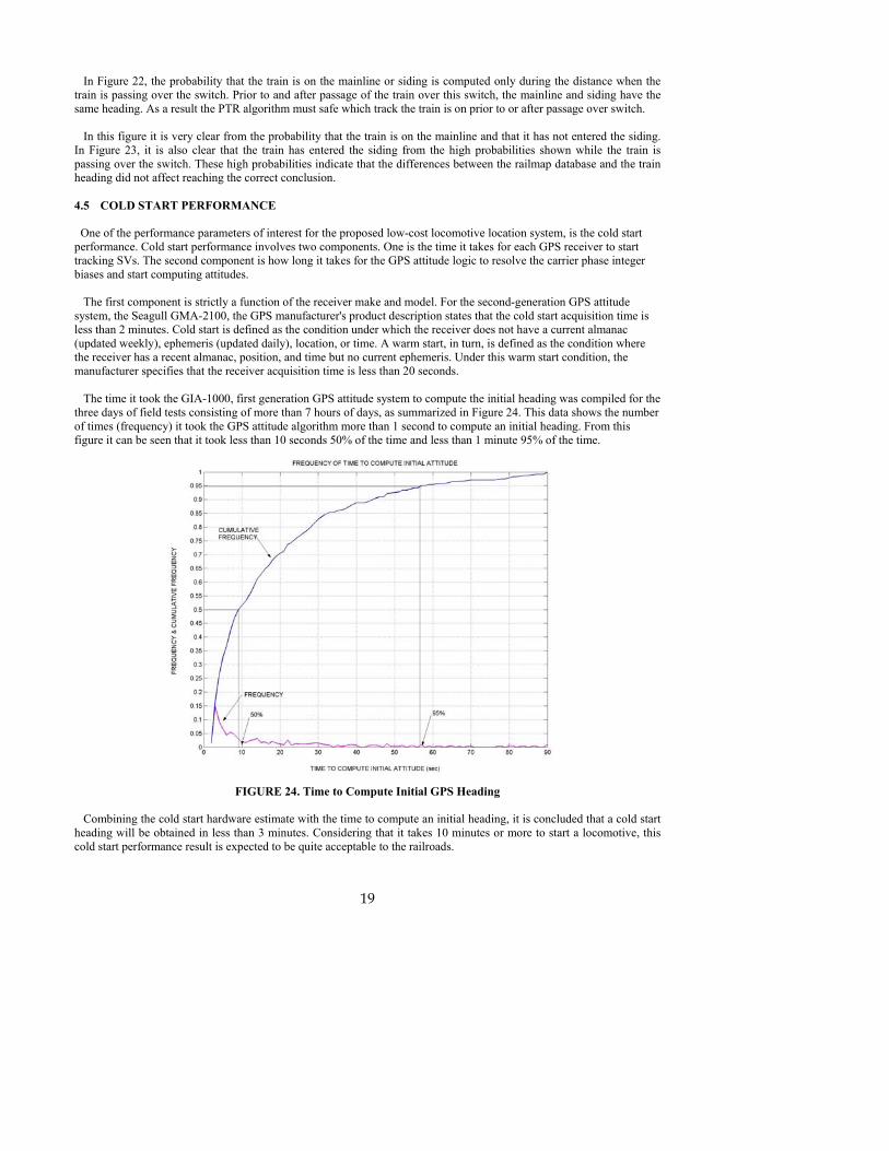
In Figure 22, the probability that the train is on the mainline or siding is computed only during the distance when the train is passing over the switch. Prior to and after passage of the train over this switch, the mainline and siding have the same heading. As a result the PTR algorithm must safe which track the train is on prior to or after passage over switch. In this figure it is very clear from the probability that the train is on the mainline and that it has not entered the siding. In Figure 23, it is also clear that the train has entered the siding from the high probabilities shown while the train is passing over the switch. These high probabilities indicate that the differences between the railmap database and the train heading did not affect reaching the correct conclusion. 4.5 COLD START PERFORMANCE One of the performance parameters of interest for the proposed low-cost locomotive location system, is the cold start performance. Cold start performance involves two components. One is the time it takes for each GPS receiver to start tracking SVs. The second component is how long it takes for the GPS attitude logic to resolve the carrier phase integer biases and start computing attitudes. The first component is strictly a function of the receiver make and model. For the second-generation GPS attitude system, the Seagull GMA-2100, the GPS manufacturer's product description states that the cold start acquisition time is less than 2 minutes. Cold start is defined as the condition under which the receiver does not have a current almanac (updated weekly), ephemeris (updated daily), location, or time. A warm start, in turn, is defined as the condition where the receiver has a recent almanac, position, and time but no current ephemeris. Under this warm start condition, the manufacturer specifies that the receiver acquisition time is less than 20 seconds. The time it took the GIA-1000, first generation GPS attitude system to compute the initial heading was compiled for the three days of field tests consisting of more than 7 hours of days, as summarized in Figure 24. This data shows the number of times (frequency) it took the GPS attitude algorithm more than 1 second to compute an initial heading. From this figure it can be seen that it took less than 10 seconds 50% of the time and less than 1 minute 95% of the time.

FIGURE 24. Time to Compute Initial GPS Heading

Combining the cold start hardware estimate with the time to compute an initial heading, it is concluded that a cold start heading will be obtained in less than 3 minutes. Considering that it takes 10 minutes or more to start a locomotive, this cold start performance result is expected to be quite acceptable to the railroads.

20

5.0 PLANS FOR IMPLEMENTATION

This study has demonstrated the feasibility of a low-cost locomotive location system for PTR using a GPS attitude system. This feasibility was demonstrated by recording data in the field and post-processing it in the laboratory. In addition, some of the key software components have been designed and tested using the field test measurements. These software algorithms include the heading Kalman filter (Appendix A) and the PTR algorithm (Appendix B). Currently, these algorithms operate in a post-processing mode. Hence, they will need to be converted to real-time operation before being embedded into a true product, namely, the GPS Locomotive Location System. 5.1 PHASE 2 PROTOTYPE DEVELOPMENT

The next logical step in the implementation of the GPS Locomotive Location System is to assemble a working, real-time prototype of the system and determine how well it performs in the field under operational conditions. The prototype would incorporate the components of Seagull's second-generation GPS multi-antenna attitude system that is currently under development for general vehicular navigation and control markets. The Kalman filter and PTR algorithm would be enhanced into practical robust algorithms for the location system processor, and converted to run in real time, as opposed to a post-processing mode. While the use of the lateral position for parallel track resolution was not investigated under this study, it is the intent to include this data in our Phase 2 prototype system. Hence, the PTR algorithms will not only use the GPS heading but also the lateral position information to achieve an exceptionally high reliability system without any additional hardware.

The proposed Phase 2 Prototype Development activity would get extensive “leverage” from Seagull’s internal GPS

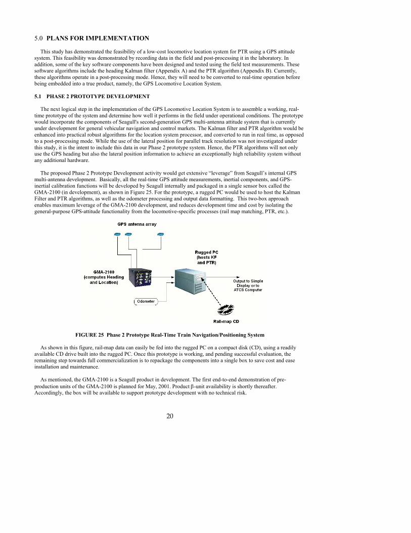
multi-antenna development. Basically, all the real-time GPS attitude measurements, inertial components, and GPS-inertial calibration functions will be developed by Seagull internally and packaged in a single sensor box called the GMA-2100 (in development), as shown in Figure 25. For the prototype, a rugged PC would be used to host the Kalman Filter and PTR algorithms, as well as the odometer processing and output data formatting. This two-box approach enables maximum leverage of the GMA-2100 development, and reduces development time and cost by isolating the general-purpose GPS-attitude functionality from the locomotive-specific processes (rail map matching, PTR, etc.).

FIGURE 25 Phase 2 Prototype Real-Time Train Navigation/Positioning System

As shown in this figure, rail-map data can easily be fed into the rugged PC on a compact disk (CD), using a readily available CD drive built into the rugged PC. Once this prototype is working, and pending successful evaluation, the remaining step towards full commercialization is to repackage the components into a single box to save cost and ease installation and maintenance.

As mentioned, the GMA-2100 is a Seagull product in development. The first end-to-end demonstration of pre-production units of the GMA-2100 is planned for May, 2001. Product β-unit availability is shortly thereafter. Accordingly, the box will be available to support prototype development with no technical risk.

21

5.2 PRODUCT COMMERCIALIZATION

Upon successful development and evaluation of the prototype system described in the previous section, the next step is to repackage the system into a convenient form for commercialization. A successfully developed prototype will offer Seagull a number of options for commercialization. One option is to identify an industry partner who can modify the prototype for mass production and has the resources and experience for marketing and distributing the GPS Locomotive Location System.

Alternatively, the prototype hardware concept and software can be licensed by companies who have the

manufacturing, distribution, and marketing organizations as well as the associated resources to bring this prototype system to market. Another option is a mixture whereby Seagull could provide the GMA-2100 and an industry partner could license the train-specific portion of the design (i. e., the software, designs and intellectual property realized in the rugged PC of Figure 24). The manufacturer can then combine this technology into one of its own product offerings.

Since the end user for this locomotive navigation system is the railroad, the railroads will select a systems integrator to perform the full PTR system installation. The systems integrator will then perform the installation based on specifications defined by the railroads. Since the Seagull GPS Locomotive Location System, defined under this study, is only one part of such a PTR system, the end customer for the Seagull is the PTR systems integrator. The key railroad systems integrators include GE-Harris, WAB Tech, and Lockheed-Martin, in addition to European railroad systems integrators. Hence, it is prudent for Seagull to strongly consider these favored system integrators in its commercialization plans.

In parallel with the proposed Phase 2 Prototype Development, Seagull intends to conduct a commercialization study to

determine a commercialization plan for the product. The commercialization plan will examine the market opportunity, necessary price points, competition, potential manufacturing and distribution partners, and other commercialization factors. Seagull will contribute the effort necessary to perform this commercialization planning as a “matching funds” activity out of its own overhead, contingent upon funding of a Phase 2 effort.

22

6.0 CONCLUSIONS This study has investigated the feasibility of a hardware and software design that will provide a low-cost drift free highly accurate and robust locomotive location system that can be used for HSR applications. Field test measurements established a raw (unfiltered) heading accuracy for this design of 0.18 degrees (1 sigma). Using a simple Kalman filter that combines low-cost heading rate gyro measurements with the GPS heading measurements, increased the heading accuracy to 0.16 degrees (1sigma). Since the PTR heading accuracy specifications require an accuracy of 0.20 degrees (1 sigma), the hardware and software design has met these requirements. In addition to the heading Kalman filter, a simple PTR algorithm was developed. This algorithm takes the train heading and path distance traveled and compares this to a railmap database. The railmap database identifies where switches are located that lead to sidings or crossovers between mainlines. When the train approaches one of these switches, the PTR algorithm determines the probability that the train continues on the original track or switches onto another track. This algorithm was also demonstrated with field data. While the field data did not include a high-speed switch (Type 20), it did establish with 0.99999 confidence the location of the train on a siding for a slower speed switch (Type 11), despite errors in the railmap database. To determine whether a GPS heading system augmented with a simple heading rate gyro is sufficient for this HSR design, a full GPS attitude system (pitch, yaw, roll) augmented with three rate gyros (pitch, yaw, roll) was used to obtain the field measurements. A Kalman filter was also written to process these six measurements. When a comparison was made between the heading estimate obtained with the 6-state Kalman filter and with a simple 2 state Kalman filter, the same heading results were obtained. As a result, it is concluded that the simple GPS heading system augmented with a low-cost heading rate gyro using a 2-state Kalman filter is sufficient for this application. It was originally thought that the train GPS velocity might be used as another source of train heading together with the GPS heading and rate gyro measurements. Due to the high accuracy achieved without the GPS velocity-derived heading, it was decided that this measurement was not required. It was also originally thought that train path distance would have to be obtained using DGPS position data. In addition, it was thought that this position data would have to be combined with the train odometer system to calibrate the odometer and filter the GPS position data. Since Selective Availability (SA) was removed from the GPS signal in 2000, the raw GPS position accuracy appears to be sufficient for this HSR application. Instead of a path distance Kalman filter, the locomotive odometer scale factor would be calibrated in the railyard by comparing the odometer to the GPS velocity derived path distance. Once calibrated, the odometer would only need to be reset periodically (while the train is stationary and waiting for a clearance to proceed) to the GPS velocity-derived path distance. While no specific test was performed to show that the GPS heading has little or no drift, unlike a gyro-based heading, the field data that was presented clearly shows that the heading has a random scatter about the measured heading. A small heading bias may be introduced when the GPS antennas are installed on the locomotive cab roof. This bias can be determined from a railyard calibration test with the train moving along a long straight track and used as a correction. While the need for a DGPS position and velocity has been minimized, the field measurements indicated long periods when the DGPS corrections from the US Coast Guard marine beacon system could be received. This addresses a concern that the electromagnetic environment generated by the locomotive turbines might produce too much interference for the reception of these corrections. As detailed in Section 5, it is recommended that the next step is to take the hardware design that was evaluated under this study and build a prototype HSR GPS locomotive location system. Also, the Kalman filter and PTR algorithms would be added to this prototype system. The prototype system would then be taken into the field to determine if it can perform to the HSR requirements in real time. REFERENCES [1] Anon, "Differential GPS: An Aid to Positive Train Control," Federal Railroad Administration, pp. 6-7, June 1995

23

7.0 INVESTIGATOR PROFILE 7.1 K. TYSEN MUELLER, Sr. Research Engineer, Seagull Technology, Inc. MA Physics California State University, Long Beach, CA 1971 BS Physics Purdue University, West Lafayette, IN 1963

Tysen Mueller is a versatile applied physicist with strong analytical skills and modeling experience. He has more than 35 years experience as a systems engineer in the areas of guidance, navigation, and computer simulation, including Kalman filtering. In addition, he has more than ten years of experience as a product and program manager in GPS/Inertial (GPS/INS) and Differential GPS (DGPS) systems. This experience includes applications to the design, development, and evaluation of Automatic Vehicle Location Systems (AVLS) and Wide Area DGPS (WADGPS) networks. He is also the co-author of a patent (June 94) on WADGPS network technologies. At Seagull Technology, he designed, developed, and delivered two real-time WADGPS correction codes: the GPS Clock Correction Code and the Ionospheric Delay Correction Code for a commercial L-Band WADGPS network. He has provided system engineering consulting support to Hughes Aircraft for the development of the FAA’s Wide Area Augmentation System (WAAS) and for the Japanese MTSAT Augmentation System (MSAS). While at Trimble Navigation, he helped define and direct the initial development of the Trimble AVLS product line as acting AVLS product manager. As program manager for the NASA Phase II SBIR Worldwide DGPS network contract, he defined the system specifications, software specifications, and test plan, and performed a survey of orbit error estimation algorithms and ionospheric delay models. For this contract, he also defined a new real-time GPS orbit error estimation algorithm and a unique global ionospheric delay model for which a patent has been granted. 7.2 SEQUOIA INSTRUMENTS DIV., Seagull Technology, Inc. The Sequoia Instruments Division of Seagull Technology has two attitude and heading reference system (AHRS) product lines. Each uses technology that enables the accurate dynamic determination of roll, pitch, and heading (among other states) using low-cost inertial technologies. It does so by complementing those sensors with external references, such as GPS, magnetometry, and/or air data. 7.2.1 Single-Antenna GPS / Inertial – GIA-2000 The model GIA-2000 Air Data Attitude and Heading Reference System (ADAHRS) complements inertial sensors with a magnetometer, GPS, and an air data computer. Motivated primarily by piloted aviation and uninhabited aerial vehicles (UAVs) applications, it is well suited for dynamic vehicle applications in magnetically clean environments. For this product line we are pursuing applicable FAA Technical Standard Order (TSO) approvals (e.g. C4c Bank and Pitch Instruments and C6d Direction Instruments, Magnetic) targeted for CY01. We are successfully completing an extensive flight validation phase that has included rigorous airborne testing by several air frame manufacturers, major avionics companies, and a FAA Aircraft Certification Office (ACO). 7.2.2 Multi-Antenna GPS / Inertial – GIA-1000 and GMA-2100 Our model GIA-1000 Attitude and Heading Reference System (AHRS) complements inertial sensors with multi-antenna GPS using a differential carrier phase approach. Magnetic information is not used. With this technology, the GPS alone provides a non-drifting and independent source of bank, pitch, and heading to complement the inertial sensors. This GPS/Inertial technology was developed prior to the GIA-2000 and is the subject of a November 1999 Avionics News cover article, in which a prototype is depicted. Although we no longer offer the GIA-1000 for sale, we are developing a second-generation multi-antenna GPS/Inertial attitude and heading reference system called the GMA-2100. Our first end-to-end demonstration of pre-production units is planned for mid-February, 2001. Product β-unit availability is expected in Spring, 2001. We have patents pending on the applicable technological innovations. The Patent and Trademark Office has approved all key claims on two applicable patents. Our technology enables performance with low-cost sensors that would otherwise require significantly more expensive sensors (e.g. that meet more demanding bias stability requirements over temperature) using traditional strap-down methods.

24

APPENDIX A: GPS HEADING KALMAN FILTER The gyro measurement is used as the source of the heading state equation:

ψωψ nGyro +=& (A-1) Since the gyro has a bias error of unknown value, an additional state equation is:

GyroGyro δωωω += (A-2)

Substituting (A-2) into (A-1): ψδωωψ nGyro ++=& (A-3) Rearranging (A-3), ( ) ψδωωψψδ nGyro +=−≡ && (A-4) The gyro heading rate error in (A-2) is assumed to be a bias error:

ωωδ nGyro =& (A-5) Hence, combining (A-4) and (A-5):

+

=

ω

ψ

δωδψ

ωδψδ

n

n, ,

GyroGyro 0010

&

& (A-6)

where, error angle and angle heading=δψψ , error (bias) rate gyro and rate, heading gyro rate, heading true=GyroGyro δωωω ,, error noise (process) whiterate gyro and heading=ωψ nn , A review of the power spectral density of the GPS heading and the gyro yaw rate measurements determined that there is a random error present in the measurement with a frequency of approximately 0.3 Hz. This is illustrated for the heading in Figure A-1.

FIGURE A-1. GPS Heading Power Spectral Density and Confidence Interval during Straight Track Yard Test

As a result, (A-6) was modified with two reciprocal time constants, βψ and βω:

+

−

−=

ω

ψψ

δωδψ

ωδψδ

n

n

β,

, β

GyroωGyro 0

1

&

& (A-7)

25

Using the GPS heading, the measurement equation is: GPSGPS m+= ψψ (A-8)

The error in the measurement of (A-8) is:

[ ] GPSGyro

GPS m+

=

δωδψ

δψ 0,1 (A-9)

The Kalman filter is based on combining the predicted (modeled) and measured values of a state vector in an optimal (minimum variance) way. Rewriting (A-7) and (A-9):

[ ] nxFx += δδ & (A-10) [ ] mxHz += δδ (A-11)

where,

≡

Gyrox

δωδψ

δ (A-12)

[ ]

−

−≡

ωβ,

, βF

01

ψ (A-13)

[ ]

≡

ω

ψ

n

nN (A-14)

[ ] [ ] 0,1≡H (A-15)

The corresponding equations for estimate of δx and δz: [ ] xFx ˆˆ δδ =& (A-16) [ ] xHz ˆˆ δδ = (A-17)

A discrete form of (A-16) is obtained as follows: ( ) [ ] ( )+

−−

−Φ=

1ˆˆ 1, kkxx kk δδ (A-18)

where, [ ] ( )[ ]nk

n

kkkk F

ntt

10

11, ! −

∞

=

−− ∑ −

=Φ (A-19)

Also, from (A-1), the discrete estimated state prediction equations are: ( ) ( )+

−−+−

− −+= 11)(1

)( ˆˆˆ kkkkk tt ωψψ (A-20)

and, )(1

)( ˆˆ +−

− = kk ωω (A-21) The estimated state correction is:

( ) ( ) ( )

+

=

+

+

−

−

+

+

k

k

k

k

k

k

ωδ

ψδ

ω

ψ

ω

ψ

ˆ

ˆ

ˆ

ˆ

ˆ

ˆ )()()(

(A-22)

or equivalently, ( ) ( ) ( )+−+ +=

kkkxxx ˆˆˆ δ (A-23)

Then the Kalman filter update is obtained: ( ) ( ) [ ] [ ] ( ){ } −−+ −+=

kkkxHzKxx kk ˆˆˆ δδδδ (A-24)

where, [ ] [ ]( )[ ] [ ][ ]( )[ ] [ ]{ } 1−−− +≡ RHPHHPK Tk

Tkk (A-25)

[ ]( ) [ ] [ ]( ) [ ] [ ] 111, 1, −+−−

− +ΦΦ=− k

Tkkkk QPP

kk (A-26)

or, [ ]( ) [ ] [ ] [ ]{ }[ ]( )−+ −= kkk PHKIP (A-27)

with, [ ] ( ) [ ]n1=n

= JnttQ

nkk

k ∑∞

−−!

1 (A-28)

[ ] [ ] [ ] [ ] [ ]( ) [ ] [ ]NJJFJFJ =1 with,+= T1-n1-k1-n1-kn (A-31)

where, [K] = Kalman gain matrix [P] = Estimation error covariance matrix [N], [Q] = Continuous and discrete process noise matrix [R] = Measurement noise matrix

26

APPENDIX B: PARALLEL TRACK RESOLUTION LOGIC The track geometry near a switch is illustrated in Figure B-1. This figure shows that the train resolution problem is formulated in a path distance-heading (s-ψ ) coordinate system. The railmap database indicates the location of a switch and shows either with discrete nodes connected by linear segments (dashed line) or turnout type (e.g.: Number 20 turnout = 1/20 radian turnout) the angle that the turnout makes. Note that the figure also includes the actual curved turnout with a solid line.

FIGURE B-1. Switch Geometry To quantify whether a train is entering a siding (to the left) or is still on the main line consider the logical decision function:

( )( ) ( )

≤≤

+≤<−+

=

otherwise (False), and,

0.50.5 if, (True), SS

0

901

0 f

mo

m

S sssLψψψψψ

(B-1)

Equation (B-1) states that the train is entering the siding if the current heading is less than the average of the main line and switch headings. The lower limit has been set to 90 degrees from this average heading since the heading would spin around if allowed to go to minus infinity. In addition, the current path distance of the train must also be between the start (point of switch) of the switch and the end (point of frog) of the switch. If the switch is to the right, then the train is entering the siding if the current heading is greater than the average heading of the switch and the main line. Use of the average of the switch and main line heading allows for uncertainties in the knowledge of the train heading as well as the switch and main line heading angles. If the heading and path distance are in error, the expected value (mean) of the logical decision function is required. In this case:

( ) ( )∫∫∞

∞−

∞

∞−

= ψψψµ ψ dsfsLds sSLS,, (B-2)

In (B-2), fsψ is the probability density function describing for the errors in s and ψ. Substituting (B-1) into (B-2):

( )( )

( )

∫∫+

−+

=MS

MS

f

Sdsfds s

s

sL

ψψ

ψψψ ψψµ

5.0

905.0

,0

(B-3)

The probability density function in (B-3) can be described by a Gaussian probability density function:

27

( )( )( )( ) ( )

−+

−−

=2

2

2

2

22

21, s

sss

s

essf σµ

σ

µψ

ψ

ψ

ξ

σπσψ (B-4)

where, s, ψ = path distance and heading, with path distance serving as the independent variable µ, σ = mean and standard deviation f = probability density Substituting (B-4) into (B-3):

( ) ( )

( )

( )

= ∫∫

+

−+

−−−

− MS

MS

f

s

s

Sdedse

s

s

s

sL

ψψ

ψψ

σ

µψ

ψ

σµ

ψσπσπ

µ ψ

ξ5.0

905.0

22 2

2

0

2

2

21

21 (B-5)

Equation (B-5) can be evaluated using the error function:

( ) ∫ −≡x

y dyxerf e0

22π

(B-6)

Using (B-6) to evaluate (B-5):

( ) ( )

−−+−

−+

−−

−=

2

905.0

2

50

2225.0 0

ψ

ψ

ψ

ψ

σ

µψψ

σ

µψψ

σ

µ

σ

µµ MSMS

S

s

S

sfL erf

.erf

serf

serf

S (B-7)

To implement this algorithm in real time, the current estimates for the train path distance and heading are used in place of the mean values for these variables. Hence (B-7) is replaced with:

( ) ( ) ( ) ( ) ( ) ( ) ( )

( ) f

MSMS

SS

fL

stss

terf

terf

tsserf

tsserft

S

<<

−−+−

−+

−−

−=

ˆ

,2

ˆ905.02

ˆ5.02

ˆ

2

ˆ25.0

0

0

for,

ψψ σ

ψψψ

σ

ψψψ

σσµ

(B-8)

The estimates for the train path distance, heading, path distance standard deviation, and heading standard deviation are obtained as outputs of the path distance and the heading Kalman filters, or equivalent algorithms.