- 1 -

Article published in Structure and Infrastructure Engineering

(post-print version)

Long-term monitoring and assessment of a precast

continuous viaduct

Helder Sousa, Carlos Sousa, Afonso S. Neves, João Bento, Joaquim Figueiras

http://www.tandfonline.com/doi/abs/10.1080/15732479.2011.614260?tab=permissions#tabModule

Article published online: 19 SEP 2011

DOI:10.1080/15732479.2011.614260

Copyright © 2013 Taylor & Francis

Structure and Infrastructure Engineering

Volume 52, pages 777–793, August 2013

- 2 -

Long-term monitoring and assessment of a precast continuous viaduct

Helder Sousaa,*

, Carlos Sousaa, Afonso S. Neves

a, João Bento

b, Joaquim

Figueirasa

a LABEST, Faculty of Engineering, University Porto

b BRISA – Auto-Estradas de Portugal S. A.

Corresponding author: Helder Sousa; LABEST, Faculty of Engineering, University

Porto, Rua Dr. Roberto Frias s/n, 4200-465 Porto, Portugal; Tel.: +351225081823; fax:

+351225081835; e-mail: mail@hfmsousa.com

Precast girders have recently been widely employed in the construction of bridges and

viaducts. The new bridge over the Tagus River in Portugal, the Lezíria Bridge,

comprehends a 9160 m long South Approach Viaduct, which was built with precast girders

made continuous in situ. Given the relevance of this construction, a long-term monitoring

system was implemented and measurements were taken since the start of the construction.

The observed parameters were concrete strains and temperatures, deck rotations, joint

displacements, accelerations and also environment temperature and relative humidity.

The work presents the precast structure, the monitoring system, and the appraisal of a

statistical procedure for the long-term assessment of the structural behaviour. This

procedure is based on prediction models, which establish the normal correlation patterns

between environmental and material parameters (such as concrete temperature and

shrinkage strains), and the observed structural response in terms of strains, rotations and

movements of expansion joints. The calculation of the normal correlation pattern

comprehends the minimization of a square error. By applying the prediction model to the

structural response measured in the South Approach Viaduct of the Lezíria Bridge, it was

found that this methodology is a feasible tool for real-time damage detection of bridges.

Keywords: Precast concrete bridges, long-term monitoring, numerical validation prediction

models, correlation patterns.

1. Introduction

Structural monitoring is an issue that receives more and more research interest and

Bridge Health Monitoring Systems (BHMS) have been a subject of increasing

international relevance. While in the past attention was focused on sensors, the

emphasis is shifting to the practical implications regarding the acquisition, collecting

and processing of data (Van der Auweraer and Peeters 2003). Today it is possible to

continuously and remotely monitor highly instrumented structures, with a high degree

of automation. Present solutions are versatile enough to allow for surveillance tasks to

- 3 -

be remotely carried out in a cost effective manner (Bergmeister and Santa 2001; Chang,

et al. 2009).

The condition assessment of a given structure may be performed by comparing

monitoring results against numerical models that describe the predicted structural

behavior. Finite Element models (FEM) have been widely employed in those

calculations. FEM make it possible to calculate the long-term behavior of bridge

structures, considering the influence of concrete creep and shrinkage, temperature and

imposed loads. Accurate estimates of the actual structural behavior can only be obtained

if the relevant concrete properties (creep, shrinkage and modulus of elasticity) are

determined through adequate tests and the real temperature history is known. However,

this information is not always available. Moreover, the detailed analysis through FEM,

considering the real sequence of construction, is a time consuming process.

An alternative approach for condition assessment consists in using the data

collected by the monitoring systems to establish the statistical models which describe

the normal correlation pattern between non-structural parameters (such as temperature

and shrinkage strains) and the observed structural response (strains, rotations and

movements of expansion joints). Some authors have already followed this path. Indeed,

the long-term monitoring of the Cogan and Grangetown viaducts (UK) were studied by

Howells et al. (Howells, et al. 2005) and Barr et al. (Barr, et al. 1997). These authors

found that a linear relationship could be established between the observed strains and

temperatures, although these temperatures differ slightly, depending on the season and

the segment location within the span. Ni et al. (Ni, et al. 2007) have also analyzed the

relationship between observed temperatures and bridge response. However, unlike the

former, whose study was based on environmental temperatures, Ni et al. used

temperatures measured inside the bridge cross sections. This enabled the authors to

- 4 -

establish a normal correlation pattern between temperatures and structural response. The

correlation model was used to establish alarms to detect future monitoring data that

disobey the normal pattern. In this authors’ study, the analysis of the structural response

was focused on the movement of the expansion joints, envisioning the scheduled

interval for replacement of expansion joints.

The long-term behavior of structures such as the South Approach Viaduct of the

Lezíria Bridge, in Portugal, is complex. In fact, it is well known that significant stress

redistributions occur over the service life, due to concrete creep and shrinkage

deformations and the evolution of the structural system during the construction phases.

Therefore, a monitoring system was implemented to follow the structural behavior since

the beginning of the construction.

In this paper, the above mentioned structure is briefly described and the

implemented monitoring system is presented. Then, the main steps involved in the

treatment of the experimental data are exposed.

At that stage, the comparison between the experimental results and the outcome

of FE models is addressed. It was concluded that FE models are able to provide

approximate estimates of the long-term behavior if detailed information about the

material properties and the construction procedure are available. However, the analysis

procedure is time consuming and the FE results hardly match the observed values with a

high degree of accuracy, because the definition of the material properties, the

environmental parameters, the structure geometric characteristics and the applied loads

always involve some degree of approximation.

Therefore, a real time assessment procedure was developed to calculate the

expected value of the monitored parameters at a given time. The developed approach is

based on prediction models, which establish the normal correlation patterns between

- 5 -

non-structural parameters and the observed structural response. That correlation pattern

is established in the first years after construction, assuming that the structure has a

healthy behavior in that period. For later ages, the expected values can then be

compared with the observed ones, so that anomalies can be detected if the difference

exceeds a given threshold limit. One of the strengths of this methodology lies in the fact

that it provides quick calculation results with minimum time and computational efforts.

Moreover, it is suitable for implementation in automatic monitoring systems, which

trigger an alarm if unexpected values occur. In this context, this work aims at

contributing to the development of systems devoted to the management and

maintenance of bridges.

2. The precast viaduct

The Lezíria Bridge, a, 11,670m long structure, is composed of three distinct

substructures: (i) the north approach viaduct; (ii) the main bridge crossing the Tagus

River; (iii) and the longest one, the south approach viaduct, with a total length of

9160m. The south approach viaduct is a partially precast structure and is composed of

22 elementary viaducts, whose total length (i.e., distance between expansion joints)

ranges from 250m to 530m. The most common span length is 36m.

Each elementary viaduct is composed of a continuous deck monolithically

connected to the piers. The foundation is provided by piles, which have the same cross

section as the piers, thus forming a pier-pile element. Transition piers were adopted to

establish the connection between the different elementary viaducts. In the transition, one

of the elementary viaducts is connected to the transition pier by means of fixed pot

bearings whereas the other is supported by sliding guided bearings.

The deck slab, which is 29.95m wide, is made up of four 1.75m high, precast, U-

shaped girders and a 0.25m thick slab. The girders are prestressed by means of

- 6 -

pretension strands and were made in a factory specifically build at the construction site.

The prestress release was carried out approximately 12 hours after casting.

The slab is composed of precast planks and a cast-in-place layer. The monolithic

connection between spans is established through a cast-in-place diaphragm and

continuity reinforcement. Moreover, in the region above the piers, the deck slab is

prestressed by straight post-tensioning cables. The continuity diaphragm is also

monolithically connected to the piers, which have a circular cross section and a diameter

of 1.5m. On the top of the pier, there is an octagonal capital whose maximum dimension

reaches 1.7m, so that the girders can be positioned without conflicts with the pier

reinforcement. In the transverse direction, a precast beam connects the capitals of each

two pillars. The piles cross alluviums with variable constitution, and the maximum

deepness reached by each pile varies between 35m and 60m. The concrete piles were

cast inside steel tubular elements, which were installed by using a vibratory pile

hammer (COBA-PC&A-CIVILSER-ARCADIS 2006).

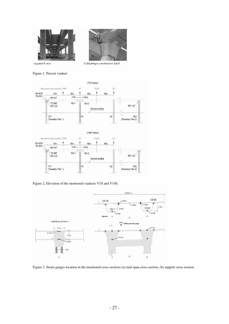
Fig. 1 depicts an image of the viaduct construction and a detail of the continuity

diaphragm during construction.

3. The monitoring system

The decision to monitor this structure was motivated by two main reasons. Firstly, it is a

very long structure, made with a repetitive precast solution; consequently, the actual

performance of the structural solution can be observed by monitoring part of the

structure; in this way, the bridge owner can be aware of the long-term structure

performance, spending a reduced value with respect to the overall structure cost.

Secondly, important stress redistributions occur in these structures, due to the employed

construction sequence and the concrete creep and shrinkage properties. Therefore, the

- 7 -

monitoring results of this complex behavior are expected to provide valuable data for

the validation of a proper numerical model.

Two out of the 22 elementary viaducts were monitored: the V1S and the V14S

(Fig. 2). Before the start of the construction, a monitoring plan was developed, which

indicates the parameters of interest and the critical cross sections that were selected for

monitoring (Figueiras, et al. 2007). These viaducts were extensively instrumented,

namely with vibrating wire strain gauges to measure concrete deformations (CD),

thermistors and resistive temperature detectors to measure concrete temperature (CT),

inclinometers to measure girder rotations about the horizontal axis of the deck cross

section (RO), linear variable differential transformers to measure the longitudinal

relative displacement between the deck and the supports at the sliding guided bearings

(BD) as well as temperature and humidity sensors to measure environmental conditions

(TE, RH). Fig. 2 presents the elevation of the monitored viaducts, with indication of the

cross sections in which embedded sensors were installed, as well the external sensors

location, while Fig. 3 illustrates the distribution of the embedded sensors in two typical

cross sections: mid-span and support cross sections. Some of the embedded sensors are

labeled in Fig. 3 for future reference in the paper.

Eight concrete prisms, with dimensions 15 cm ⋅ 15 cm ⋅ 55 cm, were cast for

measurement of shrinkage deformations. These prisms were instrumented with strain

gauges and temperature sensors and subjected to the same curing conditions of the

monitored structural elements, to achieve as a realistic representation as possible, of the

deck concrete shrinkage. Four prisms were made with girder concrete and subjected to

the curing procedure applied to the precast beams; the other ones were made with slab

concrete (from the mid-span region of the second span). For each concrete composition,

half of the prisms were subjected to the surrounding environmental conditions (although

- 8 -

sheltered from rain), whereas the others were kept in the interior of the box girder since

the pouring of the second-span slab of each viaduct.

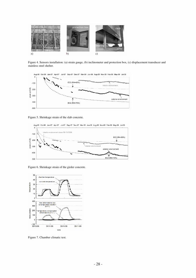
Given the aggressiveness of the concreting operations, the embedded sensors

(vibrating wire strain gauges and temperature sensors) were fixed to the reinforcement,

near the concrete surface, by using square steel bars, which allowed a robust installation

(Fig. 4-a). In general, measurements started before the concreting operations.

Consequently, it was necessary to install cables through provisory and safe paths and

acquisition systems in adequate protection boxes, to prevent potential damage due to the

construction works. The available time for these works was always short. For that

reason, the installation of all the embedded sensors was a demanding task. The bridge

deck instrumentation comprised two main phases: (i) the instrumentation of the precast

girders, which started in the precast plant; (ii) the instrumentation of the deck slab,

which started before the in situ concreting.

The external sensors were installed after the structure was cast. Inclinometers

with great inertial sensitivity were employed to measure the deck rotation about the

horizontal axis. These sensors were rigidly attached to a metallic base, which was

previously fixed to the precast girder surface and properly leveled (Fig. 4-b). The

metallic base is provided with a mechanism allowing the leveling of the sensor without

removing it. Both temperature and humidity sensors were installed in two different

environments: (i) inside the box girders; (ii) outside the precast girders, sheltered from

rain. Given that it is not possible to access the interior of the box girders after the end of

the construction, internal sensors were fixed to a movable sealed device, so that the

sensors could be accessed in case of malfunctioning or for maintenance operations.

Linear Variable Differential Transformers (LVDTs) were installed to monitor the

bearing displacements of the viaducts. These sensors were installed after the expansion

- 9 -

joint was placed. The installation was made by fixing one sensor end to the pier top, and

the other to the lateral face of the girder that is supported by sliding guided bearings. In

order to prevent damage and to guarantee the appropriate mechanical protection, all the

external sensors were encapsulated in a protection box (ventilated in the case of the

environmental parameters measuring). In the case of the LVDT, the mechanical

protection was performed by a stainless steel shelter (Fig 4-c).

4. Interpretation of concrete strains

A large number of vibrating wire strain gauges were employed to evaluate concrete

strains. The results obtained with these sensors must be carefully interpreted. According

to Eq. (1), the strain reading, obtained by direct correlation with the wire vibration

frequency, may be decomposed into three basic components: (i) the instantaneous

deformations that occur at specific instants of time, t0, caused by events such as

loadings or prestressing operations, εci(t0); (ii) the delayed deformation due to long term

effects such as creep and shrinkage, εcs+cc(t); the deformation due to temperature

variations, εcT(t0).

)()()()( 0 tttt cTcccs

i

cic εεεε ++= +∑ (1)

4.1. Instantaneous deformations

If the cause of a given instantaneous deformation, εci(t0), is not known, then it is not

possible to interpret correctly the corresponding results. This is even more complicated

in a structure that was built across different construction phases. For this reason,

information about all the relevant construction events was recorded and compiled in the

quality control report (TACE 2007). This document allows the identification of the

construction event that matches a given instantaneous deformation.

- 10 -

4.2. Time-dependent deformations

The time-dependent deformations are mainly due to the concrete creep and shrinkage.

The relaxation of prestressing steel is also responsible for long-term deformations,

however both the magnitude and the variability of this phenomena are significantly less

important than those due to creep and shrinkage. In this context, shrinkage was measure

in eight prisms, as mentioned before.

Figs. 5 and 6 depict the monitored strains in the shrinkage prisms of the V14S

viaduct without the temperature effect (analogous results were obtained in the other

monitored viaduct). In these two figures, the shrinkage estimated according to the

Eurocode 2 (European Committee 2004) is also shown, and it was based on the concrete

compressive strength measured in cubes (TACE 2007), considering a notional cross-

section size of 150 mm, and taking into account the fact that the concrete is made of

high strength rapid hardening cements. Two different values were considered for the

relative humidity (RH=70% and RH=90%), which correspond to the average observed

values in the exterior and interior environments. These figures show that the shrinkage

prisms provide relevant information to support the interpretation of the monitoring

results, as the code estimates do not precisely follow the observed values:

• even though the Eurocode 2 estimates might yield similar results for both concretes,

there are significant differences between the actual shrinkage development in both

materials, due to their different compositions and curing conditions;

• the girder concrete exhibits high shrinkage values in the first days after casting,

which is not observed in the slab concrete, for which the Eurocode 2 overestimates

the deformations;

• the observed shrinkage curves exhibit a seasonal variation, which has already been

detected by other authors (Santos 2002; Santos 2007); shrinkage increases in the

warm and dry months and decreases in the winter, but, again, this effect is not taken

into account by the code estimates.

4.3. Temperature effect on deformations

- 11 -

Sensors used to measure concrete deformations are influenced, in general, by concrete

temperature variation. Vibrating wire strain gauges are sensitive to both the wire and the

concrete temperatures. Therefore, these sensors are usually provided with an internal

thermistor, so that the temperature influence can be taken into account. The concrete

strain can thus be obtained through the following equation:

( ) ( ) TkffGFtc ∆⋅+−⋅=2

1

2

2ε (2)

where GF is the sensor gauge factor, f1 and f2 represent the initial and the actual

(at the time t) vibrating wire frequency respectively and ∆T is the temperature variation.

If the total concrete deformation is to be obtained, then only the wire temperature-

dependent deformation must be compensated. In this case, the parameter k takes the

value:

wirek α= (3)

where αwire represents thermal dilation coefficient of the wire. The manufacturer

usually gives this value and it takes the value 11 µε/ºC for the sensors used in this work

(Gage Technique International). However, it is often more convenient to obtain a strain

reading which does not include the free thermal deformation. This can be achieved by

taking the following parameter k:

( )cwirek αα −= (4)

where αc represents the thermal dilation coefficient of the concrete. If the

temperature compensation is carried out in this way, then the obtained strain εc(t) only

includes stress dependent deformations (i.e., deformations caused by concrete stresses)

and shrinkage strains. The strain obtained through this compensation procedure is

suitable for comparison with the results of numerical models.

The accurate evaluation of the temperature effect depends on the correct

estimate of the parameter αc. For this reason, a set of prisms (made with the same

- 12 -

concrete that was used in the structure and instrumented with the same type of

transducer) was tested in a climatic chamber. The test procedure consisted in applying

different temperature cycles. The temperature variation was slow, so that a uniform

temperature distribution could be obtained in the prisms. The temperature ranged from 5

ºC to 40 ºC, which broadly corresponds to the range of temperatures observed in the

structure. The results obtained for the parameter ( )cwirek αα −= that eliminates the

sensitivity to the free thermal deformation are characterized by an average value µ =

3.1 µε/ºC and a standard deviation σ2 = 0.09 µε2

/ºC2 (Sousa and Figueiras 2009). Fig. 7

presents the results obtained in one typical concrete prism. The evolution of both the

concrete temperature and the climatic chamber temperature is also represented in this

figure. These results reveal that the thermal dilation coefficient of the employed

concrete is approximately equal to 7.9 µε/ºC. This value is similar to that obtained by

other authors (Santos 2007; Kada, et al. 2002).

5. Comparison between monitoring and FEM results

A finite element analysis of the V14S viaduct was carried out, aiming at evaluating

whether a detailed numerical model could provide similar results to the ones that were

experimentally obtained. A good agreement between field measurements and FEM

results validates the monitoring procedures and encourages the effective use of this

information in surveillance and assessment tasks. Two different analyses were

performed: (i) a time-dependent phased analysis of the viaduct response, comprising

both construction and service phases; (ii) a linear-elastic analysis of the structural

behavior during the proof load test.

The time-dependent analysis was carried out through a FEM with beam

elements. A phased analysis was performed, in which the actual construction sequence

was modeled, according to the recorded sequence of construction events (TACE 2007).

- 13 -

In this analysis, the constitutive model adopted to describe the concrete behavior allows

for the consideration of the creep, shrinkage and cracking effects. The definition of the

material properties was also based on the information collected during the quality-

control procedures (TACE 2007). Furthermore, the shrinkage variation was described

by curves that were determined through a curve fitting procedure based on the results of

the shrinkage prisms. Given that no creep measurements were available, the strain

results observed in one of the precast girders before its erection was used to obtain

additional information regarding the long-term behavior of the girder concrete. This was

carried out by means of a retro-analysis procedure.

A 3D FEM with brick elements was used to analyze the local behavior of the

connection between the deck and the piers during the proof load test. This is a zone of

strong geometric discontinuity. Consequently, the strains that were monitored in this

region (see Figs. 2 and 3) cannot be directly compared with results calculated by means

of finite element beam models. Furthermore, modeling the whole viaduct with 3D brick

elements would give rise to a complex and large model. Consequently, the following

analysis strategy was adopted. The global analysis of the different load cases was

carried out by a FEM with beam elements. Then, the local 3D model was used to

determine the strains in the sensor locations when the corresponding cross section is

subjected to a given bending moment. Note that the local 3D model comprises half a

span, so that the boundary conditions can be properly simulated.

This paper presents some relevant and illustrative results. A comprehensive

description of the employed numerical models and the obtained results can be found

elsewhere (Sousa, et al. 2009; Sousa, et al. 2011).

5.1. Short-term analysis (proof load test)

- 14 -

Four different load positions were considered in the proof load test to maximize the

stresses in each monitored cross section.

Fig. 8 depicts the results of the proof load testing for the 12 sensors that are

located at upper level in the 4 monitored support cross sections. The calculated results

are also plotted in this figure (note that the dashed lines do not correspond to the exact

variation of strain between points; they are only represented to clarify the interpretation

of the results). From the analysis of this figure, one may conclude that the strain

distribution through the deck slab is not uniform. This is a consequence of both the

geometric discontinuity due to the support diaphragm and the shear lag effects, which

lead to lower strains in the transducer located on the symmetry axis. In Fig. 8, this effect

is evident in both the experimental and the numerical results. Moreover, there is a

remarkable agreement between the calculated and the observed results and a good

repeatability of measurements in corresponding locations.

5.2. Long-term analysis

Fig. 9 presents the strain results for one of the monitored mid-span cross sections,

during the construction and the first years in service. Some relevant construction stages

are identified in this figure and the observed values (at 6 a.m.) are represented by

symbols that identify the location of each point. Note that measurements started before

the precast girder was cast and the strain values do not include the free thermal

deformation.

This figure also depicts the results of two FEM analyses: (i) continuous lines

represent calculations in which the concrete properties were based on monitored

parameters (results of concrete cube tests, shrinkage measurements and retro-analyses

for identification of the creep properties) (Sousa, et al. 2011), and (ii) dashed lines

present the outcome of calculations in which the concrete properties are based on the

- 15 -

Eurocode 2 estimates and the design specifications. Figs. 5 and 6 had already shown

that the measured shrinkage deformations were significantly different from the code

estimations. Therefore, it is not surprising that calculations based on estimated concrete

properties lead to results significantly different from the observed ones. Differences are

particularly important in the first weeks after casting the precast girder and before

casting the continuity connection, because the deviation between the actual creep and

shrinkage deformations and the estimated values are significantly higher in this period.

In the long term, the agreement between measurements and calculations is improved,

namely in the case of the girder strains. In the case of the deck slab, important

differences exist even in the long term, because the actual slab shrinkage strains are

lower than the estimated values (see Fig. 5).

Conversely, the outcome of the detailed analysis with concrete properties based

on measured parameters closely agrees with the observed strains. Therefore, important

conclusion could be taken from the calibrated FEM analyses: they revealed that the

actual structure behavior is in accordance with the expected response, and the good

agreement and correlation between the different measured parameters gives confidence

in the monitoring system. FEM analyses proved to be relevant for validation of the

measured values. However, detailed analyses are time-consuming and a lot of detailed

information is necessary for the accurate calculation of the long-term structure response.

Thus, the use of simpler approaches for real-time long-term assessment of the structure

performance is encouraged and justified.

6. Prediction models

6.1. Model description

A possible approach for real time assessment of the structure condition was evaluated

within the scope of the present work. This procedure consists in obtaining the normal

- 16 -

correlation pattern between the structural response (strains, rotations and movements of

expansion joints) and basic information provided by environmental and material

parameters (such as concrete temperature and concrete shrinkage measurements). If the

new structure has a healthy behavior in the first years after construction, it is possible to

determine the normal correlation pattern between different measurements. These

correlations can be regarded as prediction models, which can be used to assess the

adequacy of the structure behavior in the future.

The proposed model is described by Eq. (5), where the model prediction ymodel(t)

for a given parameter (strains, rotations or movements of expansion joints) at a given

time t is estimated from a linear combination of measurements xmeasure,i(t) weighted by

wi. The predictor parameters xmeasure,i(t) must comply with the following conditions: (i)

the structure response must be sensitive to the value of this parameters; (ii) they must

not depend on the soundness of the structure behavior, i.e., they must represent material

properties or environmental characteristics; (iii) minimal correlation should exist

between the predictor parameters. It is desirable that these parameters correlate highly

with the dependent ones, but the existence of high correlation between the predictors

(multicollinearity) leads to imprecise determination of the coefficients wi, inaccurate

estimates and inexact tests on the regression coefficients (Montgomery and Runger

2003). In this work, the predictor parameters consist of concrete temperature and

concrete shrinkage measurements, for the reason that these variables strongly affect the

time variation of the structure response.

ε+=

⋅=∑=

)()(

)()(

modelmeasure

1

,measuremodel

tyty

txwtyk

i

ii

(5)

- 17 -

The problem unknowns consist of the set of weights wi. The problem is solved

by calculating the value of the weights wi which minimize the differences, ε, between

the actual measurement ymeasure(t) and the model prediction, ymodel(t). The optimal

solution is the one that minimizes the function R, which represents the sum of the

squared errors, as represented by Eq. (6). The minimum of the function R is found by

setting the gradient to zero. This problem has an unique solution because R is a

quadratic function, ymodel(t) being a linear combination of a set of measurements.

( )

kjw

R

tytyR

kwww

j

n

i

i

n

i

i

n

i

ielimeasure

,...,2,10

)()(

,...,,

1

2

min

1

2

1

2

mod

10

==∂

∂

⇒

=−=

∑

∑∑

=

==

ε

ε

(6)

The observation period (i.e., the set of times ti) over which the minimization

problem is formulated must also be established. In this type of problems, it is common

to use a fraction of the total available period of observation, a so called “training

window”. The appropriate size of the training window can be determined by making

several calculations with increasingly larger dimensions. The adequate time window is

the one that lead to the same set of weights wi that would be obtained if larger training

windows were considered.

It is worthy of note that the size of the training window depends on the

phenomena under analysis. If the prediction model is devised for long-term structural

analyses, then a minimum size of one year might be necessary, for the reason that the

concrete temperatures and delayed deformations have a seasonal variation with a yearly

period.

Once the set of weights is determined, the model may be used to calculate the

expected structure response ymodel(t) for the remaining time window. If the structure has

- 18 -

a normal behavior, the magnitude of the error ε shows the robustness of the prediction

model.

This algorithm was implemented in an existing software devoted to structural

monitoring – MENSUSMONITOR. Its user-friendly interface and capacity to connect

to MySQL databases enabled efficient data handling and simple calculation procedures.

More details about this tool can be found elsewhere (Sousa, et al. 2008).

6.2. Application to the precast viaduct

6.2.1. Problem description

The prediction model was used to analyze the outcome of 24 transducers (12 from

viaduct V1S and 12 from V14S): 4 (2+2) bearing displacements BD; 4 (2+2) deck

rotations RO; and 16 (8+8) concrete deformations CD, of four mid-span cross sections

(Figs. 2 and 3). The predictor parameters xmeasure,i(t) were shrinkage deformations SD

observed in concrete prisms and concrete temperatures CT. Fig. 10 shows the location

of the temperature sensors, which are positioned in three mid-span cross sections.

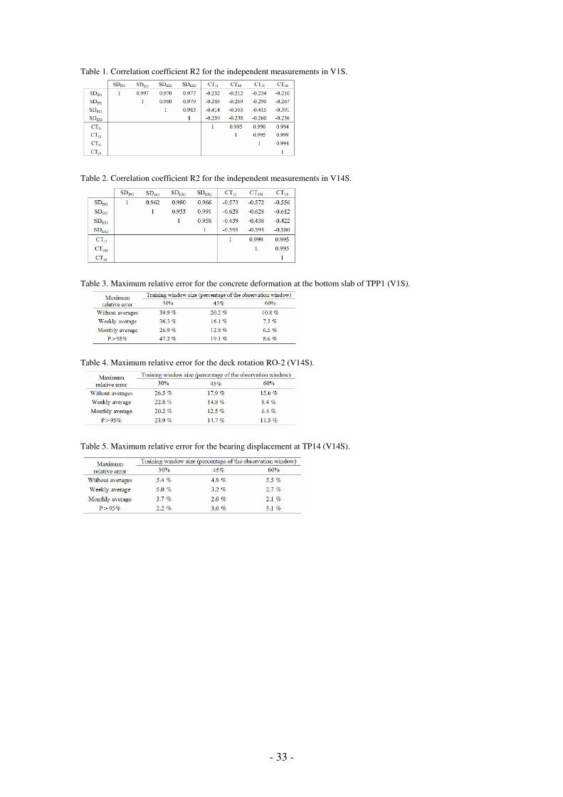
Tables 1 and 2 present the correlation coefficients R2 for all the measurements

that are candidates to be used as predictor parameters, for viaducts V1S and V14S

respectively. These tables show that high correlation exists within the subsets of

temperatures and shrinkage measurements, with R2 always higher than 0.95. This

indicates a strong collinearity between measurements of each data set. Consequently,

instability problems would occur in the calculation of the problem unknowns (the set of

weights wi) if more than 1 temperature and 1 shrinkage strain were taken as predictor

parameters.

Therefore, only two independent variables were considered: the average of the

shrinkage deformations SDAVG and the average of the concrete temperatures CTAVG.

The correlation coefficients between these variables are -0.281 and -0.542 for viaducts

- 19 -

V1S and V14S, respectively. These correlations lead to Variance Inflation Factors of

1.1 and 1.4, respectively, which are clearly lower than 10 (the threshold value for

multicollinearity) and robust model predictions can thus be achieved (Montgomery and

Runger 2003). In this way, the prediction model given by Eq. (5) is expressed by Eq.

(7).

)()()( 21mod tCTwtSDwty AVGAVGel ⋅+⋅= (7)

The uniform depth of this bridge deck and the reduced thickness of both the

deck slab and the girders justify the adoption of such a simple description of the

temperature influence as presented in Eq. (7). However, in structures composed by

thicker elements higher temperature gradients occur, which requires a more detailed

definition of the temperature influence.

For this study, the observation period ranges from 24-12-2007 to 05-10-2009,

with one sample per day, at 6h a.m.

6.2.2. Results and discussion

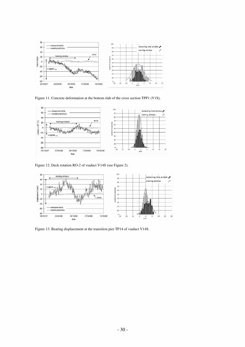
Figs. 11 to 13 present the model predictions for three measurements: a concrete

deformation, a deck rotation and a bearing displacement. For each measurement, the

first graph depicts the time variation of measured values and model predictions. The

training window size was taken as one year, which corresponds to 60% of the complete

time range. However, the influence of this size is discussed below. The time variation of

the error ε, i.e., the difference between measurements and model predictions, is also

depicted in the graph. A second graph for each measurement shows histograms of the

calculated errors, for both the training window and the remaining time window. The

Gaussian distribution that best fits these histograms is also plotted.

The quality of the predictions for the different measurements can be compared

by using the relative error concept, which is defined as the ratio between the calculated

- 20 -

error at a given time t and the range of variation of measurements over the complete

time window (see e.g. Fig. 11). It was observed that the smallest relative errors occur in

the case of the bearing displacement. For this parameter, the maximum relative error is

4.6%, and 95% of the calculated errors are lower than 3.2%. Moreover, the error

average takes the value 0.45 mm, which corresponds to 0.5% of the signal amplitude.

This small value reveals that the models prediction follows the actual measurements and

the error has a random nature. The correlation coefficient between predictions and

measurements equals 0.99, which confirms a good correlation.

The poorest performance of the prediction model was observed in the deck

rotation, for which the maximum relative error is 20.3%. However, even in this case, the

error mean is approximately equal to zero. As for the concrete deformation, the

maximum error takes the value 10.8%. It is not surprising that the best agreement

between measurements and predictions occur in the case of the bearing displacement.

This is a global measurement that is influenced by the deformation of a large portion of

the structure. Therefore, a good correlation between this parameter and the average

values of temperature and shrinkage measurements was expected. On the other hand,

local measurements such as concrete deformations are very sensitive to the local

concrete behavior, which does not correlate so well with the adopted average predictor

parameters.

The occurrence of errors is also justified by the fact that the structure response is

also sensitive to other variables that were not considered as predictor ones: traffic

loading, wind, insolation, rainfall, among others with minor importance. This is why the

prediction of the deck rotations was the poorest one: this transducer is the most sensitive

to traffic loadings. However, the fact that the mean error is approximately equal to zero

shows that the adopted predictor variables play a key role in the long-term structure

- 21 -

response. If the long-term performance is to be evaluated, then it is logical to analyze

the average error over a certain period, so that the relevance of random deviations due to

the ignored effects is reduced. Tables 3 to 5 display the maximum relative error for

weekly and monthly averages, showing that the error significantly decreases if averaged

values are taken into account. The most significant reduction occurs for the deck

rotation when the training window is equal to 60% of the observation window, a fact

that is justified by the aforementioned reasons.

6.2.3. Discussion of the training window size

Tables 3 to 5 show the variation of the maximum relative error as the training window

size increases (taking values of 30%, 45% and 60% of the observation time window),

for the three transducers under analysis. Besides the maximum individual error and the

weekly and monthly averages, these tables also present the maximum error for a

probability of occurrence of 95%.

In general, the maximum errors decrease as the training window size increases.

In the case of the deck rotation, similar results are obtained for window percentages of

45% and 60%. As regards the bearing displacements, the training window size seems to

have a minor influence on the calculation results. The influence of the training window

size can be more clearly understood by analyzing Fig. 14, which depict the evolution of

the set of weights wi (the problem unknowns) when the training window size varies

from 1% to 100% of the total period. The figure shows that a very small training

window (~10% of the observation time) guarantees a good estimate of the weights wi

for prediction of bearing displacements. This conclusion conforms to the fact that these

global displacements are well correlated with the predictor variables: averages of the

measured concrete temperatures and shrinkage strains. On the other hand, large training

windows are required for the prediction of local concrete deformations as well as for

- 22 -

deck rotations, because of lower correlation with the predictor variables. An extensive

study was also performed for the remaining sensors and similar conclusions were

gathered.

6.2.4. Example of anomaly detection

The usefulness of the prediction model can be demonstrated by the following real

example. Fig. 15 shows the time variation of measurements and model predictions for

one of the monitored bearing displacements. The time variation of the calculated error

(difference between measurements and predictions) shows an abrupt variation at a

specific time (09-05-2008 6h a.m.), which indicates some anomaly. After searching for

possible explanations for this occurrence, it was found that this instant of time

corresponded to maintenance operations that forced a temporary removal of the LVDT.

Upon removal and replacement of the transducer, the reference was lost, which justifies

the detected deviation in the graphical representation of the error.

This maintenance operation was carried out without communication with the

authors. It could only be detected after the prediction model has been applied to the

results of this transducer. Therefore, the usefulness of the prediction model is not

restricted to the detection of structure deficiencies; it also detects anomalies in the

monitoring results.

It must be highlighted that, in this work, the occurrence of anomalies is

associated to abnormal deviations between the measured structural response and the

model estimation. The normal correlation pattern is established for a period of time in

which healthy behavior is assumed and the threshold limit is derived from the statistical

analysis of the deviations in that period of time. However, the definition of threshold

limits could be complemented with additional information based on numerical modeling

- 23 -

considering the influence of variables such as traffic, wind, insolation and rainfall. That

would be a more complex approach that is out of the scope of the present work.

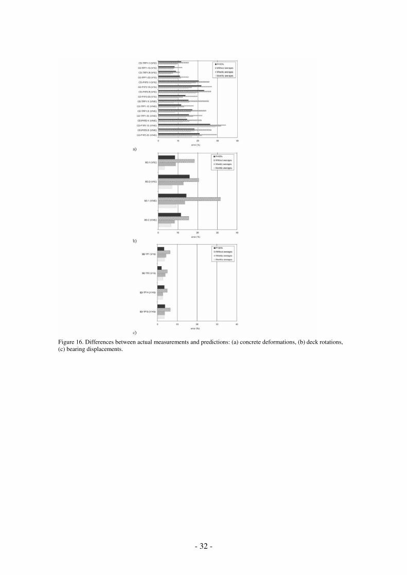
6.2.5. Global analysis of measured results

Given the large number of the installed transducers, a subset of 24 sensors was selected

for presentation in this work, as previously mentioned. Fig. 16 shows the calculated

maximum relative errors, for a training window of 60% of the total period of

observation. The label of each concrete deformation, CD, includes the cross section as

indicated in Fig. 2, the sensor location within the cross section, as shown in Fig. 3, and

the identification of the viaduct. The position of each rotation and displacement

measurements is shown in Fig. 2.

These results conform to the ones discussed before. Predictions of bearing

displacements (with maximum relative errors lower than 4% for a probability of

occurrence of 95%) are significantly better than the model estimations for concrete

deformations and deck rotations. However, it is worthy to note that the relative errors

are calculated with respect to the time variation in the observation period under analysis.

If the total range of variation was considered, then significantly lower relative errors

would be obtained. Fig. 9 shows that the maximum strain variation in the precast girder

amounts to ~850 µε. Therefore, the relative error with respect to the total range of

variation is approximately ten times lower than the one with respect to the range of

variation in the period of observation (~80 µε for the transducer in Fig. 11).

7. Conclusions

The present work focus on the monitoring and assessment of the long-term structural

behavior of continuous viaducts made with precast girders. A real structure, which was

recently built in Portugal, has been monitored since the beginning of its erection. The

- 24 -

monitoring system was carefully planned, installed and protected so that it could

provide long-term reliable results. This paper describes the viaduct, presents the

monitoring system, and discusses the procedure employed to assess the structure’s

behavior. This procedure is based on FEM calculations and regression models. Some

relevant conclusions could be drawn:

(1) The measurement of the time variation of relevant concrete properties and the

identification of the timing of the various construction events provided relevant

information for the development of accurate FE analysis. This conclusion stems

from the difference between the actual time variation of the concrete deformations

and those resulting from the design code predictions and also from the fact that the

construction sequence strongly affects the structural behavior.

(2) The good agreement between field measurements and FEM results validates the

monitoring procedures and encourages the effective use of this information in

surveillance and assessment tasks.

(3) The prediction model presented might be applied to establish normal correlation

patterns between material and environmental parameters (such as temperature and

shrinkage strains) and the observed structural response (strains, rotations and

movements of expansion joints). The problem unknowns are determined by

considering an initial time window in which healthy behavior is assumed. The

model can then be employed to calculate the expected response of the different

transducers, for each point in time. The existence of abnormal differences between

the expected values and the actual measurements reveals changes in the structural

behavior or deficiencies in the monitoring system.

(4) The choice of the predictor variables and the size of the time window used are of

relevance and their calculations were presented and discussed.

(5) The use of prediction models involves minimal time and computational efforts, if

the algorithm is implement in dedicated software, such as MENSUSMONITOR,

with direct access to the measurements database.

(6) The usefulness of the prediction model was demonstrated through a real example in

which a maintenance operation with implications in the monitoring results was

detected.

(7) The best agreement between measurements and model predictions were obtained for

transducers, which are not very sensitive to variables other than the employed

independent (i.e., predictor) variables. In this case, the best results were obtained for

the relative displacements at the expansion joints.

Acknowledgements

The authors acknowledge the support from the Portuguese Foundation for Science and Technology

through the Research Project PTDC/ECM/68430/2006 and the PhD grants SFRH/BD/29125/2006 and

SFRH/BD/25339/2005 attributed to the first and second authors. Support from the contractor consortium,

TACE, and the infrastructure owner, BRISA, is also gratefully acknowledged.

References

- 25 -

Barr, B. I. G., J. L. Vitek, and M. A. Beygi. "Seasonal Shrinkage Variation in Bridge

Segments." Materials and Structures 30, no. 196 (1997): 106-11.

Bergmeister, K., and U. Santa. "Global Monitoring Concepts for Bridges." Structural

Concrete 2, no. 1 (2001): 29 –39.

Chang, Sung-Pil, Jaeyeol Yee, and Jungwhee Lee. "Necessity of the Bridge Health

Monitoring System to Mitigate Natural and Man-Made Disasters." Structure and

Infrastructure Engineering: Maintenance, Management, Life-Cycle Design and

Performance 5, no. 3 (2009): 173 - 97.

COBA-PC&A-CIVILSER-ARCADIS. "Construção Da Travessia Do Tejo No

Carregado Sublanço A1/Benavente, Da A10 Auto-Estrada

Bucelas/Carregado/Ic3 " In Empreitada de Concepção, Projecto e Construção

da Travessia do Tejo no Carregado, 2006.

European Committee, Standardization. Eurocode 2 En 1991-1-1 Design of Concrete

Structures Part 1-1 General Rules and Rules for Buildings. Vol. 2e ed. Brussels:

CEN, 2004.

Figueiras, Joaquim, Carlos Félix, Helder Sousa, and Helena Figueiras. "Construção Da

Travessia Do Tejo No Carregado Sublanço A1/Benavente, Da A10 Auto-

Estrada Bucelas/Carregado/Ic3: Projecto Executivo Monitorização Estrutural E

De Durabilidade 0 – Apresentação." LABEST, Faculty of Engineering of the

University of Porto, 2007.

Gage Technique International, Lda "The Effect of Temperature on Vibrating Wire

Strain Gauges." United Kingdom: Gage Technique International, Lda.

Howells, R. W., R. J. Lark, and B. I. G. Barr. "A Study of the Influence of

Environmental Effects on the Behaviour of a Pre-Stressed Concrete Viaduct."

Structural Concrete 6, no. 3 (2005): 91-100.

Kada, H., M. Lachemi, N. Petrov, O. Bonneau, and P. Aïtcin. "Determination of the

Coefficient of Thermal Expansion of High Performance Concrete from Initial

Setting." Materials and Structures 35, no. 1 (2002): 35-41.

Montgomery, Douglas C., and George C. Runger. Applied Statistics and Probability for

Engineers. 3rd ed. ed: John Wiley, 2003.

Ni, Y. Q., X. G. Hua, K. Y. Wong, and J. M. Ko. "Assessment of Bridge Expansion

Joints Using Long-Term Displacement and Temperature Measurement." Journal

of Performance of Constructed Facilities 21, no. 2 (2007): 143-51.

Santos, Luís Miguel Pina de Oliveira. Observação E Análise Do Comportamento

Diferido De Pontes De Betão, Phd Thesis. Lisboa: LNEC, 2002.

Santos, Teresa Oliveira. Retracção Do Betão Em Pontes Observação E Análise. 1ª ed

ed, Phd Thesis. Lisboa: LNEC, 2007.

Sousa, C. , H. Sousa, A.S. Neves, and J. Figueiras. "Numerical Evaluation of the

Long-Term Behavior of Precast Continuous Bridge Decks." Journal of Bridge

Engineering, 10.1061/(ASCE)BE.1943-5592.0000233 (Feb. 15, 2011) (2011).

Sousa, C., H. Sousa, A. Neves, and J. Figueiras. "Finite-Element Analysis of the Long-

Term Behavior of the Precast Access Viaduct of the Leziria Bridge." LABEST,

Faculty of Engineering of the University of Porto, 2009.

Sousa, H., A. Dimande, A. Henriques, and J. Figueiras. "Mensusmonitor – Tool for the

Treatment and Interpretation of Experimental Results in Civil Engineering."

Paper presented at the CCC 2008 – Challenges for Civil Construction, FEUP -

Faculty of Engineering, University Porto, Porto, 2008.

Sousa, H., and H. Figueiras. "Experimental Evaluation of Thermal Compensation for

Vibrating Wire Strain Gauges Placed in Concrete Prisms." LABEST, Faculty of

Engineering of the University of Porto, 2009.

- 26 -

TACE. "Construção Da Travessia Do Tejo No Carregado Sublanço A1/Benavente, Da

A10 Auto-Estrada Buce-Las/Carregado/Ic3: Plano De Qualidade." 2007.

Van der Auweraer, Herman, and Bart Peeters. "International Research Projects on

Structural Health Monitoring: An Overview." Structural Health Monitoring 2,

no. 4 (2003): 341-58.

- 27 -

Figure 1. Precast viaduct.

Figure 2. Elevation of the monitored viaducts V1S and V14S.

Figure 3. Strain gauges location in the monitored cross sections (a) mid-span cross section, (b) support cross section.

- 28 -

Figure 4. Sensors installation: (a) strain gauge, (b) inclinometer and protection box, (c) displacement transducer and

stainless steel shelter.

Figure 5. Shrinkage strain of the slab concrete.

Figure 6. Shrinkage strain of the girder concrete.

Figure 7. Chamber climatic test.

- 29 -

Figure 8. Deck slab strains at the support cross sections during the load test.

Figure 9. Comparison between numerical and experimental results (strains in the mid-span cross section of the first

span, alignment B).

Figure 10. Embedded temperature sensor locations: (a) V1S-TPP1, (b) V1S-P1P2, (c) V14S-P1P2.

- 30 -

Figure 11. Concrete deformation at the bottom slab of the cross section TPP1 (V1S).

Figure 12. Deck rotation RO-2 of viaduct V14S (see Figure 2).

Figure 13. Bearing displacement at the transition pier TP14 of viaduct V14S.

- 31 -

Figure 14. Calculated weights wi as a function of the training window size: (a) concrete deformation at the bottom

slab of TPP1(V1S), (b) deck rotation RO-2 (V14S), (c) bearing displacement at TP14 (V14S).

Figure 15. Anomaly detection in bearing displacement BD-TP15 (V14S).

- 32 -

Figure 16. Differences between actual measurements and predictions: (a) concrete deformations, (b) deck rotations,

(c) bearing displacements.

- 33 -

Table 1. Correlation coefficient R2 for the independent measurements in V1S.

Table 2. Correlation coefficient R2 for the independent measurements in V14S.

Table 3. Maximum relative error for the concrete deformation at the bottom slab of TPP1 (V1S).

Table 4. Maximum relative error for the deck rotation RO-2 (V14S).

Table 5. Maximum relative error for the bearing displacement at TP14 (V14S).