logistic regression - statpower notes/logistic.pdf · logistic regression with a single predictor...
TRANSCRIPT

Logistic Regression
James H. Steiger
Department of Psychology and Human DevelopmentVanderbilt University
James H. Steiger (Vanderbilt University) Logistic Regression 1 / 38
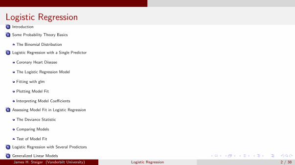
Logistic Regression1 Introduction
2 Some Probability Theory Basics
The Binomial Distribution
3 Logistic Regression with a Single Predictor
Coronary Heart Disease
The Logistic Regression Model
Fitting with glm
Plotting Model Fit
Interpreting Model Coefficients
4 Assessing Model Fit in Logistic Regression
The Deviance Statistic
Comparing Models
Test of Model Fit
5 Logistic Regression with Several Predictors
6 Generalized Linear Models
James H. Steiger (Vanderbilt University) Logistic Regression 2 / 38

Introduction
Introduction
Logistic Regression deals with the case where the dependent variable is binary, and theconditional distribution is binomial.Recall that, for a random variable Y having a binomial distribution with parameters n(the number of trials), and p ( the probability of “success” , the mean of Y is np and thevariance of Y is np(1− p).Therefore, if the conditional distribution of Y given a predictor X is binomial, then themean function and variance functions will be necessarily related.Moreover, since, for a given value of n, the mean of the conditional distribution isnecessarily bounded by 0 and n, it follows that a linear function will generally fail to fit atlarge values of the predictor.So, special methods are called for.
James H. Steiger (Vanderbilt University) Logistic Regression 3 / 38

Some Probability Theory Basics The Binomial Distribution
Some Probability Theory BasicsThe Binomial Distribution
This discrete distribution is one of the foundations of modern categorical data analysisThe binomial random variable X represents the number of “successes” in N outcomes ofa binomial processA binomial process is characterized by
N independent trialsOnly two outcomes, arbitrarily designated “success” and “failure”Probabilities of success and failure remain constant over trials
Many interesting real world processes only approximately meet the above specificationsNevertheless, the binomial is often an excellent approximation
James H. Steiger (Vanderbilt University) Logistic Regression 4 / 38

Some Probability Theory Basics The Binomial Distribution
Some Probability Theory BasicsThe Binomial Distribution
The binomial distribution is a two-parameter family, N is the number of trials, p theprobability of successThe binomial has pdf
Pr(X = r) =
(N
r
)pr (1− p)N−r
The mean and variance of the binomial are
E (X ) = Np
Var(X ) = Np(1− p)
James H. Steiger (Vanderbilt University) Logistic Regression 5 / 38

Some Probability Theory Basics The Binomial Distribution
Some Probability Theory BasicsThe Binomial Distribution
The B(N, p) distribution is well approximated by a N(Np,Np(1− p)) distribution as longas p is not too far removed from .5 and N is reasonably largeA good rule of thumb is that both Np and N(1− p must be greater than 5The approximation can be further improved by correcting for continuity
James H. Steiger (Vanderbilt University) Logistic Regression 6 / 38
Logistic Regression with a Single Predictor Coronary Heart Disease
Logistic Regression with a Single PredictorCoronary Heart Disease
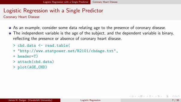
As an example, consider some data relating age to the presence of coronary disease.The independent variable is the age of the subject, and the dependent variable is binary,reflecting the presence or absence of coronary heart disease.
> chd.data <- read.table(
+ "http://www.statpower.net/R2101/chdage.txt",
+ header=T)
> attach(chd.data)
> plot(AGE,CHD)
James H. Steiger (Vanderbilt University) Logistic Regression 7 / 38
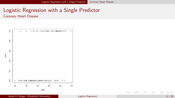
Logistic Regression with a Single Predictor Coronary Heart Disease
Logistic Regression with a Single PredictorCoronary Heart Disease
20 30 40 50 60 70
0.0
0.2
0.4
0.6
0.8
1.0
AGE
CH
D
James H. Steiger (Vanderbilt University) Logistic Regression 8 / 38
Logistic Regression with a Single Predictor Coronary Heart Disease
Logistic Regression with a Single PredictorCoronary Heart Disease
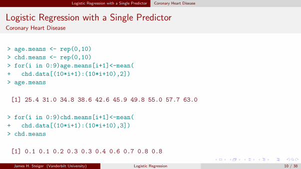
The general trend, that age is related to coronary heart disease, seems clear from theplot, but it is difficult to see the precise nature of the relationship.We can get a crude but somewhat more revealing picture of the relationship between thetwo variables by collecting the data in groups of ten observations and plotting mean ageagainst the proportion of individuals with CHD.
James H. Steiger (Vanderbilt University) Logistic Regression 9 / 38
Logistic Regression with a Single Predictor Coronary Heart Disease
Logistic Regression with a Single PredictorCoronary Heart Disease
> age.means <- rep(0,10)
> chd.means <- rep(0,10)
> for(i in 0:9)age.means[i+1]<-mean(
+ chd.data[(10*i+1):(10*i+10),2])
> age.means
[1] 25.4 31.0 34.8 38.6 42.6 45.9 49.8 55.0 57.7 63.0
> for(i in 0:9)chd.means[i+1]<-mean(
+ chd.data[(10*i+1):(10*i+10),3])
> chd.means
[1] 0.1 0.1 0.2 0.3 0.3 0.4 0.6 0.7 0.8 0.8
James H. Steiger (Vanderbilt University) Logistic Regression 10 / 38
Logistic Regression with a Single Predictor Coronary Heart Disease
Logistic Regression with a Single PredictorCoronary Heart Disease
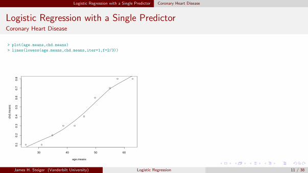
> plot(age.means,chd.means)
> lines(lowess(age.means,chd.means,iter=1,f=2/3))
30 40 50 60
0.1
0.2
0.3
0.4
0.5
0.6
0.7
0.8
age.means
chd.
mea
ns
James H. Steiger (Vanderbilt University) Logistic Regression 11 / 38
Logistic Regression with a Single Predictor The Logistic Regression Model
Logistic Regression with a Single PredictorThe Logistic Regression Model
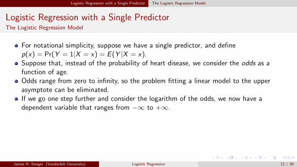
For notational simplicity, suppose we have a single predictor, and definep(x) = Pr(Y = 1|X = x) = E (Y |X = x).Suppose that, instead of the probability of heart disease, we consider the odds as afunction of age.Odds range from zero to infinity, so the problem fitting a linear model to the upperasymptote can be eliminated.If we go one step further and consider the logarithm of the odds, we now have adependent variable that ranges from −∞ to +∞.
James H. Steiger (Vanderbilt University) Logistic Regression 12 / 38
Logistic Regression with a Single Predictor The Logistic Regression Model
Logistic Regression with a Single PredictorThe Logistic Regression Model
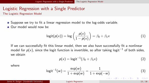
Suppose we try to fit a linear regression model to the log-odds variable.Our model would now be
logit(p(x)) = log
(p(x)
1− p(x)
)= β0 + β1x (1)
If we can successfully fit this linear model, then we also have successfully fit a nonlinearmodel for p(x), since the logit function is invertible, so after taking logit−1 of both sides,we obtain
p(x) = logit−1(β0 + β1x) (2)
where
logit−1(w) =exp(w)
1 + exp(w)=
1
1 + exp(−w)(3)
James H. Steiger (Vanderbilt University) Logistic Regression 13 / 38
Logistic Regression with a Single Predictor The Logistic Regression Model
Logistic Regression with a Single PredictorThe Logistic Regression Model
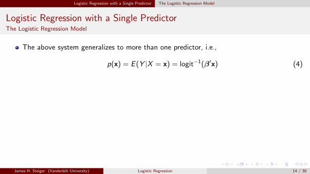
The above system generalizes to more than one predictor, i.e.,
p(x) = E (Y |X = x) = logit−1(β′x) (4)
James H. Steiger (Vanderbilt University) Logistic Regression 14 / 38
Logistic Regression with a Single Predictor The Logistic Regression Model
Logistic Regression with a Single PredictorThe Logistic Regression Model
It turns out that the system we have just described is a special case of what is nowtermed a generalized linear model.In the context of generalized linear model theory, the logit function that “linearizes” thebinomial proportions p(x) is called a link function.In this module, we shall pursue logistic regression primarily from the practical standpointof obtaining estimates and interpreting the results.Logistic regression is applied very widely in the medical and social sciences, and entirebooks on applied logistic regression are available.
James H. Steiger (Vanderbilt University) Logistic Regression 15 / 38
Logistic Regression with a Single Predictor Fitting with glm
Logistic Regression with a Single PredictorFitting with glm
Fitting a logistic regression model in R is straightforward.You use the glm function and specify the binomial distribution family and the logit linkfunction.
James H. Steiger (Vanderbilt University) Logistic Regression 16 / 38
Logistic Regression with a Single Predictor Fitting with glm
Logistic Regression with a Single PredictorFitting with glm
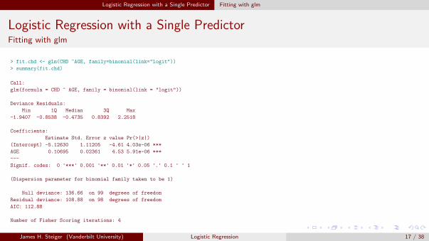
> fit.chd <- glm(CHD ~AGE, family=binomial(link="logit"))
> summary(fit.chd)
Call:
glm(formula = CHD ~ AGE, family = binomial(link = "logit"))
Deviance Residuals:
Min 1Q Median 3Q Max
-1.9407 -0.8538 -0.4735 0.8392 2.2518
Coefficients:
Estimate Std. Error z value Pr(>|z|)
(Intercept) -5.12630 1.11205 -4.61 4.03e-06 ***
AGE 0.10695 0.02361 4.53 5.91e-06 ***
---
Signif. codes: 0 '***' 0.001 '**' 0.01 '*' 0.05 '.' 0.1 ' ' 1
(Dispersion parameter for binomial family taken to be 1)
Null deviance: 136.66 on 99 degrees of freedom
Residual deviance: 108.88 on 98 degrees of freedom
AIC: 112.88
Number of Fisher Scoring iterations: 4
James H. Steiger (Vanderbilt University) Logistic Regression 17 / 38
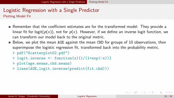
Logistic Regression with a Single Predictor Plotting Model Fit
Logistic Regression with a Single PredictorPlotting Model Fit
Remember that the coefficient estimates are for the transformed model. They provide alinear fit for logit(p(x)), not for p(x). However, if we define an inverse logit function, wecan transform our model back to the original metric.Below, we plot the mean AGE against the mean CHD for groups of 10 observations, thensuperimpose the logistic regression fit, transformed back into the probability metric.
> pdf("Scatterplot02.pdf")
> logit.inverse <- function(x){1/(1+exp(-x))}
> plot(age.means,chd.means)
> lines(AGE,logit.inverse(predict(fit.chd)))
James H. Steiger (Vanderbilt University) Logistic Regression 18 / 38
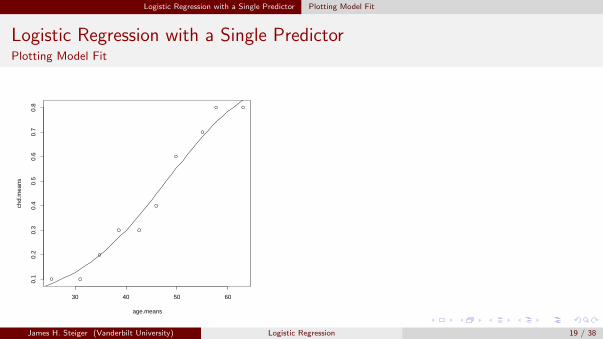
Logistic Regression with a Single Predictor Plotting Model Fit
Logistic Regression with a Single PredictorPlotting Model Fit
30 40 50 60
0.1
0.2
0.3
0.4
0.5
0.6
0.7
0.8
age.means
chd.
mea
ns
James H. Steiger (Vanderbilt University) Logistic Regression 19 / 38
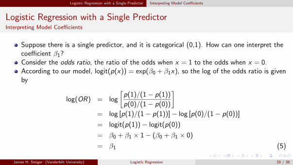
Logistic Regression with a Single Predictor Interpreting Model Coefficients
Logistic Regression with a Single PredictorInterpreting Model Coefficients
Suppose there is a single predictor, and it is categorical (0,1). How can one interpret thecoefficient β1?Consider the odds ratio, the ratio of the odds when x = 1 to the odds when x = 0.According to our model, logit(p(x)) = exp(β0 + β1x), so the log of the odds ratio is givenby
log(OR) = log
[p(1)/(1− p(1))
p(0)/(1− p(0))
]= log [p(1)/(1− p(1))]− log [p(0)/(1− p(0))]
= logit(p(1))− logit(p(0))
= β0 + β1 × 1− (β0 + β1 × 0)
= β1 (5)
James H. Steiger (Vanderbilt University) Logistic Regression 20 / 38
Logistic Regression with a Single Predictor Interpreting Model Coefficients
Logistic Regression with a Single PredictorInterpreting Model Coefficients
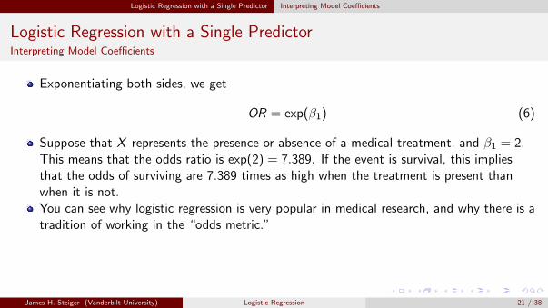
Exponentiating both sides, we get
OR = exp(β1) (6)
Suppose that X represents the presence or absence of a medical treatment, and β1 = 2.This means that the odds ratio is exp(2) = 7.389. If the event is survival, this impliesthat the odds of surviving are 7.389 times as high when the treatment is present thanwhen it is not.You can see why logistic regression is very popular in medical research, and why there is atradition of working in the “odds metric.”
James H. Steiger (Vanderbilt University) Logistic Regression 21 / 38
Logistic Regression with a Single Predictor Interpreting Model Coefficients
Logistic Regression with a Single PredictorInterpreting Model Coefficients
In our coronary heart disease data set, the predictor is continuous.Interpreting model coefficients when a predictor is continuous is more difficult.Recalling the form of the fitted function for p(x), we see that it does not have a constantslope.By taking derivatives, we compute the slope as β1p(x)(1− p(x)). Hence, the steepestslope is at p(x) = 1/2, at which x = −β0/β1, and the actual slope is β1/4.In toxicology, this is called LD50, because it is the dose at which the probability of deathis 1/2.
James H. Steiger (Vanderbilt University) Logistic Regression 22 / 38
Logistic Regression with a Single Predictor Interpreting Model Coefficients
Logistic Regression with a Single PredictorInterpreting Model Coefficients
So a rough “rule of thumb” is that when X is near the middle of its range, a unit changein X results in a change of β1/4 units in p(x).More precise calculations can be achieved with the aid of R and the logit−1 function.
James H. Steiger (Vanderbilt University) Logistic Regression 23 / 38
Logistic Regression with a Single Predictor Interpreting Model Coefficients
Logistic Regression with a Single PredictorInterpreting Model Coefficients
Example (CHD vs. AGE)
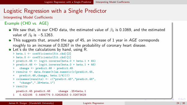
We saw that, in our CHD data, the estimated value of β1 is 0.1069, and the estimatedvalue of β0 is −5.1263.This suggests that, around the age of 45, an increase of 1 year in AGE correspondsroughly to an increase of 0.0267 in the probability of coronary heart disease.Let’s do the calculations by hand, using R.> beta.1 <- coefficients(fit.chd)[2]
> beta.0 <- coefficients(fit.chd)[1]
> predict.45 <- logit.inverse(beta.0 + beta.1 * 45)
> predict.46 <- logit.inverse(beta.0 + beta.1 * 46)
> change <- predict.46 - predict.45
> results <- data.frame(t(as.numeric(c(predict.45,
+ predict.46,change, beta.1/4))))
> colnames(results) <- c("predict.45","predict.46",
+ "change",".25*beta.1")
> results
predict.45 predict.46 change .25*beta.1
1 0.422195 0.4484776 0.02628253 0.02673629
James H. Steiger (Vanderbilt University) Logistic Regression 24 / 38
Logistic Regression with a Single Predictor Interpreting Model Coefficients
Logistic Regression with a Single PredictorInterpreting Model Coefficients
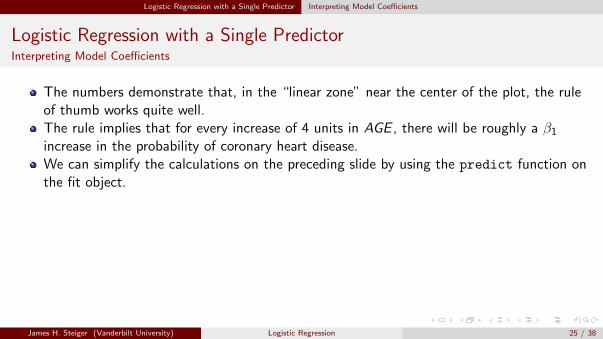
The numbers demonstrate that, in the “linear zone” near the center of the plot, the ruleof thumb works quite well.The rule implies that for every increase of 4 units in AGE , there will be roughly a β1
increase in the probability of coronary heart disease.We can simplify the calculations on the preceding slide by using the predict function onthe fit object.
James H. Steiger (Vanderbilt University) Logistic Regression 25 / 38
Logistic Regression with a Single Predictor Interpreting Model Coefficients
Logistic Regression with a Single PredictorInterpreting Model Coefficients
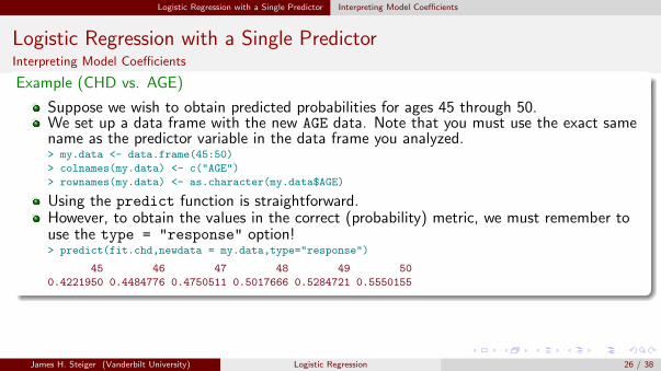
Example (CHD vs. AGE)
Suppose we wish to obtain predicted probabilities for ages 45 through 50.We set up a data frame with the new AGE data. Note that you must use the exact samename as the predictor variable in the data frame you analyzed.> my.data <- data.frame(45:50)
> colnames(my.data) <- c("AGE")
> rownames(my.data) <- as.character(my.data$AGE)
Using the predict function is straightforward.However, to obtain the values in the correct (probability) metric, we must remember touse the type = "response" option!> predict(fit.chd,newdata = my.data,type="response")
45 46 47 48 49 50
0.4221950 0.4484776 0.4750511 0.5017666 0.5284721 0.5550155
James H. Steiger (Vanderbilt University) Logistic Regression 26 / 38

Assessing Model Fit in Logistic Regression The Deviance Statistic
Assessing Model Fit in Logistic RegressionThe Deviance Statistic
In multiple linear regression, the residual sum of squares provides the basis for tests forcomparing mean functions.In logistic regression, the residual sum of squares is replaced by the deviance, which isoften called G 2. Suppose there are k data groupings based on ni , i = 1, . . . , k binomialobservations. The deviance is defined for logistic regression to be
G 2 = 2k∑
i=1
[yi log
(yiyi
)+ (ni − yi ) log
(ni − yini − yi
)](7)
where yi = ni p(xi ) are the fitted numbers of successes in ni trials in the ith grouping.The degrees of freedom associated with the analysis is the number of groupings n used inthe calculation minus the number of free parameters in β that were estimated.
James H. Steiger (Vanderbilt University) Logistic Regression 27 / 38
Assessing Model Fit in Logistic Regression Comparing Models
Assessing Model Fit in Logistic RegressionComparing Models
Comparing models in logistic regression is similar to regular linear regression.For two nested models, the difference in deviances is treated as a chi-square with degreesof freedom equal to the difference in the degrees of freedom for the two models.
James H. Steiger (Vanderbilt University) Logistic Regression 28 / 38
Assessing Model Fit in Logistic Regression Test of Model Fit
Assessing Model Fit in Logistic RegressionTest of Model Fit
When the number of trials ni > 1, the deviance G 2 can be used to provide agoodness-of-fit test for a logistic regression model.The test compares the null hypothesis that the mean function used is adequate versus thealternative that a separate parameter needs to be fit for each value of i (this latter case iscalled the saturated model).When all the ni are large enough, G 2 can be compared with the χ2
n−p distribution to getan approximate p-value.
James H. Steiger (Vanderbilt University) Logistic Regression 29 / 38
Assessing Model Fit in Logistic Regression Test of Model Fit
Assessing Model Fit in Logistic RegressionTest of Model Fit
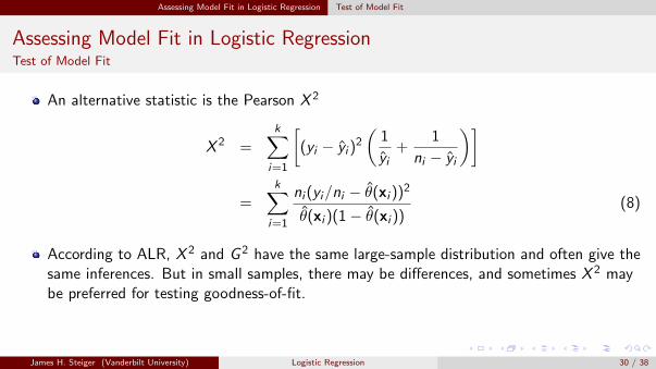
An alternative statistic is the Pearson X 2
X 2 =k∑
i=1
[(yi − yi )
2
(1
yi+
1
ni − yi
)]
=k∑
i=1
ni (yi/ni − θ(xi ))2
θ(xi )(1− θ(xi ))(8)
According to ALR, X 2 and G 2 have the same large-sample distribution and often give thesame inferences. But in small samples, there may be differences, and sometimes X 2 maybe preferred for testing goodness-of-fit.
James H. Steiger (Vanderbilt University) Logistic Regression 30 / 38
Logistic Regression with Several Predictors
Logistic Regression with Several Predictors
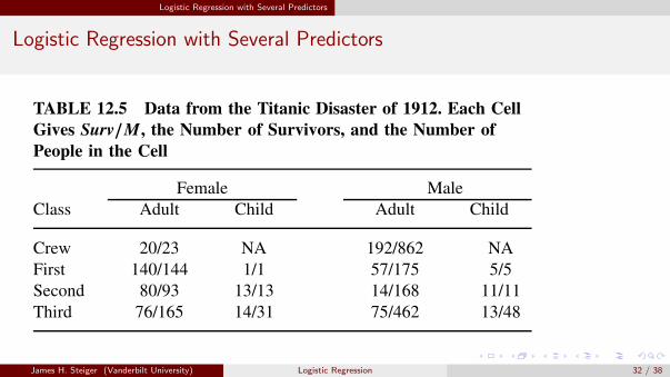
As an example of logistic predictors, Weisberg presents data from the famous Titanicdisaster. (Frank Harrell presents a much more detailed analysis of the Titanic in hissuperb book Regression Modeling Strategies).Of 2201 known passengers and crew, only 711 are reported to have survived.The data in the file titanic.txt from Dawson (1995) classify the people on board theship according to their Sex as Male or Female, Age, either child or adult, and Class,either first, second, third, or crew.Not all combinations of the three factors occur in the data, since no children weremembers of the crew. For each age/sex/class combination, the number of people M andthe number surviving Surv are also reported.The data are shown in Table 12.5.
James H. Steiger (Vanderbilt University) Logistic Regression 31 / 38
Logistic Regression with Several Predictors
Logistic Regression with Several Predictors
262 LOGISTIC REGRESSION
saturated model). When all the mi are large enough, G2 can be compared with theχ2
n−p distribution to get an approximate p-value. The goodness-of-fit test is notapplicable in the blowdown example because all the mi = 1.
Pearson’s X2 is an approximation to G2 defined for logistic regression by
X2 =n∑
i=1
[(yi − yi )
2(
1
yi
+ 1
mi − yi
)]
=n∑
i=1
mi(yi/mi − θ (xi ))2
θ (xi )(1 − θ (xi ))(12.9)
X2 and G2 have the same large-sample distribution and often give the same infer-ences. In small samples, there may be differences, and sometimes X2 may bepreferred for testing goodness-of-fit.
TitanicThe Titanic was a British luxury passenger liner that sank when it struck an icebergabout 640 km south of Newfoundland on April 14–15, 1912, on its maiden voyageto New York City from Southampton, England. Of 2201 known passengers andcrew, only 711 are reported to have survived. The data in the file titanic.txtfrom Dawson (1995) classify the people on board the ship according to their Sex asMale or Female, Age, either child or adult, and Class, either first, second, third, orcrew. Not all combinations of the three factors occur in the data, since no childrenwere members of the crew. For each age/sex/class combination, the number ofpeople M and the number surviving Surv are also reported. The data are shown inTable 12.5.
Table 12.6 gives the value of G2 and Pearson’s X2 for the fit of five meanfunctions to these data. Since almost all the mi exceed 1, we can use either G2
or X2 as a goodness-of-fit test for these models. The first two mean functions,the main effects only model, and the main effects plus the Class × Sex interac-tion, clearly do not fit the data because the values of G2 and X2 are both muchlarger then their df, and the corresponding p-values from the χ2 distribution are
TABLE 12.5 Data from the Titanic Disaster of 1912. Each CellGives Surv/M , the Number of Survivors, and the Number ofPeople in the Cell
Female MaleClass Adult Child Adult Child
Crew 20/23 NA 192/862 NAFirst 140/144 1/1 57/175 5/5Second 80/93 13/13 14/168 11/11Third 76/165 14/31 75/462 13/48
James H. Steiger (Vanderbilt University) Logistic Regression 32 / 38
Logistic Regression with Several Predictors
Logistic Regression with Several Predictors
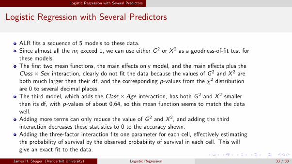
ALR fits a sequence of 5 models to these data.Since almost all the mi exceed 1, we can use either G 2 or X 2 as a goodness-of-fit test forthese models.The first two mean functions, the main effects only model, and the main effects plus theClass × Sex interaction, clearly do not fit the data because the values of G 2 and X 2 areboth much larger then their df, and the corresponding p-values from the χ2 distributionare 0 to several decimal places.The third model, which adds the Class × Age interaction, has both G 2 and X 2 smallerthan its df, with p-values of about 0.64, so this mean function seems to match the datawell.Adding more terms can only reduce the value of G 2 and X 2, and adding the thirdinteraction decreases these statistics to 0 to the accuracy shown.Adding the three-factor interaction fits one parameter for each cell, effectively estimatingthe probability of survival by the observed probability of survival in each cell. This willgive an exact fit to the data.
James H. Steiger (Vanderbilt University) Logistic Regression 33 / 38
Logistic Regression with Several Predictors
Logistic Regression with Several Predictors
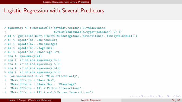
> mysummary <- function(m){c(df=m$df.residual,G2=m$deviance,
+ X2=sum(residuals(m,type="pearson")^2) )}
> m1 <- glm(cbind(Surv,N-Surv)~Class+Age+Sex, data=titanic, family=binomial())
> m2 <- update(m1,~.+Class:Sex)
> m3 <- update(m2,~.+Class:Age)
> m4 <- update(m3,~.+Age:Sex)
> m5 <- update(m4,~Class:Age:Sex)
> ans <- mysummary(m1)
> ans <- rbind(ans,mysummary(m2))
> ans <- rbind(ans,mysummary(m3))
> ans <- rbind(ans,mysummary(m4))
> ans <- rbind(ans,mysummary(m5))
> row.names(ans) <- c( "Main effects only",
+ "Main Effects + Class:Sex",
+ "Main Effects + Class:Sex + Class:Age",
+ "Main Effects + All 2 Factor Interactions",
+ "Main Effects + All 2 and 3 Factor Interactions")
James H. Steiger (Vanderbilt University) Logistic Regression 34 / 38
Logistic Regression with Several Predictors
Logistic Regression with Several Predictors
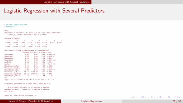
> options(scipen=1,digits=3)
> summary(m3)
Call:
glm(formula = cbind(Surv, N - Surv) ~ Class + Age + Sex + Class:Sex +
Class:Age, family = binomial(), data = titanic)
Deviance Residuals:
1 2 3 4 5 6 7 8
0.0000 0.0000 0.0000 0.0001 0.0000 0.0000 0.0000 0.0001
9 10 11 12 13 14
0.0000 0.0000 -0.8745 0.8265 0.3806 -0.3043
Coefficients: (1 not defined because of singularities)
Estimate Std. Error z value Pr(>|z|)
(Intercept) 1.897 0.619 3.06 0.0022 **
ClassFirst 1.658 0.800 2.07 0.0383 *
ClassSecond -0.080 0.688 -0.12 0.9073
ClassThird -2.115 0.637 -3.32 0.0009 ***
AgeChild 0.338 0.269 1.26 0.2094
SexMale -3.147 0.625 -5.04 4.7e-07 ***
ClassFirst:SexMale -1.136 0.821 -1.38 0.1662
ClassSecond:SexMale -1.068 0.747 -1.43 0.1525
ClassThird:SexMale 1.762 0.652 2.70 0.0069 **
ClassFirst:AgeChild 22.424 16495.727 0.00 0.9989
ClassSecond:AgeChild 24.422 13007.888 0.00 0.9985
ClassThird:AgeChild NA NA NA NA
---
Signif. codes: 0 '***' 0.001 '**' 0.01 '*' 0.05 '.' 0.1 ' ' 1
(Dispersion parameter for binomial family taken to be 1)
Null deviance: 671.9622 on 13 degrees of freedom
Residual deviance: 1.6854 on 3 degrees of freedom
AIC: 70.31
Number of Fisher Scoring iterations: 21
James H. Steiger (Vanderbilt University) Logistic Regression 35 / 38

Logistic Regression with Several Predictors
Logistic Regression with Several Predictors
> xtable(ans)
df G2 X2Main effects only 8.00 112.57 103.83
Main Effects + Class:Sex 5.00 45.90 42.77Main Effects + Class:Sex + Class:Age 3.00 1.69 1.72
Main Effects + All 2 Factor Interactions 2.00 0.00 0.00Main Effects + All 2 and 3 Factor Interactions 0.00 0.00 0.00
James H. Steiger (Vanderbilt University) Logistic Regression 36 / 38
Generalized Linear Models
Generalized Linear Models
Both the multiple linear regression model discussed earlier in this book and the logisticregression model discussed in this chapter are particular instances of a generalized linearmodel.Generalized linear models all share three basic characteristics:
James H. Steiger (Vanderbilt University) Logistic Regression 37 / 38

Generalized Linear Models
Generalized Linear Models
1 The distribution of the response Y , given a set of terms X , is distributed according to anexponential family distribution. The important members of this class include the normaland binomial distributions we have already encountered, as well as the Poisson andgamma distributions.
2 The response Y depends on the terms X only through the linear combination β′X.3 The mean E (Y |X = x) = m(β′x) for some kernel mean function m. For the multiple
linear regression model, m is the identity function, and for logistic regression, it is thelogistic function. There is considerable flexibility in selecting the kernel mean function.Most presentations of generalized linear models discuss the link function, whichtechnically is defined as the inverse of m rather than m itself.
James H. Steiger (Vanderbilt University) Logistic Regression 38 / 38