logistic regression - jbg/teaching/csci_3022/10c.pdf · pdf filelogistic regression:...

Logistic Regression

Introduction to Data Science Algorithms Jordan Boyd-Graber and Michael Paul SLIDES ADAPTED FROM WILLIAM COHEN

Introduction to Data Science Algorithms | Boyd-Graber and Paul Logistic Regression | 1 of 9

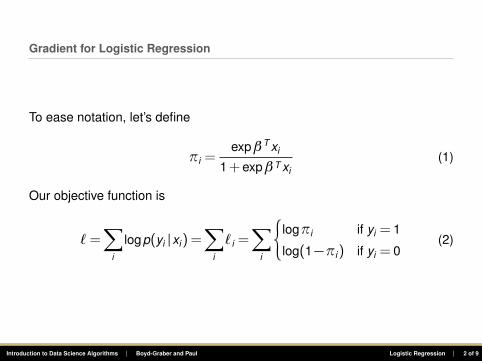
Gradient for Logistic Regression

To ease notation, let’s define

πi = expβT xi

1+expβT xi (1)

Our objective function is

`= ∑

i

logp(yi |xi) = ∑

i

`i = ∑

i

¨

logπi if yi = 1

log(1−πi) if yi = 0 (2)

Introduction to Data Science Algorithms | Boyd-Graber and Paul Logistic Regression | 2 of 9

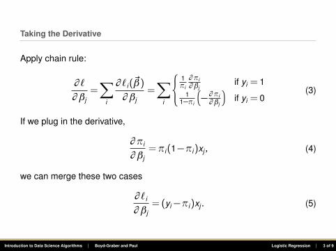
Taking the Derivative

Apply chain rule:

∂ `

∂ βj = ∑

i

∂ `i( ~β)

∂ βj = ∑

i

(

1 πi ∂ πi ∂ βj

if yi = 1 1

1−πi

− ∂ πi∂ βj

if yi = 0 (3)

If we plug in the derivative,

∂ πi ∂ βj

=πi(1−πi)xj , (4)

we can merge these two cases

∂ `i ∂ βj

= (yi −πi)xj . (5)

Introduction to Data Science Algorithms | Boyd-Graber and Paul Logistic Regression | 3 of 9

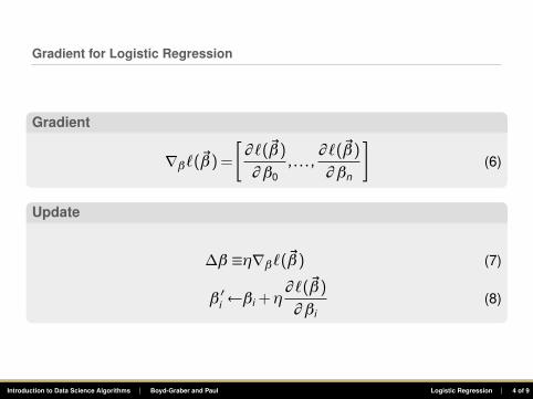
Gradient for Logistic Regression

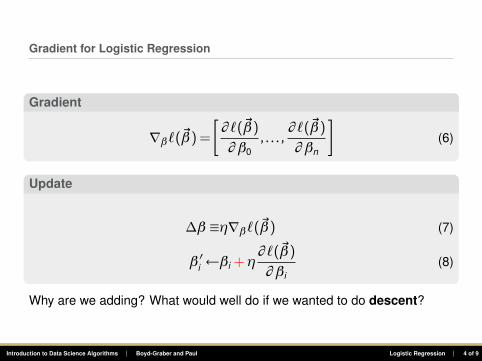
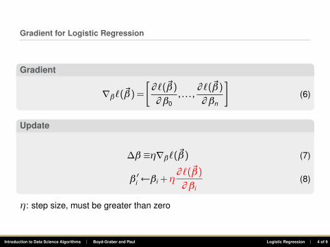
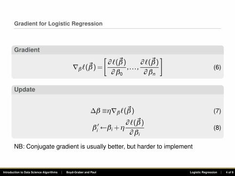
Gradient

∇β`( ~β) = �

∂ `( ~β)

∂ β0 , . . . ,

∂ `( ~β)

∂ βn

�

(6)

Update

∆β ≡η∇β`( ~β) (7)

β ′i ←βi +η ∂ `( ~β)

∂ βi (8)

Introduction to Data Science Algorithms | Boyd-Graber and Paul Logistic Regression | 4 of 9

Gradient for Logistic Regression

Gradient

∇β`( ~β) = �

∂ `( ~β)

∂ β0 , . . . ,

∂ `( ~β)

∂ βn

�

(6)

Update

∆β ≡η∇β`( ~β) (7)

β ′i ←βi +η ∂ `( ~β)

∂ βi (8)

Why are we adding? What would well do if we wanted to do descent?

Introduction to Data Science Algorithms | Boyd-Graber and Paul Logistic Regression | 4 of 9

Gradient for Logistic Regression

Gradient

∇β`( ~β) = �

∂ `( ~β)

∂ β0 , . . . ,

∂ `( ~β)

∂ βn

�

(6)

Update

∆β ≡η∇β`( ~β) (7)

β ′i ←βi +η ∂ `( ~β)

∂ βi (8)

η: step size, must be greater than zero

Introduction to Data Science Algorithms | Boyd-Graber and Paul Logistic Regression | 4 of 9

Gradient for Logistic Regression

Gradient

∇β`( ~β) = �

∂ `( ~β)

∂ β0 , . . . ,

∂ `( ~β)

∂ βn

�

(6)

Update

∆β ≡η∇β`( ~β) (7)

β ′i ←βi +η ∂ `( ~β)

∂ βi (8)

NB: Conjugate gradient is usually better, but harder to implement

Introduction to Data Science Algorithms | Boyd-Graber and Paul Logistic Regression | 4 of 9

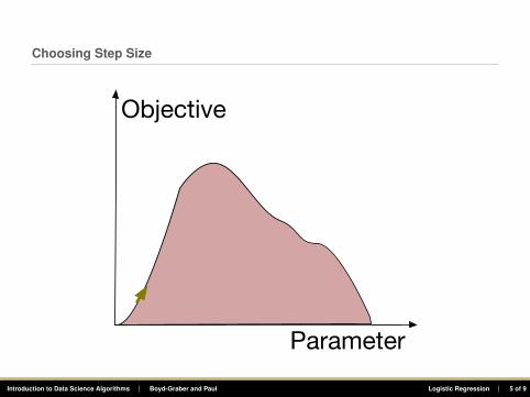
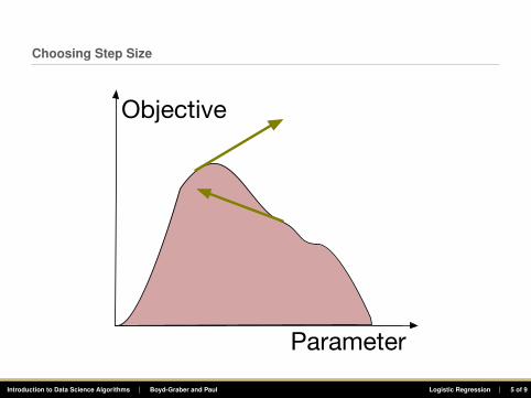
Choosing Step Size

Parameter

Objective

Introduction to Data Science Algorithms | Boyd-Graber and Paul Logistic Regression | 5 of 9

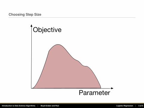
Choosing Step Size

Parameter

Objective

Introduction to Data Science Algorithms | Boyd-Graber and Paul Logistic Regression | 5 of 9

Choosing Step Size

Parameter

Objective

Introduction to Data Science Algorithms | Boyd-Graber and Paul Logistic Regression | 5 of 9

Choosing Step Size

Parameter

Objective

Introduction to Data Science Algorithms | Boyd-Graber and Paul Logistic Regression | 5 of 9

Choosing Step Size

Parameter

Objective

Introduction to Data Science Algorithms | Boyd-Graber and Paul Logistic Regression | 5 of 9

Approximating the Gradient

• Our datasets are big (to fit into memory) • . . . or data are changing / streaming

• Hard to compute true gradient

`(β)≡Ex [∇`(β ,x)] (9)

• Average over all observations • What if we compute an update just from one observation?

Introduction to Data Science Algorithms | Boyd-Graber and Paul Logistic Regression | 6 of 9

Approximating the Gradient

• Our datasets are big (to fit into memory) • . . . or data are changing / streaming • Hard to compute true gradient

`(β)≡Ex [∇`(β ,x)] (9)

• Average over all observations

• What if we compute an update just from one observation?

Introduction to Data Science Algorithms | Boyd-Graber and Paul Logistic Regression | 6 of 9

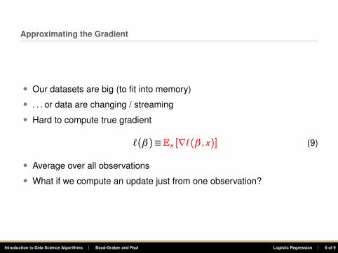
Approximating the Gradient

• Our datasets are big (to fit into memory) • . . . or data are changing / streaming • Hard to compute true gradient

`(β)≡Ex [∇`(β ,x)] (9)

• Average over all observations • What if we compute an update just from one observation?

Introduction to Data Science Algorithms | Boyd-Graber and Paul Logistic Regression | 6 of 9

Getting to Union Station

Pretend it’s a pre-smartphone world and you want to get to Union Station

Introduction to Data Science Algorithms | Boyd-Graber and Paul Logistic Regression | 7 of 9

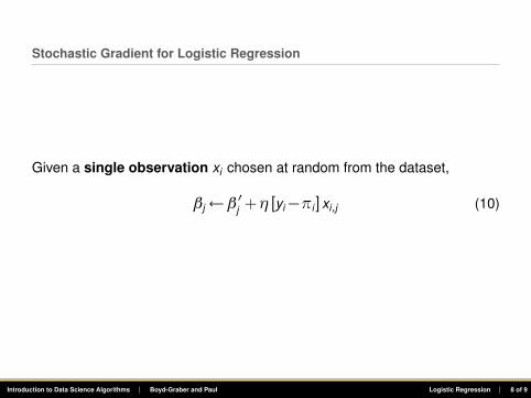
Stochastic Gradient for Logistic Regression

Given a single observation xi chosen at random from the dataset,

βj ←β ′j +η [yi −πi ]xi ,j (10)

Examples in class.

Introduction to Data Science Algorithms | Boyd-Graber and Paul Logistic Regression | 8 of 9

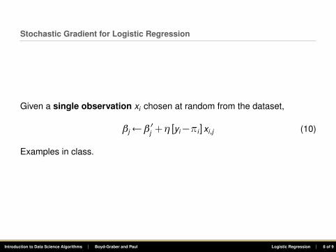
Stochastic Gradient for Logistic Regression

Given a single observation xi chosen at random from the dataset,

βj ←β ′j +η [yi −πi ]xi ,j (10)

Examples in class.

Introduction to Data Science Algorithms | Boyd-Graber and Paul Logistic Regression | 8 of 9

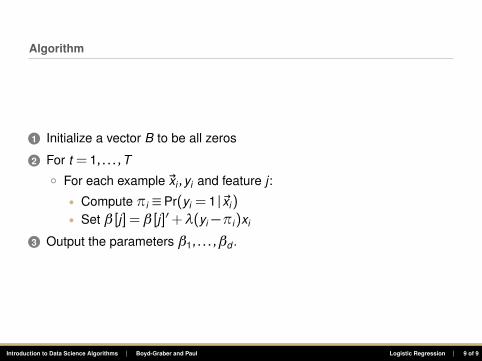
Algorithm

1 Initialize a vector B to be all zeros

2 For t = 1, . . . ,T

◦ For each example ~xi ,yi and feature j : • Compute πi ≡ Pr(yi = 1 | ~xi) • Set β [j] =β [j]′+λ(yi −πi)xi

3 Output the parameters β1, . . . ,βd .

Introduction to Data Science Algorithms | Boyd-Graber and Paul Logistic Regression | 9 of 9

Wrapup

• Logistic Regression: Regression for outputting Probabilities • Intuitions similar to linear regression • We’ll talk about feature engineering for both next time

Introduction to Data Science Algorithms | Boyd-Graber and Paul Logistic Regression | 10 of 9