NBER WORKING PAPER SERIES

LINEARITY-GENERATING PROCESSES:A MODELLING TOOL YIELDING CLOSED FORMS FOR ASSET PRICES

Xavier Gabaix

Working Paper 13430http://www.nber.org/papers/w13430

NATIONAL BUREAU OF ECONOMIC RESEARCH1050 Massachusetts Avenue

Cambridge, MA 02138September 2007

Konstantin Milbradt and Oleg Rytchkov provided very good research assistance. For helpful conversations,I thank Marco Avellaneda, John Campbell, Peter Carr, Sylvain Champonnois, George Constantinides,John Cox, Greg Duffee, Darrell Duffie, Pierre Collin-Dufresne, Alex Edmans, Ralph Koijen, FrancisLongstaff, Sydney Ludvigson, Antonio Mele, Lasse Pedersen, Monika Piazzesi, José Scheinkman,Pietro Veronesi (a discussant), and seminar participants at Carnegie-Mellon, MIT, NYU, Princeton,Urbana-Champaign, and the NBER. I thank the NSF for support. The views expressed herein are thoseof the author(s) and do not necessarily reflect the views of the National Bureau of Economic Research.

© 2007 by Xavier Gabaix. All rights reserved. Short sections of text, not to exceed two paragraphs,may be quoted without explicit permission provided that full credit, including © notice, is given tothe source.

Linearity-Generating Processes: A Modelling Tool Yielding Closed Forms for Asset PricesXavier GabaixNBER Working Paper No. 13430September 2007JEL No. E43,G12,G13

ABSTRACT

This methodological paper presents a class of stochastic processes with appealing properties for theoreticalor empirical work in finance and macroeconomics, the "linearity-generating" class. Its key propertyis that it yields simple exact closed-form expressions for stocks and bonds, with an arbitrary numberof factors. It operates in discrete and continuous time. It has a number of economic modeling applications.These include macroeconomic situations with changing trend growth rates, or stochastic probabilityof disaster, asset pricing with stochastic risk premia or stochastic dividend growth rates, and yieldcurve analysis that allows flexibility and transparency. Many research questions may be addressedmore simply and in closed form by using the linearity-generating class.

Xavier GabaixNew York UniversityFinance DepartmentStern School of Business44 West 4th Street, 9th floorNew York, NY 10012and NBERxgabaix@stern.nyu.edu

1 Introduction

This methodological paper defines and analyzes a class of stochastic processes that has a

number of attractive properties for economics and finance, the “linearity-generating” (LG)

processes. It is generates closed-form solutions for the prices of stocks and bonds. It is simple

and flexible, applies to an arbitrary number of factors with a rich correlation structure, and

works in discrete or continuous time. These features make it an easy-to-use tool for pure

and applied financial modelling.

The main advantage of the LG class is that it generates, with very little effort, tractable

multifactor stock and bond models, in a way that incorporates stochastic growth rates of

dividends, and a stochastic equity premium. Stock and bond prices are linear in the factors

— hence the name “linearity-generating” processes.

Economically, a process is in the LG class if it satisfies two moment conditions: the

expected growth rate of the stochastic discount factor (multiplied by the dividend, if one

prices stocks), is linear in the factor. And, the expected growth rate of the stochastic

discount factor, times the vector of factors next period, is also linear in the factors (Eq. 9-

10). Given only those moments, one can price stocks and bonds (i.e., finite maturity claims

on dividends). Higher order moments do not matter. In many applications, the variance of

processes can be changed almost arbitrarily and the prices will not change. The fact that a

few moments are enough to derive prices makes modelling easier.

Linearity-generating processes are meant to be a practical tool for several areas in eco-

nomics. They are likely to be useful in: macroeconomics, with models with stochastic trend

growth rate or probability of disaster; asset pricing, with models with stochastic equity

premium, interest rate, or earnings growth rate.

Several literatures motivate the need for a tool such as the LG process. Many recent

studies investigate the importance of long-term risk for asset pricing and macroeconomics,

e.g., Bansal and Yaron (2004), Barro (2006), Croce, Lettau and Ludvigson (2006), Gabaix

and Laibson (2002), Hansen, Heaton and Li (2005), Hansen and Scheinkman (2006), Julliard

and Parker (2004), Lettau and Wachter (2007). The LG process offers a way to model long-

term risk, while keeping a closed form for stock prices. In addition, there is debate about the

existence and mechanism of the time-varying expected stock market returns, e.g., Boudoukh

2

et al. (forth.), Campbell and Shiller (1988), Cochrane (forth.) and many others. Because

of the lack of closed forms, the literature relies on simulations and approximations. The LG

process offers closed forms for stocks with time-varying equity premium, which is useful for

thinking about those issues.

The motivation for the LG class is inspired by the broad applicability and empirical

success of the affine class identified by Duffie and Kan (1996), and further developed by

Dai and Singleton (2000) and Duffie, Pan and Singleton (2000), which includes the Vasicek

(1977) and the Cox, Ingersoll, Ross (1985) processes as special cases. Much theoretical and

empirical work is done with the affine class. Some of this could be done with the LG class.

Section 6.2 develops the link between the LG class and the affine class. The two classes

give the same quantitative answers to a first order. The main advantage of the LG class is

for stocks. The LG class gives a simple closed-form expression for stocks, whereas the affine

class needs to express stocks as an infinite sum. Hence, while the affine class can be expected

to be remain for long the central model for options and bonds, one can think that the LG

class may be a auxiliary technique for bonds, but will be particularly useful for stocks.

Closed forms for stocks, or perpetuities, are not available with the current popular

processes, such as the affine models those of Ornstein-Uhlenbeck / Vasicek (1977) and Cox,

Ingersoll, Ross (1985), or models in the affine class (Duffie and Kan 1996). Those models

simply generate infinite sum of terms.

Several papers have derived closed forms for stocks. Bakshi and Chen (1996) derive a

closed form, which is an exponential-affine function of a square root process. Mamayski

(2002) derives another closed form, though in a non-stationary setting. Cochrane, Longstaff

and Pedro Santa (forth.) contains nice closed form solutions. We confirm results from Mele

(2003, forth.), who obtains general results (particularly with one factor) for having bond and

stock prices that are convex, concave, or linear in the factors. LG processes satisfy Mele’s

conditions for linearity. Mele, however, did not derive the closed forms for stocks and bonds

in the linear case.

Linear expressions are in Bhattacharya (1978), Menzly, Santos and Veronesi (2004), San-

tos and Veronesi (2006), Buraschi and Jiltsov (2007).1 Their process turns out to be to

1It is indeed the Menzly, Santos and Veronesi (2004) paper that alerted me to the possibility of a class

3

belong to the LG class (see Example 10). Indeed, we show that if processes yield linear ex-

pressions for bond prices, they belong to the LG class. In view of those earlier findings, the

present paper does two things. First, it defines and analyzes the unified class that underlines

disparate results of the literature (as Duffie and Kan did for affine processes). Second, it pro-

poses what appears to be some novel processes, such as those using the “linearity-generating

twist” (see Example 1, and many others).

Finally, we contribute to the vast literature on interest rate processes, by presenting a

new, flexible process. The main advantage is probably that, because the LG processes are so

easy to analyze, they lend themselves easily to economic analysis. As a secondary advantage,

they naturally exhibit “unspanned volatility”. Using the LG class, Gabaix (2007) develops

a model of stocks and bonds, and Farhi and Gabaix (2007) a model of exchange rates and

the forward premium puzzle.

This paper follows a productive literature that (proudly) reverse-engineers processes for

preferences and payoffs, e.g., Campbell and Cochrane (1999), Cox, Ingersoll, Ross (1985),

Pastor and Veronesi (2005), Ross (1978), Sims (1990), Liu (2007), and, particularly, Menzly,

Santos and Veronesi (2004). Indeed, the two LG moments conditions of Definition 1 gives a

recipe to “reverse-engineer” processes to ensure tractability.

Section 2 is a gentle introduction to LG processes. Section 3 presents the discrete-time

version of the process, and contains the main results of the paper. Section 4 presents the

continuous-time version of the LG process. The next sections are less essential. Section 5

studies the range of admissible initial conditions. Section 6 presents some additional results.

Section 7 concludes.

with closed forms for stocks. On the economic side, this article originates from a lunch with Robert Barro,who was expressing the desirability of a model with stochastic probability of disaster (Gabaix 2007). Thatconversation made me search for tractable ways to address this question, and led me to LG processes.

4

2 A simple introduction to linearity-generating processes

To motivate LG processes, this section presents a very simple, almost trivial example — the

Gordon formula in discrete time.2 We want to calculate the price:

Pt = Et

" ∞Xs=0

Dt+s

(1 + r)s

#

of a stock with dividend growth:

Dt+1

Dt= 1 + gt + εt+1 (1)

where εt+1 has mean 0, and gt is the trend growth rate of the stock, and we want it to

be autocorrelated (the i.i.d. case is trivial). This is a prototypical example of stock with

stochastic trend growth. Even in this example, the usual processes for gt typically give

untractable expressions, as they yield infinite sums of exponential terms.

Let us reverse engineer the process for gt, and see if the P/D ratio can have the form:

Pt

Dt= A+Bgt (2)

for some constants A and B. The arbitrage equation for the stock is Pt = Dt +11+r

Et [Pt+1]

i.e.Pt

Dt= 1 +

1

1 + rEt

∙Dt+1

Dt

Pt+1

Dt+1

¸. (3)

Plugging in (1) and (2), and assuming that E [εt+1] = Et [εt+1gt+1] = 0, the arbitrage

equation reads:

A+Bgt = 1 +1

1 + rEt [(1 + gt) (A+Bgt+1)] , i.e.

A+Bgt = 1 +A

1 + r(1 + gt) +

B

1 + r(1 + gt)Et [gt+1] (4)

2This example is so simple that it would not be surprising if it had already been done elsewhere, eventhough I did not find it in the previous literature. However, it seems quite certain that the class of LGprocesses (including the general structure with several factors, stocks bonds and continuous time), as a class,is identified and analyzed in the present paper for the first time.

5

If gt is an AR(1), i.e. Et [gt+1] = ρgt, then (4) cannot hold: we have linear terms on the

left-hand side, and non-linear terms on the right-hand side.

However, (4) can hold if we postulate that gt follows the following “twisted” AR(1), with

|ρ| < 1:Linearity-generating twist: Et [gt+1] =

ρgt1 + gt

(5)

If gt is close to 0, then to a first order, Et [gt+1] ∼ ρgt, so that gt+1 behaves approximately

like an AR(1). It’s a twisted AR(1), because of the term 1+gt in the denominator. However,

in many applications, gt will be within a few percentage points from 0, so materially, the

twist is small (more on this later). If (5) holds, then (4) reads:

A+Bgt = 1 +A

1 + r(1 + gt) +

B

1 + rρgt

which features only linear terms, and admits a solution. Indeed, we obtainA = 1+A/ (1 + r),

i.e. A = (1 + r) /r, and B = A/ (1 + r) + Bρ/ (1 + r), i.e. B = A/ (1 + r − ρ). Finally,

plugging those values of A and B back in (2) gives:

Pt

Dt=1 + r

r

µ1 +

gtr + 1− ρ

¶(6)

We conclude that (6) solves (3). It is actually easy to show that the stock price satisfies (6).

By induction on T , one shows that for all T ≥ 0, Et [Dt+T ] =³1 + 1−ρT

1−ρ gt´Dt, and direct

calculation yields (6).

Example 1 (Simple stock example with LG stochastic trend growth rate) Consider a stock

with dividend growth rate gt, with Dt+1/Dt = 1 + gt + εt+1,where εt+1 has mean 0 and is

uncorrelated with gt+1, with the linearity-generating “twist” for the growth rate:

Et [gt+1] =ρgt1 + gt

, (7)

with price Pt = Et

" ∞Xs=0

Dt+s/ (1 + r)s#. Suppose that, with probability 1, ∀t, gt > −1. Then,

6

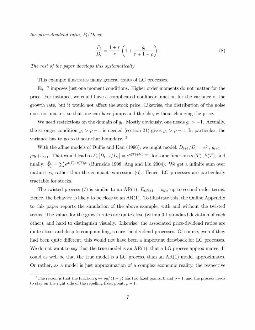
the price-dividend ratio, Pt/Dt is:

Pt

Dt=1 + r

r

µ1 +

gtr + 1− ρ

¶. (8)

The rest of the paper develops this systematically.

This example illustrates many general traits of LG processes.

Eq. 7 imposes just one moment conditions. Higher order moments do not matter for the

price. For instance, we could have a complicated nonlinear function for the variance of the

growth rate, but it would not affect the stock price. Likewise, the distribution of the noise

does not matter, so that one can have jumps and the like, without changing the price.

We need restrictions on the domain of gt. Mostly obviously, one needs gt > −1. Actually,the stronger condition gt > ρ− 1 is needed (section 21) gives gt > ρ− 1. In particular, thevariance has to go to 0 near that boundary. 3

With the affine models of Duffie and Kan (1996), we might model: Dt+1/Dt = egt , gt+1 =

ρgt+εt+1. That would lead toEt [Dt+T/Dt] = ea(T )+b(T )gt, for some functions a (T ) , b (T ), and

finally: PtDt=P

ea(T )+b(T )gt (Burnside 1998, Ang and Liu 2004). We get a infinite sum over

maturities, rather than the compact expression (6). Hence, LG processes are particularly

tractable for stocks.

The twisted process (7) is similar to an AR(1), Etgt+1 = ρgt, up to second order terms.

Hence, the behavior is likely to be close to an AR(1). To illustrate this, the Online Appendix

to this paper reports the simulation of the above example, with and without the twisted

terms. The values for the growth rates are quite close (within 0.1 standard deviation of each

other), and hard to distinguish visually. Likewise, the associated price-dividend ratios are

quite close, and despite compounding, so are the dividend processes. Of course, even if they

had been quite different, this would not have been a important drawback for LG processes.

We do not want to say that the true model is an AR(1), that a LG process approximates. It

could as well be that the true model is a LG process, than an AR(1) model approximates.

Or rather, as a model is just approximation of a complex economic reality, the respective

3The reason is that the function g 7→ ρg/ (1 + g) has two fixed points, 0 and ρ− 1, and the process needsto stay on the right side of the repelling fixed point, ρ− 1.

7

advantage of LG vs affine models depends on the specific task at hand. The modeler should

be able to pick whichever modelling approximation is most expedient, and LG processes offer

one such choice.

We now start our systematic treatment of LG processes. As several factors are needed

to capture the dynamics of stocks (Campbell and Shiller 1988, Fama and French 1996) and

bonds (Litterman and Scheinkman 1991), we study the multifactor case.

3 Linearity-generating processes in discrete time

This section studies the discrete-time LG processes. We want to price an asset with dividend

Dt, given a discount factorMt.4 The price at time t of a claim yielding a stochastic dividend

Dt+T at maturity T ≥ 0 is: Pt = E

" ∞XT=0

Mt+TDt+T

#/Mt. For instance, the price at t of a

(“zero coupon”) bond yielding 1 in T periods is: Zt (T ) = Et [Mt+T ] /Mt.

3.1 Definition and main properties

The state vector is Xt ∈ Rn (n ∈ N∗) and can be generally thought of as stationary, whileMtDt generally trends, and is not stationary. The definition of the LG process is the follow-

ing.

Definition 1 The processMtDt (1, X0t)t=0,1,2,..., withMtDt ∈ R∗ and Xt ∈ Rn, is a linearity-

generating process if there are constants α ∈ R, γ, δ ∈ Rn,Γ ∈ Rn×n, such that the following

relations hold at all t ∈ N:

Et

∙Mt+1Dt+1

MtDt

¸= α+ δ0Xt (9)

Et

∙Mt+1Dt+1

MtDtXt+1

¸= γ + ΓXt (10)

4The simplest example is Mt = (1 + r)−t. If a consumer with utility

Pt δ

tU (Ct) prices assets, thenMt = δtU 0 (Ct). Also, some authors call “stochastic discount factor” Mt+1/Mt. In this context, there is noconfusion.

8

To interpret (9), consider first the case of bonds, Dt ≡ 1. Eq. 9 says that the properly-defined interest is linear in the factors. WhenMt = (1 + r)−t, (9) says that expected dividend

growth is linear in the factors. In general, (9) means that the expected value of the (dividend

augmented) stochastic discount factor growth is linear in the factors.

Condition (10) mean that, Xt follows “twisted” AR(1). It behaves in some sense like

Et [Xt+1] = γ + ΓXt, but it is twisted by theMt+1Dt+1

MtDtterm. Another useful interpretation

of (10) is that it specifies the factor dynamics under the risk-neutral measure induced by

MtDt.

What kinds of models are compatible with Definition 1? As the examples below show,

it is not difficult to write toy economic models satisfying conditions (9)-(10), e.g. in Lucas

(1978) and Campbell-Cochrane (1999) economies with exogenous consumption, dividend or

marginal utility processes, or models with learning. Farhi and Gabaix (2007) and Gabaix

(2007) presents a fully worked-out economic model satisfying the conditions of Definition 1.

Indeed, conditions (9)-(10) give a prescription to “reverse-engineer” macro or micro fun-

damentals, so as to make the model tractable: The modeler has to make sure that the

endowment, technology etc. is such that (9)-(10) hold.

In addition, models that to not directly fit into the conditions of Definition 1, could be

approximated by projected linearly in (9)-(10). Also, by extending the state vector, equations

(9)-(10) could hold to an arbitrary degree of precision. The Online Appendix to this paper

illustrates how to approximate a non-LG process with an LG process, even to an arbitrary

degree of precision.

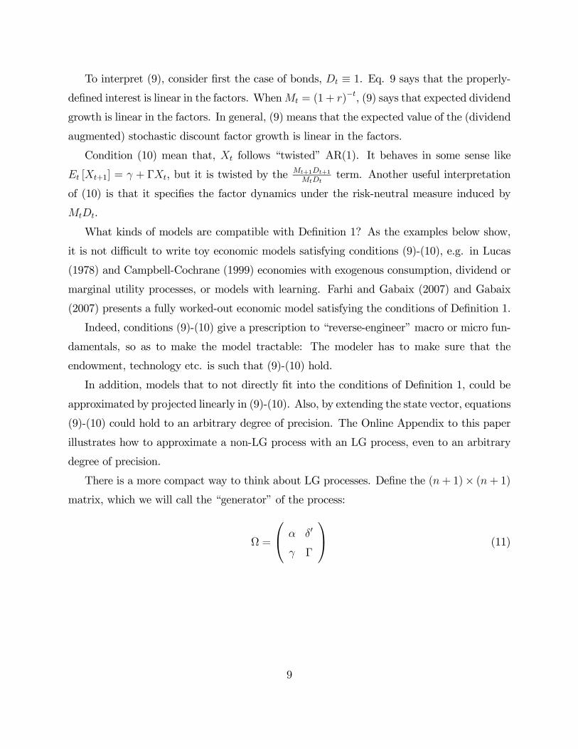
There is a more compact way to think about LG processes. Define the (n+ 1)× (n+ 1)matrix, which we will call the “generator” of the process:

Ω =

⎛⎝ α δ0

γ Γ

⎞⎠ (11)

9

and the process with values in Rn+1

Yt :=

⎛⎝ MtDt

MtDtXt

⎞⎠ =

⎛⎜⎜⎜⎜⎜⎝MtDt

MtDtX1t

...

MtDtXnt

⎞⎟⎟⎟⎟⎟⎠ , (12)

so that with vector ν 0 = (1, 0, ..., 0),

Mt = ν 0Yt (13)

Yt stacks all the information relevant to the prices of the claims derived below. 5 Conditions

(9)-(10) can be written:

Et [Yt+1] = ΩYt. (14)

Hence, the (dividend-augmented) stochastic discount factor of a LG process is simply the

projection (Eq. 13) of an autoregressive process, Yt. The tractability of LG processes comes

from the tractability of autoregressive processes.

The basic pricing properties are the following two Theorems.

Theorem 1 (Bond prices, discrete time) The price-dividend ratio of a zero-coupon equity

or bond of maturity T , Zt (T ) = Et [Mt+TDt+T ] / (MtDt), is

Zt (T ) =³1 0n

´·

⎛⎝ α δ0

γ Γ

⎞⎠T

·

⎛⎝ 1

Xt

⎞⎠ (15)

= αT + δ0αT In − ΓT

αIn − ΓXt when γ = 0 (16)

where In the identity matrix of dimension n, and 0n is the row vector with n zeros.

For instance, when Dt ≡ 1, the above Theorem can price bonds, with n factors, in closedform.

In many applications (e.g., the examples in this paper), γ = 0, which means the state

variables are re-centered around 0. For instance, the state variable is the deviation of the

5Other assets, e.g. options, require of course to know more moments.

10

equity premium from its trend value.

The second main result is the most useful property of LG processes: the existence of a

closed-form formula for stock prices.

Theorem 2 (Stock prices, discrete time) Suppose that all eigenvalues of Ω have a modulus

less than 1 (finiteness of the price). Then, the price-dividend ratio of the stock, Pt/Dt =

Et [P∞

s=tMsDs] / (MtDt), is:

Pt/Dt =1

1− α− δ0 (In − Γ)−1 γ

¡1 + δ0 (In − Γ)−1Xt

¢(17)

=³1 0n

´·

⎛⎝In+1 −

⎛⎝ α δ0

γ Γ

⎞⎠⎞⎠−1 ·⎛⎝ 1

Xt

⎞⎠ . (18)

Theorem 2 allows to generate stock prices with an arbitrary number of factors, including

time-varying growth rate, and risk premia.

Tomake formulas concrete, consider the case where Γ is a diagonal matrix: Γ ≡ Diag (Γ1, ...,Γn),

i.e.

Ω =

⎛⎜⎜⎜⎜⎜⎝α δ1 · · · δn

γ1 Γ1 0 0... 0

. . . 0

γn 0 0 Γn

⎞⎟⎟⎟⎟⎟⎠ .

Then, αT In+1−ΓTαIn+1−Γ = Diag

¡¡αT − ΓTi

¢/ (α− Γi)

¢,6 so that (16) and (17) read:

Zt (T ) = αT +nXi=1

αT − ΓTiα− Γi

δiXit if γ = 0 (19)

Pt/Dt =1 +

Pni=1

δiXi

1−Γi

1− α−Pn

i=1δiγi1−Γi

(20)

Finally, the following Propositions show that one can price claims that have dividend a linear

function of DtXt. In bond applications, they show that futures price obtain in closed form.

6If A matrix, and f : R → R, is analytic with f (x) =P∞

n=0 fnxn then f (A) =

P∞n=0 fnA

n. IfA = Diag (a1, .., an), f (A) = Diag (f (a1) , ..., f (an))

11

The proofs are exactly identical to those of the previous two Theorems.

Proposition 1 (Value of a single-maturity claim yielding Dt+T δ0Xt+T ). Given the LG

process MtDt (1,Xt), the price of a claim yielding a dividend dt = Dt

nXi=1

fiXit = Dt (f0Xt),

Pt = Et [Mt+Tdt+T ] /Mt, is:

Pt =

⎛⎝0f

⎞⎠0⎛⎝ α δ0

γ Γ

⎞⎠T ⎛⎝ 1

Xt

⎞⎠Dt (21)

= f 0ΓTXtDt when γ = 0. (22)

Proposition 2 (Value of an asset yielding Dtδ0Xt at each period) Under the conditions

of Theorem 2, the price of a claim yielding a dividend dt = Dt

nXi=1

fiXit = Dtf0Xt, Pt =

Et [P∞

s=tMsDs] /Mt is,

Pt =

⎛⎝0f

⎞⎠0⎛⎝In+1 −

⎛⎝ α δ0

γ Γ

⎞⎠⎞⎠−1⎛⎝ 1

Xt

⎞⎠Dt =f 0 (In − Γ)−1 (γ + (1− α)Xt)

1− a− δ0 (In − Γ)−1 γDt. (23)

For instance, when Γ ≡ Diag (Γ1, ...,Γn), Eq. 22 and 23 read:

Pt/Dt =nXi=1

fiΓTi XitDt if γ = 0

Pt/Dt =

nXi=1

fi1−Γi (γi + (1− α)Xit)

1− α−Pn

i=1δiγi1−Γi

3.2 Some examples

We now work out some examples. The derivations are in Appendix B.

Example 2 A Gordon growth formula with time-varying dividend growth.

12

In this example, we generalize our introductory stock example. Suppose that the interest

rate is constant at r, dividend Dt, and the growth rate of dividend is:

Dt+1

Dt= (1 + g∗) (1 + xt)

¡1 + ηt+1

¢xt+1 =

ρxt1 + xt

+ εt+1 (24)

where ηt is some unimportant i.i.d. noise, greater than -1, independent of the innovation to

εt+1. xt is the deviation from the trend growth rate. If xt was an AR(1), it would follow

Et [xt+1] = ρxt. Instead, the process is slightly modified, to (24), to make the process LG.

Indeed, with Mt = (1 + r)−t, and using the notation 1 +R = (1 + r) / (1 + g∗), we calculate

the two LG moments:

Et

∙Mt+1Dt+1

MtDt

¸= (1 + xt) / (1 +R)

Et

∙Mt+1Dt+1

MtDtxt+1

¸= Et

∙Mt+1Dt+1

MtDt

¸Et [xt+1] =

(1 + xt)

1 +R

ρxt1 + xt

=ρxt1 +R

In the above equation, the 1 + xt terms cancel out, because of the 1 + xt term in the

denominator of (24). We designed the process so that the LG equation (10) holds.

So MtDt (1, xt) is LG, with Ω =

⎛⎝ 1/ (1 +R) 1/ (1 +R)

0 ρ/ (1 +R)

⎞⎠ =

⎛⎝ α δ0

γ Γ

⎞⎠. Hence, weapply Theorem 2, with a dimension n = 1, γ = 0, α = 1/ (1 +R), δ = Γ = αρ. We obtain,

for the price-dividend ratio, Pt/Dt =1

1−α−δ0(In−Γ)−1γ

¡1 + δ0 (In − Γ)−1Xt

¢, i.e.

Pt/Dt =1 +R

R

µ1 +

1

1 +R− ρxt

¶(25)

Hence we see how Example 1 comes from the general structure of LG processes.

Example 3 Stock price with stochastic growth rate and stochastic equity premium

13

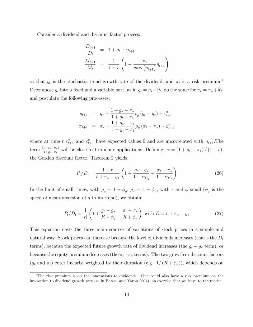
Consider a dividend and discount factor process:

Dt+1

Dt= 1 + gt + ηt+1

Mt+1

Mt=

1

1 + r

Ã1− πt

vart¡ηt+1

¢ηt+1!

so that gt is the stochastic trend growth rate of the dividend, and πt is a risk premium.7

Decompose gt into a fixed and a variable part, as in gt = g∗+bgt, do the same for πt = π∗+bπt,and postulate the following processes:

gt+1 = g∗ +1 + g∗ − π∗1 + gt − πt

ρg (gt − g∗) + εgt+1

πt+1 = π∗ +1 + g∗ − π∗1 + gt − πt

ρπ (πt − π∗) + επt+1

where at time t εgt+1 and επt+1 have expected values 0 and are uncorrelated with ηt+1.The

term (1+g∗−π∗)1+gt−πt will be close to 1 in many applications. Defining: α = (1 + g∗ − π∗) / (1 + r),

the Gordon discount factor. Theorem 2 yields:

Pt/Dt =1 + r

r + π∗ − g∗

µ1 +

gt − g∗1− αρg

+πt − π∗1− αρπ

¶(26)

In the limit of small times, with ρg = 1 − φg, ρπ = 1 − φπ, with r and φ small (φg is the

speed of mean-reversion of g to its trend), we obtain:

Pt/Dt =1

R

µ1 +

gt − g∗R+ φg

− πt − π∗R+ φπ

¶with R ≡ r + π∗ − g∗ (27)

This equation nests the three main sources of variations of stock prices in a simple and

natural way. Stock prices can increase because the level of dividends increases (that’s the Dt

terms), because the expected future growth rate of dividend increases (the gt − g∗ term), or

because the equity premium decreases (the πt−π∗ terms). The two growth or discount factors(gt and πt) enter linearly, weighted by their duration (e.g., 1/ (R+ φπ)), which depends on

7The risk premium is on the innovations to dividends. One could also have a risk premium on theinnovation to dividend growth rate (as in Bansal and Yaron 2004), an exercise that we leave to the reader.

14

the speed of mean-reversion of the each process (parametrized by φπ, φg), and the effective

discount rate, R. The volatility terms do not enter in (27), and the price does not change if

one changes the correlation between the instantaneous innovation in gt and πt.

Example 4 A multifactor bond model with bond risk premia (in discrete time).

There are n factors rit. The stochastic discount factor is:

Mt+1

Mt=

1

1 + r∗

Ã1−

nXj=1

rjt

!(28)

The short term rate is rt = 1/Et

hMt+1

Mt

i− 1 ' r∗ +

Prit if the r’s are small. Each factor rit

is postulated to evolve as:

ri,t+1 =ρiri,t

1−P

rjt+ ηi,t+1 (29)

where Etηi,t+1 = 0, but the ηi,t+1 can otherwise have any correlation structure. This is a LG

process. The bond price is:

Zt (T ) =1

(1 + r∗)T

Ã1−

nXi=1

1− ρTi1− ρi

rit

!(30)

This expression is quite simple, and accommodates a wide variety of specifications for

the factors, Eq. 29. Furthermore, it accommodates bonds with risk premia. Just take

a stochastic discount factor: Mt+1

Mt= 1

1+r∗

³1−

Pnj=1 rjt

´+ εt+1, where Etεt+1 = 0, but

otherwise εt+1 is unspecified, and can be heteroskedastic. and postulate: ri,t+1 =ρiri,t

1− rjt+

ηi,t+1 −Et[εt+1·ηi,t+1]Et[Mt+1/Mt]

, which means that rit follow the process (29) under the risk-neutral

measure. Then, Eq. 30 holds. The risk premium on the T maturity bond is:

Risk premium =cov (εt+1, Zt+1 (T − 1))

Zt (T )=(1 + r∗)

P 1−ρT−1i

1−ρicov

¡εt+1, ηi,t+1

¢1−

P 1−ρTi1−ρi

rit

Hence we easily generate an explicit yield curve. With a parametrization for cov¡εt+1, ηi,t+1

¢,

the above expression makes predictions for bond risk premia across maturities (see Gabaix

2007).

15

Example 5 Markov chains, and some economies with learning

There are n states. In state i the factor-augmented dividend grows at a rateGi: Mt+1Dt+1/ (MtDt) =

Gi. Call Xit ∈ 0, 1, equal to 1 if the state is i, 0 otherwise. The probability of going fromstate j to state i is called pij. Then, MtDt (1, X1, ..., Xn) is a LG process. Hence, a Markov

chain belongs to the LG class.8 As many processes are (arbitrarily) well-approximated by

discrete Markov chains, they are (arbitrarily) well-approximated by LG processes.

Markov chains induced by learning naturally lead to LG processes. For a complete

example, the reader is encouraged to read Veronesi (2005). He finds that if Xit is the agents’

probability estimate that the economy is in state i, under canonical models with Gaussian

filtration of information, then vector Xt follows an autoregressive process. He works out

the prices of stocks and bonds in an economy, and finds that they are linear function of Xt.

Hence, some canonical structural with learning models naturally give rise to LG processes.

Example 6 Flexible LG parametrization of state variables the stochastic discount factor

Take an n−dimensional process Xt, such that:

Mt+1Dt+1

MtDt= a+ β0Xt + εt+1

Xt+1 =γ + ΓXt

a+ β0Xt

+ ηt+1 −Et

£εt+1ηt+1

¤a+ β0Xt

(31)

with Et [εt+1] = 0, Et

£ηt+1

¤= 0. Then, Eq. 9-10 are satisfied. Section 5 provides conditions

to ensure MtDt > 0 for all times.

To interpret (31), consider the case γ = Et

£εt+1ηt+1

¤= 0. Eq. 31 expresses that, when

Xt is small, Et [Xt+1] =ΓXt

a+β0Xt∼ Γ

axt, which means that Xt follows approximately at AR(1).

The corrective 1 + β0/a ·Xt in the denominator is often small in practice, but ensures that

the process is LG.

In many applications, there is no risk premium on the factor risk, so that Et

£εt+1ηt+1

¤=

0. However, when there is a risk-premium equation (31) means that it is enough to know

that the process under the “risk-neutral” measure.

8Veronesi and Yared (2000) and David and Veronesi (2006) have already seen that this type of Markovchain yielded prices that are linear in the factors.

16

We next turn to the continuous time version of what we have seen so far.

4 Linearity-generating processes in continuous time

We fix a probability space¡ΩP ,F , P

¢and an information filtration Ft satisfying the usual

technical conditions (see, for example, Karatzas and Shreve 1991). The stochastic discount

factor is Mt. For applications, we will express the results in terms of a dividend-augmented

stochastic discount factor, MtDt. Often, it is better to imagine Dt ≡ 1.

4.1 Definition and main properties

A notation. The following notation is useful when using LG processes. For xt, μt processes

in a vector space V , we say Et [dxt] = μtdt, or Et [dxt] /dt = μt, to signify that there exists

a martingale Nt with values in V such that: xt = x0 +R t0μsds+Nt.

The definition in continuous time is analogous to the definition in discrete time. The

vector of factors is Xt.

Definition 2 The process MtDt (1,Xt)0t∈R+, with MtDt ∈ R and Xt ∈ Rn, is a linearity-

generating process if there are constants with a ∈ R, b, β ∈ Rn,Φ ∈ Rn×n, such that the

following relations hold at all t ∈ R+,

Et [d (MtDt)] = − (a+ β0Xt)MtDtdt (32)

Et [d (MtDtXt)] = − (b+ ΦXt)MtDtdt (33)

The interpretation is exactly the same as for Definition 1. Eq. 32 means that the expected

growth rate of MtDt is linear in the factors. Eq. 33 means that Xt follows a twisted AR(1).

Loosely speaking, it describes the process for Xt under the “risk-neutral” measure induced

by MtDt.

For instance, in the case Dt ≡ 1 and dMt/Mt = − (a+ β0Xt) dt, Eq. 33 gives:

dXt = −bdt− (Φ− aIn)Xtdt+ (β0Xt)Xtdt+ dNt (34)

17

whereNt ∈ Rn is a martingale. Hence, the process contains an AR(1) term,−b−(Φ− aIn)Xt,

plus a “twist” quadratic term, (β0Xt)Xt. It is a “twisted” AR(1). In many applications, Xt

represents a small deviation from trend, and the quadratic term (β0Xt)Xt is small. We are

agnostic about how empirically relevant the “twist” is. It could be that it is absent in the

physical probability, but present under the risk-neutral measure.

So Et [dNt] = 0, but its components dNit, dNjt can be correlated. The simplest type of

martingale is dNt = σ (Xt) dBt, for Bt a Brownian motion, but richer structures, e.g. with

jumps, are allowed. As in the one-factor process, the volatility of dNt must go to zero in

some limit regions for the process to be well-defined. We defer this more technical issue until

section 5.

As in the discrete-time case, we define the “generator” of the process:

ω =

⎛⎝ α β

b Φ

⎞⎠ (35)

and the process Yt =

⎛⎝ MtDt

MtDtXt

⎞⎠ ∈ Rn+1, as in (12), which encodes the information

needed for prices. Conditions (32)-(33) write more compactly as:

Et [dYt] = −ωYtdt. (36)

which is the analogue of (14). The above process leads to a LG discrete-time process with

time increments ∆t, with a generator Ω = e−ω∆t.

Hence, there is a (n+ 1) dimensional process Yt, and a vector ν 0 = (1, 0, ..., 0), such

that (36) holds, and Mt = ν 0Yt. In other terms, there is a autoregressive process Yt in

the background, following (36). The (dividend-augmented) stochastic discount factor is the

one-dimensional projection of it. LG processes are tractable, because they are the one-

dimensional projection of an AR(1) process.

The next Theorem prices claims of finite maturity.

Theorem 3 (Bond prices, continuous time). The price-dividend of a claim on a dividend

18

of maturity T , Zt (T ) = Et [Mt+TDt+T ] / (MtDt), is:

Zt (T ) =³1 0n

´· exp

⎡⎣−⎛⎝ a β0

b Φ

⎞⎠T

⎤⎦ ·⎛⎝ 1

Xt

⎞⎠ (37)

= e−aT + β0e−ΦT − e−aT In

Φ− aInXt when b = 0 (38)

where In the identity matrix of dimension n, and 0n is the row vector with n zeros.

As an example, bond prices come from Dt = 1. In many applications, b = 0, which can

generically be obtained by re-centering the variables.

Theorem 4 is probably the most useful of this section.

Theorem 4 (Stock prices, continuous time). Suppose that all eigenvalues of ω have pos-

itive real part (finite stock price). Then, the price/dividend ratio of the stock, Pt/Dt =

Et

£R∞t

MsDsds¤/ (MtDt) , is:

Pt/Dt =1− β0Φ−1Xt

a− β0Φ−1b(39)

=³1 0n

´·

⎛⎝ a β0

b Φ

⎞⎠−1 ·⎛⎝ 1

Xt

⎞⎠ (40)

To make things more concrete, consider the case where Φ is a diagonal matrix: Φ =

Diag (Φ1, ...,Φn), i.e.:

ω =

⎛⎜⎜⎜⎜⎜⎝a β1 · · · βn

b1 Φ1 0 0... 0

. . . 0

bn 0 0 Φn

⎞⎟⎟⎟⎟⎟⎠ (41)

Then, e−ΦT = Diag¡e−ΦiT

¢, and then (16) and (17) read:

Zt (T ) = e−at +nXi=1

e−ΦiT − e−aT

Φi − aβiXit if b = 0 (42)

Pt/Dt =1−

Pni=1

βiXit

Φi

a−Pn

i=1βibiΦi

(43)

19

Finally, the following Propositions show that one can price claims that have dividend

a linear function of DtXt. The proofs are exactly identical to those of the previous two

Theorems.

Proposition 3 (Value of a single-maturity claim yielding Dt+Tf0Xt+T ). Given the LG

process MtDt (1,Xt), the price of a claim yielding a dividend dt = Dt

nXi=1

fiXit = Dt (f0Xt),

Pt = Et [Mt+Tdt+T ] /Mt, is:

Pt =

⎛⎝0f

⎞⎠0

· exp

⎡⎣−⎛⎝ a β0

b Φ

⎞⎠T

⎤⎦ ·⎛⎝ 1

Xt

⎞⎠Dt (44)

= f 0e−ΦTDtXt when b = 0. (45)

Proposition 4 (Value of an asset yielding Dtf0Xt at each period) Under the conditions

of Theorem 4, the price of a claim yielding a dividend dt = Dt

nXi=1

fiXit = Dtf0Xt, Pt =

Et

£R∞t

Msdsds¤/Mt, is,

Pt =

⎛⎝0f

⎞⎠0

ω−1

⎛⎝ 1

Xt

⎞⎠Dt =f 0Φ−1 (−b+ aXt)

a− β0Φ−1bDt. (46)

4.2 Some examples

We start with some stock-like examples.

Example 7 Simple stock example with LG stochastic trend growth rate, in continuous time

We study Example 1 in continuous time. Suppose MT = e−rT , DT = D0 exp³R T

0gtdt

´,

with the continuous time limit of (5):

dgt =¡−φgt − g2t

¢dt+ σ (gt) dzt (47)

20

In the equation above, the coefficient on g2t has to be −1. Theorem 4 yields:9

Pt/Dt =1

r

µ1 +

gtr + φ

¶. (48)

Section 5 will present the condition gt ≥ −φ for the process to be well defined. We nextgeneralize the example to n factors.

Example 8 Dividend growth rate as a sum of mean-reverting processes (e.g., a slow and a

fast process).

We extend the previous example to a several factors. Suppose MT = e−rT , DT =

D0 exp³R T

0gtdt

´, with gt = g∗ +

Pni=1Xit and

Et [dXit] /dt = −φiXit + (g∗ − gt)Xitdt.

The growth rate gt is a steady state value g∗, plus the sum of mean-reverting processes Xit.

EachXit mean-reverts with speed φi, and also has the quadratic perturbation (g∗ − gt)Xitdt.

The price-dividend ratio is

Pt/Dt =1

r − g∗

Ã1 +

nXi=1

Xit

r − g∗ + φi

!. (49)

Each component Xit perturbs the baseline Gordon expression 1/ (r − g∗). The perturbation

isXit, times the duration ofXi, discounted at rate r−g∗, which is the term 1/ (r − g∗ + φi).10

9The result in Example 7 appear new to the literature. The Fisher-Wright process does contain a quadraticterm, but it has not been applied to the pricing bonds or stocks. Also, it is more special than the LG class,because it imposes a specific functional form on the variance. Cochrane, Longstaff, and Santa-Clara (forth.)apply the Fisher-Wright process. Mele (2003, forth.) identifies a condition for the process to be linear in thefactor, but does not derive stocks and bond prices such as (48). Other papers introduce different quadraticterms in stochastic process, for instance Ahn et al. (2002), and Constantidines (1992) but they do not takethe form of this paper.10The formula suggests the following non-LG variant. Suppose we have a process with dψt =

(rtψt + αrt − β) dt+dNt,where dNt is an adapted martingale, and is essentially arbitrary except for technicalconditions. Then Vt = (ψt + α) /β is a solution of the perpetuity arbitrage equation: 1−rtVt+E [dVt] /dt = 0.If the process well-defined for t ≥ 0, then Vt is the price of a perpetuity, Vt = Et

hR∞t

e−strududs

i.

For instance, with the process d (1/rt) = φ (rt − r∗) dt + dNt, the price of a perpetuity is: Vt =(1/rt + φ/r∗) / (1 + φ).

21

Terms that mean-revert more slowly have a higher impact on the the price. Finally, Theorem

3 yields:

Et [Dt+T ] = eg∗T

Ã1 +

nXi=1

1− e−φiT

φiXit

!Dt.

Example 9 Generalized Gordon formula, with stochastic trend in dividend growth, and sto-

chastic equity premium, in continuous time.

We present the continuous time version of Example 3. The stochastic discount factorMt

and the dividend process Dt follow

dMt/Mt = −rdt−πtσdzt and dDt/Dt = gtdt+ σdzt

The price of the stock is Pt = Et

£R∞t

MsDsds¤/Mt. πt is a the stochastic equity premium,

and gt is the stochastic growth rate of dividends.

We assume that πt and gt follow the following LG process, best expressed in terms of

their deviation from trend, bπt = πt − π∗,bgt = gt − g∗:

dbgt = −φgbgtdt+ (bπt − bgt)bgtdt+ σγ (bgt, bπt) · dBt

dbπt = −φπbπtdt+ (bπt − bgt) bπtdt+ σπ (bgt, bπt) · dWt

where the (Bt,Wt) is a Wiener process independent of zt, that can have arbitrary time- or

state-dependent correlations, and σγ and σπ are vector-valued processes. We suppose that

the process is defined in [t,∞). Again the processes dbgt and dbπt are to a first order linear,but with quadratic “twist” terms added, (bπt − bgt) bgtdt and (bπt − bgt) bπtdt. The stock price is

Pt =Dt

R

µ1 +

gt − g∗R+ φg

− πt − π∗R+ φπ

¶with R ≡ r + π∗ − g∗ (50)

where R is the traditional Gordon rate.11 As in Example 3, this example nests the three

sources of variation in prices, movements in dividends (Dt), in expected growth rate of

dividends (gt), and of discount factor (πt).

11It is a good and simple exercise to derive the above formula directly, from the arbitrage equation1− (r + πt − gt) (P/D)t +E [d (P/D)t] /dt = 0.

22

Example 10 The aggregate model of Menzly, Santos and Veronesi (2004), and the Bhat-

tacharya (1978) mean-reverting process, belong to the linearity-generating class.

The following point is simple and formal. Menzly, Santos and Veronesi (MSV, 2004)

rely on an Ornstein-Uhlenbeck. The inverse of their consumption-surplus ratio, yt, follows:

Et [dyt] = k (y − yt) dt. The price-consumption ratio in their economy is Vt = y−1t Et

£R∞0

e−ρsyt+sds¤.

In terms of the LG process, the state variable is yt, andMt = e−ρt. We haveEt [dMt/dt] /Mt =

−ρdt, and Et [d (Mtyt) /dt] /Mt = −ρyt+k (y − yt). SoMt (1, yt) is a LG process with gener-

ator ω =

⎛⎝ ρ 0

−kY ρ+ k

⎞⎠. The MSV pricing equation 17 comes directly from Proposition4 of the present article, ytVt = (ky + ρyt) / [ρ (ρ+ k)]. Hence, in retrospect, the MSV (2004)

process is tractable because it belongs to the LG class. This remark, also, immediately

suggest a way to formulate the MSV paper to discrete time. In a simpler context, Bhat-

tacharya (1978) models the dividend yt as an Ornstein-Uhlenbeck, yielding the same closed

form solution for the price.

Example 11 A LG process where the stock price is convex (not linear) in the growth rate

of dividends

This “academic” example shows how one can obtain asset prices that are increasing in

their variance, which is important in some applications (Johnson 2002, Pastor and Veronesi

2003). Consider an economy with constant discount rate r (i.e. Mt = e−rt), and a stock with

dividend Dt = D0 exp³R t

0gsds

´, where12 dgt = − (g2t /2 + φgt) dt+

pk (G2 − g2)dzt. Then,

the price-dividend ratio is:

Pt/Dt =2(φ+ r)(2φ+ k + r) + 2(2φ+ k + r)gt + g2t

2r (φ+ r) (2φ+ k + r)− kG2(51)

which is increasing in the parameter G of the volatility. In this example, the state vector

is (gt, g2t ), which makes the price quadratic and convex in gt. More generally, by expanding

the state vector, the price could be a polynomial of arbitrary order in g.

We next present some bond-like examples. We start with a very simple example.

12We assume 0 < G < 2 (φ− k), and that the support of gt is (−G,G), with end points natural boundaries.

23

Example 12 A one-factor bond model, with an always positive nominal rate.

The following example is simply illustrates LG processes. It has just one factor, whereas

multifactor models are necessary to capture the yield curve. SupposeMt = exp³−R t0rsds

´,

with rt = r∗ + brt, withdbrt = − (φ− brt) brtdt+ dNt

where φ > 0, brt ≤ φ, and Nt is a martingale, which could include a diffusive part and a jump

part. The bond price is:

Zt (T ) = e−r∗Tµ1 +

e−φT − 1φ

brt¶ . (52)

The independence of bond prices from volatility greatly simplifies the analysis. In par-

ticular, dNt could have jumps, which model a decision by the central bank, or fat-tailed

innovations of other kinds (Gabaix et al. 2006). One does not need to specify the volatility

process to obtain the prices of bonds: only the drift part is necessary. This leaves a high

margin of flexibility to calibrate volatility, for instance on interest rate derivatives, a topic

we do not pursue here.

How can we ensure that the interest rate always remains positive? That is very easy

(with r∗ > 0). For instance, we could have dNt = σ (rt) dzt, where zt is a Brownian process,

with σ (r) ∼ k0rκ0, κ0 > 1/2 for r in a right neighborhood of 0, and k0 > 0, so that the

local drift at rt = 0 is positive. By the usual Feller conditions on natural boundaries, the

process admits a strong solution, and rt ≥ 0 always (Cheridito and Gabaix 2007 spell outthe technical conditions). And, the bond price (52) is not changed by this assumption about

the volatility process. One can indeed change the lower bound for the process (if it is less

than r∗) without changing the bond price.

Section 5 will detail the conditions for the existence of the process. The interest rate

needs to remains below some upper bound r ∈ (r∗, r∗ + φ], so as to not explode. One way is

to assume that σ (r) ∼ k (r − r)κ, for r in a left neighborhood of r, κ > 1/2 and k > 0. Given

the drift is negative around r, that will ensure that r is a natural boundary, and ∀t, rt ≤ ralmost surely, as detailed in Cheridito and Gabaix (2007). We next turn to the canonical

LG bond case.

Example 13 A multifactor bond model, with bond risk premia (continuous time).

24

The following is Example 4 in continuous time. Suppose dMt/Mt = −rtdt+ dNt, where

Nt is a martingale, and decompose the short rate in rt = r∗ +Pn

i=1 rit, with r∗ a constant

and:

Et [drit] + hdrit, dMt/Mti = [−φirit + (rt − r∗) rit] dt (53)

where we use the notation hdxt, dyti is the usual bracket, e.g. hσ1 · dBt, σ2 · dBti = σ1 · σ2dt.

Hence, it is enough to specify the process “under the risk-neutral measure”. One does not

need to separately specify the dynamics of Et [drit] and its risk premium, the hdrit, dMt/Mtiterm. Only the sum matters. The process Mt (1, r1t, ..., rnt) is LG13, and the bond price is

Zt (T ) = e−r∗T

Ã1−

nXi=1

1− e−φiT

φirit

!. (54)

The risk-premium at t on the T−maturity zero coupon, π (T ) := −DdZt(T )Zt

, dMt

Mt

E/dt can

be simply expressed too.

Example 14 Lucas economy where stocks, bonds, and a continuum of moments can be

calculated.

We consider a Lucas economy with: dCtCt= gtdt+dN

Ct , var

¡dNC

t

¢= σ2dt, dgt = −φgtdt+

dNgt ,Ddgt,

dCtCt

E= −gt (gt −A) dt, with A > 0, and Ng

t , NCt are martingales, and gt ≤ A.

Then:

∀α ≤ 0,∀T ≥ 0, Et

£Cαt+T

¤= Cα

t eα(α−1)σ2

2t

µ1 +

1− e−(φ−αA)T

(φ− αA)αgt

¶(55)

The eα(α−1)σ2

2t term is the expected Jensen’s inequality term. The novel term is the gt term.

This way, if the agent has utilityRe−ρtC1−γ

t / (1− γ) dt, one can calculate all the bonds

prices in a Lucas economy, and the price of a claim on consumption.

13The generator is ω =

⎛⎜⎜⎜⎝r∗ 1 · · · 10 r + φ1 0 0

0 0. . . 0

0 0 0 r + φn

⎞⎟⎟⎟⎠.

25

5 Conditions to keep the process well-defined

The results of this paper require that the process be defined for t ≥ 0, and in particular

that MtDt > 0, which ensures the above-derived prices are positive. This section provide

simple sufficient conditions to ensure that. They are meant to be practical and easy to verify.

Cheridito and Gabaix (2007) provide more abstract and general conditions.

5.1 Discrete time

We start with Example 1. We want the process to be well-defined. Write gt+1 =ρgt+σ(gt)ηt+1

1+gt,

with Et

£ηt+1

¤= 0 and σ (gt) ≥ 0. First, take the case where there is no noise, ∀t, ηt+1 = 0.

The application g 7→ ρg/ (1 + g) has two fixed points, an attractive one g = 0, and a repelling

one that, g = ρ− 1. To ensure that the process is economically meaningful, we require thatg0 be on the right side of the repelling point, g0 > ρ− 1. That will ensure (when there is nonoise) that for all t ≥ 0, gt > ρ− 1, and in particular gt > −1. If g0 < ρ− 1, then for sometime t, gt < −1, not a meaningful economic outcome. In conclusion, in the deterministicgrowth rate case, we want to impose

gt > g = ρ− 1. (56)

When the growth rate is stochastic, we want that for all gt+1 > ρ−1, i.e. gt+σ (gt) ηt+1 >g. This is possible if ηt+1 has a lower bound, and the volatility σ (g) goes to 0 fast enough

near the boundary g, a fact formalized in the next Lemma.

Lemma 1 (Conditions of existence of the process in the 1-dimensional, discrete time case).

Consider the process in Example 1: gt+1 =gt+σ(gt)ηt+1

1+gt, with Et

£ηt+1

¤= 0. Assume that (i)

there is an m > 0 such that, almost surely, for all t, ηt+1 > −m ; and (ii) 0 ≤ σ (g) ≤ g−gm,

i.e. the volatility goes to 0 fast enough close to g = ρ − 1. Suppose g0 > g. Then, almost

surely, for all t ≥ 0, gt > g, and the process is defined for all times t.

The principle generalizes to several factors. Consider the discrete-time case where the

26

generator Ω is of the form (??), with α > 0 and α > Γi for all i, and γ = 0.14 Parametrize

the noise in (14) by Yt+1 = ΩYt + Yt0ut+1, where Et [ut+1] = 0. The n−factor generalizationof the criterion (56) above is the following:

Proposition 5 (Condition to ensure a well-behaved process, with positive stochastic discount

factor, discrete time) Suppose that M0D0 > 0, and that at t = 0, X0 satisfies:

Condition C at time t (discrete time): 1 +nXi=1

min (δiXit/α, 0)

1− Γi/α> 0 (57)

Suppose also that the noise ut+1 is bounded and goes to 0 fast enough near the boundary of

(57). Then, for all times t ≥ 0, MtDt > 0, so that the process is well-defined, and prices

Et [Mt+TDt+T ] are positive. In addition, for all times t, Xt satisfies the condition (57).

The first part of the Proposition implies that, if the noise is small enough, then all prices

derived above will be positive. The second part, means that if Condition C is satisfied at

t = 0, then it will be satisfied for all future t’s. This “self-perpetuating” property makes it

potentially useful for applied work.

Condition C means δiXit terms should not be too negative. It means that growth rates

terms should not be too low, and interest rate terms should not be too high. This makes

sense, because, in view of (19), if the terms δiXit are too negative, then prices could be

threaten to be negative.

To illustrate this, consider first Example 2. Then, δ = 1, α = 1/ (1 +R), Γ1 = ρα, and

the condition reads: 1+min (xt, 0) / (1− ρ) > 0, i.e. xt > 1−ρ. This is exactly the condition(56) derived above. The deviation of the growth rate from trend cannot be too low.

Next, consider Example 4. Then, α = 1/ (1 + r∗), δ = α (−1, ...,−1), and Γ = α (ρ1, ..., ρn).

Condition C reads: 1 +Pn

i=1min(−rit,0)

1−ρi> 0, i.e.

1−nXi=1

max (rit, 0)

1− ρi> 0. (58)

14This case is not very restrictive, as more general case can be reduced to it by diagonalization, if Ω isdiagonalizable in R.

27

This condition means that the components of the interest rate state vector cannot be too

positive. Each component is weighted by its duration 1/ (1− ρi), i.e. more persistent com-

ponents count for more.

Finally, consider the hybrid Example 3. The condition reads: 1+min (gt − g∗, 0) /¡1− ρg

¢−

max (πt − π∗, 0) / (1− ρπ) > 0. This means that the growth rate should not be too low, or

the risk premium should not be too high.

5.2 Continuous time

The same condition carries over to continuous time. In the case where ω is equal to (41)

with b = 0, and a < Φi for all i, the condition is:

Condition C at time t (continuous time): 1−nXi=1

max (βiXit/a, 0)

Φi − a> 0 (59)

For instance, for the simple growth model of Example 7, we have Xt = gt, a = r, β = −1,Φ = φ+ r, so Condition C gives: 1−max (−gt, 0) /φ > 0, i.e. gt > −φ, the continuous timelimit of (56).

Likewise, for the interest rate model of Example 12, the condition is brt < φ. The interest

rate should not be too high.

In the multi-factor model of Example 13, a = r∗, β = 1,Φi = r∗ + φi, so the Condition

is: 1−Pn

i=1max (rit, 0) /φi > 0, which is just the continuous time analogue of (58).

This conclude our simple, practical sufficient conditions for processes to be well-defined.

More abstract and general conditions are provided in Cheridito and Gabaix (2007).

6 Extensions

This section presents additional results and remarks on LG processes.

28

6.1 LG processes are the only ones that generate linearity

We show that, in a certain sense, if bond prices are linear in the factors, then they come

from an LG process. To see that, let us first consider the 1-factor case. Call Xt the factor,

and suppose that for T = 1, 2, Zt (T ) = αT + βTXt, for some numbers α1, β1 6= 0, α2, β2.With T = 1, we get Et [Mt+1/Mt] = α1 + β1xt, so that condition (9) holds. Also,

α2 + β2Xt = Et

∙Mt+2

Mt

¸= Et

∙Mt+1

MtEt+1

∙Mt+2

Mt+1

¸¸= Et

∙Mt+1

Mt(α1 + β1Xt+1)

¸= α1 (α1 + β1Xt) + β1Et

∙Mt+1

MtXt+1

¸

Et

∙Mt+1

MtXt+1

¸=1

β1(α2 + β2Xt − α1 (α1 + β1Xt)) = a00 + b00Xt

hence (10) holds. We conclude that if both the 1 and 2-period maturity bonds are affine in

Xt, then Mt (1,Xt) is a LG process. The next Proposition shows that the property holds

with n factors15

Proposition 6 (LG processes are the only processes generating linear bond prices) Sup-

pose that there are coefficients for some coefficients (αT , βT , )T≥0, with (αT , βT ) , T = 1, 2..spanning Rn+1

. , such that ∀t, T ≥ 0, Et [Mt+T/Mt] = αT + β0TXt, Then, Mt (1,Xt) is a LG

process, i.e. there is a matrix Ω, such that Yt =Mt (1,Xt)0 follows: Et [Yt+1] = ΩYt.

6.2 Relation to the affine-yield class

The affine class (Duffie and Kan 1996; Dai and Singleton 2000; Duffie, Pan and Singleton

2000; Duffee 2002; Cheridito, Filipovic and Kimmel 2007) is a very important class, that

contains the processes of Vasicek and Cox, Ingersoll, Ross (1985). It is a workhorse of

much empirical and theoretical in asset pricing. It comprises processes of the type: dXt =

15The property that (αT , βT ) , T = 1, 2.. spans Rn+1. means that Et [Mt+T /Mt] = αT + β0TXt is themost compact representation of the process. More precisely, if it didn’t span Rn+1. , one could find a striclylower dimensional process xt ∈ Rm. , m < n, and constants AT , BT , such that Et [Mt+T /Mt] = AT + B0

Txt.Indeed, call γT =

¡αT , β

0T

¢0, and V = Span γT , T ≥ 0. If V is a strict subset of Rn+1. , decompose

Rn+1. = V ⊕ V ⊥, call B : V → Rn+1. the natural injection, and h·, ·i the restriction of the Euclidean producton V . Then, γ0 (T )Yt = (Bγ (T ))

0Yt = γ (T )

0B0Yt, so we have Zt (T ) = γ (T )

0(B0Yt). Vector B0Yt has

dimension dimV < n+ 1.

29

(b− ΦXt) dt + wtdzt, with wtw0t = σ2 (H 0

1Xt +H0), with b,Xt ∈ Rn, Φ ∈ Rn×n, (H0, H1) ∈Rn×n × Rn×n×n, σ ∈ R, zt is a n−dimensional Brownian motion. The interest rate is rt =r∗ + β0 (Xt −X∗), where X∗ = Φ−1b, is assumed to exist. Under mild technical conditions,

bond prices have the expression:

ZAfft (T ) = exp¡−r∗T + Γ (T )0 (Xt −X∗) + σ2a (T )

¢,

where a (T ) and Γ (T ) satisfy coupled ordinary differential equations, that typically need

to be solved numerically. This is not a problem for empirical work, but that does hinder

theoretical work. The situation is simpler if H1 = 0. In that case, Γ (T ) = γ (T ), with

γ (T )0 = β0¡e−ΦT − 1

¢/Φ. Then: ZAfft (T ) = exp

¡−r∗T + γ (T )0 (Xt −X∗) + σ2a (T )

¢. This

expression can be contrasted with the expression for the LG process (38),

ZLGt (T ) = e−r∗T¡1 + γ (T )0 (Xt −X∗)

¢. (60)

If γ (T )0Xt is small, the two expressions are the same, up to terms of second order in γ (T )0Xt,

and second order in σ. Hence, a LG process is a good approximation if the underlying process

is in fact affine, and vice-versa. In most cases, the two values are likely to be close, so that

existing estimates of parameters in the affine class can be used to calibrate LG processes.16

What are the respective merits of the LG and affine classes? First, quantitatively, they

will often make close predictions, as the two models yield the same prices to a first or-

der. Hence, for many situations, the choice of affine vs LG processes is just a matter of

convenience.

In terms of the economic differences, as LG bond prices are independent of volatility

(controlling for the covariances, see Eq. 54), LG processes generate “unspanned volatility,”

a relevant feature of the data, as shown by Collin-Dufresne and Goldstein (2002), Andersen

and Benzoni (2007) and Joslin (2007). By contrast, affine models typically impose a tight

16That equivalence gives a useful way to calculate easily functionals of LG processes, that can be expressedas a linear combination of bonds. One first works with the affine process, setting volatility to 0, doing afirst order Taylor expansion of terms in (Xt −X∗). One gets an expression: PAfft = a + b (Xt −X∗) +o (Xt −X∗) + o

¡σ2¢, for some constant a, b. Then, one knows that for the corresponding LG process, the

value of the asset is: P LGt = a+ b (Xt −X∗), exactly.

30

link between bond prices and volatility.

On the other hand, a potential drawback of pricing bonds with the LG process, is that,

in the simplest version at least, bonds have no mechanically-induced convexity in the LG

framework. However, this may not be such a problem, as Joslin (2007) estimates that bond

convexity plays a small role in bond prices. In addition, multifactor LG processes can have

some convexity (Example 11).

Coming now to the difference in terms of tractability, the distinctive advantage of the

LG class is for stocks. LG yield simple closed forms for stock prices. However, with the

affine class, a stock price can be only be expressed PAfft /Dt =

P∞t=0 Z

Afft (T ) (Burnside 1998,

Ang and Liu 2004). Those are infinite sums of exponentials, which is a great progress over

stochastic sums, but are still not very tractable.

Beyond their advantage for stocks, LG processes have two lesser virtues. First, bond

prices are quite simple, which should prove useful to theorize on bonds (Gabaix 2007).

Second, LG processes allow a free functional form for the innovations dNt, which can include

jumps and non-Gaussian behavior, and a free type of heteroskedascity.

On the other hand, affine processes are the central technique to price derivatives, whereas

this paper is silent about options (pricing options with LG processes is an open challenge).

Finally, affine models are now well-understood, and they have been estimated. It would be

very desirable to do the same for LG models (see Binsbergen and Koijen 2007)

In conclusion, LG processes have a good advantage for stocks, and affine processes have

a strong advantage for options. For bonds, affine models will continue to be tremendously

useful, but LG models may complement them, particularly in theoretical research.

6.3 Processes with time-dependent coefficients

It is simple to extend the process to time-dependent deterministic coefficients, i.e. in Defin-

ition 1, to have α, δ, γ,Γ functions of time. With Yt = (Mt,MtXt)>, this is Et [Yt+1] = ΩtYt,

where Ωt =

⎛⎝ αt δ0t

γt Γt

⎞⎠. That implies E0 [YT ] = T−1Yt=0

ΩtY0. Hence, in the zero-coupon

expressions, it is enough to replace ΩT byT−1Yt=0

Ωt.

31

6.4 Closedness under addition and multiplication

The product of two uncorrelated LG processes is LG. The product of two un-

correlated LG processes with respective dimensions d1, d2 (i.e., with d1− 1 and d2− 1 factorrespectively) is LG, with dimension d1d2 (i.e., with d1d2 − 1 factors). The idea is simple,though it requires somewhat heavy notations.

We start in discrete time. Take two LG processes characterized by M it , Y

it ,Ω

i, and con-

sider a process with discount factorMt =M1t M

2t . Assume that, for any index i, j of the com-

ponents, cov³Y1(i)t+1 , Y

2(j)t+1

´= 0. The innovations between processes are uncorrelated, but,

importantly, not necessarily independent. Then, it is easy to verify that for any vector ψi,

Et

£¡ψ1Y 1

T

¢ ¡ψ2Y 2

T

¢¤= Et

£ψ2Y 2

T

¤Et

£ψ2Y 2

T

¤. In particular, Et [M

1TM

2T ] = Et [M

1T ]Et [M

2T ].

Then,Mt =M1t M

2t is also the stochastic discount factor of a LG process. The underlying

autoregressive process is Y1

t ⊗ Y2

t , i.e. the vector made of the d1d2 components Y1(i)

t Y2(j)

t ,

i = 1...d1, j = 1...d2. The corresponding generator Ω is Ω = Ω1 ⊗ Ω2.

The same reasoning holds in continuous time. Starting with processes M it , Y

it , ω

i, and

assumingDdY

1(i)t+1 , dY

1(2)t+1

E= 0, then M1

t M2t is also a pricing kernel that comes from a LG

process. The underlying autoregressive process is Y1

t ⊗ Y2

t (which has dimension d1d2), and

it is easy to check that the generator is: ω = ω1⊗Id2+Id1⊗ω2. To make the above concrete,consider the following example.

Example 15 Stock with decoupled LG processes for the growth rate and the risk premium.

Consider processes with dMt/Mt = −rt − λtdBt, dDt/Dt = gtdt + σtdBt, where gt

follows: dgt = −φg (gt − g∗) dt − (gt − g∗)2 dt + dNg

t , and the risk premium, πt = λtσt,

follows: dπt = −φπ (πt − π∗) dt+(πt − π∗)2 dt+dNπ

t , whereNgt , N

πt are martingales. Assume

that the processes dNgt , dN

πt and dBt are uncorrelated. Then, the price of a stock, Pt =

E0£R∞0

MtDtdt¤/M0, is Pt/Dt = Et

£R∞s=texp

¡−R su=t(r + πu − gu) du

¢ds¤. In virtue of the

above properties,

Et

∙exp

µZ s

t

−πu + gudu

¶¸= Et

∙exp

µZ s

t

−πudu¶¸

Et

∙exp

µZ s

t

gudu

¶¸.

For general processes, the above equation would in general require the two processes to

be independent — for instance, with stochastic volatility, the respective variance processes

32

should be independent. For LG processes, the property required is the weaker hdπt, dgti = 0for all t’s.

Using the values of the LG processes, and integrating, we obtain, with R = r+π∗− g∗,17

Pt/Dt =1

R

"1− πt − π∗

R+ φπ+

gt − g∗R+ φg

−¡2R+ φπ + φg

¢(πt − π∗) (gt − g∗)

(R+ φπ)¡R+ φg

¢ ¡R+ φπ + φg

¢ # . (61)

The central value is again the Gordon formula, Pt/Dt = 1/R. It is modified by the current

level of the equity premium, and the growth rate of the stock. A stock with a currently high

growth rate gt exhibits a higher price-dividend ratio, and this is amplified when the equity

premium is low, as shown by the term (πt − π∗) (gt − g∗).

The difference between formula (61) and formula (50) is that in (61), the processes for πt

and gt are decoupled, whereas in (50), they were coupled, i.e. in their drift term there was a

term (gt − g∗). The decoupling forces the presence of a cross term (πt − π∗) (gt − g∗) in the

expression of the price. In general, one obtains simpler expressions by having one multifactor

LG processes, rather than the product of many different LG processes. With n coupled

factors, the stock price has n+ 1 terms, while with n decoupled factors, the stock price has

2n terms.

The sum of two LG processes is LG. This property is quite trivial, and mentioned

for completeness. Suppose two LG process M it , Y

it ,Ω

i, with M it = νiY i

t , for i = 1, 2. Call di

the dimension of Y it . Then, Mt =M1

t +M2t comes from a LG process of dimension d1 + d2.

Indeed, define Yt = (Y 1t , Y

2t ), ν = (ν

1, ν2), and Ω =

⎛⎝ Ω1 0

0 Ω2

⎞⎠. Then, Et [Yt+1] = ΩYt,

and Mt = ν 0Yt.

7 Conclusion

Linearity-generating processes are very tractable, as they yield closed forms for stocks and

bonds, and prices that are linear in factors. They are likely to be useful in several parts of

17Menzly, Santos and Veronesi (2004, Eq. 20) obtain a similar expression. This is natural because the LGclass embeds their model, as Example 10 shows.

33

economics, when trend growth rates, or risk premia, are time-varying. The results of this

paper suggest the following research directions.

Most importantly, LG processes allow the construction of paper and pencil tractable

general equilibrium models, with closed forms for stocks and bonds. Indeed they suggest a

way to “reverse engineer” the processes for endowments and technology, so that the model

is tractable. Gabaix (2007) and Farhi and Gabaix (2007) present such models.

Second, it would be good to use the flexibility and closed forms of LG processes for

empirical work. In an ambitious new paper, Binsbergen and Koijen (2007) take up this task,

and demonstrate the fruitfulness of having closed forms for multifactor models. Also, since

the LG processes are defined by moment conditions (Eq. 9-10), they lend themselves to

estimation and testing by GMM techniques.

Third, LG processes suggest a new way to linearize models. Given a model, one could do a

Taylor expansion expressing moments Et [Mt+1Dt+1/MtDt] and Et [Mt+1Dt+1Xt+1/MtDt] as

a linear function of the factors, thereby making Eq. 9-10 hold to a first order approximation.

The projected model is then in the LG class, and its asset prices are approximations of the

prices of the initial problem. Hence the LG class offers a way to derive linear approximations

of the asset prices of more complicated models. The Online Appendix to this paper studies

such an example, where a non-LG process can be approximated by an LG process to an

arbitrary degree of precision.

Fourth, LG processes can be enriched by a decision variable, and offer a way to do

multifactor, closed-form dynamic programming. I explore those issues in ongoing research.

I conclude that LG processes might be a useful addition to the economist’s toolbox.

Appendix A. Matrix Algebra

Derivations with LG processes often use the following Lemmas, which are standard.

Lemma 2 With a ∈ R, b, c ∈ Rn, and d ∈ Rn×n, suppose that d is invertible and that the

real number a − b0d−1c is 6= 0. Then the (n+ 1) × (n+ 1) matrix

⎛⎝ a b0

c d

⎞⎠ is invertible,

34

and its inverse is: ⎛⎝ a b0

c d

⎞⎠−1 = 1

a− b0d−1c

⎛⎝ 1 −b0d−1

−d−1c ad−1

⎞⎠ (62)

Lemma 3 With n ∈ N∗+, a ∈ R, b ∈ Rn, and d ∈ Rn×n. Call 0n the n−dimensional vectormade of 0’s, In the n−dimensional identity matrix, and suppose that aIn − d is invertible.

Then, for T ∈ N∗,

⎛⎝ a b0

0n d

⎞⎠T

=

⎛⎝ aT b0¡aT In − dT

¢(aIn − d)−1

0n dT

⎞⎠and, for T ∈ R,

exp

⎡⎣⎛⎝ a b0

0n d

⎞⎠T

⎤⎦ =⎛⎝ eaT b0

¡eaT In − edT

¢(aIn − d)−1

0n edT

⎞⎠Appendix B. Additional Derivations

7.1 Derivation of Theorems and Propositions

Proof of Theorem 1 Recall (14), Et [Yt+1] = ΩYt. Iterating on T , it implies that for

all T ≥ 0, Et [Yt+T ] = ΩTYt. Given Mt+T = ν 0Yt+T ,

Zt (T ) = (MtDt)−1Et [Mt+TDt+T ] = (MtDt)

−1Et [ν0Yt+T ] = (MtDt)

−1 ν 0Et [Yt+T ]

= (MtDt)−1 ν 0ΩTYt = ν 0ΩT

¡(MtDt)

−1 Yt¢= ν0ΩT

⎛⎝ 1

Xt

⎞⎠ =³1 0n

´ΩT

⎛⎝ 1

Xt

⎞⎠i.e. (15). The formula for γ = 0 comes from Lemma 3 in Appendix A.

35

Proof of Theorem 2 We use (15), which gives the perpetuity price:

Pt/Dt =∞XT=0

Zt (T ) = ν 0

à ∞XT=0

ΩT

!⎛⎝ 1

Xt

⎞⎠ = ν 0 (In+1 − Ω)−1

⎛⎝ 1

Xt

⎞⎠P∞

T=0ΩT is summable because all eigenvalues of Ω have a modulus less than 1. We use

Lemma 2 from Appendix A to calculate (In − Ω)−1, and conclude.18

Proof of Theorem 3 Recall the definition of ω in (35), and Et [d (Yt)] = −ωYtdt. Itis well-known that this implies19: ∀T ≥ 0, Et [Yt+T ] = e−ωTYt. Given Mt+T = ν 0Yt+T ,

Zt (T ) = (MtDt)−1Et [Mt+TDt+T ] = (MtDt)

−1Et [ν0Yt+T ] = (MtDt)

−1 ν 0Et [Yt+T ]

= (MtDt)−1 ν 0e−ωTYt = ν 0e−ωT

¡(MtDt)

−1 Yt¢= ν 0e−ωT

⎛⎝ 1

Xt

⎞⎠ =³1 0n

´e−ωT

⎛⎝ 1

Xt

⎞⎠ .

i.e. Eq. 37. The formula for b = 0 comes from Lemma 3 in Appendix A.

Proof of Theorem 4 We use (37). The perpetuity price is:

Pt/Dt =

Z ∞

0

Zt (T ) dT = ν 0µZ ∞

0

e−ωTdT

¶·

⎛⎝ 1

Xt

⎞⎠ = ν 0ω−1 ·

⎛⎝ 1

Xt

⎞⎠We use the Lemma 2 to calculate ω−1, and conclude.20

18There is a more elementary heuristic proof. We seek a solution of the type Pt/Dt ≡ Vt = c− 1 + h0Xt,

which we know exists, by summation of (15). The arbitrage equation is: Vt = 1 +EhMt+1Dt+1

MtDtVt+1

i, i.e.

c+h0Xt = 1+E

∙Mt+1Dt+1

MtDt(c+ h0Xt)

¸= 1+ c

¡α+ δ0Xt

¢+h0 (γ + ΓYt) = [1 + cα+ h0γ] +

£cδ0 + h0Γ

¤Xt

i.e. (i) c = 1 + cα + h0γ and (ii) h0 = cδ0 + h0Γ. (ii) gives h0 = cδ0 (1− Γ)−1, and plugging in (i) yieldsch1− α− δ0 (1− Γ)−1 γ

i= 1, hence c and (17).

19In the case t = 0 (which is enough), the proof is thus: define f (T ) = E0 [YT ]. Then, df (T ) = E0 [dYT ] =E0 [−ωYTdT ] = −ωE0 [YT ] dT = −ωf (T ) dT , which integrates to f (T ) = e−ωT f (0), i.e. E0 [YT ] = e−ωTY0.20The following elementary heuristic proof is useful to know. We seek a solution of the type Pt/Dt ≡ Vt =

c+h0Xt, which we know exists, by integration of (37). The arbitrage equation is: 1− rtVt+E [dVt] /dt = 0,

36

Proof of Proposition 5 Write Yt = (Y0t, ..., Ynt), with Y0t = MtDt, and define Ht =

Y0t +Pn

i=1min(δiYit,0)

α−Γi . Start with the case of where there is no noise, i.e. ∀t, Yt+1 = ΩYt.

Given Ω, this means Y0,t+1 = αY0t +P

i δiYit, and for i ≥ 1, Yi,t+1 = ΓiYi,t. So:

Ht+1 = αY0t +Xi

δiYit +Xi

min (δiΓiYit, 0)

α− Γi

= αY0t +X

i s.t. δiYit>0

δiYit +X

i s.t. δiYit≤0

µ1 +

Γiα− Γi

¶δiYit

≥ αY0t +X

i s.t. δiYit≤0

α

α− ΓiδiYit = αHt.

Hence, Ht+1 ≥ αHt. Hence, if H0 > 0, then ∀t ≥ 0, Ht > 0, and so that MtDt = Y0t ≥Ht > 0.

In the case with noise, say that Yt+1 = ΩYt + ut+1, for some mean 0 noise ut+1, and

suppose that ut+1 is bounded. By continuity, if Ht > 0, Ht+1 is positive with probability 1,

if ut+1 is small enough. And again, MtDt = Y0t ≥ Ht > 0.

Proof of Proposition 6 Call Yt = Mt (1,Xt)0, γT = (αT , βT )

0, so that Et [Mt+T ] =

γ0TYt. That implies γ0T+1Yt = Et [Mt+T+1] = Et [Et+1 [Mt+T+1]] = Et [γTYt+1], hence: γ

0T+1Yt =

Et [γTYt+1].

Call ek ∈ Rn+1. , the vector with k−th coordinate equal to 1, and other coordinates equal

to 0. AsγT , T = 1, 2, .. spans Rn+1. , there are reals λkT (with at most n+1 non-zero values)

such that: ek =P

T λkTγT . Define Ω =P

k,T ekλkTγ0T+1. Given In+1 =

n+1Xk=1

eke0k, we have:

Et [Yt+1] =

ÃXk

eke0k

!Et [Yt+1] =

ÃXk

ek

ÃXT

λkTγ0T

!!Et [Yt+1]

=Xk,T

ekλkTEt [γ0TYt+1] =

Xk,T

ekλkTγ0T+1Yt = ΩYt.

i.e.1−

¡r∗ + β0Xt

¢(c+ h0Xt) + h0

£b− ΦXt +

¡β0Xt

¢Xt

¤= 0

This holds if and only if the constant and the term inXt are zero, i.e. r∗h0+β0c+h0Φ = 0 and 1−r∗c+h0b = 0.

Hence h0 = −β0c (r∗ + Φ)−1 and 1− cr∗+β0 (r∗ + Φ)−1

b = 0, which gives c = 1/hr∗ + β0 (r∗ + Φ)

−1bi, and

yields (39).

37

7.2 Derivations of Examples

Example 3 Define bπt = πt − π∗,bgt = gt − g∗, so that:

Et

∙Mt+1

Mt

Dt+1

Dt

¸=

1

1 + r(1 + gt − πt) = α+

bgt − bπt1 + r

Et

∙Mt+1

Mt

Dt+1

Dtbgt+1¸ = Et

∙Mt+1

Mt

Dt+1

Dt

¸Et [bgt+1] = 1

1 + r(1 + gt − πt)·

1 + g∗ − π∗1 + gt − πt

ρgbgt = αρgbgtThe analogue expression holds for bπt. Hence The process Yt = MtDt (1, bπt,bgt)0 is LG, withgenerator

⎛⎜⎜⎝α 1/ (1 + r) −1/ (1 + r)

0 αρg 0

0 0 αρπ

⎞⎟⎟⎠. Applying (17) yields the result.

Example 4 We have Et

hMt+1

Mtri,t+1

i= 1

1+r∗ρiri,t. So process Mt (1, r1,t, ..., rn,t) has

generator: 11+r∗

⎛⎜⎜⎜⎜⎜⎝1 −1 · · · −10 ρ1 0 0

0 0. . . 0

0 0 0 ρn

⎞⎟⎟⎟⎟⎟⎠. By (11) and (16), the bond price obtains.

Example 5 Et

hMt+1Dt+1

MtDt

i=P

iGiXit, and

Et

∙Mt+1Dt+1

MtDtXi,t+1

¸= Et

∙Mt+1Dt+1

MtDt

¸Et [Xi,t+1] =

ÃXk

GkXkt

!ÃXj

pijXjt

!=Xj

pijGjXjt

as XktXjt = 0 if j 6= k, and otherwise is equal to XktXjt = Xjt, as exactly one of the Xjt is

6= 0.

Example 7 Et [d (MtDt) / (MtDt)] = (−r + gt) dt and

Etd (Mtgt) = gt·Et [dMt]+MtEtdgt = gt·(−r + gt)Mtdt+Mt

¡−φgt − g2t

¢dt = − (r + φ) gtMtdt

38

We note that the g2t terms cancel out, which is their raison d’etre in (47). So Mt (1, gt) is a

LG process with generator ω =

⎛⎝r −10 r + φ

⎞⎠.Example 8 We calculate the LG moments:

Et

∙d (MtDt)

MtDt

¸/dt = − (r − g∗) +

nXi=1

Xjt

Et

∙d (MtDtXit)

MtDt

¸/dt =

"− (r − g∗) +

nXi=1

Xjt

#Xit +

Ã−φiXit −

ÃnXi=1

Xit

!Xit

!= − (r − g∗ + φi)Xit,

soMtDt (1,X1t, ...,Xnt) is a LG process, with generator: ω =

⎛⎜⎜⎜⎜⎜⎝r − g∗ −1 · · · −10 r − g∗+φ1 0 0

0 0. . . 0

0 0 0 r − g∗+φn

⎞⎟⎟⎟⎟⎟⎠.We apply the Theorem 3, with a = r−g∗, β0 = (−1, ...,−1), Φ = Diag (r − g∗ + φ1, ..., r − g∗ + φn).

Example 9 We calculate the LG moments:

Et

∙d (MtDt)

MtDt

¸/dt = −r − πt + gt = −R− bπt + bgt

Et

∙d (MtDtbgt)

MtDt

¸/dt = Et

∙d (MtDt) /dt

MtDt

¸ bgt +Et [bgt] /dt= (−R− bπt + bgt) bgt +− ¡φg − bπt + bgt¢ bgt = − ¡R+ φg

¢ bgtand likewise for Et

hd(MtDtπt)

MtDt

i/dt = − (R+ φπ) bπt. So MtDt (1,bg, bπt) is LG with generator⎛⎜⎜⎝

R 1 1

0 R+ φg 0

0 0 R+ φπ

⎞⎟⎟⎠.

39

Example 11 Calculation shows that Yt = e−rT (Dt,Dtg,Dtg2t ) is a LG process, with

generator ω =

⎛⎜⎜⎝r −1 0

0 r + φ −1/2−kG2 −b r + k + 2φ

⎞⎟⎟⎠.Example 12 We calculate the LG moments: dMt/Mt = −rtdt = − (r∗ + brt) dt, and:

d (Mtbrt)Mt

= brtdMt

Mt+ dXt = −brt (r∗ + brt) dt+− (φ− brt) brtdt+ σtdNt

= − (r∗ + φ) brtdt+ σtdNt

Importantly, the br2t terms cancel out. So, using Et [dNt] = 0, we have the LG moments:

Et [dMt/Mt] /dt = −r∗ − brt and Et [d (Mtbrt) /Mt] /dt = − (r∗ + φ) brtSo Yt =Mt (1, brt) is LG with generator

⎛⎝r∗ 1

0 r∗ + φ

⎞⎠.Example 14 Et

dCαt

Cαt= αgt + α (α− 1) σ2

2and

Et [d (Cαt gt)]

Cαt dt

=

µαgt + α (α− 1) σ

2

2

¶gt − φgt + α

¿dgt,

dCt

Ct

À=

µαgt + α (α− 1) σ

2

2

¶gt − φgt − αgt (gt −A) =

µ−φ+ αA+ α (α− 1) σ

2

2

¶gtdt

so, Cαt (1, gt) is a LG process with generator ω =

⎛⎝α (α− 1) σ22

α

0 α (α− 1) σ22− φ+ αA

⎞⎠.The statement follows. The process is well-defined if α (gt −A) > −φ, which is ensured ifthe volatility of gt goes to 0 fast enough at gt = A, so that always gt ≤ A.

References

Ahn, Dong-Hyun, Robert F. Dittmar, and A. Ronald Gallant (2002), “Quadratic Term Structure

Models: Theory and Evidence,” Review of Financial Studies, 15, 243-288.

40

Andersen, Torben G. and Luca Benzoni (2007), “Do Bonds Span Volatility Risk in the U.S.

Treasury Market? A Specification Test for Affine Term Structure Models,” NBER WP 12962.

Ang, Andrew and Jun Liu (2004), “How to Discount Cashflows with Time-Varying Expected

Returns,” Journal of Finance, 59, 6, 2745-2783.

Bakshi, Gurdip S. and Zhiwu Chen (1997), “An Alternative Valuation Model for Contingent

Claims,” Journal of Financial Economics, Vol 44, No. 1, 1997, 123-165.

Bansal, Ravi and Amir Yaron (2004), “Risks for the Long Run: A Potential Resolution of Asset

Pricing Puzzles,” Journal of Finance, 59, 1481-1509.

Barro, Robert (2006), “Rare Disasters and Asset Markets in the Twentieth Century,” Quarterly

Journal of Economics, 121, 823-866.

Bhattacharya, S. (1978), “Project Valuation with Mean Reverting Cash Flow Streams,”Journal

of Finance, 33, 1317—31.

Binsbergen, Jules H. van and Ralph S.J. Koijen (2007), “Predictive Regressions: A Present-

Value Approach,” Working Paper, Duke University.

Boudoukh, Jacob, Matthew Richardson and Robert Whitelaw (forth.): “The Myth of Long-

Horizon Predictability,” Review of Financial Studies.

Burnside, Craig (1998), “Solving Asset Pricing Models with Gaussian Shocks,” Journal of

Economic Dynamics and Control, 22, 329-40.

Campbell, John Y., and John Cochrane (1999), “By Force of Habit: A Consumption-Based

Explanation of Aggregate Stock Market Behavior,” Journal of Political Economy, 107, 205-251.

Campbell, John Y., and Robert J. Shiller (1988), “The Dividend-Price Ratio and Expectations

of Future Dividends and Discount Factors,” Review of Financial Studies, 1, 195-228.

Campbell, John Y. and Shiller, Robert J. (1991), “Yield Spreads and Interest Rate Movements:

A Bird’s Eye View,” Review of Economic Studies, 58, 495—514.

Cheridito, Patrick, Damir Filipovic and Robert L. Kimmel (2007), “Market Price of Risk Spec-

ifications for Affine Models: Theory and Evidence,” Journal of Financial Economics, 83, 123-170.

Cheridito, Patrick, and Xavier Gabaix (2007), “Regularity Conditions to Ensure the Existence

of Linearity-Generating Processes” Working Paper, New York University.

Cochrane, John (forth.), “The Dog That Did Not Bark: A Defense of Return Predictability,”

Review of Financial Studies.

41

Cochrane, John, Francis Longstaff, Pedro Santa-Clara (forth.), “Two Trees,” Review of Finan-

cial Studies.

Collin-Dufresne, Pierre, and R. S. Goldstein (2002), “Do Bonds Span the Fixed IncomeMarkets?

Theory and Evidence for Unspanned Stochastic Volatility,” Journal of Finance, 57, 1685-1730.

Constantinides, George M. (1992) “A Theory of the Nominal Term Structure of Interest Rates,”

Review of Financial Studies, 5, 531-552

Cox, John C., J. E. Ingersoll, Jr., and Stephen A. Ross (1985), “A Theory of the Term Structure

of Interest Rates,” Econometrica, 53, 385-407.

Croce, M., Martin Lettau, and Sydney Ludvigson (2006), “Investor Information, Long-Run

Risk, and the Duration of Risky Cash Flows,” Mimeo, New York University.

Dai, Qiang and Kenneth J Singleton (2000), “Specification Analysis of Affine Term Structure

Models,” The Journal of Finance, 55(5), 1943—1978.

David, Alexander, and Pietro Veronesi (2006), “Inflation and Earnings Uncertainty and Volatil-

ity Forecasts,” Working Paper, University of Chicago.

Duffee, G. (2002), “Term Premia and Interest Rate Forecasts in Affine Models,” Journal of

Finance, 57, 405—43.

Duffie, D., and R. Kan (1996), “A Yield-Factor Model of Interest Rates,”Mathematical Finance,

6, 379-406.

Duffie, D., J. Pan, and K. Singleton (2000), “Transform Analysis and Asset Pricing for Affine

Jump Diffusions,” Econometrica, 68, 1343-1376.

Fama, E., and K. R. French (1996), “Multifactor Explanations of Asset Pricing Anomalies,”

The Journal of Finance, 51, 55-84.

Farhi, Emmanuel and Xavier Gabaix (2007), “Rare Disasters and Exchange Rates: A Theory

of the Forward Premium Puzzle,” Working Paper, Harvard University and NYU.

Gabaix, Xavier (2007), “A Simple, Unified, Exactly Solved Framework for Ten Puzzles in

Macro-Finance,” Working Paper, NYU.

Gabaix, Xavier, and David Laibson (2002), “The 6D Bias and the Equity Premium Puzzle,”

NBER Macroeconomics Annual, 16, 257-312.

Gabaix, X., P. Gopikrishnan, V. Plerou, and H. E. Stanley (2006), “Institutional Investors and

Stock Market Volatility,” Quarterly Journal of Economics, 121, 461—504.

42

Hansen, Lars, John C. Heaton, and N. Li (2005), “Consumption Strikes Back? Measuring Long

Run Risk,” NBER WP 11476.

Hansen, Lars, and José Scheinkman (2006), “Long Term Risk: An Operator Approach,” Mimeo,

Princeton University.

Johnson, Timothy C. (2002), “Rational Momentum Effects,” The Journal of Finance, 57 (2),

585-608.

Joslin, Scott (2007), “Pricing and Hedging Volatility Risk in Fixed Income Markets,” Working

Paper, MIT.

Julliard, Christian, and Jonathan Parker (2005), “Consumption Risk and the Cross-Section of

Expected Returns,”Journal of Political Economy, 113, 185-222.

Lettau, Martin and Jessica Wachter (2007), “Why is Long-Horizon Equity Less Risky? A

Duration-Based Explanation of the Value Premium,”Journal of Finance.

Litterman, R., and José Scheinkman (1991), “Common Factors Affecting Bond Returns,” Jour-

nal of Fixed Income, 1, 54-61.

Liu, Jun (2007), “Portfolio Selection in Stochastic Environments,” Review of Financial Studies,

20, 1-39.

Mamaysky, Harry (2002), “A Model For Pricing Stocks and Bonds,” Yale ICF Working Paper

No. 02-10.

Mele, Antonio (2003), “Fundamental Properties of Bond Prices in Models of the Short-Term

Rate,” Review of Financial Studies, 16, 679-716.

Mele, Antonio (forth.), “Asymmetric Stock-Market Volatility and the Cyclical Behavior of

Expected Returns,” Journal of Financial Economics.

Menzly, Lior, Tano Santos, and Pietro Veronesi (2004), “Understanding Predictability,” Journal

of Political Economy, 112, 1-47.

Pastor, Lubos, and Pietro Veronesi (2003), “Stock Valuation and Learning about Profitability,”

Journal of Finance, 58, 1749-1789.

Pastor, Lubos, and Pietro Veronesi (2005), “Rational IPO Waves,” Journal of Finance, 60,

1713 — 1757.

Ross, Stephen A. (1978), “A Simple Approach to the Valuation of Risky Streams”, The Journal

of Business, 51,453-475.

43

Santos, T., and P. Veronesi (2006), “Labor Income and Predictable Stock Returns,” Review of

Financial Studies, 19, 1-44.

Sims, Christopher A. (1990), “Solving the Stochastic Growth Model by Backsolving with a

Particular Nonlinear Form for the Decision Rule,” Journal of Business & Economic Statistics, 8,

45-47

Vasicek, Oldrich (1977): “An equilibrium characterization of the term structure,” Journal of

Financial Economics, 5, 177-188

Veronesi, Pietro (2005), “Teaching Notes on Asset Pricing,” Chapter 3.

Veronesi, Pietro, and Pierre Yared (2000), “Short and Long Horizon Term and Inflation Risk

Premia in the US Term Structure,” mimeo, University of Chicago.

44

Online Appendix for “Linearity-Generating Processes: AModelling Tool Yielding Closed Forms for Asset Prices”

Xavier GabaixSeptember 10, 2007

This online Appendix discusses a few additional issues related to LG processes. The

first section discusses how to approximate non-LG processes with LG processes. The sec-

ond section illustrates the difference between non-LG and LG processes, to see to what

extent the quadratic terms makes a difference. The discussion uses heuristic arguments, and

simulations.

This online Appendix contains ideas that might be profitably developed in further papers,

notably that theme that LG processes might offer a way to arbitrarily approximate non-LG

processes.

8 Approximating non-LG processes with LG processes

LG processes offer a way to approximate the price of stocks and bonds with non-LG processes,

often to an arbitrary degree of precision. This section illustrates this in a particular example.

The general properties of approximation with LG processes would require a full paper, but the

present appendix simply illustrates that a preliminary investigation justifies being optimistic.

We suppose that the dividend growth (de-trended) follows an Ornstein-Uhlenbeck process.

The price with dividend Dt = D0 exp³R t

0gsds

´, dgt = −φgtdt + σdzt. The price Pt =

Et

£R∞0

e−RsDt+sds¤is:

Pt/Dt =

Z ∞

0

exp

∙−RT − 1− e−φT

φbπt + σ2

2φ3

µφT + 2e−φT − e−2φT + 3

2

¶¸dT (63)

which has no known closed-form solution. We consider how to approximate with a LG

process or arbitrary precision.

45

8.1 First-order approximation

We define Y 1t = e−RtDt, and Y 2

t = e−RtDtgt. We have: Et [dY1,t] /dt = (−R+ gt)Y1,t =

−RY1,t + Y2,t and dY2,t/dt = Y1,t (− (φ+R) gt + g2t ).

To approximate g2t , we replace it by its steady state mean. To find it, we observe that

Et [dg2t ] /dt = −2φg2t+σ2, so that taking the expectation at time 0, we obtain limt→∞E0 [g

2t ] =

σ2/ (2φ). Hence we approximate dY2,t ' Y1,t (− (φ+R) gt + σ2/ (2φ)). Hence we approxi-

mate Yt by Y ∗t , where

Et [dY∗t ] /dt = −

⎛⎝ R −1−σ2/ (2φ) R+ φ

⎞⎠Y ∗t

Applying Theorem 4, we obtain:

V(1)t = P ∗t /Dt =

1 + xtR+φ

R− σ2

(R+φ)2φ

(64)

Figure 1 plots the LG approximation, and the exact expression. We find only a small

discrepancy (less than 2%) between the two expressions. We conclude that the first order

approximation of the Ornstein-Uhlenbeck process by a LG process will be rather good, and

useful for theoretical purposes. If the goal is high-level numerical accuracy, we turn to an

approximation of arbitrary order.

8.2 Approximation of arbitrary order

8.2.1 A simple truncation

In some examples, and perhaps virtually always (at least, when the processes defining the

functions are analytic), it is possible to make LG processes approximate the prices of non-LG

processes to an arbitrary degree of precision. We provide a simple illustration of this. Define

46

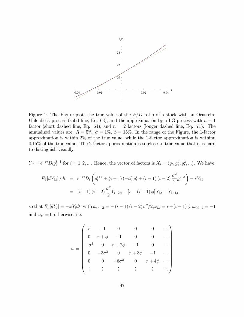
0.04 0.02 0.02 0.04x

20

22

24

PD

Figure 1: The Figure plots the true value of the P/D ratio of a stock with an Ornstein-Uhlenbeck process (solid line, Eq. 63), and the approximation by a LG process with n = 1factor (short dashed line, Eq. 64), and n = 2 factors (longer dashed line, Eq. 71). Theannualized values are: R = 5%, σ = 1%, φ = 15%. In the range of the Figure, the 1-factorapproximation is within 2% of the true value, while the 2-factor approximation is withinn0.15% of the true value. The 2-factor approximation is so close to true value that it is hardto distinguish visually.

Yit = e−rtDtgi−1t for i = 1, 2, .... Hence, the vector of factors is Xt = (gt, g

2t , g

3t , ...). We have:

Et [dYi,t] /dt = e−rtDt

µgi+1t + (i− 1) (−φ) git + (i− 1) (i− 2)

σ2

2gi−3t

¶− rYi,t

= (i− 1) (i− 2) σ2

2Yi−2,t − [r + (i− 1)φ]Yi,t + Yi+1,t

so that Et [dYt] = −ωYtdt, with ωi,i−2 = − (i− 1) (i− 2)σ2/2,ωi,i = r+(i− 1)φ, ωi,i+1 = −1and ωij = 0 otherwise, i.e.

ω =

⎛⎜⎜⎜⎜⎜⎜⎜⎜⎜⎜⎜⎝

r −1 0 0 0 · · ·0 r + φ −1 0 0 · · ·−σ2 0 r + 2φ −1 0 · · ·0 −3σ2 0 r + 3φ −1 · · ·0 0 −6σ2 0 r + 4φ · · ·...

......

......

. . .

⎞⎟⎟⎟⎟⎟⎟⎟⎟⎟⎟⎟⎠47

So the price is:

Pt/Dt = (1, 0, ..., 0, ..)ω−1 ¡1, gt, g2t , ..., gnt , ...¢0 (65)

The sum can be truncated up to step n, i.e. be take to be the restriction of the vector to

the first n dimensions. We compare the LG (65) to the exact expression (113). Numerical

results show that the approximation is very good, even for n = 5.

8.2.2 An improved truncation

There is a better way to truncate the expansion (65). This section is heuristic, not rigorous.

To study the “pure” behavior of the process, with the effect of discounting, we look at the

process when r = 0. Then:

Et [dY2,t] /dt = −φY2t + Y3t (66)

Et [dY3t] /dt = σ2Y1t − 2φY3t + Y4t (67)

Let us study the truncation to 2 terms. We replace Y3 by the value that ensures the terms

in (67) are equal to 0 (that’s the “slaving principle”), so Y3 ' σ2Y1t/ (2φ), and injecting this

in (66), we get: Et [dY2,t] /dt ' σ2Y1t2φ− (φ+R)Y2t. Hence, we approximate the OU process

by the LG process

ω∗(1) =

⎛⎝ r 1

−σ2

2φr + φ

⎞⎠and the corresponding approximation is exactly the one we’ve previously derived, Eq. 64.

We can do the same for higher K’s.For instance, with r = 0, Et [dY4t] /dt = 3σ2Y2t −3φY4t − Y5t, so we replace Y4t ' Y2tσ

2/φ. Injecting this in (67) we get:

ω∗(2) =

⎛⎜⎜⎝r −1 0

0 r + φ −1−σ2 −σ2

φr + 2φ

⎞⎟⎟⎠ (68)

The corresponding approximation is (71) below.

48

Conclusion: The successive approximations, with 0, 1, and 2 factors respectively, are:

V(0)t =

1

R(69)

V(1)t =

1 + xtR+φ

R− σ2

(R+φ)2φ

(70)

V(2)t =

1

R+

gtR (R+ φ)

+g2t +

σ2

Rφ(xt + φ)

R (R+ φ)³R+ 2φ− σ2

Rφ

´ (71)

The approximation is very good. For instance, Figure 1 plots the LG approximation V (2)t ,

and it is extremely close, and very hard to distinguish visually from the true value.

8.3 Conclusion

It would be good to generalize the above procedure, probably in a future paper. It suggests

that LG processes allow the evaluation of the price of many non-LG processes (e.g., those

with analytic expansions), to an arbitrary degree of precision.

9 Twisted vs Non-twisted process

The “twist” term in LG processes may at first glance be strange. On the other hand,

mathematically it is close to a simple AR(1). It may be useful to illustrate, in the same

simulations, how an AR(1) and a LG process behave.

Consider the processes

x∗t+∆t =(1− φ∆t)x∗t + vx∆t

1 + x∗t∆t+ σ (x∗t ) (∆t)1/2 εt+∆t with (72)

xt+∆t = (1− φ∆t)xt + σ (xt) (∆t)1/2 εt+∆t (73)

where εt+∆t is a uniformly distributed, with mean 0 distribution with variance 1. The νx

term is an adjustment convexity, that will be determined very soon, and is analogous to the

“σ2/ (2φ)” in section 8. The processes mean-revert with a speed φ. The starred variables

relate to the LG process, while the non-starred variables relate to the AR(1). The dividends

49

start at D∗0 = D0 = 1, and follow:

Dt+∆t = Dt

¡1 + ηt+∆t

¢(1 + xt∆t) egD∆t

D∗t+∆t = D∗

t

¡1 + ηt+∆t

¢ex∗t∆t+gD∆t

where η has mean 0 and standard deviation ση. In the above expressions, xt is a growth rate.

In another interpretation, useful when purely dealing with a price-dividend ratio, is that xt

is minus a risk premium. Stock prices are the net present value of dividend, discounted with

a risk-neutral rate r.

The variance process is:

σ2 (X) = 2K (1−X/Xmin)2 (1−X/Xmax)

2

withK > 0. It goes to 0 fast enough atXmin andXmax, ensuring that xt is within [Xmin, Xmax].

The average volatility of X is fairly well approximated by: vx = K1/2ξ, with ξ = 1.35, as

proposed in the Appendix to Gabaix (2007), “A Simple, Unified, Exactly Solved Framework

for Ten Puzzles in Macro-Finance”.

For the simulations, each period lasts a month, ∆t = 1/12. I use annual units, and I

take R = r− gD = 0.05, for a central P/D ratio of 20. Also, (Xmin,Xmax) = (−8%, 8%), andφ = 0.15 (which means that xt mean-reverts with a half-life of mean-reversion of 5 years).

Finally, K = 0.1φ |Xmin|Xmax, which corresponds to a annual volatility of the log P/D

ratio of 7% (vx/ (R+ φ)), based solely on the effect mentioned here. It is easy to increase

this volatility, for instance by introducing a positive correlation between innovations to

dividends, and innovations to dividend growth.

I simulate 100 years of data. Figures 2-4 illustrate a typical run. They show xt and x∗t ,

the corresponding price/dividend ratio Pt/Dt and P ∗t /D∗t , and the (log) dividends Dt and

D∗t . (For the LG process, the PD ratio is in closed form; for the AR(1) process, I solve for

it numerically). Given that the processes for xt and x∗t are similar up to second order terms,

they are close, an expectation confirmed by Figure 2. The standard deviation of xt − xt∗ is

about 0.1 standard deviation of xt.

Figure 3 shows the price-dividend ratio of the two processes. They are also reasonably

50

20 40 60 80 100t

0.04

0.02

0.02

0.04

0.06x

Figure 2: Process for xt, simulated over 100 years. The solid black line is the LG process,and dashed purple line is the AR(1). The curves are very close, which was expected as thetwo processes are identical up to second order terms.

20 40 60 80 100t

20

22

24

26

28

PD

Figure 3: The price-dividend ratios, simulated over 100 years. The solid black line representsthe P/D associated with the LG process, and dashed purple line the P/D ratio associatedwith the AR(1) process. The curves are quite close, which makes sense given that the twoprocesses are identical up to second order terms.

51

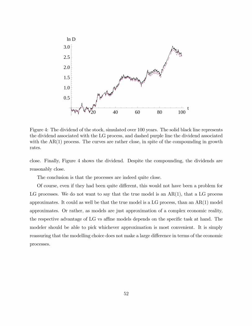
20 40 60 80 100t

0.5

1.0

1.5

2.0

2.5

3.0

ln D

Figure 4: The dividend of the stock, simulated over 100 years. The solid black line representsthe dividend associated with the LG process, and dashed purple line the dividend associatedwith the AR(1) process. The curves are rather close, in spite of the compounding in growthrates.

close. Finally, Figure 4 shows the dividend. Despite the compounding, the dividends are

reasonably close.

The conclusion is that the processes are indeed quite close.

Of course, even if they had been quite different, this would not have been a problem for

LG processes. We do not want to say that the true model is an AR(1), that a LG process

approximates. It could as well be that the true model is a LG process, than an AR(1) model

approximates. Or rather, as models are just approximation of a complex economic reality,

the respective advantage of LG vs affine models depends on the specific task at hand. The

modeler should be able to pick whichever approximation is most convenient. It is simply

reassuring that the modelling choice does not make a large difference in terms of the economic

processes.

52