8. modelling uncertainty - intranet...

8. Modelling Uncertainty

1. Introduction 231

2. Generating Values From Known Probability Distributions 231

3. Monte Carlo Simulation 233

4. Chance Constrained Models 235

5. Markov Processes and Transition Probabilities 236

6. Stochastic Optimization 239

6.1. Probabilities of Decisions 243

6.2. A Numerical Example 244

7. Conclusions 251

8. References 251

wrm_ch08.qxd 8/31/2005 11:55 AM Page 230

1. Introduction

Water resources planners and managers work in an envi-ronment of change and uncertainty. Water supplies arealways uncertain, if not in the short term at least in thelong term. Water demands and the multiple purposesand services water provide are always changing, andthese changes cannot always be predicted. Many of thevalues of parameters of models used to predict the multi-ple hydrological, economic, environmental, ecologicaland social impacts are also changing and uncertain.Indeed models used to predict these impacts are, at leastin part, based on many imprecise assumptions. Planningand managing, given this uncertainty, cannot be avoided.

To the extent that probabilities can be assigned to var-ious uncertain inputs or parameter values, some of thisuncertainty can be incorporated into models. These mod-els are called probabilistic or stochastic models. Most prob-abilistic models provide a range of possible values foreach output variable along with their probabilities.Stochastic models attempt to model the random processesthat occur over time, and provide alternative time seriesof outputs along with their probabilities. In other cases,sensitivity analyses (solving models under differentassumptions) can be carried out to estimate the impact ofany uncertainty on the decisions being considered. Insome situations, uncertainty may not significantly affectthe decisions that should be made. In other situations itwill. Sensitivity analyses can help estimate the extent to

231

Modelling Uncertainty

Decision–makers are increasingly willing to consider the uncertainty associatedwith model predictions of the impacts of their possible decisions. Information onuncertainty does not make decision–making easier, but to ignore it is to ignorereality. Incorporating what is known about the uncertainty into input parametersand variables used in optimization and simulation models can help in quantifyingthe uncertainty in the resulting model predictions – the model output. This chapterdiscusses and illustrates some approaches for doing this.

8

which we need to try to reduce that uncertainty. Modelsensitivity and uncertainty analysis is discussed in moredetail in Chapter 9.

This chapter introduces a number of approaches toprobabilistic optimization and simulation modelling.Probabilistic models will be developed and applied tosome of the same water resources management problemsused to illustrate deterministic modelling in previouschapters. They can be, and have been, applied to numer-ous other water resources planning and managementproblems as well. The purpose here, however, is simply toillustrate some of the commonly used approaches to theprobabilistic modelling of water resources system designand operating problems.

2. Generating Values From KnownProbability Distributions

Variables whose values cannot be predicted with certaintyare called random variables. Often, inputs to hydrologicalsimulation models are observed or synthetically generatedvalues of rainfall or streamflow. Other examples of suchrandom variables could be evaporation losses, point andnon-point source wastewater discharges, demands forwater, spot prices for energy that may impact the amountof hydropower production, and so on. For randomprocesses that are stationary – that is, the statistical attrib-utes of the process are not changing – and if there is

wrm_ch08.qxd 8/31/2005 11:55 AM 31

232 Water Resources Systems Planning and Management

lower and upper limits is equally likely. Using Equation 8.2,together with a series of uniformly distributed (all equallylikely) values of p* over the range from 0 to 1 (that is, alongthe vertical axis of Figure 8.2), one can generate a corre-sponding series of variable values, r*, associated with anydistribution. These random variable values will have acumulative distribution as shown in Figure 8.2, and hencea density distribution as shown in Figure 8.1, regardless ofthe types or shapes of those distributions. The mean,variance and other moments of the distributions will bemaintained.

The mean and variance of continuous distributions are:

∫r fR(r)dr � E[R] (8.3)

∫(r � E[R])2 fR(r)dr � Var[R] (8.4)

The mean and variance of discrete distributions havingpossible values denoted by ri with probabilities pi are:

(8.5)

(8.6)

If a time series of T random variable values, rt, from thesame stationary random variable, R, exists, then the serialor autocorrelations of rt and rt�k in this time series for anypositive integer k can be estimated using:

ρ̂R(k)�

(8.7)

[( [ ])( [ ])] ( [ ])r E R r E R r E RkT k

tt T

τ ττ

� � �� 1

2

1∑ ∑�

� �r E R p Rii

i� �[ ] [ ]∑ 2

Var

r p E Ri ii

� [ ]∑

r

() r

f R

r*

*p

E020

110a

Figure 8.1. Probability density distribution of a random variable R. The probability that R is less than or equal r* is p*.

Figure 8.2. Cumulative distribution function of a randomvariable R showing the probability of any observed value of R being less than or equal to a given value r. The probability of an observed value of R being less than orequal to r* is p*.

no serial correlation in the spatial or temporal sequence of observed values, then such random processes can becharacterized by single probability distributions. Theseprobability distributions are often based on past observa-tions of the random variables. These observations or measurements are used either to define the probabilitydistribution itself or to estimate parameter values of anassumed type of distribution.

Let R be a random variable whose probability densitydistribution, fR(r), is as shown in Figure 8.1. This distri-bution indicates the probability or likelihood of anobserved value of the random variable R being betweenany two values of r on the horizontal axis. For example,the probability of an observed value of R being between 0and r* is p*, the shaded area to the left of r*. The entireshaded area of a probability density distribution, such asshown in Figure 8.1, is 1.

Integrating this function over r converts the densityfunction to a cumulative distribution function, FR(r*),ranging from 0 to 1, as illustrated in Figure 8.2.

(8.1)

Given any value of p* from 0 to 1, one can find its corre-sponding variable value r* from the inverse of the cumu-lative distribution function.

FR�1(p*) � r* (8.2)

From the distribution shown in Figure 8.1, it is obvious that the likelihood of different values of the random variable varies; ones in the vicinity of r* are much more likely to occur than are values at the tails of thedistribution. A uniform distribution is one that looks like arectangle; any value of the random variable between its

f r r R r F rR R

r

( ) Pr( *) ( *)*

d � � �0∫

wrm_ch08.qxd 8/31/2005 11:55 AM Page 232

Modelling Uncertainty 233

The probability density and corresponding cumulativeprobability distributions can be of any shape, not justthose named distributions commonly found in proba-bility and statistics books.

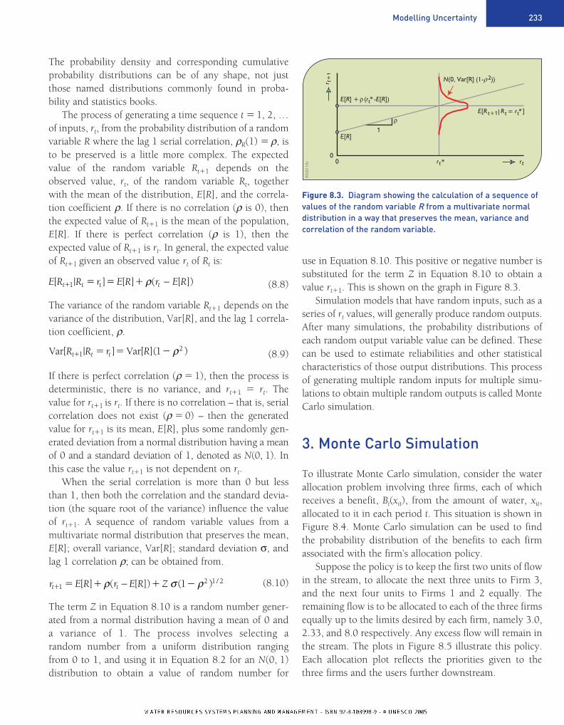
The process of generating a time sequence t � 1, 2, …of inputs, rt, from the probability distribution of a randomvariable R where the lag 1 serial correlation, ρR(1) � ρ, isto be preserved is a little more complex. The expectedvalue of the random variable Rt�1 depends on theobserved value, rt, of the random variable Rt, togetherwith the mean of the distribution, E[R], and the correla-tion coefficient ρ. If there is no correlation (ρ is 0), thenthe expected value of Rt�1 is the mean of the population,E[R]. If there is perfect correlation (ρ is 1), then theexpected value of Rt�1 is rt. In general, the expected valueof Rt�1 given an observed value rt of Rt is:

(8.8)

The variance of the random variable Rt�1 depends on thevariance of the distribution, Var[R], and the lag 1 correla-tion coefficient, ρ.

(8.9)

If there is perfect correlation (ρ � 1), then the process isdeterministic, there is no variance, and rt�1 � rt. Thevalue for rt�1 is rt. If there is no correlation – that is, serialcorrelation does not exist (ρ � 0) – then the generatedvalue for rt�1 is its mean, E[R], plus some randomly gen-erated deviation from a normal distribution having a meanof 0 and a standard deviation of 1, denoted as N(0, 1). Inthis case the value rt�1 is not dependent on rt.

When the serial correlation is more than 0 but lessthan 1, then both the correlation and the standard devia-tion (the square root of the variance) influence the valueof rt�1. A sequence of random variable values from a multivariate normal distribution that preserves the mean,E[R]; overall variance, Var[R]; standard deviation σ, andlag 1 correlation ρ; can be obtained from.

(8.10)

The term Z in Equation 8.10 is a random number gener-ated from a normal distribution having a mean of 0 and a variance of 1. The process involves selecting a random number from a uniform distribution rangingfrom 0 to 1, and using it in Equation 8.2 for an N(0, 1) distribution to obtain a value of random number for

r E R r E R Zt t� � � � �12 1 21[ ] ( [ ]) ( ) /ρ σ ρ−

Var Var[ | ] [ ]( )R R r Rt t t� � � �121 ρ

E R R r E R r E Rt t t t[ | ] [ ] ( [ ])� � � �1 ρ −

use in Equation 8.10. This positive or negative number issubstituted for the term Z in Equation 8.10 to obtain avalue rt�1. This is shown on the graph in Figure 8.3.

Simulation models that have random inputs, such as aseries of rt values, will generally produce random outputs.After many simulations, the probability distributions ofeach random output variable value can be defined. Thesecan be used to estimate reliabilities and other statisticalcharacteristics of those output distributions. This processof generating multiple random inputs for multiple simu-lations to obtain multiple random outputs is called MonteCarlo simulation.

3. Monte Carlo Simulation

To illustrate Monte Carlo simulation, consider the waterallocation problem involving three firms, each of whichreceives a benefit, Bi(xit), from the amount of water, xit,allocated to it in each period t. This situation is shown inFigure 8.4. Monte Carlo simulation can be used to findthe probability distribution of the benefits to each firmassociated with the firm’s allocation policy.

Suppose the policy is to keep the first two units of flowin the stream, to allocate the next three units to Firm 3,and the next four units to Firms 1 and 2 equally. Theremaining flow is to be allocated to each of the three firmsequally up to the limits desired by each firm, namely 3.0,2.33, and 8.0 respectively. Any excess flow will remain inthe stream. The plots in Figure 8.5 illustrate this policy.Each allocation plot reflects the priorities given to thethree firms and the users further downstream.

E020

110c r0

0trt

r t+

1

(r *E[ ] +R ρ t -E[ ])R

E[ ]R

ρ1

*

N(0, Var[R] (1-ρ 2))

r *E[R t=t+1 Rt ]

Figure 8.3. Diagram showing the calculation of a sequence ofvalues of the random variable R from a multivariate normaldistribution in a way that preserves the mean, variance andcorrelation of the random variable.

wrm_ch08.qxd 8/31/2005 11:55 AM Page 233

A simulation model can be created. In each of aseries of discrete time periods t, the flows Qt are drawnfrom a probability distribution, such as from Figure 8.2using Equation 8.2. Once this flow is determined, eachsuccessive allocation, xit, is computed. Once an allocationis made it is subtracted from the streamflow and thenext allocation is made on the basis of that reduced


streamflow, in accordance with the allocation policydefined in Figures 8.5a – d. After numerous time steps,the probability distributions of the allocations to each ofthe firms can be defined.

Figure 8.6 shows a flow chart for this simulationmodel.

Q

x

x

x

E020110

d

tQ 1t

1t

Q

2t

Q 3t2t

3t

3

firm 3B ( 8x -0.5x 2x3t )= 3t 3t

1firm 1B ( 6x -x 2x1t )= 1t 1t

2firm 2B ( 7x - .5x1 2x2t )= 2t 2t

Figure 8.4. Streamflowallocations in each period tresult in benefits, Bi(xit), to eachfirm i. The flows, Qit, at eachdiversion site i are the randomflows Qt less the upstreamwithdrawals, if any.

E020

110e

1210

86420

0 2 4 6 8 10 12 14 16 26

allo

catio

n at

div

ersio

nsit

e:

xt

11

streamflow Q1t

18 20 22 24

Figure 8.5a. Water allocation policy for Firm 1 based on theflow at its diversion site. This policy applies for each period t.

E020

110

f

1210

86420

0 2 4 6 8 10 12 14 16 26

allo

catio

n at

div

ersio

nsit

e:

xt 2

2

streamflow Q2 t

18 20 22 24

Figure 8.5b. Water allocation policy for Firm 2 based onthe flow at its diversion site for that firm. This policyapplies for each period t.

E020

110g

1210

86420

0 2 4 6 8 10 12 14 16 26

allo

catio

n at

div

ersio

nsit

e:

xt 3

3

streamflow Q 3 t

18 20 22 24

Figure 8.5c. Water allocation policy for Firm 3 based on the flow at its diversion site. This policy applies for eachperiod t.

E020

110

h

1210

86420

0 2 4 6 8 10 12 14 16 26

stre

amflo

wat

site

3

streamflow Q 3t

18 20 22 24

Figure 8.5d. Streamflow downstream of site 3 given thestreamflow Q3t at site 3 before the diversion. This applies foreach period t.

wrm_ch08.qxd 8/31/2005 11:55 AM Page 234


E020

110

j stop

start

yesnocalculate andplot probabilitydistributions

compute Qt t= +1

set: t = 1Tmax

maxt = T

datastorage

t(Eq.2) Q1t = Qt

compute(fig. 5a)

x1t

compute(fig. 5c)

x3t

compute(fig. 5b)

x2t

Q2t = Q1t - x1t

Q3t = Q2t - x2t

Figure 8.6. Monte Carlosimulation to determineprobability distributions ofallocations to each of threewater users, as illustrated inFigure 8.4. The dashed linesrepresent information (data)flows.

Having defined the probability distribution of the allocations, based on the allocation policy, one can consider each of the allocations as random variables, X1,X2, and X3 for Firms 1, 2 and 3 respectively.

4. Chance Constrained Models

For models that include random variables, it may beappropriate in some situations to consider constraints thatdo not have to be satisfied all the time. Chance constraintsspecify the probability of a constraint being satisfied, or

the fraction of the time a constraint has to apply.Consider, for example, the allocation problem shown inFigure 8.4. For planning purposes, the three firms maywant to set allocation targets, not expecting to have thosetargets met 100% of the time. To ensure, for example, thatan allocation target, Ti, of firm i will be met at least 90%of the time, one could write the chance constraint:

Pr{Ti � Xi} � 0.90 i � 1, 2 and 3 (8.11)

In this constraint, the allocation target Ti is an unknowndecision-variable, and Xi is a random variable whose distribution has just been computed and is known.

wrm_ch08.qxd 8/31/2005 11:55 AM Page 235

To include chance constraints in optimization models, their deterministic equivalents must be defined.The deterministic equivalents of the three chance con-straints in Equation 8.11 are:

Ti � xit0.10 i � 1, 2 and 3 (8.12)

where xit0.10 is the particular value of the random variable

Xi that is equalled or exceeded 90% of the time. Thisvalue is shown on the probability distribution for Xi inFigure 8.7.

To modify the allocation problem somewhat, assumethe benefit obtained by each firm is a function of its tar-get allocation and that the same allocation target appliesin each time period t. The equipment and labour used inthe firm is presumably based on the target allocations.Once the target is set, assume there are no benefits gainedby excess water allocations. If the benefits obtained are to be based on the target allocations rather than the actual allocations, then the optimization problem isone of finding the values of the three targets that maximizethe total benefits obtained with a reliability of, say, at least 90%.

Maximize�6T1 � T12� � �7T2 � 1.5T2

2� � �8T3 � 0.5T32 �

(8.13)

subject to:

Pr{T1 � T2 � T3 � [Qt � min(Qt, 2)]} � 0.90for all periods t (8.14)

where Qt is the random streamflow variable upstream ofall diversion sites. If the same unconditional probability


distribution of Qt applies for each period t, then only oneEquation 8.14 is needed.

Assuming the value of the streamflow, qt0.10, that is

equalled or exceeded 90% of the time, is greater than 2(the amount that must remain in the stream), the deter-ministic equivalent of chance constraint Equation 8.14 is:

T1 � T2 � T3 � �qt0.10 � min�qt

0.10, 2�� (8.15)

The value of the flow that is equal to or exceeds 90%of the time, qt

0.10, can be obtained from the cumulativedistribution of flows as illustrated in Figure 8.8.

Assume this 90% reliable flow is 8. The deterministicequivalent of the chance constraint Equation 8.9 for allperiods t is simply T1 � T2 � T3 � 6. The optimal solution of the chance-constrained target allocationmodel, Equations 8.8 and 8.9, is, as seen before, T1 � 1,T2 � 1 and T3 � 4. The next step would be to simulatethis problem to see what the actual reliabilities might befor various sequences of flows qt.

5. Markov Processes and TransitionProbabilities

Time-series correlations can be incorporated into models using transition probabilities. To illustrate thisprocess, consider the observed flow sequence shown inTable 8.1.

The estimated mean, variance and correlation coeffi-cient of the observed flows shown in Table 8.1 can be calculated using Equations 8.16, 8.17 and 8.18.

E020

110k

(Xf xi

it)

X it0. 01

0.90

X it

Figure 8.7. Probability density distribution of the randomallocation Xi to firm i. The particular allocation value xit

0.10 hasa 90% chance of being equalled or exceeded, as indicated bythe shaded region.

E020

110m

qt0. 01

0. 01

1.00Pr( qt≤Q ) = FQ (qt )

qt

Figure 8.8. Example cumulative probability distributionshowing the particular value of the random variable, qt

0.10,that is equalled or exceeded 90% of the time.

wrm_ch08.qxd 8/31/2005 11:55 AM Page 236

Table 8.1. Sequence of flows for thirty-one time periods t.


E[Q] � qt/31 � 3.155 (8.16)

Var[Q] � (qt � 3.155)2/30 � 1.95 (8.17)

Lag-one correlation coefficient � ρ

(8.18)

The probability distribution of the flows in Table 8.1 can be approximated by a histogram. Histograms can becreated by subdividing the entire range of random vari-able values, such as flows, into discrete intervals. Forexample, let each interval be two units of flow. Countingthe number of flows in each interval and then dividingthose interval counts by the total number of counts resultsin the histogram shown in Figure 8.9. In this case, just tocompare this with what will be calculated later, the firstflow, q1, is ignored.

Figure 8.9 shows a uniform unconditional probabilitydistribution of the flow being in any of the possible dis-crete flow intervals. It does not show the possibledependency of the probabilities of the random variable

� � �

� �

�( . )( . )

( . ) .

q q

q

t t

t

1 3 155 3 155

3 155 0 50

1

30

1

312

∑

∑

1

31

∑

1

31

∑

value, qt�1, in period t � 1 on the observed random vari-able value, qt, in period t. It is possible that the probabil-ity of being in a flow interval j in period t � 1 depends onthe actual observed flow interval i in period t.

To see if the probability of being in any given intervalof flows is dependent on the past flow interval, one cancreate a matrix. The rows of the matrix are the flow inter-vals i in period t. The columns are the flow intervals j inthe following period t � 1. Such a matrix is shown inTable 8.2. The numbers in the matrix are based on theflows in Table 8.1 and indicate the number of times a flowin interval j followed a flow in interval i.

Given an observed flow in an interval i in period t, theprobabilities of being in one of the possible intervals j inthe next period t � 1 must sum to 1. Thus, each numberin each row of the matrix in Table 8.2 can be divided bythe total number of flow transitions in that row (the sum

periodt

1

2

3

4

5

6

7

8

9

10

E020

827w

flowQt

4.5

5.2

6.0

3.2

4.3

5.1

3.6

4.5

1.8

1.5

periodt

periodt

11

12

13

14

15

16

17

18

19

20

21

22

23

24

25

26

27

28

29

30

31

flowQ

flowQt t

1.8

2.5

2.3

1.8

1.2

1.9

2.5

4.1

4.7

5.6

1.8

1.2

2.5

1.9

3.2

2.5

3.5

2.7

1.5

4.1

4.8

E020

110n qt

prob

abili

ty

0 2 4 6 8 10

Figure 8.9. Histogram showing an equal 1/3 probability thatthe values of the random variable Qt will be in any one of thethree two-flow unit intervals.

E020

827x

flow intervalin :t i

1

2

3

5

3

2

flow intervalin +t

4

4

2

1

3

6

1 2 3j =

Table 8.2. Matrix showing the number of times a flow ininterval i in period t was followed by a flow in interval j inperiod t � 1.

wrm_ch08.qxd 8/31/2005 11:55 AM Page 237

of the number of flows in the row) to obtain the proba-bilities of being in each interval j in t � 1 given a flow in interval i in period t. In this case there are ten flows that followed each flow interval i, hence by dividing each number in each row of the matrix by 10 defines thetransition probabilities Pij.

Pij � Pr{Qt�1 in interval j | Qt in interval i} (8.19)

These conditional or transition probabilities, shown inTable 8.3, correspond to the number of transitions shownin Table 8.2.

Table 8.3 is a matrix of transition probabilities. Thesum of the probabilities in each row equals 1. Matricesof transition probabilities whose rows sum to 1 are alsocalled stochastic matrices or first-order Markov chains.

If each row’s probabilities were the same, this wouldindicate that the probability of observing any flow inter-val in the future is independent of the value of previousflows. Each row would have the same probabilities as theunconditional distribution shown in Figure 8.9. In thisexample the probabilities in each row differ, showing thatlow flows are more likely to follow low flows, and highflows are more likely to follow high flows. Thus the flowsin Table 8.1 are positively correlated, as indeed hasalready determined from Equation 8.18.

Using the information in Table 8.3, one can computethe probability of observing a flow in any interval at anyperiod on into the future given the present flow interval.This can be done one period at a time. For example assumethe flow in the current time period t � 1 is in interval i � 3. The probabilities, PQj,2, of being in any of the three


intervals in the following time period t � 2 are the proba-bilities shown in the third row of the matrix in Table 8.3.

The probabilities of being in an interval j in the follow-ing time period t � 3 is the sum over all intervals i of thejoint probabilities of being in interval i in period t � 2 andmaking a transition to interval j in period t � 3.

Pr{Q3 in interval j} � PQj,3

� Pr{Q2 in interval i}

Pr{Q3 in interval j | Q2 in interval i} (8.20)

The last term in Equation 8.20 is the transition probabil-ity, from Table 8.3, that in this example remains the samefor all time periods t. These transition probabilities,Pr{Qt�1 in interval j | Qt in interval i} can be denoted as Pij.

Referring to Equation 8.19, Equation 8.20 can bewritten in a general form as:

PQj,t�1 � PQitPij for all intervals j and periods t

(8.21)

This operation can be continued to any future time period.Table 8.4 illustrates the results of such calculations for

i∑

i∑

E020

911b

1

2

3

flow interval int + : j

0.5

0.3

0.2

1 2 3

0.4

0.4

0.2

0.1

0.3

0.6

flow intervalin t: i

Table 8.3. Matrix showing the probabilities Pij of having a flowin interval j in period t � 1 given an observed flow in interval iin period t.

E020

827y

tim

e pe

riod

t

1

2

3

4

5

6

7

8

flow interval i

0

0.2

0.28

0.312

0.325

0.330

0.332

0.333

1 2 3

probability PQ it

0

0.2

0.28

0.312

0.325

0.330

0.332

0.333

1

0.6

0.44

0.376

0.350

0.340

0.336

0.334

Table 8.4. Probabilities of observing a flow in any flow interval iin a future time period t given a current flow in interval i � 3.These probabilities are derived using the transition probabilitiesPij in Table 8.3 in Equation 8.21 and assuming the flow intervalobserved in Period 1 is in Interval 3.

wrm_ch08.qxd 8/31/2005 11:55 AM Page 238


up to six future periods, given a present period (t � 1)flow in interval i � 3.

Note that as the future time period t increases, theflow interval probabilities are converging to the uncondi-tional probabilities – in this example 1/3, 1/3, 1/3 – asshown in Figure 8.9. The predicted probability ofobserving a future flow in any particular interval at sometime in the future becomes less and less dependent onthe current flow interval as the number of time periodsincreases between the current period and that future timeperiod.

When these unconditional probabilities are reached,PQit will equal PQi,t�1 for each flow interval i. To findthese unconditional probabilities directly, Equation 8.21can be written as:

PQj � PQiPij for all intervals j (8.22)

Equation 8.22 (less one) along with Equation 8.23 can beused to calculate all the unconditional probabilities PQi

directly.

PQi � 1 (8.23)

Conditional or transition probabilities can be incorpo-rated into stochastic optimization models of waterresources systems.

6. Stochastic Optimization

To illustrate the development and use of stochastic opti-mization models, consider first the allocation of water to asingle user. Assume the flow in the stream where the diver-sion takes place is not regulated and can be described by aknown probability distribution based on historical records.Clearly, the user cannot divert more water than is availablein the stream. A deterministic model would include the con-straint that the diversion x cannot exceed the available waterQ. But Q is a random variable. Some target value, q, of therandom variable Q will have to be selected, knowing thatthere is some probability that in reality, or in a simulationmodel, the actual flow may be less than the selected value q.Hence, if the constraint x � q is binding, the actual alloca-tion may be less than the value of the allocation or diversionvariable x produced by the optimization model.

i∑

i∑

If the value of x affects one of the system’s performanceindicators, such as the net benefits, B(x), to the user, amore accurate estimate of the user’s net benefits will beobtained from considering a range of possible allocationsx, depending on the range of possible values of the ran-dom flow Q. One way to do this is to divide the knownprobability distribution of flows q into discrete ranges, i –each range having a known probability PQi. Designate adiscrete flow qi for each range. Associated with each spec-ified flow qi is an unknown allocation xi. Now the singledeterministic constraint x � q can be replaced with theset of deterministic constraints xi � qi, and the term B(x)in the original objective function can be replaced by itsexpected value, ∑iPQi � B(xi).

Note, when dividing a continuous known probabilitydistribution into discrete ranges, the discrete flows qi,selected to represent each range i having a given proba-bility PQi, should be selected so as to maintain at least themean and variance of that known distribution as definedby Equations 8.5 and 8.6.

To illustrate this, consider a slightly more complexexample involving the allocation of water to consumersupstream and downstream of a reservoir. Both the poli-cies for allocating water to each user and the reservoirrelease policy are to be determined. This example prob-lem is shown in Figure 8.10.

If the allocation of water to each user is to be basedon a common objective, such as the minimization of the total sum, over time, of squared deviations from pre-specified target allocations, each allocation in eachtime period will depend in part on the reservoir storagevolume.

allocation dt

user D

allocation ut

user U

flow Qt

initialstorage St

reservoircapacity K

release R t

E020

110o

Figure 8.10. Example water resources system involving waterdiversions from a river both upstream and downstream of areservoir of known capacity.

wrm_ch08.qxd 8/31/2005 11:55 AM Page 239

Consider first a deterministic model of the above prob-lem, assuming known river flows Qt and upstream anddownstream user allocation targets UTt and DTt in each ofT within-year periods t in a year. Assume the objective isto minimize the sum of squared deviations from actualallocations, ut and dt, and their respective target alloca-tions, UTt and DTt in each within-year period t.

Minimize {(UTt � ut)2 � (DTt � dt)

2} (8.24)

The constraints include:a) Continuity of storage involving initial storage volumesSt, net inflows Qt � ut, and releases Rt. Assuming no losses:

St � Qt � ut � Rt � St�1 for each period t,

T � 1 � 1 (8.25)

b) Reservoir capacity limitations. Assuming a knownactive storage capacity K:

St � K for each period t (8.26)

c) Allocation restrictions. For each period t:

ut � Qt (8.27)

dt � Rt (8.28)

Equations 8.25 and 8.28 could be combined to eliminatethe release variable Rt, since in this problem knowledge ofthe total release in each period t is not required. In thiscase, Equation 8.25 would become an inequality.

The solution of this model, Equations 8.24 – 8.28,would depend on the known variables (the targets UTt

and DTt, flows Qt and reservoir capacity K). It wouldidentify the particular upstream and downstream alloca-tions and reservoir releases in each period t. It would notprovide a policy that defines what allocations and releasesto make for a range of different inflows and initial storagevolumes in each period t. A backward-moving dynamicprogramming model can provide such a policy. Thispolicy will identify the allocations and releases to makebased on various initial storage volumes, St, and flows, Qt,as discussed in Chapter 4.

This deterministic discrete dynamic programmingallocation and reservoir operation model can be written fordifferent discrete values of St from 0 � St � capacity K as:

Ftn(St, Qt) � min�(UTt � ut)

2 � (DTt � dt)2

� Ft�1n�1(St�1, Qt�1)�

t

T

∑


The minimization is over all feasible ut, Rt, dt:

ut � Qt

Rt � St � Qt � ut

Rt � St � Qt � ut � K

dt � Rt

St�1 � St � Qt � ut � Rt (8.29)

There are three variables to be determined at each stage ortime period t in the above dynamic programming model.These three variables are the allocations ut and dt and thereservoir release Rt. Each decision involves three discretedecision-variable values. The functions Ft

n(St, Qt) definethe minimum sum of squared deviations given an initialstorage volume St and streamflow Qt in time period or season t with n time periods remaining until the end ofreservoir operation.

One can reduce this three decision-variable model to a single variable model by realizing that, for any fixeddiscrete pair of initial and final storage volume states,there can be a direct tradeoff between the upstream anddownstream allocations, given the particular streamflowin each period t. Increasing the upstream allocation willdecrease the resulting reservoir inflow, and this in turnwill reduce the release by the same amount. This reducesthe amount of water available to allocate to the down-stream use.

Hence, for this example problem involving theseupstream and downstream allocations, a local optimiza-tion can be performed at each time step t for each combi-nation of storage states St and St�1. This optimizationfinds the allocation decision-variables ut and dt that

minimize(UTt � ut)2 � (DTt � dt)

2 (8.30)

where

ut � Qt (8.31)

dt � St � Qt � ut � St�1 (8.32)

This local optimization can be solved to identify the ut

and dt allocations for each feasible combination of St andSt�1 in each period t.

Given these optimal allocations, the dynamic pro-gramming model can be simplified to include only onediscrete decision-variable, either Rt or St�1. If the decisionvariable St�1 is used in each period t, the releases Rt in

wrm_ch08.qxd 8/31/2005 11:55 AM Page 240


those periods t do not need to be considered. Thus thedynamic programming model expressed by Equations8.29 can be written for all discrete storage volumes St

from 0 to K and for all discrete flows Qt as:

Ftn(St, Qt) � min�(UTt � ut(St, St�1))

2

� (DTt � dt(St, St�1))2 � Ft�1

n�1(St�1, Qt�1)�

The minimization is over all feasible discrete values ofSt�1,

St�1 � K (8.33)

where the functions ut(St, St�1) and dt(St, St�1) have beendetermined using Equations 8.30 – 8.32.

As the total number of periods remaining, n, increases,the solution of this dynamic programming model willconverge to a steady or stationary state. The best finalstorage volume St�1 given an initial storage volume St willprobably differ for each within-year period or season t,but for a given season t it will be the same in successiveyears. In addition, for each storage volume St, streamflow,Qt, and within-year period t, the difference betweenFt

n�T(St, Qt) and Ftn(St, Qt) will be the same constant

regardless of the storage volume St and period t. This constant is the optimal, in this case minimum, annualvalue of the objective function, Equation 8.24.

There could be additional limits imposed on storagevariables and release variables, such as for flood controlstorage or minimum downstream flows, as might beappropriate in specific situations.

The above deterministic dynamic programming model(Equation. 8.33) can be converted to a stochastic model.Stochastic models consider multiple discrete flows as wellas multiple discrete storage volumes, and their probabili-ties, in each period t. A common way to do this is toassume that the sequence of flows follow a first-orderMarkov process. Such a process involves the use of tran-sition or conditional probabilities of flows as defined byEquation 8.20.

To develop these stochastic optimization models, it isconvenient to introduce some additional indices or sub-scripts. Let the index k denote different initial storage volume intervals. These discrete intervals divide the con-tinuous range of storage volume values from 0 to theactive reservoir capacity K. Each Skt is a discrete storagevolume that represents the range of storage volumes ininterval k at the beginning of each period t.

Let the following letter l be the index denoting differ-ent final storage volume intervals. Each Sl,t�1 is a discretevolume that represents the storage volume interval l at theend of each period t or equivalently at the beginning of period t � 1. As previously defined, let the indices iand j denote the different flow intervals, and each discrete flow qit and qj,t�1 represent those flow intervals i and j inperiods t and t � 1 respectively.

These subscripts and the volume or flow intervals theyrepresent are illustrated in Figure 8.11.

With this notation, it is now possible to develop a stochastic dynamic programming model that willidentify the allocations and releases that are to be madegiven both the initial storage volume, Skt, and the flow, qit. It follows the same structure as the determin-istic models defined by Equations 8.30 through 8.32,and 8.33.

To identify the optimal allocations in each period t foreach pair of feasible initial and final storage volumes Skt

and Sl,t�1, and inflows qit, one can solve Equations 8.34through 8.36.

minimize (UTt � ukit)2 � (DTt � dkilt)

2 (8.34)

where

ukit � qit ∀ k, i, t. (8.35)

dkilt � Skt � qit � ukit � Sl,t�1 ∀ feasible k, i, l, t.(8.36)

The solution to these equations for each feasible combi-nation of intervals k, i, l, and period t defines the optimalallocations that can be expressed as ut(k, i) and dt(k, i, l).

The stochastic version of Model 8.33, again expressedin a form suitable for backward-moving discrete dynamicprogramming, can be written for different discrete valuesof Skt from 0 to K and for all qit as:

The minimization is over all feasible discrete values ofSl,t�1

Sl,t�1 � K

Sl,t�1 � Skt � qit (8.37)

F S q UT u k t DT d k i l

P F

tn

kt it t t t t

ijt

( , ) min ( ( , )) ( ( , , ))� � � �

�

2 2

ttn

t j tj

S q��

� �11

1 1 1( , ), ,∑

wrm_ch08.qxd 8/31/2005 11:55 AM Page 241

Each Pijt in the above recursive equation is the known

conditional or transition probability of a flow qj,t�1 withininterval j in period t � 1 given a flow of qit within intervali in period t.

Pijt � Pr{flow qj,t�1 within interval j in t � 1 | flow of qit

within interval i in t}

The sum over all flow intervals j of these conditional prob-abilities times the Ft�1

n�1(Sl,t�1, qj,t�1) values is the expectedminimum sum of future squared deviations from alloca-tion targets with n � 1 periods remaining given an initialstorage volume of Skt and flow of qit and final storage volume of Sl,t�1. The value Ft

n(Skt, qit) is the expected minimum sum of squared deviations from the allocationtargets with n periods remaining given an initial storagevolume of Skt and flow of qit. Stochastic models such asthese provide expected values of objective functions.

Another way to write the recursion equations of thismodel, Equation 8.37, is by using just the indices k andl to denote the discrete storage volume variables Skt

and Sl,t�1 and indices i and j to denote the discrete flowvariables qit and qj,t�1:


such that Sl,t�1 � K

Sl,t�1 � Skt � qit (8.38)

The steady-state solution of this dynamic programmingmodel will identify the preferred final storage volume Sl,t�1 in period t given the particular discrete initial stor-age volume Skt and flow qit. This optimal policy can beexpressed as a function � that identifies the best interval lgiven intervals k, i and period t.

l � �(k, i, t) (8.39)

All values of l given k, i and t, defined by Equation 8.39,can be expressed in a matrix, one for each period t.

Knowing the best final storage volume interval l givenan initial storage volume interval k and flow interval i, the

F k i UT u k t DT d k i l

P F

tn

lt t t t

ijt

t

( , ) min ( ( , )) ( ( , , ))� � � �

� �

2 2

1nn

j

l j�1( , )∑

k

k

k

k

k

= 5

= 4

= 3

= 2

=

storage volume interval S

S

S

S

S

5

4

3

2

t

t

t

t

t1

E020

110p

flow

pro

babi

lity

streamflow Q1 2 3 4 5 6 7 8 9t t t t t t t t t

flow interval2 3 4 5 6 7 8 9

q q q q q q q q q

i = 1

P r{Q

it=

P Qit

}

Pr{ Q

it=

PQit

}

Figure 8.11. Discretization ofstreamflows and reservoirstorage volumes. The areawithin each flow interval i belowthe probability densitydistribution curve is theunconditional probability, PQit,associated with the discrete flow qit.

wrm_ch08.qxd 8/31/2005 11:55 AM Page 242


optimal downstream allocation, dt(k, i), can, like theupstream allocation, be expressed in terms of only k andi in each period t. Thus, knowing the initial storage volume Skt and flow qit is sufficient to define the optimalallocations ut(k, i) and dt(k, i), final storage volume Sl,t�1,and hence the release Rt(k, i).

Skt � qit � ut(k, i) � Rt(k, i) � Sl,t�1 ∀ k, i, t

where l � �(k, i, t) (8.40)

6.1. Probabilities of Decisions

Knowing the function l � �(k, i, t) permits a calculationof the probabilities of the different discrete storage volumes, allocations, and flows. Let

PSkt � the unknown probability of an initial storage volume Skt being within some interval k in period t;

PQit � the steady-state unconditional probability of flowqit within interval i in period t; and

Pkit � the unknown probability of the upstream anddownstream allocations ut(k, i) and dt(k, i) and reservoirrelease Rt(k, i) in period t.

As previously defined,Pij

t � the known conditional or transition probability of aflow within interval j in period t � 1 given a flow withininterval i in period t.

These transition probabilities Pijt can be displayed in

matrices, similar to Table 8.3, but as a separate matrix(Markov chain) for each period t.

The joint probabilities of an initial storage interval k,an inflow in the interval i, Pkit in each period t must sat-isfy two conditions. Just as the initial storage volume inperiod t � 1 is the same as the final storage volume inperiod t, the probabilities of these same respective discrete storage volumes must also be equal. Thus,

(8.41)

where the sums in the right hand side of Equation 8.41are over only those combinations of k and i that result ina final volume interval l. This relationship is defined byEquation 8.39 (l � �(k, i, t)).

While Equation 8.41 must apply, it is not sufficient.The joint probability of a final storage volume in interval

P P l tj tj

kitik

1 1, , ,� �∑ ∑∑ ∀

l in period t and an inflow j in period t � 1 must equal thejoint probability of an initial storage volume in the sameinterval l and an inflow in the same interval j in period t � 1. Multiplying the joint probability Pkit times the con-ditional probability Pij

t and then summing over all k and ithat results in a final storage interval l defines the former,and the joint probability Pl,j,t�1 defines the latter.

Pl,j,t�1 � PkitPijt ∀l, j, t l � �(k, i, t) (8.42)

Once again the sums in Equation 8.42 are over all combi-nations of k and i that result in the designated storage volume interval l as defined by the policy �(k, i, t).

Finally, the sum of all joint probabilities Pkit in eachperiod t must equal 1.

Pkit � 1 ∀t (8.43)

Note the similarity of Equations 8.42 and 8.43 to theMarkov steady-state flow Equations 8.22 and 8.23. Insteadof only one flow interval index considered in Equations8.22 and 8.23, Equations 8.42 and 8.43 include twoindices, one for storage volume intervals and the other forflow intervals. In both cases, one of Equations 8.22 and8.42 can be omitted in each period t since it is redundantwith that period’s Equations 8.23 and 8.43 respectively.

The unconditional probabilities PSkt and PQit can bederived from the joint probabilities Pkit.

PSkt � Pkit ∀k, t (8.44)

PQit � Pkit ∀i, t (8.45)

Each of these unconditional joint or marginal probabili-ties, when summed over all their volume and flowindices, will equal 1. For example,

PSkt � PQit � 1 (8.46)

Note that these probabilities are determined only on thebasis of the relationships among flow and storage intervalsas defined by Equation 8.39, l � �(k, i, t) in each periodt, and the Markov chains defining the flow interval tran-sition or conditional probabilities, Pij

t . It is not necessary toknow the actual discrete storage values representing thoseintervals. Thus assuming any relationship among the stor-age volume and flow interval indices, l � �(k, i, t) and a

i∑

k∑

k∑

i∑

k i∑ ∑

k i∑ ∑

wrm_ch08.qxd 8/31/2005 11:55 AM Page 243

knowledge of the flow interval transition probabilities Pijt ,

one can determine the joint probabilities Pkit and theirmarginal or unconditional probabilities PSkt. One doesnot need to know what those storage intervals are to cal-culate their probabilities.

Given the values of these joint probabilities Pkit, thedeterministic model defined by Equations 8.24 to 8.28can be converted to a stochastic model to identify the beststorage and allocation decision-variable values associatedwith each storage interval k and flow interval i in eachperiod t.

(8.47)

The constraints include:a) Continuity of storage involving initial storage volumesSkt, net inflows qit � ukit, and at least partial releases dkit.Again assuming no losses:

Skt � qit � ukit � dkit � Sl,t�1 ∀k, i, t

l � �(k, i, t) (8.48)

b) Reservoir capacity limitations.

Skit � K ∀k, i, t (8.49)

c) Allocation restrictions.

ukit � qit ∀k, i, t (8.50)

More detail on these and other stochastic modellingapproaches can be found in Faber and Stedinger (2001);Gablinger and Loucks (1970); Huang et al. (1991); Kimand Palmer (1997); Loucks and Falkson (1970);Stedinger et al. (1984); Su and Deininger (1974); Tejada-Guibert et al. (1993 1995); and Yakowitz (1982).

6.2. A Numerical Example

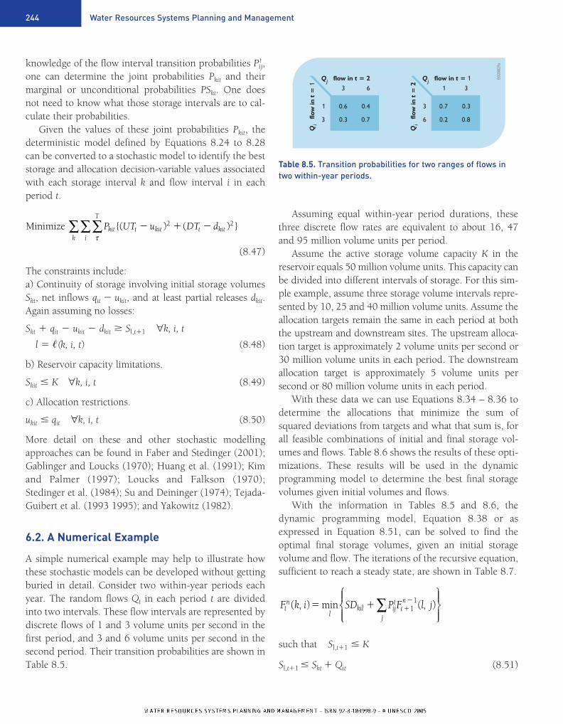
A simple numerical example may help to illustrate howthese stochastic models can be developed without gettingburied in detail. Consider two within-year periods eachyear. The random flows Qt in each period t are dividedinto two intervals. These flow intervals are represented bydiscrete flows of 1 and 3 volume units per second in thefirst period, and 3 and 6 volume units per second in thesecond period. Their transition probabilities are shown inTable 8.5.

Minimize P UT u DT dkit

T

t kitik

t kitτ∑∑∑ {( ) ( ) }� � �2 2


Assuming equal within-year period durations, thesethree discrete flow rates are equivalent to about 16, 47and 95 million volume units per period.

Assume the active storage volume capacity K in thereservoir equals 50 million volume units. This capacity canbe divided into different intervals of storage. For this sim-ple example, assume three storage volume intervals repre-sented by 10, 25 and 40 million volume units. Assume theallocation targets remain the same in each period at boththe upstream and downstream sites. The upstream alloca-tion target is approximately 2 volume units per second or30 million volume units in each period. The downstreamallocation target is approximately 5 volume units per second or 80 million volume units in each period.

With these data we can use Equations 8.34 – 8.36 todetermine the allocations that minimize the sum ofsquared deviations from targets and what that sum is, forall feasible combinations of initial and final storage vol-umes and flows. Table 8.6 shows the results of these opti-mizations. These results will be used in the dynamicprogramming model to determine the best final storagevolumes given initial volumes and flows.

With the information in Tables 8.5 and 8.6, thedynamic programming model, Equation 8.38 or asexpressed in Equation 8.51, can be solved to find theoptimal final storage volumes, given an initial storage volume and flow. The iterations of the recursive equation,sufficient to reach a steady state, are shown in Table 8.7.

such that Sl,t�1 � K

Sl,t�1 � Skt � Qit (8.51)

F k i SD P F l jtn

lkil ij

ttn

j

( , ) min ( , )� � ��11∑

flow in = 2t flow in =t

flow

in=

1t

flow

in=

2t

Qi

Qi

Qj Qj

0.6 0.70.4 0.3

0.3 0.20.7 0.8

3 16 3

1 3

3 6

E020

829a

Table 8.5. Transition probabilities for two ranges of flows intwo within-year periods.

wrm_ch08.qxd 8/31/2005 11:55 AM Page 244


initialstorage

flow finalstorage

intervalindices

upstreamallocation

down-streamallocation

sumsquareddeviationSDd kilkiluS ki1 k i l, ,Q iSk

1010101010101010

252525252525252525

4996.07141.01989.03204.04869.0

112.5450.0

1012.5

3301.04996.07141.01152.01989.03204.0

0.0112.5450.0

16.01.0

47.032.017.072.565.075.5

31.016.0

1.056.047.032.080.072.565.0

0.00.00.00.00.0

22.515.0

7.5

0.00.00.06.00.00.0

30.022.515.0

1, 1, 11, 1, 21, 2, 11, 2, 21, 2, 31, 3, 11, 3, 21, 3, 3

2, 1, 12, 1, 22, 1, 32, 2, 12, 2, 22, 2, 32, 3, 12, 3, 22, 3, 3

1025102540102540

102540102540102540

1616474747959595

161616474747959595

404040404040404040

2056.03301.04996.0

544.51152.01989.0

0.00.0

112.5

46.031.016.063.556.047.080.080.072.5

0.00.00.0

13.56.00.0

30.030.022.5

3, 1, 13, 1, 23, 1, 33, 2, 13, 2, 23, 2, 33, 3, 13, 3, 23, 3, 3

102540102540102540

161616474747959595

E020

829b

Table 8.6. Optimal allocationsassociated with given initial storage,Sk, flow, Qi, and final storage, Sl,volumes. These allocations uki anddkil minimize the sum of squareddeviations, DSkil � (30 � uki)

2

� (80 � dkil)2, from upstream and

downstream targets, 30 and 80respectively, subject to uki � flow Qi,and dkil � release (Sk � Qi � uki � Sl).

the data in Tables 8.5 and 8.8. It is obvious that if thepolicy from Table 8.9 is followed, the steady-state proba-bilities of being in storage Interval 1 in Period 1 and inInterval 3 in Period 2 are 0.

Multiplying these joint probabilities by the correspon-ding SDkit values in the last column of Table 8.6 providesthe annual expected squared deviations, associated withthe selected discrete storage volumes and flows. This isdone in Table 8.11 for those combinations of k, i, and lthat are contained in the optimal solution as listed inTable 8.9.

The sum of products of the last two columns in Table 8.11 for each period t equals the expected squareddeviations in the period. For period t � 1, the expected

This process can continue until a steady-state policy is defined. Table 8.8 summarizes the next five iterations.At this stage, the annual differences in the objective values associated with a particular state and season have come close to a common constant value.

While the differences between corresponding Ftn�T and

Ftn have not yet reached a common constant value to the

nearest unit deviation (they range from, 3475.5 to 3497.1for an average of 3485.7), the policy has converged to thatshown in Tables 8.8 and 8.9.

Given this operating policy, the probabilities of beingin any of these volume and flow intervals can be determined by solving Equations 8.42 through 8.45.Table 8.10 shows the results of these equations applied to

wrm_ch08.qxd 8/31/2005 11:55 AM Page 245


E020

829d

storage& flow optimal

1,1 6234.44996.0 + 0.6 (1989.0) +0.4 (112.5)7141.0 + 0.6 (1152.0) +0.4 ( 0.0)infeasible ----

lll

= 1= 2= 3

SDkil + Σj Pijt Ft+1

n-1(l, j) Ftn (k, i)

k, i

== 7832.2= ---

6234.4

l

1

1,2

2,1

2,2

3,1

3,2

2664.5

4539.4

1827.5

3294.4

1220.0

1989.0 + 0.3 (1989.0) +0.7 (112.5)3204.0 + 0.3 (1152.0) +0.7 ( 0.0)4869.0 + 0.3 ( 544.5) +0.7 ( 0.0)

3301.0 + 0.6 (1989.0) +0.4 (112.5)4996.0 + 0.6 (1152.0) +0.4 ( 0.0)7141.0 + 0.6 ( 544.5) +0.4 ( 0.0)

1152.0 + 0.3 (1989.0) +0.7 (112.5)1989.0 + 0.3 (1152.0) +0.7 ( 0.0)3204.0 + 0.3 ( 544.5) +0.7 ( 0.0)

2056.0 + 0.6 (1989.0) +0.4 (112.5)3301.0 + 0.6 (1152.0) +0.4 ( 0.0)4996.0 + 0.6 ( 544.5) +0.4 ( 0.0)

544.5 + 0.3 (1989.0) +0.7 (112.5)1152.0 + 0.3 (1152.0) +0.7 ( 0.0)1989.0 + 0.3 ( 544.5) +0.7 ( 0.0)

lll

= 1= 2= 3

lll

= 1= 2= 3

lll

= 1= 2= 3

lll

= 1= 2= 3

lll

= 1= 2= 3

== 3549.6= 5032.35

2664.45

== 5687.2= 7467.7

4539.4

== 2334.6= 3367.35

1827.45

== 3992.2= 5322.7

3294.4

== 1497.6= 2152.35

1219.95

1

1

1

1

1

period = 1, = 2t n

E020

829c

storage& flow

period = 2, = 1t n

optimal

1,2 1989.01989.0 + 03204.0 + 04869.0 + 0

lll

= 1= 2= 3



k, i l

1

1,3

2,2

2,3

3,2

3,3

112.5

1152.0

0.0

544.5

0.0

112.5 + 0450.0 + 0

1012.0 + 0

1152.0 + 01989.0 + 03204.0 + 0

0.0 + 0112.5 + 0450.0 + 0

544.5 + 01152.0 + 01989.0 + 0

0.0 + 00.0 + 0

112.5 + 0

lll

= 1= 2= 3

lll

= 1= 2= 3

lll

= 1= 2= 3

lll

= 1= 2= 3

lll

= 1= 2= 3

1

1

1

1

1,2

Table 8.7. First four iterations of dynamicprogramming model, Equations 8.51, movingbackward in successive periods n, beginning inseason t � 2 with n � 1. The iterations stop whenthe final storage policy given any initial storagevolume and flow repeats itself in two successiveyears. Initially, with no more periods remaining,F1

0(k, i) � 0 for all k and i.

(contd.)

wrm_ch08.qxd 8/31/2005 11:55 AM Page 246


Table 8.7. Concluded.

E020

829e


1,26929.8

1989.0 + 0.7 (6234.4) +0.3 (2664.5)3204.0 + 0.7 (4539.4) +0.3 (1827.5)4869.0 + 0.7 (3294.4) +0.3 (1219.9)

lll

= 1= 2= 3



k, i

= 7152.4== 7541.1

6929.8

l

2

1,3

2,2

2,3

3,2

3,3

112.5 + 0.2 (6234.4) +0.8 (2664.5)450.0 + 0.2 (4539.4) +0.8 (1827.5)

1012.5 + 0.2 (3294.4) +0.8 (1219.9)

1152.0 + 0.7 (6234.4) +0.3 (2664.5)1989.0 + 0.7 (4539.4) +0.3 (1827.5)3204.0 + 0.7 (3294.4) +0.3 (1219.9)

0.0 + 0.2 (6234.4) +0.8 (2664.5)112.5 + 0.2 (4539.4) +0.8 (1827.5)450.0 + 0.2 (3294.4) +0.8 (1219.9)

544.5 + 0.7 (6234.4) +0.3 (2664.5)1152.0 + 0.7 (4539.4) +0.3 (1827.5)1989.0 + 0.7 (3294.4) +0.3 (1219.9)

0.0 + 0.2 (6234.4) +0.8 (2664.5)0.0 + 0.2 (4539.4) +0.8 (1827.5)

112.5 + 0.2 (3294.4) +0.8 (1219.9)

lll

= 1= 2= 3

lll

= 1= 2= 3

lll

= 1= 2= 3

lll

= 1= 2= 3

lll

= 1= 2= 3

= 3490.0= 2819.8= 2647.3

= 6315.4== 5876.1

5714.8

= 3378.4= 2482.3= 2084.8

= 5707.9= 4877.8= 4661.1

= 3378.4= 2369.8= 1747.3

3

2

3

3

3

period = 2, = 3t n

2647.3

5714.8

2084.8

4661.1

1747.3

E020

829f


1,1 10212.84996.0 + 0.6 (6929.8) +0.4 (2647.3)7141.0 + 0.6 (5714.8) +0.4 (2084.8)infeasible ---

lll

= 1= 2= 3



k, i

==

l

1

1,2

2,1

2,2

3,1

2,2

1989.0 + 0.3 (6929.8) +0.7 (2647.3)3204.0 + 0.3 (5714.8) +0.7 (2084.8)4869.0 + 0.3 (4661.1) +0.7 (1747.3)

3301.0 + 0.6 (6929.8) +0.4 (2647.3)4996.0 + 0.6 (5714.8) +0.4 (2084.8)7141.0 + 0.6 (4661.1) +0.4 (1747.3)

1152.0 + 0.3 (6929.8) +0.7 (2647.3)1989.0 + 0.3 (5714.8) +0.7 (2084.8)3204.0 + 0.3 (4661.1) +0.7 (1747.3)

2056.0 + 0.6 (6929.8) +0.4 (2647.3)3301.0 + 0.6 (5714.8) +0.4 (2084.8)4996.0 + 0.6 (4661.1) +0.4 (1747.3)

544.5 + 0.3 (6929.8) +0.7 (2647.3)1152.0 + 0.3 (5714.8) +0.7 (2084.8)1989.0 + 0.3 (4661.1) +0.7 (1747.3)

lll

= 1= 2= 3

lll

= 1= 2= 3

lll

= 1= 2= 3

lll

= 1= 2= 3

lll

= 1= 2= 3

===

===

===

===

===

1

1

1

1

2

period = 1, = 4t n

5921.1

8517.8

5084.1

7272.8

4325.8

10212.811403.8

5921.16377.87490.5

8517.89258.8

10636.6

5084.15162.85825.5

7272.87563.88491.6

4476.6

4610.54325.8

wrm_ch08.qxd 8/31/2005 11:55 AM Page 247

sum of squared deviations are 1893.3 and for t � 2 theyare 1591.0. The total annual expected squared deviationsare 3484.3. This compares with the expected squareddeviations derived from the dynamic programmingmodel, after 9 iterations, ranging from 3475.5 to 3497.1(as calculated from data in Table 8.8).

These upstream allocation policies can be displayed inplots, as shown in Figure 8.12.

The policy for reservoir releases is a function not only ofthe initial storage volumes, but also of the current inflow, inother words, the total water available in the period.Reservoir release rule curves such as shown in Figures 4.16or 4.18 now must become two-dimensional. However, theinflow for each period usually cannot be predicted withcertainty at the beginning of each period. In situationswhere the release cannot be adjusted during the period asthe inflow becomes more predictable, the reservoir releasepolicy has to be expressed in a way that can be followedwithout knowledge of the current inflow. One way to dothis is to compute the expected value of the release for eachdiscrete storage volume, and show it in a release rule. Thisis done in Figure 8.13. The probability of each discreterelease associated with each discrete river flow is the proba-bility of the flow itself. Thus, in Period 1 when the storagevolume is 40, the expected release is 46(0.41) � 56(0.59)� 52. These discrete expected releases can be used to definea continuous range of releases for the continuous range ofstorage volumes from 0 to full capacity, 50. Figure 8.13 also


shows the hedging that might take place as the reservoirstorage volume decreases.

Another approach to defining the releases in eachperiod in a manner that is not dependent on knowledgeof the current inflow, even though the model usedassumes this, is to attempt to define either release targetswith constraints on final storage volumes, or final storagetargets with constraints on total releases. Obviously, suchpolicies will not guarantee constant releases throughouteach period. For example, consider the optimal policyshown in Table 8.9. The releases (or final storage vol-umes) in each period are dependent on the initial storageand current inflow. However, this operating policy can beexpressed as:

• If in period 1, the final storage target should be ininterval 1. Yet the total release cannot exceed the flowin interval 2.

• If in period 2 and the initial storage is in interval 1, therelease should be in interval 1.

• If in period 2 and the initial storage is in interval 2, therelease should be in interval 2.

• If in period 2 and the initial storage is in interval 3, therelease should equal the inflow.

This policy can be followed without any forecast of cur-rent inflow. It will provide the releases and final storagevolumes that would be obtained with a perfect inflowforecast at the beginning of each period.

E020

829g

storage& flow Ft

n (k, i)k, i

1,11,2 10691.7 21,3 5927.7 3

= 2, = 5t n

l*

13782.1 17279.2

Ftn (k, i) Ft

n (k, i) Ftn (k, i) Ft

n (k, i)= 1, = 6t n = 2, = 7t n = 1, = 8t n = 2, = 9t n

l* l* l*l*

1 19345.9 14217.7 12821.4 17708.3

9381.5 12861.31 12 2

3 3

2,1

3,1

2,2

3,2

9476.7

8377.7

2

3

2,3

3,3

5365.2

5027.7

3

3

12087.1

10842.1

15584.2

14339.2

1 1

1 1

8508.9

7750.7

13002.7

11903.7

11984.4

11226.1

16493.2

15394.3

8819.0

8481.5

12298.7

11961.2

1 1

2 2

2 2

3 3

3

3

3

3

Table 8.8. Summary of objectivefunction values Ft

n(k, i) andoptimal decisions for stages n � 5 to 9 periods remaining.

wrm_ch08.qxd 8/31/2005 11:55 AM Page 248


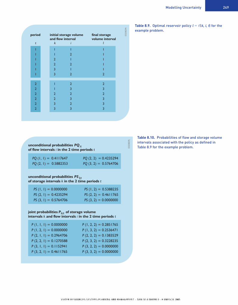
period initial storage volumeand flow interval

final storagevolume interval

kt i l

1 1 1 111111

12233

21212

11112

2 1 2 222222

12233

32323

32333

E020

829h

Table 8.9. Optimal reservoir policy l � �(k, i, t) for theexample problem.

PQ (1, 1) = 0.4117647 PQ (2, 2) = 0.4235294PQ (2, 1) = 0.5882353 PQ (3, 2) = 0.5764706

PS (1, 1) = 0.0000000 PS (1, 2) = 0.5388235PS (2, 1) = 0.4235294 PS (2, 2) = 0.4611765PS (3, 1) = 0.5764706 PS (3, 2) = 0.0000000

P (1, 1, 1) = 0.0000000 P (1, 2, 2) = 0.2851765P (1, 2, 1) = 0.0000000 P (1, 3, 2) = 0.2536471P (2, 1, 1) = 0.2964706 P (2, 2, 2) = 0.1383529P (2, 2, 1) = 0.1270588 P (2, 3, 2) = 0.3228235P (3, 1, 1) = 0.1152941 P (3, 2, 2) = 0.0000000P (3, 2, 1) = 0.4611765 P (3, 3, 2) = 0.0000000

unconditional probabilitiesof flow intervals in the 2 time periodsi t

PQ it

unconditional probabilitiesof storage intervals in the 2 time periodsk t

PS kt

joint probabilities P

intervals k and flow intervals in the 2 time periods tikit of storage volume

E020

829j

Table 8.10. Probabilities of flow and storage volumeintervals associated with the policy as defined in Table 8.9 for the example problem.

wrm_ch08.qxd 8/31/2005 11:55 AM Page 249


init

ial

stor

age

flow

final

stor

age

inte

rval

indi

ces

sum

squ

ared

devi

atio

ns

join

tpr

obab

ility

SDd kitkituS kit1 k i l, ,Q iSk

E020

829k

1010

25254040

101025254040

1647

16471647

479547954795

1010

10101025

252525404040

1,1,11,2,1

2,1,12,2,13,1,13,2,2

1,2,21,3,22,2,2

2,3,33,2,33,3,3

11

1111

222222

0.00.0

0.06.00.06.0

0.07.50.0

15.00.0

22.5

16.047.0

31.056.046.056.0

32.057.547.0

65.047.072.5

4996.01989.0

3301.01152.02056.01152.0

3204.0

1012.51989.0

450.01989.0

112.5

0.00.0

0.29647060.1270588

0.11529410.4611765

0.2851765

0.25364710.13835290.32282350.00.0

1.0

1.0

sum =

sum =

tim

e pe

riod

Pkit

opti

mal

allo

cati

on

Table 8.11. The optimaloperating policy and theprobability of each state anddecision.

river flow

river flow

100

100

25

20

15

10

5

0

25

20

15

10

5

0

upst

ream

use

ral

loca

tion

in p

erio

d 2

upst

ream

use

ral

loca

tion

in p

erio

d1

90

90

80

80

70

70

60

60

50

50

40

40

30

30

20

20

10

10

0

0

22.5

15.0

7.5 stor

age

volu

me

inde

pend

ent o

fst

orag

e vo

lum

e

E020110

q

Figure 8.12. Upstream user allocation policies. In Period 1they are independent of the downstream initial storagevolumes. In Period 2 the operator would interpolate betweenthe three allocation functions given for the three discreteinitial reservoir storage volumes.

504540353025201510

50

stor

age

volu

me

reservoir releases

period

E020110

r

10

20

30

424446

48

50

52

54

period 2

4

53

55

57

59

6162

1628

40

6364

49

55

40

0

60

65

52

0

Figure 8.13. Reservoir release rule showing an interpolatedrelease, increasing as storage volumes increase.

wrm_ch08.qxd 8/31/2005 11:55 AM Page 250


Alternatively, in each period t one can solve themodel defined by Equation 8.37 to obtain the best deci-sion for the current and a sequence of future periods,taking into account all current information regardingthe objectives and possible inflow scenarios and theirprobabilities. The actual release decision in the currentperiod can be the expected value of all these releases inthis current period. At the beginning of the next period,the model is updated with respect to current initialstorage and inflow scenarios (as well as any changes inobjectives or other constraints) and solved again. Thisprocess continues in real time. This approach is dis-cussed in Tejada-Guibert et al. (1993) and is the cur-rent approach for providing release advice to the Boardof Control that oversees the releases from Lake Ontariothat govern the water levels of the lake and the St. Lawrence River.

These policies, and modifications of them, can be simulated to determine improved release rules.

7. Conclusions

This chapter has introduced some approaches for includ-ing risk in optimization and simulation models. The dis-cussion began with ways to obtain values of randomvariables whose probability distributions are known.These values, for example streamflows or parameter val-ues, can be inputs to simulation models. Monte Carlosimulation involves the use of multiple simulations usingthese random variable values to obtain the probabilitydistributions of outputs, including various system per-formance indicators.

Two methods were reviewed for introducing random variables along with their probabilities into opti-mization models. One involves the use of chance con-straints. These are constraints that must be met, as allconstraints must, but now with a certain probability. As inany method there are limits to the use of chance con-straints. These limitations were not discussed, but in caseswhere chance constraints are applicable, and if their deter-ministic equivalents can be defined, they are probably theonly method of introducing risk into otherwise determin-istic models that do not add to the model size.

Alternatively, the range of random variable values can be divided into discrete ranges. Each range can be

represented by a specific or discrete value of the random variable. These discrete values and their proba-bilities can become part of an optimization model. Thiswas demonstrated by means of transition probabilitiesincorporated into both linear and dynamic programmingmodels.

The examples used in this chapter to illustrate thedevelopment and application of stochastic optimizationand simulation models are relatively simple. These andsimilar probabilistic and stochastic models have beenapplied to numerous water resources planning and man-agement problems. They can be a much more effectivescreening tool than deterministic models based on themean or other selected values of random variables. Butsometimes they are not. Clearly if the system beinganalysed is very complex, or just very big in terms of thenumber of variables and constraints, the use of determin-istic models for a preliminary screening of alternativesprior to a more precise probabilistic screening is oftenwarranted.

8. References

FABER, B.A. and STEDINGER, J.R. 2001. Reservoiroptimization using sampling SDP with ensemblestreamflow prediction (ESP) forecasts. Journal ofHydrology, Vol. 249, Nos. 1–4, pp. 113–33.

GABLINGER, M. and LOUCKS, D.P. 1970. Markovmodels for flow regulation. Journal of the HydraulicsDivision, ASCE, Vol. 96, No. HY1, pp. 165–81.

HUANG, W.C.; HARBO, R. and BOGARDI, J.J. 1991. Testing stochastic dynamic programming modelsconditioned on observed or forecast inflows. Journal of WaterResources Planning and Management, Vol. 117, No.1, pp. 28–36.

KIM, Y.O.; PALMER, R.N. 1997. Value of seasonal flowforecasts in bayesian stochastic programming. Journal of Water Resources Planning and Management, Vol. 123,No. 6, pp. 327–35.

LOUCKS, D.P. and FALKSON, L.M. 1970. Comparisonof some dynamic, linear, and policy iteration methodsfor reservoir operation. Water Resources Bulletin, Vol. 6, No. 3, pp. 384–400.

wrm_ch08.qxd 8/31/2005 11:55 AM Page 251

STEDINGER, J.R.; SULE, B.F. and LOUCKS, D.P. 1984.Stochastic dynamic programming models for reservoiroperation optimization. Water Resources Research, Vol. 20,No. 11, pp. 1499–505.

SU, S.Y. and DEININGER, R.A. 1974. Modeling theregulation of lake superior under uncertainty of futurewater supplies. Water Resources Research, Vol. 10, No. 1,pp. 11–22.

TEJADA-GUIBERT, J.A.; JOHNSON, S.A. and STE-DINGER, J.R. 1993. Comparison of two approaches forimplementing multi-reservoir operating policies derivedusing dynamic programming. Water Resources Research,Vol. 29, No. 12, pp. 3969–80.

TEJADA-GUIBERT, J.A.; JOHNSON, S.A. and STEDINGER,J.R. 1995. The value of hydrologic information in stochasticdynamic programming models of a multi-reservoir system.Water Resources Research, Vol. 31, No. 10, pp. 2571–9.

YAKOWITZ, S. 1982. Dynamic programmingapplications in water resources. Water ResourcesResearch, Vol. 18, No. 4, pp. 673–96.

Additional References (Further Reading)

BASSSON, M.S.; ALLEN, R.B.; PEGRAM, G.G.S. andVAN ROOYEN, J.A. 1994. Probabilistic management ofwater resource and hydropower systems. Highlands Ranch,Colo., Water Resources Publications.

BIRGE, J.R. and LOUVEAUX, F. 1997. Introduction tostochastic programming. New York, Springer-Verlag.

DEGROOT, M.H. 1980. Optimal statistical decisions. NewYork, McGraw-Hill.

DEMPSTER, M.A.H. (ed.). 1980. Stochastic programming. New York, Academic Press.

DORFMAN, R.; JACOBY, H.D. and THOMAS, H.A. Jr.1972. Models for managing regional water quality.Cambridge, Mass., Harvard University Press.

ERMOLIEV, Y. 1970. Methods of stochastic programming.Moscow, Nauka. (In Russian.)


ERMOLIEV, Y. and WETS, R., (eds.). 1988. Numericaltechniques for stochastic optimization. Berlin Springer-Verlag.

HEYMAN, D.P. and SOBEL, M.J. 1984. Stochastic modelsin operations research. Vol. 2: Stochastic optimization. NewYork, McGraw-Hill.

HILLIER, F.S. and LIEBERMAN, G.J. 1990. Introductionto stochastic models in operations research. New York,McGraw-Hill.

HOWARD, R.A. 1960. Dynamic programming and Markovprocesses. Cambridge, Mass., MIT Press.

HUFSCHMIDT, M.M. and FIERING, M.B. 1966.Simulation techniques for design of water-resource systems.Cambridge, Mass., Harvard University Press.

LOUCKS, D.P.; STEDINGER, J.S. and HAITH, D.A.1981. Water resource systems planning and analysis.Englewood Cliffs, N.J., Prentice Hall.

MAASS, A.; HUFSCHMIDT, M.M.; DORFMAN, R.;THOMAS, H.A. Jr.; MARGLIN, S.A. and FAIR, G.M.1962. Design of water-resource systems. Cambridge, Mass.,Harvard University Press.

PRÉKOPA, A. 1995. Stochastic programming. Dordrecht,Kluwer Academic.

RAIFFA, H. and SCHLAIFER, R. 1961. Applied statisticaldecision theory. Cambridge, Mass., Harvard University Press.

REVELLE, C. 1999. Optimizing reservoir resources. NewYork, Wiley.

ROSS, S.M. 1983. Introduction to stochastic dynamicprogramming. New York, Academic Press.

SOMLYÓDY, L. and WETS, R.J.B. 1988. Stochasticoptimization models for lake eutrophication management.Operations Research, Vol. 36, No. 5, pp. 660–81.

WETS, R.J.B. 1990 Stochastic programming. In: G.L.Nemhauser, A.H.G. Rinnoy Kan and M.J. Todd (eds.),Optimization: handbooks in operations research and managementscience, Vol. 1, pp. 573–629. Amsterdam, North-Holland.

WURBS, R.A. 1996. Modeling and analysis of reservoirsystem operations. Upper Saddle River, N.J., Prentice Hall.

wrm_ch08.qxd 8/31/2005 11:55 AM Page 252

wrm_ch08.qxd 8/31/2005 11:55 AM Page 253

8. modelling uncertainty - intranet...

Documents