linear and log-linear models for count time series analysiscj82pd40g/fulltext.pdf · linear and...
TRANSCRIPT

Linear and Log-Linear Models for Count Time Series Analysis
A Thesis Presented
by
Nicholas Michael Bosowski
to
The Department of Electrical and Computer Engineering
in partial fulfillment of the requirements
for the degree of
Master of Science
in
Electrical and Computer Engineering
Northeastern University
Boston, Massachusetts
August 2016

To my family.
ii

Contents
List of Figures v
List of Tables vii
List of Acronyms ix
Acknowledgments xi
Abstract of the Thesis xii
1 Introduction 11.1 Motivation . . . . . . . . . . . . . . . . . . . . . . . . . . . . . . . . . . . . . . . 1
1.1.1 Integer Generalized Auto-Regressive Conditional Heteroskedastic Models . 21.2 Objectives and Approach . . . . . . . . . . . . . . . . . . . . . . . . . . . . . . . 3
2 Mathematical Preliminaries 42.1 Probability Distributions . . . . . . . . . . . . . . . . . . . . . . . . . . . . . . . 4
2.1.1 The Normal Distribution . . . . . . . . . . . . . . . . . . . . . . . . . . . 52.1.2 The Gamma Distribution . . . . . . . . . . . . . . . . . . . . . . . . . . . 52.1.3 The Poisson Distribution . . . . . . . . . . . . . . . . . . . . . . . . . . . 72.1.4 The Negative Binomial Distribution . . . . . . . . . . . . . . . . . . . . . 82.1.5 Zero-Inflated Distributions . . . . . . . . . . . . . . . . . . . . . . . . . . 10
2.2 Time Series . . . . . . . . . . . . . . . . . . . . . . . . . . . . . . . . . . . . . . 12
3 Linear and Log-Linear Count Time Series Models 143.1 Auto-Regressive Moving-Average Models . . . . . . . . . . . . . . . . . . . . . . 143.2 Linear Count Models . . . . . . . . . . . . . . . . . . . . . . . . . . . . . . . . . 163.3 The Poisson Linear Model . . . . . . . . . . . . . . . . . . . . . . . . . . . . . . 223.4 The Negative Binomial Two (NB2) Linear Model . . . . . . . . . . . . . . . . . . 303.5 Zero-Inflated Linear Models . . . . . . . . . . . . . . . . . . . . . . . . . . . . . 363.6 The Linear Zero-Inflated Poisson (ZIP) Integer Generalized Auto-Regressive Condi-
tional Heteroscedastic (INGARCH) Model . . . . . . . . . . . . . . . . . . . . . . 393.7 The Linear Zero-Inflated Negative Binomial (ZINB2) Model . . . . . . . . . . . . 443.8 The Log-Linear Model . . . . . . . . . . . . . . . . . . . . . . . . . . . . . . . . 49
iii

3.9 Conclusion . . . . . . . . . . . . . . . . . . . . . . . . . . . . . . . . . . . . . . 50
4 Parameter Estimation in Count Time Series Models 544.1 Introduction . . . . . . . . . . . . . . . . . . . . . . . . . . . . . . . . . . . . . . 544.2 Linear Count Time Series Model Estimation . . . . . . . . . . . . . . . . . . . . . 564.3 Poisson Linear Model Estimation . . . . . . . . . . . . . . . . . . . . . . . . . . . 574.4 Negative Binomial Linear Model Estimation . . . . . . . . . . . . . . . . . . . . . 704.5 Linear Zero-Inflated Poisson Model Estimation . . . . . . . . . . . . . . . . . . . 784.6 Linear Zero-Inflated Negative Binomial Estimation . . . . . . . . . . . . . . . . . 854.7 Log-Linear Model Estimation . . . . . . . . . . . . . . . . . . . . . . . . . . . . 894.8 Conclusion . . . . . . . . . . . . . . . . . . . . . . . . . . . . . . . . . . . . . . 106
5 Count Time Series Forecasting 1075.1 Auto-Regressive Moving Average (ARMA) Forecasts . . . . . . . . . . . . . . . . 1105.2 Linear and Log-Linear Forecasting . . . . . . . . . . . . . . . . . . . . . . . . . . 1115.3 Probabilistic Forecast Assessment . . . . . . . . . . . . . . . . . . . . . . . . . . 111
5.3.1 Calibration and Sharpness . . . . . . . . . . . . . . . . . . . . . . . . . . 1115.3.2 Assessing Probabilistic Calibration: The Probability Integral Transform . . 1135.3.3 Assessing Marginal Calibration: Marginal Calibration Plots . . . . . . . . 1155.3.4 Assessing Sharpness: Scoring Rules . . . . . . . . . . . . . . . . . . . . . 116
5.4 Case Study . . . . . . . . . . . . . . . . . . . . . . . . . . . . . . . . . . . . . . 1195.5 Conclusion . . . . . . . . . . . . . . . . . . . . . . . . . . . . . . . . . . . . . . 121
6 Conclusions 124
Bibliography 127
A Model Correlation 129A.1 The Linear (1,0) Model . . . . . . . . . . . . . . . . . . . . . . . . . . . . . . . . 129A.2 The Linear (1,1) model . . . . . . . . . . . . . . . . . . . . . . . . . . . . . . . . 132A.3 Linear Zero-Inflated (1,0) Model . . . . . . . . . . . . . . . . . . . . . . . . . . . 136
B Model Estimation 139B.1 Poisson . . . . . . . . . . . . . . . . . . . . . . . . . . . . . . . . . . . . . . . . 139B.2 Negative Binomial . . . . . . . . . . . . . . . . . . . . . . . . . . . . . . . . . . 140B.3 ZIP . . . . . . . . . . . . . . . . . . . . . . . . . . . . . . . . . . . . . . . . . . 141B.4 ZINB2 . . . . . . . . . . . . . . . . . . . . . . . . . . . . . . . . . . . . . . . . . 147
iv

List of Figures
1.1 Example Time Series . . . . . . . . . . . . . . . . . . . . . . . . . . . . . . . . . 2
2.1 Examples of the normal distribution. . . . . . . . . . . . . . . . . . . . . . . . . . 52.2 Examples of the Gamma Distribution. . . . . . . . . . . . . . . . . . . . . . . . . 62.3 Comparison of the Gamma Distribution and the Normal Distribution. . . . . . . . 72.4 Examples of The Poisson Distribution. . . . . . . . . . . . . . . . . . . . . . . . . 82.5 Examples of the Negative Binomial Distribution . . . . . . . . . . . . . . . . . . . 102.6 Examples of the Zero-Inflated Poisson and Negative Binomial Distributions. . . . . 12
3.1 Parameter Space of the linear (1,1) model in ARMA space. . . . . . . . . . . . . . 213.2 Parameter space of the linear (1,1) model in ACF space. . . . . . . . . . . . . . . . 213.3 Examples of the Poisson (1,0) Linear Model. . . . . . . . . . . . . . . . . . . . . 233.4 Examples of the Poisson (1,1) Linear Model. . . . . . . . . . . . . . . . . . . . . 243.5 Normalized Error of the Approximate Marginal Distribution of the Poisson (1,0)
Linear Model. . . . . . . . . . . . . . . . . . . . . . . . . . . . . . . . . . . . . . 283.6 Normalized Error of the Approximate Marginal Distribution of the Poisson (1,1)
Linear Model. . . . . . . . . . . . . . . . . . . . . . . . . . . . . . . . . . . . . . 293.7 Constraint on the Dispersion Parameter for the NB2 (1,0) Linear Model . . . . . . 323.8 Constraint on the Dispersion Parameter for the NB2 (1,1) Linear Model . . . . . . 333.9 Examples of the NB2 (1,0) Linear Model . . . . . . . . . . . . . . . . . . . . . . 343.10 Examples of the NB2 (1,1) Linear Model . . . . . . . . . . . . . . . . . . . . . . 353.11 Constraints of the Zero-Inflation Parameter of the ZIP (1,0) model. . . . . . . . . . 413.12 Constraint on the Zero-Inflation Parameter of the ZIP (1,1) model. . . . . . . . . . 413.13 Examples of the ZIP (1,0) model. Each plot shows from top right clockwise: xn
in red and λn in blue; The expected and observed ACF of Xn; The expected andobserved cross-correlation function of Xn and Λn; the expected and observed ACFof Λn; and the marginal distribution of a time series of length 1 million . . . . . . 42
3.14 Examples of the ZIP (1,1) model. Each plot shows from top right clockwise: xnin red and λn in blue; The expected and observed ACF of Xn; The expected andobserved cross-correlation function of Xn and Λn; the expected and observed ACFof Λn; and the marginal distribution of a time series of length 1 million . . . . . . 43
3.15 Minimum allowable value of ν for the ZINB2 (1,0) as a function of p0 and a. . . . 45
v

3.16 Examples of the ZINB2 (1,0) model. Each plot shows from top right clockwise: xnin red and λn in blue; The expected and observed ACF of Xn; The expected andobserved cross-correlation function of Xn and Λn; the expected and observed ACFof Λn; and the marginal distribution of a time series of length 1 million . . . . . . 46
3.17 Examples of the ZINB2 (1,1) model. Each plot shows from top right clockwise: xnin red and λn in blue; The expected and observed ACF of Xn; The expected andobserved cross-correlation function of Xn and Λn; the expected and observed ACFof Λn; and the marginal distribution of a time series of length 1 million . . . . . . 47
3.18 Examples of the ZIP and ZINB2 (1,0) and (1,1) model with regressive parametersoutside the stationarity space of the linear models. From top right clockwise thegroups of plots show: the ZIP (1,0) model; the ZIP (1,1) model; the ZINB2 (1,1)model; the ZINB2 (1,0) model. . . . . . . . . . . . . . . . . . . . . . . . . . . . . 48
3.19 Examples of the log-linear Poisson (1,0) model. . . . . . . . . . . . . . . . . . . . 513.20 Examples of the log-linear Poisson (1,1) model. . . . . . . . . . . . . . . . . . . . 523.21 Examples of the log-linear ZIP(1,1) model. . . . . . . . . . . . . . . . . . . . . . 53
4.1 Error of the Approximate Information Matrix of the Poisson (1,0) model. . . . . . 614.2 Error of the Inverted Approximate Information Matrix of the Poisson (1,0) model. . 624.3 Contour plot of the error of the approximate information matrix for the Poisson (1,1)
model. . . . . . . . . . . . . . . . . . . . . . . . . . . . . . . . . . . . . . . . . . 69
5.1 An example of a point estimate. . . . . . . . . . . . . . . . . . . . . . . . . . . . 1085.2 An example of a forecast estimate. . . . . . . . . . . . . . . . . . . . . . . . . . . 1095.3 Example of the PIT histogram. . . . . . . . . . . . . . . . . . . . . . . . . . . . . 1145.4 An example of how the PIT can be deceptive. . . . . . . . . . . . . . . . . . . . . 1155.5 Example marginal calibration plot. . . . . . . . . . . . . . . . . . . . . . . . . . . 1165.6 Monthly nuclear tests conducted by the United States between 1945 and 1992. . . . 1215.7 Case study residual auto-correlations. . . . . . . . . . . . . . . . . . . . . . . . . 1225.8 Case study PIT histograms. . . . . . . . . . . . . . . . . . . . . . . . . . . . . . . 1225.9 Case study marginal calibration plot. . . . . . . . . . . . . . . . . . . . . . . . . . 123
vi
List of Tables
3.1 Covariance and ACF of the linear (1,0) and (1,1) models. Under the assumption ofuncorrelated errors the ACF is independent of the conditional distribution. . . . . 19
3.2 Dynamics of the Poisson (1,0) and (1,1) linear models. . . . . . . . . . . . . . . . 253.3 Dynamics of the NB2 (1,0) and (1,1) linear models. . . . . . . . . . . . . . . . . 313.4 Dynamics of the zero-inflated linear (1,0) linear models . . . . . . . . . . . . . . 383.5 Dynamics of the ZIP (1,0) and (1,1) linear models . . . . . . . . . . . . . . . . . . 403.6 Dynamics of the ZINB2 (1,0) and (1,1) linear models . . . . . . . . . . . . . . . . 45
4.1 Standard errors of the approximate information matrix for the Poisson (1,0) Modelvs. observed standard errors. . . . . . . . . . . . . . . . . . . . . . . . . . . . . . 60
4.2 Standard errors of the approximate information matrix for the Poisson(1,1) model vs.observed standard errors for d = .5. . . . . . . . . . . . . . . . . . . . . . . . . . 65
4.3 Standard errors of the approximate information matrix for the Poisson(1,1) model vs.observed standard errors for d = 5. . . . . . . . . . . . . . . . . . . . . . . . . . . 65
4.4 Standard errors of the approximate information matrix for the Poisson(1,1) model vs.observed standard errors for d = 10. . . . . . . . . . . . . . . . . . . . . . . . . . 66
4.5 CMLE results of the Poisson linear (1,0) model. . . . . . . . . . . . . . . . . . . . 674.6 CMLE results of the Poisson linear (2,0) model. . . . . . . . . . . . . . . . . . . . 684.7 CMLE results of the Poisson linear (1,1) model. . . . . . . . . . . . . . . . . . . . 684.8 CMLE results of the NB2 linear (1,0) model. . . . . . . . . . . . . . . . . . . . . 744.9 CMLE results of the NB2 linear (2,0) model. . . . . . . . . . . . . . . . . . . . . 744.10 CMLE results of the NB2 linear (1,1) model. . . . . . . . . . . . . . . . . . . . . 754.11 CMLE results of the NB2 linear (1,0) model. . . . . . . . . . . . . . . . . . . . . 754.12 CMLE results of the NB2 linear (2,0) model. . . . . . . . . . . . . . . . . . . . . 764.13 CMLE results of the NB2 linear (1,1) model. . . . . . . . . . . . . . . . . . . . . 764.14 Observed and conditional information matrices of the NB2 linear(1,1) model with
different sample sizes. . . . . . . . . . . . . . . . . . . . . . . . . . . . . . . . . . 774.15 CMLE results of the ZIP linear (1,0) model. . . . . . . . . . . . . . . . . . . . . . 824.16 CMLE results of the ZIP linear (2,0) model. . . . . . . . . . . . . . . . . . . . . . 824.17 CMLE results of the ZIP linear (1,1) model. . . . . . . . . . . . . . . . . . . . . . 834.18 Observed and conditional information matrices of the ZIP linear (1,1) model with
different sample sizes. . . . . . . . . . . . . . . . . . . . . . . . . . . . . . . . . . 844.19 CMLE results of the ZINB2 linear (1,0) model. . . . . . . . . . . . . . . . . . . . 87
vii

4.20 CMLE results of the ZINB2 linear (2,0) model. . . . . . . . . . . . . . . . . . . . 874.21 CMLE results of the ZINB2 linear (1,1) model. . . . . . . . . . . . . . . . . . . . 874.22 Observed and conditional information matrices of the ZINB2 linear (1,1) model with
different sample sizes. . . . . . . . . . . . . . . . . . . . . . . . . . . . . . . . . . 884.23 CMLE results of the Poisson log-linear (1,0) model. . . . . . . . . . . . . . . . . . 914.24 CMLE results of the Poisson log-linear (2,0) model. . . . . . . . . . . . . . . . . . 924.25 CMLE results of the Poisson log-linear (1,1) model. . . . . . . . . . . . . . . . . . 924.26 Consistency of the observed and cumulative information matrices for the Poisson
log-linear model. . . . . . . . . . . . . . . . . . . . . . . . . . . . . . . . . . . . 934.27 CMLE results of the NB2 log-linear (1,0) model. . . . . . . . . . . . . . . . . . . 954.28 CMLE results of the NB2 log-linear (2,0) model. . . . . . . . . . . . . . . . . . . 964.29 CMLE results of the NB2 log-linear (1,1) model. . . . . . . . . . . . . . . . . . . 964.30 CMLE results of the NB2 log-linear (1,0) model. . . . . . . . . . . . . . . . . . . 974.31 CMLE results of the NB2 log-linear (2,0) model. . . . . . . . . . . . . . . . . . . 974.32 CMLE results of the NB2 log-linear (1,1) model. . . . . . . . . . . . . . . . . . . 984.33 Consistency of the observed and conditional information for the NB2 log-linear model. 984.34 CMLE results of the ZIP log-linear (1,0) model. . . . . . . . . . . . . . . . . . . . 1014.35 CMLE results of the ZIP log-linear (2,0) model. . . . . . . . . . . . . . . . . . . . 1014.36 CMLE results of the ZIP log-linear (1,1) model. . . . . . . . . . . . . . . . . . . . 1024.37 Consistency of the observed and cumulative information matrices for the ZIP log-
linear model. . . . . . . . . . . . . . . . . . . . . . . . . . . . . . . . . . . . . . 1024.38 CMLE results of the ZINB2 log-linear (1,0) model. . . . . . . . . . . . . . . . . . 1044.39 CMLE results of the ZINB2 log-linear (2,0) model. . . . . . . . . . . . . . . . . . 1044.40 CMLE results of the ZINB2 log-linear (1,1) model. . . . . . . . . . . . . . . . . . 1044.41 Consistency of the observed and cumulative information matrices for the ZINB2
log-linear model. . . . . . . . . . . . . . . . . . . . . . . . . . . . . . . . . . . . 105
5.1 Scores for data generated from Poisson and ZIP models. . . . . . . . . . . . . . . 1185.2 Scores for data generated from NB2 and ZINB2 models. . . . . . . . . . . . . . . 1185.3 Estimation results for the nuclear test data. . . . . . . . . . . . . . . . . . . . . . . 1205.4 Score results for the nuclear test data. The best(lowest) scores for the (1,1) and (2,1)
are highlighted in gray. It is clear that zero-inflated models work the best for thisdata set. . . . . . . . . . . . . . . . . . . . . . . . . . . . . . . . . . . . . . . . . 120
viii

List of Acronyms
ACF Auto Correlation Function.
ARMA Auto-Regressive Moving Average.
AR Auto-Regressive.
CDF Cumulative Distribution Function.
CLL Conditional Log-Likelihood.
CMLE Conditional Maximum Likelihood Estimation.
GARCH Generalized Auto-Regressive Conditional Heteroscedastic.
IID Independently Identically Distributed.
INGARCH Integer Generalized Auto-Regressive Conditional Heteroscedastic.
MA Moving Average.
MLE Maximum Likelihood Estimation.
MMSE Minimum Mean Square Error.
NB2 Negative Binomial Two.
NBB Negative Binomial.
NSES Normalized Squared Error Score.
PDF Probability Density Function.
PIT Probability Integral Transform.
PMF Probability Mass Function.
QMLE Quasi Maximum Likelihood Estimation.
SES Squared Error Score.
ix

ZINB2 Zero-Inflated Negative Binomial.
ZIP Zero-Inflated Poisson.
x

Acknowledgments
I would like to thank first and foremost the advisors of my thesis Dr. Manolakis and ProfessorIngle. I would like to thank them for being very patient with me through this process and helping memove along the process. I would also like to thank Professor Lev-Ari for being a reader of my thesisand also being patient with me in scheduling my defense.
xi

Abstract of the Thesis
Linear and Log-Linear Models for Count Time Series Analysis
by
Nicholas Michael Bosowski
Master of Science in Electrical and Computer Engineering
Northeastern University, August 2016
Prof. Vinay Ingle, Adviser
Modeling count data is a topic of interest in many applications. Traditional time series assumecontinuous data with a normal distribution, which is not appropriate for count data. In this thesiswe focus on linear and log-linear count models with Poisson and NB2 distributions with or withoutzero-inflation. These models provide a parsimonious manner to account for serial correlation incount data through the conditional mean and distribution. Current research on these models providestheoretical results for model analysis, estimation, and use.
This thesis provides a unified framework of these models based on current literature . Wealso provide several new results. First, we develop a simple heuristic evaluation of the Poissonmodel. This approximate marginal distribution helps visualize the range of values the Poisson modelachieves. It can also be used as a horizon forecast when the present has little influence on the forecast.We exploit similarities between these and ARMA models to find bounds on stationarity of the NB2linear model, ensuring that estimation techniques are bounded.
We also extend estimation methods for these models via conditional maximum likelihoodestimation. This estimation method has been studied for the Poisson models by [1, 2]. We use thistechnique to develop estimators of the NB2 models as well as zero-inflated Poisson and NB2 models.We evaluate the estimators for consistency and asymptotic performance and find they performwell. We compare the estimator for the NB2 model to the technique of quasi maximum likelihoodestimation [3] and find they perform comparably. In addition, we develop approximations for thelimiting information matrix for two cases of the Poisson linear model. We evaluate performance ofthese approximations and use them to develop a better understanding of how true parameter valuesaffect estimation.
xii

Finally, we study the use of linear and log-linear models for forecasting. We focus predominantlyon probabilistic forecasts discussing theoretical framework as well as practical use. We then applythese methods to a real world data set to demonstrate how the models handle the real world data.
xiii

Chapter 1
Introduction
1.1 Motivation
A time series represents the evolution of a single variable over time. Time Series are typically
separated into two major categories: continuous and count valued. Continuous valued time series
represent variables such as stock prices or voltages which take values on a continuous interval. By
contrast, count series only take values from the set of natural numbers. Figure 1.1 gives an example
of a continuous valued time series as well as a count time series.The study of time series is relevant
to many fields such as economics, biology, engineering, etc. The objective of time series analysis
is to develop models that aid in understanding processes they represent. These models are used in
applications including forecasting, detection of anomalous behavior, retrospective analysis to better
understand cause-effect relationships, etc. Many models have been developed for time series analysis,
such as the well known family of ARMA models [4] for continuous time series, and Markov Models
which can be used for both continuous and count valued time series. Regression techniques are
another model prevalent in the time series literature.
This work focuses on the analysis of count time series, specifically using the so called
INGARCH models developed by [5, 6]. These models generate correlation in count time series using
various count distributions. They achieve this by conditioning the mean of the distribution on past
information as a function of past values of the time series. In the literature these models have been
applied for measles cases, breach births [7], insurance claims [8], as well as stock transactions [2].
1

CHAPTER 1. INTRODUCTION
n
0 20 40 60 80 100
Va
lue
-4
-2
0
2
4Continuous Valued Time Series
n
0 20 40 60 80 100
Valu
e
0
5
10
15
20Discrete Valued Time Series
Figure 1.1: Examples of continuous valued and discrete valued time series.
1.1.1 Integer Generalized Auto-Regressive Conditional Heteroskedastic Models
INGARCH models name come from their similarity to Generalized Auto-Regressive Condi-
tional Heteroscedastic (GARCH) models, where the variance of the time series is variable with time.
The INGARCH model also has variance that is varies with time due to the nature of conditioning the
mean. They offer several advantages over continuous time series model for analyzing count data.
Models such as ARMA models are difficult if not impossible to naturally extend to count data. When
these models are used ignoring the count nature of data, unexpected results (such as negative values)
can occur. INGARCH models naturally take such restrictions into account and do not suffer from
such issues.
Compared to other count time series model INGARCH models offer several benefits. First,
their similarity to ARMA models allows for easy analysis. Second, they seem to be more natural
than other count time series models, such as binomial thinning. Another benefit of these models is
that they are capable of handling both positive and negative correlations. It is not immediately clear
how other count series models can achieve similar results.
2

CHAPTER 1. INTRODUCTION
1.2 Objectives and Approach
The objective of this work is to provide additional results that can be used to improve count time
series analysis with linear and log-linear INGARCH models. The thesis is broken down into four
main chapters. Chapter 2 provides a review of many results from probability theory that are important
in this thesis. It focuses specifically on the probability distributions used in the later chapters. It
additionally serves as an introduction to much of the notation used throughout.
Chapter 3 formally introduces the INGARCH models, focusing specifically on what the models
are and how they work. It discusses the serial correlation of these models as well as other theoretical
properties. Much of the chapter is review of literature, however, it does offer several new results.
First, it justifies the use of the negative binomial distribution as an approximation for the marginal
distribution of the Poisson linear model. It additionally provides a method to determine the minimum
required dispersion parameter for any negative binomial linear model.
Chapter 4 focuses on estimation of INGARCH model parameters. Conditional Maximum
Likelihood Estimation (CMLE) is used to estimate parameters for a variety of linear and log-linear
models. Most of these estimators have not been used before in the literature. Performance of the
estimators is analyzed and compared to existing techniques in some cases. Asymptotic results of
these estimators are checked for validity, and in the case of the Poisson linear model, approximations
of the asymptotic information matrix are developed and analyzed.
Chapter 5 reviews the literature on forecasting with INGARCH models. It discusses several
different types of forecasts and discusses the pros and cons of each. It then focuses on probabilistic
forecasting reviewing how these forecasts are used and how to analyze their effectiveness. The
chapter uses these techniques to analyze a new count time series and determine which INGARCH
model is most appropriate. Chapter 6 concludes the thesis offering a synopsis of the material covered
as well as potential topics of future research.
3

Chapter 2
Mathematical Preliminaries
This chapter provides a brief review of relevant results from probability. It additionally serves
to outline the notation that is used throughout this work.
2.1 Probability Distributions
This section reviews probability distributions relevant to this thesis including: the normal
distribution, the gamma distribution, the Poisson distribution, the negative binomial distribution,
the zero-inflated Poisson distribution, and the zero-inflated negative binomial distribution. These
distributions can be used to model data that is assumed to be Independently Identically Distributed
(IID), meaning each realization is assumed to be generated by the same probability distribution.
4

CHAPTER 2. MATHEMATICAL PRELIMINARIES
-10 -8 -6 -4 -2 0 2 4 6 8 10
x
0
0.1
0.2
0.3
0.4
f(x)
f(x) vs. µ, Normal Distribution
µ = -6
µ = -3
µ = 0
µ = 3
µ = 6
-10 -8 -6 -4 -2 0 2 4 6 8 10
x
0
0.2
0.4
0.6
0.8
f(x)
f(x) vs. σ2
σ2 = 0.5
σ2 = 1.0
σ2 = 2.0
σ2 = 3.0
σ2 = 4.0
Figure 2.1: Examples of the normal distribution.
2.1.1 The Normal Distribution
The well known normal distribution is an important distribution in time series analysis. It is
characterized by its mean and variance, µ, and σ2. It is often used to characterize random occurrences
in nature that take a continuum of values, such as additive noise across a communications channel.
Its Probability Density Function (PDF) is
X ∼ N (µ, σ2) =⇒ f(x;µ, σ2) =1√
2πσ2e−
(x−µ)2
2σ2 σ2 > 0 (2.1)
and is shown in Figure 2.1 for several different values of µ and σ2.
2.1.2 The Gamma Distribution
The gamma distribution is a non-negative, continuous distribution characterized by shape and
rate parameters α and β. Its PDF is
X ∼ Γ(x;α, β) =⇒ f(x;α, β) =βα
Γ (α)xα−1e−βx x > 0, α > 0, β > 0 (2.2)
where Γ (x) is the gamma function and Γ(differentiated by the bold font) represents the gamma
distribution. The mean and variance of the gamma distribution are given by
E [x] =α
β, Vx =
α
β2. (2.3)
5

CHAPTER 2. MATHEMATICAL PRELIMINARIES
0 1 2 3 4 5
x
0
0.1
0.2
0.3
0.4
0.5
f(x;α
,β)
(a)
α = 0.5, β = 0.2
α = 1.0, β = 0.5
α = 2.0, β = 1.0
α = 5.0, β = 2.0
0 0.5 1 1.5 2 2.5
x
0
0.2
0.4
0.6
0.8
1
1.2
1.4
1.6
1.8
2
f(x)
(b)
ν = 1.0
ν = 2.0
ν = 5.0
ν = 10.0
ν = 20.0
Figure 2.2: Examples of the gamma distribution. (a) shows several examples of the two parameter
gamma distribution while (b) shows several examples of the single parameter gamma distribution.
The β parameter is considered as a rate parameter meaning it controls the spread (variance) of
the distribution and is inversely related. When the mean is held constant β has a greater effect
on the variance than α reflected in the Figure 2.2(a), which gives several examples of the gamma
distribution.
The gamma distribution can be alternatively defined as a single parameter distribution where
β = α = ν. This parameterization, applicable in deriving the negative binomial distribution, has
mean one and variance 1ν . The PDF, found by substituting ν in for α and β becomes
X ∼ Γ(x; ν) =⇒ f(x; ν) =νν
Γ (ν)xν−1e−νx x > 0, ν > 0 (2.4)
Figure 2.2 (b) gives several examples of the single parameter distribution.
The gamma distribution has several properties that will be used to derive several results in
Chapter 3. First, the scaling property states that any gamma distributed random variable multiplied
by a constant is also gamma distributed. Second, when α (or ν) is large a gamma distributed random
variable is approximately normal. If X is gamma distributed with parameters α and β, and c is any
6
CHAPTER 2. MATHEMATICAL PRELIMINARIES
0 0.5 1 1.5 2
x
0
0.5
1f(x)
ν = 1
0 0.5 1 1.5 2
x
0
0.5
1
1.5
f(x)
ν = 10
0 0.5 1 1.5 2
x
0
1
2
3
f(x)
ν = 50
0 0.5 1 1.5 2
x
0
2
4
6
f(x)
ν = 100
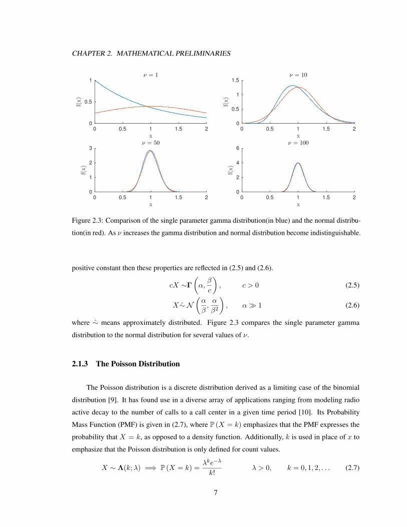
Figure 2.3: Comparison of the single parameter gamma distribution(in blue) and the normal distribu-
tion(in red). As ν increases the gamma distribution and normal distribution become indistinguishable.
positive constant then these properties are reflected in (2.5) and (2.6).
cX ∼Γ
(α,β
c
), c > 0 (2.5)
X∼ N(α
β,α
β2
), α� 1 (2.6)
where ∼ means approximately distributed. Figure 2.3 compares the single parameter gamma
distribution to the normal distribution for several values of ν.
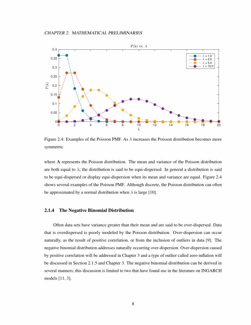
2.1.3 The Poisson Distribution
The Poisson distribution is a discrete distribution derived as a limiting case of the binomial
distribution [9]. It has found use in a diverse array of applications ranging from modeling radio
active decay to the number of calls to a call center in a given time period [10]. Its Probability
Mass Function (PMF) is given in (2.7), where P (X = k) emphasizes that the PMF expresses the
probability that X = k, as opposed to a density function. Additionally, k is used in place of x to
emphasize that the Poisson distribution is only defined for count values.
X ∼ Λ(k;λ) =⇒ P (X = k) =λke−λ
k!λ > 0, k = 0, 1, 2, . . . (2.7)
7
CHAPTER 2. MATHEMATICAL PRELIMINARIES
0 2 4 6 8 10 12 14 16 18 20
k
0
0.05
0.1
0.15
0.2
0.25
0.3
0.35
0.4P(k)
P(k) vs. λ
λ = 1.0
λ = 2.0
λ = 5.0
λ = 10.0
Figure 2.4: Examples of the Poisson PMF. As λ increases the Poisson distribution becomes more
symmetric
where Λ represents the Poisson distribution. The mean and variance of the Poisson distribution
are both equal to λ; the distribution is said to be equi-dispersed. In general a distribution is said
to be equi-dispersed or display equi-dispersion when its mean and variance are equal. Figure 2.4
shows several examples of the Poisson PMF. Although discrete, the Poisson distribution can often
be approximated by a normal distribution when λ is large [10].
2.1.4 The Negative Binomial Distribution
Often data sets have variance greater than their mean and are said to be over-dispersed. Data
that is overdispersed is poorly modeled by the Poisson distribution. Over-dispersion can occur
naturally, as the result of positive correlation, or from the inclusion of outliers in data [9]. The
negative binomial distribution addresses naturally occurring over-dispersion. Over-dispersion caused
by positive correlation will be addressed in Chapter 3 and a type of outlier called zero-inflation will
be discussed in Section 2.1.5 and Chapter 3. The negative binomial distribution can be derived in
several manners; this discussion is limited to two that have found use in the literature on INGARCH
models [11, 3].
8

CHAPTER 2. MATHEMATICAL PRELIMINARIES
In the first method the negative binomial distribution is viewed as a generalization of the
binomial distribution. Whereas the binomial distribution models the number of successes in n
Bernoulli trials, the negative binomial distribution models the number of successful Bernoulli trials
until r failures occur. Given r and the probability of a successful trial p the PMF of the negative
binomial distribution (referred to in the case as the NBB distribution) is
X ∼ NBB(k; r, p) =⇒ P (X = k) =
(k + r − 1
k
)pk (1− p)r (2.8)
k = 0, 1, 2, . . . , r = 0, 1, 2, . . . , 0 < p < 1
where(nk
)= n!
k!(n−k)! is the binomial coefficient and gives the number of ways to possibly choosek
trials from n when order does not matter. (2.8) is explained by observing that by definition there will
be k successes, each having probability p of occurring, r failures each with probability (1− p) of
occurring, and the k successes are chosen from k + r − 1 trials since the last trial is always a failure.
If factorial is replaced by the gamma function in the binomial coefficient then the distribution can be
generalized to allow r to be any real number greater than 0.
The second parameterization of the negative binomial distribution arises as the mixture of a
Poisson random variable and a gamma random variable. That is, given the Poisson rate parameter
λ = µ and the single parameter gamma distributed random variable Y then
P (X = k|Y = y) = Λ(k;µy) Y ∼ Γ(y; ν) (2.9)
and X is a negative binomial random variables with PMF
X ∼ NB2(k;µ, ν) =⇒ P (X = k) =Γ (k + ν)
Γ (ν) Γ (k + 1)
(ν
ν + µ
)ν ( µ
ν + µ
)k(2.10)
k = 0, 1, 2, . . . , µ > 0, ν > 0
A proof can be found in [9]. Using the law of iterated expectations, which states that
E [X] = E [E [X|Y ]] (2.11)
and the law of total variance which similarly says that
VAR [X] = VAR [E [X|Y ]] + E [VAR [X|Y ]] (2.12)
yields
E [X] = E [E [X|Y ]] = E [µY ] = µ (2.13)
9

CHAPTER 2. MATHEMATICAL PRELIMINARIES
0 5 10 15 20
k
0
0.05
0.1
0.15
0.2
0.25P
(k)
(a)
ν = 0.5
ν = 1.0
ν = 5.0
ν = 25.0
ν = 100.0
0 5 10 15 20
k
0
0.1
0.2
0.3
0.4
0.5
0.6
0.7
P(k
)
(b)
µ = 0.5
µ = 1.0
µ = 2.0
µ = 5.0
µ = 10.0
Figure 2.5: Examples of the Negative Binomial PMF. In (a) µ is held constant at 10 while ν is
changed. In (b) ν is held constant at 5 while µ is changed.
and
VX = E [VAR [X|Y ]] + VAR [E [X|Y ]] = E [µY ] + VAR [µY ] = µ+µ2
ν(2.14)
Since µ controls the mean of the distribution and ν controls the dispersion they are referred to as the
mean and dispersion parameters, respectively. The second parameterization, referred to as the NB2
distribution, is the preferred negative binomial distribution in the rest of this work. Figure 2.5 shows
examples of the NB2 distribution for different values of ν and µ.
2.1.5 Zero-Inflated Distributions
Another cause of over-dispersion in count time series is anomalous values. When there is an
excessive amount of zeros in a data set it is said to be zero-inflated. One way to model such cases
is through the use of zero-inflated distributions. To describe zero-inflated distributions let Z be a
Bernoulli random variable with probability of failure p0 (i.e., Z = 0), Y be a random variable of
arbitrary distribution, and let
X = Y Z (2.15)
Then X has a zero-inflated distribution with an underlying distribution equivalent to that of Y . The
term zero-inflated describes how X always equals 0 when Z = 0 but follows the same distribution
as Y when Z = 1. This creates an excess of zeros equal in probability to p0, which is referred to as
10

CHAPTER 2. MATHEMATICAL PRELIMINARIES
the zero-inflation parameter. More specifically
P (X = k; p0, Y ) =
p0 + (1− p0)P (Y = 0) k = 0
(1− p0)P (Y = k) k = 1, 2, 3, . . .(2.16)
Since Y and Z are independent
E [X] = E [Y ]E [Z] = (1− p0)µY (2.17)
and using (2.12)
VY = E [VAR [X|Y,Z]] + VAR [E [X|Y,Z]]
= p0VY + p0 ((1− p0)µY )2 + (1− p0) (p0µY )2
= (1− p0)(p0µ
2Y + VY
)(2.18)
This work focuses on the zero-inflated distributions with either an underlying Poisson or NB2
distribution, referred to as the ZIP and ZINB2, respectively. In this work we let
X ∼ Λ0(k;λ, p0)
X ∼ ZINB20(k;µ, ν, p0)
represent thatX is ZIP or ZINB2 distributed respectively. Applying (2.17) and (2.18) the mean and
variance of the ZIP distribution are
E [Λ0] = (1− p0)λ VAR [Λ0] = (1− p0)λ (1 + p0λ) (2.19)
and equivalently for the ZINB2 distribution
E [ZINB20] = (1− p0)µ VAR [ZINB20] = (1− p0)
(µ+
µ2
ν+ p0µ
2
)(2.20)
Figure 2.6 shows several examples of the ZIP and ZINB2 distributions.
11

CHAPTER 2. MATHEMATICAL PRELIMINARIES
0 5 10 15 20
k
0
0.05
0.1
0.15
0.2
0.25
P(k)
(a)
p0 = 0.00
p0 = 0.15
p0 = 0.25
0 5 10 15 200
0.05
0.1
0.15
0.2
0.25
(b)
p0 = 0.00
p0 = 0.15
p0 = 0.25
Figure 2.6: The ZIP(a) and ZINB2(b) PMFs as a function of p0. The solid lines for µ = λ = 5 and
the dashed lines are for µ = λ = 10. For the ZINB2 distribution ν = 5.
2.2 Time Series
This section gives a brief review of mathematical concepts pertinent to time series analysis. It
also serves the purpose of introducing the time series notation used through out the rest of this work.
A time series X can be viewed as a series of random variables sequential in time, such as (2.21).
X , {X1, X2, . . . Xn, . . .} (2.21)
For analysis of time series to be meaningful there is often some assumption of stationarity. Strict
stationarity refers to the invariance of all joint distributions of the time series with respect to all time.
This framework is extremely limiting therefore typically relaxed forms of stationarity are considered.
Instead we often assume second-order stationarity meaning
E [Xn] = µX ∀ n (2.22)
E [XnXn+k] = RX(k) ∀ n, k (2.23)
RX(k), referred to as the auto-correlation, is a measure of similarity between values separated k
steps in time. Similarly CX(k) is called the auto-covariance and is defined as
CX(k) = E [XnXn+k]− E [Xn]E [Xn+k] = RX(k)− µ2X (2.24)
12
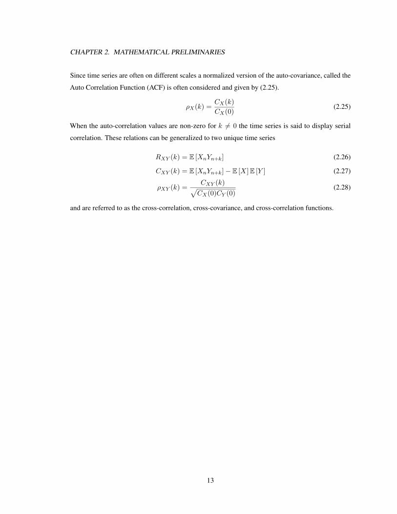
CHAPTER 2. MATHEMATICAL PRELIMINARIES
Since time series are often on different scales a normalized version of the auto-covariance, called the
Auto Correlation Function (ACF) is often considered and given by (2.25).
ρX(k) =CX(k)
CX(0)(2.25)
When the auto-correlation values are non-zero for k 6= 0 the time series is said to display serial
correlation. These relations can be generalized to two unique time series
RXY (k) = E [XnYn+k] (2.26)
CXY (k) = E [XnYn+k]− E [X]E [Y ] (2.27)
ρXY (k) =CXY (k)√CX(0)CY (0)
(2.28)
and are referred to as the cross-correlation, cross-covariance, and cross-correlation functions.
13
Chapter 3
Linear and Log-Linear Count Time
Series Models
Many time series models have been developed to account for serial correlation. Perhaps the most
well known is the ARMA family of models. ARMA models are used to describe continuous data and
are discussed briefly in Section 3.1. Recent work in the area of time series has led to the development
of INGARCH models for count data [6, 5], which are the focus of this chapter. Section 3.2 introduces
the linear model and develops results that, under mild conditions, are independent of the conditional
distribution. Sections 3.3 and 3.4 specialize these results for the Poisson and NB2 distributions. Next,
Section 3.5 develops similar results for zero-inflated models. In Sections 3.6 and 3.7 we specialize
these results for the ZIP and ZINB2 distributions. Last, in Section 3.8 we provide a brief discussion
of log-linear INGARCH models.
3.1 Auto-Regressive Moving-Average Models
ARMA models are a ubiquitous time series model that have been used to model many real
world phenomenon ranging from stock prices to the output of chemical processes [4]. ARMA
models traditionally represent continuous time series, but due to their mature nature as well as the
central limit theorem have been applied to count time series as well. Although the ARMA model
14
CHAPTER 3. LINEAR AND LOG-LINEAR COUNT TIME SERIES MODELS
is not specifically suited for the analysis of count time series understanding them greatly facilitates
comprehension of the linear INGARCH model.
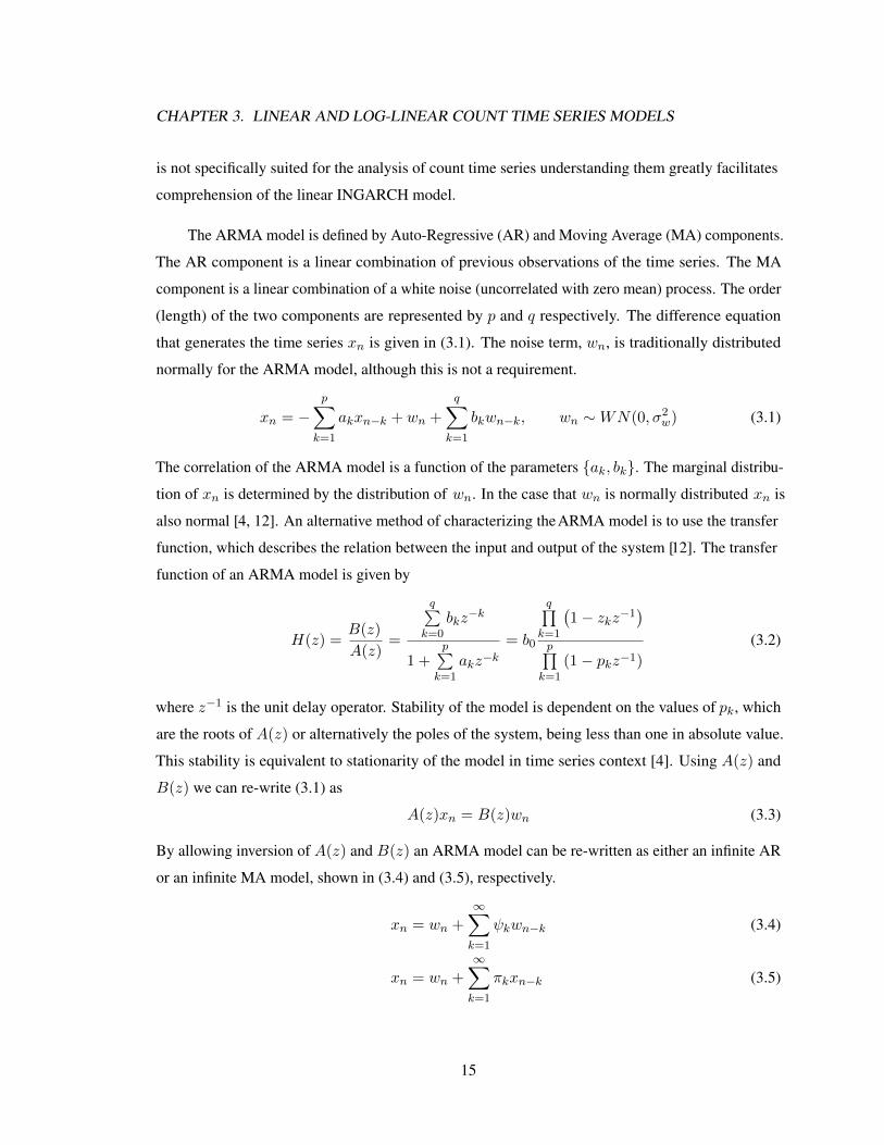
The ARMA model is defined by Auto-Regressive (AR) and Moving Average (MA) components.
The AR component is a linear combination of previous observations of the time series. The MA
component is a linear combination of a white noise (uncorrelated with zero mean) process. The order
(length) of the two components are represented by p and q respectively. The difference equation
that generates the time series xn is given in (3.1). The noise term, wn, is traditionally distributed
normally for the ARMA model, although this is not a requirement.
xn = −p∑
k=1
akxn−k + wn +
q∑k=1
bkwn−k, wn ∼WN(0, σ2w) (3.1)
The correlation of the ARMA model is a function of the parameters {ak, bk}. The marginal distribu-
tion of xn is determined by the distribution of wn. In the case that wn is normally distributed xn is
also normal [4, 12]. An alternative method of characterizing theARMA model is to use the transfer
function, which describes the relation between the input and output of the system [12]. The transfer
function of an ARMA model is given by
H(z) =B(z)
A(z)=
q∑k=0
bkz−k
1 +p∑
k=1
akz−k= b0
q∏k=1
(1− zkz−1
)p∏
k=1
(1− pkz−1)
(3.2)
where z−1 is the unit delay operator. Stability of the model is dependent on the values of pk, which
are the roots of A(z) or alternatively the poles of the system, being less than one in absolute value.
This stability is equivalent to stationarity of the model in time series context [4]. Using A(z) and
B(z) we can re-write (3.1) as
A(z)xn = B(z)wn (3.3)
By allowing inversion of A(z) and B(z) an ARMA model can be re-written as either an infinite AR
or an infinite MA model, shown in (3.4) and (3.5), respectively.
xn = wn +∞∑k=1
ψkwn−k (3.4)
xn = wn +∞∑k=1
πkxn−k (3.5)
15

CHAPTER 3. LINEAR AND LOG-LINEAR COUNT TIME SERIES MODELS
The individual coefficients πk and ψk are found by expanding (3.6) and (3.7) and equating like terms.
Π(z) = B(z)−1A(z) (3.6)
Ψ(z) = A(z)−1B(z) (3.7)
The infinite MA model is particularly useful for analysis as it expresses the model as a sum of
uncorrelated components.
3.2 Linear Count Models
This section develops the linear INGARCH model. Throughout the rest of this chapter the term
INGARCH is omitted for notational convenience when its absence does not affect understanding.
These models create serial correlation by conditioning the mean of the random variableXn on all past
information In−1 = {xn−1, xn−2, . . . }, under which the distribution of Xn is known to be a count
distribution parameterized by its mean. This conditional distribution, denoted D when the specific
distribution is arbitrary, is typically Poisson,NB2, ZIP, or ZINB2. The conditional distribution may
have any number of additional parameters that are constant with time. The conditional mean at time
n, denoted λn, is a function of past values of itself as well as past values of xn−k. For the linear
model, whose structure is given in (3.8) and (3.9), λn is a linear combination of xn−k and λn−k.
Xn ∼ D (λn(θ)|In−1) (3.8)
λn(θ) = E [Xn|In−1] = d+
p∑k=1
akxn−k +
q∑k=1
bkλn−k (3.9)
d > 0, 0 ≤ ak, bk < 1, 1 >
p∑k=1
ak +
q∑k=1
bk (3.10)
In (3.8) and (3.9) θ represents the set of model parameters {d, ak, bk}, p denotes the number of ak
terms in (3.9), and q denotes the number of bk terms in (3.9). Due to this similarity linear models
with only ak terms are referred to as AR models. Similar to ARMA models the linear models are
specified by their order (p,q). The (1,0) and (1,1) models are the most prevalent in the literature
as their analysis is straight-forward and they seem to be the most applicable to real-world data.
Specifically, models with feedback of λn have been found to perform better than higher order AR
models, even when the true model is a higher order AR model [7].
16

CHAPTER 3. LINEAR AND LOG-LINEAR COUNT TIME SERIES MODELS
Equation (3.10) ensures that λn is greater than zero regardless of the values ofxn−k and λn−k,
an inherent requirement of count distributions. Additionally, the constrained sum ensures first-order
stationarity of the linear model. we can see this by first assuming first-order stationarity of the linear
model. Under this assumption, upon expectation (3.9) becomes
E [λn(θ)] = E [E [Xn|In−1]]
= E
[d+
p∑k=1
akxn−k +
q∑k=1
bkλn−k
]
µΛ = d+
p∑k=1
akµX +
q∑k=1
bkµΛ (3.11)
However we know that µX = µΛ therefore (3.11) becomes
µX = d+
p∑k=1
akµX +
q∑k=1
bkµX (3.12)
Solving (3.12) for µX yields
µX =d
1−∑p
k=1 ak −∑q
k=1 bk(3.13)
where µX is the unconditional mean ofXn. Since the mean of any count distribution must be positive
(3.13) is only valid when the constraints of (3.10) are satisfied. Unlike ARMA models stationarity of
the linear model is dependent on {ak, bk} as opposed to just {ak}. Both terms are still important in
specifying the correlation of the models, however.
The serial correlation of the linear model can be derived without specifying D and instead
considering the error terms of the model. Following [7] let
En , Xn − Λn (3.14)
en , xn − λn (3.15)
If D is either Poisson or NB2 then using the law of iterated expectations
RE(k) = CE(k) = E [EnEn+k] = E [EnE [En+k|Dn+k−1]] = 0 (3.16)
showing that En is a white noise process [13]. Using En
CΛE(0) = 0 (3.17)
CXE(0) = E[X2n
]− E [XnΛn] (3.18)
CXΛ(0) = E [XnΛn]− µXµΛ (3.19)
17

CHAPTER 3. LINEAR AND LOG-LINEAR COUNT TIME SERIES MODELS
Additionally Λn and En being uncorrelated implies that
E [XnΛn] = E[Λ2n
](3.20)
E[X2n
]= E
[Λ2n
]+ E
[E2n
](3.21)
and that the variance of Xn can be written in a decoupled manner
VX = VΛ + VE (3.22)
Substitution of (3.20) and (3.21) into (3.18) and (3.19) yields
CΛE(0) = 0 (3.23)
CXE(0) = VE (3.24)
CXΛ(0) = VΛ (3.25)
These results are used in Appendix A to derive the serial correlation of the (1,0) and (1,1) models,
which have been previously derived in [6, 1]. The results are given in Table 3.1 and show that the
ACFs of both (1,0) and (1,1)models are independent of the conditional distribution. The variances of
the models however, are not.
While the approach taken in Appendix A is instructive in understanding the underlying process,it is intractable in deriving results for higher order models. Theorem 1 of [8] provides recursiveequations, given by (3.26), that can be used to find the auto-covariances of Xn and Λn as well astheir cross-covariance. These results only depend on the assumption that µX = µΛ and thus hold forthe NB2 model as well as the Poisson model.
CX(k) =
p∑i=1
aiCX(k)[|k − i|] +
min(k−1,q)∑i=1
biCX(k − i) +
q∑i=k
biCΛ(i− k) k ≥ 1 (3.26a)
CΛ(k) =
min(k,p)∑i=1
aiCΛ(k)[|k − i|] +
p∑i=k+1
aiCX(k)[k − i] +
q∑i=1
biCΛ(k)[|k − i|] k ≥ 0 (3.26b)
CXΛ(k) = CΛΛ(k), k ≥ 0, CXΛ(k) = CXX(k), k < 0 (3.26c)
Unfortunately, these results are also difficult to extend to higher order models.
18

CHAPTER 3. LINEAR AND LOG-LINEAR COUNT TIME SERIES MODELS
Table 3.1: Covariance and ACF of the linear (1,0) and (1,1) models. Under the assumption of
uncorrelated errors the ACF is independent of the conditional distribution.
Value (1, 0) (1, 1)
VXVE
1−a2 VE1−(a+b)2+a2
1−(a+b)2
VΛa2VE1−a2
a2VE1−(a+b)2
CX(k) akVX VXa(1−b(a+b))(a+b)k−1
1−(a+b)2+a2
ρX(k) ak a(1−b(a+b))(a+b)k−1
1−(a+b)2+a2
CΛ(k) akVΛ (a+ b)k VΛ
ρΛ(k) ak (a+ b)k
CΛX(k) k > 0 akVX VXa(1−b(a+b))(a+b)k−1
1−(a+b)2+a2(a+b)k−1
CΛX(k) k ≤ 0 a|k|+2VX VXa2(a+b)k
1−(a+b)2+a2
ρΛX(k) k > 0 ak−1 (a+b)k−1(1−b(a+b))√1−b2−2ab
ρΛX(k) k ≤ 0 a|k|+1 a(a+b)k√1−b2−2ab
An alternative approach is to follow the work of [13] and re-write (3.9) as
xn = d+
max(p,q)∑k=1
(ak + bk)xn−k + en −q∑
k=1
bken−k (3.27)
Letting αk = −(ak + bk) and βk = −bk (3.27) becomes
xn = d−max(p,q)∑k=1
αkxn−k + en +
q∑k=1
βken−k (3.28)
and is identical to (3.1) except for the addition of d. This only affects the mean of the model however,
and does not affect the correlation of the model. Figures 3.1 and 3.2 show the parameter space of the
linear (1,1) model in (a, b), (α, β), and (ρ1, ρ2) space. Similarly, if εn = a1en−1 and κk = aka1
then
19

CHAPTER 3. LINEAR AND LOG-LINEAR COUNT TIME SERIES MODELS
λn can be re-written as
λn = d−max(p,q)∑k=1
αkλn−k + εn +
p−1∑k=1
κkεn−k (3.29)
Since εn is a scaled and time-delayed version of en it is a white noise process and λn can also be
written as an ARMA model. Both xn and λn can then be re-written as infinite MA processes, given
by (3.30) and (3.31).
xn = µX + en +∞∑i=1
ψ(x)k en−k (3.30)
λn = µΛ + εn +∞∑i=1
ψ(λ)k εn−k (3.31)
The unconditional variance of both Xn and Λn are then found to be
VX =
(1 +
∞∑k=1
ψ2k
)VE (3.32)
VΛ =
( ∞∑k=1
ψ2k
)VE (3.33)
This result is efficacious in deriving several new results for the linear model.
20

CHAPTER 3. LINEAR AND LOG-LINEAR COUNT TIME SERIES MODELS
Figure 3.1: Admissible region of parameter values for the linear (1,1) model. The left hand plot
shows the region in (ak, bk) space and the right hand plot shows the region in (α,β) space.
Figure 3.2: Admissible region of parameter values for the linear INGARCH(1,1) model in (ρ1,ρ2)
space.
21

CHAPTER 3. LINEAR AND LOG-LINEAR COUNT TIME SERIES MODELS
3.3 The Poisson Linear Model
The simplest linear model is the Poisson model, which has been previously studied in [6, 1, 5].
Many of the results in this section echo those found in the literature mentioned. One result that is
absent however is the marginal distribution of the Poisson model, for which a closed form solution
does not exist. The main result of this section is to provide a simple approximation for the marginal
distribution of the (1,0) and (1,1) models.
Before the marginal distribution is discussed, it is important we understand the correlation of
the Poisson model. Using the law of total variance and conditioning on In−1 shows that
VAR [En] = VAR [E [En|In−1]] + E [VAR [En|In−1]] = 0 + E [Λn] = E [Xn] (3.34)
Substitution of (3.34) into (3.22) shows that for the Poisson model
VX = VΛ + µX (3.35)
As expected introducing correlation into the time series produces over-dispersion. The results of
applying (3.34) to Table 3.1 are given in Table 3.2.
Figure 3.3 shows several examples of the Poisson (1,0) model with differing θ. The parameters
were chosen so that the unconditional mean of the observed time series are the same in Figures
3.3a, 3.3b, and 3.3c. As a increases while holding µX constant the correlation of Xn becomes
more clear. Similar to the ARMA model both xn and λn closely track xn−1, creating the peaks and
values observed in Figures 3.3c and 3.3d. Additionally, increased correlation inflates the tails of
the marginal distribution as large values of xn become more common due to the correlation. The
parameter d was chosen in Figure 3.3d to demonstrate the effect of increasing the mean while holding
a constant. Both Figure 3.3c and Figure 3.3d exhibit similar shapes but, despite the equal correlation
coefficients, increased variance causes more jaggedness in Figure 3.3d.
Figure 3.4 shows similar results for the (1,1) model. Comparing the observed ACFs in Figures
3.4a and 3.4b to those in Figures 3.4c and 3.4d demonstrates that, as noted in [13], inclusion of mean
regressors causes the ACF to decay at a slower rate. This produces elongated trends in Xn. This
helps explain why (1,1) models have been observed to perform better than higher order AR models,
as both yield similar effects but the (1,1) model is more parsimonious.
22

CHAPTER 3. LINEAR AND LOG-LINEAR COUNT TIME SERIES MODELS
(a) d = 8, a = 0.2.
0 10 20 30 40 50 60 70 80 90 100
5
10
15
20
25
0 5 10 15 20 250
0.05
0.1
0.15
Marginal
NB2
0 5 10 15 20
k
0
0.5
1
ρX
X(k
)
Obs.
Exp.
0 5 10 15 20
k
0
0.5
1
ρλλ(k
)
-10 -5 0 5 10
k
0
0.5
1
ρXλ(k
)
(b) d = 5, a = 0.5.
0 10 20 30 40 50 60 70 80 90 100
5
10
15
20
0 5 10 15 20 250
0.05
0.1
0.15
Marginal
NB2
0 5 10 15 20
k
0
0.5
1
ρX
X(k
)
Obs.
Exp.
0 5 10 15 20
k
0
0.5
1
ρλλ(k
)
-10 -5 0 5 10
k
0
0.5
1
ρXλ(k
)
(c) d = 2, a = 0.8.
0 10 20 30 40 50 60 70 80 90 100
5
10
15
20
25
0 5 10 15 20 250
0.05
0.1
Marginal
NB2
0 5 10 15 20
k
0
0.5
1
ρX
X(k
)
Obs.
Exp.
0 5 10 15 20
k
0
0.5
1
ρλλ(k
)
-10 -5 0 5 10
k
0
0.5
1
ρXλ(k
)
(d) d = 5, a = 0.8.
0 10 20 30 40 50 60 70 80 90 10010
20
30
40
0 10 20 30 40 500
0.02
0.04
0.06
Marginal
NB2
0 5 10 15 20
k
0
0.5
1
ρX
X(k
)
Obs.
Exp.
0 5 10 15 20
k
0
0.5
1
ρλλ(k
)
-10 -5 0 5 10
k
0
0.5
1
ρXλ(k
)
Figure 3.3: Examples of the Poisson (1,0) model. Each plot shows from top right clockwise:
xn in blue and λn in red; The expected and observed ACF of Xn; The expected and observed
cross-correlation function of Xn and Λn; the expected and observed ACF of Λn; and the marginal
distribution of a time series of length 1 million and a fitted NB2 distribution.
23

CHAPTER 3. LINEAR AND LOG-LINEAR COUNT TIME SERIES MODELS
(a) d = 1, a = 0.2, b = 0.7.
0 10 20 30 40 50 60 70 80 90 100
5
10
15
0 5 10 15 20 25 300
0.05
0.1
0.15
Marginal
NB2
0 5 10 15 20
k
0
0.5
1
ρX
X(k
)
Obs.
Exp.
0 5 10 15 20
k
0
0.5
1
ρλλ(k
)
-10 -5 0 5 10
k
0
0.5
1
ρXλ(k
)
(b) d = 1, a = 0.5, b = 0.4.
0 10 20 30 40 50 60 70 80 90 100
5
10
15
20
25
0 5 10 15 20 25 300
0.05
0.1
Marginal
NB2
0 5 10 15 20
k
0
0.5
1
ρX
X(k
)
Obs.
Exp.
0 5 10 15 20
k
0
0.5
1
ρλλ(k
)
-10 -5 0 5 10
k
0
0.5
1
ρXλ(k
)
(c) d = 1, a = 0.8, b = 0.1.
0 10 20 30 40 50 60 70 80 90 100
0
20
40
0 5 10 15 20 25 300
0.05
0.1
Marginal
NB2
0 5 10 15 20
k
0
0.5
1
ρX
X(k
)
Obs.
Exp.
0 5 10 15 20
k
0
0.5
1
ρλλ(k
)
-10 -5 0 5 10
k
0
0.5
1
ρXλ(k
)
(d) d = 4, a = 0.3, b = 0.3.
0 10 20 30 40 50 60 70 80 90 100
5
10
15
20
0 5 10 15 20 25 300
0.05
0.1
0.15
Marginal
NB2
0 5 10 15 20
k
0
0.5
1
ρX
X(k
)
Obs.
Exp.
0 5 10 15 20
k
0
0.5
1
ρλλ(k
)
-10 -5 0 5 10
k
0
0.5
1
ρXλ(k
)
Figure 3.4: Examples of the Poisson (1,1) model. Each plot shows from top right clockwise: xn in red
and λn in blue; The expected and observed ACF of Xn; The expected and observed cross-correlation
function of Xn and Λn; the expected and observed ACF of Λn; and the marginal distribution of a
time series of length 1 million and a fitted NB2 distribution.
24

CHAPTER 3. LINEAR AND LOG-LINEAR COUNT TIME SERIES MODELS
Table 3.2: Dynamics of the Poisson (1,0) and (1,1) linear models.
Value (1, 0) (1, 1)
VXµX
1−a2 µX1−(a+b)2+a2
1−(a+b)2
VΛa2µΛ
1−a2a2µX
1−(a+b)2
CX(k) ak µX1−a2 µX
a(1−b(a+b))(a+b)k−1
1−(a+b)2
ρX(k) ak a(1−b(a+b))(a+b)k−1
1−(a+b)2+a2
CΛ(k) ak µΛ
1−a2 µΛa2(a+b)k
1−(a+b)2
ρΛ(k) ak (a+ b)k
CΛX(k) k > 0 ak µX1−a2 µX
a(1−b(a+b))(a+b)k−1
1−(a+b)2
CΛX(k) k ≤ 0 a|k|+2 µX1−a2 µX
a2(a+b)k
1−(a+b)2
ρΛX(k) k > 0 ak−1 (1−b(a+b))(a+b)k−1
√1−b2−2ab
ρΛX(k) k ≤ 0 a|k|+1 a(a+b)k√1−b2−2ab
The marginal distribution of the Poisson model does not have a closed form. In [8], the author
found higher order moments of the (1,0) model via the moment generating function, but these
results do not appear to be adaptable to higher order models or models with different conditional
distributions. We show that under certain conditions approximating the marginal distribution of the
Poisson linear model via the NB2 distribution is viable for certain applications. To begin assume that
en can be approximated by the normal distribution. Next, using (3.15) and (3.30) we re-write λn as
λn = µΛ + a
∞∑i=1
(a+ b)i−1 en−i (3.36)
Under the assumption that en∼N (0, µX) (3.36) shows that λn is the sum of uncorrelated normal
random variables and thus also normally distributed with mean µΛ and variance VΛ. Next, we use
the gamma-normal approximation and solve for k and θ to find
k =d (1 + (a+ b))
a2θ =
a2
1− (a+ b)2
25

CHAPTER 3. LINEAR AND LOG-LINEAR COUNT TIME SERIES MODELS
Using the scaling property, Λn can be described as a single parameter gamma distribution
Λn∼µΛΓ
(ν =
d (1 + (a+ b))
a2
)(3.37)
Finally, from the definition of the NB2 distribution, (3.37) implies that Xn is NB2 distributed
Xn∼NB2
(µX ,
d (1 + (a+ b))
a2
)(3.38)
The most important assumption in this approximation is that ν is large. Since ν is directly
proportional to d and b we expect this approximation to perform better for larger values of d and b.
This result is logical because as d and b increase each realization of Xn becomes better approximated
by the normal distribution and therefore En does as well. Conversely, ν is inversely proportional to a
so we expected better results as a decreases. As a approaches zero ν approaches∞ and the marginal
distribution becomes IID Poisson and the conditional distribution also becomes IID Poisson. This is
expected since when a = 0 there is no feedback meaningλn does not change (once steady state has
been reached) and the marginal and conditional distributions are identical.
Figures 3.5 and 3.6 show the normalized error of the marginal distribution compared to the
approximate NB2 distribution for the (1,0) and (1,1) models. The true marginal distribution was
approximated by generating a time series of 10 million points. The approximation performed well
inside the 99% confidence bound, especially near the center, where we observe less than 2% error.
Also, as expected, as d and b increased the approximation improved while increasing a degraded
performance. Unfortunately because this is only an approximation and we cannot use it as a statistical
test. Additionally, it relies on the time series being too long for practical use in most applications.
One possible application is for horizon forecasts.
To analyze higher order models in a similar manner the Poisson model must be transformed into
an ARMA model. (3.30) and (3.31) can be used to find the unconditional variance of Xn and Λn
VX =
(1 +
∞∑k=1
ψ2k
)µX (3.39)
VΛ =
( ∞∑k=1
ψ2k
)µX (3.40)
26

CHAPTER 3. LINEAR AND LOG-LINEAR COUNT TIME SERIES MODELS
Following the approach laid out earlier we arrive at (3.41) and (3.42).
Λn ∼ µXΓ
(µX∑∞
i=1 ψken−k
)(3.41)
Xn ∼ NB2
(µX ,
µX∑∞i=1 ψken−k
)(3.42)
Again we expect this approximation to hold well for larger d and b.
27

CHAPTER 3. LINEAR AND LOG-LINEAR COUNT TIME SERIES MODELS
0 5 10 15
-0.1
-0.05
0
0.05
0.1
0 2 4 6 8 10 12 14 16 18
-0.1
-0.05
0
0.05
0.1
5 10 15 20 25
-0.1
-0.05
0
0.05
0.1
10 15 20 25 30 35 40 45 50
-0.1
-0.05
0
0.05
0.1
(a) d = 5
2 4 6 8 10 12 14 16 18 20 22 24
-0.1
-0.05
0
0.05
0.1
5 10 15 20 25 30
-0.1
-0.05
0
0.05
0.1
10 15 20 25 30 35 40
-0.1
-0.05
0
0.05
0.1
30 40 50 60 70 80
-0.1
-0.05
0
0.05
0.1
(b) d = 10
15 20 25 30 35 40
-0.1
-0.05
0
0.05
0.1
20 25 30 35 40 45 50
-0.1
-0.05
0
0.05
0.1
30 35 40 45 50 55 60 65 70 75
-0.1
-0.05
0
0.05
0.1
60 70 80 90 100 110 120 130 140
-0.1
-0.05
0
0.05
0.1
(c) d = 20
45 50 55 60 65 70 75 80 85
-0.1
-0.05
0
0.05
0.1
60 65 70 75 80 85 90 95 100 105 110
-0.1
-0.05
0
0.05
0.1
90 100 110 120 130 140 150 160
-0.1
-0.05
0
0.05
0.1
200 220 240 260 280 300 320
-0.1
-0.05
0
0.05
0.1
(d) d = 50
Figure 3.5: Normalized error of the observed PDF of the marginal distribution of the (1,0) Poisson
model distribution and the approximated marginal. The true marginal was generated by producing
time series of length 10 million. The blue and red lines represent the location of the 99% bounds
of the true and approximated bounds, respectively. For each set of plots, from top to bottom
a = {0.2, 0.4, 0.6, 0.8}.
28

CHAPTER 3. LINEAR AND LOG-LINEAR COUNT TIME SERIES MODELS
15 20 25 30 35 40
-0.1
-0.05
0
0.05
0.1
10 15 20 25 30 35 40
-0.1
-0.05
0
0.05
0.1
10 15 20 25 30 35 40 45
-0.1
-0.05
0
0.05
0.1
10 15 20 25 30 35 40 45
-0.1
-0.05
0
0.05
0.1
(a) d = 5
35 40 45 50 55 60 65 70
-0.1
-0.05
0
0.05
0.1
30 35 40 45 50 55 60 65 70
-0.1
-0.05
0
0.05
0.1
30 35 40 45 50 55 60 65 70 75
-0.1
-0.05
0
0.05
0.1
30 40 50 60 70 80
-0.1
-0.05
0
0.05
0.1
(b) d = 10
75 80 85 90 95 100 105 110 115 120 125
-0.1
-0.05
0
0.05
0.1
80 90 100 110 120 130
-0.1
-0.05
0
0.05
0.1
70 80 90 100 110 120 130
-0.1
-0.05
0
0.05
0.1
70 80 90 100 110 120 130 140
-0.1
-0.05
0
0.05
0.1
(c) d = 20
210 220 230 240 250 260 270 280 290
-0.1
-0.05
0
0.05
0.1
210 220 230 240 250 260 270 280 290
-0.1
-0.05
0
0.05
0.1
200 210 220 230 240 250 260 270 280 290 300
-0.1
-0.05
0
0.05
0.1
200 220 240 260 280 300
-0.1
-0.05
0
0.05
0.1
(d) d = 50
Figure 3.6: Normalized error of the observed PDF of the marginal distribution of the (1,1) Poisson
model distribution and the approximated marginal. The true marginal was generated by producing
time series of length 10 million. The blue and red lines represent the location of the 99% bounds
of the true and approximated bounds, respectively. For each set of plots, from top to bottom
a = {0.1, 0.3, 0.5, 0.7}, b = {0.1, 0.3, 0.5, 0.7}.
29

CHAPTER 3. LINEAR AND LOG-LINEAR COUNT TIME SERIES MODELS
3.4 The NB2 Linear Model
The natural extension of the Poisson model is the NB2 model. The negative binomial model
using the Negative Binomial (NBB) discussed briefly in Chapter 2 has been studied in some detail
in [11]. More recently, a similar analysis using the NB2 distribution was performed by [3] . One of
the benefits of using the NB2 distribution as opposed to the NBB distribution is that the region of
first order stationarity is independent of ν [11, 3]. Additionally, as previously shown, the ACF is also
independent of ν. This is noted in [3] as beneficial because it removes the need to check the value of
ν during parameter estimation. This warrants further investigation however, as even though the ACF
is independent of ν, existence of the variance is not.
Similar to the conditional Poisson, we calculate VE using the law of total variance
VAR [En] = VAR [E [En|In−1]] + E [VAR [En|In−1]] = 0 + E [Λn] +E[Λ2n
]ν
(3.43)
Upon substitution of E[Λ2n
]= E
[X2n
]+ VE into (3.43) we find
VE = µX +E[X2n
]− VE
ν(3.44)
Expanding E[X2n
]and solving for VE in terms of VX and µX yields
VE =VX + µ2
X + µXν
1 + ν(3.45)
Inserting this result into (3.22) and solving for Vx produces
VX = µX +µ2X
ν+
(1 + ν)
νVΛ (3.46)
Like the Poisson model, the introduction of correlation causes over dispersion of the marginal
distribution with respect to the conditional distribution. The NB2 model also exhibits greater
variance for given θ than the Poisson model, making it more appropriate for time series that exhibit
high variability. When ν approaches∞ the NB2 model reduces to the Poisson model, as expected.
Table 3.3 gives the correlation of the NB2 model where (3.45) has been substituted into Table 3.1.
Unlike the Poisson model, where the constraints for first order and second order stationarity
are identical, additional constraints must be imposed to ensure second order stationarity of theNB2
model. Table 3.3 shows that for the NB2 (1,0) model
ν >a2
1− a2(3.47)
30
CHAPTER 3. LINEAR AND LOG-LINEAR COUNT TIME SERIES MODELS
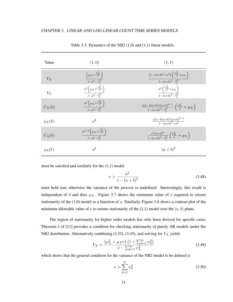
Table 3.3: Dynamics of the NB2 (1,0) and (1,1) linear models.
Value (1, 0) (1, 1)
VX
(µX+
µ2Xν
)1−a2−a2
ν
(1−(a+b)2+a2)(µ2Xν
+µX
)1−(a+b)2−a2
ν
VΛ
a2
(µX+
µ2Xν
)1−a2−a2
ν
a2
(µ2Xν
+µX
)1−(a+b)2−a2
ν
CX(k)ak
(µX+
µ2Xν
)1−a2−a2
ν
a(1−b(a+b))(a+b)k−1
1−(a+b)2−a2
ν
(µ2Xν + µX
)ρX(k) ak a(1−b(a+b))(a+b)k−1
1−(a+b)2+a2
CΛ(k)ak+2
(µX+
µ2Xν
)1−a2−a2
ν
a2(a+b)k
1−(a+b)2−a2
ν
(µ2Xν + µX
)ρΛ(k) ak (a+ b)k
must be satisfied and similarly for the (1,1) model
ν >a2
1− (a+ b)2 (3.48)
must hold true otherwise the variance of the process is undefined. Interestingly, this result is
independent of d and thus µX . Figure 3.7 shows the minimum value of ν required to ensure
stationarity of the (1,0) model as a function of a. Similarly, Figure 3.8 shows a contour plot of the
minimum allowable value of ν to ensure stationarity of the (1,1) model over the (a, b) plane.
The region of stationarity for higher order models has only been derived for specific cases.
Theorem 2 of [11] provides a condition for checking stationarity of purely AR models under the
NB2 distribution. Alternatively combining (3.32), (3.45), and solving for VX yields
VX =
(µ2X + µXν
) (1 +
∑∞k=1 ψ
2k
)ν −
∑∞k=1 ψ
2k
(3.49)
which shows that the general condition for the variance of the NB2 model to be defined is
ν >∞∑k=1
ψ2k (3.50)
31

CHAPTER 3. LINEAR AND LOG-LINEAR COUNT TIME SERIES MODELS
0 0.1 0.2 0.3 0.4 0.5 0.6 0.7 0.8 0.9 1
a
0
1
2
3
4
5
6
7
8
9
10ν
Figure 3.7: The minimum inverse dispersion parameter ν required for second-order stationarity, as a
function of a.
This result is important for model estimation to we can use it to ensure stationarity of the estimated
model.
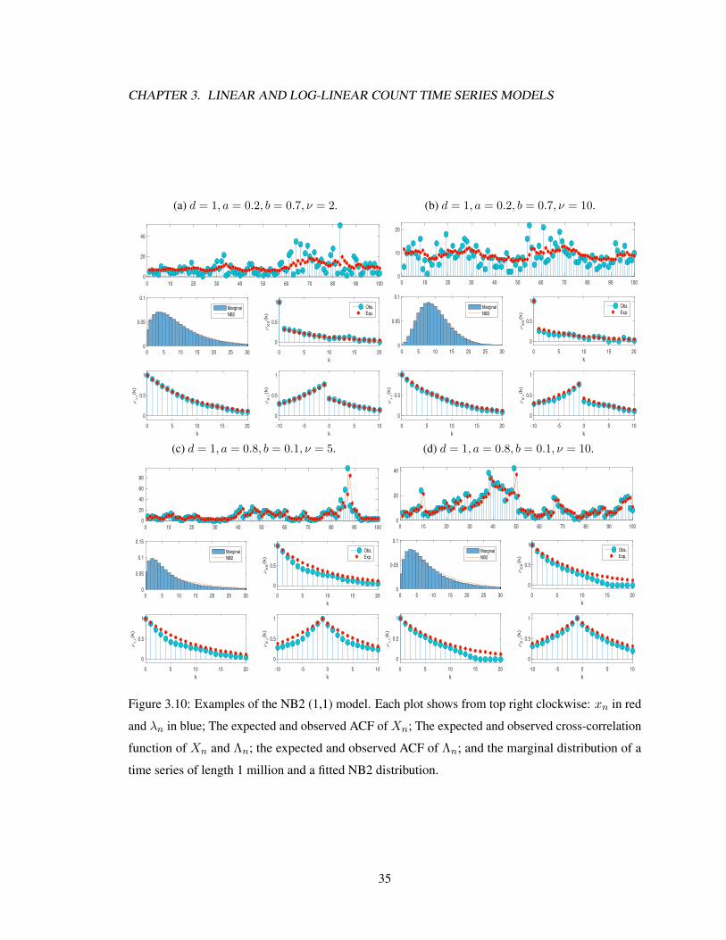
Figure 3.9 show several examples of the NB2 (1,0) model. The parameter set θ was chosen
to reflect the effects of ν on the model. As ν decreases the intensity and frequency of outliers
decreases as expected. This is reflected in the time series as well as the marginal distribution where
the over-dispersion compared to the best fit NB2 distribution is quite apparent in Figures 3.9a and
3.9b but is less so in Figures 3.9c and 3.9d. Figure 3.10 shows similar effects for the (1,1) model.
32

CHAPTER 3. LINEAR AND LOG-LINEAR COUNT TIME SERIES MODELS
Figure 3.8: The minimum inverse dispersion parameter ν required for second-order stationarity, as a
function of a and b.
33

CHAPTER 3. LINEAR AND LOG-LINEAR COUNT TIME SERIES MODELS
(a) d = 5, a = 0.5, ν = 1.
0 10 20 30 40 50 60 70 80 90 1000
20
40
60
0 10 20 30 400
0.05
0.1
0.15
Marginal
NB2
0 5 10 15 20
k
0
0.5
1
ρX
X(k
)
Obs.
Exp.
0 5 10 15 20
k
0
0.5
1
ρλλ(k
)
-10 -5 0 5 10
k
0
0.5
1
ρXλ(k
)
(b) d = 5, a = 0.5, ν = 2.
0 10 20 30 40 50 60 70 80 90 100
0
20
40
0 10 20 30 400
0.05
0.1
Marginal
NB2
0 5 10 15 20
k
0
0.5
1
ρX
X(k
)
Obs.
Exp.
0 5 10 15 20
k
0
0.5
1
ρλλ(k
)
-10 -5 0 5 10
k
0
0.5
1
ρXλ(k
)
(c) d = 5, a = 0.5, ν = 5.
0 10 20 30 40 50 60 70 80 90 1000
10
20
30
0 10 20 30 400
0.05
0.1
Marginal
NB2
0 5 10 15 20
k
0
0.5
1
ρX
X(k
)
Obs.
Exp.
0 5 10 15 20
k
0
0.5
1
ρλλ(k
)
-10 -5 0 5 10
k
0
0.5
1
ρXλ(k
)
(d) d = 5, a = 0.5, ν = 10.
0 10 20 30 40 50 60 70 80 90 1000
10
20
0 10 20 30 400
0.05
0.1
Marginal
NB2
0 5 10 15 20
k
0
0.5
1
ρX
X(k
)
Obs.
Exp.
0 5 10 15 20
k
0
0.5
1
ρλλ(k
)
-10 -5 0 5 10
k
0
0.5
1
ρXλ(k
)
Figure 3.9: Examples of the NB2 (1,0) model. Each plot shows from top right clockwise: xn in red
and λn in blue; The expected and observed ACF of Xn; The expected and observed cross-correlation
function of Xn and Λn; the expected and observed ACF of Λn; and the marginal distribution of a
time series of length 1 million and a fitted NB2 distribution.
34
CHAPTER 3. LINEAR AND LOG-LINEAR COUNT TIME SERIES MODELS
(a) d = 1, a = 0.2, b = 0.7, ν = 2.
0 10 20 30 40 50 60 70 80 90 100
0
20
40
0 5 10 15 20 25 300
0.05
0.1
Marginal
NB2
0 5 10 15 20
k
0
0.5
1
ρX
X(k
)
Obs.
Exp.
0 5 10 15 20
k
0
0.5
1
ρλλ(k
)
-10 -5 0 5 10
k
0
0.5
1
ρXλ(k
)
(b) d = 1, a = 0.2, b = 0.7, ν = 10.
0 10 20 30 40 50 60 70 80 90 1000
10
20
0 5 10 15 20 25 300
0.05
0.1
Marginal
NB2
0 5 10 15 20
k
0
0.5
1
ρX
X(k
)
Obs.
Exp.
0 5 10 15 20
k
0
0.5
1
ρλλ(k
)
-10 -5 0 5 10
k
0
0.5
1
ρXλ(k
)
(c) d = 1, a = 0.8, b = 0.1, ν = 5.
0 10 20 30 40 50 60 70 80 90 1000
20
40
60
80
0 5 10 15 20 25 300
0.05
0.1
0.15
Marginal
NB2
0 5 10 15 20
k
0
0.5
1
ρX
X(k
)
Obs.
Exp.
0 5 10 15 20
k
0
0.5
1
ρλλ(k
)
-10 -5 0 5 10
k
0
0.5
1
ρXλ(k
)
(d) d = 1, a = 0.8, b = 0.1, ν = 10.
0 10 20 30 40 50 60 70 80 90 1000
20
40
0 5 10 15 20 25 300
0.05
0.1
Marginal
NB2
0 5 10 15 20
k
0
0.5
1
ρX
X(k
)
Obs.
Exp.
0 5 10 15 20
k
0
0.5
1
ρλλ(k
)
-10 -5 0 5 10
k
0
0.5
1
ρXλ(k
)
Figure 3.10: Examples of the NB2 (1,1) model. Each plot shows from top right clockwise: xn in red
and λn in blue; The expected and observed ACF of Xn; The expected and observed cross-correlation
function of Xn and Λn; the expected and observed ACF of Λn; and the marginal distribution of a
time series of length 1 million and a fitted NB2 distribution.
35

CHAPTER 3. LINEAR AND LOG-LINEAR COUNT TIME SERIES MODELS
3.5 Zero-Inflated Linear Models
The zero-inflated linear model is an extension of the linear model. These models have been
studied in [14], where zero-inflated models were used to study arson data from the 13th police beat
in Pittsburgh, Pennsylvania. There are several differences between the zero-inflated model and the
regular model. First, by definition of zero-inflation
E [Xn|In−1] = (1− p0)λn (3.51)
Then, taking the expectation of (3.51) yields
µX = (1− p0)µΛ (3.52)
Plugging (3.52) into (3.12) and solving produces
µX =(1− p0) d
1−∑p
k=1 (1− p0) ak −∑q
k=1 bk(3.53)
From (3.53) we observe that the parameter space of the zero-inflated models have different constraints
than the linear models to ensure first-order stationarity. These constraints, given in (3.54), are more
relaxed than those of (3.10).
0 ≤ ak, bk < 1
p∑k=1
(1− p0) ak +
q∑k=1
bk < 1 0 ≤ p0 < 1 (3.54)
Additionally, in contrast to Section 3.2, Λn and En are no longer uncorrelated when the conditional
distribution is zero-inflated. This means that instead of being decoupled
VX = VΛ + VE + 2CΛE(0) (3.55)
To find the covariance between Λn and En let Z be an indicator random variable where Zt indicates
that Xn is zero-inflated and Zf indicates it is not. Using the law of total covariance, which states that
COV [X,Y ] = E [COV [X,Y |Z]] + COV [E [X|Z] ,E [X|Z]] (3.56)
yields
COV [Λn, En] = p0COV [Λn, En|Zt] + (1− p0) COV [Λn, En|Zf ]
+ p0 (E [E [Λn|Zt]E [En|Zt]]− E [E [Λn|Zt]]E [E [En|Zt]])
+ (1− p0) (E [E [Λn|Zf ]E [En|Zf ]]− E [E [Λn|Zf ]]E [E [En|Zf ]])
(3.57)
36

CHAPTER 3. LINEAR AND LOG-LINEAR COUNT TIME SERIES MODELS
When Z = Zf we observe that Xn is not zero-inflated and is thus uncorrelated with En. In this case
the second and fourth terms both equal zero. Additionally Z = Zt implies that En = −Λn, meaning
COV [Λn, En|Zt] = −VΛ and E [E [Λn|Zt]E [En|Zt]] = −µ2Λ. Substituting these values into (3.57)
and simplifying yields
COV [Λn, En] = −p0VΛ (3.58)
Using (3.15) to express VX in terms of VΛ and VE yields
VX = (1− 2p0)VΛ + VE (3.59)
Similarly
COV [Xn, En] = E[X2n
]− E [XnΛn]− E [Xn]E [Λn] (3.60)
COV [Xn,Λn] = E [XnΛn]− E [Xn]E [Λn] (3.61)
Expanding E[X2n
]shows that
E[X2n
]= E
[Λ2n
]− 2E [ΛnEn] + E
[E2n
](3.62)
Additionally (3.58) implies that
E [ΛnEn] = −p0E[Λ2n
](3.63)
E [XnΛn] = (1− p0)E[Λ2n
](3.64)
Using these results to simplify (3.60) and (3.61) yields
CΛE(0) = −p0VΛ (3.65)
CXE(0) = VX − (1− p0)VΛ (3.66)
CXΛ(0) = (1− p0)VΛ (3.67)
In Appendix A these results are used to derive the correlation of the zero-inflated (1,0) linear
model, which is given in Table 3.4. Compared to the linear models the correlation of the zero-inflated
models is not as strong for a given a. This result is expected as whenever zero-inflation occurs Xn is
independent of In−1.
37
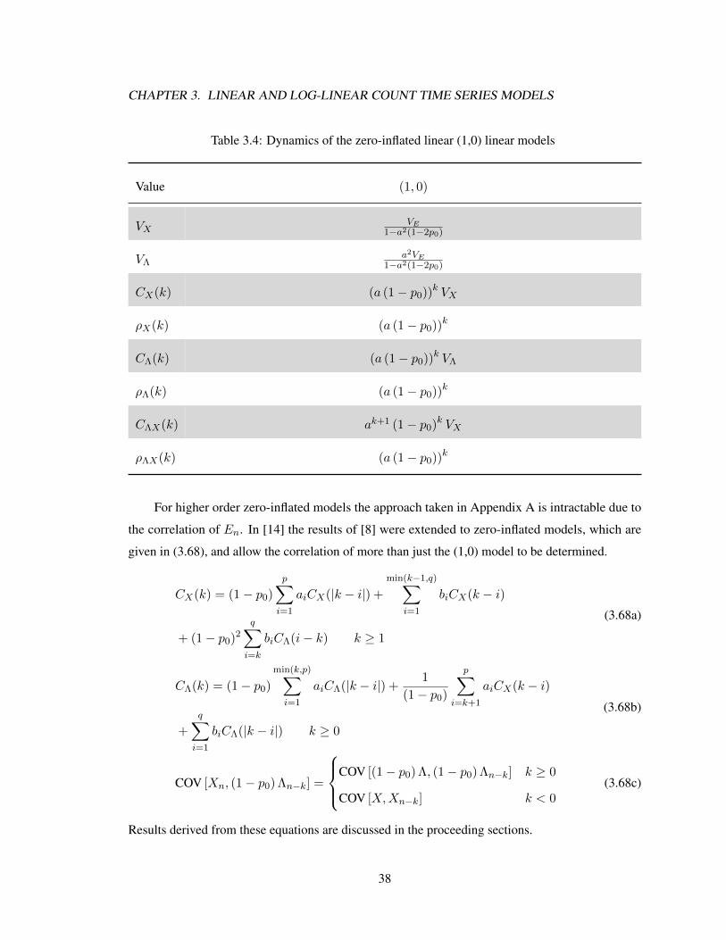
CHAPTER 3. LINEAR AND LOG-LINEAR COUNT TIME SERIES MODELS
Table 3.4: Dynamics of the zero-inflated linear (1,0) linear models
Value (1, 0)
VXVE
1−a2(1−2p0)
VΛa2VE
1−a2(1−2p0)
CX(k) (a (1− p0))k VX
ρX(k) (a (1− p0))k
CΛ(k) (a (1− p0))k VΛ
ρΛ(k) (a (1− p0))k
CΛX(k) ak+1 (1− p0)k VX
ρΛX(k) (a (1− p0))k
For higher order zero-inflated models the approach taken in Appendix A is intractable due to
the correlation of En. In [14] the results of [8] were extended to zero-inflated models, which are
given in (3.68), and allow the correlation of more than just the (1,0) model to be determined.
CX(k) = (1− p0)
p∑i=1
aiCX(|k − i|) +
min(k−1,q)∑i=1
biCX(k − i)
+ (1− p0)2q∑i=k
biCΛ(i− k) k ≥ 1
(3.68a)
CΛ(k) = (1− p0)
min(k,p)∑i=1
aiCΛ(|k − i|) +1
(1− p0)
p∑i=k+1
aiCX(k − i)
+
q∑i=1
biCΛ(|k − i|) k ≥ 0
(3.68b)
COV [Xn, (1− p0) Λn−k] =
COV [(1− p0) Λ, (1− p0) Λn−k] k ≥ 0
COV [X,Xn−k] k < 0(3.68c)
Results derived from these equations are discussed in the proceeding sections.
38

CHAPTER 3. LINEAR AND LOG-LINEAR COUNT TIME SERIES MODELS
3.6 The Linear ZIP INGARCH Model
To specialize the results of Table 3.4 to the ZIP model we require VE . Using the law of total
variance
VE = VAR [E [En|Z, In−1]] + E [VAR [En|Z, In−1]]
= p0 (−µΛ + p0µΛ)2 + (1− p0) (p0µΛ)2 + (1− p0) VAR [En|Zf ] + p0VΛ
= p0 (1− p0)µ2Λ + (1− p0) VAR [En|Zf ] + p0VΛ (3.69)
The form of (3.69) is convenient because it isolates the dependence of VE on the underlying
distribution. Substituting in for the Poisson distribution yields
VE = p0 (1− p0)µ2Λ + (1− p0)µΛ + p0VΛ
= µX (1 + p0µΛ) + p0VΛ (3.70)
Table 3.5 shows the results of applying (3.70) to Table 3.4. It also gives the results of Example
1 of [14], where the author examined the ZIP (1,1) model. One interesting consequence of zero-
inflation is that the region of stationarity is expanded. Table 3.5 shows that the (1,0) model is
stationary as long as
(1− p0) a < 1, a < 1 (3.71)
(1− p0) a2 < 1, a > 1 (3.72)
When a is less than one the region of stationarity is dictated by µΛ. Conversely, when a is greater
than one stationarity is restricted by VΛ. Solving for a in (3.72) and inserting into ρX(k) yields the
maximum possible value of ρX(1) for a given p0
max ρX(1) =√
(1− p0) (3.73)
Figure 3.11 shows the maximum allowable value of a for a given value of p0 as well as the maximum
achievable value of ρX(1). Similarly for the (1,1) model we find
(1− p0) a+ b < 1 (3.74)
(1− p0) a2 + 2 (1− p0) ab+ b2 < 1 (3.75)
must be true. Figure 3.12 shows the minimum value of p0 required to ensure stationarity of the (1,1)
model.
39

CHAPTER 3. LINEAR AND LOG-LINEAR COUNT TIME SERIES MODELS
Table 3.5: Dynamics of the ZIP (1,0) and (1,1) linear models
Value (1, 0) (1, 1)
VXµX(1+p0µΛ)1−(1−p0)a2
(µX+p0µXµΛ)(1−2(1−p0)ab−b2)1−(1−p0)a2−2(1−p0)ab−b2
VΛ a2 µX(1+p0µΛ)1−(1−p0)a2
a2(µX+p0µXµΛ)1−(1−p0)a2−2(1−p0)ab−b2
CX(k) (a (1− p0))k µX(1+p0µΛ)1−(1−p0)a2 ((1− p0) a+ b)k−1 (µX+p0µXµΛ)(1−p0)a(1−(1−p0)ab−b2)
1−(1−p0)a2−2(1−p0)ab−b2
ρX(k) (a (1− p0))k ((1− p0) a+ b)k−1 (1−p0)a(1−(1−p0)ab−b2)1−2(1−p0)ab−b2
CΛ(k) a2 (a (1− p0))k µX(1+p0µΛ)1−(1−p0)a2 ((1− p0) a+ b)k a2(µX+p0µXµΛ)
1−(1−p0)a2−2(1−p0)ab−b2
ρΛ(k) (a (1− p0))k ((1− p0) a+ b)k
Figure 3.13 shows several examples of the ZIP (1,0) model. Here d and a were held constant
while p0 was changed to explore the effects of p0. Figure 3.13a shows that even when p0 is small
the effect it has on the shape of the time series is considerable. Since feedback is only through xn
for the (1,0) model every instance of zero-inflation effectively resets the system. The result is that
the time series never appears to enter a steady state and is constantly in a state of growth towards
µΛ. Figure 3.13b and Figure 3.13c demonstrate how this effect becomes more pronounced as p0
increases. When p0 becomes large the shape of the time series becomes one of outliers amongst large
groups of zero values. The correlation of the time series is difficult to observe since it only occurs
when multiple non-zero values occur sequentially.
Figure 3.14 shows similar examples of the ZIP (1,1) model. Specifically when a feedback com-
ponent is included the effect of zero-inflation on the time series is drastically reduced. Figure 3.14a
and Figure 3.14b show that when b is large the effect of zero-inflation is reduced drastically on λn,
which is additionally reflected in xn where extraneous zeros only cause slight level shifts. When b is
decreased the effect of zero-inflation is more pronounced, as expected.
Finally, Figures 3.18a and 3.18b show examples of ZIP models with parameters outside the
region of stationarity for the Poisson model. Each shows exponential, non-stationary growth that
is reset by zero-inflation. Whether or not these models are of any practical use is unclear, but their
shape suggests they could model exponential growths periodically reset by some outside influence.
40

CHAPTER 3. LINEAR AND LOG-LINEAR COUNT TIME SERIES MODELS
0 0.2 0.4 0.6 0.8 1
p0
0
0.5
1
1.5
2
2.5
3
3.5
4
4.5
5
am
ax
0 0.1 0.2 0.3 0.4 0.5 0.6 0.7 0.8 0.9
p0
0.1
0.2
0.3
0.4
0.5
0.6
0.7
0.8
0.9
1
ma
x ρ
1Figure 3.11: The left plot shows the maximum allowable value of a as a function of p0 for the ZIP
(1,0) model. When values of a greater than 1 are used the resulting time series exhibits explosive
growth that is occasionally reset. The right plot shows the maximum possible value of ρX(1) as a
function of p0.
Figure 3.12: Minimum value of p0 to ensure stationarity for given a and b. Note that the region of
stationarity for b is not different from the Poisson model. When values outside the Poisson region of
stationarity are chosen the resulting time series exhibits exponential growth.
41

CHAPTER 3. LINEAR AND LOG-LINEAR COUNT TIME SERIES MODELS
(a) d = 5, a = 0.8, p0 = 0.1.
0 10 20 30 40 50 60 70 80 90 100
0
20
40
0 10 20 30 400
0.05
0.1
0.15
Marginal
0 5 10 15 20
k
0
0.5
1
ρX
X(k
)
Obs.Exp.
0 5 10 15 20
k
0
0.5
1
ρλλ(k
)
-10 -5 0 5 10
k
0
0.5
1
ρXλ(k
)
(b) d = 5, a = 0.8, p0 = 0.3.
0 10 20 30 40 50 60 70 80 90 100
0
10
20
30
0 10 20 30 400
0.2
0.4
Marginal
0 5 10 15 20
k
0
0.5
1
ρX
X(k
)
Obs.Exp.
0 5 10 15 20
k
0
0.5
1
ρλλ(k
)
-10 -5 0 5 10
k
0
0.5
1
ρXλ(k
)
(c) d = 5, a = 0.8, p0 = 0.5.
0 10 20 30 40 50 60 70 80 90 100
0
10
20
0 5 10 15 200
0.2
0.4
0.6
Marginal
0 5 10 15 20
k
0
0.5
1
ρX
X(k
)
Obs.Exp.
0 5 10 15 20
k
0
0.5
1
ρλλ(k
)
-10 -5 0 5 10
k
0
0.5
1
ρXλ(k
)
(d) d = 5, a = 0.8, p0 = 0.7.
0 10 20 30 40 50 60 70 80 90 100
0
5
10
15
0 5 10 15 200
0.5
1
Marginal
0 5 10 15 20
k
0
0.5
1
ρX
X(k
)
Obs.Exp.
0 5 10 15 20
k
0
0.5
1
ρλλ(k
)
-10 -5 0 5 10
k
0
0.5
1
ρXλ(k
)
Figure 3.13: Examples of the ZIP (1,0) model. Each plot shows from top right clockwise: xn in red
and λn in blue; The expected and observed ACF of Xn; The expected and observed cross-correlation
function of Xn and Λn; the expected and observed ACF of Λn; and the marginal distribution of a
time series of length 1 million
42

CHAPTER 3. LINEAR AND LOG-LINEAR COUNT TIME SERIES MODELS
(a) d = 5, a = 0.2, b = 0.7, p0 = 0.1.
0 10 20 30 40 50 60 70 80 90 100
0
20
40
60
20 30 40 50 60 700
0.05
0.1
0.15
Marginal
0 5 10 15 20
k
0
0.5
1
ρX
X(k
)
Obs.Exp.
0 5 10 15 20
k
0
0.5
1
ρλλ(k
)
-10 -5 0 5 10
k
0
0.5
1
ρXλ(k
)
(b) d = 5, a = 0.2, b = 0.7, p0 = 0.5.
0 10 20 30 40 50 60 70 80 90 100
0
20
40
10 15 20 25 30 35 400
0.2
0.4
0.6
Marginal
0 5 10 15 20
k
0
0.5
1
ρX
X(k
)
Obs.Exp.
0 5 10 15 20
k
0
0.5
1
ρλλ(k
)
-10 -5 0 5 10
k
0
0.5
1
ρXλ(k
)
(c) d = 5, a = 0.5, b = 0.4, p0 = 0.1.
0 10 20 30 40 50 60 70 80 90 100
0
20
40
60
10 20 30 40 50 600
0.05
0.1
Marginal
0 5 10 15 20
k
0
0.5
1
ρX
X(k
)
Obs.Exp.
0 5 10 15 20
k
0
0.5
1
ρλλ(k
)
-10 -5 0 5 10
k
0
0.5
1
ρXλ(k
)
(d) d = 5, a = 0.5, b = 0.4, p0 = 0.5.
0 10 20 30 40 50 60 70 80 90 100
0
10
20
10 15 20 25 300
0.2
0.4
0.6
Marginal
0 5 10 15 20
k
0
0.5
1
ρX
X(k
)
Obs.Exp.
0 5 10 15 20
k
0
0.5
1
ρλλ(k
)
-10 -5 0 5 10
k
0
0.5
1
ρXλ(k
)
Figure 3.14: Examples of the ZIP (1,1) model. Each plot shows from top right clockwise: xn in red
and λn in blue; The expected and observed ACF of Xn; The expected and observed cross-correlation
function of Xn and Λn; the expected and observed ACF of Λn; and the marginal distribution of a
time series of length 1 million
43

CHAPTER 3. LINEAR AND LOG-LINEAR COUNT TIME SERIES MODELS
3.7 The Linear ZINB2 Model
When data is zero-inflated and non-zero counts are over-dispersed compared to the ZIP linear
model, the ZINB2 linear model should be used. Substituting the variance of the NB2 distribution
into (3.69) yields
VE = p0 (1− p0)µ2Λ + (1− p0)
(µΛ +
VΛ + µ2Λ
ν
)+ p0VΛ
= µX
(1 + p0µΛ +
µΛ
ν
)+ VΛ
1 + p0ν
ν(3.76)
Inserting (3.76) into Table 3.4 produces the dynamics of the ZINB2 (1,0) model. Additionally, in [14]
the dynamics of the ZINB2 (1,1) model were found. These results are presented in Table 3.6. For the
ZINB2 (1,0) model to be second order stationary (3.77) must hold true.
(1− p0) a2 <ν
ν + 1(3.77)
Compared to (3.72) the parameter space is slightly more constrained. Figure 3.15 shows a contour
plot of the minimum value of ν needed to ensure stationarity as a function of a, and p0. Similarly for
the ZINB2 (1,1) model
1 + ν
ν(1− p0) a2 − 2 (1− p0) ab− b2 < 1 (3.78)
must hold true. The additional dispersion of the ZINB2 model does not change the theoretical ACF
compared to the ZIP model. In practice, however, the increased variability greatly increases the
required data length to ensure convergence of these values. This is exhibited in Figures 3.16 and 3.17
which show examples of ZINB2 (1,0) and (1,1) models. Figures 3.18c and 3.18d give examples of
the ZINB2 model with parameters outside the stationarity region of the NB2 model. The results are
similar to the ZIP model.
44

CHAPTER 3. LINEAR AND LOG-LINEAR COUNT TIME SERIES MODELS
Table 3.6: Dynamics of the ZINB2 (1,0) and (1,1) linear models
Value (1, 0) (1, 1)
VX ν(p0µXµΛ+µΛ+
µΛµXν )
1− (1+ν)ν
(1−p0)a2
(1−2(1−p0)ab−b2)(µX+
p0ν+1ν
µXµΛ
)1− 1+ν
ν(1−p0)a2−2(1−p0)ab−b2
VΛ a2ν(p0µXµΛ+µΛ+
µΛµXν )
1− (1+ν)ν
(1−p0)a2
a2(µX+p0µXµΛ+p0µXµΛ
ν )1− 1+ν
ν(1−p0)a2−2(1−p0)ab−b2
ρX(k) (a (1− p0))k ((1− p0) a+ b)k−1 (1−p0)a(1−(1−p0)ab−b2)1−2(1−p0)ab−b2
ρΛ(k) (a (1− p0))k ((1− p0) a+ b)k
Figure 3.15: Minimum allowable value of ν as a function of p0 and a for the ZINB2 (1,0) model.
45

CHAPTER 3. LINEAR AND LOG-LINEAR COUNT TIME SERIES MODELS
(a) d = 5, a = 0.8, ν = 2, p0 = 0.3.
0 10 20 30 40 50 60 70 80 90 100
0
20
40
60
0 5 10 15 200
0.2
0.4
Marginal
0 5 10 15 20
k
0
0.5
1
ρX
X(k
)
Obs.Exp.
0 5 10 15 20
k
0
0.5
1
ρλλ(k
)
-10 -5 0 5 10
k
0
0.5
1
ρXλ(k
)
(b) d = 5, a = 0.8, ν = 2, p0 = 0.3.
0 10 20 30 40 50 60 70 80 90 100
0
20
40
0 5 10 15 200
0.2
0.4
Marginal
0 5 10 15 20
k
0
0.5
1
ρX
X(k
)
Obs.Exp.
0 5 10 15 20
k
0
0.5
1
ρλλ(k
)
-10 -5 0 5 10
k
0
0.5
1
ρXλ(k
)
(c) d = 5, a = 0.8, ν = 2, p0 = 0.3.
0 10 20 30 40 50 60 70 80 90 100
0
10
20
0 5 10 15 200
0.2
0.4
Marginal
0 5 10 15 20
k
0
0.5
1
ρX
X(k
)
Obs.Exp.
0 5 10 15 20
k
0
0.5
1
ρλλ(k
)
-10 -5 0 5 10
k
0
0.5
1
ρXλ(k
)
(d) d = 5, a = 0.8, ν = 2, p0 = 0.3.
0 10 20 30 40 50 60 70 80 90 100
0
20
40
0 5 10 15 200
0.2
0.4
Marginal
0 5 10 15 20
k
0
0.5
1
ρX
X(k
)
Obs.Exp.
0 5 10 15 20
k
0
0.5
1
ρλλ(k
)
-10 -5 0 5 10
k
0
0.5
1
ρXλ(k
)
Figure 3.16: Examples of the ZINB2 (1,0) model. Each plot shows from top right clockwise:
xn in red and λn in blue; The expected and observed ACF of Xn; The expected and observed
cross-correlation function of Xn and Λn; the expected and observed ACF of Λn; and the marginal
distribution of a time series of length 1 million
46

CHAPTER 3. LINEAR AND LOG-LINEAR COUNT TIME SERIES MODELS
(a) d = 5, a = 0.2, b = 0.7, ν = 2, p0 = 0.2.
0 10 20 30 40 50 60 70 80 90 1000
50
100
0 10 20 30 40 500
0.1
0.2
0.3
Marginal
0 5 10 15 20
k
0
0.5
1
ρX
X(k
)
Obs.Exp.
0 5 10 15 20
k
0
0.5
1
ρλλ(k
)
-10 -5 0 5 10
k
0
0.5
1
ρXλ(k
)
(b) d = 5, a = 0.2, b = 0.7, ν = 10, p0 = 0.2.
0 10 20 30 40 50 60 70 80 90 100
0
20
40
60
0 10 20 30 40 500
0.1
0.2
Marginal
0 5 10 15 20
k
0
0.5
1
ρX
X(k
)
Obs.Exp.
0 5 10 15 20
k
0
0.5
1
ρλλ(k
)
-10 -5 0 5 10
k
0
0.5
1
ρXλ(k
)
(c) d = 5, a = 0.5, b = 0.4, ν = 2, p0 = 0.2.
0 10 20 30 40 50 60 70 80 90 100
0
20
40
60
80
0 10 20 30 40 500
0.1
0.2
0.3
Marginal
0 5 10 15 20
k
0
0.5
1
ρX
X(k
)
Obs.Exp.
0 5 10 15 20
k
0
0.5
1
ρλλ(k
)
-10 -5 0 5 10
k
0
0.5
1
ρXλ(k
)
(d) d = 5, a = 0.5, b = 0.4, ν = 10, p0 = 0.2.
0 10 20 30 40 50 60 70 80 90 100
0
20
40
0 10 20 30 40 500
0.1
0.2
0.3
Marginal
0 5 10 15 20
k
0
0.5
1
ρX
X(k
)
Obs.Exp.
0 5 10 15 20
k
0
0.5
1
ρλλ(k
)
-10 -5 0 5 10
k
0
0.5
1
ρXλ(k
)
Figure 3.17: Examples of the ZINB2 (1,1) model. Each plot shows from top right clockwise:
xn in red and λn in blue; The expected and observed ACF of Xn; The expected and observed
cross-correlation function of Xn and Λn; the expected and observed ACF of Λn; and the marginal
distribution of a time series of length 1 million
47

CHAPTER 3. LINEAR AND LOG-LINEAR COUNT TIME SERIES MODELS
(a) d = .5, a = 1.1, p0 = .25.
0 10 20 30 40 50 60 70 80 90 1000
50
100
0 10 20 30 400
0.2
0.4
0.6
Marginal
0 5 10 15 20
k
0
0.5
1
ρX
X(k
)
Obs.
Exp.
0 5 10 15 20
k
0
0.5
1
ρλλ(k
)
-10 -5 0 5 10
k
0
0.5
1
ρXλ(k
)
(b) d = .5, a = 0.8, b = .4, p0 = .4.
0 10 20 30 40 50 60 70 80 90 100
0
5
10
0 5 10 15 200
0.2
0.4
0.6
Marginal
0 5 10 15 20
k
0
0.5
1
ρX
X(k
)
Obs.
Exp.
0 5 10 15 20
k
0
0.5
1ρλλ(k
)
-10 -5 0 5 10
k
0
0.5
1
ρXλ(k
)
(c) d = .5, a = 1.1, ν = 6, p0 = .25.
0 10 20 30 40 50 60 70 80 90 100
0
10
20
30
0 5 10 15 200
0.2
0.4
0.6
Marginal
0 5 10 15 20
k
0
0.5
1
ρX
X(k
)
Obs.
Exp.
0 5 10 15 20
k
0
0.5
1
ρλλ(k
)
-10 -5 0 5 10
k
0
0.5
1
ρXλ(k
)
(d) d = .5, a = 0.7, b = .4, ν = 5p0 = .4.
0 10 20 30 40 50 60 70 80 90 100
0
10
20
30
0 5 10 15 200
0.2
0.4
0.6
Marginal
0 5 10 15 20
k
0
0.5
1
ρX
X(k
)
Obs.
Exp.
0 5 10 15 20
k
0
0.5
1
ρλλ(k
)
-10 -5 0 5 10
k
0
0.5
1
ρXλ(k
)
Figure 3.18: Examples of the ZIP and ZINB2 (1,0) and (1,1) model with regressive parameters
outside the stationarity space of the linear models. From top right clockwise the groups of plots
show: the ZIP (1,0) model; the ZIP (1,1) model; the ZINB2 (1,1) model; the ZINB2 (1,0) model.
48
CHAPTER 3. LINEAR AND LOG-LINEAR COUNT TIME SERIES MODELS
3.8 The Log-Linear Model
Although the linear model is well understood and analyzed, it is incapable of modeling negative
correlation. The so-called Poisson log-linear model has been studied in [2]. The log-linear model
takes advantage of the exponential function to allow the introduction of negative correlations. The
model is defined by a conditional Poisson distribution and the modified recursion given below
Xn ∼ Λ (λn = exp(νn),θ|In−1) (3.79)
νn = d+
p∑k=1
ak log(xn−k + 1) +
q∑k=1
bkνn−k (3.80)
0 ≤ |a|, |b| < 1 |a + b| < 1 (3.81)
Additionally, bounds on the model have been derived for the Poisson log-linear (1,1) model [15].
Attempts to generalize to higher order models is an area of current research. While the ability to
model negative correlations in count data is an exciting feature, its use in real world applications has
been limited as negatively correlated count data is not readily available [2].
For the Log-Linear Poisson model the authors of [2] have shown that
E [log(xn + 1)|νn = ν]− ν → 0 as ν →∞ (3.82)
Applying this to (3.80) assuming ν is reasonably large yields
ν =d
1−∑p
k=1 ak −∑q
k=1 bk(3.83)
µx = µλ = exp(ν) (3.84)
Theory and simulation show that a similar result cannot be found for the NB2, ZIP, and ZINB2
log-linear models. The effects of the model parameters on stationarity are unclear. While this topic is
discussed briefly in Section 4.7, this is an area of potential future work.
49

CHAPTER 3. LINEAR AND LOG-LINEAR COUNT TIME SERIES MODELS
3.9 Conclusion
This chapter demonstrated the capabilities of the linear and log-linear models in handling count
data. We focused predominately on linear models as their analysis is more tractable than log-linear
models. We showed that the marginal distribution of the Poisson model can be approximated by the
best fit NB2 distribution. This approximation is only valid for lengthy time series, however, and thus
is most useful as a heuristic tool to demonstrate the possible range of values the model can take. We
also demonstrated a simple method for ascertaining the bounds on the dispersion parameter for the
NB2 linear model. This technique relies on the well understood theory of ARMA models and should
be used to ensure stationarity of fitted NB2 models.
While the theoretical results for these models are interesting, ultimately the goal of time series
analysis is to use them to represent real world data. To do so requires knowledge of the model
parameters based on the data. In the next chapter we discuss methods for model parameter estimation
to bridge the gap between theory and application
50

CHAPTER 3. LINEAR AND LOG-LINEAR COUNT TIME SERIES MODELS
0 5 10 15 20 25 30 35 40 45 50
n
0
2
4
Co
un
t
0 2 4 6 8 10 12 14 16 18 20
k
-1
-0.5
0
0.5
1
ρX
X(k
)
0 5 10 15 20 25 30 35 40 45 50
n
0
2
4
6
Co
un
t
0 2 4 6 8 10 12 14 16 18 20
k
-1
-0.5
0
0.5
1
ρX
X(k
)
0 5 10 15 20 25 30 35 40 45 50
n
0
5
10
Co
un
t
0 2 4 6 8 10 12 14 16 18 20
k
-1
-0.5
0
0.5
1
ρX
X(k
)
0 5 10 15 20 25 30 35 40 45 50
n
10
20
30
Co
un
t
0 2 4 6 8 10 12 14 16 18 20
k
-1
-0.5
0
0.5
1
ρX
X(k
)
Figure 3.19: Examples of the log-linear Poisson (1,0) model. The left column shows and example
time series and its mean; the right column shows the corresponding ACF. From top to bottom
d = {0.5, 1.0, 2.5, 5.0} and in all instances a = −0.8. Observe that the ACF is no longer independent
of d.
51

CHAPTER 3. LINEAR AND LOG-LINEAR COUNT TIME SERIES MODELS
0 5 10 15 20 25 30 35 40 45 50
n
20
25
30
35
40
Co
un
t
0 2 4 6 8 10 12 14 16 18 20
k
-1
-0.5
0
0.5
1
ρX
X(k
)
0 5 10 15 20 25 30 35 40 45 50
n
0
5
10
15
Co
un
t
0 2 4 6 8 10 12 14 16 18 20
k
-1
-0.5
0
0.5
1
ρX
X(k
)
0 5 10 15 20 25 30 35 40 45 50
n
10
15
20
25
Co
un
t
0 2 4 6 8 10 12 14 16 18 20
k
-1
-0.5
0
0.5
1
ρX
X(k
)
0 5 10 15 20 25 30 35 40 45 50
n
0
5
10
15
Co
un
t
0 2 4 6 8 10 12 14 16 18 20
k
-1
-0.5
0
0.5
1
ρX
X(k
)
Figure 3.20: Examples of the log-linear Poisson (1,1) model. From top to bottom a =
{0.6,−0.5, 0.4,−0.8}, b = {−0.5,−0.3,−0.5, 0.4} and in all instances d = 3. Observe that
the value of a determines the shape of the ACF.
52
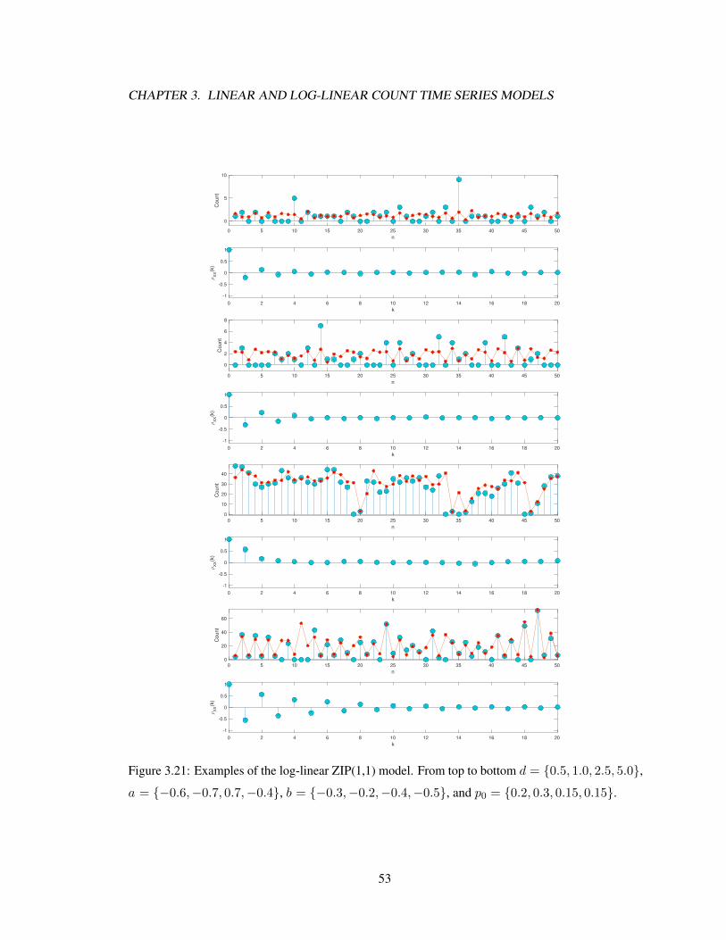
CHAPTER 3. LINEAR AND LOG-LINEAR COUNT TIME SERIES MODELS
0 5 10 15 20 25 30 35 40 45 50
n
0
5
10
Co
un
t
0 2 4 6 8 10 12 14 16 18 20
k
-1
-0.5
0
0.5
1
ρX
X(k
)
0 5 10 15 20 25 30 35 40 45 50
n
0
2
4
6
8
Co
un
t
0 2 4 6 8 10 12 14 16 18 20
k
-1
-0.5
0
0.5
1
ρX
X(k
)
0 5 10 15 20 25 30 35 40 45 50
n
0
10
20
30
40
Co
un
t
0 2 4 6 8 10 12 14 16 18 20
k
-1
-0.5
0
0.5
1
ρX
X(k
)
0 5 10 15 20 25 30 35 40 45 50
n
0
20
40
60
Co
un
t
0 2 4 6 8 10 12 14 16 18 20
k
-1
-0.5
0
0.5
1
ρX
X(k
)
Figure 3.21: Examples of the log-linear ZIP(1,1) model. From top to bottom d = {0.5, 1.0, 2.5, 5.0},a = {−0.6,−0.7, 0.7,−0.4}, b = {−0.3,−0.2,−0.4,−0.5}, and p0 = {0.2, 0.3, 0.15, 0.15}.
53

Chapter 4
Parameter Estimation in Count Time
Series Models
4.1 Introduction
Parameter estimation is an important topic in time series modeling as it bridges the gap between
theory and application. Estimation of linear and log-linear models has been studied by several
authors. The use of Conditional Maximum Likelihood Estimation for the Poisson linear model is
demonstrated in [1]. Similar results for the Poisson log-linear model are developed in [2]. The use
of Quasi Maximum Likelihood Estimation to estimate parameters of the NB2 linear model was
investigated in [3]. Last, the use of the expectation maximization algorithm to estimate parameters of
the ZIP and ZINB2 linear models was studied in [14].
This chapter focuses on the development and analysis of CMLE estimators for the NB2, ZIP,
and ZINB2 linear and log-linear models. The CMLE estimator for the Poisson linear model has
already been studied in [1]. The analysis is revisited here to serve as an example as well as to
provide symmetry. CMLE is an estimation technique that mirrors traditional Maximum Likelihood
Estimation (MLE) in that it relies on the likelihood function L (θ; x) where x = {xn, xn−1, . . . , x0}is a vector of observed counts. Typically the log-likelihood function L (θ; x) is used in place of
the likelihood function to simplify results since multiplication becomes addition. For CMLE the
Conditional Log-Likelihood (CLL) L (θ; x|In−1) is used in place of L (θ; x).
54

CHAPTER 4. PARAMETER ESTIMATION IN COUNT TIME SERIES MODELS
CMLE estimation relies on finding a solution to the equation Sn (θ) = 0 which, if it exists,
is denoted θ. The vector Sn (θ) is called the score vector and is defined as the gradient of the log-
likelihood function, given by (4.1). Also of importance are the observed information and cumulative
conditional information matrices, denoted by Hn (θ) and Gn (θ), respectively. The observed
information matrix is the Hessian of the log-likelihood, given by (4.2), whereas the cumulative
conditional matrix is the sum of conditional covariance matrices, given by (4.3). Under certain
regularity conditions −Hn (θ) equalsGn (θ) and both converge to the unconditional information
matrix G defined by (4.4) [16]. The matrix Hn (θ) also plays an important role in numerical
optimization algorithms that are used to solve nonlinear systems of equations, such as Sn (θ) = 0.
Sn (θ) =
N∑n=0
∂L (θ)
∂θ(4.1)
Hn (θ) =N∑n=0
∂2L (θ)
∂θ∂θT(4.2)
Gn (θ) =N∑n=0
VAR[∂L (θ)
∂θ
](4.3)
G = E [Gn (θ)] (4.4)
For notational simplicity, we use L (θ) in place of L (θ;xn|In−1) throughout the rest of the chapter.
The matrix G, although not explicitly calculable in many cases, is important because under the
assumptions of Section 1.4 of [16] it can be shown that√N(θ − θ
)p→ N (0,G(θ)−1) (4.5)
wherep→ denotes convergence in probability. Additionally, consistent estimators of G are given by
− 1NHn (θ) and 1
NGn (θ).
The rest of the chapter is broken into sections to develop and analyzeCMLE estimators for the
linear and log-linear models. Section 4.2 develops results needed for all linear models. Sections
4.3 through 4.6 derive the score and observed information matrices of the Poisson, NB2, ZIP, and
ZINB2 models, respectively. Each shows equivalence of the observed and conditional information.
Additionally, each section provides a simulation study to determine performance of the CMLE
estimators. Section 4.3 also develops approximations ofG for the (1,0) and (1,1) models. Section 4.4
compares results of the CMLE and Quasi Maximum Likelihood Estimation (QMLE) estimators.
Section 4.7 shows how the linear results can be easily adapted for log-linear models and provides the
results for each model.
55

CHAPTER 4. PARAMETER ESTIMATION IN COUNT TIME SERIES MODELS
4.2 Linear Count Time Series Model Estimation
Recall that the linear model is defined by (4.6)
λn = E [Xn|In−1] = d+
p∑k=1
akxn−k +
q∑k=1
bkλn−k (4.6)
Regardless of the underlying distribution, linear models are dependent on the model parameters
through the conditional mean. to apply CMLE therefore requires knowledge of the score of λn,
denoted by ∂λn∂θ , given in (4.7).
∂λn∂d
= 1 +
q∑k=1
bk∂λn−k∂d
(4.7a)
∂λn∂aj
= xn−j +
q∑k=1
bk∂λn−k∂aj
(4.7b)
∂λn∂bj
= λn−j +
q∑k=1
bk∂λn−k∂bj
(4.7c)
Knowledge of the Hessian of λn, denoted by ∂2λn∂θ∂θT , is required for numerical optimization as well
as approximation ofG and is given in (4.8).
∂2λn∂d2
=
q∑k=1
bk∂2λn∂d2
(4.8a)
∂2λn∂d∂aj
=
q∑k=1
bk∂2λn−k∂d∂aj
(4.8b)
∂2λn∂d∂bj
=∂λn−j∂d
+
q∑k=1
bk∂2λn−k∂d∂bj
(4.8c)
∂2λn∂aj∂ak
=
q∑k=1
bk∂2λn−k∂aj∂ak
(4.8d)
∂2λn∂bj∂bk
=∂λn−j∂bj
+∂λn−k∂bk
+
q∑k=1
bk∂2λn−k∂bj∂bk
(4.8e)
∂2λn∂aj∂bk
=∂λn−j∂aj
+
q∑k=1
bk∂2λn−k∂aj∂bk
(4.8f)
These equations form the backbone of CMLE for all linear models.
56

CHAPTER 4. PARAMETER ESTIMATION IN COUNT TIME SERIES MODELS
4.3 Poisson Linear Model Estimation
CMLE of the Poisson linear model has been studied extensively in [1], the main results of
which are re-derived for the purpose of exposition. Using the definition of the Poisson PMF (2.7) the
conditional likelihood and CLL are given by (4.9) and (4.10).
L (θ) =N∏n=0
exp(−λn)λxnnΓ(xn + 1)
(4.9)
L (θ) =N∑n=0
−λn + xn lnλn − ln Γ (xn + 1) (4.10)
Taking first and second derivatives of (4.10) with respect to θ and inserting the results into (4.1) and
(4.2) yields
Sn (θ) =N∑n=0
(xnλn− 1
)∂λn∂θ
(4.11)
Hn (θ) =N∑n=0
(xnλn− 1
)∂2λn∂θ∂θT
− xnλ2n
(∂λn∂θ
)(∂λn∂θ
)T
(4.12)
When xn is replaced by Xn and the expected value is taken (recalling the implicit assumption of the
expectation being conditioned on In−1) we find
E [Sn (θ)] = 0 (4.13)
E [Hn (θ)] =N∑n=0
− 1
λn
(∂λn∂θ
)(∂λn∂θ
)T
(4.14)
Since (B.3) equals zero (4.3) becomes
Gn (θ) =
N∑n=0
E
[(∂L (θ)
∂θ
)(∂L (θ)
∂θ
)T]
(4.15)
and simplifying
Gn (θ) =N∑n=0
E[(
Xn
λn− 1
)∂λn∂θ
(Xn
λn− 1
)∂λn∂θ
T]
=
N∑n=0
E
[(X2n
λ2n
− 2Xn
λn+ 1
)(∂λn∂θ
)(∂λn∂θ
)T]
57

CHAPTER 4. PARAMETER ESTIMATION IN COUNT TIME SERIES MODELS
Using the Poisson property of the conditional mean of Xn yields
Gn (θ) =N∑n=0
(λn + λ2
n
λ2n
− 2λnλn
+ 1
)(∂λn∂θ
)(∂λn∂θ
)T
=N∑n=0
1
λn
(∂λn∂θ
)(∂λn∂θ
)T
(4.16)
As expected −E [Hn (θ)] = Gn (θ) and thus
√N(θ − θ)
D−→ N(0,G−1) (4.17)
G = E[
1
λn
∂λn∂θ
∂λn∂θ
′](4.18)
A rigorous proof of this equality via the use of perturbed models is provided in [1].
As previously noted,G cannot always be found analytically; its value is of interest, however
because knowledge ofG provides important information about estimator convergence. We develop
and assess approximations ofG for the (1,0) and (1,1) models next. We use these approximations to
better understand convergence of CMLE for the (1,0) and (1,1) models.
To begin finding the approximation for the (1,0) model, denoted byG, we substitute(4.7a) and
(4.7b) into (4.18). Since there is no feedback of λn the information matrix G is only dependent on
the previous time-step
G = E
1λn
xn−1
λnxn−1
λn
x2n−1
λn
(4.19)
Next, we solve (4.6) for xn−1 and insert the result into (4.19) to obtain
G = E
1
λn
1− dλna
1− dλna
λn−2d+ d2
λna2
(4.20)
The quantity E[
1λn
]cannot be found analytically, therefore we use a second order Taylor Series
approximation about µΛ instead
Λ−1λ =
1
µΛ+VΛ
µ3Λ
(4.21)
Existence of this approximation is guaranteed since µΛ must be greater than zero. Using this
approximation in (4.20) yields
G =
Λ−1λ
1−dΛ−1λ
a1−dΛ−1
λa
µΛ−2d+d2Λ−1λ
a2
58

CHAPTER 4. PARAMETER ESTIMATION IN COUNT TIME SERIES MODELS
Expressing G in terms of the model parameters yields, upon simplification,
G =
(1−a)(a2+ad+d)d2(1+a)
a2−a+ad+dd+ad
a2−a+ad+dd+ad
1+a2+ad−2a+d1−a2
(4.22)
Inverting this matrix yields
G−1 =
d(1+a2+ad−2a+d)1−a a− d− ad− a2
a− d− ad− a2 (1−a)(a2+ad+d)d
(4.23)
We then use the derivatives of G−111 and G−1
22 with respect to d and a, where Xij represents the
value of row i, column j ofX , to determine how the values of d and a affect the bounds on θ.
∂G−11
∂d=
1 + a2 + 2ad− 2a+ 2d
1− a(4.24a)
∂G−11
∂a=d(−a2 + 2a+ 2d− 1
)(1− a)2 (4.24b)
∂G−14
∂d=−3a2 − 2ad+ 2a
d(4.24c)
∂G−14
∂a=
(a− 1) a2
d2(4.24d)
Several interesting observations can be made based on (4.24a) through (4.24d). First, (4.24a)
shows that as d increases the bound on d also increases. Next, (4.24b) demonstrates that as long
as d > .5a2 + a + .5 the confidence bound on d increases with respect to a. Continuing, based
on (4.24c) the bound on a decreases as d increases. Additionally as d increases indefinitely G−14
approaches (1− a)(a+ 1). This demonstrates that as long as d is large the bound on a is the same
regardless of the true value of d. Finally, (4.24d) shows that the bound on a is inversely proportional
to its value. Taken altogether these results are fascinating as they indicate that an increase in either
parameter values increases the bound on d and simultaneously decreases the bound on a.
We performed a simulation study to determine how well (4.22) and (4.23) approximate G
and G−1 across the parameter {a ∈ (0, 1)}×{d ∈ [.5, 100]}, where× represents the Cartesian
product. For each pair (d, a)G was estimated by averagingHn (θ) calculated at (d, a) across 1000
realizations ofX of length 1000. The result and its inverse were then compared to the estimates given
by (4.22) and (4.23). Contour plots of the normalized error of G and G−1 are given in Figure 4.1
and Figure 4.2. We observe that both G and G−1 show low error (±5%) except when d is small and
a is large. This can be attributed to Λ−1λ being a poor estimate for E
[1λn
]under these conditions.
59

CHAPTER 4. PARAMETER ESTIMATION IN COUNT TIME SERIES MODELS
Table 4.1: Standard errors of the approximate information matrix for the Poisson (1,0) Model vs.
observed standard errors. The first row (gray) for each combination shows the observed standard
errors from CMLE of 1000 series of length 1000. The second row shows the expected standard errors
found from G−1.
d a
0.1 0.2 0.3 0.4 0.5 0.6 0.7 0.8 0.9
0.5 (0.028, 0.034) (0.029, 0.035) (0.030, 0.035) (0.031, 0.034) (0.033, 0.033) (0.034, 0.030) (0.037, 0.027) (0.042, 0.023) (0.051, 0.016)
(0.027, 0.032) (0.028, 0.032) (0.029, 0.032) (0.030, 0.032) (0.032, 0.032) (0.035, 0.030) (0.040, 0.028) (0.048, 0.025) (0.069, 0.019)
2.0 (0.083, 0.032) (0.090, 0.032) (0.096, 0.031) (0.104, 0.030) (0.111, 0.028) (0.125, 0.026) (0.145, 0.023) (0.179, 0.020) (0.262, 0.014)
(0.082, 0.032) (0.087, 0.031) (0.094, 0.031) (0.103, 0.030) (0.114, 0.029) (0.130, 0.027) (0.153, 0.024) (0.191, 0.021) (0.276, 0.015)
5.0 (0.190, 0.032) (0.207, 0.032) (0.226, 0.031) (0.248, 0.029) (0.275, 0.027) (0.322, 0.026) (0.373, 0.023) (0.462, 0.019) (0.680, 0.014)
(0.187, 0.031) (0.204, 0.031) (0.223, 0.030) (0.248, 0.029) (0.278, 0.028) (0.319, 0.026) (0.378, 0.023) (0.475, 0.020) (0.690, 0.014)
10.0 (0.365, 0.032) (0.400, 0.031) (0.442, 0.030) (0.484, 0.029) (0.548, 0.027) (0.639, 0.026) (0.755, 0.023) (0.947, 0.019) (1.401, 0.014)
(0.362, 0.031) (0.397, 0.031) (0.439, 0.030) (0.489, 0.029) (0.552, 0.028) (0.636, 0.026) (0.755, 0.023) (0.950, 0.019) (1.379, 0.014)
20.0 (0.716, 0.032) (0.788, 0.031) (0.872, 0.030) (0.956, 0.029) (1.093, 0.027) (1.262, 0.025) (1.513, 0.023) (1.903, 0.019) (2.853, 0.014)
(0.712, 0.031) (0.785, 0.031) (0.870, 0.030) (0.972, 0.029) (1.100, 0.027) (1.268, 0.025) (1.508, 0.023) (1.898, 0.019) (2.757, 0.014)
Additionally, 1000 series of length 1000 were simulated at several pairs of (d, a). The standard
errors of these estimates was then compared to that expected byG. The results, shown in Table 4.1,
agree with the contour plots. They empirically show that increasing either parameter does in fact
increase the bound on d while simultaneously decreasing the bound on a. Additionally, as d increases
the standard error of a approaches (1−a)(a+1)N , as expected.
60

CHAPTER 4. PARAMETER ESTIMATION IN COUNT TIME SERIES MODELS
Figure 4.1: Contour plot of the normalized error of the 2x2 matrix estimate ofG. The x axis represents
a and the y axis represents d. G was estimated by averaging Gn (θ) over 1000 realizations of X
length 1000 at the true parameters
61

CHAPTER 4. PARAMETER ESTIMATION IN COUNT TIME SERIES MODELS
Figure 4.2: Contour plot of the normalized error of the 2x2 matrix estimate of G−1. The x axis
represents a and the y axis represents d. G was estimated by averagingGn (θ) over 1000 realizations
of X length 1000 at the true parameters
62
CHAPTER 4. PARAMETER ESTIMATION IN COUNT TIME SERIES MODELS
Next, we derive an approximation ofG for the (1,1) model. To begin we write each component
of ∂λn∂θ as an infinite sum
∂λn∂d
= 1 + b∂λn−1
∂d=
∞∑k=0
bk (4.25a)
∂λn∂a
= xn−1 + b∂λn−1
∂a=∞∑k=0
bkxn−k−1 (4.25b)
∂λn∂b
= λn−1 + b∂λn−1
∂b=∞∑k=0
bkλn−k−1 (4.25c)
Next, substituting Xn and Λn into (4.25b) and (4.25c) and taking expectation of each yields
E[∂λn∂d
]=
1
1− b(4.26a)
E[∂λn∂a
]=
µX1− b
(4.26b)
E[∂λn∂b
]=
µΛ
1− b(4.26c)
The second order Taylor series approximation ofG about µΛ is then
µzµ′z
µΛ+Hz − µzµ′z
µΛ+VΛ
µ3Λ
µzµ′z =
Hz
µΛ+VΛ
µ3Λ
µzµ′z (4.27)
where
µz = E[∂λn∂θ
]Hz = E
[∂λn∂θ
∂λn∂θ
′]We findHz by first multiplying (4.26a), (4.26b), and (4.26c) and taking expectations
E[∂λn∂d
∂λn∂d
]=
1
(1− b)2(4.28a)
E[∂λn∂d
∂λn∂a
]=
µX(1− b)2
(4.28b)
E[∂λn∂d
∂λn∂b
]=
µΛ
(1− b)2(4.28c)
Next, we find the cross terms between a and b. To begin observe that
E[∂λn∂a
∂λn∂a
]= E
[(xn−1 + b
∂λn−1
∂a
)2]
(4.29)
Expanding the inner term and simplifying yields
E[∂λn∂a
∂λn∂a
]= Rx(0) + b2E
[∂λn−1
∂a
∂λn−1
∂a
]+ 2bE
[Xn−1
∂λn−1
∂a
](4.30)
63

CHAPTER 4. PARAMETER ESTIMATION IN COUNT TIME SERIES MODELS
Using (4.25b) the third term becomes
E[Xn−1
∂λn−1
∂a
]= E
[Xn−1
∞∑i=0
biXn−1−i
]
=
∞∑i=0
biRx(i+ 1)
=∞∑i=0
bi
(µ2X + µX
a (1− b (a+ b)) (a+ b)i
1− (a+ b)2
)
=µ2X
1− b+
aµX
1− (a+ b)2 (4.31)
Plugging (4.31) back into (4.30) and solving yields
E[∂λn∂a
∂λn∂a
]=
µ2X
(1− b)2 +µX
1− (a+ b)2 (4.32)
Following a similar procedure yields
E[∂λn∂a
∂λn∂b
]=
µ2X
(1− b)2 +a (a+ b) µX(
1− (a+ b)2)
(1− b (a+ b))(4.33)
E[∂λn∂b
∂λn∂b
]=
µ2X
(1− b)2 +a2µX (1 + b (a+ b))
(1− b (a+ b)) (1− b)2 (4.34)
Figure 4.3 shows the normalized error of G for the (1,1) model for d = {.5, 5.10}. We observe
that there is a large error when d is small. This error decreases however, as d increases. Tables
4.2, 4.3, and 4.4 show how well the approximation performs, comparing the expected and observed
standard errors using a similar simulation to that for the (1,0) model. We observe that, interestingly,
the bounds on a and b appear to be unaffected by the value of d. Additionally, we observe that the
bounds on a and b both decrease as either parameter increases.
64

CHAPTER 4. PARAMETER ESTIMATION IN COUNT TIME SERIES MODELS
Table 4.2: Standard errors of the approximate information matrix for the Poisson(1,1) model vs.
observed standard errors for d = .5. The first row (gray) for each combination shows the observed
standard error from CMLE of 1000 series of length 1000. The second row shows the expected
standard errors found from G−1.
b a
0.1 0.2 0.3 0.4 0.5 0.6 0.7 0.8
0.1 (0.111, 0.031, 0.179) (0.083, 0.033, 0.115) (0.070, 0.035, 0.087) (0.061, 0.034, 0.066) (0.062, 0.035, 0.057) (0.060, 0.034, 0.047) (0.058, 0.033, 0.041) (0.067, 0.035, 0.037)
(0.191, 0.032, 0.308) (0.107, 0.032, 0.153) (0.081, 0.032, 0.101) (0.070, 0.032, 0.075) (0.066, 0.032, 0.059) (0.066, 0.032, 0.049) (0.072, 0.032, 0.041) (0.093, 0.031, 0.036)
0.2 (0.138, 0.033, 0.197) (0.107, 0.034, 0.133) (0.083, 0.034, 0.093) (0.072, 0.034, 0.070) (0.063, 0.034, 0.053) (0.068, 0.033, 0.044) (0.074, 0.033, 0.039) —
(0.204, 0.032, 0.291) (0.113, 0.032, 0.143) (0.086, 0.031, 0.093) (0.074, 0.031, 0.068) (0.071, 0.031, 0.053) (0.075, 0.031, 0.043) (0.093, 0.031, 0.036) —
0.3 (0.171, 0.031, 0.210) (0.122, 0.033, 0.132) (0.095, 0.035, 0.090) (0.081, 0.032, 0.063) (0.073, 0.032, 0.048) (0.082, 0.032, 0.038) — —
(0.213, 0.031, 0.265) (0.118, 0.031, 0.128) (0.090, 0.031, 0.082) (0.079, 0.031, 0.060) (0.078, 0.031, 0.046) (0.094, 0.030, 0.037) — —
0.4 (0.204, 0.031, 0.210) (0.132, 0.032, 0.119) (0.096, 0.032, 0.074) (0.081, 0.033, 0.051) (0.091, 0.032, 0.041) — — —
(0.220, 0.031, 0.232) (0.122, 0.031, 0.110) (0.093, 0.030, 0.070) (0.085, 0.030, 0.049) (0.096, 0.030, 0.037) — — —
0.5 (0.242, 0.029, 0.203) (0.135, 0.031, 0.096) (0.098, 0.031, 0.058) (0.101, 0.030, 0.041) — — — —
(0.222, 0.030, 0.192) (0.124, 0.030, 0.089) (0.098, 0.029, 0.055) (0.100, 0.028, 0.038) — — — —
0.6 (0.280, 0.029, 0.180) (0.141, 0.029, 0.073) (0.114, 0.028, 0.042) — — — — —
(0.219, 0.029, 0.147) (0.125, 0.028, 0.066) (0.109, 0.027, 0.039) — — — — —
0.7 (0.288, 0.028, 0.130) (0.150, 0.025, 0.046) — — — — — —
(0.209, 0.026, 0.099) (0.129, 0.025, 0.042) — — — — — —
0.8 (0.305, 0.022, 0.072) — — — — — — —
(0.193, 0.022, 0.053) — — — — — — —
Table 4.3: Standard errors of the approximate information matrix for the Poisson(1,1) model vs.
observed standard errors for d = 5. The first row (gray) for each combination shows the observed
standard error from CMLE of 1000 series of length 1000. The second row shows the expected
standard errors found from G−1.
b a
0.1 0.2 0.3 0.4 0.5 0.6 0.7 0.8
0.1 (1.148, 0.032, 0.190) (0.786, 0.031, 0.116) (0.646, 0.032, 0.083) (0.596, 0.033, 0.069) (0.602, 0.032, 0.055) (0.574, 0.031, 0.045) (0.647, 0.033, 0.043) (0.835, 0.032, 0.036)
(1.899, 0.032, 0.308) (1.048, 0.032, 0.153) (0.777, 0.032, 0.101) (0.656, 0.032, 0.075) (0.603, 0.032, 0.059) (0.594, 0.032, 0.049) (0.639, 0.032, 0.041) (0.808, 0.031, 0.036)
0.2 (1.440, 0.032, 0.213) (1.021, 0.030, 0.130) (0.815, 0.033, 0.093) (0.721, 0.031, 0.071) (0.658, 0.031, 0.053) (0.706, 0.032, 0.044) (0.825, 0.032, 0.039) —
(2.027, 0.032, 0.291) (1.113, 0.032, 0.143) (0.825, 0.031, 0.093) (0.701, 0.031, 0.068) (0.655, 0.031, 0.053) (0.676, 0.031, 0.043) (0.826, 0.031, 0.036) —
0.3 (1.694, 0.031, 0.212) (1.157, 0.031, 0.127) (0.900, 0.031, 0.085) (0.759, 0.031, 0.060) (0.730, 0.031, 0.047) (0.893, 0.031, 0.037) — —
(2.126, 0.031, 0.265) (1.166, 0.031, 0.128) (0.868, 0.031, 0.082) (0.749, 0.031, 0.060) (0.729, 0.031, 0.046) (0.852, 0.030, 0.037) — —
0.4 (2.030, 0.030, 0.214) (1.306, 0.032, 0.119) (0.967, 0.029, 0.071) (0.869, 0.031, 0.051) (0.919, 0.030, 0.038) — — —
(2.192, 0.031, 0.232) (1.204, 0.031, 0.110) (0.907, 0.030, 0.070) (0.812, 0.030, 0.049) (0.892, 0.030, 0.037) — — —
0.5 (2.318, 0.031, 0.195) (1.309, 0.030, 0.093) (0.999, 0.029, 0.057) (0.981, 0.029, 0.038) — — — —
(2.214, 0.030, 0.192) (1.225, 0.030, 0.089) (0.952, 0.029, 0.055) (0.954, 0.028, 0.038) — — — —
0.6 (2.644, 0.028, 0.171) (1.263, 0.028, 0.067) (1.130, 0.028, 0.039) — — — — —
(2.184, 0.029, 0.147) (1.235, 0.028, 0.066) (1.061, 0.027, 0.039) — — — — —
0.7 (2.696, 0.025, 0.120) (1.381, 0.026, 0.045) — — — — — —
(2.088, 0.026, 0.099) (1.277, 0.025, 0.042) — — — — — —
0.8 (2.597, 0.021, 0.064) — — — — — — —
(1.930, 0.022, 0.053) — — — — — — —
65

CHAPTER 4. PARAMETER ESTIMATION IN COUNT TIME SERIES MODELS
Table 4.4: Standard errors of the approximate information matrix for the Poisson(1,1) model vs.
observed standard errors for d = 10. The first row (gray) for each combination shows the observed
standard error from CMLE of 1000 series of length 1000. The second row shows the expected
standard errors found from G−1.
b a
0.1 0.2 0.3 0.4 0.5 0.6 0.7 0.8
0.1 (2.305, 0.030, 0.191) (1.618, 0.033, 0.121) (1.376, 0.032, 0.091) (1.235, 0.033, 0.068) (1.152, 0.032, 0.056) (1.157, 0.031, 0.046) (1.290, 0.032, 0.041) (1.607, 0.032, 0.037)
(3.797, 0.032, 0.308) (2.093, 0.032, 0.153) (1.550, 0.032, 0.101) (1.307, 0.032, 0.075) (1.197, 0.032, 0.059) (1.178, 0.032, 0.049) (1.263, 0.032, 0.041) (1.593, 0.031, 0.036)
0.2 (2.827, 0.033, 0.208) (2.018, 0.033, 0.130) (1.665, 0.031, 0.094) (1.432, 0.032, 0.070) (1.381, 0.031, 0.055) (1.431, 0.029, 0.044) (1.660, 0.032, 0.036) —
(4.052, 0.032, 0.291) (2.224, 0.032, 0.143) (1.647, 0.031, 0.093) (1.397, 0.031, 0.068) (1.303, 0.031, 0.053) (1.340, 0.031, 0.043) (1.634, 0.031, 0.036) —
0.3 (3.466, 0.032, 0.219) (2.369, 0.031, 0.129) (1.633, 0.031, 0.079) (1.539, 0.032, 0.062) (1.405, 0.031, 0.045) (1.875, 0.030, 0.037) — —
(4.252, 0.031, 0.265) (2.330, 0.031, 0.128) (1.732, 0.031, 0.082) (1.492, 0.031, 0.060) (1.450, 0.031, 0.046) (1.691, 0.030, 0.037) — —
0.4 (3.908, 0.029, 0.204) (2.648, 0.031, 0.119) (1.968, 0.032, 0.074) (1.600, 0.029, 0.047) (1.823, 0.029, 0.036) — — —
(4.383, 0.031, 0.232) (2.405, 0.031, 0.110) (1.810, 0.030, 0.070) (1.618, 0.030, 0.049) (1.774, 0.030, 0.037) — — —
0.5 (4.419, 0.027, 0.187) (2.714, 0.030, 0.095) (1.907, 0.028, 0.053) (2.068, 0.028, 0.039) — — — —
(4.428, 0.030, 0.192) (2.448, 0.030, 0.089) (1.901, 0.029, 0.055) (1.902, 0.028, 0.038) — — — —
0.6 (5.140, 0.029, 0.168) (2.788, 0.028, 0.071) (2.322, 0.026, 0.039) — — — — —
(4.367, 0.029, 0.147) (2.468, 0.028, 0.066) (2.117, 0.027, 0.039) — — — — —
0.7 (5.485, 0.027, 0.122) (2.905, 0.026, 0.045) — — — — — —
(4.175, 0.026, 0.099) (2.552, 0.025, 0.042) — — — — — —
0.8 (5.128, 0.022, 0.064) — — — — — — —
(3.860, 0.022, 0.053) — — — — — — —
To assess the CMLE estimator for the Poisson model we performed a Monte Carlo simulation
generating 1000 series of length 200 and 1000 for each of the models below. The series were then fit
with the appropriate model.
• A1: (d, a1) = (0.5, 0.4)
• A2: (d, a1) = (0.5, 0.8)
• A3: (d, a1) = (1.0, 0.4)
• A4: (d, a1) = (1.0, 0.8)
• A5: (d, a1) = (4.0, 0.5)
• B1: (d, a1, a2) = (0.5, 0.4, 0.4)
• B2: (d, a1, a2) = (0.5, 0.7, 0.2)
• B3: (d, a1, a2) = (1.0, 0.4, 0.4)
• B4: (d, a1, a2) = (1.0, 0.7, 0.2)
• B5: (d, a1, a2) = (4.0, 0.2, 0.2)
• C1: (d, a1, b1) = (0.5, 0.3, 0.6)
• C2: (d, a1, b1) = (0.5, 0.7, 0.2)
• C3: (d, a1, b1) = (1.0, 0.3, 0.6)
• C4: (d, a1, b1) = (1.0, 0.7, 0.2)
• C5: (d, a1, b1) = (4.0, 0.4, 0.4)
Results of the aggregate set of estimators for each model are given in Tables 4.5, 4.6, and 4.7.
Each table shows the model, the length of the series, and the estimators. For each estimator the
mean of the aggregate set is shown. In parenthesis the observed standard error is reported next to
the expected standard error. The expected standard error was found be calculating the observed
66

CHAPTER 4. PARAMETER ESTIMATION IN COUNT TIME SERIES MODELS
Table 4.5: CMLE results for the Poisson linear (1,0) model. For each model 1000 series of length N
were simulated. The first number in each column shows the mean of the estimator. In parenthesis are
the observed and expected standard errors.
Model N d a1
A1 200 0.5069(0.0725,0.0698) 0.3904(0.0735,0.0760)
1000 0.5024(0.0311,0.0311) 0.3972(0.0335,0.0340)
A2 200 0.5259(0.0991,0.0916) 0.7831(0.0517,0.0502)
1000 0.5035(0.0419,0.0409) 0.7978(0.0228,0.0224)
A3 200 1.0152(0.1198,0.1230) 0.3887(0.0699,0.0696)
1000 1.0004(0.0550,0.0552) 0.3985(0.0314,0.0312)
A4 200 1.0696(0.2212,0.1882) 0.7816(0.0493,0.0451)
1000 1.0142(0.0861,0.0837) 0.7963(0.0199,0.0200)
A5 200 4.1091(0.5060,0.4994) 0.4852(0.0638,0.0625)
1000 4.0176(0.2246,0.2218) 0.4975(0.0278,0.0277)
information and conditional information matrices at the true parameters θ for each series and taking
the average of each. The sandwich estimatorHn (θ)Gn (θ)−1Hn (θ) was then used to determine
the expected standard errors.
The results in Table 4.7 are similar to those of [1]. There is a slight bias observed in d for all
models however. Table 4.5 shows that increasing a1 increases this bias. Table 4.6 shows similar
results for the (2,0) model that suggest this bias is due to correlation in the data. The bias is worst for
the (1,1) model (Table 4.7), where it appears that increasing b1 actually has a more drastic effect on
this bias than increasing a1.
67

CHAPTER 4. PARAMETER ESTIMATION IN COUNT TIME SERIES MODELS
Table 4.6: CMLE results for the Poisson linear (1,0) model. For each model 1000 series of length N
were simulated. The first number in each column shows the mean of the estimator. In parenthesis are
the observed and expected standard errors.
Model N d a1 a2
B1 200 0.5484(0.1337,0.1181) 0.3914(0.0730,0.0692) 0.3809(0.0701,0.0691)
1000 0.5097(0.0534,0.0521) 0.3980(0.0315,0.0310) 0.3956(0.0305,0.0309)
B2 200 0.5698(0.1608,0.1333) 0.6951(0.0777,0.0711) 0.1828(0.0744,0.0698)
1000 0.5131(0.0621,0.0592) 0.7008(0.0323,0.0318) 0.1946(0.0320,0.0312)
B3 200 1.1114(0.2860,0.2444) 0.3942(0.0719,0.0666) 0.3795(0.0698,0.0666)
1000 1.0235(0.1158,0.1095) 0.3993(0.0301,0.0297) 0.3956(0.0281,0.0296)
B4 200 1.1944(0.3856,0.2980) 0.6973(0.0728,0.0695) 0.1797(0.0718,0.0692)
1000 1.0443(0.1362,0.1327) 0.7004(0.0309,0.0310) 0.1947(0.0303,0.0308)
B5 200 4.1633(0.6104,0.5809) 0.1918(0.0737,0.0703) 0.1830(0.0702,0.0703)
1000 4.0339(0.2558,0.2589) 0.1990(0.0303,0.0314) 0.1956(0.0309,0.0314)
Table 4.7: CMLE results for the Poisson linear (1,0) model. For each model 1000 series of length N
were simulated. The first number in each column shows the mean of the estimator. In parenthesis are
the observed and expected standard errors.
Model N d a1 b1
C1 200 0.6864(0.3547,0.2383) 0.2950(0.0625,0.0608) 0.5662(0.1056,0.0886)
1000 0.5326(0.1169,0.1053) 0.2975(0.0282,0.0271) 0.5962(0.0414,0.0394)
C2 200 0.6026(0.2059,0.1582) 0.6987(0.0769,0.0710) 0.1754(0.0884,0.0815)
1000 0.5234(0.0759,0.0701) 0.7029(0.0325,0.0315) 0.1916(0.0380,0.0360)
C3 200 1.3522(0.6891,0.4740) 0.2944(0.0630,0.0592) 0.5699(0.1009,0.0867)
1000 1.0658(0.2270,0.2115) 0.2974(0.0262,0.0270) 0.5959(0.0392,0.0392)
C4 200 1.2310(0.4173,0.3336) 0.6939(0.0746,0.0689) 0.1809(0.0858,0.0801)
1000 1.0446(0.1597,0.1489) 0.7004(0.0308,0.0310) 0.1949(0.0354,0.0360)
C5 200 4.7148(1.7447,1.4705) 0.3893(0.0714,0.0683) 0.3745(0.1208,0.1129)
1000 4.1399(0.6663,0.6433) 0.4005(0.0313,0.0300) 0.3924(0.0510,0.0492)
68

CHAPTER 4. PARAMETER ESTIMATION IN COUNT TIME SERIES MODELS
Figure 4.3: Contour plot of the error of the approximate information matrix for the Poisson (1,1)
model. The x axis is the value of a and the y axis is the value of b, hence the upper half of each plot
is an undefined region in blue. The columns, from left to right, represent the normalized error of the
information for d, a, and b.
69

CHAPTER 4. PARAMETER ESTIMATION IN COUNT TIME SERIES MODELS
4.4 Negative Binomial Linear Model Estimation
Estimation of the NB2 model can be performed in several different manners. One approach is to
use the QMLE estimator proposed by [3]. Alternatively, CMLE can be performed via maximization
of the CLL. This section provides a brief overview of the QMLE as well as an alternative CMLE
estimator. The simulation study in this section uses both the QMLE and the CMLE to compare the
two.
In [3] estimation of the NB2 model via QMLE was explored. One of the benefits of QMLE is
that it is adaptable to many different distributions. This comes at the expense of having to correct the
observed information matrix to find bounds on θ. Additionally any distributional parameters must be
estimated via alternative methods. Depending on the method bounds on these parameters may need
to be found via bootstrapping. In [3] conditional Poisson distribution was assumed and it was found
that under this assumption the cumulative conditional information matrix is
Gn (θ) =∞∑n=1
(1
λn+
1
ν
)(∂λn∂θ
)(∂λn∂θ
)T
They also showed that asymptotically the QMLE estimate converges as
√N(θ − θ
)D−→ N
(0, G−1 (θ)G1 (θ)G−1 (θ)
)G (θ) = E
[1
λn
(∂λn∂θ
)(∂λn∂θ
)T]
G1 (θ) = E
[(1
λn+
1
ν
)(∂λn∂θ
)(∂λn∂θ
)T]
Additionally, they suggested using one of the either (4.35) or (4.36), due to Gourieroux and Breslow
in [3], respectively, to estimate ν. In (4.36) M represents the number of model parameters that were
estimated.
ν =
1
N
N∑n=1
(xn − λn
)2− λn
λ2n
−1
(4.35)
N −M =N∑n=1
(xn − λn
)2
λn
(1 + λn
ν
) (4.36)
Equation (4.36) must be solved for ν using an additional maximization scheme.
70

CHAPTER 4. PARAMETER ESTIMATION IN COUNT TIME SERIES MODELS
To derive CMLE for the NB2 model we need the conditional likelihood and CLL, given in
(4.37) and (4.38).
L (θ, ν) =N∏n=0
Γ (xn + ν)
Γ (ν) Γ (xn + 1)
(ν
λn + ν
)ν ( λnλn + ν
)xn(4.37)
L (θ, ν) =N∑n=0
ln Γ (xn + ν)− ln Γ (xn + 1)− ln Γ (ν)
+ ν [ln ν − ln (λn + ν)] + xn [lnλn − ln (λn + ν)]
(4.38)
Taking derivatives of (4.38) with respect to θ and ν yields (4.39a) and (4.39b) where Ψ (x) is the
digamma function defined as the first derivative of ln Γ (x). The quantity Sn (θ) is then given by
(4.39c).
∂L (θ, ν)
∂θ=ν(xn − λn)
λn(λn + ν)
∂λn∂θ
(4.39a)
∂L (θ, ν)
∂ν= Ψ (xn + ν)−Ψ (ν) + ln(ν)− ln(λn + ν) + 1− (ν + xn)
λn + ν(4.39b)
Sn (θ) =N∑n=0
(∂L(θ,ν)∂θ
∂L(θ,ν)∂ν
)T(4.39c)
While the expected value of (4.39a) is 0, it is not apparent whether this is true for (4.39b). In practice,
it appears safe to assume the expected value of (4.39b) is 0. Further differentiation of (4.39a) and
(4.39b) yieldsHn (θ), where ψ′(x) is the second derivative of ln Γ (x).
∂2L (θ, ν)
∂ν2= Ψ′ (xn + ν)−Ψ′ (ν) +
xnν + λ2n
ν (λn + ν)2 (4.40a)
∂2L (θ, ν)
∂θ∂θT=ν(xn − λn)
λn(λn + ν)
∂2λn∂θ∂θT
− ν(−λ2n + νxn + 2xnλn)
λ2n(λn + ν)2
(∂λn∂θ
)(∂λn∂θ
)T
(4.40b)
∂2L (θ, ν)
∂ν∂θ=
xn − λn(λn + ν)2
∂λn∂θ
(4.40c)
Hn (θ) =
N∑n=0
∂2L(θ,ν)∂θ∂θT
∂2L(θ,ν)∂ν∂θ
T
∂2L(θ,ν)∂ν∂θ
∂2L(θ,ν)∂ν2
(4.40d)
71

CHAPTER 4. PARAMETER ESTIMATION IN COUNT TIME SERIES MODELS
Replacing xn with Xn and finding the expectation ofHn (θ) (conditioned on In−1) produces
E[∂2L (θ, ν)
∂ν2
]=
N∑n=0
E[Ψ′ (xn + ν)
]−Ψ′ (ν) +
λnν(λn + ν)
(4.41a)
E[∂2L (θ, ν)
∂θ∂θT
]= −
N∑n=0
ν
λn(λn + ν)
(∂λn∂θ
)(∂λn∂θ
)T
(4.41b)
E[∂2L (θ, ν)
∂ν∂θ
]= 0 (4.41c)
Additionally,Gn (θ) is given by
Gn (θ) =N∑n=0
VAR[∂L(θ,ν)∂θ
]COV
[∂L(θ,ν)∂θ , ∂L(θ,ν)
∂ν
]T
COV[∂L(θ,ν)∂θ , ∂L(θ,ν)
∂ν
]VAR
[∂L(θ,ν)∂ν
] (4.42)
Expanding the first term yields
VAR[∂L (θ)
∂θ
]= E
[(ν(Xn − λn)
λn(λn + ν)
)∂λn∂θ
(ν(Xn − λn)
λn(λn + ν)
)∂λn∂θ
T]which follows since the expected value of (4.39a) is 0. Simplifying,
VAR[∂L (θ)
∂θ
]= E
[(ν2(X2n − 2Xnλn + λ2
n
)λ2n(λn + ν)2
)(∂λn∂θ
)(∂λn∂θ
)T]
Since Xn|In−1 is an NB2 random variable E[X2n
]= λn + λ2
nν + λ2
n and
VAR[∂L (θ)
∂θ
]=
ν2(λn + λ2
nν + λ2
n − λ2n
)λ2n(λn + ν)2
(∂λn∂θ
)(∂λn∂θ
)T
=ν
λn(λn + ν)
(∂λn∂θ
)(∂λn∂θ
)T
(4.43)
If
VAR[∂L (θ)
∂ν
]=
N∑n=0
−E[Ψ′ (xn + ν)
]+ Ψ′ (ν)− λn
ν(λn + ν)(4.44)
E[∂L (θ)
∂ν
∂L (θ)
∂θ
]= 0 (4.45)
are both satisfied then Hn (θ) and Gn (θ) are consistent with one another and each can be used to
approximateG and
G = E
[ν
λn(λn + ν)
(∂λn∂θ
)(∂λn∂θ
)T]
(4.46)
72

CHAPTER 4. PARAMETER ESTIMATION IN COUNT TIME SERIES MODELS
It is interesting to note that the (4.41c) equals 0. This helps justify the use of a technique such as
QMLE since in CMLE estimation of ν is still effectively decoupled from estimation of the model
parameters.
We performed a simulation study similar to that for the Poisson model. An identical methodology
was used to assess performance of CMLE on the models given below. In addition QMLE was
evaluated for each model; only the results of ν2 are reported since [3] found this estimator to perform
better than ν1 in all cases.
• A1: (d, a1, ν) = (0.5, 0.4, 2.0)
• A2: (d, a1, ν) = (0.5, 0.4, 3.0)
• A3: (d, a1, ν) = (0.5, 0.8, 5.0)
• A4: (d, a1, ν) = (5.0, 0.5, 2.0)
• A5: (d, a1, ν) = (5.0, 0.5, 5.0)
• B1: (d, a1, a2, ν) = (0.5, 0.4, 0.4, 2.0)
• B2: (d, a1, a2, ν) = (0.5, 0.4, 0.4, 5.0)
• B3: (d, a1, a2, ν) = (0.5, 0.2, 0.6, 2.0)
• B4: (d, a1, a2, ν) = (0.5, 0.6, 0.2, 5.0)
• B5: (d, a1, a2, ν) = (5.0, 0.4, 0.4, 5.0)
• C1: (d, a1, b1, ν) = (0.5, 0.5, 0.3, 2.0)
• C2: (d, a1, b1, ν) = (0.5, 0.5, 0.3, 5.0)
• C3: (d, a1, b1, ν) = (0.5, 0.5, 0.4, 2.0)
• C4: (d, a1, b1, ν) = (0.5, 0.4, 0.4, 5.0)
• C5: (d, a1, b1, ν) = (4.0, 0.4, 0.4, 5.0)
The results for the CMLE estimator are given in Tables 4.8, through 4.10. The results for the
QMLE estimator are given in Tables 4.8 through 4.10. Comparing the two estimators shows that they
give comparable results. One observation of note is that for both estimation techniques models with
larger valued dispersion parameters can have biased estimators for short time series. This occurs
when the underlying data is well modeled by the Poisson model and ν becomes large. This effect
diminishes as the length of the time series increases.
Table 4.14 compares the observed and conditional information matrices of several models. For
each model Hn (θ) and Gn (θ) were evaluated at the true parameters θ for 1000 simulated time
series of length 1000. These values were then averaged and standardized to produce estimates ofG.
The first row for each N shows G based on the observed information and the second row shows G
based on the conditional information. In all cases the Matrices show conversion to one another.
73

CHAPTER 4. PARAMETER ESTIMATION IN COUNT TIME SERIES MODELS
Table 4.8: CMLE results for the NB2 linear (1,0) model. For each model 1000 series of length N
were simulated. The first number in each column shows the mean of the estimator. In parenthesis are
the observed and expected standard errors.
Model N d a1 ν
A1 200 0.5071(0.0759,0.0736) 0.3933(0.0969,0.0896) 2.4453(1.2114,0.7626)
1000 0.5011(0.0330,0.0330) 0.3978(0.0400,0.0413) 2.0751(0.3889,0.3495)
A2 200 0.5061(0.0733,0.0725) 0.3882(0.0879,0.0868) 3.9152(2.5154,1.4893)
1000 0.5012(0.0331,0.0324) 0.3978(0.0397,0.0388) 3.1911(0.7968,0.6692)
A3 200 0.5168(0.0927,0.0879) 0.7822(0.0689,0.0681) 5.6956(2.5505,1.9236)
1000 0.5038(0.0405,0.0392) 0.7966(0.0298,0.0305) 5.0657(0.7495,0.7391)
A4 200 5.1000(0.6531,0.6563) 0.4852(0.0794,0.0840) 2.0449(0.2519,0.2488)
1000 5.0448(0.2998,0.2894) 0.4949(0.0383,0.0371) 2.0040(0.1119,0.1109)
A5 200 5.0733(0.6362,0.6250) 0.4913(0.0705,0.0697) 5.1801(0.8602,0.7835)
1000 5.0170(0.2855,0.2804) 0.4983(0.0319,0.0314) 5.0262(0.3521,0.3475)
Table 4.9: CMLE results for the NB2 linear (2,0) model. For each model 1000 series of length N
were simulated. The first number in each column shows the mean of the estimator. In parenthesis are
the observed and expected standard errors.
Model N d a1 a2 ν
B1 200 0.5307(0.1231,0.1100) 0.3953(0.0868,0.0865) 0.3746(0.0860,0.0869) 2.1656(0.5793,0.4471)
1000 0.5065(0.0497,0.0490) 0.3996(0.0388,0.0386) 0.3952(0.0383,0.0386) 2.0229(0.2003,0.1977)
B2 200 0.5347(0.1301,0.1136) 0.3926(0.0788,0.0771) 0.3796(0.0734,0.0769) 5.9558(2.9007,1.6643)
1000 0.5072(0.0524,0.0505) 0.3991(0.0332,0.0339) 0.3963(0.0342,0.0338) 5.0873(0.7866,0.7277)
B3 200 0.5322(0.1316,0.1131) 0.1949(0.0691,0.0653) 0.5738(0.0879,0.0888) 2.1529(0.6127,0.4595)
1000 0.5050(0.0527,0.0501) 0.1985(0.0298,0.0295) 0.5943(0.0396,0.0399) 2.0081(0.2062,0.2002)
B4 200 0.5327(0.1168,0.1050) 0.5884(0.0840,0.0832) 0.1859(0.0734,0.0731) 5.7539(2.6813,1.7812)
1000 0.5095(0.0487,0.0469) 0.5963(0.0360,0.0371) 0.1974(0.0335,0.0326) 5.1551(0.7930,0.7207)
B5 200 5.5167(1.3429,1.2153) 0.3963(0.0787,0.0721) 0.3746(0.0744,0.0727) 5.1638(0.6813,0.6235)
1000 5.1214(0.5365,0.5419) 0.3975(0.0316,0.0322) 0.3957(0.0323,0.0321) 5.0328(0.2886,0.2760)
74

CHAPTER 4. PARAMETER ESTIMATION IN COUNT TIME SERIES MODELS
Table 4.10: CMLE results for the NB2 linear (1,1) model. For each model 1000 series of length N
were simulated. The first number in each column shows the mean of the estimator. In parenthesis are
the observed and expected standard errors.
Model N d a1 b1 ν
C1 200 0.5550(0.1823,0.1611) 0.4920(0.0943,0.0900) 0.2791(0.1175,0.1097) 2.1601(0.5326,0.4256)
1000 0.5100(0.0743,0.0718) 0.4990(0.0425,0.0405) 0.2960(0.0513,0.0492) 2.0227(0.1892,0.1887)
C2 200 0.5554(0.1753,0.1607) 0.4891(0.0792,0.0803) 0.2813(0.1131,0.1078) 5.8639(2.5171,1.6199)
1000 0.5119(0.0746,0.0710) 0.4981(0.0367,0.0355) 0.2957(0.0494,0.0474) 5.1044(0.7754,0.7264)
C3 200 0.5934(0.2264,0.1827) 0.4893(0.0857,0.0860) 0.3794(0.0994,0.0917) 2.0815(0.3807,0.3352)
1000 0.5174(0.0826,0.0806) 0.4990(0.0384,0.0385) 0.3946(0.0417,0.0407) 2.0193(0.1476,0.1477)
C4 200 0.5851(0.2273,0.1837) 0.3956(0.0778,0.0759) 0.3655(0.1285,0.1148) 5.8652(2.6452,1.6577)
1000 0.5080(0.0838,0.0818) 0.3985(0.0340,0.0338) 0.3976(0.0527,0.0514) 5.1511(0.7713,0.7136)
C5 200 4.7048(1.8034,1.4626) 0.3918(0.0710,0.0745) 0.3691(0.1255,0.1146) 5.1713(0.6556,0.6346)
1000 4.1136(0.6765,0.6521) 0.3989(0.0345,0.0330) 0.3944(0.0530,0.0509) 5.0222(0.2779,0.2851)
Table 4.11: QMLE results for the NB2 linear (1,0) model. For each model 1000 series of length N
were simulated. The first number in each column shows the mean of the estimator. In parenthesis are
the observed and expected standard errors.
Model N d a1 ν2
A1 200 0.5087(0.0762) 0.3901(0.0973) 2.4651(1.5405)
1000 0.5017(0.0333) 0.3967(0.0406) 2.0796(0.4388)
A2 200 0.5077(0.0734) 0.3852(0.0873) 3.7992(2.6149)
1000 0.5016(0.0333) 0.3971(0.0402) 3.2022(0.9228)
A3 200 0.5276(0.0961) 0.7713(0.0680) 5.5447(2.6495)
1000 0.5062(0.0416) 0.7939(0.0318) 5.0685(0.9600)
A4 200 5.1843(0.6909) 0.4742(0.0828) 2.0345(0.3114)
1000 5.0642(0.3255) 0.4924(0.0419) 2.0043(0.1354)
A5 200 5.0895(0.6427) 0.4894(0.0714) 5.1249(0.9007)
1000 5.0243(0.2968) 0.4974(0.0332) 5.0253(0.3789)
75

CHAPTER 4. PARAMETER ESTIMATION IN COUNT TIME SERIES MODELS
Table 4.12: QMLE results for the NB2 linear (2,0) model. For each model 1000 series of length N
were simulated. The first number in each column shows the mean of the estimator. In parenthesis are
the observed and expected standard errors.
Model N d a1 a2 ν2
B1 200 0.5605(0.1320) 0.3857(0.0945) 0.3629(0.0940) 2.1534(0.6929)
1000 0.5159(0.0544) 0.3972(0.0464) 0.3894(0.0440) 2.0140(0.2539)
B2 200 0.5482(0.1323) 0.3881(0.0808) 0.3745(0.0757) 5.8478(3.9871)
1000 0.5106(0.0540) 0.3981(0.0349) 0.3949(0.0352) 5.0534(0.8845)
B3 200 0.5684(0.1435) 0.1898(0.0740) 0.5538(0.0901) 2.1279(0.7443)
1000 0.5156(0.0559) 0.1970(0.0343) 0.5872(0.0442) 2.0008(0.2542)
B4 200 0.5473(0.1196) 0.5822(0.0875) 0.1824(0.0769) 5.6832(3.1988)
1000 0.5135(0.0509) 0.5947(0.0385) 0.1959(0.0353) 5.1281(0.9981)
B5 200 5.7603(1.4233) 0.3931(0.0839) 0.3665(0.0810) 5.0703(0.7280)
1000 5.1866(0.5997) 0.3967(0.0355) 0.3931(0.0359) 5.0159(0.3214)
Table 4.13: QMLE results for the NB2 linear (1,1) model. For each model 1000 series of length N
were simulated. The first number in each column shows the mean of the estimator. In parenthesis are
the observed and expected standard errors.
Model N d a1 b1 ν2
C1 200 0.5875(0.1987) 0.4806(0.0983) 0.2729(0.1274) 2.1255(0.5973)
1000 0.5175(0.0818) 0.4946(0.0466) 0.2956(0.0568) 2.0152(0.2274)
C2 200 0.5688(0.1825) 0.4852(0.0813) 0.2787(0.1183) 5.6703(3.0183)
1000 0.5170(0.0770) 0.4978(0.0374) 0.2936(0.0508) 5.0658(0.8399)
C3 200 0.6562(0.2679) 0.4725(0.0964) 0.3773(0.1209) 2.0614(0.4394)
1000 0.5407(0.1023) 0.4941(0.0487) 0.3917(0.0539) 2.0081(0.1840)
C4 200 0.5944(0.2328) 0.3918(0.0814) 0.3648(0.1344) 5.5339(2.3767)
1000 0.5103(0.0855) 0.3975(0.0353) 0.3975(0.0547) 5.1066(0.8305)
C5 200 4.8322(1.8959) 0.3877(0.0746) 0.3664(0.1343) 5.0872(0.6940)
1000 4.1391(0.7104) 0.3978(0.0366) 0.3941(0.0558) 5.0049(0.3085)
76

CHAPTER 4. PARAMETER ESTIMATION IN COUNT TIME SERIES MODELS
Table 4.14: Observed and conditional information matrices of the NB2 linear(1,1) model with true
parameters (d, a, b) = (0.5, 0.5, 0.4), ν ∈ (2, 3, 5) and different sample sizes. For each combination
of ν andN the first row showsHn (θ) and the second row showsGn (θ) evaluated at θ. Each matrix
is averaged over an aggregate of 1000 simulations. We see that in all instances the two matrices show
convergence with one another.
ν = 2 ν = 3 ν = 5
N = 200
0.5036 0.7649 1.2598 0.0001
0.7649 2.8789 3.1710 −0.0010
1.2598 3.1710 4.6786 0.0006
0.0001 −0.0010 0.0006 0.0459
0.5294 0.9825 1.4640 0.0000
0.9825 3.9807 4.2659 0.0013
1.4640 4.2659 5.7927 0.0004
0.0000 0.0013 0.0004 0.0165
0.5586 1.2758 1.7181 −0.0001
1.2758 5.7967 5.9734 −0.0008
1.7181 5.9734 7.4199 −0.0003
−0.0001 −0.0008 −0.0003 0.0041
0.5029 0.7658 1.2641 0.0000
0.7658 2.8699 3.1697 0.0000
1.2641 3.1697 4.6962 0.0000
0.0000 0.0000 0.0000 0.0480
0.5269 0.9830 1.4603 0.0000
0.9830 3.9973 4.2727 0.0000
1.4603 4.2727 5.7896 0.0000
0.0000 0.0000 0.0000 0.0172
0.5588 1.2735 1.7196 0.0000
1.2735 5.7778 5.9703 0.0000
1.7196 5.9703 7.4297 0.0000
0.0000 0.0000 0.0000 0.0044
N = 500
0.5075 0.7694 1.2709 0.0002
0.7694 2.8549 3.1602 0.0008
1.2709 3.1602 4.6826 0.0007
0.0002 0.0008 0.0007 0.0459
0.5310 0.9830 1.4630 0.0000
0.9830 4.0171 4.2931 0.0004
1.4630 4.2931 5.8145 0.0003
0.0000 0.0004 0.0003 0.0166
0.5604 1.2812 1.7224 −0.0001
1.2812 5.8398 6.0137 −0.0011
1.7224 6.0137 7.4569 −0.0010
−0.0001 −0.0011 −0.0010 0.0042
0.5085 0.7704 1.2714 0.0000
0.7704 2.8609 3.1630 0.0000
1.2714 3.1630 4.6886 0.0000
0.0000 0.0000 0.0000 0.0466
0.5313 0.9829 1.4632 0.0000
0.9829 4.0219 4.2951 0.0000
1.4632 4.2951 5.8162 0.0000
0.0000 0.0000 0.0000 0.0169
0.5599 1.2773 1.7217 0.0000
1.2773 5.8138 6.0050 0.0000
1.7217 6.0050 7.4586 0.0000
0.0000 0.0000 0.0000 0.0043
N = 1000
0.5102 0.7698 1.2711 0.0000
0.7698 2.8676 3.1683 0.0002
1.2711 3.1683 4.6912 0.0005
0.0000 0.0002 0.0005 0.0458
0.5324 0.9823 1.4636 −0.0000
0.9823 4.0404 4.3081 −0.0004
1.4636 4.3081 5.8311 −0.0003
−0.0000 −0.0004 −0.0003 0.0166
0.5683 1.2813 1.7325 0.0000
1.2813 5.7367 5.9438 0.0003
1.7325 5.9438 7.4156 0.0004
0.0000 0.0003 0.0004 0.0041
0.5093 0.7704 1.2719 0.0000
0.7704 2.8684 3.1696 0.0000
1.2719 3.1696 4.6969 0.0000
0.0000 0.0000 0.0000 0.0486
0.5327 0.9821 1.4636 0.0000
0.9821 4.0351 4.3063 0.0000
1.4636 4.3063 5.8296 0.0000
0.0000 0.0000 0.0000 0.0178
0.5675 1.2823 1.7329 0.0000
1.2823 5.7445 5.9474 0.0000
1.7329 5.9474 7.4147 0.0000
0.0000 0.0000 0.0000 0.0042
77

CHAPTER 4. PARAMETER ESTIMATION IN COUNT TIME SERIES MODELS
4.5 Linear Zero-Inflated Poisson Model Estimation
Estimation of the ZIP via the expectation-maximization algorithm as opposed to direct max-
imization of the log-likelihood was considered in [14]. An alternative approach is to use CMLE.
The likelihood of the ZIP model, given by (4.47), is separated into two distinct terms depending on
whether xn is equal to zero or not. When xn 6= 0 the CLL (B.14) is the sum of two terms, one of
which is identical to the Poisson model and the other which biases it for the fact that xn cannot equal
zero.
L (θ, p0) =∏xn=0
(p0 + (1− p0) e−λn
) ∏xn 6=0
(1− p0)e−λnλxn
Γ (xn + 1)(4.47)
L (θ, p0) =∑xn=0
ln(p0 + (1− p0) e−λn
)+∑xn 6=0
ln(1− p0)− λn + xn lnλn − ln Γ (xn + 1)(4.48)
Taking derivatives of (B.14) with respect to θ, p0 yields Sn (θ) given in (4.49). Conveniently ∂λn∂θ is
identical to the Poisson model when xn 6= 0.
∂L (θ, p0)
∂p0=
1−e−λn
p0+(1−p0)e−λnxn = 0
− 1(1−p0) xn 6= 0
(4.49a)
∂L (θ, p0)
∂θ=
(−(1−p0)e−λn
p0+(1−p0)e−λn
)∂λn∂θ xn = 0(
xnλn− 1)∂λn∂θ xn 6= 0
(4.49b)
Sn (θ) =
N∑n=0
(∂L(θ,p0)
∂θ∂L(θ,p0)∂p0
)T(4.49c)
78

CHAPTER 4. PARAMETER ESTIMATION IN COUNT TIME SERIES MODELS
Differentiation of the score vector yieldsHn (θ), given in (4.50).
∂2L (θ, p0)
∂p20
=
− (1−e−λn)
2
(p0+(1−p0)e−λn)2 xn = 0
− 1(1−p0)2 xn 6= 0
(4.50a)
∂2L (θ, p0)
∂θ∂θT=
(−(1−p0)e−λn
p0+(1−p0)e−λn
)∂2λn∂θ∂θT +
(p0(1−p0)e−λn
(p0+(1−p0)e−λn)2
)(∂λn∂θ
) (∂λn∂θ
)Txn = 0(
xnλn− 1)
∂2λn∂θ∂θT − xn
λ2n
(∂λn∂θ
) (∂λn∂θ
)Txn 6= 0
(4.50b)
∂2L (θ, p0)
∂p0∂θ=
e−λn
(p0+(1−p0)e−λn)2∂λn∂θ xn = 0
0 xn 6= 0
(4.50c)
Hn (θ) =N∑n=0
∂2L(θ,p0)∂θ∂θT
∂2L(θ,p0)∂p0∂θ
T
∂2L(θ,p0)∂p0∂θ
∂2L(θ,p0)∂p2
0
(4.50d)
Appendix B demonstrates that the expected value of Sn (θ) at θ is 0 and that the expected value of
Hn (θ) is given by
E[∂2L (θ, p0)
∂p20
]=
−(1− e−λn
)(p0 + (1− p0) e−λn) (1− p0)
(4.51a)
E[∂2L (θ, p0)
∂θ∂θT
]=
(p0 (1− p0) e−λn
p0 + (1− p0) e−λn− (1− p0)
λn
)(∂λn∂θ
)(∂λn∂θ
)T
(4.51b)
E[∂2L (θ, p0)
∂p0∂θ
]=
e−λn
(p0 + (1− p0) e−λn)
∂λn∂θ
(4.51c)
Finally, Appendix B shows that E [−Hn (θ)] = Gn (θ) so both can be used to estimateG.
It is interesting to consider the special case where λn is large enough that e−λn is approxi-
mately equal to zero. In this case the values of Sn (θ),Hn (θ), andGn (θ) simplify considerably.
Substituting zero in for e−λn the components of Sn (θ) become
∂L (p0,θ)
∂p0=∑xn=0
1
p0−∑xn 6=0
1
1− p0(4.52a)
∂L (p0,θ)
∂θ=∑xn 6=0
(xnλn− 1
)∂λn∂θ
(4.52b)
79

CHAPTER 4. PARAMETER ESTIMATION IN COUNT TIME SERIES MODELS
and the components ofHn (θ) become
∂2L (p0,θ)
∂p0∂θ= 0 (4.53a)
∂2L (p0,θ)
∂p20
=∑xn=0
− 1
p20
−∑xn 6=0
1
(1− p0)2(4.53b)
∂2L (p0,θ)
∂θ∂θT=∑xn 6=0
(xnλn− 1
)∂2λn∂θ∂θT
− xnλ2n
(∂λn∂θ
)(∂λn∂θ
)T
(4.53c)
Intuitively when λn is large the zero-inflation is effectively decoupled from the underlying Poisson
model because the probability that xn = 0 before inflation is effectively 0. Under this assumption
If Z equals the total number of zeros in x and N is length of x then (4.52a) can be solved directly
for p0, which yields p0 = ZN . This result is intuitively satisfying because it confirms that when
the probability of the underlying Poisson distribution generating a 0 is extremely small the zero-
inflation rate is simply that ratio of zeros to the length of the time series. The cumulative conditional
covariance matrix in this case becomes
E[∂2L (p0,θ)
∂p20
]= −N
p0− N
(1− p0)=
−Np0 (1− p0)
(4.54a)
E[∂2L (p0,θ)
∂θ∂θT
]= −
∑xn 6=0
(1− p0)
λn
∂λn∂θ
∂λn∂θ
′(4.54b)
E[∂2L (p0,θ)
∂p0∂θ
]= 0 (4.54c)
Interestingly, (4.54a) is the variance of the estimate of a Bernoulli random variable of length N . This
makes sense since zero-inflation can be modeled as a sequence of Bernoulli trials. Additionally since
(4.54c) is 0 inversion of this matrix can be partitioned and the bound on p0 becomes equivalent to
the bound of a Bernoulli random variable.
We performed a simulation study identical in methodology to the previous sections to assess
performance of CMLE for the ZIP model. The models used are given below and were chosen to
reflect a range of possible parameter values.
80
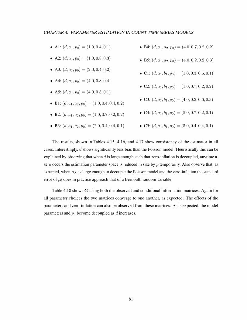
CHAPTER 4. PARAMETER ESTIMATION IN COUNT TIME SERIES MODELS
• A1: (d, a1, p0) = (1.0, 0.4, 0.1)
• A2: (d, a1, p0) = (1.0, 0.8, 0.3)
• A3: (d, a1, p0) = (2.0, 0.4, 0.2)
• A4: (d, a1, p0) = (4.0, 0.8, 0.4)
• A5: (d, a1, p0) = (4.0, 0.5, 0.1)
• B1: (d, a1, a2, p0) = (1.0, 0.4, 0.4, 0.2)
• B2: (d, a1, a2, p0) = (1.0, 0.7, 0.2, 0.2)
• B3: (d, a1, a2, p0) = (2.0, 0.4, 0.4, 0.1)
• B4: (d, a1, a2, p0) = (4.0, 0.7, 0.2, 0.2)
• B5: (d, a1, a2, p0) = (4.0, 0.2, 0.2, 0.3)
• C1: (d, a1, b1, p0) = (1.0, 0.3, 0.6, 0.1)
• C2: (d, a1, b1, p0) = (1.0, 0.7, 0.2, 0.2)
• C3: (d, a1, b1, p0) = (4.0, 0.3, 0.6, 0.3)
• C4: (d, a1, b1, p0) = (5.0, 0.7, 0.2, 0.1)
• C5: (d, a1, b1, p0) = (5.0, 0.4, 0.4, 0.1)
The results, shown in Tables 4.15, 4.16, and 4.17 show consistency of the estimator in all
cases. Interestingly, d shows significantly less bias than the Poisson model. Heuristically this can be
explained by observing that when d is large enough such that zero-inflation is decoupled, anytime a
zero occurs the estimation parameter space is reduced in size by p temporarily. Also observe that, as
expected, when µX is large enough to decouple the Poisson model and the zero-inflation the standard
error of p0 does in practice approach that of a Bernoulli random variable.
Table 4.18 shows G using both the observed and conditional information matrices. Again for
all parameter choices the two matrices converge to one another, as expected. The effects of the
parameters and zero-inflation can also be observed from these matrices. As is expected, the model
parameters and p0 become decoupled as d increases.
81

CHAPTER 4. PARAMETER ESTIMATION IN COUNT TIME SERIES MODELS
Table 4.15: CMLE results for the ZIP linear (1,0) model. For each model 1000 series of length N
were simulated. The first number in each column shows the mean of the estimator. In parenthesis are
the observed and expected standard errors.
Model N d a1 p0
A1 200 1.0163(0.1377,0.1343) 0.3848(0.0858,0.0840) 0.1477(0.0510,0.0507)
1000 1.0037(0.0591,0.0600) 0.3980(0.0366,0.0375) 0.1502(0.0230,0.0227)
A2 200 1.0141(0.1431,0.1435) 0.7844(0.0865,0.0829) 0.3022(0.0449,0.0462)
1000 1.0034(0.0648,0.0635) 0.7975(0.0386,0.0367) 0.3007(0.0206,0.0206)
A3 200 2.0159(0.2039,0.2042) 0.3941(0.0742,0.0730) 0.2001(0.0344,0.0338)
1000 2.0038(0.0936,0.0909) 0.3983(0.0326,0.0328) 0.1995(0.0152,0.0151)
A4 200 4.0094(0.2665,0.2698) 0.7953(0.0581,0.0565) 0.4021(0.0345,0.0349)
1000 3.9994(0.1110,0.1201) 0.7994(0.0239,0.0249) 0.4005(0.0153,0.0156)
A5 200 4.0439(0.3545,0.3473) 0.4925(0.0527,0.0519) 0.1003(0.0217,0.0215)
1000 4.0071(0.1542,0.1551) 0.4985(0.0232,0.0231) 0.0996(0.0099,0.0097)
Table 4.16: CMLE results for the ZIP linear (2,0) model. For each model 1000 series of length N
were simulated. The first number in each column shows the mean of the estimator. In parenthesis are
the observed and expected standard errors.
Model N d a1 a2 p0
B1 200 1.0441(0.1759,0.1754) 0.3921(0.0754,0.0740) 0.3848(0.0779,0.0735) 0.2026(0.0372,0.0370)
1000 1.0066(0.0814,0.0778) 0.3978(0.0340,0.0333) 0.3979(0.0333,0.0328) 0.2007(0.0170,0.0166)
B2 200 1.0530(0.1735,0.1666) 0.6946(0.0705,0.0690) 0.1845(0.0624,0.0625) 0.2051(0.0353,0.0355)
1000 1.0099(0.0764,0.0743) 0.6985(0.0301,0.0305) 0.1976(0.0280,0.0275) 0.2001(0.0160,0.0160)
B3 200 2.0869(0.3438,0.3198) 0.3976(0.0569,0.0544) 0.3862(0.0567,0.0535) 0.0999(0.0218,0.0221)
1000 2.0187(0.1411,0.1432) 0.3985(0.0247,0.0243) 0.3981(0.0230,0.0237) 0.1005(0.0100,0.0098)
B4 200 4.0472(0.3624,0.3516) 0.6959(0.0412,0.0405) 0.1968(0.0382,0.0367) 0.2490(0.0311,0.0308)
1000 4.0072(0.1574,0.1565) 0.6991(0.0184,0.0181) 0.2000(0.0166,0.0164) 0.2504(0.0139,0.0137)
B5 200 4.0426(0.3564,0.3472) 0.1955(0.0637,0.0621) 0.1955(0.0637,0.0621) 0.2989(0.0326,0.0328)
1000 4.0105(0.1589,0.1550) 0.1981(0.0282,0.0280) 0.1983(0.0280,0.0278) 0.2996(0.0146,0.0146)
82

CHAPTER 4. PARAMETER ESTIMATION IN COUNT TIME SERIES MODELS
Table 4.17: CMLE results for the ZIP linear (1,1) model. For each model 1000 series of length N
were simulated. The first number in each column shows the mean of the estimator. In parenthesis are
the observed and expected standard errors.
Model N d a1 b1 p0
C1 200 1.2270(0.5222,0.3573) 0.2968(0.0557,0.0502) 0.5716(0.0972,0.0747) 0.0998(0.0208,0.0214)
1000 1.0297(0.1686,0.1581) 0.3004(0.0215,0.0220) 0.5959(0.0337,0.0329) 0.0995(0.0095,0.0096)
C2 200 1.0709(0.2398,0.2146) 0.6972(0.0650,0.0639) 0.1839(0.0730,0.0689) 0.2004(0.0322,0.0333)
1000 1.0132(0.0969,0.0960) 0.6989(0.0290,0.0287) 0.1973(0.0320,0.0311) 0.1996(0.0142,0.0149)
C3 200 4.2795(1.0085,0.7634) 0.3019(0.0337,0.0311) 0.5857(0.0602,0.0484) 0.2987(0.0313,0.0324)
1000 4.0342(0.3908,0.3429) 0.3004(0.0148,0.0141) 0.5983(0.0246,0.0219) 0.2997(0.0146,0.0145)
C4 200 5.0919(0.6807,0.6478) 0.6981(0.0291,0.0285) 0.1972(0.0340,0.0334) 0.1005(0.0210,0.0211)
1000 5.0149(0.3097,0.2881) 0.7002(0.0126,0.0126) 0.1996(0.0155,0.0147) 0.0999(0.0095,0.0095)
C5 200 5.1527(1.0384,0.9116) 0.4008(0.0375,0.0362) 0.3917(0.0692,0.0622) 0.1494(0.0250,0.0253)
1000 5.0450(0.4240,0.4051) 0.3996(0.0155,0.0163) 0.3979(0.0281,0.0278) 0.1500(0.0109,0.0113)
83
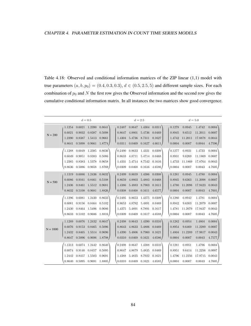
CHAPTER 4. PARAMETER ESTIMATION IN COUNT TIME SERIES MODELS
Table 4.18: Observed and conditional information matrices of the ZIP linear (1,1) model with
true parameters (a, b, p0) = (0.4, 0.3, 0.3), d ∈ (0.5, 2.5, 5) and different sample sizes. For each
combination of p0 and N the first row gives the Observed information and the second row gives the
cumulative conditional information matrix. In all instances the two matrices show good convergence.
d = 0.5 d = 2.5 d = 5.0
N = 200
1.1254 0.6021 1.2390 0.8641
0.6021 0.9032 0.8387 0.5098
1.2390 0.8387 1.5413 0.9661
0.8641 0.5098 0.9661 1.8774
0.2487 0.8647 1.4304 0.0311
0.8647 4.8801 5.4736 0.0469
1.4304 5.4736 8.7311 0.1627
0.0311 0.0469 0.1627 4.6611
0.1278 0.8945 1.4742 0.0004
0.8945 9.6512 11.2011 0.0007
1.4742 11.2011 17.8878 0.0044
0.0004 0.0007 0.0044 4.7596
1.1288 0.6049 1.2385 0.8636
0.6049 0.9051 0.8383 0.5086
1.2385 0.8383 1.5378 0.9658
0.8636 0.5086 0.9658 1.8769
0.2490 0.8633 1.4331 0.0309
0.8633 4.8711 5.4714 0.0468
1.4331 5.4714 8.7542 0.1616
0.0309 0.0468 0.1616 4.6586
0.1277 0.8931 1.4733 0.0004
0.8931 9.6269 11.1869 0.0007
1.4733 11.1869 17.8764 0.0043
0.0004 0.0007 0.0043 4.7605
N = 500
1.1319 0.6086 1.2436 0.8632
0.6086 0.9161 0.8461 0.5108
1.2436 0.8461 1.5512 0.9681
0.8632 0.5108 0.9681 1.8826
0.2499 0.8659 1.4386 0.0308
0.8659 4.8803 5.4883 0.0468
1.4386 5.4883 8.7903 0.1611
0.0308 0.0468 0.1611 4.6577
0.1281 0.8945 1.4780 0.0004
0.8945 9.6363 11.2098 0.0007
1.4780 11.2098 17.9423 0.0043
0.0004 0.0007 0.0043 4.7601
1.1296 0.6081 1.2430 0.8633
0.6081 0.9156 0.8464 0.5102
1.2430 0.8464 1.5496 0.9686
0.8633 0.5102 0.9686 1.8816
0.2495 0.8653 1.4375 0.0309
0.8653 4.8792 5.4891 0.0469
1.4375 5.4891 8.7891 0.1617
0.0309 0.0469 0.1617 4.6588
0.1280 0.8942 1.4781 0.0004
0.8942 9.6303 11.2079 0.0007
1.4781 11.2079 17.9437 0.0043
0.0004 0.0007 0.0043 4.7605
N = 1000
1.1289 0.6076 1.2432 0.8647
0.6076 0.9153 0.8465 0.5096
1.2432 0.8465 1.5514 0.9696
0.8647 0.5096 0.9696 1.8798
0.2498 0.8643 1.4390 0.0310
0.8643 4.8633 5.4806 0.0469
1.4390 5.4806 8.7960 0.1621
0.0310 0.0469 0.1621 4.6586
0.1282 0.8954 1.4804 0.0004
0.8954 9.6469 11.2289 0.0007
1.4804 11.2289 17.9817 0.0043
0.0004 0.0007 0.0043 4.7577
1.1313 0.6074 1.2442 0.8640
0.6074 0.9140 0.8457 0.5095
1.2442 0.8457 1.5503 0.9691
0.8640 0.5095 0.9691 1.8805
0.2498 0.8647 1.4388 0.0310
0.8647 4.8679 5.4835 0.0469
1.4388 5.4835 8.7922 0.1621
0.0310 0.0469 0.1621 4.6585
0.1281 0.8951 1.4796 0.0004
0.8951 9.6414 11.2256 0.0007
1.4796 11.2256 17.9715 0.0043
0.0004 0.0007 0.0043 4.7605
84

CHAPTER 4. PARAMETER ESTIMATION IN COUNT TIME SERIES MODELS
4.6 Linear Zero-Inflated Negative Binomial Estimation
CMLE estimation of the ZINB2 linear model follows the steps laid out in previous sections.
The conditional likelihood function of the ZINB2 model is given by (4.55) and the CLL is given by
(4.56).
L (p0, ν,θ) =∏xn=0
(p0 +
(ν
λn + ν
)ν)∏xn 6=0
(1− p0)
(Γ (xn + ν)
Γ (ν) Γ (xn + 1)
(ν
λn + ν
)ν)( λnλn + ν
)xn(4.55)
L (p0, ν,θ) =∑xn=0
log
(p0 +
(ν
λn + ν
)ν)+∑xn 6=0
log (1− p0) + ln Γ (xn + ν)− ln Γ (xn + 1)− ln Γ (ν)
+ ν [ln ν − ln (λn + ν)] + xn [lnλn − ln (λn + ν)] (4.56)
Taking derivatives of (4.56) yields the score vector. Note that h(p0, ν,θ) and all of its derivatives are
given in Appendix B.
∂L (p0, ν,θ)
∂p0=∂h(p0, ν,θ)
∂p0
/h(p0, ν,θ) (4.57a)
∂L (p0, ν,θ)
∂ν=∂h(p0, ν,θ)
∂ν
/h(p0, ν,θ) (4.57b)
∂L (p0, ν,θ)
∂θ=∂h(p0, ν,θ)
∂θ
/h(p0, ν,θ) (4.57c)
Further differentiation of the score vector yieldsHn (θ).
∂2L (p0, ν,θ)
∂p20
=
(∂2h(p0, ν,θ)
∂p20
−(∂h(p0, ν,θ)
∂p0
)2)/
h(p0, ν,θ)2 (4.58a)
∂2L (p0, ν,θ)
∂ν2=
(∂2h(p0, ν,θ)
∂ν2−(∂h(p0, ν,θ)
∂ν
)2)/
h(p0, ν,θ)2 (4.58b)
∂2L (p0, ν,θ)
∂θ∂θT=
(∂2h(p0, ν,θ)
∂θ∂θT−(∂h(p0, ν,θ)
∂θ
)(∂h(p0, ν,θ)
∂θ
)′)/h(p0, ν,θ)2 (4.58c)
∂2L (p0, ν,θ)
∂p0∂ν=
(∂2h(p0, ν,θ)
∂p0∂ν− ∂h(p0, ν,θ)
∂p0
∂h(p0, ν,θ)
∂ν
)/h(p0, ν,θ)2 (4.58d)
∂2L (p0, ν,θ)
∂p0∂θ=
(∂2h(p0, ν,θ)
∂p0∂θ− ∂h(p0, ν,θ)
∂p0
∂h(p0, ν,θ)
∂θ
)/h(p0, ν,θ)2 (4.58e)
∂2L (p0, ν,θ)
∂ν∂θ=
(∂2h(p0, ν,θ)
∂ν∂θ− ∂h(p0, ν,θ)
∂ν
∂h(p0, ν,θ)
∂θ
)/h(p0, ν,θ)2 (4.58f)
85

CHAPTER 4. PARAMETER ESTIMATION IN COUNT TIME SERIES MODELS
The logic of Sections 4.4 and 4.5 implies that equivalence of −Hn (θ) and Gn (θ) relies on the
same assumptions as those made for the NB2 model.
A simulation study identical in methodology to the previous sections was also performed for
the ZINB2 linear model. The parameters sets, given below, were chosen to span a wide range of
possible models.
• A1: (d, a1, ν, p0) = (1.0, 0.4, 2.0, 0.1)
• A2: (d, a1, ν, p0) = (1.0, 0.8, 3.0, 0.3)
• A3: (d, a1, ν, p0) = (2.0, 0.4, 5.0, 0.2)
• A4: (d, a1, ν, p0) = (4.0, 0.8, 2.0, 0.4)
• A5: (d, a1, ν, p0) = (4.0, 0.5, 5.0, 0.1)
• B1: (d, a1, a2, ν, p0) = (1.0, 0.4, 0.4, 2.0, 0.2)
• B2: (d, a1, a2, ν, p0) = (1.0, 0.7, 0.2, 5.0, 0.2)
• B3: (d, a1, a2, ν, p0) = (2.0, 0.4, 0.4, 2.0, 0.1)
• B4: (d, a1, a2, ν, p0) = (4.0, 0.7, 0.2, 5.0, 0.2)
• B5: (d, a1, a2, ν, p0) = (4.0, 0.2, 0.2, 5.0, 0.3)
• C1: (d, a1, b1, ν, p0) = (1.0, 0.3, 0.6, 2.0, 0.1)
• C2: (d, a1, b1, ν, p0) = (1.0, 0.7, 0.2, 5.0, 0.2)
• C3: (d, a1, b1, ν, p0) = (4.0, 0.3, 0.6, 2.0, 0.3)
• C4: (d, a1, b1, ν, p0) = (5.0, 0.7, 0.2, 5.0, 0.1)
• C5: (d, a1, b1, ν, p0) = (5.0, 0.4, 0.4, 5.0, 0.1)
The results, shown in Tables 4.8 through 4.10, show that the estimators are consistent with the
caveat that, similar to the NB2 model, shorter series with larger dispersion parameters sometimes
appear to be Poisson, biasing ν. Similar to the ZIP model when θ is such that the probability of the
underlying NB2 distribution generating a 0 is small the standard error on p0 approaches that of a
Bernoulli random variable.
Table 4.22 again shows convergence of the two estimators forG. Similar to the ZIP decoupling
of the zero-inflation parameter and the NB2 distribution can be observed in these matrices. There
would likely be a greater decoupling of ν and p0 for a larger value of ν.
86

CHAPTER 4. PARAMETER ESTIMATION IN COUNT TIME SERIES MODELS
Table 4.19: CMLE results for the ZINB2 linear (1,0) model. For each model 1000 series of length N
were simulated. The first number in each column shows the mean of the estimator. In parenthesis are
the observed and expected standard errors.
Model N d a1 ν p0
A1 200 1.0175(0.1781,0.1941) 0.3934(0.1143,0.1143) 2.4830(1.3363,1.1412) 0.1443(0.0946,0.1167)
1000 1.0042(0.0860,0.0864) 0.3957(0.0506,0.0514) 2.0913(0.5495,0.5127) 0.1462(0.0517,0.0523)
A2 200 1.0097(0.1738,0.1716) 0.7782(0.1355,0.1338) 3.5042(1.7003,1.4117) 0.2937(0.0668,0.0651)
1000 1.0031(0.0743,0.0756) 0.7960(0.0611,0.0596) 3.1148(0.6546,0.6214) 0.2997(0.0286,0.0287)
A3 200 2.0294(0.2530,0.2376) 0.3884(0.0909,0.0878) 5.8988(2.5170,2.0632) 0.1974(0.0450,0.0429)
1000 1.9992(0.1067,0.1065) 0.3992(0.0400,0.0394) 5.2303(1.0866,0.9494) 0.2002(0.0195,0.0194)
A4 200 4.0137(0.4676,0.4823) 0.7821(0.1465,0.1524) 2.1399(0.5427,0.4663) 0.3997(0.0408,0.0403)
1000 3.9922(0.2199,0.2151) 0.8007(0.0681,0.0679) 2.0240(0.2054,0.2060) 0.3995(0.0179,0.0180)
A5 200 4.0620(0.4191,0.4225) 0.4907(0.0695,0.0703) 5.3381(1.1776,1.0087) 0.0993(0.0237,0.0234)
1000 4.0283(0.1859,0.1887) 0.4946(0.0321,0.0316) 5.0367(0.4633,0.4590) 0.1003(0.0105,0.0105)
Table 4.20: CMLE results for the ZINB2 linear (2,0) model. For each model 1000 series of length N
were simulated. The first number in each column shows the mean of the estimator. In parenthesis are
the observed and expected standard errors.
Model N d a1 a2 ν p0
B1 200 1.0328(0.2026,0.2056) 0.3947(0.1143,0.1095) 0.3828(0.1141,0.1096) 2.3069(0.9280,0.7224) 0.1992(0.0644,0.0643)
1000 1.0085(0.0910,0.0904) 0.3982(0.0488,0.0487) 0.3935(0.0488,0.0487) 2.0542(0.3237,0.3001) 0.1983(0.0283,0.0279)
B2 200 1.0302(0.1878,0.1837) 0.6928(0.0973,0.0935) 0.1896(0.0747,0.0722) 6.0299(2.8690,1.8971) 0.2014(0.0455,0.0426)
1000 1.0052(0.0795,0.0813) 0.6982(0.0429,0.0419) 0.1975(0.0332,0.0326) 5.2055(0.8575,0.7843) 0.2006(0.0186,0.0188)
B3 200 2.1157(0.4214,0.3910) 0.3896(0.0866,0.0900) 0.3805(0.0861,0.0895) 2.1157(0.4254,0.3946) 0.1020(0.0342,0.0327)
1000 2.0102(0.1754,0.1742) 0.3984(0.0410,0.0400) 0.3983(0.0400,0.0396) 2.0192(0.1730,0.1690) 0.0996(0.0145,0.0146)
B4 200 4.0659(0.5305,0.4985) 0.6957(0.0808,0.0781) 0.1935(0.0592,0.0589) 5.2774(1.1324,0.9564) 0.2498(0.0323,0.0315)
1000 4.0093(0.2307,0.2229) 0.6991(0.0356,0.0347) 0.2000(0.0253,0.0261) 5.0622(0.4279,0.4173) 0.2494(0.0142,0.0141)
B5 200 4.0788(0.4642,0.4514) 0.1940(0.0838,0.0832) 0.1862(0.0850,0.0830) 5.6289(1.8084,1.3765) 0.2996(0.0361,0.0345)
1000 4.0025(0.2005,0.2012) 0.2003(0.0377,0.0371) 0.1990(0.0378,0.0369) 5.1150(0.6609,0.6087) 0.2995(0.0152,0.0154)
Table 4.21: CMLE results for the ZINB2 linear (1,1) model. For each model 1000 series of length N
were simulated. The first number in each column shows the mean of the estimator. In parenthesis are
the observed and expected standard errors.
Model N d a1 b1 ν p0
C1 200 1.2936(0.6467,0.4742) 0.2982(0.0796,0.0771) 0.5570(0.1281,0.1046) 2.1015(0.3798,0.3577) 0.1007(0.0305,0.0299)
1000 1.0608(0.2218,0.2079) 0.2996(0.0355,0.0345) 0.5916(0.0481,0.0460) 2.0154(0.1615,0.1588) 0.0997(0.0136,0.0133)
C2 200 1.0719(0.2536,0.2436) 0.6874(0.0947,0.0888) 0.1889(0.0857,0.0815) 5.9016(2.4593,1.6384) 0.2012(0.0391,0.0386)
1000 1.0182(0.1090,0.1085) 0.6995(0.0409,0.0401) 0.1949(0.0367,0.0365) 5.1656(0.7679,0.7168) 0.2009(0.0173,0.0173)
C3 200 5.0708(2.5186,1.7822) 0.3059(0.0928,0.0863) 0.5422(0.1521,0.1189) 2.0745(0.3059,0.2873) 0.2987(0.0334,0.0331)
1000 4.1221(0.8750,0.8127) 0.2987(0.0400,0.0393) 0.5943(0.0574,0.0543) 2.0203(0.1310,0.1270) 0.2988(0.0142,0.0148)
C4 200 5.3407(1.1377,1.0487) 0.6944(0.0626,0.0631) 0.1873(0.0623,0.0590) 5.1297(0.6981,0.6845) 0.1011(0.0214,0.0213)
1000 5.0413(0.5014,0.4660) 0.7001(0.0291,0.0278) 0.1981(0.0264,0.0258) 5.0100(0.2997,0.2964) 0.0999(0.0095,0.0095)
C5 200 5.3617(1.7277,1.4770) 0.3937(0.0692,0.0658) 0.3854(0.1177,0.1034) 5.1964(0.8060,0.7101) 0.1500(0.0248,0.0253)
1000 5.0315(0.6687,0.6499) 0.3982(0.0292,0.0293) 0.3993(0.0457,0.0455) 5.0325(0.3147,0.3161) 0.1499(0.0113,0.0113)
87

CHAPTER 4. PARAMETER ESTIMATION IN COUNT TIME SERIES MODELS
Table 4.22: Observed and conditional information matrices of the ZINB2 linear (1,1) model with
true parameters (a, b, ν, p0) = (0.4, 0.4, 2, 0.15), d ∈ (0.5, 2.5, 5) and different sample sizes. For
each combination of p0 and N the first row shows the Observed information and the second row
shows an estimate of the expected information via the cumulative conditional information matrix.
We observe that in all instances the two matrices show good convergence.
d = 0.5 d = 2.5 d = 5.0
N = 200
0.8477 0.6882 1.3134 −0.0124 −0.6705
0.6882 1.3615 1.4347 −0.0222 −0.7083
1.3134 1.4347 2.4430 −0.0245 −1.1236
−0.0124 −0.0222 −0.0245 0.0164 −0.1114
−0.6705 −0.7083 −1.1236 −0.1114 2.2230
0.0588 0.2766 0.4768 −0.0069 −0.0785
0.2766 2.3023 2.6850 −0.0368 −0.3398
0.4768 2.6850 4.3512 −0.0576 −0.6230
−0.0069 −0.0368 −0.0576 0.0503 −0.1630
−0.0785 −0.3398 −0.6230 −0.1630 6.2100
0.0168 0.1608 0.2742 −0.0025 −0.0162
0.1608 2.6071 3.0909 −0.0229 −0.1333
0.2742 3.0909 4.9863 −0.0401 −0.2543
−0.0025 −0.0229 −0.0401 0.0726 −0.0949
−0.0162 −0.1333 −0.2543 −0.0949 7.2016
0.8407 0.6835 1.3047 −0.0115 −0.6741
0.6835 1.3620 1.4316 −0.0218 −0.7132
1.3047 1.4316 2.4342 −0.0229 −1.1287
−0.0115 −0.0218 −0.0229 0.0165 −0.1115
−0.6741 −0.7132 −1.1287 −0.1115 2.2230
0.0589 0.2778 0.4765 −0.0071 −0.0778
0.2778 2.3165 2.6927 −0.0381 −0.3377
0.4765 2.6927 4.3479 −0.0587 −0.6165
−0.0071 −0.0381 −0.0587 0.0513 −0.1620
−0.0778 −0.3377 −0.6165 −0.1620 6.2100
0.0169 0.1618 0.2760 −0.0026 −0.0164
0.1618 2.6213 3.1120 −0.0261 −0.1339
0.2760 3.1120 5.0254 −0.0436 −0.2566
−0.0026 −0.0261 −0.0436 0.0744 −0.0937
−0.0164 −0.1339 −0.2566 −0.0937 7.2016
N = 500
0.8524 0.6834 1.3176 −0.0119 −0.6748
0.6834 1.3454 1.4261 −0.0211 −0.7088
1.3176 1.4261 2.4428 −0.0234 −1.1294
−0.0119 −0.0211 −0.0234 0.0162 −0.1113
−0.6748 −0.7088 −1.1294 −0.1113 2.2182
0.0591 0.2796 0.4796 −0.0072 −0.0781
0.2796 2.3349 2.7190 −0.0370 −0.3375
0.4796 2.7190 4.3905 −0.0603 −0.6194
−0.0072 −0.0370 −0.0603 0.0510 −0.1617
−0.0781 −0.3375 −0.6194 −0.1617 6.1712
0.0169 0.1609 0.2747 −0.0024 −0.0164
0.1609 2.6003 3.0932 −0.0217 −0.1336
0.2747 3.0932 5.0003 −0.0384 −0.2562
−0.0024 −0.0217 −0.0384 0.0727 −0.0951
−0.0164 −0.1336 −0.2562 −0.0951 7.2074
0.8496 0.6831 1.3177 −0.0118 −0.6762
0.6831 1.3420 1.4244 −0.0210 −0.7089
1.3177 1.4244 2.4496 −0.0235 −1.1299
−0.0118 −0.0210 −0.0235 0.0162 −0.1115
−0.6762 −0.7089 −1.1299 −0.1115 2.2182
0.0591 0.2798 0.4804 −0.0073 −0.0784
0.2798 2.3411 2.7297 −0.0386 −0.3371
0.4804 2.7297 4.4101 −0.0625 −0.6225
−0.0073 −0.0386 −0.0625 0.0513 −0.1618
−0.0784 −0.3371 −0.6225 −0.1618 6.1712
0.0169 0.1611 0.2751 −0.0026 −0.0163
0.1611 2.5954 3.0869 −0.0227 −0.1308
0.2751 3.0869 4.9961 −0.0415 −0.2533
−0.0026 −0.0227 −0.0415 0.0728 −0.0954
−0.0163 −0.1308 −0.2533 −0.0954 7.2074
N = 1000
0.8488 0.6776 1.3162 −0.0112 −0.6800
0.6776 1.3325 1.4194 −0.0202 −0.7052
1.3162 1.4194 2.4467 −0.0225 −1.1308
−0.0112 −0.0202 −0.0225 0.0161 −0.1109
−0.6800 −0.7052 −1.1308 −0.1109 2.2060
0.0592 0.2780 0.4794 −0.0070 −0.0787
0.2780 2.3094 2.7019 −0.0359 −0.3392
0.4794 2.7019 4.3844 −0.0579 −0.6232
−0.0070 −0.0359 −0.0579 0.0505 −0.1626
−0.0787 −0.3392 −0.6232 −0.1626 6.1931
0.0169 0.1612 0.2748 −0.0025 −0.0166
0.1612 2.6138 3.0975 −0.0238 −0.1348
0.2748 3.0975 4.9966 −0.0407 −0.2594
−0.0025 −0.0238 −0.0407 0.0724 −0.0960
−0.0166 −0.1348 −0.2594 −0.0960 7.2509
0.8497 0.6770 1.3125 −0.0114 −0.6767
0.6770 1.3296 1.4128 −0.0207 −0.7021
1.3125 1.4128 2.4343 −0.0230 −1.1258
−0.0114 −0.0207 −0.0230 0.0162 −0.1111
−0.6767 −0.7021 −1.1258 −0.1111 2.2060
0.0594 0.2787 0.4806 −0.0072 −0.0781
0.2787 2.3097 2.7021 −0.0367 −0.3351
0.4806 2.7021 4.3836 −0.0600 −0.6180
−0.0072 −0.0367 −0.0600 0.0508 −0.1624
−0.0781 −0.3351 −0.6180 −0.1624 6.1931
0.0169 0.1618 0.2754 −0.0025 −0.0167
0.1618 2.6303 3.1169 −0.0254 −0.1370
0.2754 3.1169 5.0224 −0.0415 −0.2612
−0.0025 −0.0254 −0.0415 0.0727 −0.0954
−0.0167 −0.1370 −0.2612 −0.0954 7.2509
88
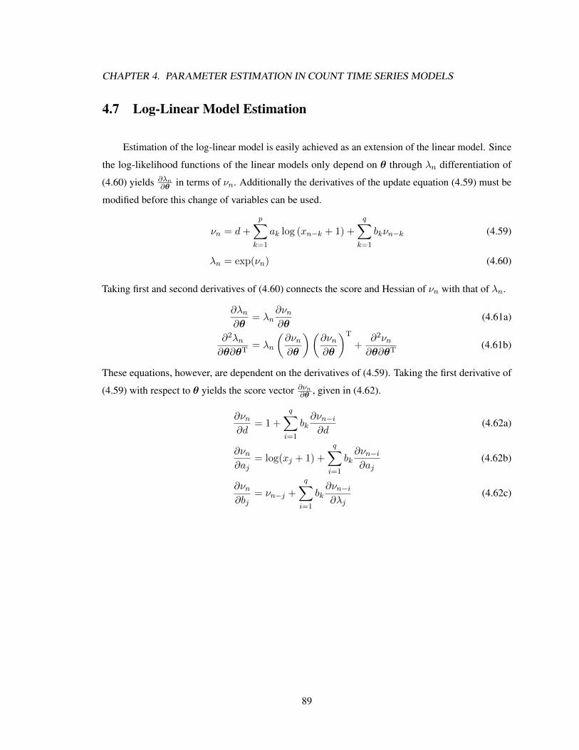
CHAPTER 4. PARAMETER ESTIMATION IN COUNT TIME SERIES MODELS
4.7 Log-Linear Model Estimation
Estimation of the log-linear model is easily achieved as an extension of the linear model. Since
the log-likelihood functions of the linear models only depend on θ through λn differentiation of
(4.60) yields ∂λn∂θ in terms of νn. Additionally the derivatives of the update equation (4.59) must be
modified before this change of variables can be used.
νn = d+
p∑k=1
ak log (xn−k + 1) +
q∑k=1
bkνn−k (4.59)
λn = exp(νn) (4.60)
Taking first and second derivatives of (4.60) connects the score and Hessian of νn with that of λn.
∂λn∂θ
= λn∂νn∂θ
(4.61a)
∂2λn∂θ∂θT
= λn
(∂νn∂θ
)(∂νn∂θ
)T
+∂2νn∂θ∂θT
(4.61b)
These equations, however, are dependent on the derivatives of (4.59). Taking the first derivative of
(4.59) with respect to θ yields the score vector ∂νn∂θ , given in (4.62).
∂νn∂d
= 1 +
q∑i=1
bk∂νn−i∂d
(4.62a)
∂νn∂aj
= log(xj + 1) +
q∑i=1
bk∂νn−i∂aj
(4.62b)
∂νn∂bj
= νn−j +
q∑i=1
bk∂νn−i∂λj
(4.62c)
89

CHAPTER 4. PARAMETER ESTIMATION IN COUNT TIME SERIES MODELS
Similarly taking derivatives of ∂νn∂θ with respect to θ yields the Hessian of νn, ∂2νn∂θ∂θT , given in (4.63).
∂2νn∂d2
=
q∑i=1
bk∂2νn−i∂d2
(4.63a)
∂2νn∂d∂aj
=
q∑i=1
bk∂2νn−j∂d∂aj
(4.63b)
∂2νn∂d∂bj
=∂νn−j∂d
+
q∑i=1
bk∂2νn−i∂d∂bj
(4.63c)
∂2νn∂aj∂ak
=
q∑i=1
bk∂2νn−i∂aj∂ak
(4.63d)
∂2νn∂bj∂bk
=∂νn−j∂bk
+∂νn−k∂bj
+
q∑i=1
bk∂2νn−i∂bj∂bk
(4.63e)
∂2νn∂aj∂bk
=∂νn−k∂aj
+
q∑i=1
bk∂2νn−i∂aj∂bk
(4.63f)
Conveniently (4.61a) and (4.61b) are deterministic conditioned on In−1 allowing them to be
substituted into equations for Sn (θ), Hn (θ), their expected values, and Gn (θ). This allows the
results of sections 4.3 through 4.6 to be easily adapted to the log-linear models. Below we apply
(4.61a) and (4.61b) to the linear models ans give the results of Monte Carlo simulations performed
to assess the CMLE for the log-linear models.
For the Poisson model (4.11), (4.12), and (4.18) become
∂L (θ)
∂θ=
N∑n=0
(xn − λn)∂νn∂θ
(4.64)
∂2L (θ)
∂θ∂θT=
N∑n=0
λn
(∂νn∂θ
)(∂νn∂θ
)T
− (xn − λn)∂2νn∂θ∂θT
(4.65)
G = E
[λn
(∂νn∂θ
)(∂νn∂θ
)T]
(4.66)
We performed a simulation study identical (except for the model parameters) to the one described
in Section 4.3 was performed. The parameter sets, given below, were chosen to include a wide range
of possibilities.
90

CHAPTER 4. PARAMETER ESTIMATION IN COUNT TIME SERIES MODELS
Table 4.23: CMLE results for the Poisson log-linear (1,0) model. For each model 1000 series of
length N were simulated. The first number in each column shows the mean of the estimator. In
parenthesis are the observed and expected standard errors.
Model N d a1
A1 200 2.0416(0.2250,0.2255) 0.3875(0.0664,0.0666)
1000 2.0074(0.0983,0.1007) 0.3978(0.0290,0.0297)
A2 200 2.9931(0.1346,0.1387) -0.3972(0.0620,0.0640)
1000 2.9998(0.0621,0.0619) -0.3999(0.0286,0.0286)
A3 200 2.9928(0.0750,0.0727) -0.7947(0.0485,0.0462)
1000 2.9976(0.0331,0.0322) -0.7986(0.0207,0.0205)
A4 200 4.9962(0.1953,0.2016) -0.4988(0.0588,0.0606)
1000 4.9978(0.0906,0.0904) -0.4993(0.0272,0.0271)
A5 200 4.9773(0.1144,0.1104) -0.7919(0.0421,0.0409)
1000 4.9963(0.0482,0.0492) -0.7986(0.0179,0.0183)
• A1: (d, a1) = (2.0, 0.4)
• A2: (d, a1) = (3.0,−0.4)
• A3: (d, a1) = (3.0,−0.8)
• A4: (d, a1) = (5.0,−0.5)
• A5: (d, a1) = (5.0,−0.8)
• B1: (d, a1, a2) = (5.0,−0.4,−0.4)
• B2: (d, a1, a2) = (4.0,−0.7, 0.2)
• B3: (d, a1, a2) = (2.0,−0.4, 0.7)
• B4: (d, a1, a2) = (5.0,−0.2,−0.2)
• B5: (d, a1, a2) = (2.0, 0.2, 0.2)
• C1: (d, a1, b1) = (3.0,−0.3,−0.6)
• C2: (d, a1, b1) = (3.0,−0.7, 0.2)
• C3: (d, a1, b1) = (3.0, 0.3,−0.6)
• C4: (d, a1, b1) = (5.0,−0.7, 0.2)
• C5: (d, a1, b1) = (5.0,−0.4,−0.4)
The results, shown in Tables 4.23 through 4.25 appear to be consistent for most models.
Anomalous behavior occurs for models B3 and C4. The cause of the anomalous behavior for model
B3 can be attributed to the fact that the parameters are actually outside the region of stationarity.
Comparing these results to C2 and C4, where the only difference is d, suggest that perhaps model C4
is not stationary as well. Table 4.26 shows estimators ofG based on the observed and conditional
information matrices. In each case the matrices appear to be consistent with one another, as expected.
91
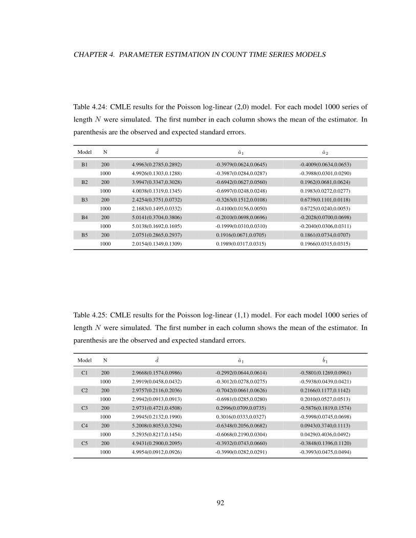
CHAPTER 4. PARAMETER ESTIMATION IN COUNT TIME SERIES MODELS
Table 4.24: CMLE results for the Poisson log-linear (2,0) model. For each model 1000 series of
length N were simulated. The first number in each column shows the mean of the estimator. In
parenthesis are the observed and expected standard errors.
Model N d a1 a2
B1 200 4.9963(0.2785,0.2892) -0.3979(0.0624,0.0645) -0.4009(0.0634,0.0653)
1000 4.9926(0.1303,0.1288) -0.3987(0.0284,0.0287) -0.3988(0.0301,0.0290)
B2 200 3.9947(0.3347,0.3028) -0.6942(0.0627,0.0560) 0.1962(0.0681,0.0624)
1000 4.0038(0.1319,0.1345) -0.6997(0.0248,0.0248) 0.1983(0.0272,0.0277)
B3 200 2.4254(0.3751,0.0732) -0.3263(0.1512,0.0108) 0.6739(0.1101,0.0118)
1000 2.1683(0.1495,0.0332) -0.4100(0.0156,0.0050) 0.6725(0.0240,0.0053)
B4 200 5.0141(0.3704,0.3806) -0.2010(0.0698,0.0696) -0.2028(0.0700,0.0698)
1000 5.0138(0.1692,0.1695) -0.1999(0.0310,0.0310) -0.2040(0.0306,0.0311)
B5 200 2.0751(0.2865,0.2937) 0.1916(0.0671,0.0705) 0.1861(0.0734,0.0707)
1000 2.0154(0.1349,0.1309) 0.1989(0.0317,0.0315) 0.1966(0.0315,0.0315)
Table 4.25: CMLE results for the Poisson log-linear (1,1) model. For each model 1000 series of
length N were simulated. The first number in each column shows the mean of the estimator. In
parenthesis are the observed and expected standard errors.
Model N d a1 b1
C1 200 2.9668(0.1574,0.0986) -0.2992(0.0644,0.0614) -0.5801(0.1269,0.0961)
1000 2.9919(0.0458,0.0432) -0.3012(0.0278,0.0275) -0.5938(0.0439,0.0421)
C2 200 2.9757(0.2116,0.2036) -0.7042(0.0661,0.0626) 0.2166(0.1177,0.1142)
1000 2.9942(0.0913,0.0913) -0.6981(0.0285,0.0280) 0.2010(0.0527,0.0513)
C3 200 2.9731(0.4721,0.4508) 0.2996(0.0709,0.0735) -0.5876(0.1819,0.1574)
1000 2.9945(0.2132,0.1990) 0.3016(0.0333,0.0327) -0.5998(0.0745,0.0698)
C4 200 5.2008(0.8053,0.3294) -0.6348(0.2056,0.0682) 0.0943(0.3740,0.1113)
1000 5.2935(0.8217,0.1454) -0.6068(0.2190,0.0304) 0.0429(0.4036,0.0492)
C5 200 4.9431(0.2900,0.2095) -0.3932(0.0743,0.0660) -0.3848(0.1396,0.1120)
1000 4.9954(0.0912,0.0926) -0.3990(0.0282,0.0291) -0.3993(0.0475,0.0494)
92
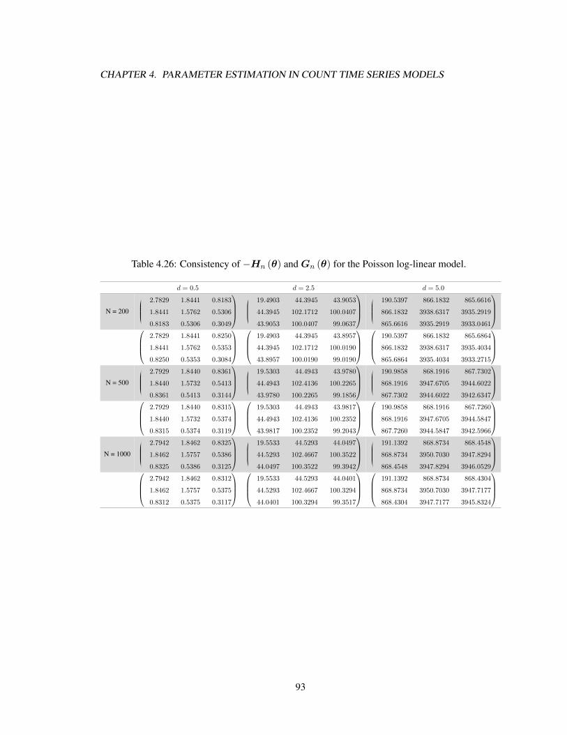
CHAPTER 4. PARAMETER ESTIMATION IN COUNT TIME SERIES MODELS
Table 4.26: Consistency of −Hn (θ) andGn (θ) for the Poisson log-linear model.
d = 0.5 d = 2.5 d = 5.0
N = 200
2.7829 1.8441 0.8183
1.8441 1.5762 0.5306
0.8183 0.5306 0.3049
19.4903 44.3945 43.9053
44.3945 102.1712 100.0407
43.9053 100.0407 99.0637
190.5397 866.1832 865.6616
866.1832 3938.6317 3935.2919
865.6616 3935.2919 3933.0461
2.7829 1.8441 0.8250
1.8441 1.5762 0.5353
0.8250 0.5353 0.3084
19.4903 44.3945 43.8957
44.3945 102.1712 100.0190
43.8957 100.0190 99.0190
190.5397 866.1832 865.6864
866.1832 3938.6317 3935.4034
865.6864 3935.4034 3933.2715
N = 500
2.7929 1.8440 0.8361
1.8440 1.5732 0.5413
0.8361 0.5413 0.3144
19.5303 44.4943 43.9780
44.4943 102.4136 100.2265
43.9780 100.2265 99.1856
190.9858 868.1916 867.7302
868.1916 3947.6705 3944.6022
867.7302 3944.6022 3942.6347
2.7929 1.8440 0.8315
1.8440 1.5732 0.5374
0.8315 0.5374 0.3119
19.5303 44.4943 43.9817
44.4943 102.4136 100.2352
43.9817 100.2352 99.2043
190.9858 868.1916 867.7260
868.1916 3947.6705 3944.5847
867.7260 3944.5847 3942.5966
N = 1000
2.7942 1.8462 0.8325
1.8462 1.5757 0.5386
0.8325 0.5386 0.3125
19.5533 44.5293 44.0497
44.5293 102.4667 100.3522
44.0497 100.3522 99.3942
191.1392 868.8734 868.4548
868.8734 3950.7030 3947.8294
868.4548 3947.8294 3946.0529
2.7942 1.8462 0.8312
1.8462 1.5757 0.5375
0.8312 0.5375 0.3117
19.5533 44.5293 44.0401
44.5293 102.4667 100.3294
44.0401 100.3294 99.3517
191.1392 868.8734 868.4304
868.8734 3950.7030 3947.7177
868.4304 3947.7177 3945.8324
93

CHAPTER 4. PARAMETER ESTIMATION IN COUNT TIME SERIES MODELS
For the NB2 model the components of the score vector become
∂L (θ, φ)
∂ν=
N∑n=0
Ψ (λn + ν)−Ψ (ν) + ln ν − ln(λn + ν) + 1− (ν + xn)
λn + ν(4.67a)
∂L (θ, φ)
∂θ=
N∑n=0
ν(xn − λn)
(λn + ν)
∂νn∂θ
(4.67b)
and similarly the components of the Hessian become
∂2L (θ, φ)
∂ν2=
N∑n=0
Ψ′ (xn + ν)−Ψ′ (ν) +xnν + λ2
n
ν (λn + ν)2 (4.68a)
∂2L (θ, φ)
∂θ∂θT=
N∑n=0
ν(xn − λn)
(λn + ν)
∂2νn∂θ∂θT
− ν(λnν + λnxn)
(λn + ν)2
(∂νn∂θ
)(∂νn∂θ
)T
(4.68b)
∂2L (θ, φ)
∂ν∂θ= λn
(xn − λn)
(λn + ν)2
∂νn∂θ
(4.68c)
A simulation study identical to that for the Poisson log-linear model except for the inclusion of
the dispersion parameter was conducted for the NB2 model. The purpose of keeping all parameters
the same was to observe how the change in distribution affected estimation.
• A1: (d, a1, ν) = (2.0, 0.4, 2.0)
• A2: (d, a1, ν) = (3.0,−0.4, 3.0)
• A3: (d, a1, ν) = (3.0,−0.8, 5.0)
• A4: (d, a1, ν) = (5.0,−0.5, 2.0)
• A5: (d, a1, ν) = (5.0,−0.8, 5.0)
• B1: (d, a1, a2, ν) = (5.0,−0.4,−0.4, 2.0)
• B2: (d, a1, a2, ν) = (4.0,−0.7, 0.2, 5.0)
• B3: (d, a1, a2, ν) = (2.0,−0.4, 0.7, 2.0)
• B4: (d, a1, a2, ν) = (5.0,−0.2,−0.2, 5.0)
• B5: (d, a1, a2, ν) = (2.0, 0.2, 0.2, 5.0)
• C1: (d, a1, b1, ν) = (3.0,−0.3,−0.6, 2.0)
• C2: (d, a1, b1, ν) = (3.0,−0.7, 0.2, 5.0)
• C3: (d, a1, b1, ν) = (3.0, 0.3,−0.6, 2.0)
• C4: (d, a1, b1, ν) = (5.0,−0.7, 0.2, 5.0)
• C5: (d, a1, b1, ν) = (5.0,−0.4,−0.4, 5.0)
Tables 4.27 through 4.29 give the results of CMLE estimation for the log-linear NB2 model,
and Tables 4.30, through 4.32 show the results of QMLE estimation. Thereare several interesting
results from these tables. First, it appears that the estimators for models B3 and C4 are better. In fact
94
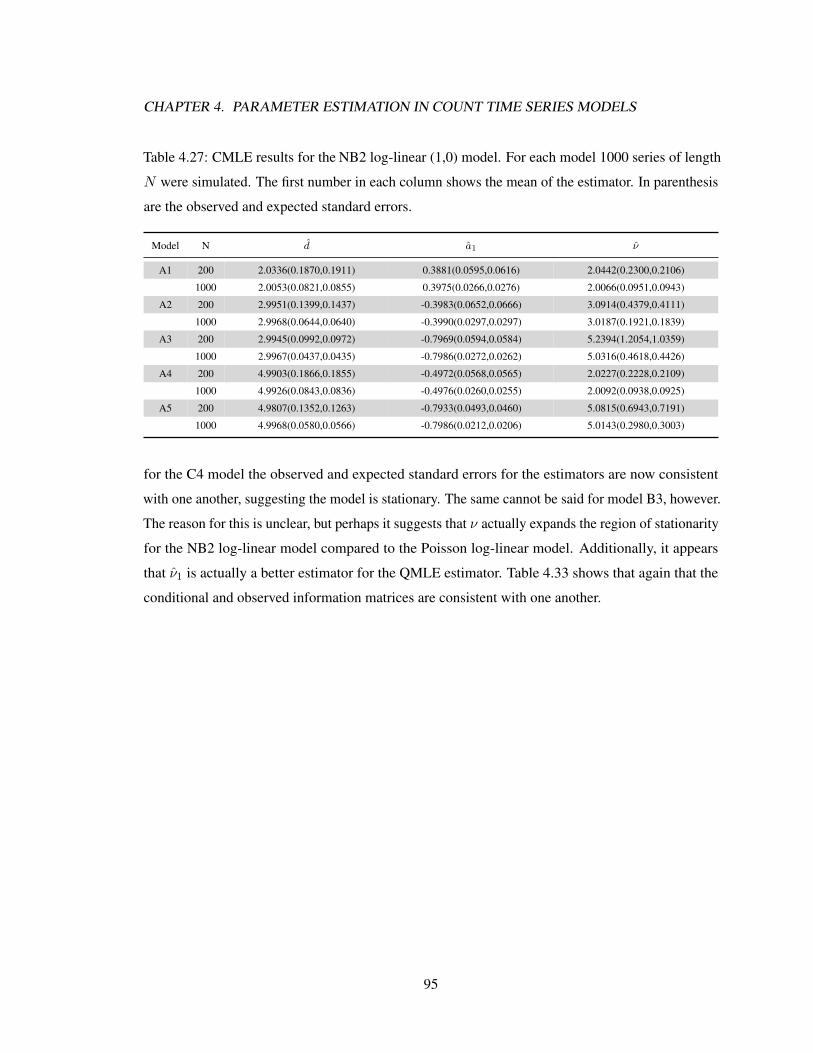
CHAPTER 4. PARAMETER ESTIMATION IN COUNT TIME SERIES MODELS
Table 4.27: CMLE results for the NB2 log-linear (1,0) model. For each model 1000 series of length
N were simulated. The first number in each column shows the mean of the estimator. In parenthesis
are the observed and expected standard errors.
Model N d a1 ν
A1 200 2.0336(0.1870,0.1911) 0.3881(0.0595,0.0616) 2.0442(0.2300,0.2106)
1000 2.0053(0.0821,0.0855) 0.3975(0.0266,0.0276) 2.0066(0.0951,0.0943)
A2 200 2.9951(0.1399,0.1437) -0.3983(0.0652,0.0666) 3.0914(0.4379,0.4111)
1000 2.9968(0.0644,0.0640) -0.3990(0.0297,0.0297) 3.0187(0.1921,0.1839)
A3 200 2.9945(0.0992,0.0972) -0.7969(0.0594,0.0584) 5.2394(1.2054,1.0359)
1000 2.9967(0.0437,0.0435) -0.7986(0.0272,0.0262) 5.0316(0.4618,0.4426)
A4 200 4.9903(0.1866,0.1855) -0.4972(0.0568,0.0565) 2.0227(0.2228,0.2109)
1000 4.9926(0.0843,0.0836) -0.4976(0.0260,0.0255) 2.0092(0.0938,0.0925)
A5 200 4.9807(0.1352,0.1263) -0.7933(0.0493,0.0460) 5.0815(0.6943,0.7191)
1000 4.9968(0.0580,0.0566) -0.7986(0.0212,0.0206) 5.0143(0.2980,0.3003)
for the C4 model the observed and expected standard errors for the estimators are now consistent
with one another, suggesting the model is stationary. The same cannot be said for model B3, however.
The reason for this is unclear, but perhaps it suggests that ν actually expands the region of stationarity
for the NB2 log-linear model compared to the Poisson log-linear model. Additionally, it appears
that ν1 is actually a better estimator for the QMLE estimator. Table 4.33 shows that again that the
conditional and observed information matrices are consistent with one another.
95

CHAPTER 4. PARAMETER ESTIMATION IN COUNT TIME SERIES MODELS
Table 4.28: CMLE results for the NB2 log-linear (2,0) model. For each model 1000 series of length
N were simulated. The first number in each column shows the mean of the estimator. In parenthesis
are the observed and expected standard errors.
Model N d a1 a2 ν
B1 200 5.0020(0.2652,0.2674) -0.3998(0.0629,0.0617) -0.4020(0.0613,0.0624) 2.0474(0.2278,0.2218)
1000 4.9958(0.1207,0.1198) -0.3996(0.0283,0.0277) -0.3989(0.0283,0.0279) 2.0070(0.1011,0.0986)
B2 200 4.0175(0.3394,0.3339) -0.6978(0.0693,0.0666) 0.1910(0.0683,0.0674) 5.1019(0.7735,0.8336)
1000 4.0004(0.1589,0.1507) -0.6993(0.0316,0.0300) 0.1993(0.0318,0.0303) 5.0346(0.3138,0.3113)
B3 200 2.2000(0.4014,0.2670) -0.4282(0.0805,0.0504) 0.6663(0.0695,0.0477) 1.9035(0.3297,0.5082)
1000 2.0534(0.1561,0.1319) -0.4078(0.0300,0.0253) 0.6910(0.0272,0.0235) 1.9681(0.1356,0.1369)
B4 200 5.0313(0.3499,0.3590) -0.2029(0.0652,0.0666) -0.2067(0.0657,0.0667) 5.1540(0.5781,0.5610)
1000 5.0066(0.1565,0.1600) -0.2012(0.0293,0.0297) -0.2006(0.0298,0.0298) 5.0323(0.2495,0.2510)
B5 200 2.0788(0.2739,0.2705) 0.1872(0.0676,0.0674) 0.1874(0.0651,0.0676) 5.1661(0.6199,0.5916)
1000 2.0110(0.1178,0.1204) 0.1979(0.0296,0.0301) 0.1985(0.0299,0.0302) 5.0155(0.2662,0.2652)
Table 4.29: CMLE results for the NB2 log-linear (1,1) model. For each model 1000 series of length
N were simulated. The first number in each column shows the mean of the estimator. In parenthesis
are the observed and expected standard errors.
Model N d a1 b1 ν
C1 200 2.9486(0.1883,0.1411) -0.3055(0.0742,0.0699) -0.5667(0.1398,0.1058) 2.0743(0.3285,0.2976)
1000 2.9945(0.0645,0.0633) -0.2995(0.0319,0.0315) -0.5962(0.0499,0.0482) 2.0181(0.1348,0.1319)
C2 200 2.9714(0.2270,0.2122) -0.7007(0.0716,0.0702) 0.2154(0.1192,0.1135) 5.2193(0.9700,0.8813)
1000 2.9916(0.0943,0.0951) -0.7006(0.0329,0.0317) 0.2043(0.0500,0.0507) 5.0634(0.3943,0.3814)
C3 200 2.9639(0.4628,0.4166) 0.3020(0.0752,0.0709) -0.5899(0.1845,0.1487) 2.0530(0.2514,0.2451)
1000 2.9866(0.2019,0.1887) 0.3008(0.0319,0.0317) -0.5961(0.0717,0.0675) 2.0186(0.1109,0.1087)
C4 200 4.9435(0.3360,0.3189) -0.7001(0.0692,0.0674) 0.2175(0.1100,0.1055) 5.1371(0.6315,0.5954)
1000 4.9919(0.1375,0.1428) -0.6976(0.0306,0.0302) 0.2001(0.0471,0.0469) 5.0450(0.2727,0.2613)
C5 200 4.9410(0.2560,0.2119) -0.3989(0.0645,0.0652) -0.3797(0.1186,0.1089) 5.1962(0.6977,0.6584)
1000 4.9939(0.0933,0.0940) -0.4011(0.0293,0.0289) -0.3970(0.0492,0.0482) 5.0297(0.3037,0.2950)
96

CHAPTER 4. PARAMETER ESTIMATION IN COUNT TIME SERIES MODELS
Table 4.30: QMLE results for the NB2 log-linear (1,0) model. For each model 1000 series of length
N were simulated. The first number in each column shows the mean of the estimator. In parenthesis
are the observed and expected standard errors.
Model N d a1 ν1 ν2
A1 200 2.0324(0.1979) 0.3884(0.0631) 2.0713(0.2773) 2.0485(0.2729)
1000 2.0053(0.0906) 0.3975(0.0293) 2.0083(0.1215) 2.0040(0.1208)
A2 200 2.9929(0.1459) -0.3971(0.0688) 3.1085(0.4893) 3.0686(0.4774)
1000 2.9966(0.0672) -0.3988(0.0311) 3.0230(0.2158) 3.0149(0.2133)
A3 200 2.9976(0.1068) -0.7989(0.0653) 5.3087(1.6150) 5.1161(1.2650)
1000 2.9970(0.0467) -0.7988(0.0293) 5.0212(0.5946) 4.9990(0.4984)
A4 200 4.9907(0.2217) -0.4972(0.0700) 2.0336(0.2882) 2.0135(0.2830)
1000 4.9948(0.0989) -0.4984(0.0314) 2.0107(0.1227) 2.0070(0.1218)
A5 200 4.9813(0.1621) -0.7932(0.0614) 5.0123(0.8655) 4.9537(0.8046)
1000 4.9989(0.0752) -0.7994(0.0287) 4.9910(0.3867) 4.9797(0.3557)
Table 4.31: QMLE results for the NB2 log-linear (2,0) model. For each model 1000 series of length
N were simulated. The first number in each column shows the mean of the estimator. In parenthesis
are the observed and expected standard errors.
Model N d a1 a2 ν1 ν2
B1 200 4.9901(0.2923) -0.3981(0.0695) -0.3991(0.0678) 2.0624(0.3004) 2.0295(0.2920)
1000 4.9974(0.1400) -0.3998(0.0321) -0.3994(0.0323) 2.0013(0.1261) 1.9954(0.1248)
B2 200 4.0182(0.4081) -0.6950(0.0859) 0.1887(0.0809) 5.0052(1.0439) 4.8999(0.9286)
1000 4.0095(0.1892) -0.7002(0.0388) 0.1970(0.0383) 5.0047(0.4528) 4.9850(0.3887)
B3 200 2.4237(0.5147) -0.4347(0.1267) 0.6214(0.0893) 1.9426(1.0123) 1.7833(0.7297)
1000 2.1179(0.2642) -0.4093(0.0552) 0.6782(0.0464) 1.9463(0.5969) 1.8754(0.4700)
B4 200 5.0400(0.3553) -0.2039(0.0661) -0.2081(0.0665) 5.1865(0.6398) 5.0984(0.6272)
1000 5.0097(0.1568) -0.2016(0.0295) -0.2010(0.0299) 5.0345(0.2765) 5.0173(0.2751)
B5 200 2.0714(0.2803) 0.1885(0.0682) 0.1884(0.0659) 5.2020(0.6857) 5.1080(0.6707)
1000 2.0109(0.1203) 0.1979(0.0302) 0.1986(0.0302) 5.0183(0.3019) 5.0002(0.3002)
97

CHAPTER 4. PARAMETER ESTIMATION IN COUNT TIME SERIES MODELS
Table 4.32: QMLE results for the NB2 log-linear (1,1) model. For each model 1000 series of length
N were simulated. The first number in each column shows the mean of the estimator. In parenthesis
are the observed and expected standard errors.
Model N d a1 b1 ν1 ν2
C1 200 2.9309(0.1991) -0.3046(0.0777) -0.5627(0.1495) 2.0755(0.4191) 2.0329(0.3991)
1000 2.9937(0.0660) -0.3001(0.0330) -0.5952(0.0516) 2.0188(0.1587) 2.0118(0.1532)
C2 200 2.9722(0.2419) -0.6998(0.0776) 0.2141(0.1265) 5.2101(1.0827) 5.0825(0.9966)
1000 2.9936(0.1000) -0.7000(0.0357) 0.2027(0.0534) 5.0678(0.4587) 5.0389(0.4282)
C3 200 2.9417(0.4775) 0.3020(0.0766) -0.5800(0.1960) 2.0795(0.3073) 2.0408(0.2985)
1000 2.9843(0.2054) 0.3011(0.0331) -0.5955(0.0728) 2.0255(0.1325) 2.0183(0.1315)
C4 200 4.9529(0.3691) -0.6960(0.0793) 0.2108(0.1192) 5.1084(0.7028) 5.0230(0.6852)
1000 4.9922(0.1549) -0.6960(0.0358) 0.1984(0.0516) 5.0399(0.3085) 5.0233(0.3054)
C5 200 4.9428(0.2625) -0.3972(0.0674) -0.3817(0.1211) 5.2019(0.7677) 5.1033(0.7383)
1000 4.9921(0.0953) -0.4003(0.0309) -0.3970(0.0505) 5.0367(0.3293) 5.0162(0.3240)
Table 4.33: Consistency of the observed and conditional information for the NB2 log-linear model.
The true parameters are (d, a, b) = (3,−0.4,−0.3), ν ∈ (2, 3, 5) For each combination of ν and
N the first row shows the observed information and the second row shows conditional information
matrix. In all instances the two matrices show good convergence.
ν = 2 ν = 3 ν = 5
N = 200
0.8828 1.3923 1.5408 −0.0015
1.3923 3.5648 2.8494 −0.0003
1.5408 2.8494 3.0427 −0.0029
−0.0015 −0.0003 −0.0029 0.0649
1.1702 1.8890 2.0304 0.0006
1.8890 4.4984 3.7236 0.0011
2.0304 3.7236 3.8944 0.0009
0.0006 0.0011 0.0009 0.0227
1.5924 2.6242 2.7359 −0.0001
2.6242 5.8556 4.9774 −0.0004
2.7359 4.9774 5.0867 −0.0002
−0.0001 −0.0004 −0.0002 0.0055
0.8803 1.3914 1.5375 0.0000
1.3914 3.5643 2.8452 0.0000
1.5375 2.8452 3.0370 0.0000
0.0000 0.0000 0.0000 0.0661
1.1713 1.8911 2.0285 0.0000
1.8911 4.5038 3.7202 0.0000
2.0285 3.7202 3.8834 0.0000
0.0000 0.0000 0.0000 0.0230
1.5921 2.6224 2.7352 0.0000
2.6224 5.8526 4.9742 0.0000
2.7352 4.9742 5.0840 0.0000
0.0000 0.0000 0.0000 0.0055
N = 500
0.8805 1.3929 1.5367 −0.0009
1.3929 3.5570 2.8415 −0.0019
1.5367 2.8415 3.0319 −0.0017
−0.0009 −0.0019 −0.0017 0.0654
1.1701 1.8918 2.0249 −0.0003
1.8918 4.5074 3.7187 −0.0008
2.0249 3.7187 3.8767 −0.0007
−0.0003 −0.0008 −0.0007 0.0229
1.5898 2.6160 2.7309 0.0000
2.6160 5.8415 4.9654 −0.0000
2.7309 4.9654 5.0796 0.0001
0.0000 −0.0000 0.0001 0.0055
0.8790 1.3896 1.5353 0.0000
1.3896 3.5505 2.8379 0.0000
1.5353 2.8379 3.0310 0.0000
0.0000 0.0000 0.0000 0.0655
1.1692 1.8899 2.0239 0.0000
1.8899 4.5018 3.7141 0.0000
2.0239 3.7141 3.8739 0.0000
0.0000 0.0000 0.0000 0.0230
1.5897 2.6158 2.7305 0.0000
2.6158 5.8403 4.9656 0.0000
2.7305 4.9656 5.0779 0.0000
0.0000 0.0000 0.0000 0.0055
N = 1000
0.8792 1.3895 1.5354 −0.0004
1.3895 3.5540 2.8405 −0.0013
1.5354 2.8405 3.0333 −0.0008
−0.0004 −0.0013 −0.0008 0.0652
1.1692 1.8881 2.0232 −0.0002
1.8881 4.5034 3.7133 −0.0003
2.0232 3.7133 3.8758 −0.0003
−0.0002 −0.0003 −0.0003 0.0228
1.5890 2.6151 2.7289 −0.0000
2.6151 5.8427 4.9639 −0.0002
2.7289 4.9639 5.0759 −0.0000
−0.0000 −0.0002 −0.0000 0.0055
0.8786 1.3874 1.5346 0.0000
1.3874 3.5490 2.8361 0.0000
1.5346 2.8361 3.0317 0.0000
0.0000 0.0000 0.0000 0.0654
1.1687 1.8872 2.0227 0.0000
1.8872 4.5014 3.7124 0.0000
2.0227 3.7124 3.8739 0.0000
0.0000 0.0000 0.0000 0.0230
1.5889 2.6141 2.7286 0.0000
2.6141 5.8409 4.9632 0.0000
2.7286 4.9632 5.0752 0.0000
0.0000 0.0000 0.0000 0.0055
98

CHAPTER 4. PARAMETER ESTIMATION IN COUNT TIME SERIES MODELS
For the ZIP model the score vector components become
∂L (p0,θ)
∂θ=
(−(1−p0)e−λn
p0+(1−p0)e−λn
)λn
∂νn∂θ xn = 0
(xn − λn) ∂νn∂θ xn 6= 0(4.69a)
∂L (p0,θ)
∂p0=
1−e−λn
p0+(1−p0)e−λnxn = 0
− 1(1−p0) xn 6= 0
(4.69b)
and the Hessian components become
∂2L (p0,θ)
∂p20
=
− (1−e−λn)
2
(p0+(1−p0)e−λn)2 xn = 0
−∑
xn 6=01
(1−p0)2 xn 6= 0
(4.70a)
∂2L (p0,θ)
∂θ∂θT=
(− (1− p0) e−λn
p0 + (1− p0) e−λn
)(λn
(∂νn∂θ
)(∂νn∂θ
)T
+∂2νn∂θ∂θT
)+(
p0 (1− p0) e−λn
(p0 + (1− p0) e−λn)2
)λ2n
(∂νn∂θ
)(∂νn∂θ
)T
xn = 0(xnλn− 1)(
λn(∂νn∂θ
) (∂νn∂θ
)T+ ∂2νn
∂θ∂θT
)− xn
(∂νn∂θ
) (∂νn∂θ
)Txn 6= 0
(4.70b)
∂2L (p0,θ)
∂p0∂θ=
∑
xn=0e−λn
(p0+(1−p0)e−λn)2λn
∂νn∂θ xn = 0
0 xn 6= 0
(4.70c)
A simulation study identical to that for the Poisson log-linear model except for the inclusion of
the zero-inflation parameter was conducted for the ZIP model. The purpose of keeping all parameters
the same was to observe how the change in distribution affected estimation.
99

CHAPTER 4. PARAMETER ESTIMATION IN COUNT TIME SERIES MODELS
• A1: (d, a1, p0) = (2.0, 0.4, 0.1)
• A2: (d, a1, p0) = (3.0,−0.4, 0.3)
• A3: (d, a1, p0) = (3.0,−0.8, 0.2)
• A4: (d, a1, p0) = (5.0,−0.5, 0.4)
• A5: (d, a1, p0) = (5.0,−0.8, 0.1)
• B1: (d, a1, a2, p0) = (5.0,−0.4,−0.4, 0.2)
• B2: (d, a1, a2, p0) = (4.0,−0.7, 0.2, 0.2)
• B3: (d, a1, a2, p0) = (2.0,−0.4, 0.7, 0.1)
• B4: (d, a1, a2, p0) = (5.0,−0.2,−0.2, 0.2)
• B5: (d, a1, a2, p0) = (2.0, 0.2, 0.2, 0.3)
• C1: (d, a1, b1, p0) = (3.0,−0.3,−0.6, 0.1)
• C2: (d, a1, b1, p0) = (3.0,−0.7, 0.2, 0.2)
• C3: (d, a1, b1, p0) = (3.0, 0.3,−0.6, 0.3)
• C4: (d, a1, b1, p0) = (5.0,−0.7, 0.2, 0.1)
• C5: (d, a1, b1, p0) = (5.0,−0.4,−0.4, 0.1)
Tables 4.34 through 4.36 give the results of CMLE estimation for the log-linear ZIP model.
Similar to the NB2 model, it appears that zero-inflation improves the consistency of the estimators
for models B3 and C4. However, in both cases the standard errors of the estimators are still not
consistent with one another. The reason for this result is unclear and further empirical study may
help determine why this happens. Table 4.41 shows that again that the conditional and observed
information matrices are consistent with one another. Again, as d increases estimation of p0 becomes
decoupled from estimation of the model parameters. The use of the information matrices could be
used to help understand the effects of zero-inflation on the log-linear models by observing under
what conditions of the model parameters this decoupling occurs.
100

CHAPTER 4. PARAMETER ESTIMATION IN COUNT TIME SERIES MODELS
Table 4.34: CMLE results for the ZIP log-linear (1,0) model. For each model 1000 series of length
N were simulated. The first number in each column shows the mean of the estimator. In parenthesis
are the observed and expected standard errors.
Model N d a1 p0
A1 200 2.0030(0.0595,0.0622) 0.3990(0.0192,0.0200) 0.1514(0.0247,0.0251)
1000 2.0020(0.0283,0.0277) 0.3995(0.0090,0.0089) 0.1502(0.0113,0.0113)
A2 200 2.9988(0.0343,0.0337) -0.3993(0.0215,0.0209) 0.3006(0.0329,0.0324)
1000 3.0009(0.0144,0.0150) -0.4002(0.0093,0.0093) 0.3004(0.0150,0.0145)
A3 200 2.9997(0.0335,0.0344) -0.7976(0.0322,0.0318) 0.2019(0.0314,0.0306)
1000 2.9991(0.0148,0.0154) -0.7985(0.0137,0.0142) 0.2004(0.0141,0.0137)
A4 200 5.0006(0.0122,0.0117) -0.4985(0.0092,0.0076) 0.4013(0.0353,0.0346)
1000 5.0002(0.0053,0.0053) -0.4997(0.0035,0.0034) 0.4008(0.0158,0.0155)
A5 200 5.0009(0.0175,0.0175) -0.7986(0.0114,0.0102) 0.1002(0.0223,0.0217)
1000 5.0002(0.0076,0.0078) -0.7997(0.0049,0.0046) 0.1004(0.0099,0.0097)
Table 4.35: CMLE results for the ZIP log-linear (2,0) model. For each model 1000 series of length
N were simulated. The first number in each column shows the mean of the estimator. In parenthesis
are the observed and expected standard errors.
Model N d a1 a2 p0
B1 200 4.9974(0.0312,0.0283) -0.3986(0.0100,0.0092) -0.3989(0.0113,0.0101) 0.1990(0.0280,0.0284)
1000 5.0003(0.0129,0.0127) -0.4001(0.0042,0.0041) -0.3998(0.0045,0.0045) 0.1994(0.0124,0.0127)
B2 200 4.0012(0.0377,0.0349) -0.6960(0.0159,0.0127) 0.1995(0.0095,0.0089) 0.2016(0.0304,0.0294)
1000 4.0000(0.0163,0.0156) -0.6990(0.0059,0.0057) 0.2000(0.0041,0.0040) 0.2000(0.0134,0.0132)
B3 200 2.2185(0.2549,0.0509) -0.4127(0.0400,0.0117) 0.6625(0.0423,0.0085) 0.1016(0.0255,0.0243)
1000 2.0632(0.0902,0.0229) -0.4055(0.0138,0.0053) 0.6893(0.0148,0.0038) 0.1003(0.0114,0.0108)
B4 200 4.9983(0.0230,0.0225) -0.1997(0.0061,0.0057) -0.1995(0.0064,0.0060) 0.2503(0.0312,0.0307)
1000 4.9996(0.0102,0.0101) -0.1999(0.0025,0.0026) -0.1999(0.0027,0.0027) 0.2503(0.0134,0.0137)
B5 200 2.0029(0.0560,0.0549) 0.1996(0.0163,0.0168) 0.1991(0.0176,0.0174) 0.3014(0.0311,0.0323)
1000 1.9999(0.0239,0.0245) 0.2003(0.0076,0.0075) 0.1998(0.0076,0.0078) 0.3006(0.0146,0.0145)
101

CHAPTER 4. PARAMETER ESTIMATION IN COUNT TIME SERIES MODELS
Table 4.36: CMLE results for the ZIP log-linear (1,1) model. For each model 1000 series of length
N were simulated. The first number in each column shows the mean of the estimator. In parenthesis
are the observed and expected standard errors.
Model N d a1 b1 p0
C1 200 2.9841(0.0934,0.0797) -0.3019(0.0437,0.0416) -0.5893(0.0738,0.0648) 0.1018(0.0229,0.0224)
1000 2.9967(0.0360,0.0353) -0.3006(0.0182,0.0187) -0.5977(0.0286,0.0288) 0.1002(0.0102,0.0102)
C2 200 3.0031(0.0800,0.0829) -0.6995(0.0214,0.0213) 0.1987(0.0339,0.0342) 0.2017(0.0287,0.0286)
1000 3.0009(0.0370,0.0371) -0.7000(0.0100,0.0095) 0.1996(0.0154,0.0153) 0.2000(0.0126,0.0128)
C3 200 2.9548(0.1495,0.1492) 0.3046(0.0301,0.0301) -0.5871(0.0546,0.0517) 0.2979(0.0323,0.0326)
1000 2.9929(0.0703,0.0672) 0.3007(0.0137,0.0134) -0.5980(0.0243,0.0233) 0.2997(0.0149,0.0145)
C4 200 4.9618(0.1852,0.0494) -0.6954(0.0339,0.0061) 0.2099(0.0690,0.0129) 0.1008(0.0214,0.0212)
1000 4.9942(0.0294,0.0222) -0.6995(0.0031,0.0027) 0.2015(0.0076,0.0058) 0.1003(0.0098,0.0095)
C5 200 4.9941(0.0529,0.0506) -0.4012(0.0137,0.0125) -0.3973(0.0222,0.0213) 0.1496(0.0243,0.0254)
1000 5.0000(0.0221,0.0224) -0.4001(0.0055,0.0056) -0.3997(0.0094,0.0095) 0.1498(0.0112,0.0113)
Table 4.37: Consistency of −Hn (θ) andGn (θ) for the ZIP log-linear model.
d = 0.5 d = 2.5 d = 5.0
N = 200
1.9609 1.0576 0.7124 1.1993
1.0576 0.8533 0.3657 0.7157
0.7124 0.3657 0.3147 0.4312
1.1993 0.7157 0.4312 2.4787
20.5005 32.8555 50.1182 0.0065
32.8555 68.7863 79.4811 0.0163
50.1182 79.4811 124.5321 0.0163
0.0065 0.0163 0.0163 6.2673
314.0465 729.1840 1562.4680 0.0000
729.1840 2639.2496 3524.3869 0.0000
1562.4680 3524.3869 7900.5427 0.0000
0.0000 0.0000 0.0000 5.8438
1.9610 1.0558 0.7138 1.2004
1.0558 0.8515 0.3662 0.7185
0.7138 0.3662 0.3156 0.4311
1.2004 0.7185 0.4311 2.4769
20.5511 32.9110 50.2627 0.0066
32.9110 68.8757 79.6362 0.0164
50.2627 79.6362 124.9468 0.0164
0.0066 0.0164 0.0164 6.2341
312.2290 727.5880 1553.3586 0.0000
727.5880 2637.8504 3517.9666 0.0000
1553.3586 3517.9666 7854.1042 0.0000
0.0000 0.0000 0.0000 5.8687
N = 500
1.9668 1.0586 0.7158 1.2009
1.0586 0.8534 0.3684 0.7181
0.7158 0.3684 0.3164 0.4321
1.2009 0.7181 0.4321 2.4776
20.5669 32.9829 50.2852 0.0065
32.9829 69.0150 79.8221 0.0163
50.2852 79.8221 124.9430 0.0163
0.0065 0.0163 0.0163 6.2471
314.3469 726.6694 1567.6581 0.0000
726.6694 2630.8433 3515.6162 0.0000
1567.6581 3515.6162 7948.9457 0.0000
0.0000 0.0000 0.0000 5.8474
1.9659 1.0581 0.7169 1.2021
1.0581 0.8529 0.3683 0.7190
0.7169 0.3683 0.3172 0.4328
1.2021 0.7190 0.4328 2.4783
20.5814 33.0062 50.3275 0.0065
33.0062 69.0597 79.8858 0.0163
50.3275 79.8858 125.0695 0.0163
0.0065 0.0163 0.0163 6.2341
314.2047 726.6164 1566.7577 0.0000
726.6164 2630.7971 3515.0916 0.0000
1566.7577 3515.0916 7943.2360 0.0000
0.0000 0.0000 0.0000 5.8500
N = 1000
1.9685 1.0590 0.7176 1.2018
1.0590 0.8535 0.3678 0.7185
0.7176 0.3678 0.3174 0.4336
1.2018 0.7185 0.4336 2.4783
20.5930 32.9939 50.3702 0.0066
32.9939 68.9872 79.8803 0.0164
50.3702 79.8803 125.2138 0.0164
0.0066 0.0164 0.0164 6.2543
315.0444 727.0533 1571.4985 0.0000
727.0533 2629.1141 3518.0238 0.0000
1571.4985 3518.0238 7970.7884 0.0000
0.0000 0.0000 0.0000 5.8626
1.9677 1.0586 0.7184 1.2026
1.0586 0.8531 0.3688 0.7191
0.7184 0.3688 0.3180 0.4336
1.2026 0.7191 0.4336 2.4789
20.6123 33.0299 50.4197 0.0065
33.0299 69.0724 79.9689 0.0163
50.4197 79.9689 125.3397 0.0163
0.0065 0.0163 0.0163 6.2342
315.1704 727.3898 1572.3384 0.0000
727.3898 2631.2239 3519.6536 0.0000
1572.3384 3519.6536 7976.1746 0.0000
0.0000 0.0000 0.0000 5.8500
102

CHAPTER 4. PARAMETER ESTIMATION IN COUNT TIME SERIES MODELS
For the ZINB2 log-linear model (4.61a) and (4.61b) can be substituted into the equations in
Appendix B for h(p0, ν,θ) and its derivatives.
A final simulation study was performed to assess the CMLE estimator for the ZINB2 log-linearmodel. The parameters are an amalgamation of the parameters used for the Poisson, NB2, and ZIPmodels.
• A1: (d, a1, ν, p0) = (2.0, 0.4, 2.0, 0.1)
• A2: (d, a1, ν, p0) = (3.0,−0.4, 3.0, 0.3)
• A3: (d, a1, ν, p0) = (3.0,−0.8, 5.0, 0.2)
• A4: (d, a1, ν, p0) = (5.0,−0.5, 2.0, 0.4)
• A5: (d, a1, ν, p0) = (5.0,−0.8, 5.0, 0.1)
• B1: (d, a1, a2, ν, p0) = (5.0,−0.4,−0.4, 2.0, 0.2)
• B2: (d, a1, a2, ν, p0) = (4.0,−0.7, 0.2, 5.0, 0.2)
• B3: (d, a1, a2, ν, p0) = (2.0,−0.4, 0.7, 2.0, 0.1)
• B4: (d, a1, a2, ν, p0) = (5.0,−0.2,−0.2, 5.0, 0.2)
• B5: (d, a1, a2, ν, p0) = (2.0, 0.2, 0.2, 5.0, 0.3)
• C1: (d, a1, b1, ν, p0) = (3.0,−0.3,−0.6, 2.0, 0.1)
• C2: (d, a1, b1, ν, p0) = (3.0,−0.7, 0.2, 5.0, 0.2)
• C3: (d, a1, b1, ν, p0) = (3.0, 0.3,−0.6, 2.0, 0.3)
• C4: (d, a1, b1, ν, p0) = (5.0,−0.7, 0.2, 5.0, 0.1)
• C5: (d, a1, b1, ν, p0) = (5.0,−0.4,−0.4, 5.0, 0.1)
The results, shown in Tables 4.38 through 4.40 are similar to the previous results. Estimation
for model C4 appears to suggest the model is stationary, whereas the standard errors for B3 are still
inconsistent. In this case however, the observed errors are smaller than the expected errors. The
reason for this is again unclear and further study is needed to determine why this occurs. Table 4.33
gives the conditional and observed information matrices and again shows they are consistent with
on another. Although decoupling of p0 from the model parameters does seem to happen, it is not as
clear cut as with the linear model or the ZIP log-linear model.
103

CHAPTER 4. PARAMETER ESTIMATION IN COUNT TIME SERIES MODELS
Table 4.38: CMLE results for the ZINB2 log-linear (1,0) model. For each model 1000 series of
length N were simulated. The first number in each column shows the mean of the estimator. In
parenthesis are the observed and expected standard errors.
Model N d a1 ν p0
A1 200 2.0073(0.1264,0.1272) 0.3947(0.0461,0.0468) 2.0428(0.2828,0.2644) 0.1503(0.0261,0.0266)
1000 2.0027(0.0584,0.0566) 0.3990(0.0213,0.0208) 2.0096(0.1187,0.1171) 0.1498(0.0119,0.0119)
A2 200 2.9897(0.0888,0.0872) -0.3955(0.0475,0.0465) 3.1160(0.5507,0.5275) 0.2993(0.0345,0.0336)
1000 3.0006(0.0366,0.0388) -0.4011(0.0201,0.0207) 3.0303(0.2335,0.2302) 0.2999(0.0151,0.0150)
A3 200 2.9936(0.0726,0.0705) -0.7959(0.0509,0.0507) 5.1724(1.2759,1.2442) 0.1986(0.0330,0.0325)
1000 3.0010(0.0317,0.0313) -0.8002(0.0226,0.0222) 5.0130(0.4736,0.4832) 0.1998(0.0142,0.0145)
A4 200 4.9985(0.0997,0.0960) -0.4995(0.0342,0.0356) 2.0370(0.3087,0.3454) 0.4012(0.0356,0.0349)
1000 5.0008(0.0418,0.0430) -0.5007(0.0148,0.0151) 2.0025(0.1197,0.1286) 0.4005(0.0157,0.0156)
A5 200 4.9933(0.0808,0.0775) -0.7965(0.0311,0.0341) 4.9776(0.8526,1.6760) 0.0982(0.0219,0.0225)
1000 4.9989(0.0342,0.0341) -0.7992(0.0129,0.0135) 4.9700(0.3273,0.4184) 0.1003(0.0101,0.0099)
Table 4.39: CMLE results for the ZINB2 log-linear (2,0) model. For each model 1000 series of
length N were simulated. The first number in each column shows the mean of the estimator. In
parenthesis are the observed and expected standard errors.
Model N d a1 a2 ν p0
B1 200 4.9806(0.1652,0.1623) -0.3971(0.0420,0.0423) -0.3951(0.0424,0.0427) 2.0535(0.2867,0.2974) 0.2004(0.0299,0.0293)
1000 4.9982(0.0703,0.0709) -0.3996(0.0181,0.0183) -0.3996(0.0184,0.0186) 2.0119(0.1169,0.1236) 0.2000(0.0135,0.0131)
B2 200 3.9919(0.1191,0.1405) -0.6965(0.0312,0.0420) 0.2007(0.0289,0.0345) 4.9464(0.8869,1.6011) 0.2022(0.0316,0.0302)
1000 3.9985(0.0548,0.0561) -0.6992(0.0139,0.0153) 0.1999(0.0133,0.0136) 4.9943(0.3610,0.4310) 0.2001(0.0136,0.0135)
B3 200 2.0874(0.2405,0.3674) -0.4108(0.0588,0.0978) 0.6847(0.0489,0.0771) 1.9252(0.3769,0.5453) 0.0978(0.0269,0.0265)
1000 2.0192(0.0881,0.1100) -0.4023(0.0205,0.0282) 0.6965(0.0190,0.0233) 1.9695(0.1610,0.1597) 0.0998(0.0115,0.0118)
B4 200 4.9938(0.1054,0.1022) -0.1991(0.0231,0.0225) -0.1995(0.0225,0.0225) 5.1519(0.7062,0.6800) 0.2509(0.0309,0.0306)
1000 4.9984(0.0467,0.0452) -0.1996(0.0097,0.0099) -0.1998(0.0104,0.0100) 5.0221(0.2934,0.2888) 0.2502(0.0142,0.0137)
B5 200 2.0026(0.0991,0.0981) 0.1995(0.0345,0.0332) 0.1976(0.0343,0.0337) 5.2338(0.9163,0.8218) 0.2983(0.0320,0.0326)
1000 1.9997(0.0446,0.0434) 0.2006(0.0151,0.0149) 0.1993(0.0152,0.0150) 5.0522(0.3848,0.3623) 0.3005(0.0145,0.0145)
Table 4.40: CMLE results for the ZINB2 log-linear (1,1) model. For each model 1000 series of
length N were simulated. The first number in each column shows the mean of the estimator. In
parenthesis are the observed and expected standard errors.
Model N d a1 b1 ν p0
C1 200 2.9488(0.2057,0.1559) -0.3050(0.0714,0.0676) -0.5699(0.1358,0.1044) 2.1444(0.4605,0.4176) 0.1001(0.0352,0.0353)
1000 2.9957(0.0696,0.0695) -0.3006(0.0298,0.0300) -0.5978(0.0468,0.0464) 2.0252(0.1862,0.1864) 0.1001(0.0155,0.0158)
C2 200 3.0035(0.1497,0.1490) -0.6990(0.0441,0.0422) 0.1974(0.0661,0.0651) 5.2162(1.0864,1.1440) 0.2021(0.0294,0.0298)
1000 2.9974(0.0674,0.0664) -0.6990(0.0183,0.0186) 0.2003(0.0292,0.0290) 5.0389(0.4164,0.4249) 0.2001(0.0131,0.0134)
C3 200 2.9080(0.3684,0.3173) 0.3048(0.0625,0.0609) -0.5692(0.1533,0.1196) 2.1077(0.4207,0.3764) 0.3005(0.0366,0.0360)
1000 2.9901(0.1447,0.1441) 0.3021(0.0277,0.0269) -0.5983(0.0551,0.0545) 2.0188(0.1681,0.1666) 0.3000(0.0169,0.0161)
C4 200 4.9703(0.2062,0.1806) -0.6957(0.0374,0.0316) 0.2062(0.0632,0.0511) 5.0037(0.8630,1.3694) 0.0998(0.0212,0.0214)
1000 4.9936(0.0776,0.0753) -0.6997(0.0131,0.0134) 0.2015(0.0225,0.0220) 5.0058(0.2933,0.3598) 0.1005(0.0095,0.0095)
C5 200 4.9810(0.1380,0.1299) -0.4010(0.0321,0.0324) -0.3934(0.0562,0.0546) 5.2255(0.8222,0.7673) 0.1513(0.0254,0.0255)
1000 4.9925(0.0580,0.0575) -0.4005(0.0144,0.0144) -0.3974(0.0245,0.0242) 5.0186(0.3198,0.3258) 0.1499(0.0117,0.0114)
104

CHAPTER 4. PARAMETER ESTIMATION IN COUNT TIME SERIES MODELS
Table 4.41: Consistency of −Hn (θ) andGn (θ) for the ZINB2 log-linear model.
d = 0.5 d = 2.5 d = 4.0
N = 200
1.1997 0.6262 0.4746 −0.0166 −0.8417
0.6262 0.5346 0.2343 −0.0072 −0.4664
0.4746 0.2343 0.2290 −0.0065 −0.3219
−0.0166 −0.0072 −0.0065 0.0123 −0.0911
−0.8417 −0.4664 −0.3219 −0.0911 1.8081
2.6645 4.7930 6.6586 −0.0436 −0.2577
4.7930 10.4821 11.9602 −0.0906 −0.5929
6.6586 11.9602 16.9608 −0.1086 −0.6467
−0.0436 −0.0906 −0.1086 0.0565 −0.1024
−0.2577 −0.5929 −0.6467 −0.1024 5.5284
3.0868 9.2038 12.3303 −0.0122 −0.0282
9.2038 31.8093 36.7801 −0.0486 −0.1066
12.3303 36.7801 49.9924 −0.0487 −0.1142
−0.0122 −0.0486 −0.0487 0.0940 −0.0207
−0.0282 −0.1066 −0.1142 −0.0207 6.1361
1.1889 0.6221 0.4599 −0.0172 −0.8324
0.6221 0.5330 0.2259 −0.0073 −0.4629
0.4599 0.2259 0.2203 −0.0069 −0.3186
−0.0172 −0.0073 −0.0069 0.0122 −0.0913
−0.8324 −0.4629 −0.3186 −0.0913 1.8081
2.7015 4.8583 6.7577 −0.0485 −0.2715
4.8583 10.6258 12.1388 −0.1000 −0.6164
6.7577 12.1388 17.2258 −0.1216 −0.6804
−0.0485 −0.1000 −0.1216 0.0582 −0.1011
−0.2715 −0.6164 −0.6804 −0.1011 5.5284
3.1470 9.4659 12.5648 −0.0318 −0.0370
9.4659 32.8997 37.8207 −0.1297 −0.1486
12.5648 37.8207 50.8950 −0.1274 −0.1486
−0.0318 −0.1297 −0.1274 0.1024 −0.0188
−0.0370 −0.1486 −0.1486 −0.0188 6.1361
N = 500
1.2057 0.6321 0.4646 −0.0181 −0.8375
0.6321 0.5412 0.2289 −0.0078 −0.4657
0.4646 0.2289 0.2211 −0.0071 −0.3199
−0.0181 −0.0078 −0.0071 0.0124 −0.0905
−0.8375 −0.4657 −0.3199 −0.0905 1.8023
2.6567 4.7707 6.6584 −0.0386 −0.2583
4.7707 10.4135 11.9421 −0.0835 −0.5934
6.6584 11.9421 17.0033 −0.0968 −0.6497
−0.0386 −0.0835 −0.0968 0.0565 −0.1026
−0.2583 −0.5934 −0.6497 −0.1026 5.5358
3.0865 9.1859 12.3370 −0.0111 −0.0281
9.1859 31.7035 36.7289 −0.0414 −0.1059
12.3370 36.7289 50.0561 −0.0441 −0.1137
−0.0111 −0.0414 −0.0441 0.0939 −0.0206
−0.0281 −0.1059 −0.1137 −0.0206 6.1462
1.2047 0.6317 0.4642 −0.0186 −0.8377
0.6317 0.5411 0.2284 −0.0079 −0.4667
0.4642 0.2284 0.2218 −0.0073 −0.3200
−0.0186 −0.0079 −0.0073 0.0124 −0.0907
−0.8377 −0.4667 −0.3200 −0.0907 1.8023
2.6582 4.7764 6.6587 −0.0390 −0.2575
4.7764 10.4303 11.9486 −0.0857 −0.5948
6.6587 11.9486 16.9981 −0.0976 −0.6478
−0.0390 −0.0857 −0.0976 0.0573 −0.1021
−0.2575 −0.5948 −0.6478 −0.1021 5.5358
3.1217 9.3182 12.4808 −0.0224 −0.0338
9.3182 32.2244 37.2684 −0.0867 −0.1286
12.4808 37.2684 50.6455 −0.0900 −0.1355
−0.0224 −0.0867 −0.0900 0.0981 −0.0197
−0.0338 −0.1286 −0.1355 −0.0197 6.1462
N = 1000
1.2069 0.6320 0.4641 −0.0183 −0.8385
0.6320 0.5409 0.2278 −0.0078 −0.4666
0.4641 0.2278 0.2214 −0.0071 −0.3206
−0.0183 −0.0078 −0.0071 0.0123 −0.0905
−0.8385 −0.4666 −0.3206 −0.0905 1.8022
2.6623 4.7839 6.6692 −0.0385 −0.2569
4.7839 10.4455 11.9663 −0.0821 −0.5899
6.6692 11.9663 17.0241 −0.0962 −0.6464
−0.0385 −0.0821 −0.0962 0.0567 −0.1020
−0.2569 −0.5899 −0.6464 −0.1020 5.5186
3.0865 9.1856 12.3436 −0.0084 −0.0279
9.1856 31.6872 36.7555 −0.0320 −0.1052
12.3436 36.7555 50.1065 −0.0340 −0.1130
−0.0084 −0.0320 −0.0340 0.0940 −0.0204
−0.0279 −0.1052 −0.1130 −0.0204 6.1197
1.2064 0.6306 0.4639 −0.0182 −0.8393
0.6306 0.5392 0.2272 −0.0075 −0.4674
0.4639 0.2272 0.2212 −0.0071 −0.3207
−0.0182 −0.0075 −0.0071 0.0123 −0.0906
−0.8393 −0.4674 −0.3207 −0.0906 1.8022
2.6623 4.7811 6.6709 −0.0394 −0.2561
4.7811 10.4427 11.9629 −0.0839 −0.5883
6.6709 11.9629 17.0355 −0.0990 −0.6438
−0.0394 −0.0839 −0.0990 0.0568 −0.1021
−0.2561 −0.5883 −0.6438 −0.1021 5.5186
3.1134 9.2958 12.4515 −0.0160 −0.0267
9.2958 32.1306 37.1931 −0.0613 −0.1037
12.4515 37.1931 50.5458 −0.0650 −0.1087
−0.0160 −0.0613 −0.0650 0.0966 −0.0194
−0.0267 −0.1037 −0.1087 −0.0194 6.1197
105

CHAPTER 4. PARAMETER ESTIMATION IN COUNT TIME SERIES MODELS
4.8 Conclusion
This chapter has demonstrated the use of CMLE estimators for the Poisson, NB2, ZIP, and
ZINB2 linear and log-linear models. In each case the estimator performs well and achieves the
expected accuracy with a few exceptions. We showed that CMLE works just as well for the NB2
models as QMLE. We developed approximation for the limiting conditional information matrix for
the Poisson (1,0) and (1,1) models. We evaluated the accuracy of the these approximations and found
them to perform well. It was then used to develop a better understanding of the effects that d and a
have on one another in estimation. We also showed that under certain conditions estimation of the
zero-inflation parameter can be decoupled from estimation of the model parameters. Under these
conditions the estimator of p0 is essentially the same as that of a Bernoulli random variable.
106

Chapter 5
Count Time Series Forecasting
An important application of time series analysis is forecasting. The objective of forecasting
is to estimate future values of x as a linear combination of some subset of previous observations.
Forecasting can either be one-step, where xn is forecast using In−1, or multi-step where xn+k k > 0
is forecast using In−1. There are three types of forecasts: point forecasts, interval forecasts, and
probabilistic forecasts. This chapter focuses on the use and analysis of probabilistic forecasts. A
brief discussion of all three is given next to justify the use of probabilistic forecasts.
The traditional and simplest forecasting method is the point forecast. Point forecasts consist
of a single value determined by minimizing some cost function, most often the mean square error
criterion. Under the mean square criterion the forecast becomes the best estimate of the mean of the
time series at time [n+ k] [17]. Point forecasts suffer from several pitfalls. First, when the data is
continuous the probability of an exact value is zero, rendering interpretation difficult. Second, under
count distributions there is no guarantee that a point forecast will be an integer value, rendering
interpretation of the forecast meaningless. Last, if the true data generating process is multi-modal
then the point forecast can be a poor estimate. An example of this is shown in Figure 5.1.
The next type of forecast is an interval forecast. Interval forecasts improve on point forecasts by
providing a range of possible values. This range is chosen so that there is a given confidence that
the observed value will fall within the interval. While interval forecasts remedy the shortcomings
of point forecasts they suffer from their own issues. The first is the interpretation of a confidence
interval. Confidence intervals of fixed width can be defined in several different ways: shortest interval,
107

CHAPTER 5. COUNT TIME SERIES FORECASTING
0 5 10 15 20 25 30 35 40
k
0
0.01
0.02
0.03
0.04
0.05
0.06
0.07P
(X =
k)
MMSE = 17.5
Figure 5.1: An example of why point estimates can be poor. Observe that the MMSE estimator in
this instance is not an integer value. Additionally, because of the modality of the distribution the
value is a poor estimate. Additionally given only confidence intervals and no information about the
distribution a lot of important information (such as the multi-modality) is missing.
evenly about the mean of the distribution, shortest about the mean, etc. Depending on the application
different definitions may be appropriate. Second, under the assumption of count distributions the
confidence intervals will be discretized. At low counts this results in jumps of possible confidence
intervals that can be reported.
The third type of forecast is the probabilistic forecast. Probabilistic forecasts define each forecast
as a probability distribution. Probabilistic forecasts can be computationally expensive to calculate as
closed forms are often unknown and bootstrapping must be used to produce forecasts in this case.
Additionally, verification of probabilistic forecasts can be difficult and often requires interpretation.
The benefit of these forecasts however is that they do not suffer from the pitfalls of point and interval
forecasts. Additionally, under well fitting models distributional forecasts provide a powerful result
for additional applications such as intervention analysis and anomaly detection.
Figure 5.2 shows several examples of probabilistic forecasts. The time series shown in blue was
generated using an NB2 linear model. Probabilistic forecasts assuming Poisson, NB2 and Normal
distributions are shown at time n = 21. The normal model is clearly a poor fit as there is a significant
108

CHAPTER 5. COUNT TIME SERIES FORECASTING
Figure 5.2: An example of why distributional forecasts and the use of count distributions is beneficial
to forecasting and modeling. The time series was generated from an NB2 linear model. Observe
that using a continuous approximation leads to negative values which are not valid. Use of the point
forecast can be misleading, observe that there is a 3% chance of observing the value 20 under the true
distribution but this value would be outside 95% confidence intervals for the Poisson distribution.
tail less than 0. The Poisson model also performs poorly. While there is a 3% chance of observing
the value of 20 under the true NB2 model, this value is outside the 95 % confidence intervals of the
Poisson model.
The rest of this chapter reviews the literature on forecasting. Section 5.1 provides a brief
introduction to forecasting of ARMA models. Section 5.2 provides an introduction to the use of
probabilistic forecasts for INGARCH models. Section 5.3 discusses several theoretical tools for
assessing probabilistic forecasters and how to assess them. Last, Section 5.4 provides a case study
using a real world data set.
109

CHAPTER 5. COUNT TIME SERIES FORECASTING
5.1 ARMA Forecasts
ARMA forecasts can be made from several viewpoints: the difference equation, an infinite MA
model, or and infinite AR model. Forecasts are often made trying to minimize the MMSE; in this
case the best forecaster ofxn+k|In is its conditional meanE [xn+k|In]. Alternatively the forecaster
can be made as a linear combination of past values. When wn is normal the MMSE forecaster and the
best linear forecaster are equivalent [17]. This result can be easily applied to the difference equation
and yields
xn[n+ k]|In = −p∑j=1
ajE [xn+k−j |In] + E [wn+k|In] +
q∑j=1
bjE [wn+k−j |In] (5.1)
where xn[n+k] is the best linear forecaster of xn+k made at time n. Any terms for which k−j ≤ −1
are known conditioned on In and can be substituted into (5.1). Any noise term for which k− j > −1
has expected value of zero. Similarly, for any value of xn+k−j for which k − j > −1 the expected
value xn[n+ k − j] can be substituted into (5.1). Using these properties produces
xn[n+ k]|In−1 =
k∑j=1
xn[n+ k − j] +
p∑j=k+1
xn+k−j +
q∑j=k+1
wn+k−j (5.2)
While this allows for easy determination of xn[n + k] it is not particularly useful in developing
insight into the reliability of the forecast. An alternative approach is to use (3.4) to write xn[n+ k]
as an infinite sum of uncorrelated noise terms. Since xn[n + k] is the conditional mean it can be
found by taking the expectation of (3.4) while conditioning on In to yield
xn[n+ k] = E [xn+k|In] = E
[(wn+k +
∞∑i=1
ψiwn+k−i
)∣∣∣∣In]
(5.3)
Since E [wn+j |In] = 0 for j greater or equal to 0 this becomes
xn[k] = E [xn+k|In−1] =
∞∑i=k+1
ψiwn+k−i (5.4)
The variance of the forecast error can then be found by subtracting (5.4) from (3.4) and taking the
variance to yield [4]
VAR [xn+k − xn[k]] =
(1 +
k∑i=1
ψi
)σ2w (5.5)
110

CHAPTER 5. COUNT TIME SERIES FORECASTING
When wn is normally distributed xn[k] is the sum of scaled, uncorrelated normal random variables
and thus also normally distributed. Equation (5.5) can then be used to find confidence intervals on
the forecasts. It is of interest to note that as k goes to∞, that is the infinite future is forecast, the
confidence interval on the forecast becomes constant. This state is sometimes referred to as the
forecast horizon [17].
5.2 Linear and Log-Linear Forecasting
Forecasting of linear and log-linear models can be handled in several different manners. Linear
models can be converted into an ARMA model and then the ARMA literature can be used. However,
this method suffers from many of the issues discussed in the chapter introduction. Additionally, many
of the strongest results for ARMA forecasting rely on the assumption that the white noise term is
normally distributed. An alternative approach is to use probabilistic forecasts. One-step forecasts can
be readily made in this manner since the conditional distribution of xn|In−1 is an integral part of
the model. For multi-step forecasts however probabilistic forecasts do not exist in any closed form
manner. To determine multi-step probabilistic forecasts bootstrapping methods must be used. These
techniques involve simulating many realizations of {xn, xn+1, . . . , xn+k} using In−1 as well as the
presumed model. The aggregate distributions at each time step are then the probabilistic forecasts.
5.3 Probabilistic Forecast Assessment
While probabilistic forecasts provide more information than either point or interval forecasts,
they also require more advanced techniques for validation. Much of the work done in this area
focuses on the concepts of calibration and sharpness. The proceeding sections discuss these concepts
as well as the tools used to analyze them.
5.3.1 Calibration and Sharpness
Calibration and sharpness are mathematical concepts used to assess time series models and
forecasts. Calibration identifies statistical consistency between forecasts and observed data and
is inherently based on both forecasts and data [18]. Calibration can be divided into three types:
111

CHAPTER 5. COUNT TIME SERIES FORECASTING
Probabilistic Calibration, Exceedence Calibration, and Marginal Calibration. To explain the concept
of calibration let Ft be the forecast distribution at time t and let Gt represent the true data generating
process at t. The set of forecasts {Ft} are said to be probabilistically calibrated with respect to {Gt}if
1
T
T∑t=1
Gt(F−1t (p))→ p ∀ p ∈ (0, 1) (5.6)
exceedence calibrated if
1
T
T∑t=1
G−1t (Ft(x))→ x ∀ x ∈ R (5.7)
and marginally calibrated if
G(x) = limT→∞
1
T
T∑t=1
Gt(x) (5.8)
F (x) = limT→∞
1
T
T∑t=1
Ft(x) (5.9)
both exist and
G(x) = F (x) ∀ x ∈ R (5.10)
Additionally {Ft} is strongly calibrated with respect to {Gt} if it is probabilistically, exceedance, and
marginally calibrated. Lastly, if all subsequences of{Ft} are strongly calibrated with {Gt} then the
sequence is completely calibrated. Each mode of calibration serves to assert different consistencies
between forecasts and reality [18].
Sharpness refers to the concentration of a forecast distribution about its mean. The idea of using
sharpness to assess forecast distributions is that the sharper the distribution is, the better the forecast.
By itself sharpness is meaningless, however, as the sharpest forecast is a deterministic value. To
remedy this flaw [18] proposed focusing on ”maximizing the sharpness of the predictive distributions
subject to calibration.” They additionally offered several tools to be used to assess calibration and
sharpness, discussed next.
112
CHAPTER 5. COUNT TIME SERIES FORECASTING
5.3.2 Assessing Probabilistic Calibration: The Probability Integral Transform
To assess probabilistic calibration [18] showed that uniformity of the Probability Integral
Transform (PIT) is a necessary and sufficient condition to ensure probabilistic calibration. The PIT is
generated by evaluating the Cumulative Distribution Function (CDF) of the probabilistic forecaster
of xt at time t, that is pt = F−1t (xt). When xt is generated by Ft for all t the distribution of {pt}
is uniform [10, 19]. Formal tests for uniformity of the PIT can be employed, but interpretation
is difficult because the structure of the underlying model can render interpretation of the result
difficult [18].
Instead the histogram of the PIT is typically used as an informal, visual tool whose shape
aids in diagnosing problems with forecasters. Specifically, when the data is overdispersed with
respect to the forecasters the PIT is U-shaped. This occurs because more realizations fall in the
tails of the distribution than expected. Conversely when the dataset is under-dispersed with respect
to the forecaster the PIT is a mountain shape. This occurs because values that fall in the tails of
the true distribution fall in the body of the forecast distribution, inflating the center and deflating
the edges of the PIT histogram. When the assumed distribution is biased the shape of the PIT
histogram is triangular because the distribution is, in the best case scenario, shifted from the true
distribution. Figure 5.3 shows an example of a validPIT in (a) and examples of over-dispersed data,
under-dispersed data, and biased data in (b), (c), and (d), respectively.
There are several issues with using the PIT to assess probabilistic calibration, however. First,
while the PIT is uniform under the assumption of continuous distributions, it is not for count
distributions. One method to remedy this, proposed by [19], is to use the randomized PIT
u = Px−1 + y(Px − Px−1)
y ∼ U(0, 1)
where Px is the CDF of the forecast distribution at x. If the true distribution is chosen for x then u
will be uniformly distributed. Alternatively, [20] proposed a non-randomized PIT
F (u|x) =
0, u ≤ Px−1
(u−Px−1)Px−Px−1
, Px−1 ≤ u ≤ Px
1, u ≥ Px
(5.11)
113

CHAPTER 5. COUNT TIME SERIES FORECASTING
-5 0 50
0.05
0.1
0.15
0.2
0.25
0.3
0.35
0.4
-5 0 50
0.1
0.2
0.3
0.4
0.5
0.6
0.7
0.8
-5 0 50
0.05
0.1
0.15
0.2
0.25
0.3
0.35
0.4
-5 0 50
0.05
0.1
0.15
0.2
0.25
0.3
0.35
0.4
0 0.5 1
(a)
0
0.02
0.04
0.06
0.08
0.1
0.12
0 0.5 1
(b)
0
0.05
0.1
0.15
0.2
0.25
0.3
0 0.5 1
(c)
0
0.05
0.1
0.15
0.2
0 0.5 1
(d)
0
0.05
0.1
0.15
0.2
0.25
0.3
0.35
0.4
Figure 5.3: Several examples of PIT histograms. In the top plots the data is generated by the blue
distribution and the PIT histogram is assessed using the red distribution. (a) Both distributions
are identical. (b) The assumed distribution is under-dispersed. (c) The assumed distribution is
over-dispersed. (d) The assumed distribution is biased.
The non-randomized PIT is calculated by finding the mean PIT over xt
F (u) =1
n
n∑i=1
Fi(u|xi) (5.12)
When the randomized PIT is used, it is important to check for independence of u. If u is not
independent this can point to poor model selection. An example of this is shown in Figure 5.4. The
independence of u needs to be tested to identify situations in which the forecasts are probabilistically
calibrated but still correlated. An example of this is shown in Figure 5.4 where a Poisson linear
(1,1) time series was generated. The time series was then fit with the true model (top) as well as the
approximate marginal distribution discussed in Section 3.3 (bottom). For both the randomized and
non-randomized PIT it is impossible to differentiate between the two models. The ACF, however,
make it easy to determine which model is a better fit.
114

CHAPTER 5. COUNT TIME SERIES FORECASTING
0 0.5 10
0.02
0.04
0.06
0.08
0.1
0.12(a)
Randomized
0 0.5 10
0.02
0.04
0.06
0.08
0.1
0.12Non-Randomized
0 5 10 15 20
lag
-0.2
0
0.2
0.4
0.6
0.8
1ACF
0 0.5 10
0.02
0.04
0.06
0.08
0.1
0.12
(b)
0 0.5 10
0.02
0.04
0.06
0.08
0.1
0.12
0 5 10 15 20
lag
-0.2
0
0.2
0.4
0.6
0.8
1
Figure 5.4: Example showing how uniformity of the PIT can be misleading by itself. The length
10,000 Poisson INGARCH time series was generated with parameters d = 5, a = 0.5b = 0.4. (a)
shows the randomized, non-randomized, andACF of the randomized PIT when the true series λn is
used to generate the PIT. (b) shows the same when instead the approximate marginal distribution
discussed in Section 3.3 is used instead.
5.3.3 Assessing Marginal Calibration: Marginal Calibration Plots
As previously stated, marginal calibration asserts that the marginal distribution of the generating
process is equal to the marginal distribution of the forecast distributions. To assess marginal
calibration [18] proposed the use of marginal calibration plots, which plot the difference between
the empirical CDF and the average forecast distribution. The authors also showed that marginal
calibration is a necessary and sufficient condition for asymptotic equivalence of F (x) and the
empirical CDF. An example marginal calibration plot is shown in Figure 5.5. The true model is
an NB2 model with parameters (d, a, b, ν) = (2, 0.5, .4, 5). A fit of the true model is marginally
calibrated with the data whereas the Poisson model is not marginally calibrated.
115

CHAPTER 5. COUNT TIME SERIES FORECASTING
0 50 100 150 200 250
x
-0.1
-0.08
-0.06
-0.04
-0.02
0
0.02
0.04P(x)−
E(x)
Marginal Calibration Plot
Poisson
NB2
Figure 5.5: Example of a marginal calibration plot. The true distribution in this case was an NB2
model. It is immediately clear that the Poisson model is not marginally calibrated whereas the NB2
model is.
5.3.4 Assessing Sharpness: Scoring Rules
To assess sharpness [18] proposed the use of scoring rules. Scoring rules are penalty functions
that are minimized. They are an attractive option for assessing sharpness because they simultaneously
address sharpness and calibration [18]. An important property of scoring rules is that they are proper,
meaning the true data generating distribution minimizes the score function. Scoring rules can also
be used to assess how well linear and log-linear models fit the data using the expected conditional
distribution at each time-step. The model score is calculated by averaging the individual scores
across the aggregate data set. Several examples of score functions are given by in (5.13) [7].
116

CHAPTER 5. COUNT TIME SERIES FORECASTING
Logarithmic Score LOGS(Pn, Xn) = − log(px) (5.13a)
Quadratic Score QS(Pn, Xn) = −2px + ||p||2 (5.13b)
Spherical Score SPHS(Pn, Xn) = − px||p||
(5.13c)
Ranked Probability Score RPS(Pn, Xn) =∞∑x=0
(Pn(x)− 1(Xn ≤ x))2 (5.13d)
Dawid-Sebastiani Score DSS(Pn, Xn) =
(Xn − µPnσPn
)2
+ 2 log σPn (5.13e)
Normalized Squared Error Score NSES(Pn, Xn) =
(Xn − µPnσPn
)2
(5.13f)
Squared Error Score SES(Pn, Xn) = (Xn − µPn)2 (5.13g)
wherePn is the probabilistic forecast at time n,Xn is the realized value at time n, px = P (Xn = x|Pn),
µPn is the mean of Pn, σPn is the standard deviation of Pn, and ||p|| =∑∞
x=0 p2x. Note that the
Squared Error Score (SES) and Normalized Squared Error Score (NSES) score are not proper scores
so care must be taken in their use. Specifically they are not applicable to linear and log-linear models
because the conditional mean is the same for all models at a given time step regardless of model
(within estimation error). This means that the SES score will be the same for all models. Additionally,
the NSES model always prefers NB2 or ZINB2 models because σPn is greater for the NB2 and
ZINB2 models compared to the Poisson and ZIP models by definition. To assess how well the
scoring rules perform in identifying models and forecasts a study using synthetic data was performed.
Data sets of length 200 and 1000 were generated from each of the Poisson, NB2, ZIP, and ZINB2
linear models. In the case of the Poisson and NB2 models the data sets were fit with both Poisson
and NB2 models. Similarly, the data sets from the ZIP and ZINB2 models were fit with both the ZIP
and ZINB2 models.
The results of when the underlying distribution is Poisson (ZIP) are given in Table 5.1. In this
instance the scores reflect that both model fits are effectively the same since the Poisson (ZIP) is
a special case of the NB2 (ZINB2). Table 5.2 shows the scores when the underlying distribution
is NB2 (ZINB2). In this case there is a clear distinction between the two models, where all scores
choose the NB2 model. Note that the SES scores were omitted since the conditional mean of each
probabilistic forecast is the same since the conditional mean under all models is the same. We have
included the NSES score to show that the NB2 model are always chosen using this score.
117

CHAPTER 5. COUNT TIME SERIES FORECASTING
Table 5.1: Scores for data generated from Poisson and ZIP models. The true Poisson model was
d = 2, a = 0.4, b = 0.4 and the true ZIP model was d = 3, b = 0.6, a = 0.3, p0 = 0.2. In this case
all scores are very close to each other since Poisson distribution is a special case of the NB2. The
results for the ZIP model are similar.
Scoring Rule
Forecaster N logs qs sphs rps dss nses
Poisson 200 2.5450 -0.0919 -0.3027 1.7538 3.2703 0.9885
NB2 2.5441 -0.0919 -0.3027 1.7534 3.2684 0.9530
Poisson 1000 2.5485 -0.0915 -0.3020 1.7604 3.2775 0.9978
NB2 2.5483 -0.0915 -0.3021 1.7603 3.2770 0.9801
ZIP 200 2.6263 -0.0947 -0.3067 3.4685 4.7126 1.1793
ZINB2 2.6250 -0.0948 -0.3068 3.4684 4.7102 1.1654
ZIP 1000 2.6250 -0.0941 -0.3060 3.4682 4.7100 1.1761
ZINB2 2.6247 -0.0941 -0.3060 3.4681 4.7090 1.1701
Table 5.2: Scores for data generated from NB2 and ZINB2 models. The true NB2 model was
d = 2, a = 0.4, b = 0.4, ν = 3 and the true ZIP model is d = 3, b = 0.6, a = 0.3, ν = 3, p0 = 0.2.
Unlike with the Poisson (ZIP) models, there is a clear distinction between the scores in this instance.
Scoring Rule
Forecaster N logs qs sphs rps dss nses
Poisson 200 3.9622 -0.0314 -0.2020 3.7544 6.4612 4.2473
NB2 3.0959 -0.0569 -0.2351 3.5244 4.6025 0.9972
Poisson 1000 3.9856 -0.0309 -0.2014 3.7663 6.5223 4.3092
NB2 3.1016 -0.0566 -0.2345 3.5408 4.6210 0.9993
ZIP 200 4.1695 -0.0612 -0.2520 5.3491 5.7016 2.2384
ZINB2 3.0923 -0.0777 -0.2757 5.2406 5.2442 1.0788
ZIP 1000 4.1410 -0.0610 -0.2524 5.2677 5.6675 2.2157
ZINB2 3.0864 -0.0775 -0.2760 5.1681 5.2313 1.0793
118

CHAPTER 5. COUNT TIME SERIES FORECASTING
5.4 Case Study
This section applies the theory of the linear models to a real world dataset. Several models are
fit and calibration and scoring techniques are used to choose the best model. Figure 5.6 shows the
number of nuclear tests conducted by the United States at monthly intervals from 1945 to 1992 [21].
It also shows the ACF of the data set. Since the ACF exhibits long tails it was decided to fit the data
with (1,1) models; (2,1) models were also fit due to the yearly seasonality exhibited by the data. The
equations for these two models are given in (5.14).
λn = d+ a1xn−1 + b1xn−1 (5.14a)
λn = d+ a1xn−1 + a2xn−12 + b1xn−1 (5.14b)
Table 5.3 shows the results of fitting the various models. The NB2 and ZINB2 models show
significant over-dispersion compared to the Poisson and ZIP models.
Figure 5.7 shows the ACF of the residuals for each model. From Left to right the top row shows
the ACF of the Poisson, NB2, ZIP, and ZINB2 models. Similarly, the bottom row shows the ACFs
of the (2,1) models. While (2,1) models do appear to model the correlation of the data slightly better
than the (1,1) models, this is not definitive.
Figure 5.8 show the PITs for each model. The top row shows the (1,1) models and the bottom
row shows the (2,1) models. From the PIT it is clear that the Poisson models are under-dispersed and
neither forecast the data well. BothNB2 and ZINB2 model appear to be probabilistically calibrated.
The ZIP model however, shows improvement from the (1,1) model to the (2,1) model.
Figure 5.9 shows the marginal calibration for each model. The left plot shows the marginal
calibration of the (1,1) models while the right plot shows the marginal calibration of the (2,1)
models. Comparing the two plots it appears that the using the (2,1) model does not significantly
improve marginal calibration of the models. It is also apparent that the Poisson model is not
marginally calibrated. Interestingly the ZIP models appear to perform best when assessed via
marginal calibration. Additionally the zero-inflated models perform better than the regular models.
Table 5.4 shows the scores for the (1,1) and (2,1) models. the best model under each score
is highlighted in gray. Under both the (2,1) and (1,1) models the ZINB2 model is preferred. The
score of the ZIP model is, in most cases, close to that of theZINB2 model. When the PIT, marginal
calibration plots, and scores are compared it is clear the best model is either the ZINB2 or ZIP model.
119

CHAPTER 5. COUNT TIME SERIES FORECASTING
Table 5.3: Estimation results for the nuclear test data.
Model CMLE Estimator
d a1 a2 b1 ν p0
Poisson (1,1) 0.1623 0.4049 - 0.5047 - -
NB2 (1,1) 0.1296 0.4121 - 0.5288 2.1211 -
ZIP (1,1) 0.1881 0.4603 - 0.5196 - 0.1529
ZINB2 (1,1) 0.1500 0.4529 - 0.5213 3.5193 0.0832
Poisson (2,1) 0.1670 0.4145 0.1372 0.3532 - -
NB2 (2,1) 0.1778 0.4448 0.1689 0.2989 2.2608 -
ZIP (2,1) 0.2013 0.4685 0.1756 0.3474 - 0.1501
ZINB2(2,1) 0.1768 0.4610 0.1773 0.3298 3.6393 0.0805
Table 5.4: Score results for the nuclear test data. The best(lowest) scores for the (1,1) and (2,1) are
highlighted in gray. It is clear that zero-inflated models work the best for this data set.
Model Scores
logs qs sphs rps dss nses ses
Poisson (1,1) 1.746 -0.294 -0.515 0.911 2.208 1.958 4.759
NB2 (1,1) 1.611 -0.305 -0.523 0.903 1.918 1.114 4.822
ZIP (1,1) 1.658 -0.303 -0.524 0.898 2.001 1.484 5.071
ZINB2 (1,1) 1.604 -0.306 -0.526 0.903 1.926 1.178 4.995
Poisson (2,1) 1.721 -0.302 -0.520 0.882 2.180 1.953 4.614
NB2 (2,1) 1.598 -0.310 -0.527 0.884 1.899 1.133 4.662
ZIP (2,1) 1.643 -0.311 -0.530 0.869 1.986 1.509 4.843
ZINB2 (2,1) 1.591 -0.312 -0.530 0.883 1.908 1.200 4.760
120

CHAPTER 5. COUNT TIME SERIES FORECASTING
45 50 55 60 65 70 75 80 85 90 95
Year
0
5
10
15
20
25
30T
ests
0 5 10 15 20
lag
0
0.2
0.4
0.6
0.8
1
ρ(k
)Figure 5.6: Monthly nuclear tests conducted by the United States between 1945 and 1992. The left
plot shows the number of tests and the right plot shows the ACF of the time series.
5.5 Conclusion
This chapter has reviewed the literature on forecasting with linear and log-linear models. The
review included an assessment of why probabilistic forecasts are better than point and interval
forecasts. Theoretical and practical tools to evaluate probabilistic forecasts were also discussed and
evaluated. These techniques were then used to model nuclear tests conducted by the United States
between 1945 and 1992. This data set exhibited signs of zero-inflation as well as over-dispersion.
Using PIT histograms, marginal calibration plots, and scores it was determined this data is best
modeled by either a ZIP or ZINB2 linear (1,1) model.
121

CHAPTER 5. COUNT TIME SERIES FORECASTING
0 10 20 30
lag
-0.2
0
0.2
0.4
0.6
0.8
1
ρ(k
)
0 10 20 30
lag
-0.2
0
0.2
0.4
0.6
0.8
1
ρ(k
)
0 10 20 30
lag
-0.2
0
0.2
0.4
0.6
0.8
1
ρ(k
)
0 10 20 30
lag
-0.2
0
0.2
0.4
0.6
0.8
1
ρ(k
)
0 10 20 30
lag
-0.2
0
0.2
0.4
0.6
0.8
1
ρ(k
)
0 10 20 30
lag
-0.2
0
0.2
0.4
0.6
0.8
1
ρ(k
)
0 10 20 30
lag
-0.2
0
0.2
0.4
0.6
0.8
1
ρ(k
)0 10 20 30
lag
-0.2
0
0.2
0.4
0.6
0.8
1
ρ(k
)
Figure 5.7: Residual autocorrelations of the linear models. From Top left clockwise the linear models
are: Poisson (1,1), NB2 (1,1), ZIP (1,1), ZINB2 (1,1).
Figure 5.8: PIT histograms of the fitted models. The Poisson PIT shows signs of being under-
dispersed. None of the other three models show obvious signs on poor fitting. Comparing the flatness
the NB2 and ZINB2 models appear to be better fits than the ZIP model.
122

CHAPTER 5. COUNT TIME SERIES FORECASTING
0 5 10 15 20 25
x
-0.04
-0.03
-0.02
-0.01
0
0.01
0.02
0.03
0.04
P(x)−E(x)
Marginal Calibration Plot
Poisson
NB2
ZIP
ZINB2
0 5 10 15 20 25
x
-0.04
-0.03
-0.02
-0.01
0
0.01
0.02
0.03
0.04
P(x)−E(x)
Marginal Calibration Plot
Poisson
NB2
ZIP
ZINB2
Figure 5.9: Marginal calibration plots of the fitted models. The Poisson model clearly performs
worse than all other models. The zero-inflated models perform better than the regular models.
123

Chapter 6
Conclusions
Linear and log-linear count models are a valuable tool in the analysis of count time series
because they offer methods to account for serial correlation. Understanding how these models create
correlation is valuable in understanding the capabilities of these models. It is also important to
recognize the limitations of these models so they can be applied properly. Estimation of these models
is imperative to move from theoretical work to applied analysis. This thesis has produced several
results contributing to linear and log-linear models.
1. Approximation of the Marginal Distribution of the Poisson Linear Model
We developed a simple approximation of the marginal distribution of the Poisson linear
model (see Chapter 3). It was shown that under mild conditions the Poisson model is well
approximated by the NB2 distribution within the 99% observation interval about the marginal
mean. This approximation is limited in use though as it is cannot be used as a statistical test
and time series too long in length to be applied in practice. For count time series that are longer,
however, comparing the marginal distribution to the best fit negative binomial distribution can
be used as a heuristic test to help choose the conditional distribution of a linear model.
2. Bound on the NB2 Linear Model Dispersion Parameter
We developed a bound on the dispersion parameter required for stationarity of the NB2 model
(see Chapter 3). Previously, this value was only capable of being found for special cases,
such as the (1,0) and (1,1) models. Re-writing the NB2 linear models as ARMA models and
124

CHAPTER 6. CONCLUSIONS
then infinite MA models provided a simple method using well-known techniques to find the
minimum dispersion parameter for any linear NB2 model. This result is important because it
can be used to ensure that estimation techniques are confined to a stationary parameter space.
3. ARMA Equivalent of the Mean Process
We showed that the mean of the Poisson and NB2 linear models can be re-written in the
ARMA framework (see Chapter 3). This allows for the use of simple and well understood
methodologies to understand the structure, such as correlation and variance, of the mean of
Poisson and NB2 linear models.
4. CMLE of the Linear and Log-Linear Models
We developed CMLE of the Poisson, NB2, ZIP, and ZINB2 linear and log-linear models
(see Chapter 4). Previously CMLE had only been used for the Poisson models. It was shown
that the estimation of the log-linear models can be easily adapted from the linear models
and that these techniques can be applied easily and effectively to all the models. For each
model consistency of the estimator was evaluated empirically. Convergence of the observed
information and conditional information was also confirmed for each model. It was also
shown that under certain conditions the bound on the estimator of the zero-inflation parameter
becomes equivalent to that of a Bernoulli random variable.
5. Approximation of the Poisson Linear Information Matrix
We developed approximations of the limiting information matrix for the linear Poisson (1,0)
and (1,1) models (see Chapter 4). Simulations showed that these approximations performed
well for most points in the (1,0) and (1,1) parameter spaces, allowing them to be used to develop
confidence bounds on estimators without explicit evaluation of the observed or conditional
information. These approximations were also used to determine how the parameter values
affect the confidence of the individual estimators.
We studied the linear and log-linear models extensively via Monte Carlo simulations. These
simulations show the capabilities of the linear and log-linear models, as well as the ability to bridge
the gap between theory and real-world applicability via CMLE. In Chapter 5 we used the linear
models to evaluate the number of monthly nuclear tests by the United States between the years of
1945 and 1992. It was shown that either a ZIP or ZINB2 model performs best for this data set. It was
125

CHAPTER 6. CONCLUSIONS
additionally shown that there was not significant improvement in the model by taking into account
the seasonality of the data. This study showed the use of the linear models in the context of a real
world application and their capability to model the correlation and variance observed in real world
data.
Potential future work in this area of research includes better understanding the capabilities of
log-linear models, specifically what types of serial-correlation the log-linear models are capable
of creating. Additionally, improvements in estimators to provide more robust results less sensitive
to initial estimates could vastly improve the applicability of these models. More robust results for
marginal distributions for these models could improve analysis using these models by simplifying
the process to determine whether they are appropriate models for a given data set. This could also be
improved through the analysis of more real world data sets to offer an empirical equivalent while
simultaneously identifying strengths and weaknesses of these models.
126
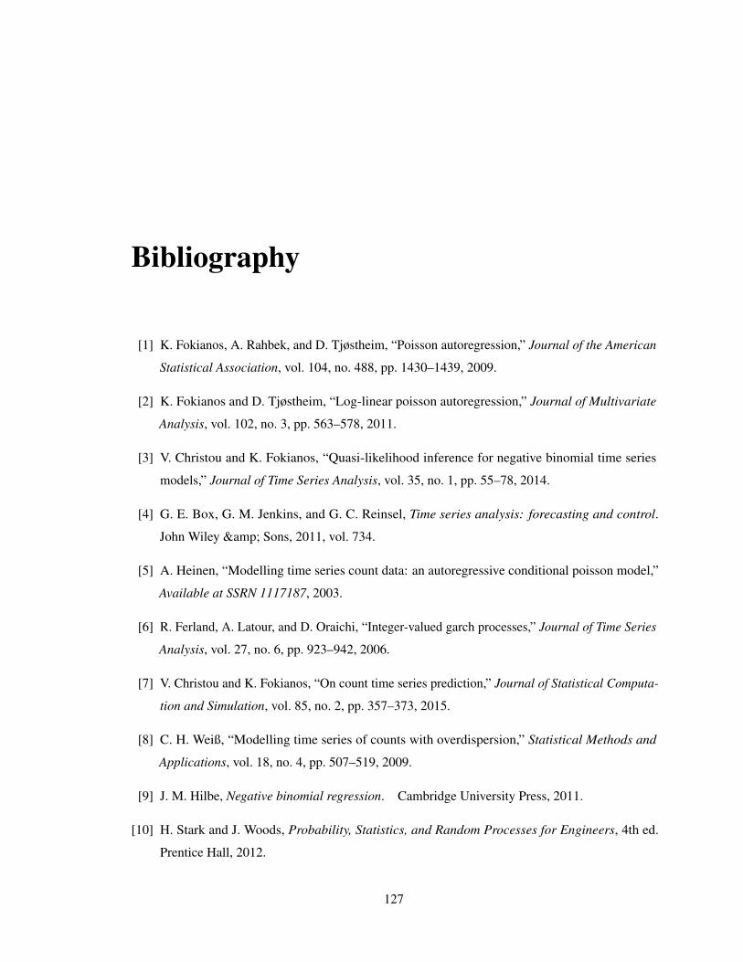
Bibliography
[1] K. Fokianos, A. Rahbek, and D. Tjøstheim, “Poisson autoregression,” Journal of the American
Statistical Association, vol. 104, no. 488, pp. 1430–1439, 2009.
[2] K. Fokianos and D. Tjøstheim, “Log-linear poisson autoregression,” Journal of Multivariate
Analysis, vol. 102, no. 3, pp. 563–578, 2011.
[3] V. Christou and K. Fokianos, “Quasi-likelihood inference for negative binomial time series
models,” Journal of Time Series Analysis, vol. 35, no. 1, pp. 55–78, 2014.
[4] G. E. Box, G. M. Jenkins, and G. C. Reinsel, Time series analysis: forecasting and control.
John Wiley & Sons, 2011, vol. 734.
[5] A. Heinen, “Modelling time series count data: an autoregressive conditional poisson model,”
Available at SSRN 1117187, 2003.
[6] R. Ferland, A. Latour, and D. Oraichi, “Integer-valued garch processes,” Journal of Time Series
Analysis, vol. 27, no. 6, pp. 923–942, 2006.
[7] V. Christou and K. Fokianos, “On count time series prediction,” Journal of Statistical Computa-
tion and Simulation, vol. 85, no. 2, pp. 357–373, 2015.
[8] C. H. Weiß, “Modelling time series of counts with overdispersion,” Statistical Methods and
Applications, vol. 18, no. 4, pp. 507–519, 2009.
[9] J. M. Hilbe, Negative binomial regression. Cambridge University Press, 2011.
[10] H. Stark and J. Woods, Probability, Statistics, and Random Processes for Engineers, 4th ed.
Prentice Hall, 2012.
127

BIBLIOGRAPHY
[11] F. Zhu, “A negative binomial integer-valued garch model,” Journal of Time Series Analysis,
vol. 32, no. 1, pp. 54–67, 2011.
[12] D. G. Manolakis, V. K. Ingle, and S. M. Kogon, Statistical and adaptive signal processing:
spectral estimation, signal modeling, adaptive filtering, and array processing. Artech House
Norwood, 2005, vol. 46.
[13] K. Fokianos, “Count time series models,” Time Series–Methods and Applications, no. 30, pp.
315–347, 2012.
[14] F. Zhu, “Zero-inflated poisson and negative binomial integer-valued garch models,”Journal of
Statistical Planning and Inference, vol. 142, no. 4, pp. 826–839, 2012.
[15] R. Douc, P. Doukhan, and E. Moulines, “Ergodicity of observation-driven time series models and
consistency of the maximum likelihood estimator,” Stochastic Processes and their Applications,
vol. 123, no. 7, pp. 2620–2647, 2013.
[16] B. Kedem and K. Fokianos, Regression models for time series analysis. John Wiley &
Sons, 2005, vol. 488.
[17] R. H. Shumway and D. S. Stoffer, Time series analysis and its applications: with R examples .
Springer Science & Business Media, 2010.
[18] T. Gneiting, F. Balabdaoui, and A. E. Raftery, “Probabilistic forecasts, calibration and sharpness,”
Journal of the Royal Statistical Society: Series B (Statistical Methodology) , vol. 69, no. 2, pp.
243–268, 2007.
[19] A. Brockwell, “Universal residuals: A multivariate transformation,” Statistics & probabil-
ity letters, vol. 77, no. 14, pp. 1473–1478, 2007.
[20] C. Czado, T. Gneiting, and L. Held, “Predictive model assessment for count data,” Biometrics,
vol. 65, no. 4, pp. 1254–1261, 2009.
[21] (2016). [Online]. Available: http://www.ga.gov.au/oracle/nuclear-explosion-query.jsp
128
Appendix A
Model Correlation
A.1 The Linear (1,0) Model
For any linear INGARCH (1,0) model the mean at time n conditioned on In−1 is
λn = d+ axn−1 (A.1)
Assuming stationarity the variance of λn can be expressed as
VΛ = VAR [d+ axn−1] = a2VX (A.2)
Using the variance decomposition and solving for VX yields
VX =VE
1− a2(A.3)
VΛ =a2VE1− a2
(A.4)
To find the dynamics of the (1,0) (A.1) is re-written as:
xn = d+ axn−1 + en0 (A.5)
129

APPENDIX A. MODEL CORRELATION
Continual back substitution of the previous k − 1 values of xn into (A.5) yields
xn = akxn−k +k−1∑i=0
(d+ en−i) ai
= akxn−k + d1− ak
1− a+
k−1∑i=0
aien−i
= akxn−k + µX
(1− ak
)+
k−1∑i=0
aien−i (A.6)
Multiplication of (A.6) by xn−k and taking expectations yields
Rx(k) = akRx(0) + µ2X
(1− a2
)= ak
(VX + µ2
X
)+ µ2
X
(1− a2
)= akVX + µ2
X (A.7)
Since xn is first order stationary the auto-covariance becomes
Cx(k) = akVX (A.8)
Finally, dividing by VX yields the ACF of the linear (1,0) model
ρx(k) = ak (A.9)
To find the correlation of λn re-write (A.1) as
λn = d+ a (λn−1 + en−1) (A.10)
Again continual back substitution of the previous k − 1 values of λn into (A.10) produces
λn = d+
k∑i=1
ai (d+ en−i) + akλn−k
= d1− ak
1− a+
k∑i=1
ai (en−i) + akλn−k
= µΛ
(1− ak
)+
k∑i=1
ai (en−i) + akλn−k (A.11)
Multiplication of (A.11) by λn−k and taking expectations yields
Rλ(k) = akRλ(0) + µ2Λ
(1− ak
)Rλ(k) = ak
(VΛ + µ2
Λ
)+ µ2
Λ
(1− ak
)= akVΛ + µ2
Λ (A.12)
130

APPENDIX A. MODEL CORRELATION
First order stationarity allows the auto-covariance to be expressed as
Cλ(k) = akVΛ (A.13)
and
ρλ(k) = ak (A.14)
To find the cross-correlation between xn and λn multiply (A.1) by xn−k and take expectations to
find for k ≥ 1:
Rλx(k) = µXd+ aRx(k − 1)
= µXd+ a(ak−1VX + µ2
X
)(A.15)
Recognizing that d = (1− a)µX (A.15) simplifies to
Rλx(k) = µ2X + akVX (A.16)
Upon subtraction of µXµΛ the cross-covariance becomes
Cλx(k) = akVX k ≥ 1 (A.17)
ρλx(k) = ak−1 k ≥ 1 (A.18)
Next, to find the cross-covariance for k ≤ 0 we start by re-writing (A.1) as
Rλx(−k) = µXd+ aRx(−k − 1) (A.19)
Since the auto-correlation function is Hermitian symmetric (A.19) can be re-written as
Rλx(−k) = µXd+ aRx(k + 1)
= µXd+ a(ak+1VX + µ2
X
)= µ2
X + ak+2VX (A.20)
and we find that
Cλx(−k) = ak+2VX (A.21)
ρλx(−k) = ak+1 (A.22)
131

APPENDIX A. MODEL CORRELATION
A.2 The Linear (1,1) model
The Linear (1,1) model is defined by its mean recursion equation
d+ axn−1 + bλn−1 (A.23)
Assuming stationarity the variance of the mean can be expressed as
VΛ = VAR [d+ axn−1 + bλn−1] = a2VX + b2VΛ + 2abCxλ(0)
Using (3.25) yields
VΛ = a2VX + b2VΛ + 2abVΛ
=a2VX
1− b2 − 2ab(A.24)
Next, inserting (A.24) into (3.22) and solving produces
VX =a2VX
1− b2 − 2ab+ VE
=VE
1− a2VX1−b2−2ab
= VE1− (a+ b)2 + a2
1− (a+ b)2 (A.25)
(A.26)
To find the correlation of the model we take the same approach used in Section A.1. First we re-write
(A.23) as
xn = d+ axn−1 + bλn−1 + en
= d+ (a+ b) xn−1 − ben−1 + en
= d+ (a+ b) (d+ (a+ b) xn−2 − ben−2) + aen−1 + en
=
k−1∑i=0
d (a+ b)i + (a+ b)k xn−k
+ ak−1∑i=1
(a+ b)i−1 en−i − b (a+ b)k−1 en−k + en
= µX
(1− (a+ b)k
)+ (a+ b)k xn−k
+ a
k−1∑i=1
(a+ b)i−1 en−i − b (a+ b)k−1 en−k + en
(A.27)
132

APPENDIX A. MODEL CORRELATION
Multiplying (A.27) by xn−k and taking expectations yields
Rx(k) = µ2X
(1− (a+ b)k
)+ (a+ b)k Rx(0)− b (a+ b)k−1Rxe(0)
= µ2X + (a+ b)k VX − b (a+ b)k−1 VE
= µ2X + VE (a+ b)k
1− (a+ b)2 + a2
1− (a+ b)2 − b (a+ b)k−1 VE
= µ2X +
VE
1− (a+ b)2
((a+ b)k
(1− (a+ b)2 + a2
))− VE
1− (a+ b)2
(b (a+ b)k−1 + b (a+ b)k+1
)= µ2
X +VE (a+ b)k−1
1− (a+ b)2
((a+ b) − (a+ b) (a+ b)2
)+VE (a+ b)k−1
1− (a+ b)2
(a2 (a+ b) − b+ b (a+ b)2
)= µ2
X +VE (a+ b)k−1
1− (a+ b)2
(a− (a2 + ab) (a+ b) + a2 (a+ b)
)= µ2
X +VE (a+ b)k−1
1− (a+ b)2
(a− a2b− ab2
)= µ2
X + VEa (1− b (a+ b)) (a+ b)k−1
1− (a+ b)2 (A.28)
Upon substitution of VX into (A.28) and solving we find
Rx(k) = µ2X + VX
a (1− b (a+ b)) (a+ b)k−1
1− (a+ b)2 + a2k ≥ 1 (A.29)
From this it is readily found that
Cx(k) = VXa (1− b (a+ b)) (a+ b)k−1
1− (a+ b)2 + a2k ≥ 1 (A.30)
ρx(k) =a (1− b (a+ b)) (a+ b)k−1
1− (a+ b)2 + a2k ≥ 1 (A.31)
133

APPENDIX A. MODEL CORRELATION
Proceeding similarly for the mean series we begin by re-writing (A.23) as
λn = d+ (a+ b) λn−1 + aen−1
= d+ (a+ b) (d+ (a+ b) λn−2 + aen−2) + aen−1
=
k−1∑i=0
d (a+ b)i + (a+ b)k λn−k + a
k∑i=1
(a+ b)i−1 en−i
= µΛ
(1− (a+ b)k
)+ (a+ b)k λn−k + a
k∑i=1
(a+ b)i−1 en−i (A.32)
Multiplying (A.32) by λn−k and taking expectations yields
Rλ(k) = µ2Λ
(1− (a+ b)k
)+ (a+ b)k Rλ(0)
= µ2Λ + (a+ b)k VΛ (A.33)
Thus
Cλ(k) = (a+ b)k VΛ (A.34)
ρλ(k) = (a+ b)k (A.35)
Next, to find the cross-covariance between xn and λn we multiply λn expressed as an infinite
sum by xn−k and take the expectation
Rλx(k) = µΛµX
(1− (a+ b)k
)+ (a+ b)k Rλx(0) + a (a+ b)k−1Rex(0) (A.36)
This result comes from the fact that xn is uncorrelated with any errors that happen later in time.
Continuing to simplify we find
Rλx(k) = µ2Λ
(1− (a+ b)k
)+ (a+ b)k Rλ(0) + a (a+ b)k−1 VE
= µ2Λ + (a+ b)k VΛ + a (a+ b)k−1 VE
= µ2Λ + VE
a2 (a+ b)k
1− (a+ b)2 + a (a+ b)k−1 VE
= µ2Λ + VE
a (a+ b)k−1
1− (a+ b)2
(a (a+ b) + 1− (a+ b)2
)= µ2
Λ + VE(a+ b)k−1 a (1− b (a+ b))
1− (a+ b)2
= µ2X + VX
(a+ b)k−1 a (1− b (a+ b))
1− (a+ b)2 + a2(A.37)
134

APPENDIX A. MODEL CORRELATION
Using (A.37) we additionally find that
Cλx(k) = VX(a+ b)k−1 a (1− b (a+ b))
1− (a+ b)2 + a2(A.38)
Dividing (A.38) by√VXVΛ we find
ρλx(k) = VX(a+ b)k−1 a (1− b (a+ b))
1− (a+ b)2 + a2
√1− b2 − 2ab
a2V 2X
(A.39)
ρλx(k) =(a+ b)k−1 (1− b (a+ b))√
1− b2 − 2abk ≥ 1 (A.40)
To find the cross-covariance when k ≤ 0 we begin by first finding the cross-correlation between
xn and en by multiplying xn as an infinite summation by en−k and taking expectations
Rxe(k) = (a+ b)k Rxe(0)− b (a+ b)k−1 VE (A.41)
=(
(a+ b)k − b (a+ b)k−1)VE (A.42)
= a (a+ b)k−1 VE (A.43)
Next, re-write (A.23) as
λn = d+ (a+ b) xn−1 − ben−1 (A.44)
Multiplication of (A.44) by xn+k and taking the expectation produces
Rλx(k) = µXd+ (a+ b)Rx(k + 1)− bRxe(k + 1) (A.45)
= µXd+ (a+ b)
(µ2X + VE
a (1− b (a+ b)) (a+ b)k
1− (a+ b)2
)− ab (a+ b)k VE
= µ2X +
VE (a+ b)k
1− (a+ b)2
(a (a+ b) − ab (a+ b)2 − ab+ ab (a+ b)2
)= µ2
X + VEa2 (a+ b)k
1− (a+ b)2
= µ2X + VX
a2 (a+ b)k
1− (a+ b)2 + a2k ≤ 0 (A.46)
Thus
Cλx(k) = VXa2 (a+ b)k
1− (a+ b)2 + a2k ≤ 0 (A.47)
ρλx(k) = VXa2 (a+ b)k
1− (a+ b)2 + a2
1√VXVΛ
=a (a+ b)k√1− b2 − 2ab
k ≤ 0 (A.48)
135

APPENDIX A. MODEL CORRELATION
A.3 Linear Zero-Inflated (1,0) Model
To start analyzing the linear zero-inflated (1,0) model (3.9) becomes
λn = d+ axn−1 (A.49)
Despite zero-inflation again
VΛ = a2VX (A.50)
Substituting this result into (3.59) and solving for VX yields
VX =VE
1− a2(1− 2p0)(A.51)
Let Zt and Zf be defined as in Section 3.5 then, using the laws of total probability and iterated
expectations produces
Rex(k) = E [E [enxn−k|Zt]] + E [E [enxn−k|Zf ]] (A.52)
Since Z does not provide any information about xn−k (A.52) becomes
Rex(k) = E [−λnxn−k]
= −Rλx(k) (A.53)
Next, we multiply (A.49) by xn−k and take expectations to find
Rλx(k) = dµX +Rx(k − 1) (A.54)
136

APPENDIX A. MODEL CORRELATION
We then multiply xn = en + λn by xn−k and take expectations to find
Rx(k) = Rex(k) +Rλx(k)
= (1− p0) (dµX + aRx(k − 1))
= (1− p0) (dµX + a (1− p0) (dµX + aRx(k − 2)))
= (1− p0) dµX
k−1∑i=0
(a (1− p0))i + (a (1− p0))k Rx(0)
= dµX (1− p0)1− (a (1− p0))k
1− (a (1− p0))+ (a (1− p0))k
(VX + µ2
X
)(A.55)
= µ2X
(1− (a (1− p0))k
)+ (a (1− p0))k
(VX + µ2
X
)= µ2
X + (a (1− p0))k VX (A.56)
From which we find that
Cx(k) = (a (1− p0))k VX (A.57)
ρx(k) = (a (1− p0))k (A.58)
Next, to find the correlation of λn we multiply λn and λn−k, take expectations, and use (A.49)
to write this as
Rλ(k) = E [(d+ axn−1) (d+ axn−1−k)]
= d2 + 2daµX + a2Rx(k)
= d2 + 2daµX + a2(µ2X + (a (1− p0))k VX
)= µ2
Λ (1− (a (1− p0)))2 + 2a (1− (a (1− p0))) (1− p0)µ2Λ
+ a2 (1− p0)2 µ2Λ + (a (1− p0))k VΛ
= µ2Λ
(1− 2 (a (1− p0)) + (a (1− p0))2 + 2 (a (1− p0)) − 2 (a (1− p0))2
)+ µ2
Λ (a (1− p0))2 + (a (1− p0))k VΛ
Rλ(k) = µ2Λ + (a (1− p0))k VΛ (A.59)
From which we find
Cλ(k) = (a (1− p0))k VΛ (A.60)
ρλ(k) = (a (1− p0))k (A.61)
137
APPENDIX A. MODEL CORRELATION
Finally, to find the cross-covariance between xn and λn we multiply (A.49) by xn−k and take
expectations to find
Rλx(k) = dµX + aRx(k − 1)
=µX (1− a (1− p0))
(1− p0)+ a
(µ2X + (a (1− p0))k−1 VX
)= µXµΛ + ak (1− p0)k−1 VX k ≥ 1 (A.62)
From which
Cλx(k) = ak (1− p0)k−1 VX k ≥ 1 (A.63)
ρλx(k) = (a (1− p0))k−1 k ≥ 1 (A.64)
Next, we multiply (A.49) by xn+k and take expectations to find
Rλx(k) = dµX + aRx(k + 1) (A.65)
from which we find
Rλx(k) = µXµΛ + ak+1 (1− p0)k VX (A.66)
Cλx(k) = ak+1 (1− p0)k VX (A.67)
ρλx(k) = (a (1− p0))k (A.68)
138

Appendix B
Model Estimation
In this appendix we let
L (θ) , L (θ)
represent the likelihood function and log-likelihood function of an observed time series conditioned
on In−1. We have omitted explicit conditioning for the sake of notational simplicity.θ is the vector
of model parameters given below.
θ = {d, a1, . . . , ap, b1, . . . , bp}
We additionally omit the explicit dependence of λn on the model parameters therefore
λn = λn (θ)
B.1 Poisson
Given an observed time series the likelihood of the Poisson model is given by (B.1) and the
log-likelihood function is given by (B.2). Taking the first and second derivatives of (B.2) with
respect to θ yields the observed score vector and observed information, given by (B.3) and (B.4),
139

APPENDIX B. MODEL ESTIMATION
respectively.
L (θ) =N∏n=0
e−λnλxnnxn!
(B.1)
L (θ) =N∑n=0
−λn + xn lnλn − ln Γ (xn + 1) (B.2)
∂L (θ)
∂θ=
N∑n=0
−∂λn∂θ
+xnλn
∂λn∂θ
(B.3)
∂2L (θ)
∂θ∂θT=
N∑n=0
−xnλ2n
∂λn∂θ
(∂λn∂θ
)′+
(1 +
xnλn
)∂2λn∂θ∂θT
(B.4)
B.2 Negative Binomial
Given an observed time series the likelihood of the NB2 model is given by (B.5) and the
log-likelihood function is given by (B.6). The first derivative of (B.6) with respect to ν is given by
(B.7) and the score of (B.6) with respect to θ is given by (B.8).
L (θ, ν) =N∏n=0
Γ (xn + ν)
Γ (ν) Γ (xn + 1)
(ν
λn + ν
)ν ( λnλn + ν
)xn(B.5)
L (θ, ν) =
N∑n=0
ln Γ (xn + ν)− ln Γ (xn + 1)− ln Γ (ν)
+ ν [ln ν − ln (λn + ν)] + xn [lnλn − ln (λn + ν)]
(B.6)
∂L (θ, ν)
∂ν=
N∑n=0
Ψ (λn + ν)−Ψ (ν) + ln ν − ln(λn + ν) + 1− (ν + xn)
λn + ν(B.7)
∂L (θ, ν)
∂θ=
N∑n=0
(− ν
λn + ν+xnλn− xnλn + ν
)∂λn∂θ
=
N∑n=0
(− ν
λn + ν+
xnν
λn(λn + ν)
)∂λn∂θ
=N∑n=0
ν(xn − λn)
λn(λn + ν)
∂λn∂θ
(B.8)
140

APPENDIX B. MODEL ESTIMATION
Taking derivatives of (B.7) and (B.8) give the components of the observed information matrix, given
by (B.9), (B.10), and (B.11)
∂2L (θ, ν)
∂ν2=
N∑n=0
Ψ′ (xn + ν)−Ψ′ (ν) +1
ν− 1
λn + ν
+xn
(λn + ν)2 −λn + ν
(λn + ν)2 +ν
(λn + ν)2
=
N∑n=0
Ψ′ (xn + ν)−Ψ′ (ν) +λn
ν(λn + ν)+
xn − λn(λn + ν)2
=
N∑n=0
Ψ′ (xn + ν)−Ψ′ (ν) +xnν + λ2
n
ν (λn + ν)2 (B.9)
∂2L (θ, ν)
∂θ∂θT=
N∑n=0
ν(xn − λn)
λn(λn + ν)
∂2λn∂θ∂θT
+−ν(λn(λn + ν))− ν(xn − λn)(2λn + φ)
λ2n(λn + ν)2
∂λn∂θ
∂λn∂θ
′
=N∑n=0
ν(xn − λn)
λn(λn + ν)
∂2λn∂θ∂θT
− ν(−λ2n + νxn + 2xnλn)
λ2n(λn + ν)2
∂λn∂θ
∂λn∂θ
′(B.10)
∂2L (θ, ν)
∂ν∂θ=
(− 1
λn + ν+
xn
(λn + ν)2 +ν
(λn + ν)2
)∂λn∂θ
=xn − λn
(λn + ν)2
∂λn∂θ
(B.11)
B.3 ZIP
Let Z be the number of zeros in the observed time series and
f(θ, p0) = p0 + (1− p0) e−λn (B.12)
be the likelihood of observeing a zero value. Then the likelihood and log-likelihood functions of the
ZIP model are given by (B.13) and (B.14), respectively.
L (θ, p0) =f(θ, p0)ZN∏
xn 6=0
(1− p0)e−λnλxnnxn!
(B.13)
L (θ, p0) =Z ln (f(θ, p0)) +∑xn 6=0
ln(1− p0)− λn + xn lnλn − xn (B.14)
141

APPENDIX B. MODEL ESTIMATION
Differentiating (B.12) with respect to p0 and θ yields the score vectors of the ZIP model when
xn = 0, given by (B.15) and (B.16), respectively.
∂f(θ, p0)
∂p0= 1− e−λn (B.15)
∂f(θ, p0)
∂θ= − (1− p0) e−λn
∂λn∂θ
(B.16)
Differentiating (B.15) and (B.16) again yields the observed information components, given by (B.17),
(B.18), and (B.19) respectively, when xn = 0.
∂2f(θ, p0)
∂p20
= 0 (B.17)
∂2f(θ, p0)
∂θ∂θT= (1− p0) e−λn
(− ∂2λn∂θ∂θT
+
(∂λn∂θ
)(∂λn∂θ
)′)(B.18)
∂2f(θ, p0)
∂p0∂θ= e−λn
∂λn∂θ
(B.19)
Now differentiating the log-likelihood function with respect to p0 and θ yields the components of the
observed score vector, given in (B.20) and (B.21).
∂L (θ, p0)
∂p0=∑xn=0
∂f(θ, p0)
∂p0
/f(θ, p0)−
∑xn 6=0
1
1− p0
=∑xn=0
1− e−λnp0 + (1− p0) e−λn
−∑xn 6=0
1
(1− p0)(B.20)
∂L (θ, p0)
∂θ=∑xn=0
∂f(θ, p0)
∂θ
/f(θ, p0)−
∑xn 6=0
∂L (θ, p0xn 6= 0)
∂θ
=
∑xn=0
− (1− p0) e−λn
p0 + (1− p0) e−λn+∑xn 6=0
xnλn− 1
∂λn∂θ
(B.21)
142
APPENDIX B. MODEL ESTIMATION
Further differentiation of (B.20) and (B.21) yields the observed information components of the ZIP
model, given by (B.22), (B.23), and (B.24).
∂2L (θ, p0)
∂p20
=∑xn=0
(∂2f(θ, p0)
∂p20
f(θ, p0)−
(∂f(θ, p0)
∂p0
2))/
f(θ, p0)2
−∑xn 6=0
1
(1− p0)2
=∑xn=0
−(1− e−λn
)2(p0 + (1− p0) e−λn)
2 −∑xn 6=0
1
(1− p0)2 (B.22)
∂2L (θ, p0)
∂θ∂θT=∑xn=0
(∂2f(θ, p0)
∂θ∂θT
)/f(θ, p0)
−(∂f(θ, p0)
∂θ
)(∂f(θ, p0)
∂θ
)T/f(θ, p0)2
=
∑xn=0
− (1− p0) e−λn
p0 + (1− p0) e−λn+∑xn 6=0
xnλn− 1
∂2λn∂θ∂θT
+
∑xn=0
p0 (1− p0) e−λn
(p0 + (1− p0) e−λn)2 −
∑xn 6=0
xnλ2n
(∂λn∂θ
)(∂λn∂θ
)T(B.23)
∂2L (θ, p0)
∂p0∂θ=
(∂2f(θ, p0)
∂p0∂θf(θ, p0)− ∂f(θ, p0)
∂p0
∂f(θ, p0)
∂θ
)/f(θ, p0)2
=e−λn
(p0 + (1− p0) e−λn
)+(1− e−λn
) ((1− p0) e−λn
)(p0 + (1− p0) e−λn)
2
∂λn∂θ
=p0e−λn + (1− p0) e−2λn + e−λn − p0e
−λn − (1− p0) e−2λn
(p0 + (1− p0) e−λn)2
∂λn∂θ
=e−λn
(p0 + (1− p0) e−λn)2
∂λn∂θ
(B.24)
Next we derive the expected value of the score and observed information. Additionally we show
that the expected value of the negative of the observed information matrix is equal to the cumulative
conditional information matrix. All expectations are taken conditioned on In−1, which is omitted for
the sake of brevity. Additionally, the summations are omitted for brevity. Without proof, the first two
moments of the Zero-Truncated Poisson are
E [X] =λeλ
eλ − 1(B.25)
VAR [X] =λeλ
eλ − 1
[1− λ
eλ − 1
](B.26)
143

APPENDIX B. MODEL ESTIMATION
For the ZIP distribution
P [X = 0] = p0 + (1− p0) e−λn (B.27)
P [X 6= 0] = 1− p0 − (1− p0) e−λ = (1− p0)(
1− e−λn)
(B.28)
Using the law of total expectation(B.20) becomes
E[∂L (θ, p0)
∂p0
]=P [X = 0]
1− e−λnp0 + (1− p0) e−λn
− P [X 6= 0]1
(1− p0)(B.29)
Substituting (B.25) through (B.28) into (B.29) yields
=p0 + (1− p0) e−λn1− e−λn
p0 + (1− p0) e−λn
− (1− p0)(
1− e−λn) 1
(1− p0)
=1− e−λn −(
1− e−λn)
=0 (B.30)
Following a similar approach the expected value of (B.21) is re-written as
E[∂L (θ, p0)
∂θ
]=
(P [X = 0]
− (1− p0) e−λn
p0 + (1− p0) e−λn
)∂λn∂θ
+
(P [X 6= 0]
(E [xn|xn > 0]
λn− 1
))∂λn∂θ
(B.31)
Substituting (B.25) through (B.28) into (B.31) yields
= (1− p0)
(−e−λn +
(1− e−λn
)( λne−λn
λn (e−λn − 1)− 1
))∂λn∂θ
=
(− (1− p0) e−λn +
(1− p0)(1− e−λn
)(e−λn − 1)
)∂λn∂θ
=
(− (1− p0) e−λn + (1− p0) e−λn
∂λn∂θ
)=0 (B.32)
We can re-write the expected value (B.22) as
E[∂2L (θ, p0)
∂p20
]= −P [X = 0]
(1− e−λn
)2(p0 + (1− p0) e−λn)
2 − P [X 6= 0]1
(1− p0)2 (B.33)
144

APPENDIX B. MODEL ESTIMATION
Substituting (B.25) through (B.28) into (B.33) yields
=
(1− e−λn
)2(p0 + (1− p0) e−λn)
−(1− e−λn
)(1− p0)
=−(1− e−λn
)(p0 + (1− p0) e−λn) (1− p0)
(B.34)
Similarly (B.23) becomes
E[∂2L (θ, p0)
∂θ∂θT
]=
(P [X = 0]
− (1− p0) e−λn
p0 + (1− p0) e−λn+ P [X 6= 0]
xnλn− 1
)∂2λn∂θ∂θT
+
(P [X = 0]
p0 (1− p0) e−λn
(p0 + (1− p0) e−λn)2 − P [X 6= 0]
xnλ2n
)(∂λn∂θ
)(∂λn∂θ
)T
(B.35)
The first term of (B.35) is equivalent to (B.20) and therefore equals 0
E[∂2L (θ, p0)
∂θ∂θT
]=
(p0 (1− p0) e−λn
p0 + (1− p0) e−λn
)(∂λn∂θ
)(∂λn∂θ
)T
(− (1− p0)
(1− e−λn
) λne−λn
e−λn − 1
)(∂λn∂θ
)(∂λn∂θ
)T
=
(p0 (1− p0) e−λn
p0 + (1− p0) e−λn− (1− p0)
λn
)(∂λn∂θ
)(∂λn∂θ
)T
(B.36)
Last, we find that (B.24) becomes
E[∂2L (θ, p0)
∂p0∂θ
]= P [X = 0]
e−λn
(p0 + (1− p0) e−λn)2
∂λn∂θ
=e−λn
(p0 + (1− p0) e−λn)
∂λn∂θ
(B.37)
To show equivalence of the observed and conditional information matrices we begin by finding
the variance of (B.20)
VAR[∂L (θ, p0)
∂p0
]= P [X = 0]
(1− e−λn
)2(p0 + (1− p0) e−λn)
2 + P [X 6= 0]1
(1− p0)2 (B.38)
which is recognized as−E[∂2L(θ,p0)
∂p20
]. Next, we use the law of total variance to find VAR
[∂L(θ,p0)
∂θ
].
To begin
E[
VAR[∂L (θ, p0)
∂θ
]]= (1− p0)
(1− e−λn
) λne−λnλ2n
(e−λn − 1
)[1− λn
e−λn − 1
]=
(1− p0)
λn
[1− λn
e−λn − 1
](B.39)
145
APPENDIX B. MODEL ESTIMATION
Next,
VAR[E[∂L (θ, p0)
∂θ
]]=
(P [X = 0]
((1− p0) e−λn
)2(p0 + (1− p0) e−λn)
2
)(∂λn∂θ
)(∂λn∂θ
)T
+
(P [X 6= 0]
1
(e−λn − 1)2
)(∂λn∂θ
)(∂λn∂θ
)T
=
( ((1− p0) e−λn
)2(p0 + (1− p0) e−λn)
+(1− p0) e−λn
(e−λn − 1)
)(∂λn∂θ
)(∂λn∂θ
)T
=
((1− p0)2 e−λn − (1− p0)2 e−2λn
(p0 + (1− p0) e−λn) (e−λn − 1)
)(∂λn∂θ
)(∂λn∂θ
)T
+
(p0 (1− p0) e−λn + (1− p0)2 e−2λn
(p0 + (1− p0) e−λn) (e−λn − 1)
)(∂λn∂θ
)(∂λn∂θ
)T
=
((1− p0)2 e−λn + p0 (1− p0) e−λn
(p0 + (1− p0) e−λn) (e−λn − 1)
)(∂λn∂θ
)(∂λn∂θ
)T
=
((1− p0) e−λn
(p0 + (1− p0) e−λn) (e−λn − 1)
)(∂λn∂θ
)(∂λn∂θ
)T
(B.40)
Combining (B.39) and (B.40) produces
VAR[∂L (θ, p0)
∂θ
]=
((1− p0)
λn− p0
e−λn − 1
)(∂λn∂θ
)(∂λn∂θ
)T
+
((1− p0) e−λn
(p0 + (1− p0) e−λn) (e−λn − 1)
)(∂λn∂θ
)(∂λn∂θ
)T
=
((1− p0)
λn+
(1− p0)[e−λn − p0 − e−λn + p0e
−λn]
(p0 + (1− p0) e−λn) (e−λn − 1)
)(∂λn∂θ
)(∂λn∂θ
)T
=
((1− p0)
λn−
p0 (1− p0)(1− e−λn
)(p0 + (1− p0) e−λn) (e−λn − 1)
)(∂λn∂θ
)(∂λn∂θ
)T
=
((1− p0)
λn− p0 (1− p0) e−λn
p0 + (1− p0) e−λn
)(∂λn∂θ
)(∂λn∂θ
)T
(B.41)
Finally we find the covariance of (B.20) and (B.21), given by (B.42) where we have taken advantage
of the fact that both are 0 mean.
COV[∂L (θ, p0)
∂p0,∂L (θ, p0)
∂θ
]= E
[∂L (θ, p0)
∂p0
∂L (θ, p0)
∂θ
](B.42)
146

APPENDIX B. MODEL ESTIMATION
Inserting (B.20) and (B.21) into (B.42) produces
= −
(e−λn (1− p0)
(1− e−λn
)p0 + (1− p0) e−λn
+(1− p0)
(1− e−λn
)(1− p0) (e−λn − 1)
)∂λn∂θ
= −
(e−λn (1− p0)
(1− e−λn
)p0 + (1− p0) e−λn
+ e−λn
)∂λn∂θ
= −
(e−λnp0 + (1− p0) e−2e−λn + (1− p0) e−λn − (1− p0) e−2e−λn
p0 + (1− p0) e−λn
)∂λn∂θ
= − e−λn
p0 + (1− p0) e−λn∂λn∂θ
(B.43)
Equations (B.39) through (B.43) are equal to the negative expected value of the observed information
matrix, as expected.
B.4 ZINB2
To find the score and observed information of the ZINB2 model we let
y = f(x)x (B.44)
ln y = x ln f(x) (B.45)
implicit differention of (B.45) yields
y′
y= ln f(x) + x
f ′(x)
f(x)
y′ = y
[ln f(x) + x
f ′(x)
f(x)
](B.46)
Implicitly differentiating (B.46) again we find
y′′ = y′[ln f(x) + x
f ′(x)
f(x)
]+ y
[f ′(x)
f(x)+f ′(x)
f(x)+ x
(f ′′(x)f(x)− (f ′(x))2
f(x)2
)]
y′′ = y′[ln f(x) + x
f ′(x)
f(x)
]+ y
[2f ′(x)
f(x)+ x
f ′′(x)
f(x)− x
(f ′(x)
f(x)
)2]
y′′ = y
[ln f(x) + x
f ′(x)
f(x)
]2
+ y
[2f ′(x)
f(x)+ x
f ′′(x)
f(x)− x
(f ′(x)
f(x)
)2]
(B.47)
147

APPENDIX B. MODEL ESTIMATION
Next we let f(ν,θ) = νλn+ν and differentiate to find the score, given by (B.48) and (B.49).
∂f(ν,θ)
∂ν=λ+ ν − ν(λn + ν)2 =
λn
(λn + ν)2 (B.48)
∂f(ν,θ)
∂θ= − ν
(λn + ν)2
∂λn∂θ
(B.49)
Further differentiation produces the information matrix of f(ν,θ), given by (B.50), (B.51), and
,(B.52).
∂2f(ν,θ)
∂ν2= − 2λn
(λn + ν)3 (B.50)
∂2f(ν,θ)
∂θ2=
2ν
(λn + ν)3
(∂λn∂θ
)(∂λn∂θ
)T
− ν
(λn + ν)2
∂2λn∂θ∂θT
(B.51)
∂2f(ν,θ)
∂ν∂θ=
(λn + ν)2 − 2λn(λn + ν)
(λn + ν)4
∂λn∂θ
=λn + ν − 2λn
(λn + ν)3
∂λn∂θ
=ν − λn
(λn + ν)3
∂λn∂θ
(B.52)
Next we let
g(ν,θ) = f(ν,θ)ν =
(ν
λn + ν
)ν(B.53)
From (B.53) we observe that g(ν,θ) is in the form of (B.44) when differentiated with respect to ν.
Using (B.46) yields (B.54).
∂g(ν,θ)
∂ν= g(ν,θ)
(ln f(ν,θ) + ν
∂f(ν,θ)∂ν
f(ν,θ)
)
=
(ν
λn + ν
)νlnν
λn + ν+ ν
λn(λn+ν)2
νλn+ν
=
(ν
λn + ν
)ν (ln
ν
λn + ν+
λnλn + ν
)(B.54)
Next, we take the derivative of (B.53) with respect to θ to yield (B.55) and (B.56)
.∂g(ν,θ)
∂θ= νf(ν,θ)ν−1∂f(ν,θ)
∂θ= − ν
(λn + ν)2 ν
(ν
λn + ν
)ν−1 ∂λn∂θ
= − νν+1
(λ+ ν)ν+1
∂λn∂θ
(B.55)
= −g(ν,θ)f(ν,θ)∂λn∂θ
(B.56)
148

APPENDIX B. MODEL ESTIMATION
Taking the derivative of (B.54) with respect to ν we find
∂2g(ν,θ)
∂ν2=g(ν,θ)
(ln f(ν,θ) + ν
∂f(ν,θ)∂ν
f(ν,θ)
)2
+ g(ν,θ)
2∂f(ν,θ)∂ν
f(ν,θ)+ ν
∂2f(ν,θ)∂ν2
f(ν,θ)− ν
(∂f(ν,θ)∂ν
f(ν,θ)
)2
=
(ν
λn + ν
)νlnν
λn + ν+ ν
λn(λn+ν)2
νλn+ν
2
+
(ν
λn + ν
)ν2
λn(λn+ν)2
νλn+ν
+ ν− 2λn
(λn+ν)3
νλn+ν
− ν
λn(λn+ν)2
νλn+ν
2=
(ν
λn + ν
)ν (ln
ν
λn + ν+ ν
λnνλn + ν
)2
+
(ν
λn + ν
)ν (2λn(λn + ν)
ν (λn + ν)2 −2λnν
ν (λn + ν)2 −λ2n
νλn + ν
)=
(ν
λn + ν
)ν (ln2 ν
λn + ν+
2λnλn + ν
lnν
λn + ν+
λ2nν + λ2
n
ν (λn + ν)2
)(B.57)
Last, taking the derivative of (B.56) yields
∂2g(ν,θ)
∂θ2=
(−∂g(ν,θ)
∂θf(ν,θ)− ∂f(ν,θ)
∂θg(ν,θ)
)∂λn∂θ
+∂g(ν,θ)
∂θ
∂2λn∂θ∂θT
(B.58)
=−(
ν
λn + ν
)ν+1(
ν
λn + ν− ν
(λn + ν)2
(ν
λn + ν
)−1)(
∂λn∂θ
)(∂λn∂θ
)T
−(
ν
λn + ν
)ν+1 ∂2λn∂θ∂θT
=
(ν
λn + ν
)ν (( ν
λn + ν
)2
− ν
(λn + ν)2
)(∂λn∂θ
)(∂λn∂θ
)T
−(
ν
λn + ν
)ν+1 ∂2λn∂θ∂θT
(B.59)
and
∂2g(ν,θ)
∂ν∂θ=
(∂g(ν,θ)
∂νf(ν,θ)− ∂f(ν,θ)
∂νg(ν,θ)
)∂λn∂θ
(B.60)
= −(
ν
λn + ν
)ν (ln
ν
λn + ν+
λnλn + ν
)ν
λn + ν−(
ν
λn + ν
)ν λn
(λn + ν)2
∂λn∂θ
= −(
ν
λn + ν
)ν ( ν
λn + νln
ν
λn + ν+λnν + λn
(λn + ν)2
)∂λn∂θ
(B.61)
149

APPENDIX B. MODEL ESTIMATION
Next we let and using the results for g(ν,θ) find
h(p0, ν,θ) = p0 + (1− p0)
(ν
λn + ν
)ν= p0 + (1− p0)g(ν,θ) (B.62)
h(p0, ν,θ) = p0 + (1− p0)
(ν
λn + ν
)ν(B.63)
∂h(p0, ν,θ)
∂p0= 1−
(ν
λn + ν
)ν(B.64)
∂h(p0, ν,θ)
∂ν= (1− p0)
(ν
λn + ν
)ν (ln
ν
λn + ν+
λnλn + ν
)(B.65)
∂h(p0, ν,θ)
∂θ= − (1− p0)
(ν
λn + ν
)ν+1
(B.66)
∂2h(p0, ν,θ)
∂p20
= 0 (B.67)
∂2h(p0, ν,θ)
∂ν2= (1− p0)
(ν
λn + ν
)ν (ln2 ν
λn + ν+
2λnλn + ν
lnν
λn + ν+
λ2nν + λ2
n
ν (λn + ν)2
)(B.68)
∂2h(p0, ν,θ)
∂θ∂θT= (1− p0)
(ν
λn + ν
)ν+2
+ν
(λn + ν)2
(ν
λn + ν
)ν(B.69)
∂2h(p0, ν,θ)
∂p0∂ν= −
(ν
λn + ν
)ν (ln
ν
λn + ν+
λnλn + ν
)(B.70)
∂2h(p0, ν,θ)
∂p0∂θ=
(ν
λn + ν
)ν+1
(B.71)
∂2h(p0, ν,θ)
∂ν∂θ= (1− p0)−
(ν
λn + ν
)ν ( ν
λn + νln
ν
λn + ν+λnν + λn
(λn + ν)2
)(B.72)
150

APPENDIX B. MODEL ESTIMATION
Finally we let Z be the number of zeros in xn then and find
L (θ, ν, p0) = h(p0, ν,θ)Z +N∏
xn 6=0
L (ν,θ|xnxn 6= 0) (B.73)
L (θ, ν, p0) = Z ln(h(p0, ν,θ)) +∑xn 6=0
ln(1− p0) + L (ν,θ|xnxn 6= 0)NB (B.74)
∂L (θ, ν, p0)
∂p0=∂h(p0, ν,θ)
∂p0
/h(p0, ν,θ) (B.75)
=1−
(ν
λn+ν
)νp0 + (1− p0)
(ν
λn+ν
)ν (B.76)
∂L (θ, ν, p0)
∂ν=∂h(p0, ν,θ)
∂ν
/h(p0, ν,θ) (B.77)
∂L (θ, ν, p0)
∂θ=∂h(p0, ν,θ)
∂θ
/h(p0, ν,θ) (B.78)
∂2L (θ, ν, p0)
∂p20
=
(∂2h(p0, ν,θ)
∂p20
−(∂h(p0, ν,θ)
∂p0
)2)/
h(p0, ν,θ)2 (B.79)
∂2L (θ, ν, p0)
∂ν2=
(∂2h(p0, ν,θ)
∂ν2−(∂h(p0, ν,θ)
∂ν
)2)/
h(p0, ν,θ)2 (B.80)
∂2L (θ, ν, p0)
∂θ∂θT=
(∂2h(p0, ν,θ)
∂θ∂θT−(∂h(p0, ν,θ)
∂θ
)(∂h(p0, ν,θ)
∂θ
)′)/h(p0, ν,θ)2 (B.81)
∂2L (θ, ν, p0)
∂p0∂ν=
(∂2h(p0, ν,θ)
∂p0∂ν− ∂h(p0, ν,θ)
∂p0
∂h(p0, ν,θ)
∂ν
)/h(p0, ν,θ)2 (B.82)
∂2L (θ, ν, p0)
∂p0∂θ=
(∂2h(p0, ν,θ)
∂p0∂θ− ∂h(p0, ν,θ)
∂p0
∂h(p0, ν,θ)
∂θ
)/h(p0, ν,θ)2 (B.83)
∂2L (θ, ν, p0)
∂ν∂θ=
(∂2h(p0, ν,θ)
∂ν∂θ− ∂h(p0, ν,θ)
∂ν
∂h(p0, ν,θ)
∂θ
)/h(p0, ν,θ)2 (B.84)
(B.85)
151