GEON LiDAR Workflow (GLW) output and ArcMap Users Guide

Joshua Coyan Christopher Crosby Ramón Arrowsmith

School of Earth and Space Exploration Arizona State University

24 October 2007

http://lidar.asu.edu

Table of Contents Importing GLW output into ArcMap............................................................................. 2 Defining the projection ..................................................................................................... 7 Producing a Hillshade Map............................................................................................ 12 Printing the map ............................................................................................................. 17 Other activities ................................................................................................................ 23

Making a contour map .................................................................................................. 23 Topographic profiles..................................................................................................... 26

1

Importing GLW output into ArcMap

Open ArcMap and click on the toolbox button.

Click on the toolbox button to open the toolbox window.

The toolbox window will open as a pane as shown below.

2

Click on the Conversion Tools option. This will expand the menu.

Click on the To Raster option. This menu will expand further.

3

Select the ASCII to Raster option.

This opens a new window. Specify the file you would like to import, the name and location for the output and finally under Output Data Type (optional) select Float.

Click here and select FLOAT for the Output data type.

Click here to navigate to where you would like to save the output raster.

Click here to navigate to where you have saved *.arc.asc file types.

4

Note: based on your default settings, you may need to specify the file type listed.

Once you have navigated to where you have stored *.arc.asc data you may need to specify the file types shown. Note: on many computers *.txt files are the default displayed file types.

Based on the size of your data set, it may take a moment for the calculation to complete. Once it has completed, the window will give you a notice that says the job has completed click Close.

This window summarizes the calculation of ASCII to Raster. When the status is Complete, click Close.

5

Now on the left windowpane, under the layer you just added, right click on the layer and click Zoom to layer.

Right click on the Layer you just imported and then click Zoom to Layer.

6

Defining the projection You may not need to project the data (change the datum or projection). But, the DEM products delivered from the GLW are not internally defined in terms of their coordinate systems. You can work with them by themselves without this definition, but if you want to combine them with other data, you will need to define it. If you have Arc Map open, you should close it so that there will not be a complaint from the other software, ArcCatalogue about the files being busy. The example we give here is for the B4 LiDAR data which has these coordinate system attributes:

Grid Coordinate System Name: Universal Transverse Mercator UTM Zone Number: 11 N Transverse Mercator Projection Scale Factor at Central Meridian: 0.999600 Longitude of Central Meridian: -117.000000 Latitude of Projection Origin: 0.000000 False Easting: 500000.000000 False Northing: 0.000000 Planar Coordinate Information: Planar Distance Units: meters Geodetic Model Horizontal Datum Name: D_WGS_1984 Ellipsoid Name: WGS_1984

Launch ArcCatalogue: Start->Programs->ArcGIS->ArcCatalogue Then Right click on the Raster file you made in the last step and select properties (see next page)

7

8

Scroll down to the Spatial reference which will be undefined and click on Edit:

9

Choose to Define the coordinate system interactively. Scroll to the bottom of the list of projections and choose UTM:

Units should be meters, zone is 11 (in this case), and X shift is the False Easting of 500,000:

Set the datum (in this case) as WGS84:

10

The final screen should look like this:

11

Producing a Hillshade Map After you have loaded the data and projected it, click on the Spatial Analyst tool. If you do not have the Spatial Analyst tool in your toolbar, select Toolbars from the View menu. Then click Spatial Analyst from the pop up window.

To access the Spatial Analyst tool, click View.

Select the Toolbars option from the View menu.

Click on Spatial Analyst.

Drag the Spatial Analyst toolbar to your toolbar.

12

If this is the first time you have used the Spatial Analyst tool, you may need to turn on the extensions. To turn on the extensions, select the Extensions option from the Tools menu.

Check the 3D Analyst and the Spatial Analyst options, click Close.

13

Now to make a hillshade map, select the Surface Analysis option under the Spatial Analyst pull down menu. Click on Hillshade.

Selects the input surface to be modeled.

The direction the illumination will come from

The angle of the illumination source from the horizon.

This can be interesting to play with

For more information about this window, click ? and then select the option of interest.

Click Ok to create the hillshade.

14

Step 4 Combining the Hillshade and DEM, creating a color map If you have the DEM and hillshade loaded make sure that the DEM is on top in the Layers pane. This can be done by simply clicking on the desired layer and dragging it above the hillshade. To color the DEM, right click on the DEM and select Properties then click on the Symbology tab.

Click on the Symbology tab.

Click on the color ramp pull down window to select the color scheme of your liking.

15

Once you have chosen a color scheme click on the Display tab. Change the Transparency setting to 50%. Then click Ok.

Click on the Display tab. Change the Transparency setting to 50%.

The effects can be astonishing. Now you have a colored map.

16

Printing the map To print the map, first change from the Data View to the Layout View.

Layout View Data View

You will now see how the image will look on an 8.5 x 11 sheet of paper.

17

You can now see how the image will be centered and look on an 8.5 x 11 sheet of paper. You can now stretch the image or shrink the image by using the arrow button and clicking on the image. You can use the hand tool and adjust what part of the image is seen. You can also change the paper properties by choosing the Page and Print Setup option from the File menu.

To add a scale bar, legend, and compass rose click on the Insert menu at the top of your screen.

Select Legend to add a legend to your map.

Select North Arrow to add a compass rose to your map.

Click Scale Bar to add a scale to your map.

18

When you choose Legend, a new window will open like the one below. Remove the hillshade map and click Next.

Once you have highlighted the Hillshade item, click the remove link to remove this item. Click on the

Hillshade item

You can then click through the next four windows keeping the default settings or you can specify the options you would like for your legend. For more information about legend options, see the Arc help pages. The end of this document goes through a tutorial on cleaning up the legend: http://arrowsmith410-598.asu.edu/Lectures/Lecture9/DEM_data.html.

19

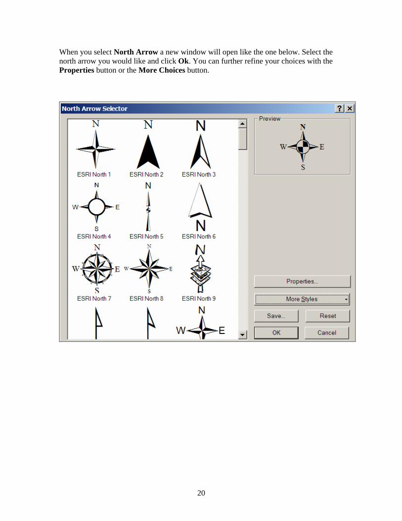
When you select North Arrow a new window will open like the one below. Select the north arrow you would like and click Ok. You can further refine your choices with the Properties button or the More Choices button.

20

When you select Scale Bar a new window will open like the one below. Select the style of scale bar you would like and click Ok. You can further refine your choices and you can define the units with the Properties button or the More Choices button.

21

To print the map, select Print from the File menu. A window will open like the one below. Here you can specify the options you would like. When you are satisfied with your options, click Ok.

22

Other activities Making a contour map Select the Surface Analysis option under the Spatial Analyst pull down menu. Click on Contour. Make sure that the target layer is your Raster DEM, not the Hillshade!

23

This screen will appear:

Make sure this is the correct file (should be the DEM)

Define the contour interval

Save the contours if you want

24

To label the contours, right click on the contours layer and choose Label features:

The problem will be that the labels will probably be for the line ID and not the elevation! So, then right click on the layer again, but this time choose Properties->Label Tab, and make sure that the Label Field is CONTOUR:

25

Topographic profiles To make a topographic profile along a path you define on the DEM, do the following: You will need the 3D analyst tool, so make sure that under extensions, its check box is checked (as you did above for the Spatial Analyst). Then under View->Toolbars->3DAnalyst, select that and the toolbar will appear. Make sure that the target layer is the DEM you have made above, and then click on the little symbol that looks like a squiggle. It is the Interpolate line tool.

Use that tool to define your profile. Click once to start, and then click for each vertex along your profile (it does not have to be a single straight line profile). Double click at the end. When you double click, it may take quite a while (tens of seconds) at first for anything to happen. The program is going through the DEM and finding your pixels that are nearest to the line you chose.

To actually draw the profile, click on the symbol that looks like a profile (Create Profile Graph above).

26

If you right click on the resulting plot, you can set various parameters of the plot (labels, etc.) by choosing the Properties and Advanced Properties.

One choice under that menu (the one above that you get when right clicking on the plot), is Export. This is a new addition it seems in ArcGIS9.2. You can export the data from your profile to something like Microsoft Excel. Choose the Data tab and then the Excel format. This will export a two column XY or Distance-Elevation file that one can use for further analysis.

27