1

Lessons Taught by James Wilkinson

Margaret H. Wright

Computer Science Department

Courant Institute of Mathematical Sciences

New York University

Workshop on “Advances in Numerical Linear Algebra”

School of Mathematics

University of Manchester

Manchester, England

May 29, 2019

Many thanks to Nick Higham, Sven Hammarling, and

Francoise Tisseur for organizing the workshop!

2

The context for this talk. . .

Jim’s primary career was as a member of the British Scientific

Civil Service at the National Physical Laboratory (NPL) in

Teddington, England, which in its heyday was a center for

basic research in a wide range of fields of science and

engineering. (Alan Turing worked at NPL from 1945–1948.)

Jim was appointed at the NPL in 1946, partly in the General

Computing Section and partly in the ACE (Automatic

Computing Engine) section to work with Alan Turing. He

remained at NPL until he retired in 1980. Starting in 1958,

he also taught numerical linear algebra in summer schools at

the University of Michigan. (Cleve Moler joined Jim as a

lecturer in the Michigan courses in 1966.)

3

Jim visited Stanford for short periods during the 1960s,

hosted by Gene Golub, and wrote several technical reports.

Starting in the early 1970s, Jim regularly visited and lectured

at Argonne National Laboratory.

Sometime in the late 1970s, he was officially appointed as a

visiting professor in the Computer Science Department at

Stanford for one term per year. (The dates given for this vary

slightly from source to source.)

Those Stanford courses were the inspiration for this talk,

which draws from material contained in Jim’s lecture notes.

Some of the notes include dates, and from those we know

that he taught ‘CS 237A’, ‘CS 237B’, and ‘CS 238B’ in

1977–1982.

4

The following people (students and/or attendees in Jim’s

courses) graciously made lecture notes as well as homework

problems and solutions available, and also contributed

anecdotes and insights—thank you, all!

Petter Bjørstad John Lewis

William Coughran Stephen Nash

Walter Gander Michael Overton

Eric Grosse Michael Saunders

Michael Heath L. N. Trefethen

Linda Kaufman Raymond Tuminaro

Steven Leon Patrick Worley

Randall LeVeque

5

The available lecture notes address two broad topics:

1. Linear systems and error analysis

2. Eigenvalues

And there are associated homework problems, some involving

computation, and their solutions.

Reading the notes all together makes clear that, although

there is overlap in the topics covered, the results are

presented sometimes in a different order, sometimes from a

different perspective.

As does everyone who teaches, it is evident that Jim

continued to rework the material, altering motivation,

explanations, and examples.

6

A question for today: what to include in this 25-minute talk?

Definitely not eigenvalues, a topic that Jim begins by saying

It is our intention to motivate the whole of the background

theory of the algebraic eigenvalue problem by consideration of

linear differential equations.

For reasons of practicality, this talk will focus on selected parts

of “Supplementary notes for CS237b, Winter Quarter 1982”.

Following background about linear algebra, Jim turns to

computing the solution x of Ax = b. Let ǫ denote a modest

multiple of machine precision.

An aspect that he mentions early on, and repeatedly, is the

“size” of x.

7

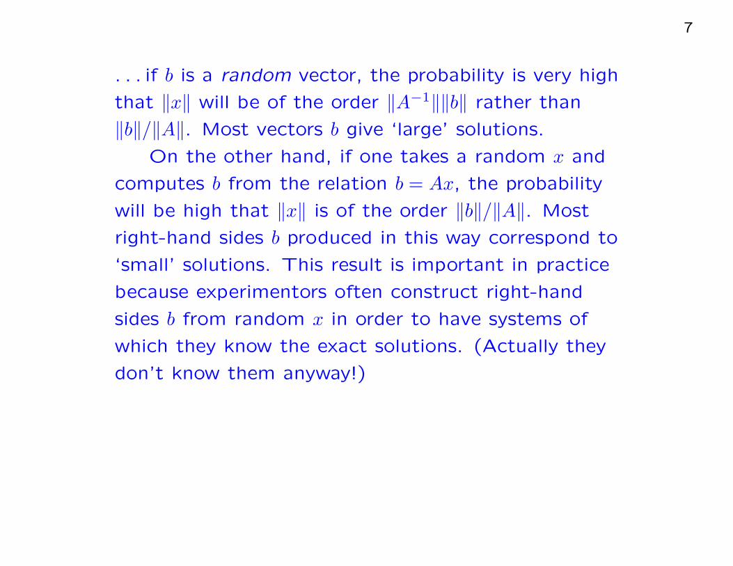
. . . if b is a random vector, the probability is very high

that ‖x‖ will be of the order ‖A−1‖‖b‖ rather than

‖b‖/‖A‖. Most vectors b give ‘large’ solutions.

On the other hand, if one takes a random x and

computes b from the relation b = Ax, the probability

will be high that ‖x‖ is of the order ‖b‖/‖A‖. Most

right-hand sides b produced in this way correspond to

‘small’ solutions. This result is important in practice

because experimentors often construct right-hand

sides b from random x in order to have systems of

which they know the exact solutions. (Actually they

don’t know them anyway!)

8

Jim considers the correctly rounded version of x when x is not

representable, namely x+ w with ‖w‖ ≤ ǫ‖x‖, and shows that

even this paragon of virtue among approximate solutions

cannot be expected to give a smaller residual than the exact

solution y of (A+ δA)y = b with ‖δA‖ ≤ ǫ‖A‖.

In each set of notes, considerable space is devoted to matrix

inversion. Here is a summary of the high points.

The exact inverse X is characterized by four properties, each

of which is associated with a measure of excellence of an

approximate inverse Y .

9

Property Measure

X −A−1 = 0 1. ‖Y −A−1‖/‖A−1‖

X−1 −A = 0 2. ‖Y −1 −A‖/‖A‖

AX − I = 0 3. ‖AY − I‖

XA− I = 0 4. ‖Y A− I‖

Let κ = ‖A‖‖A−1‖, the condition number of A.

Jim reviews these four choices of Y with respect to the given

measures.

The point of interest is that the condition number κ obtrudes

in the upper bounds on the measures for some choices of Y

and some tests.

10

1. Consider Y1 = (A+ δA)−1, with ‖δA‖ ≤ ǫ‖A‖, so that Y1 is

the exact inverse of a near neighbor of A. Then

(test 2)‖Y −1

1 −A‖

‖A‖=

‖δA‖

‖A‖≤ ǫ (good), but

(test 1)‖Y1 −A−1‖

‖A−1‖≤

ǫκ

1− ǫκ. (κ obtrudes).

The factor κ also obtrudes in tests 3 and 4.

2. What about Y2 = A−1 +W , where ‖W‖ ≤ ǫ‖A−1‖, so that

Y2 is a near neighbor of the exact inverse of A? By

definition, Y2 is good for test 1, but κ obtrudes in tests 3

and 4.

11

3. Y3 is defined by

AY3 − I = R, with ‖R‖ ≤ ǫ.

Then

‖Y3 −A−1‖

‖A−1‖≤ ǫ (test 1) and

‖A− Y −13 ‖

‖A‖≤

ǫ

1− ǫ(test 2).

However,

‖Y3A− I‖ ≤ ǫκ. (test 4)

4. Finally, if Y4 is defined by Y4A− I = R with ‖R‖ ≤ ǫ, Y4

does well in tests 1 and 2, but κ obtrudes into the bound

in test 3.

12

What about A−1R

, the correctly rounded version of A−1, which

satisfies

A−1R

= A−1 + E, where ‖E‖ ≤ ǫ‖A−1‖.

How does A−1R

perform on the different tests?

The corresponding relations are

AA−1R

= A(A−1 + E) = I +AE, with ‖AE‖ ≤ ‖A‖‖E‖ ≤ ǫκ

so that κ obtrudes and this bound will usually be realistic.

13

Suppose we want to compute the explicit inverse X.

This is typically done by solving for xi, the i-th column of X,

from

Axi = ei,

where ei is the i-th coordinate vector.

Our expectation is that we will obtain yi (the computed i-th

column of X) that satisfies

(A+ δAi)yi = ei with ‖δAi‖ ≤ ǫ‖A‖.

Note that in general δAi will be different for each i.

Jim asks: how ’good’ would Y be?

Answer: apply the four tests.

14

Note that AY = I −(

δA1 y1 δA2 y2 . . . δAn yn

)

△

= I −E. We

have ‖E‖ ≤ ǫ‖A‖‖Y ‖, so that

‖Y ‖ ≤‖A−1‖

1− ǫκand ‖AY − I‖ ≤

ǫκ

1− ǫκ.

Given these bounds, Y performs just as well on test 3 as the

inverse of A+ δA.

For test 4, however, we have Y A− I = A−1(AY − I)A, so that

‖Y A− I‖ ≤ κ‖AY − I‖ ≤ǫκ2

1− ǫκ,

with an ’extra’ factor of κ.

15

The bound involving κ2 calls for further comments. It is

realistic only when the δAi are random, uncorrelated

perturbations satisfying ‖δiA‖ ≤ ǫ‖A‖.

In practice, when computing the columns of an inverse by a

stable direct method, although the δAi are all different, they

are not a random set. They are related in such a way that we

can expect ‖Y A− I‖ to be of the same order of magnitude as

‖AY − I‖.

The extra factor κ does not materialize.

16

In order to emphasize that the ‘accumulation of errors’ is not

the important feature we consider approximate inverses for an

ill-conditioned 2× 2 example:

A =

0.8623 0.7312

0.8177 0.6935

, with κ ≈ 2.36× 104.

Here are A−1 and an approximate inverse Y :

A−1 =104

1.0281

0.6935 −0.7312

−0.8177 0.8623

Y = 104

0.6745 −0.7112

−0.7954 0.8387

.

17

We have (exactly)

AY =

0.2487 −0.1032

−0.7125 0.9021

and Y A =

0.7311 −0.2280

−0.6843 0.4197

so that ‖AY − I‖ and ‖Y A− I‖ are O(1).

We cannot expect them to be small because A−1 is so large

that the mere act of rounding to 4 decimals introduces errors

of order unity that are almost certain to be uncorrelated.

18

The exact inverse of Y is given by

Y −1 =1

0.1467

0.8387 0.7112

0.7954 0.6745

=

5.7171 . . . 4.8479 . . .

5.4219 . . . 4.5978 . . .

.

Hence Y −1 differs from A by quantities of O(1). This is to be

expected given that κ = O(104). However, Y −1 is wrong in

rather a strange way. To four significant decimals,

Y −1 = 6.630A, i.e. Y −1 is almost a multiple of A.

Can you explain why?

19

Now we consider an approximate inverse Z in which z1 and z2

are the first and second columns of the inverses of

A+δA1 =

0.8624 0.7323

0.8177 0.6935

and A+δA2 =

0.8623 0.7312

0.8177 0.6936

,

where ‖δAi‖ = 10−4 and δ1A 6= δ2A.

The exact z1 and z2 are

z1 =104

1.7216

0.6935

−0.8177

≈ 104

0.4028

−0.4750

z2 =104

1.8904

0.7312

0.8623

≈ 104

−0.3868

0.4561

.

20

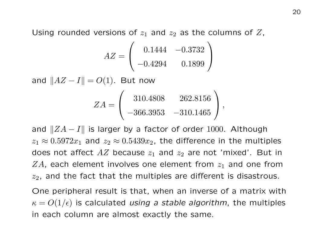
Using rounded versions of z1 and z2 as the columns of Z,

AZ =

0.1444 −0.3732

−0.4294 0.1899

and ‖AZ − I‖ = O(1). But now

ZA =

310.4808 262.8156

−366.3953 −310.1465

,

and ‖ZA− I‖ is larger by a factor of order 1000. Although

z1 ≈ 0.5972x1 and z2 ≈ 0.5439x2, the difference in the multiples

does not affect AZ because z1 and z2 are not ’mixed’. But in

ZA, each element involves one element from z1 and one from

z2, and the fact that the multiples are different is disastrous.

One peripheral result is that, when an inverse of a matrix with

κ = O(1/ǫ) is calculated using a stable algorithm, the multiples

in each column are almost exactly the same.

21

Leaving matrix inverses and moving on to error analysis, Jim

repeats that error analysis has concentrated too much on the

details of floating point, which is unfortunate because the

important features of the results are often really quite

independent of these details. They would remain the same

even if we were considering computation with integers and the

old errors were blunders.

In this spirit, he introduces a formalism in which a quantity to

be computed is defined in terms of known quantities by a very

simple equation. If the new computed quantity is inserted into

the equation, a discrepancy may arise because of computing

errors. But the discrepancy is merely the sum of all errors

made during the computation; there is no interaction.

We do not concern ourselves with what the various quantities

would have been if we had produced them exactly. This

apparently trivial remark is of vital importance.

22

A familiar relation in Gaussian elimination is MA(n) = A+∆,

which can be looked at in two different ways.

We can say that we have computed M and A(n) and in order

to assess our performance we are looking at MA(n) −A. This

is a perfectly natural approach. It pervades the whole of

numerical analysis. the whole of numerical analysis.

Alternatively we could say that if we take A+∆ and do

Gaussian elimination (or the equivalent factorization) exactly

we shall end up precisely with M and A. Historically the

second viewpoint was the one which motivated me and led to

my introduction of the term ‘backward’ error analysis. Its

heuristic value to me was enormous and greatly increased the

impact of the results at the time but I doubt whether I would

stress it quite so much if I were starting from scratch.

23

Trivial example 1: Consider the equations

x+ 2y + 3z = 1

2x+ y + 5z = 2

3x+ 2y + 4z = 3.

and assume that, in the very first step, I blunder and get

m21 = 3 rather than 2, but do everything else correctly.

If I attempt to trace the effect of this, we find that the whole

path of the subsequent computation is altered in rather a

miserable way.

Instead it can be said that a21 was wrongly taken as 3 rather

than 2. If everything else is done correctly, the result will be

the exact solution of an original system in which a31 = 3.

The computing error is reflected straight back to the original

system and is uninfluenced by anything else.

24

A second, less trivial example: let ǫ = 10−4, and suppose that

we attempt to solve the following system without pivoting,

using three-decimal digit arithmetic:

10−4 1

1 1

x1

x2

=

1

2

.

The exact solution is

x2 =1− 2ǫ

1− ǫand x1 =

1

1− ǫ(very close to (1, 1)).

We have m21 = 104 (exactly) and the reduced system is

10−4 1

0 −104

x1

x2

=

1

−104

, giving x =

0

1

.

We are sadly adrift. The original system of equations is very

well conditioned. A poor result is not acceptable.

25

How can this failure be described in terms of backward error

analysis?

exact a(2)22 = 1− 104; computed a

(2)22 = −104

exact b(2)2 = 1− 104; computed b

(2)2 = −104.

The computed values a(2)22 and b

(2)2 are exactly equal to what

they would be if a(1)22 = 0 and b

(1)2 = 0. Thus we have computed

the exact reduction of

10−4 1

1 0

x1

x2

=

1

0

, (1)

and, since we did not make any other independent errors, we

will obtain the exact solution of (1).

26

It follows from this analysis that exactly the same reduced

system (1) would be the result if a22 and b2 take a whole

range of values. But, because of the need to subtract 104,

they are ‘lost’. This is the rationale for pivoting, expressed

through the backward viewpoint.

Notice that the failure occurs although the equation

−104x2 = −104

is a very good equation. It gives x2 almost exactly. It is the

original exact equation that lets us down. The original

equations are a miserable pair.

Who but Jim would describe this innocuous relation fondly as

“a very good equation” and two innocent equations as “a

miserable pair”?

27

To the best of my knowledge, the “blunder” motivation for

error analysis has not been widely adopted.

But I am considering it for my next class on numerical

computing!

And it seems appropriate to repeat the dedication to Jim in

Numerical Linear Algebra and Optimization (1991):

Jim’s fundamental contributions influenced literally all fields of

scientific computing, and were matched by his intellectual

generosity and personal warmth. ...his masterly papers and

books ...offer new insights each time they are read. Jim’s

formal teachings and lectures were a never-failing source of

understanding and inspiration. A definitive measure of Jim’s

pedagogical skills was his unsurpassed ability to deliver an

informative and entertaining talk on error analysis!

28

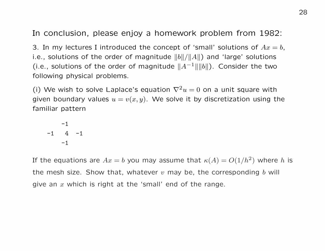
In conclusion, please enjoy a homework problem from 1982:

3. In my lectures I introduced the concept of ‘small’ solutions of Ax = b,

i.e., solutions of the order of magnitude ‖b‖/‖A‖) and ‘large’ solutions

(i.e., solutions of the order of magnitude ‖A−1‖‖b‖). Consider the two

following physical problems.

(i) We wish to solve Laplace’s equation ∇2u = 0 on a unit square with

given boundary values u = v(x, y). We solve it by discretization using the

familiar pattern

-1

-1 4 -1

-1

If the equations are Ax = b you may assume that κ(A) = O(1/h2) where h is

the mesh size. Show that, whatever v may be, the corresponding b will

give an x which is right at the ‘small’ end of the range.

29

(ii) We now wish to solve Poisson’s equation ∇2u = ρ with u = 0 on the

boundary. Assuming that ρ(x, y) is a ‘reasonably sensible function’, show

that b is such that as h → 0 the corresponding x is right at the ‘large’ end

of the range.

(iii) Can you explain how it is in (i) that x is always ‘small’ although v is

arbitrary?

(iv) What is the flaw in the following argument in connexion with (i):

(a) The computed solution is the solution of (A+ δA)x = b with

‖δA‖ ≤ ǫf(n)‖A‖, where f(n) is rather unimportant.

(b) r = b−Ax = δAx . Hence ‖r‖ ≤ ‖δA‖ ‖x‖.

(c) x is at the small end and hence ‖x‖ = O(‖b‖/‖A‖).

(d) Hence ‖r‖ = O(‖δA‖ ‖b‖/‖A‖), i.e., O(ǫf(n)‖b‖).

(Don’t be too critical about the use of O(·), that is not the point at issue.

(e) The elements of ‖b‖ come directly from the boundary values v and

hence we have the exact solution of a problem with boundary values v very

close to v (i.e., with ‖v − v‖ independent of κ(A)).

30

(v) For problem (i) defining r to be b−Ax, what is the discretized physical

problem to which we do have the exact solution? (You may describe this

physical problem in terms of the components ri of r.)

(vi) If X is the correctly rounded inverse of A, how good would Xb be for

problems (i) and (ii) respectively as regards accuracy? (Since A−1 is not

sparse, the efficiency is not good anyway.)

31

Here is Jim’s solution to problem 3 in Homework 2, Winter1982.

3.

v1 v2 v3 v4

v16 1 2 3 4 v5

v15 5 6 7 8 v6

v14 9 10 11 12 v7

v13 13 14 15 16 v8

v12 v11 v10 v9

(i) For Laplace’s equation we see that for an internal point typically

4x6 − x5 − x2 − x7 − x10 = 0.

An internal value could not therefore be greater than all other values. The

maximum is therefore achieved at a boundary point. For boundary points

we have typically

4x5 − x1 − x6 − x9 = v15 (non-corner point)

4x1 − x2 − x5 = v1 + v16 (corner point).

32

Obviously xi < max(vi) (∀i, j). This is the discretized version of the

maximum principle. Similarly, xi > min(vj) (∀i, j). This means

‖x‖∞ ≤ ‖v‖∞ = ‖b‖∞.

Hence, however irregular the boundary values may be, ‖x‖∞ is tied down

by ‖b‖ although ‖A−1‖ = O(1/h2) → ∞ as h → 0. The solution is right at

the small end.

(ii) For Poisson’s equation the R.H.S. corresponding to point ’i’ is

h2ρ(x, y) at that point. However, as h → 0, the solution x → solution of the

continuous problem, i.e., for a given function ρ(x, y) it is tending to a fixed

function u(x, y). But ‖b‖∞ = O(h2) and ‖A−1‖ = O(1/h2). The solution is

O(1) i.e., O(‖A−1‖‖b‖). The solution is right up at the large end.

(iii) Although v is quite arbitrary the R.H.S. of the system of equations is

always very special. If 1/h = n+ 1 we have n2 equations and for (n− 2)2 of

these the R.H.S. element is zero. It is therefore not at all surprising that if

b is expanded in terms of the eigenvectors of A, those corresponding to

the small eigenvalues (eigenvalues are singular values here because A is

positive definite) are absent. You will find it instructive to look at these

vectors and to see that b is deficient in them.

33

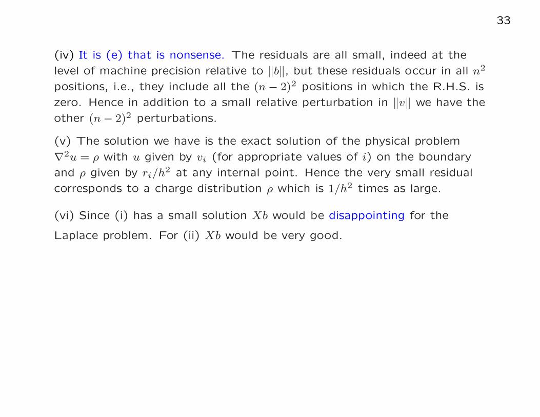
(iv) It is (e) that is nonsense. The residuals are all small, indeed at the

level of machine precision relative to ‖b‖, but these residuals occur in all n2

positions, i.e., they include all the (n− 2)2 positions in which the R.H.S. is

zero. Hence in addition to a small relative perturbation in ‖v‖ we have the

other (n− 2)2 perturbations.

(v) The solution we have is the exact solution of the physical problem

∇2u = ρ with u given by vi (for appropriate values of i) on the boundary

and ρ given by ri/h2 at any internal point. Hence the very small residual

corresponds to a charge distribution ρ which is 1/h2 times as large.

(vi) Since (i) has a small solution Xb would be disappointing for the

Laplace problem. For (ii) Xb would be very good.