lectures notes for mathematical theory of maxwell's equations
DESCRIPTION
MatemáticaTRANSCRIPT

Lecture Notes for
Mathematical Theory of Maxwell’s Equations
Sommer Term 2009
Prof. Dr. Andreas Kirsch
Department of MathematicsUniversity of Karlsruhe
1

Contents
1 Introduction 5
1.1 Maxwell’s Equations . . . . . . . . . . . . . . . . . . . . . . . . . . . . . . . . . . . . 5
1.2 The Constitutive Equations . . . . . . . . . . . . . . . . . . . . . . . . . . . . . . . . 7
1.3 Special Cases . . . . . . . . . . . . . . . . . . . . . . . . . . . . . . . . . . . . . . . . 8
1.3.1 Vacuum . . . . . . . . . . . . . . . . . . . . . . . . . . . . . . . . . . . . . . . 8
1.3.2 Electrostatics . . . . . . . . . . . . . . . . . . . . . . . . . . . . . . . . . . . . 9
1.3.3 Magnetostatics . . . . . . . . . . . . . . . . . . . . . . . . . . . . . . . . . . . 9
1.3.4 Time Harmonic Fields . . . . . . . . . . . . . . . . . . . . . . . . . . . . . . . 9
1.4 Boundary and Transmission Conditions . . . . . . . . . . . . . . . . . . . . . . . . . . 12
1.5 Vector Calculus . . . . . . . . . . . . . . . . . . . . . . . . . . . . . . . . . . . . . . . 15
1.5.1 Table of Differential Operators and Their Properties . . . . . . . . . . . . . . . 15
1.5.2 Elementary Facts from Differential Geometry, Integral Identities . . . . . . . . 17
2 Potentials of Time Harmonic Electromagnetic Fields 23
2.1 Representation Theorems . . . . . . . . . . . . . . . . . . . . . . . . . . . . . . . . . . 23
2.2 Smoothness of Potentials . . . . . . . . . . . . . . . . . . . . . . . . . . . . . . . . . . 33
2.2.1 The Scalar Volume and Surface Potentials . . . . . . . . . . . . . . . . . . . . 33
2.2.2 Vector Potentials . . . . . . . . . . . . . . . . . . . . . . . . . . . . . . . . . . 49
3 Electromagnetic Scattering From a Perfect Conductor 51
3.1 Formulation of the Problem and Uniqueness . . . . . . . . . . . . . . . . . . . . . . . 51
3.2 An Integral Equation and Mapping Properties of Some Boundary Operators . . . . . 56
3.3 Existence of Solutions of the Exterior Boundary Value Problem . . . . . . . . . . . . 63
4 The Variational Approach to the Cavity Problem 70
4.1 Sobolev Spaces of Scalar Functions . . . . . . . . . . . . . . . . . . . . . . . . . . . . 70
4.2 Sobolev Spaces of Vector Valued Functions . . . . . . . . . . . . . . . . . . . . . . . . 81
4.3 The Cavity Problem . . . . . . . . . . . . . . . . . . . . . . . . . . . . . . . . . . . . 86
4.4 Uniqueness and Unique Continuation . . . . . . . . . . . . . . . . . . . . . . . . . . . 90
5 Scattering by an Inhomogeneous Medium 101
2

3
Literature:
• P. Monk, Finite Element Methods for Maxwell’s Equation, Oxford University Press, 2003
• C. Muller, Foundations of the Theory of Electromagnetic Waves, Springer Verlag, Berlin 1969,(German original: 1957)
• D. Colton and R. Kress, Integral Equation Methods in Scattering Theory, Wiley-IntersciencePublication, New York 1983.
• D. Colton and R. Kress, Inverse Acoustic and Electromagnetic Scattering Theory, (2nd Edition)Springer, New York 1998.
• J.C. Nedelec: Acoustic and Electromagnetic Equations, Springer, New York, 2001.
More literature will be given during the course.
4

1 Introduction
1.1 Maxwell’s Equations
Electromagnetic wave propagation is described by particular equations relating five vector fields E ,D, H, B, J and the scalar field ρ, where E and D denote the electric field (in V/m) and electricdisplacement (in As/m2) respectively, while H and B denote the magnetic field (in A/m) andmagnetic flux density (in V s/m2 = T =Tesla). Likewise, J and ρ denote the current density(in A/m2) and charge density (in As/m3) of the medium. Here and throughout the lecture we usethe rationalized MKS-system, i.e. V , A, m and s. All fields will be assumed to depend both onthe space variable x ∈ R3 and on the time variable t ∈ R.
The actual equations that govern the behavior of the electromagnetic field, first completely formulatedby Maxwell, may be expressed easily in integral form. Such a formulation has the advantage of beingclosely connected to the physical situation. The more familiar differential form of Maxwell’s equationscan be derived very easily from the integral relations as we will see below.
In order to write these integral relations, we begin by letting S be a connected smooth surface withboundary ∂S in the interior of a region Ω0 where electromagnetic waves propagate. In particular,we require that the unit normal vector ν(x) for x ∈ S be continuous and directed always into “oneside” of S, which we call the positive side of S. By τ(x) we denote the unit vector tangent to theboundary of S at x ∈ ∂S. This vector, lying in the tangent plane of S together with a vector n(x),x ∈ ∂S, normal to ∂S is oriented so as to form a mathematically positive system (i.e. τ is directedcounterclockwise when we sit on the positive side of S, and n(x) is directed to the outside of S).Furthermore, let Ω ∈ R3 be an open set with boundary ∂Ω and outer unit normal vector ν(x) atx ∈ ∂Ω. Then Maxwell’s equations in integral form state:∫
∂S
H · τ d` =d
dt
∫S
D · ν dS +
∫S
J · ν dS (Ampere’s Law) (1.1a)
∫∂S
E · τ d` = − d
dt
∫S
B · ν dS (Law of Induction) (1.1b)
∫∂Ω
D · ν dS =
∫∫Ω
ρ dV (Gauss’ Electric Law) (1.1c)
∫∂Ω
B · ν dS = 0 (Gauss’ Magnetic Law) (1.1d)
To derive the Maxwell’s equations in differential form we consider a region Ω0 where µ and ε areconstant (homogeneous medium) or at least continuous. In regions where the vector fields aresmooth functions we can apply the Stokes and Gauss theorems for surfaces S and solids Ω lying
5
completely in Ω0: ∫S
curlF · ν dS =
∫∂S
F · τ d` (Stokes), (1.2)
∫∫Ω
div F dV =
∫∂Ω
F · ν dS (Gauss), (1.3)
where F denotes one of the fields H, E , B or D. We recall the differential operators (in cartesiancoordinates):
div F(x) =3∑
j=1
∂Fj
∂xj
(x) (divergenz, “Divergenz”)
curlF(x) =
∂F3
∂x2
(x)− ∂F2
∂x3
(x)
∂F1
∂x3
(x)− ∂F3
∂x1
(x)
∂F2
∂x1
(x)− ∂F1
∂x2
(x)
(curl, “Rotation”) .
With these formulas we can eliminate the boundary integrals in (1.1a-1.1d). We then use the factthat we can vary the surface S and the solid Ω in D arbitrarily. By equating the integrands we areled to Maxwell’s equations in differential form so that Ampere’s Law, the Law of Induction andGauss’ Electric and Magnetic Laws, respectively, become:
∂B∂t
+ curlx E = 0 (Faraday’s Law of Induction, “Induktionsgesetz”)
∂D∂t
− curlx H = −J (Ampere’s Law, “Durchflutungsgesetz”)
divx D = ρ (Gauss’ Electric Law, “Coulombsches Gesetz”)
divx B = 0 (Gauss’ Magnetic Law)
We note that the differential operators are always taken w.r.t. the spacial variable x (not w.r.t. timet!). Therefore, in the following we often drop the index x.
Physical remarks:
• The law of induction describes how a time-varying magnetic field effects the electric field.
• Ampere’s Law describes the effect of the current (external and induced) on the magnetic field.
• Gauss’ Electric Law describes the sources of the electric displacement.
6

• The forth law states that there are no magnetic currents.
• Maxwell’s equations imply the existence of electromagnetic waves (as ligh, X-rays, etc) invacuum and explain many electromagnetic phenomena.
• Literature wrt physics: J.D. Jackson, Klassische Elektrodynamik, de Gruyter Verlag
Historical Remark:
• Dates: Andre Marie Ampere (1775–1836), Charles Augustin de Coulomb (1736–1806), MichaelFaraday (1791–1867), James Clerk Maxwell (1831–1879)
• It was the ingeneous idea of Maxwell to modify Ampere’s Law which was known up to that timein the form curl H = J for stationary currents. Furthermore, he collected the four equationsas a consistent theory to describe the electromagnetic fields. (James Clerk Maxwell, Treatiseon Electricity and Magnetism, 1873).
Conclusion 1.1 Gauss’ Electric Law and Ampere’s Law imply the equation of continuity
∂ρ
∂t= div
∂D∂t
= div(curl H−J
)= −div J
since div curl = 0.
1.2 The Constitutive Equations
In this general setting the equation are not yet consistent (more unknown than equations). TheConstitutive Equations couple them:
D = D(E ,H) and B = B(E ,H)
The electric properties of material are complicated. In general, they not only depend on the molecularcharacter but also on macroscopic quantities as density and temperature of the material. Also, thereare time-dependent dependencies as, e.g., the hysteresis effect, i.e. the fields at time t depend alsoon the past.
As a first approximation one starts with representations of the form
D = E + 4πP and B = H− 4πM
where P denotes the electric polarisation vector and M the magnetization of the material. Thesecan be interpreted as mean values of microscopic effects in the material. Analogously, ρ and J aremacroskopic mean values of the free charge and current densities in the medium.
If we ignore ferro-electric and ferro-magnetic media and if the fields are small one can model thedependencies by linear equations of the form
D = εE and B = µH
7
with matrix-valued functions ε : R3 → R3×3 (dielectric tensor), and µ : R3 → R3×3 (permeabilitytensor). In this case we call the media inhomogenous and anisotropic.
The special case of an isotropic medium means that polarization and magnetisation do not dependon the directions. In this case they are just real valued functions, and we have
D = εE and B = µHwith functions ε, µ : R3 → R.
In the simplest case these functions ε and µ are constant. This is the case, e.g., in vacuum.
We indicated already that also ρ and J can depend on the material and the fields. Therefore,we need a further equation. In conducting media the electric field induces a current. In a linearapproximation this is described by Ohm’s Law:
J = σE + Je
where Je is the external current density. For isotropic media the function σ : R3 → R is called theconductivity.
Remark: If σ = 0 the the material is called dielectric. In vacuum we have σ = 0, ε = ε0 ≈8.854 · 10−12AS/V m, µ = µ0 = 4π · 10−7V s/Am. In anisotropic media, also the function σ is matrixvalued.
1.3 Special Cases
1.3.1 Vacuum
In regions of vacuum with no charge distributions and (external) currents (i.e. (ρ = 0,Je = 0) thelaw of induction takes the form
µ0∂H∂t
+ curl E = 0 .
Differentiation wrt time t and use of Ampere’s Law yields
µ0∂2H∂t2
+1
ε0
curl curl H = 0 ,
i.e.
ε0µ0∂2H∂t2
+ curl curl H = 0 .
1/√ε0µ0 has the dimension of velocity and is called the speed of light: c0 =
√ε0µ0.
From curl curl = ∇div − ∆ it follows that the components of H are solutions of the linear waveequation
c20∂2H∂t2
− ∆H = 0 .
Analogously, one derives the same equation for the electric field:
c20∂2E∂t2
− ∆E = 0 .
Remark: Heinrich Rudolf Hertz (1857–1894) showed also experimentally the existence of electro-magenetic waves about 20 years after Maxwell’s paper (in Karlsruhe!).
8

1.3.2 Electrostatics
If E is in some region Ω constant wrt time t (i.e. in the static case) the law of induction reduces to
curl E = 0 in Ω .
Therefore, if Ω is simply connected there exists a potential u : Ω → R with E = −∇u in Ω. Gauss’Electric Law yields in homogeneous media the Poisson equation
ρ = div D = −div (ε0E) = −ε0∆u
for the potential u. The electrostatics is described by this basic elliptic partial differential equation∆u = −ρ/ε0. Mathematically, this is the subject of potential theory.
1.3.3 Magnetostatics
The same technique does not work in magnetostatics since, in general, curl H 6= 0. However, since
div B = 0
we conclude the existence of a vector potential A : R3 → R3 with B = −curl A in D. Substitutingthis into Ampere’s Law yields (for homogeneous media Ω) after multiplication with µ0
−µ0J = curl curl A = ∇div A − ∆A .
Since curl∇ = 0 we can add gradients ∇u to A without changing B. We will see later that we canchoose u such that the resulting potential A satisfies div A = 0. This choice of normalization iscalled Coulomb gauge.
With this normalization we also get in the magnetostatic case the Poisson equation
∆A = −µ0J .
We note that in this case the Laplacian has to be taken component wise.
1.3.4 Time Harmonic Fields
Under the assumptions that the fields allow a Fourier transformation w.r.t. time we set
E(x;ω) = (FtE)(x;ω) =
∫R
E(x, t) eiωt dt ,
H(x;ω) = (FtH)(x;ω) =
∫R
H(x, t) eiωt dt ,
etc. We note that the fields E, H etc are now complex valued, i.e, E(·;ω), H(·;ω) : R3 → C3
(and also the other fields). Although they are vector fields we denote them by capital Latin letters
9

only. Maxwell’s equations transform into (since Ft(u′) = −iωFtu) the time harmonic Maxwell’s
equations
−iωB + curlE = 0 ,
iωD + curlH = σE + Je ,
divD = ρ ,
divB = 0 .
Remark: The time harmonic Maxwell’s equation can also be derived from the assumption that allfields behave periodically w.r.t. time with the same frequency ω. Then the forms E(x, t) = e−iωtE(x),H(x, t) = e−iωtH(x), etc satisfy the time harmonic Maxwell’s equations. With the constitutiveequations D = εE and B = µH we arrive at
−iωµH + curlE = 0 , (1.4a)
iωεE + curlH = σE + Je , (1.4b)
div (εE) = ρ , (1.4c)
div (µH) = 0 . (1.4d)
Eliminating H or E, respectively, from (1.4a) and (1.4b) yields
curl
(1
iωµcurlE
)+ (iωε− σ)E = Je . (1.5)
and
curl
(1
iωε− σcurlH
)+ iωµH = curl
(1
iωε− σJe
), (1.6)
respectively. Usually, one writes these equations in a slightly different way by introducing the constantvalues ε0 > 0 and µ0 > 0 in vacuum and relative values (dimensionless!) εr ∈ C and µr ∈ R, definedby
εr =1
ε0
(ε +
iσ
ω
), µr =
µ
µ0
.
Then equations (1.5) and (1.6) take the form
curl
(1
µr
curlE
)− k2εr E = iωµ0Je , (1.7)
curl
(1
εr
curlH
)− k2µr H = curl
(1
εr
Je
), (1.8)
with the wave number k = ω√ε0µ0. In vacuum we have εr = 1, µr = 1 and thus
curl curlE − k2E = iωµ0Je , (1.9)
curl curlH − k2H = curl Je . (1.10)
10
Example 1.2 In the case Je = 0 and in vacuum the fields
E(x) = p eik d·x and H(x) = (p× d) eik d·x
are solutions of the time harmonic Maxwell’s equations (1.9), (1.10) provided d is a unit vector inR3 and p ∈ C3 with p · d = 01. Such fields are called plane time harmonic fields with polarizationvector p ∈ C3 and direction d.
We make the assumption εr = 1, µr = 1 for the rest of Section 1.3. Taking the divergence of theseequations yield divH = 0 and k2divE = −iωµ0div Je, i.e. divE = −(i/ωε0)div Je. Comparing thisto (1.4c) yields the time harmonic version of the equation of continuity
div Je = iωρ .
With the vector identity curl curl = −∆ + div∇ equations (1.10) and (1.9) can be written as
∆E + k2E = −iωµ0Je +1
ε0
∇ρ , (1.11)
∆H + k2H = −curl Je . (1.12)
We consider the magnetic field first and introduce magnetic Hertz potentials: divH = 0 impliesthe existence of a vector potential A with H = curlA. Thus (1.12) takes the form
curl (∆A + k2A) = −curl Je
and thus∆A + k2A = −Je + ∇ϕ (1.13)
for some scalar field ϕ. On the other hand, if A and ϕ satisfy (1.13) then
H = curlA and E = − 1
iωε0
(curlH − Je) = iωµ0A − 1
iωε0
∇(divA− ϕ)
satisfies the Maxwell system (1.4a)–(1.4d).
Analogously, we can introduce electric Hertz potentials if Je = 0. Since then divE = 0 thereexists a vector potential A with E = curlA. Substituting this into (1.11) yields
curl (∆A + k2A) = 0
and thus∆A + k2A = ∇ϕ (1.14)
for some scalar field ϕ. On the other hand, if A and ϕ satisfy (1.14) then
E = curlA and H =1
iωµ0
curlE = −iωε0A +1
iωµ0
∇(divA− ϕ)
satifies the Maxwell system (1.4a)–(1.4d).
1We set p · d =∑3
j=1 pjdj even for p ∈ C3
11

As a particular example we take the magnetic Hertz vector A of the form A(x) = u(x) z with a scalarfunction u and the uni vector z = (0, 0, 1)> ∈ R3. Then
H = curl (uz) =
(∂u
∂x2
,− ∂u
∂x1
, 0
)>
,
E = iωµ0 z +1
−iωε0
∇(∂u/∂x3) .
If u is independent of x3 then E has only a x3−component and this mode is called E-mode orTM-mode (for transverse-magnetic). Analogously, the H-mode or TE-mode is defined. In anycase, the vector Helmholtz equation for A reduced to the scalar Helmholtz equation for u.
1.4 Boundary and Transmission Conditions
Maxwell’s equations hold only in regions with smooth parameter functions εr, µr and σ. If weconsider a situation in which a surface S separates two homogeneous media from each other, theconstitutive parameters ε, µ and σ are no longer continuous but piecewise continuous with finitejumps on S. While on both sides of S Maxwell’s equations (1.4a)–(1.4d) hold, the presence of thesejumps implies that the fields satisfy certain conditions on the surface.
To derive the mathematical form of this behaviour (the boundary conditions) we apply the law ofinduction (1.1b) to a narrow rectangle-like surface R, containing the normal n to the surface S andwhose long sides C+ and C− are parallel to S and are on the opposite sides of it, see the followingfigure.
12

When we let the height of the narrow sides, AA′ and BB′, approach zero then C+ and C− approacha curve C on S, the surface integral ∂
∂t
∫R
B · ν dS will vanish in the limit since the field remainsfinite (note, that the normal ν is the normal to R lying in the tangential plane of S). Hence, the lineintegrals
∫C
E+ · τ d` and∫
CE− · τ d` must be equal. Since the curve C is arbitrary the integrands
E+ · τ and E− · τ coincide on every arc C, i.e.
n× E+ − n× E− = 0 on S . (1.15)
A similar argument holds for the magnetic field in (1.1a) if the current distribution J = σE + Je
remains finite. In this case, the same arguments lead to the boundary condition
n×H+ − n×H− = 0 on S . (1.16)
If, however, the external current distribution is a surface current, i.e. if Je is of the form Je(x +τn(x)) = Js(x)δ(τ) for small τ and x ∈ S and with tangential surface field Js and σ is finite, thenthe surface integral
∫R
Je · ν dS will tend to∫
CJs · ν d`, and so the boundary condition is
n×H+ − n×H− = Js on S . (1.17)
We will call (1.15) and (1.16) or (1.17) the transmission boundary conditions.
A special and very important case is that of a perfectly conducting medium with boundary S.Such a medium is characterized by the fact that the electric field vanishes inside this medium, and(1.15) reduces to
n× E = 0 on S (1.18)
Another important case is the impedance- or Leontovich boundary condition
n×H = λn× (E × n) on S (1.19)
which, under appropriate conditions, may be used as an approximation of the transmission conditions.
The same kind of boundary occur also in the time harmonic case (where we denote the fields bycapital Latin letters).
Finally, we specify the boundary conditions to the E- and H-modes derived above. We assume thatthe surface S is an infinite cylinder in x3−direction with constant cross section. Furthermore, weassume that the volume current density J vanishes near the boundary S and that the surface currentdensities take the form Js = jsz for the E-mode and Js = js
(ν × z
)for the H-mode. We use the
notation [v] := v|+ − v|− for the jump of the function v at the boundary. Also, we abbreviate (onlyfor this table) σ′ = σ − iωε. We list the boundary conditions in the following table.
Boundary condition E-mode H-mode
transmission [u] = 0 on S ,[µ ∂u
∂ν
]= 0 on S ,[
σ′ ∂u∂ν
]= −js on S , [u] = js on S ,
impedance λ k2u+ σ′ ∂u∂ν
= −js on S , k2u− λ iωµ∂u∂ν
= js on S ,
perfect conductor u = 0 on S , ∂u∂ν
= 0 on S .
13

The situation is different for the normal components. We consider Gauss’ Electric and MagneticLaws and choose Ω to be a box which is separated by S into two parts Ω1 and Ω2. We apply (1.1c)first to all of Ω and then to Ω1 and Ω2 separately. The addition of the last two formulas and thecomparison with the first yields that the normal component D · n has to be continuous as well as(application of (1.1d)) B · n. With the constitutive equations one gets
n · (εr,1E1 − εr,2E2) = 0 on S and n · (µr,1H1 − µr,2H2) = 0 on S .
Conclusion 1.3 The normal components of E and/or H are not continuous at interfaces where εr
and/or µr have jumps.
During our course we will consider two classical boundary value problems.
• (Cavity with an ideal conductor as boundary) Let D ⊆ R3 be a bounded domainwith sufficiently smooth boundary ∂D and exterior unit normal vector ν(x) at x ∈ ∂D. LetF : D → C3 be a smooth vector field. Determine a solution E ∈ C2(D) ∩ C(D) of the timeharmonic Maxwell’s equation
curl
(1
µr
curlE
)− k2εrE = F in D ,
such thatν × E = 0 on ∂D .
D
εr, µr
ν × E = 0
• (Scattering by an inhomogeneous medium) Given µr, εr ∈ L∞(R3) with µr = εr = 1outside some bounded region D and some solution Ei and H i of the “unperturbed” timeharmonic Maxwell system
curlEi − iµ0Hi = 0 in R3 , curlH i + iε0E
i = 0 in R3 ,
determine E,H of the perturbed Maxwell system
curlE − iµ0µrH = 0 in R3 , curlH + iε0εrE = 0 in R3 ,
14

such that E and H satisisfy the transmission conditions (1.15) and (1.16), and E and H havethe decompositions into E = Es +Ei and H = Hs +H i in R3 with some scattered field Es, Hs
which satisfy the Silver-Muller radiation condition
lim|x|→∞
|x|(Hs(x)× x
|x|−
√ε0
µ0
Es(x)
)= 0
lim|x|→∞
|x|(Es(x)× x
|x|+
õ0
ε0
Hs(x)
)= 0
uniformly with respect to all directions x/|x|.
Remark: For general µr, εr ∈ L∞(R3) we have to give a correct interpretation of the differentialequations (“variational or weak formulation”) and transmission conditions (“trace theorems”).
D
εr, µr
ε0, µ0, σ = 0
Ei, H i
AAAAAA
AA
AA
AA
HHHHHHj Es, Hs
1.5 Vector Calculus
In this subsection we collect the most important formulas from vector calculus.
1.5.1 Table of Differential Operators and Their Properties
We assume that all functions are sufficiently smooth. In cartesian coordinates:
15
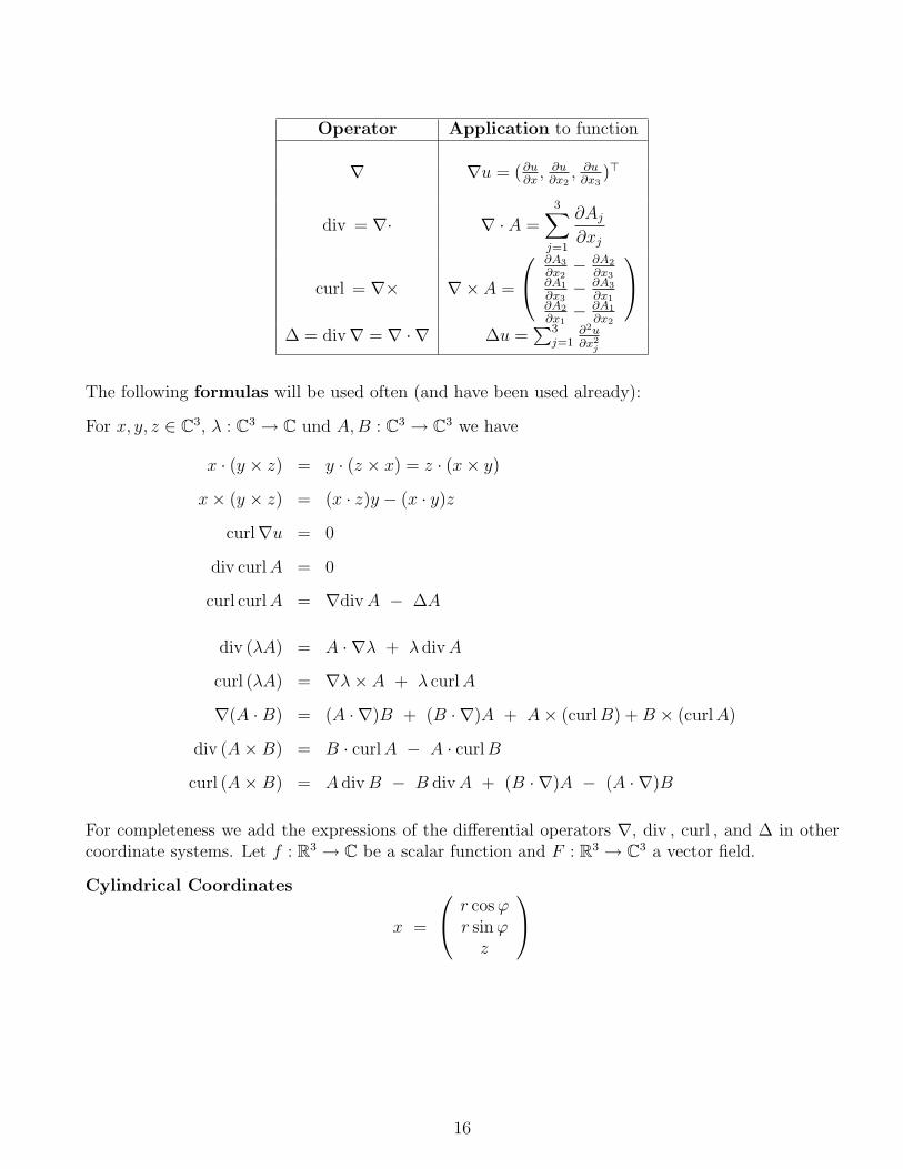
Operator Application to function
∇ ∇u = (∂u∂x, ∂u
∂x2, ∂u
∂x3)>
div = ∇· ∇ · A =3∑
j=1
∂Aj
∂xj
curl = ∇× ∇× A =
∂A3
∂x2− ∂A2
∂x3∂A1
∂x3− ∂A3
∂x1∂A2
∂x1− ∂A1
∂x2
∆ = div∇ = ∇ · ∇ ∆u =
∑3j=1
∂2u∂x2
j
The following formulas will be used often (and have been used already):
For x, y, z ∈ C3, λ : C3 → C und A,B : C3 → C3 we have
x · (y × z) = y · (z × x) = z · (x× y)
x× (y × z) = (x · z)y − (x · y)z
curl∇u = 0
div curlA = 0
curl curlA = ∇divA − ∆A
div (λA) = A · ∇λ + λ divA
curl (λA) = ∇λ× A + λ curlA
∇(A ·B) = (A · ∇)B + (B · ∇)A + A× (curlB) +B × (curlA)
div (A×B) = B · curlA − A · curlB
curl (A×B) = A divB − B divA + (B · ∇)A − (A · ∇)B
For completeness we add the expressions of the differential operators ∇, div , curl , and ∆ in othercoordinate systems. Let f : R3 → C be a scalar function and F : R3 → C3 a vector field.
Cylindrical Coordinates
x =
r cosϕr sinϕz
16

Let z = (0, 0, 1)> and r = (cosϕ, sinϕ, 0)> and ϕ = (− sinϕ, cosϕ, 0)> be the coordinate unitvectors. Let F = Frr + Fϕϕ+ Fz z. Then
∇f(r, ϕ, z) =∂f
∂rr +
1
r
∂f
∂ϕϕ +
∂f
∂zz ,
divF (r, ϕ, z) =1
r
∂(rFr)
∂r+
1
r
∂Fϕ
∂ϕ+
∂Fz
∂z,
curlF (r, ϕ, z) =
(1
r
∂Fz
∂ϕ− ∂Fϕ
∂z
)r +
(∂Fr
∂z− ∂Fz
∂r
)ϕ +
1
r
(∂(rFϕ)
∂θ− ∂Fθ
∂ϕ
)z ,
∆f(r, ϕ, z) =1
r
∂
∂r
(r∂f
∂r
)+
1
r2
∂2f
∂ϕ2+
∂2f
∂z2.
Spherical Coordinates
x =
r sin θ cosϕr sin θ sinϕr cos θ
Let r = (sin θ cosϕ, sin θ sinϕ, cos θ)> and θ = (cos θ cosϕ, cos θ sinϕ,− sin θ)> andϕ = (− sin θ sinϕ, sin θ cosϕ, 0)> be the coordinate unit vectors. Let F = Frr + Fθθ + Fϕϕ. Then
∇f(r, θ, ϕ) =∂f
∂rr +
1
r
∂f
∂θθ +
1
r sin θ
∂f
∂ϕϕ ,
divF (r, θ, ϕ) =1
r2
∂(r2Fr)
∂r+
1
r sin θ
∂(sin θ Fθ)
∂θ+
1
r sin θ
∂Fϕ
∂ϕ,
curlF (r, θ, ϕ) =1
r sin θ
(∂(sin θ Fϕ)
∂θ− ∂Fθ
∂ϕ
)r +
1
r
(1
sin θ
∂Fr
∂ϕ− ∂(rFϕ)
∂r
)θ +
+1
r
(∂(rFθ)
∂r− ∂Fr
∂θ
)ϕ ,
∆f(r, θ, ϕ) =1
r2
∂
∂r
(r2∂f
∂r
)+
1
r2 sin θ
∂
∂θ
(sin θ
∂f
∂θ
)+
1
r2 sin2 θ
∂2f
∂ϕ2.
1.5.2 Elementary Facts from Differential Geometry, Integral Identities
Before we recall the basic integral identity of Gauss and Green we have to define rigourously thenotion of domain with Cn−boundaries. We denote by K(x, r) := Kj(x, r) := y ∈ Rj : |y − x| < rand K[x, r] := Kj[x, r] := y ∈ Rj : |y − x| ≤ r the open and closed ball of radius r > 0 centeredat x in Rj for j = 2 or 3.
Definition 1.4 We call a region D ⊂ R3 to be Cn-smooth (i.e. D ∈ Cn), if there exists a finitenumber of open sets Uj ⊂ R3, j = 1, . . . ,m, and bijective mappings Ψj from the closed unit ballK3[0, 1] := u ∈ R3 : |u| ≤ 1 onto U j such that
17

(i) ∂D ⊂m⋃
j=1
Uj,
(ii) Ψj ∈ Cn(K[0, 1]) and Ψ−1j ∈ Cn(U j) for all j = 1, . . . ,m,
(iii) det Ψ′j(u) 6= 0 for all |u| ≤ 1, j = 1, . . . ,m, where Ψ′
j(u) ∈ R3×3 denotes the Jacobian of Ψj atu,
(iv) it holds that
Ψ−1j (Uj ∩D) = u ∈ R3 : |u| < 1, u3 > 0 ,
Ψ−1j (Uj ∩ ∂D) = u ∈ R3 : |u| < 1, u3 = 0 .
The restriction Ψj of the mapping Ψj to K2[0, 1]×0 ⊂ K3[0, 1] yields a parametrization of ∂D∩Uj
in the form x = Ψj(u) = Ψj(u1, u2, 0), u ∈ K2[0, 1].If Ψ is one of the mappings Ψj then ∂Ψ
∂u1(u) and ∂Ψ
∂u2(u), are tangential vectors at x = Ψ(u). They are
linearly independent since det Ψ′(u1, u2, 0) 6= 0 and, therefore, span the tangent plane at x = Ψ(u).The unit vectors
ν(x) = ±∂Ψ∂u1
(u)× ∂Ψ∂u2
(u)∣∣∣ ∂Ψ∂u1
(u)× ∂Ψ∂u2
(u)∣∣∣
for x = Ψ(u) ∈ ∂D ∩ Uj are orthogonal to the the tangent plane, thus normal vectors. The signis chosen such that ν(x) is directed into the exterior of D (i.e. x + tν(x) ∈ Uj \ D for smallt > 0). The unit vector ν(x) is called the exterior unit normal vector. For such domains andcontinuous functions f : ∂D → C the surface integral
∫∂Df(x) dS exists. Using local coordinates
Ψj : K2(0, 1) → Uj ∩ ∂D the integral over the surface patch Uj ∩ ∂D is given by∫Uj∩∂D
f(x) dS =
∫K2(0,1)
f(Ψj(u)
) ∣∣∣∣∂Ψj
∂u1
(u)× ∂Ψj
∂u2
(u)
∣∣∣∣ du .We collect important properties of the smooth domain D in the following lemma.
Lemma 1.5 Let D ∈ C2. Then there exists c0 > 0 such that
(a)∣∣ν(y) · (y − z)
∣∣ ≤ c0|z − y|2 for all y, z ∈ ∂D,
(b)∣∣ν(y)− ν(z)
∣∣ ≤ c0|y − z| for all y, z ∈ ∂D.
(c) DefineHρ :=
z + tν(z) : z ∈ ∂D , |t| < ρ
.
Then there exists ρ0 > 0 such that for all ρ ∈ (0, ρ0] and every x ∈ Hρ there exist unique (!)z ∈ ∂D and |t| ≤ ρ with x = z + tν(z). The set Hρ is an open neighborhood of ∂D for everyρ ≤ ρ0. Furthermore, z − tν(z) ∈ D and z + tν(z) /∈ D for 0 < t < ρ and z ∈ ∂D.One can choose ρ0 such that for all ρ ≤ ρ0 the following holds:
• |z − y| ≤ 2|x− y| for all x ∈ Hρ and y ∈ ∂D, and
18

• |z1 − z2| ≤ 2|x1 − x2| for all x1, x2 ∈ Hρ.
If Uδ :=x ∈ R3 : infz∈∂D |x − z| < δ
denotes the strip around ∂D then there exists δ > 0
withUδ ⊂ Hρ0 ⊂ Uρ0 (1.20)
(d) There exists r0 > 0 such that the surface area of ∂K(z, r) ∩D for z ∈ ∂D can be estimated by∣∣|∂K(z, r) ∩D| − 2πr2∣∣ ≤ 4πc0 r
3 for all r ≤ r0 . (1.21)
Proof: We make use of a finite covering⋃Uj of ∂D, i.e. we write ∂D =
⋃(Uj ∩ ∂D) and use local
coordinates Ψj : R2 ⊃ K2[0, 1] → R3 which yields the parametrization of ∂D ∩ Uj. First, it is easyto see (proof by contradiction) that there exists δ > 0 with the property that for every pair (z, x) ∈∂D×R3 with |z − x| < δ there exists Uj with z, x ∈ Uj. Let diam(D) = sup
|x1 − x2| : x1, x2 ∈ D
be the diameter of D.(a) Let x, y ∈ ∂D and assume first that |y − x| ≥ δ. Then
∣∣ν(y) · (y − x)∣∣ ≤ |y − x| ≤ diam(D)
δ2δ2 ≤ diam(D)
δ2|y − x|2 .
Let now |y − x| < δ. Then there exists Uj with y, x ∈ Uj. Let x = Ψj(u) and y = Ψj(v). Then
ν(x) = ±∂Ψj
∂u1(u)× ∂Ψj
∂u2(u)∣∣∣∂Ψj
∂u1(u)× ∂Ψj
∂u2(u)
∣∣∣and, by the definition of the derivative,
y − x = Ψj(v)−Ψj(u) =2∑
k=1
(vk − uk)∂Ψj
∂uk
(u) + a(v, u)
with∣∣a(v, u)∣∣ ≤ c|u− v|2 for all u, v ∈ Uj and some c > 0. Therefore,
∣∣ν(x) · (y − z)∣∣ ≤ 1∣∣∣∂Ψj
∂u1(u)× ∂Ψj
∂u2(u)
∣∣∣2∑
k=1
(vk − uk)
∣∣∣∣(∂Ψj
∂u1
(u)× ∂Ψj
∂u2
(u)
)· ∂Ψj
∂uk
(u)
∣∣∣∣︸ ︷︷ ︸= 0
+1∣∣∣∂Ψj
∂u1(u)× ∂Ψj
∂u2(u)
∣∣∣∣∣∣∣(∂Ψj
∂u1
(u)× ∂Ψj
∂u2
(u)
)· a(v, u)
∣∣∣∣≤ c |u− v|2 = c
∣∣Ψ−1j (x)−Ψ−1
j (y)∣∣2 ≤ c0 |x− y|2 .
This proves part (a). The proof of (b) follows analogously from the differentiability of u 7→ ν.
(c) Choose ρ0 > 0 such that
(i) ρ0 c0 < 1/16 and
19

(ii) ν(x1) · ν(x2) ≥ 0 for x1, x2 ∈ ∂D with |x1 − x2| ≤ 2ρ0 and
(iii) Hρ0 ⊂⋃Uj.
Assume that x has two representation as x = z1 + t1ν1 = z2 + t2ν2 where we write νj for ν(zj). Then
|z1 − z2| =∣∣(t2 − t1) ν2 + t1 (ν2 − ν1)
∣∣ ≤ |t1 − t2| + ρ c0|z1 − z2| ≤ |t1 − t2| +1
16|z1 − z2| ,
thus |z1 − z2| ≤ 1615|t1 − t2| ≤ 2|t1 − t2|. Furthermore, since ν1 · ν2 ≥ 0,
(ν1 + ν2) · (z1 − z2) = (ν1 + ν2) · (t2ν2 − t1ν1) = (t2 − t1) (ν1 · ν2 + 1)︸ ︷︷ ︸≥1
,
thus|t2 − t1| ≤
∣∣(ν1 + ν2) · (z1 − z2)∣∣ ≤ 2c0|z1 − z2|2 ≤ 8c0|t1 − t2|2 ,
i.e. |t2 − t1|(1− 8c0|t2 − t1|
)≤ 0. This yields t1 = t2 since 1− 8c0|t2 − t1| ≥ 1− 16c0ρ > 0 and thus
also z1 = z2.
Let U be one of the sets Uj and Ψ : R2 ⊃ K2(0, 1) → U ∩ ∂D the corresponding bijective mapping.We define the new mapping F : R2 ⊃ K2(0, 1)× (−ρ, ρ) → Hρ by
F (u, t) = Ψ(u) + t ν(u) , (u, t) ∈ K2(0, 1)× (−ρ, ρ) .
For sufficiently small ρ the mapping F is one-to-one and satisfies∣∣detF ′(u, t)
∣∣ ≥ c > 0 on K2(0, 1)×(−ρ, ρ) for some c > 0. Indeed, this follows from
F ′(u, t) =
(∂Ψ
∂u1
(u) + t∂ν
∂u1
(u) ,∂Ψ
∂u2
(u) + t∂ν
∂u2
(u) , ν(u)
)>
and the fact that for t = 0 the matrix F ′(u, 0) has full rank 3. Therefore, F is a bijective mappingfrom K2(0, 1)× (−ρ, ρ) onto U ∩Hρ. Therefore, Hρ =
⋃(Hρ ∩ Uj) is an open neighborhood of ∂D.
This proves also that x = z − tν(z) ∈ D and x = z + tν(z) /∈ D for 0 < t < ρ.
For x = z + tν(z) and y ∈ ∂D we have
|x− y|2 =∣∣(z − y) + tν(z)
∣∣2 ≥ |z − y|2 + 2t(z − y) · ν(z)
≥ |z − y|2 − 2ρc0|z − y|2
≥ 1
4|z − y|2 since 2ρc0 ≤
3
4.
Therefore, |z − y| ≤ 2|x− y|. Finally,
|x1 − x2|2 =∣∣(z1 − z2) + (t1ν1 − t2ν2)
∣∣2 ≥ |z1 − z2|2 − 2∣∣(z1 − z2) · (t1ν1 − t2ν2)
∣∣≥ |z1 − z2|2 − 2 ρ
∣∣(z1 − z2) · ν1
∣∣ − 2 ρ∣∣(z1 − z2) · ν2
∣∣≥ |z1 − z2|2 − 4 ρ c0 |z1 − z2|2 = (1− 4ρc0) |z1 − z2|2 ≥ 1
4|z1 − z2|2
20

since 1− 4ρc0 ≥ 1/4.The proof of (1.20) is simple and left as an exercise.
(d) Let c0 and ρ0 as in parts (a) and (c). Choose r0 such that K[z, r] ⊂ Hρ0 for all r ≤ r0 (which ispossible by (1.20)) and ν(z1) · ν(z1) > 0 for |z1 − z2| ≤ 2r0. For fixed r ≤ r0 and arbitrary z ∈ ∂Dand σ > 0 we define
Z(σ) =x ∈ ∂K(z, r) : (x− z) · ν(z) ≤ σ
We show that
Z(−2c0r2) ⊂ ∂K(z, r) ∩D ⊂ Z(+2c0r
2)
Let x ∈ Z(−2c0r2) have the form x = x0 + tν(x0). Then
(x− z) · ν(z) = (x0 − z) · ν(z) + t ν(x0) · ν(z) ≤ −2c0r2 ,
i.e.
t ν(x0) · ν(z) ≤ −2c0r2 +
∣∣(x0 − z) · ν(z)∣∣ ≤ −2c0r
2 + c0|x0 − z|2
≤ −2c0r2 + 2c0|x− z|2 = 0 ,
i.e. t ≤ 0 since |x0 − z| ≤ 2r and thus ν(x0) · ν(z) > 0. This shows x = x0 + tν(x0) ∈ D.Analogously, for x = x0 − tν(x0) ∈ ∂K(z, r) ∩D we have t > 0 and thus
(x− z) · ν(z) = (x0 − z) · ν(z)− t ν(x0) · ν(z) ≤ c0|x0 − z|2 ≤ 2c0|x− z|2 = 2c0r2 .
Therefore, the surface area of ∂K(z, r) ∩ D is bounded from below and above by the surface areasof Z(−2c0r
2) and Z(+2c0r2), respectively. Since the surface area of Z(σ) is 2πr(r + σ) we have
−4πc0 r3 ≤ |∂K(z, r) ∩D| − 2πr2 ≤ 4πc0 r
3 .
2
Now we can formulate the mentioned integral identities. We do it only in R3. By Cn(D)3 we denotethe space of vector fields F : D → C3 which are n−times continuously differentiable. By Cn(D)3 wedenote the subspace of Cn(D)3 that consists of those functions F which, together with all derivativesup to order n, have continuous extentions to the closure D of D.
Theorem 1.6 (Theorem of Gauss, Divergence Theorem)
Let D ⊂ R3 be a bounded domain which is C2−smooth. For F ∈ C1(D)3 ∩ C(D)3 the identity∫∫D
divF (x) dV =
∫∂D
Fν(x) dS
holds. In particular, the integral on the left hand side exists.
As a conclusion one derives the theorems of Green.
21

Theorem 1.7 (Green’s first and second theorem)
Let D ⊂ R3 be a bounded domain which is C2−smooth. Furthermore, let u, v ∈ C2(D) ∩ C1(D).Then ∫∫
D
(u∆v +∇u · ∇v) dV =
∫∂D
u∂v
∂νdS ,∫∫
D
(u∆v −∆u v) dV =
∫∂D
(u∂v
∂ν− v
∂u
∂ν
)dS .
Here, ∂u(x)/∂ν = ν(x) · ∇u(x) for x ∈ ∂D.
Proof: The first identity is derived from the divergence theorem be setting F = u∇v. Then Fsatisfies the assumption of Theorem 1.6 and divF = u∆v +∇u · ∇v.The second identity is derived by interchanging the roles of u and v in the first identity and takingthe difference of the two formulas. 2
We will also need their vector valued analoga.
Theorem 1.8 (Integral identities for vector fields)Let D ⊂ R3 be a bounded domain which is C2−smooth. Furthermore, let A,B ∈ C1(D)3 ∩ C(D)3
and let u ∈ C2(D) ∩ C1(D). Then ∫∫D
curlAdV =
∫∂D
ν × AdS , (1.22a)∫∫D
(B · curlA− A · curlB) dV =
∫∂D
(ν × A) ·B dS , (1.22b)∫∫D
(u divA+ A · ∇u) dV =
∫∂D
u (ν · A) dS . (1.22c)
Proof: For the first identity we consider the components separately. For the first one we have
∫∫D
(curlA)1 dV =
∫∫D
(∂A3
∂x2
− ∂A2
∂x3
)dV =
∫∫D
div
0A3
−A2
dV
=
∫∂D
ν ·
0A3
−A2
dS =
∫∂D
(ν × A)1 dS .
For the other components it is proven in the same way.For the second equation we set F = A × B. Then divF = B · curlA − A · curlB and ν · F =ν · (A×B) = (ν × A) ·B.For the third identity we set F = uA and have divF = u divA+ A · ∇u and ν · F = u(ν · A). 2
22

2 Potentials of Time Harmonic Electromagnetic Fields
2.1 Representation Theorems
We begin with the (really!) fundamental solution of the Helmholtz equation.
Lemma 2.1 For k ∈ C the function Φk :(x, y) ∈ R3 × R3 : x 6= y
→ C, defined by
Φk(x, y) =eik|x−y|
4π|x− y|, x 6= y ,
is called the fundamental solution of the Helmholtz equation, i.e. it holds that
∆xΦk(x, y) + k2Φk(x, y) = 0 for x 6= y .
Proof: This is easy to check. 2
We often suppress the index k, i.e. write Φ for Φk.
Throughout this section we always assume that D is a bounded domain which is C2−smooth.Then the divergence theorem holds as well as Green’s identities.
We begin with the existence of certain special improper integrals.
Lemma 2.2 (a) Let K : (x, y) ∈ R3 × D : x 6= y→ C be continuous. Assume that there exists
c > 0 and β > 0 such that∣∣K(x, y)∣∣ ≤ c
|x− y|3−βfor all x ∈ R3 and y ∈ D with x 6= y .
Then∫∫
DK(x, y) dV (y) exists as an improper integral and there exists cβ > 0 with∫∫
D\K(x,τ)
∣∣K(x, y)∣∣ dV (y) ≤ cβ for all x ∈ R3 and all τ > 0 . (2.1a)
(b) Let K : (x, y) ∈ ∂D × ∂D : x 6= y→ C be continuous. Assume that there exists c > 0 and
β > 0 such that ∣∣K(x, y)∣∣ ≤ c
|x− y|2−βfor all x, y ∈ ∂D with x 6= y .
Then∫
∂DK(x, y) dS(y) exists as an improper integral and there exists cβ > 0 with∫
∂D\K(x,τ)
∣∣K(x, y)∣∣ dS(y) ≤ cβ for all x ∈ ∂D and τ > 0 . (2.1b)
23

Proof: (a) Fix x ∈ R3 and choose R > 0 such that D ⊂ K(0, R).First case: |x| ≤ 2R. Then D ⊂ K(x, 3R) and thus, using spherical polar coordinares w.r.t. x,∫∫
D\K(x,τ)
1
|x− y|3−βdV (y) ≤
∫∫τ<|y−x|<3R
1
|x− y|3−βdV (y) = 4π
3R∫τ
1
r3−βr2 dr
=4π
β
[(3R)β − τβ
]≤ 4π
β(3R)β .
Second case: |x| > 2R. Then |x− y| ≥ |x| − |y| ≥ R for y ∈ D and thus∫∫D\K(x,τ)
1
|x− y|3−βdV (y) ≤ 1
R3−β
∫∫K(0,R)
dV =1
R3−β
4π
3R3 .
(b) By covering ∂D with finitely many open sets Uj as in Definition 1.4 we can use local coordinatesy = Ψ(v), v ∈ K2(0, 1) ⊂ R2. Let x = Ψ(u). Since Ψ is an isomorphism and Ψ′ is regular we havean estimate of the form
c1|x− y| ≤ |u− v| ≤ c2|x− y| for all x, y ∈ U .
Therefore, using polar coordinates w.r.t. u,∫∂D
|x−y|>τ
dS(y)
|x− y|2−β≤ c2−β
2
∫K2(0,1)\K2(u,c1τ)
1
|u− v|2−β
∣∣∣∣∂Ψ
∂v1
(v)× ∂Ψ
∂v2
(v)
∣∣∣∣ dv≤ ‖Ψ′‖2
∞ c2−β2
∫K2(u,2)\K2(u,c1τ)
dv
|u− v|2−β
= ‖Ψ′‖2∞ c2−β
2 4π
2∫c1τ
1
r2−βr dr = ‖Ψ′‖2
∞4π c2−β
2
β
[2β − (c1τ)
β]
≤ ‖Ψ′‖2∞
4π c2−β2
β2β .
2
Theorem 2.3 (Green’s representation theorem)
For k ∈ C and u ∈ N (D) we have the representation∫∫D
Φ(x, y)[∆u(y) + k2u(y)
]dV (y) +
∫∂D
u(y)
∂Φ
∂ν(y)(x, y)− Φ(x, y)
∂u
∂ν(y)
dS(y) =
=
−u(x) , x ∈ D ,−1
2u(x) , x ∈ ∂D ,0 , x 6∈ D .
The domain integral as well as the surface integral (for x ∈ ∂D) exists as an improper integral.
24

Remarks:
• This theorem tells us that, for x ∈ D, any function u can be expressed as a sum of threepotentials:
(Sϕ)(x) =
∫∂D
ϕ(y) Φ(x, y) dS(y) , x /∈ ∂D , (2.2a)
(Dϕ)(x) =
∫∂D
ϕ(y)∂Φ
∂ν(y)(x, y) dS(y) , x /∈ ∂D , (2.2b)
(V ϕ)(x) =
∫∫D
ϕ(y) Φ(x, y) dV (y) , x ∈ R3 , (2.2c)
which are called single layer potential, double layer potential, and volume potential,respectively, with density ϕ.
• The one-dimensional analogon is (for x ∈ D = (a, b) ⊂ R)
u(x) = − 1
2ik
b∫a
eik|x−y|[u′′(y) + k2u(y)]dy +
1
2ik
[u(y)
d
dyeik|x−y| − u′(y) eik|x−y|
]b
a
.
Therefore, the one-dimensional fundamental solution is Φ(x, y) = exp(ik|x − y|)/(2ik). Oneshould try to prove this representation in the one-dimensional case!
Proof of Theorem 2.3: First we fix x ∈ D and a small closed ball K[x, r] ⊂ D centered at xwith radius r > 0. For y ∈ ∂K(x, r) the normal vector ν(y) = x−y
|y−x| = (x − y)/r is directed into
the interior of K(x, r). We apply Green’s second identity to u und v(y) := Φ(x, y) in the domainDr := D \K[x, r]+. Then∫
∂D
u(y)
∂Φ
∂ν(y)(x, y)− Φ(x, y)
∂u
∂ν(y)
dS(y) + (2.3a)
+
∫∂K(x,r)
u(y)
∂Φ
∂ν(y)(x, y)− Φ(x, y)
∂u
∂ν(y)
dS(y) = (2.3b)
=
∫∫Dr
u(y) ∆yΦ(x, y)− Φ(x, y) ∆u(y)
dV = −
∫∫Dr
Φ(x, y)[∆u(y) + k2u(y)
]dy ,
if one uses the Helmholtz equation for Φ. We compute the second integral. We observe that
∇yΦ(x, y) =exp(ik|x− y|)
4π|x− y|
(ik − 1
|x− y|
)y − x
|x− y|
and thus for |y − x| = r:
Φ(x, y) =exp(ikr)
4πr,
∂Φ
∂ν(y)(x, y) =
x− y
r· ∇yΦ(x, y) = −exp(ikr)
4πr
(ik − 1
r
).
25

Therefore, we compute the second integral as
Ir(x) :=
∫∂K(x,r)
u
∂Φ
∂ν(y)− Φ
∂u
∂ν
dS
=exp(ikr)
4πr
∫|y−x|=r
u(y)
(1
r− ik
)− ∂u
∂ν(y)
dS
=exp(ikr)
4πr2
∫|y−x|=r
u(y) dS − exp(ikr)
4πr
∫|y−x|=r
ik u(y) +
∂u
∂ν(y)
dS .
For r → 0 the first term tends to u(x), the second term to zero since the surface area of ∂K(x, r)is just 4πr2. Therefore, also the limit of the volume integral exists as r → 0 and yields the desiredformula for x ∈ D.
Let now x ∈ ∂D. Then we procceed in the same way. The domains of integrtion in (2.3a) and (2.3b)have to be replaced by ∂D \K(x, r) and ∂K(x, r) ∩D, respectively. In the computation the regiony ∈ R3 : |y− x| = r has to be replaced by y ∈ D : |y− x| = r. By Lemma 1.5 its surface area is2πr2 +O(r3) which gives the factor 1/2 of u(x).
For x 6∈ D the functions u and v = Φ(x, ·) are both solutions of the Helmholtz equation in all of D.Application of Green’s second identity in D yields the assertion. 2
We note that the volume integral vanishes if u is a solution of the Helmholtz equation ∆u+ k2u = 0in D. In this case the function u can be expressed solely as a combination of a single and a doublelayer surface potential.
As a corollary we have:
Conclusion 2.4 Let u ∈ N (D) be a (real- or complex valued) solution of the Helmholtz equation inD. Then u is analytic, i.e. one can locally expand u into a power series of the form
u(x) =∑n∈N3
anxn11 x
n22 x
n33
where we use the notation N = Z≥0 = 0, 1, 2, . . ..
Proof: From the previous representation of u(x) as a difference of a single and a double layer andthe smoothness of the kernels x 7→ Φ(x, y) and x 7→ ∂Φ(x, y)/∂ν(y) for x 6= y it follows immediatelythat u ∈ C∞(D). The proof of analyticity is technically not easy if one avoids methods from complexanalysis.2 If one uses these methods then one can argue as follows: Fix x ∈ D and choose r > 0 suchthat K[x, r] ⊂ D. Define the region B ⊂ C3 and the function v : B → C by
B =z ∈ C3 :
∣∣Re z − x∣∣ < r/2,
∣∣Im z∣∣ < r/2
,
v(z) =
∫∂D
exp[ik
√∑3j=1(zj − yj)2
]4π
√∑3j=1(zj − yj)2
∂u
∂ν(y)− u(y)
∂
∂ν(y)
exp[ik
√∑3j=1(zj − yj)2
]4π
√∑3j=1(zj − yj)2
dS(y)
2We refer to E. Martensen: Potentialtheorie for a proof.
26

for z ∈ B. Taking the square root (principal value, cut along the negative real axis) of the complexnumber
∑3j=1(zj − yj)
2 is not a problem since Re∑3
j=1(zj − yj)2 =
∑3j=1(Re zj − yj)
2 − (Im zj)2 =
|Re z− y|2−|Im z|2 > 0 because of |Re z− y| ≥ |y− x|− |x−Re z| > r− r/2 = r/2 and |Im z| < r/2.Obviously, the function v is holomorphic in B and thus (complex) analytic. 2
Now we continue with the corresponding theorem for vector fields.
Theorem 2.5 Let k ∈ C and E ∈ C1(D)∩C(D) such that curlE, divE ∈ C(D). Then we have forx ∈ D:
E(x) =
∫∫D
∇xΦ(x, y)× curlE(y) dV (y)−∫∫D
∇xΦ(x, y) divE(y) dV (y)−k2
∫∫D
E(y) Φ(x, y) dV (y)
− curl
∫∂D
[ν(y)× E(y)
]Φ(x, y) dS(y) + ∇
∫∂D
[ν(y) · E(y)
]Φ(x, y) dS(y)
where the domain integrals exist as improper integrals. The right hand side vanishes for x /∈ D andis equal to 1
2E(x) for x ∈ ∂D.
Proof: Fix z ∈ D and choose r > 0 such that K[z, r] ⊂ D. For x ∈ K(z, r) we set Dr = D \K[z, r]and
Ir(x) :=
∫∫Dr
∇xΦ(x, y)× curlE(y) dV (y)−∫∫Dr
∇xΦ(x, y) divE(y) dV (y)−k2
∫∫Dr
E(y) Φ(x, y) dV (y)
− curl
∫∂Dr
[ν(y)× E(y)
]Φ(x, y) dS(y) + ∇
∫∂Dr
[ν(y) · E(y)
]Φ(x, y) dS(y) .
We show that Ir(x) vanishes. Indeed, we can interchange differentiation and integration and write
Ir(x) = curl
[∫∫Dr
Φ(x, y) curlE(y) dV (y) −∫
∂Dr
[ν(y)× E(y)
]Φ(x, y) dS(y)
]− ∇
[∫∫Dr
Φ(x, y) divE(y) dV (y) −∫
∂Dr
[ν(y) · E(y)
]Φ(x, y) dS(y)
]− k2
∫∫Dr
E(y) Φ(x, y) dV (y)
= curl
[∫∫Dr
curl y
[E Φ(x, ·)
]−∇yΦ(x, ·)× E
dV −
∫∂Dr
ν ×[E Φ(x, ·)
]dS
]− ∇
[∫∫Dr
div y
[E Φ(x, ·)
]−∇yΦ(x, ·) · E
dV −
∫∂Dr
ν ·[E Φ(x, ·)
]dS
]− k2
∫∫Dr
E Φ(x, ·) dV .
27

Now we use the divergence theorem in the forms:∫∫Dr
divF dV =
∫∂Dr
ν · F dS ,∫∫
Dr
curlF dV =
∫∂Dr
ν × F dS .
Therefore,
Ir(x) = −curl
∫∫Dr
∇yΦ(x, ·)× E dV + ∇∫∫
Dr
∇yΦ(x, ·) · E dV − k2
∫∫Dr
E Φ(x, ·) dV
=
∫∫Dr
∇x
[E · ∇yΦ(x, ·)
]− curl x
[∇yΦ(x, ·)× E
]dV − k2
∫∫Dr
E Φ(x, ·) dV
= −∫∫
Dr
E[∆yΦ(x, ·) + k2Φ(x, ·)
]dV = 0 .
Hier we used the formula
curl x
[∇yΦ(x, ·)× E
]= −E div x∇yΦ(x, ·) + (E · ∇x)∇yΦ(x, ·)
= E∆yΦ(x, ·) +∇x
[E · ∇yΦ(x, ·)
].
Therefore, Ir(x) = 0 for all x ∈ K(z, r), i.e.
0=
∫∫Dr
∇xΦ(x, y)× curlE(y) dV (y)−∫∫Dr
∇xΦ(x, y) divE(y) dV (y)−k2
∫∫Dr
E(y) Φ(x, y) dV (y)
− curl
∫∂D
[ν(y)× E(y)
]Φ(x, y) dS(y) + ∇
∫∂D
[ν(y) · E(y)
]Φ(x, y) dS(y)
−∫
|y−z|=r
∇xΦ(x, y)×[ν(y)× E(y)
]dS(y) +
∫|y−z|=r
∇xΦ(x, y)[ν(y) · E(y)
]dS(y) .
We set x = z and compute the last two surface integrals explicitely. We recall that
∇zΦ(z, y) =exp(ik|z − y|)
4π|z − y|
(ik − 1
|z − y|
)z − y
|z − y|and thus for |z − y| = r:
−∫
|y−z|=r
∇zΦ(z, y)×[ν(y)× E(y)
]dS(y) +
∫|y−z|=r
∇zΦ(z, y)[ν(y) · E(y)
]dS(y)
=exp(ikr)
4πr
(ik − 1
r
) ∫|y−z|=r
[z − y
|z − y|
(z − y
|z − y|· E(y)
)− z − y
|z − y|×
(z − y
|z − y|× E(y)
)]︸ ︷︷ ︸
= E(y)
dS(y)
=exp(ikr)
4πr
(ik − 1
r
) ∫|y−z|=r
E(y) dS(y)
= −eikr E(z) + ikexp(ikr)
4πr
∫|y−z|=r
E(y) dS(y) +exp(ikr)
4πr2
∫|y−z|=r
[E(z)− E(y)
]dS(y) .
28

This term converges to −E(z) as r tends to zero. This proves the formula for x ∈ D.The same arguments (replacing Dr by D) which lead to Ir(x) = 0 yield that the expression vanishesif x /∈ D. The formula for x ∈ ∂D follws from the same arguments as in the proof of Theorem 2.3.2
Theorem 2.6 (Stratton-Chu formula)Let k ∈ C and E,H ∈ C1(D)3 ∩ C(D)3 satisfy Maxwell’s equations
curlE − iωµ0H = 0 in D , curlH + iωε0E = 0 in D .
Then we have for x ∈ D:
E(x) = −curl
∫∂D
[ν(y)× E(y)
]Φ(x, y) dS(y) + ∇
∫∂D
[ν(y) · E(y)
]Φ(x, y) dS(y)
− iωµ0
∫∂D
[ν(y)×H(y)
]Φ(x, y) dS(y)
= −curl
∫∂D
[ν(y)× E(y)
]Φ(x, y) dS(y) +
1
iωε0
curl curl
∫∂D
[ν(y)×H(y)
]Φ(x, y) dS(y) ,
H(x) = −curl
∫∂D
[ν(y)×H(y)
]Φ(x, y) dS(y) − 1
iωµ0
curl curl
∫∂D
[ν(y)× E(y)
]Φ(x, y) dS(y) .
Proof: The second term in the representation of E in Theorem 2.5 vanishes since divE = 0. Thefirst term is rewritten as follows where now Dr = D \K[x, r].∫∫
Dr
∇xΦ(x, y)× curlE(y) dV (y) = iωµ0
∫∫Dr
∇xΦ(x, y)×H(y) dV (y)
= −iωµ0
∫∫Dr
∇yΦ(x, y)×H(y) dV (y)
= −iωµ0
∫∫Dr
curl y
[H(y) Φ(x, y)
]− Φ(x, y) curlH(y)
dV (y)
= −iωµ0
∫∫Dr
curl y
(H(y) Φ(x, y)
)dV (y) + ω2µ0ε0
∫∫Dr
Φ(x, y)E(y) dV (y)
= −iωµ0
∫∂Dr
[ν(y)×H(y)
]Φ(x, y) dV (y) + ω2µ0ε0︸ ︷︷ ︸
= k2
∫∫Dr
Φ(x, y)E(y) dV (y) .
This proves the first formula by letting r tend to zero. For the second we continue with:∫∂Dr
[ν(y) · E(y)
]Φ(x, y) dS(y) = − 1
iωε0
∫∂Dr
[ν(y) · curlH(y)
]Φ(x, y) dS(y)
29
= − 1
iωε0
∫∂Dr
ν(y) · curl[H(y) Φ(x, y)
]dS(y)︸ ︷︷ ︸
= 0 by the divergence theorem
+1
iωε0
∫∂Dr
ν(y) ·[∇yΦ(x, y)×H(y)
]dS(y)
=1
iωε0
∫∂Dr
∇yΦ(x, y) ·[H(y)× ν(y)
]dS(y) .
Now we let r tend to zero. We observe that the integral∫|y−x|=r
∇yΦ(x, y) ·[H(y) × ν(y)
]dS(y)
vanishes since ∇yΦ(x, y) and ν(y) are parallel. Therefore,∫∂D
[ν(y) · E(y)
]Φ(x, y) dS(y) =
1
iωε0
∫∂D
∇yΦ(x, y) ·[H(y)× ν(y)
]dS(y)
=1
iωε0
div
∫∂D
Φ(x, y)[ν(y)×H(y)
]dS(y) .
Taking the gradient and using curl curl = ∇div −∆ yields
∇∫
∂D
[ν(y) · E(y)
]Φ(x, y) dS(y) =
1
iωε0
curl curl
∫∂D
Φ(x, y)[ν(y)×H(y)
]dS(y)
− k2
iωε0
∫∂D
Φ(x, y)[ν(y)×H(y)
]dS(y) .
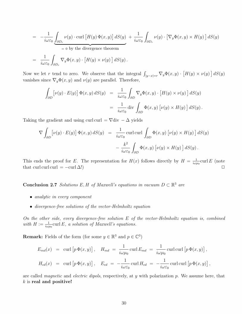
This ends the proof for E. The representation for H(x) follows directly by H = 1iωµ0
curlE (note
that curl curl curl = −curl ∆!) 2
Conclusion 2.7 Solutions E,H of Maxwell’s equations in vacuum D ⊂ R3 are
• analytic in every component
• divergence-free solutions of the vector-Helmholtz equation
On the other side, every divergence-free solution E of the vector-Helmholtz equation is, combinedwith H := 1
iωµ0curlE, a solution of Maxwell’s equations.
Remark: Fields of the form (for some y ∈ R3 and p ∈ C3)
Emd(x) = curl[pΦ(x, y)
], Hmd =
1
iωµ0
curlEmd =1
iωµ0
curl curl[pΦ(x, y)
],
Hed(x) = curl[pΦ(x, y)
], Eed = − 1
iωε0
curlHed = − 1
iωε0
curl curl[pΦ(x, y)
],
are called magnetic and electric dipols, respectively, at y with polarization p. We assume here, thatk is real and positive!
30
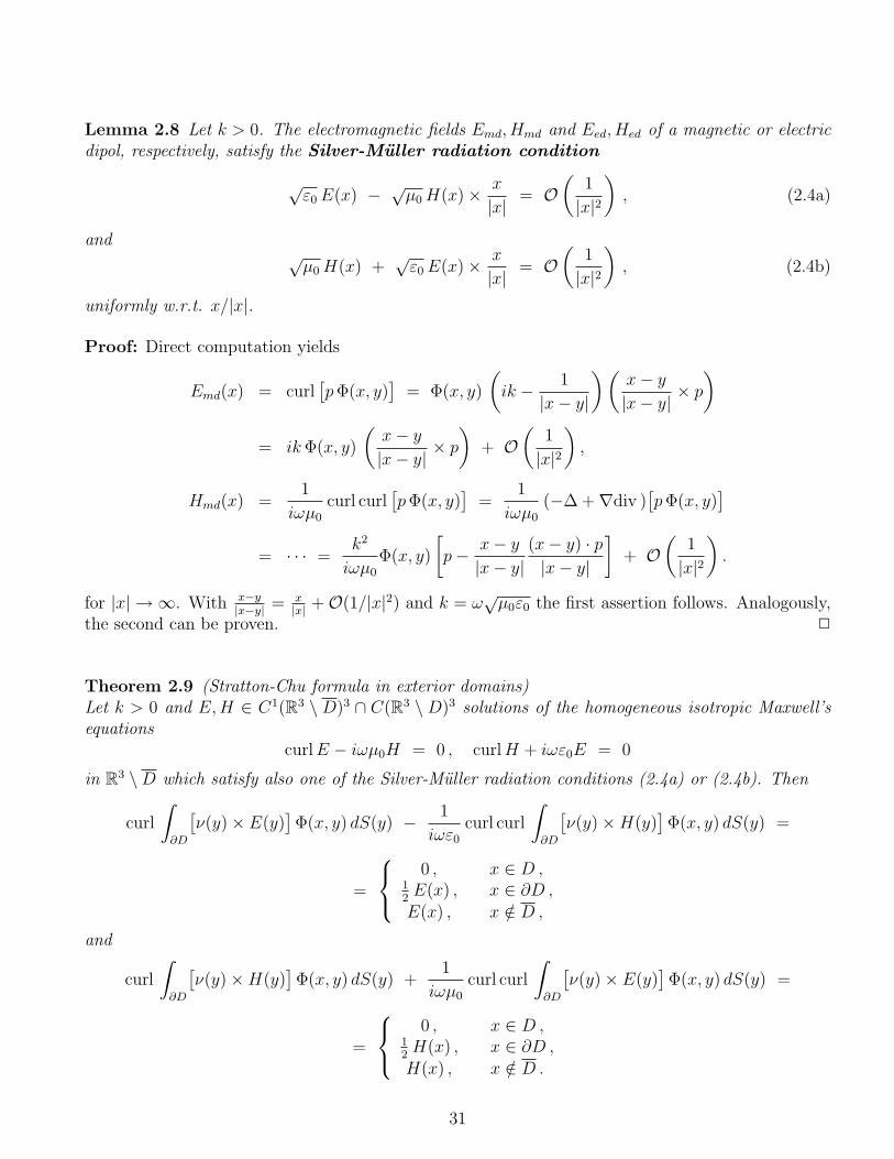
Lemma 2.8 Let k > 0. The electromagnetic fields Emd, Hmd and Eed, Hed of a magnetic or electricdipol, respectively, satisfy the Silver-Muller radiation condition
√ε0E(x) − √
µ0H(x)× x
|x|= O
(1
|x|2
), (2.4a)
andõ0H(x) +
√ε0E(x)× x
|x|= O
(1
|x|2
), (2.4b)
uniformly w.r.t. x/|x|.
Proof: Direct computation yields
Emd(x) = curl[pΦ(x, y)
]= Φ(x, y)
(ik − 1
|x− y|
) (x− y
|x− y|× p
)= ikΦ(x, y)
(x− y
|x− y|× p
)+ O
(1
|x|2
),
Hmd(x) =1
iωµ0
curl curl[pΦ(x, y)
]=
1
iωµ0
(−∆ +∇div )[pΦ(x, y)
]= · · · =
k2
iωµ0
Φ(x, y)
[p− x− y
|x− y|(x− y) · p|x− y|
]+ O
(1
|x|2
).
for |x| → ∞. With x−y|x−y| = x
|x| +O(1/|x|2) and k = ω√µ0ε0 the first assertion follows. Analogously,
the second can be proven. 2
Theorem 2.9 (Stratton-Chu formula in exterior domains)Let k > 0 and E,H ∈ C1(R3 \ D)3 ∩ C(R3 \ D)3 solutions of the homogeneous isotropic Maxwell’sequations
curlE − iωµ0H = 0 , curlH + iωε0E = 0
in R3 \D which satisfy also one of the Silver-Muller radiation conditions (2.4a) or (2.4b). Then
curl
∫∂D
[ν(y)× E(y)
]Φ(x, y) dS(y) − 1
iωε0
curl curl
∫∂D
[ν(y)×H(y)
]Φ(x, y) dS(y) =
=
0 , x ∈ D ,
12E(x) , x ∈ ∂D ,E(x) , x /∈ D ,
and
curl
∫∂D
[ν(y)×H(y)
]Φ(x, y) dS(y) +
1
iωµ0
curl curl
∫∂D
[ν(y)× E(y)
]Φ(x, y) dS(y) =
=
0 , x ∈ D ,
12H(x) , x ∈ ∂D ,H(x) , x /∈ D .
31

Proof: Let us first assume the radiation condition (2.4a). One applies Theorem 2.6 in the regionDR =
x /∈ D : |y| < R
for large values of R. Then the assertion follows if one can show that
IR := curl
∫|y|=R
[ν(y)× E(y)
]Φ(x, y) dS(y) − 1
iωε0
curl curl
∫|y|=R
[ν(y)×H(y)
]Φ(x, y) dS(y)
tends to zero as R → ∞. To do this we first prove that∫|y|=R
|E|2dS is bounded w.r.t. R. The
binomial theorem yields∫|y|=R
|√ε0E −
√µ0H × ν|2dS = ε0
∫|y|=R
|E|2dS + µ0
∫|y|=R
|H × ν|2dS
−2√ε0µ0 Re
∫|y|=R
E · (H × ν) dS .
We have by the divergence theorem∫|y|=R
E · (H × ν) dS =
∫∂D
E · (H × ν) dS +
∫∫DR
div (E ×H) dV
=
∫∂D
E · (H × ν) dS +
∫∫DR
[H) · curlE − E · curlH
]dV
=
∫∂D
E · (H × ν) dS +
∫∫DR
[iωµ0|H|2 − iωε0|E|2
]dV .
This term is purely imaginary, thus∫|y|=R
|√ε0E −
√µ0H × ν|2dS = ε0
∫|y|=R
|E|2dS + µ0
∫|y|=R
|H × ν|2dS
− 2√ε0µ0 Re
∫∂D
E · (H × ν) dS .
From this the boundedness of∫|y|=R
|E|2dS follows since the left hand side tends to zero by the
radiation condition (2.4a).Now we write IR in the form
IR = curl
∫|y|=R
[ν(y)× E(y)
]Φ(x, y) +
1
ikE(y)×∇yΦ(x, y)
dS(y)
− 1
iωε0
curl
∫|y|=R
([ν(y)×H(y)
]+
√ε0
µ0
E(y)
)×∇yΦ(x, y) dS(y) .
Let us first consider the second term. The bracket (· · · ) tends to zero as 1/R2 by the radiationcondition (2.4a). Taking the curl of the integral results in second order differentiations of Φ. SinceΦ and all derivatives decay as 1/R the total integrand decays as 1/R3. Therefore, this second termtends to zero because the surface area is only 4πR2.For the first term we observe that[
ν(y)× E(y)]Φ(x, y) +
1
ikE(y)×∇yΦ(x, y)
= E(y)×[− y
RΦ(x, y) +
1
ik
y − x
|y − x|Φ(x, y)
(ik − 1
|y − x|
)].
32

For fixed x and arbitrary y with |y| = R the bracket [· · · ] tends to zero of order 1/R2. The sameholds true for all of the partial derivatives w.r.t. x. Therefore, the first term can be estimated bythe inequality of Cauchy-Schwartz
c
R2
∫|y|=R
∣∣E(y)∣∣ dS ≤ c
R2
√∫|y|=R
12 dS
√∫|y|=R
∣∣E(y)∣∣2 dS =
c√
4π
R
√∫|y|=R
∣∣E(y)∣∣2 dS
and this tends also to zero.This proves the representation of E by using the first radiation condition (2.4a). The representationof H(x) follows again by computing H = 1
iωµ0curlE. If the second radiation condition (2.4b) is
assumned one can argue as before and derive the representation of H first. 2
Remarks:
• If E, H are solution of Maxwell’s equationen in vacuum R3 \ D then each of the radiationconditions implies the other one.
• The Silver-Muller radiation condition for solutions E, H of Maxwell’s equations is equivalentto the Sommerfeld radiation condition for every component of E and H.
• The representation theorem 2.9 and the Silver-Muller radiation condition imply the asymptoticbehaviour
E(x) = O(
1
|x|
)and H(x) = O
(1
|x|
)for |x| → ∞ uniformly w.r.t. all directions x/|x|.
2.2 Smoothness of Potentials
We have seen in the preceding section that any function can be represented by a combination ofvolume and surface potentials. The integral equation method for solving Maxwell’s equations relyheavily on the smoothness properties of these potentials.
2.2.1 The Scalar Volume and Surface Potentials
We recall the fundamental solution (in this subsection only for k ∈ R, k ≥ 0)
Φ(x, y) =eik|x−y|
4π|x− y|, x 6= y , (2.5)
and begin with the volume potential
w(x) =
∫∫D
ϕ(y) Φ(x, y) dV (y) , x ∈ R3 . (2.6)
33

Lemma 2.10 Let ϕ : D → C be piecewise continuous.3 Then w ∈ C1(R3) and
∂w
∂xj
(x) =
∫∫D
ϕ(y)∂Φ
∂xj
(x, y) dV (y) , x ∈ R3 , j = 1, 2, 3 . (2.7)
Proof: We fix j ∈ 1, 2, 3 and a real valued function η ∈ C1(R) with 0 ≤ η(t) ≤ 1 and η(t) = 0 fort ≤ 1 and η(t) = 1 for η ≥ 2. We set∫∫
D
ϕ(y)∂Φ
∂xj
(x, y) dV (y) , x ∈ R3 ,
and note that the integal exists as an improper integral by Lemma 2.2 since∣∣∣ ∂Φ∂xj
(x, y)∣∣∣ ≤ c
(|x−y|−2
)for some c > 0. Furthermore, set
wε(x) =
∫∫D
ϕ(y) Φ(x, y) η(|x− y|/ε
)dV (y) , x ∈ R3 .
Then wε ∈ C1(R3) and
v(x)− ∂wε
∂xj
(x) =
∫∫|y−x|≤2ε
ϕ(y)∂
∂xj
Φ(x, y)
[1− η
(|x− y|/ε
)]dV (y) ,
and thus ∣∣∣∣v(x)− ∂wε
∂xj
(x)
∣∣∣∣ ≤ ‖ϕ‖∞∫∫
|y−x|≤2ε
[∣∣∣∣ ∂Φ
∂xj
(x, y)
∣∣∣∣ +‖η′‖∞ε
∣∣Φ(x, y)∣∣] dV (y)
≤ c0
∫∫|y−x|≤2ε
[1
|x− y|2+
1
ε |x− y|
]dV (y)
= c0
2π∫0
π∫0
2ε∫0
[1
r2+
1
ε r
]r2 sin θ dr dθ dϕ = 16π c0 ε .
Therefore, ∂Wε/∂xj → v uniformly in R3. Thus w ∈ C1(R3) and ∂W/∂xj = v. 2
Theorem 2.11 Let ϕ : D → C be Holder-continuous, i.e. there exists α ∈ (0, 1] and c > 0with
∣∣ϕ(x) − ϕ(y)∣∣ ≤ c |x − y|α for all x, y ∈ D, and let w be the volume potential. Then w ∈
C2(D) ∩ C∞(R3 \D) and
∆w + k2w =
−ϕ , in D ,0 , in R3 \D .
Furthermore, if D0 is any C2−smooth domain with D ⊂ D0 then
∂2w
∂xi∂xj
(x) =
∫∫D0
∂2Φ
∂xi∂xj
(x, y)[ϕ(y)− ϕ(x)
]dV (y) − ϕ(x)
∫∂D0
∂Φ
∂xi
(x, y) νj(y) dS(y) (2.8)
for x ∈ D where we have extended ϕ by zero in D0 \D.
3This means: There exist finitely many domains Dj with D = ∪jDj such that ϕ|Djhas a continuous extension to
Dj for every j.
34

Proof: First we note that the volume integral in the last formula exists again by Lemma 2.2 since∣∣ϕ(y)− ϕ(x)∣∣∣∣∂2Φ/(∂xi∂xj)(x, y)
∣∣ ≤ c |x− y|α−3. The surface integral is no problem since x /∈ ∂D0.We fix i, j ∈ 1, 2, 3 and the same funtion η ∈ C1(R) as in the previous lemma. We definev := ∂w/∂xi and
u(x) :=
∫∫D0
∂2Φ
xixj
(x, y)[ϕ(y)− ϕ(x)
]dV (y) − ϕ(x)
∫∂D0
∂Φ
∂xi
(x, y) νj(y) dS(y)
vε(x) :=
∫∫D
ϕ(y) η(|x− y|/ε
) ∂Φ
∂xi
(x, y) dV (y) , x ∈ R3 .
Then vε ∈ C1(D) and for x ∈ D
∂vε
∂xj
(x) =
∫∫D
ϕ(y)∂
∂xj
η(|x− y|/ε
) ∂Φ
∂xi
(x, y)
dV (y)
=
∫∫D0
[ϕ(y)− ϕ(x)
] ∂
∂xj
η(|x− y|/ε
) ∂Φ
∂xi
(x, y)
dV (y)
+ ϕ(x)
∫∫D0
∂
∂xj
η(|x− y|/ε
) ∂Φ
∂xi
(x, y)
dV (y)
=
∫∫D0
[ϕ(y)− ϕ(x)
] ∂
∂xj
η(|x− y|/ε
) ∂Φ
∂xi
(x, y)
dV (y)
− ϕ(x)
∫∂D0
∂Φ
∂xi
(x, y) νj(y) dS(y)
provided 2ε ≤ d(x, ∂D0). In the last step we used the Divergence Theorem! Therefore,∣∣∣∣u(x)− ∂vε
∂xj
(x)
∣∣∣∣ ≤∫∫
|y−x|≤2ε
∣∣ϕ(y)− ϕ(x)∣∣ ∣∣∣∣ ∂
∂xj
(1− η
(|x− y|/ε
)) ∂Φ
∂xi
(x, y)
∣∣∣∣ dV (y)
≤ c
∫∫|y−x|≤2ε
(1
|y − x|3+
‖η′‖∞ε |y − x|2
)|y − x|α dV (y)
=
2ε∫0
(1
r1−α+‖η′‖∞ε
rα
)dr
≤ 4π c
[(2ε)α
α+
(2ε)1+α
(1 + α) ε
]≤ c ε ,
thus ∂vε/∂xj(x) → u(x) provided 2ε ≤ dist(x, ∂D). Therefore, ∂vε/∂xj → u uniformly on compactsubsets of D. Also, vε → v uniformly on compact subsets of D and thus w ∈ C2(D) and u =
35

∂2w/(∂xi∂xj). This proves (2.8). Finally, setting D0 = K(x,R):
∆w(x) = −k2
∫∫K(x,R)
Φ(x, y)[ϕ(y)− ϕ(x)
]dV (y)
− f(x)3∑
j=1
yj − xj
R
[exp(ikR)
4π R
(ik − 1/R
) xj − yj
R
]4π R2
= −k2w(x) + k2f(x)
∫∫K(x,R)
exp(ik|x− y|
)4π |x− y|
dV (y) − f(x) eikR(1− ikR) ,
i.e.
∆w(x) + k2w(x) = −f(x)
[eikR(1− ikR)− k2
∫∫K(x,R)
exp(ik|x− y|
)4π |x− y|
dV (y)
]︸ ︷︷ ︸
= 1
since
k2
∫∫K(x,R)
exp(ik|x− y|
)4π |x− y|
dV (y) = 4π k2
R∫0
exp(ikr)
4π rr2dr = k2
R∫0
r eikrdr
= · · · = −ikR eikR + eikR − 1 .
2
For any set T and α ∈ (0, 1] we define the space Cα(T ) of bounded Holder-continuous functionsv : T → C by
Cα(T ) :=
v ∈ C(T ) : v bounded and sup
x,y∈T, x6=y
∣∣v(x)− v(y)∣∣
|x− y|α< ∞
Note that any Holder-continuous function is uniformly continuous and, therefore, has a continuousextension to T . The space Cα(T ) is a normed space with norm
‖v‖Cα(T ) := supx∈T
∣∣v(x)∣∣︸ ︷︷ ︸= ‖v‖∞
+ supx,y∈T, x6=y
∣∣v(x)− v(y)∣∣
|x− y|α. (2.9)
Corollary 2.12 Let D be C2−smooth and T ⊂ R3 be a closed set with T ⊂ D or T ⊂ R3 \D. Thenthere exists c > 0 with
‖w‖C1(R3) ≤ c ‖ϕ‖∞ and ‖w‖C2(T ) ≤ c ‖ϕ‖Cα(D) (2.10)
for all ϕ ∈ Cα(∂D).
36

Proof: We estimate ∣∣Φ(x, y)∣∣ =
1
4π|x− y|,∣∣∣∣ ∂Φ
∂xj
(x, y)
∣∣∣∣ ≤ c1
[1
|x− y|2+
1
|x− y|
],∣∣∣∣ ∂2Φ
∂xi∂xj
(x, y)
∣∣∣∣ ≤ c2
[1
|x− y|3+
1
|x− y|2+
1
|x− y|
].
For x ∈ R3 we estimate, using (2.7) and Lemma 2.2 above,∣∣w(x)∣∣ ≤ ‖ϕ‖∞
∫∫D
1
4π|x− y|dV (y) ≤ c ‖ϕ‖∞ ,∣∣∣∣ ∂w∂xj
(x)
∣∣∣∣ ≤ ‖ϕ‖∞∫∫
D
∣∣∣∣ ∂Φ
∂xj
(x, y)
∣∣∣∣ dV (y) ≤ c ‖ϕ‖∞ ,
where the constant is independent of x and ϕ. This proves already the first estimate of (2.10). Letnow x ∈ T . If T ⊂ D then there exists δ > 0 with |x − y| ≥ δ for all x ∈ T and y ∈ ∂D. By (2.8)for D = D0 we have∣∣∣∣ ∂2w
∂xi∂xj
(x)
∣∣∣∣ ≤ ‖ϕ‖Cα(D)
∫∫D
∣∣∣∣ ∂2Φ
∂xi∂xj
(x, y)
∣∣∣∣ |x− y|α dV (y) + ‖ϕ‖∞∫
∂D
∣∣∣∣ ∂Φ
∂xi
(x, y)
∣∣∣∣ dS(y)
≤ c3 ‖ϕ‖Cα(D)
∫∫D
dV (y)
|x− y|3−α+ c4 ‖ϕ‖∞
∫∂D
dS(y)
|x− y|2
≤ c5 ‖ϕ‖Cα(D) +c4δ2‖ϕ‖∞
∫∂D
dS
≤ c‖ϕ‖Cα(D) .
If T ⊂ R3 \D then there exists δ > 0 with |x − y| ≥ δ for all x ∈ T and y ∈ D. Therefore, we canestimate ∣∣∣∣ ∂2w
∂xi∂xj
(x)
∣∣∣∣ ≤ ‖ϕ‖∞∫∫
D
∣∣∣∣ ∂2Φ
∂xi∂xj
(x, y)
∣∣∣∣ dV (y) ≤ ‖ϕ‖∞c
δ3
∫∫D
dV .
2
We continue with the single layer surface potential
v(x) =
∫∂D
ϕ(y) Φ(x, y) dS(y) , x ∈ R3 . (2.11)
First we note that for continuous densities ϕ the integral exists (as an improper integral) even forx ∈ ∂D since Φ has a singularity of the form
∣∣Φ(x, y)∣∣ = 1/(4π|x− y|). This follows from Lemma 2.2
above. Before we prove continuity of v we make the following general remark.
37

Remark 2.13 A function v : R3 → C is Holder continuous if
(a) v is bounded,
(b) v is Holder continuous in some Hρ,
(c) v is Lipschitz continuous in R3 \ Uδ for every δ > 0.
Again, Uρ is the strip around ∂D of thickness ρ and Uδ is the neighborhood of ∂D with thickness δ.
Proof : Choose δ > 0 such that U3δ ⊂ Hρ.Ist case: |x1−x2| < δ and x1 ∈ U2δ. Then x1, x2 ∈ U3δ ⊂ Hρ and Holder continuity follows from (b).2nd case: |x1 − x2| < δ and x1 /∈ U2δ. Then x1, x2 /∈ Uδ and thus from (c):∣∣v(x1)− v(x2)
∣∣ ≤ c|x1 − x2| ≤ cδ1−α|x1 − x2|α .
3rd case: |x1 − x2| ≥ δ. Then, by (a),
∣∣v(x1)− v(x2)∣∣ ≤ 2‖v‖∞ ≤ 2‖v‖∞
δα|x1 − x2|α .
Theorem 2.14 The single-layer potential v from (2.11) with continuous density ϕ is uniformlyHolder continuous in all of R3, and for every α ∈ (0, 1) there exists c > 0 (independent of ϕ) with
‖v‖Cα(R3) ≤ c‖ϕ‖∞ . (2.12)
Proof: We check the conditions (a), (b), (c) of the remark. Boundedness follows from Lemma 2.2since
∣∣Φ(x, y)∣∣ = 1/(4π|x− y|). For (b) and (c) we write
∣∣v(x1)− v(x2)∣∣ ≤ ‖ϕ‖∞
∫∂D
∣∣Φ(x1, y)− Φ(x2, y)∣∣ dS(y) (2.13)
and estimate∣∣Φ(x1, y)− Φ(x2, y)∣∣ ≤ 1
4π
∣∣∣∣ 1
|x1 − y|− 1
|x2 − y|
∣∣∣∣ +1
4π|x1 − y|∣∣eik|x1−y| − eik|x1−y|∣∣
≤ |x1 − x2|4π |x1 − y||x2 − y|
+k |x1 − x2|4π |x1 − y|
since∣∣exp(it)− exp(is)
∣∣ ≤ |t− s| for all t, s ∈ R.Now (c) follows since |xj − y| ≥ δ for xj /∈ Uδ.
To show (b), i.e. Holder continuity in Hρ0 let x1, x2 ∈ Hρ0 , we set Γz,r =y ∈ ∂D : |y− z| < r
and
split the domain of integration into Γz1,r and ∂D \ Γz1,r where we set r = 3|x1 − x2|. The integral
38

over Γz1,r is simply estimated by∫Γz1,r
∣∣Φ(x1, y)− Φ(x2, y)∣∣ dS(y) ≤ 1
4π
∫Γz1,r
dS(y)
|x1 − y|+
1
4π
∫Γz1,r
dS(y)
|x2 − y|
≤ 1
2π
∫Γz1,r
dS(y)
|z1 − y|+
1
2π
∫Γz2,2r
dS(y)
|z2 − y|
where we used |zj−y| ≤ 2|xj−y| for j = 1, 2 and Γz1,r ⊂ Γz2,2r because |y−z2| ≤ |y−z1|+ |z1−z2| ≤|y − z1|+ 2|x1 − x2| ≤ |y − z1|+ r. Using a local parametrization y = Ψ(v) for v ∈ K2(0, 1) one caneasily derive an estimate of the form4 ∫
Γz,r
dS(y)
|z − y|≤ c r
where c is independent of z. Therefore, we have shown that∫Γz1,r
∣∣Φ(x1, y)− Φ(x2, y)∣∣ dS(y) ≤ c
πr =
3c
π|x1 − x2| ≤ c |x1 − x2|α
where c is independent of xj.Now we continue with the integral over ∂D \ Γz1,r. We estimateFor y ∈ ∂D \Γz1,r we have 3|x1−x2| = r ≤ |y− z1| ≤ 2|y−x1|, thus |x2− y| ≥ |x1− y| − |x1−x2| ≥(1− 2/3) |x1 − y| = |x1 − y|/3 and therefore∣∣Φ(x1, y)− Φ(x2, y)
∣∣ ≤ 3|x1 − x2|4π |x1 − y|2
+k |x1 − x2|4π |x1 − y|
≤ 3|x1 − x2|π |z1 − y|2
+k |x1 − x2|2π |z1 − y|
since |z1 − y| ≤ 2|x1 − y|. Then we estimate∫∂D\Γz1,r
∣∣Φ(x1, y)− Φ(x2, y)∣∣ dS(y) ≤ |x1 − x2|
π
∫∂D\Γz1,r
[3
|z1 − y|2+
k
2|z1 − y|
]dS(y)
=|x1 − x2|α
π
∫∂D\Γz1,r
(r/3)1−α
[3
|z1 − y|2+
k
2|z1 − y|
]dS(y)
≤ |x1 − x2|α
π 31−α
∫∂D\Γz1,r
[3
|z1 − y|2−(1−α)+
k
2 |z1 − y|1−(1−α)
]dS(y)
since r1−α ≤ |y − z1|1−α for y ∈ ∂D \ Γz1,r. Therefore,∫∂D\Γz1,r
∣∣Φ(x1, y)− Φ(x2, y)∣∣ dS(y) ≤ 1
π 31−α|x1 − x2|α
[3 c1−α +
k
2c2−α
]4Here and in the following the constant c changes from line to line.
39

with the constants cβ from Lemma 2.2, part (b). Altogether we have shown the existence of c > 0with ∣∣v(x1)− v(x2)
∣∣ ≤ c ‖ϕ‖∞ |x1 − x2|α for all x1, x2 ∈ Hρ0
which ends the proof. 2
Before we continue with the investigation of the double layer surface potential we prove an auxiliaryresult which we will use often in the following.
Lemma 2.15 For ϕ ∈ Cα(∂D) and a ∈ C(∂D)3 define
w(x) =
∫∂D
[ϕ(y)− ϕ(z)
]a(y) · ∇yΦ(x, y) dS(y) , x ∈ Hρ0 ,
where x = z + tν(z) ∈ Hρ0 with |t| < ρ0 and z ∈ ∂D. Then the integral exists for x ∈ ∂D as animproper integral and w is Holder continuous in Hρ0 for any exponent β < α. Furthermore, thereexists c > 0 with
∣∣w(x)∣∣ ≤ c‖v‖Cβ(∂D) for all x ∈ Hρ0.
Proof: For x` = z` + t`ν(z`) ∈ Hρ0 , ` = 1, 2, we have to estimate
w(x1)− w(x2) =
∫∂D
[ϕ(y)− ϕ(z1)
]a(y) · ∇yΦ(x1, y)−
[ϕ(y)− ϕ(z2)
]a(y) · ∇yΦ(x2, y) dS(y) (2.14)
=[ϕ(z2)− ϕ(z1)
] ∫∂D
a(y) · ∇yΦ(x1, y) dS(y) +
+
∫∂D
[ϕ(y)− ϕ(z2)
]a(y) ·
[∇yΦ(x1, y)−∇yΦ(x2, y)
]dS(y)
and thus ∣∣w(x1)− w(x2)∣∣ ≤
∣∣ϕ(z2)− ϕ(z1)∣∣ ∣∣∣∣∫
∂D
a(y) · ∇yΦ(x1, y) dS(y)
∣∣∣∣ +
+ ‖a‖∞∫
∂D
∣∣ϕ(y)− ϕ(z2)∣∣ ∣∣∇yΦ(x1, y)−∇yΦ(x2, y)
∣∣ dS(y) (2.15)
We need the following estimates of Φ and its derivatives: There exists c > 0 with∣∣∇yΦ(x, y)∣∣ ≤ c
|x− y|2, x ∈ Hρ0 , y ∈ ∂D ,
∣∣∇yΦ(x1, y)−∇yΦ(x2, y)∣∣ ≤ c
|x1 − x2||x1 − y|3
, y ∈ ∂D , x` ∈ Hρ0 with |x1 − y| ≤ 3|x2 − y| .
Proof of these estimates: The first one is obvious. For the second one we observe that Φ(x, y) =φ(|x−y|) with φ(t) = exp(ikt)/(4πt), thus φ′(t) = φ(t)(ik−1/t) and φ′′(t) = φ′(t)(ik−1/t)+φ(t)/t2 =
40

φ(t)[(ik− 1/t)2 + 1/t2
]and therefore
∣∣φ′(t)∣∣ ≤ c1/t2 and
∣∣φ′′(t)∣∣ ≤ c2/t3 for 0 < t ≤ 1. For t ≤ 3s we
have∣∣φ′(t)− φ′(s)∣∣ =
∣∣∣∣∣∣t∫
s
φ′′(τ) dτ
∣∣∣∣∣∣ ≤ c2
∣∣∣∣∣∣t∫
s
dτ
τ 3
∣∣∣∣∣∣ =c22|t−2 − s−2|
=c22
|t2 − s2|t2s2
≤ c22|t− s|
(1
ts2+
1
t2s
)≤ c2
2|t− s|
(9
t3+
3
t3
)= 6c2
|t− s|t3
.
Setting t = |x1 − y| and s = |x2 − y| and observing that |t− s| ≤ |x1 − x2| yields the estimate∣∣∇yΦ(x1, y)−∇yΦ(x2, y)∣∣ =
∣∣∣∣φ′(|x1 − y|) y − x1
|y − x1|− φ′(|x2 − y|) y − x2
|y − x2|
∣∣∣∣≤
∣∣φ′(|x1 − y|)− φ′(|x2 − y|)∣∣ +
∣∣φ′(|x2 − y|)∣∣ ∣∣∣∣ y − x1
|y − x1|− y − x2
|y − x2|
∣∣∣∣≤ 6c2
|x2 − x1||y − x1|3
+ 2∣∣φ′(|x2 − y|)
∣∣ |x2 − x1||y − x1|
≤ 6c2|x2 − x1||y − x1|3
+ 2c1|x2 − x1|
|y − x1||y − x2|2≤ (6c2 + 18c1)
|x2 − x1||y − x1|3
.
This yields the second estimate.
Now we split the region of integration again into Γz1,r and ∂D \Γz1,r with r = 3|x1−x2| where againΓz,r = y ∈ ∂D : |y − z| < r. The integral (in the form (2.14)) over Γz1,r is estimated by5∫
Γz1,r
∣∣[ϕ(y)− ϕ(z1)]a(y) · ∇yΦ(x1, y)−
[ϕ(y)− ϕ(z2)
]a(y) · ∇yΦ(x2, y)
∣∣ dS(y) (2.16)
≤ c
∫Γz1,r
[|y − z1|α
1
|y − x1|2+ |y − z2|α
1
|y − x2|2
]dS(y)
≤ c
∫Γz1,r
|y − z1|α1
|y − z1|2dS(y) + c
∫Γz2,2r
|y − z2|α1
|y − z2|2dS(y)
since Γz1,r ⊂ Γz2,2r and |x`− y| ≥ |z`− y|/2. Therefore, using local coordinates, this term behaves asrα = 3α|x1 − x2|α ≤ c|x1 − x2|β.We finally consider the integral over ∂D \ Γz1,r und use the form (2.15):
I :=∣∣ϕ(z2)− ϕ(z1)
∣∣ ∣∣∣∣∣∫
∂D\Γz1,r
a(y) · ∇yΦ(x1, y) dS(y)
∣∣∣∣∣ +
+ ‖a‖∞∫
∂D\Γz1,r
∣∣ϕ(y)− ϕ(z2)∣∣ ∣∣∇yΦ(x1, y)−∇yΦ(x2, y)
∣∣ dS(y)
≤ c
∫∂D\Γz1,r
[|z2 − z1|α
1
|x1 − y|2+ |y − z2|α
|x1 − x2||x1 − y|3
]dS(y)
5The constant c is different from line to line.
41

Since y ∈ ∂D \ Γz1,r we use the estimates
• |x1 − x2| = r3≤ 1
3|y − z1| ≤ 2
3|y − x1| < |y − x1| and
• |y − z2| ≤ 2|y − x2| ≤ 2|y − x1|+ 2|x1 − x2| ≤ 4|y − x1|,
thus
I ≤ c
∫∂D\Γz1,r
[|x2 − x1|α
1
|z1 − y|2+
|x1 − x2||x1 − y|3−α
]dS(y)
≤ c′|x1 − x2|β∫
∂D\Γz1,r
[|x2 − x1|α−β 1
|z1 − y|2+|x1 − x2|1−β
|z1 − y|3−α
]dS(y)
≤ c|x1 − x2|β∫
∂D\Γz1,r
1
|z1 − y|2−(α−β)dS(y) ≤ c cα−β|x1 − x2|β
with the constant cα−β from Lemma 2.2. This, together with (2.16) proves the Holder-continuity ofw. The proof of the estimate
∣∣w(x)∣∣ ≤ v‖ϕ‖Cβ(∂D) for x ∈ Hρ0 is simpler and left to the reader. 2
Now we continue with the double layer surface potential
v(x) =
∫∂D
ϕ(y)∂Φk
∂ν(y)(x, y) dS(y) , x ∈ R3 \ ∂D , (2.17)
for Holder-continuous densities ϕ. Here we indicate the dependence on k ≥ 0 by writing Φk.
Theorem 2.16 The double layer potential v from (2.17) with Holder-continuous density ϕ ∈ Cα(∂D)can be continuously extended from D to D and from R3 \D to R3 \D with limiting values
limx→x0, x∈D
v(x) = −1
2ϕ(x0) +
∫∂D
ϕ(y)∂Φk
∂ν(y)(x0, y) dS(y) , x0 ∈ ∂D , (2.18a)
limx→x0, x/∈D
v(x) = +1
2ϕ(x0) +
∫∂D
ϕ(y)∂Φk
∂ν(y)(x0, y) dS(y) , x0 ∈ ∂D . (2.18b)
v is Holder-continuous in D and in R3 \D with exponent β for every β < α. The integrals exist asimproper integrals.
Proof: First we note that the integrals exist since for x0, y ∈ ∂D we can estimate∣∣∣∣ ∂Φk
∂ν(y)(x0, y)
∣∣∣∣ =
∣∣∣∣exp(ik|x0 − y|)4π|x0 − y|
(ik − 1
|x0 − y|
)∣∣∣∣∣∣ν(y) · (y − x0)
∣∣|y − x0|
≤ c
|x0 − y|.
by Lemma 1.5. Furthermore, v has a decomposition into v = v0 + v1 where
v0(x) =
∫∂D
ϕ(y)∂Φ0
∂ν(y)(x, y) dS(y) , x ∈ R3 \ ∂D ,
v1(x) =
∫∂D
ϕ(y)∂(Φk − Φ0)
∂ν(y)(x, y) dS(y) , x ∈ R3 \ ∂D .
42

It is easily seen that the kernel K(x, y) = ϕ(y) ∂(Φk−Φ0)∂ν(y)
(x, y) of the integral in the definition of v1
is continuous in R3 × R3 and continuously differentiable with respect to x and bounded in the set(x, y) ∈ R3 × ∂D : x 6= y
. From this it follows that v1 is Holder-continuous in all of R3. Also this
is easy to prove.
We continue with the analysis of v0 and note that we have again prove estimates of the form (a) and(b) of Remark 2.13.First, for x ∈ Uδ/4 we have x = z + tν(z) with |t| < δ/4 and z ∈ ∂D. We write v0(x) in the form
v0(x) =
∫∂D
[ϕ(y)− ϕ(z)
] ∂Φ0
∂ν(y)(x, y) dS(y)︸ ︷︷ ︸
= v0(x)
+ ϕ(z)
∫∂D
∂Φ0
∂ν(y)(x, y) dS(y) .
The function v0 is Holder continuous in Uδ/4 with exponent β < α by Lemma 2.15 (take a(y) = ν(y)).This proves the estimate (a) and (b) of Remark 2.13 for v0.
Now we go back to the decomposition
v0(x) = v0(x) + ϕ(z)
∫∂D
∂Φ0
∂ν(y)(x, y) dS(y)
By Green’s representation (Theorem 2.3) for k = 0 and u = 1 we observe that∫∂D
∂Φ0
∂ν(y)(x, y) dS(y) =
−1 , x ∈ D ,−1/2 , x ∈ ∂D ,
0 , x /∈ D .
Therefore,
limx→x0, x∈D
v0(x) = v0(x0)− ϕ(x0) = v0(x0) +1
2ϕ(x0)− ϕ(x0) = −1
2ϕ(x0) ,
limx→x0, x/∈D
v0(x) = v0(x0) = v0(x0) +1
2ϕ(x0) .
This ends the proof. 2
In the following we write
v(x0)∣∣− = lim
x→x0, x∈Dv(x) and v(x0)
∣∣+
= limx→x0, x/∈D
v(x) and
∂v
∂ν(x0)
∣∣∣∣−
= limx→x0, x∈D
ν(x0) · ∇v(x) and∂v
∂ν(x0)
∣∣∣∣+
= limx→x0, x/∈D
ν(x0) · ∇v(x) .
Before we come to the derivative of the single layer potential we have to introduce two more notionsfrom differential geometry, the surface gradient and surface divergence.
Let Ψ : K2(0, 1) → U∩∂D be a parametrization of the part U∩∂D of the boundary. Then ∂Ψ(u)/∂uj,
j = 1, 2, span the tangent plane at x = Ψ(u). The Jacobian is Ψ′(u) =[
∂Ψ∂u1
(u) ∂Ψ∂u2
(u)]∈ R3×2. The
invertible (!) matrixG(u) = Ψ′(u)>Ψ′(u) ∈ R2×2
43

is called the first fundamental tensor of differential geometry. We set g(u) = detG(u). It is easy tosee that
P (u) = Ψ′(u)G−1(u) Ψ′(u)> ∈ R3×3
is the projection matrix onto the tangent plane at x = Ψ(u). Indeed, this follows from[P (u)− I
]>Ψ′(u) = Ψ′(u)G−1(u) Ψ′(u)>Ψ′(u)︸ ︷︷ ︸
= G(u)
− Ψ′(u) = 0 .
Let now f : U → C a function defined on the neighborhood U of ∂D. Define f : K2(0, 1) → C byf(u) = f
(Ψ(u)
), u ∈ K2(0, 1). Then ∇uf(u) = Ψ′(u)>∇xf(x)|x=Ψ(u) and its projection onto the
tangent plane is given by
P (u)∇xf(x)|x=Ψ(u) = Ψ′(u)G−1(u) Ψ′(u)>∇xf(x)|x=Ψ(u) = Ψ′(u)G−1(u)∇uf(u) , u ∈ K2(0, 1) .
The right hand side serves as the definition of the surface gradient also if the function f is definedonly on ∂D ∩ U .
Definition 2.17 Let Ψ : K2(0, 1) → U ∩ ∂D be a parametrization of the part U ∩ ∂D.
(a) For differentiable6 f : U ∩ ∂D → C we define the surface gradient by
Grad f(x) = Ψ′(u)G−1(u)∇u(f Ψ)(u)|u=Ψ−1(x) .
(b) For differentiable vector fields F : U ∩∂D → C3 which are tangential fields, i.e. ν(x) ·F (x) = 0for all x, we define the surfave divergence by
DivF (x) =1√g(u)
∂
∂u1
[√g(u) F1(u)
]+
∂
∂u2
[√g(u) F2(u)
].
Here, Fj denotes the component with respect to the basis∂Ψ(u)/∂u1, ∂Ψ(u)/∂u2
, i.e.
(F Ψ)(u) = F1(u)∂Ψ∂u1
(u) + F2(u)∂Ψ∂u2
(u) = Ψ′(u)F (u) with F (u) =(F1(u), F2(u)
)>.
For functions defined in a neighborhood of ∂D the surface gradient is just the orthogonal projectionof the ordinary gradient onto the tangential plane at x ∈ ∂D. From the definition it is clear that itis a tangential vector at x ∈ ∂D.
Example 2.18 Let D = K(0, 1) be the unit ball. We parametrize the boundary by spherical coordi-nates
Ψ(θ, φ) =(sin θ cosφ, sin θ sinφ, cos θ)> .
Then the surface gradient and surface divergence are given by
Grad f(θ, φ) =∂f
∂θ(θ, φ) θ +
1
sin θ
∂f
∂φ(θ, φ) φ ,
DivF (θ, φ) =1
sin θ
∂
∂θ
(sin θ Fθ(θ, φ)
)+
1
sin θ
∂Fφ
∂φ(θ, φ) ,
6i.e. f Ψj : K2(0, 1) → C is differentiable for every j
44

where θ = (cos θ cosφ, cos θ sinφ,− sin θ)> and φ = (− sin θ sinφ, sin θ cosφ, 0)> are the tangentialvectors which span the tangent plane and Fθ, Fφ are the components of F w.r.t. these vectors, i.e.
F = Fθθ + Fφφ. From this we note that
Div Grad f(θ, φ) =1
sin θ
∂
∂θ
(sin θ
∂f
∂θ(θ, φ)
)+
1
sin2 θ
∂2f
∂φ2(θ, φ) .
This differential operator is called the Laplace-Beltrami operator and is sometimes denotes by ∆S =Div Grad .
Theorem 2.19 Let F : ∂D → C3 be a continuously differentiable tangential field and f : ∂D → Ca continuously differentiable scalar function. Then∫
∂D
[f(x) DivF (x) + F (x) ·Grad f(x)
]dS = 0 .
Proof: Let ∂D ⊂⋃m
j=1 Uj and Ψj : K2(0, 1) → U ∩ ∂D be a local parametrization of the boundary.Let φj : j = 1, . . . ,m be a partition of unity corresponding to Uj : j = 1, . . . ,m, i.e.
• φj ∈ C∞(R3) with 0 ≤ φj ≤ 1 in R3,
• the support supp Ψj = closurex ∈ R : φj(x) 6= 0 is contained in Uj,
•∑m
j=1 φj(x) = 1 for all x ∈ ∂D.
Then we can write f =∑
j fj with fj(x) = φj(x)f(x) and compute∫∂D
[f(x) DivF (x) + F (x) ·Grad f(x)
]dS =
m∑j=1
∫∂D
[fj(x) DivF (x) + F (x) ·Grad fj(x)
]dS .
We note that (F Ψj)(u) = Ψ′j(u)F (u) on K2(0, 1) where F (u) :=
((F1 Ψ)(u), (F2 Ψ)(u)
)>.
Furthermore, the surface differential dS on Uj ∩ ∂D is given by
dS =
∣∣∣∣∂Ψj
∂u1
(u)× ∂Ψj
∂u2
(u)
∣∣∣∣ du =√gj(u) du .
45

Therefore, with (1.22c),
Ij :=
∫Uj∩∂D
[fj(x) DivF (x) + F (x) ·Grad fj(x)
]dS
=
∫K2(0,1)
[(fj Ψj)(u)
1√gj(u)
div[√
gj(u) F (u)]
+ (F Ψj)(u)>Ψ′
j(u)G−1j (u)∇(fj Ψj)(u)
]√gj(u) du
=
∫K2(0,1)
[(fj Ψj)(u) div
[√gj(u) F (u)
]+ (F Ψj)(u)
>Ψ′j(u)G
−1j (u)∇(fj Ψj)(u)
√gj(u)
]du
=
∫K2(0,1)
[−F (u)>∇(fj Ψj)(u) + (F Ψj)(u)
>Ψ′j(u)G
−1j (u)∇(fj Ψj)(u)
]√gj(u) du .
The bracket [· · · ] vanishes since (F Ψj)(u)>Ψ′
j(u)G−1j (u) = F (u)>Ψ′
j(u)>Ψ′
j(u)G−1j (u) = F (u)>. 2
Corollary 2.20 Let w ∈ C1(D)3 such that w, curlw ∈ C(D)3. Then the surface divergence of ν×wexists and is given by
Div (ν × w) = −ν · curlw on ∂D . (2.19)
Proof: Let ϕ ∈ C1(D) be arbitrary. By Gauss’ theorem:∫∂D
ϕν · curlw dS =
∫∫D
div (ϕ curlw) dV =
∫∫D
∇ϕ · curlw dV
=
∫∫D
div (w ×∇ϕ) dV =
∫∂D
ν · (w ×∇ϕ) dS
=
∫∂D
(ν × w) ·GradϕdS = −∫
∂D
Div (ν × w)ϕdS .
The assertion follows since ϕ is arbitrary. 2
Remark: This result has consequences for solutions (E,H) of Maxwell’s equations. If we requirecontinuity of the normal component ν ·E of E then this implies that the surface divergence Div (ν×H)of the tangential component of H exists and is continuous7.
Now we continue with the derivative of the single layer potential (2.11), i.e.
v(x) =
∫∂D
ϕ(y) Φ(x, y) dS(y) , x ∈ R3 .
7at least, if ε and σ are smooth
46

Theorem 2.21 The derivative of the single layer potential v from (2.11) with Holder-continuousdensity ϕ ∈ Cα(∂D) can be continuously extended from D to D and from R3 \ D to R3 \ D. Thetangential component is continuous, i.e. Grad v|− = Grad v|+, and the limiting values of the normalderivatives are
∂v
∂ν(x)
∣∣∣∣±
= ∓1
2ϕ(x) +
∫∂D
ϕ(y)∂Φ
∂ν(x)(x, y) dS(y) , x ∈ ∂D . (2.20)
The integral exists as an improper integral.
Proof: We note that the integral exists (see proof of Theorem 2.16). First we consider the density1, i.e. we set
v1(x) =
∫∂D
Φ(x, y) dS(y) , x ∈ R3 .
Let a ∈ R3 be any fixed vector. For x /∈ ∂D we compute, using the splitting of the gradient into thenormal and tangential components and equation (2.19)
a · ∇v1(x) =
∫∂D
a · ∇xΦ(x, y) dS(y) = −∫
∂D
a · ∇yΦ(x, y) dS(y)
= −∫
∂D
[a · ν(y)
] ∂Φ
∂ν(y)(x, y) dS(y) −
∫∂D
at(y) ·Grad yΦ(x, y) dS(y)
= −∫
∂D
[a · ν(y)
] ∂Φ
∂ν(y)(x, y) dS(y) +
∫∂D
Div at(y) Φ(x, y) dS(y)
where at(y) = ν(y)×(a×ν(y)
)is the tangential component of a. If we let a be one of the coordinate
unit vectors ej, j = 1, 2, 3, then
∇v1(x) = −∫
∂D
ν(y)∂Φ
∂ν(y)(x, y) dS(y) +
∫∂D
H(y) Φ(x, y) dS(y) , x /∈ ∂D , (2.21)
where H(y) =(Div e1t (y),Div e2t (y),Div e3t (y)
)> ∈ R3.
The right hand side is the sum of a double and a single layer potential. By Theorems 2.14 and 2.16it has a continuous extension to the boundary from the inside and the outside with limiting values
∇v1(x)|± = ∓1
2ν(x) −
∫∂D
ν(y)∂Φ
∂ν(y)(x, y) dS(y) +
∫∂D
H(y) Φ(x, y) dS(y) for x ∈ ∂D .
In particular, the tangential component is continuous and for the normal derivatives we have
∂v1
∂ν(x)
∣∣∣∣±
= ∓1
2+ ν(x) ·
∫∂D
[−ν(y) ∂Φ
∂ν(y)(x, y) dS(y) + H(y) Φ(x, y)
]dS(y) , x ∈ ∂D .
We compute the integral by the same arguments as before. Note, however, that now the integrand issingular at y = x. Therefore, choose any function ψ ∈ C∞(R) with ψ(t) = 0 for t ≤ 1/2 and ψ(t) = 1
47
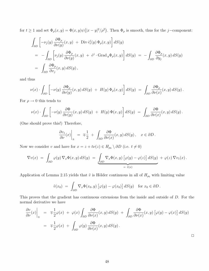
for t ≥ 1 and set Φρ(x, y) = Φ(x, y)ψ(|x− y|2/ρ2
). Then Φρ is smooth, thus for the j−component:∫
∂D
[−νj(y)
∂Φρ
∂ν(y)(x, y) + Div ej
t(y) Φρ(x, y)
]dS(y)
= −∫
∂D
[νj(y)
∂Φρ
∂ν(y)(x, y) + ej ·Grad yΦρ(x, y)
]dS(y) = −
∫∂D
∂Φρ
∂yj
(x, y) dS(y)
=
∫∂D
∂Φρ
∂xj
(x, y) dS(y) ,
and thus
ν(x) ·∫
∂D
[−ν(y) ∂Φρ
∂ν(y)(x, y) dS(y) + H(y) Φρ(x, y)
]dS(y) =
∫∂D
∂Φρ
∂ν(x)(x, y) dS(y) .
For ρ→ 0 this tends to
ν(x) ·∫
∂D
[−ν(y) ∂Φ
∂ν(y)(x, y) dS(y) + H(y) Φ(x, y)
]dS(y) =
∫∂D
∂Φ
∂ν(x)(x, y) dS(y) .
(One should prove this!) Therefore,
∂v1
∂ν(x)
∣∣∣∣±
= ∓1
2+
∫∂D
∂Φ
∂ν(x)(x, y) dS(y) , x ∈ ∂D .
Now we consider v and have for x = z + tν(z) ∈ Hρ0 \ ∂D (i.e. t 6= 0)
∇v(x) =
∫∂D
ϕ(y)∇xΦ(x, y) dS(y) =
∫∂D
∇xΦ(x, y)[ϕ(y)− ϕ(z)
]dS(y)︸ ︷︷ ︸
= v(x)
+ ϕ(z)∇v1(x) .
Application of Lemma 2.15 yields that v is Holder continuous in all of Hρ0 with limiting value
v(x0) =
∫∂D
∇xΦ(x0, y)[ϕ(y)− ϕ(x0)
]dS(y) for x0 ∈ ∂D .
This proves that the gradient has continuous extensions from the inside and outside of D. For thenormal derivative we have
∂v
∂ν(x)
∣∣∣∣±
= ∓1
2ϕ(x) + ϕ(x)
∫∂D
∂Φ
∂ν(x)(x, y) dS(y) +
∫∂D
∂Φ
∂ν(x)(x, y)
[ϕ(y)− ϕ(x)
]dS(y)
= ∓1
2ϕ(x) +
∫∂D
ϕ(y)∂Φ
∂ν(x)(x, y) dS(y) .
2
48
2.2.2 Vector Potentials
We continue with the vector potentials. Motivated by the Stratton-Chu formulas we have toconsider the curl and the double-curl of the single layer potential
v(x) =
∫∂D
a(y) Φ(x, y) dS(y) , x ∈ R3 , (2.22)
where a ∈ Cα(∂D)3 is a tangential field, i.e. a(y) · ν(y) = 0 for all y ∈ ∂D.
Theorem 2.22 The curl of the potential v from (2.22) with Holder continuous tangential field a ∈Cα(∂D)3 can be continuously extended from D to D and from R3 \D to R3 \D. The limiting valuesof the tangential components are
ν(x)× curl v(x)∣∣± = ±1
2a(x) + ν(x)×
∫∂D
curl x
[a(y)Φ(x, y)
]dS(y) , x ∈ ∂D . (2.23)
The integral exists as an improper integral.If, in addition, the surface divergence Div a is continuous, then div v is continuous in all of R3.If, furthermore, Div a ∈ Cα(∂D) then curl curl v can be continuously extended from D to D and fromR3 \D to R3 \D. The limiting values are
div v(x)∣∣± =
∫∂D
Φ(x, y) Div a(y) dS(y) , x ∈ ∂D ,
ν × curl curl v∣∣+
= ν × curl curl v∣∣− on ∂D ,
ν(x) · curl curl v(x)∣∣± = ∓1
2Div a(x)
+
∫∂D
[Div a(y)
∂Φ
∂ν(x)(x, y) + k2ν(x) · a(y) Φ(x, y)
]dS(y) , x ∈ ∂D .
Proof: We can write the second term on the right hand side of (2.23) in the form
ν(x)×∫
∂D
curl x
[a(y)Φ(x, y)
]dS(y) =
∫∂D
ν(x)×[∇xΦ(x, y)× a(y)
]dS(y)
=
∫∂D
[ν(x)− ν(y)
]×
[∇xΦ(x, y)× a(y)
]+
∂Φ
∂ν(y)(x, y) a(y)
dS(y)
and the integrand is weakly singular.
The components of curl v are combinations of partial derivatives of the single layer potential. There-fore, by Theorem 2.21 the field curl v has continuous extensions to ∂D from both sides. It remainsto show the representation of the tangential components of these extensions on the boundary. We
49

write x = z + tν(z), z ∈ ∂D, 0 < |t| < ρ0, and have
ν(z)× curl v(x) =
∫∂D
ν(z)×[∇xΦ(x, y)× a(y)
]dS(y)
=
∫∂D
[ν(z)− ν(y)
]×
[∇xΦ(x, y)× a(y)
]dS(y) +
∫∂D
a(y)∂Φ
∂ν(y)(x, y) dS(y) .
The first term is continuous in all of R3 by Lemma 2.15, the second in R3 \∂D because it is a doublelayer potential. The limiting values are
ν(x)× curl v(x)∣∣± =
∫∂D
[ν(x)− ν(y)
]×
[∇xΦ(x, y)× a(y)
]dS(y)
±1
2a(x) +
∫∂D
a(y)∂Φ
∂ν(y)(x, y) dS(y)
= ±1
2a(x) +
∫∂D
ν(x)×[∇xΦ(x, y)× a(y)
]dS(y)
which has the desired form. For the divergence we write
div v(x) =
∫∂D
a(y) · ∇xΦ(x, y) dS(y) = −∫
∂D
a(y) · ∇yΦ(x, y) dS(y)
= −∫
∂D
a(y) ·Grad yΦ(x, y) dS(y) =
∫∂D
Φ(x, y) Div a(y) dS(y)
and this is a single layer potential and thus continuous. Finally, since curl curl = ∇div − ∆ and∆xΦ(x, y) = −k2Φ(x, y),
curl curl v(x) = ∇div
∫∂D
a(y) Φ(x, y) dS(y) + k2
∫∂D
a(y) Φ(x, y) dS(y)
= ∇∫
∂D
Φ(x, y) Div a(y) dS(y) + k2
∫∂D
a(y) Φ(x, y) dS(y)
from which the assertion follows by Theorem 2.21. 2
50

3 Electromagnetic Scattering From a Perfect Conductor
3.1 Formulation of the Problem and Uniqueness
For this chapter we make the following assumptions on the data:
Assumption: Let the wave number be given by k = ω√ε0µ0 > 0 with constants ε0, µ0 > 0. Let
D ⊂ R3 be bounded and C2−smooth such that the complement R3 \D is connected.
Scattering Problem: Given a solution (Ei, H i) of the Maxwell system
curlEi − iωµ0Hi = 0 , curlH i + iωε0E
i = 0 in some neighborhood of D ,
determine the total fields E,H ∈ C1(R3 \D) ∩ C(R3 \D) such that
curlE − iωµ0H = 0 and curlH + iωε0E = 0 in R3 \D ,
E satisfies the boundary conditionν × E = 0 on ∂D , (3.1)
and the radiating parts Es = E−Ei and Hs = H−H i satisfy the Silver Muller radiation conditions
√ε0E
s(x) − √µ0H
s(x)× x
|x|= O
(1
|x|2
), (3.2a)
andõ0H
s(x) +√ε0E
s(x)× x
|x|= O
(1
|x|2
), (3.2b)
uniformly w.r.t. x/|x|. Clearly, after renaming the unknown fields, this is a special case of thefollowing problem:
Exterior Boundary Value Problem: Given a tangential field8 c ∈ Cα(∂D)3 such that Div c ∈Cα(∂D) determine radiating9 solutions Es, Hs ∈ C1(R3 \D) ∩ C(R3 \D) of
curlEs − iωµ0Hs = 0 and curlHs + iωε0E
s = 0 in R3 \D , (3.3a)
such that Es satisfies the boundary condition
ν × Es = c on ∂D . (3.3b)
We note again that the assumption on the surface divergence of c is necessary by Corollary 2.20.
First we want to prove that there exists at most one solution of this boundary value problem andtherefore also to the scattering problem.
The following Lemma is fundamental and tells us, that a solution of the Helmholtz equation ∆u +k2u = 0 for real and positive (!) k cannot decay faster than 1/|x| as x tends to infinity.
8i.e. ν(x) · c(x) = 0 on ∂D9i.e. Es, Hs satisfy the radiating conditions (3.2a) and (3.2b)
51

Lemma 3.1 (Rellich’s Lemma) Under the above assumption on D let u ∈ C2(R3 \D) be a solutionof the Helmholtz equation ∆u+ k2u = 0 in R3 \D such that
limR→∞
∫|x|=R
|u|2 dS = 0 and limR→∞
∫|x|=R
∣∣∣∣ x|x| · ∇u(x)∣∣∣∣2 dS = 0 .
Then u vanishes in R3 \D.
Proof:10 The proof is lengthy, and we will structure it. First we choose R0 > 0 such that D ⊂K(0, R0). We can assume that u is real valued (take real- and imaginary parts separately).
1st step: Transforming the integral onto the unit sphere S2 = x ∈ R3 : |x| = 1 we conclude that∫|x|=R
∣∣u(x)∣∣2 dS(x) =
∫|x|=1
∣∣u(rx)|2 r2 dS(x) and
∫|x|=R
∣∣∣∣∂u∂r (rx)
∣∣∣∣2 r2 dS(x) (3.4)
tend to zero as r tends to infinity. We transform the partial differential equation into an ordinarydifferential equation (not quite!) for the function v(r, θ, φ) = r u(r, θ, φ) w.r.t. r. We write v(r)and v′(r) and v′′(r) for v(r, ·.·) and ∂v(r, ·, ·)/∂r and ∂2v(r, ·, ·)/∂r2, respectively. Then (3.4) yieldsthat ‖v(r)‖L2(S2) → 0 and ‖v′(r)‖L2(S2) → 0 as r → ∞. The latter follows from ∂
∂r
(ru(r, ·, ·)
)=
1r
(ru(r, ·, ·)
)+ r ∂u
∂r(r, ·, ·) and the triangle inequality.
We observe that Reu = 1rv, thus r2 ∂Re u
∂r= −v + r ∂v
∂rand ∂
∂r
(r2 ∂Re u
∂r
)= r ∂2v
r2 , thus
0 =1
r2
∂
∂r
(r2∂Reu
∂r(r, θ, φ)
)+
1
r2∆SReu(r, θ, φ) + k2Reu(r, θ, φ)
=1
r
[∂2v
∂r2(r, θ, φ) + k2v(r, θ, φ) +
1
r2∆Sv(r, θ, φ)
],
i.e.
v′′(r) + k2v(r) +1
r2∆Sv(r) = 0 for r ≥ R0 , (3.5)
where again ∆S = Div Grad denotes the Laplace-Beltrami operator, i.e.
(∆Sw)(θ, φ) =1
sin θ
∂
∂θ
(sin θ
∂w
∂θ(θ, φ)
)+
1
sin2 θ
∂2w
∂φ2(θ, φ)
for any w ∈ C2(S2). It is easily seen either by direct integration or by application of Theorem 2.19that ∆S is selfadjoint and negative definite, i.e.(
∆Sv, w)
L2(S2)=
(v,∆Sw
)L2(S2)
and(∆Sv, v
)L2(S2)
≤ 0 for all v, w ∈ C2(S2) .
2nd step: We introduce the functions E, vm and F by
E(r) := ‖v′(r)‖2L2(S2) + k2‖v(r)‖2
L2(S2) +1
r2
(∆Sv(r), v(r)
)L2(S2)
, r ≥ R0 ,
vm(r) := rmv(r) , r ≥ R0 , m ∈ N ,
F (r,m, c) := ‖v′m(r)‖2L2(S2) +
(k2 +
m(m+ 1)
r2− 2c
r
)‖vm(r)‖2
L2(S2) +1
r2
(∆Svm(r), vm(r)
)L2(S2)
,
10We took the proof from the monograph Partielle Differentialgleichungen zweiter Ordnung by R. Leis
52
for r ≥ R0, m ∈ N, c ≥ 0. In the following we write ‖ · ‖ and (·, ·) for ‖ · ‖L2(S2) and (·, ·)L2(S2),respectively. We show:
(a) E satisfies E ′(r) ≥ 0 for all r ≥ R0.
(b) The functions vm solve the differential equation
v′′m(r) − 2m
rv′m(r) +
(m(m+ 1)
r2+ k2
)vm(r) +
1
r2∆Svm(r) = 0 . (3.6)
(c) For every c > 0 there exist r0 = r0(c) ≥ R0 and m0 = m0(c) ∈ N such that
∂
∂r
[r2F (r,m, c)
]≥ 0 for all r ≥ r0, m ≥ m0 .
(d) Expressed in terms of v the function F has the forms
F (r,m, c) = r2m
∥∥∥v′(r) +m
rv(r)
∥∥∥2
+
(k2 +
m(m+ 1)
r2− 2c
r
)‖v(r)‖2
+1
r2
(∆Sv(r), v(r)
)(3.7a)
= r2m
E(r) +
2m
r
(v(r), v′(r)
)+
(m(2m+ 1)
r2− 2c
r
)‖v(r)‖2
. (3.7b)
Proof of these statements:(a) We just differentiate E and substitute the second derivative from (3.5). Note that d
dr‖v(r)‖2 =
2(v, v′) and ddr
(∆Sv, v
)= 2
(∆Sv, v
′):E ′(r) = 2
(v′(r), v′′(r)
)+ 2k2
(v(r), v′(r)
)− 1
r3
(∆Sv(r), v(r)
)+
2
r2
(∆Sv(r), v
′(r))
= 2
(v′(r) ,
[v′′(r) + k2v(r) +
1
r2∆Sv(r)
])− 1
r3
(∆Sv(r), v(r)
)= − 1
r3
(∆Sv(r), v(r)
)≥ 0 .
(b) We substitute v(r) = r−mvm(r) into (3.5) and obtain directly (3.6). We omit the calculation.
(c) Again we differentiate r2F (r,m, c) w.r.t. r, substitute the form of v′′m from (3.6) and obtain
∂
∂r
[r2F (r,m, c)
]= 2r‖v′m(r)‖2 + 2r2
(v′m(r), v′′m(r)
)+ 2(k2r − c)‖vm(r)‖2
+ 2r2
(k2 +
m(m+ 1)
r2− 2c
r
) (vm(r), v′m(r)
)+ 2
(∆Svm(r), v′m(r)
)= · · · = 2r(1 + 2m)‖v′m(r)‖2 − 4cr
(v′m(r), vm(r)
)+ 2(k2r − c)‖vm(r)‖2
= 2r
[∥∥∥∥√1 + 2mv′m(r)− c√1 + 2m
vm(r)
∥∥∥∥2
+
(k2 − c
r− c2
1 + 2m
)‖vm(r)‖2
].
53
From this the assertion (c) follows if r0 and m0 are chosen such that the bracket (· · · ) is positive.(d) The first is easy to see by just inserting the form of vm. For the second form one uses simply thebinomial theorem for the first term and the definition of E(r).
3rd step: We begin with the actual proof of the lemma and show first that there exists R1 ≥ R0 suchthat ‖v(r)‖ = 0 for all r ≥ R1. Assume, on the contrary, that this is not the case. Then, for everyR ≥ R0 there exists r ≥ R such that ‖v(r)‖ > 0.We choose the constants c > 0, r0, m0, r1, m1 in the following order:
• Choose c > 0 with k2 − 2cR0> 0.
• Choose r0 = r0(c) ≥ R0 and m0 = m0(c) ∈ N according to property (c) above, i.e. such that∂∂r
[r2F (r,m, c)
]≥ 0 for all r ≥ r0 and m ≥ m0.
• Choose r1 > r0 such that ‖v(r1)‖ > 0.
• Choose m1 ≥ m0 such that m1(m1 + 1)‖v(r1)‖2 +(∆Sv(r1), v(r1)
)> 0.
Then, by (3.7a) and since k2 − 2cr1≥ k2 − 2c
R0> 0, it follows that F (r1,m1, c) > 0 and thus, by the
monotonicity of r 7→ r2F (r,m1, c) that also F (r,m1, c) > 0 for all r ≥ r1. Therefore, from (3.7b) weconclude that, for r ≥ r1,
0 < r−2m1F (r,m1, c) = E(r) +2m1
r
(v(r), v′(r)
)+
(m1(2m1 + 1)
r2− 2c
r
)‖v(r)‖2
= E(r) +m1
r
d
dr‖v(r)‖2 +
1
r
(m1(2m1 + 1)
r− 2c
)‖v(r)‖2 .
Choose now r2 ≥ r1 such that m1(2m1+1)r2
− 2c < 0. Finally, choose r ≥ r2 such that ddr‖v(r)‖2 ≤ 0.
(This is possible since ‖v(r)‖2 → 0 as r →∞.) We finally have
0 < p := r−2m1F (r, m1, c) ≤ E(r) .
By the monotonicity of E we conclude that E(r) ≥ p for all r ≥ r. On the other hand, by thedefinition of E(r) we have that E(r) ≤ ‖v′(r)‖2 + k2‖v(r)‖2 and this tends to zero as r tends toinfinity. This is a contradiction. Therefore, there exists R1 ≥ R0 with v(r) = 0 for all r ≥ R1 andthus also Re u = 0 for |x| ≥ R1. The same holds for Im u and thus u = 0 for |x| ≥ R1.
4th step: Now we use the fact that the solution u of the Helmholtz equation is analytic in R3 \ D.Since this set is, by assumption, also connected the unique continuation property for analytic func-tions yields that u vanishes in all of R3 \D. 2
Remark:The assertion of this lemma holds even without the assumption that the integral
∫|x|=R
∣∣∂u∂r
∣∣2 dS of
the derivative tends to zero. The alternative proof which avoids this assumptions uses the expansionof u(r, ·, ·) into spherical harmonics, leads to the Bessel differerential equation and uses propertiesof the spherical Hankel functions. We refer to the monograph Inverse Acoustic and ElectromagneticScattering Theory by D. Colton and R. Kress.
Now we are able to prove uniqueness of the exterior boundary value problem.
54

Theorem 3.2 For every tangential field c ∈ Cα(∂D)3 such that Div c ∈ Cα(∂D) there exists atmost one radiating solution Es, Hs ∈ C1(R3 \D)∩C(R3 \D) of the exterior boundary value problem(3.3a), (3.3b), (3.2a), (3.2b).
Proof: Let Esj , H
sj for j = 1, 2 be two solutions of the boundary value problem. Then the difference
Es = Es1 − Es
2 and Hs = Hs1 − Hs
2 solve the exterior boundary value problem for boundary datac = 0.In the proof of the Stratton-Chu formula (Theorem 2.9) we have derived the following formula:∫
|y|=R
|√ε0E
s −√µ0Hs × ν|2dS = ε0
∫|y|=R
|Es|2dS + µ0
∫|y|=R
|Hs × ν|2dS
− 2√ε0µ0 Re
∫∂D
Es · (Hs × ν) dS .
The integral∫
∂DEs · (Hs × ν) dS =
∫∂DHs · (ν ×Es) dS vanishes by the boundary condition. Since
the left hand side tends to zero by the radiation condition we conclude that∫|y|=R
|Es|2dS tends tozero as R→∞.By the Stratton-Chu formula (Theorem 2.9) in the exterior of D we can represent Es(x) in the form
Es(x) = curl
∫∂D
[ν(y)× Es(y)
]Φ(x, y) dS(y) − 1
iωε0
curl curl
∫∂D
[ν(y)×Hs(y)
]Φ(x, y) dS(y)
for x /∈ D. From these two facts we observe that any component u = Esj satisfies the Helmholtz
equation ∆u+ k2u = 0 in the exterior of D and limR→0
∫|x|=R
|u|dS = 0. Furthermore, we note that
Φ(x, y) satisfies the Sommerfeld radiation condition
x
|x|· ∇xΦ(x, y) − ikΦ(x, y) = O(1/|x|2) , |x| → ∞ ,
uniformly w.r.t. x/|x| ∈ S2 and y ∈ ∂D. This is seen by the same arguments as in the proof ofLemma 2.8. From the above representation of E(x) we observe that every component u = Es
j satisfiesthe Sommerfeld radiation condition
x
|x|· ∇u(x) − ik u(x) = O(1/|x|2) , |x| → ∞ , (3.8)
uniformly w.r.t. x/|x| ∈ S2. The triangle inequality in the form |z| ≤ |z − w| + |w|, thus |z|2 ≤2|z − w|2 + 2|w|2 yields∫
|x|=R
∣∣∣∣ x|x| · ∇u(x)∣∣∣∣2 dS(x) ≤ 2
∫|x|=R
∣∣∣∣ x|x| · ∇u(x)− iku(x)
∣∣∣∣2 dS(x) + 2
∫|x|=R
∣∣u(x)∣∣2dS(x) ,
and this tends to zero as R tends to zero. We are now in the position to apply Rellich’s Lemma 3.1.This yields u = 0 in the exterior of D and ends the proof. 2
55
3.2 An Integral Equation and Mapping Properties of Some BoundaryOperators
To prove existence of the scattering problem or, more general, the exterior boundary value problemwe search for a solution Es, Hs in the form
Es(x) = curl
∫∂D
a(y) Φ(x, y) dS(y) , Hs =1
iωµ0
curlEs (3.9)
for some tangential vector field a. Then Es, Hs solve also the second Maxwell equation since
curlHs =1
iωµ0
curl 2Es =1
iωµ0
[∇ divEs︸ ︷︷ ︸
=0
− ∆Es︸︷︷︸=−k2Es
]=
k2
iωµ0
Es = −iωε0Es .
We note that Es (and also Hs) solves
curl curlEs − k2Es = 0 in R3 \ ∂D .
Furthermore, Es, Hs satisfy the Silver Muller radiation conditions (3.2a) and (3.2b) since they aresuperpositions of electric and magnetic dipoles (see remark following Conclusion 2.7). The tangentialfield a has to be determined from the boundary condition ν×Es = c. By the jump conditions (2.23)of Theorem 2.22 this takes the form
1
2a(x) + ν(x)×
∫∂D
curl x
[a(y) Φ(x, y)
]dS(y) = c(x) , x ∈ ∂D . (3.10)
This is a boundary integral equation of the form
1
2a(x) +
∫∂D
G(x, y) a(y) dS(y) = c(x) , x ∈ ∂D , (3.11)
with the matrix G(x, y) ∈ C3 × C3 given by
G(x, y)a(y) = ν(x)×[∇xΦ(x, y)× a(y)
]= ∇xΦ(x, y)
[ν(x)− ν(y)
]>a(y) − a(y)
∂Φ
∂ν(x)(x, y) , thus
G(x, y) = ∇xΦ(x, y)[ν(x)− ν(y)
]> − ∂Φ
∂ν(x)(x, y) I
since a(y) · ν(y) = 0. Here, I denotes the identity matrix and ∇xΦ(x, y)[ν(x) − ν(y)
]> ∈ C3×3 thedyadic products of the (column-) vectors ∇xΦ(x, y) and ν(x) − ν(y). The following theorem is aslight generalization of Theorem 2.14 and Lemma 2.15.
Theorem 3.3 Let Λ =(x, y) ∈ ∂D × ∂D : x 6= y
and G ∈ C(Λ).
56

(a) Let there exist c > 0 and α ∈ (0, 1) such that:∣∣G(x, y)∣∣ ≤ c
|x− y|2−αfor all (x, y) ∈ Λ ,
∣∣G(x1, y)−G(x2, y)∣∣ ≤ c
|x1 − x2||x1 − y|3−α
for all (x1, y), (x2, y) ∈ Λ
with |x1 − y| ≥ 3|x1 − x2| .
Then the operator K : C(∂D) → Cα(∂D), defined by
(Kϕ)(x) =
∫∂D
G(x, y)ϕ(y) dS(y) , x ∈ ∂D ,
is well defined and bounded.
(b) Let there exist c > 0 such that:∣∣G(x, y)∣∣ ≤ c
|x− y|2for all (x, y) ∈ Λ ,
∣∣G(x1, y)−G(x2, y)∣∣ ≤ c
|x1 − x2||x1 − y|3
for all (x1, y), (x2, y) ∈ Λ
with |x1 − y| ≥ 3|x1 − x2| ,∣∣∣∣∫∂D\K(x,r)
G(x, y) dS(y)
∣∣∣∣ ≤ c for all x ∈ ∂D and r > 0 .
Then the operator K : Cα(∂D) → Cα(∂D), defined by
(Kϕ)(x) =
∫∂D
G(x, y)[ϕ(y)− ϕ(x)
]dS(y) , x ∈ ∂D ,
is well defined and bounded.
Proof: (a) We follow the idea of the proof of Theorem 2.14 and write∣∣(Kϕ)(x1)− (Kϕ(x2)∣∣ ≤ ‖ϕ‖∞
∫∂D
∣∣G(x1, y)−G(x2, y)∣∣ dS(y) .
We split the region of integration again into Γx1,r and ∂ \ Γx1,r where again Γx1,r = y ∈ ∂D :|y − x1| < r and set r = 3|x1 − x2|. The integral over Γx1,r can be estimated by∫
Γx1,r
∣∣G(x1, y)−G(x2, y)∣∣ dS(y) ≤ c
∫Γx1,r
dS(y)
|x1 − y|2−α+ c
∫Γx2,2r
dS(y)
|x2 − y|2−α≤ c′rα =
c′
3α|x1−x2|α
since Γx1,r ⊂ Γx2,2r.
For the integral over ∂D \ Γx1,r we note that |y − x1| ≥ r = 3|x1 − x2| for y ∈ ∂D \ Γx1,r, thus∫∂D\Γx1,r
∣∣G(x1, y)−G(x2, y)∣∣ dS(y) ≤ c|x1 − x2|
∫∂D\Γx1,r
dS(y)
|x2 − y|3−α.
57
Using local coordinates, the integral can be estimated by crα−1. This proves∫∂D\Γx1,r
∣∣G(x1, y)−G(x2, y)∣∣ dS(y) ≤ c |x1 − x2| rα−1 = c 3α−1 |x1 − x2|α .
The proof of∣∣(Kϕ)(x)
∣∣ ≤ c‖ϕ‖∞ is similar (and simpler) and left to the reader.
For part (b) we follow the ideas of the proof of Lemma 2.15. We write∣∣(Kϕ)(x1)− (Kϕ(x2)∣∣ ≤
∫Γx1,r
∣∣G(x1, y)[ϕ(y)− ϕ(x1)
]−G(x2, y)
[ϕ(y)− ϕ(x2)
]∣∣ dS(y)
+∣∣ϕ(x2)− ϕ(x1)
∣∣ ∣∣∣∣∣∫
∂D\Γx1,r
G(x1, y) dS(y)
∣∣∣∣∣+
∫∂D\Γx1,r
∣∣ϕ(y)− ϕ(x2)∣∣ ∣∣G(x1, y)−G(x2, y)
∣∣ dS(y)
≤ c‖ϕ‖Cα(∂D)
[∫Γx1,r
dS(y)
|y − x1|2−α+
∫Γx2,2r
dS(y)
|y − x2|2−α
]+ c‖ϕ‖Cα(∂D)|x1 − x2|α
+ c‖ϕ‖Cα(∂D)
∫∂D\Γx1,r
|y − x2|α|x1 − x2||y − x1|3
dS(y)
≤ c‖ϕ‖Cα(∂D)
rα + |x1 − x2|α + |x1 − x2|∫
∂D\Γx1,r
dS(y)
|y − x1|3−α
since |y − x2| ≤ |y − x1|+ |x1 − x2| = |y − x1|+ r/3 ≤ 2|y − x1|. The last integral can be estimatedby exactly the same arguments as in the proof of Lemma 2.2 by rα−1. This proves that∣∣(Kϕ)(x1)− (Kϕ(x2)
∣∣ ≤ c‖ϕ‖Cα(∂D) |x1 − x2|α
and finishes the proof. (The proof of∣∣(Kϕ)(x)
∣∣ ≤ c‖ϕ‖Cα(∂D) is simpler and left again to the reader.)2
We will apply this theorem to the operator in (3.10). We will see that it involves the direct value ofthe double layer operator.
Theorem 3.4 The boundary operator D : C(∂D) → Cα(∂D), defined by
(Dϕ)(x) =
∫∂D
ϕ(y)∂Φ
∂ν(y)(x, y) dS(y) , x ∈ ∂D , (3.12)
is well defined and bounded.
58

Proof: The first assumption of part (a) of the previous theorem is satisfied for α = 1 since∣∣ν(y) · (y − x)∣∣ ≤ c|x− y|2. For the second assumption we have for |x1 − y| ≥ 3|x1 − x2|:
∂Φ
∂ν(y)(x1, y)−
∂Φ
∂ν(y)(x2, y)
= Φ(x1, y)
(ik − 1
|x1 − y|
)ν(y) · (y − x1)
|y − x1|− Φ(x2, y)
(ik − 1
|x2 − y|
)ν(y) · (y − x2)
|y − x2|
=[Φ(x1, y)− Φ(x2, y)
](ik − 1
|x1 − y|
)ν(y) · (y − x1)
|y − x1|
+ Φ(x2, y)
(1
|x2 − y|− 1
|x1 − y|
)ν(y) · (y − x1)
|y − x1|
+ Φ(x2, y)
(ik − 1
|x2 − y|
)ν(y) · (x2 − x1)
|y − x1|
+ Φ(x2, y)
(ik − 1
|x2 − y|
)ν(y) · (y − x2)
(1
|y − x1|− 1
|y − x2|
).
In the proof of Theorem 2.14 we have shown that∣∣Φ(x1, y)− Φ(x2, y)∣∣ ≤ |x1 − x2|
4π |x1 − y||x2 − y|+
k |x1 − x2|4π |x1 − y|
≤ c|x1 − x2||x1 − y|2
for |x1 − y| ≥ 3|x1 − x2| since |x2 − y| ≥ |y − x1| − |x1 − x2| ≥ (1− 1/2)|y − x1|. For the second andforth term we estimate∣∣∣∣ 1
|x2 − y|− 1
|x1 − y|
∣∣∣∣ ≤ |x1 − x2||x2 − y||x1 − y|
≤ 3
2
|x1 − x2||x1 − y|2
.
For the third term we note that∣∣ν(y) · (x2 − x1)∣∣ ≤
∣∣(ν(y)− ν(x1)) · (x2 − x1)∣∣ +
∣∣ν(x1) · (x2 − x1)∣∣
≤ c|x1 − x2|[|y − x1|+ |x1 − x2|
]≤ c′|x1 − x2||y − x1|
since |x1−x2| ≤ 13|y−x1|. Therefore, all terms satisfy the second assumption of the previous theorem
2
Now we turn to the integral operator of (3.10) and define the spaces Ct(∂D) and Cαt (∂D) of continuous
and Holder continuous tangential fields, respectively, by
Ct(∂D) =a ∈ C(∂D)3 : a(y) · ν(y) = 0 on ∂D
, Cα
t (∂D) = Ct(∂D) ∩ Cα(∂D)3
and equip them with the ordinary norms of C(∂D)3 and Cα(∂D), respectively. Then we can prove:
Theorem 3.5 The boundary operator M : Ct(∂D) → Cαt (∂D), defined by
(Ma)(x) = ν(x)×∫
∂D
curl x
[a(y) Φ(x, y)
]dS(y) , x ∈ ∂D , (3.13)
is well defined and bounded.
59

Proof: We have seen that the kernel of this integral operator has the form
G(x, y) = ∇xΦ(x, y)[ν(x)− ν(y)
]> − ∂Φ
∂ν(x)(x, y) I .
The component gj,` of the first term is given by
gj,`(x, y) =∂Φ
∂xj
(x, y)[ν`(x)− ν`(y)
],
and this satisfies certainly the first assumption of part (a) of Theorem 3.3 for α = 1. For the secondassumption we write
gj,`(x1, y)− gj,`(x2, y) =[ν`(x1)− ν`(x2)
] ∂Φ
∂xj
(x1, y) +[ν`(x2)− ν`(y)
] [∂Φ
∂xj
(x1, y)−∂Φ
∂xj
(x2, y)
]and thus by the same arguments as in the proof of the previous theorem (compare also the proof ofLemma 2.15)∣∣gj,`(x1, y)− gj,`(x2, y)
∣∣ ≤ c|x1 − x2||x1 − y|2
+ c|x2 − y| |x1 − x2||x1 − y|3
≤ c′|x1 − x2||x1 − y|2
.
This settles the first term. For the second we observe that
∂Φ
∂ν(x)(x, y) = − ∂Φ
∂ν(y)(x, y) +
[ν(x)− ν(y)
]· ∇xΦ(x, y) .
The first term is just the kernel of the double layer operator treated in the previous theorem. Forthe second we can apply the first part again because it is just
∑3`=1 g`,`(x, y). 2
Remark 3.6 The following boundary integral operators are well defined and bounded:
S : C(∂D) −→ Cα(∂D) ,
D : C(∂D) −→ Cα(∂D) ,
D′ : C(∂D) −→ Cα(∂D) ,
M : Ct(∂D) −→ Cαt (∂D) ,
defined by
(Sϕ)(x) :=
∫∂D
ϕ(y) Φ(x, y) dS(y) , x ∈ ∂D ,
(Dϕ)(x) =
∫∂D
ϕ(y)∂Φ
∂ν(y)(x, y) dS(y) , x ∈ ∂D ,
(D′ϕ)(x) =
∫∂D
ϕ(y)∂Φ
∂ν(x)(x, y) dS(y) , x ∈ ∂D ,
(Ma)(x) = ν(x)×∫
∂D
curl x
[a(y) Φ(x, y)
]dS(y) , x ∈ ∂D .
60
For D and M we have just shown it in the previous theorems. The property for D′ has been shownin the proof of Theorem 3.5. For S this follows already from Theorem 2.14.
In particular, these operators are also bounded from the space Cα(∂D) (or Cαt (∂D)) into itself.
Between these spaces they are also compact operators. This is seen from the following lemma.
Lemma 3.7 The imbeddings Cα(∂D) → C(∂D) and Cαt (∂D) → Ct(∂D) are compact.
Proof: It is sufficient to show this for Cα(∂D) → C(∂D). We have to prove that the unit ballB =
ϕ ∈ Cα(∂D) : ‖ϕ‖Cα(∂D) ≤ 1
is relatively compact11 in C(∂D). But this follows directly from
the theorem of Arcela-Ascoli. Indeed, B is equi-continuous since∣∣ϕ(x1)− ϕ(x2)∣∣ ≤ ‖ϕ‖Cα(∂D)|x1 − x2|α ≤ |x1 − x2|α
for all x1, x2 ∈ ∂D. Furthermore, B is bounded. 2
The space Cαt (∂D) for the density a in the representation (3.9) is not sufficient for our purpose. In
order for Hs = 1iωµ0
curlEs to be continuous up to the boundary ∂D we have to assume that the
surface divergence Div a is Holder continuous (cf. Theorem 2.22). Therefore, instead of Cαt (∂D) we
work with the spaceCα
Div (∂D) =a ∈ Cα
t (∂D) : Div a ∈ Cα(∂D)
with norm‖ϕ‖Cα
Div (∂D) = ‖ϕ‖Cα(∂D)3 + ‖Divϕ‖Cα(∂D) .
Theorem 3.8 The operator M is well defined and compact from CαDiv (∂D) into itself.
Proof: We note that the space CαDiv (∂D) is a subspace of Cα
t (∂D) with bounded imbedding. There-fore, M is also compact from Cα
Div (∂D) into Cαt (∂D). It remains to show that DivM is compact
CαDiv (∂D) into Cα(∂D).
For a ∈ CαDiv (∂D) we define the potential v by
v(x) =
∫∂D
a(y) Φ(x, y) ds(y) , x ∈ D .
Then Ma = ν × curl v|− + 12a by Theorem 2.22. Furthermore, by Corollary 2.20 and Theorem 2.22
again we conclude that for x /∈ ∂D
curl curl v(x) = (∇div −∆)
∫∂D
a(y) Φ(x, y) ds(y)
= ∇∫
∂D
Div a(y) Φ(x, y) ds(y) + k2
∫∂D
a(y) Φ(x, y) ds(y)
11i.e. its closure is compact
61

and thus by the jump condition of the derivative of the single layer (Theorem 2.21)
Div (Ma)(x) = −ν(x) · curl curl v(x)|− +1
2Div a(x)
= −∫
∂D
[Div a(y)
∂Φ
∂ν(x)(x, y) + k2ν(x) · a(y) Φ(x, y)
]dS(y)
= −D′(Div a) − k2 ν · Sa .
The assertion follows since D′ Div and ν · S are both compact from CαDiv (∂D) into Cα(∂D). 2
Now we can prove the first - but not optimal - existence result.
Theorem 3.9 Assume that w = 0 is the only solution of the following interior boundary valueproblem:
curl curlw − k2w = 0 in D , ν × curlw = 0 on ∂D . (3.14)
Then, for every c ∈ CαDiv (∂D), there exists a unique radiating solution E,H ∈ C1(R3\D)∩C(R3\D)
of the exterior boundary value problem. In particular, under this assumption, the scattering problemhas a unique solution for every incident field. The solution has the form of (3.9) for some a ∈Cα
Div (∂D) which solves the boundary integral equation (3.10).
Proof: We make the ansatz
Es(x) = curl
∫∂D
a(y) Φ(x, y) ds(y) , Hs =1
iωµ0
curlEs (3.15)
for some a ∈ CαDiv (∂D) and have to prove existence of a solution of the boundary integral equation
(3.10) in the space CαDiv (∂D). Since M is compact we can apply the Fredholm theory12: Existence is
assured if uniqueness holds. Therefore, let a ∈ CαDiv (∂D) be a solution of the homogeneous boundary
integral equation (3.10), i.e. with the operator M1
2a + Ma = 0 on ∂D .
Define E and H as in (3.15), i.e.
E(x) = curl
∫∂D
a(y) Φ(x, y) ds(y) , H =1
iωµ0
curlE , x /∈ ∂D .
Then E, H satisfy the Maxwell system and, by the jump condition of Theorem 2.22 and the homo-geneous integral equation, ν×E(x)
∣∣+
= 12a+Ma = 0 on ∂D. The uniqueness result of Theorem 3.2
yields E = 0 in R3 \D. Application of Theorem 2.22 again yields that ν × curlE is continuous on∂D, thus ν × curlE
∣∣− = 0 on ∂D. From our assumption we conclude that E vanishes also inside of
D. Now we apply Theorem 2.22 a third time and have that a = ν ×E∣∣− − ν ×E
∣∣+
= 0. Therefore,the homogeneous integral equation admits only a = 0 as a solution and, therefore, there exists aunique solution of the inhomogeneous equation for every right hand side c ∈ Cα
Div (∂D). 2
In general, there exist eigenvalues of the problem (3.14). First we show
12This is actually a result by Riesz.
62

Lemma 3.10 Let u solve the scalar Helmholtz equation ∆u + k2u = 0 in K(0, 1). Then v(x) =curl
[u(x)x
]solves curl curl v − k2v = 0 in K(0, 1) and ν × v = Gradu on S2 = ∂K(0, 1) where
Gradu is again the surface gradient of u.
Proof: From curl curl = ∇div −∆ we conclude
curl curl v(x) = curl[∇div
(u(x)x
)−∆
(u(x)x
)]= −curl ∆
(u(x)x
).
For any j ∈ 1, 2, 3 we compute
∆(u(x)xj
)=
(∆u(x)
)xj + 2∇u(x) · ∇xj = −k2u(x)xj + 2
∂u
∂xj
(x)
and thus curl curl v(x) = −curl ∆(u(x)x
)= k2v(x). Furthermore, ν(x)× v(x) = x×
[∇u(x)× x
]=
Gradu(x) on S2. 2
Example 3.11 The field
w(r, θ, φ) = curl curl
[sin θ
(k cos(kr)− sin(kr)
r
)r
]satisfies curl curlw − k2w = 0 in K(0, 1) and ν(x) × curlw(x) = k2 cos θ
[k cos k − sin k
]θ on S2 =
∂K(0, 1).
Indeed, we can write w = curl curl(u(x)x
)with
u(r, θ, φ) = sin θ
(k
cos(kr)
r− sin(kr)
r2
)= sin θ
d
dr
sin(kr)
r.
By direct evaluation of the Laplace operator in spherical coordinates we see that u satisfies theHelmholtz equation ∆u + k2u = 0 in all of R3. (Note that sin(kr)
ris analytic in R!) By the pre-
vious lemma we have that v(x) = curl(u(x)x
)satisfies curl curl v−k2v = 0, and thus also w satisfies
curl curlw − k2w = 0. We compute curlw as curlw(x) = curl[∇div −∆
](u(x)x
)= k2curl
(u(x)x
)and thus by the previous lemma ν(x)× curlw(x) = k2Gradu(x) = k2 cos θ
[k cos k − sin k
]θ on S2.
Therefore, if k > 0 is any zero of ψ(k) = k cos k − sin k then the corresponding field w satisfies(3.14).
3.3 Existence of Solutions of the Exterior Boundary Value Problem
Instead of the insufficent ansatz (3.9) we propose a modified one of the form
Es(x) = curl
∫∂D
a(y) Φk(x, y) dS(y) + η curl curl
∫∂D
(Nia)(y) Φk(x, y) dS(y) , (3.16a)
Hs =1
iωµ0
curlEs (3.16b)
63

for some constant η ∈ C, some a ∈ CαDiv(∂D) and where the operator Nk : Cα
Div(∂D) → CαDiv(∂D) is
defined as
(Nka)(x) := ν(x)× curl curl
∫∂D
a(y) Φk(x, y) dS(y) , x ∈ ∂D . (3.17)
Here we indicate the dependence on k. Therefore, Ni is the operator Nk for k = i. We will showbelow that Nk is well defined and bounded.
Analogously to the beginning of the previous section we observe (with the help of Theorem 2.22)that this ansatz solves the exterior boundary value problem if a ∈ Cα
Div(∂D) solves the equation
1
2a + Mka + ηNkNia = c on ∂D . (3.18)
We will show that 12I + ηNkNi is of the form ”invertible + compact” such that we can apply the
Fredholm theory to this equation. We need to prove some properties of the operator Nk first.
Theorem 3.12 The operator Nk, defined in (3.17), is well defined and bounded from CαDiv(∂D) into
itself.
Proof: We write Φ instead of Φk in this proof. Define
w(x) = curl curl
∫∂D
a(y) Φ(x, y) dS(y) , x /∈ ∂D .
Writing again curl 2 = ∇div −∆ yields (cf. Theorem 2.22) for x = z + tν(z) ∈ Hρ \ ∂D:
w(x) = ∇div
∫∂D
Φ(x, y) a(y) dS(y) + k2
∫∂D
a(y) Φ(x, y) dS(y)
=
∫∂D
∇xΦ(x, y) Div a(y) dS(y) + k2
∫∂D
a(y) Φ(x, y) dS(y)
=
∫∂D
∇xΦ(x, y)[Div a(y)−Div a(z)
]dS(y) − Div a(z)
∫∂D
∇yΦ(x, y) dS(y)
+ k2
∫∂D
a(y) Φ(x, y) dS(y)
=
∫∂D
∇xΦ(x, y)[Div a(y)−Div a(z)
]dS(y) − Div a(z)
∫∂D
Grad yΦ(x, y) dS(y)
− Div a(z)
∫∂D
ν(y)∂Φ
∂ν(y)(x, y) dS(y) + k2
∫∂D
a(y) Φ(x, y) dS(y) .
We note that∫
∂DGrad yΦ(x, y) dS(y) = −
∫∂DH(y) Φ(x, y) dS(y) (cf. proof of Theorem 2.21).
Therefore, by Lemma 2.15, Theorems 2.14 and 2.16 the tangential component of w is continuous,
64
thus Na is given by13
(Na)(x) = ν(x)× w(x) = ν(x)×∫
∂D
∇xΦ(x, y)[Div a(y)−Div a(x)
]dS(y)
+ Div a(x) ν(x)×∫
∂D
H(y) Φ(x, y) dS(y)
− Div a(x) ν(x)×∫
∂D
ν(y)∂Φ
∂ν(y)(x, y) dS(y) + k2 ν(x)×
∫∂D
a(y) Φ(x, y) dS(y) .
The boundedness of the last three terms as operators from CαDiv(∂D) into Cα
t (∂D) follow from theboundedness of the single and double layer boundary operators S and D. For the boundedness ofthe first term we apply part (b) of Theorem 3.3. The assumptions∣∣ν(x)×∇xΦ(x, y)
∣∣ ≤ c
|x− y|2for all x, y ∈ ∂D , x 6= y , and
∣∣ν(x1)×∇xΦ(x1, y)− ν(x2)×∇xΦ(x2, y)∣∣ ≤ c
|x1 − x2||x1 − y|3
for all x1, x2, y ∈ ∂D with |x1 − y| ≥ 3|x1 − x2| are simple to prove (cf. proof of Lemma 2.15). Forthe third assumption, namely∣∣∣∣∫
∂D\K(x,r)
ν(x)×∇xΦ(x, y) dS(y)
∣∣∣∣ ≤ ∣∣∣∣∫∂D\K(x,r)
∇xΦ(x, y) dS(y)
∣∣∣∣ ≤ c (3.19)
for all x ∈ ∂D and r > 0 we refer to Lemma 3.14 below. This proves boundedness of N fromCα
Div(∂D) into Cαt (∂D). We consider now the surface divergence DivN . By Corollary 2.20 and the
form of w we conclude
(DivNa)(x) = Div (ν × w)(x) = −ν(x) · curlw(x)
= −ν(x) · curl 3
∫∂D
a(y) Φ(x, y) dS(y) = −k2 ν(x) ·∫
∂D
∇xΦ(x, y)× a(y) dS(y)
= −k2
∫∂D
[ν(x) · a(y)
]∇xΦ(x, y) dS(y) + k2
∫∂D
a(y)∂Φ
∂ν(x)(x, y) dS(y)
= −k2
∫∂D
∇xΦ(x, y)[ν(x)− ν(y)
]>a(y) dS(y) + k2
∫∂D
a(y)∂Φ
∂ν(x)(x, y) dS(y)
which is also bounded by the same arguments. 2
In order to prove (3.19) we need the general form of the divergence theorem on manifolds (cf.Theorem 2.19):
Theorem 3.13 Let S ⊂ ∂D be open14 with C2−boundary curve ∂S. Let ν0(x) be the unit normalvector at x ∈ ∂S which is in the tangent plane at x and directed into the exterior of S. Let F : S → C3
13This can also serve as a definition!14i.e. S = U ∩ ∂D for some open set U ⊂ R3
65

be a continuously differentiable tangential field and f : S → C a continuously differentiable scalarfunction. Then ∫
S
[f(x) DivF (x) + F (x) ·Grad f(x)
]dS =
∫∂S
f F · ν0 d` .
Proof: We follow the proof of Theorem 2.19. Let Ψ : K2(0, 1) → ∂D ∩ U be the parametrization ofsome surface patch, and let V ⊂ K2(0, 1) be defined as V = Ψ−1(S ∩ U). Then, as in the proof ofTheorem 2.19,∫
S∩U
[f(x) DivF (x) + F (x) ·Grad f(x)
]dS
=
∫V
[(f Ψ)(u) div
[√g(u) F (u)
]+ (F Ψ)(u)>Ψ′(u)G−1(u)∇(f Ψ)(u)
√g(u)
]du
=
∫V
[(f Ψ)(u) div
[√g(u) F (u)
]+∇(f Ψ)(u)>F (u)
√g(u)
]du
=
∫V
div[(f Ψ)(u) F (u)
√g(u)
]du
=
∫∂V
(f Ψ)(u) F (u) · ν∂V (u)√g(u) d`(u)
where ν∂V (u) is the exterior unit normal vector at u ∈ ∂V . Here we used that (F Ψ)(u) =Ψ′(u)F (u) and thus (F Ψ)(u)>Ψ′(u)G−1(u) = F (u)>Ψ′(u)>Ψ′(u)G−1(u) = F (u)>. Furthermore,let γ : [a, b] → R2 be the parametrization of ∂V (positively orientated, i.e. counter clockwise) with∣∣γ′(t)∣∣ = 1. Then ν∂V
(γ(t)
)=
(γ′2(t)
−γ′1(t)
). A parametrization of ∂S ∩U is given by γ = Ψ γ. We show
that
ν0
(γ(t)
)=
√g(γ(t)
)∣∣γ′(t)∣∣ Ψ′(γ(t))G−1(γ(t)
) (γ′2(t)
−γ′1(t)
).
Indeed, first we note that the right hand side, which we call ν(t), is in the tangent plane at x = γ(t)since it is in the range of Ψ′(u), u = γ(t). Next we compute
ν(t)>γ′(t) =
√g(γ(t)
)∣∣γ′(t)∣∣(γ′2(t)
−γ′1(t)
)>
G−1(γ(t)
)Ψ′(γ(t))>Ψ′(γ(t))︸ ︷︷ ︸
= G(
γ(t)) γ′(t) = 0 .
Therefore, ν(t) is a normal vector at ∂S in the tangent plane. Finally, we compute its length as∣∣ν(t)∣∣2 =g(γ(t)
)∣∣γ′(t)∣∣2(γ′2(t)
−γ′1(t)
)>
G−1(γ(t)
)Ψ′(γ(t))>Ψ′(γ(t))G−1
(γ(t)
) (γ′2(t)
−γ′1(t)
)
=g(γ(t)
)∣∣γ′(t)∣∣2(γ′2(t)
−γ′1(t)
)>
G−1(γ(t)
) (γ′2(t)
−γ′1(t)
)
=1∣∣Ψ′
(γ(t)
)γ′(t)
∣∣2∣∣∣∣[∂2Ψ − ∂1Ψ
]( γ′2(t)
−γ′1(t)
)∣∣∣∣2 = 1
66

since
G−1(γ(t)
)=
1
g(γ(t)
) [∂2Ψ − ∂1Ψ
]>[∂2Ψ − ∂1Ψ
].
Here we wrote ∂Ψ = ∂Ψ∂uj
(γ(t)
). 2
Lemma 3.14 There exists c > 0 with∣∣∣∣∫∂D\K(x,τ)
∇xΦ(x, y) dS(y)
∣∣∣∣ ≤ c for all x ∈ ∂D , τ > 0 .
Proof: We have∫∂D\K(x,τ)
∇xΦ(x, y) dS(y) = −∫
∂D\K(x,τ)
∇yΦ(x, y) dS(y)
= −∫
∂D\K(x,τ)
Grad yΦ(x, y) dS(y) −∫
∂D\K(x,τ)
∂Φ
∂ν(y)(x, y) ν(y) dS(y)
and thus for any fixed vector a ∈ C3 by the previous theorem (here again Γ(x, τ) = ∂D ∩ K(x, τ)and at(y) = ν(y)×
(a× ν(y)
))∣∣∣∣∣∣∣a ·
∫∂D\K(x,τ)
∇xΦ(x, y) dS(y)
∣∣∣∣∣∣∣ ≤
∣∣∣∣∣∣∣∫
∂D\K(x,τ)
Div at(y) Φ(x, y) dS(y)
∣∣∣∣∣∣∣+
∣∣∣∣∣∣∣∫
∂Γ(x,τ)
at(y) · ν0(y) Φ(x, y) dS(y)
∣∣∣∣∣∣∣+
∣∣∣∣∣∣∣∫
∂D\K(x,τ)
∂Φ
∂ν(y)(x, y) a · ν(y) dS(y)
∣∣∣∣∣∣∣The first and the third integral is bounded w.r.t. x ∈ ∂D and τ > 0 since the integrands are weaklysingular. For the second we note that∣∣∣∣∣∣∣
∫∂Γ(x,τ)
at(y) · ν0(y) Φ(x, y) dS(y)
∣∣∣∣∣∣∣ =1
4πτ
∣∣∣∣∣∣∣∫
∂Γ(x,τ)
at(y) · ν0(y) dS(y)
∣∣∣∣∣∣∣ =1
4πτ
∣∣∣∣∣∣∣∫
Γ(x,τ)
Div at(y) dS(y)
∣∣∣∣∣∣∣and this is also bounded. The conclusion follows if we take for a the unit coordinate vectors e(j). 2
For the following we need the adjoints ofMk andNk w.r.t. the bilinear form 〈a, b〉 =∫
∂Da(x)·b(x) ds.
67

Lemma 3.15 For a, b ∈ CαDiv(∂D) we have∫∂D
(Mka) · b dS =
∫∂D
(a× ν) · Mk(ν × b) dS ,
i.e. the adjoint M′k of Mk w.r.t. 〈·, ·〉 is M′
kb = ν ×Mk(ν × b).
Proof: Again, we suppress the dependence on k. Interchanging the orders of integration yields∫∂D
(Ma)(x) · b(x) dS(x) =
∫∂D
∫∂D
[ν(x)×
(∇xΦ(x, y)× a(y)
)]· b(x) dS(y) dS(x)
=
∫∂D
∫∂D
[b(x)× ν(x)
]·(∇xΦ(x, y)× a(y)
)dS(y) dS(x)
=
∫∂D
∫∂D
[(b(x)× ν(x)
)×∇xΦ(x, y)
]· a(y) dS(y) dS(x)
=
∫∂D
∫∂D
∇yΦ(x, y)×(b(x)× ν(x)
)dS(x) · a(y) dS(y)
=
∫∂D
∫∂D
ν(y)×[∇yΦ(x, y)×
(b(x)× ν(x)
)dS(x) ·
(ν(y)× a(y)
)dS(y)
=
∫∂D
(ν(y)× a(y)
)· M(b× ν)(y) dS(y)
which proves the assertion. 2
Without proof we formulate the following result.
Lemma 3.16 For all a, b ∈ CαDiv(∂D) we have
(a)
∫∂D
(Nka) · (b× ν) dS =
∫∂D
(Nkb) · (a× ν) dS ,
(b)
∫∂D
(Nia) · (a× ν) dS is real and non-negative ,
(c)
∫∂D
(Nia) · (a× ν) dS = 0 only if a = 0 ,
(d) N 2k =
k2
4I − k2M2
k .
Finally, we can prove the general existence theorem.
68

Theorem 3.17 For every c ∈ CαDiv (∂D), there exists a unique radiating solution E,H ∈ C1(R3 \
D) ∩ C(R3 \ D) of the exterior boundary value problem. In particular, under this assumption, thescattering problem has a unique solution for every incident field. The solution has the form of (3.16a),(3.16b) for any η ∈ C \ R and some a ∈ Cα
Div (∂D) which solves the boundary equation (3.18).
Proof: We make the ansatz (3.16a), (3.16b) and have to discuss the boundary equation (3.18). WithLemma 3.16 we can write it in the form
1
2a + Mka + ηNk(Ni −Nk)a + η
[k2
4a − k2M2
ka
]= c on ∂D ,
i.e. (1
2+ η
k2
4
)a+ Mka + ηNk(Ni −Nk)a − ηk2M2
ka = c on ∂D .
From the compactness of Mk and Ni − Nk we observe that the Fredholm alternative is applicablesince 1
2+ η k2
46= 0.
Therefore, let a be a solution of the homogeneous equation. Then, with the ansatz (3.16a), (3.16b),we conclude that ν ×Es|+ = 0 and thus Es = 0 in R3 \D by the uniqueness result. From the jumpconditions of Theorem 2.22 we conclude that
ν × Es|− = ν × Es|− − ν × Es|+ = −a ,
ν × curlEs|− = ν × curlEs|− − ν × curlEs|+ = −ηNia .
and thus ∫∂D
(ν × curlEs|−) · Es dS = η
∫∂D
(Nia) · (a× ν) dS .
The left hand side is real valued by Green’s theorem. Since η is not real we conclude that∫
∂D(Nia) ·
(a× ν) dS vanishes and thus also a by Lemma 3.16. 2
69
4 The Variational Approach to the Cavity Problem
The cavity problem has been formulated at the end of the first chapter. The problem is to determineE with
curl
(1
µr
curlE
)− k2εrE = F in D ,
such thatν × E = 0 on ∂D .
We want to derive the weak - or variational form of this interior boundary value problem and multiplythe differential equation by the complex conjugate of some smooth complex valued vector field ψ andintegrate over D. This yields∫∫
D
[ψ · curl
(1
µr
curlE
)− k2εrψ · E
]dV =
∫∫D
ψ · F dV .
Now we use partial integration∫∫
Dcurlw ·ψ dV =
∫∫D
curlψ ·w dV +∫
∂Dν · (w×ψ) dS and consider
only fields ψ with ν × ψ = 0 on ∂D:∫∫D
[1
µr
curlE · curlψ − k2εrE · ψ]dV =
∫∫D
F · ψ dV for all ψ with ν × ψ = 0 on ∂D . (4.1)
Furthermore, the boundary condition ν × E = 0 on ∂D has be satisfied. Equation (4.1) is called avariational equation. We note the the left hand side of (4.1) is a sesqui-linear form and consists ofL2−inner products of E and ψ and of curlE and curlψ. Since we will use the Riesz representationTheorem of the Hilbert space theory we have to introduce function spaces of vector fields E with theproperties that
• they are Hilbert spaces, i.e. complete inner product spaces,
• the curl of the fields E have to exist, and
• the boundary condition ν × E = 0 on ∂D have to be included in the definition of the spaces.
These requirements lead to the introduction of Sobolev spaces. We begin with Sobolev spaces ofscalar functions.
4.1 Sobolev Spaces of Scalar Functions
Let D ⊂ R3 be an open set.
70
We assume that the reader is familiar with the following basic functions spaces.15
Ck(D) =
u : D → C :
u is k times continuously differentiable in Dand all derivatives can be continuously extended to D
,
Ck(D)3 =u : D → C3 : uj ∈ Ck(D) for j = 1, 2, 3
,
Ck0 (D) =
u ∈ Ck(D) : supp u is compact and suppu ⊂ D
,
Ck0 (D)3 =
u ∈ Ck(D)3 : uj ∈ Ck
0 (D) for j = 1, 2, 3,
L2(D) =
u : D → C : u is Lebesque-measurable and |u|2 is integrable with
∫∫D
|u|sdV <∞,
L2(D)3 =u : D → C3 : uj ∈ L2(D) for j = 1, 2, 3
,
S =u ∈ C∞(R3) : sup
x∈R3
[|x|p
∣∣Dqu(x)∣∣] <∞ for all p ∈ N, q ∈ N3
.
Here, the support is defined by
suppu = closurex ∈ D : u(x) 6= 0
,
and the differential operator Dq for q = (q1, q2, q3) ∈ N3 by
Dq =∂q1+q2+q3
∂uq1
1 ∂uq2
2 ∂uq3
3
.
Definition 4.1 A function u ∈ L2(R3) has a variational derivative in L2 if there exists F ∈L2(R3)3 with ∫∫
R3
u∇ψ dV = −∫∫
R3
F ψ dV for all ψ ∈ C∞0 (R3) .
We write ∇u = F .
Definition 4.2 We define the Sobolev space H1(R3) by
H1(R3) =u ∈ L2(R3) : u possesses a variational derivative ∇u ∈ L2(R3)3
and equip H1(R3) with the inner product
(u, v)H1(R3) = (u, v)L2(R3) + (∇u,∇v)L2(R3)3 =
∫∫R3
[uv +∇u · ∇v
]dV .
Theorem 4.3 The space H1(R3) is a Hilbert space.
Proof: Only completeness has to be shown. Let (un) be a Cauchy sequence in H1(R3). Then (un)and ∇un) are Cauchy sequences in L2(R3) and L2(R3)3, respectively, and thus convergent: un → u
15Some of them have been used before already.
71

and ∇un → F for some u ∈ L2(R3) and F ∈ L2(R3)3. We shown that F = ∇u: For ψ ∈ C∞0 (R3) we
conclude ∫∫R3
un∇ψ dV = −∫∫
R3
∇un ψ dV
by the definition of the variational derivative. The left hand side converges to∫∫
R3 u∇ψ dV , theright hand side to −
∫∫R3 F ψ dV , and thus F = ∇u. 2
Definition 4.4 For any open set D ⊂ R3 we define H1(D) as
H1(D) =u|D : u ∈ H1(R3)
and equip H1(D) with the inner product
(u, v)H1(D) = (u, v)L2(D) + (∇u,∇v)L2(D)3 =
∫∫D
[uv +∇u · ∇v
]dV .
Remark: If ∇u ∈ L2(R3)3 is the variational derivative of u ∈ L2(R3) then its restriction is inL2(D)3. Furthermore, for ψ ∈ C∞
0 (D) we have∫∫D
u∇ψ dV =
∫∫R3
u∇ψ dV = −∫∫
R3
∇uψ dV = −∫∫
D
∇uψ dV , (4.2)
where we extended ψ by 0 to a function in C∞0 (R3).
The space C∞ of smooth functions is dense in the Sobolevspace. Our proof uses the Fourier transformand the convolution of functions.The Fourier transform F is defined by
(Fu)(x) = u(x) =1
(2π)3/2
∫∫R3
u(y) e−i x·ydy , x ∈ R3 .
F is well defined as an operator from S into itself and also from L1(R3) into the space Cb(R3) ofbounded continuous functions on R3. Furthermore, F is unitary w.r.t. the L2−norm, i.e.
(u, v)L2(R3) =(u, v
)L2(R3)
for all u, v ∈ S . (4.3)
Therefore, by a general extension theorem from functional analysis, F has an extension to a unitaryoperator from L2(R3) onto itself, i.e. (4.3) holds for all u.v ∈ L2(R3).
The convolution of two functions is defined by
(u ∗ v)(x) =
∫∫R3
u(y) v(x− y) dy , x ∈ R3 .
The Lemma of Young clarifies the question of uniqueness.
Lemma 4.5 (Young) The convolution u ∗ v is well defined for u ∈ Lp(R3) and v ∈ L1(R3) for anyp ≥ 1. Furthermore, in this case u ∗ v ∈ Lp(R3) and
‖u ∗ v‖Lp(R3) ≤ ‖u‖Lp(R3) ‖v‖L1(R3) for all u ∈ Lp(R3) , v ∈ L1(R3) .
72

This lemma implies, in particular, that L1(R3) is an algebra with the convolution as multiplication.The Fourier transform transforms the convolution into the pointwise multiplication of functions:
F(u ∗ v)(x) = (2π)3/2 u(x) v(x) for all u ∈ Lp(R3) , v ∈ L1(R3) . (4.4)
The following result to smoothen functions will be often used.
Theorem 4.6 Let φ ∈ C∞(R) with φ(t) = 0 for |t| ≥ 1 and φ(t) > 0 for |t| < 1 and∫ 1
0φ(r2) r2dt =
1/(4π). Define φδ ∈ C∞(R3) by
φδ(x) =1
δ3φ
(1
δ2|x|2
), x ∈ R3 .
Then
(a) u ∗ φδ ∈ C∞(R3) for all u ∈ L2(R3). Let K = supp(u). Then supp(u ∗ φδ) ⊂ K + K[0, δ] =x+ y : x ∈ K , |y| ≤ δ.
(b) ‖u ∗ φδ − u‖L2(R3) → 0 as δ → 0 for all u ∈ L2(R3).
(c) ‖u ∗ φδ − u‖H1(R3) → 0 as δ → 0 for all u ∈ H1(R3).
Proof: (a) Let |x| < R. Then
(u ∗ φδ)(x) =
∫∫|y|≤R+δ
Φδ(x− y) dy
since |x − y| ≥ |y| − |x| ≥ |y| − R ≥ δ for |y| ≥ R + δ and thus φδ(x − y) = 0. The smoothnessof φδ yields that this integral is infinitely often differentiable. Furthermore, if K = supp(u) then(u ∗ φδ)(x) =
∫∫K
Φδ(x− y) dy which vanishes for x /∈ K +K[0, δ] since |x− y| ≥ δ.
(b) We have with the substitution y = δz, thus dy = δ3dz,
(2π)3/2 φδ(x) =1
δ3
∫∫R3
φ
(1
δ2|y|2
)e−i x·y dy =
∫∫R3
φ(|z|2
)e−iδ x·z dz = (2π)3/2 φ1(δx) .
We have (2π)3/2 φ1(0) =∫∫
R3 φ(|y|2
)dy = 4π
∫ 1
0φ(r2) r2dr = 1 by the normalization of φ. Therefore,
for u ∈ L2(R3),
‖u ∗ φδ − u‖2L2(R3 = ‖F(u ∗ φδ)− u‖2
L2(R3 =∥∥[
(2π)3/2φδ − 1]u∥∥2
L2(R3
=
∫∫R3
∣∣(2π)3/2φ1(δx)− 1∣∣2 ∣∣u(x)∣∣2 dx
The integrand tends to zero as δ → 0 for every x and is bounded by the integrable function
‖(2π)3/2φ1 − 1‖∞∣∣u(x)∣∣2.
(c) First we note that ∇(u ∗ φδ) = ∇u ∗ φδ for u ∈ H1(R3). Indeed,
∇(u ∗ φδ)(x) =
∫∫R3
u(y)∇xφδ(x− y) dy = −∫∫
R3
u(y)∇yφδ(x− y) dy
=
∫∫R3
∇u(y)φδ(x− y) dy = (∇u ∗ φδ)(x)
73

since, for fixed x, the mapping y 7→ φδ(x− y) is in C∞0 (R3). 2
Definition 4.7 The space H10 (D) is defined as the closure of C∞
0 (D) w.r.t. ‖ · ‖H1(D).
By definition, H10 (D) is a closed subspace of H1(D). We understand H1
0 (D) as the space of differ-entiable (in the variational sense) functions u with u = 0 on ∂D. This interpretation is justified bythe following result:
Theorem 4.8 Let D be in C2. Thenu ∈ C1(D) : u|∂D = 0
⊂ H1
0 (D)
Proof: Let u ∈ C1(D) with u|∂D = 0 and ψ ∈ C∞(R) such that ψ(t) = 0 for |t| ≤ 1 and ψ(t) = t for|t| ≥ 2. We define uε(x) = ε ψ
(1εu(x)
)for x ∈ D and ε > 0. Then uε(x) = 0 for x with
∣∣u(x)∣∣ ≤ ε
and uε(x) = u(x) for x with∣∣u(x)∣∣ ≥ 2ε. Therefore, supp (uε) ⊂
x ∈ D :
∣∣u(x)∣∣ ≥ ε. Since u
vanishes on ∂D we conclude thatx ∈ D :
∣∣u(x)∣∣ ≥ ε⊂ D which proves that supp (uε) ⊂ D, i.e.
uε has compact support in D. We show that uε → u in H1(D). From ∇uε(x) = ψ′(
1εu(x)
)∇u(x)
we have
‖uε − u‖2L2(D) =
∫∫D
∣∣∣∣ε ψ(1
εu(x)
)− u(x)
∣∣∣∣2 dV (4.5)
‖∇uε −∇u‖2L2(D) =
∫∫D
∣∣∣∣ψ′ (1
εu(x)
)− 1
∣∣∣∣2 ∣∣∇u(x)∣∣2dV . (4.6)
We discuss the convergence with the theorem of dominated convergence. For ‖uε−u‖L2(D) we observethat the integrand is zero for all x with u(x) = 0 and for all x with u(x) 6= 0 provided 2ε ≤
∣∣u(x)∣∣.The integrand is dominated by c
∣∣u(x)∣∣2 for some c > 0 which is integrable.For ‖∇uε−∇u‖L2(D) we observe that the integrand is zero for all x with u(x) 6= 0 provided 2ε ≤
∣∣u(x)∣∣.Furthermore, the integrand is zero on the set B =
x ∈ D : u(x) = 0 , ∇u(x) = 0
. Finally, from
a general theorem of measure theory (see Lemma 4.9 below) and the smoothness of the boundarywe have that A =
x ∈ D : u(x) = 0 , ∇u(x) 6= 0
and ∂D have measure zero. Therefore,
we have pointwise convergence almost everywhere. Furthermore, the integrand is dominated by
‖ψ′ − 1‖∞∣∣u(x)∣∣2.
So far, only uε ∈ C10(D). As the next step we smooth this function, i.e. consider uε,δ = uε ∗ φδ with
the mollifier φδ from Theorem 4.6. For ε > 0 one choose δ(ε) > 0 with ‖uε ∗ φδ(ε) − uε‖H1(D) ≤ ε .The triangle inequality yields the assertion since
‖uε ∗ φδ(ε) − u‖H1(D) ≤ ‖uε ∗ φδ(ε) − uε‖H1(D) + ‖uε − u‖H1(D) ≤ ε + ‖uε − u‖H1(D) .
2
Lemma 4.9 Let u ∈ inC1(D). Then the set A =x ∈ D : u(x) = 0 , ∇u(x) 6= 0
is of (Lebesgue-)
measure zero.
74
Proof: Define
An =
x ∈ A : d(x, ∂D) ≥ 1
n, , |∇u(x)| ≥ 1
n
.
Then An is compact and⋃
n∈NAn = A. It is sufficient to show that An has measure zero.By the implicit function theorem, for every x ∈ An there exists an open box R(x) ⊂ R3 whichcontains x such that N(x) = x ∈ R(x) : u(x) = 0 is the graph of a function of two variables andthus has measure zero by a well known result from measure theory. From An ⊂
⋃x∈An
R(x) and thecompactness of An we conclude that there exist finitely many x1, . . . xm ∈ An with An ⊂
⋃mj=1R(xj)
and thus also An ⊂⋃m
j=1N(xj). 2
Remark: For fixed u ∈ H1(D) the left and the right hand side of (4.2), i.e.
`1(ψ) :=
∫∫D
u∇ψ dV and `2(ψ) := −∫∫
D
∇uψ dV , ψ ∈ C∞0 (D) ,
are linear functionals from C∞0 (D) into C which are bounded w.r.t. the norm ‖ · ‖H1(D) by the
Cauchy-Schwarz inequality:∣∣`1(ψ)∣∣ ≤ ‖u‖L2(D)‖∇ψ‖L2(D)3 ≤ ‖u‖L2(D)‖ψ‖H1(D)
and analogouisly for `2. Therefore, there exist linear and bounded extensions of these functionals tothe closure of C∞
0 (D) which is H10 (D). Thus we have∫∫
D
u∇ψ dV = −∫∫
D
∇uψ dV for all u ∈ H1(D) and ψ ∈ H10 (D) . (4.7)
It is the aim to prove compactness of the imbedding H10 (D) → L2(D). For this we choose a box Ω
of the form Ω = (−R,R)3 ⊂ R3 with D ⊂ Ω. We cite the following basic result from the theory ofFourier series.
Theorem 4.10 For u ∈ L2(Ω) define the Fourier coefficients un ∈ C by
un =1
(2R)3
∫∫Ω
u(x) e−i πR
n·xdV (x) for n ∈ Z3 .
Thenu(x) =
∑n∈Z3
un ei π
Rn·x ,
in the L2−sense, i.e. ∫∫Ω
∣∣∣∣∣∣u(x)−∑|n|≤N
un ei π
Rn·x
∣∣∣∣∣∣2
dV (x) −→ 0 , N →∞ .
Furthermore,
(u, v)L2(Ω) = (2R)3∑n∈Z3
un vn and ‖u‖L2(Ω) = (2R)3∑n∈Z3
|un|2 .
75

Therefore, the space L2(Ω) can be characerized by the space of all functions u such that∑
n∈Z3 |un|2converges. Since, for sufficiently smooth functions,
∇u(x) = iπ
R
∑n∈Z3
un n ei π
Rn·x ,
we observe that i πRun n are the fourier coefficients of ∇u. The requirement ∇u ∈ L2(D)3 leads to
Definition 4.11 We define the Sobolev space H1per(Ω) of periodic functions by
H1per(Ω) =
u ∈ L2(Ω) :
∑n∈Z3
(1 + |n|2) |un|2 <∞
with inner product
(u, v)H1per(Ω) = (2R)3
∑n∈Z3
(1 + |n|2)unvn .
The next theorem guarantees that we can extend functions of H10 (D) by zero.
Theorem 4.12 The extension operator E : u 7→ u =
u on D,0 on Ω \D ,
is linear and bounded from
H10 (D) into H1
per(Ω).
Proof: Let first u ∈ C∞0 (D). We compute the Fourier coefficients of the extension u of u:
un =1
(2R)3
∫∫Ω
u(x) e−i πR
n·xdV (x) =iR
πnj(2R)3
∫∫Ω
u(x)∂
∂xj
e−i πR
n·xdV (x)
= − iR
πnj(2R)3
∫∫Ω
∂u
∂xj
(x) e−i πR
n·xdV (x) = − iR
πnj
Fn
where Fn are the Fourier coefficients of F = ∂u/∂xj. Therefore, by Theorem 4.10,
(2R)3∑n∈Z3
n2j |un|2 =
R2
π2(2R)3
∑n∈Z3
|Fn|2 =R2
π2
∥∥∥∥ ∂u∂xj
∥∥∥∥2
L2(Ω)
=R2
π2
∥∥∥∥ ∂u∂xj
∥∥∥∥2
L2(D)
.
Furthermore,
(2R)3∑n∈Z3
|un|2 = ‖u‖2L2(Ω) = ‖u‖2
L2(D)
and thus adding the equations for j = 1, 2, 3 and for u,
‖u‖2H1
per(Ω) ≤(
1 +R2
π2
)‖u‖2
H1(D) .
This holds for all functions u ∈ C∞0 (D). Since C∞
0 (D) is dense in H10 (D) we conclude that
‖u‖H1per(Ω) ≤
√1 +
R2
π2‖u‖H1(D) for all u ∈ H1
0 (D) .
76

This proves boundedness of the extension operator E. 2
As a simple application we have:
Theorem 4.13 Let D ⊂ R3 be a bounded domain. Then the imbedding H10 (D) → L2(D) is compact.
Proof: Let again Ω = (−R,R)3 ⊂ R3 such that D ⊂ Ω. First we show that the imbeddingJ : H1
per(Ω) → L2(Ω) is compact. Define JN : H1per(Ω) → L2(Ω) by
(JNu)(x) :=∑|n|≤N
un ei π
Rn·x , x ∈ Ω , N ∈ N .
Then JN is obviously bounded and finite dimensional, since the range R(JN) = spanei π
Rn· : |n| ≤ N
is finite dimensional. Therefore, by a well known result from functional anaysis, JN is compact. Fur-thermore,
‖(JN − J)u‖2L2(Ω) = (2R)3
∑|n|>N
|un|2 ≤ (2R)3
1 +N2
∑|n|>N
(1 + |n|2) |un|2 ≤ 1
1 +N2‖u‖2
H1per(Ω) .
Therefore, ‖JN −J‖2H1
per(Ω)→L2(Ω) ≤1
1+N2 → 0 as N tends to infinity and thus, again by a well known
result from functional anaysis, J is also compact.
Now the claim of the theorem follows since the composition
R J E : H10 (D)
E−→ H1per(Ω)
J−→ L2(Ω)R−→ L2(D)
is compact. (Here R : L2(Ω) → L2(D) denotes the restriction operator.) 2
The next result is often called an inequality of Friedrich’s Type.
Theorem 4.14 There exists c > 0 with
‖u‖L2(D) ≤ c ‖∇u‖L2(D)3 for all u ∈ H10 (D) .
Proof: Let again first u ∈ C∞0 (D), extended by zero into R3. Then, if again D ⊂ (−R,R)3,
u(x) = u(x1, x2, x3) = u(−R, x2, x3)︸ ︷︷ ︸= 0
+
x1∫−R
∂u
∂x1
(t, x2, x3) dt
and thus for x ∈ Ω by the inequality of Cauchy Schwarz
∣∣u(x)∣∣2 ≤ (x1 +R)
x1∫−R
∣∣∣∣ ∂u∂x1
(t, x2, x3)
∣∣∣∣2 dt ≤ 2R
R∫−R
∣∣∣∣ ∂u∂x1
(t, x2, x3)
∣∣∣∣2 dt and
77

R∫−R
∣∣u(x)∣∣2 dx1 ≤ (2R)2
R∫−R
∣∣∣∣ ∂u∂x1
(t, x2, x3)
∣∣∣∣2 dt .Integration w.r.t. x2 and x3 yields
‖u‖2L2(D) = ‖u‖2
L2(Ω) ≤ (2R)2
∫∫∫Ω
∣∣∣∣ ∂u∂x1
(t, x2, x3)
∣∣∣∣2 dt dx2 dx3
≤ (2R)2‖∇u‖2L2(Ω)3 = (2R)2‖∇u‖2
L2(D)3 .
By a density argument this holds for all u ∈ H10 (D). 2
Corollary 4.15 If we define a new inner product in H10 (D) by
(u, v)∗ = (∇u,∇v)L2(D)3 , u, v ∈ H10 (D) ,
then(H1
0 (D), (·, ·)∗)
is a Hilbert space, and its norm is equivalent to the ordinary norm in H10 (D)
i.e.‖u‖∗ ≤ ‖u‖H1(D) ≤
√1 + c2 ‖u‖∗ for all u ∈ H1
0 (D) . (4.8)
Proof: From the previous theorem we conclude
‖u‖2∗ = ‖∇u‖2
L2(D) ≤ ‖u‖2H1(D) = ‖∇u‖2
L2(D)3 + ‖u‖2L2(D)
≤ (1 + c2) ‖∇u‖2L2(D)3 = (1 + c2) ‖u‖2
∗ .
2
As an application of these results on the Sobolev space H10 (D) we consider the variational form of the
following interior boundary value problem for the scalar inhomogeneous Helmholtz equation, namely
∆u+ k2u = f in D , u = 0 on ∂D , (4.9)
where k ≥ 0 is real.
As for the derivation of the variational equation for Maxwell’s equations we multiply the equationby some test function ψ with ψ = 0 on ∂D, integrate over D, and use Green’s first formula. Thisyields ∫∫
D
[∇u · ∇ψ − k2uψ
]dV = −
∫∫D
f ψ dV .
This equation makes perfectly sense in H10 (D). We use this as a definition.
Definition 4.16 Let f ∈ L2(D) be given. A function u ∈ H10 (D) is called a variational solution
of the boundary value problem (4.9) if∫∫D
[∇u · ∇ψ − k2uψ
]dV = −
∫∫D
f ψ dV for all ψ ∈ H10 (D) .
78
We write this variational equation in the form
(ψ, u)∗ − k2(ψ, u)L2(D) = −(ψ, f)L2(D) for all ψ ∈ H10 (D) . (4.10)
We are now able to prove the fundamental result on the interior boundary value problem (4.9).
Theorem 4.17 The boundary value problem (4.9) has a solution for exactly those f ∈ L2(D) whichare orthogonal (w.r.t. the L2−inner product) to all solutions of the corresponding homogeneous formof (4.9). If, in particular, the boundary value problem (4.9) for f = 0 admits only the trivial solutionu = 0 then the inhomogeneous boundary value problem has a unique solution for all f ∈ L2(D).
Proof: We will use the Riesz reprensation theorem from functional analysis to rewrite (4.10) in theform u− k2Ku = −Kf with some compact operator K and apply the Fredholm alternative to thisequation. To carry out this idea we note that - for fixed v ∈ L2(D) - the mapping ψ 7→ (ψ, v)L2(D) islinear and bounded from
(H1
0 (D), (·, ·)∗)
into C. Indeed, by the inequality of Cauchy-Schwarz andTheorem 4.14 we conclude that∣∣(ψ, v)L2(D)
∣∣ ≤ ‖ψ‖L2(D)‖v‖L2(D) ≤ c ‖v‖L2(D)‖ψ‖∗ for all ψ ∈ H10 (D) .
Therefore, the representation theorem of Riesz assures the existence of a unique gv ∈ H10 (D)
with (ψ, v)L2(D) = (ψ, gv)∗ for all ψ ∈ H10 (D). We define the operator K : L2(D) → H1
0 (D) byKv = gv. Then K is linear (easy to see) and bounded since ‖Kv‖2
∗ = (Kv, gv)∗ = (Kv, v)L2(D) ≤‖Kv‖L2(D)‖v‖L2(D) ≤ c‖Kv‖∗‖v‖L2(D), i.e. ‖Kv‖∗ ≤ c‖v‖L2(D). Since H1
0 (D) is compactly imbedded
in L2(D) we conclude that the operator K = K J : H10 (D) → H1
0 (D) is compact (J denotes againthe imbedding H1
0 (D) ⊂ L2(D)). Therefore, the equation (4.10) can be written as
(ψ, u)∗ − k2(ψ, Ku)∗ = −(ψ,Kf)∗ for all ψ ∈ H10 (D) . (4.11)
Since this holds for such ψ we conclude that this equation is equivalent to
u − k2Ku = −Kf in H10 (D) . (4.12)
We know from the Fredholm alternative that this equation is solvable if, and only if, the right handside Kf is orthogonal16 to the nullspace of the adjoint operator I − k2K∗. The operator K is selfadjoint because
(Kv, ψ)∗ = (ψ,Kv)∗ = (ψ, v)L2(D) = (v, ψ)L2(D) = (v,Kψ)∗ .
Therefore, let v ∈ H10 (D) be a solution of the homogeneous equation v − k2Kv = 0. This is the
variational form of the homogeneous boundary value problem (4.9). Then, because (v,Kf)∗ =(v, f)L2(D), we conclude that
(v,Kf)∗ = 0 ⇐⇒ (v, f)L2(D) = 0 .
2
We can also use the form (4.12) to prove existence and completeness of an eigensystem of −∆.
16in(H1
0 (D), (·, ·))∗!
79

Theorem 4.18 There exists an infinite number of eigenvalues λ ∈ R>0 of −∆ w.r.t. Dirichletboundary conditions, i.e. there exists a sequence λn > 0 and corresponding functions un ∈ H1
0 (D)with ‖∇un‖L2(D)3 = 1 such that ∆un + λnun = 0 in D and un = 0 on ∂D in the variational form.Furthermore, λn → ∞ as n → ∞ and the set ∇un : n ∈ N forms a complete orthonormal systemin L2(D)3.
Proof: The operator K is compact and self adjoint. It is also positive since (un, Kun)∗ = (un, un)L2(D)-
> 0. Therefore, there exists a spectral system (µn, un) of K in the . space(H1
0 (D), (·, ·))∗. Further-
more, µn > 0 and µn → 0 as n → ∞ and the set un : n ∈ N of orthonormal eigenfunctions un iscomplete in
(H1
0 (D), (·, ·))∗. Therefore, we have Kun = µnun, i.e. un − 1
µnKun = 0, which is the
homogeneous form of ∆un + λnun = 0 in D and un = 0 on ∂D for λn = 1µn
. 2
Finally, we prove the following extension theorem for functions in H1(D).
Theorem 4.19 Let D ⊂ R3 be a bounded region with D ∈ C2 and R > 0 such that D ⊂ K3(0, R).Then there exists a linear and bounded operator E : H1(D) → H1(R3) with (Eu)|D = u and Eu hascompact support in K3(0, R) for every u.
Proof: Let (Uj, ψj : j = 1, . . . ,m)
be local coordinates for ∂D, i.e. ∂D =⋃m
j=1(Uj ∩ ∂D) and
ψj : K3(0, 1) → Uj are isomorphisms with ψj(K+) = Uj ∩ D where K± = y ∈ K3(0, 1) : y3 > 0.We set U0 = D. Then D ⊂
⋃mj=0 Uj. Since D is compact we can find (partion of unity!) functions
φj ∈ C∞(R3), j = 0, . . . ,m, with supp(φj) ⊂ Uj and∑m
j=0 φj = 1 on D. Let u ∈ C∞0 (R3) and set
uj(x) = u(x)φj(x) for j = 0, . . . ,m. Then uj ∈ C∞0 (Uj). Define vj = uj ψj for j = 1, . . . ,m. Then
supp(vj) ⊂ K3(0, 1) for all j = 1, . . . ,m. We redefine vj in the lower half ball K− as
vj(y) =
vj(y) , y ∈ K+ ,
−3vj(y,−y3) + 4vj(u,−12y3) , y ∈ K− ,
where y = (y1, y2). Then vj ∈ C1(K3(0, 1)) (but without compact support in K3(0, 1), draw picture!).Choose r ∈ (0, 1) with supp(vj) ⊂ K3(0, r) and a function ϕj ∈ C∞
0
(K3(0, 1)
)with ϕj = 1 onK3(0, r).
Finally, set
uj = (ϕj vj) ψ−1j , j = 1, . . . ,m , and u0 = u0 and u =
m∑j=0
uj .
Then we define Eu = u and check the conditions:For x ∈ Uj ∩ D we have x = ψj(y), y ∈ K+, and thus uj(x) = ϕ(y)vj(y) = ϕ(y)vj(y) = vj(y) =uj(x) = u(x)φj(x). For x /∈ Uj we have that uj(x) = 0. Furthermore, for x ∈ U0 = D we have thatu0 = u(x)φ0(x) and thus for arbitrary x ∈ D:
u(x) =∑
j:x∈Uj∩D
uj(x) = u(x)∑
j:x∈Uj∩D
φj(x) = u(x)m∑
j=0
φj(x) = u(x) .
The mappings u 7→ uj 7→ vj 7→ vj 7→ uj are all linear and bounded in the corresponding H1−norms(chain and product rule). Therefore, the mapping E is linear and also bounded in the topology
80

of H1(D) → H1(R3). Since u|D : u ∈ C∞(R3) is dense in H1(D) the operator E has an ex-tension as a linear and bounded operator from H1(D) into H1(R3). Finally, we choose a functionψ ∈ C∞
0
(K(0, R)
)with ψ = 1 on D and set (Eu)(x) = ψ(x)(Eu)(x). This operator does the job! 2
As a corollary we have (compare Theorem 4.13)
Theorem 4.20 Let D ⊂ R3 be a bounded domain with D ∈ C2. Then the imbedding H1(D) →L2(D) is compact.
The proof follows the same lines as in the proof of Theorem 4.13.
4.2 Sobolev Spaces of Vector Valued Functions
We follow as much as possible the scalar case. We assume here, that all functions are complex valued.First we note that in the variational form (4.1) not all of the partial derivatives of the vector field Eappears but only the curl of E.
Definition 4.21 (a) A vector vield v ∈ L2(R3)3 has a variational curl in L2(R3)3 if there exists avector field w ∈ L2(R3)3 such that∫∫
R3
v · curlψ dV =
∫∫R3
w · ψ dV for all vector fields ψ ∈ C∞0 (R3)3 .
(b) A vector vield v ∈ L2(R3)3 has a variational divergence in L2(R3) if there exists a scalarfunction p ∈ L2(R3) such that∫∫
R3
v · ∇ψ dV = −∫∫
R3
pψ dV for all scalar functions ψ ∈ C∞0 (R3) .
We write again curl v and div v for w and p, respectively.
(c) We define the space H(curl ,R3) by
H(curl ,R3) =u ∈ L2(R3)3 : curlu exists in the var. sense and curlu ∈ L2(R3)3
,
and equip it with the natural inner product
(u, v)H(curl ,R3) = (u, v)L2(D)3 + (curlu, curl v)L2(D)3 .
(d) For any open set D ⊂ R3 we define the space H(curl , D) by the space of restrictions ofH(curl ,R3). We equip this space again with the canonical inner product.
With this inner product the space H(curl , D) is a Hilbert space.
Theorem 4.22 (a) C∞0 (R3)3 is dense in H(curl ,R3).
81

(b) C∞(D)3 is dense in H(curl , D).
Proof: We apply Theorem 4.6. It is sufficient to show that
curl (u ∗ φδ) = (curlu) ∗ φδ for all u ∈ H(curl ,R3) .
Since supp(φδ) ⊂ K[0, δ] we conclude for |x| < R that
(u ∗ φδ)(x) =
∫∫K(0,R+δ)
u(y)φδ(x− y) dy
and thus for any fixed vector a ∈ R3 (interchanging differentiation and integration is allowed!)
a · curl (u ∗ φδ)(x) =
∫∫R3
a ·[∇xφδ(x− y)× u(y)
]dy = −
∫∫R3
a ·[∇yφδ(x− y)× u(y)
]dy
= −∫∫
R3
[a×∇yφδ(x− y)
]· u(y) dy =
∫∫R3
curl y
[a φδ(x− y)
]· u(y) dy
=
∫∫R3
a · curlu(y)φδ(x− y) dy = a · (curlu ∗ φδ)(x)
since, for fixed x, y 7→ a φδ(x − y) is in C∞0 (R3)3. This holds for all vectors a, thus curl (u ∗ φδ) =
(curlu) ∗ φδ. 2
Analogously to the definition of H10 (D) we define
Definition 4.23 H0(curl , D) is defined as the closure of C∞0 (D)3 in H(curl , D).
Remark: Vector fields v ∈ H0(curl , D) do not necessarily vanish on ∂D - in contrast to functionsin H1
0 (D). This is seen by the following two results:
Lemma 4.24 The space ∇H10 (D) =
∇p : p ∈ H1
0 (D)
is a closed subspace of H0(curl , D).
Therefore, if p ∈ C1(D) with p = 0 on ∂D then p ∈ H10 (D), thus∇p ∈ H0(curl , D) but ν·∇p = ∂p/∂ν
does not have to vanish on ∂D.
Proof of the lemma: By the definition of H10 (D) there exists a sequence pj ∈ C∞
0 (D) with pj → pin H1(D). It is certainly ∇pj ∈ C∞
0 (D)3. Since ∇pj → ∇p in L2(D)3 and curl∇pj = 0 we note that(∇pj) is a Cauchy sequence in H(curl , D) and thus convergent. This shows that ∇p ∈ H(curl , D).The closedness of ∇H1
0 (D) in L2(D)3 - and thus in H(curl , D) is obvious since H10 (D) is a Hilbert
space. 2
The following result corresponds to Theorem 4.8, the proof is different.
Theorem 4.25 u ∈ C1(D)3 : ν × u = 0 on ∂D
⊂ H1
0 (D) .
82

Proof: Let u ∈ C1(D)3 with ν × u = 0 on ∂D. First, we extend u by zero into all of R3. Thenu ∈ H(curl ,R3) as it is easily by partial integration (note that the boundary term vanishes).Second, we choose ρ > 0 so small such that for every x ∈ D the set D ∩ K(x, ρ) is starlikew.r.t. some z = z(x) ∈ D ∩ K(x, ρ). (That means: For every y ∈ D ∩ K(x, ρ) it holds that[z, y] := tz+ (1− t)y : 0 ≤ t ≤ 1 ⊂ D∩K(x, ρ).) Such a choice of ρ is possible! From the coveringD ⊂
⋃x∈D K(x, ρ) and the compactness of D there exists a finite number xj ∈ D, j = 1, . . . ,m, with
D ⊂⋃m
j=1K(xj, ρ). The corresponding point about which K(xj, ρ) is starlike is denoted by zj ∈ D.Third, we choose a partion of unity Uj, φj : j = 1, . . . ,m where we have set Uj = K(xj, ρ).Therefore, φj ∈ C∞
0 (Uj) and∑m
j=1 φj(x) = 1 for x ∈ D. We set uj(x) = φj(x)u(x), x ∈ R3. Then
supp(uj) ⊂ Uj ∩D.For t ∈ (0, 1) and x ∈ R3 we set ut
j(x) = uj
(zj +(x−zj)/t
). Then supp(ut
j) ⊂ Uj∩D for all t ∈ (0, 1)!
(One try to prove this.) We observe that curlutj(x) = 1
tcurluj
(zj +(x−zj)/t
)and, as it is easily seen
(theorem of dominated convergence, note that uj und curluj are bounded!), that ‖utj−uj‖H(curl ,R3) →
0 as t tends to 1. We set ut =∑m
j=1 utj and observe that supp(ut) ⊂
⋃mj=1 Uj∩D ⊂ D for all t ∈ (0, 1),
i.e. ut has compact support in D!Finally, we smoothen ut as in the proof of Theorem 4.8. 2
We recall that H10 (D) is compactly suppported in L2(D) by Theorem 4.13. This result was crucial for
the solvability of the interior boundary value problem for the Helmholtz equation. As one can easilysee, the space H0(curl , D) fails to be compactly supported in L2(D)3. Therefore, we will decomposethe variational problem into two problems which themselves can be treated in the same way asfor the Helmholtz equation. The basis of this decomposition is set by the important Helmholtzdecomposition. For the proof (in the general formulation) we need the Theorem of Lax andMilgram:
Theorem 4.26 Let X be a Hilbert space over C, ` : X → C linear and bounded, a : X × X → Csesqui-linear and bounded and coercive, i.e. there exists c1, c2 > 0 with∣∣a(u, v)∣∣ ≤ c1 ‖u‖X‖v‖X for all u, v ∈ X ,
Re a(u, u) ≥ c2 ‖u‖2X for all u ∈ X .
Then there exists a unique u ∈ X with
a(ψ, u) = `(ψ) for all ψ ∈ X .
Furthermore, there exists c > 0, independent of u, such that ‖u‖X ≤ ‖`‖X∗.
For a proof we refer to the literature. We apply this theorem to the weak form of the boundaryvalue problem
div (εr∇u) = −f + divF in D , u = 0 on ∂D . (4.13)
Theorem 4.27 Let f ∈ L2(D), F ∈ L2(D)3 and εr ∈ L∞(D) be complex-valued with Re εr(x) ≥c > 0 almost everywhere on D. Then there exists a unique p ∈ H1
0 (D) with∫∫D
εr∇p · ∇ψ dV =
∫∫D
[fψ + F · ∇ψ
]dV for all ψ ∈ H1
0 (D) . (4.14)
83
Furthermore, the linear mapping (f, F ) → p is bounded from L2(D)×L2(D)3 into H10 (D), i.e. there
exists c > 0 with
‖p‖H1(D) ≤ c[‖f‖L2(D) + ‖F‖L2(D)3
]for all f ∈ L2(D) , F ∈ L2(D)3 .
Proof: We will apply the previous Theorem 4.26 of Lax and Milgram and set X = H10 (D) and
a(p, ψ) = (εr∇p,∇ψ)L2(D)3 and `(ψ) = (f, ψ)L2(D) + (F,∇ψ)L2(D)3 for p, ψ ∈ H10 (D). First we show
coercivity of a and use again the fact that ‖ψ‖H1(D) is equivalent to ‖ψ‖∗ = ‖∇ψ‖2L2(D)3 on H1
0 (D).
From the assumptions on εr we have Re a(p, p) =(Re εr∇p,∇p
)L2(D)3
≥ c‖∇p‖2L2(D)3 ≥ c′‖p‖2
H1(D).
Furthermore, ` is bounded since, by the inequality of Cauchy-Schwarz,∣∣`(ψ)∣∣ ≤ ‖f‖L2(D)‖ψ‖L2(D) + ‖F‖L2(D)3‖∇ψ‖L2(D)3 ≤ c‖ψ‖H1(D)
[‖f‖L2(D) + ‖F‖L2(D)3
],
and thus ‖`‖ ≤ c[‖f‖L2(D) + ‖F‖L2(D)3
]. Therefore, there exists p ∈ H1
0 (D) with (4.14). The bound-edness of (f, F ) → p follows from the boundedness of `→ p by Theorem 4.26. 2
Now we can prove the general form of the Helmholtz decomposition. We formulate it in L2(D)3
as well as in H0(curl , D).
Theorem 4.28 Let εr ∈ L∞(D) be complex-valued with Re εr(x) ≥ c > 0 almost everywhere on D.
(a) Define the subspace V ⊂ L2(D)3 by
V =u ∈ L2(D)3 : (εru,∇ψ)L2(D)3 = 0 for all ψ ∈ H1
0 (D). (4.15)
Then V is a closed subspace, and L2(D)3 is the direct sum of V and ∇H10 (D), i.e. L2(D)3 =
V ⊕∇H10 (D). Furthermore, the corresponding projection operator P : L2(D)3 → V is bounded.
(b) Define the subspace V ⊂ H0(curl , D) by
V =u ∈ H0(curl , D) : (εru,∇ψ)L2(D)3 = 0 for all ψ ∈ H1
0 (D). (4.16)
Then V is a closed subspace, and H0(curl , D) is the direct sum of V and ∇H10 (D), i.e.
H0(curl , D) = V ⊕∇H10 (D). Furthermore, the corresponding projection operator
P : H0(curl , D) → V is bounded. P is the restriction of P , i.e. Pu = P u for all u ∈H0(curl , D).
Proof: The closedness of V and V in L2(D)3 and in H(curl , D), respectively, is easy to see (takea sequence in V which converges to some u ...) Also, V ∩ ∇H1
0 (D) = ∅ since u = ∇p ∈ V forp ∈ H1
0 (D) implies that (εr∇p,∇p)L2(D)3 = 0 and thus, taking the real part,
c‖∇p‖2L2(D)3 ≤ Re (εr∇p,∇p)L2(D)3 = 0
which yields u = ∇p = 0.Finally, we have to prove that L2(D)3 ⊂ V + ∇H1
0 (D) and H0(curl , D) ⊂ V + ∇H10 (D). Let
u ∈ L2(D)3. We determine p ∈ H10 (D) such that∫∫
D
εr∇p · ∇ψ dV =
∫∫D
εr u · ∇ψ dV for all ψ ∈ H10 (D) . (4.17)
84

This is uniquely possible by the previous theorem. The difference u−∇p is in V by the definition ofp. Finally, boundedness of the projection operator P : u 7→ u−∇p follows from the fact, that u 7→ pis bounded from L2(D)3 → H1
0 (D) (by the previous theorem). This proves the result in L2(D)3.Analogously, the operator P : H0(curl , D) → V is defined in the same way by Pu = u −∇p wherep ∈ H1
0 (D) is again the unique solution of (4.17). 2
Remark: If εr is real valued then this direct sum is orthogonal w.r.t. the inner product (u, v)εr =(curlu, curl v)L2(D)3 + (εru, v)L2(D)3 , and P is the orthogonal projection.
Theorem 4.29 (a) The space V from (4.16) for εr = 1, i.e.
V1 =u ∈ H0(curl , D) : (∇ψ, u)L2(D)3 = 0 for all ψ ∈ H1
0 (D)
(4.18)
is boundedly imbedded in H1(D)3.
(b) Let εr ∈ L∞(D) be complex-valued with Re εr(x) ≥ c > 0 almost everywhere on D. Then Vfrom (4.16) is compactly imbedded in L2(D)3.
Proof: (a) First we show that the space
C =u ∈ C1(D)3 ∩ C2(D)3 : div u = 0 in D , ν × u = 0 on ∂D
is dense in V1. Indeed, let u ∈ V1. Since V1 ⊂ H0(curl , D) there exists a sequence vn ∈ C∞
0 (D)3 withvn → u in H(curl , D). Set un = P1vn where P1 : H0(curl , D) → V1 denotes the projection operatorcorresponding to the decomposition H0(curl , D) = V1 ⊕∇H1
0 (D). Then un ∈ V1 and un → P1u = uin H(curl , D). From the proof of the previous theorem we note that un = vn − ∇pn and pn solvesthe variational form of the boundary value problem
∆pn = div vn in D , pn = 0 on ∂D .
Now we use without proof (“regularity result”) that pn ∈ C2(D) ∩ C∞(D). This requires sufficientsmoothness of the boundary (as in our case). Then ∇pn ∈ C1(D)3 ∩ C2(D)3 and thus also un ∈ C.Let now u ∈ C. Then, by several applications of the various forms of Green’s theorem,
‖curlu‖2L2(D) =
∫∫D
curlu · curlu dV =
∫∫D
curl 2u · u dV =
∫∫D
[u · ∇ div u︸ ︷︷ ︸
= 0
−3∑
j=1
uj ∆uj
]dV
=
∫∫D
3∑j=1
∣∣∇uj
∣∣2 dV −∫
∂D
3∑j=1
uj∂uj
∂νdS .
We show that the boundary term vanishes. Indeed, we have
0 = −e(j) × (ν × u) = u× (e(j) × ν) = (nu · u)e(j) − ujν
where e(j) denotes the jth unit vector and thus
3∑j=1
uj∂uj
∂ν=
3∑j=1
uj ν · ∇uj = (ν · u)3∑
j=1
e(j)∇uj = (ν · u) div u = 0, .
85

Therefore,3∑
j=1
‖∇uj‖2L2(D)3 = ‖curlu‖2
L2(D)3 , i.e. ‖u‖H1(D)3 = ‖u‖H(curl ,D) (4.19)
by adding the L2−norm. Therefore, the imbedding operator C → H1(D)3 is bounded when thenormed space C is equipped with the norm of H(curl , D). By a denseness argument the imbeddingoperator is also bounded from V1 into H1(D)3 and (4.19) holds for all u ∈ V1.
(b) From part (a) and the compact imbedding of H1(D)3 into L2(D)3 we conclude that V1 is com-pactly imbedded in L2(D)3. This proves the assertion for the special case εr = 1.Let now εr be arbitrary and (un) a bounded sequence in V . Then we decompose un w.r.t. theHelmholtz decomposition H0(curl , D) = V1 ⊕∇H1
0 (D), i.e.
un = vn + ∇pn with vn = P1un ∈ V1 and pn ∈ H10 (D) .
Since the projection operator P1 is bounded in H0(curl , D) we conclude boundedness of the sequence(vn) in V1 w.r.t ‖ · ‖H(curl ,D). Since V1 is compactly imbedded in L2(D)3 there exists a subsequence(denoted by the same symbol) such that (vn) converges in L2(D)3. On the other hand, the formvn = un − ∇pn with un ∈ V and pn ∈ H1
0 (D) is just the decomposition of vn in the Helmholtzdecomposition H0(curl , D) = V ⊕∇H1
0 (D) and therefore un = Pvn. By Theorem 4.28 the operatorP is also bounded in L2(D)3 (we denoted it by P ). Therefore, (un) converges in L2(D)3. 2
4.3 The Cavity Problem
Now we go back to the variational formulation of the cavity problem. First, we define the variationalsolution. (Note that we replaced the right hand side by εrF for convenience. The reason will becomeclear soon.)
Definition 4.30 A vector field E ∈ H(curl , D) is called a variational solution of the cavityproblem
curl
(1
µr
curlE
)− k2εrE = εrF in D , ν × E = 0 on ∂D ,
if ∫∫D
[1
µr
curlE · curl v − k2εrE · v]dV =
∫∫D
εrF · v dV for all v ∈ H0(curl , D) . (4.20)
We make the following assumptions on the parameters µr and εr (recall Subsection 1.3.4):
There exists c > 0 such that
(a) µr ∈ L∞(D) is real valued and µr(x) ≥ c almost everywhere,
(b) εr ∈ L∞(D) is complex valued and Re εr(x) ≥ c almost everywhere on D.
86
This equation is set up in the space H0(curl , D). We will use the Helmholtz decomposition to splitthis problems into two problems, one in V and one in H1
0 (D). (The one in H10 (D) will be trivial.)
Recall that V is given by (4.16), i.e.
V =u ∈ H0(curl , D) : (εru,∇ψ)L2(D)3 = 0 for all ψ ∈ H1
0 (D).
Indeed, first we use the Helmholtz decomposition to write F as F = F0 +∇q with q ∈ H10 (D) and
F0 ∈ V . Then we make an ansatz for E in the form E = E0 + ∇p with p ∈ H10 (D) and E0 ∈ V .
Substituting this into (4.20) we get∫∫D
[1
µr
curlE0 · curl v − k2εr(E0 +∇p) · v]dV =
∫∫D
εr(F0 +∇q) · v dV (4.21)
for all v ∈ H0(curl , D). Now we take v = ∇ψ with ψ ∈ H10 (D) as test functions. Recalling that∫∫
DεrE0 · ∇ψ dV = 0 and
∫∫DεrF0 · ∇ψ dV = 0 for all ψ ∈ H1
0 (D) yields
−k2
∫∫D
εr∇p · ∇ψ dV =
∫∫D
εr∇q · ∇ψ dV for all ψ ∈ H10 (D) .
This problem has a unique solution p ∈ H10 (D) by Theorem 4.27 and, indeed, the solution has to be
p = − 1k2 q.
Second, we take v ∈ V as test functions. Then (4.21) reduces to∫∫D
[1
µr
curlE0 · curl v − k2εrE0 · v]dV =
∫∫D
[εr(F0 +∇q) · v+ k2εr∇p · v
]dV =
∫∫D
εrF0 · v dV
(4.22)for all v ∈ V . The investigation of (4.22) will be the subject of the following investigation. First wesummarize this splitting in the following lemma.
Lemma 4.31 Let F ∈ L2(D)3 have the Helmholtz decomposition F = F0 + ∇q with F0 ∈ V from(4.15) and q ∈ H1
0 (D).
(a) Let E ∈ H0(curl , D) be a solution of (4.20) and E = E0 +∇p with E0 ∈ V from (4.16) andp ∈ H1
0 (D) the Helmholtz decomposition of E. Then p = − 1k2 q and E0 ∈ V solves (4.22).
(b) If E0 ∈ V solves (4.22) then E − 1k2 ∇q ∈ H0(curl , D) solves (4.20).
We follow the approach as in the scalar case for the Helmholtz equation and introduce the equivalentinner product (·, ·)∗ on V by
(u, v)∗ =
∫∫D
1
µr
curlu · curl v dV , u, v ∈ V . (4.23)
Then we have the analogue of Corollary 4.15:
Lemma 4.32 The norm ‖u‖∗ =√
(u, u)∗ ist an equivalent norm on V .
87

Proof: In contrast to the proof of Corollary 4.15 we use an indirect argument to show the existenceof a constant c > 0 such that
‖u‖H(curl ,D) ≤ c ‖curlu‖L2(D)3 for all u ∈ V .
(This is sufficient since the estimates ‖curlu‖2L2(D)3 ≤ ‖µr‖∞‖u‖2
∗ and ‖u‖∗ ≤ ‖(1/µr)‖∞‖u‖H(curl ,D)
hold obviously.)Assume that this is not the case. Then there exists a sequence (un) in V with ‖un‖H(curl ,D) = 1and curlun → 0 in L2(D)3 as n tends to infinity. The sequence (un) is therefore bounded in V .Since V is compactly imbedded in L2(D)3 by Theorem 4.29 there exists a subsequence, denoted bythe same symbols, which converges in L2(D)3. For this subsequence, (un) and (curlun) are Cauchysequences in L2(D)3. Therefore, (un) is a Cauchy sequence in V and therefore convergent: un → uin H(curl , D) for some u ∈ V and curlu = 0.Now we go back to the space V1 which is the space V for εr = 1 and the decomposition u = v +∇pwith v ∈ V1 and p ∈ H1
0 (D). We observe that curl v = curlu = 0. In the space V1 we have theinequalities (4.19) which yield, first, that v ∈ H1(D)3 and, second, that
3∑j=1
‖∇vj‖2L2(D)3 = ‖curl v‖2
L2(D)3 = 0 .
This implies that the Jacobian v′ of v vanishes identically which yields that v is constant in D. Theboundary condition yields v = 0. Therefore, u = ∇p. Since also u ∈ V we conclude that u vanisheswhich contradicts un → u in H(curl , D) and ‖un‖H(curl ,D) = 1. 2
Now we write (4.22) in the form
(E0, v)∗ − k2 (εrE0, v)L2(D)3 = (εrF0, v)L2(D)3 for all v ∈ V .
Again, we use the representation theorem of Riesz to show the existence of a linear operator K : V →V with (v, εru)L2(D)3 = (v,Ku)∗ for all u, v ∈ V . We carry out the arguments for the convenience ofthe reader although they are completely analogous to the arguments in the proof of Theorem 4.17.For fixed u ∈ L2(D)3 the mapping v 7→ (v, εru)L2(D)3 defines a linear and bounded functional onV . Therefore, by the representation theorem of Riesz there exists a unique g = gu ∈ V with(v, εru)L2(D)3 = (v, gu)∗ for all v ∈ V . We set Ku = gu. Linearity of K is clear from the uniquenessof the representation gu. Boundedness of K from L2(D)3 (!) into V follows from the estimate
‖Ku‖2∗ = (Ku,Ku)∗ = (Ku, εru)L2(D)3 ≤ ‖εr‖∞‖u‖L2(D)3‖Ku‖L2(D)3
≤ c ‖εr‖∞‖u‖L2(D)3‖Ku‖∗
after division by ‖Ku‖∗. Since V is compactly imbedded in L2(D)3 we conclude that K is evencompact as an operator from V into itself. Therefore, we can write equation (4.22) in the form
(E0, v)∗ − k2 (KE0, v)∗ = (KF0, v)∗ for all v ∈ V ,
i.e.E0 − k2KE0 = KF0 in V . (4.24)
88

This is again a Fredholm equation of the second kind for E0 ∈ V . In particular, we have existenceonce we have uniqueness. The question of uniqueness will be discussed in the next subsection below.
For the remaining part we assume that εr is real valued. Then the operator K is self adjoint. Weleave this proof to the reader because it is completely analogous to the arguments in the proof ofTheorem 4.17. Then Lemma 4.31 tells us that the variational form (4.20) of the cavity problem issolvable for F ∈ L2(D) if, and only if, the variational problem (4.22) is solvable in V for the partF0 ∈ V of F . By the Fredholm alternative this is solvable for exactly those F0 ∈ V which areorthogonal (w.r.t. (·, ·)∗) to the nullspace of I − k2K. We observe that v − k2Kv = 0 is the weakform of
curl
(1
µr
curl v
)− k2εr v = 0 in D , ν × v = 0 on ∂D .
From this it follows directly that div (εrv) = 0, i.e. v ∈ V . Also, we note that
(KF0, v)∗ = (ε0F0, v)L2(D)3 =(ε0(F0 +∇q), v
)L2(D)3
= (ε0F, v)L2(D)3 ,
i.e. (KF0, v)∗ vanishes if, and only if, (ε0F, v)L2(D)3 vanishes. We have thus proven:
Theorem 4.33 The cavity problem (4.20) has a solution E ∈ H(curl , D) for exactly those sourceterms εrF ∈ L2(D)3 which are orthogonal (w.r.t. the L2(D)3−inner product) to all solutions of thecorresponding homogeneous form of (4.20). If, in particular, the boundary value problem (4.20) forF = 0 admits only the trivial solution E = 0 then the inhomogeneous boundary value problem has aunique solution for all F ∈ L2(D)3.
Also, the eigenvalue problem has an analogous form.
Definition 4.34 The resolvent set consists of all k ∈ C for which (4.20) is uniquely solvable inH(curl , D) for all F ∈ L2(D)3 and such that F 7→ E is bounded.
First we consider k 6= 0. We have seen that k 6= 0 is in the resolvent set if, and only if, the operatorI−k2K is one-to-one in V , i.e. 1/k2 is in the resolvent set of K : V → V . The spectrum of K consistsof 0 and eigenvalues 1/k2
n which converge to zero. Let us now consider k = 0. The homogeneousform of the variational form (4.20) takes the form∫∫
D
1
µr
curlE · curl v dV = 0 for all v ∈ H0(curl , D) .
Again, if we decompose E in the form E = E0 +∇p with E0 ∈ V and p ∈ H10 (D), then this restricts
to (E0, v)∗ = 0 for all v ∈ V which implies that E0 = 0. Therefore, 0 is an eigenvalue with the(infinite dimensional) eigenspace ∇H1
0 (D). We summarize this in the final theorem.
Theorem 4.35 There exists an infinite number of eigenvalues k ∈ R≥0 of (4.20), i.e. there exists asequence kn > 0 for n ≥ 1 and corresponding functions En ∈ V for such that
curl
(1
µr
curlEn
)− k2
nεr En = 0 in D , ν × En = 0 on ∂D
89

in the variational form (4.20). The eigenvalues kn tend to infinity as n→∞ and the set En : n ∈ Nforms a complete orthonormal17 system in V . Furthermore, k = 0 is an eigenvalue, too, witheigenspace ∇H1
0 (D).
4.4 Uniqueness and Unique Continuation
For the first uniqueness result we assume that the medium is conducting, i.e. σ > 0 in D. By thedefinition of εr in Subsection 1.3.4 this is equivalent to the assumption that the imaginary part of εr
is strictly positive on D.
Theorem 4.36 Let εr ∈ L∞(D) be complex-valued with Re εr(x) ≥ c > 0 and Im εr(x) > 0 almosteverywhere on D. Then, for every F ∈ L2(D)3) there exists a unique solution E ∈ H(curl , D) of(4.20).
Proof: It suffices to prove uniqueness of equation (4.20) in H0(curl , D. Let E ∈ H0(curl , D) be asolution of the homogeneous equation. Inserting v = E yields∫∫
D
[1
µr
∣∣curlE∣∣2 − k2εr|E|2
]dV = 0 ,
and thus, taking the imaginary part, ∫∫D
Im εr |E|2 dV = 0
from which E = 0 follows since Im εr > 0 on D. 2
Our next goal is to show that uniqueness is assured already, if Im εr > 0 on some open part U of Donly. The arguments of the previous proof imply that E vanishes on U only, and we have to provethat from this E = 0 in D follows. If E was analytic this would follow from an analytic continuationargument. However, E fails to be analytic.
As a preparation we need an interior regularity result. We can prove it by the familiar techniqueof transfering the problem into the Sobolev spaces of periodic functions.For p ∈ N and an open domain D ⊂ R3 the Sobolev space Hp(D) is defined as before by requiringthat all partial derivatives up to order p exist in the variational sense and are L2−functions (comparewith Definition 4.1). The space C∞(D) of smooth functions are dense in Hp(D). Again, Hp
0 (D) isthe closure of C∞
0 (D) w.r.t. the norm in Hp(D).Let Ω ⊂ R3 be the cube Ω = (−R,R)3. Then we define Hp
per(Ω) by
Hpper(Ω) =
u ∈ L2(Ω) :
∑n∈Z3
(1 + |n|2)p |un|2 <∞
17w.r.t. (·, ·)∗
90

with inner product
(u, v)Hpper(Ω) = (2R)3
∑n∈Z3
(1 + |n|2)p unvn ,
compare with Definition 4.11. Here, un, vn ∈ C are the Fourier coefficients of u and v, respectively.Then it is easy to show:
Lemma 4.37 The following inclusions hold and are bounded (p ∈ N):
Hp0 (Ω) → Hp
per(Ω) → Hp(Ω) .
Proof: First inclusion: We show this by induction w.r.t. p. For p = 0 there is nothing to show.Assume that the assertion is true for p ≥ 0. Then Hp
0 (Ω) ⊂ Hpper(Ω) and there exists c > 0 such that
(2R)3∑n∈Z3
(1 + |n|2)p |un|2 = ‖u‖2Hp
per(Ω) ≤ c‖u‖2Hp(Ω) for all u ∈ Hp
0 (Ω) . (4.25)
Let u ∈ C∞0 (Ω). Then, by partial differentiation (if nj 6= 0),
un =1
(2R)3
∫∫Ω
u(x) e−i πR
n·xdV =1
(2R)3
i R
π nj
∫∫Ω
u(x)∂
∂xj
e−i πR
n·xdV
= − 1
(2R)3
i R
π nj
∫∫Ω
∂u
∂xj
(x) e−i πR
n·xdV = − i R
π nj
d(j)n ,
where d(j)n are the Fourier coefficients of ∂u/∂xj. Note that the boundary term vanishes. By assump-
tion of induction we conclude that (4.25) holds for u and for ∂u/∂xj. Therefore,
‖u‖2Hp+1
per (Ω)= (2R)3
∑n∈Z3
(1 + |n|2)p+1 |un|2 = (2R)3∑n∈Z3
(1 + |n|2)p |un|2
+R2
π2(2R)3
3∑j=1
∑n∈Z3
(1 + |n|2)p∣∣d(j)
n
∣∣2≤ c‖u‖2
Hp(Ω) + cR2
π2
3∑j=1
‖∂u/∂xj‖2Hp(Ω) ≤ c′‖u‖2
Hp+1(Ω) .
This proves boundedness of the imbedding w.r.t. the norm of order p+1. This ends the proof of thefirst inclusion since C∞
0 (Ω) is dense in H10 (Ω).
For the second inclusion we truncate the Fourier series of u ∈ Hpper(Ω) into
uN(x) =∑|n|≤N
un ei π
Rn·x
and compute directly
∂j1+j2+j3uN
∂xj11 ∂x
j22 ∂x
j33
(x) =(iπ
R
)j1+j2+j3 ∑|n|≤N
un nj11 n
j22 n
j33 e
i πR
n·x
91
and thus for j ∈ N3 with j1 + j2 + j3 ≤ p:∥∥∥∥ ∂j1+j2+j3uN
∂xj11 ∂x
j22 ∂x
j33
∥∥∥∥2
L2(Ω)
≤ (2R)3( πR
)2(j1+j2+j3) ∑|n|≤N
|un|2|n1|2j1|n2|2j2|n3|2j3
≤ (2R)3( πR
)2(j1+j2+j3) ∑|n|≤N
|un|2|n|2(j1+j2+j3)
≤( πR
)2(j1+j2+j3)
‖uN‖2Hp
per(Ω) .
This proves the lemma by letting N tend to infinity. 2
We continue with a regularity result.
Theorem 4.38 (Interior Regularity Property)Let f ∈ L2(D) and U be an open set with U ⊂ D.
(a) Let u ∈ H1(D) be a solution of the variational equation∫∫D
∇u · ∇ψ dV =
∫∫D
f ψ dV for all ψ ∈ C∞0 (D) . (4.26)
Then u|U ∈ H2(U) and ∆u = −f in U .
(b) Let u ∈ L2(D) be a solution of the variational equation∫∫D
u∆ψ dV = −∫∫
D
f ψ dV for all ψ ∈ C∞0 (D) . (4.27)
Then u|U ∈ H2(U) and ∆u = −f in U .
Proof: For both parts we restrict the problem to a periodic problem in a cube. For this part weuse again the partition of unity. Let ρ > 0 such that ρ < dist(U, ∂D). Then the open balls K(x, ρ)are in D for every x ∈ U . Furthermore, U ⊂
⋃x∈U K(x, ρ). Since U is compact there exist finitely
many open balls K(xj, ρ) ⊂ D for xj ∈ U , j = 1, . . . ,m, with U ⊂⋃m
j=1K(xj, ρ). For abbreviation
we set Kj = K(xj, ρ). Again, we choose a partion of unity, i.e. ϕj ∈ C∞0 (Kj) with ϕj ≥ 0 and∑m
j=1 ϕj(x) = 1 for all x ∈ U .
Let now uj(x) = ϕj(x)u(x), x ∈ D. Then∑m
j=1 uj = u on U and uj ∈ H10 (D) has support in Kj.
Proof of (a): For ψ ∈ C∞0 (D) and any j ∈ 1, . . . ,m we have that∫∫
D
∇uj · ∇ψ dV =
∫∫D
[ϕj ∇u · ∇ψ + u∇ϕj · ∇ψ
]dV
=
∫∫D
[∇u · ∇(ϕj ψ)− ψ∇u · ∇ϕj − ψ u∆ϕj − ψ∇u · ∇ϕj
]dV
=
∫∫D
[ϕj f − 2∇u · ∇ϕj − u∆ϕj
]ψ dV
=
∫∫D
gj ψ dV with gj = ϕj f − 2∇u · ∇ϕj − u∆ϕj ∈ L2(D) .
92

Since the support of ϕj is contained in Kj this equation restricts to∫∫Kj
∇uj · ∇ψ dV =
∫∫Kj
gj ψ dV for all ψ ∈ H10 (D) . (4.28)
Let now R > 0 such that D ⊂ Ω = (−R,R)3. We fix j ∈ 1, . . . ,m and ` ∈ Z and set ψ`(x) =exp(−i(π/R) ` · x). Since Kj ⊂ D we can find a function ψ` ∈ C∞
0 (D) with ψ` = ψ` on Kj.Substituting ψ` into (4.28) yields∫∫
Kj
∇uj · ∇ψ` dV =
∫∫Kj
gj ψ` dV .
We can extend the integrals to Ω since uj and gj vanish outside of Kj. Now we expand uj and gj
into Fourier series of the form
uj(x) =∑n∈Z
an ei π
Rn·x and gj(x) =
∑n∈Z
bn ei π
Rn·x
and substitute this into the last equation. This yields( πR
)2 ∑n∈Z
an n · `∫∫
Ω
ei(n−`)·x dV =∑n∈Z
bn
∫∫Ω
ei(n−`)·x dV .
From the orthogonality of the functions exp(i(π/R)n · x) we conclude that (π/R)2a` |`|2 = b`. Since∑n∈Z |bn|2 < ∞ we conclude that
∑n∈Z |n|2|an|2 < ∞, i.e. uj ∈ H2
per(Ω) ⊂ H2(Ω). Therefore, also∑mj=1 uj ∈ H2(Ω) and thus u|U =
∑mj=1 uj|U ∈ H2(U). This proves part (a).
Proof of (b): We proceed very similarly and show that u ∈ H1(D). Then part (a) applies and yieldsthe assertion. For ψ ∈ C∞
0 (D) and any j ∈ 1, . . . ,m we have that∫∫D
uj ∆ψ dV =
∫∫D
uϕj ∆ψ dV
=
∫∫D
u[∆(ϕjψ)− 2∇ϕj · ∇ψ − ψ∆ϕj
]dV
=
∫∫D
[fϕj − u∆ϕj
]ψ dV − 2
∫∫D
u∇ϕj · ∇ψ dV
=
∫∫D
gj ψ dV −∫∫
D
Fj · ∇ψ dV
with gj = fϕj − u∆ϕj ∈ L2(D) and Fj = 2u∇ϕj ∈ L2(D)3. As in the proof of (a) we observe thatthe domain of integration is Kj. Therefore, we can again take ψ`(x) = exp(−i(π/R) ` · x) for ψ andmodify it outside of Kj such that it is in C∞
0 (D). With the Fourier series
uj(x) =∑n∈Z
an ei π
Rn·x and gj(x) =
∑n∈Z
bn ei π
Rn·x and Fj(x) =
∑n∈Z
cn ei π
Rn·x
we conclude that
−( πR
)2
a` |`|2 = b` + iπ
R` · c` for all ` ∈ Z ,
93

and thus
|a`| ≤ c
[1
|`|2|b`| +
1
|`||c`|
]which proves that
∑`∈Z(1+ |`|2) |a`|2 ≤ c
∑`∈Z
(|b`|2 + |c`|2
)<∞ and thus uj ∈ H1
per(Ω) ⊂ H1(Ω). 2
Remarks:
(a) If f ∈ Hp(D) for some p ∈ N then u|U ∈ Hp+2(U) by the same arguments, applied iteratively.Indeed, we have just shown it for p = 0. If it is true for p−1 and if f ∈ Hp(D) then gj ∈ Hp(D)(note that uKj
∈ Hp+10 (Kj) by assumption of induction!) and thus uj ∈ Hp+2(Ω).
(b) This theorem holds without any regularity assumptions on the bounsdary ∂D. Without furtherassumptions on ∂D and the boundary data u|∂D we cannot assure that u ∈ H2(D).
The proof of the following fundamental result is takes from the monograph Inverse Acoustic andElectromagnetic Scattering Theory, (2nd Edition), by D. Colton and R. Kress. The proof itself goesback to Muller (1954) and Protter (1960).
Theorem 4.39 (Unique Continuation Principle)
Let D ⊂ R3 be an open domain18 and u1, . . . , um ∈ H2(D) be real valued such that
|∆uj| ≤ cm∑
`=1
|u`|+ |∇u`|
in D for j = 1, . . . ,m . (4.29)
If uj vanish in some open set B ⊂ D for all j = 1, . . . ,m, then uj vanish identically in D for allj = 1, . . . ,m.
Proof: Let x0 ∈ B and R ∈ (0, 1) such that K[x0, R0] ⊂ D. We show that uj vanishes in K[x0, R/2].This is sufficient since for every point x ∈ D we can find finitely many balls K(x`, R`) ` = 0, . . . , p,with R` ∈ (0, 1), such that K(x`, R`/2) ∩ K(x`−1, R`−1/2) 6= ∅ and x ∈ K(xp, Rp/2). Then oneconcludes uj(x) = 0 for all j by iteratively applying the first step.We choose the coordinate system such that x0 = 0. First we fix j and write u for uj. Let nowϕ ∈ C∞
0
(K(0, R)
)with ϕ(x) = 1 for |x| ≤ R/2 und define u, v ∈ H2
0 (D) by u(x) = ϕ(x)u(x) and
v(x) − =
exp(|x|−n) u(x) , x 6= 0 ,
0 , x = 0 ,
for some n ∈ N. Note that, indeed, v ∈ H2(D) since u vanishes in the neighborhood B of x0 = 0.Then, with r = |x|,
∆u = exp(−r−n)
∆v +
2n
rn+1
∂v
∂r+
n
rn+2
( nrn− n+ 1
)v
.
18Note that this means that D is connected!
94
Using the inequality (a + b)2 ≥ 4ab and calling the middle term in the above expression b, we seethat
(∆u)2 ≥ 8n exp(−2r−n)
rn+1
∂v
∂r
∆v +
n
rn+2
( nrn− n+ 1
)v.
Multiplication with exp(2r−n) rn+2 and integration yields∫∫D
exp(2r−n) rn+2(∆u)2dV ≥ 8n
∫∫D
r∂v
∂r
∆v +
n
rn+2
( nrn− n+ 1
)vdV . (4.30)
We show that, for any integer m,∫∫D
r∂v
∂r∆v dV =
1
2
∫∫D
|∇v|2dV and (4.31a)
∫∫D
1
rmv∂v
∂rdV =
m− 2
2
∫∫D
v2
rm+1dV . (4.31b)
Indeed, proving the first equation we note that r ∂v∂r
= x · ∇v and ∇ (x · ∇v) =3∑
j=1
e(j) ∂v∂xj
+ xj∇ ∂v∂xj
and thus
∇ (x · ∇v) · ∇v = |∇v|2 +3∑
j=1
xj ∇∂v
∂xj
· ∇v = |∇v|2 +1
2x · ∇
(|∇v|2
).
Therefore, by partial integration (note that all boundary terms vanish)∫∫D
r∂v
∂r∆v dV = −
∫∫D
∇(r∂v
∂r
)· ∇v dV = −
∫∫D
|∇v|2 +1
2x · ∇
(|∇v|2
)dV
= −∫∫D
|∇v|2 dV +1
2
∫∫D
div x︸︷︷︸= 3
|∇v|2 dV =1
2
∫∫D
|∇v|2 dV .
This proves the first equation. For the second equation we have, using polar coordinates,
∫∫D
1
rmv∂v
∂rdV =
∫∫K(0,R)
1
rmv∂v
∂rdV =
R∫0
∫S2
v
rm
∂v
∂rr2 dS dr
= −R∫
0
∫S2
v∂
∂r
(1
rm−2v
)dS dr = −
∫∫D
v∂
∂r
(1
rm−2v
)1
r2dV
= −∫∫D
1
rmv∂v
∂rdV + (m− 2)
∫∫D
v2
rm+1dV
95

which proves the second equation. Substituting (4.31a) and (4.31b) for m = 2n + 1 and m = n + 1into the inequality (4.30) yields∫∫
D
exp(2r−n) rn+2(∆u)2dV ≥ 4n
∫∫D
|∇v|2 dV + 4n3(2n− 1)
∫∫D
v2
r2n+2dV
− 4n2(n− 1)2
∫∫D
v2
rn+2dV
≥ 4n
∫∫D
|∇v|2 dV + 4n2(n2 + n− 1)
∫∫D
v2
r2n+2dV
where in the last step we used r ≤ R ≤ 1. Now we replace the right hand side again by u again.With v(x) = exp(r−n)u(x) we have
∇v(x) = exp(r−n)[∇u(x)− n r−n−1x
ru(x)
]and thus, using |a− b|2 ≥ 1
2|a|2 − |b|2,
∣∣∇v(x)∣∣2 ≥ exp(2r−n)
[1
2
∣∣∇u(x)∣∣2 − n2 r−2n−2∣∣u(x)∣∣2] .
Substituting this into the estimate above yields∫∫D
exp(2r−n) rn+2(∆u)2dV ≥ 2n
∫∫D
exp(2r−n) |∇u|2 dV +
+[4n2(n2 + n− 1)− 4n3
] ∫∫D
exp(2r−n)u2
r2n+2dV
= 2n
∫∫D
exp(2r−n) |∇u|2 dV + 4n2(n2 − 1)
∫∫D
exp(2r−n)u2
r2n+2dV
≥ 2n
∫∫D
exp(2r−n) |∇u|2 dV + 2n4
∫∫D
exp(2r−n)u2
rn+2dV (4.32)
for n ≥ 2. Up to now we have not used the estimate (4.29). We write now uj and uj for uand u, respectively. From this estimate and the inequality of Cauchy-Schwarz (and the inequality(α+ β)2 ≤ 2α2 + 2β2) we have the following estimate
∣∣∆uj(x)∣∣2 =
∣∣∆uj(x)∣∣2 ≤ 2mc2
m∑`=1
|u`(x)|2 + |∇u`(x)|2
for |x| ≤ R
2.
96

Therefore, from (4.32) for uj we conclude that
2n
∫∫|x|≤R/2
exp(2r−n) |∇uj|2 dV + 2n4
∫∫|x|≤R/2
exp(2r−n)u2
j
r2n+2dV
≤∫∫D
exp(2r−n) rn+2(∆uj)2dV =
∫∫|x|<R/2
+
∫∫R/2<|x|<R
exp(2r−n) rn+2(∆uj)2dV
≤ 2mc2m∑
`=1
∫∫|x|≤R/2
exp(2r−n) rn+2[|u`|2 + |∇u`|2
]dV +
∫∫R/2≤|x|≤R
exp(2r−n)rn+2 (∆uj)2 dV .
We set ψn(r) = exp(2r−n)r2n+2 for r > 0 and note that ψn is monotonously decreasing. Also, since r ≤ 1
(and thus rn+2 ≤ r−2n−2),
2n
∫∫|x|≤R/2
exp(2r−n) |∇uj|2 dV + 2n4
∫∫|x|≤R/2
ψn(r)u2j dV
≤ 2mc2m∑
`=1
∫∫
|x|≤R/2
ψn(r)u2` dV +
∫∫|x|≤R/2
exp(2r−n) |∇u`|2 dV
+ ψn(R/2)‖∆uj‖2L2(D) .
Now we sum w.r.t. j = 1, . . . ,m and combine the matching terms. This yields
(2n− 2m2c2)m∑
j=1
∫∫|x|≤R/2
exp(2r−n) |∇uj|2 dV + (2n4 − 2m2c2)m∑
j=1
∫∫|x|≤R/2
ψn(r)u2j dV
≤ ψn(R/2)m∑
j=1
‖∆uj‖2L2(D) .
For n ≥ m2c2 we conclude that
2(n4−m2c2)ψn(R/2)m∑
j=1
∫∫|x|≤R/2
u2j dV ≤ 2(n4−m2c2)
m∑j=1
∫∫|x|≤R/2
ψn(r)u2j dV ≤ ψn(R/2)
m∑j=1
‖∆uj‖2L2(D)
and thusm∑
j=1
∫∫|x|≤R/2
u2j dV ≤ 1
2(n4 −m2c2)
m∑j=1
‖∆uj‖2L2(D)
The right hand side tends zero as n tends to infinity. This proves uj = 0 in K(0, R/2). 2
The proof of the uniqueness result transforms Maxwell’s equations to the (vector-)Helmholtz equa-tion. We need weaker smoothness conditions on εr if we work with the magnetic field. The followinglemma should have been stated and proved already at the beginning of this chapter.
97

Lemma 4.40 Let E ∈ H(curl , D) satisfy the variational equation∫∫D
[1
µr
curlE · curlψ − k2εrE · ψ]dV =
∫∫D
F · ψ dV for all ψ ∈ H0(curl , D) .
Set
H =1
iωµ0µr
curlE in D .
Then H ∈ H(curl , D) and
curlH + iωε0εrE =1
iωµ0
F in D .
Furthermore, H ∈ H(curl , D) satisfies the variational equation∫∫D
[1
εr
curlH · curlψ − k2µrH · ψ]dV =
1
iωµ0
∫∫D
1
εr
F · curlψ dV for all ψ ∈ H0(curl , D) .
Proof: Writing the variational equation for E in the form
iωµ0
∫∫D
H · curlψ dV =
∫∫D
[k2εrE + F
]· ψ dV for all ψ ∈ H0(curl , D) ,
we observe that this is the variational form of curlH, i.e.
iωµ0curlH = k2ε0εr E + F
which is the desired equation since k2 = ω2ε0µ0. Division by εr, multiplication with ψ and partialintegration yields the variational form. 2
Theorem 4.41 Let µr = 1, εr ∈ C1(D) with Im εr > 0 on some open set B ⊂ D. Then there existsa unique solution E ∈ H0(curl , D) of the boundary value problem (4.20) for every F ∈ L2(D)3.
Proof: Again, it suffices to prove uniqueness. Let F = 0 and E ∈ H0(curl , D) be the correspondingsolution of (4.20). As in the proof of Theorem 4.36 we conclude that E vanishes on B. Therefore,also H = 1
iωµ0curlE = 0 in B. By the previous lemma, the magnetic field H satisfies∫∫
D
[1
εr
curlH · curlψ − k2H · ψ]dV = 0 for all ψ ∈ H0(curl , D) . (4.33)
If we choose ψ = ∇φ for some φ ∈ H10 (D) then we have∫∫
D
H · ∇φ dV = 0 for all φ ∈ H10 (D) ,
98
i.e. H ∈ V1 which is the variational form of divH = 0.We set now ψ = εrψ for some ψ ∈ C∞
0 (D)3. Then ψ ∈ H0(curl , D) and therefore, since curlψ =εrcurl ψ +∇εr × ψ,∫∫
D
[curlH · curl ψ +
1
εr
curlH · (∇εr × ψ)− k2εrH · ψ]dV = 0 for all ψ ∈ C∞
0 (D)3 ,
which we write as ∫∫D
curlH · curl ψ dV =
∫∫D
G · ψ dV for all ψ ∈ C∞0 (D)3 ,
where G = − 1εr
curlH ×∇εr + k2εrH ∈ L2(D)3. Partial integration yields∫∫D
G · ψ dV =
∫∫D
H · curl 2ψ dV = −∫∫D
H ·∆ψ dV +
∫∫D
H · ∇div ψ dV︸ ︷︷ ︸= 0 since H∈V1
for all ψ ∈ C∞0 (D)3. By the integrior regularity result of Theorem 4.38 we conclude that H ∈ H2(U)3
for all domains U with U ⊂ D, and ∆H = −G = 1εr
curlH×∇εr−k2εrH in U . Since every componentof curlH is a combination of partial derivatives of H` for ` ∈ 1, 2, 3 we conclude the existence of aconstant c > 0 such that
|∆Hj| ≤ c3∑
`=1
[|∇H`|+ |H`|
]in D .
Therefore, all of the assumptions of Theorem 4.39 are satisfied and thus H = 0 in all of U . Thisimplies that also E = 0 in U . Since U is an arbitrary domain with U ⊂ D we conclude that E = 0in D. 2
Remarks:
(a) The proof of the theorem can be modified that it holds if µr ∈ C2(D). Instead of divH = 0we have19 that 0 = div (µrH) = ∇µr ·H + µrdivH, thus
curl 2H = −∆H +∇divH = −∆H −∇(
1
µr
∇µr ·H)
= −∆H −∇[∇(lnµr) ·H
]= −∆H −
3∑j=1
(∇∂ lnµr
∂xj
Hj +∂ lnµr
∂xj
∇Hj
)and this can be treated in the same way.
(b) The asumption εr ∈ C1(D) is very restrictive. One can weaken this assumption to the re-quirement that εr is piecewise continuously differentiable. We refer to the monograph by PeterMonk.
19Here we argue classically, but all of the arguments hold also in the weak case.
99

Remark 4.42 Finally, we want to comment on the smoothness assumption ∂D ∈ C2. For appli-cations and, in particular, for the discretization of the problem by Finite Elements it is advanteousto allow Lipschitz boundaries (which include polygonal domains). All of the theorems of this chapterremain true except part (a) of Theorem 4.29 which holds only if the boundary is smooth (as in ourcase) or if D is convex with Lipschitz continuous boundary. However, part (b) is true for all domainswith Lipschtiz continuous boundaries – just the way that we proved it via part (a) does not work.Therefore, the main results (Theorems 4.17, 4.18, 4.33, 4.35, 4.36, 4.41) hold since their proofs needonly part (b) of Theorem 4.29.
100

5 Scattering by an Inhomogeneous Medium
Chapter 3 was devoted to the scattering of (plane) electromagnetic waves at a perfect conductor D.In this section we allow the obstacle to penetrate waves. Again we assume that µr = 1 in R3 butallow arbitrary (complex valued) εr ∈ L∞(R3) with Im εr ≥ 0 and Re εr ≥ c > 0 in R3 and εr = 1outside of some bounded domain D.
Let again (Ei, H i) be an incident wave, i.e. it solves the Maxwell system
curlEi − iωµ0Hi = 0 , curlH i + iωε0E
i = 0 in R3 . (5.1)
We can think of a plane wave of the form
Ei(x) = p eik x·θ , H i =1
iωµ0
curlEi
for some |θ| = 1 and some p ∈ C3 with p · θ = 0.20
For the scattering problem we have to determine the total field (E,H) of the form (E,H) = (Ei, H i)+(Es, Hs) with
curlE − iωµ0H = 0 , curlH + iωε0εrE = 0 in R3 (5.2)
such that (Es, Hs) satisfies the Silver-Muller radiation condition in the form (compare (2.4a))
Definition 5.1 The fields Es, Hs satisfy the Silver-Muller radiation condition if Es and Hs
are twice continuously differentiable for |x| > R0 where R0 > 0 is such that D ⊂ K(0, R0), and thereexists c > 0 with
|x|2∣∣∣∣√ε0E
s(x)−√µ0Hs(x)× x
|x|
∣∣∣∣ ≤ c for all |x| ≥ R0 .
From the Stratton-Chu formula (Theorem 2.9) in the exterior of K(0, R) for some R > R0 we knowthat Es and H2 decay only as 1/|x| which implies that Es, Hs /∈ L2(R3)3. The correct space for thesolution Es, Hs is the local Sobolev space
Hloc(curl ,R3) :=v : R3 → C3 : v|K(0,R) ∈ H
(curl , K(0, R)
)for all R > 0
.
For Es, Hs ∈ Hloc(curl ,R3) the Maxwell system (5.2) is understood pointwise almost everywhere.First we prove uniqueness.
Theorem 5.2 Let εr ∈ C1(R3). Then there exists at most one radiating21 solution Es, Hs ∈Hloc(curl ,R3) of the Maxwell system (5.2).
20A magnetic (or electric) dipole of the form Ei(x) = curl[p Φ(x, z)
], Hi = 1
iωµ0curlEi for some z /∈ D and some
p ∈ C3 can also be treated if we replace R3 by R3 \ z.21i.e. they satisfy the Silver-Muller radiation condition of Definition 5.1
101
Proof: Let (E,H) be the difference of two solution. Then (E,H) solves the Maxwell system (5.2)and the radiation condition. Let R > R0. We show first that Es vanishes outside of K(0, R). Indeed,
cR :=
∫|x|=R
|√ε0E −
√µ0H × ν|2 dS
=
∫|x|=R
[ε0|E|2 + µ0|H × ν|2
]dS − 2
√ε0µ0 Re
∫|x|=R
E · (H × ν) dS .
We choose a function ψ ∈ C∞0
(K(0, R1)
)with ψ = 1 on K[0, R] where R0 < R < R1. We rewrite
the last integral by using the divergence theorem as∫|x|=R
E · (H × ν) dS =
∫|x|=R
[(ψE)×H
]· ν dS = −
∫∫R<|x|<R1
div[(ψE)×H
]dV
= −∫∫
R<|x|<R1
[curl (ψE) ·H − ψE · curlH
]dV
= −∫∫
|x|<R1
[curl (ψE) ·H − ψE · curlH
]dV +
∫∫|x|<R
[curlE ·H − E · curlH
]dV .
The first integral vanishes since H ∈ H(curl , K(0, R1)
)and (ψE) ∈ H0
(curl , K(0, R1)
). We substi-
tute Maxwell’s equations into the second integral and arrive at∫|x|=R
E · (H × ν) dS =
∫∫|x|<R
[iωµ0 |H|2 − iωε0εr |E|2
]dV .
Therefore, taking the real part and observing that ω, ε0, µ0 are real and positive constants we havethat
Re
∫|x|=R
E · (H × ν) dS = −ωε0Re
∫∫|x|<R
Im εr |E|2 dV ≤ 0, .
Therefore, we conclude that
cR ≥∫|x|=R
[ε0|E|2 + µ0|H × ν|2
]dS ≥ ε0
∫|x|=R
|E|2 dS
and thus∫|x|=R
|E|2 dS → 0 as R tends to infinity. As in the proof of Theorem 3.2 (uniqueness of
the scattering by a perfect conductor) we conclude by a proper application of Rellich’s Lemma thatE vanishes outside of K(0, R). Now we can apply the unique continuation result of Theorem 4.39 inthe domain K(0, 2R) which yields that E vanishes also inside of K(0, 2R) and thus everywhere. 2
Now we rewrite the Maxwell system (5.2) into
curlEs − iωµ0Hs = 0 , curlHs + iωε0εrE
s = iωε0(1− εr)Ei in R3 (5.3)
102
and, further, into
curlEs − iωµ0Hs = 0 , curlHs + iωε0E
s =
(1
εr
− 1
) [iωε0E
i − curlHs]
in R3 (5.4)
If we denote the right hand side of the second equation by a then a ∈ L2(R3)3 has compact supportin D and can be considered as a source. Note, however, that it depends on the unknown field Hs!But for the moment we consider the source a to be given. First we study the smooth case:
Theorem 5.3 Let ω ∈ C \ 0 with Imω ≥ 0 and a ∈ C1,α0 (D)3 which is given by
C1,α0 (D)3 =
a ∈ C(D)3 : aj,∇aj ∈ Cα(D) for j = 1, 2, 3 , a = 0 on ∂D
.
Define the vector fields v and w by
v(x) = curl
∫∫D
a(y) Φω(x, y) dV (y) , x ∈ R3 ,
w =1
iωε0
(a− curl v
)where a is the extension by zero of a and Φω denotes again the fundamental solution of the Helmholtzequation (note that k = ω
√µ0ε0), i.e.
Φω(x, y) =exp(iω
√µ0ε0 |x− y|)
4π|x− y|, x 6= y .
Then v, w ∈ C(R3)3 ∩ C1(R3 \ ∂D)3, and they satisfy
curlw − iωµ0v = 0 , curl v + iωε0w = a in R3 .
Furthermore, the pair (w, v) satisfies the Silver-Muller radiation condition of Definition 5.1, i.e. inparticular
|x|2∣∣∣∣√ε0w(x)−√µ0 v(x)×
x
|x|
∣∣∣∣ ≤ c for all |x| ≥ R0 . (5.5)
Proof: For this proof and the following analysis we denote by Vωa the volume potential, i.e.
(Vωa)(x) =
∫∫D
a(y) Φω(x, y) dV (y) , x ∈ R3 . (5.6)
By Theorem 2.11 we know that u = Vωa ∈ C1(R3)3 ∩C2(R3 \ ∂D)3 and ∆u+ k2u = −a in R3 \ ∂D.Therefore, v ∈ C(R3)3 ∩ C1(R3 \ ∂D)3 and
curl v = curl 2u = −(∆ + k2)u + k2u + ∇div u
= a + k2u + ∇∫∫D
a(y)∇xΦω(x, y) dV (y)
= a + k2u − ∇∫∫D
a(y)∇yΦω(x, y) dV (y)
= a + k2u + ∇∫∫D
div a(y) Φω(x, y) dV (y) − ∇∫
∂D
ν(y) · a(y)︸ ︷︷ ︸= 0
Φ(x, y) dS(y) .
103

From this we conclude that
w = − 1
iωε0
[k2Vωa + ∇Vω(div a)
].
Therefore, also w ∈ C(R3)3 ∩ C1(R3 \ ∂D)3 and curlw = − k2
iωε0curlVωa = iωµ0v. As shown at the
beginning of Section 3.2 the pair (w, v) satisfies also the Silver-Muller radiation condition. 2
It is the goal to extend this result to arbitrary a ∈ L2(D)3. We formulate this as a theorem.
Theorem 5.4 (a) The operator Lω : C1,α0 (D)3 → C(R3)3, defined by
Lωa := curl
∫∫D
a(y) Φω(·, y) dV (y) ,
has an extension Lω from L2(D)3 into Hloc(curl ,R3) with the property that for every R > R0 thereexists cR > 0 with
‖Lωa‖2H(curl ,K(0,R)) ≤ cR‖a‖2
L2(D)3 for all a ∈ L2(D)3 . (5.7)
Furthermore, v = Lωa ∈ Hloc(curl ,R3) and w = 1iωε0
[a − curl v] ∈ Hloc(curl ,R3) are the uniqueradiating solutions of
curlw − iωµ0v = 0 , curl v + iωε0w = a a.e. in R3 .
The variational form of v = Lωa is∫∫R3
[curl v · curlψ − ω2µ0ε0 v · ψ
]dV =
∫∫D
a · curlψ dV (5.8)
for all ψ ∈ H(curl ,R3) with compact support.
(b) The operator Lω − Li is compact from L2(D)3 into H(curl , K(0, R)
)for every R > R0.
(c) For a ∈ L2(D)3 we have that
(Lωa)(x) = curl
∫∫D
a(y) Φω(x, y) dV (y) on R3 \D . (5.9)
Proof: First we note that C1,α0 (D)3 is dense in L2(D)3. The proof consists of two steps. First, we
prove the assertion for the case ω = i.We consider the following variational equation: Given a ∈ L2(D)3, find v ∈ H(curl ,R3) such that∫∫
R3
[curl v · curlψ + µ0ε0 v · ψ
]dV =
∫∫D
a · curlψ dV for all ψ ∈ H(curl ,R3) . (5.10)
104

This variational equation has a unique solution by the theorem of Riesz. Indeed, the sesqui-linearform on the left hand side is an inner product in H(curl ,R3) which is equivalent to the ordinary innerproduct, and the right hand side is a bounded linear form on H(curl ,R3). Therefore, the theorem ofRiesz guarantees the existence of a bounded solution operator Li from L2(D)3 into H(curl ,R3) withv = Lia. We set w = 1
ε0[a− curl v]. Then w ∈ L2(R3)3, and the variational equation can by written
as ∫∫R3
[w · curlψ + µ0ε0 v · ψ
]dV = 0 for all ψ ∈ H(curl ,R3)
which is the variational form of curlw + µ0v = 0 in R3. Therefore, v, w ∈ H(curl ,R3) are the onlysolutions of the system
curlw + µ0v = 0 , curl v − ε0w = a a.e. in R3 .
Since, for a ∈ C1,α0 (D), the fields v = Lia and w = 1
ε0[a− curl v] solve this system we conclude that
Lia = Lia, i.e. Li is the desired extension of Li. Since Li is bounded from L2(D)3 into H(curl ,R3)its restriction is also bounded from L2(D)3 into H
(curl , K(0, R)
).
As the second step we consider the diffference
(Lω − Li)a = curl
∫∫D
a(y)[Φω(·, y)− Φi(·, y)
]dV (y) .
Let ψ ∈ C∞0 (R3) with ψ = 1 on K(0, 2R), and define
K(z) = ψ(|z|2)exp(iω
√µ0ε0 |z|)− exp(−√µ0ε0 |z|)
4π|z|, x 6= y .
We note that K has compact support and
(Lω − Li)a = curl
∫∫R3
a(y)K(· − y) dV (y) = curl [a ∗K] on K(0, R)
where again a is the extension of a by zero. We observe that K has the decomposition (power seriesof the exponential function!) into K(z) = A(|z|2) + |z|B(|z|2) with C∞−functions A and B. Thesingular behaviour of K at z = 0 is determined by that of |z| at z = 0, thus
K(z) = O(|z|
)as z ≈ 0 ,
∂K
∂zj
(z) = O(1) as z ≈ 0 ,
∂2K
∂zj∂zm
(z) = O(|z|−1
)as z ≈ 0 ,
∂3K
∂zj∂zm∂z`
(z) = O(|z|−2
)as z ≈ 0 ,
105

which implies that all partial derivatives of K up to third order are in L1(R3). Therefore, by theThorem of Young (note that the derivatives are all taken w.r.t. K),
‖curl [a ∗K]‖L2(R3)3 ≤ c1‖a‖L2(D)3 ,
‖curl curl [a ∗K]‖L2(R3)3 ≤ c2‖a‖L2(D)3 ,∥∥∥∥ ∂
∂xj
curl [a ∗K]
∥∥∥∥L2(R3)3
≤ c3‖a‖L2(D)3 ,∥∥∥∥ ∂
∂xj
curl curl [a ∗K]
∥∥∥∥L2(R3)3
≤ c4‖a‖L2(D)3 ,
which shows boundedness of (Lω − Li) and of ∂∂xj
(Lω − Li) from L2(D)3 into H(curl , K(0, R)
). We
denote this extension of Lω − Li as an operator from L2(D)3 to H(curl , K(0, R)
)by T . Since the
space H1(K(0, R)
)is compactly imbedded in L2
(K(0, R)
)we conclude that T is even compact from
L2(D)3 into H(curl , K(0, R)
). Indeed, if (an) is any bounded sequence in L2(D)3 then all of the
sequences (Tan), (curlTan),(
∂∂xjTan
), and
(∂
∂xjcurlTan
)are bounded in L2
(K(0, R)
)3. Therefore,
(Tan) and (curlTan) are bounded in H1(K(0, R)
)3and thus contain a common convergent sub-
sequene in L2(K(0, R)
)3. Therefore, this subsequence converges in H
(curl , K(0, R)
)which proves
compactness of T .The operator Lω = Li + T is the desired extension of Lω to L2(D)3. The representation (5.9) of Lω
outside of D is easy to see: For any compact set B ⊂ R3 \ D the mapping a 7→ Lωa∣∣B
is boundedfrom L2(D)3 into L2(B)3 by the inequality of Cauchy-Schwarz and the fact that Φω is smooth forx ∈ B and y ∈ D. Therefore, Lωa coincides with Lωa on B. 2
So far, we considered the case εr = 1. Now we go back to the Maxwell system in the form (5.2)where (Ei, H i) satisfies (5.1). Taking the difference of these two systems yields
curlEs − iωµ0Hs = 0 , curlHs + iωε0εrE
s = iωε0(1− εr)Ei = (1− εr)F in R3
where F = iωε0Ei is given. We devide the second equation by εr and re-arange:
curlEs − iωµ0Hs = 0 , curlHs + iωε0E
s =
(1
εr
− 1
) (F − curlHs) in R3 . (5.11)
Therefore, by the previous theorem (take v = Hs, w = Es, and a =(
1εr− 1
) (F − curlHs)) we
conclude that (Hs, Es) solves the system (5.11) and the radiation condition (5.5) if, and only if,Hs, Es ∈ Hloc(curl ,R3) solve the radiation condition and Hs solves
Hs = Lω
(qF − q curlHs
)where q = 1
εr− 1. Therefore, we have proven the following theorem.
Theorem 5.5 Let q = 1εr− 1 ∈ L∞(R3) and R > 0 such that D ⊂ K(0, R0)). Note that the support
of q is contained in D.
106

(a) If the pair (Hs, Es) solves (5.11) and the radiation condition (5.5) then Hs ∈ Hloc(curl ,R3)solves
Hs = Lω
(qF − q curlHs
)in R3 . (5.12)
(b) If Hs ∈ H(curl , K(0, R)
)solves (5.12) in K(0, R0) then Hs can be extended by the right hand
side of (5.12) to all of R3 and this extended Hs ∈ Hloc(curl ,R3) together with Es = 1iωε0εr
[(1 −
εr)F − curlHs]
is a radiating solution of (5.11).
We rewrite (5.12), restricted to K(0, R0), in the form
Hs + Lω(q curlHs) = Lω(qF ) in K(0, R0) , (5.13)
and treat this equation in the space H(curl , K(0, R0)
).
Theorem 5.6 Let εr ∈ L∞(R3) with εr ≥ c0 on R3 and εr = 1 outside of some bounded domain D.Let R0 > 0 such that D ⊂ K(0, R0). Furthermore, we assume that Es = 0 and Hs = 0 are the onlyradiating solutions of the scattering problem (5.3) for incident wave Ei = 0.Then, for every F ∈ L2(D)3 there exists a unique radiating solution Es, Hs ∈ Hloc(curl ,R3) of thescattering problem (5.11). In particular, under these assumptions the scattering problem (5.2) has aunique radiating solution for every incident field Ei, H i which satisfy (5.1).
Proof: As indicated above we have to study equation (5.12) in H(curl , K(0, R)
). We know from our
assumption and Theorem 5.5 that Hs = 0 is the only solution of this equation for F = 0. Therefore,it is sufficient to rwrite (5.12) in such a form that Fredholm’s alternative is applicable. We write(5.12) as
Hs + Li(q curlHs) + (Lω − Li)(q curlHs) = Lω(qF ) in K(0, R) . (5.14)
By part (b) of Theorem 5.4 the operator a 7→ (Lω − Li)(q curl a) is compact as an operator fromH
(curl , K(0, R)
)into itself. Therefore, it remains to prove that a 7→ a+Li(q curl a) is an isomorphism
from H(curl , K(0, R)
)onto itself. Let F ∈ H
(curl , K(0, R)
)be given and consider
a + Li(q curl a) = F in K(0, R0)
which is equivalent to a = F + v and
v = −Li
(q curl (F + v)
)in K(0, R0) . (5.15)
By (5.8) for ω = i this is equivalent to the variational equation∫∫R3
[curl v · curlψ + µ0ε0 v · ψ
]dV = −
∫∫D
q curl (F + v) · curlψ dV for all ψ ∈ H(curl ,R3) ,
i.e. (note that 1 + q = 1/εr)∫∫R3
[1
εr
curl v · curlψ + µ0ε0 v · ψ]dV = −
∫∫D
q curlF · curlψ dV for all ψ ∈ H(curl ,R3) ,
which is uniquely solvable by the Theorem of Riesz. 2
107