lecture 18 -- maxwell's equations in fourier spaceemlab.utep.edu/ee5390cem/lecture 18 --...

10/31/2017

1

Lecture 18 Slide 1

EE 5337

Computational Electromagnetics

Lecture #18

Maxwell’s Equations in Fourier Space These notes may contain copyrighted material obtained under fair use rules. Distribution of these materials is strictly prohibited

InstructorDr. Raymond Rumpf(915) 747‐[email protected]

Outline

• Maxwell’s Equations in Fourier Space

• Matrix form of Maxwell’s equations in Fourier space

• Constructing convolution matrices for orthorhombic geometries

• Fast Fourier factorization

• Consequences of Fourier‐space representation

Lecture 18 Slide 2

10/31/2017

2

Lecture 18 Slide 3

Maxwell’s Equations in Fourier Space

Lecture 18 Slide 4

What is Fourier Space?

Real SpaceSo far, we have been representing fields and devices on an x‐y‐z grid where field values are known at discrete points. Real Space

Fourier SpaceIn Fourier‐space, we represent fields as a sum of plane waves at different angles and wavelengths called spatial harmonics. We will represent devices as the sum of sinusoidal gratings at different angles and periods. p

q

r Fourier Space

10/31/2017

3

Hjk E

t

Ejk H

t

Fourier Space

We Fourier transform x, y, and zto kx, ky, and kz.

E j H

H j E

Frequency Domain

We Fourier transform t to .

Lecture 18 Slide 5

Fourier‐Space Vs. Frequency‐Domain

HE

t

EH

t

Real‐Space Fourier‐Space

Time‐Domain FDTD, Discontinuous Galerkin Pseudo‐spectral FDTD

Frequency‐Domain FDFD, FEM, MoM, MoL RCWA, SAM, Spectral Domain Method

Lecture 18 Slide 6

Visualizing the Spatial Harmonics

ˆ ˆ ˆ, ,

2 integer

2 integer

2 integer

x y z

xx

yy

zz

k p q r k p x k q y k r z

pk p p

qk q q

rk r r

Each of these plane waves will be assigned its own complex amplitude to convey its magnitude and phase.

10/31/2017

4

Lecture 18 Slide 7

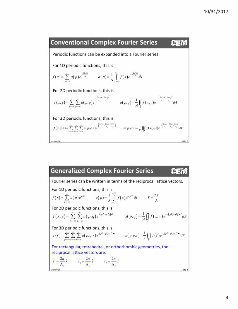
Conventional Complex Fourier Series

Periodic functions can be expanded into a Fourier series.

For 1D periodic functions, this is

22 2

2

1

px pxj j

p

f x a p e a p f x e dx


2 2 2 2

1, , , ,x y x y

px qy px qyj j

p q A

f x y a p q e a p q f x y e dAA


2 2 2 2 2 2

1, , , , , , , ,x y z x y z

px qy rz px qy rzj j

p q r V

f x y z a p q r e a p q r f x y z e dVV

Lecture 18 Slide 8

Generalized Complex Fourier Series

Fourier series can be written in terms of the reciprocal lattice vectors.


2

2

1 2 jpTx jpTx

p

f x a p e a p f x e dx T


1 2 1 21, , , ,

j pT qT r j pT qT r

p q A

f x y a p q e a p q f x y e dAA


1 2 3 1 2 31, , , ,

j pT qT rT r j pT qT rT r

p q r V

f r a p q r e a p q r f r e dVV

For rectangular, tetrahedral, or orthorhombic geometries, the reciprocal lattice vectors are:

1 2 3

2 2 2ˆ ˆ ˆ

x y z

T x T y T z

10/31/2017

5

Lecture 18 Slide 9

Visualizing Expansions with Different ’s

0

0

Lecture 18 Slide 10

Visualizing Expansions with Different Symmetries

Simple‐Cubic Face‐Centered‐Cubic Hexagonal

TriangularSquare

10/31/2017

6

Lecture 18 Slide 11

Starting Point

0

0

0

yzr x

x zr y

y xr z

HHk E

y z

H Hk E

z x

H Hk E

x y

0

0

0

yzr x

x zr y

y xr z

EEk H

y z

E Ek H

z xE E

k Hx y

We start with Maxwell’s equations in the following form…

Recall that we normalized the magnetic field according to

0

0

H j H

Lecture 18 Slide 12

Fourier Expansion of the Materials

1 2 3

1 2 3

, ,

1, ,

j pT qT rT r

rp q r

j pT qT rT r

r

V

r a p q r e

a p q r r e dVV

Assuming the device is infinitely periodic in all directions, the permittivity and permeability functions can be expanded into Fourier Series.

1 2 3

1 2 3

, ,

1, ,

j pT qT rT r

rp q r

j pT qT rT r

r

V

r b p q r e

b p q r r e dVV

10/31/2017

7

Lecture 18 Slide 13

Fourier Expansion of the Fields (1 of 2)

1 2 3, ,j pT qT rT rj r

p q r

E r e S p q r e

The field expansions are slightly different because a wave could be travelling in any direction . The expansions must satisfy the Floquetboundary conditions.

incThink of as k

1 2 3, ,j pT qT rT r

p q r

S p q r e

j re

was brought inside summation and combined with second exponential.Let this be , ,k p q r

1, 2, 3,

1, 2, 3,

1, 2, 3,

, ,

, ,

, ,

x x x x x

y y y y y

z z z z z

k p q r pT qT rT

k p q r pT qT rT

k p q r pT qT rT

, , , , , ,, , x y zj k p q r x k p q r y k p q r z

p q r

S p q r e

1 2 3, ,k p q r pT qT rT

, ,, , jk p q r r

p q r

S p q r e

This is clearly a set of

plane waves with amplitudes . , ,k p q r

Lecture 18 Slide 14

Fourier Expansion of the Fields (2 of 2)

For cubic, tetragonal, and orthorhombic symmetry, the expansions reduce to

, ,

, ,

, ,

x y z

x y z

x y z

j k p x k q y k r z

x xp q r

j k p x k q y k r z

y yp q r

j k p x k q y k r z

z zp q r

E r S p q r e

E r S p q r e

E r S p q r e

2, , , , 2, 1,0,1,2, ,

2, , , , 2, 1,0,1,2, ,

2, , , , 2, 1,0,1, 2, ,

x x xx

y y yy

z z zz

pk p q r k p p

qk p q r k q q

rk p q r k r r

, ,

, ,

, ,

x y z

x y z

x y z

j k p x k q y k r z

x xp q r

j k p x k q y k r z

y yp q r

j k p x k q y k r z

z zp q r

H r U p q r e

H r U p q r e

H r U p q r e

The wave vectors kx, ky, and kz

are still distributed over all possible values of p, q, and r. However, their values only change in one direction, which is conveyed by the argument in parentheses.

Think this way for size of arrays.

Think this way for dependence.

10/31/2017

8

Lecture 18 Slide 15

Substitute Expansions into Maxwell’s Equations

0yz

r x

HHk E

y z

, , x y zj k p x k q y k r z

z zp q r

H r U p q r e


y yp q r

H r U p q r e

2 2 2

, , x y z

p q rj x y z

rp q r

r a p q r e


x xp q r

E r S p q r e

2 2 2

0

, , , ,

, ,

x y z x y z

x y z

j k p x k q y k r z j k p x k q y k r z

z yp q r p q r

p q rj x y z

p q r

U p q r e U p q r ey z

k a p q r e


xp q r

S p q r e

Lecture 18 Slide 16

Algebra for the Left Side Terms

,

, , , ,

, ,

, ,

x y z x y z

x y z

x y z


z zp q r p q r

j k p x k q y k r z

z y pqrp q r

j k p x k q y k r z

y zr

U p q r e U p q r ey y

U p q r jk e

jk q U p q r e

p q

First ugly term…

,

, , , ,

, ,

, ,

x y z x y z

x y z

x y z


y yp q r p q r

j k p x k q y k r z

y z pqrp q r

j k p x k q y k r z

z yr

U p q r e U p q r ez z

U p q r jk e

jk r U p q r e

p q

Second ugly term…

10/31/2017

9

Lecture 18 Slide 17

Algebra for the Right Side Term

2 2 2

, , , ,x y z x y z

p q rj x y z

j k p x k q y k r z

xp q r p q r

a p q r e S p q r e

Here we have the product of two triple summations.

Applying this rule to the triple summations, we get

, , , ,x y zj k p x k q y k r z

xp q r p q r

e a p p q q r r S p q r

Third ugly term…

0 0 0 0

n

n n n n m n mn n n m

a b c c a b

This is called a Cauchy product and is handled as follows.

Lecture 18 Slide 18

Combine the Terms Inside Summation

2 2 2

0

, , , ,

, ,

x y z x y z

x y z


z yp q r p q r

p q rj x y z

p q r

U p q r e U p q r ey z

k a p q r e


xp q r

S p q r e

0

, , , ,

, , , ,

x y z x y z

x y z


y z z yp q r p q r

j k p x k q y k r z

xp q r

jk q U p q r e jk r U p q r e

k e a p p q q r r S p q r

p q r

Our equation can now be brought inside a single triple summation.

0

, , , ,

, , , ,

x y z x y z

x y z


y z z y

j k p x k q y k r zp q r x

p q r



10/31/2017

10

Lecture 18 Slide 19

Final Equation for (p,q,r)th Harmonic

Finally, we divide both sides by the common exponential term and move the j to the right‐hand side.

0

, , , ,

, , , ,

x y z x y z

x y z


y z z y

j k p x k q y k r zp q r x

p q r



0, , , , , , , ,y z z y xp q r

k q U p q r k r U p q r jk a p p q q r r S p q r

0

, , , ,

, , , ,

x y z x y z

x y z


z y y z

j k p x k q y k r z

xp q r

jU p q r k q e jU p q r k r e


The equation inside the braces much be satisfied for each combination of (p,q,r).

Lecture 18 Slide 20

Alternate Derivation

We start with

0yz

r x

HHk E

y z

Point‐by‐point multiplication in real‐space…

We now realized that the strange triple summation remaining in our equation is actually 3D convolution in Fourier space!

, , , ,x xp q r

a S a p p q q r r S p q r

0, , , ,y z z y xk q U p q r k r U p q r jk a S

We Fourier‐transform this equation in x, y, and z resulting in

Our point‐by‐point multiplication becomes a convolution.

FT

FT

r

x x

a

S E

10/31/2017

11

Lecture 18 Slide 21

Maxwell’s Equations in Fourier Space

Real‐Space

0

0

0

, , , , , , , ,

, , , , , , , ,

, , , , , , , ,

y z z y x

z x x z y

x y y x z

k q U p q r k r U p q r jk a p q r S p q r

k r U p q r k p U p q r jk a p q r S p q r

k p U p q r k q U p q r jk a p q r S p q r

Fourier‐Space

0

0

0

yzr x

x zr y

y xr z

HHk E

y z

H Hk E

z x

H Hk E

x y

0

0

0

yzr x

x zr y

y xr z

EEk H

y z

E Ek H

z xE E

k Hx y

0

0

0

, , , , , , , ,

, , , , , , , ,

, , , , , , , ,

y z z y x

z x x z y

x y y x z

k q S p q r k r S p q r jk b p q r U p q r

k r S p q r k p S p q r jk b p q r U p q r

k p S p q r k q S p q r jk b p q r U p q r

2 , , 2, 1,0,1, 2, ,

2 , , 2, 1,0,1, 2, ,

2 , , 2, 1,0,1, 2, ,

x xx

y yy

z zz

pk p p

qk q q

rk r r

Lecture 18 Slide 22

Visualizing Maxwell’s Equations in Fourier Space

In real‐space, we know the field values at discrete points.In Fourier‐space, we know the amplitudes of discrete plane waves.

pq

r

A less clear, but more accurate picture is when all of the plane waves overlap.

10/31/2017

12

Lecture 18 Slide 23

Matrix Form of Maxwell’s Equations in Fourier Space

Lecture 18 Slide 24

Conversion to Matrix Form

The following equation is written once for each spatial harmonic.

This large set of equations can be written in matrix form as

2 2 2

02 2 2

, , , , , , , ,P Q R

y z z y xp P q Q r R

k q U p q r k r U p q r jk a p p q q r r S p q r

0y z z y r xjk K u K u s

1,1,1

1,1,2

, ,

i

ii

i

k

k

k P Q R

K

1,1,1 1,1,1

1,1, 2 1,1, 2

, , , ,

i i

i ii i

i i

U S

U S

U P Q R S P Q R

u s

Toeplitzr

The K terms are diagonal matrices containing all the wave vector components along the center diagonal.

ui and si are column vectors containing the amplitudes of each spatial harmonic in the expansion.

Convolution matrix

Only Toeplitzfor 1D0

0

total # spatial harmonics P Q R

10/31/2017

13

Lecture 18 Slide 25

Matrix Form of Maxwell’s Equations in Fourier Space

Analytical Equations

0

0

0

y z z y r x

z x x z r y

x y y x r z

jk

jk

jk

K u K u s

K u K u s

K u K u s

0

0

0

y z z y r x

z x x z r y

x y y x r z

jk

jk

jk

K s K s u

K s K s u

K s K s u

Numerical Equations

0

0

0

, , , , , , , ,

, , , , , , , ,

, , , , , , , ,

y z z y x

z x x z y

x y y x z

k q U p q r k r U p q r jk a p q r S p q r

k r U p q r k p U p q r jk a p q r S p q r

k p U p q r k q U p q r jk a p q r S p q r

0

0

0

, , , , , , , ,

, , , , , , , ,

, , , , , , , ,

y z z y x

z x x z y

x y y x z

k q S p q r k r S p q r jk b p q r U p q r

k r S p q r k p S p q r jk b p q r U p q r

k p S p q r k q S p q r jk b p q r U p q r

Lecture 18 Slide 26

Interpreting the Column Vectors

Each element of the column vector ui is the complex amplitude of a spatial harmonic.

2

1

0

1

2

i

S

S

S

S

S

s

Column vector

0S

1S

2S

1S

2S

Spatial harmonics

Electric field

10/31/2017

14

Lecture 18 Slide 27

Constructing the Convolution Matrices for Orthorhombic Geometries

Lecture 18 Slide 28

Calculating the Fourier Coefficients

The Fourier coefficients are calculated by solving the following equation for every combination of values of p, q, and r.

2 2 2

1, , x y z

p q rj x y z

r

V

a p q r r e dVV

For cubic, tetragonal, and orthorhombic symmetries, these are easily calculated using a multi‐dimensional Fast Fourier Transform (FFT).

p

q

2D‐FFT ,a p qReal‐Space Fourier‐Space

2a

2a

0

2

a

2

a 0

x

y

p

q

10/31/2017

15

Lecture 18 Slide 29

How Many Points Are Needed on the Real‐Space Grid?

0m

1m

2m

3m

4m

5m

6m

0m

1m

2m

3m

4m

5m

6m

Several hundred in order to accurately calculate the coefficients of the Fourier series.

real

imag

Lecture 18 Slide 30

Convergence of Fourier Coefficients for 2D Functions

Conclusion: when using more spatial harmonics, even more points are needed on the high resolution grid to calculate accurate Fourier coefficients.

10/31/2017

16

Lecture 18 Slide 31

The Convolution Matrix

and r r

There are two matrices that we must construct that perform a 3D convolution in Fourier space.

We construct these matrices with the following picture in mind.

r

, , , ,xp q r

a p p q q r r S p q r

row p,q,r

Constructing the convolution matrices is as simple as placing the Fourier coefficients in the proper order in each row in the matrix.

row 1 1m r PQ q P p

Don’t confuse these for r and r used in FDFD that were diagonal matrices.These will be full convolution matrices.

Lecture 18 Slide 32

Header for MATLAB Code to Construct Convolution Matrices

The following slides will step you through the procedure to write a MATLAB code that calculates convolution matrices for 1D, 2D, or 3D problems. To handle an arbitrary number of dimensions, the header should look like…

function C = convmat(A,P,Q,R)% CONVMAT Rectangular Convolution Matrix%% C = convmat(A,P); for 1D problems% C = convmat(A,P,Q); for 2D problems% C = convmat(A,P,Q,R); for 3D problems%% This MATLAB function constructs convolution matrices% from a real-space grid.

%% HANDLE INPUT AND OUTPUT ARGUMENTS

% DETERMINE SIZE OF A[Nx,Ny,Nz] = size(A);

% HANDLE NUMBER OF HARMONICS FOR ALL DIMENSIONSif nargin==2

Q = 1;R = 1;

elseif nargin==3R = 1;

end

This lets us treat all cases as if they were 3D.

10/31/2017

17

Lecture 18 Slide 33

Step 1: Calculate the Fourier Coefficients

We begin by calculating the indices of the spatial harmonics, centered at 0.% COMPUTE INDICES OF SPATIAL HARMONICSNH = P*Q*R; %total numberp = [-floor(P/2):+floor(P/2)]; %indices along xq = [-floor(Q/2):+floor(Q/2)]; %indices along yr = [-floor(R/2):+floor(R/2)]; %indices along z

number of spatial harmonics along



P x

Q y

R z

Then the Fourier coefficients are calculated using an n‐dimensional FFT.% COMPUTE FOURIER COEFFICIENTS OF AA = fftshift(fftn(A)) / (Nx*Ny*Nz);

We need to calculate the position of the zero‐order harmonic in the array A. Knowing this, all others can be found because they are centered around the zero‐order harmonic.% COMPUTE ARRAY INDICES OF CENTER HARMONICp0 = 1 + floor(Nx/2);q0 = 1 + floor(Ny/2);r0 = 1 + floor(Nz/2);

These equations are valid for both odd and even values of Nx, Ny, and Nz.

P

Q

Lecture 18 Slide 34

Step 2: Initialize Convolution Matrix

The convmat() function will run very slow if the convolution matrix is not first initialized.

% INITIALIZE CONVOLUTION MATRIXC = zeros(NH,NH);

0 0 0

0 0 0

0 0 0

r

10/31/2017

18

r

row p,q,r

Lecture 18 Slide 35

Step 3: Loop Through the Rows

With the picture in mind of filling in rows, it makes sense to start by creating a loop that steps through each row of the convolution matrix.

for rrow = 1 : Rfor qrow = 1 : Qfor prow = 1 : P

row = (rrow-1)*Q*P + (qrow-1)*P + prow;

endendend




P x

Q y

R z

row = 1,2,3,…

r

Lecture 18 Slide 36

Step 4: Loop Through the Columns

Now we step from left to right within the row by looping through the columns.


row = (rrow-1)*Q*P + (qrow-1)*P + prow;for rcol = 1 : Rfor qcol = 1 : Qfor pcol = 1 : P

col = (rcol-1)*Q*P + (qcol-1)*P + pcol;

endendend

endendend




P x

Q y

R z

col = 1,2,3,…

10/31/2017

19

P

Q

Lecture 18 Slide 37

Step 5: Calculate Where to Get Value from FFT

We need to know which Fourier coefficient to place into C(row,col). To determine this, we refer to the original summation that defined the convolution.



col = (rcol-1)*Q*P + (qcol-1)*P + pcol;pfft = p(prow) - p(pcol);qfft = q(qrow) - q(qcol);rfft = r(rrow) - r(rcol);

endendend

endendend




P x

Q y

R z

2 2 2

2 2 2

, , , ,P Q R

xp P q Q r R

a p p q q r r S p q r

fft , fft , fft ,p q ra

r

row p,q,r

Lecture 18 Slide 38

Step 6: Fill in Element of Convolution Matrix

Last, we copy the Fourier coefficient from the n‐FFT into the convolution matrix at element (row,col).



col = (rcol-1)*Q*P + (qcol-1)*P + pcol;pfft = p(prow) - p(pcol);qfft = q(qrow) - q(qcol);rfft = r(rrow) - r(rcol);C(row,col) = A(p0+pfft,q0+qfft,r0+rfft);

endendend

endendend




P x

Q y

R z

We have included the offsets to the zero‐order harmonic.

r

row p,q,r

pfft = qfft = rfft = 0 needs to access the zero‐order harmonic located at p0, q0, r0.

10/31/2017

20

Lecture 18 Slide 39

What Does a Convolution Matrix Look Like?

Device ,r x y

Convolution Matrix• Full matrix• Numbers tend smaller with distance from the center diagonal.

High Resolution Grid• Must be on a very high resolution grid to calculate accurate Fourier coefficients.

Convolution Matrix r

Lecture 18 Slide 40

Convolution Matrices for Homogeneous Media

Device ,r x y Convolution Matrix r

The convolution matrix for a homogeneous material is simply a diagonal matrix with the diagonals all set to r.

r r I

10/31/2017

21

Notes

• You now have a very powerful code!• Most of the tediousness of Fourier space methods are

absorbed into the convolution matrices.• It is able to construct 1D, 2D, and 3D convolution matrices

without changing anything.– For 1D devices: P1, Q=1, R=1– For 2D devices: P1, Q1, R=1– For 3D devices: P1, Q1, R1

• This code can only be used for devices with cubic, tetragonal, and orthorhombic symmetries due to the form of the expansion used.

• Convolution matrices for homogeneous materials are diagonal with the form .

• Uniform directions require only one harmonic.

Lecture 18 Slide 41

r r I

Lecture 18 Slide 42

Fast Fourier Factorization (FFF)

10/31/2017

22

Lecture 18 Slide 43

Product of Two Functions

Suppose we have the product of two periodic functions that have the same period:

f x g x h x

Then we expand each function into its own Fourier series.

2 2 2mx mx mxj j j

m m mm m m

a e b e c e

This is exact as long as an infinite number of terms is used.

Obviously, only a finite number of terms can be retained in the expansion if it is to be solved on a computer.

Lecture 18 Slide 44

Finite Number of Terms

To describe devices on a computer, we can retain only a finite number of terms

2 2 2mx mx mxM M Mj j j

m m mm M m M m M

a e b e c e

We have four special cases for :

1. f(x) and g(x) are continuous everywhere.2. Either f(x) or g(x) has a step discontinuity, but not

both at the same point.3. Both f(x) and g(x) have a step discontinuity at the

same point, but their product is continuous.4. Both f(x) and g(x) have a step discontinuity at the

same point and their product is also discontinuous.

When we retain only a finite‐number of terms, cases 3 and 4 exhibit slow convergence. Only case 3 is fixable.

Problem: the left side of the equation converges slower than the right. That is, more terms are needed for a given level of “accuracy.”

f x g x h x

No problem

Problem is fixable

Problem is NOT fixable

10/31/2017

23

Lecture 18 Slide 45

The Fix for Case 3

We can write our product of two functions in Fourier space.

f g h F G H

For Case 3, both f(x) and g(x) are have a step discontinuity at the same point, but their product f(x)g(x)=h(x) is continuous. To handle this case, we bring f(x) to the right‐hand side of the equation.

1 1 g h G H

f F

Now, there are no problems with this new equation because both sides of the equation are Case 2. We bring the convolution matrix back to left side of the equation.

1 1

1 1 g h G H

f F

Lecture 18 Slide 46

Convergence Problem with Finite Terms

f x

g x

idealh x

No FFFh x

FFFh x

Fast convergence Slow convergence Fast convergence again!

10/31/2017

24

Lecture 18 Slide 47

FFF and Maxwell’s Equations

In Maxwell’s equations, we have the product of two functions…

r r E r

The dielectric function is discontinuous at the interface between two materials. Boundary conditions require that

1,|| 2,||E E

1 1, 2 2,E E

Tangential component is continuous across the interface

Normal component is discontinuous across the interface, but the product of is continuous.

We conclude that we must handle the convolution matrix differently for the tangential and normal components. This implies that the final convolution matrix will be a tensor.

E

Lecture 18 Slide 48

FFF for Maxwell’s Equations

First, we decompose the electric field into tangential and normal components at all interfaces.

|| ||r r r r s s s s s

,|

1

,F | |FF | 1r rr

s ss

We now have the opportunity to associate different convolution matrices with the different field components.

,|| | ,|r rr sss Case 2.No problems.

Case 3.Fixable with FFF.

10/31/2017

25

Lecture 18 Slide 49

Normal Vector Field

To implement FFF, we must determine what directions are parallel and perpendicular at each point in space.

For arbitrarily shaped devices, this comes from knowledge of the materials within the layer.

We must construct a vector function throughout the grid that is normal to all the interfaces. This called the “normal vector” field.

ˆ , ,n x y z

P. Gotz, T. Schuster, K. Frenner, S. Rafler, W. Osten, “Normal vector method for the RCWA with automated vector field generation,” Opt. Express 16(22), 17295‐17301 (2008).

This can be very difficult to calculate!!

Lecture 18 Slide 50

Incorporating Normal Vector Function

Recall the FFF fix

1

||FFF1r r r

s s s

||

s Ns

s s Ns I N s

The parallel and perpendicular components of s can be calculated using the normal vector matrix N.

Substituting these into the FFF equation yields

1

FFF

1

1

1

1

1

r r r

r r r

r r r

s I N s Ns

s Ns Ns

N N s

This defines a new convolution matrix that incorporates FFF.

10/31/2017

26

Lecture 18 Slide 51

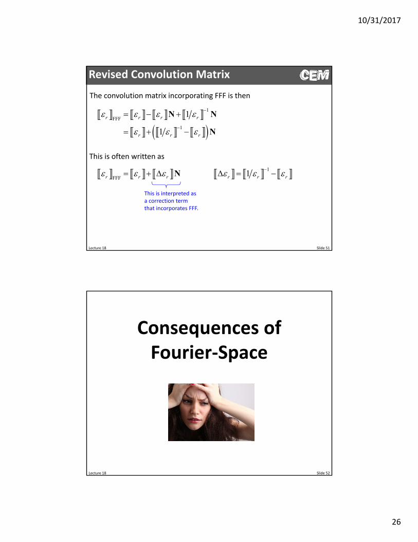
Revised Convolution Matrix

The convolution matrix incorporating FFF is then

1

FFF

1

1

1

r r r r

r r r

N N

N

This is often written as

FFFr r r N 11r r r

This is interpreted as a correction term that incorporates FFF.

Lecture 18 Slide 52

Consequences of Fourier‐Space

10/31/2017

27

Lecture 18 Slide 53

Efficient Representation of Devices

3×3 7×7 11×11 15×15 19×19 23×23 27×27 31×31 35×35 39×39

Along a given direction, approximately half the number of the terms are needed in Fourier space than would be needed in real space.

For 2D problems in real space, 4× more terms are needed making the matrices 16× larger.

For 3D problems in real space, 8× more terms are needed making the matrices 64× larger.

Lecture 18 Slide 54

Blurring from Too Few Harmonics

If too few harmonics are used, the geometry of the device is blurred.

• Boundaries are artificially blurred.• Reflections at boundaries are artificially reduced.• It is difficult or impossible to resolve fine features or rapidly varying fields.

1×1 3×3 5×5 7×7

11×11 21×21 41×41 81×81

Rule of Thumb: # harmonics = 10 per

10/31/2017

28

Lecture 18 Slide 55

Gibb’s Phenomena

A problem occurs when a discontinuous function (material interface) is represented by continuous basis functions (sin’s and cos’s). When the Fourier transform is used, “spikes” appear around each discontinuity. Fourier space methods act is if those spikes are actually present.

0

2 sin1.1789797445

xdx

x

http://mathworld.wolfram.com/GibbsPhenomenon.html

Lecture 18 Slide 56

Gibb’s Phenomena in Maxwell’s Equations

A Fourier‐space numerical method treats the spikes as if they are real.

• The magnitude of the spikes remains constant no matter how many harmonics are used.• The magnitude of the spikes is proportional to the severity of the discontinuity.• The width of the spikes becomes more narrow with increasing number of harmonics.• In Fourier‐space, Maxwell’s equations really think the spikes are there.

11×11 21×21 41×41 81×81

1×1 3×3 5×5 7×7

Due to Gibb’s phenomenon, Fourier‐space analysis is most efficient for structures with low to moderate index contrast, but many people have modeled metals effectively.

lecture 18 -- maxwell's equations in fourier spaceemlab.utep.edu/ee5390cem/lecture 18 --...

Documents