maxwell's equations - ecuaciones de maxwell libro

http://www.cambridge.org/9780521877619

This page intentionally left blank

A Student’s Guide to Maxwell’s Equations

Maxwell’s Equations are four of the most influential equations in science: Gauss’s

law for electric fields, Gauss’s law for magnetic fields, Faraday’s law, and the

Ampere–Maxwell law. In this guide for students, each equation is the subject of

an entire chapter, with detailed, plain-language explanations of the physical

meaning of each symbol in the equation, for both the integral and differential

forms. The final chapter shows how Maxwell’s Equations may be combined to

produce the wave equation, the basis for the electromagnetic theory of light.

This book is a wonderful resource for undergraduate and graduate courses in

electromagnetism and electromagnetics. A website hosted by the author, and

available through www.cambridge.org/9780521877619, contains interactive

solutions to every problem in the text. Entire solutions can be viewed

immediately, or a series of hints can be given to guide the student to the final

answer. The website also contains audio podcasts which walk students through

each chapter, pointing out important details and explaining key concepts.

daniel fleisch is Associate Professor in the Department of Physics at

Wittenberg University, Ohio. His research interests include radar cross-section

measurement, radar system analysis, and ground-penetrating radar. He is a

member of the American Physical Society (APS), the American Association of

Physics Teachers (AAPT), and the Institute of Electrical and Electronics

Engineers (IEEE).

www.cambridge.org/9780521877619

A Student’s Guide to

Maxwell’s Equations

DANIEL FLEISCH

Wittenberg University

CAMBRIDGE UNIVERSITY PRESS

Cambridge, New York, Melbourne, Madrid, Cape Town, Singapore, São Paulo

Cambridge University PressThe Edinburgh Building, Cambridge CB2 8RU, UK

First published in print format

ISBN-13 978-0-521-87761-9

ISBN-13 978-0-511-39308-2

© D. Fleisch 2008

2008

Information on this title: www.cambridge.org/9780521877619

This publication is in copyright. Subject to statutory exception and to the provision of relevant collective licensing agreements, no reproduction of any part may take place without the written permission of Cambridge University Press.

Cambridge University Press has no responsibility for the persistence or accuracy of urls for external or third-party internet websites referred to in this publication, and does not guarantee that any content on such websites is, or will remain, accurate or appropriate.

Published in the United States of America by Cambridge University Press, New York

www.cambridge.org

eBook (EBL)

hardback

http://www.cambridge.org/9780521877619

http://www.cambridge.org

Contents

Preface page vii

Acknowledgments ix

1 Gauss’s law for electric fields 1

1.1 The integral form of Gauss’s law 1

The electric field 3

The dot product 6

The unit normal vector 7

The component of ~E normal to a surface 8

The surface integral 9

The flux of a vector field 10

The electric flux through a closed surface 13

The enclosed charge 16

The permittivity of free space 18

Applying Gauss’s law (integral form) 20

1.2 The differential form of Gauss’s law 29

Nabla – the del operator 31

Del dot – the divergence 32

The divergence of the electric field 36

Applying Gauss’s law (differential form) 38

2 Gauss’s law for magnetic fields 43

2.1 The integral form of Gauss’s law 43

The magnetic field 45

The magnetic flux through a closed surface 48

Applying Gauss’s law (integral form) 50

2.2 The differential form of Gauss’s law 53

The divergence of the magnetic field 54

Applying Gauss’s law (differential form) 55

v

3 Faraday’s law 58

3.1 The integral form of Faraday’s law 58

The induced electric field 62

The line integral 64

The path integral of a vector field 65

The electric field circulation 68

The rate of change of flux 69

Lenz’s law 71

Applying Faraday’s law (integral form) 72

3.2 The differential form of Faraday’s law 75

Del cross – the curl 76

The curl of the electric field 79

Applying Faraday’s law (differential form) 80

4 The Ampere–Maxwell law 83

4.1 The integral form of the Ampere–Maxwell law 83

The magnetic field circulation 85

The permeability of free space 87

The enclosed electric current 89

The rate of change of flux 91

Applying the Ampere–Maxwell law (integral form) 95

4.2 The differential form of the Ampere–Maxwell law 101

The curl of the magnetic field 102

The electric current density 105

The displacement current density 107

Applying the Ampere–Maxwell law (differential form) 108

5 From Maxwell’s Equations to the wave equation 112

The divergence theorem 114

Stokes’ theorem 116

The gradient 119

Some useful identities 120

The wave equation 122

Appendix: Maxwell’s Equations in matter 125

Further reading 131

Index 132

Contentsvi

Preface

This book has one purpose: to help you understand four of the mostinfluential equations in all of science. If you need a testament to thepower of Maxwell’s Equations, look around you – radio, television,radar, wireless Internet access, and Bluetooth technology are a fewexamples of contemporary technology rooted in electromagnetic fieldtheory. Little wonder that the readers of Physics World selected Maxwell’sEquations as “the most important equations of all time.”

How is this book different from the dozens of other texts on electricityand magnetism? Most importantly, the focus is exclusively on Maxwell’sEquations, which means you won’t have to wade through hundreds ofpages of related topics to get to the essential concepts. This leaves roomfor in-depth explanations of the most relevant features, such as the dif-ference between charge-based and induced electric fields, the physicalmeaning of divergence and curl, and the usefulness of both the integraland differential forms of each equation.

You’ll also find the presentation to be very different from that of otherbooks. Each chapter begins with an “expanded view” of one of Maxwell’sEquations, in which the meaning of each term is clearly called out. Ifyou’ve already studied Maxwell’s Equations and you’re just looking for aquick review, these expanded views may be all you need. But if you’re abit unclear on any aspect of Maxwell’s Equations, you’ll find a detailedexplanation of every symbol (including the mathematical operators) inthe sections following each expanded view. So if you’re not sure of themeaning of ~E � n in Gauss’s Law or why it is only the enclosed currentsthat contribute to the circulation of the magnetic field, you’ll want to readthose sections.

As a student’s guide, this book comes with two additional resourcesdesigned to help you understand and apply Maxwell’s Equations: aninteractive website and a series of audio podcasts. On the website, you’llfind the complete solution to every problem presented in the text in

vii

interactive format – which means that you’ll be able to view the entiresolution at once, or ask for a series of helpful hints that will guide you tothe final answer. And if you’re the kind of learner who benefits fromhearing spoken words rather than just reading text, the audio podcasts arefor you. These MP3 files walk you through each chapter of the book,pointing out important details and providing further explanations of keyconcepts.

Is this book right for you? It is if you’re a science or engineeringstudent who has encountered Maxwell’s Equations in one of your text-books, but you’re unsure of exactly what they mean or how to use them.In that case, you should read the book, listen to the accompanyingpodcasts, and work through the examples and problems before taking astandardized test such as the Graduate Record Exam. Alternatively, ifyou’re a graduate student reviewing for your comprehensive exams, thisbook and the supplemental materials will help you prepare.

And if you’re neither an undergraduate nor a graduate science student,but a curious young person or a lifelong learner who wants to know moreabout electric and magnetic fields, this book will introduce you to thefour equations that are the basis for much of the technology you useevery day.

The explanations in this book are written in an informal style in whichmathematical rigor is maintained only insofar as it doesn’t get in the wayof understanding the physics behind Maxwell’s Equations. You’ll findplenty of physical analogies – for example, comparison of the flux ofelectric and magnetic fields to the flow of a physical fluid. James ClerkMaxwell was especially keen on this way of thinking, and he was carefulto point out that analogies are useful not because the quantities are alikebut because of the corresponding relationships between quantities. Soalthough nothing is actually flowing in a static electric field, you’re likelyto find the analogy between a faucet (as a source of fluid flow) andpositive electric charge (as the source of electric field lines) very helpful inunderstanding the nature of the electrostatic field.

One final note about the four Maxwell’s Equations presented in thisbook: it may surprise you to learn that whenMaxwell worked out his theoryof electromagnetism, he ended up with not four but twenty equations thatdescribe the behavior of electric andmagnetic fields. It was Oliver Heavisidein Great Britain and Heinrich Hertz in Germany who combined and sim-plified Maxwell’s Equations into four equations in the two decades afterMaxwell’s death. Todaywe call these four equations Gauss’s law for electricfields, Gauss’s law for magnetic fields, Faraday’s law, and the Ampere–Maxwell law. Since these four laws are now widely defined as Maxwell’sEquations, they are the ones you’ll find explained in the book.

Prefaceviii

Acknowledgments

This book is the result of a conversation with the great Ohio State radioastronomer John Kraus, who taught me the value of plain explanations.Professor Bill Dollhopf of Wittenberg University provided helpful sug-gestions on the Ampere–Maxwell law, and postdoc Casey Miller of theUniversity of Texas did the same for Gauss’s law. The entire manuscriptwas reviewed by UC Berkeley graduate student Julia Kregenow andWittenberg undergraduate Carissa Reynolds, both of whom made sig-nificant contributions to the content as well as the style of this work.Daniel Gianola of Johns Hopkins University and Wittenberg graduateMelanie Runkel helped with the artwork. The Maxwell Foundation ofEdinburgh gave me a place to work in the early stages of this project, andCambridge University made available their extensive collection of JamesClerk Maxwell’s papers. Throughout the development process, Dr. JohnFowler of Cambridge University Press has provided deft guidance andpatient support.

ix

1

Gauss’s law for electric fields

In Maxwell’s Equations, you’ll encounter two kinds of electric field: the

electrostatic field produced by electric charge and the induced electric field

produced by a changing magnetic field. Gauss’s law for electric fields

deals with the electrostatic field, and you’ll find this law to be a powerful

tool because it relates the spatial behavior of the electrostatic field to the

charge distribution that produces it.

1.1 The integral form of Gauss’s law

There are many ways to express Gauss’s law, and although notation

differs among textbooks, the integral form is generally written like this:IS

~E � n da ¼ qenc

e0Gauss’s law for electric fields (integral form).

The left side of this equation is no more than a mathematical description

of the electric flux – the number of electric field lines – passing through a

closed surface S, whereas the right side is the total amount of charge

contained within that surface divided by a constant called the permittivity

of free space.

If you’re not sure of the exact meaning of ‘‘field line’’ or ‘‘electric flux,’’

don’t worry – you can read about these concepts in detail later in this

chapter. You’ll also find several examples showing you how to use

Gauss’s law to solve problems involving the electrostatic field. For

starters, make sure you grasp the main idea of Gauss’s law:

Electric charge produces an electric field, and the flux of that field

passing through any closed surface is proportional to the total charge

contained within that surface.

1

In other words, if you have a real or imaginary closed surface of any size

and shape and there is no charge inside the surface, the electric flux

through the surface must be zero. If you were to place some positive

charge anywhere inside the surface, the electric flux through the surface

would be positive. If you then added an equal amount of negative charge

inside the surface (making the total enclosed charge zero), the flux would

again be zero. Remember that it is the net charge enclosed by the surface

that matters in Gauss’s law.

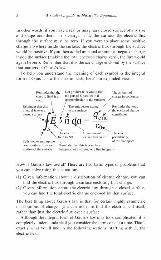
To help you understand the meaning of each symbol in the integral

form of Gauss’s law for electric fields, here’s an expanded view:

How is Gauss’s law useful? There are two basic types of problems that

you can solve using this equation:

(1) Given information about a distribution of electric charge, you can

find the electric flux through a surface enclosing that charge.

(2) Given information about the electric flux through a closed surface,

you can find the total electric charge enclosed by that surface.

The best thing about Gauss’s law is that for certain highly symmetric

distributions of charges, you can use it to find the electric field itself,

rather than just the electric flux over a surface.

Although the integral form of Gauss’s law may look complicated, it is

completely understandable if you consider the terms one at a time. That’s

exactly what you’ll find in the following sections, starting with ~E, the

electric field.

ˆ �0=

S

qencdanE

Reminder that thisintegral is over aclosed surface

The electricfield in N/C

Reminder that this is a surfaceintegral (not a volume or a line integral)

Reminder that theelectric field is avector

The unit vector normalto the surface

The amount of charge in coulombs

Reminder that onlythe enclosed chargecontributes

An increment ofsurface area in m2

Tells you to sum up thecontributions from eachportion of the surface

The electricpermittivityof the free space

Dot product tells you to findthe part of E parallel to n(perpendicular to the surface)

ˆ

∫

A student’s guide to Maxwell’s Equations2

~E The electric field

To understand Gauss’s law, you first have to understand the concept of

the electric field. In some physics and engineering books, no direct def-

inition of the electric field is given; instead you’ll find a statement that an

electric field is ‘‘said to exist’’ in any region in which electrical forces act.

But what exactly is an electric field?

This question has deep philosophical significance, but it is not easy to

answer. It was Michael Faraday who first referred to an electric ‘‘field of

force,’’ and James Clerk Maxwell identified that field as the space around

an electrified object – a space in which electric forces act.

The common thread running through most attempts to define the

electric field is that fields and forces are closely related. So here’s a very

pragmatic definition: an electric field is the electrical force per unit charge

exerted on a charged object. Although philosophers debate the true

meaning of the electric field, you can solve many practical problems by

thinking of the electric field at any location as the number of newtons of

electrical force exerted on each coulomb of charge at that location. Thus,

the electric field may be defined by the relation

~E �~Fe

q0; ð1:1Þ

where ~Fe is the electrical force on a small1 charge q0. This definition

makes clear two important characteristics of the electric field:

(1) ~E is a vector quantity with magnitude directly proportional to force

and with direction given by the direction of the force on a positive

test charge.

(2) ~E has units of newtons per coulomb (N/C), which are the same as

volts per meter (V/m), since volts¼ newtons ·meters/coulombs.

In applying Gauss’s law, it is often helpful to be able to visualize the

electric field in the vicinity of a charged object. The most common

approaches to constructing a visual representation of an electric field are

to use a either arrows or ‘‘field lines’’ that point in the direction of

the field at each point in space. In the arrow approach, the strength of the

field is indicated by the length of the arrow, whereas in the field line

1 Why do physicists and engineers always talk about small test charges? Because the job ofthis charge is to test the electric field at a location, not to add another electric field into themix (although you can’t stop it from doing so). Making the test charge infinitesimallysmall minimizes the effect of the test charge’s own field.

Gauss’s law for electric fields 3

approach, it is the spacing of the lines that tells you the field strength

(with closer lines signifying a stronger field). When you look at a drawing

of electric field lines or arrows, be sure to remember that the field exists

between the lines as well.

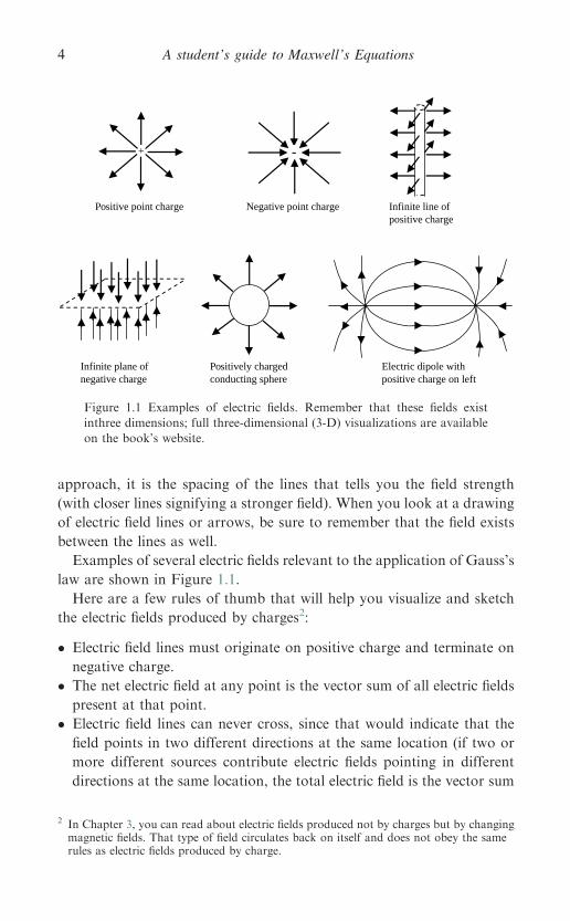
Examples of several electric fields relevant to the application of Gauss’s

law are shown in Figure 1.1.

Here are a few rules of thumb that will help you visualize and sketch

the electric fields produced by charges2:

� Electric field lines must originate on positive charge and terminate on

negative charge.

� The net electric field at any point is the vector sum of all electric fields

present at that point.

� Electric field lines can never cross, since that would indicate that the

field points in two different directions at the same location (if two or

more different sources contribute electric fields pointing in different

directions at the same location, the total electric field is the vector sum

Positive point charge Negative point charge Infinite line ofpositive charge

Infinite plane ofnegative charge

Positively chargedconducting sphere

Electric dipole withpositive charge on left

+ -

Figure 1.1 Examples of electric fields. Remember that these fields exist

inthree dimensions; full three-dimensional (3-D) visualizations are available

on the book’s website.

2 In Chapter 3, you can read about electric fields produced not by charges but by changingmagnetic fields. That type of field circulates back on itself and does not obey the samerules as electric fields produced by charge.


of the individual fields, and the electric field lines always point in the

single direction of the total field).

� Electric field lines are always perpendicular to the surface of a

conductor in equilibrium.

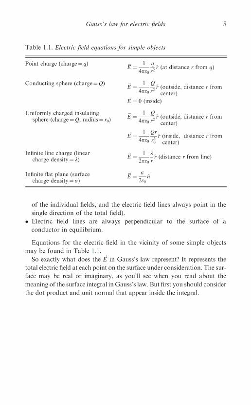
Equations for the electric field in the vicinity of some simple objects

may be found in Table 1.1.

So exactly what does the ~E in Gauss’s law represent? It represents the

total electric field at each point on the surface under consideration. The sur-

face may be real or imaginary, as you’ll see when you read about the

meaning of the surface integral in Gauss’s law. But first you should consider

the dot product and unit normal that appear inside the integral.

Table 1.1. Electric field equations for simple objects

Point charge (charge¼ q) ~E ¼ 1

4pe0

q

r2r (at distance r from q)

Conducting sphere (charge¼Q) ~E ¼ 1

4pe0

Q

r2r (outside, distance r fromcenter)

~E ¼ 0 (inside)

Uniformly charged insulatingsphere (charge¼Q, radius¼ r0)

~E ¼ 1

4pe0

Q

r2r (outside, distance r fromcenter)

~E ¼ 1

4pe0

Qr

r30r (inside, distance r fromcenter)

Infinite line charge (linearcharge density¼ k)

~E ¼ 1

2pe0

krr (distance r from line)

Infinite flat plane (surfacecharge density¼ r)

~E ¼ r2e0

n


� The dot product

When you’re dealing with an equation that contains a multiplication

symbol (a circle or a cross), it is a good idea to examine the terms on

both sides of that symbol. If they’re printed in bold font or are wearing

vector hats (as are ~E and n in Gauss’s law), the equation involves vector

multiplication, and there are several different ways to multiply vectors

(quantities that have both magnitude and direction).

In Gauss’s law, the circle between ~E and n represents the dot product

(or ‘‘scalar product’’) between the electric field vector ~E and the unit

normal vector n (discussed in the next section). If you know the Cartesian

components of each vector, you can compute this as

~A � ~B ¼ AxBx þ AyBy þ AzBz: ð1:2ÞOr, if you know the angle h between the vectors, you can use

~A �~B ¼ j~Ajj~Bj cos h; ð1:3Þ

where j~Aj and j~Bj represent the magnitude (length) of the vectors. Notice

that the dot product between two vectors gives a scalar result.

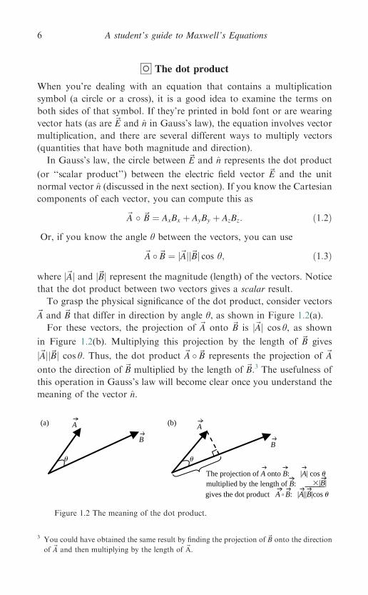
To grasp the physical significance of the dot product, consider vectors

~A and ~B that differ in direction by angle h, as shown in Figure 1.2(a).

For these vectors, the projection of ~A onto ~B is j~Aj cos h, as shown

in Figure 1.2(b). Multiplying this projection by the length of ~B gives

j~Ajj~Bj cos h. Thus, the dot product ~A �~B represents the projection of ~A

onto the direction of ~B multiplied by the length of ~B.3 The usefulness of

this operation in Gauss’s law will become clear once you understand the

meaning of the vector n.

A(a) (b) A

BB

u u

The projection of A onto B: |A| cos umultiplied by the length of B: 3|B|

gives the dot product A B: |A||B|cos u

Figure 1.2 The meaning of the dot product.

3 You could have obtained the same result by finding the projection of ~B onto the direction

of ~A and then multiplying by the length of ~A.


n The unit normal vector

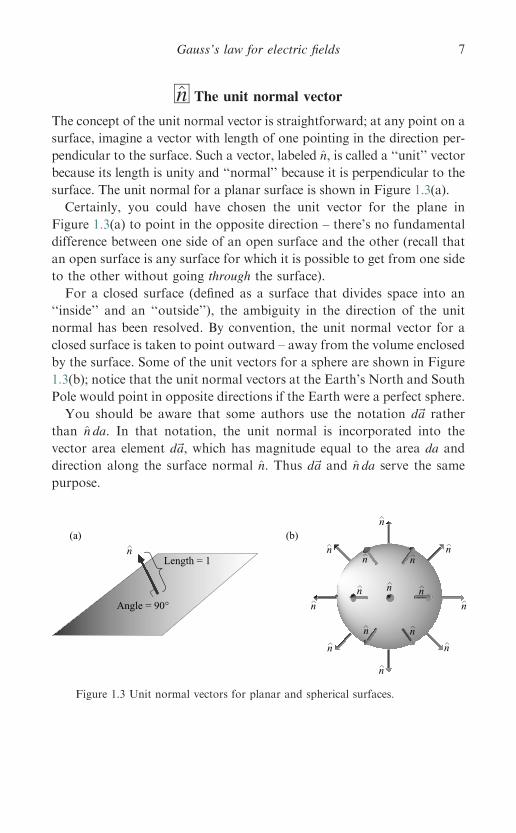
The concept of the unit normal vector is straightforward; at any point on a

surface, imagine a vector with length of one pointing in the direction per-

pendicular to the surface. Such a vector, labeled n, is called a ‘‘unit’’ vector

because its length is unity and ‘‘normal’’ because it is perpendicular to the

surface. The unit normal for a planar surface is shown in Figure 1.3(a).

Certainly, you could have chosen the unit vector for the plane in

Figure 1.3(a) to point in the opposite direction – there’s no fundamental

difference between one side of an open surface and the other (recall that

an open surface is any surface for which it is possible to get from one side

to the other without going through the surface).

For a closed surface (defined as a surface that divides space into an

‘‘inside’’ and an ‘‘outside’’), the ambiguity in the direction of the unit

normal has been resolved. By convention, the unit normal vector for a

closed surface is taken to point outward – away from the volume enclosed

by the surface. Some of the unit vectors for a sphere are shown in Figure

1.3(b); notice that the unit normal vectors at the Earth’s North and South

Pole would point in opposite directions if the Earth were a perfect sphere.

You should be aware that some authors use the notation d~a rather

than n da. In that notation, the unit normal is incorporated into the

vector area element d~a, which has magnitude equal to the area da and

direction along the surface normal n. Thus d~a and n da serve the same

purpose.

Figure 1.3 Unit normal vectors for planar and spherical surfaces.


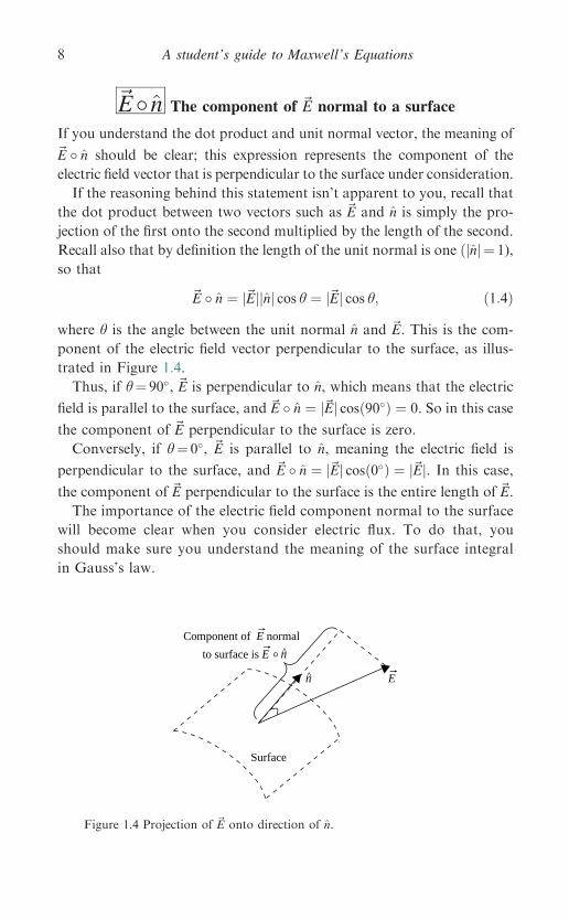
~E� n The component of ~E normal to a surface

If you understand the dot product and unit normal vector, the meaning of

~E � n should be clear; this expression represents the component of the

electric field vector that is perpendicular to the surface under consideration.

If the reasoning behind this statement isn’t apparent to you, recall that

the dot product between two vectors such as ~E and n is simply the pro-

jection of the first onto the second multiplied by the length of the second.

Recall also that by definition the length of the unit normal is one ðjnj ¼ 1),

so that

~E � n ¼ j~Ejjnj cos h ¼ j~Ej cos h; ð1:4Þwhere h is the angle between the unit normal n and ~E. This is the com-

ponent of the electric field vector perpendicular to the surface, as illus-

trated in Figure 1.4.

Thus, if h¼ 90�, ~E is perpendicular to n, which means that the electric

field is parallel to the surface, and ~E � n ¼ j~Ej cosð90�Þ ¼ 0. So in this case

the component of ~E perpendicular to the surface is zero.

Conversely, if h¼ 0�, ~E is parallel to n, meaning the electric field is

perpendicular to the surface, and ~E � n ¼ j~Ej cosð0�Þ ¼ j~Ej. In this case,

the component of ~E perpendicular to the surface is the entire length of ~E.

The importance of the electric field component normal to the surface

will become clear when you consider electric flux. To do that, you

should make sure you understand the meaning of the surface integral

in Gauss’s law.

n E

Component of E normal

to surface is E n

Surface

^

^

Figure 1.4 Projection of ~E onto direction of n.


RSðÞda The surface integral

Many equations in physics and engineering – Gauss’s law among them –

involve the area integral of a scalar function or vector field over a spe-

cified surface (this type of integral is also called the ‘‘surface integral’’).

The time you spend understanding this important mathematical oper-

ation will be repaid many times over when you work problems in

mechanics, fluid dynamics, and electricity and magnetism (E&M).

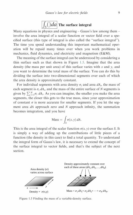
The meaning of the surface integral can be understood by considering a

thin surface such as that shown in Figure 1.5. Imagine that the area

density (the mass per unit area) of this surface varies with x and y, and

you want to determine the total mass of the surface. You can do this by

dividing the surface into two-dimensional segments over each of which

the area density is approximately constant.

For individual segments with area density ri and area dAi, the mass of

each segment is ri dAi, and the mass of the entire surface of N segments is

given byP

Ni¼1ri dAi. As you can imagine, the smaller you make the area

segments, the closer this gets to the true mass, since your approximation

of constant r is more accurate for smaller segments. If you let the seg-

ment area dA approach zero and N approach infinity, the summation

becomes integration, and you have

Mass ¼ZS

rðx; yÞ dA:

This is the area integral of the scalar function r(x, y) over the surface S. Itis simply a way of adding up the contributions of little pieces of a

function (the density in this case) to find a total quantity. To understand

the integral form of Gauss’s law, it is necessary to extend the concept of

the surface integral to vector fields, and that’s the subject of the next

section.

Area density (s)varies across surface

Density approximately constant overeach of these areas (dA1, dA2, . . . , dAN)

s1 s2 s3

sΝ

Density = s(x,y) Mass = s1 dA1+ s2 dA2+ . . . + sN dAN. x

y

Figure 1.5 Finding the mass of a variable-density surface.


Rs~A � n da The flux of a vector field

In Gauss’s law, the surface integral is applied not to a scalar function

(such as the density of a surface) but to a vector field. What’s a vector

field? As the name suggests, a vector field is a distribution of quantities in

space – a field – and these quantities have both magnitude and direction,

meaning that they are vectors. So whereas the distribution of temperature

in a room is an example of a scalar field, the speed and direction of the

flow of a fluid at each point in a stream is an example of a vector field.

The analogy of fluid flow is very helpful in understanding the meaning

of the ‘‘flux’’ of a vector field, even when the vector field is static and

nothing is actually flowing. You can think of the flux of a vector field

over a surface as the ‘‘amount’’ of that field that ‘‘flows’’ through that

surface, as illustrated in Figure 1.6.

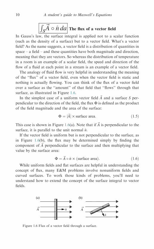
In the simplest case of a uniform vector field ~A and a surface S per-

pendicular to the direction of the field, the flux U is defined as the product

of the field magnitude and the area of the surface:

U ¼ j~Aj · surface area: ð1:5Þ

This case is shown in Figure 1.6(a). Note that if ~A is perpendicular to the

surface, it is parallel to the unit normal n:

If the vector field is uniform but is not perpendicular to the surface, as

in Figure 1.6(b), the flux may be determined simply by finding the

component of ~A perpendicular to the surface and then multiplying that

value by the surface area:

U ¼ ~A � n · ðsurface areaÞ: ð1:6ÞWhile uniform fields and flat surfaces are helpful in understanding the

concept of flux, many E&M problems involve nonuniform fields and

curved surfaces. To work those kinds of problems, you’ll need to

understand how to extend the concept of the surface integral to vector

fields.

n

n

A

(a) (b)

A

Figure 1.6 Flux of a vector field through a surface.


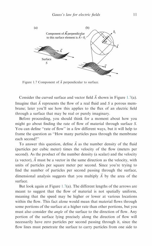
Consider the curved surface and vector field ~A shown in Figure 1.7(a).

Imagine that ~A represents the flow of a real fluid and S a porous mem-

brane; later you’ll see how this applies to the flux of an electric field

through a surface that may be real or purely imaginary.

Before proceeding, you should think for a moment about how you

might go about finding the rate of flow of material through surface S.

You can define ‘‘rate of flow’’ in a few different ways, but it will help to

frame the question as ‘‘How many particles pass through the membrane

each second?’’

To answer this question, define ~A as the number density of the fluid

(particles per cubic meter) times the velocity of the flow (meters per

second). As the product of the number density (a scalar) and the velocity

(a vector), ~A must be a vector in the same direction as the velocity, with

units of particles per square meter per second. Since you’re trying to

find the number of particles per second passing through the surface,

dimensional analysis suggests that you multiply ~A by the area of the

surface.

But look again at Figure 1.7(a). The different lengths of the arrows are

meant to suggest that the flow of material is not spatially uniform,

meaning that the speed may be higher or lower at various locations

within the flow. This fact alone would mean that material flows through

some portions of the surface at a higher rate than other portions, but you

must also consider the angle of the surface to the direction of flow. Any

portion of the surface lying precisely along the direction of flow will

necessarily have zero particles per second passing through it, since the

flow lines must penetrate the surface to carry particles from one side to

u

ni

A

AA

A

SurfaceS

(a) (b)

Component of A perpendicularto this surface element is A ° ni

Figure 1.7 Component of ~A perpendicular to surface.


the other. Thus, you must be concerned not only with the speed of flow

and the area of each portion of the membrane, but also with the com-

ponent of the flow perpendicular to the surface.

Of course, you know how to find the component of ~A perpendicular

to the surface; simply form the dot product of~A and n, the unit normal to

the surface. But since the surface is curved, the direction of n depends on

which part of the surface you’re considering. To deal with the different n

(and ~A) at each location, divide the surface into small segments, as shown

in Figure 1.7(b). If you make these segments sufficiently small, you can

assume that both n and ~A are constant over each segment.

Let ni represent the unit normal for the ith segment (of area dai); the

flow through segment i is (~Ai � ni) dai, and the total is

flow through entire surface¼Pi

~Ai � ni dai:

It should come as no surprise that if you now let the size of each

segment shrink to zero, the summation becomes integration.

Flow through entire surface ¼ZS

~A � n da: ð1:7Þ

For a closed surface, the integral sign includes a circle:IS

~A � n da: ð1:8Þ

This flow is the particle flux through a closed surface S, and the similarity

to the left side of Gauss’s law is striking. You have only to replace the

vector field ~A with the electric field ~E to make the expressions identical.


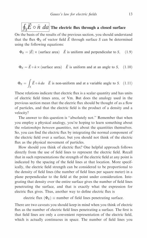
HS~E � n da The electric flux through a closed surface

On the basis of the results of the previous section, you should understand

that the flux UE of vector field ~E through surface S can be determined

using the following equations:

UE ¼ j~Ej · ðsurface areaÞ ~E is uniform and perpendicular to S; ð1:9Þ

UE ¼ ~E � n · ðsurface areaÞ ~E is uniform and at an angle to S; ð1:10Þ

UE ¼ZS

~E � n da ~E is non-uniform and at a variable angle to S: ð1:11Þ

These relations indicate that electric flux is a scalar quantity and has units

of electric field times area, or Vm. But does the analogy used in the

previous section mean that the electric flux should be thought of as a flow

of particles, and that the electric field is the product of a density and a

velocity?

The answer to this question is ‘‘absolutely not.’’ Remember that when

you employ a physical analogy, you’re hoping to learn something about

the relationships between quantities, not about the quantities themselves.

So, you can find the electric flux by integrating the normal component of

the electric field over a surface, but you should not think of the electric

flux as the physical movement of particles.

How should you think of electric flux? One helpful approach follows

directly from the use of field lines to represent the electric field. Recall

that in such representations the strength of the electric field at any point is

indicated by the spacing of the field lines at that location. More specif-

ically, the electric field strength can be considered to be proportional to

the density of field lines (the number of field lines per square meter) in a

plane perpendicular to the field at the point under consideration. Inte-

grating that density over the entire surface gives the number of field lines

penetrating the surface, and that is exactly what the expression for

electric flux gives. Thus, another way to define electric flux is

electric flux ðUEÞ � number of field lines penetrating surface.

There are two caveats you should keep in mind when you think of electric

flux as the number of electric field lines penetrating a surface. The first is

that field lines are only a convenient representation of the electric field,

which is actually continuous in space. The number of field lines you


choose to draw for a given field is up to you, so long as you maintain

consistency between fields of different strengths – which means that fields

that are twice as strong must be represented by twice as many field lines

per unit area.

The second caveat is that surface penetration is a two-way street; once

the direction of a surface normal n has been established, field line com-

ponents parallel to that direction give a positive flux, while components

in the opposite direction (antiparallel to n) give a negative flux. Thus, a

surface penetrated by five field lines in one direction (say from the top

side to the bottom side) and five field lines in the opposite direction (from

bottom to top) has zero flux, because the contributions from the two

groups of field lines cancel. So, you should think of electric flux as the net

number of field lines penetrating the surface, with direction of penetra-

tion taken into account.

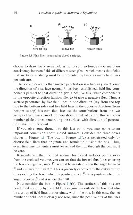
If you give some thought to this last point, you may come to an

important conclusion about closed surfaces. Consider the three boxes

shown in Figure 1.8. The box in Figure 1.8(a) is penetrated only by

electric field lines that originate and terminate outside the box. Thus,

every field line that enters must leave, and the flux through the box must

be zero.

Remembering that the unit normal for closed surfaces points away

from the enclosed volume, you can see that the inward flux (lines entering

the box) is negative, since ~E � n must be negative when the angle between

~E and n is greater than 90�. This is precisely cancelled by the outward flux

(lines exiting the box), which is positive, since ~E � n is positive when the

angle between ~E and n is less than 90�.Now consider the box in Figure 1.8(b). The surfaces of this box are

penetrated not only by the field lines originating outside the box, but also

by a group of field lines that originate within the box. In this case, the net

number of field lines is clearly not zero, since the positive flux of the lines

Zero net flux

(a) (b) (c)

Positive flux Negative flux

Figure 1.8 Flux lines penetrating closed surfaces.


that originate in the box is not compensated by any incoming (negative)

flux. Thus, you can say with certainty that if the flux through any closed

surface is positive, that surface must contain a source of field lines.

Finally, consider the box in Figure 1.8(c). In this case, some of the field

lines terminate within the box. These lines provide a negative flux at the

surface through which they enter, and since they don’t exit the box, their

contribution to the net flux is not compensated by any positive flux.

Clearly, if the flux through a closed surface is negative, that surface must

contain a sink of field lines (sometimes referred to as a drain).

Now recall the first rule of thumb for drawing charge-induced electric

field lines; they must originate on positive charge and terminate on

negative charge. So, the point from which the field lines diverge in Figure

1.8(b) marks the location of some amount of positive charge, and the

point to which the field lines converge in Figure 1.8(c) indicates the

existence of negative charge at that location.

If the amount of charge at these locations were greater, there would be

more field lines beginning or ending on these points, and the flux through

the surface would be greater. And if there were equal amounts of positive

and negative charge within one of these boxes, the positive (outward) flux

produced by the positive charge would exactly cancel the negative

(inward) flux produced by the negative charge. So, in this case the flux

would be zero, just as the net charge contained within the box would be

zero.

You should now see the physical reasoning behind Gauss’s law: the

electric flux passing through any closed surface – that is, the number of

electric field lines penetrating that surface – must be proportional to the

total charge contained within that surface. Before putting this concept to

use, you should take a look at the right side of Gauss’s law.


qenc The enclosed charge

If you understand the concept of flux as described in the previous section,

it should be clear why the right side of Gauss’s law involves only the

enclosed charge – that is, the charge within the closed surface over which

the flux is determined. Simply put, it is because any charge located out-

side the surface produces an equal amount of inward (negative) flux and

outward (positive) flux, so the net contribution to the flux through the

surface must be zero.

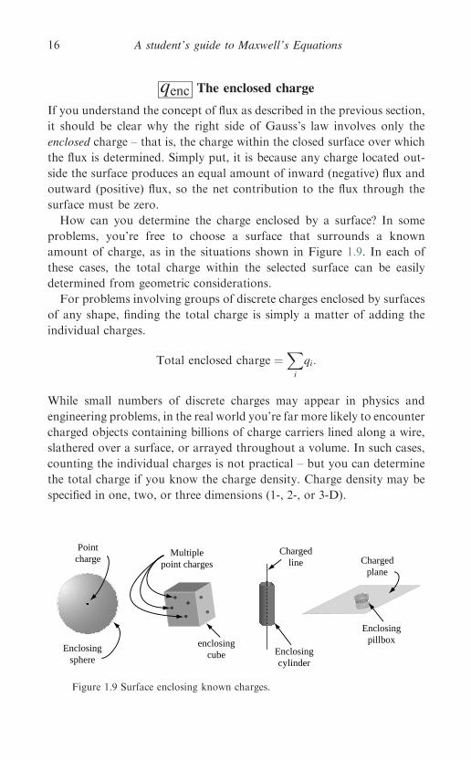
How can you determine the charge enclosed by a surface? In some

problems, you’re free to choose a surface that surrounds a known

amount of charge, as in the situations shown in Figure 1.9. In each of

these cases, the total charge within the selected surface can be easily

determined from geometric considerations.

For problems involving groups of discrete charges enclosed by surfaces

of any shape, finding the total charge is simply a matter of adding the

individual charges.

Total enclosed charge ¼Xi

qi:

While small numbers of discrete charges may appear in physics and

engineering problems, in the real world you’re far more likely to encounter

charged objects containing billions of charge carriers lined along a wire,

slathered over a surface, or arrayed throughout a volume. In such cases,

counting the individual charges is not practical – but you can determine

the total charge if you know the charge density. Charge density may be

specified in one, two, or three dimensions (1-, 2-, or 3-D).

Enclosingsphere

enclosingcube

Chargedline Charged

plane

Pointcharge

Multiplepoint charges

Enclosingcylinder

Enclosingpillbox

Figure 1.9 Surface enclosing known charges.


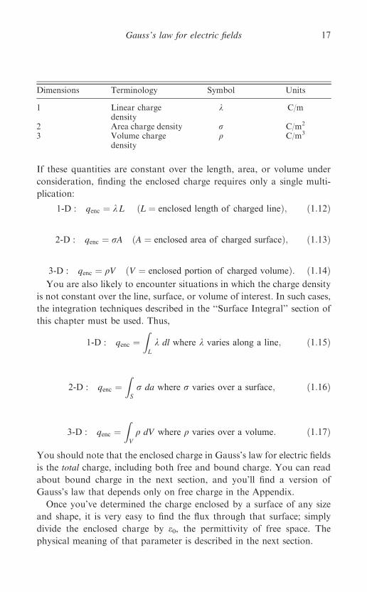
If these quantities are constant over the length, area, or volume under

consideration, finding the enclosed charge requires only a single multi-

plication:

1-D : qenc ¼ k L ðL ¼ enclosed length of charged lineÞ; ð1:12Þ

2-D : qenc ¼ rA ðA ¼ enclosed area of charged surfaceÞ; ð1:13Þ

3-D : qenc ¼ qV ðV ¼ enclosed portion of charged volumeÞ: ð1:14ÞYou are also likely to encounter situations in which the charge density

is not constant over the line, surface, or volume of interest. In such cases,

the integration techniques described in the ‘‘Surface Integral’’ section of

this chapter must be used. Thus,

1-D : qenc ¼ZL

k dl where k varies along a line; ð1:15Þ

2-D : qenc ¼ZS

r da where r varies over a surface; ð1:16Þ

3-D : qenc ¼ZV

q dV where q varies over a volume: ð1:17Þ

You should note that the enclosed charge in Gauss’s law for electric fields

is the total charge, including both free and bound charge. You can read

about bound charge in the next section, and you’ll find a version of

Gauss’s law that depends only on free charge in the Appendix.

Once you’ve determined the charge enclosed by a surface of any size

and shape, it is very easy to find the flux through that surface; simply

divide the enclosed charge by e0, the permittivity of free space. The

physical meaning of that parameter is described in the next section.

Dimensions Terminology Symbol Units

1 Linear chargedensity

k C/m

2 Area charge density r C/m2

3 Volume chargedensity

q C/m3


e0 The permittivity of free space

The constant of proportionality between the electric flux on the left side

of Gauss’s law and the enclosed charge on the right side is e0, the

permittivity of free space. The permittivity of a material determines

its response to an applied electric field – in nonconducting materials

(called ‘‘insulators’’ or ‘‘dielectrics’’), charges do not move freely, but

may be slightly displaced from their equilibrium positions. The relevant

permittivity in Gauss’s law for electric fields is the permittivity of free

space (or ‘‘vacuum permittivity’’), which is why it carries the subscript

zero.

The value of the vacuum permittivity in SI units is approximately

8.85 · 10�12 coulombs per volt-meter (C/Vm); you will sometimes see the

units of permittivity given as farads per meter (F/m), or, more funda-

mentally, (C2s2/kg m3). A more precise value for the permittivity of free

space is

e0¼ 8.8541878176 · 10�12 C/Vm.

Does the presence of this quantity mean that this form of Gauss’s law is

only valid in a vacuum? No, Gauss’s law as written in this chapter is

general, and applies to electric fields within dielectrics as well as those in

free space, provided that you account for all of the enclosed charge,

including charges that are bound to the atoms of the material.

The effect of bound charges can be understood by considering what

happens when a dielectric is placed in an external electric field. Inside the

dielectric material, the amplitude of the total electric field is generally less

than the amplitude of the applied field.

The reason for this is that dielectrics become ‘‘polarized’’ when placed

in an electric field, which means that positive and negative charges are

displaced from their original positions. And since positive charges are

displaced in one direction (parallel to the applied electric field) and

negative charges are displaced in the opposite direction (antiparallel to

the applied field), these displaced charges give rise to their own electric

field that opposes the external field, as shown in Figure 1.10. This makes

the net field within the dielectric less than the external field.

It is the ability of dielectric materials to reduce the amplitude of an

electric field that leads to their most common application: increasing the

capacitance and maximum operating voltage of capacitors. As you

may recall, the capacitance (ability to store charge) of a parallel-plate

capacitor is


C ¼ eAd;

where A is the plate area, d is the plate separation, and e is the permittivity

of the material between the plates. High-permittivity materials can

provide increased capacitance without requiring larger plate area or

decreased plate spacing.

The permittivity of a dielectric is often expressed as the relative per-

mittivity, which is the factor by which the material’s permittivity exceeds

that of free space:

relative permittivity er ¼ e=e0:

Some texts refer to relative permittivity as ‘‘dielectric constant,’’ although

the variation in permittivity with frequency suggests that the word ‘‘con-

stant’’ is better used elsewhere. The relative permittivity of ice, for example,

changes from approximately 81 at frequencies below 1kHz to less than 5 at

frequencies above 1MHz. Most often, it is the low-frequency value of

permittivity that is called the dielectric constant.

One more note about permittivity; as you’ll see in Chapter 5, the

permittivity of a medium is a fundamental parameter in determining the

speed with which an electromagnetic wave propagates through that

medium.

No dielectric present

Displacedcharges

Inducedfield

Dielectric

Externalelectric

field

+

+

+

+

–

–

–

–

Figure 1.10 Electric field induced in a dielectric.


Hs~E � n da ¼ qenc=e0 Applying Gauss’s law (integral form)

A good test of your understanding of an equation like Gauss’s law is

whether you’re able to solve problems by applying it to relevant situ-

ations. At this point, you should be convinced that Gauss’s law relates

the electric flux through a closed surface to the charge enclosed by that

surface. Here are some examples of what can you actually do with that

information.

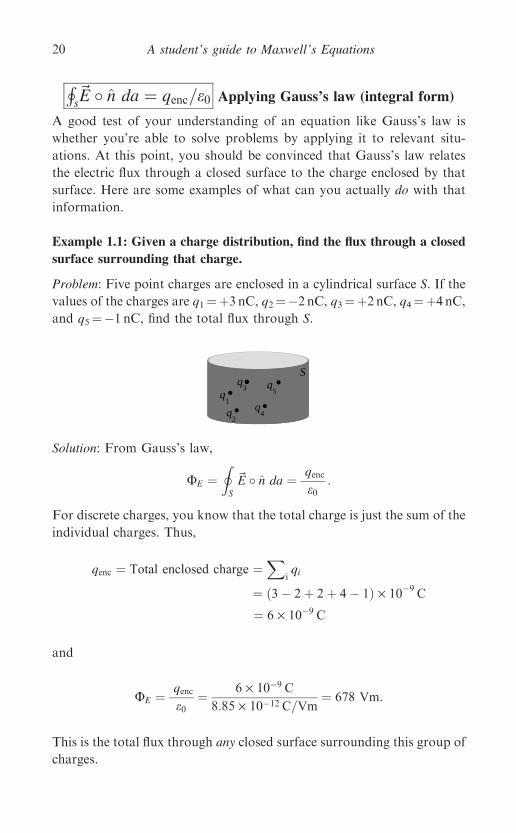
Example 1.1: Given a charge distribution, find the flux through a closed

surface surrounding that charge.

Problem: Five point charges are enclosed in a cylindrical surface S. If the

values of the charges are q1¼þ3 nC, q2¼�2 nC, q3¼þ2 nC, q4¼þ4 nC,

and q5¼�1 nC, find the total flux through S.

Solution: From Gauss’s law,

UE ¼IS

~E � n da ¼ qenc

e0:

For discrete charges, you know that the total charge is just the sum of the

individual charges. Thus,

qenc ¼ Total enclosed charge ¼X

iqi

¼ ð3� 2þ 2þ 4� 1Þ · 10�9

C

¼ 6 · 10�9 C

and

UE ¼ qenc

e0¼ 6 · 10�9 C

8:85 · 10�12 C=Vm¼ 678 Vm:

This is the total flux through any closed surface surrounding this group of

charges.

S

q1

q3

q2

q5

q4


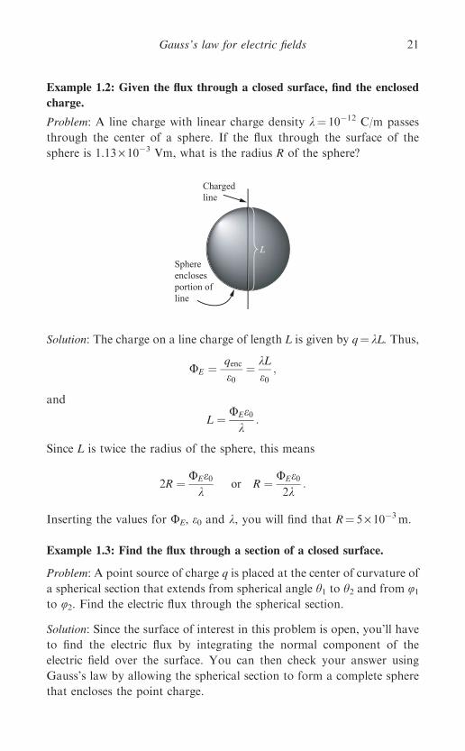
Example 1.2: Given the flux through a closed surface, find the enclosed

charge.

Problem: A line charge with linear charge density k¼ 10�12 C/m passes

through the center of a sphere. If the flux through the surface of the

sphere is 1.13 · 10�3 Vm, what is the radius R of the sphere?

Solution: The charge on a line charge of length L is given by q¼ kL. Thus,

UE ¼ qenc

e0¼ kL

e0;

and

L ¼ UEe0k

:

Since L is twice the radius of the sphere, this means

2R ¼ UEe0k

or R ¼ UEe02k

:

Inserting the values for UE, e0 and k, you will find that R¼ 5 · 10�3m.

Example 1.3: Find the flux through a section of a closed surface.

Problem: A point source of charge q is placed at the center of curvature of

a spherical section that extends from spherical angle h1 to h2 and from u1to u2. Find the electric flux through the spherical section.

Solution: Since the surface of interest in this problem is open, you’ll have

to find the electric flux by integrating the normal component of the

electric field over the surface. You can then check your answer using

Gauss’s law by allowing the spherical section to form a complete sphere

that encloses the point charge.

Chargedline

L

Sphereenclosesportion ofline


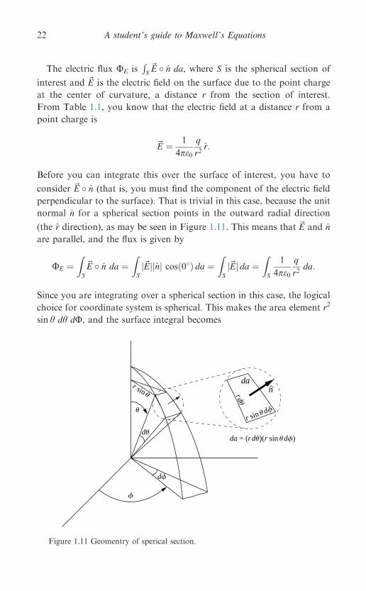
The electric flux UE isRS~E � n da, where S is the spherical section of

interest and ~E is the electric field on the surface due to the point charge

at the center of curvature, a distance r from the section of interest.

From Table 1.1, you know that the electric field at a distance r from a

point charge is

~E ¼ 1

4pe0

q

r2r:

Before you can integrate this over the surface of interest, you have to

consider ~E � n (that is, you must find the component of the electric field

perpendicular to the surface). That is trivial in this case, because the unit

normal n for a spherical section points in the outward radial direction

(the r direction), as may be seen in Figure 1.11. This means that ~E and n

are parallel, and the flux is given by

UE ¼ZS

~E � n da ¼ZS

j~Ejjnj cosð0�Þ da ¼ZS

j~Ej da ¼ZS

1

4pe0

q

r2da:

Since you are integrating over a spherical section in this case, the logical

choice for coordinate system is spherical. This makes the area element r2

sin h dh dU, and the surface integral becomes

rdu

r sin udf

dan

df

du

f

r sin u

u

da = (rdu)(r sin udf)

Figure 1.11 Geomentry of sperical section.


UE ¼Zh

Zf

1

4pe0

q

r2r2 sin h dh df ¼ q

4pe0

Zhsin h dh

Zfdf;

which is easily integrated to give

UE ¼ q

4pe0ðcos h1 � cos h2Þðf2 � f1Þ:

As a check on this result, take the entire sphere as the section (h1¼ 0,

h2¼ p, u1¼ 0, and u2¼ 2p). This gives

UE ¼ q

4pe0ð1� ð�1ÞÞ ð2p� 0Þ ¼ q

e0;

exactly as predicted by Gauss’s law.

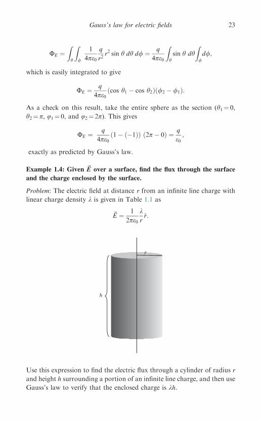
Example 1.4: Given ~E over a surface, find the flux through the surface

and the charge enclosed by the surface.

Problem: The electric field at distance r from an infinite line charge with

linear charge density k is given in Table 1.1 as

~E ¼ 1

2pe0

krr:

Use this expression to find the electric flux through a cylinder of radius r

and height h surrounding a portion of an infinite line charge, and then use

Gauss’s law to verify that the enclosed charge is kh.

h

r


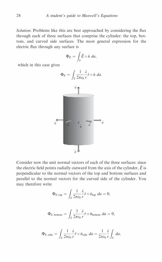
Solution: Problems like this are best approached by considering the flux

through each of three surfaces that comprise the cylinder: the top, bot-

tom, and curved side surfaces. The most general expression for the

electric flux through any surface is

UE ¼ZS

~E � n da;

which in this case gives

UE ¼ZS

1

2pe0

krr � n da:

Consider now the unit normal vectors of each of the three surfaces: since

the electric field points radially outward from the axis of the cylinder, ~E is

perpendicular to the normal vectors of the top and bottom surfaces and

parallel to the normal vectors for the curved side of the cylinder. You

may therefore write

UE; top ¼ZS

1

2pe0

krr � ntop da ¼ 0;

UE; bottom ¼ZS

1

2pe0

krr � nbottom da ¼ 0;

UE; side ¼ZS

1

2pe0

krr � nside da ¼ 1

2pe0

kr

ZS

da;

n

nn

n

n nn


and, since the area of the curved side of the cylinder is 2prh, this gives

UE;side ¼ 1

2pe0

krð2prhÞ ¼ kh

e0:

Gauss’s law tells you that this must equal qenc /e0, which verifies that the

enclosed charge qenc¼ kh in this case.

Example 1.5: Given a symmetric charge distribution, find ~E:

Finding the electric field using Gauss’s law may seem to be a hopeless

task. After all, while the electric field does appear in the equation, it is only

the normal component that emerges from the dot product, and it is only

the integral of that normal component over the entire surface that is propo-

rtional to the enclosed charge. Do realistic situations exist in which it is

possible to dig the electric field out of its interior position in Gauss’s law?

Happily, the answer is yes; you may indeed find the electric field

using Gauss’s law, albeit only in situations characterized by high sym-

metry. Specifically, you can determine the electric field whenever you’re

able to design a real or imaginary ‘‘special Gaussian surface’’ that

encloses a known amount of charge. A special Gaussian surface is one on

which

(1) the electric field is either parallel or perpendicular to the surface

normal (which allows you to convert the dot product into an

algebraic multiplication), and

(2) the electric field is constant or zero over sections of the surface (which

allows you to remove the electric field from the integral).

Of course, the electric field on any surface that you can imagine around

arbitrarily shaped charge distributions will not satisfy either of these

requirements. But there are situations in which the distribution of charge

is sufficiently symmetric that a special Gaussian surface may be imagined.

Specifically, the electric field in the vicinity of spherical charge distribu-

tions, infinite lines of charge, and infinite planes of charge may be

determined by direct application of the integral form of Gauss’s law.

Geometries that approximate these ideal conditions, or can be approxi-

mated by combinations of them, may also be attacked using Gauss’s law.

The following problem shows how to use Gauss’s law to find the

electric field around a spherical distribution of charge; the other cases are

covered in the problem set, for which solutions are available on the

website.


Problem: Use Gauss’s law to find the electric field at a distance r from the

center of a sphere with uniform volume charge density q and radius a.

Solution: Consider first the electric field outside the sphere. Since the

distribution of charge is spherically symmetric, it is reasonable to expect

the electric field to be entirely radial (that is, pointed toward or away

from the sphere). If that’s not obvious to you, imagine what would

happen if the electric field had a nonradial component (say in the h or ’

direction); by rotating the sphere about some arbitrary axis, you’d be able

to change the direction of the field. But the charge is uniformly distrib-

uted throughout the sphere, so there can be no preferred direction or

orientation – rotating the sphere simply replaces one chunk of charge

with another, identical chunk – so this can have no effect whatsoever on

the electric field. Faced with this conundrum, you are forced to conclude

that the electric field of a spherically symmetric charge distribution must

be entirely radial.

To find the value of this radial field using Gauss’s law, you’ll have to

imagine a surface that meets the requirements of a special Gaussian

surface; ~E must be either parallel or perpendicular to the surface normal

at all locations, and ~E must be uniform everywhere on the surface. For a

radial electric field, there can be only one choice; your Gaussian surface

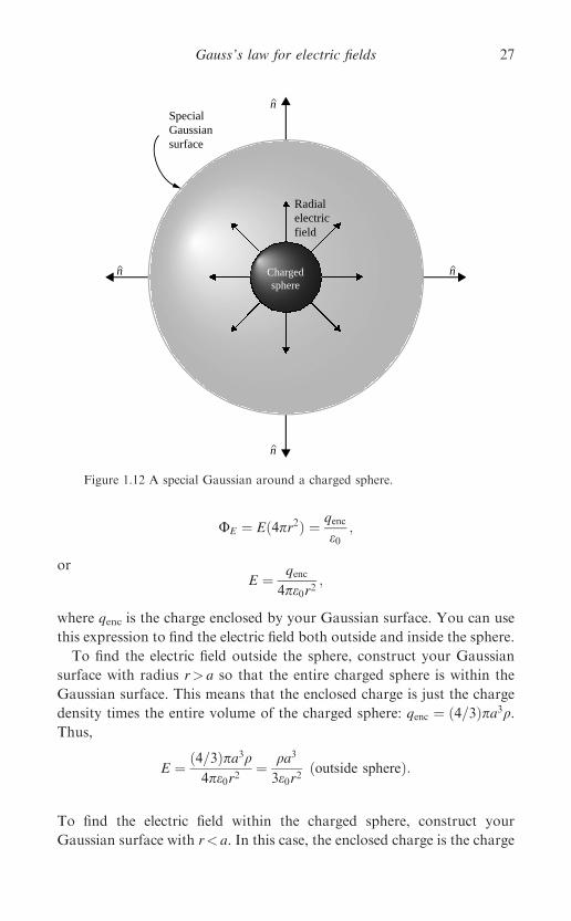
must be a sphere centered on the charged sphere, as shown in Figure 1.12.

Notice that no actual surface need be present, and the special Gaussian

surface may be purely imaginary – it is simply a construct that allows you

to evaluate the dot product and remove the electric field from the surface

integral in Gauss’s law.

Since the radial electric field is everywhere parallel to the surface

normal, the ~E � n term in the integral in Gauss’s law becomes

j~Ejjnj cosð0�Þ, and the electric flux over the Gaussian surface S is

UE ¼IS

~E � n da ¼IS

E da

Since ~E has no h or u dependence, it must be constant over S, which

means it may be removed from the integral:

UE ¼IS

E da ¼ E

IS

da ¼ Eð4pr2Þ;

where r is the radius of the special Gaussian surface. You can now use

Gauss’s law to find the value of the electric field:


UE ¼ Eð4pr2Þ ¼ qenc

e0;

orE ¼ qenc

4pe0r2;

where qenc is the charge enclosed by your Gaussian surface. You can use

this expression to find the electric field both outside and inside the sphere.

To find the electric field outside the sphere, construct your Gaussian

surface with radius r> a so that the entire charged sphere is within the

Gaussian surface. This means that the enclosed charge is just the charge

density times the entire volume of the charged sphere: qenc ¼ ð4=3Þpa3q.Thus,

E ¼ ð4=3Þpa3q4pe0r2

¼ qa3

3e0r2ðoutside sphereÞ:

To find the electric field within the charged sphere, construct your

Gaussian surface with r< a. In this case, the enclosed charge is the charge

Radialelectricfield

Chargedsphere

nSpecialGaussiansurface

n

nn

Figure 1.12 A special Gaussian around a charged sphere.


density times the volume of your Gaussian surface: qenc ¼ ð4=3Þpr3q.Thus,

E ¼ ð4=3Þpr3q4pe0r2

¼ qr3e0

ðinside sphereÞ:

The keys to successfully employing special Gaussian surfaces are to

recognize the appropriate shape for the surface and then to adjust its size

to ensure that it runs through the point at which you wish to determine

the electric field.


1.2 The differential form of Gauss’s law

The integral form of Gauss’s law for electric fields relates the electric flux

over a surface to the charge enclosed by that surface – but like all of

Maxwell’s Equations, Gauss’s law may also be cast in differential form.

The differential form is generally written as

~r �~E ¼ qe0

Gauss’s law for electric fields ðdifferential formÞ:

The left side of this equation is a mathematical description of the

divergence of the electric field – the tendency of the field to ‘‘flow’’ away

from a specified location – and the right side is the electric charge density

divided by the permittivity of free space.

Don’t be concerned if the del operator (~r) or the concept of divergence

isn’t perfectly clear to you – these are discussed in the following sections.

For now, make sure you grasp the main idea of Gauss’s law in differential

form:

The electric field produced by electric charge diverges from positive

charge and converges upon negative charge.

In other words, the only places at which the divergence of the electric field

is not zero are those locations at which charge is present. If positive

charge is present, the divergence is positive, meaning that the electric field

tends to ‘‘flow’’ away from that location. If negative charge is present, the

divergence is negative, and the field lines tend to ‘‘flow’’ toward that

point.

Note that there’s a fundamental difference between the differential

and the integral form of Gauss’s law; the differential form deals with the

divergence of the electric field and the charge density at individual points

in space, whereas the integral form entails the integral of the normal

component of the electric field over a surface. Familiarity with both forms

will allow you to use whichever is better suited to the problem you’re

trying to solve.


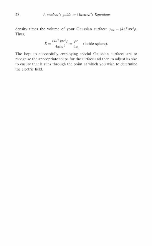
To help you understand the meaning of each symbol in the differential

form of Gauss’s law for electric fields, here’s an expanded view:

How is the differential form of Gauss’s law useful? In any problem in

which the spatial variation of the vector electric field is known at a

specified location, you can find the volume charge density at that location

using this form. And if the volume charge density is known, the

divergence of the electric field may be determined.

E� �0= �

Reminder that del isa vector operator

Reminder that the electricfield is a vector

The differentialoperator called “del” or “nabla”

The dot product turnsthe del operator into the divergence

The electricfield in N/C

The electricpermittivity offree space

The charge density in coulombs per cubic meter


~r Nabla – the del operator

An inverted uppercase delta appears in the differential form of all four of

Maxwell’s Equations. This symbol represents a vector differential operator

called ‘‘nabla’’ or ‘‘del,’’ and its presence instructs you to take derivatives

of the quantity on which the operator is acting. The exact form of those

derivatives depends on the symbol following the del operator, with ‘‘~r�’’signifying divergence, ‘‘~r ·’’ indicating curl, and ~r signifying gradient.

Each of these operations is discussed in later sections; for now we’ll just

consider what an operator is and how the del operator can be written in

Cartesian coordinates.

Like all good mathematical operators, del is an action waiting to

happen. Just as H tells you to take the square root of anything that

appears under its roof, ~r is an instruction to take derivatives in three

directions. Specifically,

~r � i@

@xþ j

@

@yþ k

@

@z; ð1:18Þ

where i, j, and k are the unit vectors in the direction of the Cartesian

coordinates x, y, and z. This expression may appear strange, since in this

form it is lacking anything on which it can operate. In Gauss’s law for

electric fields, the del operator is dotted into the electric field vector,

forming the divergence of ~E. That operation and its results are described

in the next section.


~r� Del dot – the divergence

The concept of divergence is important in many areas of physics and

engineering, especially those concerned with the behavior of vector fields.

James Clerk Maxwell coined the term ‘‘convergence’’ to describe the

mathematical operation that measures the rate at which electric field lines

‘‘flow’’ toward points of negative electric charge (meaning that positive

convergence was associated with negative charge). A few years later,

Oliver Heaviside suggested the use of the term ‘‘divergence’’ for the same

quantity with the opposite sign. Thus, positive divergence is associated

with the ‘‘flow’’ of electric field lines away from positive charge.

Both flux and divergence deal with the ‘‘flow’’ of a vector field, but

with an important difference; flux is defined over an area, while diver-

gence applies to individual points. In the case of fluid flow, the divergence

at any point is a measure of the tendency of the flow vectors to diverge

from that point (that is, to carry more material away from it than is

brought toward it). Thus points of positive divergence are sources (fau-

cets in situations involving fluid flow, positive electric charge in electro-

statics), while points of negative divergence are sinks (drains in fluid flow,

negative charge in electrostatics).

The mathematical definition of divergence may be understood by

considering the flux through an infinitesimal surface surrounding the

point of interest. If you were to form the ratio of the flux of a vector field

~A through a surface S to the volume enclosed by that surface as the

volume shrinks toward zero, you would have the divergence of ~A:

divð~AÞ ¼ ~r �~A � limDV!0

1

DV

IS

~A � n da: ð1:19Þ

While this expression states the relationship between divergence and flux,

it is not particularly useful for finding the divergence of a given vector

field. You’ll find a more user-friendly mathematical expression for

divergence later in this section, but first you should take a look at the

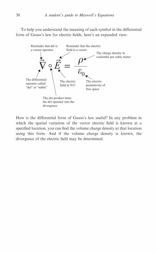
vector fields shown in Figure 1.13.

To find the locations of positive divergence in each of these fields, look

for points at which the flow vectors either spread out or are larger

pointing away from the location and shorter pointing toward it. Some

authors suggest that you imagine sprinkling sawdust on flowing water to

assess the divergence; if the sawdust is dispersed, you have selected a

point of positive divergence, while if it becomes more concentrated,

you’ve picked a location of negative divergence.


Using such tests, it is clear that locations such as 1 and 2 in Figure 1.13(a)

and location 3 in Figure 1.13(b) are points of positive divergence, while

the divergence is negative at point 4.

The divergence at various points in Figure 1.13(c) is less obvious.

Location 5 is obviously a point of positive divergence, but what about

locations 6 and 7? The flow lines are clearly spreading out at those loca-

tions, but they’re also getting shorter at greater distance from the center.

Does the spreading out compensate for the slowing down of the flow?

Answering that question requires a useful mathematical form of the

divergence as well as a description of how the vector field varies from

place to place. The differential form of the mathematical operation of

divergence or ‘‘del dot’’ (~r�) on a vector ~A in Cartesian coordinates is

~r �~A ¼ i@

@xþ j

@

@yþ k

@

@z

� �� iAx þ jAy þ kAz

� �;

and, since i � i ¼ j � j ¼ k � k ¼ 1; this is

~r �~A ¼ @Ax

@xþ @Ay

@yþ @Az

@z

� �: ð1:20Þ

Thus, the divergence of the vector field ~A is simply the change in its

x-component along the x-axis plus the change in its y-component along

the y-axis plus the change in its z-component along the z-axis. Note that

the divergence of a vector field is a scalar quantity; it has magnitude but

no direction.

1

4

3 5

2

6

7

(a) (b) (c)

Figure 1.13 Vector fields with various values of divergence.


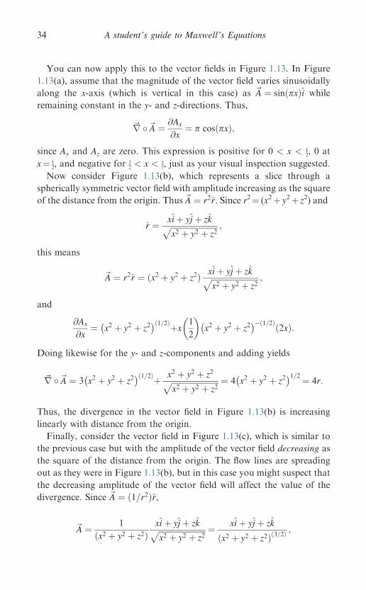
You can now apply this to the vector fields in Figure 1.13. In Figure

1.13(a), assume that the magnitude of the vector field varies sinusoidally

along the x-axis (which is vertical in this case) as ~A ¼ sinðpxÞi while

remaining constant in the y- and z-directions. Thus,

~r �~A ¼ @Ax

@x¼ p cosðpxÞ;

since Ay and Az are zero. This expression is positive for 0 < x < 12, 0 at

x¼ 12, and negative for 1

2 < x < 32, just as your visual inspection suggested.

Now consider Figure 1.13(b), which represents a slice through a

spherically symmetric vector field with amplitude increasing as the square

of the distance from the origin. Thus~A ¼ r2r. Since r2¼ (x2þ y2þ z2) and

r ¼ xiþ yjþ zkffiffiffiffiffiffiffiffiffiffiffiffiffiffiffiffiffiffiffiffiffiffiffiffix2 þ y2 þ z2

p ;

this means

~A ¼ r2r ¼ ðx2 þ y2 þ z2Þ xiþ yjþ zkffiffiffiffiffiffiffiffiffiffiffiffiffiffiffiffiffiffiffiffiffiffiffiffix2 þ y2 þ z2

p ;

and

@Ax

@x¼ x2 þ y2 þ z2� �ð1=2Þþx

1

2

� �x2 þ y2 þ z2� ��ð1=2Þ

2xð Þ:

Doing likewise for the y- and z-components and adding yields

~r �~A ¼ 3 x2 þ y2 þ z2� �ð1=2Þþ x2 þ y2 þ z2ffiffiffiffiffiffiffiffiffiffiffiffiffiffiffiffiffiffiffiffiffiffiffiffi

x2 þ y2 þ z2p ¼ 4 x2 þ y2 þ z2

� �1=2 ¼ 4r:

Thus, the divergence in the vector field in Figure 1.13(b) is increasing

linearly with distance from the origin.

Finally, consider the vector field in Figure 1.13(c), which is similar to

the previous case but with the amplitude of the vector field decreasing as

the square of the distance from the origin. The flow lines are spreading

out as they were in Figure 1.13(b), but in this case you might suspect that

the decreasing amplitude of the vector field will affect the value of the

divergence. Since ~A ¼ ð1=r2Þr,

~A ¼ 1

x2 þ y2 þ z2ð Þxiþ yjþ zkffiffiffiffiffiffiffiffiffiffiffiffiffiffiffiffiffiffiffiffiffiffiffiffix2 þ y2 þ z2

p ¼ xiþ yjþ zk

x2 þ y2 þ z2ð Þð3=2Þ;


and

@Ax

@x¼ 1

x2 þ y2 þ z2ð Þð3=2Þ– x

3

2

� �x2 þ y2 þ z2� ��ð5=2Þ

2xð Þ;

Adding in the y- and z-derivatives gives

~r �~A ¼ 3

x2 þ y2 þ z2ð Þð3=2Þ� 3 x2 þ y2 þ z2

� �x2 þ y2 þ z2ð Þð5=2Þ

¼ 0:

This validates the suspicion that the reduced amplitude of the vector field

with distance from the origin may compensate for the spreading out of

the flow lines. Note that this is true only for the case in which the

amplitude of the vector field falls off as 1/r2 (this case is especially rele-

vant for the electric field, which you’ll find in the next section).

As you consider the divergence of the electric field, you should

remember that some problems may be solved more easily using non-

Cartesian coordinate systems. The divergence may be calculated in

cylindrical and spherical coordinate systems using

~r �~A ¼ 1

r

@

@rðrArÞ þ 1

r

@Af

@fþ @Az

@zðcylindricalÞ; ð1:21Þ

and

~r �~A ¼ 1

r2@

@rðr2ArÞ þ 1

r sin h@

@hðAh sin hÞ

þ 1

r sin h

@Af

@fðsphericalÞ:

ð1:22Þ

If you doubt the efficacy of choosing the proper coordinate system, you

should rework the last two examples in this section using spherical

coordinates.


~r �~E The divergence of the electric field

This expression is the entire left side of the differential form of Gauss’s

law, and it represents the divergence of the electric field. In electrostatics,

all electric field lines begin on points of positive charge and terminate

on points of negative charge, so it is understandable that this expression

is proportional to the electric charge density at the location under

consideration.

Consider the electric field of the positive point charge; the electric field

lines originate on the positive charge, and you know from Table 1.1 that

the electric field is radial and decreases as 1/r2:

~E ¼ 1

4pe0

q

r2r:

This is analogous to the vector field shown in Figure 1.13(c), for which

the divergence is zero. Thus, the spreading out of the electric field lines is

exactly compensated by the 1/r2 reduction in field amplitude, and the

divergence of the electric field is zero at all points away from the origin.

The reason the origin (where r¼ 0) is not included in the previous

analysis is that the expression for the divergence includes terms con-

taining r in the denominator, and those terms become problematic as r

approaches zero. To evaluate the divergence at the origin, use the formal

definition of divergence:

~r �~E � limDV!0

1

DV

IS

~E � n da:

Considering a special Gaussian surface surrounding the point charge

q, this is

~r �~E � limDV!0

1

DV

q

4pe0r2

IS

da

0@

1A ¼ lim

DV!0

1

DV

q

4pe0r2ð4pr2Þ

� �

¼ limDV!0

1

DV

q

e0

� �:

But q/DV is just the average charge density over the volume DV, and as

DV shrinks to zero, this becomes equal to q, the charge density at the

origin. Thus, at the origin the divergence is

~r �~E ¼ qe0;

in accordance with Gauss’s law.


It is worth your time to make sure you understand the significance of

this last point. A casual glance at the electric field lines in the vicinity of a

point charge suggests that they ‘‘diverge’’ everywhere (in the sense of

getting farther apart). But as you’ve seen, radial vector fields that

decrease in amplitude as 1/r2 actually have zero divergence everywhere

except at the source. The key factor in determining the divergence at any

point is not simply the spacing of the field lines at that point, but whether

the flux out of an infinitesimally small volume around the point is greater

than, equal to, or less than the flux into that volume. If the outward flux

exceeds the inward flux, the divergence is positive at that point. If the

outward flux is less than the inward flux, the divergence is negative, and if

the outward and inward fluxes are equal the divergence is zero at that

point.

In the case of a point charge at the origin, the flux through an infini-

tesimally small surface is nonzero only if that surface contains the point

charge. Everywhere else, the flux into and out of that tiny surface must be

the same (since it contains no charge), and the divergence of the electric

field must be zero.


~r �~E ¼ q=e0 Applying Gauss’s law (differential form)

The problems you’re most likely to encounter that can be solved using the

differential form of Gauss’s law involve calculating the divergence of the

electric field and using the result to determine the charge density at a

specified location.

The following examples should help you understand how to solve

problems of this type.

Example 1.6: Given an expression for the vector electric field, find the

divergence of the field at a specified location.

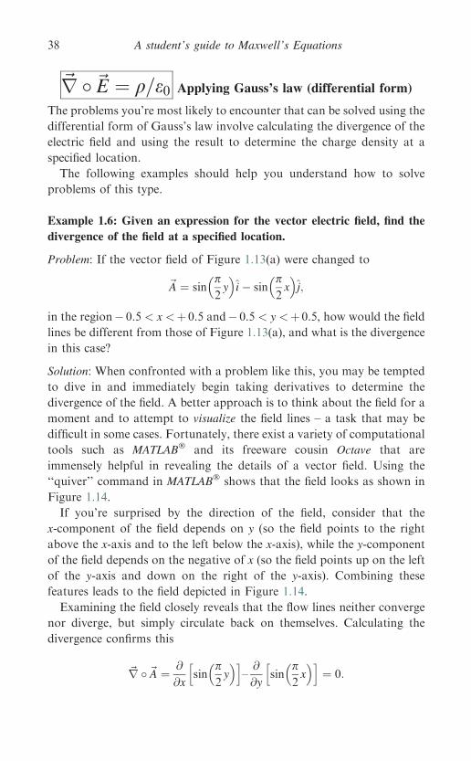
Problem: If the vector field of Figure 1.13(a) were changed to

~A ¼ sinp2y

� �i� sin

p2x

� �j;

in the region� 0.5 < x <þ 0.5 and� 0.5 < y <þ 0.5, how would the field

lines be different from those of Figure 1.13(a), and what is the divergence

in this case?

Solution: When confronted with a problem like this, you may be tempted

to dive in and immediately begin taking derivatives to determine the

divergence of the field. A better approach is to think about the field for a

moment and to attempt to visualize the field lines – a task that may be

difficult in some cases. Fortunately, there exist a variety of computational

tools such as MATLAB� and its freeware cousin Octave that are

immensely helpful in revealing the details of a vector field. Using the

‘‘quiver’’ command in MATLAB� shows that the field looks as shown in

Figure 1.14.

If you’re surprised by the direction of the field, consider that the

x-component of the field depends on y (so the field points to the right

above the x-axis and to the left below the x-axis), while the y-component

of the field depends on the negative of x (so the field points up on the left

of the y-axis and down on the right of the y-axis). Combining these

features leads to the field depicted in Figure 1.14.

Examining the field closely reveals that the flow lines neither converge

nor diverge, but simply circulate back on themselves. Calculating the

divergence confirms this

~r �~A ¼ @

@xsin

p2y

� �h i–@

@ysin

p2x

� �h i¼ 0:


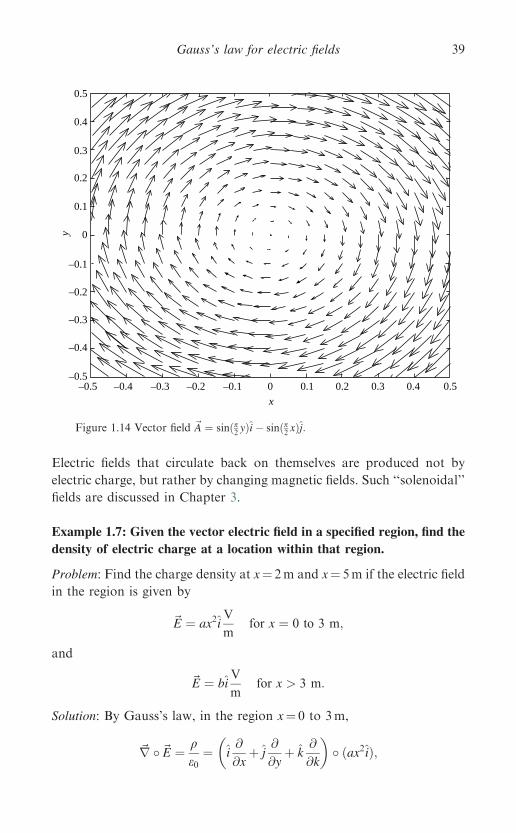
Electric fields that circulate back on themselves are produced not by

electric charge, but rather by changing magnetic fields. Such ‘‘solenoidal’’

fields are discussed in Chapter 3.

Example 1.7: Given the vector electric field in a specified region, find the

density of electric charge at a location within that region.

Problem: Find the charge density at x¼ 2m and x¼ 5m if the electric field

in the region is given by

~E ¼ ax2iV

mfor x ¼ 0 to 3 m;

and

~E ¼ biV

mfor x > 3 m:

Solution: By Gauss’s law, in the region x¼ 0 to 3m,

~r �~E ¼ qe0

¼ i@

@xþ j

@

@yþ k

@

@k

� �� ðax2iÞ;

0.5

0.4

0.3

0.2

0.1

0

–0.1

–0.1

–0.2

–0.2

–0.3

–0.3

–0.4

–0.4–0.5

–0.5 0 0.1 0.2 0.3 0.4 0.5

y

x

Figure 1.14 Vector field ~A ¼ sinðp2 yÞi� sinðp2 xÞj:


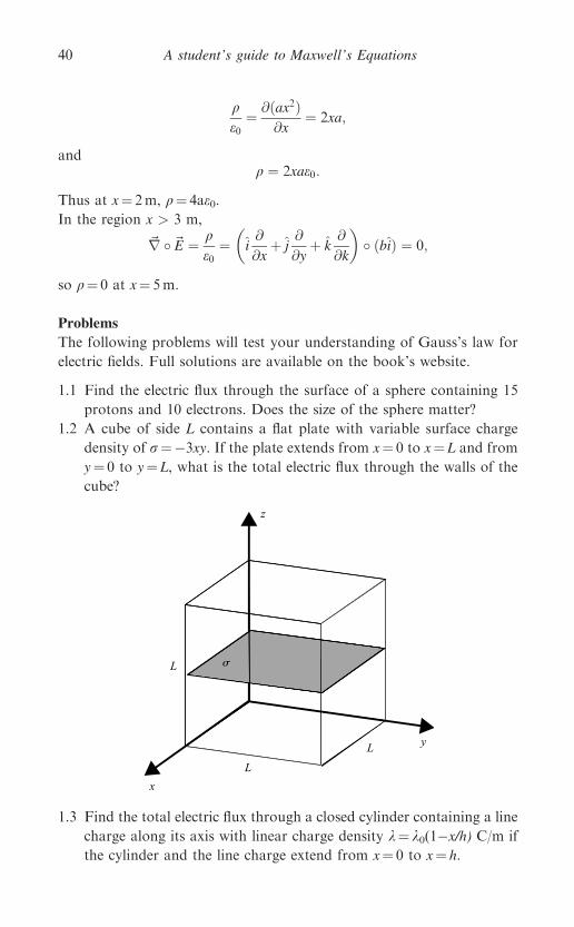
qe0

¼ @ðax2Þ@x

¼ 2xa;

andq ¼ 2xae0:

Thus at x¼ 2m, q¼ 4ae0.In the region x > 3 m,

~r �~E ¼ qe0

¼ i@

@xþ j

@

@yþ k

@

@k

� �� ðbiÞ ¼ 0;

so q¼ 0 at x¼ 5m.

Problems

The following problems will test your understanding of Gauss’s law for

electric fields. Full solutions are available on the book’s website.

1.1 Find the electric flux through the surface of a sphere containing 15

protons and 10 electrons. Does the size of the sphere matter?

1.2 A cube of side L contains a flat plate with variable surface charge

density of r¼�3xy. If the plate extends from x¼ 0 to x¼ L and from

y¼ 0 to y¼ L, what is the total electric flux through the walls of the

cube?

1.3 Find the total electric flux through a closed cylinder containing a line

charge along its axis with linear charge density k¼ k0(1�x/h) C/m if

the cylinder and the line charge extend from x¼ 0 to x¼ h.

s

x

y

z

L

L

L


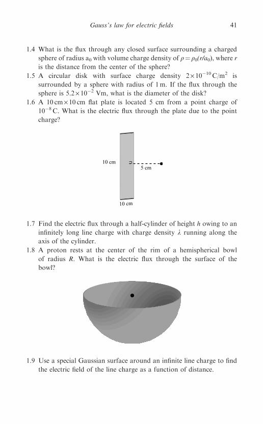
1.4 What is the flux through any closed surface surrounding a charged

sphere of radius a0 with volume charge density of q¼ q0(r/a0), where ris the distance from the center of the sphere?

1.5 A circular disk with surface charge density 2 · 10�10 C/m2 is

surrounded by a sphere with radius of 1m. If the flux through the

sphere is 5.2 · 10�2 Vm, what is the diameter of the disk?

1.6 A 10 cm · 10 cm flat plate is located 5 cm from a point charge of

10�8 C. What is the electric flux through the plate due to the point

charge?

1.7 Find the electric flux through a half-cylinder of height h owing to an

infinitely long line charge with charge density k running along the

axis of the cylinder.

1.8 A proton rests at the center of the rim of a hemispherical bowl

of radius R. What is the electric flux through the surface of the

bowl?

1.9 Use a special Gaussian surface around an infinite line charge to find

the electric field of the line charge as a function of distance.

10 cm

10 cm5 cm


1.10 Use a special Gaussian surface to prove that the magnitude of the

electric field of an infinite flat plane with surface charge density r is

j~Ej ¼ r=2e0.1.11 Find the divergence of the field given by ~A ¼ ð1=rÞr in spherical

coordinates.

1.12 Find the divergence of the field given by ~A ¼ rr in spherical

coordinates.

1.13 Given the vector field

~A ¼ cos py –p2

� �iþ sin pxð Þj;

sketch the field lines and find the divergence of the field.

1.14 Find the charge density in a region for which the electric field in

cylindrical coordinates is given by

~E ¼ az

rr þ brfþ cr2z2z

1.15 Find the charge density in a region for which the electric field in

spherical coordinates is given by

~E ¼ ar2r þ b cos ðhÞr

hþ cf:


2

Gauss’s law for magnetic fields

Gauss’s law for magnetic fields is similar in form but different in content

from Gauss’s law for electric fields. For both electric and magnetic fields,

the integral form of Gauss’s law involves the flux of the field over a closed

surface, and the differential form specifies the divergence of the field at a

point.

The key difference in the electric field and magnetic field versions of

Gauss’s law arises because opposite electric charges (called ‘‘positive’’

and ‘‘negative’’) may be isolated from one another, while opposite

magnetic poles (called ‘‘north’’ and ‘‘south’’) always occur in pairs. As

you might expect, the apparent lack of isolated magnetic poles in nature

has a profound impact on the behavior of magnetic flux and on the

divergence of the magnetic field.

2.1 The integral form of Gauss’s law

Notation differs among textbooks, but the integral form of Gauss’s law is

generally written as follows:IS

~B � n da ¼ 0 Gauss’s law for magnetic fields ðintegral formÞ:

As de scribed in the prev ious chapter , the left side of this equati on is a

mathematical description of the flux of a vector field through a closed

surface. In this case, Gauss’s law refers to magnetic flux – the number of

magnetic field lines – passing through a closed surface S. The right side is

identically zero.

In this chapter, you will see why this law is different from the electric

field case, and you will find some examples of how to use the magnetic

43

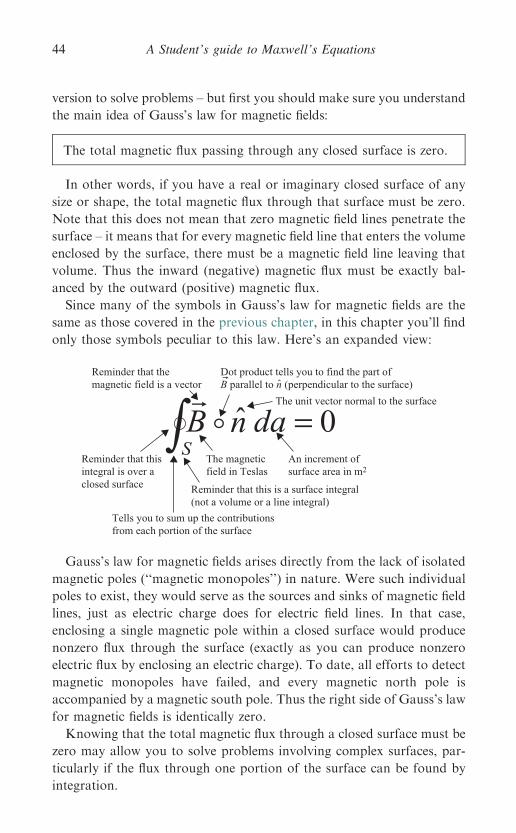
ˆ =S

da 0nBReminder that thisintegral is over aclosed surface

The magneticfield in Teslas

Reminder that the magnetic field is a vector ˆ

Dot product tells you to find the part of B parallel to n (perpendicular to the surface)

The unit vector normal to the surface

Reminder that this is a surface integral (not a volume or a line integral)

An increment ofsurface area in m2

Tells you to sum up the contributions from each portion of the surface

∫

version to solve problems – but first you should make sure you understand

the main idea of Gauss’s law for magnetic fields:

The total magnetic flux passing through any closed surface is zero.

In other words, if you have a real or imaginary closed surface of any

size or shape, the total magnetic flux through that surface must be zero.

Note that this does not mean that zero magnetic field lines penetrate the

surface – it means that for every magnetic field line that enters the volume

enclosed by the surface, there must be a magnetic field line leaving that

volume. Thus the inward (negative) magnetic flux must be exactly bal-

anced by the outward (positive) magnetic flux.

Since many of the symbols in Gauss’s law for magnetic fields are the

same as those covered in the pre vious chap ter, in this ch apter you ’ll find

only those symbols peculiar to this law. Here’s an expanded view:

Gauss’s law for magnetic fields arises directly from the lack of isolated

magnetic poles (‘‘magnetic monopoles’’) in nature. Were such individual

poles to exist, they would serve as the sources and sinks of magnetic field

lines, just as electric charge does for electric field lines. In that case,

enclosing a single magnetic pole within a closed surface would produce

nonzero flux through the surface (exactly as you can produce nonzero

electric flux by enclosing an electric charge). To date, all efforts to detect

magnetic monopoles have failed, and every magnetic north pole is

accompanied by a magnetic south pole. Thus the right side of Gauss’s law

for magnetic fields is identically zero.

Knowing that the total magnetic flux through a closed surface must be

zero may allow you to solve problems involving complex surfaces, par-

ticularly if the flux through one portion of the surface can be found by

integration.

A Student’s guide to Maxwell’s Equations44

~B The magnetic field

Just as the electric field may be defined by considering the electric force

on a small test charge, the magnetic field may be defined using the

magnetic force experienced by a moving charged particle. As you may

recall, charged particles experience magnetic force only if they are in

motion with respect to the magnetic field, as shown by the Lorentz

equation for magnetic force:

~FB ¼ q~v ·~B ð2:1Þwhere ~FB is the magnetic force, q is the particle’s charge,~v is the particle’s

velocity (with respect to ~B), and ~B is the magnetic field.

Using the definition of the vector cross-product which says that

~a ·~b ¼ j~ajj~bj sinðhÞ, where h is the angle between~a and~b, the magnitude

of the magnetic field may be written as

j~Bj ¼ j~FBjqj~vj sinðhÞ ð2:2Þ

where h is the angle between the velocity vector~v and the magnetic field

~B. The terminology for magnetic quantities is not as standardized as that

of electric quantities, so you are likely to find texts that refer to ~B as the

‘‘magnetic induction’’ or the ‘‘magnetic flux density.’’ Whatever it is

called, ~B has units equivalent to N/(C m/s), which include Vs/m2,

N/(Am), kg/(Cs), or most simply, Tesla (T).

Comparing Equation 2.2 to the relevant equation for the electric field,

Equation (1.1 ), severa l important dist inction s between magnet ic and

electric fields become clear:

� Like the electric field, the magnetic field is directly proportional to the

magnetic force. But unlike ~E, which is parallel or antiparallel to the

electric force, the direction of ~B is perpendicular to the magnetic force.

� Like ~E, the magnetic field may be defined through the force

experienced by a small test charge, but unlike ~E, the speed and

direction of the test charge must be taken into consideration when

relating magnetic forces and fields.

� Because the magnetic force is perpendicular to the velocity at every

instant, the component of the force in the direction of the displacement

is zero, and the work done by the magnetic field is therefore always zero.

� Whereas electrostatic fields are produced by electric charges, magneto-

static fields are produced by electric currents.

Gauss’s law for magnetic fields 45

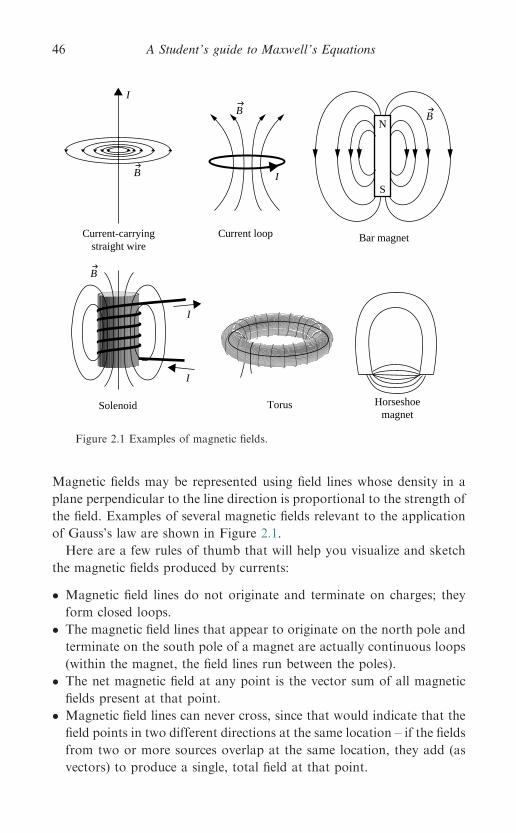
Magnetic fields may be represented using field lines whose density in a

plane perpendicular to the line direction is proportional to the strength of

the field. Examples of several magnetic fields relevant to the application

of Gauss’s law are shown in Figure 2.1.


the magnetic fields produced by currents:

� Magnetic field lines do not originate and terminate on charges; they

form closed loops.

� The magnetic field lines that appear to originate on the north pole and

terminate on the south pole of a magnet are actually continuous loops

(within the magnet, the field lines run between the poles).

� The net magnetic field at any point is the vector sum of all magnetic

fields present at that point.

� Magnetic field lines can never cross, since that would indicate that the

field points in two different directions at the same location – if the fields

from two or more sources overlap at the same location, they add (as

vectors) to produce a single, total field at that point.

I

I

B

N

S

I

I

Current-carryingstraight wire

Current loop Bar magnet

Solenoid Torus Horseshoemagnet

B

B

B

Figure 2.1 Examples of magnetic fields.


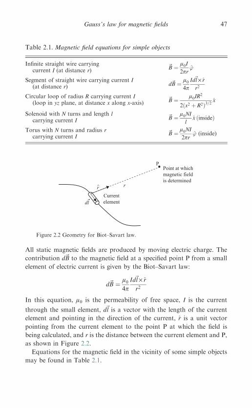
All static magnetic fields are produced by moving electric charge. The

contribution d~B to the magnetic field at a specified point P from a small

element of electric current is given by the Biot–Savart law:

d~B ¼ l04p

Id~l · rr2

In this equation, l0 is the permeability of free space, I is the current

through the small element, d~l is a vector with the length of the current

element and pointing in the direction of the current, r is a unit vector

pointing from the current element to the point P at which the field is

being calculated, and r is the distance between the current element and P,

as shown in Figure 2.2.

Equations for the magnetic field in the vicinity of some simple objects

may be found in Table 2.1.

Table 2.1. Magnetic field equations for simple objects

Infinite straight wire carryingcurrent I (at distance r)

~B ¼ l0I2pr

’

Segment of straight wire carrying current I(at distance r) d~B ¼ l0

4pId~l · rr2

Circular loop of radius R carrying current I(loop in yz plane, at distance x along x-axis)

~B ¼ l0IR2

2ðx2 þ R2Þ3=2x

Solenoid with N turns and length lcarrying current I

~B ¼ l0NIl

x ðinsideÞTorus with N turns and radius r

carrying current I~B ¼ l0NI

2pr’ (inside)

r

P

dl

r

Current element

Point at whichmagnetic field is determined

^

Figure 2.2 Geometry for Biot–Savart law.


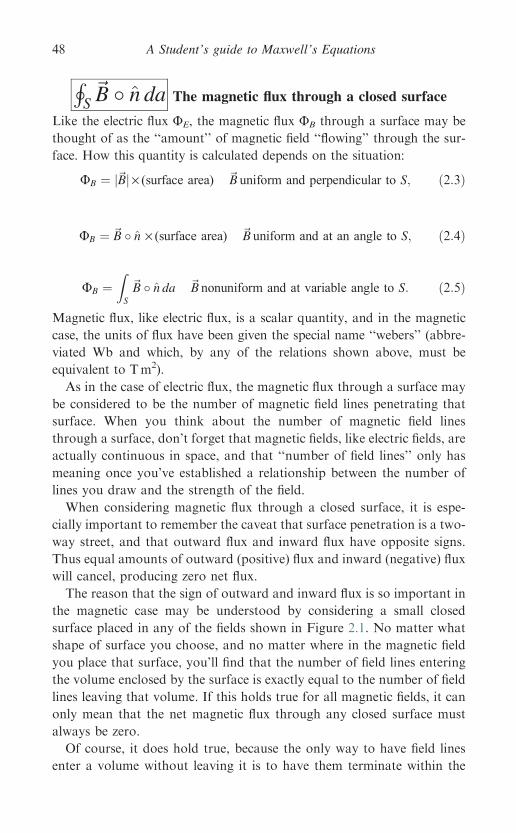
HS~B � n da The magnetic flux through a closed surface

Like the electric flux UE, the magnetic flux UB through a surface may be

thought of as the ‘‘amount’’ of magnetic field ‘‘flowing’’ through the sur-

face. How this quantity is calculated depends on the situation:

UB ¼ j~Bj · (surface area) ~B uniform and perpendicular to S; ð2:3Þ

UB ¼ ~B � n · (surface area) ~B uniform and at an angle to S; ð2:4Þ

UB ¼ZS

~B � n da ~B nonuniform and at variable angle to S: ð2:5Þ

Magnetic flux, like electric flux, is a scalar quantity, and in the magnetic

case, the units of flux have been given the special name ‘‘webers’’ (abbre-

viated Wb and which, by any of the relations shown above, must be

equivalent to Tm2).

As in the case of electric flux, the magnetic flux through a surface may

be considered to be the number of magnetic field lines penetrating that

surface. When you think about the number of magnetic field lines

through a surface, don’t forget that magnetic fields, like electric fields, are

actually continuous in space, and that ‘‘number of field lines’’ only has

meaning once you’ve established a relationship between the number of

lines you draw and the strength of the field.

When considering magnetic flux through a closed surface, it is espe-

cially important to remember the caveat that surface penetration is a two-

way street, and that outward flux and inward flux have opposite signs.

Thus equal amounts of outward (positive) flux and inward (negative) flux

will cancel, producing zero net flux.

The reason that the sign of outward and inward flux is so important in

the magnetic case may be understood by considering a small closed

surface placed in any of the fields shown in Figure 2.1. No matter what

shape of surface you choose, and no matter where in the magnetic field

you place that surface, you’ll find that the number of field lines entering

the volume enclosed by the surface is exactly equal to the number of field

lines leaving that volume. If this holds true for all magnetic fields, it can

only mean that the net magnetic flux through any closed surface must

always be zero.

Of course, it does hold true, because the only way to have field lines

enter a volume without leaving it is to have them terminate within the


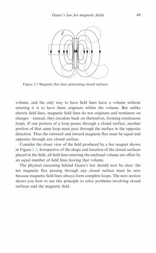
volume, and the only way to have field lines leave a volume without

entering it is to have them originate within the volume. But unlike

electric field lines, magnetic field lines do not originate and terminate on

charges – instead, they circulate back on themselves, forming continuous

loops. If one portion of a loop passes through a closed surface, another

portion of that same loop must pass through the surface in the opposite

direction. Thus the outward and inward magnetic flux must be equal and

opposite through any closed surface.

Consider the closer view of the field produced by a bar magnet shown

in Figure 2.3. Irrespective of the shape and location of the closed surfaces

placed in the field, all field lines entering the enclosed volume are offset by

an equal number of field lines leaving that volume.

The physical reasoning behind Gauss’s law should now be clear: the

net magnetic flux passing through any closed surface must be zero

because magnetic field lines always form complete loops. The next section

shows you how to use this principle to solve problems involving closed

surfaces and the magnetic field.

B

Figure 2.3 Magnetic flux lines penetrating closed surfaces.


HS~B � n da ¼ 0 Applying Gauss’s law (integral form)

In situations involving complex surfaces and fields, finding the flux by

integrating the normal component of the magnetic field over a specified

surface can be quite difficult. In such cases, knowing that the total

magnetic flux through a closed surface must be zero may allow you to

simplify the problem, as demonstrated by the following examples.

Example 2.1: Given an expression for the magnetic field and a surface

geometry, find the flux through a specified portion of that surface.

Problem: A closed cylinder of height h and radius R is placed in a mag-

netic field given by ~B ¼ B0ð j� kÞ. If the axis of the cylinder is aligned

along the z-axis, find the flux through (a) the top and bottom surfaces of

the cylinder and (b) the curved surface of the cylinder.

Solution: Gauss’s law tells you that the magnetic flux through the entire

surface must be zero, so if you’re able to figure out the flux through some

portions of the surface, you can deduce the flux through the other por-

tions. In this case, the flux through the top and bottom of the cylinder are

relatively easy to find; whatever additional amount it takes to make the

total flux equal to zero must come from the curved sides of the cylinder.

Thus

UB;Top þUB;Bottom þUB;Sides ¼ 0:

The magnetic flux through any surface is

UB ¼ZS

~B � n da:

For the top surface, n ¼ k, so

~B � n ¼ ðB0j� B0kÞ � k ¼ �B0:

Thus

UB;Top ¼ZS

~B � n da ¼ �B0

ZS

da ¼ �B0ðpR2Þ:

A similar analysis for the bottom surface (for which n ¼ �k) gives

UB;Bottom ¼ZS

~B � n da ¼ þB0

ZS

da ¼ þB0ðpR2Þ:

Since UB,Top¼�UB,Bottom, you can conclude that UB,Sides¼ 0.


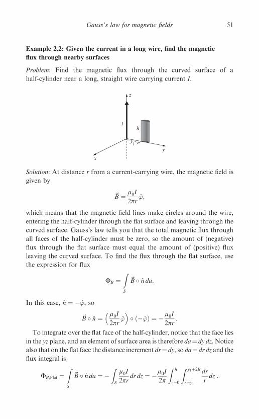
Example 2.2: Given the current in a long wire, find the magnetic

flux through nearby surfaces

Problem: Find the magnetic flux through the curved surface of a

half-cylinder near a long, straight wire carrying current I.

Solution: At distance r from a current-carrying wire, the magnetic field is

given by

~B ¼ l0I2pr

’;

which means that the magnetic field lines make circles around the wire,

entering the half-cylinder through the flat surface and leaving through the

curved surface. Gauss’s law tells you that the total magnetic flux through

all faces of the half-cylinder must be zero, so the amount of (negative)

flux through the flat surface must equal the amount of (positive) flux

leaving the curved surface. To find the flux through the flat surface, use

the expression for flux

UB ¼ZS

~B � n da:

In this case, n ¼ �’, so

~B � n ¼� l0I2pr

’�� ð�’Þ ¼ � l0I

2pr:

To integrate over the flat face of the half-cylinder, notice that the face lies

in the yz plane, and an element of surface area is therefore da¼ dy dz. Notice

also that on the flat face the distance increment dr¼ dy, so da¼ dr dz and the

flux integral is

UB;Flat ¼ZS

~B � n da ¼ �ZS

l0I2pr

dr dz ¼ � l0I2p

Z h

z¼0

Z y1þ2R

r¼y1

dr

rdz :

y1

x

y

z

hI


Thus

UB;Flat ¼ � l0I2p

lny1 þ 2R

y1

� �ðhÞ ¼ � l0Ih

2pln 1þ 2R

y1

� �:

Since the total magnetic flux through this closed surface must be zero, this

means that the flux through the curved side of the half-cylinder is

UB;Curved side ¼ l0Ih2p

ln 1þ 2R

y1

� �:


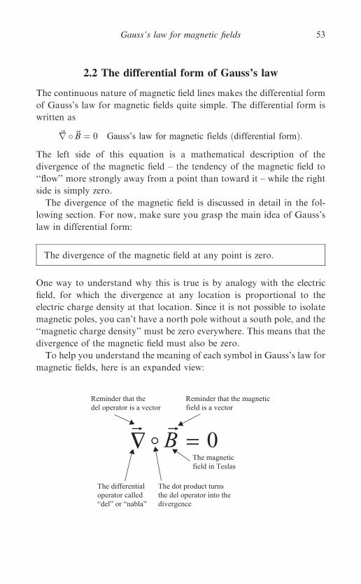
2.2 The differential form of Gauss’s law

The continuous nature of magnetic field lines makes the differential form

of Gauss’s law for magnetic fields quite simple. The differential form is

written as

~r �~B ¼ 0 Gauss’s law for magnetic fields ðdifferential formÞ:The left side of this equation is a mathematical description of the

divergence of the magnetic field – the tendency of the magnetic field to

‘‘flow’’ more strongly away from a point than toward it – while the right

side is simply zero.

The divergence of the magnetic field is discussed in detail in the fol-

lowing section. For now, make sure you grasp the main idea of Gauss’s

law in differential form:

The divergence of the magnetic field at any point is zero.

One way to understand why this is true is by analogy with the electric

field, for which the divergence at any location is proportional to the

electric charge density at that location. Since it is not possible to isolate

magnetic poles, you can’t have a north pole without a south pole, and the

‘‘magnetic charge density’’ must be zero everywhere. This means that the

divergence of the magnetic field must also be zero.

To help you understand the meaning of each symbol in Gauss’s law for

magnetic fields, here is an expanded view:

B 0� =

Reminder that thedel operator is a vector

Reminder that the magneticfield is a vector


The dot product turnsthe del operator into the divergence

The magneticfield in Teslas


~r �~B The divergence of the magnetic field

This expression is the entire left side of the differential form of Gauss’s

law, and it represents the divergence of the magnetic field. Since diver-

gence is by definition the tendency of a field to ‘‘flow’’ away from a point

more strongly than toward that point, and since no point sources or sinks

of the magnetic field have ever been found, the amount of ‘‘incoming’’

field is exactly the same as the amount of ‘‘outgoing’’ field at every point.

So it should not surprise you to find that the divergence of ~B is always

zero.

To verify this for the case of the magnetic field around a long, current-

carrying wire, take the divergence of the expression for the wire’s mag-

netic field as given in Table 2.1:

divð~BÞ ¼~r �~B ¼~r � l0I2pr

’

� �: ð2:6Þ

This is most easily determined using cylindrical coordinates:

~r �~B ¼ 1

r

@

@rrBrð Þ þ 1

r

@Bf

@fþ @Bz

@z: ð2:7Þ

which, since ~B has only a u-component, is

~r �~B ¼ 1

r

@ l0I=2prð Þ@’

¼ 0: ð2:8Þ

You can understand this result using the following reasoning: since

the magnetic field makes circular loops around the wire, it has no radial

or z-dependence. And since the u-component has no u-dependence (that

is, the magnetic field has constant amplitude around any circular path

centered on the wire), the flux away from any point must be the same as

the flux toward that point. This means that the divergence of the mag-

netic field is zero everywhere.

Vector fields with zero divergence are called ‘‘solenoidal’’ fields, and all

magnetic fields are solenoidal.


~r �~B ¼ 0 Applying Gauss’s law (differential form)

Knowing that the divergence of the magnetic field must be zero allows

you to attack problems involving the spatial change in the components of

a magnetic field and to determine whether a specified vector field could be

a magnetic field. This section has examples of such problems.

Example 2.3: Given incomplete information about the components of

a magnetic field, use Gauss’s law to establish relationships between those

components

Problem: A magnetic field is given by the expression

~B ¼ axz iþ byz jþ ck

What is the relationship between a and b?

Solution: You know from Gauss’s law for magnetic fields that the

divergence of the magnetic field must be zero. Thus

~r �~B ¼ @Bx

@xþ @By

@yþ @Bz

@z¼ 0:

Thus

@ðaxzÞ@x

þ @ðbyzÞ@y

þ @c

@z¼ 0

and

azþ bzþ 0 ¼ 0;

which means that a¼�b.

Example 2.4: Given an expression for a vector field, determine whether

that field could be a magnetic field.

Problem: A vector field is given by the expression

~Aðx; yÞ ¼ a cosðbxÞiþ aby sinðbxÞj:Could this field be a magnetic field?

Solution: Gauss’s law tells you that the divergence of all magnetic fields

must be zero, and checking the divergence of this vector field gives


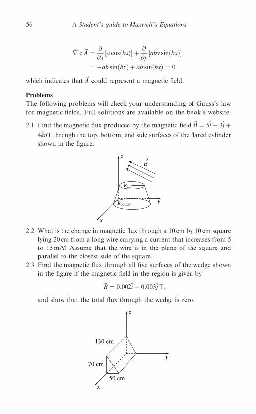
~r �~A ¼ @

@x½a cosðbxÞ� þ @

@y½aby sinðbxÞ�

¼ �ab sinðbxÞ þ ab sinðbxÞ ¼ 0

which indicates that ~A could represent a magnetic field.

Problems

The following problems will check your understanding of Gauss’s law

for magnetic fields. Full solutions are available on the book’s website.

2.1 Find the magnetic flux produced by the magnetic field ~B ¼ 5i� 3jþ4knT through the top, bottom, and side surfaces of the flared cylinder

shown in the figure.

2.2 What is the change in magnetic flux through a 10 cm by 10 cm square

lying 20 cm from a long wire carrying a current that increases from 5

to 15mA? Assume that the wire is in the plane of the square and

parallel to the closest side of the square.

2.3 Find the magnetic flux through all five surfaces of the wedge shown

in the figure if the magnetic field in the region is given by

~B ¼ 0:002iþ 0:003jT;

and show that the total flux through the wedge is zero.

Rtop

Rbottom

x

y

zB

x

y

z

50 cm

70 cm

130 cm


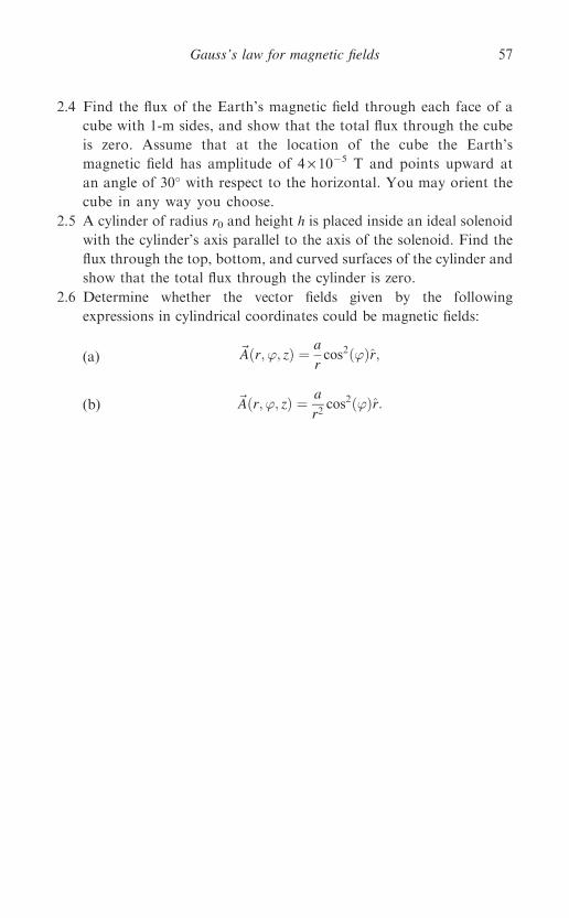
2.4 Find the flux of the Earth’s magnetic field through each face of a

cube with 1-m sides, and show that the total flux through the cube

is zero. Assume that at the location of the cube the Earth’s

magnetic field has amplitude of 4 · 10�5 T and points upward at

an angle of 30� with respect to the horizontal. You may orient the

cube in any way you choose.

2.5 A cylinder of radius r0 and height h is placed inside an ideal solenoid

with the cylinder’s axis parallel to the axis of the solenoid. Find the

flux through the top, bottom, and curved surfaces of the cylinder and

show that the total flux through the cylinder is zero.

2.6 Determine whether the vector fields given by the following

expressions in cylindrical coordinates could be magnetic fields:

(a) ~Aðr; ’; zÞ ¼ a

rcos2ð’Þr;

(b) ~Aðr; ’; zÞ ¼ a

r2cos2ð’Þr:


3

Faraday’s law

In a series of epoch-making experiments in 1831, Michael Faraday

demonstrated that an electric current may be induced in a circuit by

changing the magnetic flux enclosed by the circuit. That discovery is

made even more useful when extended to the general statement that a

changing magnetic field produces an electric field. Such ‘‘induced’’ elec-

tric fields are very different from the fields produced by electric charge,

and Faraday’s law of induction is the key to understanding their

behavior.

3.1 The integral form of Faraday’s law

In many texts, the integral form of Faraday’s law is written as

IC

~E � d~l ¼ � d

dt

ZS

~B � n da Faraday’s law ðintegral formÞ:

Some authors feel that this form is misleading because it confounds two

distinct phenomena: magnetic induction (involving a changing magnetic

field) and motional electromotive force (emf) (involving movement of a

charged particle through a magnetic field). In both cases, an emf is

produced, but only magnetic induction leads to a circulating electric field

in the rest frame of the laboratory. This means that this common version

of Faraday’s law is rigorously correct only with the caveat that ~E rep-

resents the electric field in the rest frame of each segment d~l of the path of

integration.

58

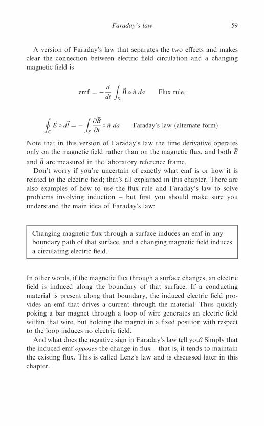
A version of Faraday’s law that separates the two effects and makes

clear the connection between electric field circulation and a changing

magnetic field is

emf ¼ � d

dt

ZS

~B � n da Flux rule,

IC

~E � d~l ¼ �ZS

@~B

@t� n da Faraday’s law ðalternate formÞ:

Note that in this version of Faraday’s law the time derivative operates

only on the magnetic field rather than on the magnetic flux, and both ~E

and ~B are measured in the laboratory reference frame.

Don’t worry if you’re uncertain of exactly what emf is or how it is

related to the electric field; that’s all explained in this chapter. There are

also examples of how to use the flux rule and Faraday’s law to solve

problems involving induction – but first you should make sure you

understand the main idea of Faraday’s law:

Changing magnetic flux through a surface induces an emf in any

boundary path of that surface, and a changing magnetic field induces

a circulating electric field.

In other words, if the magnetic flux through a surface changes, an electric

field is induced along the boundary of that surface. If a conducting

material is present along that boundary, the induced electric field pro-

vides an emf that drives a current through the material. Thus quickly

poking a bar magnet through a loop of wire generates an electric field

within that wire, but holding the magnet in a fixed position with respect

to the loop induces no electric field.

And what does the negative sign in Faraday’s law tell you? Simply that

the induced emf opposes the change in flux – that is, it tends to maintain

the existing flux. This is called Lenz’s law and is discussed later in this

chapter.

Faraday’s law 59

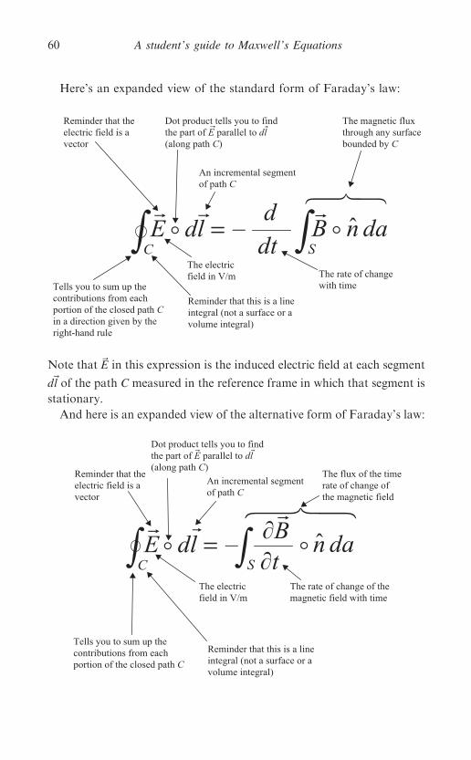
Here’s an expanded view of the standard form of Faraday’s law:

Note that ~E in this expression is the induced electric field at each segment

d~l of the path C measured in the reference frame in which that segment is

stationary.

And here is an expanded view of the alternative form of Faraday’s law:

=C

d–dl

dtE

The electricfield in V/m


Reminder that this is a lineintegral (not a surface or avolume integral)

An incremental segmentof path C

Tells you to sum up thecontributions from eachportion of the closed path Cin a direction given by theright-hand rule

ˆS

danB

Dot product tells you to findthe part of E parallel to dl(along path C)

The rate of changewith time

The magnetic fluxthrough any surfacebounded by C

∫ ∫

=C

–dlE



Dot product tells you to findthe part of E parallel to dl(along path C)

Reminder that this is a lineintegral (not a surface or avolume integral)

Tells you to sum up thecontributions from eachportion of the closed path C

ˆS

dan

The rate of change of themagnetic field with time

An incremental segmentof path C

The flux of the timerate of change of the magnetic field

∫ ∫


In this case, ~E represents the electric field in the laboratory frame of

reference (the same frame in which ~B is measured).

Faraday’s law and the flux rule can be used to solve a variety of

problems involving changing magnetic flux and induced electric fields, in

particular problems of two types:

(1) Given information about the changing magnetic flux, find the

induced emf.

(2) Given the induced emf on a specified path, determine the rate of

change of the magnetic field magnitude or direction or the area

bounded by the path.

In situations of high symmetry, in addition to finding the induced emf, it

is also possible to find the induced electric field when the rate of change of

the magnetic field is known.

Faraday’s law 61

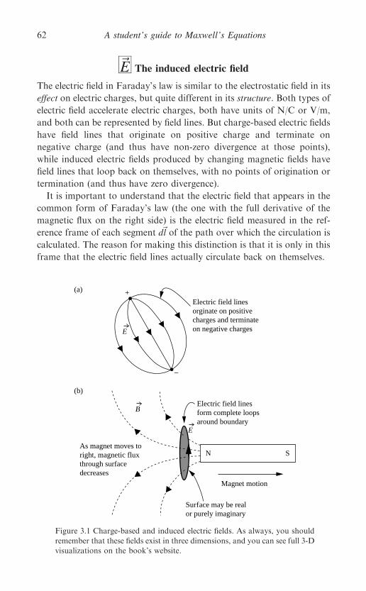
~E The induced electric field

The electric field in Faraday’s law is similar to the electrostatic field in its

effect on electric charges, but quite different in its structure. Both types of

electric field accelerate electric charges, both have units of N/C or V/m,

and both can be represented by field lines. But charge-based electric fields

have field lines that originate on positive charge and terminate on

negative charge (and thus have non-zero divergence at those points),

while induced electric fields produced by changing magnetic fields have

field lines that loop back on themselves, with no points of origination or

termination (and thus have zero divergence).

It is important to understand that the electric field that appears in the

common form of Faraday’s law (the one with the full derivative of the

magnetic flux on the right side) is the electric field measured in the ref-

erence frame of each segment d~l of the path over which the circulation is

calculated. The reason for making this distinction is that it is only in this

frame that the electric field lines actually circulate back on themselves.

E

+

–

Electric field linesorginate on positivecharges and terminateon negative charges

(a)

N

Magnet motion

B

E

Electric field linesform complete loopsaround boundary

As magnet moves toright, magnetic fluxthrough surfacedecreases

Surface may be realor purely imaginary

S

(b)

Figure 3.1 Charge-based and induced electric fields. As always, you should

remember that these fields exist in three dimensions, and you can see full 3-D

visualizations on the book’s website.


Examples of a charge-based and an induced electric field are shown in

Figure 3.1.

Note that the induced electric field in Figure 3.1(b) is directed so as to

drive an electric current that produces magnetic flux that opposes the

change in flux due to the changing magnetic field. In this case, the motion of

the magnet to the right means that the leftward magnetic flux is decreasing,

so the induced current produces additional leftward magnetic flux.


the electric fields produced by changing magnetic fields:

� Induced electric field lines produced by changing magnetic fields must

form complete loops.

� The net electric field at any point is the vector sum of all electric fields

present at that point.

� Electric field lines can never cross, since that would indicate that the

field points in two different directions at the same location.

In summary, the~E in Faraday’s law represents the induced electric field at

each point along path C, a boundary of the surface through which the

magnetic flux is changing over time. The path may be through empty

space or through a physical material – the induced electric field exists in

either case.

Faraday’s law 63

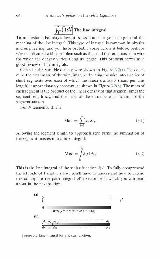
HCðÞdl The line integral

To understand Faraday’s law, it is essential that you comprehend the

meaning of the line integral. This type of integral is common in physics

and engineering, and you have probably come across it before, perhaps

when confronted with a problem such as this: find the total mass of a wire

for which the density varies along its length. This problem serves as a

good review of line integrals.

Consider the variable-density wire shown in Figure 3.2(a). To deter-

mine the total mass of the wire, imagine dividing the wire into a series of

short segments over each of which the linear density k (mass per unit

length) is approximately constant, as shown in Figure 3.2(b). The mass of

each segment is the product of the linear density of that segment times the

segment length dxi, and the mass of the entire wire is the sum of the

segment masses.

For N segments, this is

Mass ¼XNi¼1

ki dxi: ð3:1Þ

Allowing the segment length to approach zero turns the summation of

the segment masses into a line integral:

Mass ¼ZL0

kðxÞ dx: ð3:2Þ

This is the line integral of the scalar function k(x). To fully comprehend

the left side of Faraday’s law, you’ll have to understand how to extend

this concept to the path integral of a vector field, which you can read

about in the next section.

x0 L

Density varies with x: λ = λ (x)

1 2 3

dx1 dx2 dx3 dxN

(a)

(b)λ λ λ Nλ

Figure 3.2 Line integral for a scalar function.


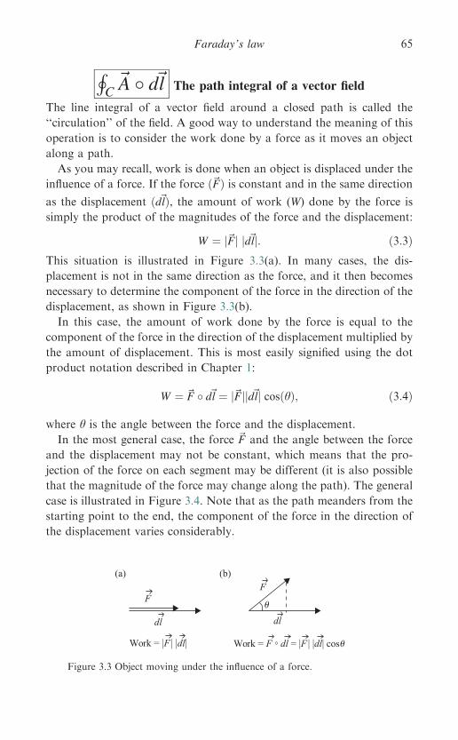
HC~A � d~l The path integral of a vector field

The line integral of a vector field around a closed path is called the

‘‘circulation’’ of the field. A good way to understand the meaning of this

operation is to consider the work done by a force as it moves an object

along a path.

As you may recall, work is done when an object is displaced under the

influence of a force. If the force ð~FÞ is constant and in the same direction

as the displacement ðd~lÞ, the amount of work (W) done by the force is

simply the product of the magnitudes of the force and the displacement:

W ¼ j~Fj jd~lj: ð3:3ÞThis situation is illustrated in Figure 3.3(a). In many cases, the dis-

placement is not in the same direction as the force, and it then becomes

necessary to determine the component of the force in the direction of the

displacement, as shown in Figure 3.3(b).

In this case, the amount of work done by the force is equal to the

component of the force in the direction of the displacement multiplied by

the amount of displacement. This is most easily signified using the dot

product notation described in Chapter 1:

W ¼ ~F � d~l ¼ j~Fjjd~lj cosðhÞ; ð3:4Þ

where h is the angle between the force and the displacement.

In the most general case, the force ~F and the angle between the force

and the displacement may not be constant, which means that the pro-

jection of the force on each segment may be different (it is also possible

that the magnitude of the force may change along the path). The general

case is illustrated in Figure 3.4. Note that as the path meanders from the

starting point to the end, the component of the force in the direction of

the displacement varies considerably.

FF

dl dl

u

Work = F ° dl = |F | |dl| cos uWork = |F | |dl|

(a) (b)

Figure 3.3 Object moving under the influence of a force.

Faraday’s law 65

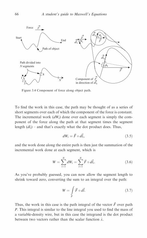
To find the work in this case, the path may be thought of as a series of

short segments over each of which the component of the force is constant.

The incremental work (dWi) done over each segment is simply the com-

ponent of the force along the path at that segment times the segment

length (dli) – and that’s exactly what the dot product does. Thus,

dWi ¼ ~F � d~li; ð3:5Þ

and the work done along the entire path is then just the summation of the

incremental work done at each segment, which is

W ¼XNi¼1

dWi ¼XNi¼1

~F � d~li: ð3:6Þ

As you’ve probably guessed, you can now allow the segment length to

shrink toward zero, converting the sum to an integral over the path:

W ¼ZP

~F � d~l: ð3:7Þ

Thus, the work in this case is the path integral of the vector ~F over path

P. This integral is similar to the line integral you used to find the mass of

a variable-density wire, but in this case the integrand is the dot product

between two vectors rather than the scalar function k.

StartEnd

Path of object

F

Path divided into N segments

dl1

dl8

12

3

8

N

FF

u8

u1

Component of F in direction of dl8

dl8

F

u8

Force

Figure 3.4 Component of force along object path.


Although the force in this example is uniform, the same analysis

pertains to a vector field of force that varies in magnitude and direction

along the path. The integral on the right side of Equation 3.7 may be

defined for any vector field ~A and any path C. If the path is closed, this

integral represents the circulation of the vector field around that path:

Circulation �IC

~A � d~l: ð3:8Þ

The circulation of the electric field is an important part of Faraday’s law,

as described in the next section.

Faraday’s law 67

HC~E � d~l The electric field circulation

Since the field lines of induced electric fields form closed loops, these

fields are capable of driving charged particles around continuous circuits.

Charge moving through a circuit is the very definition of electric current,

so the induced electric field may act as a generator of electric current. It is

therefore understandable that the circulation of the electric field around a

circuit has come to be known as an ‘‘electromotive force’’:

electromotive force ðemfÞ ¼IC

~E � d~l: ð3:9Þ

Of course, the path integral of an electric field is not a force (which must

have SI units of newtons), but rather a force per unit charge integrated

over a distance (with units of newtons per coulomb times meters, which

are the same as volts). Nonetheless, the terminology is now standard, and

‘‘source of emf’’ is often applied to induced electric fields as well as to

batteries and other sources of electrical energy.

So, exactly what is the circulation of the induced electric field around a

path? It is just the work done by the electric field in moving a unit charge

around that path, as you can see by substituting ~F=q for ~E in the circu-

lation integral: IC

~E � d~l ¼IC

~F

q� d~l ¼

HC~F � d~lq

¼ W

q: ð3:10Þ

Thus, the circulation of the induced electric field is the energy given to

each coulomb of charge as it moves around the circuit.


ddt

RS~B � n da The rate of change of flux

The right side of the common form of Faraday’s law may look intimi-

dating at first glance, but a careful inspection of the terms reveals that the

largest portion of this expression is simply the magnetic flux ðUBÞ:

UB ¼ZS

~B � n da:

If you’re tempted to think that this quantity must be zero according to

Gauss’s law for magnetic fields, look more carefully. The integral in this

expression is over any surface S, whereas the integral in Gauss’s law is

specifically over a closed surface. The magnetic flux (proportional to the

number of magnetic field lines) through an open surface may indeed be

nonzero – it is only when the surface is closed that the number of mag-

netic field lines passing through the surface in one direction must equal

the number passing through in the other direction.

So the right side of this form of Faraday’s law involves the magnetic

flux through any surface S – more specifically, the rate of change with

time (d/dt) of that flux. If you’re wondering how the magnetic flux

through a surface might change, just look at the equation and ask

yourself what might vary with time in this expression. Here are three

possibilities, each of which is illustrated in Figure 3.5:

� The magnitude of ~B might change: the strength of the magnetic field

may be increasing or decreasing, causing the number of field lines

penetrating the surface to change.

� The angle between~B and the surface normal might change: varying the

direction of either ~B or the surface normal causes ~B � n to change.

� The area of the surface might change: even if the magnitude of ~B and

the direction of both ~B and n remain the same, varying the area of

surface S will change the value of the flux through the surface.

Each of these changes, or a combination of them, causes the right side of

Faraday’s law to become nonzero. And since the left side of Faraday’s

law is the induced emf, you should now understand the relationship

between induced emf and changing magnetic flux.

To connect the mathematical statement of Faraday’s law to physical

effects, consider the magnetic fields and conducting loops shown in

Figure 3.5. As Faraday discovered, the mere presence of magnetic flux

Faraday’s law 69

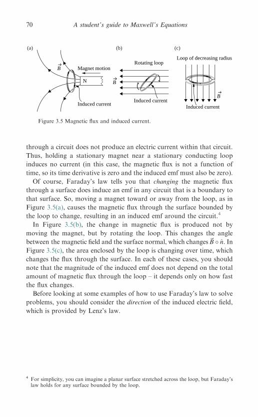
through a circuit does not produce an electric current within that circuit.

Thus, holding a stationary magnet near a stationary conducting loop

induces no current (in this case, the magnetic flux is not a function of

time, so its time derivative is zero and the induced emf must also be zero).

Of course, Faraday’s law tells you that changing the magnetic flux

through a surface does induce an emf in any circuit that is a boundary to

that surface. So, moving a magnet toward or away from the loop, as in

Figure 3.5(a), causes the magnetic flux through the surface bounded by

the loop to change, resulting in an induced emf around the circuit.4

In Figure 3.5(b), the change in magnetic flux is produced not by

moving the magnet, but by rotating the loop. This changes the angle

between the magnetic field and the surface normal, which changes~B � n. InFigure 3.5(c), the area enclosed by the loop is changing ove r tim e, whi ch

changes the flux through the surface. In each of these cases, you should

note that the magnitude of the induced emf does not depend on the total

amount of magnetic flux through the loop – it depends only on how fast

the flux changes.

Before looking at some examples of how to use Faraday’s law to solve

problems, you should consider the direction of the induced electric field,

which is provided by Lenz’s law.

B

Rotating loop

B

Loop of decreasing radius

N

Magnet motionB

Induced currentInduced current

Induced current

(a) (b) (c)

Figure 3.5 Magnetic flux and induced current.

4 For simplicity, you can imagine a planar surface stretched across the loop, but Faraday’slaw holds for any surface bounded by the loop.


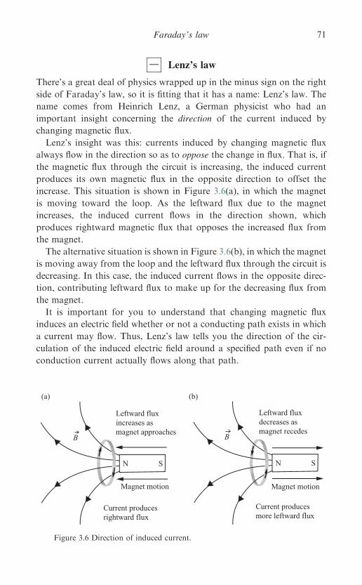
� Lenz’s law

There’s a great deal of physics wrapped up in the minus sign on the right

side of Faraday’s law, so it is fitting that it has a name: Lenz’s law. The

name comes from Heinrich Lenz, a German physicist who had an

important insight concerning the direction of the current induced by

changing magnetic flux.

Lenz’s insight was this: currents induced by changing magnetic flux

always flow in the direction so as to oppose the change in flux. That is, if

the magnetic flux through the circuit is increasing, the induced current

produces its own magnetic flux in the opposite direction to offset the

increase. This situation is shown in Figure 3.6(a), in which the magnet

is moving toward the loop. As the leftward flux due to the magnet

increases, the induced current flows in the direction shown, which

produces rightward magnetic flux that opposes the increased flux from

the magnet.

The alternative situation is shown in Figure 3.6(b), in which the magnet

is moving away from the loop and the leftward flux through the circuit is

decreasing. In this case, the induced current flows in the opposite direc-

tion, contributing leftward flux to make up for the decreasing flux from

the magnet.

It is important for you to understand that changing magnetic flux

induces an electric field whether or not a conducting path exists in which

a current may flow. Thus, Lenz’s law tells you the direction of the cir-

culation of the induced electric field around a specified path even if no

conduction current actually flows along that path.

N S

Magnet motion

B

(a) (b)

Leftward flux increases as magnet approaches

Current produces rightward flux

N S

Magnet motion

Leftward flux decreases as magnet recedes

Current produces more leftward flux

B

Figure 3.6 Direction of induced current.

Faraday’s law 71

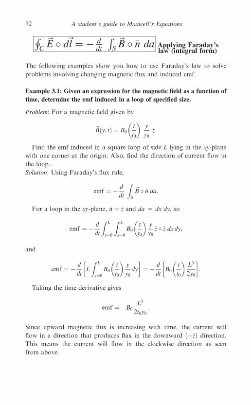
HC~E � d~l ¼ � d

dt

RS~B � n da Applying Faraday’s

law (integral form)

The following examples show you how to use Faraday’s law to solve

problems involving changing magnetic flux and induced emf.

Example 3.1: Given an expression for the magnetic field as a function of

time, determine the emf induced in a loop of specified size.

Problem: For a magnetic field given by

~Bðy; tÞ ¼ B0t

t0

� �y

y0z:

Find the emf induced in a square loop of side L lying in the xy-plane

with one corner at the origin. Also, find the direction of current flow in

the loop.

Solution: Using Faraday’s flux rule,

emf ¼ � d

dt

ZS

~B � n da:

For a loop in the xy-plane, n ¼ z and da = dx dy, so

emf ¼ � d

dt

Z L

y¼0

Z L

x¼0

B0t

t0

� �y

y0z � z dx dy,

and

emf ¼ � d

dtL

Z L

y¼0

B0t

t0

� �y

y0dy

� ¼ � d

dtB0

t

t0

� �L3

2y0

� :

Taking the time derivative gives

emf ¼ �B0L3

2t0y0:

Since upward magnetic flux is increasing with time, the current will

flow in a direction that produces flux in the downward ð�zÞ direction.

This means the current will flow in the clockwise direction as seen

from above.


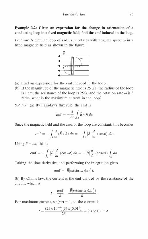
Example 3.2: Given an expression for the change in orientation of a

conducting loop in a fixed magnetic field, find the emf induced in the loop.

Problem: A circular loop of radius r0 rotates with angular speed x in a

fixed magnetic field as shown in the figure.

(a) Find an expression for the emf induced in the loop.

(b) If the magnitude of the magnetic field is 25 lT, the radius of the loopis 1 cm, the resistance of the loop is 25W, and the rotation rate x is 3

rad/s, what is the maximum current in the loop?

Solution: (a) By Faraday’s flux rule, the emf is

emf ¼ � d

dt

ZS

~B � n da

Since the magnetic field and the area of the loop are constant, this becomes

emf ¼ �ZS

d

dtð~B � nÞ da ¼ �

ZS

~B d

dtðcos hÞ da:

Using h=xt, this is

emf ¼ �ZS

~B d

dtðcosxtÞ da ¼ � ~B

ddt

ðcosxtÞZS

da:

Taking the time derivative and performing the integration gives

emf ¼ ~B xðsinxtÞðpr20Þ:

(b) By Ohm’s law, the current is the emf divided by the resistance of the

circuit, which is

I ¼ emf

R¼

~B xðsinxtÞðpr20Þ

R:

For maximum current, sin(xt)=1, so the current is

I ¼ ð25· 10�6Þð3Þ½pð0:012Þ�25

¼ 9:4 · 10�10A:

Bv

Faraday’s law 73

Example 3.3: Given an expression for the change in size of a conducting

loop in a fixed magnetic field, find the emf induced in the loop.

Problem: A circular loop lying perpendicular to a fixed magnetic field

decreases in size over time. If the radius of the loop is given by r(t) =

r0(1�t/t0), find the emf induced in the loop.

Solution: Since the loop is perpendicular to the magnetic field, the loop

normal is parallel to ~B, and Faraday’s flux rule is

emf ¼ � d

dt

ZS

~B � n da ¼ � ~B d

dt

ZS

da ¼ � ~B d

dtðpr2Þ:

Inserting r(t) and taking the time derivative gives

emf ¼ � ~B d

dt

�pr20 1� t

t0

� �2¼ � ~B

�pr20ð2Þ 1� t

t0

� �� 1

t0

� �;

or

emf ¼ 2 ~B pr20t0

1� t

t0

� �:


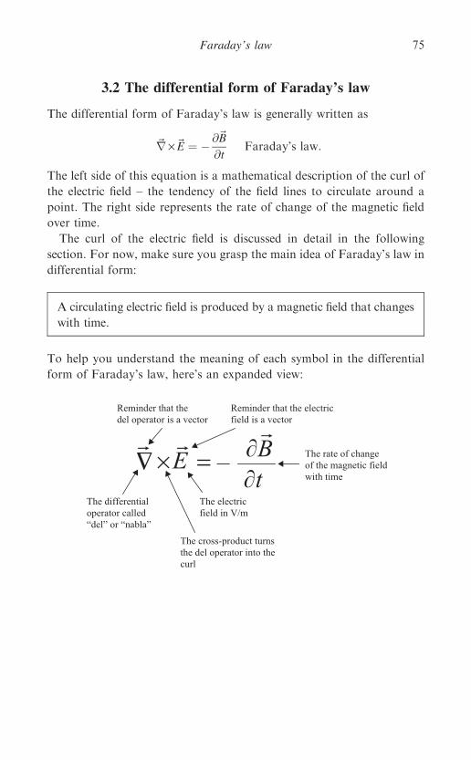
3.2 The differential form of Faraday’s law

The differential form of Faraday’s law is generally written as

~r ·~E ¼ � @~B

@tFaraday’s law:

The left side of this equation is a mathematical description of the curl of

the electric field – the tendency of the field lines to circulate around a

point. The right side represents the rate of change of the magnetic field

over time.

The curl of the electric field is discussed in detail in the following

section. For now, make sure you grasp the main idea of Faraday’s law in

differential form:

A circulating electric field is produced by a magnetic field that changes

with time.


form of Faraday’s law, here’s an expanded view:

E� =

Reminder that thedel operator is a vector

Reminder that the electricfield is a vector


The cross-product turnsthe del operator into the curl


× �B–

�tThe rate of changeof the magnetic fieldwith time

Faraday’s law 75

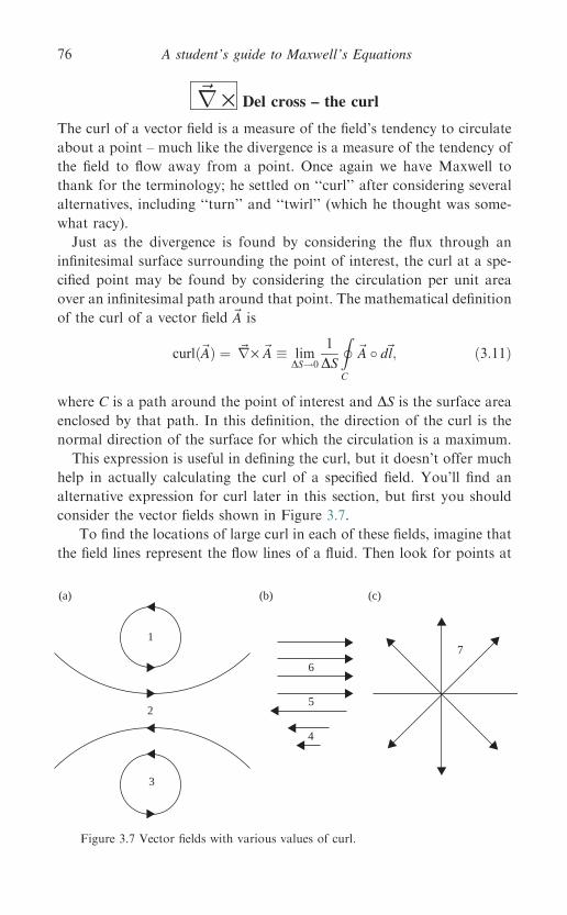
~r · Del cross – the curl

The curl of a vector field is a measure of the field’s tendency to circulate

about a point – much like the divergence is a measure of the tendency of

the field to flow away from a point. Once again we have Maxwell to

thank for the terminology; he settled on ‘‘curl’’ after considering several

alternatives, including ‘‘turn’’ and ‘‘twirl’’ (which he thought was some-

what racy).

Just as the divergence is found by considering the flux through an

infinitesimal surface surrounding the point of interest, the curl at a spe-

cified point may be found by considering the circulation per unit area

over an infinitesimal path around that point. The mathematical definition

of the curl of a vector field ~A is

curlð~AÞ ¼ ~r· ~A � limDS!0

1

DS

IC

~A � d~l; ð3:11Þ

where C is a path around the point of interest and DS is the surface area

enclosed by that path. In this definition, the direction of the curl is the

normal direction of the surface for which the circulation is a maximum.

This expression is useful in defining the curl, but it doesn’t offer much

help in actually calculating the curl of a specified field. You’ll find an

alternative expression for curl later in this section, but first you should

consider the vector fields shown in Figure 3.7.

To find the locations of large curl in each of these fields, imagine that

the field lines represent the flow lines of a fluid. Then look for points at

1

3

5

4

7

2

6

(a) (b) (c)

Figure 3.7 Vector fields with various values of curl.


which the flow vectors on one side of the point are significantly different

(in magnitude, direction, or both) from the flow vectors on the opposite

side of the point.

To aid this thought experiment, imagine holding a tiny paddlewheel at

each point in the flow. If the flow would cause the paddlewheel to rotate,

the center of the wheel marks a point of nonzero curl. The direction of the

curl is along the axis of the paddlewheel (as a vector, curl must have both

magnitude and direction). By convention, the positive-curl direction is

determined by the right-hand rule: if you curl the fingers of your right hand

along the circulation, your thumb points in the direction of positive curl.

Using the paddlewheel test, you can see that points 1, 2, and 3 in

Figure 3.7(a) and points 4 and 5 in Figure 3.7(b) are high-curl locations.

The uniform flow around point 6 in Figure 3.7(b) and the diverging flow

lines around point 7 in Figure 3.7(b) would not cause a tiny paddlewheel

to rotate, meaning that these are points of low or zero curl.

To make this quantitative, you can use the differential form of the curl

or ‘‘del cross’’ ð~r·Þ operator in Cartesian coordinates:

~r· ~A ¼ i@

@xþ j

@

@yþ k

@

@z

� �· ðiAx þ jAy þ kAzÞ: ð3:12Þ

The vector cross-product may be written as a determinant:

~r· ~A ¼i j k@@x

@@y

@@z

Ax Ay Az

; ð3:13Þ

which expands to

~r· ~A ¼ @Az

@y� @Ay

@z

� �iþ @Ax

@z� @Az

@x

� �jþ @Ay

@x� @Ax

@y

� �k: ð3:14Þ

Note that each component of the curl of ~A indicates the tendency of the

field to rotate in one of the coordinate planes. If the curl of the field at a

point has a large x-component, it means that the field has significant

circulation about that point in the y–z plane. The overall direction of the

curl represents the axis about which the rotation is greatest, with the

sense of the rotation given by the right-hand rule.

If you’re wondering how the terms in this equation measure rotation,

consider the vector fields shown in Figure 3.8. Look first at the field in

Faraday’s law 77

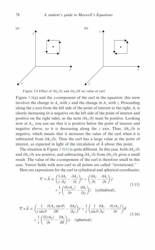
Figure 3.8(a) and the x-component of the curl in the equation: this term

involves the change in Az with y and the change in Ay with z. Proceeding

along the y-axis from the left side of the point of interest to the right, Az is

clearly increasing (it is negative on the left side of the point of interest and

positive on the right side), so the term @Az/@y must be positive. Looking

now at Ay, you can see that it is positive below the point of interest and

negative above, so it is decreasing along the z axis. Thus, @Ay/@z is

negative, which means that it increases the value of the curl when it is

subtracted from @Az/@y. Thus the curl has a large value at the point of

interest, as expected in light of the circulation of ~A about this point.

The situation in Figure 3.8(b) is quite different. In this case, both @Ay/@z

and @Az/@y are positive, and subtracting @Ay/@z from @Az/@y gives a small

result. The value of the x-component of the curl is therefore small in this

case. Vector fields with zero curl at all points are called ‘‘irrotational.’’

Here are expressions for the curl in cylindrical and spherical coordinates:

r · ~A � 1

r

@Az

@’� @A’

@z

� �r þ @Ar

@z� @Az

@r

� �’

þ 1

r

@ðrA’Þ@r

� @Ar

@’

� �z ðcylindricalÞ;

ð3:15Þ

r ·~A � 1

r sin h

@ðA’ sin hÞ@h

� @Ah

@’

� �r þ 1

r

1

sin h@Ar

@’� @ðrA’Þ

@r

� �h

þ 1

r

@ðrAhÞ@r

� @Ar

@h

� �’ ðsphericalÞ:

ð3:16Þ

x

y

z

x

y

z(a) (b)

Figure 3.8 Effect of @Ay/@z and @Az/@Y on value of curl.


~r·~E The curl of the electric field

Since charge-based electric fields diverge away from points of positive

charge and converge toward points of negative charge, such fields cannot

circulate back on themselves. You can understand that by looking at the

field lines for the electric dipole shown in Figure 3.9(a). Imagine moving

along a closed path that follows one of the electric field lines diverging

from the positive charge, such as the dashed line shown in the figure. To

close the loop and return to the positive charge, you’ll have to move

‘‘upstream’’ against the electric field for a portion of the path. For that

segment, ~E � d~l is negative, and the contribution from this part of the

path subtracts from the positive value of~E � d~l for the portion of the path

in which ~E and d~l are in the same direction. Once you’ve gone all the way

around the loop, the integration of ~E � d~l yields exactly zero.

Thus, the field of the electric dipole, like all electrostatic fields, has

no curl.

Electric fields induced by changing magnetic fields are very different, as

you can see in Figure 3.9(b). Wherever a changing magnetic field exists, a

circulating electric field is induced. Unlike charge-based electric fields,

induced fields have no origination or termination points – they are

continuous and circulate back on themselves. Integrating ~E � d~l aroundany boundary path for the surface through which ~B is changing produces

a nonzero result, which means that induced electric fields have curl. The

faster ~B changes, the larger the magnitude of the curl of the induced

electric field.

1 2

∂B/∂t(a) (b)E

E

E E

Figure 3.9 Closed paths in charge-based and induced electric fields.

Faraday’s law 79

~r· ~E ¼ � @~B@t Applying Faraday’s law (differential form)

The differential form of Faraday’s law is very useful in deriving the

electromagnetic wave equation, which you can read about in Chapter 5.

You may also encounter two types of problems that can be solved using

this equation. In one type, you’re provided with an expression for the

magnetic field as a function of time and asked to find the curl of the

induced electric field. In the other type, you’re given an expression for the

induced vector electric field and asked to determine the time rate of

change of the magnetic field. Here are two examples of such problems.

Example 3.4: Given an expression for the magnetic field as a function of

time, find the curl of the electric field.

Problem: The magnetic field in a certain region is given by the expression

~BðtÞ ¼ B0 cosðkz� xtÞ j.(a) Find the curl of the induced electric field at that location.

(b) If the Ez is known to be zero, find Ex.

Solution: (a) By Faraday’s law, the curl of the electric field is the negative

of the derivative of the vector magnetic field with respect to time. Thus,

~r· ~E ¼ � @~B

@t¼ � @ B0 cosðkz� xtÞ½ � j

@t;

or

~r· ~E ¼ �xB0 sinðkz� xtÞ j:(b) Writing out the components of the curl gives

@Ez

@y� @Ey

@z

� �iþ @Ex

@z� @Ez

@x

� �jþ @Ey

@x� @Ex

@y

� �k ¼ �xB0 sinðkz� xtÞj:

Equating the j components and setting Ez to zero gives

@Ex

@z

� �¼ �xB0 sinðkz� xtÞ:

Integrating over z gives

Ex ¼Z�xB0 sinðkz� xtÞdz ¼ x

kB0 cosðkz� xtÞ,

to within a constant of integration.


Example 3.5: Given an expression for the induced electric field, find the

time rate of change of the magnetic field.

Problem: Find the rate of change with time of the magnetic field at a

location at which the induced electric field is given by

~Eðx; y; zÞ ¼ E0z

z0

� �2

iþ x

x0

� �2

jþ y

y0

� �2

k

" #:

Solution: Faraday’s law tells you that the curl of the induced electric field

is equal to the negative of the time rate of change of the magnetic field.

Thus

@~B

@t¼ �~r · ~E;

which in this case gives

@~B

@t¼ � @Ez

@y� @Ey

@z

� �i� @Ex

@z� @Ez

@x

� �j� @Ey

@x� @Ex

@y

� �k,

@~B

@t¼ �E0

2y

y20

� �iþ 2z

z20

� �jþ 2x

x20

� �k

� :

Problems

You can exercise your understanding of Faraday’s law on the following

problems. Full solutions are available on the book’s website.

3.1 Find the emf induced in a square loop with sides of length a lying in

the yz-plane in a region in which the magnetic field changes over time

as ~BðtÞ ¼ B0e�5t=t0 i.

3.2 A square conducting loop with sides of length L rotates so that the

angle between the normal to the plane of the loop and a fixed

magnetic field ~B varies as h(t)¼ h0(t/t0); find the emf induced in the

loop.

3.3 A conducting bar descends with speed v down conducting rails in the

presence of a constant, uniform magnetic field pointing into the page,

as shown in the figure.

(a) Write an expression for the emf induced in the loop.

(b) Determine the direction of current flow in the loop.

Faraday’s law 81

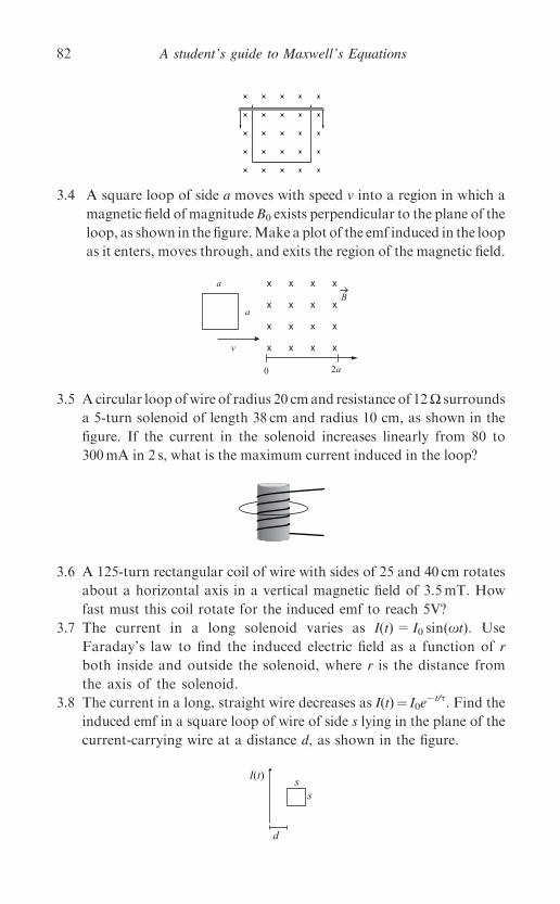
3.4 A square loop of side a moves with speed v into a region in which a

magnetic field of magnitude B0 exists perpendicular to the plane of the

loop, as shown in the figure.Make a plot of the emf induced in the loop

as it enters, moves through, and exits the region of the magnetic field.

3.5 A circular loop ofwire of radius 20 cmand resistance of 12W surrounds

a 5-turn solenoid of length 38 cm and radius 10 cm, as shown in the

figure. If the current in the solenoid increases linearly from 80 to

300mA in 2 s, what is the maximum current induced in the loop?

3.6 A 125-turn rectangular coil of wire with sides of 25 and 40 cm rotates

about a horizontal axis in a vertical magnetic field of 3.5mT. How

fast must this coil rotate for the induced emf to reach 5V?

3.7 The current in a long solenoid varies as I(t)= I0 sin(xt). Use

Faraday’s law to find the induced electric field as a function of r

both inside and outside the solenoid, where r is the distance from

the axis of the solenoid.

3.8 The current in a long, straight wire decreases as I(t)¼ I0e�t/s. Find the

induced emf in a square loop of wire of side s lying in the plane of the

current-carrying wire at a distance d, as shown in the figure.

0 2a

B

a

a

v

I(t)

d

ss


4

The Ampere–Maxwell law

For thousands of years, the only known sources of magnetic fields were

certain iron ores and other materials that had been accidentally or

deliberately magnetized. Then in 1820, French physicist Andre-Marie

Ampere heard that in Denmark Hans Christian Oersted had deflected a

compass needle by passing an electric current nearby, and within one

week Ampere had begun quantifying the relationship between electric

currents and magnetic fields.

‘‘Ampere’s law’’ relating a steady electric current to a circulating

magnetic field was well known by the time James Clerk Maxwell began

his work in the field in the 1850s. However, Ampere’s law was known to

apply only to static situations involving steady currents. It was Maxwell’s

addition of another source term – a changing electric flux – that extended

the applicability of Ampere’s law to time-dependent conditions. More

importantly, it was the presence of this term in the equation now called

the Ampere–Maxwell law that allowed Maxwell to discern the electro-

magnetic nature of light and to develop a comprehensive theory of

electromagnetism.

4.1 The integral form of the Ampere–Maxwell law

The integral form of the Ampere–Maxwell law is generally written asIC

~B � d~l ¼ l0 Ienc þ e0d

dt

ZS

~E � n da

� �The Ampere–Maxwell law:

The left side of this equation is a mathematical description of the

circulation of the magnetic field around a closed path C. The right side

83

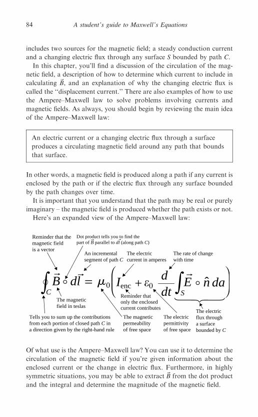
includes two sources for the magnetic field; a steady conduction current

and a changing electric flux through any surface S bounded by path C.

In this chapter, you’ll find a discussion of the circulation of the mag-

netic field, a description of how to determine which current to include in

calculating ~B, and an explanation of why the changing electric flux is

called the ‘‘displacement current.’’ There are also examples of how to use

the Ampere–Maxwell law to solve problems involving currents and

magnetic fields. As always, you should begin by reviewing the main idea

of the Ampere–Maxwell law:

An electric current or a changing electric flux through a surface

produces a circulating magnetic field around any path that bounds

that surface.

In other words, a magnetic field is produced along a path if any current is

enclosed by the path or if the electric flux through any surface bounded

by the path changes over time.

It is important that you understand that the path may be real or purely

imaginary – the magnetic field is produced whether the path exists or not.

Here’s an expanded view of the Ampere–Maxwell law:

Of what use is the Ampere–Maxwell law? You can use it to determine the

circulation of the magnetic field if you’re given information about the

enclosed current or the change in electric flux. Furthermore, in highly

symmetric situations, you may be able to extract ~B from the dot product

and the integral and determine the magnitude of the magnetic field.

C

dlB =∫ ∫0 Ienc +�0ddt S

E ˆ dan

Tells you to sum up the contributionsfrom each portion of closed path C ina direction given by the right-hand rule

The magneticfield in teslas

Dot product tells you to find thepart of B parallel to dl (along path C)

Reminder that themagnetic fieldis a vector

An incrementalsegment of path C

The magneticpermeabilityof free space

The electric current in amperes

Reminder thatonly the enclosedcurrent contributes

The electricpermittivityof free space

The electric flux througha surfacebounded by C

The rate of changewith time


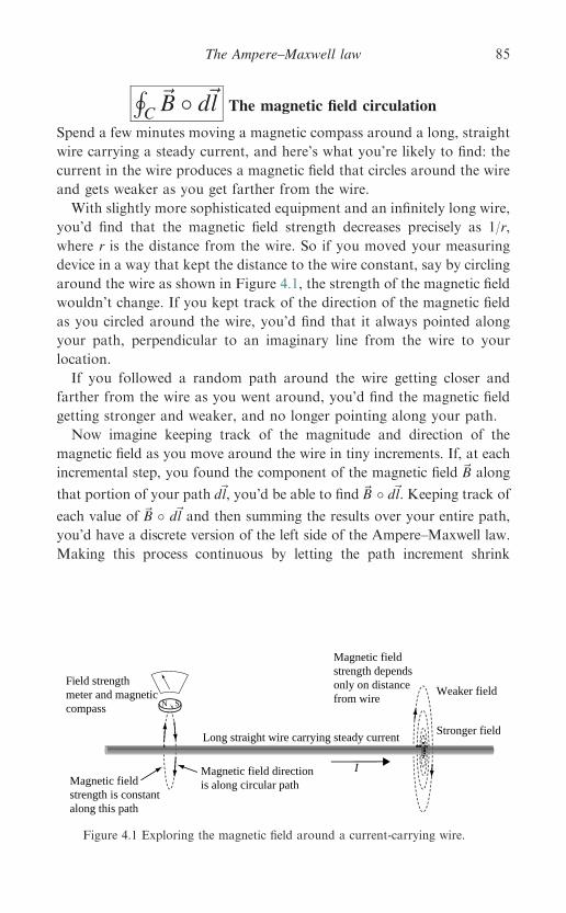
HC~B � d~l The magnetic field circulation

Spend a few minutes moving a magnetic compass around a long, straight

wire carrying a steady current, and here’s what you’re likely to find: the

current in the wire produces a magnetic field that circles around the wire

and gets weaker as you get farther from the wire.

With slightly more sophisticated equipment and an infinitely long wire,

you’d find that the magnetic field strength decreases precisely as 1/r,

where r is the distance from the wire. So if you moved your measuring

device in a way that kept the distance to the wire constant, say by circling

around the wire as shown in Figure 4.1, the strength of the magnetic field

wouldn’t change. If you kept track of the direction of the magnetic field

as you circled around the wire, you’d find that it always pointed along

your path, perpendicular to an imaginary line from the wire to your

location.

If you followed a random path around the wire getting closer and

farther from the wire as you went around, you’d find the magnetic field

getting stronger and weaker, and no longer pointing along your path.

Now imagine keeping track of the magnitude and direction of the

magnetic field as you move around the wire in tiny increments. If, at each

incremental step, you found the component of the magnetic field ~B along

that portion of your path d~l, you’d be able to find~B � d~l. Keeping track of

each value of ~B � d~l and then summing the results over your entire path,

you’d have a discrete version of the left side of the Ampere–Maxwell law.

Making this process continuous by letting the path increment shrink

N S

Long straight wire carrying steady current

Field strengthmeter and magneticcompass

Magnetic field directionis along circular path

I

Magnetic fieldstrength dependsonly on distancefrom wire

Stronger field

Weaker field

Magnetic fieldstrength is constantalong this path

Figure 4.1 Exploring the magnetic field around a current-carrying wire.

The Ampere–Maxwell law 85

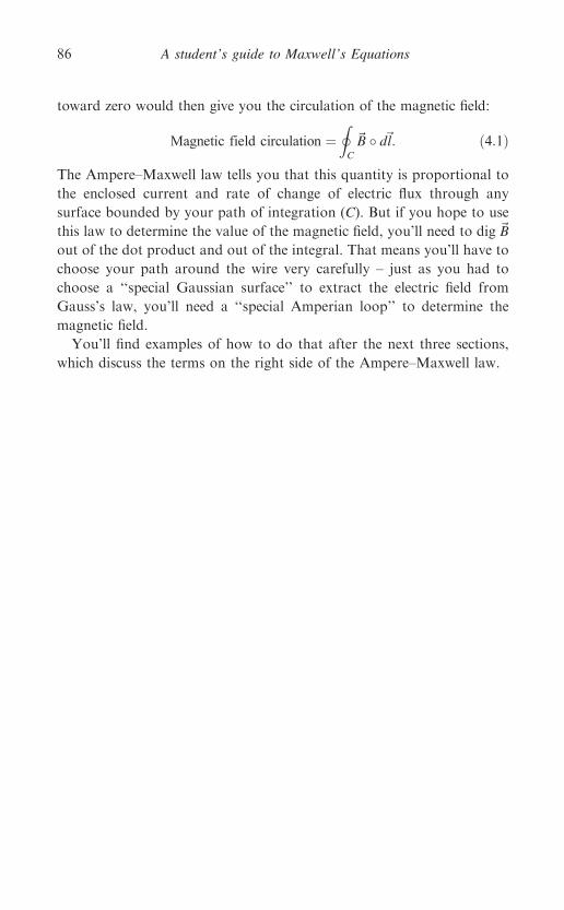
toward zero would then give you the circulation of the magnetic field:

Magnetic field circulation ¼IC

~B � d~l: ð4:1Þ

The Ampere–Maxwell law tells you that this quantity is proportional to

the enclosed current and rate of change of electric flux through any

surface bounded by your path of integration (C). But if you hope to use

this law to determine the value of the magnetic field, you’ll need to dig ~B

out of the dot product and out of the integral. That means you’ll have to

choose your path around the wire very carefully – just as you had to

choose a ‘‘special Gaussian surface’’ to extract the electric field from

Gauss’s law, you’ll need a ‘‘special Amperian loop’’ to determine the

magnetic field.

You’ll find examples of how to do that after the next three sections,

which discuss the terms on the right side of the Ampere–Maxwell law.


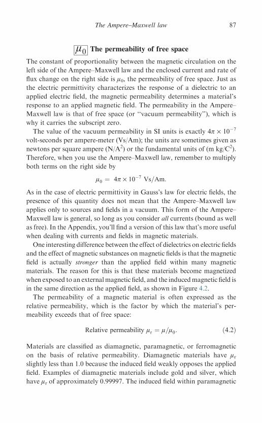
l0 The permeability of free space

The constant of proportionality between the magnetic circulation on the

left side of the Ampere–Maxwell law and the enclosed current and rate of

flux change on the right side is l0, the permeability of free space. Just as

the electric permittivity characterizes the response of a dielectric to an

applied electric field, the magnetic permeability determines a material’s

response to an applied magnetic field. The permeability in the Ampere–

Maxwell law is that of free space (or ‘‘vacuum permeability’’), which is

why it carries the subscript zero.

The value of the vacuum permeability in SI units is exactly 4p · 10�7

volt-seconds per ampere-meter (Vs/Am); the units are sometimes given as

newtons per square ampere (N/A2) or the fundamental units of (m kg/C2).

Therefore, when you use the Ampere–Maxwell law, remember to multiply

both terms on the right side by

l0 ¼ 4p · 10�7 Vs=Am:

As in the case of electric permittivity in Gauss’s law for electric fields, the

presence of this quantity does not mean that the Ampere–Maxwell law

applies only to sources and fields in a vacuum. This form of the Ampere–

Maxwell law is general, so long as you consider all currents (bound as well

as free). In the Appendix, you’ll find a version of this law that’s more useful

when dealing with currents and fields in magnetic materials.

One interesting difference between the effect of dielectrics on electric fields

and the effect of magnetic substances on magnetic fields is that the magnetic

field is actually stronger than the applied field within many magnetic

materials. The reason for this is that these materials become magnetized

when exposed to an externalmagnetic field, and the inducedmagnetic field is

in the same direction as the applied field, as shown in Figure 4.2.

The permeability of a magnetic material is often expressed as the

relative permeability, which is the factor by which the material’s per-

meability exceeds that of free space:

Relative permeability lr ¼ l=l0: ð4:2Þ

Materials are classified as diamagnetic, paramagnetic, or ferromagnetic

on the basis of relative permeability. Diamagnetic materials have lrslightly less than 1.0 because the induced field weakly opposes the applied

field. Examples of diamagnetic materials include gold and silver, which

have lr of approximately 0.99997. The induced field within paramagnetic


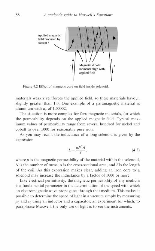
materials weakly reinforces the applied field, so these materials have lrslightly greater than 1.0. One example of a paramagnetic material is

aluminum with lr of 1.00002.The situation is more complex for ferromagnetic materials, for which

the permeability depends on the applied magnetic field. Typical max-

imum values of permeability range from several hundred for nickel and

cobalt to over 5000 for reasonably pure iron.

As you may recall, the inductance of a long solenoid is given by the

expression

L ¼ lN2A

‘; ð4:3Þ

where l is the magnetic permeability of the material within the solenoid,

N is the number of turns, A is the cross-sectional area, and ‘ is the length

of the coil. As this expression makes clear, adding an iron core to a

solenoid may increase the inductance by a factor of 5000 or more.

Like electrical permittivity, the magnetic permeability of any medium

is a fundamental parameter in the determination of the speed with which

an electromagnetic wave propagates through that medium. This makes it

possible to determine the speed of light in a vacuum simply by measuring

l0 and e0 using an inductor and a capacitor; an experiment for which, to

paraphrase Maxwell, the only use of light is to see the instruments.

Magnetic dipolemoments align withapplied field

Applied magneticfield produced bycurrent I

I I

Figure 4.2 Effect of magnetic core on field inside solenoid.


Ienc The enclosed electric current

Although the concept of ‘‘enclosed current’’ sounds simple, the question

of exactly which current to include on the right side of the Ampere–

Maxwell law requires careful consideration.

It should be clear from the first section of this chapter that the

‘‘enclosing’’ is done by the path C around which the magnetic field is

integrated (if you’re having trouble imagining a path enclosing anything,

perhaps ‘‘encircling’’ is a better word). However, consider for a moment

the paths and currents shown in Figure 4.3; which of the currents are

enclosed by paths C1, C2, and C3, and which are not?

The easiest way to answer that question is to imagine a membrane

stretched across the path, as shown in Figure 4.4. The enclosed current is

then just the net current that penetrates the membrane.

The reason for saying ‘‘net’’ current is that the direction of the current

relative to the direction of integration must be considered. By convention,

the right-hand rule determines whether a current is counted as positive or

negative: if you wrap the fingers of your right hand around the path in the

(a) (b) (c)

C1I1I2 C2 I3

C3

Figure 4.3 Currents enclosed (and not enclosed) by paths.

I1

C1

I2

C2 C3

I3

(a) (b) (c)

Figure 4.4 Membranes stretched across paths.


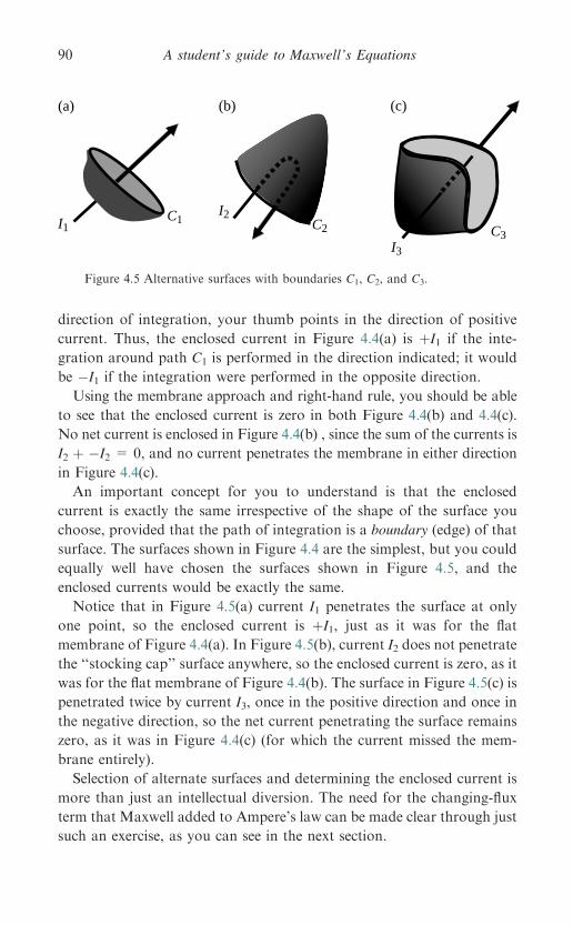
direction of integration, your thumb points in the direction of positive

current. Thus, the enclosed current in Figure 4.4(a) is þI1 if the inte-

gration around path C1 is performed in the direction indicated; it would

be �I1 if the integration were performed in the opposite direction.

Using the membrane approach and right-hand rule, you should be able

to see that the enclosed current is zero in both Figure 4.4(b) and 4.4(c).

No net current is enclosed in Figure 4.4(b) , since the sum of the currents is

I2 þ �I2 = 0, and no current penetrates the membrane in either direction

in Figure 4.4(c).

An important concept for you to understand is that the enclosed

current is exactly the same irrespective of the shape of the surface you

choose, provided that the path of integration is a boundary (edge) of that

surface. The surfaces shown in Figure 4.4 are the simplest, but you could

equally well have chosen the surfaces shown in Figure 4.5, and the

enclosed currents would be exactly the same.

Notice that in Figure 4.5(a) current I1 penetrates the surface at only

one point, so the enclosed current is þI1, just as it was for the flat

membrane of Figure 4.4(a). In Figure 4.5(b), current I2 does not penetrate

the ‘‘stocking cap’’ surface anywhere, so the enclosed current is zero, as it

was for the flat membrane of Figure 4.4(b). The surface in Figure 4.5(c) is

penetrated twice by current I3, once in the positive direction and once in

the negative direction, so the net current penetrating the surface remains

zero, as it was in Figure 4.4(c) (for which the current missed the mem-

brane entirely).

Selection of alternate surfaces and determining the enclosed current is

more than just an intellectual diversion. The need for the changing-flux

term that Maxwell added to Ampere’s law can be made clear through just

such an exercise, as you can see in the next section.

I1C1 I2

C2 C3 I3

(a) (b) (c)

Figure 4.5 Alternative surfaces with boundaries C1, C2, and C3.


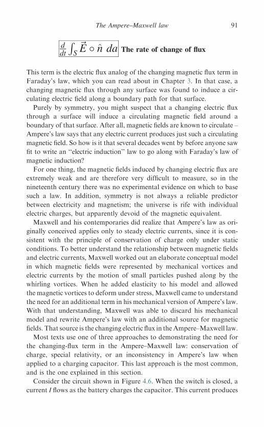
ddt

RS~E � n da The rate of change of flux

This term is the electric flux analog of the changing magnetic flux term in

Faraday’s law, which you can read about in Chapter 3. In that case, a

changing magnetic flux through any surface was found to induce a cir-

culating electric field along a boundary path for that surface.

Purely by symmetry, you might suspect that a changing electric flux

through a surface will induce a circulating magnetic field around a

boundary of that surface. After all, magnetic fields are known to circulate –

Ampere’s law says that any electric current produces just such a circulating

magnetic field. So how is it that several decades went by before anyone saw

fit to write an ‘‘electric induction’’ law to go along with Faraday’s law of

magnetic induction?

For one thing, the magnetic fields induced by changing electric flux are

extremely weak and are therefore very difficult to measure, so in the

nineteenth century there was no experimental evidence on which to base

such a law. In addition, symmetry is not always a reliable predictor

between electricity and magnetism; the universe is rife with individual

electric charges, but apparently devoid of the magnetic equivalent.

Maxwell and his contemporaries did realize that Ampere’s law as ori-

ginally conceived applies only to steady electric currents, since it is con-

sistent with the principle of conservation of charge only under static

conditions. To better understand the relationship between magnetic fields

and electric currents, Maxwell worked out an elaborate conceptual model

in which magnetic fields were represented by mechanical vortices and

electric currents by the motion of small particles pushed along by the

whirling vortices. When he added elasticity to his model and allowed

the magnetic vortices to deform under stress, Maxwell came to understand

the need for an additional term in his mechanical version of Ampere’s law.

With that understanding, Maxwell was able to discard his mechanical

model and rewrite Ampere’s law with an additional source for magnetic

fields. That source is the changing electric flux in theAmpere–Maxwell law.

Most texts use one of three approaches to demonstrating the need for

the changing-flux term in the Ampere–Maxwell law: conservation of

charge, special relativity, or an inconsistency in Ampere’s law when

applied to a charging capacitor. This last approach is the most common,

and is the one explained in this section.

Consider the circuit shown in Figure 4.6. When the switch is closed, a

current I flows as the battery charges the capacitor. This current produces


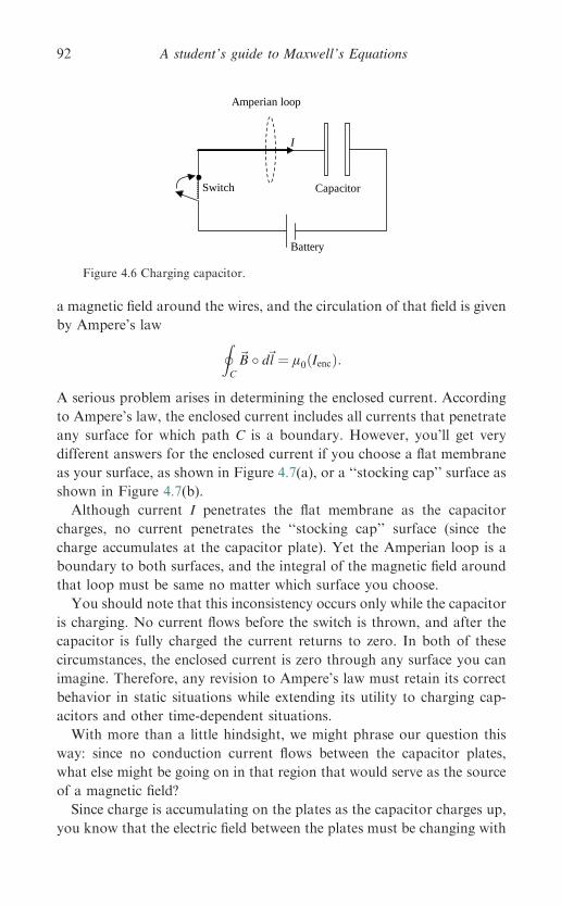
a magnetic field around the wires, and the circulation of that field is given

by Ampere’s law IC

~B � d~l ¼ l0 Iencð Þ:

A serious problem arises in determining the enclosed current. According

to Ampere’s law, the enclosed current includes all currents that penetrate

any surface for which path C is a boundary. However, you’ll get very

different answers for the enclosed current if you choose a flat membrane

as your surface, as shown in Figure 4.7(a), or a ‘‘stocking cap’’ surface as

shown in Figure 4.7(b).

Although current I penetrates the flat membrane as the capacitor

charges, no current penetrates the ‘‘stocking cap’’ surface (since the

charge accumulates at the capacitor plate). Yet the Amperian loop is a

boundary to both surfaces, and the integral of the magnetic field around

that loop must be same no matter which surface you choose.

You should note that this inconsistency occurs only while the capacitor

is charging. No current flows before the switch is thrown, and after the

capacitor is fully charged the current returns to zero. In both of these

circumstances, the enclosed current is zero through any surface you can

imagine. Therefore, any revision to Ampere’s law must retain its correct

behavior in static situations while extending its utility to charging cap-

acitors and other time-dependent situations.

With more than a little hindsight, we might phrase our question this

way: since no conduction current flows between the capacitor plates,

what else might be going on in that region that would serve as the source

of a magnetic field?

Since charge is accumulating on the plates as the capacitor charges up,

you know that the electric field between the plates must be changing with

I

Battery

Capacitor

Amperian loop

Switch

Figure 4.6 Charging capacitor.


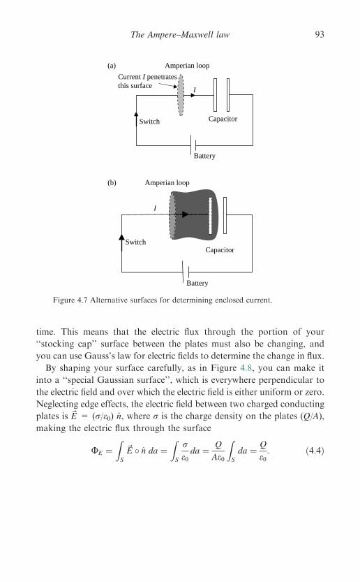
time. This means that the electric flux through the portion of your

‘‘stocking cap’’ surface between the plates must also be changing, and

you can use Gauss’s law for electric fields to determine the change in flux.

By shaping your surface carefully, as in Figure 4.8, you can make it

into a ‘‘special Gaussian surface’’, which is everywhere perpendicular to

the electric field and over which the electric field is either uniform or zero.

Neglecting edge effects, the electric field between two charged conducting

plates is ~E = (r/e0) n, where r is the charge density on the plates (Q/A),

making the electric flux through the surface

UE ¼ZS

~E � n da ¼ZS

re0da ¼ Q

Ae0

ZS

da ¼ Q

e0: ð4:4Þ

Current I penetratesthis surface

I

Battery

Capacitor

Amperian loop(a)

Switch

Amperian loop(b)

Battery

Capacitor Switch

I

Figure 4.7 Alternative surfaces for determining enclosed current.


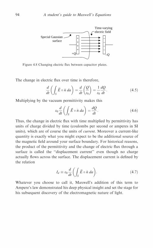
The change in electric flux over time is therefore,

d

dt

ZS

~E � n da

� �¼ d

dt

Q

e0

� �¼ 1

e0

dQ

dt: ð4:5Þ

Multiplying by the vacuum permittivity makes this

e0d

dt

ZS

~E � n da

� �¼ dQ

dt: ð4:6Þ

Thus, the change in electric flux with time multiplied by permittivity has

units of charge divided by time (coulombs per second or amperes in SI

units), which are of course the units of current. Moreover a current-like

quantity is exactly what you might expect to be the additional source of

the magnetic field around your surface boundary. For historical reasons,

the product of the permittivity and the change of electric flux through a

surface is called the ‘‘displacement current’’ even though no charge

actually flows across the surface. The displacement current is defined by

the relation

Id � e0d

dt

ZS

~E � n da

� �: ð4:7Þ

Whatever you choose to call it, Maxwell’s addition of this term to

Ampere’s law demonstrated his deep physical insight and set the stage for

his subsequent discovery of the electromagnetic nature of light.

+Q –Q

Special Gaussiansurface

Time-varyingelectric field

++++

––––

Figure 4.8 Changing electric flux between capacitor plates.


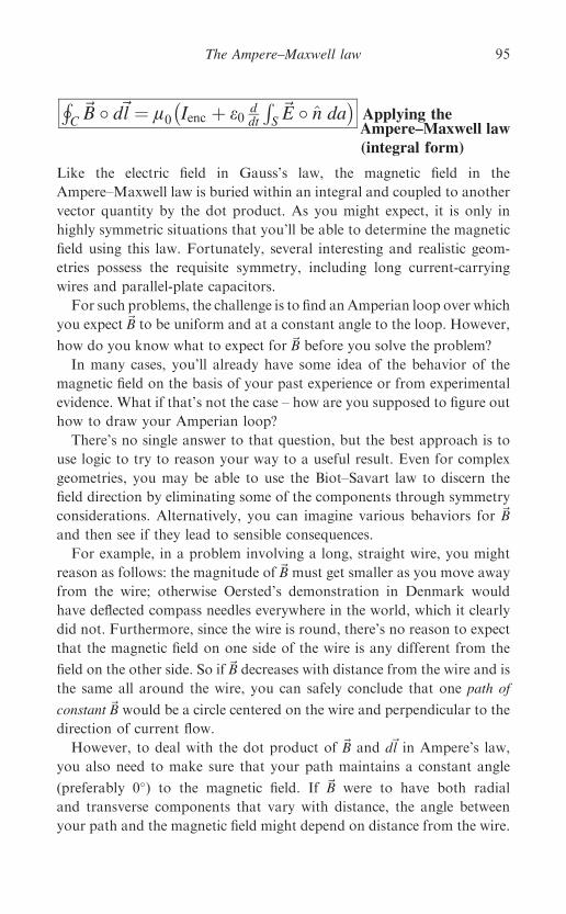
HC~B � d~l ¼ l0 Ienc þ e0 d

dt

RS~E � n da

� �Applying theAmpere–Maxwell law(integral form)

Like the electric field in Gauss’s law, the magnetic field in the

Ampere–Maxwell law is buried within an integral and coupled to another

vector quantity by the dot product. As you might expect, it is only in

highly symmetric situations that you’ll be able to determine the magnetic

field using this law. Fortunately, several interesting and realistic geom-

etries possess the requisite symmetry, including long current-carrying

wires and parallel-plate capacitors.

For such problems, the challenge is to find anAmperian loop over which

you expect~B to be uniform and at a constant angle to the loop. However,

how do you know what to expect for ~B before you solve the problem?

In many cases, you’ll already have some idea of the behavior of the

magnetic field on the basis of your past experience or from experimental

evidence. What if that’s not the case – how are you supposed to figure out

how to draw your Amperian loop?

There’s no single answer to that question, but the best approach is to

use logic to try to reason your way to a useful result. Even for complex

geometries, you may be able to use the Biot–Savart law to discern the

field direction by eliminating some of the components through symmetry

considerations. Alternatively, you can imagine various behaviors for ~B

and then see if they lead to sensible consequences.

For example, in a problem involving a long, straight wire, you might

reason as follows: the magnitude of~B must get smaller as you move away

from the wire; otherwise Oersted’s demonstration in Denmark would

have deflected compass needles everywhere in the world, which it clearly

did not. Furthermore, since the wire is round, there’s no reason to expect

that the magnetic field on one side of the wire is any different from the

field on the other side. So if~B decreases with distance from the wire and is

the same all around the wire, you can safely conclude that one path of

constant~B would be a circle centered on the wire and perpendicular to the

direction of current flow.

However, to deal with the dot product of ~B and d~l in Ampere’s law,

you also need to make sure that your path maintains a constant angle

(preferably 0�) to the magnetic field. If ~B were to have both radial

and transverse components that vary with distance, the angle between

your path and the magnetic field might depend on distance from the wire.


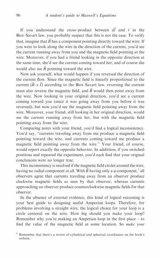
If you understand the cross–product between d~l and r in the

Biot–Savart law, you probably suspect that this is not the case. To verify

that, imagine that~B has a component pointing directly toward the wire. If

you were to look along the wire in the direction of the current, you’d see

the current running away from you and the magnetic field pointing at the

wire. Moreover, if you had a friend looking in the opposite direction at

the same time, she’d see the current coming toward her, and of course she

would also see ~B pointing toward the wire.

Now ask yourself, what would happen if you reversed the direction of

the current flow. Since the magnetic field is linearly proportional to the

current (~B /~I) according to the Biot–Savart law, reversing the current

must also reverse the magnetic field, and ~B would then point away from

the wire. Now looking in your original direction, you’d see a current

coming toward you (since it was going away from you before it was

reversed), but now you’d see the magnetic field pointing away from the

wire. Moreover, your friend, still looking in her original direction, would

see the current running away from her, but with the magnetic field

pointing away from the wire.

Comparing notes with your friend, you’d find a logical inconsistency.

You’d say, ‘‘currents traveling away from me produce a magnetic field

pointing toward the wire, and currents coming toward me produce a

magnetic field pointing away from the wire.’’ Your friend, of course,

would report exactly the opposite behavior. In addittion, if you switched

positions and repeated the experiment, you’d each find that your original

conclusions were no longer true.

This inconsistency is resolved if the magnetic field circles around the wire,

having no radial component at all. With~B having only a u-component,5 all

observers agree that currents traveling away from an observer produce

clockwise magnetic fields as seen by that observer, whereas currents

approaching an observer produce counterclockwise magnetic fields for that

observer.

In the absence of external evidence, this kind of logical reasoning is

your best guide to designing useful Amperian loops. Therefore, for

problems involving a straight wire, the logical choice for your loop is a

circle centered on the wire. How big should you make your loop?

Remember why you’re making an Amperian loop in the first place – to

find the value of the magnetic field at some location. So make your

5 Remember that there’s a review of cylindrical and spherical coordinates on the book’swebsite.


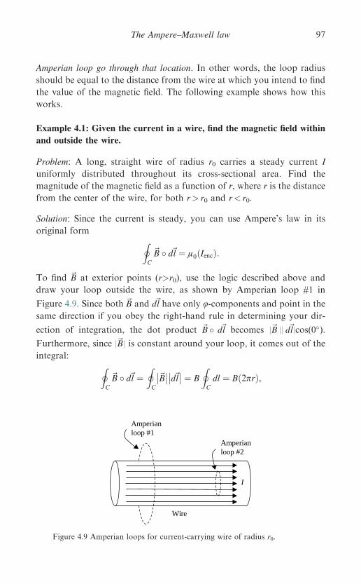
Amperian loop go through that location. In other words, the loop radius

should be equal to the distance from the wire at which you intend to find

the value of the magnetic field. The following example shows how this

works.

Example 4.1: Given the current in a wire, find the magnetic field within

and outside the wire.

Problem: A long, straight wire of radius r0 carries a steady current I

uniformly distributed throughout its cross-sectional area. Find the

magnitude of the magnetic field as a function of r, where r is the distance

from the center of the wire, for both r> r0 and r< r0.

Solution: Since the current is steady, you can use Ampere’s law in its

original form IC

~B � d~l ¼ l0 Iencð Þ:

To find ~B at exterior points (r>r0), use the logic described above and

draw your loop outside the wire, as shown by Amperian loop #1 in

Figure 4.9. Since both ~B and d~l have only u-components and point in the

same direction if you obey the right-hand rule in determining your dir-

ection of integration, the dot product ~B � d~l becomes |~B || d~l|cos(0�).Furthermore, since |~B| is constant around your loop, it comes out of the

integral: IC

~B � d~l ¼IC

~B d~l ¼ B

IC

dl ¼ Bð2prÞ,

Amperianloop #1

Wire

I

Amperianloop #2

Figure 4.9 Amperian loops for current-carrying wire of radius r0.


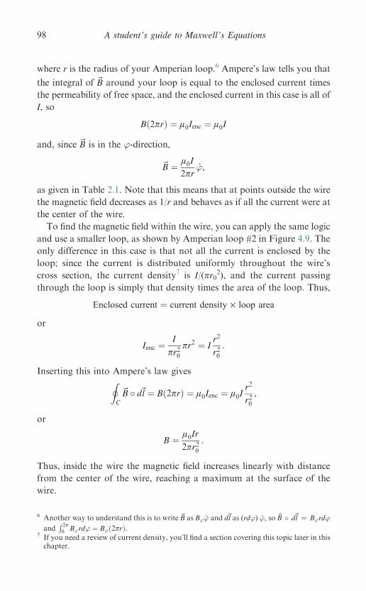
where r is the radius of your Amperian loop.6 Ampere’s law tells you that

the integral of ~B around your loop is equal to the enclosed current times

the permeability of free space, and the enclosed current in this case is all of

I, so

Bð2prÞ ¼ l0Ienc ¼ l0I

and, since ~B is in the ’-direction,

~B ¼ l0I2pr

’,

as given in Table 2.1. Note that this means that at points outside the wire

the magnetic field decreases as 1/r and behaves as if all the current were at

the center of the wire.

To find the magnetic field within the wire, you can apply the same logic

and use a smaller loop, as shown by Amperian loop #2 in Figure 4.9. The

only difference in this case is that not all the current is enclosed by the

loop; since the current is distributed uniformly throughout the wire’s

cross section, the current density7 is I/(pr02), and the current passing

through the loop is simply that density times the area of the loop. Thus,

Enclosed current ¼ current density · loop area

or

Ienc ¼ I

pr20pr2 ¼ I

r2

r20:

Inserting this into Ampere’s law givesIC

~B � d~l ¼ Bð2prÞ ¼ l0Ienc ¼ l0Ir2

r20,

or

B ¼ l0Ir

2pr20:

Thus, inside the wire the magnetic field increases linearly with distance

from the center of the wire, reaching a maximum at the surface of the

wire.

6 Another way to understand this is to write~B as B’’ and d~l as (rd’) ’, so~B � d~l ¼ B’rd’

andR 2p0 B’rd’ ¼ B’ð2prÞ.

7 If you need a review of current density, you’ll find a section covering this topic later in thischapter.


Example 4.2: Given the time-dependent charge on a capacitor, find the

rate of change of the electric flux between the plates and the magnitude

of the resulting magnetic field at a specified location.

Problem: A battery with potential difference DV charges a circular

parallel-plate capacitor of capacitance C and plate radius r0 through a

wire with resistance R. Find the rate of change of the electric flux between

the plates as a function of time and the magnetic field at a distance r from

the center of the plates.

Solution: From Equation 4.5, the rate of change of electric flux between

the plates is

dUE

dt¼ d

dt

ZS

~E � n da

0@

1A ¼ 1

e0

dQ

dt,

where Q is the total charge on each plate. So you should begin by

determining how the charge on a capacitor plate changes with time as the

capacitor is charged. If you’ve studied series RC circuits, you may recall

that the relevant expression is

QðtÞ ¼ CDVð1� e�t=RCÞ,

where DV, R, and C represent the potential difference, the series resist-

ance, and the capacitance, respectively. Thus,

dUE

dt¼ 1

e0

d

dtCDVð1� e�t=RCÞh i

¼ 1

e0CDV

1

RCe�t=RC

� �¼ DV

e0Re�t=RC :

This is the rate of change of the total electric flux between the plates. To

find the magnetic field at a distance r from the center of the plates, you’re

going to have to construct a special Amperian loop to help you extract

the magnetic field from the integral in the Ampere–Maxwell law:

IC


dt

ZS

~E � n da

� �:

Since no charge flows between the capacitor plates, Ienc=0, and

IC

~B � d~l ¼ l0 e0d

dt

ZS

~E � n da

� �:


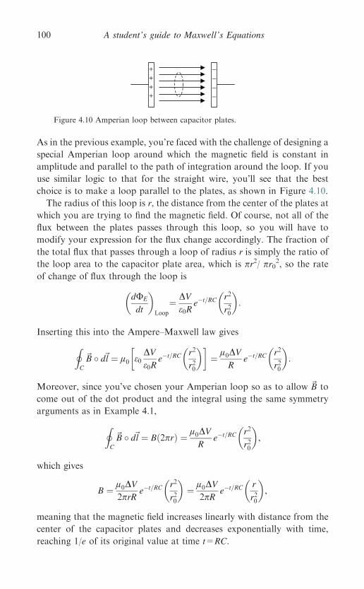
As in the previous example, you’re faced with the challenge of designing a

special Amperian loop around which the magnetic field is constant in

amplitude and parallel to the path of integration around the loop. If you

use similar logic to that for the straight wire, you’ll see that the best

choice is to make a loop parallel to the plates, as shown in Figure 4.10.

The radius of this loop is r, the distance from the center of the plates at

which you are trying to find the magnetic field. Of course, not all of the

flux between the plates passes through this loop, so you will have to

modify your expression for the flux change accordingly. The fraction of

the total flux that passes through a loop of radius r is simply the ratio of

the loop area to the capacitor plate area, which is pr2/ pr02, so the rate

of change of flux through the loop is

dUE

dt

� �Loop

¼ DV

e0Re�t=RC r2

r20

� �:

Inserting this into the Ampere–Maxwell law givesIC

~B � d~l ¼ l0 e0DV

e0Re�t=RC r2

r20

� �� ¼ l0DV

Re�t=RC r2

r20

� �:

Moreover, since you’ve chosen your Amperian loop so as to allow ~B to

come out of the dot product and the integral using the same symmetry

arguments as in Example 4.1,IC

~B � d~l ¼ Bð2prÞ ¼ l0DVR

e�t=RC r2

r20

� �,

which gives

B ¼ l0DV2prR

e�t=RC r2

r20

� �¼ l0DV

2pRe�t=RC r

r20

� �,

meaning that the magnetic field increases linearly with distance from the

center of the capacitor plates and decreases exponentially with time,

reaching 1/e of its original value at time t=RC.

++++

––––

Figure 4.10 Amperian loop between capacitor plates.


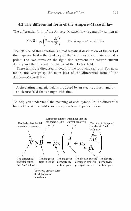
4.2 The differential form of the Ampere–Maxwell law

The differential form of the Ampere–Maxwell law is generally written as

~r ·~B ¼ l0 ~J þ e0@~E

@t

!The Ampere–Maxwell law:

The left side of this equation is a mathematical description of the curl of

the magnetic field – the tendency of the field lines to circulate around a

point. The two terms on the right side represent the electric current

density and the time rate of change of the electric field.

These terms are discussed in detail in the following sections. For now,

make sure you grasp the main idea of the differential form of the

Ampere–Maxwell law:

A circulating magnetic field is produced by an electric current and by

an electric field that changes with time.


form of the Ampere–Maxwell law, here’s an expanded view:

B J�× = + �E�t

0 �0

Reminder that the deloperator is a vector

Reminder that themagnetic field is a vector

Reminder that thecurrent density is a vector

The rate of change of the electric fieldwith time


The electric currentdensity in amperesper square meter


The magneticfield in teslas

The differentialoperator called“del” or “nabla”

The cross-product turnsthe del operatorinto the curl


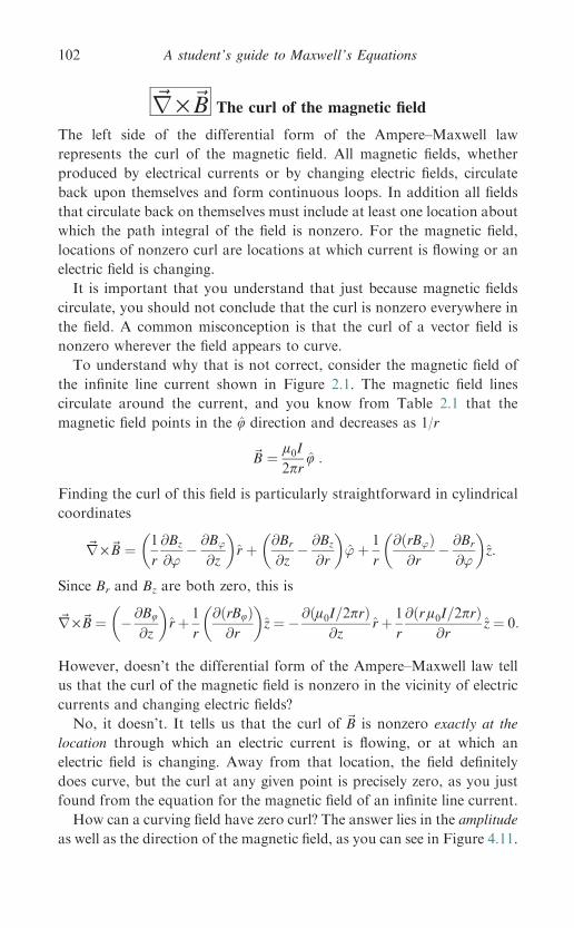
~r·~B The curl of the magnetic field

The left side of the differential form of the Ampere–Maxwell law

represents the curl of the magnetic field. All magnetic fields, whether

produced by electrical currents or by changing electric fields, circulate

back upon themselves and form continuous loops. In addition all fields

that circulate back on themselves must include at least one location about

which the path integral of the field is nonzero. For the magnetic field,

locations of nonzero curl are locations at which current is flowing or an

electric field is changing.

It is important that you understand that just because magnetic fields

circulate, you should not conclude that the curl is nonzero everywhere in

the field. A common misconception is that the curl of a vector field is

nonzero wherever the field appears to curve.

To understand why that is not correct, consider the magnetic field of

the infinit e line current shown in Figure 2. 1. The magnet ic fie ld lines

circulate around the current, and you know from Table 2.1 that the

magnetic field points in the u direction and decreases as 1/r

~B ¼ l0I2pr

u :

Finding the curl of this field is particularly straightforward in cylindrical

coordinates

~r ·~B ¼ 1

r

@Bz

@’� @B’

@z

� �r þ @Br

@z� @Bz

@r

� �’þ 1

r

@ðrB’Þ@r

� @Br

@’

� �z:

Since Br and Bz are both zero, this is

~r·~B ¼ �@Bu

@z

� �rþ 1

r

@ðrBuÞ@r

� �z ¼ �@ l0I=2prð Þ

@zrþ 1

r

@ r l0I=2prð Þ@r

z ¼ 0:

However, doesn’t the differential form of the Ampere–Maxwell law tell

us that the curl of the magnetic field is nonzero in the vicinity of electric

currents and changing electric fields?

No, it doesn’t. It tells us that the curl of ~B is nonzero exactly at the

location through which an electric current is flowing, or at which an

electric field is changing. Away from that location, the field definitely

does curve, but the curl at any given point is precisely zero, as you just

found from the equation for the magnetic field of an infinite line current.

How can a curving field have zero curl? The answer lies in the amplitude

as well as the direction of the magnetic field, as you can see in Figure 4.11.


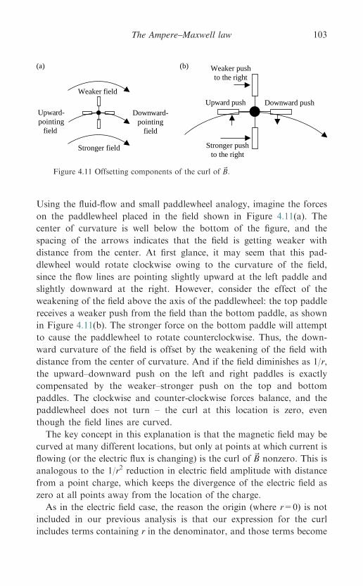
Using the fluid-flow and small paddlewheel analogy, imagine the forces

on the paddlewheel placed in the field shown in Figure 4.11(a). The

center of curvature is well below the bottom of the figure, and the

spacing of the arrows indicates that the field is getting weaker with

distance from the center. At first glance, it may seem that this pad-

dlewheel would rotate clockwise owing to the curvature of the field,

since the flow lines are pointing slightly upward at the left paddle and

slightly downward at the right. However, consider the effect of the

weakening of the field above the axis of the paddlewheel: the top paddle

receives a weaker push from the field than the bottom paddle, as shown

in Figure 4.11(b). The stronger force on the bottom paddle will attempt

to cause the paddlewheel to rotate counterclockwise. Thus, the down-

ward curvature of the field is offset by the weakening of the field with

distance from the center of curvature. And if the field diminishes as 1/r,

the upward–downward push on the left and right paddles is exactly

compensated by the weaker–stronger push on the top and bottom

paddles. The clockwise and counter-clockwise forces balance, and the

paddlewheel does not turn – the curl at this location is zero, even

though the field lines are curved.

The key concept in this explanation is that the magnetic field may be

curved at many different locations, but only at points at which current is

flowing (or the electric flux is changing) is the curl of ~B nonzero. This is

analogous to the 1/r2 reduction in electric field amplitude with distance

from a point charge, which keeps the divergence of the electric field as

zero at all points away from the location of the charge.

As in the electric field case, the reason the origin (where r=0) is not

included in our previous analysis is that our expression for the curl

includes terms containing r in the denominator, and those terms become

Weaker field

Stronger field

Upward-pointing

field

Downward-pointing

field

Weaker pushto the right

Stronger pushto the right

Upward push Downward push

(a) (b)

Figure 4.11 Offsetting components of the curl of ~B:


infinite at the origin. To evaluate the curl at the origin, use the formal

definition of curl as described in Chapter 3:

~r ·~B � limDS!0

1

DS

IC

~B � d~l

Considering a special Amperian loop surrounding the current, this is

~r ·~B � limDS!0

1

DS

IC

~B � d~l ¼ limDS!0

1

DS

l0~I2pr

ð2prÞ !

¼ limDS!0

1

DSl0~I

� �:

However,~I=DS is just the average current density over the surface DS, and

as DS shrinks to zero, this becomes equal to~J, the current density at the

origin. Thus, at the origin

~r ·~B ¼ l0~J

in accordance with Ampere’s law.

So just as you might be fooled into thinking that charge-based electric

field vectors ‘‘diverge’’ everywhere because they get farther apart, you

might also think that magnetic field vectors have curl everywhere because

they curve around a central point. But the key factor in determining the

curl at any point is not simply the curvature of the field lines at that

point, but how the change in the field from one side of the point to the

other (say from left to right) compares to the change in the field in the

orthogonal direction (below to above). If those spatial derivatives

are precisely equal, then the curl is zero at that point.

In the case of a current-carrying wire, the reduction in the amplitude of

the magnetic field away from the wire exactly compensates for the

curvature of the field lines. Thus, the curl of the magnetic field is zero

everywhere except at the wire itself, where electric current is flowing.


~J The electric current density

The right side of the differential form of the Ampere–Maxwell law

contains two source terms for the circulating magnetic field; the first

involves the vector electric current density. This is sometimes called

the ‘‘volume current density,’’ which can be a source of confusion if

you’re accustomed to ‘‘volume density’’ meaning the amount of

something per unit volume, such as kg/m3 for mass density or C/m3

for charge density.

This is not the case for current density, which is defined as the vector

current flowing through a unit cross-sectional area perpendicular to the

direction of the current. Thus, the units of current density are not

amperes per cubic meter, but rather amperes per square meter (A/m2).

To understand the concept of current density, recall that in the dis-

cussion of flux in Chapter 1, the quantity ~A is defined as the number

density of the fluid (particles per cubic meter) times the velocity of the

flow (meters per second). As the product of the number density (a scalar)

and the velocity (a vector), ~A is a vector in the same direction as the

velocity, with units of particles per square meter per second. To find the

number of particles per second passing through a surface in the simplest

case (~A uniform and perpendicular to the surface), you simply multiply ~A

by the area of the surface.

These same concepts are relevant for current density, provided we

consider the amount of charge passing through the surface rather than the

number of atoms. If the number density of charge carriers is n and the

charge per carrier is q, then the amount of charge passing through a unit

area perpendicular to the flow per second is

~J ¼ nq~vd ðC=m2s or A=m2Þ; ð4:8Þ

where~vd is the average drift velocity of charge carriers. Thus, the direc-

tion of the current density is the direction of current flow, and the

magnitude is the current per unit area, as shown in Figure 4.12.

The complexity of the relationship between the total current I through

a surface and the current density ~J depends on the geometry of the

situation. If the current density ~J is uniform over a surface S and is

everywhere perpendicular to the surface, the relationship is

I ¼ ~J · ðsurface areaÞ ~J uniform and perpendicular to S: ð4:9Þ


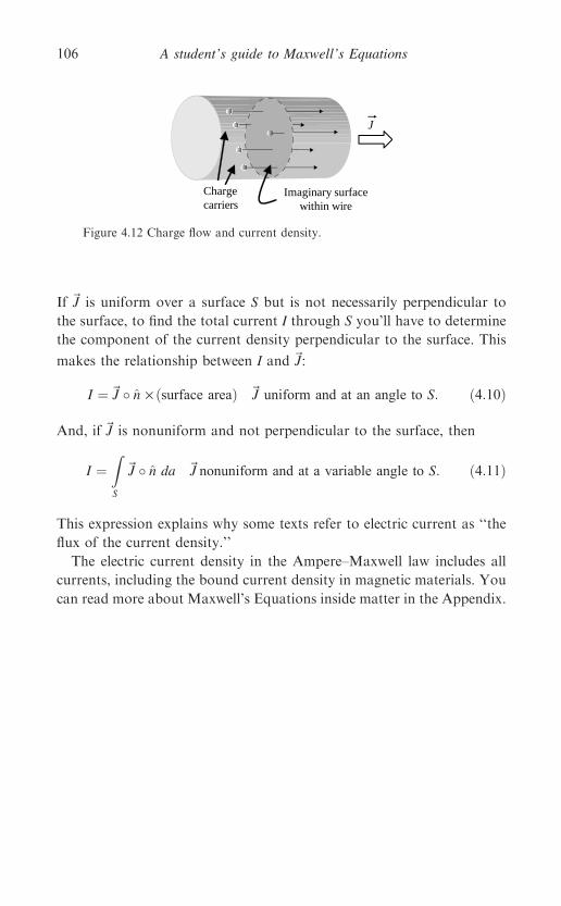
If ~J is uniform over a surface S but is not necessarily perpendicular to

the surface, to find the total current I through S you’ll have to determine

the component of the current density perpendicular to the surface. This

makes the relationship between I and ~J:

I ¼~J � n · ðsurface areaÞ ~J uniform and at an angle to S: ð4:10Þ

And, if ~J is nonuniform and not perpendicular to the surface, then

I ¼ZS

~J � n da ~J nonuniform and at a variable angle to S: ð4:11Þ

This expression explains why some texts refer to electric current as ‘‘the

flux of the current density.’’

The electric current density in the Ampere–Maxwell law includes all

currents, including the bound current density in magnetic materials. You

can read more about Maxwell’s Equations inside matter in the Appendix.

Imaginary surfacewithin wire

J

Chargecarriers

Figure 4.12 Charge flow and current density.


e0

@~E@t The displacement current density

The second source term for the magnetic field in the Ampere–Maxwell

law involves the rate of change of the electric field with time. When

multiplied by the electrical permittivity of free space, this term has SI

units of amperes per square meter. These units are identical to those of~J,

the conduction current density that also appears on the right side of the

differential form of the Ampere–Maxwell law. Maxwell originally

attributed this term to the physical displacement of electrical particles

caused by elastic deformation of magnetic vortices, and others coined the

term ‘‘displacement current’’ to describe the effect.

However, does the displacement current density represent an actual

current? Certainly not in the conventional sense of the word, since electric

current is defined as the physical movement of charge. But it is easy to

understand why a term that has units of amperes per square meter and

acts as a source of the magnetic field has retained that name over the

years. Furthermore, the displacement current density is a vector quantity

that has the same relationship to the magnetic field as does ~J, the con-

duction current density.

The key concept here is that a changing electric field produces a

changing magnetic field even when no charges are present and no phys-

ical current flows. Through this mechanism, electromagnetic waves may

propagate through even a perfect vacuum, as changing magnetic fields

induce electric fields, and changing electric fields induce magnetic fields.

The importance of the displacement current term, which arose initially

from Maxwell’s mechanical model, is difficult to overstate. Adding a

changing electric field as a source of the magnetic field certainly extended

the scope of Ampere’s law to time-dependent fields by eliminating the

inconsistency with the principle of conservation of charge. Far more

importantly, it allowed James Clerk Maxwell to establish a comprehen-

sive theory of electromagnetism, the first true field theory and the

foundation for much of twentieth century physics.


~r ·~B ¼ l0 ~J þ e0 @~E@t

� �Applying the Ampere–Maxwell

law (differential form)

The most common applications of the differential form of the Ampere–

Maxwell law are problems in which you’re provided with an expression

for the vector magnetic field and you’re asked to determine the electric

current density or the displacement current. Here are two examples of

this kind of problem.

Example 4.3: Given the magnetic field, find the current density at a

specified location.

Problem: Use the expressions for the magnetic field in Table 2.1 to find

the current density both inside and outside a long, straight wire of radius

r0 carrying current I uniformly throughout its volume in the positive

z-direction.

Solution: From Table 2.1 and Example 4.1, the magnetic field inside a

long, straight wire is

~B ¼ l0Ir

2pr20’,

where I is the current in the wire and r0 is the wire’s radius. In cylindrical

coordinates, the curl of ~B is

~r ·~B � 1

r

@Bz

@u� @Bu

@z

� �r þ @Br

@z� @Bz

@r

� �uþ 1

r

@ðrBuÞ@r

� @Br

@u

� �z:

And, since ~B has only a ’-component in this case,

~r ·~B � � @B’

@z

� �r þ 1

r

@ðrB’Þ@r

� �z ¼ 1

r

@�rð l0Ir=2pr20Þ

�@r

0@

1Az

¼ 1

r2r

l0I

2pr20

� �z ¼ l0I

pr20

� �z:

Using the static version of the Ampere–Maxwell law (since the current is

steady), you can find ~J from the curl of ~B:

~r · ~B ¼ l0 ~J� �

:


Thus,

~J ¼ 1

l0

l0I

pr20

� �z ¼ I

pr20z;

which is the current density within the wire. Taking the curl of the

expression for ~B outside the wire, you’ll find that ~J ¼ 0, as expected.

Example 4.4: Given the magnetic field, find the displacement current

density.

Problem: The expression for the magnetic field of a circular parallel-plate

capacitor found in Example 4.2 is

~B ¼ l0DV2pR

e�t=RC r

r20

� �’:

Use this result to find the displacement current density between the plates.

Solution: Once again you can use the curl of ~B in cylindrical coordinates:

~r ·~B � 1

r

@Bz

@’� @B’

@z

� �r þ @Br

@z� @Bz

@r

� �uþ 1

r

@ðrB’Þ@r

� @Br

@’

� �z:

And, once again ~B has only a ’-component:

~r ·~B ¼ � @B’

@z

� �r þ 1

r

@ðrB’Þ@r

� �z ¼ 1

r

@�ðrl0DV=2pRÞe�t=RC r

r20

� ��@r

24

35z

¼ 1

r2r

l0DV2pR

e�t=RC 1

r20

� �� z¼ l0DV

pRe�t=RC 1

r20

� �� z:

Since there is no conduction current between the plates,~J ¼ 0 in this case

and the Ampere–Maxwell law is

~r ·~B ¼ l0 e0@~E

@t

!;

from which you can find the displacement current density,

e0@~E

@t¼

~r ·~Bl0

¼ 1

l0

l0DVpR

e�t=RC 1

r20

� �� z ¼ DV

Re�t=RC 1

pr20

� z:

Problems

The following problems will test your understanding of the Ampere–

Maxwell law. Full solutions are available on the book’s website.


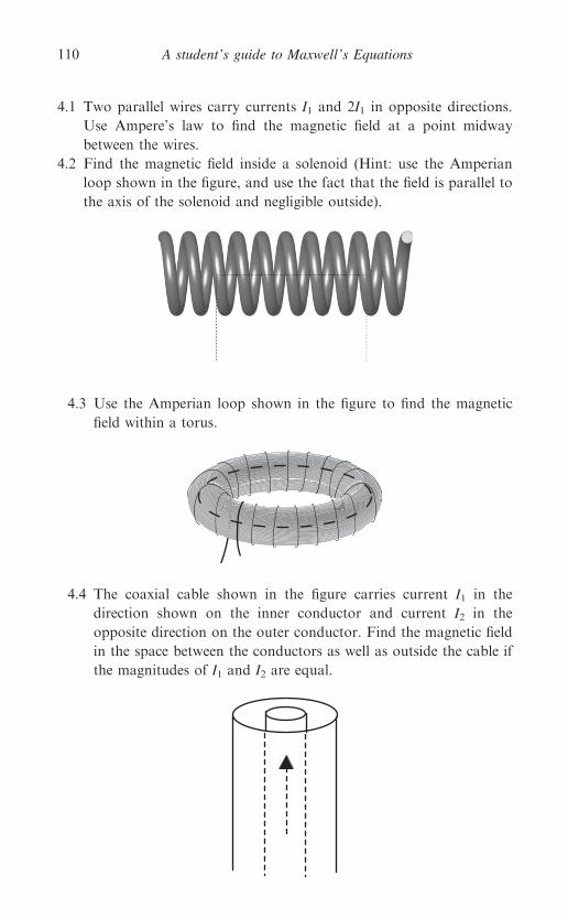
4.1 Two parallel wires carry currents I1 and 2I1 in opposite directions.

Use Ampere’s law to find the magnetic field at a point midway

between the wires.

4.2 Find the magnetic field inside a solenoid (Hint: use the Amperian

loop shown in the figure, and use the fact that the field is parallel to

the axis of the solenoid and negligible outside).

4.3 Use the Amperian loop shown in the figure to find the magnetic

field within a torus.

4.4 The coaxial cable shown in the figure carries current I1 in the

direction shown on the inner conductor and current I2 in the

opposite direction on the outer conductor. Find the magnetic field

in the space between the conductors as well as outside the cable if

the magnitudes of I1 and I2 are equal.


4.5 Find the displacement current produced between the plates of a

discharging capacitor for which the charge varies as

QðtÞ ¼ Q0e�t=RC,

where Q0 is the initial charge, C is the capacitance of the capacitor,

and R is the resistance of the circuit through which the capacitor is

discharging.

4.6 A magnetic field of ~B ¼ a sinðbyÞebxz is produced by an electric

current. What is the density of that current?

4.7 Find the electric current density that produces a magnetic field

given by ~B ¼ B0ðe�2r sin’Þz in cylindrical coordinates.

4.8 What density of current would produce a magnetic field given by

~B ¼ ða=r þ b=re�r þ ce�rÞ’ in cylindrical coordinates?

4.9 In this chapter, you learned that the magnetic field of a long,

straight wire, given by

~B ¼ l0I2pr

’,

has zero curl everywhere except at the wire itself. Prove that this

would not be true for a field that decreases as 1/r2 with distance.

4.10 To directly measure the displacement current, researchers use a

time-varying voltage to charge and discharge a circular parallel-

plate capacitor. Find the displacement current density and electric

field as a function of time that would produce a magnetic field

given by

~B ¼ rxDV cosðxtÞ2dðc2Þ ’,

where r is the distance from the center of the capacitor, x is the

angular frequency of the applied voltage DV, d is the plate spacing,

and c is the speed of light.


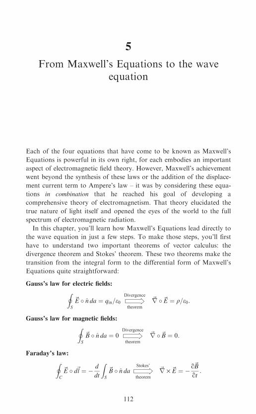
5

From Maxwell’s Equations to the waveequation

Each of the four equations that have come to be known as Maxwell’s

Equations is powerful in its own right, for each embodies an important

aspect of electromagnetic field theory. However, Maxwell’s achievement

went beyond the synthesis of these laws or the addition of the displace-

ment current term to Ampere’s law – it was by considering these equa-

tions in combination that he reached his goal of developing a

comprehensive theory of electromagnetism. That theory elucidated the

true nature of light itself and opened the eyes of the world to the full

spectrum of electromagnetic radiation.

In this chapter, you’ll learn how Maxwell’s Equations lead directly to

the wave equation in just a few steps. To make those steps, you’ll first

have to understand two important theorems of vector calculus: the

divergence theorem and Stokes’ theorem. These two theorems make the

transition from the integral form to the differential form of Maxwell’s

Equations quite straightforward:

Gauss’s law for electric fields:IS

~E � n da ¼ qin=e0Divergence

theorem

~r �~E ¼ q=e0:

Gauss’s law for magnetic fields:IS

~B � n da ¼ 0Divergence

theorem

~r �~B ¼ 0:

Faraday’s law:IC

~E � d~l ¼ � d

dt

ZS

~B � n daStokes’

theorem

~r · ~E ¼ � q~Bqt

:

112

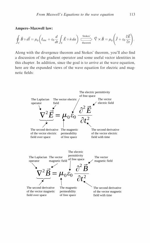
Ampere–Maxwell law:IC


dt

ZS

~E � n da� �

Stokes’

theorem

~r · ~B ¼ l0 ~J þ e0q~Eqt

!:

Along with the divergence theorem and Stokes’ theorem, you’ll also find

a discussion of the gradient operator and some useful vector identities in

this chapter. In addition, since the goal is to arrive at the wave equation,

here are the expanded views of the wave equation for electric and mag-

netic fields:

E� = 0�0��t

E2

22

The Laplacianoperator

The vector electricfield

The electric permittivityof free space

The vectorelectric field

The magneticpermeability of free space

The second derivativeof the vector electricfield over space

The second derivativeof the vector electricfield with time

B� = 0�0��t

B2

22

The Laplacianoperator

The vectormagnetic field


The vectormagnetic field


The second derivativeof the vector magneticfield with time

The second derivativeof the vector magneticfield over space

From Maxwell’s Equations to the wave equation 113

HS~A � n da ¼ R

Vð~r �~AÞ dV The divergence theorem

The divergence theorem is a vector–calculus relation that equates the flux

of a vector field to the volume integral of the field’s divergence. The

relationships between line, surface, and volume integrals were explored by

several of the leading mathematical thinkers of the eighteenth and nine-

teenth centuries, including J. L. LaGrange in Italy, M. V. Ostrogradsky

in Russia, G. Green in England, and C. F. Gauss in Germany. In some

texts, you’ll find the divergence theorem referred to as ‘‘Gauss’s theorem’’

(which you should not confuse with Gauss’s law).

The divergence theorem may be stated as follows:

The flux of a vector field through a closed surface S is equal to the

integral of the divergence of that field over a volume V for which S is

a boundary.

This theorem applies to vector fields that are ‘‘smooth’’ in the sense of

being continuous and having continuous derivatives.

To understand the physical basis for the divergence theorem, recall

that the divergence at any point is defined as the flux through a small

surface surrounding that point divided by the volume enclosed by that

surface as it shrinks to zero. Now consider the flux through the cubical

cells within the volume V shown in Figure 5.1.

For interior cells (those not touching the surface of V), the faces are

shared with six adjacent cells (only some of which are shown in Figure 5.1

for clarity). For each shared face, the positive (outward) flux from one

V

Boundarysurface S

Flux through faces atboundary

Positive flux from an interiorcell is negative flux for anadjacent cell with shared face

Figure 5.1 Cubical cells within volume V bounded by surface S.


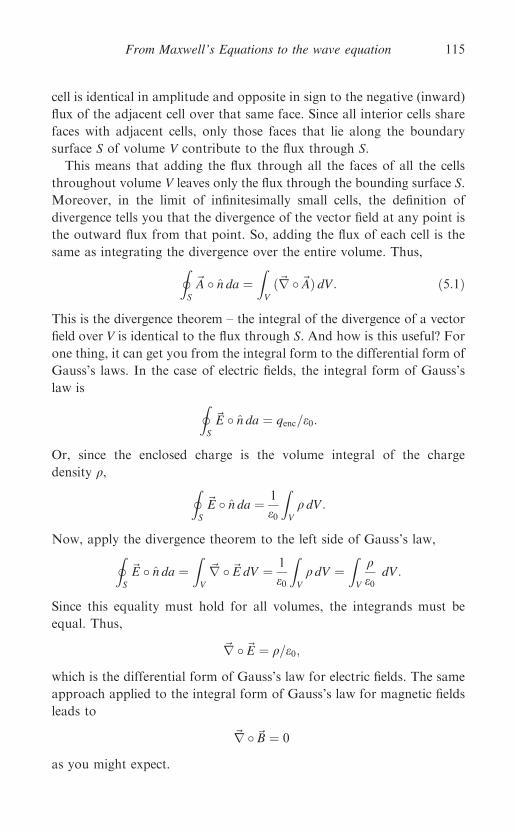
cell is identical in amplitude and opposite in sign to the negative (inward)

flux of the adjacent cell over that same face. Since all interior cells share

faces with adjacent cells, only those faces that lie along the boundary

surface S of volume V contribute to the flux through S.

This means that adding the flux through all the faces of all the cells

throughout volume V leaves only the flux through the bounding surface S.

Moreover, in the limit of infinitesimally small cells, the definition of

divergence tells you that the divergence of the vector field at any point is

the outward flux from that point. So, adding the flux of each cell is the

same as integrating the divergence over the entire volume. Thus,IS

~A � n da ¼ZV

ð~r �~AÞ dV: ð5:1Þ

This is the divergence theorem – the integral of the divergence of a vector

field over V is identical to the flux through S. And how is this useful? For

one thing, it can get you from the integral form to the differential form of

Gauss’s laws. In the case of electric fields, the integral form of Gauss’s

law is IS

~E � n da ¼ qenc=e0:

Or, since the enclosed charge is the volume integral of the charge

density q, IS

~E � n da ¼ 1

e0

ZV

q dV:

Now, apply the divergence theorem to the left side of Gauss’s law,IS

~E � n da ¼ZV

~r �~E dV ¼ 1

e0

ZV

q dV ¼ZV

qe0

dV:

Since this equality must hold for all volumes, the integrands must be

equal. Thus,

~r �~E ¼ q=e0;

which is the differential form of Gauss’s law for electric fields. The same

approach applied to the integral form of Gauss’s law for magnetic fields

leads to

~r �~B ¼ 0

as you might expect.


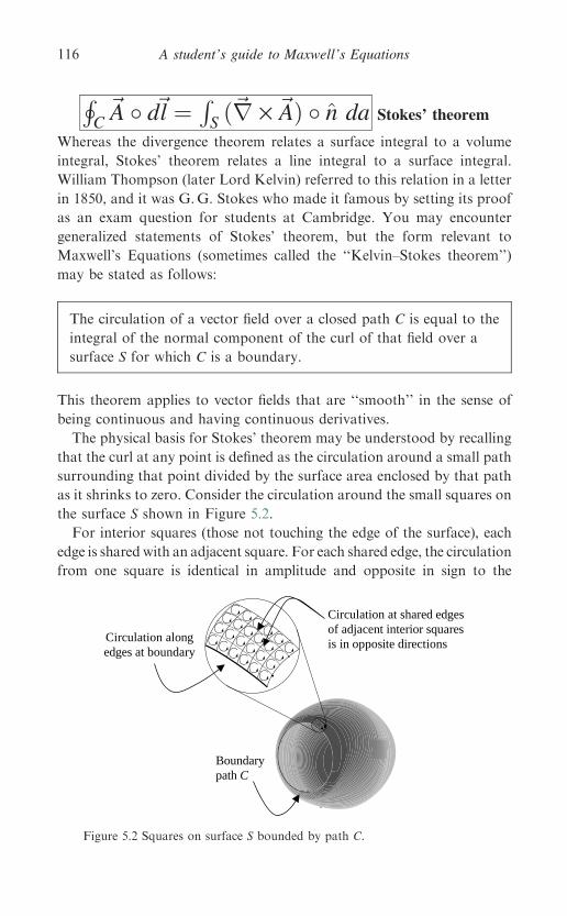
HC~A � d~l ¼ R

Sð~r · ~AÞ � n da Stokes’ theorem

Whereas the divergence theorem relates a surface integral to a volume

integral, Stokes’ theorem relates a line integral to a surface integral.

William Thompson (later Lord Kelvin) referred to this relation in a letter

in 1850, and it was G.G. Stokes who made it famous by setting its proof

as an exam question for students at Cambridge. You may encounter

generalized statements of Stokes’ theorem, but the form relevant to

Maxwell’s Equations (sometimes called the ‘‘Kelvin–Stokes theorem’’)

may be stated as follows:

The circulation of a vector field over a closed path C is equal to the

integral of the normal component of the curl of that field over a

surface S for which C is a boundary.

This theorem applies to vector fields that are ‘‘smooth’’ in the sense of

being continuous and having continuous derivatives.

The physical basis for Stokes’ theorem may be understood by recalling

that the curl at any point is defined as the circulation around a small path

surrounding that point divided by the surface area enclosed by that path

as it shrinks to zero. Consider the circulation around the small squares on

the surface S shown in Figure 5.2.

For interior squares (those not touching the edge of the surface), each

edge is sharedwith an adjacent square. For each shared edge, the circulation

from one square is identical in amplitude and opposite in sign to the

Boundarypath C

Circulation at shared edgesof adjacent interior squaresis in opposite directionsCirculation along

edges at boundary

Figure 5.2 Squares on surface S bounded by path C.


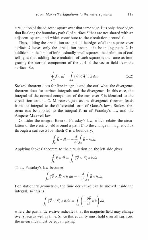
circulation of the adjacent square over that same edge. It is only those edges

that lie along the boundary path C of surface S that are not shared with an

adjacent square, and which contribute to the circulation around C.

Thus, adding the circulation around all the edges of all the squares over

surface S leaves only the circulation around the bounding path C. In

addition, in the limit of infinitesimally small squares, the definition of curl

tells you that adding the circulation of each square is the same as inte-

grating the normal component of the curl of the vector field over the

surface. So, IC

~A � d~l ¼ZS

ð~r · ~AÞ � n da: ð5:2Þ

Stokes’ theorem does for line integrals and the curl what the divergence

theorem does for surface integrals and the divergence. In this case, the

integral of the normal component of the curl over S is identical to the

circulation around C. Moreover, just as the divergence theorem leads

from the integral to the differential form of Gauss’s laws, Stokes’ the-

orem can be applied to the integral form of Faraday’s law and the

Ampere–Maxwell law.

Consider the integral form of Faraday’s law, which relates the circu-

lation of the electric field around a path C to the change in magnetic flux

through a surface S for which C is a boundary,IC

~E � d~l ¼ � d

dt

ZS

~B � n da:

Applying Stokes’ theorem to the circulation on the left side givesIC

~E � d~l ¼ZS

ð~r · ~EÞ � n da

Thus, Faraday’s law becomesZS

ð~r · ~EÞ � n da ¼ � d

dt

ZS

~B � n da:

For stationary geometries, the time derivative can be moved inside the

integral, so this isZS

ð~r · ~EÞ � n da ¼ZS

� @~B

@t� n

!da;

where the partial derivative indicates that the magnetic field may change

over space as well as time. Since this equality must hold over all surfaces,

the integrands must be equal, giving


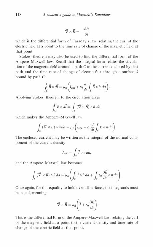
~r · ~E ¼ � @~B

@t;

which is the differential form of Faraday’s law, relating the curl of the

electric field at a point to the time rate of change of the magnetic field at

that point.

Stokes’ theorem may also be used to find the differential form of the

Ampere–Maxwell law. Recall that the integral form relates the circula-

tion of the magnetic field around a path C to the current enclosed by that

path and the time rate of change of electric flux through a surface S

bound by path C:IC


dt

ZS

~E � n da

� �:

Applying Stokes’ theorem to the circulation givesIC

~B � d~l ¼ZS

ð~r · ~BÞ � n da;

which makes the Ampere–Maxwell lawZS

ð~r · ~BÞ � n da ¼ l0 Ienc þ e0d

dt

ZS

~E � n da� �

:

The enclosed current may be written as the integral of the normal com-

ponent of the current density

Ienc ¼ZS

~J � n da;

and the Ampere–Maxwell law becomes

ZS

ð~r · ~BÞ � n da ¼ l0

ZS

~J � n daþZS

e0@~E

@t� n da

!:

Once again, for this equality to hold over all surfaces, the integrands must

be equal, meaning

~r · ~B ¼ l0 ~J þ e0@~E

@t

!:

This is the differential form of the Ampere–Maxwell law, relating the curl

of the magnetic field at a point to the current density and time rate of

change of the electric field at that point.


~rðÞ The gradient

To understand how Maxwell’s Equations lead to the wave equation, it is

necessary to comprehend a third differential operation used in vector

calculus – the gradient. Similar to the divergence and the curl, the gradient

involves partial derivatives taken in three orthogonal directions. However,

whereas the divergence measures the tendency of a vector field to flow

away from a point and the curl indicates the circulation of a vector field

around a point, the gradient applies to scalar fields. Unlike a vector field, a

scalar field is specified entirely by its magnitude at various locations: one

example of a scalar field is the height of terrain above sea level.

What does the gradient tell you about a scalar field? Two important

things: the magnitude of the gradient indicates how quickly the field is

changing over space, and the direction of the gradient indicates the dir-

ection in that the field is changing most quickly with distance.

Therefore, although the gradient operates on a scalar field, the result of

the gradient operation is a vector, with bothmagnitude and direction. Thus,

if the scalar field represents terrain height, the magnitude of the gradient at

any location tells you how steeply the ground is sloped at that location, and

the direction of the gradient points uphill along the steepest slope.

The definition of the gradient of the scalar field w is

gradðwÞ ¼ ~rw � i@w

@xþ j

@w

@yþ k

@w

@zðCartesianÞ: ð5:3Þ

Thus, the x-component of the gradient of w indicates the slope of the

scalar field in the x-direction, the y-component indicates the slope in the

y-direction, and the z-component indicates the slope in the z-direction.

The square root of the sum of the squares of these components provides

the total steepness of the slope at the location at which the gradient is

taken.

In cylindrical and spherical coordinates, the gradient is

~rw � r@w

@rþ ’

1

r

@w

@uþ z

@w

@zðcylindricalÞ ð5:4Þ

and

~rw � r@w@r

þ h1

r

@w@h

þ ’1

r sin h@w@u

ðsphericalÞ: ð5:5Þ


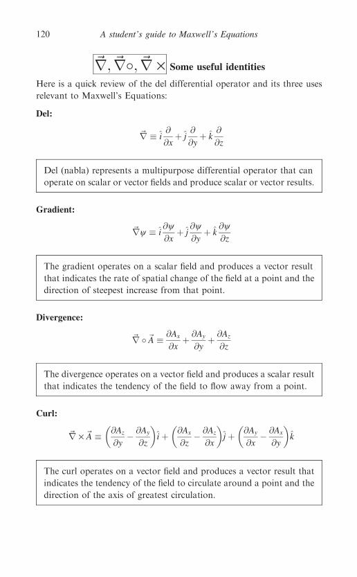
~r; ~r�; ~r · Some useful identities

Here is a quick review of the del differential operator and its three uses

relevant to Maxwell’s Equations:

Del:

~r � i@

@xþ j

@

@yþ k

@

@z

Del (nabla) represents a multipurpose differential operator that can

operate on scalar or vector fields and produce scalar or vector results.

Gradient:

~rw � i@w@x

þ j@w@y

þ k@w@z

The gradient operates on a scalar field and produces a vector result

that indicates the rate of spatial change of the field at a point and the

direction of steepest increase from that point.

Divergence:

~r �~A � @Ax

@xþ @Ay

@yþ @Az

@z

The divergence operates on a vector field and produces a scalar result

that indicates the tendency of the field to flow away from a point.

Curl:

~r · ~A � @Az

@y� @Ay

@z

� �iþ @Ax

@z� @Az

@x

� �jþ @Ay

@x� @Ax

@y

� �k

The curl operates on a vector field and produces a vector result that

indicates the tendency of the field to circulate around a point and the

direction of the axis of greatest circulation.


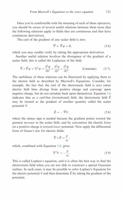
Once you’re comfortable with the meaning of each of these operators,

you should be aware of several useful relations between them (note that

the following relations apply to fields that are continuous and that have

continuous derivatives).

The curl of the gradient of any scalar field is zero.

~r · ~rw ¼ 0; ð5:6Þwhich you may readily verify by taking the appropriate derivatives.

Another useful relation involves the divergence of the gradient of a

scalar field; this is called the Laplacian of the field:

~r � ~rw ¼ r2w ¼ @2w@x2

þ @2w@y2

þ @2w@z2

ðCartesianÞ: ð5:7Þ:

The usefulness of these relations can be illustrated by applying them to

the electric field as described by Maxwell’s Equations. Consider, for

example, the fact that the curl of the electrostatic field is zero (since

electric field lines diverge from positive charge and converge upon

negative charge, but do not circulate back upon themselves). Equation 5.6

indicates that as a curl-free (irrotational) field, the electrostatic field ~E

may be treated as the gradient of another quantity called the scalar

potential V:

~E ¼ � ~rV ; ð5:8Þwhere the minus sign is needed because the gradient points toward the

greatest increase in the scalar field, and by convention the electric force

on a positive charge is toward lower potential. Now apply the differential

form of Gauss’s law for electric fields:

~r �~E ¼ qe0;

which, combined with Equation 5.8, gives

r2V ¼ � qe0: ð5:9Þ

This is called Laplace’s equation, and it is often the best way to find the

electrostatic field when you are not able to construct a special Gaussian

surface. In such cases, it may be possible to solve Laplace’s Equation for

the electric potential V and then determine ~E by taking the gradient of the

potential.


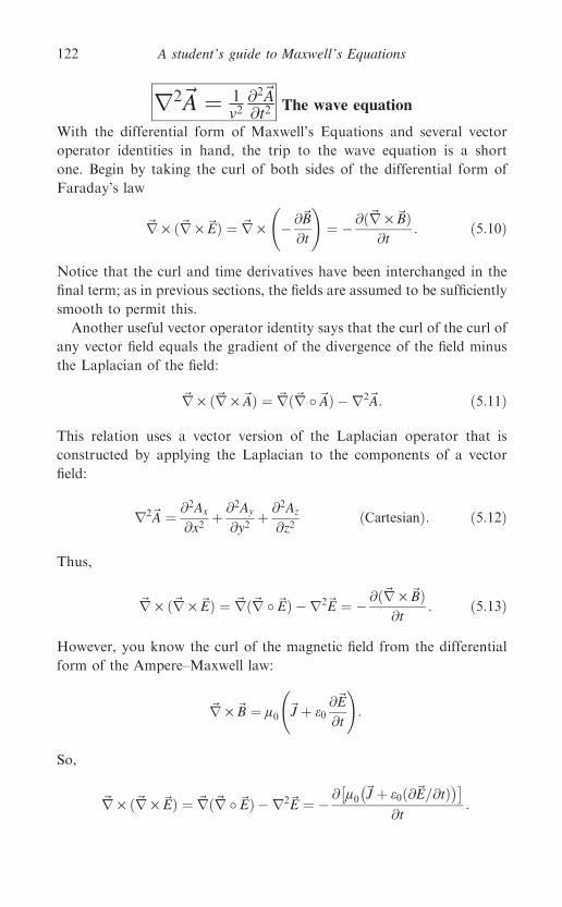
r2~A ¼ 1v2

@2~A@t2

The wave equation

With the differential form of Maxwell’s Equations and several vector

operator identities in hand, the trip to the wave equation is a short

one. Begin by taking the curl of both sides of the differential form of

Faraday’s law

~r · ð~r · ~EÞ ¼ ~r · � @~B

@t

!¼ � @ð~r · ~BÞ

@t: ð5:10Þ

Notice that the curl and time derivatives have been interchanged in the

final term; as in previous sections, the fields are assumed to be sufficiently

smooth to permit this.

Another useful vector operator identity says that the curl of the curl of

any vector field equals the gradient of the divergence of the field minus

the Laplacian of the field:

~r · ð~r · ~AÞ ¼ ~rð~r �~AÞ � r2~A: ð5:11Þ

This relation uses a vector version of the Laplacian operator that is

constructed by applying the Laplacian to the components of a vector

field:

r2~A ¼ @2Ax

@x2þ @2Ay

@y2þ @2Az

@z2ðCartesianÞ: ð5:12Þ

Thus,

~r · ð~r · ~EÞ ¼ ~rð~r �~EÞ � r2~E ¼ � @ð~r · ~BÞ@t

: ð5:13Þ

However, you know the curl of the magnetic field from the differential

form of the Ampere–Maxwell law:

~r · ~B ¼ l0 ~J þ e0@~E

@t

!:

So,

~r · ð~r · ~EÞ ¼ ~rð~r �~EÞ � r2~E ¼ � @ l0 ~J þ e0ð@~E=@tÞ� ��

@t:


This looks difficult, but one simplification can be achieved using Gauss’s

law for electric fields:

~r �~E ¼ qe0;

which means

~r · ð~r · ~EÞ ¼ ~r qe0

� ��r2~E ¼ � @ l0 ~J þ e0ð@~E=@tÞ

� �� @t

¼ �l0@~J

@t� l0e0

@2~E

@t2:

Gathering terms containing the electric field on the left side of this

equation gives

r2~E � l0e0@2~E

@t2¼ ~r q

e0

� �þ l0

@~J

@t:

In a charge- and current-free region, q = 0 and ~J ¼ 0, so

r2~E ¼ l0e0@2~E

@t2: ð5:14Þ

This is a linear, second-order, homogeneous partial differential equation

that describes an electric field that travels from one location to another –

in short, a propagating wave. Here is a quick reminder of the meaning of

each of the characteristics of the wave equation:

Linear: The time and space derivatives of the wave function (~E in this

case) appear to the first power and without cross terms.

Second-order: The highest derivative present is the second derivative.

Homogeneous: All terms involve the wave function or its derivatives, so

no forcing or source terms are present.

Partial: The wave function is a function of multiple variables (space and

time in this case).

A similar analysis beginning with the curl of both sides of the Ampere–

Maxwell law leads to

r2~B ¼ l0e0@2~B

@t2; ð5:15Þ

which is identical in form to the wave equation for the electric field.

This form of the wave equation doesn’t just tell you that you have a

wave – it provides the velocity of propagation as well. It is right there in


the constants multiplying the time derivative, because the general form of

the wave equation is this

r2~A ¼ 1

v2@2~A

@t2; ð5:16Þ

where v is the speed of propagation of the wave. Thus, for the electric and

magnetic fields

1

v2¼ l0e0;

or

v ¼ffiffiffiffiffiffiffiffiffi1

l0e0

s: ð5:17Þ

Inserting values for the magnetic permeability and electric permittivity of

free space,

v ¼ffiffiffiffiffiffiffiffiffiffiffiffiffiffiffiffiffiffiffiffiffiffiffiffiffiffiffiffiffiffiffiffiffiffiffiffiffiffiffiffiffiffiffiffiffiffiffiffiffiffiffiffiffiffiffiffiffiffiffiffiffiffiffiffiffiffiffiffiffiffiffiffiffiffiffiffiffiffiffiffiffiffiffiffiffiffiffiffiffiffiffiffiffiffiffiffiffiffiffiffiffiffiffiffiffiffiffi

1

½4p · 10�7m kg=C2�½8:8541878 · 10�12 C2 s2=kg m3� ;s

or

v ¼ffiffiffiffiffiffiffiffiffiffiffiffiffiffiffiffiffiffiffiffiffiffiffiffiffiffiffiffiffiffiffiffiffiffiffiffiffiffiffiffiffiffiffi8:987552·1016 m2=s2

q¼ 2:9979 · 108 m=s:

It was the agreement of the calculated velocity of propagation with the

measured speed of light that caused Maxwell to write, ‘‘light is an elec-

tromagnetic disturbance propagated through the field according to

electromagnetic laws.’’


Appendix: Maxwell’s Equationsin matter

Maxwell’s Equations as presented in Chapters 1–4 apply to electric and

magnetic fields in matter as well as in free space. However, when you’re

dealing with fields inside matter, remember the following points:

� The enclosed charge in the integral form of Gauss’s law for electric

fields (and current density in the differential form) includes ALL

charge – bound as well as free.

� The enclosed current in the integral form of the Ampere–Maxwell law

(and volume current density in the differential form) includes ALL

currents – bound and polarization as well as free.

Since the bound charge may be difficult to determine, in this Appendix

you’ll find versions of the differential and integral forms of Gauss’s law

for electric fields that depend only on the free charge. Likewise, you’ll find

versions of the differential and integral form of the Ampere–Maxwell law

that depend only on the free current.

What about Gauss’s law for magnetic fields and Faraday’s law? Since

those laws don’t directly involve electric charge or current, there’s no

need to derive more “matter friendly” versions of them.

Gauss’s law for electric fields: Within a dielectric material, positive and

negative charges may become slightly displaced when an electric field is

applied. When a positive charge Q is separated by distance s from an

equal negative charge −Q, the electric “dipole moment” is given by

~p ¼ Q~s; ðA:1Þ

where~s is a vector directed from the negative to the positive charge with

magnitude equal to the distance between the charges. For a dielectric

125

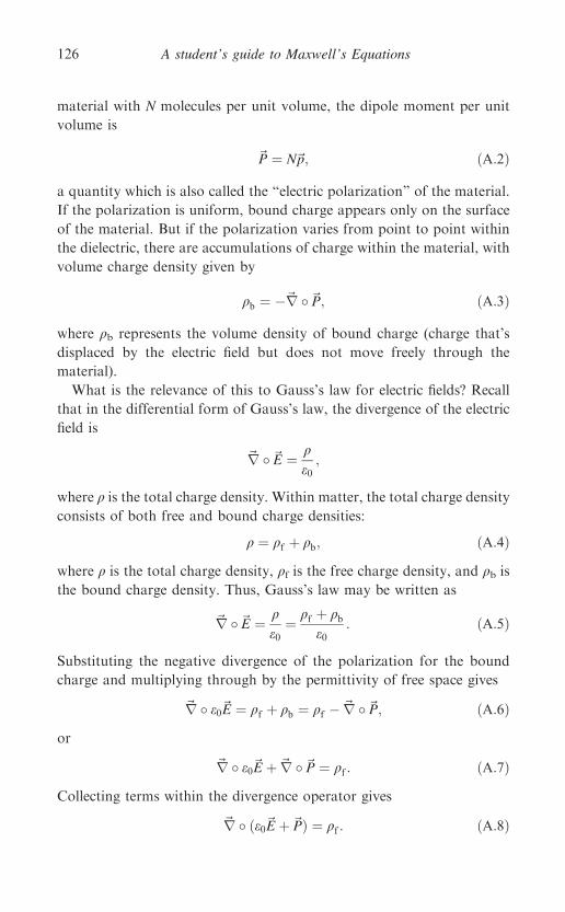
material with N molecules per unit volume, the dipole moment per unit

volume is

~P ¼ N~p; ðA:2Þ

a quantity which is also called the “electric polarization” of the material.

If the polarization is uniform, bound charge appears only on the surface

of the material. But if the polarization varies from point to point within

the dielectric, there are accumulations of charge within the material, with

volume charge density given by

qb ¼ �~r �~P; ðA:3Þ

where qb represents the volume density of bound charge (charge that’s

displaced by the electric field but does not move freely through the

material).

What is the relevance of this to Gauss’s law for electric fields? Recall

that in the differential form of Gauss’s law, the divergence of the electric

field is

~r �~E ¼ qe0;

where q is the total charge density. Within matter, the total charge density

consists of both free and bound charge densities:

q ¼ qf þ qb; ðA:4Þwhere q is the total charge density, qf is the free charge density, and qb isthe bound charge density. Thus, Gauss’s law may be written as

~r �~E ¼ qe0

¼ qf þ qbe0

: ðA:5Þ

Substituting the negative divergence of the polarization for the bound

charge and multiplying through by the permittivity of free space gives

~r � e0~E ¼ qf þ qb ¼ qf � ~r �~P; ðA:6Þor

~r � e0~E þ ~r �~P ¼ qf : ðA:7ÞCollecting terms within the divergence operator gives

~r � ðe0~E þ~PÞ ¼ qf : ðA:8Þ


In this form of Gauss’s law, the term in parentheses is often written as a

vector called the “displacement,” which is defined as

~D ¼ e0~E þ~P: ðA:9ÞSubstituting this expression into equation (A.8) gives

~r � ~D ¼ qf ; ðA:10Þwhich is a version of the differential form of Gauss’s law that depends

only on the density of free charge.

Using the divergence theorem gives the integral form of Gauss’s law

for electric fields in terms of the flux of the displacement and enclosed free

charge: IS

~D � n da ¼ qfree; enc: ðA:11Þ

What is the physical significance of the displacement ~D? In free space, the

displacement is a vector field proportional to the electric field – pointing in

the same direction as ~E and with magnitude scaled by the vacuum permit-

tivity. But in polarizable matter, the displacement field may differ signifi-

cantly from the electric field. You should note, for example, that the

displacement is not necessarily irrotational – it will have curl if the polar-

ization does, as can be seen by taking the curl of both sides of Equation A.9.

The usefulness of ~D comes about in situations for which the free charge

is known and for which symmetry considerations allow you to extract the

displacement from the integral of Equation A.11. In those cases, you may

be able to determine the electric field within a linear dielectric material

by finding ~D on the basis of the free charge and then dividing by the

permittivity of the medium to find the electric field.

The Ampere–Maxwell law: Just as applied electric fields induce polar-

ization (electric dipole moment per unit volume) within dielectrics, applied

magnetic fields induce “magnetization” (magnetic dipole moment per unit

volume) within magnetic materials. And just as bound electric charges act

as the source of additional electric fields within the material, bound cur-

rents may act as the source of additional magnetic fields. In that case, the

bound current density is given by the curl of the magnetization:

~Jb ¼ ~r · ~M: ðA:12Þwhere~Jb is the bound current density and ~M represents the magnetization

of the material.

Appendix 127

Another contribution to the current density within matter comes

from the time rate of change of the polarization, since any movement of

charge constitutes an electric current. The polarization current density is

given by

~JP ¼ @~P

@t: ðA:13Þ

Thus, the total current density includes not only the free current density,

but the bound and polarization current densities as well:

~J ¼~Jf þ~Jb þ~JP: ðA:14Þ

Thus, the Ampere–Maxwell law in differential form may be written as

~r · ~B ¼ l0 ~Jf þ ~Jb þ ~JP þ e0@~E

@t

!: ðA:15Þ

Inserting the expressions for the bound and polarization current and

dividing by the permeability of free space

1

l0~r · ~B ¼ ~Jf þ ~r · ~M þ @~P

@tþ e0

@~E

@t: ðA:16Þ

Gathering curl terms and time-derivative terms gives

~r ·~B

l0� ~r · ~M ¼ ~Jf þ @~P

@tþ @ðe0~EÞ

@t: ðA:17Þ

Moving the terms inside the curl and derivative operators makes this

~r ·~B

l0� ~M

!¼ ~Jf þ @ðe0~E þ~PÞ

@t: ðA:18Þ

In this form of the Ampere–Maxwell law, the term in parentheses on the

left side is written as a vector sometimes called the “magnetic field

intensity” or “magnetic field strength” and defined as

~H ¼~B

l0� ~M: ðA:19Þ

Thus, the differential form of the Ampere–Maxwell law in terms of ~H, ~D,

and the free current density is


~r · ~H ¼~Jfree þ @~D

@t: ðA:20Þ

Using Stokes’ theorem gives the integral form of the Ampere–Maxwell

law: IC

~H � ~dl ¼ Ifree; enc þ d

dt

ZS

~D � n da ðA:21Þ

What is the physical significance of the magnetic intensity ~H? In free

space, the intensity is a vector field proportional to the magnetic field –

pointing in the same direction as ~B and with magnitude scaled by the

vacuum permeability. But just as ~D may differ from ~E inside dielectric

materials, ~H may differ significantly from ~B in magnetic matter. For

example, the magnetic intensity is not necessarily solenoidal – it will have

divergence if the magnetization does, as can be seen by taking the

divergence of both sides of Equation A.19.

As is the case for electric displacement, the usefulness of ~H comes

about in situations for which you know the free current and for which

symmetry considerations allow you to extract the magnetic intensity from

the integral of Equation A.21. In such cases, you may be able to deter-

mine the magnetic field within a linear magnetic material by finding ~H on

the basis of free current and then multiplying by the permeability of the

medium to find the magnetic field.

Appendix 129

Here is a summary of the integral and differential forms of all of

Maxwell’s Equations in matter:

Gauss’s law for electric fields:IS

~D � n da ¼ qfree; enc ðintegral formÞ;

~r � ~D ¼ qfree ðdifferential formÞ:

Gauss’s law for magnetic fields:IS

~B � n da ¼ 0 ðintegral formÞ;

~r �~B ¼ 0 ðdifferential formÞ:

Faraday’s law:IC

~E � d~l ¼ � d

dt

ZS

~B � n da ðintegral formÞ;

~r · ~E ¼ � @~B

@tðdifferential formÞ:

Ampere–Maxwell law:IC

~H � d~l ¼ Ifree; enc þ d

dt

ZS

~D � n da ðintegral formÞ;

~r · ~H ¼~Jfree þ @~D

@tðdifferential formÞ:


Further reading

If you’re looking for a comprehensive treatment of electricity and magnetism, youhave several excellent texts from which to choose. Here are some that you may

find useful:

Cottingham W. N. and Greenwood D. A., Electricity and Magnetism. CambridgeUniversity Press, 1991; A concise survey of a wide range of topics in

electricity and magnetism.Griffiths, D. J., Introduction to Electrodynamics. Prentice-Hall, New Jersey, 1989;

The standard undergraduate text at the intermediate level, with clear

explanations and informal style.Jackson, J. D., Classical Electrodynamics. Wiley & Sons, New York, 1998; The

standard graduate text, but you must be solidly prepared before embarking.Lorrain, P., Corson, D., and Lorrain, F., Electromagnetic Fields and Waves.

Freeman, New York, 1988; Another excellent intermediate-level text, withdetailed explanations supported by helpful diagrams.

Purcell, E. M., Electricity and Magnetism Berkeley Physics Course, Vol. 2.

McGraw-Hill, New York, 1965; Probably the best of the introductory-leveltexts; elegantly written and carefully illustrated.

Wangsness, R. K., Electromagnetic Fields. Wiley, New York, 1986; Also a great

intermediate-level text, especially useful as preparation for Jackson.And for a comprehensible introduction to vector operators, with many examples

drawn from electrostatics, check out:

Schey, H. M., Div, Grad, Curl, and All That. Norton, New York, 1997.

131

Index

Ampere, Andre-Marie 83Ampere-- Maxwell law 83 -- 111

differential form 101--9applying 108--9expanded view 101main idea 101version involving only free

current 128integral form 83--100applying 95--100expanded view 84main idea 84usefulness of 84version involving only free

current 129Ampere’s law 83

Biot-- Savart law 47

capacitance 18--19of a parallel-plate capacitor 18

charge, electricbound 18, 126density 16enclosed 16--17relationship to flux 17

circulation 65of electric field 68of magnetic field 85--6

closed surface 7curl 76--8

in Cartesian coordinates 77of electric field 79locating regions of 76--7of magnetic field 102--4main idea 120in non-Cartesian coordinates 78relationship to circulation 76

current density 105--6bound 127

polarization 128units of 105

del cross (see curl)del dot (see divergence)del operator (see nabla)dielectric constant 19dielectrics 18--19dipole moment, electric 125displacement 127physical significance of 127usefulness of 127

displacement current 94units of 107

divergence 32--5in Cartesian coordinates 33locating regions of 32main idea 120in non-Cartesian coordinates 35relationship to flux 32

divergence theorem 114--15main idea 114

dot product 6how to compute 6physical significance 6

electric fielddefinition of 3electrostatic vs. induced 1, 62--3equations for simple objects 5induced 62--3

direction of 63units of 3, 62

electromotive force (emf) 68units of 68

enclosed current 89--90

Faraday, Michaeldemonstration of induction 58refers to ‘‘field of force’’ 3

132

Faraday’s law 58--82differential form 75--81

applying 79--81expanded view 75main idea 75

integral form 58--74applying 72--4expanded view 60main idea 59usefulness of 61

field lines 3, 13--14fluxelectric 13--15

rate of change of 91--4units of 13

magnetic 48--9rate of change of 69--70units of (see webers)

as number of field lines 13--14of a vector field 10--12

Gauss, C. F. 114Gauss’s law for electric fields 1--41differential form 29--40

applying 38--40expanded view 30main idea 29usefulness of 30version involving only free

charge 127integral form 1--28

applying 20--8expanded view 2main idea 1usefulness of 2version involving only free charge 127

Gauss’s law for magnetic fields 43--57differential form 53--6

applying 55--6expanded view 53main idea 53

integral form 43--52applying 50--2expanded view 44main idea 44usefulness of 44

Gauss’s theorem 114gradient 119--20in Cartesian coordinates 119in non-Cartesian coordinates 119main idea 120

Green, G. 114

Heaviside, Oliver 32

induced current 68direction of 71

inductance 88insulators (see dielectrics)irrotational fields 78

Kelvin-- Stokes theorem 116

LaGrange, J. L. 114Laplacian operator 121

vector version 122Laplace’s equation 121Lenz, Heinrich 71Lenz’s law 71line integral 64Lorentz equation 45

magnetic fielddefinition of 45distinctions from electric field 45equations for simple objects 47intensity 128

physical significance of 129usefulness of 129

units of 45magnetic flux density 45magnetic induction 45magnetic poles 43

always in pairs 44magnetization 127Maxwell, James Clerk

coining of ‘‘convergence’’ 32coining of ‘‘curl’’ 76definition of electric field 3electromagnetic theory 112use of magnetic vortex model 91

nabla 31main idea 120

Oersted, Hans Christian 83Ohm’s law 73open surface 7Ostrogradsky, M.V. 114

path integral 65--7permeability

of free space 87--8relative 87--8

permittivityof free space 18--19relative 19

polarization, electric 126relationship to bound charge 126

scalar field 119scalar potential 121scalar product (see dot product)solenoidal fields 54special Amperian loop 86, 95--100

Index 133

special Gaussian surface 25speed of light 124Stokes, G.G. 116Stokes’ theorem 116--19

main idea 116surface integral 9

Thompson, William 116

unit normal vector 7direction of 7

vacuum permittivity (see permittivityof free space)

vector cross product 45vector field 10

wave equation 122--4for electric fields 113for magnetic fields 113

webers 48work done along a path 65--6

Index134

maxwell's equations - ecuaciones de maxwell libro

Engineering

iax jay kaz

x2 y2 z2

xb0 sinkz

cambridge

highly symmetric

electromagnetic

l0 4p id

circulating