lecture notes on discrete-time finance parts in the lecture notes were based on the materials in...
TRANSCRIPT

Lecture Notes on Discrete-time Finance
Chuanshu Ji
Fall 1998

Most parts in the lecture notes were based on the materials in Pliska’s excellent bookIntroduction to Mathematical Finance (1997, Blackwell Publishers Inc.) except for theBlack-Scholes option pricing formula, and the implied volatility trees.
The required mathematical background is minimal: calculus, linear algebra, calculus-based probability and statistics. Some knowledge of elementary optimization and financialengineering would certainly be useful, but not crucial. In particular, no knowledge ofstochastic calculus is needed. Instead, the focus will be on discrete-time models, such asbinomial trees. We plan to take the approach to as far as we can go, including the treatmentfor stock and fixed-income derivatives. This approach might lose the beauty or even thesimplicity of certain formulas derived via stochastic calculus. Nevertheless, it enables us to
(a) present almost all useful results by using only elementary mathematics;
(b) build up our intuition more quickly;
(c) learn some numerical computation methods directly.
We will attempt at introducing the related continuous-time limit in the late stage of eachchapter, yet we only do so via some basic calculation without invoking weak convergenceof stochastic processes, i.e. we are limited to verify the convergence in finite-dimensionaldistributions, but not the “tightness”.
i
TABLE OF CONTENTS
1 Model Specifications 1
1.1 Asset price dynamics . . . . . . . . . . . . . . . . . . . . . . . . . . . . . . . 1
1.2 Trading strategies . . . . . . . . . . . . . . . . . . . . . . . . . . . . . . . . 2
1.3 Value processes, gain processes and self-financing strategies . . . . . . . . . 2
1.4 Discounted prices . . . . . . . . . . . . . . . . . . . . . . . . . . . . . . . . . 3
2 Binomial Trees: an Example 5
2.1 Illustration of concepts introduced in Lecture 1 . . . . . . . . . . . . . . . . 5
2.2 What is a fair price? . . . . . . . . . . . . . . . . . . . . . . . . . . . . . . . 8
2.3 Risk neutral probabilities . . . . . . . . . . . . . . . . . . . . . . . . . . . . 12
3 Arbitrage and Risk Neutral Probability Measures 13
3.1 Some economic considerations . . . . . . . . . . . . . . . . . . . . . . . . . . 13
3.2 Proof of Theorem 3.1: sufficiency “⇐=” . . . . . . . . . . . . . . . . . . . . 14
3.3 Proof of Theorem 3.1: necessity “=⇒” . . . . . . . . . . . . . . . . . . . . . 15
4 Risk Neutral Valuation of Contingent Claims 17
4.1 Law of one price and risk neutral valuation principle . . . . . . . . . . . . . 17
4.2 Complete markets . . . . . . . . . . . . . . . . . . . . . . . . . . . . . . . . 18
5 Binomial Trees: a General Setting 20
5.1 The basic binomial tree model . . . . . . . . . . . . . . . . . . . . . . . . . 20
5.2 Option pricing using binomial trees . . . . . . . . . . . . . . . . . . . . . . . 21
ii

6 The Black-Scholes Option Pricing Formula 23
7 American Options as Optimal Stopping Problems 26
7.1 A special case: “American = European” . . . . . . . . . . . . . . . . . . . . 26
7.2 Optimal stopping . . . . . . . . . . . . . . . . . . . . . . . . . . . . . . . . . 27
8 More on Valuation of American Options 32
8.1 “American calls = European calls” . . . . . . . . . . . . . . . . . . . . . . . 32
8.2 Options on a dividend-paying stock . . . . . . . . . . . . . . . . . . . . . . . 33
9 Return and Risk 35
9.1 Return processes . . . . . . . . . . . . . . . . . . . . . . . . . . . . . . . . . 35
9.2 Risk premium (single period) . . . . . . . . . . . . . . . . . . . . . . . . . . 36
10 Optimal Portfolios 39
10.1 Optimal portfolios . . . . . . . . . . . . . . . . . . . . . . . . . . . . . . . . 39
10.2 Computation via dynamic programming . . . . . . . . . . . . . . . . . . . . 40
11 Optimization via EMMs 42
11.1 Basic approach . . . . . . . . . . . . . . . . . . . . . . . . . . . . . . . . . . 42
11.2 Examples . . . . . . . . . . . . . . . . . . . . . . . . . . . . . . . . . . . . . 43
12 The Binomial Capital Asset Pricing Model 45
13 Cash Flows and Forward Prices 48
13.1 Dividends and returns . . . . . . . . . . . . . . . . . . . . . . . . . . . . . . 48
13.2 Forward contracts and prices . . . . . . . . . . . . . . . . . . . . . . . . . . 49
14 Futures Contracts 53
14.1 Futures vs forward contracts . . . . . . . . . . . . . . . . . . . . . . . . . . 53
14.2 Futures prices . . . . . . . . . . . . . . . . . . . . . . . . . . . . . . . . . . . 54
14.3 Options on futures . . . . . . . . . . . . . . . . . . . . . . . . . . . . . . . . 57
iii

15 Zero-coupon Bonds, Yields and Forward Rates 59
16 Examples of Term Structure Models 62
17 Spot Rate Modelling via Markov Chains and Stochastic Difference Equa-tions 68
17.1 Spot rate Markov chains . . . . . . . . . . . . . . . . . . . . . . . . . . . . . 68
17.2 Stochastic difference equations . . . . . . . . . . . . . . . . . . . . . . . . . 70
18 Vasicek, Cox-Ingersoll-Ross, and Hull-White Models 72
18.1 Vasicek and CIR models . . . . . . . . . . . . . . . . . . . . . . . . . . . . . 72
18.2 Hull-White model . . . . . . . . . . . . . . . . . . . . . . . . . . . . . . . . . 73
18.3 Refined lattice and SDE . . . . . . . . . . . . . . . . . . . . . . . . . . . . . 73
19 Heath-Jarrow-Morton Approach and Ho-Lee Model 75
19.1 HJM setting . . . . . . . . . . . . . . . . . . . . . . . . . . . . . . . . . . . . 75
19.2 Ho-Lee model . . . . . . . . . . . . . . . . . . . . . . . . . . . . . . . . . . . 77
19.3 Spot rate models from Ho-Lee . . . . . . . . . . . . . . . . . . . . . . . . . . 79
20 Forward Risk Adjusted Probability Measures 80
21 Bond Options and Coupon Bonds 83
22 Swaps, Caps and Floors 86
22.1 Swaps and swaptions . . . . . . . . . . . . . . . . . . . . . . . . . . . . . . . 86
22.2 Caps and floors . . . . . . . . . . . . . . . . . . . . . . . . . . . . . . . . . . 88
23 Implied Volatility 90
23.1 Inverting the Black-Scholes formula . . . . . . . . . . . . . . . . . . . . . . . 90
23.2 Volatility smile . . . . . . . . . . . . . . . . . . . . . . . . . . . . . . . . . . 92
24 Implied Volatility Trees 94
24.1 Construction of implied volatility trees via forward induction . . . . . . . . 94
iv

24.2 Specification of Vput via Arrow-Debreu securities . . . . . . . . . . . . . . . 96
24.3 How to deal with possible bad probabilities? . . . . . . . . . . . . . . . . . . 97
v

Chapter 1
Model Specifications
1.1 Asset price dynamics
To model the financial market statistically, several basic elements are needed.
• A finite sample space Ω = ω1, . . . , ωK.
• A probability measure P on Ω with P (ω) > 0 ∀ ω ∈ Ω.
• A filtration FF = Ft, t = 0, 1, . . . , T with Ft−1 ⊆ Ft, t = 1, . . . , T , where Ft contains theinformation about the financial market available to the investors at time t. Usually,t = 0, 1, . . . , T represent T + 1 trading dates. Since T < ∞, this is called a finitehorizon model or a multiperiod model.
• A riskless bank account process B = B(t), t = 0, 1, . . . , T, where B(0) = 1 andB(t) > 0 ∀t. B(t) is thought of as the time t value of a saving account when $1is deposited at time 0. Hence B(t) is nondecreasing in t. Moreover, the quantityr(t) = [B(t) − B(t − 1)]/B(t − 1) is thought of as the interest rate pertaining to thetime interval (t− 1, t].
• N risky security processes Sn = Sn(t), t = 0, 1, . . . , T, n = 1, . . . , N , where Sn(t) ≥ 0is thought of as the time t price of risky security n (e.g. stock or bond).
Note that B, S1, . . . , SN are considered to be stochastic processes, i.e. for each t, B(t),S1(t), . . . , SN (t) are all functions of ω. To ease the notation, the dependence on ω is usuallynot shown unless necessary. Furthermore, B, S1, . . . , SN are assumed to be adapted to thefiltration FF . A stochastic process X(t) is said to be adapted to the filtration FF if foreach t, the random variable X(t) is measurable with respect to Ft, i.e. the informationabout X(t) is contained in Ft.
1

1.2 Trading strategies
A trading strategy h = (h0, h1, . . . , hN ) is a vector of processes hn = hn(t), t = 1, . . . , T,n = 0, 1, . . . , N . Note that hn(0) is not specified, because for n = 1, . . . , N , hn(t) isinterpreted as the number of units (e.g. shares of stock) that the investor owns (i.e. carriesforward) from time t− 1 to time t, whereas h0(t) B(t− 1) represents the amount of moneyinvested in the bank account at time t − 1. A negative value of hn(t) corresponds toborrowing money from the bank (when n = 0) or selling short security n (when n =1, . . . , N). h is also called a portfolio.
A trading strategy is a rule that specifies the investor’s position in each security n ateach time t and in each state of the world ω. In general, this rule should allow the investorto choose a position in the securities based on the available information thus far without“looking into the future”. This is done by introducing the concept of predictability.
A stochastic process X(t) is said to be predictable with respect to the filtration FF iffor each t = 1, 2, . . . the random variable X(t) is measurable with respect to Ft−1. (Note:“predictable” implies “adapted”, why?) In what follows we assume that each componentof a trading strategy h is a predictable process.
1.3 Value processes, gain processes and self-financing strate-
gies
The value process V = V (t), t = 0, 1, . . . , T consists of the initial value of the portfolio
V (0) = h0(1)B(0) +N∑
n=1
hn(1)Sn(0) (1.1)
and the time t (t ≥ 1) value of the portfolio
V (t) = h0(t)B(t) +N∑
n=1
hn(t)Sn(t) (1.2)
before any transactions are made at the same time. (Note: V is adapted, why?)
Denote ∆Sn(t) = Sn(t)− Sn(t− 1) for the increment of Sn between t− 1 and t. Thenhn(t) ∆Sn(t) represents the one-period gain or loss due to the ownership of hn(t) units ofsecurity n between t− 1 and t; and
∑tu=1 hn(u) ∆Sn(u) represents the cumulative gain or
loss up to time t due to the investment of security n. Hence
G(t) =t∑
u=1
h0(u) ∆B(u) +N∑
n=1
t∑
u=1
hn(u) ∆Sn(u) (1.3)
2

represents the cumulative gain or loss of the portfolio up to time t. G = G(t), t = 1, . . . , Tis called a gain process (also adapted, why?).
A trading strategy is said to be self-financing if for t = 1, . . . , T − 1,
V (t) = h0(t + 1) B(t) +N∑
n=1
hn(t + 1) Sn(t). (1.4)
The motivation is that the LHS represents the time t value of the portfolio just before anytransactions (i.e. any changes of ownership positions) take place at that time, while theRHS represents the time t value of the portfolio right after any transactions (i.e. beforethe portfolio is carried forward to t + 1). In general, the two values can be different, whichmeans at time t some money is added to or withdrawn from the portfolio. However, formany applications this cannot happen at other than t = 0 and t = T , and so it leads to theabove definition. For a self-financing strategy, any change in the portfolio’s value is due toa gain or loss in the investments.
It is straightforward to check (do it yourself) the following: A strategy h is self-financingif and only if
V (t) = V (0) + G(t), t = 1, . . . , T. (1.5)
Note that V (1) = V (0) + G(1) always holds (why?).
1.4 Discounted prices
For the studies of finance modelling, what really matters is the behavior of the securityprices relative to each other, rather than their absolute behavior. Hence we are interestedin normalized versions of the security prices with respect to the price of a standard security— usually using the bank account for convenience. In general, some other riskless securitiescould be chosen as the “yardstick”, called the numeraire.
Define the discounted price processes S∗n = S∗n(t), t = 0, 1, . . . , T, n = 1, . . . , N by
S∗n(t) = Sn(t)/B(t), t = 0, 1, . . . , T ; (1.6)
the discounted value process V ∗ = V ∗(t), t = 0, 1, . . . , T by
V ∗(0) = h0(1) +N∑
n=1
hn(1)S∗n(0) (1.7)
and
V ∗(t) = h0(t) +N∑
n=1
hn(t)S∗n(t); (1.8)
3

and the discounted gain process G∗ = G∗(t), t = 1, . . . , T by
G∗(t) =N∑
n=1
t∑
u=1
hn(u) ∆S∗n(u), t = 1, . . . , T. (1.9)
Note in particular, B∗(t) = 1 and ∆B∗(t) = 0, ∀t. It is also easy to check:
V ∗(t) = V (t)/B(t), t = 0, 1, . . . , T ; (1.10)
and that a strategy h is self-financing if and only if
V ∗(t) = V ∗(0) + G∗(t), t = 1, . . . , T. (1.11)
4
Chapter 2
Binomial Trees: an Example
2.1 Illustration of concepts introduced in Lecture 1
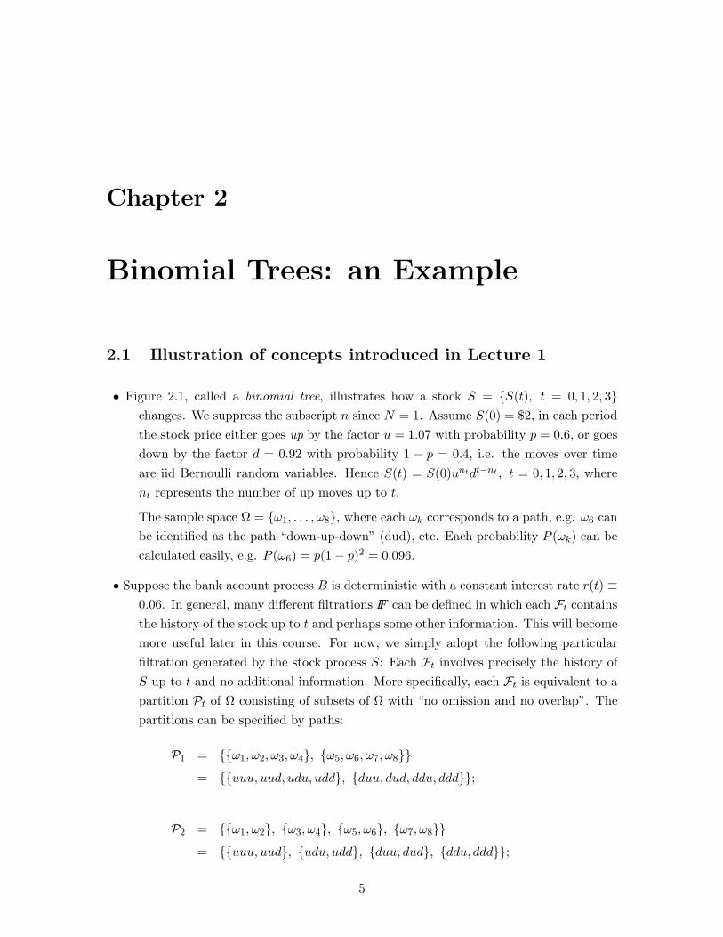
• Figure 2.1, called a binomial tree, illustrates how a stock S = S(t), t = 0, 1, 2, 3changes. We suppress the subscript n since N = 1. Assume S(0) = $2, in each periodthe stock price either goes up by the factor u = 1.07 with probability p = 0.6, or goesdown by the factor d = 0.92 with probability 1 − p = 0.4, i.e. the moves over timeare iid Bernoulli random variables. Hence S(t) = S(0)untdt−nt , t = 0, 1, 2, 3, wherent represents the number of up moves up to t.
The sample space Ω = ω1, . . . , ω8, where each ωk corresponds to a path, e.g. ω6 canbe identified as the path “down-up-down” (dud), etc. Each probability P (ωk) can becalculated easily, e.g. P (ω6) = p(1− p)2 = 0.096.
• Suppose the bank account process B is deterministic with a constant interest rate r(t) ≡0.06. In general, many different filtrations FF can be defined in which each Ft containsthe history of the stock up to t and perhaps some other information. This will becomemore useful later in this course. For now, we simply adopt the following particularfiltration generated by the stock process S: Each Ft involves precisely the history ofS up to t and no additional information. More specifically, each Ft is equivalent to apartition Pt of Ω consisting of subsets of Ω with “no omission and no overlap”. Thepartitions can be specified by paths:
P1 = ω1, ω2, ω3, ω4, ω5, ω6, ω7, ω8= uuu, uud, udu, udd, duu, dud, ddu, ddd;
P2 = ω1, ω2, ω3, ω4, ω5, ω6, ω7, ω8= uuu, uud, udu, udd, duu, dud, ddu, ddd;
5

S(0) = 2.00
©©©©©©*
HHHHHHj
S(1) = 2.14
©©©©©©*
HHHHHHj
S(1) = 1.84
©©©©©©*
HHHHHHj
S(2) = 2.29
©©©©©©*
HHHHHHj
S(2) = 1.97
©©©©©©*
HHHHHHj
S(2) = 1.69
©©©©©©*
HHHHHHj
S(3) = 2.45
S(3) = 2.11
S(3) = 1.81
S(3) = 1.56
Figure 2.1: Stock price tree
6

and
P3 = ω1, ω2, ω3, ω4, ω5, ω6, ω7, ω8= uuu, uud, udu, udd, duu, dud, ddu, ddd.
As t increases, the partition Pt becomes finer and Ft reveals more information aboutthe evolution of stock S.
• The value process, gain process and their discounted versions depend on a given trad-ing strategy (portfolio process). For each t, B(t) = (1 + 0.06)t and the portfolio is(h0(t), h1(t)).
Following (1.1) and (1.2), we have the value process
V (0) = h0(1) + 2.00 h1(1),
V (1) =
(1 + 0.06) h0(1) + 2.14 h1(1), on ω1, ω2, ω3, ω4(1 + 0.06) h0(1) + 1.84 h1(1), on ω5, ω6, ω7, ω8
V (2) =
(1 + 0.06)2 h0(2) + 2.29 h1(2), on ω1, ω2(1 + 0.06)2 h0(2) + 1.97 h1(2), on ω3, ω4 or ω5, ω6(1 + 0.06)2 h0(2) + 1.69 h1(2), on ω7, ω8
and
V (3) =
(1 + 0.06)3 h0(3) + 2.45 h1(3), on ω1(1 + 0.06)3 h0(3) + 2.11 h1(3), on ω2 or ω3 or ω5(1 + 0.06)3 h0(3) + 1.81 h1(3), on ω4 or ω6 or ω7(1 + 0.06)3 h0(3) + 1.56 h1(3), on ω8.
The gain process in (1.3) can be written (in this example) as
G(t) = G(t− 1) + h0(t) ∆B(t) + h1(t) ∆S(t).
Hence we have
G(1) =
0.06 h0(1) + 0.14 h1(1), on ω1, ω2, ω3, ω40.06 h0(1)− 0.16 h1(1), on ω5, ω6, ω7, ω8
G(2) =
0.06 h0(1) + 0.14 h1(1) + 0.06 h0(2) + 0.15 h1(2) on ω1, ω20.06 h0(1) + 0.14 h1(1) + 0.06 h0(2)− 0.17 h1(2) on ω3, ω40.06 h0(1)− 0.16 h1(1) + 0.06 h0(2) + 0.13 h1(2) on ω5, ω60.06 h0(1)− 0.16 h1(1) + 0.06 h0(2)− 0.15 h1(2) on ω7, ω8
7

and
G(3) =
0.06 h0(1) + 0.14 h1(1) + 0.06 h0(2) + 0.15 h1(2)+0.07 h0(3) + 0.16 h1(3), on ω1
0.06 h0(1) + 0.14 h1(1) + 0.06 h0(2) + 0.15 h1(2)+0.07 h0(3)− 0.18 h1(3), on ω2
0.06 h0(1) + 0.14 h1(1) + 0.06 h0(2)− 0.17 h1(2)+0.07 h0(3) + 0.14 h1(3), on ω3
0.06 h0(1) + 0.14 h1(1) + 0.06 h0(2)− 0.17 h1(2)+0.07 h0(3)− 0.16 h1(3), on ω4
0.06 h0(1)− 0.16 h1(1) + 0.06 h0(2) + 0.13 h1(2)+0.07 h0(3) + 0.14 h1(3), on ω5
0.06 h0(1)− 0.16 h1(1) + 0.06 h0(2) + 0.13 h1(2)+0.07 h0(3)− 0.16 h1(3), on ω6
0.06 h0(1)− 0.16 h1(1) + 0.06 h0(2)− 0.15 h1(2)+0.07 h0(3) + 0.12 h1(3), on ω7
0.06 h0(1)− 0.16 h1(1) + 0.06 h0(2)− 0.15 h1(2)+0.07 h0(3)− 0.13 h1(3), on ω8.
We now look at the condition (1.4) for self-financing portfolios. For t = 1,
1.06 h0(1) + 2.14 h1(1) = 1.06 h0(2) + 2.14 h1(2), on ω1, ω2, ω3, ω41.06 h0(1) + 1.84 h1(1) = 1.06 h0(2) + 1.84 h1(2), on ω5, ω6, ω7, ω8.
For t = 2,
1.12 h0(2) + 2.29 h1(2) = 1.12 h0(3) + 2.29 h1(3), on ω1, ω21.12 h0(2) + 1.97 h1(2) = 1.12 h0(3) + 1.97 h1(3), on ω3, ω4 or ω5, ω61.12 h0(2) + 1.69 h1(2) = 1.12 h0(3) + 1.69 h1(3), on ω7, ω8.
In general, there are many trading strategies that satisfy the specified self-financingconditions.
2.2 What is a fair price?
Suppose at t = 0 you want to evaluate a contract, called a call option, that involves thefuture stock price: at T = 3, you have the option of either buying the stock for $2.05 ornot buying it. The call option assures you a “no loss” outcome at T = 3, i.e. your payoffwould be (S(3) − 2.05)+. Thus the option should bear a fair price (or called the value ofthe option) at t = 0. What should the fair price be?
8
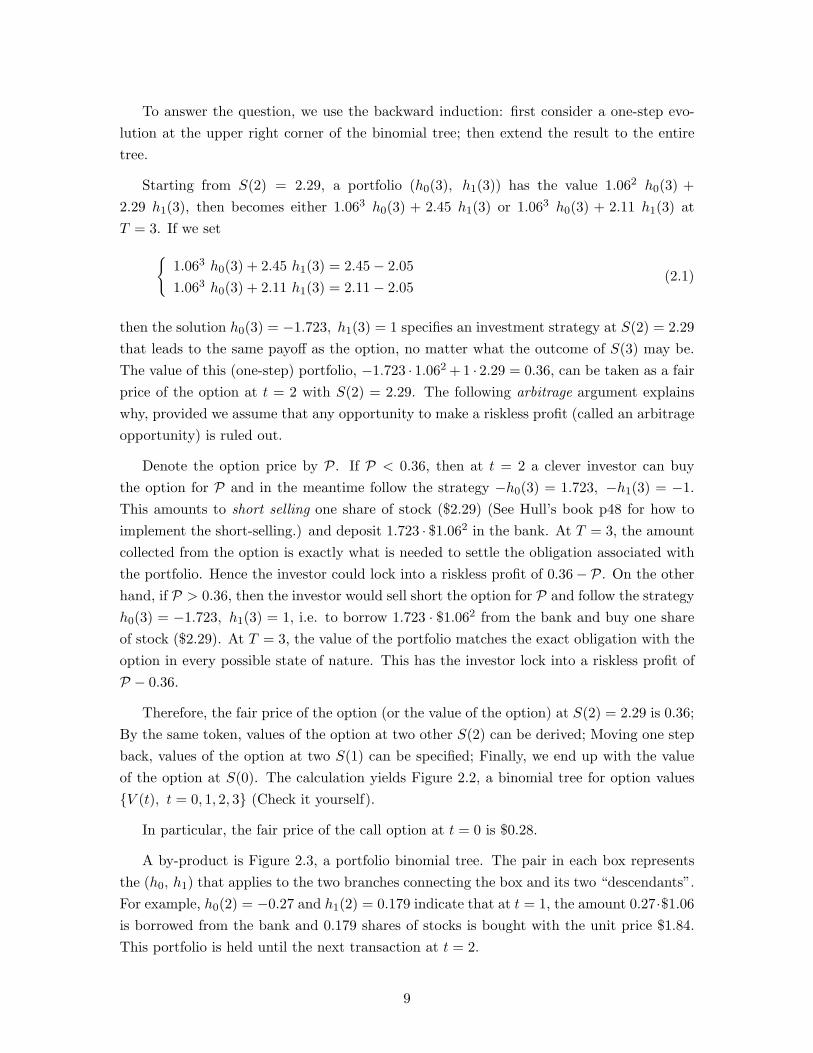
To answer the question, we use the backward induction: first consider a one-step evo-lution at the upper right corner of the binomial tree; then extend the result to the entiretree.
Starting from S(2) = 2.29, a portfolio (h0(3), h1(3)) has the value 1.062 h0(3) +2.29 h1(3), then becomes either 1.063 h0(3) + 2.45 h1(3) or 1.063 h0(3) + 2.11 h1(3) atT = 3. If we set
1.063 h0(3) + 2.45 h1(3) = 2.45− 2.051.063 h0(3) + 2.11 h1(3) = 2.11− 2.05
(2.1)
then the solution h0(3) = −1.723, h1(3) = 1 specifies an investment strategy at S(2) = 2.29that leads to the same payoff as the option, no matter what the outcome of S(3) may be.The value of this (one-step) portfolio, −1.723 · 1.062 + 1 · 2.29 = 0.36, can be taken as a fairprice of the option at t = 2 with S(2) = 2.29. The following arbitrage argument explainswhy, provided we assume that any opportunity to make a riskless profit (called an arbitrageopportunity) is ruled out.
Denote the option price by P. If P < 0.36, then at t = 2 a clever investor can buythe option for P and in the meantime follow the strategy −h0(3) = 1.723, −h1(3) = −1.This amounts to short selling one share of stock ($2.29) (See Hull’s book p48 for how toimplement the short-selling.) and deposit 1.723 · $1.062 in the bank. At T = 3, the amountcollected from the option is exactly what is needed to settle the obligation associated withthe portfolio. Hence the investor could lock into a riskless profit of 0.36−P. On the otherhand, if P > 0.36, then the investor would sell short the option for P and follow the strategyh0(3) = −1.723, h1(3) = 1, i.e. to borrow 1.723 · $1.062 from the bank and buy one shareof stock ($2.29). At T = 3, the value of the portfolio matches the exact obligation with theoption in every possible state of nature. This has the investor lock into a riskless profit ofP − 0.36.
Therefore, the fair price of the option (or the value of the option) at S(2) = 2.29 is 0.36;By the same token, values of the option at two other S(2) can be derived; Moving one stepback, values of the option at two S(1) can be specified; Finally, we end up with the valueof the option at S(0). The calculation yields Figure 2.2, a binomial tree for option valuesV (t), t = 0, 1, 2, 3 (Check it yourself).
In particular, the fair price of the call option at t = 0 is $0.28.
A by-product is Figure 2.3, a portfolio binomial tree. The pair in each box representsthe (h0, h1) that applies to the two branches connecting the box and its two “descendants”.For example, h0(2) = −0.27 and h1(2) = 0.179 indicate that at t = 1, the amount 0.27·$1.06is borrowed from the bank and 0.179 shares of stocks is bought with the unit price $1.84.This portfolio is held until the next transaction at t = 2.
9

V (0) = 0.28
©©©©©©*
HHHHHHj
V (1) = 0.31
©©©©©©*
HHHHHHj
V (1) = 0.04
©©©©©©*
HHHHHHj
V (2) = 0.36
©©©©©©*
HHHHHHj
V (2) = 0.05
©©©©©©*
HHHHHHj
V (2) = 0.00
©©©©©©*
HHHHHHj
V (3) = 0.40
V (3) = 0.06
V (3) = 0.00
V (3) = 0.00
Figure 2.2: Option value tree
10

−1.525, 0.9
©©©©©©*
HHHHHHj
−1.66, 0.969
©©©©©©*
HHHHHHj
−0.27, 0.179
©©©©©©*
HHHHHHj
−1.723, 1
©©©©©©*
HHHHHHj
−0.304, 0.2
©©©©©©*
HHHHHHj
0, 0
©©©©©©*
HHHHHHj
Figure 2.3: Portfolio tree
11

2.3 Risk neutral probabilities
More information can be extracted from this example. Let
q =1 + r − d
u− d=
1.06− 0.921.07− 0.92
=1415
, (2.2)
and denote by V (t, k) the value of the call option at the location (t, k). Note that thelocation of each box in this recombining tree is uniquely identified by a pair (t, k) withnt = k. Then we have
V (t, k) = (1 + r)−1 [ q V (t + 1, k + 1) + (1− q) V (t + 1, k) ]. (2.3)
Hence the value in each box is expressed as a discounted weighted average of the values inthe two descendent boxes. When the factors u, d and the rate r are constants over the treeas in this example, so is the weight q. Such a binomial tree is called a homogeneous tree.Later on we will demonstrate that the method extends to inhomogeneous trees also.
Hence we have two methods to price the call option: one by solving equations like (2.1)thus replicating the portfolio; the other by taking discounted weighted averages like (2.3).The impact is far-reaching. If we define
Q(ω) = qU(ω)(1− q)3−U(ω), (2.4)
where U(ω) represents the total number of up moves in the path ω, then Q is a probabilitymeasure on Ω, called a risk neutral probability measure, e.g. Q(ω3) = q2(1− q) = 0.058.
It is interesting to notice that the underlying Bernoulli probability p and the probabilitymeasure P were not relevant in the option pricing. It is the risk neutral probability factorq and measure Q that are useful. In general, p 6= q and P 6= Q. The probability measureQ is not a part of the model assumptions, but constructed from the market data — stocksand interest rates. In that sense, Q is an empirical measure.
Exercises:
2.1 Calculate the risk neutral probabilities Q(ωk), k = 1, . . . , 8.
2.2 Check whether the weighted averages produce the same results in option pricing as inFigure 2.2. Some discrepancies may be due to rounding errors.
2.3 If we change the interest rate from 6% to 8%, what would happen? Can you still carryout all the calculation? Why?
12

Chapter 3
Arbitrage and Risk Neutral
Probability Measures
Several important concepts were illustrated in the example in Lecture 2:
• arbitrage;
• risk neutral probability measures;
• contingent claims such as call options;
• two different ways to price a contingent claim.
Now begin our general studies on these topics. Lecture 3 concerns the equivalence be-tween no arbitrage and the existence of risk neutral probability measures. In Lecture 4,we will demonstrate the valuation of a contingent claim by replicating portfolios or takingconditional expectations with respect to a risk neutral probability measure (or called anequivalent martingale measure).
3.1 Some economic considerations
An arbitrage opportunity is said to exist if there is a self-financing strategy h whose valuefunction satisfies
(a) V (0) = 0;
(b) V (T ) ≥ 0;
(c) P (V (T ) > 0) > 0.
13

Although a smart investor may seek and grab such a riskless way of making a profit, itwould only be a transient opportunity because once more people jump in, the prices of thesecurities would change and the equilibrium would break down. Hence from the economicstandpoint, we assume no arbitrage.
Example 3.1 In the example in Lecture 2, suppose the constant interest rate is 8%. Thenan arbitrage opportunity can be found easily. Just do nothing at t = 0 and t = 1, and shortsell one share of stock at t = 2, deposit the proceeds in the bank account. This enablesthe investor to make a net profit at T = 3. (Fill in the detail and convince yourself thisstrategy is self-financing.)
Example 3.2 Let the interest rate equal 7%. The situation is similar to but slightly moreinteresting than Example 3.1. Try to find an arbitrage strategy.
In general, it is not easy to check directly whether an arbitrage opportunity exists. Auseful criterion is given via equivalent martingale measures.
Assume the finite sample space Ω, the filtration FF as in Lecture 1. A stochastic processX = X(t), t = 0, 1, . . . , T is called a martingale under a probability measure Q on Ω andwith respect to FF , if the conditional expectation
EQ (X(t) | Ft−1) = X(t− 1) ∀ t = 1, . . . , T.
Sometimes we call X a Q-martingale. See Lawler’s book, Chap. 5 for the basic discussionon conditional expectations and martingale. The main result in Lecture 3 is
Theorem 3.1 No arbitrage ⇐⇒ there is a probability measure Q with Q(ω) > 0 ∀ω ∈ Ω,such that every discounted price process S∗n = S∗n(t), t = 0, 1, . . . , T is a Q-martingale,n = 1, . . . , N . Such a measure Q is called an equivalent martingale measure (EMM).
Results of this kind are sometimes referred to as fundamental theorems of asset pricing. Wefollow the approach due to Harrison and Pliska given in their seminal paper (1981, Stoch.Proc. and Their Appl. 11, 215-260).
3.2 Proof of Theorem 3.1: sufficiency “⇐=”
This is an easy direction. It suffices to verify that G∗(t) is Q-martingale [so is V ∗(t) by(1.11)]. Note that by (1.9), for every t = 1, . . . , T , the conditional expectation under Q is
E [∆G∗(t) | Ft−1] =N∑
n=1
E [hn(t)∆S∗n(t) | Ft−1] =N∑
n=1
hn(t) E [∆S∗n(t) | Ft−1] = 0.
14

The second equality follows from that hn is predictable, and the third equality is due tothat S∗n is a martingale. It is useful to realize that for each n, the process
Xn(t) =t∑
u=1
hn(u) ∆S∗n(u)
is also a martingale, as the result of the transform from the martingale S∗n(t) via thepredictable process hn.
3.3 Proof of Theorem 3.1: necessity “=⇒”
A contingent claim is a random variable Y that represents the payoff at time T from a seller(short position) to a buyer (long position). Recall that the sample space Ω = ω1, . . . , ωK.Hence the set of possible values Y (ω1), . . . , Y (ωK) of a contingent claim Y can be consideredas an element in RRK . Let
G = Y ∈ RRK , Y = G∗(T ) for some trading strategy h;
A = Y ∈ RRK , Y ≥ 0 and Y (ω) > 0 for some ω ∈ Ω;
and
G⊥ = Z ∈ RRK , Y · Z = 0 ∀ Y ∈ G.
Note that G is a linear subspace of RRK (why?), and G⊥ is its orthogonal complement.A is the (closed) first quadrant (excluding the origin). No arbitrage implies G ∩ A = ∅.Furthermore, let
W = Y ∈ RRK , Y ≥ 0, Y1 + . . . + YK = 1,
which is a closed convex subset of A. It follows from the Separating Hyperplane Theoremthat there exists λ ∈ G⊥ such that λ · Y > 0 for all Y ∈ W. (See Pliska’s book p14and Duffie’s book p275 for more details.) This implies λ(ω) > 0 for all ω ∈ Ω. Define aprobability measure
Q(ω) =λ(ω)∑ω′ λ(ω′)
, ω ∈ Ω.
It follows from Q ∈ G⊥ that for any predictable process h,
EQ
[N∑
n=1
T∑
t=1
hn(t) ∆S∗n(t)
]= 0.
15

Hence for every n and any predictable process hn,
EQ
[T∑
t=1
hn(t) ∆S∗n(t)
]= 0.
This implies that every S∗n is a Q-martingale (why?).
Notes:
(1) The above λ is called a state price vector. More on this later.
(2) Q is called an EMM because Q is equivalent to P , i.e. for every ω ∈ Ω, Q(ω) > 0 if and
only if P (ω) > 0.
16

Chapter 4
Risk Neutral Valuation of
Contingent Claims
A contingent claim Y introduced in Lecture 3 is a contract between a seller and a buyer.Since the seller promises to pay the buyer the amount Y at time T , the buyer normallypays some money to the seller at a certain time t < T , when they make the agreement.
Q1: What is the appropriate time t value of this contingent claim Y ? Is it well-defined?
Throughout Lecture 4 we assume no arbitrage. A contingent claim Y is said to bemarketable or attainable if there exists a self-financing trading strategy h whose value at T
satisfies V (T ) = Y . In this case, h is said to replicate or generate Y .
Q2: Under what conditions on the market, every contingent claim is marketable?
The next two sections answer Q1 and Q2 respectively.
4.1 Law of one price and risk neutral valuation principle
The law of one price is said to hold if there do not exist two trading strategies, say h and h′
with corresponding value processes denoted by V (t) and V ′(t), such that V (T ) = V ′(T )but V (t) 6= V ′(t) for some t < T . In other words, if the law of one price holds, then thereis no ambiguity about the time t value of any marketable claim at any time t.
Proposition 4.1 No arbitrage =⇒ the law of one price holds.
Proof By Theorem 3.1, there is an EMM Q such that all discounted price processesS∗n, n = 1, . . . , N , thus the discounted value process V ∗(t), are Q-martingales. HenceProposition 4.1 follows (why?).
17
The converse of Proposition 4.1 is not necessarily true.
Example 4.1 Revisit Example 3.2. With r = 0.07, the equation (2.2) yields q = 1. Inthis case, there is a degenerate probability measure Q defined on Ω with Q(ω1) = 1 andQ(ωk) = 0 for all k 6= 1. Note that Q is not an EMM. But we can still use the equation(2.3) to obtain all values. More generally, the law of one price remains true (why?).
Exercise 4.1 Construct another counterexample in a single period model (T = 1).
The following principle is the basis for asset pricing.
Risk neutral valuation principle: Assuming no arbitrage, the time t value of a mar-ketable contingent claim Y is equal to V (t), the time t value of the portfolio that replicatesY . Moreover,
V ∗(t) = EQ [Y/B(T ) | Ft], t = 0, 1, . . . , T (4.1)
for any EMM Q.
Exercise 4.2 Justify this principle.
4.2 Complete markets
The example in Lecture 2 illustrates that for a given contingent claim Y , its marketabilitycan be checked by solving a system of linear equations, step by step backwards. Such atedious procedure is worthwhile because it yields a replicating portfolio when Y is mar-ketable.
Instead of dealing with each individual claim, an alternative approach is to define com-plete markets: a market is said to be complete if every claim in the market is attainable. Ageneral criterion is:
Theorem 4.1 An arbitrage-free market is complete ⇐⇒ there is a unique EMM Q.
Proof
“=⇒” Assuming completeness, every contingent claim Y satisfies Y = V (T ) for someself-financing strategy h. Suppose Q1 and Q2 are two EMMs with the corresponding ex-pectations denoted by E1(·) and E2(·).
E1 [Y/B(T )] = E1 V ∗(T ) = E1V∗(0) = V ∗(0), (4.2)
where the second equality is due to that V ∗(t) is a Q1-martingale, and the last equality
18

follows from F0 = ∅, Ω. By the same token,
E2 [Y/B(T )] = V ∗(0). (4.3)
Hence E1 [Y/B(T )] = E2 [Y/B(T )]. This implies Q1 = Q2 since Y is arbitrary.
“⇐=” Assume the market is arbitrage-free but incomplete, and let C be the set of allmarketable contingent claims. Note that C is a linear subspace of RRK . Thus there existsa contingent claim Y ′ ∈ C⊥, with respect to the inner product (X, Y ) = EQ (XY ) on RRK
where Q is an EMM. Define
Q′(ω) =
[1 +
Y ′(ω)2 supω∈Ω |Y ′(ω)|
]Q(ω), ω ∈ Ω. (4.4)
Then
(i) Q′ is a probability measure since EQY ′ = 0;
(ii) Q′(ω) > 0 ∀ω and Q′ 6= Q;
(iii) Q′ is an EMM because for every n and any predictable process hn,
EQ′
[T∑
t=1
hn(t) ∆S∗n(t)
]= 0.
Exercise 4.3 Construct an example of arbitrage-free but incomplete single period model.
19
Chapter 5
Binomial Trees: a General Setting
In the next couple of lectures, we will extend the example in Lecture 2 to a general setting— binomial trees, as an important model for a single risky security. It has been extensivelyused by practitioners in pricing various kinds of derivatives of stocks or bonds. Historically,the model was proposed independently by Cox/Ross/Rubinstein (1979, J. Fin. Econ. 7,229-263) and Rendleman/Bartter (1979, J. Fin. 34, 1093-1110), although it was oftenreferred to as the CRR model.
5.1 The basic binomial tree model
The evolution of a risky security, say stock, is represented by S = S(t), t = 0, 1, . . . , T.Starting from a initial positive constant price S(0), assume in each time period the stockprice either goes up by a factor u > 1 with probability p, or goes down by a factor 0 < d < 1with probability 1 − p. The moves over time are iid Bernoulli random variables. For eacht, S(t) = S(0)untdt−nt , where nt represents the number of up moves up to t.
The bank account process B is deterministic with B(0) = 1 and a constant interest rate0 < r < 1. Hence B(t) = (1 + r)t.
The filtration FF is taken as the one generated by the history of S. The sample spaceΩ contains K = 2T different paths. The underlying probability P is defined by P (ω) =pU(ω)(1−p)T−U(ω), where U(ω) represents the total number of up moves in the path ω. Weassume 0 < p < 1 so that P (ω) > 0 ∀ω ∈ Ω.
As for EMMs, we have the following
Proposition 5.1 There exists a unique EMM Q ⇐⇒ d < 1 + r < u. In this case,
Q(ω) = qU(ω)(1− q)T−U(ω), with q =1 + r − d
u− d. (5.1)
20

Proof Let ξt = nt−nt−1. Then for every t, S∗(t) = S∗(t−1) (1+r)−1uξtd1−ξt . Therefore,
EQ [S∗(t) | Ft−1] = S∗(t− 1)
⇐⇒ u Q(ξt = 1 | nt−1) + d [1−Q(ξt = 1 | nt−1)] = 1 + r
⇐⇒ Q(ξt = 1 | nt−1) =1 + r − d
u− d,
where Q(ξt = 1 | nt−1) denotes the conditional probability (under Q) that the next moveis up given nt−1 up moves up to time t − 1. We can denote this (constant) conditionalprobability by q since it does not depend on t or nt−1. This implies that ξ1, . . . , ξT areiid Bernoulli random variables, and the martingale measure Q is given by (5.1). Note that0 < Q(ω) < 1 for every ω if and only if 0 < q < 1 if and only if d < 1 + r < u. The aboveargument also shows such an EMM Q is unique.
Corollary 5.1 The binomial tree model is a complete market.
5.2 Option pricing using binomial trees
A European option is a contingent claim such that the owner of the option may choose (butwith no obligation) to exercise it at an expiry or expiration time T and receive the paymentY from the writer of the option. Naturally, the option should be exercised if and only if thepayment is positive.
In the simplest case, the contingent claim is expressed as Y = g(S(T )) with somefunction g. Using (4.1) in the binomial tree model, the pricing formula for a Europeanoption at time t = 0, 1, . . . , T − 1 is given by
V (t) =1
(1 + r)T−t
T−t∑
k=0
(T − t
k
)qk(1− q)T−t−k g(S(t)ukdT−t−k). (5.2)
Here are some examples.
Example 5.1 Call options. g(S(T )) = (S(T ) − c)+ where c > 0 is called the exerciseprice or strike price. A special case was given in Lecture 2. Note that S(t)ukdT−t−k − c >
0 ⇐⇒ k > log (c/(S(t)dT−t))log (u/d) . Let k∗ be the smallest k such that this inequality holds. If
k∗ > T − t, then V (t) = 0. If k∗ ≤ T − t, then (5.2) becomes
V (t) = S(t)T−t∑
k=k∗
(T − t
k
)bk(1−b)T−t−k− c
(1 + r)T−t
T−t∑
k=k∗
(T − t
k
)qk(1−q)T−t−k,(5.3)
where b = qu/(1 + r) ∈ (0, 1) (why?). The nice thing about this formula is that it involvestwo sums of T − t− k∗ + 1 binomial probabilities.
21
Exercise 5.2 Put options. Set g(S(T )) = (c−S(T ))+. The owner of this option normallychooses to sell the stock at T for the strike price c if S(T ) < c (thus make the profit c−S(T )),or chooses not to exercise the option if S(T ) ≥ c. A pricing formula similar to (5.3) can bederived easily.
Note: Denote by ct and pt respectively, the time t values of the European call and putoptions with the same expiry T and exercise price c. Since (S(T ) − c)+ − (c − S(T ))+ =S(T )− c, we have the following put-call parity
ct − pt = S(t)− c
(1 + r)T−t. (5.4)
Example 5.3 Chooser options. A chooser option is an agreement that the owner of theoption has the right to choose at a fixed decision time T0 < T whether the option is to bea call or a put with a common exercise price c and remaining time to expiry T − T0. Todetermine the time t value of the chooser option (t ≤ T0), notice that the payoff at T is
(S(T )− c)+IA + (c− S(T ))+IAc = (c− S(T ))+ + IA (S(T )− c),
where the event A = cT0 > pT0, Ac is the complement of A, and IA is the indicator of A.By the put-call parity, cT0 − pT0 = S(T0)− c (1 + r)−(T−T0), which leads to A = S(T0) >
c (1 + r)−(T−T0). Therefore, the time T0 value of the chooser option is given by
(1 + r)−(T−T0)EQ [(c− S(T ))+ + IA (S(T )− c) | FT0 ]
= pT0 + IA EQ
[S(T )− c
(1 + r)T−T0
∣∣∣∣ FT0
]
= pT0 + IA
[S(T0)− c
(1 + r)T−T0
]
= pT0 +[S(T0)− c
(1 + r)T−T0
]+
.
Introducing the notation C(t, T, c) (resp. P (t, T, c)) for the time t value of a call (resp. put)option with the expiry T and exercise price c, then for any t = 0, 1, . . . , T0, the time t valueVch(t) of the chooser option can be represented as
Vch(t) = P (t, T, c) + C(t, T0, c (1 + r)−(T−T0)
), (5.5)
or equivalently (why?) as
Vch(t) = C(t, T, c) + P(t, T0, c (1 + r)−(T−T0)
). (5.6)
Exercise 5.1 Verify (5.5) and (5.6).
22

Chapter 6
The Black-Scholes Option Pricing
Formula
We will show in Lecture 6 that the celebrated Black-Scholes formula in option pricing canbe derived from the binomial option pricing formula through an asymptotic argument,provided the parameters in the binomial model are specified appropriately.
Fix T > 0, a real number. For a positive integer n, partition the interval [0, T ) into[(j − 1)T/n, jT/n), j = 1, . . . , n. The previous notation S(j) in the binomial model nowrepresents the stock price at time jT/n. Similarly, B(j) represents the bank account at timejT/n. Let rn = rT/n be the interest rate, where r > 0 is thought of as the instantaneousrate with the continuous compounding, since limn→∞(1 + rn)n = erT . Let an = σ
√Tn
where σ > 0 is interpreted as the instantaneous volatility. Set the up and down factors byun = ean(1 + rn) and dn = e−an(1 + rn). Note that dn < 1 for sufficiently large n.
The risk neutral probability, as n →∞, has the asymptotic expression
qn =1 + rn − dn
un − dn
=1− e−an
ean − e−an
=an − 1
2 a2n + o(a2
n)2an + 1
3a3n + o(a3
n)
=12− 1
4an + o(an),
where the notation o(ε) with ε > 0 means o(ε)/ε → 0 as ε → 0.
Recall the iid Bernoulli random variables ξj , j = 1, . . . , n introduced in Lecture 5, withQ(ξj = 1) = qn. The stock price at T is represented as
S(n) = S(0) uξ1+···+ξnn dn−(ξ1+···+ξn)
n .
23

Hence the value of the put option at time 0 is given by
p(n)0 = (1 + rn)−n EQ (c− S(n))+ = EQ
(c
(1 + rn)n− S(0) eYn
)+
, (6.1)
where
Yn =n∑
j=1
Yn,j =n∑
j=1
log
(u
ξjn d
1−ξjn
1 + rn
). (6.2)
Note that for fixed n, Yn,1, . . . , Yn,n are iid random variables with
EQ Yn,j = qn logun
1 + rn+ (1− qn) log
dn
1 + rn=−12
a2n + o(a2
n), (6.3)
EQ Y 2n,j = a2
n, (6.4)
and
EQ |Yn,j |m = o(a2n) ∀ m = 3, 4, . . . . (6.5)
Using characteristic functions [see the note after (6.8)], it follows that Yn converges indistribution to N(−σ2T/2, σ2T ) as n → ∞. It is noteworthy that the family Yn,j isa triangular array, hence the asymptotic distribution of Yn need not always belong to theGaussian distribution family. In other words, the argument here goes somewhat beyondthe basic form of “Central Limit Theorem”.
Since
|p(n)0 − EQ
(c e−rT − S(0) eYn
)+ | ≤ c |(1 + rn)−n − e−rT |, (why?) (6.6)
we have
limn→∞ p
(n)0
= limn→∞EQ
(c e−rT − S(0) eYn
)+
=∫ ∞
−∞e−z2/2
√2π
[c e−rT − S(0) exp
(−σ2T
2+ σ
√Tz
)]+
dz
= c e−rT Φ(−v2)− S(0) Φ(−v1),
where v1 = log(S(0)/c)+(r+σ2/2) T
σ√
T, v2 = v1 − σ
√T = log(S(0)/c)+(r−σ2/2) T
σ√
T, and Φ is the
cumulative distribution function of N(0, 1).
24

This is the Black-Scholes pricing formula for a European option. We choose to considerput options first since their payoff (or loss) functions are bounded which make the asymp-totic argument easier. The following pricing formula for a call option can be derived usingput-call parity:
limn→∞ c
(n)0 = S(0) Φ(v1)− c e−rT Φ(v2).
Furthermore, by changing 0 to any t ∈ (0, T ) and T to T − t, the same argument goesthrough, which provides the Black-Scholes formulas for pricing the time t value C(t, T ) ofa (European) call option:
C(t, T ) = S(t) Φ(v1)− c e−r(T−t)Φ(v2), (6.7)
and the time t value P (t, T ) of a (European) put option:
P (t, T ) = c e−r(T−t)Φ(−v2)− S(t) Φ(−v1), (6.8)
where v1 = log(S(t)/c)+(r+σ2/2) (T−t)
σ√
T−tand v2 = v1 − σ
√T − t = log(S(t)/c)+(r−σ2/2) (T−t)
σ√
T−t.
Note: To verify that Yn converges in distribution to N(−σ2T/2, σ2T ) as n →∞, considerthe characteristic function EQ eiwYn of Yn where w ∈ RR and i =
√−1 (imaginary unit incomplex analysis). Following the fact that Yn,1, . . . , Yn,n are iid, and (6.3) — (6.5), we havethe Taylor expansion
EQ eiwYn =n∏
j=1
EQ eiwYn,j
=
(1 + iwEQYn,j − w2
2EQY 2
n,j −iθ3
3!EQY 3
n,j
)n
−→ exp (−iwσ2T/2− w2σ2T/2)
as n → ∞, where θ satisfies |θ| ≤ |w|. Note that exp (−iwσ2T/2 − w2σ2T/2) is just thecharacteristic function of N(−σ2T/2, σ2T ).
Exercise 6.1 Derive the formula (6.7).
25

Chapter 7
American Options as Optimal
Stopping Problems
An American option is a contract between two parties made at a certain time t such thatthe buyer of the contract has the right, but not the obligation, to exercise the option atany time τ with t ≤ τ ≤ T . If the option is exercised at τ , then the seller pays the buyeran amount Y (τ) ≥ 0. For instance, Y (τ) = (S(τ) − c)+ for an American call option andY (τ) = (c− S(τ))+ for an American put option based on a single stock. One can identifyan American option by its payoff process Y A = Y (t), t = 0, 1, . . . , T. American optionsenjoy the additional flexibility — possibility of exercising earlier than T — compared totheir European option counterparts. What is the value V A(t) of an American option?
7.1 A special case: “American = European”
Since the holder of an American option can always choose not to exercise the option untiltime T , V A(t) ≥ V (t) where V (t) is the time t value of the European option with the payoffY = Y (T ). Nevertheless, there are situations where the two value processes coincide.
Proposition 7.1 Consider an American option Y A and the corresponding European optionwith time T value Y = Y (T ). If V (t) ≥ Y (t) for all t, then V (t) = V A(t) for all t, and itis optimal to wait until time T to exercise.
Proof For the holder of an American option, exercising at t only ends up with payoff Y (t),while selling the corresponding European option (or shorting the portfolio which replicatesthe European option) would guarantee you a time t payoff V (t). Hence the option shouldnot be exercised at t. Since t is arbitrary, it is optimal to wait until T to decide whether toexercise.
26
Consider the American call option with Y (t) = (S(t)− c)+ at each t where c = 2.05 inthe example given in Lecture 2. Proposition 7.1 applies to this case. See Figure 7.1.
Note: The fact that an American call option is equivalent to its European counterpart isdue to its special probability structure. We will discuss this later.
7.2 Optimal stopping
Section 7.1 is not a typical case. You may check the American put option in the sameexample. For instance, when S(2) = 1.69, an immediate exercise gives you the payoff2.05− 1.69 = 0.36, compared to the value of the corresponding European put:1.06−1
[1415 (2.05− 1.81) + 1
15 (2.05− 1.56)]
= 0.24 < 0.36. Hence postponing the exercisedecision until T is suboptimal (why?).
To study when it is optimal to exercise an American option and evaluate the option, weneed to introduce supermartingales, submartingales and stopping times.
A stochastic process X = X(t), t = 0, 1, . . . , T is called a Q-supermartingale under aprobability measure Q on Ω and with respect to FF , if the conditional expectation
EQ (X(t) | Ft−1) ≤ X(t− 1) ∀ t = 1, . . . , T ;
On the other hand, X is called Q-submartingale if
EQ (X(t) | Ft−1) ≥ X(t− 1) ∀ t = 1, . . . , T.
All martingales are both supermartingales and submartingales, but not vice versa. Recallthat the discounted value process of a European option is a Q-martingale under an EMM Q.It turns out that the discounted value process of an American option is a Q-supermartingale.
A stopping time τ is a random variable taking values in the set 0, 1, . . . , T ;∞ suchthat for every t ≤ T , the event τ = t ∈ Ft, i.e. the information on whether τ = toccurs is available at time t. As a simple example, suppose the stock price S(0) = 2, thenτ1 = mint : S(t) > 2.1 is a stopping time, but τ2 = maxt : S(t) > 2.1 is not a stoppingtime. We allow stopping times to take the value ∞ in order to represent some events ofinterest that never occur up to time T .
An American option Y A is said to be marketable if for every stopping time τ ≤ T thecontingent claim Y (τ) can be replicated. Here is a basic result for American option pricing.
Theorem 7.1 For an EMM Q, define a stochastic process Z = Z(t), t = 0, 1, . . . , T
27

V (0) = 0.28
Y (0) = 0.00
©©©©©©©*
HHHHHHHj
V (1) = 0.31
Y (1) = 0.09
©©©©©©©*
HHHHHHHj
V (1) = 0.04
Y (1) = 0.00
©©©©©©©*
HHHHHHHj
V (2) = 0.36
Y (2) = 0.24
©©©©©©©*
HHHHHHHj
V (2) = 0.05
Y (2) = 0.00
©©©©©©©*
HHHHHHHj
V (2) = 0.00
Y (2) = 0.00
©©©©©©©*
HHHHHHHj
V (3) = 0.40
Y (3) = 0.40
V (3) = 0.06
Y (3) = 0.06
V (3) = 0.00
Y (3) = 0.00
V (3) = 0.00
Y (3) = 0.00
Figure 7.1: Exercise at t or T?
28

iteratively via the dynamic programming equations
Z(T ) = Y (T )Z(t) = max Y (t), EQ [Z(t + 1)B(t)/B(t + 1) | Ft] , t ≤ T − 1.
(7.1)
Then
(a) For each t,
Z(t) = maxτ
EQ [Y (τ)B(t)/B(τ) | Ft], (7.2)
where the maximum is over all stopping times t ≤ τ ≤ T .
(b) The maximum on the RHS of (7.2) is attained by the stopping time
τ(t) = min t′ ≥ t : Z(t′) = Y (t′). (7.3)
(c) The discounted version Z∗ of Z is the smallest Q-supermartingale satisfying
Z(t) ≥ Y (t) ∀t. (7.4)
(Z is called the Snell envelope of Y A.)
(d) For a marketable American option Y A, its value process is given by
V A(t) = Z(t) ∀t, (7.5)
and the optimal (early) exercise strategy at time t is given by the stopping time τ(t).
Proof
For (a) and (b), use backward induction. (7.2) and (7.3) clearly hold for t = T . Suppose(7.2) holds for t, then
Z(t− 1)
= max Y (t− 1), EQ[Z(t)B(t− 1)/B(t) | Ft−1]= max Y (t− 1), EQmax
τ≥tEQ[Y (τ)B(t)/B(τ) | Ft] B(t− 1)/B(t) | Ft−1
≥ max Y (t− 1), EQEQ[Y (τ)B(t)/B(τ) | Ft] B(t− 1)/B(t) | Ft−1= max Y (t− 1), EQ[Y (τ)B(t− 1)/B(τ) | Ft−1]
for any stopping time τ ≥ t. Hence
Z(t− 1)
≥ max Y (t− 1), maxτ≥t
EQ[Y (τ)B(t− 1)/B(τ) | Ft−1]≥ max
τ≥t−1EQ[Y (τ)B(t− 1)/B(τ) | Ft−1] (why?).
29

On the other hand, assuming (7.3) for t leads to
Z(t− 1)
= max Y (t− 1), EQ[Z(t)B(t− 1)/B(t) | Ft−1]= max Y (t− 1), EQEQ[Y (τ(t))B(t)/B(τ(t)) | Ft] B(t− 1)/B(t) | Ft−1= max Y (t− 1), EQ[Y (τ(t))B(t− 1)/B(τ(t)) | Ft−1]= EQ[Y (τ(t− 1))B(t− 1)/B(τ(t− 1)) | Ft−1] (why?)
≤ maxτ≥t−1
EQ[Y (τ)B(t− 1)/B(τ) | Ft−1].
Therefore, (7.2) and (7.3) have been verified for t− 1.
For (c), it follows from (7.1) that Z∗ is a Q-supermartingale and Z(t) ≥ Y (t) for all t.Suppose U is another process such that U∗ is a Q-supermartingale and U(t) ≥ Y (t) for allt. Then
U(t− 1) ≥ max Y (t− 1), EQ[U(t)B(t− 1)/B(t) | Ft−1] t = 1, . . . , T − 1. (7.6)
Starting from U(T ) ≥ Y (T ) = Z(T ) and working backwards iteratively in (7.6) and (7.1)will lead to U(t) ≥ Z(t) for all t.
For (d), we use an arbitrage argument (or called hedging) as follows.
Suppose V A(t) > Z(t). Then one can sell the option for V A(t) and take a portfolioreplicating Y (τ(t)) at the cost Z(t) and invest V A(t) − Z(t) in the bank account. Later,if the buyer exercises the option at some time τ ≤ τ(t), you liquidate the portfolio, collectZ(τ) and pay the buyer Y (τ). These transactions guarantee you a positive profit. On theother hand, if the buyer does not exercise by ξ = τ(t) < T , then you repeat this process:take a portfolio replicating Y (τ(ξ)) at the cost EQ[Z(ξ + 1)B(ξ)/B(ξ + 1) | Fξ], which isat most Z(ξ) = Y (ξ) by (7.1). As before, if the buyer exercises at some time τ ≤ τ(ξ),then the value of the portfolio will be enough to cover the payoff Y (τ). If the buyer doesnot exercise by τ(ξ), then you repeat the process once again, etc. The basic fact is thatyou always have enough money in the portfolio to cover the needed payoff, and you overallprofit will be at least V A(t)− Z(t) > 0.
For the opposite case V A(t) < Z(t), you can reverse the strategy: buy the option forV A(t), take the negative of the previous portfolio, collect Z(t) and invest the differenceZ(t)− V A(t) in the bank account. Later you exercise the option at time τ(t) and liquidatethe replicating portfolio at the same time. Since V (τ(t)) = Y (τ(t)), the amount you collectfrom the option seller is exactly equal to your liability on the portfolio. In the mean time,you have [Z(t)− V A(t)] B(τ(t))/B(t) > 0 in your bank account.
Therefore, there would be an arbitrage opportunity if V A(t) 6= Z(t). Moreover, (7.3)specifies an optimal exercise strategy for the American option buyer, because other strategies
30

would run the possible risk of exercising when Z(τ) > Y (τ) at some time τ . In that case,the buyer would sacrifice the amount Z(τ)− Y (τ) > 0.
We have thus far completed the proof of Theorem 7.1.
Exercise 7.1 Construct a binomial tree for the American put option values and theoptimal exercise times in the example given in Lecture 2.
31

Chapter 8
More on Valuation of American
Options
8.1 “American calls = European calls”
Yes, the above quote is really true, i.e. American calls have the same values as theirEuropean counterparts in the simple set-up given in Lecture 7, thus there should be noearlier exercises. This is because Y ∗(τ) is a submartingale.
Proposition 8.1 If Y ∗(τ) is a Q-submartingale for a marketable American option Y A,then for every t = 0, 1, . . . , T , the optimal exercise strategy is just τ(t) = T , and V A(t) =V (t), where V (t) is the time t value of the European option with terminal payoff Y (T ).
Proof
V A(t)
= EQ[Y (τ(t))B(t)/B(τ(t)) | Ft]
=T∑
s=t
EQ
[Y (s)B(t)/B(s) Iτ(t)=s
∣∣∣ Ft
]
≤T∑
s=t
EQ
EQ
[Y (T )B(t)/B(T ) Iτ(t)=s
∣∣∣ Fs
] ∣∣∣ Ft
= EQ[Y (T )B(t)/B(T ) | Ft]
= V (t).
Corollary 8.1 In the set-up given in Lecture 7, there should be no exercise earlier than T
for an American call option.
32
Proof To check Y ∗(t) is a submartingale, note that for every t = 1, . . . , T ,
EQ[(S∗(t)− c /B(t))+ | Ft−1]
≥ EQ[S∗(t)− c /B(t) | Ft−1]
= S∗(t− 1)− c EQ[1/B(t) | Ft−1]
≥ S∗(t− 1)− c /B(t− 1).
Since EQ[(S∗(t)− c /B(t))+ | Ft−1] ≥ 0, we have EQ[(S∗(t)− c /B(t))+ | Ft−1] ≥[S∗(t− 1)− c /B(t− 1)]+.
Note: It is a crucial part of the proof of Corollary 8.1 that S∗ is a Q-martingale, which isnot the case in the next section.
8.2 Options on a dividend-paying stock
In a more realistic market, some dividend-paying stocks may issue cash payments, calleddividends, to shareholders on a periodic basis. A dividend is referred to as the reductionin the stock price on the ex-dividend date. There may be several ex-dividend dates in astock, and possibly many different forms of dividends. For illustration, we consider thebinomial tree in Lecture 2 again, where T = 3 is the only ex-dividend date and the dividendis issued as a constant yield λ of the stock. This means the shareholder will receive adividend payment at T which amounts to either λuS(T − 1) or λdS(T − 1) according tothe stock fluctuation. In the meantime, the ex-dividend stock price at time T will be either(1− λ)uS(T − 1) or (1− λ)dS(T − 1). This corresponds to the traditional assumption thatthe stock price declines on the ex-dividend date by the dividend amount. One can easilycomplete this modified binomial tree.
Various options (calls, puts, and others; European or American) on dividend-payingstocks can be priced virtually in the same way as before, except that the exercise payoffis identified as [(1 − λ)uS(T − 1) − c]+ or [(1 − λ)dS(T − 1) − c]+ for calls, etc. In thissituation, the methodology using binomial trees enjoys its great flexibility.
This example also shows that on a dividend-paying stock, an American call need nothave the same value as its European counterpart. Corollary 8.1 does not hold for Americancall options on dividend-paying stocks. To see this, consider the inequality
(1 + r)[S(T − 1)− c]+
> q [(1− λ)uS(T − 1)− c]+ + (1− q) [(1− λ)dS(T − 1)− c]+, (8.1)
which amounts to 1.06 (2.29−2.05) > 1415 [(1−λ)2.45−2.05]+ + 1
15 [(1−λ)2.11−2.05]+ whenS(2) = 2.29, thus λ > 0.05 leads to exercising at t = 2.
33

Another simple form of dividend is “known dollar dividend” (see Hull’s book p354).
34
Chapter 9
Return and Risk
One of the important problems in modern financial economics is the quantification of thetrade-off between risk and expected return. Although common sense suggests that riskyinvestments such as stocks will generally yield higher returns than riskless investments, itwas the development of the Capital Asset Pricing Model (CAPM) that enables economiststo quantify risk and the reward for bearing it. The CAPM implies that the expected returnof an asset must be linearly related to the covariance of the its return with the return ofthe market portfolio.
We will introduce the concepts of return and risk, then discuss some basic versions ofCAPM.
9.1 Return processes
In the basic set-up in Lecture 1, assume a constant interest rate r(t) ≡ r for simplicity. Foreach n = 1, . . . , N , define the corresponding return process Rn = Rn(t) by Rn(0) = 0,and for t = 1, . . . , T ,
Rn(t) =
∆Sn(t)/Sn(t− 1), if Sn(t− 1) > 0
0, if Sn(t− 1) = 0.(9.1)
Also, R0(t) ≡ r for the bank account.
It is easy to see that for t = 1, . . . , T ,
Sn(t) = Sn(0) +t∑
v=1
Sn(v − 1)Rn(v), (9.2)
35

and
Sn(t) = Sn(0)t∏
v=1
[1 + Rn(v)]. (9.3)
What is the relation between Rn and R∗n, which is the return process corresponding to
S∗n? Note that
∆S∗n(t) = Sn(t)/B(t)− S∗n(t− 1)
=Sn(t− 1) [1 + Rn(t)]
(1 + r)t− S∗n(t− 1)
= S∗n(t− 1)Rn(t)− r
1 + r,
and ∆S∗n(t) = S∗n(t− 1) R∗n(t) by definition. Hence
R∗n(t) =
Rn(t)− r
1 + r. (9.4)
Now we define the return process R = R(t) of a portfolio h as the return correspondingthe value process V for h: R(0) = 0 and for t = 1, . . . , T ,
R(t) =
∆V (t)/V (t− 1), if V (t− 1) > 0
0, if V (t− 1) ≤ 0.(9.5)
If we let R∗ be the return process corresponding to V ∗, i.e. defined as in (9.5) with V
replaced by V ∗, then
R∗(t) =R(t)− r
1 + r. (9.6)
Furthermore, since V (t)− V (t− 1) = h0(t)∆B(t) +∑N
n=1 hn(t)∆Sn(t), we have
R(t) =
[h0(t)(1 + r)t−1
V (t− 1)
]r +
N∑
n=1
[hn(t)Sn(t− 1)
V (t− 1)
]Rn(t), (9.7)
which expresses the return for the portfolio as a linear combination of the returns for theindividual securities. In this expression, hn(t)Sn(t−1)
V (t−1) represents the fraction of the investor’swealth invested in security n at time t− 1 and about to be carried forward to time t.
9.2 Risk premium (single period)
The original version of CAPM is a single period model. To illustrate the basic idea, weintroduce the risk premium in a single period model (T = 1) first, and then extend it tothe multi-period case later.
36

For ω ∈ Ω, the ratio L(ω) = Q(ω)/P (ω) is called the state price density (or stateprice deflator), where P and Q denote the underlying probability measure and an EMMrespectively (i.e. we assume no arbitrage). Write Rn(1) = Rn for each n, and R(1) = R.Note that
EQ
(Rn − r
1 + r
)= 0. (9.8)
Hence the covariance
cov(Rn, L) = EP (RnL)− EP Rn EP L = EQRn − EP Rn = r −EP Rn.
Thus the difference EP Rn − r, called the risk premium for security n, is expressed as
EP Rn − r = − cov(Rn, L). (9.9)
Normally this is positive since investors usually believe that the expected returns of riskysecurities are higher than the riskless return r.
Following (9.7) with t = 1, we have
EP R− r = − cov(R, L). (9.10)
Consider a class of marketable contingent claims of the form a + bL where a and b aretwo constants with b 6= 0. Any such a claim is perfectly correlated with the state pricedeflator L. Suppose h′ is the strategy replicating a+bL whose value and return are denotedby V ′ and R′ respectively. Then a + bL = V ′(1) = V ′(0)(1 + R′). Thus
cov(R, L) =V ′(0)
bcov(R, R′).
Hence (9.10) becomes
EP R− r = −V ′(0)b
cov(R, R′). (9.11)
Setting h = h′ (note that h is an arbitrary portfolio) turns (9.11) to
EP R′ − r = −V ′(0)b
var(R′). (9.12)
Using this to substitute for V ′(0)b in (9.11), we obtain
Proposition 9.1 Let R′ be the return of a marketable contingent claim a + bL and R thereturn of an arbitrary portfolio h. Then
EP R− r = βh (EP R′ − r), (9.13)
37

where βh = cov(R, R′)var(R′) is called the beta of the trading strategy h with respect to the trading
strategy h′ that replicates a + bL.
(9.13) is referred to as a state price beta model, showing that the risk premium of a portfoliois proportional to the risk premium of a portfolio perfectly correlated with a state pricedeflator, where the proportional constant is the associated regression coefficient.
Note: Recall that the unique best linear predictor (to minimize the mean squared error)of Y based on X is given by Y = EY + β (X − EX) where β = cov(X, Y )/var(X).
38
Chapter 10
Optimal Portfolios
In the next couple of lectures, we will study optimization of portfolios, its connection withCAPM. It is noticeable that while only an EMM Q is relevant in option pricing, both theunderlying probability measure P and the EMM Q play an important role in this part ofthe studies.
10.1 Optimal portfolios
The objective in a basic optimal portfolio problem is to maximize the expected utility oftime T wealth, assuming there is no consumption before T .
Let U(w) represent the utility of wealth w at time T and assume the function U isdifferentiable, concave and strictly increasing. Here is a basic problem:
(P1) Find a self-financing strategy h with V (0) = w0 (a given initial wealth) to maximizeE U(V (T )), where E(·) denotes the expectation with respect to P .
The following problem is equivalent to (P1):
(P2) Find predictable processes h1, . . . , hN to maximize E U(B(T ) [w0 + G∗(T )]).
The reason that (P2) is equivalent to (P1) is this: for a solution (h1, . . . , hN ), it is easy tochoose h0 such that h = (h0, h1, . . . , hn) is self-financing with V (0) = w0.
Before solving (P2), notice that if there exists an arbitrage opportunity, then therecannot exist an optimal portfolio as a solution to (P1) or (P2). In other words, we have
39
Proposition 10.1 If h is a solution to (P1) or (P2), then there exists an EMM given by
Q(ω) =P (ω) B(T ; ω) U ′(V (T ;ω))
E [B(T ) U ′(V (T ))], ω ∈ Ω (10.1)
where U ′(V (T )) = dU(w)dw
∣∣∣w=V (T )
.
Proof For any t, n and event A ∈ Ft−1, hn(t; ω) specifies the optimal trading position insecurity n carried forward from time t− 1 to time t when ω ∈ A, with other components ofh fixed. The first-order necessary condition for this restricted optimality is
∑
ω∈A
P (ω) U ′(B(T ; ω) [w0 + G∗(T ; ω)]) B(T ; ω)∆S∗n(t; ω) = 0,
thus E U ′(B(T ) [w0 + G∗(T )]) B(T )∆S∗n(t) | Ft−1 = 0, which impliesEQ [∆S∗n(t) | Ft−1] = 0 by (10.1).
10.2 Computation via dynamic programming
The computation involved in solving (P2) can be intensive, especially when T , N and K
are large. The usual calculus-based optimization procedure would be intractable. A moreefficient method is dynamic programming by which a multiperiod decision problem can bereduced to a sequence of single period problems, working backwards in time. To implementthis, let U(t, w) be the maximum expected utility of time T wealth given the current timet, the current wealth w, and the history Ft.
Starting from U(T,w) = U(w), it follows that for t = 0, 1, . . . , T − 1,
U(t, w) (10.2)
= max E
U
(t + 1, B(t + 1)
[w/B(t) +
N∑
n=1
hn(t + 1)∆S∗n(t + 1)
]) ∣∣∣∣∣ Ft
,
where the maximum is over Ft-measurable random variables h1(t + 1), . . . , hN (t + 1); andh0(t + 1) is chosen in a self-financing manner.
To illustrate this, consider the example in Lecture 2 in which we let p = 0.4 and set theutility U(w) = 1− e−w. The RHS of (10.2) becomes
maxh
E 1− exp [−1.06w − h (S(3)− 1.06 S(2))] | S(2) = 2.29= max
h1− exp(−1.06w) g(h)
= 1− exp(−1.06w) minh
g(h),
40

where
g(h) = 0.4 exp(−h(2.45− 1.06 · 2.29)) + 0.6 exp(−h(2.11− 1.06 · 2.29)),
and h ∈ RR (not the notation for the entire portfolio). Setting the derivative of g(h) withrespect to h equal to zero will lead to h = −8.96376. Plugging this back into g(h) will yieldthe maximal expected value U(2, w) conditioning on S(2) = 2.29.
Exercise 10.1 Complete the dynamic programming procedure for this example. Thinkabout how the value of w affects the result.
41

Chapter 11
Optimization via EMMs
In this lecture, we present an alternative method for solving (P1) or (P2) in Lecture 10,using an EMM Q. Later in this course, we will demonstrate this useful approach in someother problems, such as model calibration.
11.1 Basic approach
Assume the market is complete and let Cw0 be the set of time T contingent claims that canbe generated by some self-financing strategy starting with initial wealth w0. We can alsowrite
Cw0 = Y ∈ RRK : EQ [Y/B(T )] = w0.
The following problem is obviously equivalent to (P1) or (P2):
(P3) There are two parts:
(i) Maximize E U(Y ) subject to Y ∈ Cw0 ;
(ii) Find a self-financing strategy h to replicate the solution Y of (i).
Since we are familiar with Part (ii) already, we now consider Part (i) by introducing aLagrange multiplier λ and maximizing E U(Y ) − λ EQ [Y/B(T )]. Using the state pricedensity, this problem can be rewritten as maximizing the objective function
E [U(Y )− λ L Y/B(T )] =∑ω
P (ω) [U(Y (ω))− λ L(ω)Y (ω)/B(T ; ω)].
The necessary condition is that for each ω ∈ Ω,
U ′(Y (ω)) = λ L(ω)/B(T ; ω), (11.1)
42
thus
Y = (U ′)−1(λ L /B(T )), (11.2)
where (U ′)−1 represents the inverse function of U ′. Moreover, the correct value of λ ischosen to satisfy
EQ [(U ′)−1(λ L/B(T )) / B(T )] = w0. (11.3)
11.2 Examples
The following examples will show that to compute the optimal expected utility [(P3) Part(i)], the EMM approach is much more efficient than the dynamic programming introducedin Lecture 10. This is because the optimal portfolio has to be found before calculating theoptimal expected utility when using dynamic programming. While using the EMM “Divide-and-Conquer” method, the optimal expected utility is identified via an intermediate variableY which has a much smaller dimensionality compared to h. Although finding the optimalportfolio h [(P3) Part (ii)] still involves a significant amount of calculation, it is in a familiarterritory — asset pricing. We will derive the optimal solution Y in each example, then findthe optimal expected utility and the optimal portfolio in one example, and leave the otherexamples to the reader.
Example 11.1 For the exponential utility U(w) = 1− e−w, we have (U ′)−1(z) = − log z,z > 0. Hence (11.2) and (11.3) imply
Y = − log[L/B(T )] + [E(L/B(T ))]−1 w0 + E [L/B(T ) log(L/B(T ))]. (11.4)
Example 11.2 For the logarithmic utility U(w) = log w, w > 0, we have (U ′)−1(z) = 1/z,z > 0. Hence
Y = w0 B(T )/L. (11.5)
Example 11.3 For the quadratic utility U(w) = βw − w2/2 where β is a constant, wehave (U ′)−1(z) = β − z. Hence
Y = β +L
B(T )w0 − β E [L/B(T )]
E [L/B(T )]2. (11.6)
More concrete formulas can be obtained in a binomial tree model with the parametersu, d, r and p. The state price density
L = Q/P =(
q
p
)nT(
1− q
1− p
)T−nT
43

is a likelihood ratio, where q = (1 + r − d)/(u− d), and nt is the total number of up movesup to t. The optimal Y in Example 11.2 is given by
Y = w0 (1 + r)T(
p
q
)nT(
1− p
1− q
)T−nT
, (11.7)
and the optimal expected utility is
E U(Y ) = log w0 + T log(1 + r) + pT logp
q+ (1− p)T log
1− p
1− q. (11.8)
Furthermore, to derive the optimal portfolio h, we again work backwards and set
(1 + r)T h0(T ) + S(T − 1)u h1(T ) = w0(1 + r)T(
p
q
)nT−1+1 (1− p
1− q
)T−nT−1−1
(1 + r)T h0(T ) + S(T − 1)d h1(T ) = w0(1 + r)T(
p
q
)nT−1(
1− p
1− q
)T−nT−1
,
which yields
h1(T ) =w0(1 + r)T
(pq
)nT−1(
1−p1−q
)T−nT−1−1(p− q)
S(T − 1)(u− d) q(1− q); (11.9)
and
h0(T ) =w0
(pq
)nT−1(
1−p1−q
)T−nT−1−1[u(1− p)q − d(1− q)p]
(u− d) q(1− q). (11.10)
Since V (T − 1) = (1 + r)T−1h0(T ) + S(T − 1)h1(T ), it follows that
V (T − 1) = w0 (1 + r)T−1(
p
q
)nT−1(
1− p
1− q
)T−1−nT−1
, (11.11)
and the fraction of money invested at time T − 1 in the stock is given by
S(T − 1)h1(T )V (T − 1)
=(1 + r)(p− q)
(u− d) q(1− q). (11.12)
Notice that the RHS in (11.12) does not depend on nT−1 and T , also V (T − 1) in (11.11)has the same form as V (T ) = Y in (11.7). This means that the optimal trading strategy atany time and any state is simply to invest the fraction (1+r)(p−q)
(u−d) q(1−q) of the present wealth inthe stock.
Other examples need not enjoy such simplicity but can also be worked out.
44

Chapter 12
The Binomial Capital Asset
Pricing Model
Assume the binomial tree model with parameters u, d, r and p. For each t = 0, 1, . . . , T ,denote the conditional expectations EP (·|Ft) by Et(·) and EQ(·|Ft) by Et;Q(·). The corre-sponding conditional variance and covariance under P are denoted by vart and covt respec-tively. We first consider the mean-variance portfolio problem
(P4) For an arbitrarily fixed t = 0, 1, . . . , T − 1, minimize vartR(t + 1) subject toEtR(t + 1) = µt, where µt is a constant satisfying µt ≥ r and the portfolio returnR(t + 1) is defined by (9.5), or by (9.7),
R(t + 1) =
[h0(t + 1)(1 + r)t
V (t)
]r +
[h1(t + 1)S(t)
V (t)
]R1(t + 1).
Note that if µt = r, then vartR(t + 1) = 0 where R is simply the return of the portfoliocontaining the bank account only. Hence we assume µt > r.
The main result in this lecture is
Proposition 12.1 If R′ is a solution of (P4) and R is the return of an arbitrary portfolio,then
EtR(t + 1)− r = βt [EtR′(t + 1)− r], (12.1)
where βt = covt(R(t+1), R′(t+1))vart(R′(t+1)) .
The proof of Proposition 12.1 has several steps.
Step 1. (P4) is equivalent to
45

(P5) Minimize vartV (t + 1) subject to EtV (t + 1) = w0(1 + µt) and V (t) = w0.
Step 2. Introducing a Lagrange multiplier β, (P5) is equivalent to
(P6) Maximize Et[β V (t + 1)− (1/2) V 2(t + 1)] subject to V (t) = w0.
To verify this, notice that (P6) is the same as minimizing
− Et[β V (t + 1)− (1/2) V 2(t + 1)]
=12
vartV (t + 1) +12
[EtV (t + 1)]2 − β EtV (t + 1)
=12
[vartV (t + 1)− 2β EtV (t + 1)] +12
[EtV (t + 1)]2,
where the first term matches the objective function for (P5) (with a Lagrange multiplierβ), while the second term is equal to 1
2 [w0(1 + µt)]2 due to the given constraint.
Step 3. Define the state price density up to time t by
Lt =(
q
p
)nt(
1− q
1− p
)t−nt
,
and the “one-step state price density” between t and t + 1 by
lt+1 =Lt+1
Lt=
(q
p
)nt+1−nt(
1− q
1− p
)1−(nt+1−nt)
.
In the current context, lt+1 is a right version of state price density to use.
Following (11.6) in Example 11.3, the optimal solution of (P6) is given by
V (t + 1) = β − βlt+1
Et;Qlt+1+ w0(1 + r)
lt+1
Et;Qlt+1, (12.2)
which implies
EtV (t + 1) = β [1− (Et;Qlt+1)−1] + w0(1 + r) (Et;Qlt+1)−1.
Note that Et;Qlt+1 > 1 when p 6= q (by Jensen’s inequality). Therefore,EtV (t + 1) = w0(1 + µt) if and only if
β =w0[(1 + µt) Et;Qlt+1 − (1 + r)]
Et;Qlt+1 − 1. (12.3)
(12.3) specifies a relation between µt and β such that (P5) and (P6) are equivalent.
46

If we substitute (12.3) into (12.2) and calculate the corresponding return R(t + 1), wehave
R(t + 1) =µt Et;Qlt+1 − r
Et;Qlt+1 − 1− µt − r
Et;Qlt+1 − 1lt+1, (12.4)
which means the optimal solution of (P4) is of the form a + b lt+1. Hence Proposition 12.1follows from Proposition 9.1.
Note: Proposition 12.1 is a “look-ahead one step” result, which is essentially the same asa single period model. Nevertheless, the conditioning argument enables us to study thedynamics of a return process. It is also easy to extend the result to more general modelsthan binomial trees, provided the argument based on “conditional independence” still goesthrough.
47
Chapter 13
Cash Flows and Forward Prices
We like to broaden our studies in arbitrage pricing from options to other kinds of derivativesecurities in order to suit the need for quantitative analysis of the evergrowing financialmarket. Forward contracts, cash flows and their valuation will be considered in this lecture,and futures will be discussed in the next lecture. As you will see, some modifications of theprevious concepts and results are necessary although the basic principle still holds.
13.1 Dividends and returns
Assume the basic set-up in Lecture 1. In particular, the bank account B need not havea constant interest rate r(t) ≡ r. Such a general treatment will be useful later on whenconsidering fixed income securities.
A cash flow can be thought of as a contract which carries a value V (t) at time t becausethe buyer of the contract will receive cash payments from the seller in some future times.A good example of cash flows is the dividends associated with a stock that we mentionedin Section 8.2 without detailed discussion.
For n = 1, . . . , N and t = 0, 1, . . . , T , let Dn(t) be the dividend per unit of securityn issued at time t, in particular Dn(0) = 0. Let Sn(t) represent the ex-dividend price ofsecurity n, i.e. the price right after any time t dividend payment. Assume the dividendprocess is adapted. To check whether arbitrage opportunities exist, it is better to look atreturns rather than security prices.
Note that a holder of one unit of security n at time t−1 will earn a profit ∆Sn(t)+Dn(t)over the period (t − 1, t]. The definition of return process Rn = Rn(t) given in Section
48
9.1 is modified as follows: Rn(0) = 0, and for t = 1, . . . , T ,
Rn(t) =
∆Sn(t)+Dn(t)Sn(t−1) , if Sn(t− 1) > 0
0, if Sn(t− 1) = 0.(13.1)
Still, R0(t) = r(t) for the bank account. Moreover, the return process for S∗n is defined byR∗
n(0) = 0, and for t = 1, . . . , T ,
R∗n(t) =
∆S∗n(t)+Dn(t)/B(t)S∗n(t−1) , if S∗n(t− 1) > 0
0, if S∗n(t− 1) = 0.(13.2)
Also, R∗0(t) ≡ 0 for the bank account.
If X = X(t), t = 0, 1, . . . , T is a martingale under a probability measure Q andwith respect to FF , then the increment process ∆X = ∆X(t) is called the correspondingmartingale difference sequence, i.e.
EQ (∆X(t) | Ft−1) = 0 ∀ t = 1, . . . , T.
Here is a modification of Theorem 3.1 in the case of dividend-paying securities.
Theorem 13.1 No arbitrage ⇐⇒ there is a probability measure Q with Q(ω) > 0 ∀ω ∈ Ω,such that R∗
n = R∗n(t), t = 1, . . . , T is a Q-martingale difference sequence, n = 1, . . . , N .
We still call Q an EMM.
The proof of Theorem 3.1 still works if we replace ∆Sn(t) there by ∆Sn(t) + Dn(t).
13.2 Forward contracts and prices
A forward contract is an agreement made between two parties at time t in which the buyeragrees to buy an underlying asset on a certain specified future date τ (with t < τ ≤ T ) fora delivery price; while the seller agrees to sell the asset on the same date τ for the sameprice. At the maturity date τ , the seller delivers the asset to the buyer in return for acash payment equal to the delivery price. Although the assets in forward contracts can becommodities, we only focus on securities. The delivery price that would make the time t
value of the forward contract to either party zero is called the forward price, denoted byFO(t). A basic problem is to determine FO(t) for a forward contract.
Since we only consider those forward contracts that can be replicated by self-financingtrading strategies, we assume a complete market without loss of generality. Let S(t) be the
49

time t price of an underlying security, and bt,τ = EQ[B(t)/B(τ) | Ft]−1 where Q is anEMM. Then we have
FO(t) = S(t) bt,τ . (13.3)
Note: The forward price FO(t) of a forward contract is not the time t value of the forwardcontract. The time t value of the forward contract is zero.
There are a couple of ways to verify (13.3). One is to use risk neutral valuation. Noticethat the time τ value of the forward contract is S(τ)− FO(t). By the definition of FO(t),we should have EQ[S(τ)− FO(t)] B(t)/B(τ) | Ft = 0, hence
S(t) = EQ[S(τ) B(t)/B(τ) | Ft]
= EQ[FO(t) B(t)/B(τ) | Ft] = FO(t) EQ[B(t)/B(τ) | Ft],
which implies (13.3). The last equality is due to that FO(t) is measurable with respect toFt.
Another way to verify (13.3) is via the standard arbitrage argument. Technically, thatwould need a zero-coupon bond with maturity τ . Here we only present the argument in thespecial case of r(t) ≡ r thus bt,τ = (1+ r)τ−t. This simplification makes the argument moretransparent.
Suppose first FO(t) < S(t) bt,τ . An investor can take a long position in the forwardcontract, short the security at time t, and deposit the proceeds in the bank. At time τ , thesecurity is purchased under the term of the forward contract for FO(t), the short positionin the security is closed out, and a profit S(t) bt,τ − FO(t) > 0 is earned.
On the other hand, suppose FO(t) > S(t) bt,τ . Then an investor can borrow the amountS(t) at time t, buy the security, and take a short position in the forward contract. At timeτ , the security is sold under the term of the forward contract for FO(t). After using theamount S(t) bt,τ to repay the loan, a profit FO(t)− S(t) bt,τ > 0 is realized.
The above result can be generalized to the case of dividend-paying securities. Suppressthe subscript n in the notation given in Section 13.1 and denote the dividend process (acash flow) by D = D(t). At any fixed time s > t, D(s) is simply a contingent claim, thusits time t value is dt,s = EQ[D(s)B(t)/B(s) | Ft], called the time t present value of D(s).Following Theorem 13.1, we have
EQ[∆S∗(t + 1) + D(t + 1)/B(t + 1) | Ft] = 0 ∀t = 0, 1, . . . , T − 1; (13.4)
and for τ > t,
S∗(t) = EQ
τ∑
s=t+1
D(s)B(s)
+ S∗(τ)
∣∣∣∣∣∣Ft
. (13.5)
50
Hence the time t present value of a cash flow (such as dividends) D(s), t < s ≤ τ is givenby
τ∑
s=t+1
dt,s = S(t)− EQ[S(τ)B(t)/B(τ) | Ft]. (13.6)
Now we have
Proposition 13.1 With a security process S and a dividend process D, the time t for-ward price FO(t) of a forward contract, which is received and paid at time τ > t, is givenby
FO(t) =
S(t)−
τ∑
s=t+1
dt,s
bt,τ = EQ[S(τ)B(t)/B(τ) | Ft] bt,τ . (13.7)
Proof Once again, we start with the equation
EQ[S(τ)− FO(t)] B(t)/B(τ) | Ft = 0 (13.8)
that defines FO(t). But the ex-dividend price S does not satisfy
EQ[S(τ)B(t)/B(τ) | Ft] = S(t).
Instead, it follows from (13.6) that
EQ[S(τ)B(t)/B(τ) | Ft] = S(t)−τ∑
s=t+1
dt,s,
which matches FO(t) after multiplying both sides by bt,τ .
Alternatively, we may consider the following portfolio that replicates S(τ):
At time t: buy one unit of security for S(t);
Also at time t: for each s = t + 1, . . . , τ , borrow dt,s by undertaking the negative of thestrategy that replicates the time s receipt D(s), then at time s use the dividend paymentD(s) to settle the liability under the strategy.
The time t value of this replicating portfolio also amounts to
EQ[S(τ)B(t)/B(τ) | Ft] = S(t)−τ∑
s=t+1
dt,s.
Example 13.1 Consider the binomial model with parameters u, d, r, and a dividend issuedwith the constant yield λ on the ex-dividend date τ , where 1 ≤ τ ≤ T .
51

Suppose S(τ − 1) > 0, then (13.1) yields the return
R(τ) =∆S(τ) + D(τ)
S(τ − 1)= u− 1 or d− 1, (13.9)
which is the same as in the case without dividends. The same calculation reduces (13.2) to
R∗(τ) =u
1 + r− 1 or
d
1 + r− 1. (13.10)
According to Theorem 13.1, we can set
EQ[R∗(τ)|Fτ−1] = q
(u
1 + r− 1
)+ (1− q)
(d
1 + r− 1
)= 0, (13.11)
and obtain that q = 1+r−du−d which is the risk neutral probability provided d < 1 + r < u.
Therefore, the risk neutral probability q (thus the corresponding EMM Q) remains the sameas in the case without dividends.
Furthermore, (13.7) gives us the one-step forward price FO(τ−1) for a forward contractwith maturity τ :
FO(τ − 1) = S(τ − 1) (1 + r)(1− λ). (13.12)
Any contingent claim Y defined at τ has its time τ − 1 valueV (τ − 1) = (1 + r)−1EQ[Y |Fτ−1]. For example, given S(τ − 1) = ζ, the time τ − 1 value ofan European call option Y = [S(τ)− c]+ is given by
V (τ − 1) = (1 + r)−1q [u(1− λ)ζ − c]+ + (1− q) [d(1− λ)ζ − c]+. (13.13)
.
52

Chapter 14
Futures Contracts
14.1 Futures vs forward contracts
Like a forward contract, a futures contract is an agreement made at time t which involvesa cash payment between two parties in a specified future time with a specified deliveryprice. However, there are a number of noteworthy differences between futures and forwardcontracts that we summarize as follows. See Hull’s book for more details.
• Trading
Forward: Traded over-the-counter (OTC) anywhere anytime by telephone or othercommunications between individual buyers and sellers;
Futures: Traded on some centralized exchange floors, such as Chicago Board ofTrade (CBOT) and New York Futures Exchange (NYFE), during their businesshours.
• Standardization
Forward: Not standardized — almost everything in a contract is based on privatenegotiation: the underlying assets to be traded, price, delivery time and location,etc.
Futures: A standardized contract specifies the underlying asset to be traded, price,delivery date (chosen from among a limited number of dates each year) andlocation.
• Delivery
Forward: Delivery or final cash settlement usually take place.
Futures: A very small proportion of contracts are actually delivered. A majorityof contracts are closed out prior to maturity.
53

• Collateral and margin
Forward: Collateral level negotiable; no adjustment for daily price fluctuations,settlement only at end of contract. Hence market participants bear the risk ofcounter-party defaulting.
Futures: A central clearinghouse is associated with each exchange to regulate thetrade. Each investor is required to initiate a margin account as a security deposit.Positions in futures contracts are governed by a daily settlement procedure, re-ferred to as marking to market. The investor is allowed to withdraw any balancein the margin account in excess of the initial margin. To ensure that the balancein the margin account never becomes negative, a maintenance margin, which issomewhat lower than the initial margin, is set. If the balance in the marginaccount falls below the maintenance margin, the investor receives a margin calland is expected to top up the margin account to the initial margin level thenext day. The extra funds deposited are called a variation margin. A failure toprovide the variation margin would result in closing out the investor’s position,i.e. a broker associated with the clearinghouse would sell the contract.
• Information and liquidity (important to statistical analysis of financial market, sometimesreferred to as empirical finance)
Forward: No volume information available; low liquidity due to a large variety ofcontract terms.
Futures: Volume information published; high liquidity due to standardized con-tracts.
14.2 Futures prices
Marking to market is a device in futures market to reduce the risk of default inherent inforward contracts. Recall that the value of a forward contract need not equal zero except atthe time when the contract starts. In contrast, the value of a futures contract is maintainedat zero at all times via marking to market. Thus either party can close out his/her positionat any time.
The futures price of a futures contract, specified at the time when the futures contract isentered into, is not like the forward price which is defined by the equation (13.8). Instead,it is determined on a given futures exchange by the usual law of supply and demand, similarto stock prices.
For m = 1, . . . ,M , let FUm(t, tm) be the futures price of a futures contract with startingdate t and maturity date tm, and ∆FUm(s, tm) = FUm(s, tm)−FUm(s−1, tm), t < s ≤ tm.
54

An investor taking a long position either receives a payment ∆FUm(s, tm) at time s, ormakes a payment −∆FUm(s, tm) if the futures price falls. These fluctuations are reflectedin marking to market. We will study the connections between
(i) the futures price process FUm(·, tm) and the underlying security process Sm(·);(ii) the futures price FUm(t, tm) and the corresponding forward price FO(t) with the samematurity tm.
Let (h; hf ) = (h0, h1, . . . , hN ; hf1 , . . . , hf
M ) denote the portfolio process in a combinedspot/futures market, where all the components are predictable processes. For each m, hf
m(t)represents the position in futures contract m held from time t − 1 to t. We assume thatFUm(t, tm) = 0 and hf
m(t) = 0 for any t > tm.
Consider the value process. The time t value of a portfolio right before marking tomarket is
V (t) = h0(t)B(t) +N∑
n=1
hn(t)Sn(t) +M∑
m=1
hfm(t)∆FUm(t, tm); (14.1)
and the time t value of the portfolio right after marking to market is
V +(t) = h0(t + 1)B(t) +N∑
n=1
hn(t + 1)Sn(t). (14.2)
Compared to (14.1), the absence of terms involving futures prices in (14.2) is due to theupdating adjustment via marking to market. A trading strategy (h; hf ) is said to beself-financing if its value process satisfies
V (t) = V +(t) ∀ t = 1, . . . , T − 1. (14.3)
Since a futures trader must have positive wealth, we cannot define arbitrage by startingwith V (0) = 0. Nevertheless, other definitions of arbitrage would work. An arbitrageopportunity in a spot/futures market corresponds to a self-financing strategy (h; hf ) whosevalue satisfies
(a) V ∗(T ) ≥ V ∗(0) ∀ω, and
(b) V ∗(T ) > V ∗(0) for some ω.
An alternative to (a) and (b) is
(a′) G∗(T ) ≥ 0 ∀ω, and
(b′) G∗(T ) > 0 for some ω,
55

where the discounted gain G∗ is specified through its increment in (t− 1, t]
∆G∗(t) =N∑
n=1
hn(t)∆S∗n(t) +M∑
m=1
hfm(t)∆FUm(t, tm)/B(t), t = 1, . . . , T. (14.4)
The following theorem is an extension of Theorem 3.1 to the case of spot/futures market.
Theorem 14.1 For a combined spot/futures market, no arbitrage ⇐⇒ there is an EMMQ, such that for every n = 1, . . . , N , the process S∗n is a Q-martingale; moreover, for everym = 1, . . . M ,
EQ[∆FUm(t, tm)/B(t) | Ft−1] = 0, t = 1, . . . , T. (14.5)
The proof is left as an exercise, since the argument in proving Theorem 3.1 can bemodified straightforwardly.
Corollary 14.1 Consider the following special cases of Theorem 14.1.
(a) Suppose B is a predictable process. Then (14.5) is equivalent to that FUm(·, tm) is aQ-martingale for each m.
(b) Suppose B is deterministic with r(t) ≡ r. Then for every m and t,
FUm(t, tm) = FO(t), (14.6)
where FO(t) is the forward price of a forward contract starting at t and ending at tm.
Proof (a) is trivial. For (b), note that FUm(tm, tm) = Sm(tm), i.e. the futures priceconverges to the spot price of the underlying security at the delivery date. The martingaleproperties of FUm(·, tm) and Sm(·) imply that
FUm(t, tm) = EQ[FUm(tm, tm) | Ft] = EQ[Sm(tm) | Ft]
= (1 + r)tm−tSm(t) = FO(t).
Note: (14.6) remains valid when underlying securities pay dividends. This just followsfrom (13.7).
Example 14.1 For a single period market, (14.6) always holds even when B is random,adaptive and nonpredictable. This is intuitively obvious since there is no marking to market.The holder of a futures contract can only wait until the delivery date — same as in a similarforward contract. To verify (14.6), note that (14.5) in this case is written as
EQ[∆FUm(1, 1)/B(1) | F0] = EQ[Sm(1)− FUm(0, 1)]/B(1) | F0 = 0,
56

which is just the equation to define the forward price FO(0).
Example 14.2 Consider a binomial tree model with T = 2. Identify ω1 = uu, ω2 = ud,ω3 = du and ω4 = dd. Let S(0) = 1, u = 1.07, d = 0.92; B(0) = B(1) = 1 and
B(2) =
1.03, on ω1, ω21.04, on ω3, ω4
Since there is only a single stock, we suppress the subscript m, and calculate Q, FU(0, 2)and FO(0) (also with delivery date T = 2).
• To calculate Q, write EQ[S(t)/B(t) | Ft−1] = S(t− 1)/B(t− 1):
For t = 2:
1.07q1 + 0.92(1− q1) = 1.03 thus q1 = 1115 on ω1, ω2;
1.07q2 + 0.92(1− q2) = 1.04 thus q2 = 1215 on ω3, ω4.
For t = 1:
q0 = 1−du−d = 8
15 .
Hence Q(ωi), i = 1, 2, 3, 4, are equal to q0q1, q0(1− q1), (1− q0)q2 and (1− q0)(1− q2)respectively.
• (14.5) is carried out in two steps.
For t = 2, S(1)/B(1) = FU(1, 2) EQ[B−1(2) | F1], i.e.
FU(1, 2) = 1.07 · 1.03 = 1.1021 on ω1, ω2;FU(1, 2) = 0.92 · 1.04 = 0.9568 on ω3, ω4.For t = 1,
FU(0, 2) = EQFU(1, 2) = 1.1021q0 + 0.9568(1− q0) = 155144150000 ≈ 1.03429.
• (13.3) yields
FO(0) = S(0) [EQB−1(2)]−1 = [1.03−1q0 + 1.04−1(1− q0)]−1 = 160680155300 ≈ 1.03464.
In this example, B is random and predictable, but FU(0, 2) 6= FO(0).
14.3 Options on futures
Options or more general contingent claims can be defined as derivatives of underlying se-curities and/or futures in a combined spot/futures market. Risk neutral valuation basedon Theorem 14.1 can be carried out. Any marketable contingent claim can be hedged via
57

replicating portfolios (h; hf ). The only technical subtlety to keep in mind is that whenusing an EMM Q, the discounted security price S∗ is a Q-martingale while the undiscountedfutures price FU(·, τ) is a Q-martingale (assuming B is predictable). Hence the price of acontingent claim depends on whether it is defined as a derivative of a security or a futurescontract. We will give some related problems in Homework 3.
58

Chapter 15
Zero-coupon Bonds, Yields and
Forward Rates
The fixed-income market is an important part of the global financial market in which var-ious interest rate securities, such as bonds, are traded. The total volume of fixed-incomesecurities traded in the market is much greater than that of equities such as common stocks.Mathematical models for fixed-income derivatives are also more subtle and complex. Wewill introduce the basic concepts and some useful models in the next few lectures.
Assume the basic setting in Section 1.1: a sample space Ω, an underlying probabilitymeasure P , a filtration FF with finite horizon T . In particular, the bank account B isassumed to be random and predictable with interest rate r(t) > 0 for all t = 1, . . . , T . Thismeans that the riskless interest rate r(t) for borrowing or lending over the period (t− 1, t]is known at time t− 1. The process B is taken as a numeraire. r(t) is called the spot rateor short rate.
• Various bonds are considered as risky securities. One of them is a collection of zero-coupon or discount bonds, denoted by B(t, τ) : 0 ≤ t ≤ τ, τ = 1, . . . , T, whereB(t, τ) represents the time t price of a zero-coupon bond with maturity τ . Sometimeswe simply call a zero coupon bond with maturity τ a τ -bond. Assume that for eachτ , the process B(·, τ) is positive and adapted to FF , in particular, B(τ, τ) = 1 at par(the nominal value is $1 at maturity). On the other hand, for each t, the collectionB(t, τ), t < τ ≤ T is called the time t term structure of zero-coupon bond prices.Hence we are dealing with a process B(·, ·) with double indices, which makes theanalysis considerably more challenging.
Now we consider a couple of other term structures equivalent to B(t, ·), and we assumet ≤ τ .
• Let Y (t, τ) be the constant interest rate (or return) at which B(t, τ), when compounded
59

during (t, τ ], would reach $1 at time τ , called the yield to maturity, i.e.
B(t, τ) [1 + Y (t, τ)]τ−t = 1, (15.1)
or equivalently,
Y (t, τ) = [B(t, τ)]−1τ−t − 1. (15.2)
In particular, Y (t − 1, t) = r(t), the spot rate at one period before maturity. [Why?See (15.7).] For each t, the collection Y (t, τ), t < τ ≤ T is called the time t termstructure of interest rates or yield curve. The two term structures B(t, ·) and Y (t, ·)are equivalent.
• Let f(t, τ) be the “short rate” such that
(i) it is locked into at time t;
(ii) it is applied to the period (τ, τ + 1];
(iii) it is associated with a (τ + 1)-bond.
Then we have
B(t, τ + 1)B(t, τ)
[1 + f(t, τ)] = 1, (15.3)
or equivalently,
f(t, τ) =B(t, τ)
B(t, τ + 1)− 1. (15.4)
To see why this is true, assume there exists an EMM Q such that for every τ , thediscounted τ -bond process B∗(·, τ) is a Q-martingale, i.e.
B(t− 1, τ) = EQ[B(t, τ)B(t− 1)/B(t) | Ft−1], 1 ≤ t ≤ τ. (15.5)
Notice that in a fixed income market, zero coupon bonds play the same role as riskysecurities like common stocks in a stock market. We can consider a forward contracton a (τ +1)-bond, delivered at τ . According to (13.3), its forward price FO(t) at timet is given by
FO(t) = B(t, τ + 1) bt,τ =B(t, τ + 1)
EQ[B(t)/B(τ) | Ft]=
B(t, τ + 1)B(t, τ)
, (15.6)
where the last equality is due to that
B(t, τ) = EQ[B(t)/B(τ) | Ft]. (15.7)
In particular,
f(t, t) = r(t + 1). (15.8)
60

Exercise 15.1 Verify the following results:
B(t, τ) = EQ[(1 + r(t + 1)) · · · (1 + r(τ))]−1 | Ft; (15.9)
r(t) = B−1(t− 1, t)− 1; (15.10)
B(t, τ) =τ∏
s=t+1
[1 + f(t, s− 1)]−1; (15.11)
For every t, B(t, τ) is strictly decreasing in τ .
61

Chapter 16
Examples of Term Structure
Models
There are two different kinds of term structure models: spot rate models (short rate models,equilibrium models, etc.), in which initial term structures are outputs from the models; andyield curve models (forward rate models, no arbitrage models, etc.), in which initial termstructures are inputs to the models. Before general studies of these two approaches, weillustrate them in two simple examples respectively in this lecture.
In both examples, we assume T = 3, Ω = ωi, i = 1, 2, 3, 4, and the following partitionsthat generate the filtration FF :
P1 = ω1, ω2, ω3, ω4;
P2 = ω1, ω2, ω3, ω4;
and
P3 = ω1, ω2, ω3, ω4.
Example 16.1
• Start with a spot rate binomial tree, Figure 16.1, in which
r(1) = 0.04;
r(2) =
0.06 on ω1, ω2,0.03 on ω3, ω4;
62

r(1) = 0.04
©©©©©©*
HHHHHHj
r(2) = 0.06
©©©©©©*
-
r(2) = 0.03 -
HHHHHHj
r(3) = 0.07
r(3) = 0.05
r(3) = 0.04
r(3) = 0.02
Figure 16.1: Spot rate tree
63

and
r(3) =
0.07 on ω1,0.05 on ω2,0.04 on ω3,0.02 on ω4.
64

• By (15.10) B(t− 1, t) = [1 + r(t)]−1, we obtain that
B(0, 1) = 0.9615;
B(1, 2) =
0.9434 on ω1, ω2,0.9709 on ω3, ω4;
and
B(2, 3) =
0.9346 on ω1,0.9524 on ω2,0.9615 on ω3,0.9804 on ω4.
• At this point, we have some flexibility. We choose an EMM Q by assigning Q(ωi) = 1/4,i = 1, 2, 3, 4.
• It follows from (15.7) or (15.9) that
B(0, 2) = EQ[1/B(2)] =1
1.04· 12·(
11.06
+1
1.03
)= 0.9203,
B(0, 3) = EQ[1/B(3)]
=1
1.04· 14·(
11.06 · 1.07
+1
1.06 · 1.05+
11.03 · 1.04
+1
1.03 · 1.02
)= 0.8811,
and
B(1, 3) = EQ
1
[1 + r(2)] [1 + r(3)]
∣∣∣∣ F1
=
11 + r(2)
EQ
1
1 + r(3)
∣∣∣∣ F1
=
11.06 · 1
2
(1
1.07 + 11.05
)= 0.8901 on ω1, ω2,
11.03 · 1
2
(1
1.04 + 11.02
)= 0.9427 on ω3, ω4.
The result is summarized in Table 16.1.
ω B(0, 1) B(0, 2) B(1, 2) B(0, 3) B(1, 3) B(2, 3) Q
ω1 0.9615 0.9203 0.9434 0.8811 0.8901 0.9346 0.25
ω2 ∼ ∼ ∼ ∼ ∼ 0.9524 ∼ω3 ∼ ∼ 0.9709 ∼ 0.9427 0.9615 ∼ω4 ∼ ∼ ∼ ∼ ∼ 0.9804 ∼
Table 16.1: Data for Example 16.1. The notation ∼ represents the same number asabove.
65

A drawback of the approach used in Example 16.1 is that the initial (time 0) termstructure is derived from the model, thus need not be consistent with the given data (theinitial term structure data is available at time 0). An alternative approach is to model theentire family of yield curves conditioning on the given initial term structure.
Example 16.2
• Suppose the initial term structure is given by
B(0, 1) = 0.96 [thus r(1) = 0.0417],
B(0, 2) = 0.92,
and
B(0, 3) = 0.88.
• If we let Q(ωi) = 1/4, i = 1, 2, 3, 4 as in Example 16.1, there is still some flexibility inspecification of r(2) and r(3), or equivalently, B(t, ·), t = 1, 2. We will move forwardone period at a time.
• For t = 2, set r(2) = 0.06 on ω1, ω2. Then
B(0, 2) =1
1 + r(1)EQ
[1
1 + r(2)
],
i.e.
0.92 =1
1.0417· 12
[1
1.06+
11 + r(2)
],
which gives rise to
r(2) = 0.0274 on ω3, ω4.
Hence
B(1, 2) =1
1 + r(2)=
0.9434 on ω1, ω2,0.9733 on ω3, ω4.
• For t = 3, set
r(3) =
0.07 on ω1,0.05 on ω2,0.04 on ω3.
66

Notice the constraint
B(0, 3) =1
1 + r(1)EQ
1
[1 + r(2)] [1 + r(3)]
,
i.e.
0.88 =1
1.0417· 14
[1
1.06 · 1.07+
11.06 · 1.05
+1
1.0274 · 1.04+
11.0274
· 11 + r(3)
],
which implies
r(3) = 0.0238 on ω4.
Therefore,
B(2, 3) =1
1 + r(3)=
0.9346 on ω1,0.9524 on ω2,0.9615 on ω3,0.9768 on ω3.
Finally,
B(1, 3) =1
1 + r(2)EQ
[1
1 + r(3)
∣∣∣∣ F1
]
=
11.06 · 1
2
(1
1.07 + 11.05
)= 0.8901 on ω1, ω2,
11.0274 · 1
2
(1
1.04 + 11.0238
)= 0.9433 on ω3, ω4.
The result is summarized in Table 16.2.
ω B(1, 2) B(1, 3) B(2, 3) r(2) r(3) Q
ω1 0.9434 0.8901 0.9346 0.06 0.07 0.25
ω2 ∼ ∼ 0.9524 ∼ 0.05 ∼ω3 0.9733 0.9433 0.9615 0.0274 0.04 ∼ω4 ∼ ∼ 0.9768 ∼ 0.0238 ∼
Table 16.2: Data for Example 16.2. The notation ∼ represents the same number asabove.
Notes:
(a) In Example 16.2, one can first specify all B(·, ·) in a consistent manner without usingQ and r(·). Then Q and r(·) will be determined accordingly.
(b) In practice, trinomial trees or bushy trees with even more branches from each node areoften used to study multi-factor term structure models (later).
67
Chapter 17
Spot Rate Modelling via Markov
Chains and Stochastic Difference
Equations
We introduce two methods in modelling spot rates: Markov chains (MC) and stochasticdifference equations (SDE). Each method has its own advantage. MC makes use of binomialtrees, and SDE is naturally linked to models in continuous-time finance. Overall, MCprovides somewhat more general models than SDE.
17.1 Spot rate Markov chains
A stochastic process X = X(t), t = 0, 1, . . . , T is called a Markov chain with a statespace S if for every t = 0, 1, . . . , T − 1,
PX(t + 1) = xt+1 | X(s) = xs, 0 ≤ s ≤ t = PX(t + 1) = xt+1 | X(t) = xt
for all possible values xs ∈ S, 0 ≤ s ≤ t + 1. Several quantities of interest, such as the spotrate r(·) and the zero-coupon bond B(·, ·) can be modelled as Markov chains. A convenientway is to construct an underlying Markov chain X such that r(·), B(·, ·), etc. are definedas appropriate functions of X. For example, we let r(t + 1) = gt(nt) with a strictly positiveand increasing function gt for each t.
Let S = (t, nt) : nt = 0, 1, . . . , t; t = 0, 1, . . . , T, where nt denotes the number of upmoves up to t in the binomial tree in Figure 17.1. The precise meaning of nt is not crucial.It can be thought of as coding a number of exogenous factors that affects r(·), B(·, ·), etc. ina fixed income market. Assume that X is a Markov chain under an EMM Q, with transition
68

q(0, 0); r(1, 0)
©©©©©©©*
-
q(1, 1); r(2, 1)
©©©©©©©*
-
q(1, 0); r(2, 0)
©©©©©©©*
-
q(2, 2); r(3, 2)
©©©©©©©*
-
q(2, 1); r(3, 1)
©©©©©©©*
-
q(2, 0); r(3, 0)
©©©©©©©*
-
Figure 17.1: Binomial tree of Markov chain X and spot rate r
69

probabilities
q(t, nt) = QX(t + 1) = (t + 1, nt + 1) | X(t) = (t, nt)= 1−QX(t + 1) = (t + 1, nt) | X(t) = (t, nt),
i.e. nt+1 = nt + 1 or nt are the only allowable transitions. Since r(·) is predictable, thevalue of spot rate r(t + 1) applied to the period (t, t + 1] is known at time t, denoted byr(t + 1, nt).
Note that this formulation forces a recombining tree as shown in Figure 17.1, but thisbinomial tree is inhomogeneous in the sense that the transition probabilities q take differentvalues at different nodes.
A full specification of the model involves T (T + 1) parameters: one value of q and onevalue of r at each node, with total number of T (T + 1)/2 nodes (not counting the terminalnodes at T ). The following special case illustrates this.
Example 17.1 Assume q(t, nt) ≡ 12 ∀ (t, nt) ∈ S. Moreover, the initial term structure
B(0, τ), τ = 1, . . . , T adds T constraints. There are still T (T − 1)/2 parameters to bespecified [among T (T + 1)/2 values of r]. It is often useful to reparametrize the model byspecifying the spot rate volatilities
σ(t, nt) =√
q(t, nt) [1− q(t, nt)] logr(t + 2, nt + 1)
r(t + 2, nt)=
12
logr(t + 2, nt + 1)
r(t + 2, nt)(17.1)
for t = 0, 1, . . . , T − 2. [Is σ(t, nt) > 0 ∀ (t, nt)? Why?]
If we let B(t, nt; τ) denote the value of B(t, τ) at the state (t, nt), then (15.5) impliesthat
B(t, nt; τ) =q(t, nt) B(t + 1, nt + 1; τ) + [1− q(t, nt)] B(t + 1, nt; τ)
1 + r(t + 1, nt). (17.2)
17.2 Stochastic difference equations
Let the spot rate r be governed by the SDE
∆r(t + 1) = µ(t, r(t)) + σ(t, r(t)) εt, (17.3)
where µ is a real-valued function and σ a positive function; ∆r(t + 1) = r(t + 1) − r(t),and εt, t = 0, 1, . . . , T − 1 are iid random variables with Q(εt = 1) = Q(εt = −1) = 1
2 .Obviously, under Q the increment ∆r(t + 1) has the conditional mean µ(t, r(t)) and theconditional variance σ2(t, r(t)) given r(t).
70

To see the connections between SDE and MC, first consider a special case of MC inwhich q(t, nt) ≡ 1
2 ∀ (t, nt) ∈ S. Then the increments nt − nt−1 are iid Bernoulli randomvariables under Q thus we can set
εt = 2(nt − nt−1)− 1. (17.4)
The SDE (17.3) is expressed as
r(t + 1, nt−1 + 1)− r(t, nt−1) = µ(t, r(t, nt−1)) + σ(t, r(t, nt−1))
and
r(t + 1, nt−1)− r(t, nt−1) = µ(t, r(t, nt−1))− σ(t, r(t, nt−1)),
in which case µ and σ should satisfy
µ(t, r(t, nt−1)) =12
[r(t + 1, nt−1 + 1) + r(t + 1, nt−1)− 2r(t, nt−1)]
and
σ(t, r(t, nt−1)) =12
[r(t + 1, nt−1 + 1)− r(t + 1, nt−1)],
so that the spot rate r is governed by (17.3).
On the other hand, if r satisfies the SDE (17.3), then clearly r is a Markov chain.However, there are a number of more interesting and subtle questions to be answered:
Q1 Under what conditions on µ and σ, an underlying MC X can be represented by arecombining binomial tree as in Figure 17.1 such that r is defined by r(t + 1) = gt(nt)?
Q2 What functions µ and σ will assure a positive spot rate r defined via (17.3)?
Q3 What functions µ and σ will guarantee that the spot rate r defined via (17.3) satisfiesthe mean reversion property, i.e. r tends to decrease when it is above a threshold andincrease when it is below the threshold?
We will discuss these issues in the next couple of lectures when we study some well-knownspecial models.
71

Chapter 18
Vasicek, Cox-Ingersoll-Ross, and
Hull-White Models
Different expressions of the drift µ and volatility σ in the SDE (17.3)
∆r(t + 1) = µ(t, r(t)) + σ(t, r(t)) εt
lead to various spot rate models. In this lecture, we first consider time-homogeneous SDEsin which µ(t, r(t)) = µ(r(t)) and σ(t, r(t)) = σ(r(t)), i.e. the drift and volatility do notinvolve time t explicitly. We then study an inhomogeneous SDE in Hull-White model,along with Markov chains represented by binomial or trinomial trees.
18.1 Vasicek and CIR models
Consider the following special cases in which a, b, σ are all positive constants, and β is aconstant with 0 ≤ β ≤ 1.
Example 18.1 (Vasicek model) µ(t, r(t)) = a[b− r(t)], σ(t, r(t)) = σ.
Example 18.2 [Cox-Ingersoll-Ross (CIR) model] µ(t, r(t)) = a[b− r(t)],σ(t, r(t)) = σ
√r(t).
Example 18.3 (a more general class) µ(t, r(t)) = a[b− r(t)], σ(t, r(t)) = σ [r(t)]β.
A common feature of these models is the mean reversion property: the spot rate r
tends to decrease if r > b and increase if r < b. An advantage of CIR over Vasicek isits capability of enforcing positive values on r. To formulate the question more precisely,assume r(1) = x > 0 and let
τx = inf 2 ≤ t ≤ T : r(t) ≤ 0. (18.1)
72

The question is: under what conditions on the parameters a, b and σ in the SDEs forVasicek and CIR respectively, Q(τx ≤ T ) = 0 will be satisfied? Note that Q(τx ≤ T ) = 0and P (τx ≤ T ) = 0 are equivalent since Q is an EMM. Both imply that the values of r
remain positive in the whole process. It turns out that those conditions needed in CIR arequite mild and reasonable, but the conditions needed in Vasicek are too strict to be realistic.More on this later.
18.2 Hull-White model
In a very general form, Hull-White model can be expressed via the SDE
∆r(t + 1) = a(t) [b(t)− r(t)] + σ(t) [r(t)]β εt, (18.2)
where β ≥ 0 is still a constant, but a(t), b(t) and σ(t) are positive-valued deterministicfunctions. These functions greatly enhance modelling flexibility, e.g. the initial term struc-ture can be incorporated into a(t) and b(t). The condition on εt is often relaxed in thismodel, e.g. εt’s are independent with Q(εt = 1) = q(t) < 1 .
Under what conditions on functions a, b and σ, an underlying MC X can be representedby a recombining tree such that r is defined by r(t + 1) = gt(nt) (Q1 in Lecture 17)? Arecombining tree requires that starting from any node, a “up-down” combination (εt = 1and εt+1 = −1) and a “down-up” combination (εt = −1 and εt+1 = 1) should merge at thesame node. In other words, starting from r(t), these two combinations must arrive at thesame value of r(t + 2). Standard calculation turns this into the condition
σ(t + 1) = [1− a(t + 1)] σ(t) ∀ t, (18.3)
which also requires a(t) < 1 ∀t (for positive volatility).
Trinomial trees are often used in this situation to provide an extra degree of freedom.In a trinomial tree, three branches come out of each node: up, middle and down. There are2t+1 nodes at time t. The recombining assumption consists of “up-down = middle-middle= down-up”, “up-middle = middle-up” and “down-middle = middle-down”. The threepossible moves up, middle and down correspond to εt = 1, εt = 0 and εt = −1, with riskneutral probabilities Q(εt = 1) = Q(εt = −1) = q(t) < 1/2 and Q(εt = 0) = 1− 2q(t). Thesame argument shows that the recombining condition is still given by (18.3).
18.3 Refined lattice and SDE
So far in Lectures 17 and 18, the binomial (or trinomial tree) models and SDEs for spot rateshave fixed integer 1 as the span for both time increment and space increment. Refinement of
73

this is needed for more realistic models, especially for passing the limit to continuous-timefinance. To carry out this technical step, fix T > 0 and positive integer n, let δ = T/n be thetime increment and
√δ the space increment in the binomial or trinomial trees. Accordingly,
for j = 0, 1, . . . , n− 1, we let
rδ(j) = r(jδ), ∆rδ(j + 1) = rδ(j + 1)− rδ(j).
The functions µδ(j, rδ(j)), σδ(j, rδ(j)), aδ(j) and bδ(j) are defined in the same way. TheSDE (17.3) becomes
∆rδ(j + 1) = µδ(j, rδ(j)) δ + σδ(j, rδ(j))√
δ εj . (18.4)
Keep in mind that for a fixed δ (or n), the basic setting in Lecture 1 is still valid.However, if we let n →∞ (thus δ → 0), many complicated technical issues will need to betaken care of.
74

Chapter 19
Heath-Jarrow-Morton Approach
and Ho-Lee Model
Lectures 17 and 18 focused on modelling the spot rate r. The corresponding term structurescan be derived based on r. This method is relatively easy to implement. A drawback is thatit lacks the capability of modelling yields (or zero-coupon bond prices) with different matu-rities. For example, if one is interested in the spread between short and long term interestrates, those spot rate models would have difficulties to model such a feature explicitly.
An alternative approach, proposed by Heath, Jarrow and Morton (HJM), is to consideran entire yield curve as a state variable that evolves over time. In principle, one can modelany one of the three equivalent term structures: zero-coupon bond prices, yields and forwardrates. It is often convenient to work with forward rates. In this lecture, we start with thebasic notation in HJM set-up, followed by more detailed discussion on a special case of HJM— the Ho-Lee model, and show how some spot rate models are derived from Ho-Lee model.
19.1 HJM setting
Following the basic framework in Lecture 15, we extend the idea of binomial trees to the statespace consisting of yield curves. A given value of the time t term structure f(t, τ), t ≤ τ ≤T−1 may move “up” with a (risk neutral) probability q or “down” with probability 1−q toone of the two possible values of the time t+1 term structure f(t+1, τ), t+1 ≤ τ ≤ T−1.In general, q may depend on t and the value of time t state. Such a binomial tree need notbe recombining. To fix the notation for a binomial tree in this context, a typical node isdenoted by (t, k), where t = 0, 1, . . . , T − 1; k = 0, 1, . . . , 2t − 1. Let ftk be a possible valueof the time t term structure, which is a vector with components ftk(τ), t ≤ τ ≤ T − 1.In particular, ft+1,2k and ft+1,2k+1 are the two immediate “descendants” of ftk in the
75

binomial tree. The risk neutral (conditional) probabilities moving from the (t, k) to thenext generation (t + 1, 2k) or (t + 1, 2k + 1) are qtk and 1− qtk respectively.
Example 19.1 We use the data in Example 16.1 to illustrate the above notation. First,Table 19.1 contains forward rates calculated from Table 16.1 by using the formula (15.4).
ω f(0, 0) f(0, 1) f(0, 2) f(1, 1) f(1, 2) f(2, 2) Q
ω1 0.04 0.045 0.044 0.06 0.06 0.07 0.25
ω2 ∼ ∼ ∼ ∼ ∼ 0.05 ∼ω3 ∼ ∼ ∼ 0.03 0.03 0.04 ∼ω4 ∼ ∼ ∼ ∼ ∼ 0.02 ∼
Table 19.1: Forward rates in Example 16.1.
Next, the values ftk of the term structures are given as follows:
f00 = (f(0, 0), f(0, 1), f(0, 2)) on ω1, ω2, ω3, ω4 = (0.04, 0.045, 0.044)
f10 = (f(1, 1), f(1, 2)) on ω1, ω2 = (0.06, 0.06)
f11 = (f(1, 1), f(1, 2)) on ω3, ω4 = (0.03, 0.03)
f20 = f(2, 2) on ω1 = 0.07
f21 = f(2, 2) on ω2 = 0.05
f22 = f(2, 2) on ω3 = 0.04
f23 = f(2, 2) on ω4 = 0.02
There are two restrictions that a model builder must keep in mind in the specificationof term structures of forward rates: positivity of f(·, ·) and no arbitrage. It follows from(15.5), (15.8) and (15.11) that for τ = t + 2, . . . , T ,
τ∏
s=t+2
[1 + f(t, s− 1)]−1 = EQ
τ∏
s=t+2
[1 + f(t + 1, s− 1)]−1
∣∣∣∣∣∣Ft
. (19.1)
If the left-hand side is the value at a node (t, k), say, then we have
τ∏
s=t+2
11 + ftk(s− 1)
(19.2)
= qtk
τ∏
s=t+2
11 + ft+1,2k(s− 1)
+ (1− qtk)τ∏
s=t+2
11 + ft+1,2k+1(s− 1)
.
76

Example 19.2 For given f(t, t), . . . , f(t, T − 1), consider in each of the following threecases whether it is possible to specify positive values of ft+1,2k+1(t + 1), . . .,ft+1,2k+1(T − 1) such that (19.2) holds.
Case 1. Positive values ft+1,2k(t + 1), . . . , ft+1,2k(T − 1) and qtk ∈ (0, 1) are fixed;
Case 2. qtk ∈ (0, 1) is fixed, but there is flexibility in choosing positive valuesft+1,2k(t + 1), . . . , ft+1,2k(T − 1).
Case 3. Positive values ft+1,2k(t + 1), . . . , ft+1,2k(T − 1) are fixed, but there is flexibility inchoosing qtk ∈ (0, 1).
19.2 Ho-Lee model
The paper of Ho-Lee (Journal of Finance, 1986) proposed the first yield curve model, basedon which the general HJM was developed later on. In what follows, we first present Ho-Leemodel for the term structures of zero-coupon bond prices then turn it into the equivalentversion for forward rates, which enables us to see Ho-Lee model explicitly as a special caseof HJM setting in Section 19.1 and to connect Ho-Lee model to some short rate models.
A simple feature of Ho-Lee model is that it can be represented by a recombining binomialtree (a general HJM tree need not be recombining). Therefore, the notation in Section 19.1is modified to be adapted to the triangular lattice in Figure 17.1.
• On the triangle lattice (t, k) : k = 0, 1, . . . , t; t = 0, 1, . . . , T, the time t term structureB(t, τ), t < τ ≤ T assumes values Btk(τ), t < τ ≤ T.
• For t < τ ≤ T , let s = τ − t be the time to maturity, 1 ≤ s ≤ T − t. A perturbationfactor η(s) takes either the value u(s) > 1 (an “inflation” factor or a “up” move) withprobability q, or the value 0 < d(s) < 1 (a “deflation” factor or a “down” move) withprobability 1− q, where the (risk neutral) probability q is assumed to be a constant.The conditions
η(0) = 1 (19.3)
and
q u(s) + (1− q) d(s) = 1 ∀ 1 ≤ s ≤ T (19.4)
are satisfied.
• The evolution of time t term structure in (t, t + 1] follows
B(t + 1, τ) =B(t, τ)
B(t, t + 1)η(τ − t− 1), (19.5)
77

which can be spelled out as
Bt+1,k+1(τ) =Btk(τ)
Btk(t + 1)u(s− 1), (19.6)
or
Bt+1,k(τ) =Btk(τ)
Btk(t + 1)d(s− 1). (19.7)
• For t + 2 ≤ τ , a “up-down” combination gives rise to
Bt+2,k+1(τ) =Btk(τ)
Btk(t + 2)u(s− 1) d(s− 2)
u(1); (19.8)
while a “down-up” combination gives rise to
Bt+2,k+1(τ) =Btk(τ)
Btk(t + 2)d(s− 1) u(s− 2)
d(1). (19.9)
Therefore, the following “path-independent” condition that forces a recombining bi-nomial tree is needed:
u(s− 1) d(s− 2) d(1) = d(s− 1) u(s− 2) u(1). (19.10)
Using (19.4), we can simplify (19.10) as
1u(s− 1)
=θ
u(s− 2)+ q(1− θ) ∀ 2 ≤ s ≤ T, (19.11)
where θ is a constant, called the interest rate spread and given by
q + (1− q)θ =1
u(1), (19.12)
thus 0 < θ < 1. It follows from the induction and the condition u(0) = 1 that for0 ≤ s ≤ T ,
u(s) =1
q + (1− q)θs, (19.13)
and
d(s) =θs
q + (1− q)θs. (19.14)
• To sum up, the dynamics of term structures in Ho-Lee model is determined by twoconstant parameters q and θ, which makes Ho-Lee model computationally efficientbut also too restrictive (underparametrized). For instance, the zero-coupon bondprice may not always fall in the range [0, 1]. Still, Ho-Lee model plays a significantrole in modelling the entire yield curve. The state at node (t, k) (the time t yield curve)(Btk(t+1), Btk(t+2), . . . , Btk(T )) will change to (Bt+1,k+1(t+1), . . . , Bt+1,k+1(T )) atnode (t+1, k+1) with probability q, or (Bt+1,k(t+1), . . . , Bt+1,k(T )) at node (t+1, k)with probability 1− q.
78

• Note the relation
11 + f(t, τ)
=B(t, τ + 1)
B(t, τ). (19.15)
Following (19.6), (19.7), (19.13) and (19.14), the dynamics of forward rates is givenby
11 + ft+1,k+1(τ)
=1
1 + ftk(τ)q + (1− q)θτ−t−1
q + (1− q)θτ−t, (19.16)
or
11 + ft+1,k(τ)
=1
1 + ftk(τ)θ [q + (1− q)θτ−t−1]
q + (1− q)θτ−t. (19.17)
The state (ftk(t), ftk(t + 1), . . . , ftk(T − 1)) will turn to (ft+1,k+1(t + 1), . . . ,ft+1,k+1(T−1)) with probability q, or (ft+1,k(t+1), . . . , ft+1,k(T−1)) with probability1 − q. Compare this to Section 19.1, it can be seen clearly that Ho-Lee is a specialcase of HJM. In particular, Ho-Lee corresponds to a recombining binomial tree, andassumes a constant probability q at every node.
19.3 Spot rate models from Ho-Lee
In a binomial tree associated with Ho-Lee model, the recombining feature implies that thetotal number of “up’s” (or “down’s) determines the dynamics, regardless of their orders.Iterating (19.16) and (19.17) in t leads to
11 + ft,nt(τ)
=θt−nt
1 + f(0, τ)q + (1− q)θτ−t
q + (1− q)θτ, (19.18)
where nt represents the total number of “up’s” up to t. Set τ = t and recall (15.8), we have
r(t + 1) = [1 + f(0, t)] (qθ−t + 1− q) θnt − 1. (19.19)
The only random variable in (19.19) is nt which follows a binomial distribution.
79

Chapter 20
Forward Risk Adjusted Probability
Measures
Starting from this lecture, we will discuss valuation of interest rate derivatives. For aFτ -measurable contingent claim Y (τ), its time t value is given by
V (t) = EQ[Y (τ)B(t)/B(τ) | Ft] (20.1)
with a risk neutral probability measure Q. (20.1) is particularly convenient when the bankaccount process B is deterministic, because it simply becomes
V (t) = B(t)/B(τ) EQ[Y (τ) | Ft]. (20.2)
In the case of stochastic interest rate r, an alternative method is developed based on thefollowing change of measures.
For a fixed τ ≤ T , let M(τ) > 0 be a Fτ -measurable random variable satisfyingEQM(τ) = 1. Define a new probability measure P τ by
P τ (ω) = M(τ ; ω) Q(ω) ∀ω ∈ Ω. (20.3)
Obviously P τ is a probability measure and P τ (ω) > 0 for all ω. Let Eτ (·) denote theexpectation corresponding to P τ . Define a Q-martingale M = M(t) : t = 0, 1, . . . , τ by
M(t) = EQ[M(τ) | Ft].
Now we state a basic result of changing martingale measures.
Proposition 20.1 MY = M(t)Y (t) : t = 0, 1, . . . , τ is a Q-martingale if and only ifY = Y (t) : t = 0, 1, . . . , τ is a P τ -martingale.
80
Proof A major step is to show that
Eτ [M(t)Y (τ) | Ft] = EQ[M(τ)Y (τ) | Ft] ∀ t ≤ τ. (20.4)
To verify (20.4), take an arbitrary event A ∈ Ft. Then M(t) is constant on A and
M(t; ω) = EQ[M(τ)|A] =∑
ω′∈A
M(τ ; ω′)Q(ω′)/Q(A) = P τ (A)/Q(A) ∀ ω ∈ A.
Therefore,
Eτ [M(t)Y (τ) |A] = M(t) Eτ [Y (τ) |A]
= P τ (A)/Q(A)∑
ω∈A
Y (τ ;ω)M(τ, ω)Q(ω)/P τ (A)
=∑
ω∈A
Y (τ ; ω)M(τ, ω)Q(ω)/Q(A)
= EQ[M(τ)Y (τ) |A].
Note that MY is a Q-martingale if and only if M(t)Y (t) = EQ[M(τ)Y (τ) | Ft] for allt ≤ τ , which is equivalent to Y (t) = Eτ [Y (τ) | Ft] for all t ≤ τ by (20.4), i.e. Y is aP τ -martingale. This completes the proof of Proposition 20.1.
To apply Proposition 20.1 to term structure models, we first let
M(τ) =1
B(0, τ) B(τ). (20.5)
Note that EQ[M(τ)] = EQ[1/B(τ)]B(0,τ) = 1. Hence
M(t) =EQ[1/B(τ) | Ft]
B(0, τ)=
B(t, τ)B(0, τ) B(t)
. (20.6)
Next, define the forward risk adjusted probability measure (or called the τ -forward mea-sure)
P τ (ω) = M(τ ; ω) Q(ω) =Q(ω)
B(0, τ) B(τ ;ω)∀ ω ∈ Ω. (20.7)
Let S(t) denote the time t price of a security (e.g. stock, bond, or contingent claim).Based on (13.3), define
Y (t) = FO(t) =S(t)
EQ[B(t)/B(τ) | Ft]=
S(t)B(t, τ)
, (20.8)
81

which is the time t forward price of the security to be delivered at maturity τ . Hence
M(t)Y (t) =B(t, τ)
B(0, τ) B(t)S(t)
B(t, τ)=
S∗(t)B(0, τ)
,
which is the time t discounted price of the security divided by a constant. Therefore, theprocess MY is a Q-martingale. By Proposition 20.1, we obtain
Proposition 20.2 Under the τ -forward measure P τ defined by (20.7), the forward priceprocess Y (·) = FO(·) with delivery time τ is a martingale. Moreover,
S(t) = B(t, τ) Eτ [S(τ) | Ft]. (20.9)
The formulas (20.9) and (20.1) will be used for pricing various interest rate derivativesin the next couple of lectures.
Exercises:
20.1 In Example 16.1, calculate the forward risk adjusted measures P τ for τ = 1, 2, 3.
20.2 In the binomial tree model (Lecture 5), find the expression for P τ with τ = T , and
check if (20.9) agrees with (5.2).
82
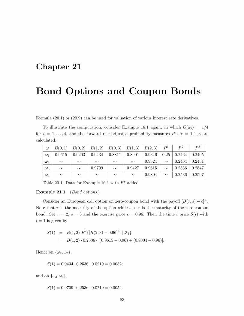
Chapter 21
Bond Options and Coupon Bonds
Formula (20.1) or (20.9) can be used for valuation of various interest rate derivatives.
To illustrate the computation, consider Example 16.1 again, in which Q(ωi) = 1/4for i = 1, . . . , 4, and the forward risk adjusted probability measures P τ , τ = 1, 2, 3 arecalculated.
ω B(0, 1) B(0, 2) B(1, 2) B(0, 3) B(1, 3) B(2, 3) P 1 P 2 P 3
ω1 0.9615 0.9203 0.9434 0.8811 0.8901 0.9346 0.25 0.2464 0.2405
ω2 ∼ ∼ ∼ ∼ ∼ 0.9524 ∼ 0.2464 0.2451
ω3 ∼ ∼ 0.9709 ∼ 0.9427 0.9615 ∼ 0.2536 0.2547
ω4 ∼ ∼ ∼ ∼ ∼ 0.9804 ∼ 0.2536 0.2597
Table 20.1: Data for Example 16.1 with P τ added
Example 21.1 (Bond options.)
Consider an European call option on zero-coupon bond with the payoff [B(τ, s) − c]+.Note that τ is the maturity of the option while s > τ is the maturity of the zero-couponbond. Set τ = 2, s = 3 and the exercise price c = 0.96. Then the time t price S(t) witht = 1 is given by
S(1) = B(1, 2) E2[B(2, 3)− 0.96]+ | F1= B(1, 2) · 0.2536 · [(0.9615− 0.96) + (0.9804− 0.96)].
Hence on ω1, ω2,
S(1) = 0.9434 · 0.2536 · 0.0219 = 0.0052;
and on ω3, ω4,
S(1) = 0.9709 · 0.2536 · 0.0219 = 0.0054.
83

If we use (20.1) instead, then
S(1) = EQ[B(2, 3)− 0.96]+B(1)/B(2) | F1.
Hence on ω1, ω2,
S(1) = 0.250.02191.06
= 0.0052;
and on ω3, ω4,
S(1) = 0.250.02191.03
= 0.0053.
Notice the discrepancy due to rounding errors. The two methods should yield the sameresult. In fact, Proposition 20.1 can be verified directly in this case by observing thatB(1, 2) = B(1) B(0, 2).
Other bond options can be priced in the same way.
Example 21.2 (Coupon bonds.)
A coupon bond is a contract entered at time t, say, such that a sequence of coupons ofc1, . . . , cN dollars will be paid at times t < t1 < · · · < tN ≤ T . By (20.1), the time t price ofthe coupon bond can be expressed as a linear combination of N zero-coupon bond prices:
S(t) =N∑
n=1
cnB(t, tn). (21.1)
Now use the data in Example 21.1 and consider an European put option with maturityτ = 2, exercise price c = 2.25, and based on the coupon bond with t1 = 2, t2 = 3, c1 = 1.1and c2 = 1.2. The time t = 1 price of the option is
S(1) = B(1, 2) E2[c− c1B(2, 2)− c2B(2, 3)]+ | F1.
Hence on ω1, ω2,
S(1) = 0.9434 · 0.2464 · (0.02848 + 0.00712) = 0.0083;
and on ω3, ω4,
S(1) = 0.9709 · 0.2464 · (0.02848 + 0.00712) = 0.0085.
If we use (20.1), then
S(1) = EQ[c− c1B(2, 2)− c2B(2, 3)]+B(1)/B(2) | F1.
84

Hence on ω1, ω2,
S(1) = 0.250.02848 + 0.00712
1.06= 0.0084;
and on ω3, ω4,
S(1) = 0.250.02848 + 0.00712
1.03= 0.0086.
85
Chapter 22
Swaps, Caps and Floors
A few more interest rate derivatives are studied in this lecture.
22.1 Swaps and swaptions
A swap is an agreement between a payer and a receiver. The payer pays a fixed rate κ to,and meanwhile receives a floating rate r from the receiver. Their payments are based ona common principal. The payment is made each period during a time interval. A swap issaid to be settled in arrears if one uses the spot rate r for the period just ended, or settledin advance if one uses the spot rate r for the period about to begin. With an ordinary swapthe initial floating rate payment is based on the spot rate at the time when the agreement ismade. With a forward start swap the initial floating rate payment is based on the spot ratesubsequent to the one when the agreement is made. We will mainly focus on payer forwardstart swap on principal one settled each period in arrears. Other cases can be handledsimilarly. The value of a swap is the expected present value of the net cash flow, i.e.
S(t) = EQ
τ ′∑s=τ
[r(s)− κ]B(t)B(s)
∣∣∣∣∣∣Ft
, t < τ ≤ τ ′ ≤ T. (22.1)
This formula can be simplified as follows:
S(t) = EQ
τ ′∑s=τ
[1
B(s− 1, s)− 1− κ
]B(t)B(s)
∣∣∣∣∣∣Ft
= EQ
τ ′∑s=τ
B(t)B(s)B(s− 1, s)
∣∣∣∣∣∣Ft
− (1 + κ) EQ
τ ′∑s=τ
B(t)B(s)
∣∣∣∣∣∣Ft
= EQ
τ ′∑s=τ
B(t)B(s− 1)
∣∣∣∣∣∣Ft
− (1 + κ)
τ ′∑s=τ
B(t, s)
86

=τ ′∑
s=τ
B(t, s− 1)− (1 + κ)τ ′∑
s=τ
B(t, s)
= B(t, τ − 1)− κτ ′−1∑s=τ
B(t, s)− (1 + κ) B(t, τ ′). (22.2)
The forward swap rate is the value of κ in (22.1) and (22.2) which makes the time t
value of the forward swap in [τ, τ ′] zero, denoted by
κ(t, τ, τ ′) =B(t, τ − 1)−B(t, τ ′)B(t, τ) + · · ·+ B(t, τ ′)
. (22.3)
A payer swaption is a European call option on the time τ −1 value of the correspondingpayer forward start swap, with exercise time τ − 1 and exercise price zero. For t < τ , thetime t value of the payer swaption is
Vp(t) = EQ
B(t)B(τ − 1)
EQ
τ ′∑s=τ
B(τ − 1)B(s)
(r(s)− κ)
∣∣∣∣∣∣Fτ−1
+∣∣∣∣∣∣Ft
.
A receiver swaption is defined similarly with its time t value
Vr(t) = EQ
B(t)B(τ − 1)
EQ
τ ′∑s=τ
B(τ − 1)B(s)
(κ− r(s))
∣∣∣∣∣∣Fτ−1
+∣∣∣∣∣∣Ft
.
Note that
Vp(t)− Vr(t) = EQ
B(t)B(τ − 1)
EQ
τ ′∑s=τ
B(τ − 1)B(s)
(r(s)− κ)
∣∣∣∣∣∣Fτ−1
∣∣∣∣∣∣Ft
= EQ
B(t)B(τ − 1)
τ ′∑s=τ
B(τ − 1)B(s)
(r(s)− κ)
∣∣∣∣∣∣Ft
= EQ
τ ′∑s=τ
B(t)B(s)
(r(s)− κ)
∣∣∣∣∣∣Ft
, (22.4)
which is the time t price of the forward start swap. Thus we have the following parity:
“payer swaption - receiver swaption = forward swap.”
By (22.2), another expression for the time t price of the payer swaption is
Vp(t) = EQ
B(t)B(τ − 1)
1− κ
τ ′−1∑s=τ
B(τ − 1, s)− (1 + κ) B(τ − 1, τ ′)
+ ∣∣∣∣∣∣Ft
,
which can be interpreted as this:
87

A payer swaption is same as a put option on a coupon bond, with exercise date τ − 1 andexercise price one. The coupon has face value one and coupon rate κ. Similarly, a receiverswaption can be interpreted as a call option on a coupon bond.
To have another interpretation, suppose for each s = τ, τ + 1, . . . , τ ′, there is a calloption with exercise time s and payoff [κ(τ − 1, τ, τ ′) − κ]+. The time τ − 1 value of thisportfolio consisting of a sequence of calls is given by
S(t) = EQ
B(t)B(τ − 1)
EQ
τ ′∑s=τ
B(τ − 1)B(s)
(κ(τ − 1, τ, τ ′) − κ)+∣∣∣∣∣∣Fτ−1
∣∣∣∣∣∣Ft
= EQ
B(t)B(τ − 1)
(κ(τ − 1, τ, τ ′) − κ)+ EQ
τ ′∑s=τ
B(τ − 1)B(s)
∣∣∣∣∣∣Fτ−1
∣∣∣∣∣∣Ft
= EQ
B(t)B(τ − 1)
(κ(τ − 1, τ, τ ′) − κ)+τ ′∑
s=τ
B(τ − 1, s)
∣∣∣∣∣∣Ft
= EQ
B(t)B(τ − 1)
1−B(τ − 1, τ ′)− κ
τ ′∑s=τ
B(τ − 1, s)
+∣∣∣∣∣∣Ft
, (22.5)
which is just the time t price of the payer swaption.
22.2 Caps and floors
A caplet is a European call option on the spot rate r(τ) at a specific time τ and with aspecified exercise price κ. Thus its time t price is
S(t) = EQ[r(τ)− κ]+B(t)/B(τ) | Ft = B(t, τ) Eτ[r(τ)− κ]+ | Ft.
A cap is a sequence of caplets which have a common exercise price. Like swaps, there areordinary and forward start caps, depending on whether the initial caplet corresponds to thecurrent spot rate. The time t price of a forward start cap in [τ, τ ′] settled in arrears is givenby
S(t) =τ ′∑
s=τ
EQ[r(s)− κ]+B(t)/B(s) | Ft, t < τ ≤ τ ′ ≤ T. (22.6)
A floorlet is defined in the same way as a caplet, but as a put option on the spot rate.A floor is a sequence of floorlets. The time t price of a forward start floor in [τ, τ ′] settledin arrears is given by
S(t) =τ ′∑
s=τ
EQ[κ− r(s)]+B(t)/B(s) | Ft, t < τ ≤ τ ′ ≤ T. (22.7)
88

It is obvious that the price of a cap minus the price of a floor is equal to the price of a swap.
Furthermore, a caption is a call or put option on a forward cap; while a floortion is acall or put option on a forward floor. These derivatives are examples of compound options.
89

Chapter 23
Implied Volatility
Financial models need to be fitted by real data in financial markets. This is called modelcalibration — a major task in empirical finance. An important special case is volatilityestimation. We start with some motivation then introduce a couple of approaches alongthis line.
23.1 Inverting the Black-Scholes formula
Recall the Black-Scholes formula (6.7) for a European call option price:
C = C(t, T ) = S(t) Φ(v1)− c e−r(T−t)Φ(v2),
where
v1 =log(S(t)/c) + (r + σ2/2) (T − t)
σ√
T − t
and
v2 = v1 − σ√
T − t =log(S(t)/c) + (r − σ2/2) (T − t)
σ√
T − t.
Notice that t, T, c and S(t) are clearly known to investors, but the parameters r and σ
need to be specified when applying formula (6.7). A more basic question is whether it isreasonable to assume that r and σ are constants. In fact, a lot of efforts have been madeto challenge and modified the basic assumptions for the Black-Scholes theory:
(i) constant parameters r and σ;
(ii) geometric Brownian motions as models for the underlying risky security S(t).
90

We skip the issue (ii) since this course is only limited to discrete-time models. For theissue (i), the case of stochastic spot rate r was studied in some previous lectures. Our focusnow is on modification of constant volatility σ.
A statistical interpretation of volatility σ dates back to the sequence of binomial treesin Lecture 6. For each positive integer n and fixed T > 0, we let the up and down factorsbe
un = ean (1 + rn)dn = e−an (1 + rn)
where an = σ√
δ and rn = rδ with two constant parameters r > 0, σ > 0, and δ = T/n.
For large n (or small δ), we can rewrite the two factors as
log un ≈ rδ + σ
√δ
log dn ≈ rδ − σ√
δ
where the LHS represent a one-step return with step size δ. Thus rδ is thought of as themean return, and σ
√δ the standard deviation.
This interpretation motivates a standard statistical method to estimate volatility σ,often referred to as historical volatility, in which the data consist of observations of returns,and the corresponding sample standard deviation is calculated as an estimate of volatilityσ. However, a different approach is used more often in daily practice of financial markets.
The basic strategy is to derive an estimate of σ by “inverting” a pricing formula suchas (6.7). Does the inversion work? In the case of (6.7), it turns out that for fixed t, T, c, r
and S(t), C is strictly increasing in σ. To verify this, notice that
dv1
dσ− dv2
dσ=√
T − t; (23.1)
and
S(t) φ(v1) = c φ(v2) e−r(T−t), (23.2)
where φ is the density function of N(0, 1). Therefore,
∂C
∂σ= S(t) φ(v1)
dv1
dσ− c e−r(T−t) φ(v2)
dv2
dσ
= S(t) φ(v1)(
dv1
dσ− dv2
dσ
)[by (23.2)]
= S(t) φ(v1)√
T − t [by (23.1)]
> 0. (23.3)
91

As the result of inverting (6.7),
σ = σ(C; t, T, c, r, S(t)),
is referred to as the implied volatility.
Note:
In general, a pricing formula need not be invertible. If it is invertible, then a corre-sponding implied volatility can be derived. Hence
an implied volatility depends on a particular pricing formula, while the historical volatil-ity aforementioned does not. In that sense, an implied volatility reflects the market vari-ability affected by certain specific securities, while the historical volatility is a measure ofoverall market variability or uncertainty.
23.2 Volatility smile
Options are referred to as in-the-money, at-the-money, or out-of-the-money. An in-the-money option is one that would lead to a positive cash flow to the holder if it were exercisedimmediately; similarly, an at-the-money option would lead to zero cash flow while an out-of-the-money option a negative cash flow. For a call option, the three cases correspond toS(τ) > c, S(τ) = c and S(τ) < c, respectively, at the expiry τ . Observed implied volatilitiesoften reveal a “smile”, which caricatures a nonlinear shape of an implied volatility plotagainst the exercise price c.
(See the attached figure.)
The volatility smile effect is a manifestation of violation of constant volatility assumptionin the Black-Scholes theory. Various factors in a financial market, such as exercise price c,affect the volatility. Even if the Black-Scholes model is slightly modified by allowing thevolatility to depend on the exercise price, i.e. σ = σ(c), it still cannot explain the volatilitysmile. To see this, apply the Implicit Function Theorem to the formula (6.7), we have
dσ
dc=−∂C
∂c∂C∂σ
.
By (23.3), dσdc and ∂C
∂c have opposite signs. By (23.2),
∂C
∂c= S(t) φ(v1)
dv1
dc− c e−r(T−t) φ(v2)
dv2
dc− e−r(T−t) Φ(v2)
= − e−r(T−t) Φ(v2)
< 0.
92

Hence dσdc > 0, i.e. σ is strictly increasing in c, which does not agree with the volatility
smile phenomenon.
A nonconstant volatility can be treated as a random variable, or a deterministic functionin time, or a stochastic process. The study of various stochastic volatility models has becomean active research area in which volatility itself is defined as a stochastic process.
Notes:
• Apart from volatility smile, another component of implied volatility is the term structureof volatility which describes the way at-the-money implied volatility varies with timeto expiration.
• Although in a stochastic volatility setting, volatility can be modelled in the same manneras stocks and bonds, volatility is neither an observable variable nor a tradable security.This brings up an important issue of hedging volatility risk — the risk associated withunanticipated changes in volatility. If there is a security, called volatility instrument,such that its price is perfectly correlated with volatility changes, then volatility riskcan be hedged out through this financial instrument. However, such a situation israre. In other words, a stochastic volatility model is an incomplete market in general.
93

Chapter 24
Implied Volatility Trees
The basic idea of implied volatility trees, introduced by Derman and Kani, is to build abinomial tree model for underlying securities with a given set of option prices as its input.It is designed so that (i) the option prices derived from the implied tree match the inputconsistently; (ii) certain parameters, such as volatility, can be inferred from the impliedtree; and (iii) more exotic options and other derivatives can be priced via the implied tree.
24.1 Construction of implied volatility trees via forward in-
duction
An implied volatility tree is a recombining binomial tree of security prices on the trianglelattice (t, k) : k = 0, 1, . . . , t; t = 0, 1, . . . , T (same as in Lecture 17 or Section 19.2). Thelattice could be renormalized by introducing a temporal increment δ = T/n and a spatialincrement
√δ as we did before in order to make a connection to some continuous-time
models, but we choose not doing it to keep the notation simple.
Using the forward induction, suppose the tree has been built up to time t. For a fixednode (t, k), we will show how to derive the security prices at (t + 1, k) and (t + 1, k + 1)based on the security price at (t, k) and some option prices at time t. In particular, assumethe knowledge of time t values of some European put options.
In general, each variable and parameter of interest can depend on time and state. Weadopt the following simplified notation:
• Up and down factors: u = u(t, k) from (t, k) to (t + 1, k + 1) and d = d(t, k) from (t, k)to (t + 1, k) respectively.
• Security prices: S = S(t, k), Su = S(t+1, k +1) = S u and Sd = S(t+1, k) = S d. Sincethe tree is recombining, Sd for (t, k) is also Su for (t, k − 1), and vice versa.
94

• Short rate in (t, t + 1]: r = r(t + 1) (recall that the short rate process is assumed to bepredictable).
• Risk neutral probability: q = q(t, k) = 1+r−du−d = (1+r)S−Sd
Su−Sd.
• The value of a European put at (t, k): V = Vput(t, k) with expiry t + 1 and strike pricec = S = S(t, k) (at-the-money put). This is equivalent to the knowledge of theEuropean call Vcall(t, k) with the same expiry t + 1 and same strike price c = S(t, k)because of the put-call parity.
Having built the tree up to time t, there are t+2 variables S(t+1, k), k = 0, 1, . . . , t+1to be specified. We establish t + 2 constraints with the following steps.
(i) Each node at time t has an at-the-money option pricing constraint
V = (1 + r)−1(1− q) (S − Sd), (24.1)
with the strike price c = S, where
1− q =Su − (1 + r)S
Su − Sd. (24.2)
This amounts to t + 1 constraints.
(ii) An additional constraint can be obtained by imposing the symmetry condition d = 1/u
at a particular node near the “center”, which is identified as (t, t/2) if t is even or(t, (t + 1)/2) if t is odd. From this central node (t, k), we compute the up factor as
u =V + S
(1 + r)−1S − V, (24.3)
and the down factor d = 1/u, then obtain Su and Sd. To verify (24.3), plugging (24.2)in (24.1) and reorganizing terms yields the equation
[(1 + r)−1S − V ] u− S [1 + (1 + r)−1] +S + V
u= 0,
which is equivalent to the quadratic equation
[(1 + r)−1S − V ] u2 − S [1 + (1 + r)−1] u + (S + V ) = 0, (24.4)
thus
u =S [1 + (1 + r)−1]± S[1− (1 + r)−1] + 2V
2 [(1 + r)−1S − V ]. (24.5)
We choose “+” since there is no guarantee that “−” will lead to a positive value of u.This will result in (24.3).
95

(iii) Having calculated Su = S(t+1, k+1) and Sd = S(t+1, k) from the central node (t, k),we compute security prices at nodes (t + 1, j) with j > k + 1 and j < k. Followingthe recombining property, Su for (t, k) is also Sd for (t, k + 1), and Sd for (t, k) is alsoSu for (t, k − 1). Therefore, using
Su =V Sd + S[(1 + r)−1Sd − S]
V + (1 + r)−1Sd − S, (24.6)
and
Sd =V Su + S[S − (1 + r)−1Su]
V + S − (1 + r)−1Su, (24.7)
security prices at all nodes at time t + 1 can be computed.
24.2 Specification of Vput via Arrow-Debreu securities
In the construction of an implied volatility tree, the option price V = Vput(t, k) correspond-ing to the strike price c = S(t, k) at each node (t, k) is needed as an input. First, note thatVput(t, j) = 0 for all j > k. Second, for j < k, we have
Vput(t, j) =S(t, k)
1 + r(t + 1)− S(t, j). (Why?)
Third, the data available in an option market is usually not Vput(t, k) at various nodes (t, k),but their averages. Let P (t, τ, c) denote the time t market price of a European put optionwith expiry τ and strike price c. Then
P (t, t + 1, S(t, k)) =k∑
j=0
pt,j Vput(t, j)
=k−1∑
j=0
pt,j
[S(t, k)
1 + r(t + 1)− S(t, j)
]+ pt,k Vput(t, k), (24.8)
which gives rise to
Vput(t, k) =P (t, t + 1, S(t, k))−∑k−1
j=0 pt,j
[S(t,k)
1+r(t+1) − S(t, j)]
pt,k, (24.9)
where pt,j is the probability (under the EMM Q) that the security attains the value S(t, j).
In this calculation, the known market price P (t, t + 1, S(t, k)) is represented as an av-erage of Vput(t, j) weighted by Arrow-Debreu probabilities pt,j, which can be calculated
96

iteratively by
pt+1,0 = [1− q(t, 0)] pt,0,
pt+1,t+1 = q(t, t) pt,t,
pt+1,k = q(t, k − 1) pt,k−1 + [1− q(t, k − 1)] pt,k, 1 ≤ k ≤ t. (24.10)
In particular, p0,0 = 1. Arrow-Debreu probabilities are related to Arrow-Debreu securities:the Arrow-Debreu security associated with each node (t, k) is a contingent claim at time t
which pays $1 if the state (t, k) is attained by the security and $0 otherwise. Although thesesecurities are not traded in the market, they can still be priced via the risk neutral valuationprinciple. Let (t′, k′) be a node with t′ < t, then at (t′, k′), the price of the Arrow-Debreusecurity associated with node (t, k) is the sum of probabilities attached to all paths thatlead from (t′, k′) to (t, k), multiplied by the discount factor [1 + r(t′ + 1)] · · · [1 + r(t)]−1.
24.3 How to deal with possible bad probabilities?
A possible complication in implementing the above procedure is that at a certain node(t, k), the resulting risk neutral probability q(t, k) may turn out to be a “bad probability”,i.e. 0 ≤ q ≤ 1 need not be satisfied, or equivalently, the inequalities Sd < S < Su may nothold. When that happens, we override the option price V that produces the bad node, andchoose the security prices that keep the local volatility
σ(t, k) =√
q(1− q) logSu
Sd
the same as that calculated at two preceding nodes. See [1] and [2] for more detaileddiscussions.
References [3] and [4] provide some alternative approaches to construct implied volatil-ity trees. [1] also contains results for implied trees concerning stocks with dividends andAmerican options.
References on “implied trees”:
[1] Chriss, N.A. (1997). Black-Scholes and Beyond. McGraw-Hill.
[2] Derman, E. and Kani, I. (1994). Riding on a smile. RISK 7(2), 32-39.
[3] Dupire, B. (1994). Pricing with a smile. RISK 7(1), 18-20.
[4] Rubinstein, M. (1994). Implied binomial trees. J. Finance 69(3), 771-818.
97

Problem Set 1
(1) In Example 4.1 (same as the example in Lecture 2 except for the interest rate r = 7%),
(1a) find an arbitrage opportunity;
(1b) show that the law of one price remains true.
(2) Construct a single period model (T = 1) for which the law of one price holds but thereexists an arbitrage opportunity.
(3) Do Exercise 4.3.
(4) Do Exercise 6.1.
(5) Recall the example in Lecture 2: u = 1.07, d = 0.92, r = 0.06, and the stock pricefollows the binomial tree in Figure 2.1.
(5a) Construct a put option tree (similar to Figure 2.2) with the exercise price c = $2.05.
(5b) For the chooser option (see Example 5.3) with the decision time T0 = 2, the expiryT = 3, and the exercise price c = $2.05, construct the replicating portfolio and represent itin a binomial tree similar to Figure 2.3.
(5c) Construct a binomial tree for the chooser option values under the conditions in (5b).
98

Problem Set 2
(1) Consider the binomial tree model: T = 3, u = 1.07, d = 0.92, r = 6% and S(0) = $2(see the example in Lecture 2). Suppose a constant dividend yield λ = 5% of the stockprice is issued at the ex-dividend date t = 2.
(1a) Calculate the value process of the American chooser option with the decision timeT0 = 1 and the exercise price c = $2.05.
(1b) Determine the optimal exercise strategy.
(2) Consider the binomial tree model with parameters T , u, d, r and p, whered < 1 + r < u. Assume the initial price S(0), the initial wealth w0 and the utility functionU(w) = log w, w > 0. Use dynamic programming to determine the optimal trading strategyand verify if your result agrees with the conclusion on Example 11.2 in Lecture 11.
(3) Consider the binomial tree model: T = 2, u = 1.07, d = 0.92, r = 4% and S(0) = $1;and assume the probability p = 0.6.
(3a) Solve the problem (P4) in Lecture 12 at t = 1 and with µ1 = 0.05.
(3b) At t = 1, calculate the risk premium EtR(t + 1) − r associated with a European calloption with the exercise price c = $1.
(3c) Do (3b) again using the CAPM (12.1), and compare your result here with what youobtained in (3b).
99

Problem Set 3
(1) Assume the stock price process starts with S(0) = 1 and follows a binomial tree withu = 1.08, d = 0.91. Moreover, the short rate process is the same as in Example 16.1.
(1a) Consider a forward contract and a futures contract on the stock, both start att = 0 and end at T = 3. Do they have the same value at t = 0? Why?
(1b) For a European call option and a European put option on the futures FU(1, 3),specify the exercise price c such that these two European options have the samevalue at t = 0.
(2) Consider the following numerical problem related to implied volatility. Use an iterativemethod, such as the Newton-Raphson method (or others if you prefer), to computethe implied volatility via the Black-Scholes formula for European call options, wherewe assume that the current stock price S(t) = $100, the strike price c = $100, thetime to expiration T − t = 2 (years), the annual interest rate r = 3% and the marketoption price C = $8.61. Briefly describe the algorithm(s) you use, with the parametersin your algorithm: initial values (e.g. you may try to start with an initial volatilityσ = 20%), number of steps, etc., report your results via tables or/and plots, and makecomments if necessary.
(3) Instead of an at-the-money option considered in (2), this problem involves a number ofdifferent strike prices given in the following table, in order to see whether the resultingimplied volatilities demonstrate a volatility smile. Calculate the implied volatilitiesand plot them against the strike prices.
Type of option Strike price Mean option price Implied volatility
call 90 4.75
call 95 1.375
call 100 0.5
put 90 0.5
put 95 2.875
Table 1: One day option prices. The current stock price S(t) = 93.625; the timeto expiration T − t = 22 (days); the annual interest rate r = 5.12%; a 360-dayyear assumed; the mean of the bid-ask prices for each option is used as the observedmarket option price. See Hull’s book Chapter 6 for more detailed discussion on optionsmarkets.
(4) Do Exercise 20.2.
(5) Consider several interest rate derivatives based on the model and data given in Example16.1.
100

(5a) For t = 0, τ = 1 and τ ′ = 2, find the value of κ such that Vp(t) = Vr(t), i.e.the payer and receiver swaptions have the same value at t = 0 (assuming theunderlying swap is ordinary and settled in advance).
(5b) For τ = 2 and τ ′ = 3, find the value of κ such that the cap and floor have thesame value at time t = 0 (both assumed to be ordinary and settled in arrears).
(5c) Consider a call caption and a put caption with the same expiration time τ = 2and the same exercise price c, based on the ordinary cap defined in (5b) [useyour result in (5b) as the value of κ]. Find the value of c such that the call andput captions have the same value at time t = 0.
101