lecture 5-simple linear regression model-estimator

ACE 562, University of Illinois at Urbana-Champaign 5-1

ACE 562 Fall 2005

Lecture 5: The Simple Linear Regression Model: Sampling Properties of the Least Squares Estimators

by Professor Scott H. Irwin

Required Reading: Griffiths, Hill and Judge. "Inference in the Simple Regression Model: Estimator Sampling Characteristics and Properties," Ch. 6 in Learning and Practicing Econometrics Optional Reading: Kennedy. “Appendix A: Sampling Distributions: The Foundation of Statistics,” in A Guide to Econometrics (Ag Library reserve)


Overview In the previous section, we specified a linear economic model that led to the following statistical model, known as the simple linear regression model

1 2t t ty x eβ β= + + We assumed that et and yt are independent and identically distributed normal random variables In compact form, the assumptions of the simple linear regression model are, SR1. 1 2 , 1,...,t t ty x e t Tβ β= + + = SR2. 1 2( ) 0 ( )t t tE e E y xβ β= ⇔ = + SR3. 2var( ) var( )t te y σ= = SR4. cov[ , ] cov[ , ] 0t s t se e y y t s= = ≠ SR5. The variable xt is not random and must take on at

least two different values SR6. 2 2

1 2~ (0, ) ~ ( , )t t te N y N xσ β β σ⇔ +


One sample of data was obtained consisting of observations on food expenditure and income for forty households

⇒We assumed that the sample data was generated by the previous statistical model

Given this sample of data, we developed the following rules (estimators) for estimating the intercept and slope parameters of the (true, but unknown) linear statistical model

1 1 12 2

2

1 1

T T T

t t t tt t t

T T

t tt t

T y x x yb

T x x

= = =

= =

−=

⎛ ⎞− ⎜ ⎟⎝ ⎠

∑ ∑ ∑

∑ ∑

1 2b y b x= −

Using the sample data and least squares estimators, we computed the following least squares estimates of the unknown intercept and slope for the statistical model

1 7.3832b = 2 0.2323b = At this point, the estimates are simply computed numbers that have no statistical properties!


We can never know how close these particular numbers are to the true values we are trying to estimate While we cannot know the accuracy of the least squares estimates, we can examine the properties of the estimator under repeated sampling

• As before, we imagine "hitting" the estimator with many hypothetical samples and examining its performance across the samples

Repeated sampling in the food expenditure example can be thought of as setting income levels to be the same across samples, so that we just randomly select new households for the given levels of income

• In effect, assume that we can perform a controlled experiment where the set of values for tx are fixed across repeated samples, but the values for ty vary randomly

Applying the least squares estimation rules to each new (hypothetical) sample leads to different 1 2and b b estimates Consequently, the least squares estimation rules b1 and b2 are random variables


Viewing b1 and b2 as random variables leads to the following important questions

• What are the means, variances, covariances, and forms of the sampling distributions for the random variables b1 and b2?

• Since the least squares estimators are only one way

of using the sample data to obtain estimates of the unknown parameters 1 2andβ β , how well do the least squares estimators compare to other estimators in repeated sampling?

If someone proposes an estimation rule for a particular statistical model, your next question should be: What are its sampling characteristics and how good is it?

---Griffiths, Hill and Judge, LPE, p.209


Means, Variances and Covariances of b1 and b2 The sampling distributions shown on the previous page can be developed theoretically We will concentrate on the derivation of two important properties of the sampling distribution of b2: mean and variance

• The derivations for the mean and variance of b1

and the covariance of b1 and b2 are similar, so there is no need to repeat the process

To develop the desired formulas for the mean and variance of b2, it is helpful to first derive a new version of the least squares formula for b2 We start by re-stating the original version,

1 1 12 2

2

1 1

T T T

t t t tt t t

T T

t tt t

T y x x yb

T x x

= = =

= =

−=

⎛ ⎞− ⎜ ⎟⎝ ⎠

∑ ∑ ∑

∑ ∑


The previous formula can be re-written as,

12

2

1

( )( )

( )

T

t tt

T

tt

x x y yb

x x

=

=

− −=

−

∑

∑

Simply multiplying out the right hand term of the numerator, we get,

1 1 12

2 2

1 1

( )( ) ( ) ( )

( ) ( )

T T T

t t t t tt t t

T T

t tt t

x x y y x x y x x yb

x x x x

= = =

= =

− − − − −= =

− −

∑ ∑ ∑

∑ ∑

or,

1 12

2

1

( ) ( )

( )

T T

t t tt t

T

tt

x x y y x xb

x x

= =

=

− − −=

−

∑ ∑

∑

Since, 1

( ) 0T

tt

x x=

− =∑ , this can be simplified to


12

2

1

( )

( )

T

t tt

T

tt

x x yb

x x

=

=

−=

−

∑

∑

Next,

21

T

t tt

b w y=

=∑

where,

2

1

( )

( )

tt T

tt

x xwx x

=

−=

−∑

Finally, substitute the original formula for the statistical model, 1 2t t ty x eβ β= + + , for yt,

2 1 21 1

( )T T

t t t t tt t

b w y w x eβ β= =

= = + +∑ ∑


or,

2 1 21 1 1

T T T

t t t t tt t t

b w w x w eβ β= = =

= + +∑ ∑ ∑

and,

2 21

T

t tt

b w eβ=

= +∑

since 1 1

and0 1T T

t t tt t

w w x= =

= =∑ ∑

This new formula for the least squares estimator is quite valuable in deriving properties of b2


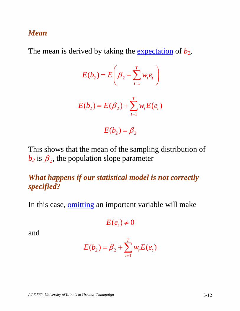
Mean The mean is derived by taking the expectation of b2,

2 21

( )T

t tt

E b E w eβ=

⎛ ⎞= +⎜ ⎟

⎝ ⎠∑

2 21

( ) ( ) ( )T

t tt

E b E w E eβ=

= +∑

2 2( )E b β=

This shows that the mean of the sampling distribution of b2 is 2β , the population slope parameter What happens if our statistical model is not correctly specified? In this case, omitting an important variable will make

( ) 0tE e ≠ and

2 21

( ) ( )T

t tt

E b w E eβ=

= +∑


If 2β is positive and the omitted variable tends to increase the size of positive errors, then

2 2( )E b β> If 2β is positive and the omitted variable tends to increase the size of negative errors, then

2 2( )E b β< Discussion highlights the importance of using economic theory to correctly specify the statistical model • Specification questions dominate applied

econometric work

• We will discuss this issue extensively next semester


Variance The variance of b2 in repeated samples is

2 22 2 2 2 2var( ) [ ( )] [ ]b E b E b E b β= − = −

Variance measures the precision of 2b in the sense that it tells us how much the estimates produced by 2b vary from sample-to-sample • The lower the variance of an estimator, the greater

the sampling precision

• The greater the variance of an estimator, the lower the sampling precision

Key point: An estimator is considered more precise than another estimator if its sampling variance is less than that of another estimator

Econometricians place a high priority on developing precise estimators


We can derive the variance of b2 as follows,

2 21 1

var( ) var varT T

t t t tt t

b w e w eβ= =

⎛ ⎞ ⎛ ⎞= + =⎜ ⎟ ⎜ ⎟

⎝ ⎠ ⎝ ⎠∑ ∑

2

21 1 1

var( ) var( ) cov( , )T T T

t t t s t st t s

b w e w w e e t s= = =

= + ≠∑ ∑∑

2

21

var( ) var( )T

t tt

b w e=

= ∑

2 2 2 2

21 1

var( )T T

t tt t

b w wσ σ= =

= =∑ ∑

and,

22

2

1

1var( )( )

T

tt

bx x

σ

=

⎡ ⎤⎢ ⎥

= ⎢ ⎥⎢ ⎥−⎢ ⎥⎣ ⎦∑

where 2

21

1

1

( )

T

t Tt

tt

wx x=

=

=−

∑∑


The standard deviation of 2b is found in the usual manner

2 22

1

1( ) var( )( )

T

tt

se b bx x

σ

=

⎡ ⎤⎢ ⎥⎢ ⎥= =⎢ ⎥

−⎢ ⎥⎢ ⎥⎣ ⎦∑

Notice that the term "standard error" (se) is normally used in place of standard deviation of the sampling distribution To see why, define the error that arises in estimating the true slope parameter as 2 2f b β= − Applying our rules for the mean and variance of the transformation of a random variable we find that

2( ) 0 var( ) var( )andE f f b= = Since the expected estimation error is zero, we can say that the typical error (without regard to sign) is given by the standard deviation of f, which equals the standard deviation of 2b If we replace "typical" with "standard" we can say that

2( )se b measures the standard estimation error for 2b , or in abbreviated form, standard error


Form Now that we have derived the mean and variance of the sampling distribution of b2, we can turn our attention to the form of the sampling distribution Earlier, we noted that

21

T

t tt

b w y=

=∑

where,

2

1

( )

( )

tt T

tt

x xwx x

=

−=

−∑

Writing the formula in the above format shows that the least squares rule b2 is a linear function of the yt • The yt are normally distributed (by assumption)

• Any linear function of normally distributed random

variables is itself normally distributed


Thus, b2 is normally distributed in repeated sampling

22 2

2

1

1~ ,( )

T

tt

b Nx x

β σ

=

⎛ ⎞⎡ ⎤⎜ ⎟⎢ ⎥⎜ ⎟⎢ ⎥⎜ ⎟⎢ ⎥−⎜ ⎟⎢ ⎥⎣ ⎦⎝ ⎠

∑

We will simply state the mean and variance results for b1,

1 1( )E b β=

2

2 11

2

1

var( )( )

T

tt

T

tt

xb

T x xσ =

=

⎡ ⎤⎢ ⎥

= ⎢ ⎥⎢ ⎥−⎢ ⎥⎣ ⎦

∑

∑

Using a similar argument as we did for b2, it can be shown that

2

2 11 1

2

1

~ ,( )

T

tt

T

tt

xb N

T x xβ σ =

=

⎛ ⎞⎡ ⎤⎜ ⎟⎢ ⎥⎜ ⎟⎢ ⎥⎜ ⎟⎢ ⎥−⎜ ⎟⎢ ⎥⎣ ⎦⎝ ⎠

∑

∑


Covariance Finally, the covariance between random variables b1 and b2 in repeated sampling is,

21 2

2

1

cov( , )( )

T

tt

xb bx x

σ

=

⎡ ⎤⎢ ⎥−

= ⎢ ⎥⎢ ⎥−⎢ ⎥⎣ ⎦∑


Probability Calculations Using Sampling Distributions While it is fun (!) to simply derive sampling distributions, their real usefulness is found in making probability statements about our estimates Let's suppose that the true regression model is

8 0.25t t ty x e= + + and all of the standard assumptions hold for the error term and 2 50σ = Now assume that we are "given" a set of T = 25 values for the independent variable tx and

2

1

( ) 15,000T

tt

x x=

− =∑

We now have all the information to derive the sampling distribution of b2 The expected value of b2 is given in this example as

2 2( ) 0.25E b β= =


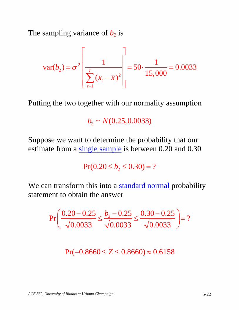
The sampling variance of b2 is

22

2

1

1 1var( ) 50 0.003315,000( )

T

tt

bx x

σ

=

⎡ ⎤⎢ ⎥

= = ⋅ =⎢ ⎥⎢ ⎥−⎢ ⎥⎣ ⎦∑

Putting the two together with our normality assumption

2 ~ (0.25,0.0033)b N Suppose we want to determine the probability that our estimate from a single sample is between 0.20 and 0.30

2Pr(0.20 0.30) ?b≤ ≤ = We can transform this into a standard normal probability statement to obtain the answer

20.20 0.25 0.25 0.30 0.25Pr ?0.0033 0.0033 0.0033

b− − −⎛ ⎞≤ ≤ =⎜ ⎟⎝ ⎠

Pr( 0.8660 0.8660) 0.6158Z− ≤ ≤ ≈


Factors That Affect the Variances and Covariance of the Sampling Distributions of b1 and b2

2

2 11

2

1

var( )( )

T

tt

T

tt

xb

T x xσ =

=

⎡ ⎤⎢ ⎥

= ⎢ ⎥⎢ ⎥−⎢ ⎥⎣ ⎦

∑

∑ 2

22

1

1var( )( )

T

tt

bx x

σ

=

⎡ ⎤⎢ ⎥

= ⎢ ⎥⎢ ⎥−⎢ ⎥⎣ ⎦∑

21 2

2

1

cov( , )( )

T

tt

xb bx x

σ

=

⎡ ⎤⎢ ⎥−

= ⎢ ⎥⎢ ⎥−⎢ ⎥⎣ ⎦∑

Important observations: 1. The variance of the error term ( 2σ ) appears in each

formula • The larger the variance, 2σ , the greater the

uncertainty about where the values of yt will fall relative to the population mean, ( )tE y

⇒Sample information available to estimate 1β and

2β is less precise the larger is 2σ


2. The sum of squares for xt 2

1( )

T

tt

x x=

⎛ ⎞−⎜ ⎟

⎝ ⎠∑ appears in the

denominator of each formula • Sum of squares for xt measures the spread, or

variation, of xt • The larger the variation in xt, the smaller are the

variances and covariance of b1 and b2 ⇒The more information we have about xt, the more precisely can we estimate 1β and 2β

3. The larger the sample size T, the smaller the variances

and covariance of b1 and b2 • As T increases, the sum of squares for increases

unambiguously • Effect is clear for 2var( )b and 1 2cov( , )b b • Same impact on 1var( )b because T and variation in xt

appear in denominator

⇒The more information we have about xt, the more precisely can we estimate 1β and 2β


xtxt xt

yt yt

Which data sample would you rather use to estimate the linear relationship between x and y?

xx

yy


4. The term 2

1

T

tt

x=∑ appears in the numerator of the formula

for 1var( )b

• 2

1

T

tt

x=∑ measures the distance of the data on xt from the

origin

⇒The more distant from zero are the data on xt, the independent variable, the more difficult it is to accurately estimate the intercept 1β

5. x appears in the numerator of 1 2cov( , )b b • Covariance has the opposite sign as x • Covariance increases in magnitude the larger is x

An understanding of the previous five points is of great value when interpreting regression results in applied research


yt

y

x xt

yt

y

x xt

Which data sample would you rather use to estimate the intercept in the linear relationship between x and y?


xtxt xt

yt yt

Demonstration of negative covariance between slope and intercept estimates when mean of x is positive

xx

yy


Summary of Key Factors Affecting Precision of Least Squares Estimators In the following table, characteristics of the sample data are categorized in terms of impact on precision Sample Characteristic

More Precision

Less Precision

High Variance of yt Low Variance of yt High Variation in xt Low Variation in xt Large T Small T Small Distance from Origin and xt Large Distance from Origin and xt


Sampling Properties of the Least Squares Estimators Since there are a number of different rules for obtaining estimates of 1β and 2β , how can we be assured that b1 and b2 are the "best" rules? Previously, we developed four main criteria for "good" estimators • Computational cost: Estimator is a linear function of

sample data

• Unbiasedness: In repeated sampling, the estimator generates estimates that on average equal the population parameter

• Efficiency: Of all possible unbiased estimators, there

is no other estimator that has a smaller variance

• Consistency: As the sample size increases the probability mass of the of estimator "collapses" on the population parameter

We will examine the least squares estimator b2 to see if it meets these four criteria Similar results hold for b1


Computational Cost Earlier, we noted that,

21

T

t tt

b w y=

=∑

where,

2

1

( )

( )

tt T

tt

x xwx x

=

−=

−∑

Writing the formula in the above format shows that the least squares rule b2 is a linear function of the yt Unbiasedness We want to know whether the expected value of b2 is in fact equal to 2β Earlier, we showed that the mean is derived by taking the expectation of the following version of the formula for b2,

2 21

( )T

t tt

E b E w eβ=

⎛ ⎞= +⎜ ⎟

⎝ ⎠∑


2 21

( ) ( ) ( )T

t tt

E b E w E eβ=

= +∑

2 2( )E b β=

Shows that the least squares estimator b2 is unbiased Efficiency For a given sample size T, we want to know whether the sampling variance of b2 is smaller than any other unbiased, linear estimator

• Desire an estimator that gives us the highest probability of obtaining an estimate close to the true parameter value

In other words, is there a different estimator that produces a sampling variance smaller than the following formula,

22

2

1

1var( )( )

T

tt

bx x

σ

=

⎡ ⎤⎢ ⎥

= ⎢ ⎥⎢ ⎥−⎢ ⎥⎣ ⎦∑


For all unbiased linear estimators, var(b2) is the smallest sampling variance possible

• Proof is found on pp. 78-79 of Hill et. al,

Undergraduate Econometrics and many other texts Consistency We want to show that as the sample size increases, the probability mass of the of estimator "collapses" on the population parameter This can be demonstrated informally by noting the formula for the sampling variance of b2,

22

2

1

1var( )( )

T

tt

bx x

σ

=

⎡ ⎤⎢ ⎥

= ⎢ ⎥⎢ ⎥−⎢ ⎥⎣ ⎦∑

and that

22

2

1

1lim var( ) 0( )

T

tt

bT x x

σ

=

⎡ ⎤⎢ ⎥

= =⎢ ⎥⎢ ⎥→∞ −⎢ ⎥⎣ ⎦∑


Summary of Sampling Properties Discussion The least squares estimators b1 and b2 of the population parameters 1β and 2β are,

• Linear

• Unbiased

• Efficient

• Consistent

The first three properties are sufficient to prove that b1 and b2 are the best linear unbiased estimators (BLUE) of

1β and 2β

• In this context "best" implies minimum variance sampling distribution

• Known as the Gauss-Markov Theorem


Key Points: • The estimators b1 and b2 are “best” when compared

to similar estimators, those that are linear and unbiased. The Gauss-Markov Theorem does not say that b1 and b2 are the best of all possible estimators.

• The estimators b1 and b2 are best within their class

because they have the minimum variance. • In order for the Gauss-Markov Theorem to hold, the

assumptions (SR1-SR5) must be true. If any of the assumptions 1-5 are not true, then b1 and b2 are not the best linear unbiased estimators of 1β and 2β .

• The Gauss-Markov Theorem does not depend on the

assumption of normality. • In the simple linear regression model, if we want to

use a linear and unbiased estimator, then we have to do no more searching.

• The Gauss-Markov theorem applies to the least

squares estimators. It does not apply to the least squares estimates from a single sample.


Estimating the Variance of the Error Term Recall that et and yt were assumed to be iid with the following distributions,

2 21 2~ (0, ) )and ~ ( ,t t te N y N xσ β β σ+

Unless 2σ is known, which is highly unlikely, it will have to be estimated as well Again, we cannot use the least squares principle, as 2σ does not appear in the sum of squares function,

2 21 2 1 2

1 1

( , ) ( )T T

t t tt t

S e y xβ β β β= =

= = − −∑ ∑

Instead, we apply a "heuristic" procedure based on the definition of 2σ


The original definition of 2σ in the statistical model is,

2 2var( ) var( ) [ ]t t ty e E eσ= = = In other words, the variance is the expected value of the squared errors Given this definition, it would be natural to estimate 2σ as the average of the squared errors In order to do this, we must first obtain estimates of the population errors using our sample data as

1 2t̂ t te y b b x= − − We can then develop our sample estimator of 2σ as,

22 2 2

2 11 2

ˆˆ ˆ ˆ...ˆ

2 2

T

ttT

ee e e

T Tσ =+ + +

= =− −

∑

Notice the squared sample errors are averaged by dividing by T-2 not T (or T-1)

• Accounts for the fact that 2 regression parameters 1 2( , )β β have to be estimated


Many regression packages report something called the "standard error of the regression" This is simply the square root of the estimated variance of the error term,

22 2 2

2 11 2

ˆˆ ˆ ˆ...ˆ ˆ

2 2

T

ttT

ee e e

T Tσ σ =+ + += = =

− −

∑

Warning: Do not confuse the standard error of the regression with the standard error of the sampling distribution of the least squares estimators 1 2an d b b


Sampling Properties of Variance Estimator The rule derived for estimating the population variance of the error term ( 2σ ) is,

2

2 1

ˆˆ

2

T

tt

e

Tσ ==

−

∑

Just as was the case with b1 and b2, we are interested in the sampling properties of 2σ̂ The same four criteria are applied when asking whether

2σ̂ is a "good" estimation rule

• Computational cost, unbiasedness, efficiency, consistency

It is obvious that 2σ̂ is not a linear estimator It can be shown that 2σ̂ is unbiased, efficient, and consistent

• Best unbiased estimator (BUE)

• Proof can be found in advanced econometrics books


The next issue is the form of the sampling distribution of the variance estimator 2σ̂ To derive the sampling distribution, first note that the population random errors are distributed as,

2~ (0, ) 1,...,te N t Tσ = Consequently,

~ (0,1) 1,...,te N t Tσ

=

and,

2

1~ 1,...,te t Tχσ⎛ ⎞ =⎜ ⎟⎝ ⎠

If we sum over the T transformed random errors,

2

1~

Tt

Ti

e χσ=

⎛ ⎞⎜ ⎟⎝ ⎠

∑


Based on the previous result, we can generate the sampling distribution of 2σ̂ ,

22

2ˆ ~2 TT

σσ χ −−

Note that the sampling distribution of 2σ̂ is proportional to a chi-square with T-2 degrees of freedom


Estimators of the Variances and Covariance of b1 and b2 Recall that the variances and covariance of the sampling distributions of b1 and b2 were functions of the unknown parameter 2σ We can generate estimators of the variances and covariances of b1 and b2 by simply replacing 2σ with 2σ̂ in the earlier formulas,

2

2 11

2

1

ˆ ˆvar( )( )

T

tt

T

tt

xb

T x xσ =

=

⎡ ⎤⎢ ⎥

= ⎢ ⎥⎢ ⎥−⎢ ⎥⎣ ⎦

∑

∑

22

2

1

1ˆ ˆvar( )( )

T

tt

bx x

σ

=

⎡ ⎤⎢ ⎥

= ⎢ ⎥⎢ ⎥−⎢ ⎥⎣ ⎦∑

21 2

2

1

ˆ ˆcov( , )( )

T

tt

xb bx x

σ

=

⎡ ⎤⎢ ⎥−

= ⎢ ⎥⎢ ⎥−⎢ ⎥⎣ ⎦∑


Likewise, the estimators for the standard errors of b1 and b2 are,

2

2 11 1

2

1

ˆˆ ˆ( ) var( )( )

T

tt

T

tt

xse b b

T x xσ =

=

⎡ ⎤⎢ ⎥

= = ⎢ ⎥⎢ ⎥−⎢ ⎥⎣ ⎦

∑

∑

22 2

2

1

1ˆˆ ˆ( ) var( )( )

T

tt

se b bx x

σ

=

⎡ ⎤⎢ ⎥

= = ⎢ ⎥⎢ ⎥−⎢ ⎥⎣ ⎦∑

This material is tricky:

• We developed estimators of the variances, covariance and standard errors of the least squares estimators of b1 and b2 !!

• While we will not consider the extra complexity,

the estimators of the variances, covariance and standard errors are themselves random variables whose values vary in repeated sampling


Sample Estimates of the Variances and Covariance of b1 and b2

We can now use our sample data on food expenditure and income to generate estimates of the variances and covariance of b1 and b2 First, estimate the variance of the error term,

2

2 1

ˆ1780.4ˆ 46.853

2 38

T

tt

e

Tσ == = =

−

∑

and the standard error of the regression,

2ˆ ˆ 46.853 6.845σ σ= = = Next, estimate the variances, standard errors, and covariance of b1 and b2,

2

2 11

2

1

ˆ ˆvar( ) 46.853(0.3429) 16.0669( )

T

tt

T

tt

xb

T x xσ =

=

⎡ ⎤⎢ ⎥

= = =⎢ ⎥⎢ ⎥−⎢ ⎥⎣ ⎦

∑

∑


1 1ˆˆ ( ) var( ) 16.0669 4.0083se b b= = =

22

2

1

1ˆ ˆvar( ) 46.853(0.0000653) 0.0031( )

T

tt

bx x

σ

=

⎡ ⎤⎢ ⎥

= = =⎢ ⎥⎢ ⎥−⎢ ⎥⎣ ⎦∑

2 2ˆˆ ( ) var( ) 0.0031 0.0557se b b= = =

21 2

2

1

ˆ ˆcov( , ) 46.853( 0.00455) 0.2134( )

T

tt

xb bx x

σ

=

⎡ ⎤⎢ ⎥−

= = − = −⎢ ⎥⎢ ⎥−⎢ ⎥⎣ ⎦∑


Sample Regression Output from Excel

SUMMARY OUTPUT

Regression StatisticsMultiple R 0.563096017R Square 0.317077125Adjusted R Square 0.29910547Standard Error 6.844922384Observations 40

ANOVAdf SS MS F Significance F

Regression 1 826.6352172 826.6352 17.64318 0.000155136Residual 38 1780.412573 46.85296Total 39 2607.04779

Coefficients Standard Error t Stat P-value Lower 95% Upper 95%Intercept 7.383217543 4.008356335 1.841956 0.073296 -0.731275911 15.497711X Variable 1 0.23225333 0.055293429 4.200378 0.000155 0.120317631 0.34418903


Summary of Estimates for Food Expenditure Data

1 7.3832b = 2 0.2323b = 2ˆ 46.853σ =

1ˆvar( ) 16.0669b = 2ˆvar( ) 0.0031b =

1 2ˆcov( , ) 0.2134b b = − Based on this information and the assumption that the statistical model is correctly specified, we can estimate the distributions of et and yt as,

~ (0, 46.853) ~ (7.382 0.2323 , 46.853)t t te N y N x+ We also can estimate the sampling distributions of b1 and b2 as,

1 2~ (7.382,16.0669) ~ (0.2323, 0.0031)b N b N


Interpretation Guidelines Regression standard error

2ˆ ˆ 46.853 6.845σ σ= = =

We say, “The typical error of the regression model, without regard to sign, is estimated to be $6.845/week.”

Standard error of parameter estimates

1 1ˆˆ ( ) var( ) 16.0669 4.0083se b b= = =

We say, “The typical error in estimating 1β , without regard to sign, is estimated to be 4.0083.”

2 2ˆˆ ( ) var( ) 0.0031 0.0557se b b= = =

We say, “The typical error in estimating 2β , without regard to sign, is estimated to be 0.0557.”

lecture 5-simple linear regression model-estimator

Documents