Lecture 4 #-1

Scheduling:Buffer Management

Lecture 4 #-2

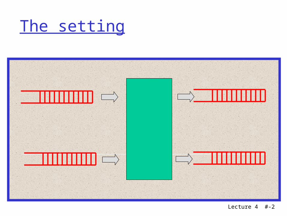
The setting

Lecture 4 #-3

Buffer Scheduling Who to send next? What happens when buffer is full? Who to discard?

Lecture 4 #-4

Requirements of scheduling

An ideal scheduling discipline is easy to implement is fair and protective provides performance bounds

Each scheduling discipline makes a different trade-off among these requirements

Lecture 4 #-5

Ease of implementation

Scheduling discipline has to make a decision once every few microseconds!

Should be implementable in a few instructions or hardware for hardware: critical constraint is VLSI space Complexity of enqueue + dequeue processes

Work per packet should scale less than linearly with number of active connections

Lecture 4 #-6

Fairness

Intuitivelyeach connection should get no more than its

demandthe excess, if any, is equally shared

But it also provides protectiontraffic hogs cannot overrun othersautomatically isolates heavy users

Lecture 4 #-7

Max-min Fairness: Single Buffer

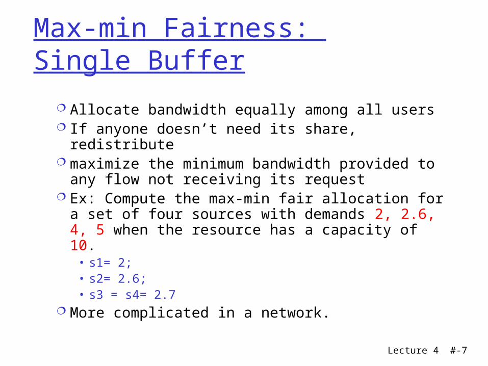
Allocate bandwidth equally among all users If anyone doesn’t need its share, redistribute maximize the minimum bandwidth provided

to any flow not receiving its request Ex: Compute the max-min fair allocation for a

set of four sources with demands 2, 2.6, 4, 5 when the resource has a capacity of 10.

• s1= 2; • s2= 2.6; • s3 = s4= 2.7

More complicated in a network.

Lecture 4 #-8

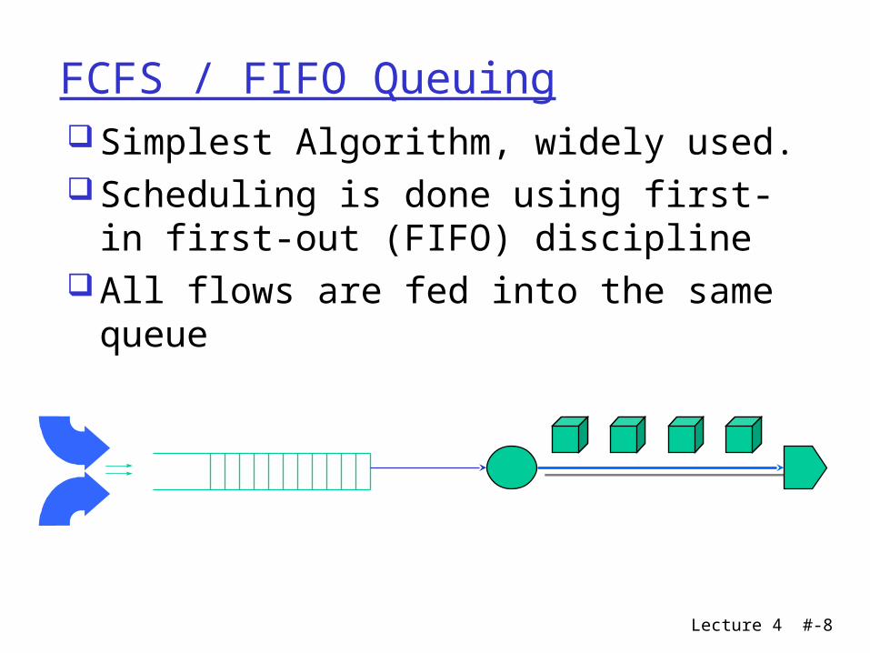
FCFS / FIFO QueuingSimplest Algorithm, widely used.Scheduling is done using first-in first-

out (FIFO) disciplineAll flows are fed into the same queue

Lecture 4 #-9

FIFO Queuing (cont’d)

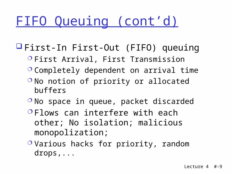
First-In First-Out (FIFO) queuing First Arrival, First Transmission Completely dependent on arrival time No notion of priority or allocated buffers No space in queue, packet discarded Flows can interfere with each other; No

isolation; malicious monopolization; Various hacks for priority, random drops,...

Lecture 4 #-10

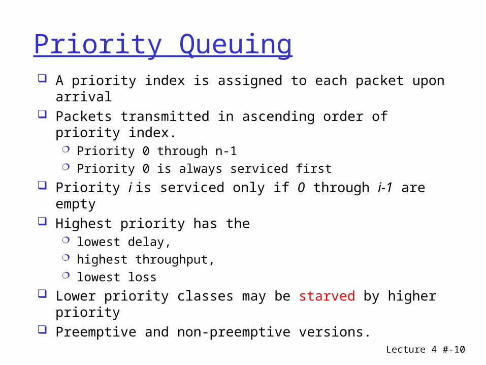
Priority Queuing A priority index is assigned to each packet upon arrival Packets transmitted in ascending order of priority index.

Priority 0 through n-1 Priority 0 is always serviced first

Priority i is serviced only if 0 through i-1 are empty Highest priority has the

lowest delay, highest throughput, lowest loss

Lower priority classes may be starved by higher priority Preemptive and non-preemptive versions.

Lecture 4 #-11

Priority Queuing

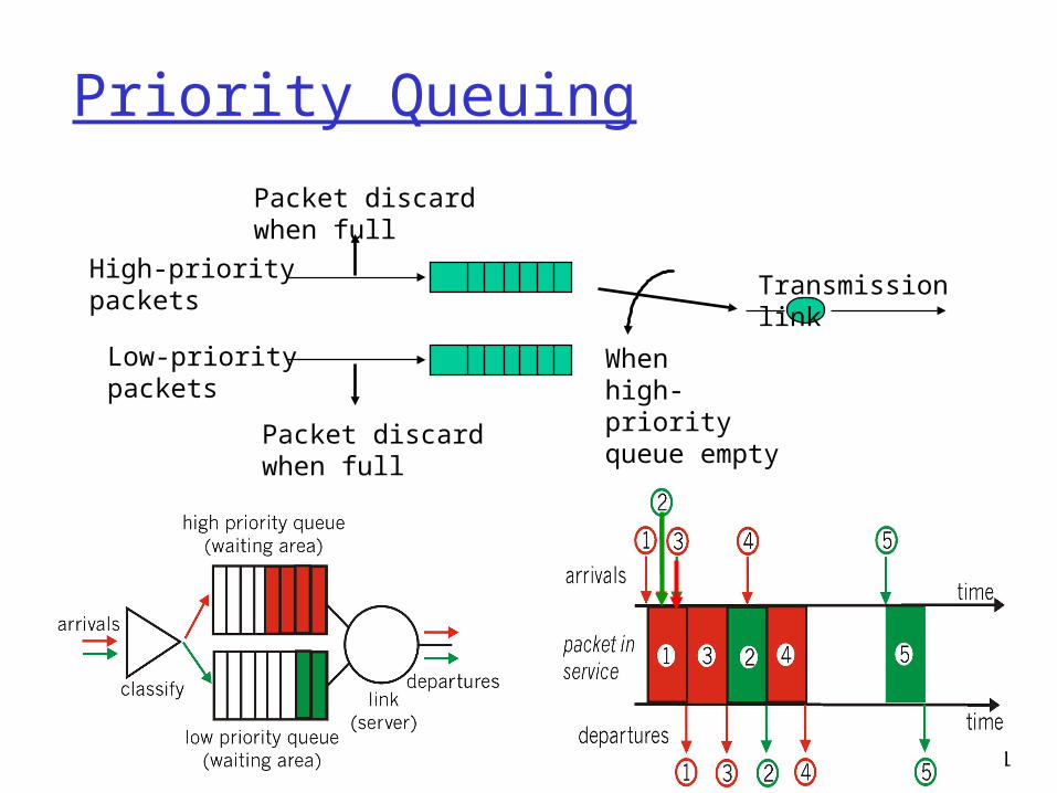
Transmission link

Packet discardwhen full

High-prioritypackets

Low-prioritypackets

Packet discardwhen full

When high-priorityqueue empty

Lecture 4 #-12

Round Robin: Architecture

Flow 1

Flow 3

Flow 2

Transmission link

Round robin

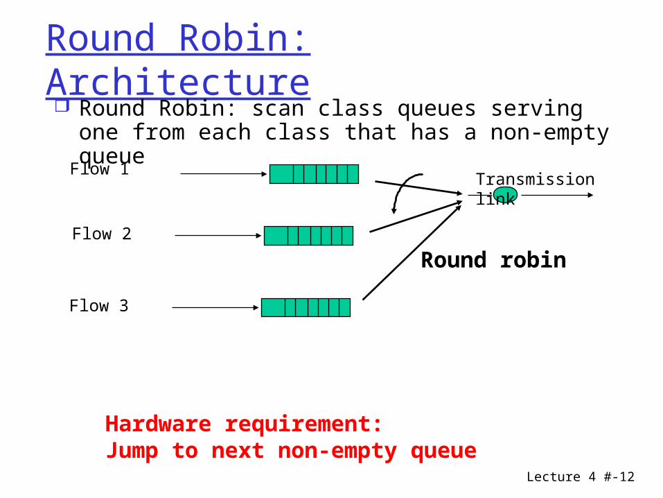
Hardware requirement: Jump to next non-empty queue

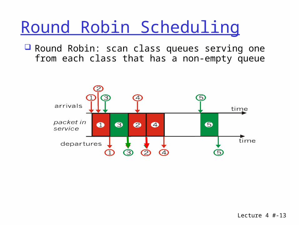
Round Robin: scan class queues serving one from each class that has a non-empty queue

Lecture 4 #-13

Round Robin Scheduling Round Robin: scan class queues serving one

from each class that has a non-empty queue

Lecture 4 #-14

Round Robin (cont’d) Characteristics:

Classify incoming traffic into flows (source-destination pairs)

Round-robin among flows Problems:

Ignores packet length (GPS, Fair queuing) Inflexible allocation of weights (WRR,WFQ)

Benefits: protection against heavy users (why?)

Lecture 4 #-15

Weighted Round-Robin Weighted round-robin

Different weight wi (per flow)

Flow j can sends wj packets in a period.

Period of length wj

Disadvantage Variable packet size. Fair only over time scales longer than a period time.

• If a connection has a small weight, or the number of connections is large, this may lead to long periods of unfairness.

Lecture 4 #-16

DRR algorithm Choose a quantum of bits to serve from each

connection in order. For each HOL (Head of Line) packet,

if its size is <= (quantum + credit) send and save excess,

otherwise save entire quantum. If no packet to send, reset counter (to remain fair)

Each connection has a deficit counter (to store credits) with initial value zero.

Easier implementation than other fair policies WFQ

Lecture 4 #-17

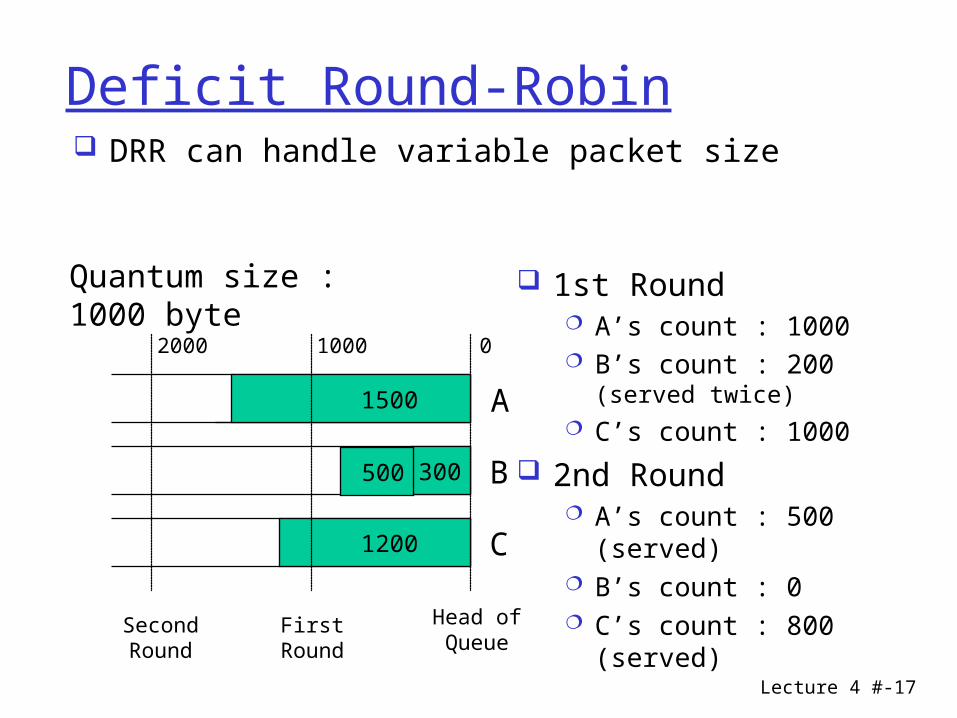
Deficit Round-Robin DRR can handle variable packet size

1500

300

1200

2000 1000

SecondRound

FirstRound

Head ofQueue

A

B

C

0

Quantum size : 1000 byte

1st Round A’s count : 1000 B’s count : 200 (served

twice) C’s count : 1000

2nd Round A’s count : 500 (served) B’s count : 0 C’s count : 800 (served)

500

Lecture 4 #-18

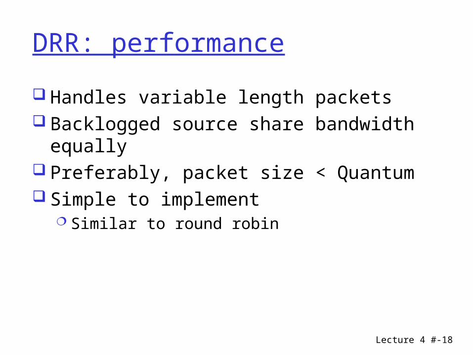
DRR: performance

Handles variable length packets Backlogged source share bandwidth

equally Preferably, packet size < Quantum Simple to implement

Similar to round robin

Lecture 4 #-19

Generalized Processor Sharing

Lecture 4 #-20

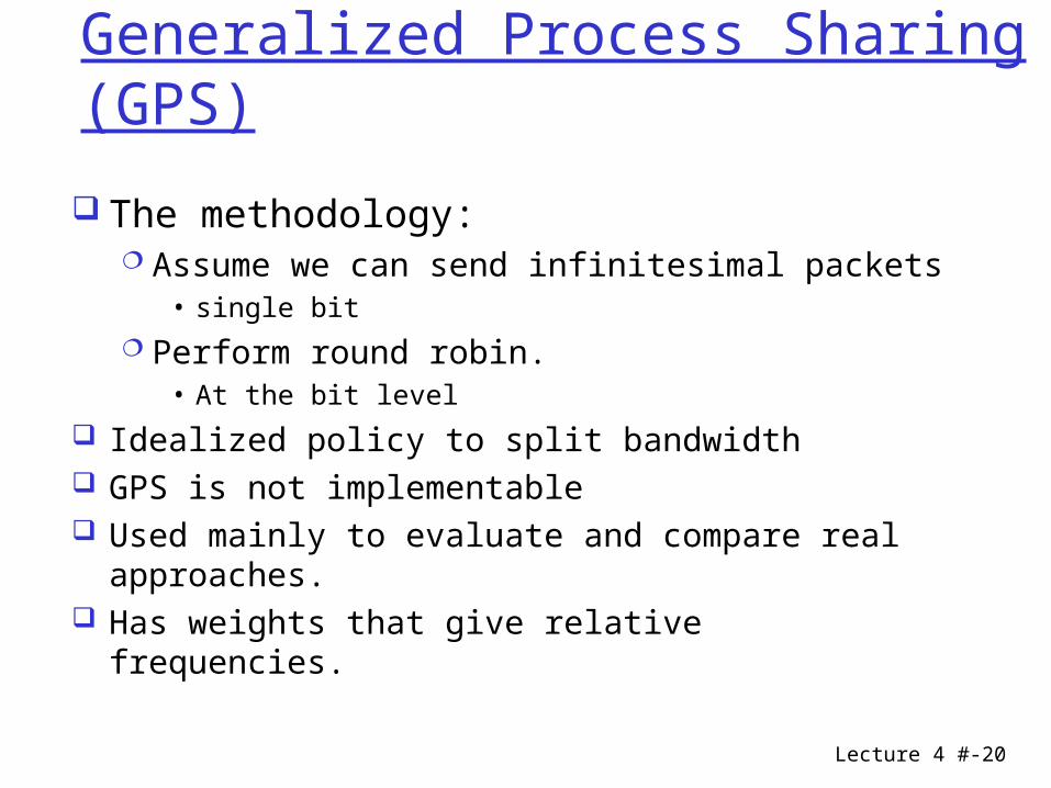
Generalized Process Sharing (GPS)

The methodology: Assume we can send infinitesimal packets

• single bit Perform round robin.

• At the bit level

Idealized policy to split bandwidth GPS is not implementable Used mainly to evaluate and compare real

approaches. Has weights that give relative frequencies.

Lecture 4 #-21

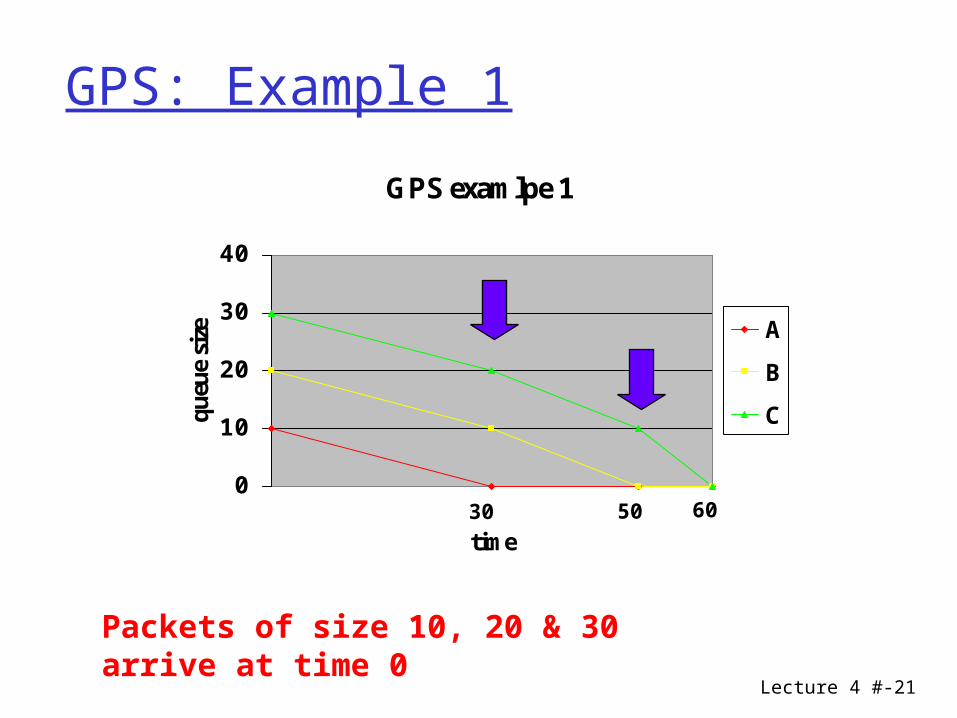
GPS: Example 1

GPS examlpe 1

0

10

20

30

40

time

queu

e si

ze A

B

C

50 6030

Packets of size 10, 20 & 30 arrive at time 0

Lecture 4 #-22

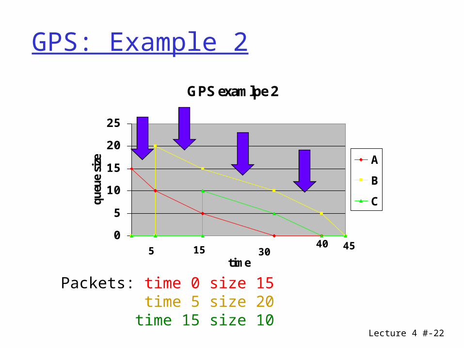
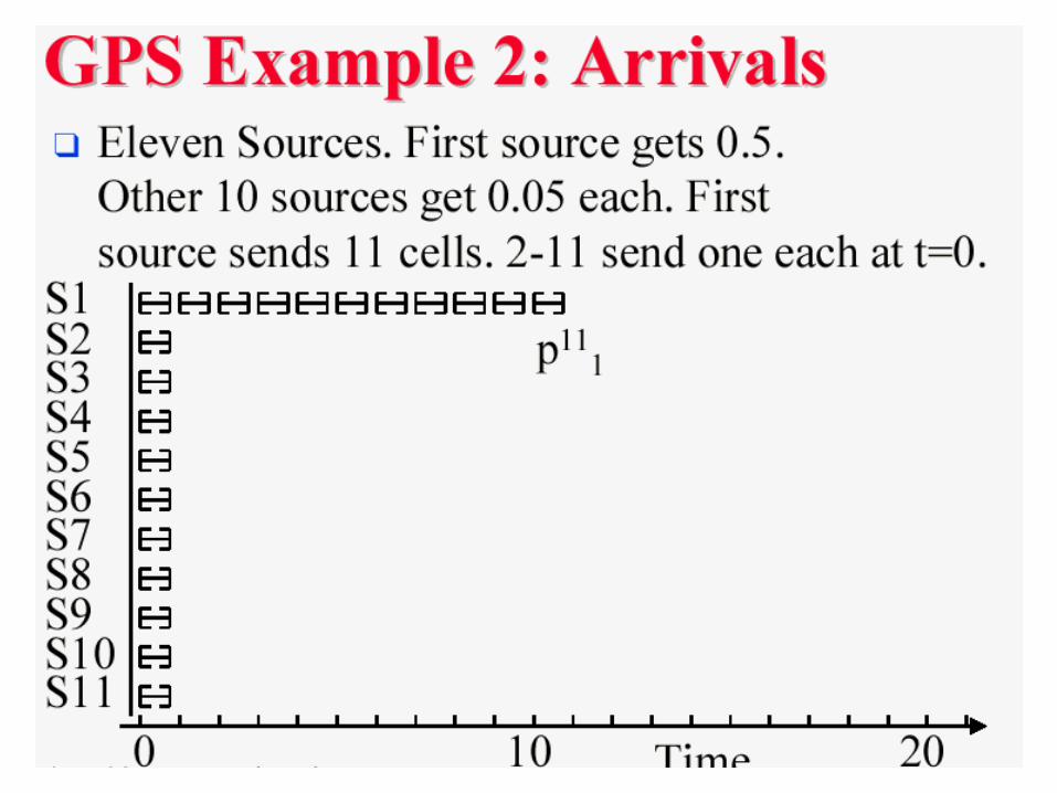
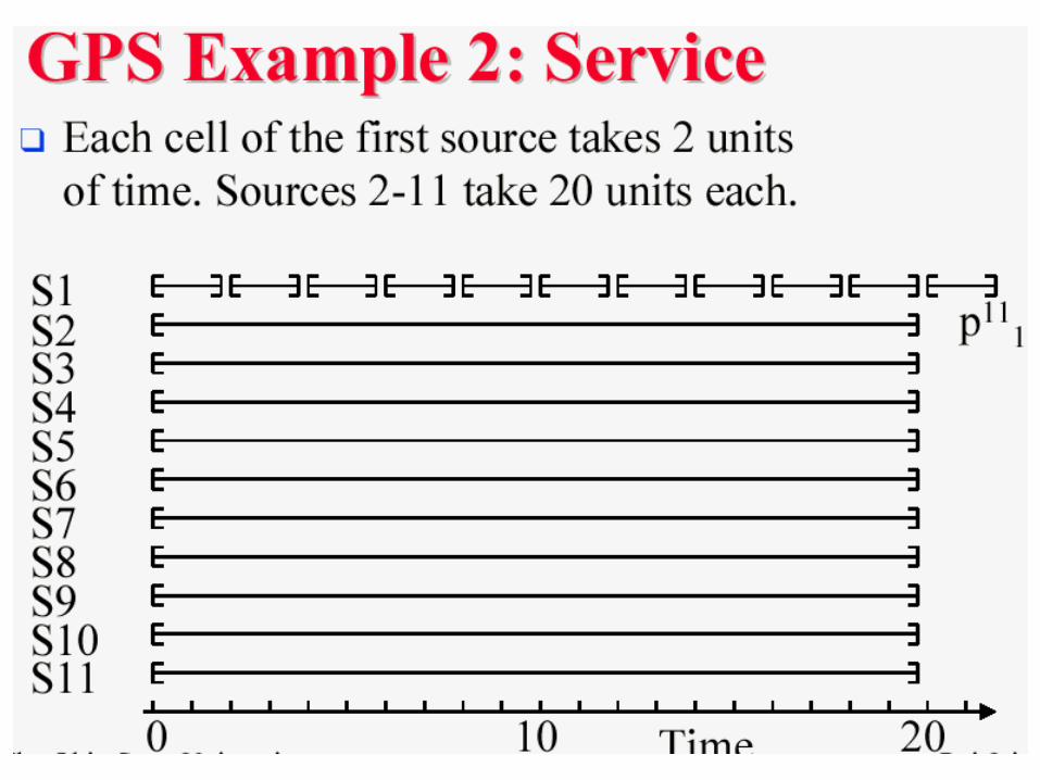
GPS: Example 2

GPS examlpe 2

0

5

10

15

20

25

time

queu

e si

ze A

B

C

5 15 3040 45

Packets: time 0 size 15 time 5 size 20 time 15 size 10

Lecture 4 #-23

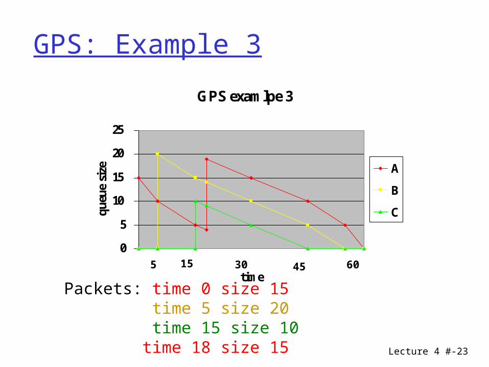
GPS: Example 3

GPS examlpe 3

0

5

10

15

20

25

time

queu

e si

ze A

B

C

5 15 30 45 60

Packets: time 0 size 15 time 5 size 20 time 15 size 10time 18 size 15

Lecture 4 #-24

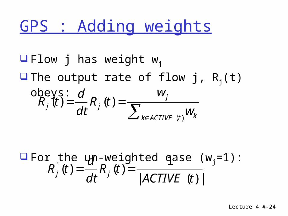
GPS : Adding weights

Flow j has weight wj

The output rate of flow j, Rj(t) obeys:

For the un-weighted case (wj=1):

)(

' )()(tACTIVEk k

jjj w

wtR

dt

dtR

|)(|

1)()('

tACTIVEtR

dt

dtR jj

Lecture 4 #-25

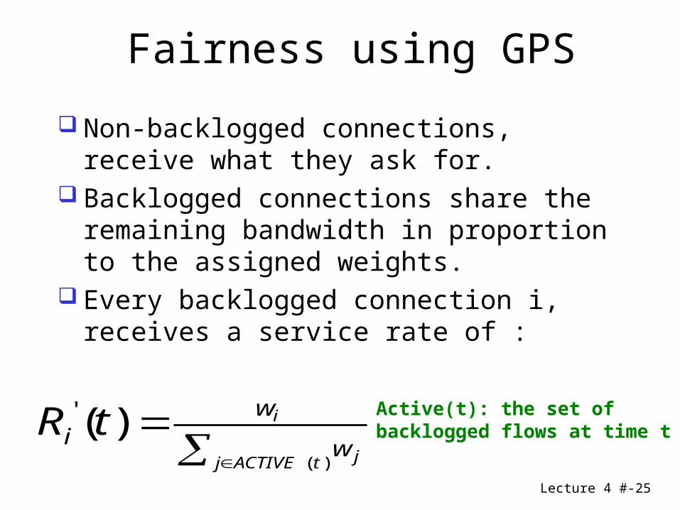
Non-backlogged connections, receive what they ask for.

Backlogged connections share the remaining bandwidth in proportion to the assigned weights.

Every backlogged connection i, receives a service rate of :

Fairness using GPS

)(

)('tACTIVEj j

i

w

wi tR Active(t): the set of

backlogged flows at time t

Lecture 4 #-26

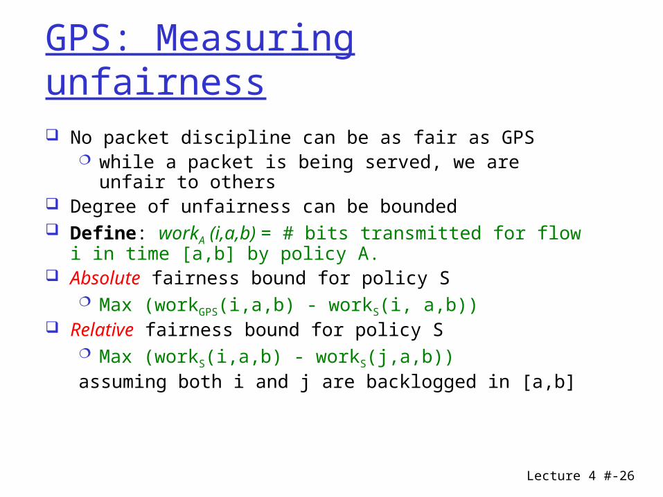
GPS: Measuring unfairness

No packet discipline can be as fair as GPS while a packet is being served, we are unfair to

others Degree of unfairness can be bounded Define: workA (i,a,b) = # bits transmitted for flow i in

time [a,b] by policy A. Absolute fairness bound for policy S

Max (workGPS(i,a,b) - workS(i, a,b)) Relative fairness bound for policy S

Max (workS(i,a,b) - workS(j,a,b))assuming both i and j are backlogged in [a,b]

Lecture 4 #-27

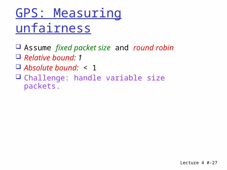
GPS: Measuring unfairness

Assume fixed packet size and round robin Relative bound: 1 Absolute bound: < 1 Challenge: handle variable size packets.

Lecture 4 #-28

Weighted Fair Queueing

Lecture 4 #-29

GPS to WFQ

We can’t implement GPS So, lets see how to emulate it We want to be as fair as possible But also have an efficient implementation

Lecture 4 #-30

Lecture 4 #-31

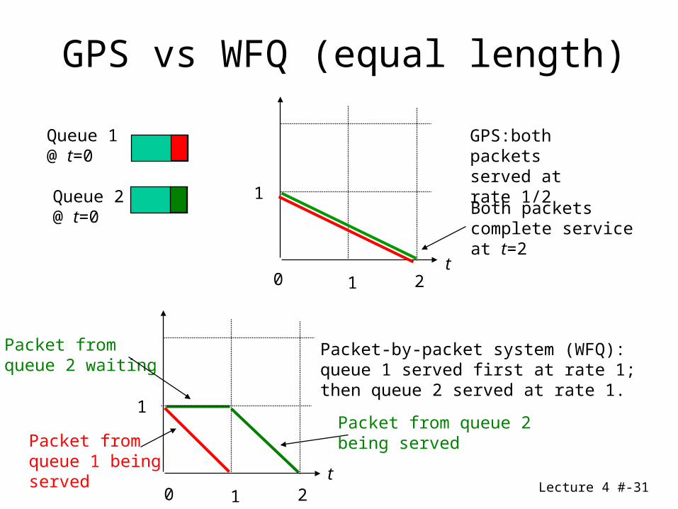
Queue 1@ t=0

Queue 2@ t=0

GPS:both packets served at rate 1/2

Both packets complete service at t=2

t

1

1 20

Packet-by-packet system (WFQ):queue 1 served first at rate 1;then queue 2 served at rate 1.

Packet fromqueue 1 beingserved

Packet from queue 2being served

Packet fromqueue 2 waiting

1

t1 20

GPS vs WFQ (equal length)

Lecture 4 #-32

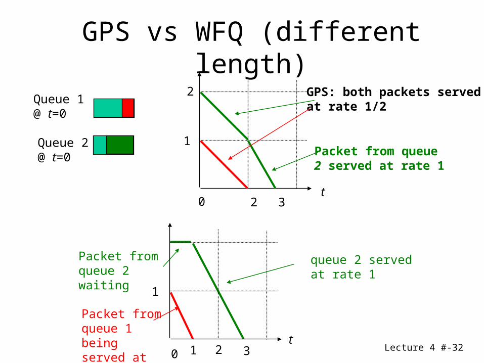
Queue 1@ t=0

Queue 2@ t=0

2

1

t30

2

Packet from queue2 served at rate 1

GPS: both packets served at rate 1/2

queue 2 served at rate 1

Packet fromqueue 1 beingserved at rate 1

Packet fromqueue 2 waiting

1

t1 20 3

GPS vs WFQ (different length)

Lecture 4 #-33

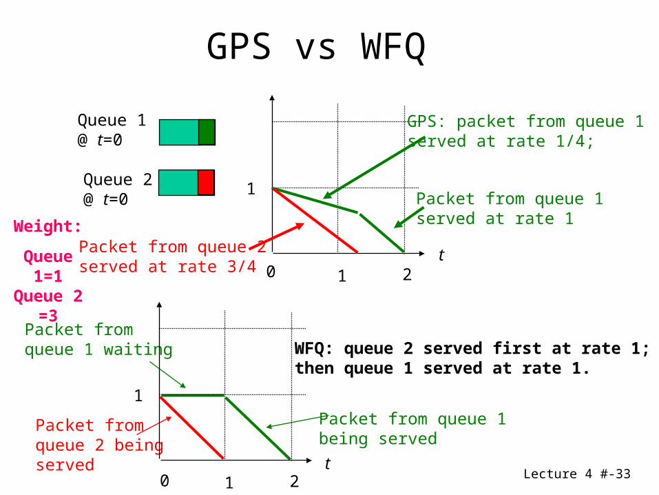
Queue 1@ t=0

Queue 2@ t=0

1

t1 20

WFQ: queue 2 served first at rate 1;then queue 1 served at rate 1.

Packet from queue 1being served

Packet fromqueue 2 beingserved

Packet fromqueue 1 waiting

1

t1 20

GPS: packet from queue 1served at rate 1/4;

Packet from queue 2served at rate 3/4

GPS vs WFQ

Weight:

Queue 1=1 Queue 2 =3

Packet from queue 1 served at rate 1

Lecture 4 #-34

Completion times

Emulating a policy: Assign each packet p a value time(p). Send packets in order of time(p).

FIFO: Arrival of a packet p from flow j:

last = last + size(p);time(p)=last;

perfect emulation...

Lecture 4 #-35

Round Robin Emulation

Round Robin (equal size packets) Arrival of packet p from flow j: last(j) = last(j)+ 1; time(p)=last(j);

Idle queue not handle properly!!! Sending packet q: round = time(q) Arrival: last(j) = max{round,last(j)}+ 1 time(p)=last(j);

What kind of low level scheduling?

Lecture 4 #-36

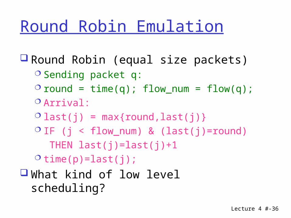
Round Robin Emulation

Round Robin (equal size packets) Sending packet q: round = time(q); flow_num = flow(q); Arrival: last(j) = max{round,last(j)} IF (j < flow_num) & (last(j)=round)

THEN last(j)=last(j)+1 time(p)=last(j);

What kind of low level scheduling?

Lecture 4 #-37

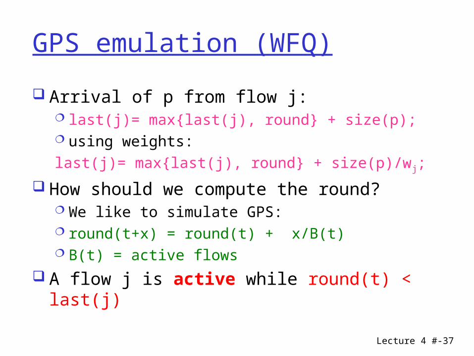
GPS emulation (WFQ)

Arrival of p from flow j: last(j)= max{last(j), round} + size(p); using weights:last(j)= max{last(j), round} + size(p)/wj;

How should we compute the round? We like to simulate GPS: round(t+x) = round(t) + x/B(t) B(t) = active flows

A flow j is active while round(t) < last(j)

Lecture 4 #-38

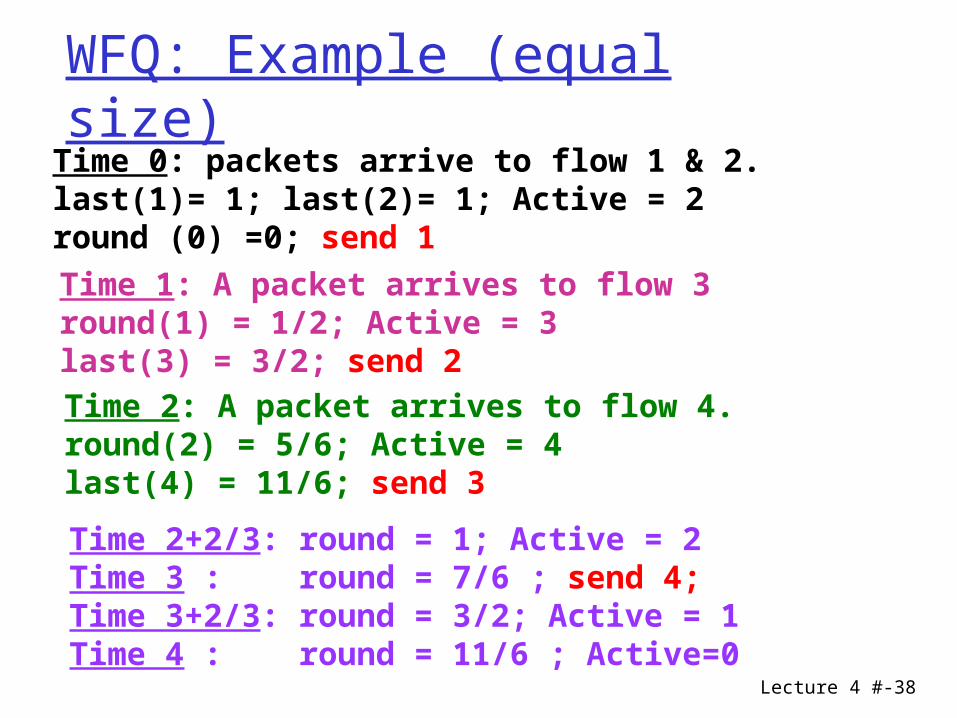
WFQ: Example (equal size)Time 0: packets arrive to flow 1 & 2.last(1)= 1; last(2)= 1; Active = 2round (0) =0; send 1

Time 1: A packet arrives to flow 3round(1) = 1/2; Active = 3last(3) = 3/2; send 2Time 2: A packet arrives to flow 4.round(2) = 5/6; Active = 4 last(4) = 11/6; send 3

Time 2+2/3: round = 1; Active = 2Time 3 : round = 7/6 ; send 4; Time 3+2/3: round = 3/2; Active = 1Time 4 : round = 11/6 ; Active=0

Lecture 4 #-39

Worst Case Fair Weighted Fair Queuing (WF2Q)

Lecture 4 #-40

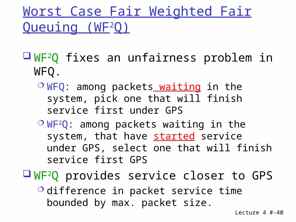
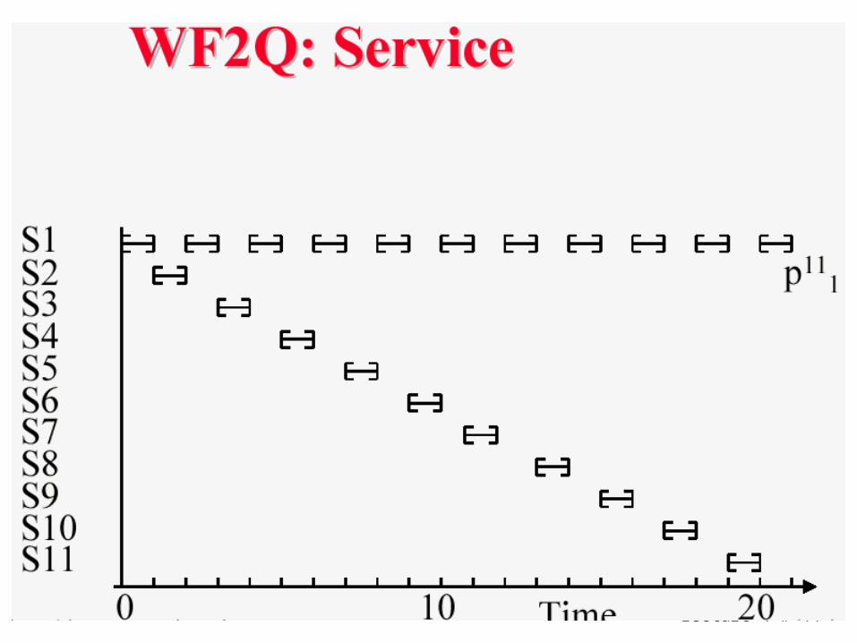
Worst Case Fair Weighted Fair Queuing (WF2Q)

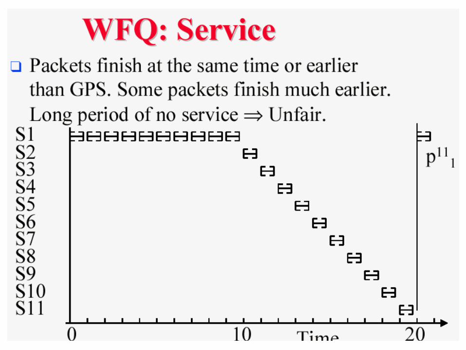
WF2Q fixes an unfairness problem in WFQ. WFQ: among packets waiting in the system,

pick one that will finish service first under GPS

WF2Q: among packets waiting in the system, that have started service under GPS, select one that will finish service first GPS

WF2Q provides service closer to GPS difference in packet service time bounded by

max. packet size.

Lecture 4 #-41

Lecture 4 #-42

Lecture 4 #-43

Lecture 4 #-44

Lecture 4 #-45

Multiple Buffers

Lecture 4 #-46

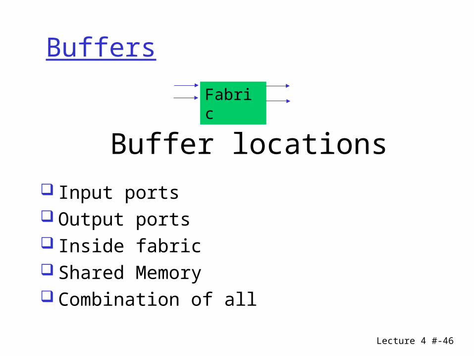
Buffers

Input ports Output ports Inside fabric Shared Memory Combination of all

Buffer locations

Fabric

Lecture 4 #-47

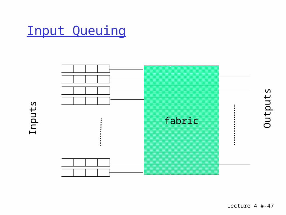
Input Queuing

fabric

Inp

uts

Outp

uts

Lecture 4 #-48

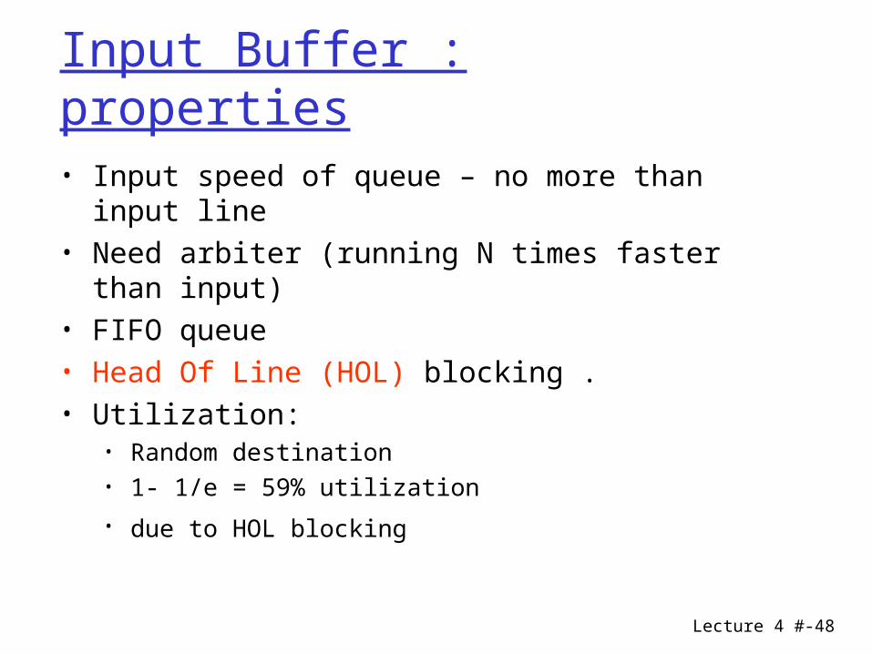
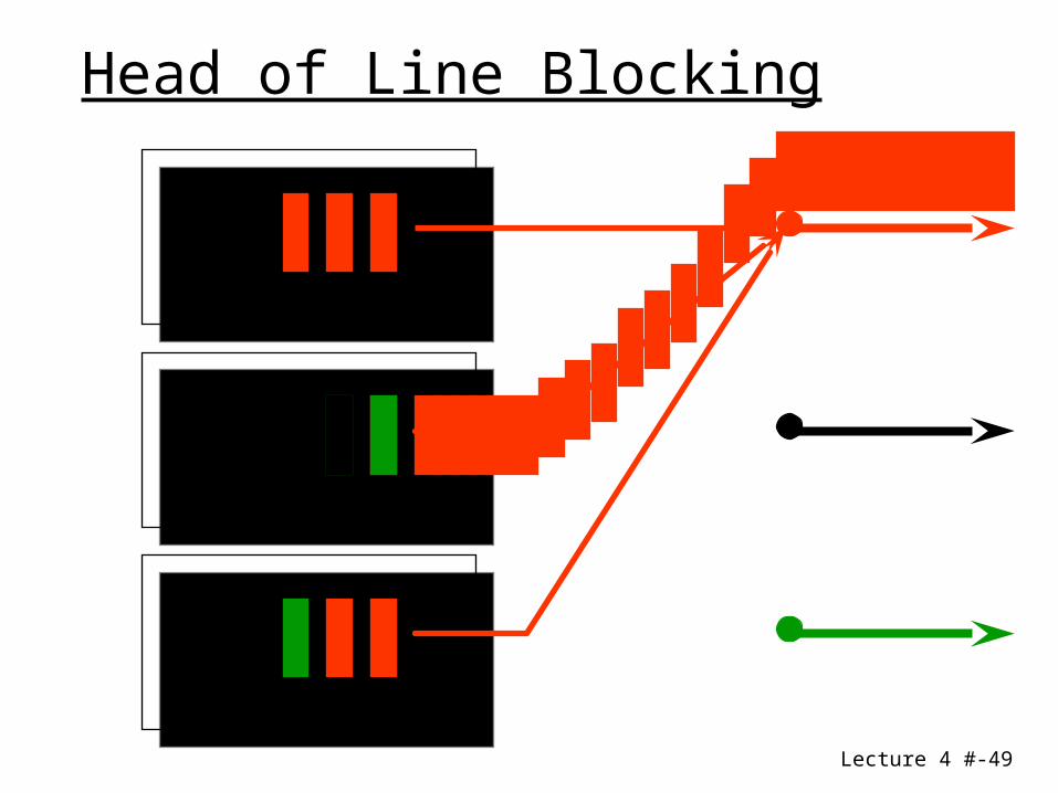
• Input speed of queue – no more than input line• Need arbiter (running N times faster than

input)• FIFO queue • Head Of Line (HOL) blocking .• Utilization:

• Random destination• 1- 1/e = 59% utilization

• due to HOL blocking

Input Buffer : properties

Lecture 4 #-49

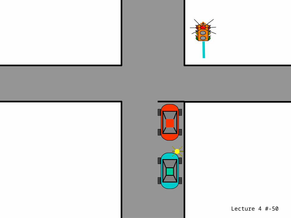
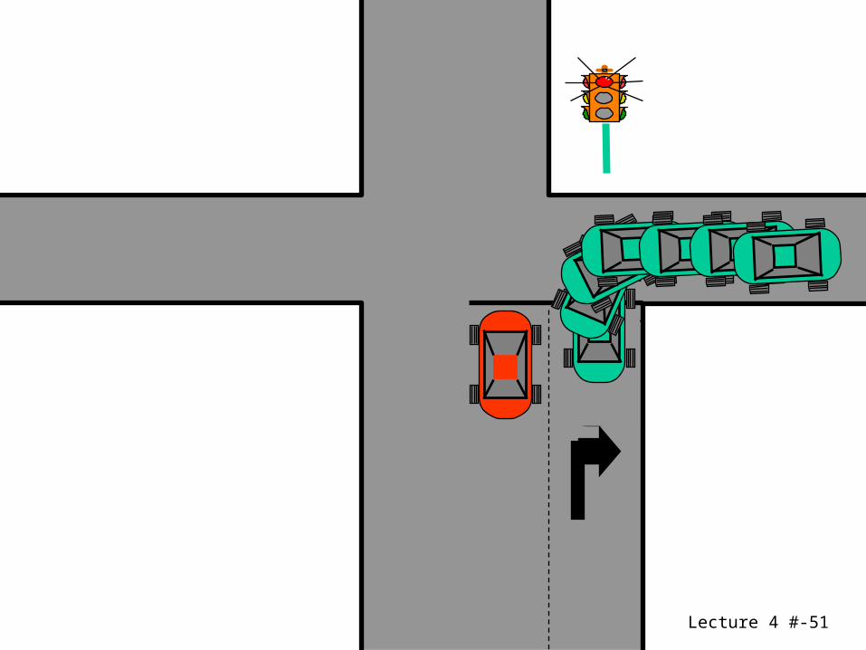
Head of Line Blocking

Lecture 4 #-50

Lecture 4 #-51

Lecture 4 #-52

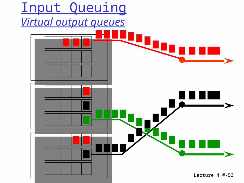
The fabric looks ahead into the input buffer for packets that may be transferred if they were not blocked by the head of line.

Improvement depends on the depth of the look ahead.

This corresponds to virtual output queues where each input port has buffer for each output port.

Overcoming HOL blocking: look-ahead

Lecture 4 #-53

Input QueuingVirtual output queues

Lecture 4 #-54

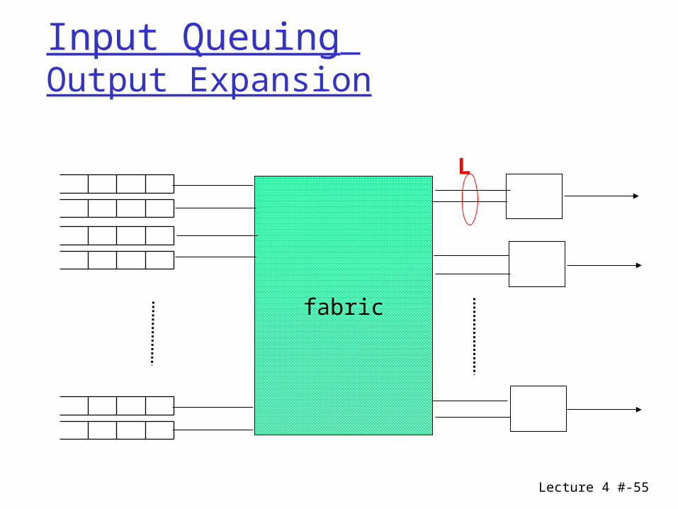
Each output port is expanded to L output ports

The fabric can transfer up to L packets to the same output instead of one cell.

Overcoming HOL blocking: output expansion

Karol and Morgan, IEEE transaction on communication, 1987: 1347-1356

Lecture 4 #-55

fabric

L

Input Queuing Output Expansion

Lecture 4 #-56

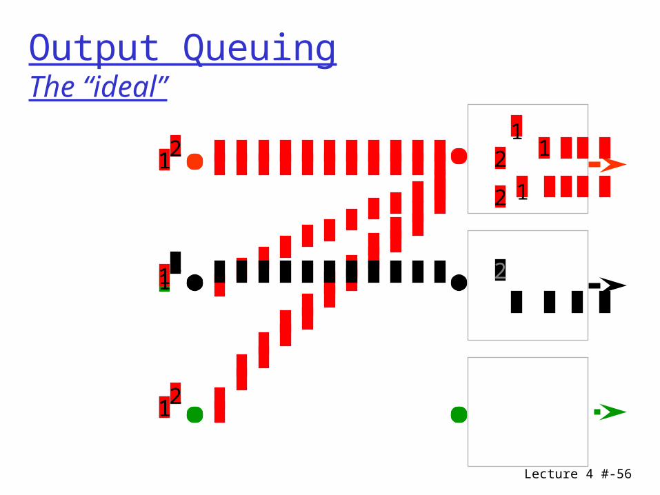
Output QueuingThe “ideal”

1

1

1

1

1

1

1

1

1

11

1

2

2

2

2

2

2

Lecture 4 #-57

Output Buffer : properties

No HOL problem Output queue needs to run faster than input lines Need to provide for N packets arriving to same

queue solution: limit the number of input lines that can

be destined to the output.

Lecture 4 #-58

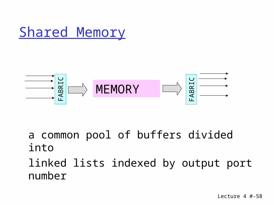
Shared Memory

a common pool of buffers divided into

linked lists indexed by output port number

FAB

RIC

FAB

RIC

MEMORY

Lecture 4 #-59

Shared Memory: properties

• Packets stored in memory as they arrive• Resource sharing• Easy to implement priorities• Memory is accessed at speed equal to sum of

the input or output speeds• How to divide the space between the sessions