lecture 29 –introduction to finite elements methods (cont.)

Lecture 29 – Introduction to finite elements methods (cont.)

Instructor: Prof. Marcial Gonzalez

Fall, 2021ME 323 – Mechanics of Materials

Last modified: 8/16/21 9:24:07 AM

News: _____

Introduction to finite element methods (FEM)

3

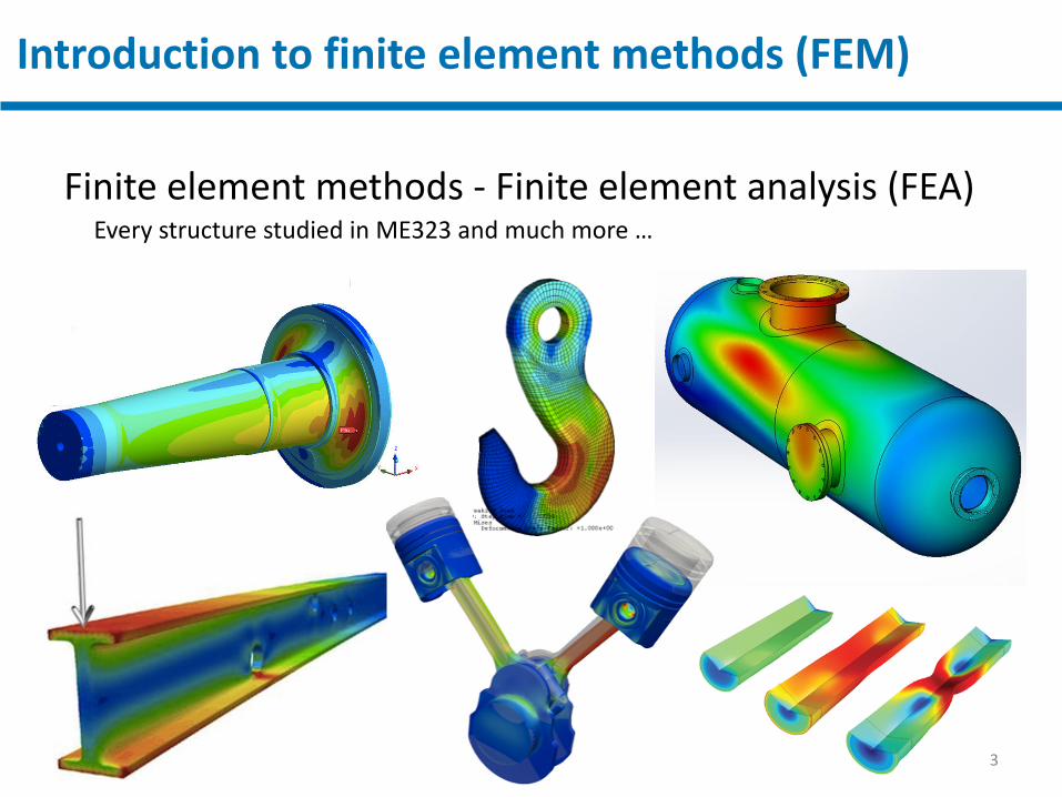
Finite element methods - Finite element analysis (FEA)Every structure studied in ME323 and much more …


4

Finite element methods – One-dimensional rod elements- We obtain the equilibrium solution using an energy principle

Principle of minimum potential energy“For a given set of admissible displacement fields for a conservative system,an equilibrium state of the system will correspond to a state for which thetotal potential energy is stationary.”

+ An admissible displacement field for a rod is one that satisfies all of thedisplacement boundary conditions of the problem.

+ The total potential energy of the system is equal to the sum of the potential ofthe applied external forces and the strain energy in the rod.

+ Stationarity of the potential energy correspond to its minimization with respectto the displacement field.

for each node in the mesh


5

Finite element methods – One-dimensional rod elements- Example 55 (review):

Number of nodes: 4

Number of elements: 3

Boundary conditions:

Stiffness of each element:


6

Finite element methods – One-dimensional rod elements- Example 55, solved in 5 steps+ Step #1: Identify the degrees of freedom

+ Step #2: Build the global stiffness matrix

Number of nodes: 4Number of elements: 3


7

Finite element methods – One-dimensional rod elements- Example 55, solved in 5 steps+ Step #3: Enforce boundary conditions

+ Step #4: Solve the reduced system of linear equations



8

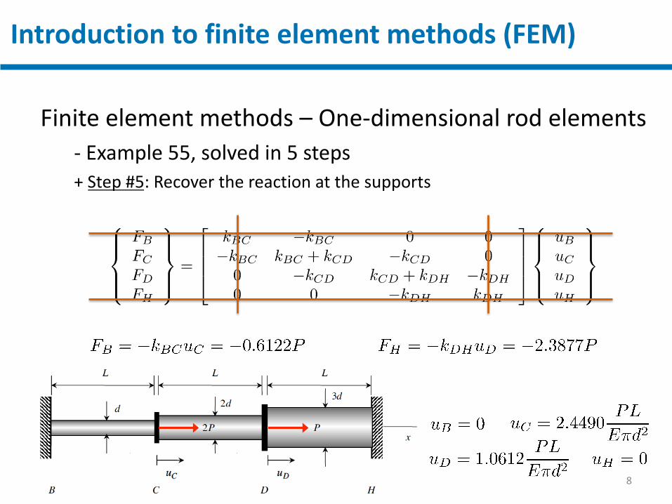
Finite element methods – One-dimensional rod elements- Example 55, solved in 5 steps+ Step #5: Recover the reaction at the supports


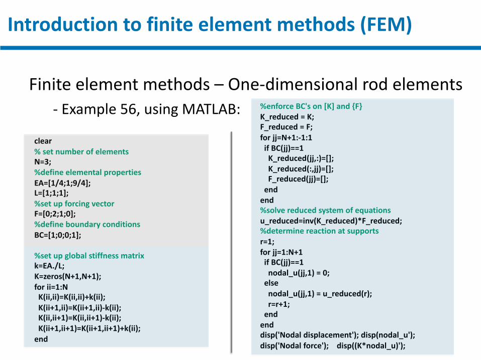
Finite element methods – One-dimensional rod elements- Example 56, using MATLAB:

clear% set number of elementsN=3;%define elemental propertiesEA=[1/4;1;9/4];L=[1;1;1];%set up forcing vectorF=[0;2;1;0];%define boundary conditionsBC=[1;0;0;1];

%set up global stiffness matrixk=EA./L;K=zeros(N+1,N+1);for ii=1:N

K(ii,ii)=K(ii,ii)+k(ii);K(ii+1,ii)=K(ii+1,ii)-k(ii);K(ii,ii+1)=K(ii,ii+1)-k(ii);K(ii+1,ii+1)=K(ii+1,ii+1)+k(ii);

end

%enforce BC's on [K] and {F}K_reduced = K;F_reduced = F;for jj=N+1:-1:1

if BC(jj)==1K_reduced(jj,:)=[];K_reduced(:,jj)=[];F_reduced(jj)=[];

endend%solve reduced system of equationsu_reduced=inv(K_reduced)*F_reduced;%determine reaction at supportsr=1;for jj=1:N+1

if BC(jj)==1nodal_u(jj,1) = 0;

elsenodal_u(jj,1) = u_reduced(r);r=r+1;

endenddisp('Nodal displacement'); disp(nodal_u');disp('Nodal force'); disp((K*nodal_u)');


10

Finite element methods – One-dimensional rod elements- Example 56: (5 nodes)

clear% set number of elementsN=4;%define elemental propertiesEA=[(1+1)/2;(1+1)/2;(1+1.5)/2;(1.5+2)/2];L =[0.5 ;0.5 ;0.5 ;0.5 ];%set up forcing vectorF =[1;0;0;0;0];%define boundary conditionsBC=[0;0;0;0;1];

Nodal displacement 1.6857 1.1857 0.6857 0.2857 0

Nodal force1.0000 0 0.0000 -0.0000 -1.0000

Stiffness matrix2.0000 -2.0000 0 0 0

-2.0000 4.0000 -2.0000 0 00 -2.0000 4.5000 -2.5000 00 0 -2.5000 6.0000 -3.50000 0 0 -3.5000 3.5000



11


Nodal displacement 1.6898 1.1898 0.6898 0.4040 0.1818 0

Nodal force1.0000 -0.0000 0 -0.0000 0.0000 -1.0000

Stiffness matrix2.0000 -2.0000 0 0 0 0

-2.0000 4.0000 -2.0000 0 0 00 -2.0000 5.5000 -3.5000 0 00 0 -3.5000 8.0000 -4.5000 00 0 0 -4.5000 10.0000 -5.50000 0 0 0 -5.5000 5.5000

clear% set number of elementsN=5;%define elemental propertiesEA=[1 ;1 ;(1+4/3)/2;(4/3+5/3)/2;(5/3+2)/2];L =[0.5 ;0.5 ;1/3 ;1/3 ;1/3 ];%set up forcing vectorF =[1;0;0;0;0;0];%define boundary conditionsBC=[0;0;0;0;0;1];



12

Finite element methods – One-dimensional rod elements- Example 56: (3 to N nodes)

Num Elements | Displ. Node 13.0000 1.66674.0000 1.68575.0000 1.68986.0000 1.69127.0000 1.69198.0000 1.69239.0000 1.6925

10.0000 1.692711.0000 1.692812.0000 1.692813.0000 1.692914.0000 1.692915.0000 1.693016.0000 1.693017.0000 1.693018.0000 1.693019.0000 1.693020.0000 1.693121.0000 1.693122.0000 1.693123.0000 1.6931

Rela

tive

erro

r in

the

solu

tion

Number of elements

Slope of 2(quadratic convergence!)


13


Nodal displacement0.3979 0 -0.1413 -0.2941 -2.5409

Nodal force1.0000 2.0000 0.0000 -0.0000 -3.0000

Stiffness matrix2.5133 -2.5133 0 0 0

-2.5133 23.7504 -21.2372 0 00 -21.2372 40.8721 -19.6350 00 0 -19.6350 20.9701 -1.33520 0 0 -1.3352 1.3352

clear% set number of elementsN=4;%define elemental properties (A=pi*D^2/4)EA=pi/4*[4.00^2;5.20^2;5.00^2;(5.00^2+3.00^2)/2];L =[5.00;1.00;1.00;10.00];%set up forcing vectorF =[1; 0; 0; 0; -3];%define boundary conditionsBC=[0; 1; 0; 0; 0];

0 1 2 3 4 5 6 7 8 9 10 11 12 13 14 15 16 17


14


Nodal displacement0.3979 0 -0.1413 -0.2941 -1.2257 -2.7536

Nodal force1.0000 2.0000 0 0 -0.0000 -3.0000

Stiffness matrix2.5133 -2.5133 0 0 0 0

-2.5133 23.7504 -21.2372 0 0 00 -21.2372 40.8721 -19.6350 0 00 0 -19.6350 22.8551 -3.2201 00 0 0 -3.2201 5.1836 -1.96350 0 0 0 -1.9635 1.9635

clear% set number of elementsN=5;%define elemental properties (A=pi*D^2/4)EA=pi/4*[4^2;5.2^2;5^2;(5^2+4^2)/2;(4^2+3^2)/2];L =[5.00;1.00;1.00;5.00;5.00];%set up forcing vectorF =[1; 0; 0; 0; 0; -3];%define boundary conditionsBC=[0; 1; 0; 0; 0; 0];

0 1 2 3 4 5 6 7 8 9 10 11 12 13 14 15 16 17


15

Finite element methods – One-dimensional rod elements- Example 58:

Answer:

Any questions?

16


lecture 29 –introduction to finite elements methods (cont.)

Documents