analysis of finite elements and finite differences for...
TRANSCRIPT
Mathematics and Computers in Simulation 34 (1992) 141-161
North-Holland
141
MATCOM 910
Analysis of finite elements and finite differences for shallow water equations: A review B. Neta
Department of Mathematics, Nar,al Postgraduate School, Monterey, CA 93943, United States
Abstract
Neta, B., Analysis of finite elements and finite differences for shallow water equations: A review, Mathematics and Computers in Simulation 34 (1992) 141-161.
In this review article we discuss analyses of finite-element and finite-difference approximations of the shallow water equations. An extensive bibliography is given.
0. Introduction
In this article we review analyses of finite-element and finite-difference methods for the approximation of the shallow water equations. Results by the author and others are given, tables showing side by side all these results are included. Current research including semi- Lagrangian and domain decomposition methods are covered. An extensive bibliography is given.
1. Shallow water equations
1.1. Model
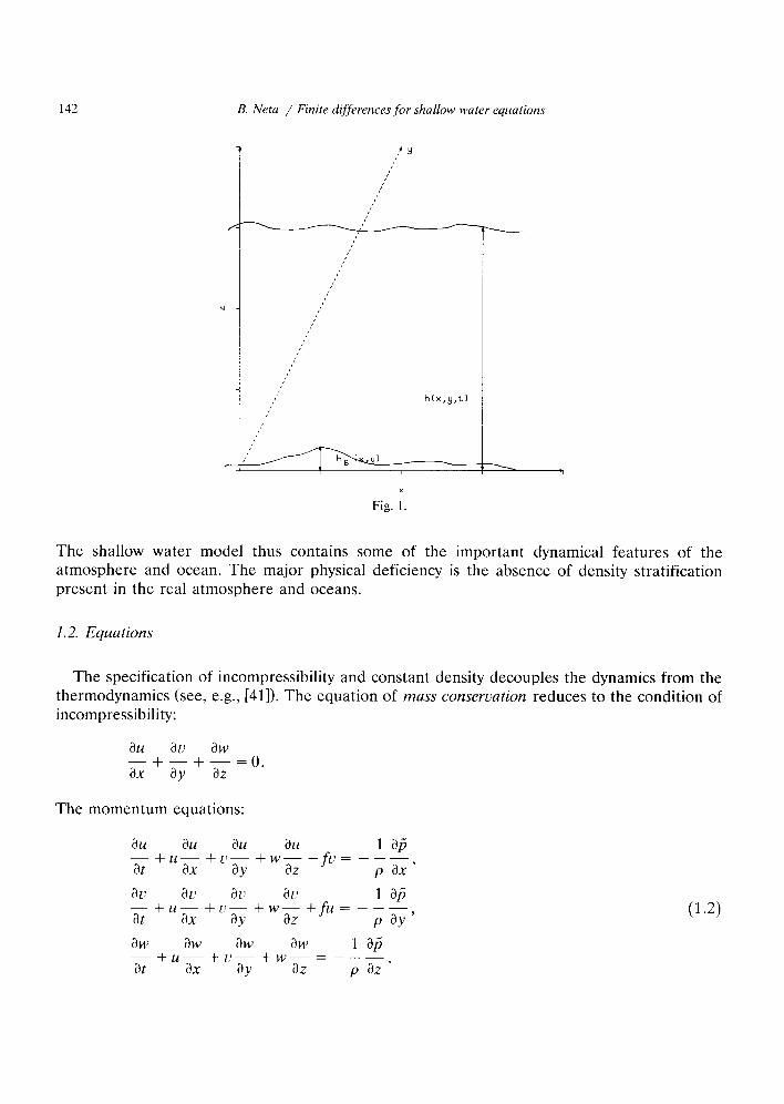
Consider a sheet of fluid with constant and uniform density (see, for example, [41]). (See Fig. 1.) The height of the surface of the fluid above the reference level z = 0 is h(x, y, t). With atmosphere or ocean in mind, we model the body force arising from the potential 4 =gh. The rigid bottom is defined by the surface z = h,(x, y>. The velocity has components u, L’ and w in the X-, y- and z-directions, respectively. The pressure of the fluid surface can be arbitrarily imposed, but here we assume it is constant. The fluid is assumed inciscid, that is, only motions for which viscosity is unimportant are considered.
Let H be the average depth of the fluid, h - h,. Let L be a characteristic horizontal scale for the motion. For shallow water theory one must have
H - -=c 1. L (14
Correspondence to: Prof. B. Neta, Code MA/Nd, Department of Mathematics, Naval Postgraduate School, Montcrcy, CA 93943-5100, United States.
0378-4754/92/$05.00 0 1992 - Elsevier Science Publishers B.V. All rights reserved
142 B. Neta / Finite differences for shallow water equations
,’ !’
N - ,’ ,’
,’
,’
,’
h[x,y,tl
!’
I _
x
Fig. 1.
----. 7
The shallow water model thus contains some of the important dynamical features of the atmosphere and ocean. The major physical deficiency is the absence of density stratification present in the real atmosphere and oceans.
1.2. Equations
The specification of incompressibility and constant density decouples the dynamics from the thermodynamics (see, e.g., [41]). The equation of mass conservation reduces to the condition of incompressibility:
au aL! aw
G+-+az=O. ay
The momentum equations:
au au au au I aj t+uax+c-+w--g-fL~= --->
ay P ax ar; aL? au au I ag at+uax+“-+W~+fu=---,
ay P aY (14
aw aw aw aw 1 afi ~+u~+c-+w~=---_,
ay P az
B. Netu / Finite differences for shullow water equutions 143
where the total pressure p(x, y, z, t) is
P(.G Y, 2, t) = -Pi? +P(x, Y, 23 t>. (W
Note that the horizontal pressure gradient is independent of z if one uses the hydrostatic approximation
aP H2 -=--pg+o t (I 1) . dZ
Such approximation follows from scale analysis of the momentum equations and the pressibility condition. Integrating the last equation and using the boundary condition
P(X> Y> h) ‘PO
yields
P =m(h -4 +Po*
(1.4)
incom-
(I.9
(1.6)
This means that the pressure in excess of pO at any point simply equals the weight of the unit column of fluid above the point at that time.
Note that the horizontal pressure gradient is independent of z, therefore the horizontal accelerations must be independent of z. For low Rossby-wave number U/(fL), the Taylor- Proudman theorem (see, e.g., [41, p. 431) applied to a homogeneous fluid will require the velocities to be independent of z.
The vertical momentum equation can be integrated easily, since u and L’ are independent of
The condition of IZO normal flow at the bottom requires
ah, ah, w(x, y, h,, t) =uax fc-
ay .
This leads to
au a[:
i I ahE3 w(x, y, z, t) = (h, -z) z + - fur ay
(1.8)
ahI3 +tJ-.
ay (1.9)
The corresponding kinematic condition at the surface z = h is
ah ah ah
Thus
W(X, y, 2, t) = z +uz + L’-. ay
(1.10)
g + ;[a(h-h,J + y&h -h,)] =O. (1.11)
144 B. Neta / Finite differences for shallow water equations
This equation, combined with the horizontal momentum equations
au au au ah au ar; au ah -+Llx+L!ay‘-fL~=-_g~, at
~+"~+"-+fu=-g-
dY ay (1.12)
form the shallow water equations,
Remarks. (1) The vertical momentum equation can be interpreted as follows: if the local horizontal divergence of volume V . (U’H) is positive, it must be balanced by a local decrease of the layer thickness due to a drop in the free surface. Here we define the total depth H=h -h,.
(2) The time it takes a fluid element to move a distance L with speed U is L/U. If that period of time is much less than the period of rotation of the earth, the fluid can barely feel the earth’s rotation. For rotation to be important, we anticipate U/( fL) G 1. This ratio is called Rossby number.
2. Advection equation
Advective processes are dominant in atmospheric and oceanic circulation systems, while diffusive effects are important only in boundary layer regions. Any numerical model for these circulation systems should treat advective effects accurately. Neta and Williams [36] have analyzed various finite-element formulations of the linearized advection equation in two dimensions,
aF aF aF -+Vcosf9~+~sinH--0, at ay
(2.1)
where I/ is the mean flow speed and 13 is the direction relative to the x-axis. The analytic solution to (2.1) is
F(x, y, t) =F(x - tV cos 13, y - tV sin 8, 0). (2.2)
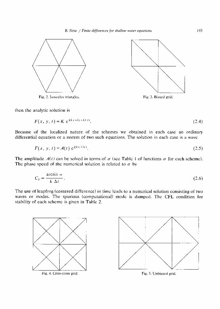
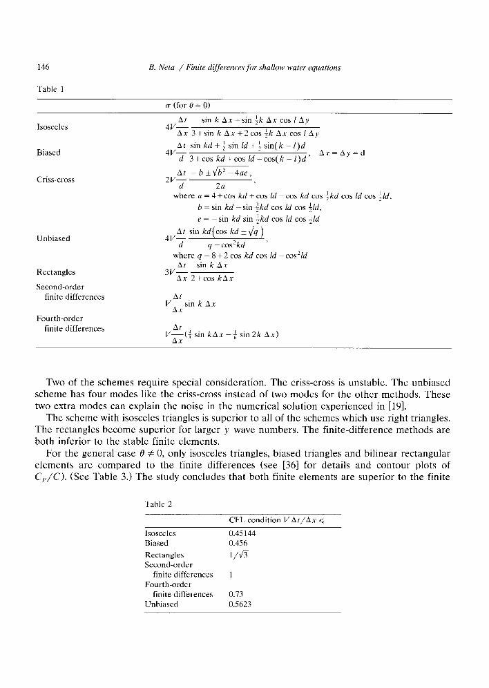
The following methods were analyzed: (i) linear elements on isosceles triangles;
(ii) linear elements on biased triangles; (iii) linear elements on criss-cross grid; (iv) linear elements on unbiased triangles; (v) bilinear basis functions on rectangles;
(vi) second-order finite differences; and (vii) fourth-order finite differences.
Figures 2-5 show various triangulations in the case Ax = Ay. The leapfrog time differencing is used in all cases. For the case 8 = 0 (flow in the x-axis
direction) one can show that if the initial condition is
F(x, y, 0) =K ej(kxi’y), (2.3)
B. Neta / Finite differences for shallow water equations 145
Fig. 2. Isosceles triangles. Fig. 3. Biased grid.
then the analytic solution is
Because of the localized nature of the schemes we obtained in each case an ordinary differential equation or a system of two such equations. The solution in each case is a wave
F(x, y, t) =A(t) ejck++ly). (2.5)
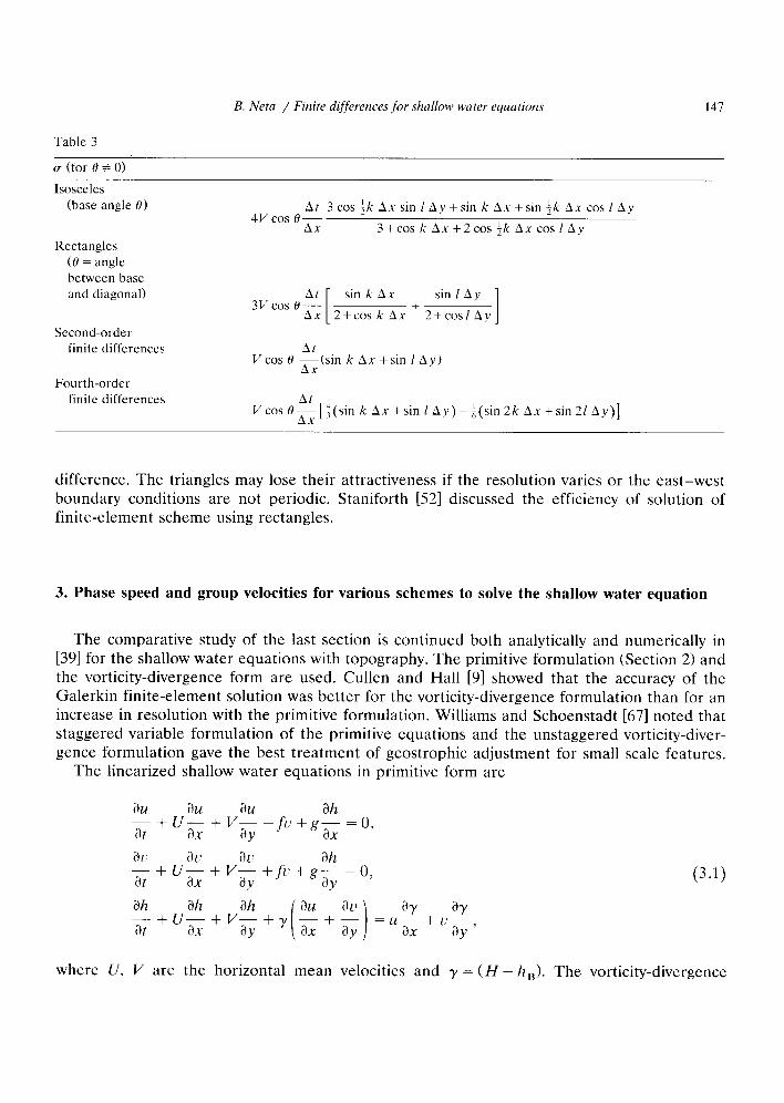
The amplitude A(t) can be solved in terms of (T (see Table 1 of functions u for each scheme). The phase speed of the numerical solution is related to (T by
arcsin (T c,=
kAt ’ P-6)
The use of leapfrog (centered difference) in time leads to a numerical solution consisting of two waves or modes. The spurious (computational) mode is damped. The CFL condition for stability of each scheme is given in Table 2.
Fig. 4. Criss-cross grid. Fig. 5. Unbiased grid.
146
Table 1
B. Neta / Finite differences for shallow water equations
(T (for 0 = 0)
Isosceles
Biased
4VF sin k Ax +sin ;k Ax cos 1 Ay
Ax 3+sin kAx+2cosikAxcoslAy
At sin kd + i sin Id + i sin( k - 1)d 4v-
d 3+coskd+cosld+cos(k-l)d’ Ax=Ay=d
Criss-cross At -bid=,
2vY? 2a ’ where a = 4 + cos kd + cos Id - cos kd cos fkd cos Id cos ild,
b = sin kd -sin $kd cos Id cos $d,
e = -sin kd sin ikd cos Id cos $d
Unbiased
Rectangles
Second-order finite differences
Fourth-order
4vE sin kd(cos kd f 6)
d q -cos’kd ’ where q = 8 + 2 cos kd cos Id - cos’ld
At sinkAx 3v-
Ax 2+cos kAx
At Vzsin k Ax
finite differences Vg($ sin kAx -i sin 2k Ax)
Two of the schemes require special consideration. The criss-cross is unstable. The unbiased scheme has four modes like the criss-cross instead of two modes for the other methods. These two extra modes can explain the noise in the numerical solution experienced in [19].
The scheme with isosceles triangles is superior to all of the schemes which use right triangles. The rectangles become superior for larger y wave numbers. The finite-difference methods are both inferior to the stable finite elements.
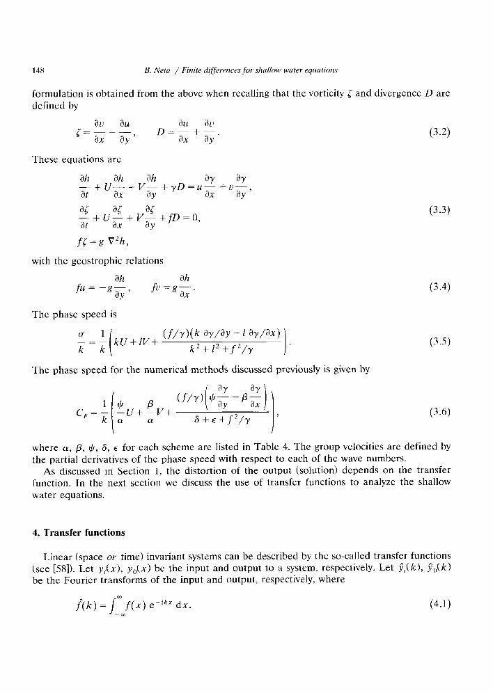
For the general case 8 # 0, only isosceles triangles, biased triangles and bilinear rectangular elements are compared to the finite differences (see [36] for details and contour plots of C,/C>. (See Table 3.) The study concludes that both finite elements are superior to the finite
Table 2
CFL condition V At/Ax <
Isosceles 0.45144 Biased 0.456
Rectangles l/6 Second-order
finite differences 1 Fourth-order
finite differences 0.73 Unbiased 0.5623
B. Neta / Finite differences for shallow water equations 147
Table 3
g (for 0 # 0)
Isosceles
(base angle 0)
Rectangles
At 3 cos ik Ax sin 1 Ay +sin k Ax +sin ik Ax cos 1 Ay 4vcos ex
3+cos k Ax +2cos ;k Ax cos 1 Ay
(0 = angle between base and diagonal)
Second-order finite differences
Fourth-order
3v cos 0’ [
sin k Ax sin 1 Ay
Ax 2+cos k Ax +
2+cosl Ay 1 Vcos 0 g(sin k Ax +sin 1 Ay)
finite differences
difference. The triangles may lose their attractiveness if the resolution varies or the east-west boundary conditions are not periodic. Staniforth [52] discussed the efficiency of solution of finite-element scheme using rectangles.
3. Phase speed and group velocities for various schemes to solve the shallow water equation
The comparative study of the last section is continued both analytically and numerically in [39] for the shallow water equations with topography. The primitive formulation (Section 2) and the vorticity-divergence form are used. Cullen and Hall [9] showed that the accuracy of the Galerkin finite-element solution was better for the vorticity-divergence formulation than for an increase in resolution with the primitive formulation. Williams and Schoenstadt [67] noted that staggered variable formulation of the primitive equations and the unstaggered vorticity-diver- gence formulation gave the best treatment of geostrophic adjustment for small scale features.
The linearized shallow water equations in primitive form are
(3.1)
where U, I/ are the horizontal mean velocities and y = (H - h,). The vorticity-divergence
14s B. Neta / Finite differences for shallow water equations
formulation is obtained from the above when recalling that the vorticity l and divergence D are defined by
These equations are
ah ah ah ay dY at+uax+v-+yD=u~+“-’
ay ay
fY=s V2h,
with the geostrophic relations
fu = -g;, fvg$
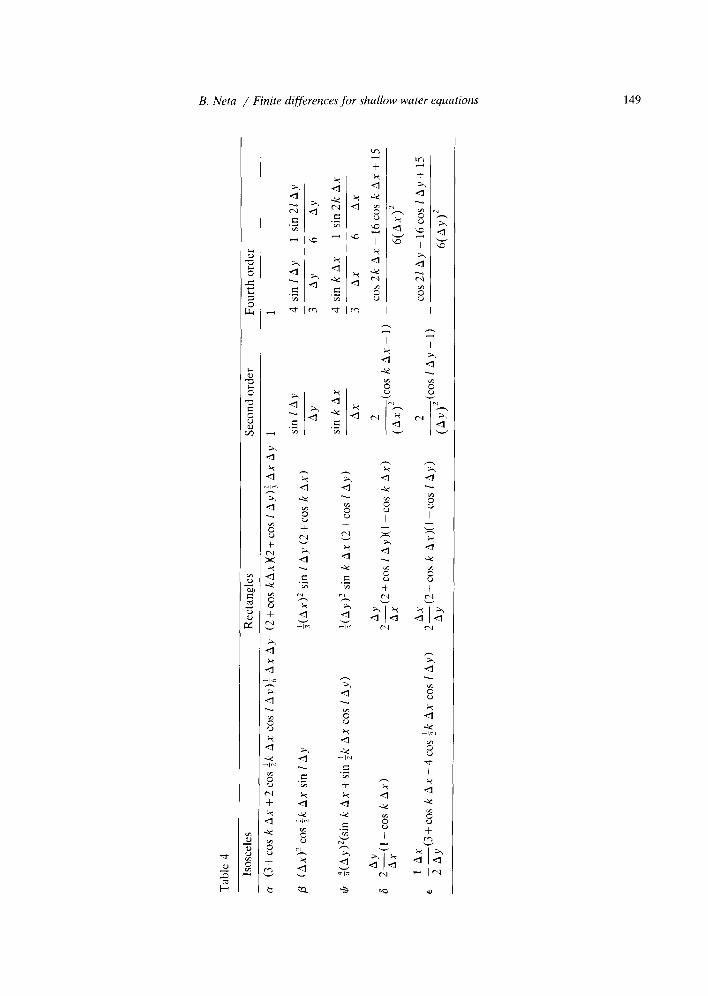
The phase speed is
(T 1 _=_ k k
kU+ lI/+ (f/Y)@ aY/aY - 1 aY/ax)
k2+12+f2/y
The phase speed for the numerical methods discussed previously is given by
1 cc, C”=k -u+%+ 1
WY)( *z -$) ff LY I 6+e+f2/y ’
(3.3)
(3.4)
(3.5)
(3.6)
where cy, p, $, 6, E for each scheme are listed in Table 4. The group velocities are defined by the partial derivatives of the phase speed with respect to each of the wave numbers.
As discussed in Section 1, the distortion of the output (solution) depends on the transfer function. In the next section we discuss the use of transfer functions to analyze the shallow water equations.
4. Transfer functions
Linear (space or time) invariant systems can be described by the so-called transfer functions (see [SS]). Let yi(x), yO(x) be the input and output to a system, respectively. Let y^Jk), y,,(k)
be the Fourier transforms of the input and output, respectively, where
fjk) = jrn f(x) eeikx dx. -02
(4.1)
B. Netu / Finite differences for shallow water equations 149
150 B. Neta / Finite differences for shallow water equations
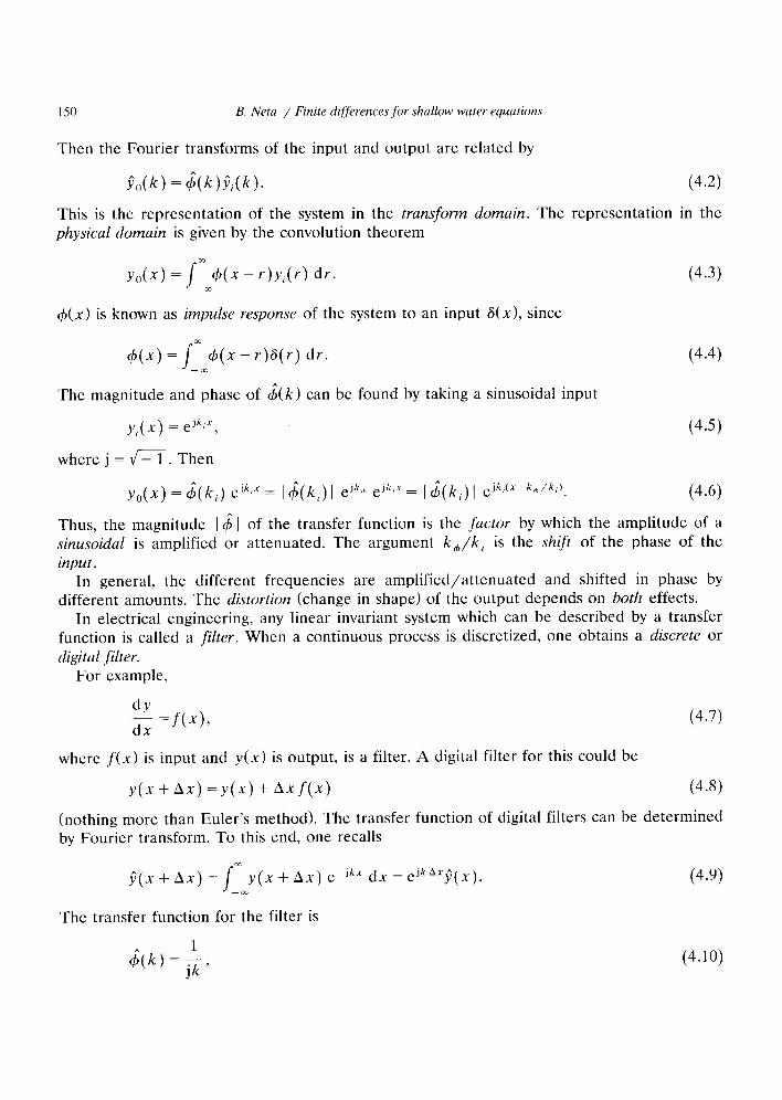
Then the Fourier transforms of the input and output are related by
9{J(k) = J(k)Fi(k)’ (4.2)
This is the representation of the system in the transform domain. The representation in the physical domain is given by the convolution theorem
d( x> is known as impulse response of the system to an input 6(x), since
+(x) = lrn 4(x - Y)~(Y) dr. -cc
(4.3)
(4.4)
The magnitude and phase of J(k) can be found by taking a sinusoidal input
yi( x) = ejkd.r,
where j = \r-1. Then
(4.5)
y,,(x) = $(k,) ejk? = 1 $(ki) 1 ejkcb ejk,x = 1 $(k,) 1 ejk#(x+kcb/kt). (4.6)
Thus, the magnitude 141 of the transfer function is the factor by which the amplitude of a sinusoidal is amplified or attenuated. The argument k,/k, is the shift of the phase of the input.
In general, the different frequencies are amplified/attenuated and shifted in phase by different amounts. The distortion (change in shape) of the output depends on both effects.
In electrical engineering, any linear invariant system which can be described by a transfer function is called a filter. When a continuous process is discretized, one obtains a discrete or
digital filter.
For example,
2 =f(x), WI
where f(x) is input and y(x) is output, is a filter. A digital filter for this could be
y(x + Ax) =y(x) + Axf(x) (4.8)
(nothing more than Euler’s method). The transfer function of digital filters can be determined by Fourier transform. To this end, one recalls
y^(x + Ax) = /m y(x + Ax) e-jkx dx = ejkAxy^(x). (4.9) --CD
The transfer function for the filter is
6(k) = ;> (4.10)
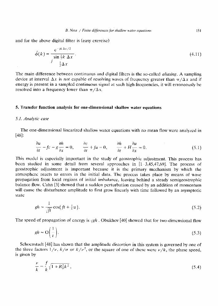
B. Neta / Finite differences for shallow water equations 151
and for the above digital filter is (easy exercise)
(6”(k) =
e-jk Ax/2
sin ik Ax ’ (4.11)
j ;Ax
The main difference between continuous and digital filters is the so-called aliasing. A sampling device at interval Ax is not capable of resolving waves of frequency greater than r/Ax and if energy is present in a sampled continuous signal at such high frequencies, it resolved into a frequency lower than n/Ax.
5. Transfer function analysis for one-dimensional shallow water equations
5.1. Analytic case
will erroneously be
The one-dimensional linearized shallow water equations with no mean flow were analyzed in [48]:
; +fu = 0, dh ;+H;=O. (5.1)
This model is especially important in the study of geostrophic adjustment. This process has been studied in some detail from several approaches in [l-3,45,47,69]. The process of geostrophic adjustment is important because it is the primary mechanism by which the atmosphere reacts to errors in the initial data. The process takes place by means of wave propagation from local regions of initial imbalance, leaving behind a steady semigeostrophic balance flow. Cahn [3] showed that a sudden perturbation caused by an addition of momentum will cause the disturbance amplitude to first grow linearly with time followed by an asymptotic state
sh - Lcos(ft + f7-r). \& (5 4
The speed of propagation of energy is ,/&. Obukhov [40] showed that for two-dimensional flow
gh-0 f . ( i
(5.3)
Schoenstadt [48] has shown that the amplitude distortion in this system is governed by one of the three factors l/v, k/a or k/v2, or the square of one of these were v/k, the phase speed, is given by
lJ f _=_ k
k/1+R;k2, (5 4
152 B. Neta / Finite differences for shallow water equations
u, L’, h
i-l
13, h
i-l
u, L‘, h u, ~1, h h u, L’ h u, 1 h
i i+l i-l i i+l
A grid B grid
11 ~1, h u L‘, h u, h L’ u, h I’ u, h
i i+l i-l i i+l
C grid D grid
Fig. 6.
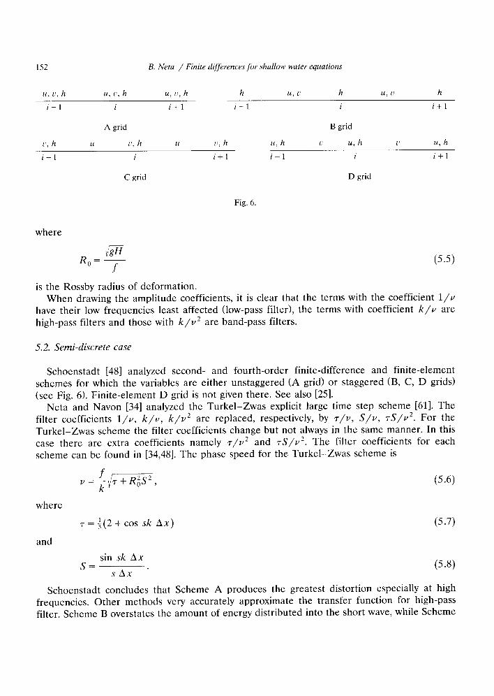
where
digH R,,= -
f is the Rossby radius of deformation.
When drawing the amplitude coefficients, it is clear that the terms with the coefficient l/v have their low frequencies least affected (low-pass filter), the terms with coefficient k/v are high-pass filters and those with k/v* are band-pass filters.
5.2. Semi-discrete case
Schoenstadt [48] analyzed second- and fourth-order finite-difference and finite-element schemes for which the variables are either unstaggered (A grid) or staggered (B, C, D grids) (see Fig. 6). Finite-element D grid is not given there. See also [25].
Neta and Navon [34] analyzed the Turkel-Zwas explicit large time step scheme [61]. The filter coefficients l/v, k/v, k/v2 are replaced, respectively, by r/v, S/v, Q-S/V*. For the Turkel-Zwas scheme the filter coefficients change but not always in the same manner. In this case there are extra coefficients namely r/v* and rS/v2. The filter coefficients for each
scheme can be found in [34,48]. The phase speed for the Turkel-Zwas scheme is
(W
where
T = +(2 + cos sk AX) (5.7)
and
sin sk Ax s=
SAX ’ (5 4
Schoenstadt concludes that Scheme A produces the greatest distortion especially at high frequencies. Other methods very accurately approximate the transfer function for high-pass filter. Scheme B overstates the amount of energy distributed into the short wave, while Scheme
B. Neta / Finite differences for shallow water equations 153
u,v,h u,v,h h
UP’ I,h
1
1
u,v,h h Fig. 7(a). Grid A.
h
L n
Fig. 7(b). Grid B.
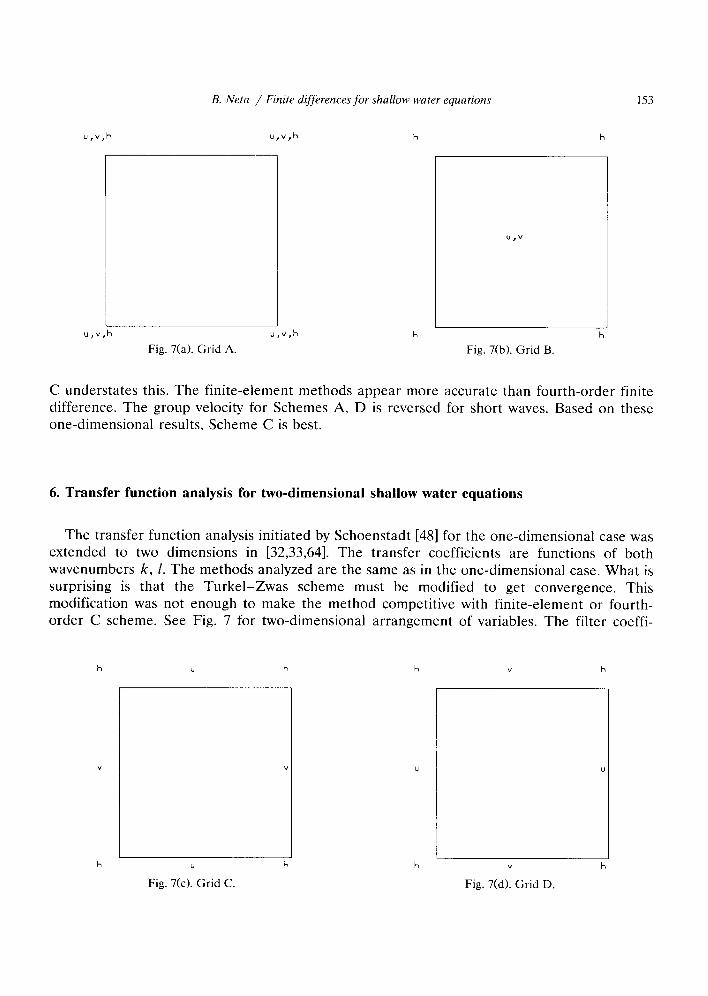
C understates this. The finite-element methods appear more accurate than fourth-order difference. The group velocity for Schemes A, D is reversed for short waves. Based on one-dimensional results. Scheme C is best.
finite these
6. Transfer function analysis for two-dimensional shallow water equations
The transfer function analysis initiated by Schoenstadt [48] for the one-dimensional case was extended to two dimensions in [32,33,64]. The transfer coefficients are functions of both wavenumbers k, 1. The methods analyzed are the same as in the one-dimensional case. What is surprising is that the Turkel-Zwas scheme must be modified to get convergence. This modification was not enough to make the method competitive with finite-element or fourth- order C scheme. See Fig. 7 for two-dimensional arrangement of variables. The filter coeffi-
h ” h h ” h
” n
”
h ”
Fig. 7(c). Grid C. Fig. 7(d). Grid D.
154
Table 5
B. Neta / Finite differences for shallow water equations
Scheme CY, ff> ,B(k, 1)
A2
B2
c2
D2
A4
B4
c4
D4
TZ
FET
FER
1 1
1 1
1 cos ;kd cos $ld
1 cos ;kd cos +ld
1 1
1 1
1 cos ;kd cos +ld
1 cm ;kd cos +ld
1 34 + cos ksd + cos lsd)
+(3 + cos kd + 2 cos ;kd cos Id) ;(3 + cos kd + 2 cos ;kd cos Id)
$(2+cos kd)(2+cos Id) ;(2+cos kd)(2+cos Id)
sin kd
d sin ;kd Icos ;ld
pi
sin +kd
id
sin kd pcos ;ld
d 8 sin kd -sin 2kd
6d -sin :kd + 27 sin tkd
12d cos i/d
- sin $kd + 27 sin +kd
12d 8 sin kd - sin 2kd
6d cos ;ld
sin ksd
sd 2( sin kd + sin ikd cos ld)
3d sin kd
+(2+cos IdId
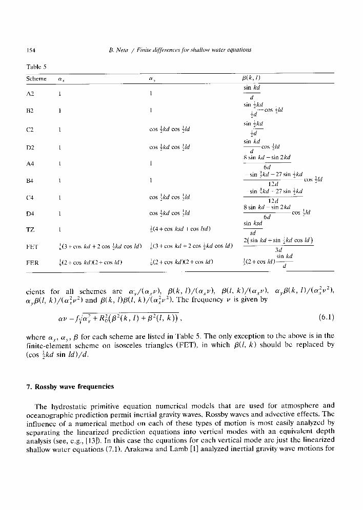
cients for all schemes are a,/(a,v>, P(k, I>/(a,v), P(l, k)/(a,v), a,P(k, l)/(azv2), c~,p(l, ~)/((Y:v~> and P(k, OpU; k)/(azv21. The frequency 1, is given by
cfv =f a; +RlQ2(k, 1) +p’(A k)) 7
where ayx, (Y,,, p for each scheme are listed in Table 5. The only finite-element scheme on isosceles triangles (FET), in which (cos ikd sin Zd)/d.
(6.1)
exception to the above is in the P(E, k) should be replaced by
7. Rossby wave frequencies
The hydrostatic primitive equation numerical models that are used for atmosphere and oceanographic prediction permit inertial gravity waves, Rossby waves and advective effects. The influence of a numerical method on each of these types of motion is most easily analyzed by separating the linearized prediction equations into vertical modes with an equivalent depth analysis (see, e.g., [13]). In this case the equations for each vertical mode are just the linearized shallow water equations (7.1). Arakawa and Lamb [l] analyzed inertial gravity wave motions for
B. Neta / Finite differences far shallow water equations 155
grids A, B, C, D. They found that the geostrophic adjustment for grids A, D is poor and that the adjustment for grids B, C is good.
In this section we discuss the treatment of Rossby waves in vorticity-divergence shallow water formulations with various finite-element and finite-difference schemes. For comparison the finite-difference primitive equations solution for grids A, B and C are also included (see
B',641).
7.1. Primitiue form
The linearized shallow water equations on a beta plane can be written as follows:
&A
z -fi; +gg
al! ah ; +“b+g-
ay
= 0,
= 0,
au
-1 =o.
dY
The frequency can be obtained by
PO* WF= -
6+E+(YK2’
where (Y, $I, 6, E depend on the method used and where PO These parameters are listed in [38] and reproduced in Table 6.
7.2. Vorticity-diuergence form
(7.1)
(7.2)
(7.3)
(7.4)
is an average value of df/dy.
The vorticity-divergence equation set, which is obtained by differentiating (7.1) and (7.2) with respect to x and y, respectively, and combining, can be written
z +fD + pc = 0, (7.5)
aD dl-f~+Su+y~$+~)=o. (7.6)
; +HD=O. (7.7)
156 B. Neta / Finite differences for shallow water equations
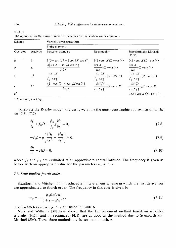
Table 6 The operators for the various numerical schemes for the shallow water equations
Scheme Vorticity-divergence form
Operator
Finite elements
Analytic Isosceles triangles Rectangular Staniforth and Mitchell
t55,561
a 1 i(3+cos x* +2cos txcos Y) $(2+cos xx2+cos Y) ;(2+cos X)(2+cos Y)
2(sin X+sin +Xcos Y) sin X z $(2 + cos Y)
sin X 9 P
3Ax -&2+cos Y)
6 P2 sin*fX
(; Ax)*
sinZLX (t A;)2 $(2+cos Y)
sin’+X ---+5+cos Y) (t Ax)
E
(Y’
k* (3+cosx-4cos~xcosY) sin’+Y
----+(2+cos X) sin’+Y
2 Ay* (:AY) ~$+cos X) (DAY)
$5 + cos X)(5 + cos Y)
*X=k Ax,Y=lAy.
To isolate the Rossby mode more easily we apply the quasi-geostrophic approximation to the set (7SH7.7)
ah z +HD=O,
(7.9)
(7.10)
where f,, and PO are evaluated at an approximate central latitude. The frequency is given as before with an appropriate value for the parameters IY, 9, 6, E.
7.3. Semi-implicit fourth order
Staniforth and Mitchell [56] introduced a finite-element scheme in which the first derivatives are approximated to fourth order. The frequency in this case is given by
(7.11)
The parameters LX, CX’, I/I, 6, E are listed in Table 6. Neta and Williams [38] have shown that the finite-element method based on isosceles
triangles (FET) and on rectangles (FER) are as good as the method due to Staniforth and Mitchell GM). These three methods are better than all others.
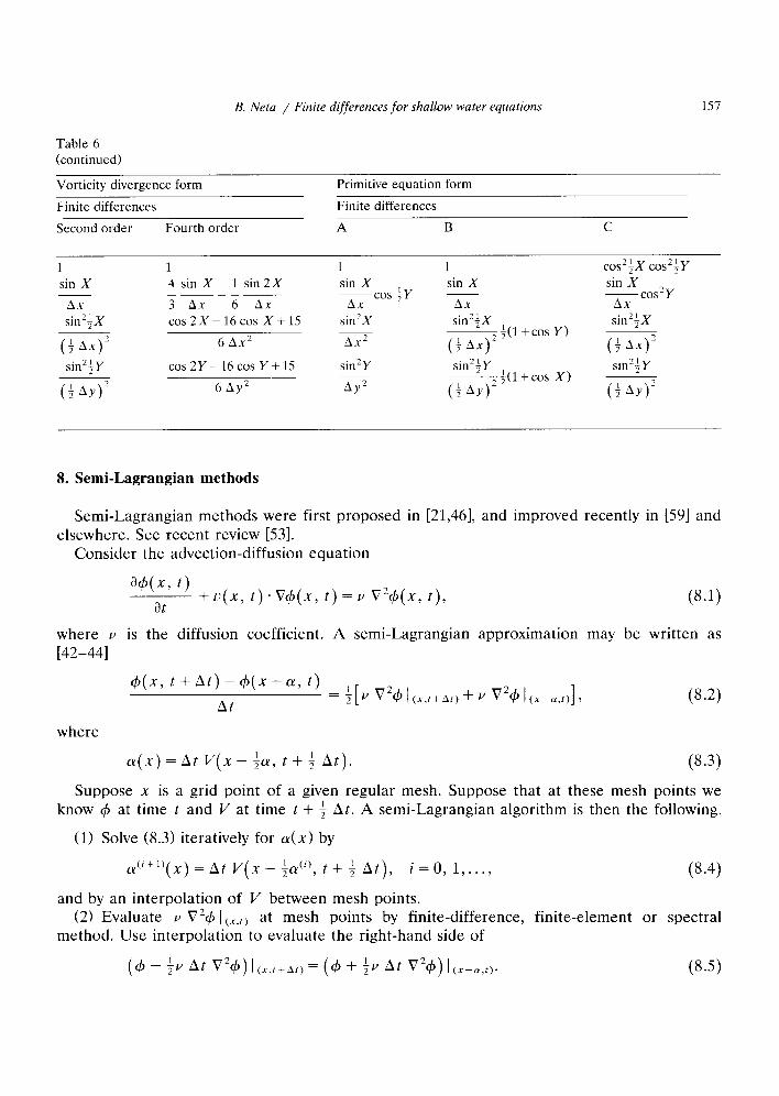
B. Neta / Finite differences for shallow water equations 157
Table 6 (continued)
Vorticity-divergence form
Finite differences
Second order Fourth order
Primitive equation form
Finite differences
A B C
1 1 1
sin X 4 sin X 1 sin 2X sin X __-
AX 3 Ax 6 Ax -cos $Y
AX
sin’+X cos2X-16cosX+15 sin2X
(4 Ax)~ 6 Ax’ AX2
1 cos2;x cos2;Y
sin X sin X - cos2Y
Ax Ax
sin’fX sin’;X ~;(l+cos Y) ~
(f Ax) (4 Ax)~
sin21Y * cos2Y-16cosY+15 sin2Y
(t AY)’ 6 Ay2 Ay2
sin2LY sin”+Y +$(l+cos x> ~
(t AY) (5 AY)*
8. Semi-Lagrangian methods
Semi-Lagrangian methods were first proposed in [21,46], and improved recently in [59] and elsewhere. See recent review [53].
Consider the advection-diffusion equation
a#+ t> at
+ u(x, t) +b(x, t) = v v2+, t),
where II is the diffusion coefficient. A semi-Lagrangian approximation may be written as [42-441
4(x, t + At) - 4(x -a, t) =I
At 2
where
1 (x,t+Ar) + v v24 1 (r-a~)] , (84
a(x) = At V(X - ;a, t + ; At). (84 Suppose x is a grid point of a given regular mesh. Suppose that at these mesh points we
know 4 at time t and V at time t + i At. A semi-Lagrangian algorithm is then the following.
(1) Solve (8.3) iteratively for a(x) by
aci+‘)(x) = At V(x - $zci), t + 3 At), i = 0, 1,. .., (8.4)
and by an interpolation of I/ between mesh points. (2) Evaluate v V*$J I cX,tj at mesh points by finite-difference, finite-element or spectral
method. Use interpolation to evaluate the right-hand side of
(4 - $’ At V’4) 1 (x,t+Af) = (4 + $’ At v’4) 1 (x-ay,t). (8.5)
158 B. Neta / Finite differences for shallow water equations
(3) Solve the above Helmholtz equation at mesh points (SOR, ADI, finite Fourier transform, finite elements).
(4) Repeat the steps to obtain 4(x, t + 2 At).
Remarks. (1) Eulerian schemes suffer from serious numerical dispersion and diffusion. (2) High-ord E 1 er u erian schemes tend to produce artificial extrema because of the unrealistic
phase speeds of the high wave number. (3) Lagrangian schemes suffer from distortion of the initial grid after a long integration
(more than twelve hours).
In two dimensions it is appropriate to consider the pseudo staggering suggested in [7]. “The scheme works well with the primitive form of the equations, uses unstaggered grid but does not propagate small scale energy in the wrong direction, works well with variable resolution and as computationally efficient as staggered formulation using the primitive form of the equations.”
9. Domain decomposition
One of the major developing areas in numerical analysis is parallel computation which offers the possibility of significantly faster computational speeds. Domain decomposition methods are based on subdivision of the domain into several (maybe overlapping) subdomains and solving the problem on several subdomains in parallel. The methods can be regarded as divide-and- conquer algorithms (see [65]). The interactions between the solutions on the subdomains lead to an iterative technique. When the number of subdomains is large, one can improve the convergence of this iterative procedure by using a coarse grid to obtain starting values of the solution on the interfaces. In this respect, the methods are similar to multigrid schemes. The crucial point is how to pass information from one domain to other processors. Two different approaches were followed in the literature. The first approach is based on decompositions of the domain into contiguous regions (see, e.g., [12] and references there). The second is based on having overlapping regions (Schwartz alternating method, see, e.g., [22-241 and references there).
The main difficulty of such parallel techniques is in the initial assignment of values to the interfaces between subdomains. The more accurate such values are, the faster the convergence. We have already mentioned the idea based on multigrid. There are several other possibilities to accelerate convergence (see the proceedings of four international conferences on domain decomposition [5,6,14,X]). According to Lions [24] the approach based on optima1 control as followed by Glowinski et al. [16,17] is a bit faster, at least for Laplace equations.
Neta and Okamoto 1351 have suggested an acceleration based on boundary elements. These two approaches for shallow water equations are now under investigation by Neta and Navon.
10. Conclusions
This paper reviewed analyses of finite-element and finite-difference schemes for the solution of the shallow water equations. The superiority of certain finite-element methods is indicated. Some recent results in parallel computations are included.
B. Neta / Finite differences for shallow water equations 159
References
[I] A. Arakawa and V.R. Lamb, Computational design of the basic dynamical processes of the UCLA General Circulation Model, in: Methods Comput. Phys. 17 (Academic Press, New York, 1977) 173-265.
[2] W. Blumen, Geostrophic adjustment, Reu. Geophys. Space Phys. 10 (1972) 485-528. [3] A. Cahn, An investigation of the free oscillations of a simple current system, J. Meteorology 2 (1945) 113-119. [4] M.M. Cecchi, Domain decomposition method for shallow water flow problems, in: H. Niki and M. Kawahara,
eds., Proc. Internat. Conf on Computational Methods in Flow Analysis (Okayama Univ. of Science, Japan, 1988)
1322-1329. [5] T.F. Chan, R. Glowinski, J. Periaux and O.B. Widlund, eds., Proc. 2nd Internat. Syrnp. on Domain Decomposi-
tion Methods (SIAM, Philadelphia, PA, 1989). [6] T.F. Chan, R. Glowinski, J. Periaux and O.B. Widlund, eds., Proc. 3rd Internat. Symp. on Domain Decomposi-
tion Methods for PDEs (SIAM, Philadelphia, PA, 1989). [7] J. Cot& S. Gravel and A. Staniforth, Improving variable-resolution finite-element semi-Lagrangian integration
schemes by pseudo-staggering, Monthly Weather Reo. 118 (1990) 2718-2731. [8] J. C8tC and A. Staniforth, A two-time-level semi-Lagrangian semi-implicit scheme for spectral models, Monthly
Weather Ret,. 116 (1988) 2003-2012. [9] M.P.J. Cullen and C.D. Hall, Forecasting and general circulation results from finite element models, Quart. .I.
Roy. Meteorological Sot. 105 (1979) 571-592. [lo] C.A.J. Fletcher, Computational Galerkin Methods (Springer, New York, 1984). [ 1 l] M.G.G. Foreman, A two dimensional dispersion analysis of selected methods for solving the linearized shallow
water equations, J. Comput. Phys. 56 (1984) 287-323. [12] D. Funaro, Multidomain spectral approximation of elliptic equations, Numer. Methods Partial Differential
Equations 2 (1986) 187-205. [13] A.E. Gill, Atmosphere-Ocean Dynamics (Academic Press, New York, 1982). [14] R. Glowinski, G.H. Golub, G.A. Meurant and J. Periaux, eds., Proc. 1st Internat. Symp. on Domain Decomposi-
tion Methods for Partial Differential Equations (SIAM, Philadelphia, PA, 1988). [15] R. Glowinski, Y.A. Kuznetsov, G. Meurant, J. Periaux and 0. Widlund, eds., Proc. 4th Internat. Symp. on
Domain Decomposition Methods for Partial Differential Equations (SIAM, Philadelphia, PA, to appear). [16] R. Glowinski and P. Le Tallec, Augmented Lagrangian interpretation of the nonoverlapping Schwarz alternat-
ing scheme, in: T.F. Chan et al., eds., Proc. 3rd Internat. Symp. on Domain Decomposition Methods for PDEs (SIAM, Philadelphia, PA, 1989) 224-231.
[17] R. Glowinski, Q.V. Dinh and J. Periaux, Domain decomposition methods for nonlinear problems in fluid dynamics, Comput. Methods Appl. Mech. Engrg. 40 (1) (1983) 27-109.
[18] G.J. Haltiner and R.T. Williams, Numerical Prediction and Dynamic Meteorology (Wiley, New York, 1980). [19] R.G. Kelley and R.T. Williams, A finite element prediction model with variable element sizes, Naval
Postgraduate School Report NPS-63 Wu76101, Monterey, CA, 1976. [20] I. Kinnmark, The Shallow- Water Wat,e Equations: Formulation, Analysis, and Application (Springer, Berlin,
1985). , [21] T.N. Krishnamurti, Numerical integration of primitive equations by a quasi-Lagrangian advective scheme, J.
Appl. Met. l(1962) 508-521. [22] P.L. Lions, On the Schwarz alternating method, in: R. Glowinski et al., eds., Proc. 1st Internat. Symp. on
Domain Decomposition Methods for Partial Diff erential Equations (SIAM, Philadelphia, PA, 1988) l-42. [23] P.L. Lions, On the Schwarz alternating method II: Stochastic interpretation and order properties, in: T.F. Chan
et al., eds., Proc. 2nd Internat. Symp. on Domain Decomposition Methods (SIAM, Philadelphia, PA 1989) 47-70. [24] P.L. Lions, On the Schwarz alternating method III: A variant for nonoverlapping subdomains, in: T.F. Chan et
al., eds., Proc. 3rd Internat. Symp. on Domain Decomposition Methods for PDEs (SIAM, Philadelphia, PA, 1989) 202-223.
[25] F. Mcsinger, Dependence of vorticity analogue and the Rossby wave phase speed on the choice of horizontal grid, Sci. Math. 10 (1979) 5-1.5.
[26] A.R. Mitchell and R. Wait, The Finite Element Method in Partial Diff erential Equations (Wiley, London, 1977). [27] K.B. Monk, Studies of baroclinic flow over topography using semi-Lagrangian, semi-implicit model, Dept.
Meteorology, Naval Postgraduate School, Monterey, CA, 1989.
160 B. Neta / Finite differences for shallow water equations
[28] I.M. Navon, A Numerov-Galerkin technique applied to a finite-element shallow-water equations model with exact conservation of integral constraints, in: T. Kawai, ed., Proc. 4th Internat. Symp. on Finite Element Methods in Flow Problems (Chuo Univ., Tokyo, 1982) 75-85.
[29] I.M. Navon, A Numerov-Galerkin technique applied to a finite element shallow-water equations model with enforced conservation of integral invariants and selective lumping, J. Comput. Phys. 52 (1983) 313-339.
[30] I.M. Navon, A review of finite-element methods for solving the shallow-water equations, Supercomputer Computations Research Institute Report FSU-SCRI-88-49, Tallahassee, FL, 1988.
[31] I.M. Navon and H.A. Riphagen, An implicit compact fourth-order algorithm for solving the shallow-water equations in conservation-law form, Monthly Weather Rec. 107 (1979) 1107-1127.
[32] B. Neta, Analysis of the Turkel-Zwas scheme for the shallow-water equations, in: W.F. Ames, ed., I&ICS Trans. on Scientific Computing ‘88, Vols. 1.1 and 1.2: Numerical and Applied Mathematics (Baltzer, 1989) 257-264.
[33] B. Neta and C.L. DeVito, The transfer function analysis of various schemes for the two dimensional shallow-water equations, Comput. Math. Appl. 16 (1988) 111-137.
1341 B. Neta and I.M. Navon, Analysis of the Turkel-Zwas scheme for the shallow-water equations, J. Comput. Phys. 80 (1989) 277-299.
[35] B. Neta and N. Okamoto, On domain decomposition methods for solving partial differential equations, Naval Postgraduate School Technical Report NPS-53-90-004, Monterey, CA, 1990.
[36] B. Neta and R.T. Williams, Stability and phase speed for various finite element formulations of the advection equation, Comput. & Fluids 14 (1986) 393-410.
[37] B. Neta and R.T. Williams, Finite elements versus finite differences for fluid flow problems, in: G.N. Pande and J. Middleton, eds., Proc. Internat. Conf on Numerical Methods in Engineering: Theory and Applications, II (Martinus Nijhoff, Dordrecht, 1987) Tll/l-8.
[38] B. Neta and R.T. Williams, Analysis of finite element methods for the solution of the vorticity-divergence form of the shallow water equations, in: M. Yasuhara, H. Daiguji and K. Oshima, eds., Numerical Methods in Fluid Dynamics I, Proc. Internat. Symp. Comp. Fluid Dynamics (Nagoya, 1989) 402-407.
[39] B. Neta, R.T. Williams and D.E. Hinsman, Studies in a shallow water fluid model with topography, in: R. Vichnevetsky and J. Vignes, eds., Numerical Mathematics and Applications (Elsevier, Amsterdam, 1986) 347-354.
[40] A.M. Obukhov, Izc. Akad. Nauk SSR Ser. Geograph.-Geofiz. 13 (4) (1949) 281. [41] J. Pedlosky, Geophysical Fluid Dynamics (Springer, New York, 2nd ed., 1987). [42] J. Pudykiewicz and A. Staniforth, Some properties and comparative performance of the semi-Lagrangian
method of Robert in the solution of the advection-diffusion equation, Atmosphere-Ocean 22 (3) (1984) 283-308.
[43] A. Robert, A stable numerical integration scheme for the primitive meteorological equations, Atmosphere-Oc- ean 19 (1981) 35-46.
[44] A. Robert, A semi-Lagrangian and semi-implicit numerical integration scheme for the primitive meteorological equations, J. Meteorological Sot. Japan 60 (1982) 319-324.
[45] C.G. Rossby, On the mutual adjustment of pressure and velocity distributions in certain simple current systems, J. Marine Research 1 (1937-1938) 15-28; 239-263.
[46] J.S. Sawyer, A semi-Lagrangian method of solving the vorticity advection equations, Tellus 15 (1963) 336-342. [47] A.L. Schoenstadt, The effect of spatial discretization on the steady-state and transient behavior of a dispersive
wave equation, J. Comput. Phys. 23 (1977) 364-379. [48] A.L. Schoenstadt, A transfer function analysis of numerical schemes used to simulate geostrophic adjustment,
Monthly Weather Rec. 108 (1980) 1248-1259. [49] H.A. Schwarz, Gesammelte Mathematische Abhandlungen 2 (Springer, Berlin, 1890) 133-134. [50] G. Sewell, Analysis of a Finite Element Method, PDE/Protran (Springer, New York, 1985). [51] A.N. Staniforth, The application of the finite-element method to meteorological simulations - a review,
Internat. J. Numer. Methods Fluids 4 (1984) 1-12. [.52] A.N. Staniforth, Review: formulating efficient finite-element codes for flows in regular domains, Internat. J.
Numer. Methods Fluids 7 (1987) 1-16. [53] A.N. Staniforth and J. Cot& Semi-Lagrangian integration schemes for atmospheric models - a review, Monthly
Weather Rec. 119 (1991) 2206-2223.
B. Neta / Finite differences for shallow water equations 161
[54] A.N. Staniforth and R.W. Daley, A baroclinic finite-element model for regional forecasting with the primitive equations, Monthly Weather Reu. 107 (1979) 107-121.
[55] A.N. Staniforth and H.L. Mitchell, A semi-implicit finite-element barotropic model, Monthly Weather Rec. 105 (1977) 154-169.
[56] A.N. Staniforth and H.L. Mitchell, A variable resolution finite-element technique for regional forecasting with the primitive equations, Monthly Weather Rea. 106 (1978) 439-447.
[57] G. Strang and G.J. Fix, An Analysis of the Finite Element Method (Prentice-Hall, Englewood Cliffs, NJ, 1973). [58] F.G. Stremler, Introduction to Communication Systems (Addison-Wesley, Reading, MA, 1977). [59] C. Temperton and A.N. Staniforth, An efficient two-time-level semi-Lagrangian semi-implicit integration
scheme, Quart. J. Roy. Meteorological Sot. 113 (1987) 1025-1039. [60] V. Thomee and B. Wendroff, Convergence estimates for Galerkin methods for variable coefficient initial value
problems, SLAM J. Numer. Anal. 11 (1974) 1059-1068. [61] E. Turkel and G. Zwas, Explicit large time step schemes for the shallow-water equations, in: R. Vichnevetsky
and R.S. Stepleman, eds., Advances in Computer Methods for Partial Differential Equations (IMACS, New Brunswick, NJ, 1979) 65-69.
[62] R. Vichnevetsky and J.B. Bowles, Fourier Analysis of Numerical Approximations of Hyperbolic Equations, SIAM Stud. Appl. Math. (SIAM, Philadelphia, PA, 1982).
[63] R. Vichnevetsky and B. Peiffer, Error waves in finite-elements and finite-difference methods for hyperbolic equations, in: R. Vichnevetsky, ed., Advances in Computer Methods for Partial Differential Equations (AICA, Rutgers Univ., New Brunswick, NJ, 1975).
[64] R.C. Wajsowicz, Free planetary waves in finite-difference numerical model, J. Phys. Oceanography 16 (1986) 773-789.
[65] O.B. Widlund, Domain decomposition algorithms and the bicentennial of the French revolution, SIAM News 22 (1989) 20.
[66] R.T. Williams, On the formulation of finite-element prediction models, Monthly Weather Reo. 109 (1981) 463-466.
[67] R.T. Williams and A.L. Schoenstadt, Formulation of efficient finite clement prediction models, Naval Postgrad- uate School Report NPS-63-80-011, Monterey, CA, 1980.
[68] R.T. Williams and O.C. Zienkiewicz, Improved finite-element forms for the shallow-water equations, Internat. J. Numer. Methods Fluids 1 (1981) 81-97.
[69] F. Winninghoff, On the adjustment toward a geostrophic balance in a simple primitive equation model with application to the problem of initialization and objective analysis, Ph.D. dissertation, Univ. California, Los Angeles. 1968.
1701 O.C. Zienkiewicz, The Finite Element Methods in Engineering Science (McGraw-Hill, New York, 1977).