isoparametric finite elements - petra christian...

Isoparametric

Finite Elements

Wong Foek Tjong, Ph.D.

Petra Christian University

Surabaya

General Lecture in Magister Teknik Sipil

Universitas Diponegoro, 1 Feb 2014

2 2014/2/12

Lecture Outline

1. Overview of the FEM

2. Governing equations of plane-strain/plane-stress problems

3. Finite element formulation

4. Isoparametric elements

5. Element tests and applications

6. References

3 2014/2/12

Behavior of a

Real Structure

Experiment

Replicate conditions of the

structure (possibly on a

smaller scale) and observe

the behavior of the model

Simulation

Simplifications and

assumptions of the

real structure

Mathematical

Model Physical

Model

4 2014/2/12

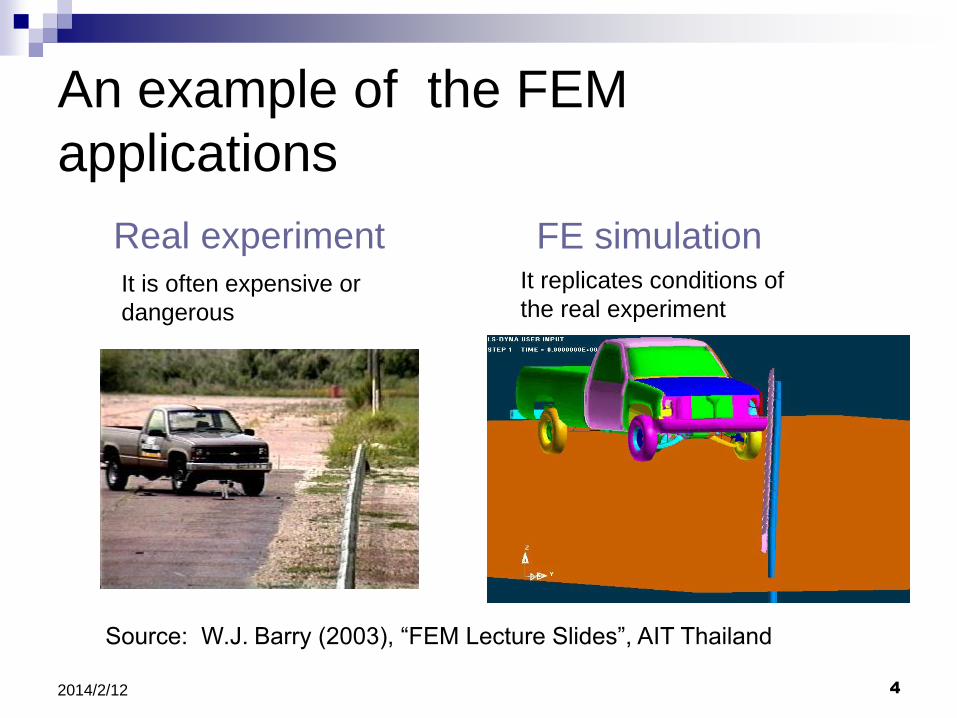
An example of the FEM

applications

Real experiment FE simulation It is often expensive or

dangerous

It replicates conditions of

the real experiment

Source: W.J. Barry (2003), “FEM Lecture Slides”, AIT Thailand

5 2014/2/12

The need for modeling

A real structure cannot be analyzed, it can only be “load tested” to determine the responses

We can only analyze a “model” of the structure (perform simulation)

We need to model the structure as close as possible to represent the behavior of the real structure

Source: W. Kanok-Nukulchai

6 2014/2/12

Mathematical

Models

Analytical Solution

Techniques

Numerical Solution

Techniques

Closed-form

Solutions

Only possible for

simple geometries and

boundary conditions

•Finite difference methods

•Finite element methods

•Boundary element methods

•Mesh-free methods

•etc.

7 2014/2/12

It is a computational technique used to obtain approximate solutions of engineering problems.

The results are generally not exact.

However, the accuracy of the results can be improved either using finer mesh (h-refinement) or higher degree elements (p-refinement)

What is FEM?

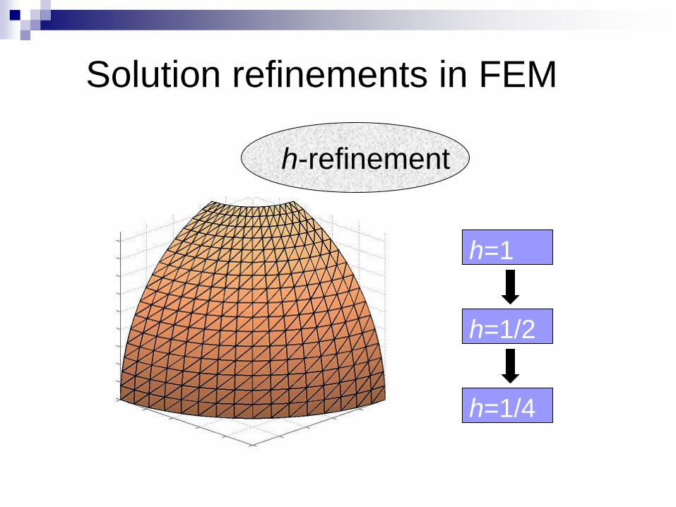
Solution refinements in FEM

h-refinement

h=1/4

h=1/2

h=1

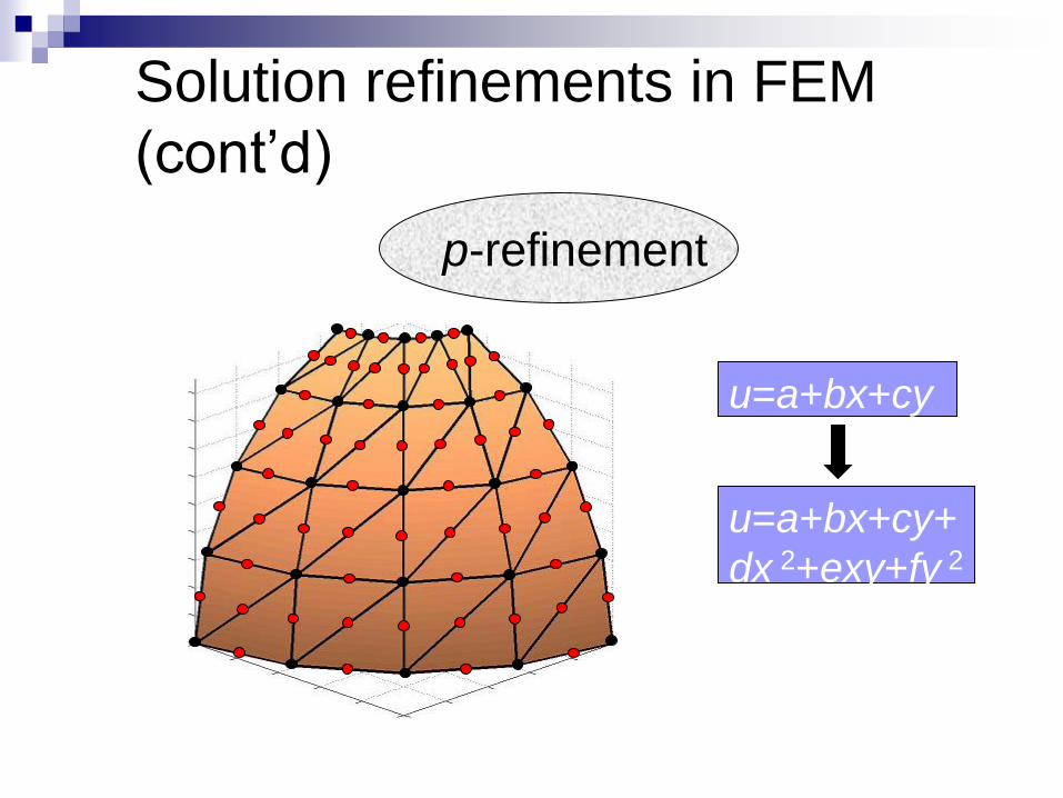
Solution refinements in FEM

(cont‟d)

p-refinement

h=1 h=1/2 u=a+bx+cy+

dx 2+exy+fy 2

u=a+bx+cy

10 2014/2/12

For General purposes:

NASTRAN, ANSYS, ADINA, ABAQUS, etc.

For structural analysis, particularly in Civil Engineering:

SANS, SAP, STAAD, GT STRUDL, MIDAS, DIANA, STRAND 7, etc.

For building structures:

ETABS, BATS etc.

Examples of FEM software

11 2014/2/12

FEM is originated as a method of structural analysis but is now widely used in various disciplines such as heat transfer, fluid flow, seepage, electricity and magnetism, and others.

The present discussion will focus on FEM for structural analysis, with the scope: Plane stress/plane strain problems

Linear static analysis

Isoparametric formulation Bilinear isoparametric quadrilateral element (Q4)

Focus of lecture

12 2014/2/12

Lecture Outline






6. References

Plane stress

A stress condition that prevails in a thin plate loaded only in its own plane, say xy plane, and without restraint in its perpendicular direction.

ζz=ηyz= ηzx=0

Typical examples are thin plates loaded in the plane of the plate.

x, u

y, v z, w

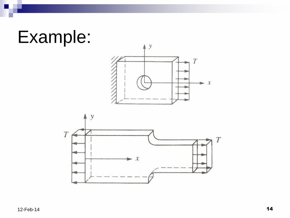
Example:

14 12-Feb-14

Plane strain

A deformation state in which w=0 everywhere

u=u(x, y)

v=v(x, y)

Thus, εz=γxz= γyz=0

A state of strain in which the strain normal to the x-y plane and the shearing strains γxz and γyz are zero.

x , u

y , v

z , w

One unit

length

O

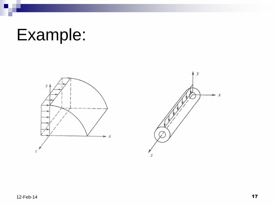
Plane strain (cont‟d)

The plane strain model is realistic for a long body with constant cross section subjected to planar loads that do not vary along the body.

Examples: A slice of an underground

tunnel that lies along z axis

A slice of an earth retaining wall

Only a unit thickness of the body is considered in an analysis using the plain strain model.

x , u

y , v

z , w

One unit

length

O

Example:

17 12-Feb-14

Basic concepts from the theory of

elasticity Consider a plane stress/strain

model of a body (structure) as

illustrated here.

The body is subjected to:

Concentrated force P

Distributed surface forces p1 and

p2, can be given in the unit of

[force]/[area] or [force]/[length]

Body force b=b(x,y), e.g. due to

the self-weight of the body,

[force]/[volume]

Temperature change T 0C

x , u

y , v

O

P

p2=p(y)

p1=p(x)

Note that a force is a vector,

while temperature is a scalar.

The plane stress/strain problem is: given the external loads, temperature change, and displacement boundary condition, find the displacement field, the strain field and the stress field.

19 12-Feb-14

x , u

y , v

O

P

p2=p(y)

p1=p(x)

The results of an analysis are:

Two displacement components, i.e. u and v

Three strain components, i.e. εx , εy , γxy

Three stress components, i.e. ζx , ζy , ηxy

In most FE softwares we can express the

stress results in terms of:

Principal stresses

von Mises stress

20 12-Feb-14

Output of an analysis

Governing equations

Three basic set of equations in the theory of elasticity are:

Strain-displacement equations

Stress-strain equations

Equations of equilibrium

21 12-Feb-14

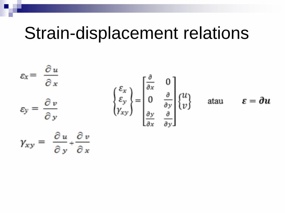
Strain-displacement relations

Stress-strain relations

Plane stress

For a body made up from isotropic materials, the

stress-strain relation is

Notice that the strain in z direction may not be zero

2

12

1 0 1

1 0 11 1

0 0 (1 ) 0

x x

y y

xy xy

E E T

( )z x y TE

Stress-strain relations (cont‟d)

Plane strain

For a body made up from isotropic materials, the

stress-strain relation is

Notice that stress ζz may not be zero

( )z x y E T

12

1 0 1

1 0 1(1 )(1 2 ) 1 2

0 0 (1 2 ) 0

x x

y y

xy xy

E E T

The Ord River Dam. Source:

www.australiaadventures.com

Equations of equilibrium

0yxx

xbx y

0xy y

ybx y

Given geometrical and material properties and external actions P, p, b, T, and support displacement u0, find u(x,y) that satisfies:

Strain-displacement equations: 𝛆 = 𝛛𝐮

Stress-strain equations: 𝛔 = 𝐄(𝛆 − 𝛆𝟎)

Equations of equilibrium: 𝛛𝐓𝛔 + 𝐛 = 𝟎

on the whole body and satisfies the given boundary conditions.

26 12-Feb-14

Strong form problem statement

The principle of virtual work

The FEM does not directly use the strong

form of governing equations, instead it

uses the weak form of the equations.

obtained from the principle of virtual work.

The weak form can be obtanied using:

The principle of stationary potential energy


27 12-Feb-14

28

x , u

y , v

O

P

p2=p(y)

p1=p(x)

(xP, yP)

S1: the surface on which p1 acts

S2: the surface on which p2 acts

𝛿𝑈 = 𝛿𝑊

29 12-Feb-14

x , u

y , v

O

P

p2=p(y)

p1=p(x)

(xP, yP)

Weak form problem statement

Given geometrical and material properties and

external actions P, p, b, T, and support

displacement u0, find u(x,y) such that for all

admissible δu

𝛿𝛆T𝛔 𝑑𝑉𝑉

= 𝛿𝐮T𝐏 𝑥P, 𝑦P + 𝛿𝐮T𝐩 𝑑𝑆

𝑆

+ 𝛿𝐮T𝐛 𝑑𝑉𝑉

where σ is defined in terms of u using the strain-

displacement and stress-strain relations

30 12-Feb-14

31 2014/2/12

Lecture Outline






6. References

32 2014/2/12

Lecture Outline






6. References

33 2014/2/12

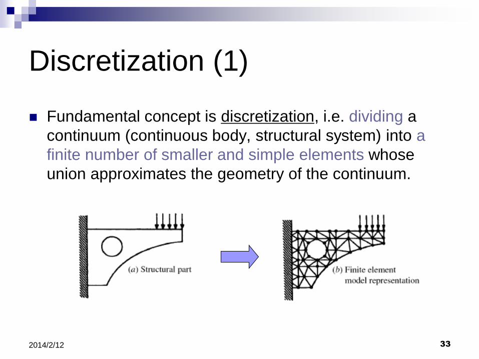
Fundamental concept is discretization, i.e. dividing a

continuum (continuous body, structural system) into a

finite number of smaller and simple elements whose

union approximates the geometry of the continuum.

Discretization (1)

Source: http://members.ozemail.com.au/~comecau/autostep.htm

Discretization (2)

Element formulation

In FE formulation, we need to formulate an

element to obtain the element stifness

equation

𝐤𝐝 = 𝐟

Once we have this equation, the solution

for the whole structure can be obtained

using the direct stiffness method.

35 12-Feb-14

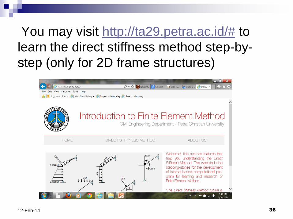
You may visit http://ta29.petra.ac.id/# to

learn the direct stiffness method step-by-

step (only for 2D frame structures)

36 12-Feb-14

http://ta29.petra.ac.id/



Consider a quadrilateral element of the

thickness h as illustrated here

The displacement field within the element:

𝐮 =𝑢𝑣=𝑢(𝑥, 𝑦)𝑣(𝑥, 𝑦)

37 12-Feb-14

1

2

3

4

u1

v1

u2

u3

u4

v2

v3 v4

x, u

y, v

o

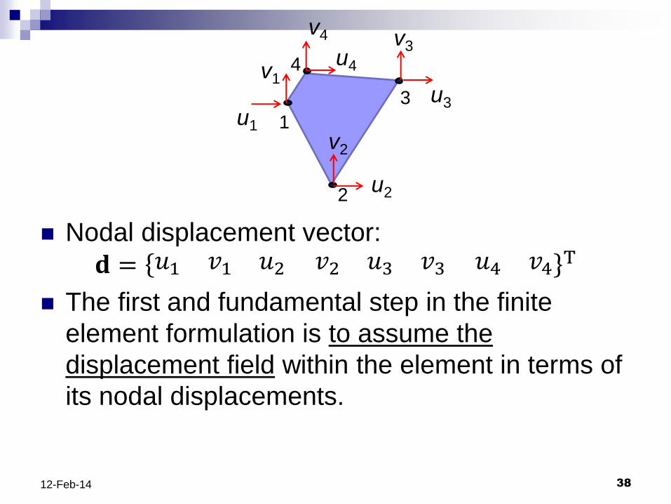
Nodal displacement vector:

𝐝 = 𝑢1 𝑣1 𝑢2 𝑣2 𝑢3 𝑣3 𝑢4 𝑣4 T

The first and fundamental step in the finite

element formulation is to assume the

displacement field within the element in terms of

its nodal displacements.

38 12-Feb-14

1

2

3

4

u1

v1

u2

u3

u4

v2

v3 v4

The assumed displacement field within the

element can be expressed as:

𝑢 = 𝑁𝑖𝑢𝑖4

𝑖<1

𝑣 = 𝑁𝑖𝑣𝑖4

𝑖<1

Or written in matrix form:

𝐮 = 𝐍𝐝

where

𝐍 =𝑁1 0 𝑁20 𝑁1 0

0 𝑁3 0

𝑁2 0 𝑁3 𝑁4 0

0 𝑁4

40

𝐮 = 𝐍𝐝

N is the matrix of shape functions

N is also called the matrix of interpolation

functions, because it interpolates the

displacement field u=u(x, y) from the nodal

displacements

Interpolation

function

41 12-Feb-14

Strain-displacement relationships

Thus we can write

where

Matrix B gives strains at any point within the element

due to unit values of nodal displacements.

Matrix of differential

operators

3x2 2x8 3x8

𝛆 = 𝛛𝐮

𝛆 = 𝛛𝐍𝐝

𝛆 = 𝐁𝐝

𝐁 = 𝛛𝐍

Stress-strain relationships (without considering temperature effect)

thus


where

δUe : the virtual strain energy of internal stresses

δWe : the virtual work of external forces on the elements

𝛔 = 𝐄𝛆

𝛔 = 𝐄 𝐁 𝐝

𝜹𝑼e = 𝜹𝑾e

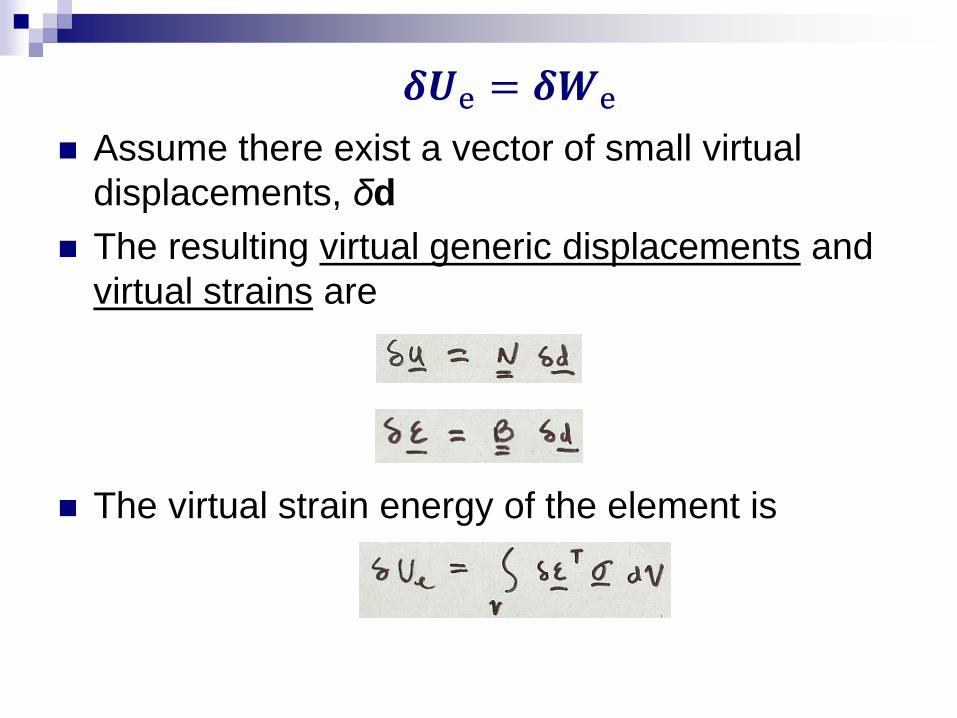
Assume there exist a vector of small virtual

displacements, δd

The resulting virtual generic displacements and

virtual strains are

The virtual strain energy of the element is

𝜹𝑼e = 𝜹𝑾e

The external virtual work of nodal and body

forces are

(1)

(2)

Substituting the eqs. (1) and (2) into

and cancelling δdT form both sides of the eq.

result in

Thus, the element stiffness matrix is

The equivalent nodal load vector due to body

forces is

Let us rename the actual nodal force vector

47 2014/2/12

Lecture Outline




4. Isoparametric elements Bilinear isoparametric quadrilateral

element


6. References

Q4 Isoparametric Element

Consider the quadrilateral element

We need to obtain the expression for the shape

functions N1,..., N4

48 12-Feb-14

1

2

3

4

u1

v1

u2

u3

u4

v2

v3 v4

x, u

y, v

o

If we formulate the quadrilateral element

directly in the cartesian coordinate system,

we will face technical difficuties:

The expression for the shape functions is

complicated

It is difficult to evaluate the integration in the

stiffness matrix and equivalent nodal force

vectors expressions exactly

49 12-Feb-14

To overcome the difficulties and moreover,

to facilitates the use of elements with

curved edges, we map the element onto a

square element defined in natural (ξ, η)

coordinates.

The square element is called parent or master

element.

50 12-Feb-14

To introduce the isoparametric concept,

we will consider a type of quadrilateral

element with four nodes for analysis of

plane stress/plane strain problems.

This element is the standard “plane

bilinear isoparametric element” (Q4).

51 12-Feb-14

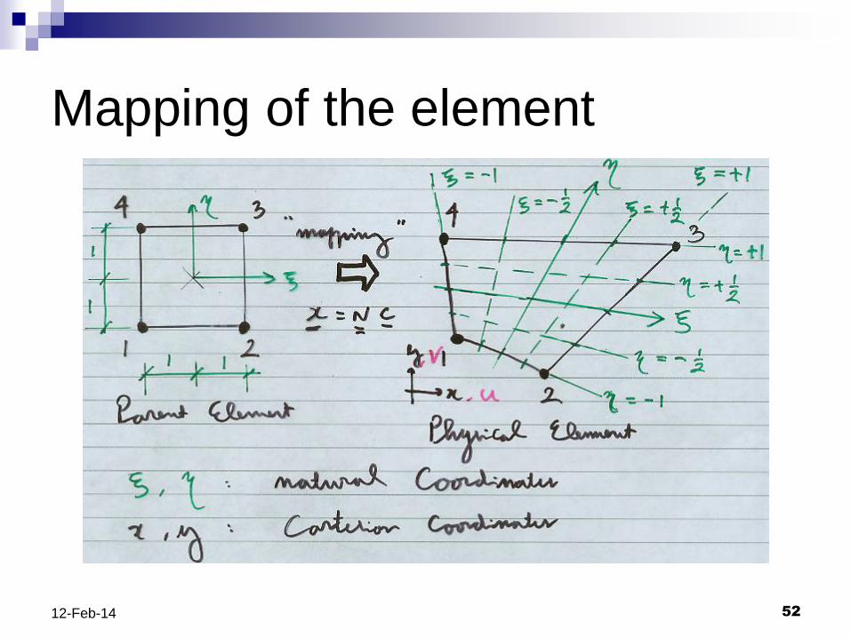
Mapping of the element

52 12-Feb-14

The geometry of the quadrilateral element is

described by:

53 12-Feb-14

𝑥 = 𝑁𝑖𝑥𝑖4

𝑖<1; 𝑦 = 𝑁𝑖𝑦𝑖

4

𝑖<1

Nodal coordinates:

1 𝑥1, 𝑦1

2 𝑥2, 𝑦2

3 (𝑥3, 𝑦3) 4 (𝑥4, 𝑦4)

Or, written in matrix form:

𝐱 = 𝐍𝐜

where

𝐍 =𝑁1 0 𝑁20 𝑁1 0

0 𝑁3 0

𝑁2 0 𝑁3 𝑁4 0

0 𝑁4

and

𝐜 = 𝑥1 𝑦1 𝑥2 𝑦2 𝑥3 𝑦3 𝑥4 𝑦4 T

54 12-Feb-14

The shape functions are functions of

natural coordinates ξ and η.

55 12-Feb-14

(ξ, η)=(0, 0) is the center of the element

u=Nd

x=Nc

The element is called bi-linear because

the shape functions Ni are linear in ξ and

linear in η.

It is called isoparametric because the

shape functions for interpolation of the

geometry are the same as those for

interpolation of the displacement field.

56 12-Feb-14

Displacement interpolation

Geometry interpolation

The strain vector is

The math difficulty here is that we have to

diffentiate u and v with respect to x and y,

but u and v are functions of ξ and η.

57 12-Feb-14

To overcome the difficulty, we apply the

chain rule for partial differentiation

Then,

58 12-Feb-14

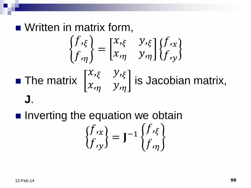
Written in matrix form, 𝑓,𝜉𝑓,𝜂=𝑥,𝜉 𝑦,𝜉𝑥,𝜂 𝑦,𝜂

𝑓,𝑥𝑓,𝑦

The matrix 𝑥,𝜉 𝑦,𝜉𝑥,𝜂 𝑦,𝜂

is Jacobian matrix,

J.

Inverting the equation we obtain

𝑓,𝑥𝑓,𝑦= 𝐉;1

𝑓,𝜉𝑓,𝜂

59 12-Feb-14

Let define Γ as the inverse of the Jacobian

matrix

Thus the derivatives of u and v can be

written as

60 12-Feb-14

61 12-Feb-14

d

62 12-Feb-14

Since ε=Bd, it can be concluded that the

strain-displacement matrix is

63 12-Feb-14

The derivatives of the shape functions

Is B a polynomial function?

64 12-Feb-14

The Jacobian matrix for the bilinear

element can be written as

65 12-Feb-14

The element stiffness matrix is

𝐤 = 𝐁T𝐄𝐁 𝑑𝑉𝑉

= ℎ 𝐁T𝐄𝐁 𝑑𝐴𝐴

The integration can be carried out in the

isoparametric space, over the parent

element, efficiently and accurately.

To illustrate the integration, tet consider

the computation of the area of an element

66 12-Feb-14

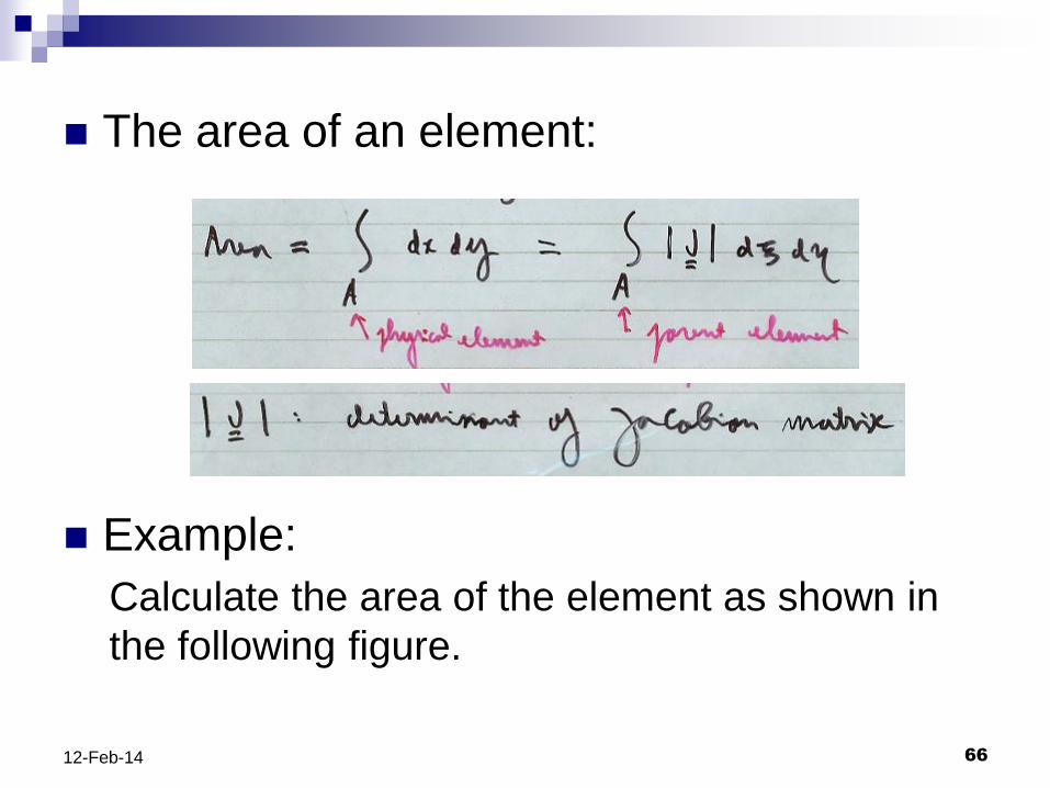
The area of an element:

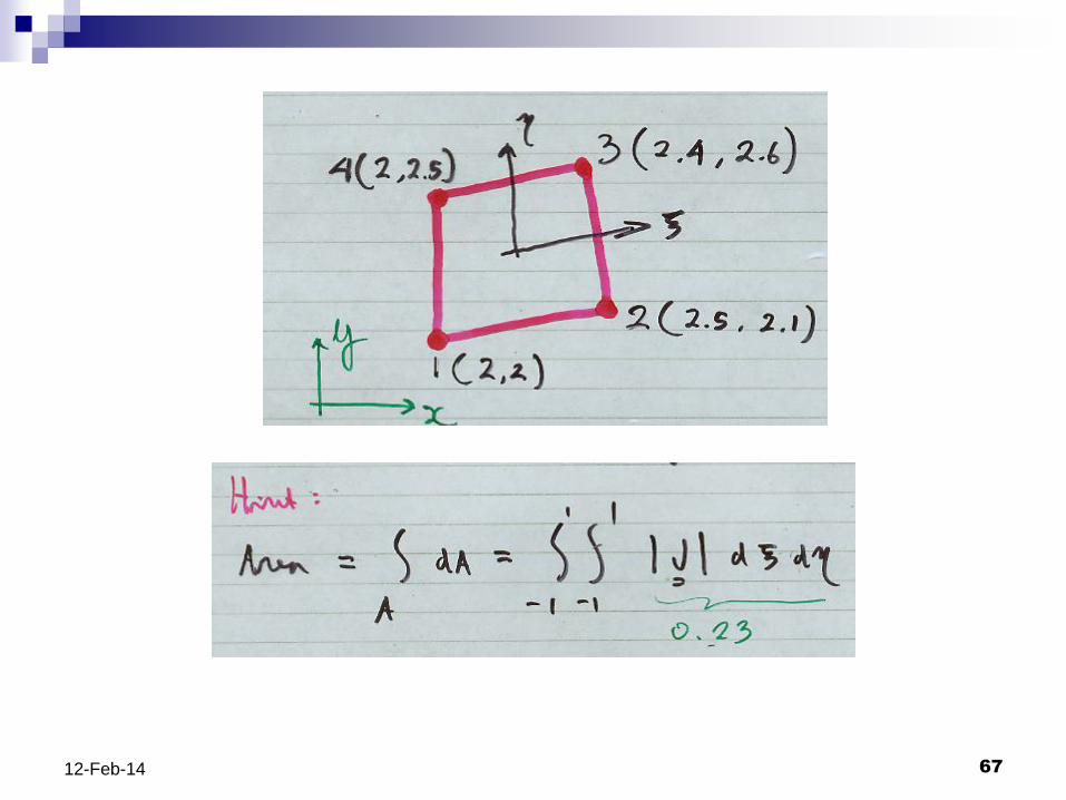
Example:

Calculate the area of the element as shown in

the following figure.

67 12-Feb-14

68 12-Feb-14

Equivalent nodal loads

69 12-Feb-14

Practical formulas for evaluating

equivalent nodal loads

70 12-Feb-14

71 12-Feb-14

Gauss Quadrature

Quadrature: evaluating an integral

numerically

For 1D integration:

First, transform from arbitrary integration limits

to −1 to +1

72 12-Feb-14

The transformation (mapping) is given by

Thus,

Here 𝜙(𝜉) incorporates the Jacobian of the

transformation,

𝐽 =𝑑𝑥

𝑑𝜉

73 12-Feb-14

Then evaluate the integral as follows,

A n-point Gauss qaudrature can integrate

exactly a polynomial of degree 2n-1

For a nonpolynomial function, the result will

not be exact-- the higher the number of

sampling points, the better the accuracy of the

result.

74 12-Feb-14

75 12-Feb-14

Examples:

Using two sampling point, we can

This intergral cannot be exaclty evaluated:

1

2𝜋 exp (−12𝑥

2)0

;∞

𝑑𝑥 ≈ 0.5

76 12-Feb-14

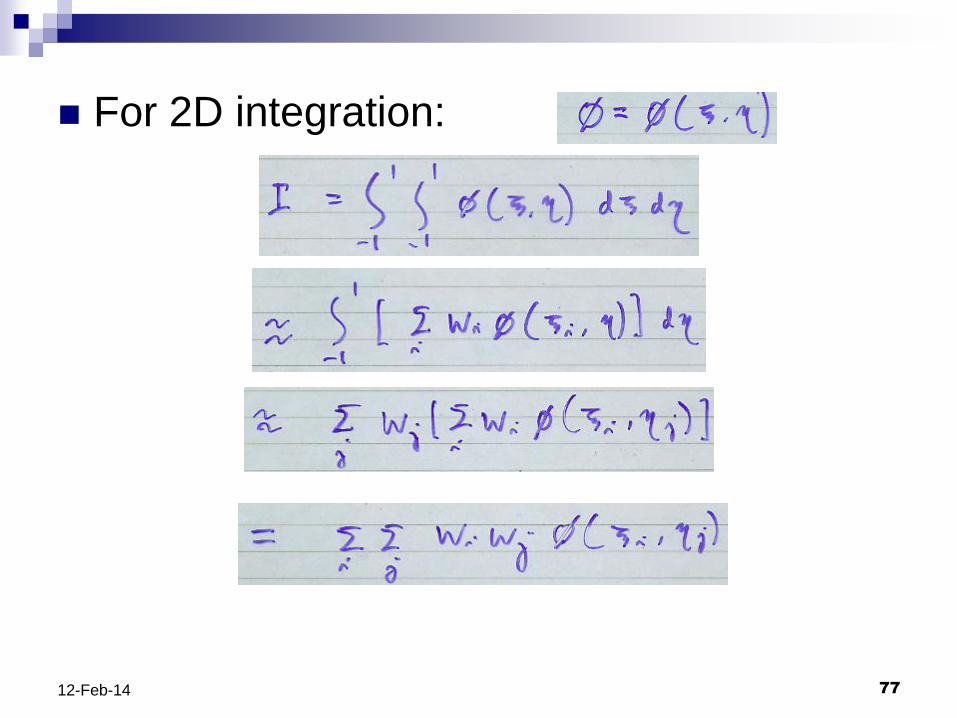
For 2D integration:

77 12-Feb-14

Gauss point locations in a quadrilateral

element using:

Four points (order 2 rule)

78 12-Feb-14

Nine points (order 3 rule)

79 12-Feb-14

Computation of stiffness matrix

80 12-Feb-14

If we use four sampling points:

81 12-Feb-14

ki: stiffness

matrix at

sampling point i

Computation of equivalent body

force

82 12-Feb-14

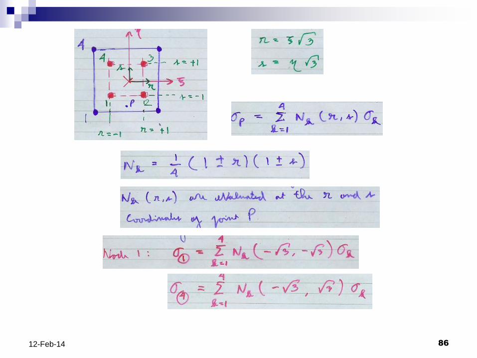
Stress evaluation

Once we have obtanied the nodal

displacement d from the direct stiffness

method, we can evaluate the stess at a

point of interest within the element using

We may evaluate the stess direcly at the

nodes.

83 12-Feb-14

Example

84 12-Feb-14

However, according to many FEM texts,

more accurate results can be achieved if

we evaluate the stresses first at the Gauss

points and then the stresses at the nodes

are extrapolated from those at the Gauss

points.

85 12-Feb-14

86 12-Feb-14

Degenerated Q4

If nodes 3 and 4 are coinsides, the

quadrilateral becomes a triangle

Another possibility

87 12-Feb-14

88 2014/2/12

Lecture Outline






6. References

1. Pure tension problem

For a thin plate in tension as shown in the figure,

determine the nodal displacements, support reactions,

and the stresses within the element

89 12-Feb-14

4 k

N/m

m

Dimension:

400 mm x 400 mm

h= 10 mm

E= 210 kN/mm2

ν= 0.3

The displacement

The support reactions

𝑅1 = 𝑅2 =400×4

2= 800 kN

The stress within the whole body

90 12-Feb-14

4 k

N/m

m R1

R2

These analytical results are useful for testing the

performence of the Q4 element

Suppose the the plate is discretized into two Q4

elements as follows

Compare the results from the finite element to the exact

solutions

91 12-Feb-14

4 k

N/m

m R1

R2

1 2 3

4

1

2

100 300

5 6

See the Matlab files Pure_tension_dat.m then

„Go‟

To see the resulting displacement, see the

content of variable Xdisp, DOF number 5 and 11

To see the resulting stresses at the nodes, see

the content of variables Stress

It can be seen that the resulting displacement,

support reactions and stresses are all exact!

Please check using your commercial software,

Strand.

92 12-Feb-14

2. Pure shear problem

For the same thin plate but in pure shear stress state as

shown in the figure, test the CST performance

93 12-Feb-14

The shear stress and shear modulus:

η = 𝑝

ℎ = 4000

10 = 400 N/mm2 = 0.4 kN/mm2

G = E

2:2𝑣 = 210000

2 : 2 x 0.3 = 80769 N/mm2 = 80.769 kN/mm2

The shear strain within the whole body

γ = τ

G =

400

80769.23077 = 0.004952381

The dispalcement of the top surface

D = 400 x 0.004952381 = 1.981 mm

94 12-Feb-14

See the Matlab files Pure_shear_dat.m then „Go‟

See the content of variable Xdisp, DOF number

7, 9, and 11

It can be seen that the resulting displacement,

support reactions and stresses are all exact!

How about the results from your software?

95 12-Feb-14

4 k

N/m

m

4 k

N/m

m

4 kN/mm

4 kN/mm

1

2

800

200 800 600

800

600 800 200

800

800

3. Pure bending problem

Consider a two dimensional body under pure bending

condition as shown in the figure.

Test the performance of the Q4 in this problem.

96 12-Feb-14

97 12-Feb-14

The deflection of the neutral axis according to the beam

bending theory:

Δ = 𝑀𝐿2

2𝐸𝐼 =

6666.7 × 1002

2 ×210 × 1

12× 20 × 403

= 1.4881 mm

Finite element model

See Pure_bending_dat

98 12-Feb-14

0 20 40 60 80 100

-10

0

10

20

30

40

50

1 2

3 4

1 2 3

4 5 6

7 8 9

Q4 Test: Pure Bending

X axis

Y a

xis

500/3

500/3

99 12-Feb-14

The deflection of the neutral axis from FEA using

different degrees of mesh refinement:

MESH Q4 Percentage

2x2 0.9154 61.5%

4x4

8x8

16x16

Exact 1.4881 100.0%

It needs a fine mesh to obtain Q4 accurate solution.

We can conclude that the performance of the Q4 is not

so satisfactory in bending problem.

4. Plane Elasticity Beam

The analytical solution for the (plane stress) cantilever beam

problem is given by Timoshenko and Goodier as follows:

5. Cook‟s Membrane Problem

101 12-Feb-14

48

44

16 C

F=

1.0

E=1.0, ν=1/3, and h=1.0

The reference solution: vC= 23.91

See

Cook_m4auto_d

at and

Cook_m8_dat

102 12-Feb-14

# elements

on each side

Q4 Percentage

4 18.30 76.5

8 22.08 92.3

16

Ref. soluion 23.91 100%

48

44

16 C

F=

1.0

6. An infinite plane-stress plate

with a hole

103 12-Feb-14

The plate subjected to uniform tension Tx at infinity

104 2014/2/12

Lecture Outline



3. Isoparametric elements Bilinear isoparametric quadrilateral

element


5. References

105 2014/2/12

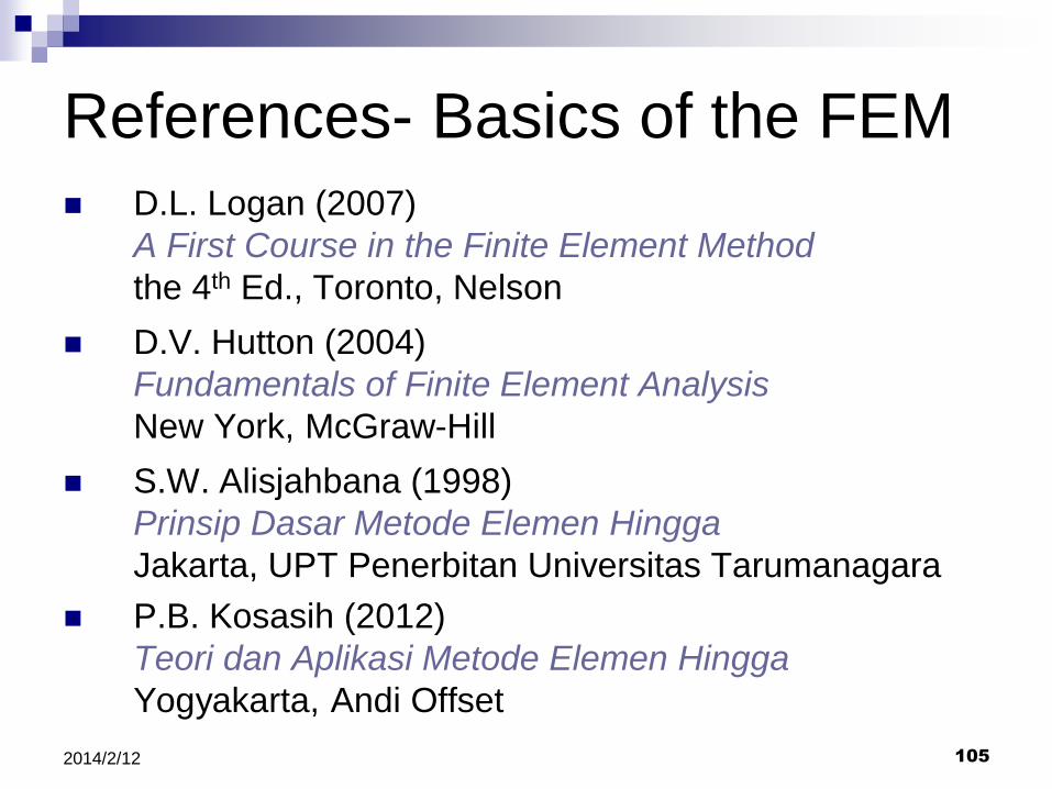
References- Basics of the FEM

D.L. Logan (2007)

A First Course in the Finite Element Method

the 4th Ed., Toronto, Nelson

D.V. Hutton (2004)

Fundamentals of Finite Element Analysis

New York, McGraw-Hill

S.W. Alisjahbana (1998)

Prinsip Dasar Metode Elemen Hingga

Jakarta, UPT Penerbitan Universitas Tarumanagara

P.B. Kosasih (2012)

Teori dan Aplikasi Metode Elemen Hingga

Yogyakarta, Andi Offset

106 2014/2/12

References- More Advance

R. D. Cook, D.S. Malkus, M.E. Plesha and R.J. Witt (2002)

Concepts and Applications of Finite Element Analysis

4th Ed., John Wiley and Sons

W. Weaver, Jr. and P.R. Johnston (1984)

Finite Elements for Structural Analysis

New Jersey, Prentice-Hall

K.J. Bathe (1996)

Finite Element Procedures


107 2014/2/12

References- Software Oriented

W. Dewobroto (2013)

Komputer Rekayasa Struktur dengan SAP2000


Computers and Structures, Inc. (2006)

SAP2000 Documentation, Berkeley, CSI

108 2014/2/12

References- Internet Resources

C. Felippa (2008)

Introduction to Finite Element Methods

http://www.colorado.edu/engineering/cas/courses.d/IFEM.d/

R. Krisnakumar (2010)

Introduction to Finite Element Methods

http://www.youtube.com

(Video of lecture series on FEMs)

K. J. Bathe (2009)

Finite Element Procedures for Solids and Structures

http://ocw.mit.edu/resources/res-2-002-finite-element-procedures-for-solids-and-structures-spring-2010/index.htm#



http://www.youtube.com/

http://ocw.mit.edu/resources/res-2-002-finite-element-procedures-for-solids-and-structures-spring-2010/index.htm























isoparametric finite elements - petra christian...

Documents