larger than one probabilities in mathematical and ...bapress.ca/ref/ref-2012-4/larger than one...

Review of Economics & Finance

Submitted on 02/May/2012

Article ID: 1923-7529-2012-04-01-13 Mark Burgin, and Gunter Meissner

~ 1 ~

Larger than One Probabilities in

Mathematical and Practical Finance

Mark Burgin

Department of Mathematics, University of California, Los Angeles

405 Hilgard Ave., Los Angeles, CA 90095, USA

E-mail: [email protected]

Gunter Meissner

MFE Program, Shidler College of Business, University of Hawaii

2404 Maile Way, Honolulu, HI 96822, USA

E-mail: [email protected]

Abstract: Traditionally probability is considered as a function that takes values in the interval [0,

1]. However, researchers found that negative, as well as larger than 1 probabilities could be a useful

tool in making financial modeling more exact and flexible. Here we show how larger than 1

probabilities could be handy for financial modeling. First, we define and mathematically rigorously

derive the properties of larger than 1 probabilities based on their frequency interpretation. We call

these probabilities inflated probabilities because conventional probabilities are never larger than 1.

It is transparently demonstrated that inflated probabilities emerge in various real life situations. We

then explain how inflated probabilities can be applied to modeling financial options such as Caps

and Floors. In trading practice, these options are typically valued in a Black-Scholes-Merton

framework, which assumes a lognormal distribution for the price of underlying assets. Since

negative values are not defined in the lognormal framework, negative interest rates cannot be

modeled. However interest rates have been negative several times in financial practice in the past.

We show that applying inflated probabilities to the Black-Scholes-Merton model implies negative

interest rates. Hence with this extension, Caps and Floors with negative interest rate can be

conveniently modeled closed form.

JEL Classifications: C10, G15, E22, E43, F34

Keywords: Interest rate; Caps; Floors; Negative interest rate; Inflated probabilities; Negative

probabilities; Black-Scholes-Merton model

ISSNs: 1923-7529; 1923-8401 © 2012 Academic Research Centre of Canada

~ 2 ~

1. Introduction

Traditionally probability is considered as a function that takes values in the interval [0, 1]

(Kolmogorov, 1933/1950). However, researchers found that probabilities values of which did not

belong to this interval could be useful in various situations. For instance, negative probabilities have

been applied to a number of theoretical and practical problems. At first, negative probabilities

appeared in physics, where they have become rather popular (see, for example, (Wigner 1932;

Dirac, 1942; 1943; Bartlett, 1945; Feynman 1950; 1987; Mückenheim, 1986; Krennikov, 1992;

2009)). Then negative probabilities came to finance (Haug, 2004; Székely, 2005; Burgin and

Meissner, 2011; 2012).

At the same time, larger than 1 probabilities, also called above unity probabilities or bigger

than one probabilities, i.e., probabilities values of which can be larger than 1, have received less

attention. One of the few to address them was Nobel Prize laureate Paul Dirac who wrote (1943):

“The various parts of the wave function which referred to the existence of positive

and negative-energy photons in the old interpretation now refer to the emissions and

absorptions of photons. The probabilities, equal to 2 and -2, are not physically

understandable, but one can use them mathematically in accordance with the rules for

working with a Gibbs ensemble.”

However, even before Dirac used and contemplated larger than 1 probabilities, they were

intrinsically brought into play by other physicists. In his fundamental review on extended

probabilities, Mückenheim (1986) explains how such probabilities emerge by extending the

quantum theoretical description of radiation given by Weisskopf and Wigner (1930). They

calculated the natural linewidth of radioactive decay of an excited atom in which the normalized

decay probability density (E, t) can take on negative values, as well as values exceeding unity. As

a result, the corresponding normalized probability, which is an observable quantity, may violate

both the lower and the upper limit in Kolmogorov‟s axioms (Mückenheim, 1986). It is important

that these results were verified by experiments, demonstrating that utilization of larger than 1

probabilities well reflected physical reality (Holland, et al, 1960; Lynch, et al, 1960; Wu, et al,

1960).

Another Nobel Prize laureate Richard Feynman (1987) also argued that larger than 1

probabilities could be useful for probability calculations in different problems of quantum physics.

Later larger than 1 probabilities have been considered in physics, biology and finance in the

works of Mack (2002), Sjöstrand (2006), Kovner and Lublinsky (2007), Venter (2007), and

Nyambuya (2011). Some of the researchers did not want to accept meaningfulness of larger than 1

probabilities and tried to eliminate them by some artificial transformations. For instance, Mack

(2002) tries to get rid of larger than 1 probabilities by reducing the probability mass at zero. Other

researchers recognized larger than 1 probabilities as an inherent property of the studied phenomena.

For instance, Haug (2004) argued that negative, as well as larger than 1 probabilities could be a

useful tool in enhancing financial modeling. Even more, Kronz (2009) explains necessity of greater

than one probabilities demonstrating that one can account for constructive quantum interference, if

probability values greater than one are allowed.

Gell-Mann and Hartle (2012) extended probability ensemble interpretation by including real

numbers that may be negative or greater than 1 as the probability values and providing an

unconventional interpretation of such probabilities. According to them, such extended probabilities

obey the usual rules of probability theory except that they can be negative or greater than one for an

alternative for which it cannot be determined whether it occurs or not (as on the alternative histories

in the two-slit experiment).


~ 3 ~

We also argue that larger than 1 (inflated) probabilities have sensible meaning, demonstrating

that they are well defined concepts in mathematics and useful in finance. For instance, we show that

larger than 1 probabilities can be applied to solving problems in financial modeling.

Looking into the history of mathematics and physics, we see that the evolution of negative, as

well as larger than 1 probabilities is similar to the development of many new concepts in

mathematics, which were initially met with skepticism. For instance, when negative numbers were

introduced, critics dismissed their sensibility. Some of the European mathematicians, such as

d‟Alembert or Frend, rejected the sensibility of negative numbers until the 18th century and referred

to them as „absurd‟ or „meaningless‟ (Kline, 1980; Mattessich, 1998). Even in the 19th century, it

was a common practice to ignore any negative results derived from equations, on the assumption

that they were meaningless (Martinez, 2005). For instance, Lazare Carnot (1753-1823) affirmed

that the idea of something being less than nothing is absurd (Mattessich, 1998). Such outstanding

mathematicians as William Hamilton (1805-1865) and August De Morgan (1806-1871) had similar

opinions. In the same way, irrational numbers and later imaginary numbers were firstly rejected.

Today these concepts are accepted and applied in numerous scientific and practical fields, such as

physics, chemistry, biology and finance. This situation shows that negative, as well as larger than 1

probabilities are finding more and more practical applications. Here we consider their application to

financial modeling, in particular, to option pricing.

The remaining paper is organized as follows. In section 2, we resolve the mathematical issue of

inflated (larger than 1) probabilities, demonstrating experimental situations when inflated

probabilities emerge and building mathematically grounded interpretations for inflated probabilities.

In section 3, we give examples of negative nominal interest rates in financial practice and

explain problems of current financial modeling of negative interest rates. In Section 4, we build a

mathematical model for Caps and Floors integrating inflated probabilities into the pricing model to

allow for negative interest rates. In Section 5, we explain how inflated probabilities emerge in

Duffie-Singleton model (Duffie and Singleton, 1999). Conclusions are given in Section 6.

2. Mathematical Foundations for Inflated Probability

In contrast to the wide-spread opinion, inflated, or larger than 1, probability has a natural

interpretation. To show this, let us consider the following situations.

Example 1. In an experiment, three coins are tossed. The conventional question is: What is the

probability of getting, at least, one head in one toss? To calculate this probability, we assume that

all coins are without defects and all tosses are fair and independent. Thus, the probability of having

heads (h) for one toss of one coin is p1(h) = 0.5. The same is true for tails (t). Thus, the probability

of having no heads or what is the same, of having three tails, in this experiment is p(0h) = p(3t) =

0.5 0.5 0.5 = 0.125.

At the same time, we may ask the question: What is the probability of getting heads in one toss

with 3 coins? To answer this question, let us suppose that probability reflects not only the average

of getting of heads (which is 0.5) but also the average number of obtained heads in one toss (it may

be 1.5, for example). In this case, the probability of having heads in tossing three coins once is p3(h)

= 0.5 + 0.5 + 0.5 = 1.5.

The difference between these two situations is that in the first case, getting one head and

getting two heads are different events (outcomes of the experiment). In contrast to this, in the

second case, getting one head and getting two heads are different parts of the same event, or better

to say, the same multi-event (parts of the same outcome of the experiment). It means that an


~ 4 ~

outcome may have a weight, e.g., when two heads occur, the weight is 2, while when three heads

occur, the weight is 3.

Note that with the growth of the number of the tossed coins, the probability of having heads

also grows being larger than 1 when there are more than two coins.

Example 2. In an experiment, 10 dice are rolled. Let us ask the question: What is the

probability of showing three spots in one experiment? To calculate this probability, we assume that

all dice are without defects and all rollings are fair and independent. In this case, the probability of

having three spots in one rolling is p1 = 1/6 for one die and p10 = 10/6.

Now we can describe a general schema for frequency interpretation of inflated or larger than 1

probability.

As usually, we start with elementary (random) events but instead of a set of these events, we

consider a multiset Ω of elementary (random) events. Informally, a multiset is a collection that is

like a set but can include identical or indistinguishable elements (Aigner, 1979; Knuth, 1997). Thus,

we take a multiset Ω = { n1w1 , n2w2 , n3w3 , … , nkwk }. In it, wi are elementary events, or more

exactly, types of elementary events and ni is the multiplicity, i.e., the number, of copies of the

elementary event wi in Ω for all i = 1, 2, 3, … , k. For instance, {3a, 7b} is the multiset {a, a, a, b,

b, b, b, b, b, b}, which contains three elements a and seven elements b. To be exact, {3a, 7b} is the

multinumber (cardinality) of the multiset {a, a, a, b, b, b, b, b, b, b} (Burgin, 2011), but many

researchers used multinumbers as representations of multisets and for simplicity, we follow this

tradition.

Subsets of the multiset Ω are called events. For instance, {a, 3b} and {5b} is the submultiset

but not a subset of the multiset {3a, 7b}. At the same time, {a, b} and {b} are subsets of the

multiset {3a, 7b}. In other words, a subset of a multiset A are sets such that their elements are also

elements of A.

We assume that the following axiom is true.

Decomposability Axiom. An event A occurs in a trial if and only if some elementary event

from A occurs in this trial.

However, when we have a multiset of elementary events, it is natural to assume, as in the

examples considered above, that it is possible that several elementary events from A and even

several elementary events of the same type from A occur in one trial. To formalize this situation, we

use the following axiom.

Boundary Axiom. The number of occurrences of an elementary event wi from A in one trial

cannot be larger than the multiplicity ni of this event in Ω.

Taking an event A = {wi1 , wi2 , wi3 , … , wir} and a sequence of N trials, we denote by N the

number of events from Ω that occur during this sequence of trials and by n the sum of multiplicities

of events from A that occur during this sequence of trials. Then we have the frequency

rN(A) = n/N

In contrast to conventional trials it is possible that rN(A) > 1 because the same event can occur

several times in one trial. For instance, if A occurs 3 times in each of N trials, then rN(A) = 3.

Let us consider the set PA of all events A such that limits limN rN(A) exist. We call these

events quasirandom. Random events satisfy additional conditions considered by different authors.

Then we define the inflated frequency probability of the event A as

p(A) = limN rN(A)


~ 5 ~

In other words, when the number N of trials goes to infinity (N ) the number rN(A )

approaches the inflated frequency probability of the event A. The regularity of rN(A) converging to a

proper fraction characterizes the meaning of the probability of the event A.

Note that the conventional frequency probability is a particular case of the inflated frequency

probability when elementary events form a set, i.e., all their multiplicities are equal to 1.

Let us study properties of inflated frequency probabilities. It is easy to see that they do not

satisfy standard probability properties. For instance, in a general case, p(Ω) > 1.

However, some standard probability properties remain true. Properties of limits imply the

following result.

Proposition 1. The inflated frequency probability p of the union of two disjoint quasirandom

events A and B is equal to p(A B) = p(A) + p(B), i.e., A ∩ B = Ø implies p(A B) = p(A) + p(B).

Usually it is assumed that p(Ø) = 0. However, this property also depends on the initial axioms.

Let us consider two such axioms.

Occurrence Axiom. In any trial, at least one elementary event occurs.

Weak Occurrence Axiom. In any trial, at least one event occurs.

Lemma 1. The Occurrence Axiom implies the Weak Occurrence Axiom.

Proposition 2. If the Occurrence Axiom is true, then the inflated frequency probability,

probability p of the empty event is equal to zero.

Lemma 2. The Decomposability Axiom and Weak Occurrence Axiom imply the Occurrence

Axiom.

Corollary 1. If the Decomposability Axiom is true, then the inflated frequency probability p of

the empty event is equal to zero.

Trying to find a criterion, i.e., the necessary and sufficient conditions, for the equality p(Ø) = 0,

we come to the following axiom.

Finite Occurrence Axiom. In any sequence of trials, there is only a finite number of trials

when at least one elementary event does not occur.

However, we also need a weaker condition.

Infinite Occurrence Axiom. In any sequence of trials, there are an infinitely many trials when

at least one elementary event occurs.

This axiom allows us to prove the following result.

Proposition 3. The inflated frequency probability p(Ø) is equal to zero if and only if the ratio

of all trial in which nothing happened to all trials tends to 0.

Corollary 2. The inflated frequency probability p(Ø) is equal to zero only if the Infinite

Occurrence Axiom is true.

Corollary 3. The inflated frequency probability p(Ø) is equal to zero if the Finite Occurrence

Axiom is true.

Finite Occurrence Condition. In any sequence of trials, there only a finite number of trials

when an elementary event from A occurs.

This condition allows us to prove the following result.

Proposition 4. The inflated frequency probability p(A) of a quasirandom (random) event A is

equal to zero if the Finite Occurrence Condition is true.


~ 6 ~

Corollary 4. The inflated frequency probability p(A) of a quasirandom (random) event A is not

equal to zero only if the Infinite Occurrence Axiom is true.

Many properties of inflated frequency probabilities are different from the standard probability

properties.

Proposition 5. The inflated frequency probability p(A) of a quasirandom (random) event A

cannot be larger than the sum of the multiplicities of the elements from A, i.e., if A = {wi1, wi2, wi3,

… , wir}, then

p(A) ni1 + ni2 + ni3 + … + nir

where ni1, ni2, ni3, … , nir are multiplicities of the elements wi1, wi2, wi3, … , wir in the multiset Ω.

The constructed interpretation is similar to the traditional frequency interpretation of

probability. However, in our situation, several elementary events from A can occur in one trial.

Let us consider the following axiom.

Outcome Axiom (OA). In each trial, exactly one elementary event happens.

Note that it can be several occurrences (copies) of one and the same elementary event in one

trial.

We can see that when the Outcome Axiom is taken instead of the Boundary Axiom, we exactly

obtain the traditional frequency interpretation of the classical probability.

This interpretation explains why larger than 1 (inflated) probabilities, at first, appeared in

quantum physics and then proliferated to other disciplines. Indeed, according to modern quantum

physics, all subatomic particles, such as electrons, protons or neutrons, are identical or

indistinguishable. As a result, collections of subatomic particles are multisets and not sets because

in sets according to the modern set theory all elements are distinguishable from one another

(Fraenkel and Bar-Hillel, 1958; Kuratowski and Mostowski, 1967).

It is possible to construct another formalization of inflated (larger than 1) probabilities when

instead of the Boundary Axiom, we use the following axiom.

Single Type Axiom. In each trial, elementary events of only one type happen and their number

cannot be larger than the multiplicity of this element in the multiset Ω.

Note that the Single Type Axiom implies the Boundary Axiom.

Proposition 6. If the Single Type Axiom is valid, then the inflated frequency probability p(A)

of a quasirandom (random) event A cannot be larger than the maximum of the multiplicities of the

elements from A, i.e., if A = {wi1 , wi2 , wi3 , … , wir}, then

p(A) max { ni1 , ni2 , ni3 , … , nir }

where ni1, ni2, ni3, … , nir are multiplicities of the elements wi1, wi2, wi3, … , wir in the multiset Ω.

As the conventional frequency probability is a particular case of the inflated frequency

probability when multiplicities of all elementary events are equal to 1, we have the classical

property of probability.

Corollary 5. If the Single Type Axiom is true, then the frequency probability p(A) of the empty

event is equal to zero.

Conventional probability also has a subjective interpretation, which is identified as a belief or

measure of confidence in an outcome of a certain event. In some cases, an adequate treatment of

subjective interpretations brings researchers to inflated probabilities. To show this, let us consider

the following situation.


~ 7 ~

In a criminal investigation, the detective gets some evidence that strongly shows that the main

suspect is not guilty. To express his confidence, the detective says: “Oh, I‟m 70% sure that this

woman is not guilty.” According to the subjective interpretation, 70% mean that the probability of

the woman‟s innocence is 0.7.

After some time, the detective gets even more persuading evidence and when asked by his

chief, the detective says: “Now I‟m two times more confident that this woman is not guilty.”

However, two times 70% gives us 140% and according to the conventional probability theory, this

is impossible because 140% mean that the probability of the woman‟s innocence is 1.4, while larger

than 1 probabilities are not permitted. However, if we allow larger than 1 probabilities, the

statement of the detective becomes clear.

This situation and many other similar situations, for example, in financial decision making,

show that inflated probabilities have a meaningful subjective interpretation and this interpretation

allows people to explain not only phenomena in physics or finance but many situations in their

everyday life.

3. Negative Interest Rates and the Problem of Their Modeling

3.1 Situations When Nominal Interest Rates Became Negative

Negative nominal interest rate are a seldom phenomenon in financial practice. However, they

have occurred several times as in the 1970s in Switzerland. Investors had invested at negative

interest rates in the safe haven Switzerland since they believed the Swiss Franc would increase. In

addition, some investors avoided paying taxes in their home country. Negative interest rates also

occurred in Japan in the 1990s, in 2003 in the USA and during the global financial crisis 2008/2009.

For instance, in Japan in the 1990s, banks lent Japanese Yen and were willing to receive a

lower Yen amount back several days later. This means de facto a negative nominal interest rate. The

reason for this unusual practice was that banks were eager to reduce their exposure to Japanese Yen,

since confidence in the Japanese economy was low and the Yen was assumed to devalue.

Similarly, in the US, from August to November 2003, „repos‟, i.e. repurchase agreements, were

traded at negative interest rates. A repo is just a collateralized loan, i.e. the borrower of money gives

collateral, for example a Treasury bond, to the lender for the time of the loan. When the loan is paid

back, the lender returns the collateral. However, in 2003 in the US, settlement problems when

returning the collateral occurred. Hence the borrower was only willing to take the risk of not having

the collateral returned if he could pay back a lower amount than originally borrowed. This

constituted a negative nominal interest rate.

A further example of the market expecting the possibility of negative nominal interest rates

occurred in the worldwide 2008/2009 financial crisis, when strikes on options on Eurodollars

Futures contracts were quoted above 100. A Eurodollar is a dollar invested at commercial banks

outside the US. A Eurodollar futures price reflects the anticipated future interest rate. The rate is

calculated by subtracting the Futures price from 100. For example, if the 3 month March Eurodollar

future price is 98.5, the expected interest rate from March to June is 100 – 98.5 = 1.5, which is

quoted in per cent, so 1.5%. In March 2009, option strikes on Eurodollar future contracts were

quoted above 100 on the CME, Chicago Mercantile Exchange. This means that market participants

could buy the right to pay a negative nominal interest on US dollars in the future if desired. The

reason for this unusual behavior is that investors wanted to invest in the safe haven currency US

dollar even if they had to pay for it.


~ 8 ~

3.2 Modeling Interest Rates

In finance, interest rates are typically modeled with a geometric Brownian motion,

dtε σ dt μr

drrr (1)

dr is the change in the interest rate r, r is the drift rate, which is the expected growth rate of r,

assumed non-stochastic and constant, r is the expected volatility of the rate r, assumed non-

stochastic and constant, is a random drawing from a standardized normal distribution. All

drawings at times t are independent.

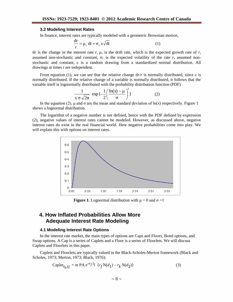
From equation (1), we can see that the relative change dr/r is normally distributed, since is

normally distributed. If the relative change of a variable is normally distributed, it follows that the

variable itself is lognormally distributed with the probability distribution function (PDF)

}σ

μln(x)

2

1exp{-

2π σx

12

(2)

In the equation (2), μ and σ are the mean and standard deviation of ln(x) respectively. Figure 1

shows a lognormal distribution.

The logarithm of a negative number is not defined, hence with the PDF defined by expression

(2), negative values of interest rates cannot be modeled. However, as discussed above, negative

interest rates do exist in the real financial world. Here negative probabilities come into play. We

will explain this with options on interest rates.

Figure 1. Lognormal distribution with μ = 0 and σ =1

4. How Inflated Probabilities Allow More Adequate Interest Rate Modeling

4.1 Modeling Interest Rate Options

In the interest rate market, the main types of options are Caps and Floors, Bond options, and

Swap options. A Cap is a series of Caplets and a Floor is a series of Floorlets. We will discuss

Caplets and Floorlets in this paper.

Caplets and Floorlets are typically valued in the Black-Scholes-Merton framework (Black and

Scholes, 1973; Merton, 1973; Black, 1976):

Capletts,tl = m PA e-rl tl {rf N(d1) – rk N(d2)} (3)


~ 9 ~

Floorletts,tl = m PA e-rl tl {rk N(-d2) – rf N(-d1)} (4)

where d1 =

x

x

2

k

f

tσ

tσ2

1)

r

rln(

, and d2 = d1 - xtσ

.

Capletts,tl is the option on an interest rate from time ts to time tl, where tl > ts , i.e., it means the

right but not the obligation to pay the rate rK at time tl .

Floorletts,tl is the option on an interest rate from time ts to time tl, where tl > ts, i.e., it means the

right but not the obligation to receive the rate rK at time tl . Here m is time between ts and tl,

expressed in years; tx is the option maturity time; tx ≤ ts < tl; PA is the principal amount; rK is the

strike rate, i.e., the interest rate that the Caplet buyer may pay and the Floorlet buyer may receive

from time ts to time tl; and ltst

,fr is the forward interest rate from ts to tl, derived as

(5)

where df is a discount factor, i.e. dfty = 1/(1 + ry).

4.2 Applying Inflated Probabilities to Caplets and Floorlets

As it is demonstrated above, the market applied lognormal distribution, which is underlying the

valuation of interest rate derivatives, cannot model negative interest rates. One seeming solution

would be to add a location parameter to the lognormal distribution. Hence equation (1) 2

σ

μln(x)

2

1-

e 2π σx

1

becomes

2

σ

μα)-ln(x

2

1-

e 2π σ α)-(x

1

, where α is the location parameter. For

α > 0, the lognormal distribution is shifted to the right. As a result, the probabilities to the right of

the mean would increase, which gives the desired result (see below for details). However,

probabilities to the left of the mean would decrease, which is undesired. Hence this solution is

inapplicable.

A consistent way to model options on negative interest rates is to apply inflated probabilities to

equations (3) and (4). We add a parameter β to equations (3) and (4) and for simplicity, we set m =

1 and PA =1. Hence we derive

Capletts,tl = e-rl tl {rf [N (d1)-β] – rk [N(d2)-β]} β (6)

Floorletts,tl = e-rl tl {rk [N(-d2)-β] – rf [N(-d1)-β]} (7)

where d1 =

x

x

2

k

f

tσ

tσ2

1)

r

rln(

and d2 = d1 - ltσ.

This brings us to inflated probabilities which can imply negative interest rates. Let‟s show this.

From basic option theory we know that the value of a Floorlet is divided into intrinsic value IV and

time value TV:

sllt

st

,ftt

1 1

df

dfr

ltst


~ 10 ~

Floorlet ts,tl = IVFloorlet + TVFloorlet ≥ 0 (8)

The intrinsic value is defined IVFloorlet = max (rk – rf, 0), where rf is derived by equation (5). For

simplicity we assume that the yield curve is flat. It follows that r = rf and we derive

IVFloorlet = max (rk – r, 0) (9)

Let‟s investigate the case of the Floorlet being in-the-money and the Caplet being out-of-the-

money i.e. rk > r. Hence equation (9) changes to

IVFloorlet = rk – r (10)

Since a Floorlet does not pay a return, the time value of a Floorlet is bigger than 0,

TVFloorlet ≥ 0 (11)

With a negative β, inflated probabilities can emerge for certain input parameter constellations

of equations (6) and (7). In particular, the probabilities N(d1)- β, N(d2)- β, N(-d2)- β and N(-d1)- β

may become larger than 1. In this case, from equation (7), the resulting Floorlet price can become,

especially for low implied volatility, smaller than the intrinsic value, i.e. Floorlet ts,tl < IVFloorlet .

From equations (8), (10), and (11), this implies that r < 0 for small values of rK. Hence we have an

extension of the lognormal distribution with inflated probabilities associated with negative values

for r. Graphically this can be expressed by an upward shift of the lognormal distribution (see Figure

1), which creates a PDF function with a probability area larger than one.

The lower the value of β, the more likely it is that inflated probabilities with associated

negative interest rates will emerge. This lowers Caplet prices and increases the Floorlet price, which

is a desired result, since it adjusts the Caplet and Floorlet prices for the possibility of negative

interest rates. The magnitude of the parameter β, that a trader applies, reflects a trader‟s opinion on

the possibility of negative rates. The lower, including negative interest rates, a trader expects, the

lower is the beta she will input in equations (6) and (7).

Let us combine these results with the results derived for negative probabilities in the paper on

negative interest rates, Burgin and Meissner (2011). We observe that depending on the parameter

constellations of the Black-Scholes-Merton model in some cases negative probabilities and in some

cases inflated probabilities imply negative interest rates. In particular, in the case of rk < r, negative

probabilities imply negative interest rates. In this case the lognormal distribution is extended to the

left as seen in Figure 2:

Figure 2: An extension of the lognormal distribution with μ = 0 and σ =1


~ 11 ~

In the case when r < rk , inflated probabilities imply negative interest rates, as derived above. In

this case the lognormal distribution of Figure 1 is shifted upwards to create a probability space of

bigger than 1.

5. Duffie-Singleton Model and Inflated Probabilities

We find a further application of inflated probabilities in the seminal Duffie-Singleton model

(Duffie and Singleton, 1999). They prove that a defaultable claim can be priced “if it were default

free by replacing the usual short-term interest rate process r with the default-adjusted short-term

process Rt = r + htL”, where L is the loss in default, i.e. L = 1 - RR where RR is the recovery rate

and ht is the hazard rate at t, i.e. the default probability from t to t + dt assuming no default until t.

Discounting with Rt results in the value of the defaultable claim V at time 0, V0.

T

0

tQ00 dtRexpEV (12)

where Q0E is the risk-neutral expectation under the equivalent martingale measure Q at date 0.

For ease of explanation, let us set r = 0 and RR = 0 so, that L = 1. As a result Rt = ht and

equation (12) changes to

T

0

tQ00 dthexpEV (13)

Utilization of the conventional probability theory creates a discrepancy between the equation

(13) and extreme values of the hazard rate ht. By the conventional probability definition, the value

ht is limited to 1. However, in the extreme case of ht = 1, i.e., when there is a certain default, the

defaultable claim V0 should be zero. However equation (13) implies V0 > 0 when ht ≤ 1. Rather than

discarding the whole model, we suggest a solution, namely, introduction of a possibility that the

hazard rate ht can be larger than 1. Then taking the limit limt ht → ∞, we see that equation (13)

gives the correct value of the defaultable claim V0 of 0.

6. Concluding Summary

We defined generalized probabilities, which include inflated probabilities, build their

interpretations and derived their general properties. Then we applied generalized probabilities to

financial modeling demonstrating that negative nominal interest rates have occurred several times in

the past in financial practice, for example, in the 2008/2009 global financial crisis. This is

inconsistent with the conventional theoretical models of interest rates, which typically apply a

lognormal distribution. In particular, when Caps and Floors are valued in a lognormal Black-

Scholes-Merton framework, then the probability of negative interest rates is zero. Here larger than 1

probabilities come into play. We demonstrated that for in-the-money Floors and out-of-the-money

Caps, i.e., with the parameter constellation r < rk , integrating inflated probabilities into the Black-

Scholes-Merton framework allows one to consistently model negative nominal interest rates, which

occur in financial practice.


~ 12 ~

References

[1] Aigner, M.(1979), Combinatorial Theory, Springer Verlag, New York/Berlin.

[2] Bartlett, S.( 1945), “Negative Probability”, Math Proc Camb Phil Soc, 41: 71–73.

[3] Black F. and M. Scholes (1973), “The Pricing of Options and Corporate Liabilities”, The

Journal of Political Economy, 81(3): 637-654.

[4] Black, F. (1976), “The Pricing of Commodity Contracts”, Journal of Financial Economics, 3(1-

2): 167-179.

[5] Burgin, M. (2011), Theory of Named Sets, Nova Science Publishers, New York.

[6] Burgin, M. and Meissner, G. (2011), “Negative Probabilities in Modeling Random Financial

Processes”, Integration, 2(3): 305 – 322.

[7] Burgin, M. and G. Meissner (2012), “Negative Probabilities in Financial Modeling”, Wilmott

Journal, 2012(58): 60 – 65.

[8] Dirac, P.A.M. (1942), “The Physical Interpretation of Quantum Mechanics”, Proc. Roy. Soc.

London, 180(980): 1–39.

[9] Dirac, P.A.M. (1943), Quantum Electrodynamics, Communications of the Dublin Institute for

Advanced Studies.

[10] Duffie, D. and Singleton, K. ( 1999), “Modeling Term Structures of Defaultable Bonds”,

Review of Financial Studies, 12(4): 687-720.

[11] Feynman, R. P. (1950), “The Concept of Probability Theory in Quantum Mechanics”, In: The

Second Berkeley Symposium on Mathematical Statistics and Probability Theory, University of

California Press, Berkeley, California.

[12] Feynman, R. (1987), “Negative Probability”, In: Quantum Implications: Essays in Honour of

David Bohm, Routledge & Kegan Paul Ltd, London & New York, pp. 235–248.

[13] Fraenkel, A.A. and Bar-Hillel, Y. (1958), Foundations of Set Theory, North Holland P.C.,

Amsterdam.

[14] Gell-Mann, M. and Hartle, J. B. (2012), “Decoherent Histories Quantum Mechanics with One

'Real' Fine-Grained History”, Physical Review A, 85(6): 21-31.

[15] Haug, E.G.(2004), “Why so Negative to Negative Probabilities?”, Wilmott Magazine, Sep/Oct

2004: 34- 38.

[16] Holland, R. E. , F. J. Lynch, G. J. Perlow and S. S. Hanna (1960), “Time Spectra of Filtered

Resonance Radiation of Fe57

,” Phys. Rev Let., 4(4): 181-182.

[17] Khrennikov, A.(1992), “p-adic probability and statistics”, Dokl. Akad. Nauk, v.322, p.1075-

1079.

[18] Khrennikov, A. (2009), Interpretations of Probability, Walter de Gruyter, Berlin/New York.

[19] Kline, M. (1980), Mathematics: The Loss of Certainty, Oxford University Press, New York.

[20] Knuth, D. (1997), The Art of Computer Programming, v.2: Semi-numerical Algorithms,

Addison-Wesley, Reading, Mass.

[21] Kolmogorov, A. N. (1933), Grundbegriffe der Wahrscheinlichkeitrechnung, Ergebnisse Der

Mathematik (English translation: Foundations of the Theory of Probability, Chelsea P.C.,

1950).

[22] Kovner, A. and M. Lublinsky (2007), “Odderon and seven Pomerons: QCD Reggeon field

theory from JUMWLK evolution”, Journal of High Energy Physics, 58(1):1-61.


~ 13 ~

[23] Kronz, F. (2009), “Actual and Virtual Events in the Quantum Domain”, Ontology Studies,

9(9): 209-220.

[24] Kuratowski, K. and Mostowski, A. (1967), Set Theory, North Holland P.C., Amsterdam.

[25] Lynch, F. J., R. E. Holland, and M. Hamermesh (1960), “Time dependence of resonantly

filtered gamma rays from Fe57

,” Phys. Rev. 120(2): 513- 520.

[26] Mack, T.(2002), Schadenversicherungsmathematik, 2nd

ed. Verlag Versicherungswirtschaft.

[27] Martinez, A.A. (2005), Negative Math: How Mathematical Rules Can Be Positively Bent,

Princeton University Press, Boston.

[28] Mattessich, R. (1998), “From accounting to negative numbers: A signal contribution of

medieval India to mathematics”, Accounting Historians Journal, 25(2): 129 – 145.

[29] Meissner, G.(1998), Trading Financial Derivatives – Futures, Swaps, and Options in Theory

and Application, Pearson.

[30] Meissner. G.(1999), Arbitrage Opportunities in Fixed Income Markets, Derivatives Quarterly,

5(1): 1-8.

[31] Merton R. (1973), “Theory of Rational Option Pricing”, Bell Journal of Economics and

Management Science, 4(1): 141-183.

[32] Mückenheim, W. (1986), “A review of extended probabilities”, Physics Reports, 133(6): 337-

401.

[33] Nyambuya, G.(2011), Deciphering and Fathoming Negative Probabilities in Quantum

Mechanics?(viXra.org > Quantum Physics > viXra:1102.0031).

[34] Sjöstrand, T. (2007), “Monte Carlo Generators”, In: 2006 European School of High-Energy

Physics, Ed. R. Fleischer, CERN-2007-005, p. 51-73.

[35] Székely, G.J.(2005), “Half of a Coin: Negative Probabilities”, Wilmott Magazine, July: 66–68.

[36] Venter G. (2007), “Generalized Linear Models Beyond the Exponential Family with Loss

Reserve Applications”, Astin Bulletin, 37(2): 345-364.

[37] Weisskopf V., and E. Wigner (1930), “Berechnung der nat urlichen Linienbreite auf Grund der

Diracschen Lichttheorie”, Z. Phys., 63(1-2): 54-73.

[38] Wigner, E. P. (1932), “On the quantum correction for thermodynamic equilibrium”, Phys. Rev.,

40(5): 749-759.

[39] Wu, C. S. , Y. K. Lee, N. Benczer-Koller, and P. Simms (1960), “Frequency Distribution of

Resonance Line Versus Delay Time”, Physical Review Letters, 5(9): 432-435.

larger than one probabilities in mathematical and ...bapress.ca/ref/ref-2012-4/larger than one...

Documents