knife-edge scanning microscope (kesm 1.5): optics …department of computer science texas a&m...

KESM 1.5 Optics and Cameras

- 1 -

Knife-Edge Scanning Microscope (KESM 1.5):

Optics and Cameras Bruce H. McCormick

Department of Computer Science

Texas A&M University

College Station, TX, USA 77843-3112

[email protected]

Technical Report: tamu-cs-tr-2006-10-1


- 2 -

Abstract Knife-Edge Scanning Microscopy (KESM) is being developed for its potential applications to biology and medicine, and specifically for the scanning and reconstruction of whole organs at a cellular level of detail. This is the challenge that KESM 1.5, the extensive modification to the prototype instrument, KESM 1.0, is designed to address. In the new instrument, KESM 1.5, now under design and construction, tissue is sectioned and imaged concurrently. The plastic-embedded tissue is mounted under water in a specimen tank above a three-axis Aerotech stage. Only the stage, and hence specimen block, move; the diamond knife used for sectioning and the microscope/camera used for imaging are rigidly mounted to a granite bridge over the stage. The stage provides 20nm encoding on the two horizontal directions, X & Y, and 25nm in the Z-axis vertical lift stage. The microscope images the top facet of the diamond knife, and a line-scan camera scans the sectioned tissue as it flows across the top facet of the knife. Sections are typically cut at 0.5µm thickness. The lift stage is incremented in height by the section thickness after each cutting stroke. Because of the encoding accuracy of the stage, registration between images from serial sections has been excellent in KESM 1.0, allowing reconstruction of the cellular structure of the embedded tissue, for example, mouse brain. This technical report describes the following facets of KESM 1.5 design:

• Objectives, tube lenses, and optical trains • Line-scan cameras • Line-scan camera couplers • Observation camera and its coupler, and • Microscope/knife mounting

Each section gives the rationale for making the specified design choices. The design presented here accommodates both bright-field and fluorescence microscopy. However, the present technical report does not describe the illumination system of the KESM 1.5 instrument, except in general terms, nor does it model the flow of illumination from light source to the line-scan camera sensor. A companion technical report, KESM 1.5. Illumination for Bright-field and Fluorescence Microscopy, now in preparation, will return to this part of a comprehensive image capture system for KESM 1.5.


- 3 -

Table of Contents 1. Introduction

1.1. Rationale for KESM 1.5 optics and cameras 1.2. Versatile design to meet changing uses and technology 1.3. Overview of the instrument 1.4. Topics discussed

2. Objectives, Tube Lenses, and Optical Trains 2.1 Rationale for hybrid optical design of microscope 2.2 Olympus and Zeiss microscope objectives 2.3 Magnification and field of view in specimen plane 2.4 Olympus and Zeiss tube lenses 2.5 Optical trains

3. Line-scan Cameras 3.1 Limits on useable number of pixels 3.2 Cameras categorized by number of pixels 3.3 Cameras categorized by color and sensitivity 3.4 Cameras categorized by data rate 3.5 Output and control 3.6 Initial KESM 1.5 cameras

4. Line-Scan Camera Couplers 4.1 Grouping line-scan cameras by coupler 4.2 Line-scan couplers

5. Observation Camera and its Coupler 5.1 Uses of the observation camera 5.2 Choice of the observation camera 5.3 Couplers for the observation camera

6. Knife/Microscope/Camera Mounting 6.1 Knife/microscope axes define a three-dimensional Euclidean coordinate system 6.2. Optical components and camera mounting

6.2.1. Objectives 6.2.2. Magnification changer (Olympus optics only) 6.2.3. Universal reflected light illuminator with lamphouse and lasers 6.2.4. Dual port with tube lenses (Olympus and Zeiss) 6.2.5. Observation camera and couplers 6.2.6. Line-scan camera couplers 6.2.7. Line-scan cameras and their mounting

6.3 Knife assembly components and adjustments 6.3.1. Diamond knife and knife module 6.3.2. Knife mounting and adjustments 6.3.3. Ribbon extractor and pump

6.4. Specimen tank 6.3.1 Specimen tank

6.3.2. Specimen ring 6.3.3. Extraction of microscope/knife from specimen tank 6.3.4. Constrained movement of tank

Appendix A. Dalsa Line-Scan Cameras


- 4 -

A.1. First-generation KESM cameras A.2. Piranha P2-series line-scan cameras A.3. Piranha P3-series line-scan cameras A.4. Piranha HS-series line-scan cameras A.5. New Piranha P2 color line-scan

Appendix B. Comparison of Microscopes for Bright-field and Fluorescence Imaging

List of Tables Table 1. Water-immersion objective parameters Table 2. Magnifications and fields of view in specimen plane Table 3. Tube lens parameters Table 4. KESM 1.5 optical trains Table 5. Useable number of pixels for KESM 1.5 optics Table 6. Useable number of pixels for various effective objective magnifications Table 7. Cameras characterized by choice of stain technology Table 8. Dalsa line-scan cameras categorized by color and sensitivity Table 9. Available cameras categorized by data rate: pixel rate/(line/frame) rate Table10. Initial KESM 1.5 cameras Table11. Available cameras listed by increasing sensor diameter Table12. Coupler specifications Table13. Line-scan camera couplers used in KESM 1.5 Table14. Observation camera parameters Table15. Couplers for the observation camera Table16. Dual port tube lenses Table A.1. CT-series cameras used in KESM 1.0 Table A.2. Piranha2 P2-series cameras Table A.3. Piranha3 P3-series cameras Table A.4. Piranha2 HS-series cameras Table A.5. New Piranha2 color cameras (anticipated December 2006, preliminary data) Table B.1. Comparative study of four microscope systems

List of Figures Fig. 1. Objective position and orientation with respect to the diamond knife Fig. 2. Concurrent sectioning and imaging of specimen block. (a) Mouse brain in

specimen ring; (b) Tissue ribbon rolling across top facet of diamond knife (graphic visualization)

Fig. 3. Layout of KESM 1.5 optical trains Fig. 4. Knife/microscope axes define 3D regular Cartesian coordinate system Fig. 5. Magnification changer Fig. 6. Universal reflected light illuminator (URLI) Fig. 7. Modified URLI with dual laser ports Fig. 8. Mounting of Olympus Super 20X objective to the magnification changer (MC)

and universal reflected light illuminator (URLI) Fig. 9. Mounting of Zeiss 63X objective to magnification changer (MC) and universal

reflected light illuminator (URLI) Fig. 10. Dual port (side view) Fig. 11. Observation camera and coupler (schematic) Fig. 12. Adjustment of knife orientation


- 5 -

1. Introduction 1.1 Rationale for KESM 1.5 optics and cameras Knife-Edge Scanning Microscopy (KESM) is being developed for its potential applications to biology and medicine, and specifically for the scanning and reconstruction of whole organs at a cellular level of detail. No small-animal organ (e.g., brain, cardiovascular system, kidneys, or liver, as large as several hundred cubic millimeters in volume), has yet been scanned at submicron resolution, reconstructed in three dimensions, and visualized. Though visualized piecemeal through microscope binoculars, the anatomy of specimens only one-tenth this volume remains largely descriptive. Quantitative anatomy of tissue on a cellular scale, including visualizing its microstructure and statistically analyzing its cells and their interconnections, remains yet to be done. This is the challenge that KESM 1.5, the extensive modification to the prototype instrument, KESM 1.0, is designed to address. The reconstruction of the mouse brain, which is the focus of our current research efforts, remains a significant challenge for light microscopy. Diffraction-limited optics must be pushed to its limits to resolve fine structure in the brain--its dendritic spines and extensive fiber tracts of axons. The meshwork of fibers must be resolved to reconstruct the mouse brain network. We need the finest light microscope objectives and line-scan cameras available for such high-resolution biomedical imaging. High resolution comes at a high cost: Every improvement by a factor of two in linear resolution of the specimen demands an eight-fold increase in scanning time, computation, and data storage. Therefore we also need a complementary facility to survey organs targeted for a cellular level of analysis, with less resolution but greater speed. Microscope objectives and line-scan cameras are needed, of course, for this end of the spectrum as well. To meet these diverse and complex needs, we propose a design for the optics and cameras of the revitalized instrument, KESM 1.5. This design, based on our experience with the prototype instrument, KESM 1.0, will achieve the goal of scanning whole small-animal organs, and especially the mouse brain, at a submicron, or cellular level.

1.2 Versatile design to meet changing uses and technology Biomedical imaging at a cellular level of detail is undergoing dynamic upheaval. First, the entry of transgenic animals into biomedical research has made prominent the imaging of fluorescent proteins, such as GFP (green fluorescent protein). Then additional stain technologies unused even a few years ago, such as quantum dots and heavy- element stains, have arrived on the biomedical imaging scene. Second, vastly improved water-immersion microscope objectives have come into play, such as the Super 20X Olympus objective (0.95 NA) for electrophysiology, and the new Zeiss 63X objective (1.0 NA) for confocal microscopy, both employed in KESM 1.5. Third, digital imaging technology has passed through a virtual lifetime since the introduction of our prototype instrument, KESM 1.0; recall the consumer digital cameras available five years ago. Of course it is


- 6 -

impossible to design KESM 1.5 for the ages. Nonetheless we have proposed a versatile design, allowing great freedom to meet changing uses and needs.

1.5 Overview of the instrument In the new instrument, KESM 1.5, now under design and construction, tissue is sectioned and imaged concurrently. The plastic-embedded tissue is mounted under water in a specimen tank above a three-axis Aerotech stage. Only the stage, and hence specimen block, move; the diamond knife used for sectioning and the microscope/camera used for imaging are rigidly mounted to a granite bridge over the stage. The stage provides 20nm encoding on the two horizontal directions, X & Y, and 25nm in the Z-axis vertical lift stage. The microscope images the top facet of the diamond knife, and a line-scan camera scans the sectioned tissue as it flows across the top facet of the knife. Sections are typically cut at 0.5µm thickness. The lift stage is incremented in height by the section thickness after each cutting stroke. Because of the encoding accuracy of the stage, registration between images from serial sections has been excellent in KESM 1.0, allowing reconstruction of the cellular structure of the embedded tissue, for example, mouse brain. In KESM 1.5, water-immersion objectives having a 35º access angle are used. The axis of the microscope's objective is inclined 35º from the vertical (Fig.1). Accordingly, one side of the objective virtually scrapes along the horizontal top surface of the specimen block.1 The microscope images the top facet of the diamond knife, whose normal lies 35º above the horizontal, or more specifically, above X-axis, the cutting axis of the instrument. Of the 35 degrees available, 30º are taken up by the angle between the top and bottom facets of the diamond knife, and the remaining 5º, called the clearance angle, provides necessary clearance between the bottom facet of the knife and the newly-cut surface.

. 1 The access angle of the Super 20X Olympus objective, XLUMPLFL 20XW, is 31°. To achieve the requisite 35° access angle, one side of the objective is flattened sufficiently to meet this criterion. In the instrument the objective is oriented such that its flattened side faces the newly-cut top surface of the specimen block. The objective is flattened by grinding, removing ceramic and metal, not glass.

Fig.1. Objective position and orientation with respect to the diamond knife


- 7 -

In the prototype instrument (KESM 1.0), water immersion objectives were chosen because they alone had a large access angle – the angle between the specimen plane and the narrowest cone, with apex at the center of the objective’s focus, which encompasses the objective. Nikon 10X and 40X WI objectives, with access angles of 45°, were used. Water immersion objectives provide better resolution by virtue of their higher numerical aperture. KESM 1.5, in search of higher resolution, uses water-immersion objectives with minimum angles of 35º. Access angle of the objective, not its working distance, is the critical parameter. In KESM 1.5 we image a stripe across the tissue ribbon, as the ribbon flows across the top facet of the knife (Fig. 2). The stripe, aligned along the knife edge and 50µm or less in width, spans the field of view of the objective. The field of view is the 1.100mm for the super-20X Olympus objective and 0.317mm for the Zeiss 63X objective. For low-sensitivity line-scan cameras using a simple linear sensor, the stripe width is the size of a pixel back-projected onto the specimen plane (e.g., 10µm pixel size/20X = 0.5µm for the Olympus objective). High-sensitivity line-scan cameras use an area sensor, typically 96 TDI registers by k pixels (with k = 2, 4, 6, or 8 x 1024 pixels). Back-projected onto the specimen plane, the area sensor views a minimum stripe of width approximately 50µm for the 20X Olympus objective. For the Zeiss objective, the corresponding stripe widths are 10µm/63X = 0.16µm for a single register line-scan cameras and 16µm for 96 TDI register high-sensitivity cameras, again for a 10µm pixel size.

In the mouse brain application, sections are cut 15mm long. After each sectioning stroke, the lift stage of the instrument is translated vertically and the specimen (plastic-embedded mouse brain) moved upward by the section thickness, typically 0.5µm. During data acquisition, 70% of the time is spent sectioning/scanning data and the remaining 30% spent returning the specimen block to its home position. Obtaining maximum data rate is all-important; for example, imaging a mouse brain at cellular level using the 63X Zeiss objective generates 26 terabyte of data, even after throwing away image data not containing mouse tissue. Line-scan cameras vary in their peak output rate, from160MHz to 640MHz. Scanning times of 100 hr or more are anticipated for many of the scanning tasks for which the instrument has been designed.

Fig. 2 (b) Tissue ribbon rolling across the top facet of knife (graphic visualization)

Fig 2 (a) Concurrent sectioning and imaging of specimen block, showing mouse brain in specimen ring


- 8 -

1.4 Topics discussed This technical report limits its attention to the following facets of KESM 1.5 design:

• Objectives, tube lenses, and optical trains (Sec. 2), • Line-scan cameras (Sec. 3), • Line-scan camera couplers (Sec. 4), • Observation camera and its coupler (Sec. 5), and • Microscope/knife mounting (Sec. 6).

Each section gives the rationale for making the specified design choices. Appendix A provides truncated specifications for all applicable Dalsa line-scan cameras. The design presented here accommodates both brightfield and fluorescence microscopy. For comparison, Appendix B tabulates the parameters for the optical trains for four comparable microscopes. However, the present technical report does not describe the illumination system of the KESM 1.5 instrument, except in general terms, nor does it model the flow of illumination from light source to the line-scan camera sensor. A companion technical report, KESM 1.5 Illumination for Bright-field and Fluorescence Microscopy, now in preparation, will return to this part of a comprehensive image capture system for KESM 1.5.

2. Objectives, Tube Lenses, and Optical Trains 2.1 Rationale for hybrid optical design of microscope KESM 1.5 is best thought of as a hybrid microscope merging two co-axial optical trains. The instrument requires both 20X and 63X water-immersion objectives with access angles (≥ 35°) and high numerical aperture (0.95-1.0 NA). These microscope objectives cannot be provided by a single manufacturer: whether Olympus, Zeiss, or Nikon.. Thus one optical train is required to support the Olympus Super 20X objective, its associated magnification changer, and tube lens; and a second optical train for the Zeiss 63X objective and its color-correcting tube lens. The two tube lenses, for Olympus (UIS2® system) and Zeiss objectives (CIS® system) respectively, are not interchangeable. Otherwise, the two optical trains share parts, for example, a universal reflected light illuminator (URLI) drawn from the Olympus repertoire of components for the BX2 series of microscopes.

2.2 Olympus and Zeiss microscope objectives Table 1 below summarizes the basic parameters for the Olympus and Zeiss objectives. Here is a glossary and some basic formulas used in the calculation of objective parameters:2 Specimen plane: object plane of the microscope. Intermediate image plane: image plane formed by the tube lens of the microscope.

2 This information has been drawn largely from two sources: Nikon’s MicroscopyU web site: http://www.microscopyu.com and Olympus’s Microscopy Resource Center web site: http://www.olympusmicro.com.


- 9 -

Magnification (M): specimen length (viewed in the intermediate image plane)/specimen length (viewed in the specimen plane). Also referred to as objective magnification, M is marked on the objective housing.

Working distance (WD): distance from specimen plane to front element of objective, when specimen is in focus.

Numerical aperture (NA): measure of spatial resolution of the objective: NA nSinα= , where α is the half-angle extended by the pupil diameter of the objective from the center of the field-of-view in the specimen plane, and n is the index of refraction ( 1.335n = for water-immersion objectives).

Parfocal length: distance from the specimen plane to the rear shoulder of the objective. Focal length (F): /Objective TubeLensF F M= where TubeLensF is 180mm for the Olympus tube

lens and 130mm for the Zeiss tube lens, and M is the objective magnification. For example, the focal length 9F mm= for the 20X Olympus objective, and 2.1mm for the Zeiss objective.

Pupil diameter: Diameter of the objective pupil is given by the formula: Pupildiameter (2 ) /NA F n= ∗ ∗ , where F is the focal length of the objective and n is the refractive index of the immersion media. For the Olympus objective, we compute ( )Pupildiameter 2 0.95 9 /1.335 12.8mm= ∗ ∗ =

Field number (FN): The diameter of the field of view measured in the intermediate image plane. In conventional microscopes, the eyepiece field diaphragm determines FN.

Field of view in the specimen plane (FoV(specimen)): computed from the formula: ( ) /FoV specimen FN M= , where FN is the field number and M is the objective

magnification, as follows directly from the definition of the magnification.

Table 1. Water-immersion objective parameters Optics Olympus Carl Zeiss Objective XLUMPLFL 20XW 63X PLAN

APOCHROMAT (VIS-IR) Manufacturer’s part # 1-UB965 441470-9900-000 Magnification 20X 63X Type Infinity-focus Infinity-focus Working distance (WD) 2.0mm 2.1mm Numerical aperture (NA) 0.95 1.0 Access angle (from horizontal)

31° , flattened on one side to 35° (see footnote 1)

35°

Parfocal length 75mm 45mm Focal length 9mm Pupil diameter 12.8mm Field number (FN) 22mm 20mm Changer magnifications 1X, 1.25X, 1.6X, 2X 1X only Manufacturer’s part # U-IT110 Field of View (FoV) in specimen plane

1.1mm @ 1X mag. setting 0.317mm


- 10 -

2.3 Magnification and field of view in the specimen plane Table 2 summarizes obtainable magnifications and their corresponding fields of view in the specimen plane, ( )FoV specimen , using the Olympus magnification changer where applicable.3 Effective objective magnification is given by M = objective magnification x changer magnification. As above, ( )FoV specimen is the maximum size of object that

can be imaged and is given by ( ) /FoV specimen FN M= , where FN is the field number and M is the effective objective magnification. Table 2. Magnifications and fields of view in specimen plane Qualitative Magnification

Effective Magnification

FoV (specimen)

Objective Changer Magnification

Low 20X 1.100mm Olympus 20X

1X

Medium 1 25X 0.880 mm Olympus 20X

1.25X

Medium 2 32X 0.688mm Olympus 20X

1.6X

Medium 3 40X 0.550mm Olympus 20X

2X

High 63X 0.317mm Zeiss 63X Not used

2.4 Olympus and Zeiss tube lenses Table 3 summarizes the basic parameters for the Olympus and Zeiss tube lenses. Here is a glossary and the basic formulas used in the calculation of tube lens parameters.

This information has been drawn in part from the two sources cited above: Tube lens: The lens that focuses the rays emerging from an infinity-focus objective lens

onto the intermediate image plane. Zeiss designs their tube lenses to compensate for the residual aberrations of the objective lenses; Olympus does not. Between the objective lens and the tube lens (called “infinity-space”), the rays are parallel. Mirror units of a universal reflected light illuminator for fluorescence microscopy can be introduced into that space while minimally disturbing the focus or aberrations of the microscope.4

Tube lens focal length: distance from conjugate point of tube lens to intermediate image plane. For thick tube lenses (e.g., as used by Olympus), the conjugate point may lie outside the glass elements of the lens.

3 Were the magnification changer equipped with a 3X lens, the Olympus Super 20X objective, followed by this changer setting, would behave as a 60X (0.95 NA) objective, formally not significantly different from the Zeiss 63X (1.0 NA) objective. 4Edited from Nikon MicroscopyU.


- 11 -

Table 3.Tube lens parameters Optics Olympus Carl Zeiss Type U-TLU-1-2 Single port tube, tube lens,

accepts camera adapter, ECO glass. Tube lens for Olympus BX51/BX61 microscopes (UIS2® optical system)

Tube lens for Zeiss Axio Imager microscope (modified CIS® optical system)

Manufacturer’s part number

3-U840EC 452308

Focal length 158mm from the front shoulder of port tube (holding tube lens) to intermediate image plane

130mm focal length

Field number 22mm 20mm Color correcting No Yes ∞ -space bounds 50mm-170mm 130-166mm (est.) Olympus/Zeiss Optics

Straight port tube lens Side port tube lens

Olympus tube port

U-TLU U-TLU

Zeiss tube port Zeiss 130mm tube lens in TLU tube mounting

Zeiss 130mm tube lens in TLU tube mounting

2.5 Optical trains The design of the Olympus and Zeiss optical trains (Table 4, Fig. 3) satisfies three constraints: (1) ∞ -space bounds; (2) optical components fit within ∞ -space; and (3) tube lens units are mounted parfocal to the intermediate image plane. These constraints are:

Infinity-space bounds: Different manufactures impose different bounds on ∞ -space, as seen in Table 3 above. Outside those bounds, optical quality at the intermediate image plane can not be assured. Optical components fit within ∞ -space: All components of the optical train (Olympus or Zeiss) must fit within the ∞ -space of the appropriate optics. Each optical train requires two optical components: (1) universal reflected light illuminator (URLI) and (2) dual port (DP), with dichromatic mirror to feed the observation camera. The Olympus optical train takes a third component immediately preceding the URLI: (3) the magnification changer. which can not be used in the Zeiss optical train as its inclusion would exceed the bound on available ∞ -space. Tube lens units are parfocal to intermediate image plane: The Olympus and Zeiss objectives take different tube lenses. Each tube lens fits in a distinct tube lens unit (TLU). Two TLUs (of common type) fit, in turn, into the two ports of the appropriate, nearly identical, dual port (DP) (Figure 10, Section 6.2.4). The appropriate dual port is mounted to the top of the URLI by an Olympus male mount protruding from its objective-side shoulder. Both optical trains share a common intermediate image plane. A camera whose sensor is positioned at the intermediate image plane is then in focus for either choice of optics (Olympus or Zeiss). Having a common intermediate plane, in itself, imposes no constraint. However, it is highly desirable to rigidly mount the universal reflected light illuminator (URLI) and the camera mount(s) to a


- 12 -

common support. Co-mounting of the URLI and the camera mount was successfully used in KESM 1.0.

Fig. 3. Layout of KESM 1.5 optical trains


- 13 -

Table 4. KESM 1.5 optical trains Optics Olympus Carl Zeiss Working distance 2mm 2.1mm Parfocal length of objective (specimen plane to objective shoulder)

75mm (unique to XLUMPLFL 20XW objective)

45mm

Objective shoulder to tube lens (∞ -space distance)

168.5mm (to tube lens unit shoulder)

164mm (to tube lens unit shoulder)

Optical components mounted in ∞ -space (from objective shoulder to TLU)

Magnification changer, universal reflected light illuminator, and dual port

Magnification changer, universal reflected light illuminator, and dual port

Tube lens to intermediate image plane (TLU shoulder to image plane)

158mm 158mm, by positioning 130mm Zeiss tube lens within a TLU-like housing

Length (specimen plane to intermediate image plane)

401.5mm 367mm

The design of the optical train in Table 4 (see Fig.3 above) allows virtually no flexibility, as (1) the upper bound on ∞ -space, and (2) the distance between the objective and tube lens, are reached for both Olympus and Zeiss optics.

3. Line-Scan Cameras Our criteria for choice of line-scan cameras depends the desired sampling resolution, choice of mono/color, light sensitivity, maximum data rate, and choice of computer interface. These choices are described below.

3.1 Limits on useable number of pixels The optical resolution imposed by the objective places limits on the useable number of pixels. The optical resolution of the light microscope is limited by Fraunhofer diffraction. Traditionally the Rayleigh criterion is used to specify the minimum distance r separating two points in the specimen plane such that their point spread functions (psf) in the image plane are distinguishable. Approximating the point spread functions by Airy disks, the Rayleigh criterion centers the psf for the second point at the first minimum (zero) for the psf (Airy disk) of the first point: 0.61 /r NAλ= ∗ , where λ is the median wavelength of the incoherent illumination, nominally 550nm, and NA is the numerical aperture of the objective. Table 5 shows the resolution limits for the objectives used in KESM 1.5. The Nyquest sampling theorem, as used in microscopy, asserts that the optical image, sampled at two pixels per optical resolution displacement, r , can be perfectly reconstructed. The useable number of sensor pixels required for Nyquest sampling is given by 2 /p FoV r= ∗ , where FoV is the field of view in the specimen plane. The minimum number of pixels for Zeiss optics and various effective magnifications of Olympus optics are shown in Tables 5 and 6.


- 14 -

Table 5. Useable number of pixels for KESM 1.5 optics56 Optics 20X Olympus 63X Zeiss Resolution limit (r) (Rayeigh criterion, 550nmλ = ) 353nm 336nm Field of view in specimen plane (FoV specimen) 1.100mm 0.317mm Minimum number of pixels (p) (Nyquest sampling) 6232 pixels 1890 pixels Table 6. Useable number of pixels for various effective objective magnifications Qualitative Magnification

Effective Magnification

FoV (specimen) Useable No. of Pixels

Nearest 2k multiple

Low 20X 1.100mm 6232 6k Medium 1 24X 0.917mm 5195 6k/4k Medium 2 32X 0.688mm 3895 4k Medium 3 40X 0.550mm 3116 4k High 63X 0.317mm 1890 2k

3.2 Cameras categorized by number of pixels The line-scan cameras have linear arrays that come in multiples of 2048 (2k) pixels. We plan to scan specimens at sensors having four pixel counts: low (2k), medium (4k), high (6k), and over-sampled high (8k). Table 6 shows that low, medium and high magnifications use line-scan cameras with 6k, 4k, and 2k respectively for Nyquest sampling. Survey studies use deliberate under-sampling to shorten scanning time. Except for doubling the number of sectioning/scanning strokes, imaging the field of view at 20X with a 2k camera is equivalent to imaging at 10X with a 4k camera. However, the optical quality of the image is noticeably better in the former case: 0.95 NA (Olympus 20X) compared to 0.3 NA (Nikon 10X in KESM 1.0), approximately a three-fold improvement.

3.3. Cameras categorized by color and sensitivity KESM 1.5 can scan embedded tissue stained as summarized in Table 7. Monochromatic cameras are preferred when possible, as generally their data rate is at least three times that of the corresponding color cameras, when the latter are available. Fluorescence imaging requires the use of high-sensitivity line-scan cameras, i.e., cameras using time-dependent integration (TDI) and multiple (up to 96) TDI registers.2 5 For a fuller exposition of optical resolution and digital camera requirements, including an interactive Java tutorial, see “Digital Camera Resolution Requirements for Optical Microscopy,” Nikon MicroscopyU, http://www.microscopyu.com/tutorials/java/digitalimaging/pixelcalculator/index.html. 6 The corresponding table for KESM 1.0 optics, using Nikon water-immersion objectives 10X (0.3NA) and 40X(0.8 NA), is shown below: Optics 10X Nikon 40X Nikon Resolution limit (r) (Rayeigh criterion, 550nmλ = ) 1118nm 419nm Field of view in specimen plane (FoV specimen) 2.5mm 0.625mm Minimum number of pixels (p) (Nyquest sampling) 4472 pixels 2035 pixels


- 15 -

Table 7. Cameras characterized by choice of stain technology Type Low sensitivity High sensitivity Mono Monochromatic non-fluorescent stains

(e.g., Nissl, Golgi-Cox, and heavy-element stains)

Single-channel fluorescence (e.g., GFP, simple immunofluorescence)

Color Conventional multicolored histological stains (e.g., as used in cellular-level anatomy and medical pathology)

Multi-channel fluorescence, (e.g., multi-FP, quantum dots, immunofluorescence counter-stains)

The focusing requirements of the KESM 1.5 vary with the type of camera used. Low-sensitivity cameras use a single register of pixels, often one for each color. Monochromatic low-sensitivity imaging must keep only one sensor register in focus. Color low-sensitivity imaging, using three co-linear sensor registers, must keep all three registers in focus. Focusing requirements for high-sensitivity cameras are more demanding. These cameras use an area sensor with width determined by the sensor resolution (e.g., 2048 or more pixels) and height determined by the number of TDI registers used (i.e., up to 96 registers). The entire area sensor must be held in focus by KESM 1.5, a difficult optical alignment issue. Also the specimen block must be stepped along the cutting axis at a sampling interval such that successive TDI registers see exactly the same line in the specimen plane. We will continue to use Dalsa line-scan cameras in KESM 1.5. These cameras out-perform their competitors (principally Basler and Fairchild). Dalsa technical service has also been superior.7 Table 8 summarizes the Dalsa line-scan cameras appropriate for the KESM by their color and sensitivity. Table 8.Dalsa line-scan cameras categorized by color and sensitivity Camera type Low sensitivity High sensitivity Mono Piranha P2 and P3 Series Piranha HS Series, CT-F38 Color Piranha P2-color Series Piranha HS-color Series not available, CT-F7

3.4 Cameras categorized by data rate Almost all research light microscopes sold today come equipped with a single digital camera. Why then are multiple cameras employed in KESM 1.5? The answer comes down to the all-important issue: How long does it take to scan a specimen? Almost all biomedical imaging at submicron resolution is limited to imaging thin specimens in two dimensions, or building aligned stacks of a few hundred images in three dimensions. For these applications, minimizing the time to image the specimen is rarely a significant concern. However, scanning of an entire small animal organ (e.g., mouse brain) at submicron resolution turns the situation is turned on its head. For KESM 1.5, scanning times of 100 8 Both the CT-F7 and the CT-F6 are cameras held over from the prototype instrument, KESM 1.0. Both cameras are now obsolete and will be replaced when funds become available. .


- 16 -

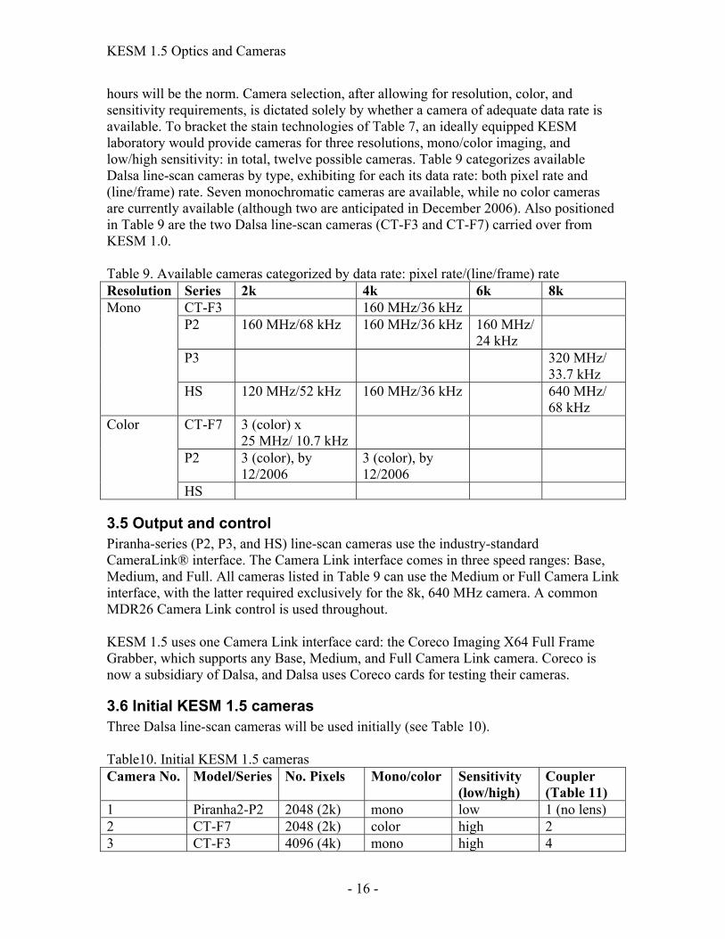
hours will be the norm. Camera selection, after allowing for resolution, color, and sensitivity requirements, is dictated solely by whether a camera of adequate data rate is available. To bracket the stain technologies of Table 7, an ideally equipped KESM laboratory would provide cameras for three resolutions, mono/color imaging, and low/high sensitivity: in total, twelve possible cameras. Table 9 categorizes available Dalsa line-scan cameras by type, exhibiting for each its data rate: both pixel rate and (line/frame) rate. Seven monochromatic cameras are available, while no color cameras are currently available (although two are anticipated in December 2006). Also positioned in Table 9 are the two Dalsa line-scan cameras (CT-F3 and CT-F7) carried over from KESM 1.0. Table 9. Available cameras categorized by data rate: pixel rate/(line/frame) rate Resolution Series 2k 4k 6k 8k

CT-F3 160 MHz/36 kHz P2 160 MHz/68 kHz 160 MHz/36 kHz 160 MHz/

24 kHz

P3 320 MHz/ 33.7 kHz

Mono

HS 120 MHz/52 kHz 160 MHz/36 kHz 640 MHz/ 68 kHz

CT-F7 3 (color) x 25 MHz/ 10.7 kHz

P2 3 (color), by 12/2006

3 (color), by 12/2006

Color

HS

3.5 Output and control Piranha-series (P2, P3, and HS) line-scan cameras use the industry-standard CameraLink® interface. The Camera Link interface comes in three speed ranges: Base, Medium, and Full. All cameras listed in Table 9 can use the Medium or Full Camera Link interface, with the latter required exclusively for the 8k, 640 MHz camera. A common MDR26 Camera Link control is used throughout. KESM 1.5 uses one Camera Link interface card: the Coreco Imaging X64 Full Frame Grabber, which supports any Base, Medium, and Full Camera Link camera. Coreco is now a subsidiary of Dalsa, and Dalsa uses Coreco cards for testing their cameras.

3.6 Initial KESM 1.5 cameras Three Dalsa line-scan cameras will be used initially (see Table 10). Table10. Initial KESM 1.5 cameras Camera No. Model/Series No. Pixels Mono/color Sensitivity

(low/high) Coupler (Table 11)

1 Piranha2-P2 2048 (2k) mono low 1 (no lens) 2 CT-F7 2048 (2k) color high 2 3 CT-F3 4096 (4k) mono high 4


- 17 -

Camera 1, the new Piranha2 P2-2k camera, uses a 10µm pixel size. For Zeiss optics its sensor just covers the 20mm diameter field of view in the intermediate image plane. Direct (no lens) optics is used to couple between the tube lens and camera, giving the best image quality possible. No higher pixel count is meaningful for the 63X objectives, as determined by the Rayleigh optical resolution criterion and Nyquest sampling (see Table 5 above). Cameras 2 and 3 are being carried over from KESM 1.0. These cameras, the Dalsa CT-F7 and CT-F3 cameras respectively, are more than 5 years old, a generation ago in the fast-moving digital camera world. Neither camera is currently manufactured by Dalsa. These cameras were designated at the time of purchase as high-sensitivity cameras (i.e., having multiple TDI registers). Today these older cameras (when operated at 32-TDI registers, our normal operating point) have lower responsivity than the new, single-line, Piranha2-series cameras (e.g., Camera 1 in Table 10). Both older cameras will be phased out, and replaced by newer Dalsa cameras drawn from Table 9, when funds become available.

4. Line-Scan Camera Couplers The minimum number of optical couplers required to match the KESM 1.5 microscope to all applicable Dalsa Piranha-series line-scan cameras is determined in Sec. 4.1 and 4.2 below (see Table 11). We show that four couplers in total are required (Tables 11 and 12). Coupler one uses 1X (no lens) direct imaging of the intermediate image plane, and will be used with the Piranha 2k (10µm pixel) camera for high-resolution imaging with the Zeiss 63X objective and low-resolution imaging with the Olympus Super 20X objective. Couplers 2 and 4 are used with the CT-F7 and CT-F3 cameras, respectively. Furthermore, all cameras for a given coupler use a common mount (M42 x 1 for couplers 1 and 2 and M72 x 0.75 for couplers 3 and 4). All cameras use a common computer interface card (Coreco Imaging X64 Full Frame Grabber, see Sec. 3.5). The line-scan camera couplers used in KESM 1.5 are summarized in Sec. 4.3.

4.1 Grouping line-scan cameras by coupler Available Dalsa Piranha-series cameras and our older CT-series cameras used by KESM 1.0 (see Table 9 above) are sorted by increasing sensor diameter in Table 11. Cameras are then partitioned by sensor diameter into four groups, each group using a common coupler. As shown in Table 11, all cameras for a given coupler can use a common mount, either the M42 x 1 mount for smaller-format cameras or the M72 x 0.75 mount for larger-format cameras. Table 12 summarizes the coupler specifications. Table 11. Available cameras listed by increasing sensor diameter Coupler Camera No.

Pixels Pixel Size (µm)

Sensor Dia. (mm)

Lens Mounts

Output (Camera Link)

Olympus Reso-lution9

Zeiss Reso-lution3

1 Piranha2 P2

2k 10 20.48 C, F, M42

M LR HR

2 Piranha2 HS

2k 13 26.62 F, M42 M LR HR


- 18 -

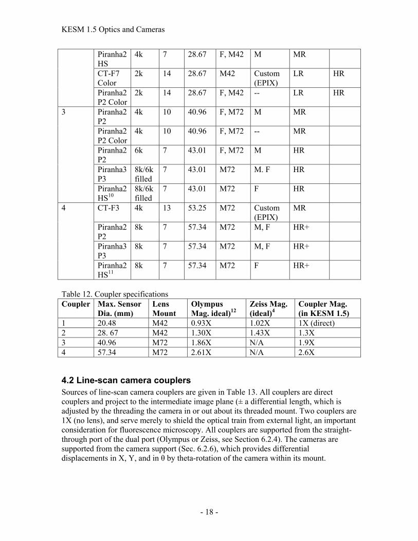
Table 12. Coupler specifications Coupler Max. Sensor

Dia. (mm) Lens Mount

Olympus Mag. ideal)12

Zeiss Mag. (ideal)4

Coupler Mag. (in KESM 1.5)

1 20.48 M42 0.93X 1.02X 1X (direct) 2 28. 67 M42 1.30X 1.43X 1.3X 3 40.96 M72 1.86X N/A 1.9X 4 57.34 M72 2.61X N/A 2.6X

4.2 Line-scan camera couplers Sources of line-scan camera couplers are given in Table 13. All couplers are direct couplers and project to the intermediate image plane (± a differential length, which is adjusted by the threading the camera in or out about its threaded mount. Two couplers are 1X (no lens), and serve merely to shield the optical train from external light, an important consideration for fluorescence microscopy. All couplers are supported from the straight-through port of the dual port (Olympus or Zeiss, see Section 6.2.4). The cameras are supported from the camera support (Sec. 6.2.6), which provides differential displacements in X, Y, and in θ by theta-rotation of the camera within its mount.

Piranha2 HS

4k 7 28.67 F, M42 M MR

CT-F7 Color

2k 14 28.67 M42 Custom (EPIX)

LR HR

Piranha2 P2 Color

2k 14 28.67 F, M42 -- LR HR

Piranha2 P2

4k 10 40.96 F, M72 M MR

Piranha2 P2 Color

4k 10 40.96 F, M72 -- MR

Piranha2 P2

6k 7 43.01 F, M72 M HR

Piranha3 P3

8k/6k filled

7 43.01 M72 M. F HR

3

Piranha2 HS10

8k/6k filled

7 43.01 M72 F HR

CT-F3 4k 13 53.25 M72 Custom (EPIX)

MR

Piranha2 P2

8k 7 57.34 M72 M, F HR+

Piranha3 P3

8k 7 57.34 M72 M, F HR+

4

Piranha2 HS11

8k 7 57.34 M72 F HR+


- 19 -

Table 13. Line-scan camera couplers used in KESM 1.5 Optics Magnification Source Part No.

1X (no lens) Olympus U-TV1X, U-TMAD

1.3X Quioptic DT13OU 1.9X Quioptic DT19OU

Olympus

2.6X From KESM 1.0 1X (no lens) Micro Star Tech. Zeiss 1.3X Quioptic (custom) DT13ZZ

5. Observation Camera and its Coupler 5.1 Uses of the observation camera The KESM 1.5 microscope does not have binoculars or a trinocular. The field of view in the specimen plane is imaged via a digital observation camera, which under program control can run in either still or video mode. The observation camera will be used for coarse focusing, microscope/knife alignment, and ribbon monitoring. Ribbon monitoring entails examining the top facet of the knife at the end of each stroke for residual sectioning debris remaining after the knife has been flushed. Automation of knife/optical alignment and ribbon monitoring require taking digital images of the top facet of the knife. An area-scan digital camera has been chosen for this purpose.

5.2 Choice of the observation camera An IEEE-1394/FireWire CMOS digital color camera (PixeLINK PL-A742, 1280 x 1024 pixels) has been selected as the observation camera (Table 14). Table 14. Observation camera parameters Imaging Device CMOS Sensor (2/3” Chip) Manufacturer and Model PixeLINK PL-A742 CMOS color camera Video Output IEEE-1394/FireWire Power Requirements Via IEEE.a cable Lens Mount C-Mount Synchronization External via trigger Control Via downloadable software Output Image Size Range (H x V) 1280 x 1024

5.3 Couplers for the observation camera The observation camera images the entire field of view of the microscope. The knife edge and the newly-cut tissue ribbon, illuminated by a structured light stripe across the top facet of the knife, are visible on the computer monitor. Unlike conventional video couplers, which match the chip diagonal to the field number (FN) of the microscope, the coupler for the observation camera matches the horizontal width of the chip to FN. This results in couplers of low magnification:

Chip horizontal size/FN (Olympus) = 8.6mm/22mm = 0.39X


- 20 -

Chip horizontal size/FN (Zeiss) = 8.6mm/20mm = 0.43X Slightly less magnification is acceptable. Both couplers (Table 15) use a C-mount to attach to the camera. Each coupler mounts to its own dual port containing a beam-splitting dichromatic mirror. Table 15. Couplers for the observation camera Optics Magnification Manufacturer Part Number(s) Olympus 0.38X Qioptic DC38NN13 Zeiss 0.38X Qioptic DC38NN

6. Knife/Microscope/Camera Mounting In this section we position and orient the knife and microscope/camera relative to the mounting backplane fastened to the granite bridge behind the stage and parallel to the X-Z plane defined by the three-dimensional stage. The basic framework, a three-dimensional Cartesian coordinate system defined by the knife/microscope axes when perfectly aligned, is introduced in Sec. 6.1. Into this framework the components of the optical train are introduced in stack order, from objective to camera (Sec. 6.2). The knife assembly components are then introduced in Sec.6.3. This section also explains the trade-off between knife and the microscope/camera adjustments, which makes it possible to bring these two assemblies into proper alignment. The specimen tank (Sec. 6.4) sits atop the 3-axis precision stage. Its structure and allowable displacements are tightly constrained by the prior optical and knife component mountings.

6.1. Knife/microscope axes define a 3D Cartesian coordinate system The microscope/camera scans the specimen ribbon as it rolls across the top facet of the diamond knife, imaging an illuminated stripe parallel to the knife edge and displaced by 10-20µm from the knife edge (Fig. 2). Upon proper alignment, the specimen plane of the microscope coincides with the top facet of the knife. Fig. 4. Knife/microscope axes

define 3D Cartesian coordinate system (Y’-axis parallel Y-axis)


- 21 -

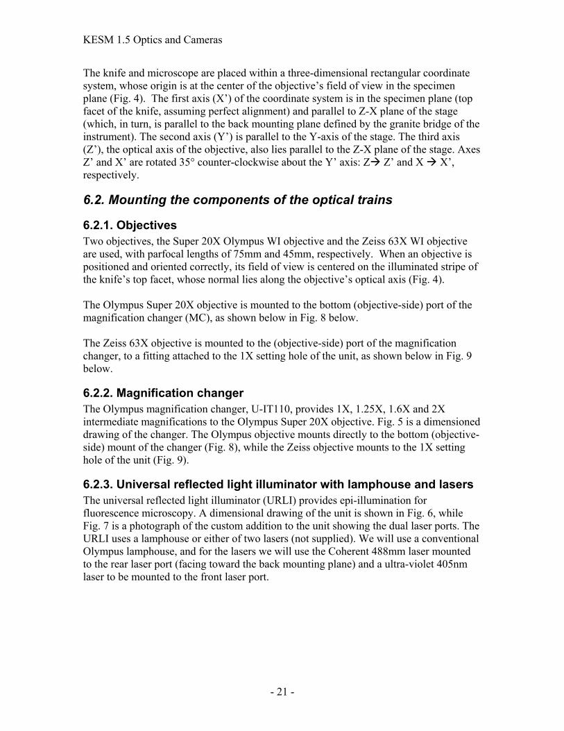
The knife and microscope are placed within a three-dimensional rectangular coordinate system, whose origin is at the center of the objective’s field of view in the specimen plane (Fig. 4). The first axis (X’) of the coordinate system is in the specimen plane (top facet of the knife, assuming perfect alignment) and parallel to Z-X plane of the stage (which, in turn, is parallel to the back mounting plane defined by the granite bridge of the instrument). The second axis (Y’) is parallel to the Y-axis of the stage. The third axis (Z’), the optical axis of the objective, also lies parallel to the Z-X plane of the stage. Axes Z’ and X’ are rotated 35° counter-clockwise about the Y’ axis: Z Z’ and X X’, respectively.

6.2. Mounting the components of the optical trains

6.2.1. Objectives Two objectives, the Super 20X Olympus WI objective and the Zeiss 63X WI objective are used, with parfocal lengths of 75mm and 45mm, respectively. When an objective is positioned and oriented correctly, its field of view is centered on the illuminated stripe of the knife’s top facet, whose normal lies along the objective’s optical axis (Fig. 4). The Olympus Super 20X objective is mounted to the bottom (objective-side) port of the magnification changer (MC), as shown below in Fig. 8 below. The Zeiss 63X objective is mounted to the (objective-side) port of the magnification changer, to a fitting attached to the 1X setting hole of the unit, as shown below in Fig. 9 below.

6.2.2. Magnification changer The Olympus magnification changer, U-IT110, provides 1X, 1.25X, 1.6X and 2X intermediate magnifications to the Olympus Super 20X objective. Fig. 5 is a dimensioned drawing of the changer. The Olympus objective mounts directly to the bottom (objective-side) mount of the changer (Fig. 8), while the Zeiss objective mounts to the 1X setting hole of the unit (Fig. 9).

6.2.3. Universal reflected light illuminator with lamphouse and lasers The universal reflected light illuminator (URLI) provides epi-illumination for fluorescence microscopy. A dimensional drawing of the unit is shown in Fig. 6, while Fig. 7 is a photograph of the custom addition to the unit showing the dual laser ports. The URLI uses a lamphouse or either of two lasers (not supplied). We will use a conventional Olympus lamphouse, and for the lasers we will use the Coherent 488mm laser mounted to the rear laser port (facing toward the back mounting plane) and a ultra-violet 405nm laser to be mounted to the front laser port.


- 22 -

Fig. 5. Magnification Changer


- 23 -

Fig. 6. Universal reflected light illuminator (URLI)

Fig. 7. Modified URLI with dual laser ports


- 24 -

Because the distance from the optical axis to its rear port considerably exceeds the corresponding distance in the Nikon URLI used in KESM 1.0, the Olympus URLI is mounted sideways, with its controls facing up and to the right, while its long axis extends down and to the left (Figs. 8 and 9). The lamphouse is beyond the limited travel of stage during sectioning/scanning. The unit, in common with the camera mount support, is attached to the Y’-axis linear stage by thick rectangular stock (Figs. 8 and 9). Amply space is left between the back mounting plane and the URLI, when the URLI is mounted as shown in Figs. 8 and 9. All cantilevered parts in KESM 1.0 can be shorted accordingly, and the specimen tank positioned more centrally over the Aerotech lift stage. Limiting this foreshortening are three constraints: (1) clearance for the observation camera, (2) clearance for the rear-mounted laser (Coherent 488nm), and (3) maintaining a ±25mm displacement for the specimen mount from it center position.

6.2.4. Dual port with tube lenses (Olympus and Zeiss) The dual port is mounted atop the URLI via its male Olympus fitting. The dual port consists of three parts: the beam splitter (BS) and two tube lens units (TLUs) inserted into its straight and side ports (Fig. 10). The BS contains a dichroic mirror and feeds 33% of the light to the side port, and hence to the observation camera via its coupler. Two dual ports are used in KESM 1.5: one each for Olympus and Zeiss optics, respectively. They are distinguished only by the TLUs inserted into the two ports: each port holds a tube lens unit (TLU) for the appropriate optics (Table 16). The TLUs are designed to be parfocal with the intermediate image plane: that is, the tube lens in mounted in the TLU such that the distance from the shoulder of the TLU to the intermediate image plane is independent whether an Olympus or Zeiss tube lens is embedded in the TLU. Critical to the design of the dual port is one overriding consideration: to minimize its usage of ∞-space -- to get this distance down to 38mm or less. Only then can the 170mm upper bound on ∞-space for Olympus optics be met; the ∞-space constraint for Zeiss optics is equally severe.

Fig. 8. Mounting of Olympus Super 20X objective to the magnification changer (MC) and universal reflected light illuminator (URLI)

Fig. 9. Mounting of Zeiss 63X objective to the magnification changer (MC) and universal reflected light illuminator (URLI)


- 25 -

Table 16. Dual port tube lenses Olympus/Zeiss Optics Straight port tube lens Side port tube lens Olympus tube port U-TLU U-TLU Zeiss tube port Zeiss 130mm tube lens in

TLU tube mounting Zeiss 130mm tube lens in TLU tube mounting

6.2.5. Observation camera and couplers The observation camera coupler extends from the side port of the dual port (Olympus or Zeiss). The observation camera couplers are optics-dependent: different couplers are used for Olympus and Zeiss optics (Table 14, Sec. 5.3), though physically they are almost indistinguishable. The double doublet optics is displaced slightly between the two units to insure that their image planes are parfocal with the camera sensor chip.

Fig. 10. Dual port (side view)


- 26 -

The coupler to the observation camera can not intrude below the shoulder of the dual port, and into space occupied by the URLI. The use of a coupler, stripped of its outer housing, and only 32mm in diameter makes this possible. A PixeLINK PL-A742-R color camera has been selected as the observation camera (Sec. 5.2). This camera uses a right-angle configuration to shorten its outreach from the side port of the dual port (Fig. 11).

6.2.6. Line-scan camera couplers The line-scan camera couplers (Table 13) mount to the straight-through port of the dual port. As described in Section 4.2, these couplers do not directly support the cameras, as the camera support allows differential movements in the X, Y, and θ to accommodate microscope/knife misalignment.

6.2.7. Line-scan cameras and their mounting The camera mounting in KESM 1.0 has worked well; it will be little changed in KESM 1.5, except in four minor regards: (1) The camera mount support, in common with the URLI, will be attached to the manually-positioned Y’-axis linear stage (Figure 4); (2) the camera mount support can be shortened (less cantilevering) in view of the sideways mounting of the URLI; (3) finer threads will be used for differential X, Y, and θ displacements (Fig. 12), and (4) a M42 x 1 camera mount for small format cameras (coupler classes 1 and 2, Table 11) will be provided, in addition to the M72 x 0.75

Fig.11. Observation camera and coupler


- 27 -

camera mount for larger format cameras (coupler classes 3 and 4, Table 11) The latter was used in KESM 1.0. An adapter ring (72 x 0.75 to M42 x 1) can be used to down-size the M72-mount to the M42-mount.

6.3. Knife assembly components and adjustments

6.3.1. Diamond knife and knife module The diamond knife and knife module has undergone a number of transformations in KESM 1.0. The major change in KESM 1.5 is reducing the facet angle of the knife to 30°, leaving a clearance angle of 5° between the bottom facet of the knife and the newly-cut surface of the block (Fig. 1). Three additional, if less consequential, changes are: (1) providing a more substantial mounting of the knife module to the knife adjustment assembly; (2) enhancing ribbon extraction by moving the water (and ribbon) orifice closer to the top facet of the knife; and (3) welding the knife to its mount using a precision fixture that insures that the top facet of the knife will be at 35° above the horizontal when installed in the instrument (see Sec. 6.3.2 below).

6.3.2. Knife mounting and adjustments The microscope defines a rectangular coordinate system by its optical axis, its specimen plane, and a line parallel to the Y-axis of the stage (Fig. 4). The microscope, and hence its coordinate system is given only one degree of freedom: a focusing adjustment, which moves the components of the optical train and attached camera along its optical axis. The knife must be positioned and oriented relative to this microscope-defined coordinate system. Perfect alignment would require that the knife edge (1) lie in the specimen plane, (2) centered in the field of view, and (3) oriented such that its image is aligned with the linear sensor of the camera. Rigid motion of the knife to attain perfect alignment would requires, like for any rigid body, six degrees of freedom (dof). Knife adjustments, however, must be minimized and kept extremely rigid to minimize the potential for chatter during sectioning. Therefore, of the six degrees of freedom, the knife is assigned only three and the remaining three degrees of freedom are compensated by differential translation and rotation of the camera. Conceptualizing the knife as a rowboat, the knife is assigned one translational dof (focusing-like displacement along the X’ axis, see Fig. 4), and two orientation degrees of freedom: roll and yaw (Fig. 12). Pitch is adjusted at the time of manufacture of the knife module: the diamond knife is placed in a custom jig, and welded to the knife module. In summary, the three degrees of freedom not provided the knife are compensated by incorporating three dof’s in the adjustments provided by the camera mounting.

6.3.3. Ribbon extractor and pump The problems with the prototype ribbon extractor are well-known. These stem from multiple sources: (1) Extraction suction upon the newly-cut ribbon is inadequate, leading to ribbon fold-over, which in turn gives rise to occasional vertical blobs in the scanned image; (2) Occasional debris ca be left attached to the top facet of the knife at the end of the sectioning stroke. This debris will be removed by an end-of-stroke flush, and validated as clean by an automated inspection using the observation camera.


- 28 -

The pump assembly was upgraded during KESM 1.0 to a larger size. Mounting the pump to the frame of the instrument does not appear to introduce significant vibration; no difference in degree of chatter was observed when cutting with the pump turned off.

6.4. Specimen tank

6.4.1 Specimen tank The specimen tank, mounted atop the three axis stage, carries the specimen under water. The specimen tank with its spill tray has worked well. The principal improvements in KESM 1.5 are: (1) Lighten the specimen tank (including water fill), as both the specimen tray and the Y-axis stage rest atop the lift stage, and nearly exceed its load limit; (2) Move the specimen tank back toward the rear mounting plate so as to reduce the extent of cantilevering required.

6.4.2. Specimen ring The specimen is mounted to a specimen ring (Fig.2a), which is keyed to the bottom of the specimen tank. The specimen ring, introduced in KESM 1.0, has worked well. Its home position is with the microscope/knife centered over the specimen block, prior to sectioning, and the lift stage at its lowest position. The lift stage raises as serial sections are taken. Presently mouse brains are embedded apart from the specimen ring, using a minimum of plastic embedding compound, and then in a second stage, mounted atop the plastic-filled specimen ring. As work expands with rat brain, which are four times larger in volume

Fig. 12. Adjustment of knife orientation


- 29 -

than the mouse brain, it may prove necessary to introduce a larger specimen ring, but that decision would be premature today.

6.4.3. Extraction of knife/microscope from specimen tank First, the specimen tank is returned to its home position prior to this movement. The knife is then extracted from the specimen tank as follows: the manual knife stage is unlocked and retracted along the X’ axis (Fig. 4). Likewise, the microscope manual stage is unlocked and retracted along the Y’-axis (Fig.4).

6.4.4. Constrained movement of tank The sidewise mounting of the URLI and its associated lamphouse constrains free movement of the specimen tank. However, as seen in Figs. 8 and 9, there is adequate room for the 15mm-20mm travel required for sectioning.

Appendix A. Dalsa Line-Scan Cameras Truncated data sheet information on select Dalsa line-scan cameras is tabulated below. Data sheets for currently available cameras, including CAD mechanical drawings and mounting details, can be downloaded from the Dalsa website: http://www.dalsa.com. The prototype instrument, KESM 1.0, uses two high-sensitivity line-scan cameras: CT-F7 (color, 2k) and CT-F3 (mono, 4k); for details see Sec. A.1. The Piranha2 series of line-scan cameras (both the P2-series, single-register cameras and the high sensitivity HS-series, multiple TDI register cameras) are described in Sections A.2 and A.3 respectively. In particular, the 2048-pixel Prianha2 camera, P2 40-2k, used in KESM 1.5, is described there. New Pyranha2 color line-scan cameras, anticipated December 2006 but not yet announced by Dalsa, are described briefly in Sec. A.4. Finally, Sec. A.5 describes the recently announced Piranha P3-series line-scan cameras. These latter cameras, though not directly applicable to KESM 1.5, give insight into the probable technological direction of future Dalsa line-scan cameras, and show the impact of such manufacturing applications as the testing of large-format LCD panels.

A.1. First-generation KESM cameras The Dalsa high-sensitivity line-scan cameras, (CT-F7, (2k, color) and CT-F3 (4k, mono) are used with the prototype KESM 1.0.. Neither camera is currently manufactured by Dalsa. Table A.1 describes their imaging characteristics. Table A.1. CT-series cameras used in KESM 1.0 Resolution 2048 x 64 TDI Color 4096 x 96 TDI Camera Model CT-F7 CT-F3 Data Rate 3 (color) x 25 MHz 4 x 40 MHz Max. Line/Frame Rate 10.7 kHz 36 kHz Pixel Size 14µm 13 µm Data Format 8 bit 8 bit Output Custom Custom Lens Mount M72 x 0.75 M72 x 0.75


- 30 -

Responsivity DN/(nJ/cm2) 180 DN/(nJ/cm2)/ 60 DN/(nJ/cm2)/ for 32 TDI

Sensor Aperture 28.7 x 1.6mm 53.3 x 1.3mm Control EPIX card/software EPIX card/software

A.2. Piranha2 P2-series line-scan cameras Table A.2. Piranha2 P2-series cameras Resolution 2048 4096 6144 Data Rate 4 x 40 MHz 4 x 40 MHz 4 x 40 MHz Max. Line/Frame Rate 68 kHz 36 kHz 24 kHz Pixel Size 10µm 10µm 7µm Data Format 8, 10 bit 8, 10 bit 8, 10 bit Output Medium Camera

Link Medium Camera Link

Medium Camera Link

Lens Mount C, F, M42 x 1 mount

F, M72 x 0.75 mount

F, M72 x 0.75 mount

Responsivity 76 DN/(nJ/cm2) @ 10dB

76 DN/(nJ/cm2) @ 10dB

38 DN/(nJ/cm2) @ 10dB

Control MDR26 Camera Link

MDR26 Camera Link

MDR26 Camera Link

Cost (USD) $4651 $5481 $5880

A.3. Piranha3 P3-series line-scan cameras Table A.3. Piranha3 P3-series cameras Resolution 8192 12288 Data Rate 8 x 40 MHz 8 x 40 MHz Max. Line/Frame Rate 33.7 kHz 23.5 kHz Pixel Size 7µm 5 µm Data Format 8,12 bit 8, 12 bit Output Med, Full Camera

Link Med, Full Camera Link

Lens Mount M72 x 0.75 M72 x 0.75 Responsivity 44 DN/(nJ/cm2) 27 DN/(nJ/cm2) Control MDR26 Camera Link MDR26 Camera Link Cost (USD) $6185

A.4. Piranha2 HS-series line-scan cameras Table A.4. Piranha2 HS-series cameras Resolution 2048 x 64 TDI 4096 x 96 TDI 8192 x 96 TDI Data rate 2 x 60/4 x 30 MHz 4 x 40 MHz 320/640 MHz Max. Line/Frame Rate

52 kHz 36 kHz 34/68 kHz

Pixel Size 13µm 7 µm 7µm


- 31 -

Data Format 8,10 bit 8,12 bit 8,10 bit Output Base, Medium

Camera Link Base, Medium Camera Link

Medium, Full Camera Link

Lens Mount M42 x1, F mount M42 x 1, F mount M72 x 0.75 Responsivity 1610 DN/(nJ/cm2) 1170 DN/(nJ/cm2) 1170 DN/(nJ/cm2) Control MDR26 Camera

Link MDR26 Camera Link

MDR26 Camera Link

Cost (USD) $5942 $10,880/$14,048

A.5. New Piranha2 color line-scan cameras Table A.5. New Piranha2 color cameras (anticipated December 2006, preliminary data) Resolution 2048 4096 Pixel Size 14µm 10µm

Appendix B. Comparison of Microscopes for Brightfield and Fluorescence Imaging Table B.1 gives a comparative study of four microscope systems: (1) the Olympus BX51-WI+DPMC, (2) the Olympus BX51+ BX-RFA, (3) the Zeiss Axio Imager, and (4) the Nikon Eclipse PhysioStation E600FN. The later microscope was used in KESM 1.0. The data in the table was derived from the four corresponding schematics (Fig. 17). Table B.1. Comparative study of four microscope systems Dimensions (mm) Olympus

BX51+WI +DPMC

Olympus BX51+BX -RFA

Zeiss Axio Imager

Nikon Eclipse E600FN

Objective Olympus Super 20X

Zeiss 63X Nikon 10X & 40X

Parfocal length 75 45 45 60 Specimen plane to mid-plane URLI

153.9 126 187.5

e∞-space to trinocular 134 124 128 155 Trinocular height 90.8 62.5 >86.7 82.7 URLI height (L) 87.5 87.5 55 URLI width (max) (W) 88 88 URLI length: optical axis to rear port (L1)

261 261 327.6 235

knife-edge scanning microscope (kesm 1.5): optics …department of computer science texas a&m...

Documents