journal of gas technology, jgt
TRANSCRIPT


Journal of Gas Technology, JGT
Editorial DirectorMohammadreza Omidkhah
Editor-in-ChiefAli Vatani
Associate EditorAbolfazl Mokhtari
Managing EditorMohamad Reza Jafari Nasr
Editorial Board MembersAli Vatani, University of Tehran
Mohammadreza Omidkhah, Tarbiat Modares UniversityVahid Taghikhani, Sharif University of Technology
Bahman Tohidi, Heriot-Watt UniversityMohammad Jamialahmadi, Petroleum University of Technology
Riyaz Kharrat, Petroleum University of TechnologyRahbar Rahimi, University of Sistan and Baluchestan
Masoud Soroush, Drexel UniversityMojtaba Shariati Niasar, University of Tehran
Seyed Reza Shadizadeh, Petroleum University of TechnologyMajid Abedinzadegan Abdi, Memorial University of Newfoundland
Hossein Golshan, TransCanada Co.Toraj Mohammadi, Iran University of Science and Technology
Reza Mosayebi Behbahani, Petroleum University of TechnologyMahmood Moshfeghian, Oklahoma State University
Seyed Hesam Najibi, Petroleum University of Technology
Technical EditorMohamad Reza Jafari Nasr
LayoutHamidreza karimi
Cover DesignHamidreza karimi
Contact InformationIranian Gas Institute:
http://www.jgt.irangi.orgJournal Email Address:
ISSN: 2588-5596
Volume 6. February 2020

Table of Contents
Simulation and Thermodynamic Analysis of a Closed Cycle Nitrogen Expansion Process for Liquefaction of Natural Gas in Mini-scale
...................................................... 4
Amirhossein Yazdaninia, Ali Vatani, Marzieh Zare, Mojgan Abbasi
Aspen Plus Simulation of Power Generation Using Turboexpanders in Natural Gas Pressure Reduction Stations
...................................................... 14
Bijan Hejazi, Fatollah Farhadi
Simulation of an Industrial Three Phase Boot Separator Using Computational Fluid Dynamics
...................................................... 30
Zohreh Khalifat, Mortaza Zivdar, Rahbar Rahimi
Optimizing CO2/CH
4 Separation Performance of Modified
Thin Film Composite Pebax MH 1657 Membrane Using a Statistical Experimental Design Technique
...................................................... 43
Tayebeh Khosravi
Strategic Storages of Gas in Salt Layers and Creep and Overburden Effects on Volume Loss
...................................................... 51
Alireza Soltani, Hassan Mirzabozorg
Risk Based Inspection of Composite Components in Oil and Gas Industry
...................................................... 60
Meysam Najafi Ershadi, Mehdi Eskandarzade, Ali Kalaki

4 Journal of Gas Technology . JGT
Simulation and Thermodynamic Analysis of a Closed Cycle Nitrogen Expansion Process for Liquefaction of Natural Gas in Mini-scale
• Amirhossein Yazdaninia1, Ali Vatani1*, Marzieh Zare2, Mojgan Abbasi3
1. Institute of Liquefied Natural Gas (ILNG), School of Chemical Engineering, College of
Engineering, University of Tehran, Tehran, Iran.
2. National Iranian Gas Company (NIGC), Tehran, Iran.
3. Institute of Petroleum Engineering, School of Chemical Engineering, College of Engineering,
University of Tehran, Tehran, Iran.
Corresponding author Email address: [email protected]
Received: June 18, 2019 / Accepted: August 27, 2019ـــــــــــــــــــAbstract
In this study a closed nitrogen expansion cycle (Niche) has been simulated with Aspen HYSYS V8.4.
Energy and exergy analysis were applied to evaluate the process. Results of energy analysis indicated
that specific power consumption of this process is 0.68 kWh/kg LNG. The results of exergy analysis
showed that exergy efficiency of Niche LNG is 35.51%. It is concluded there is an interaction between
specific power consumption and exergetic efficiency. Moreover, the highest value of exergetic
efficiency and irrevsibility belong to compressor (C3) and gas turbine (E1). Moreover, this process can
be suitable for mini-scale LNG plants.
Keywords: Closed nitrogen expansion Cycle, Exergy Analysis, Specific power consumption, LNG.

5Volume 6 / Issue 1 / February 2020
ــــــــــــــــــــــــــــــــــ1. Introduction
Among the methods exist for transportation of natural gas, liquefaction of natural gas is the most economical and simple because the occupied volume of liquefied natural gas is 600 times less than natural gas by cooling down it up to -162 °C at 1 bar. Basically, energy consumption of natural gas liquefaction processes shouldn’t be more than a specified value because it won’t be economical [1]. As well as, LNG demand is increasing about 6% every year [2]. For this purpose, some companies such as Mustang, ABB Lummus Global Inc. and Gasconsult improved the LNG processes through designing new heat exchangers or process configurations to reduce the energy consumption.
Totally, main refrigeration cycles for LNG production can be classified into three groups including: Cascade, Mixed refrigerant and Expansion cycles [3,4]. Generally, the Cascade processes, propane precooling mixed refrigerant (C3MR) and dual mixed refrigerant (DMR) cycles, are used for the base-load scales and the single mixed refrigerant (SMR) and nitrogen expansion cycles mainly used for the small scale LNG plants which have been compared in the different references [5,6,7,8]. Normally, SMR processes have higher efficiency compared with N
2-
expansion cycles, but N2 cycles are more simple
and more safe processes [9,10].
There are several processes for liquefaction of natural gas with nitrogen expansion cycles such as OCX-R, NDX-1, OCX-2, Niche LNG, ZR LNG [10,11,12,13]. The most important parameter in all of these processes is energy consumption which can be calculated via energy analysis. With exergy analysis it will be determined where and how much energy is wasting through process [14]. Furthermore, an exergy analysis usually identifies which equipment have the maximum performance in the process and have the highest lost work [15].
Many investigations have been done for liquefaction of natural gas with Nitrogen expansion cycles which used thermodynamic
analysis (energy and exergy) to investigate the performance of the processes. Remeljej and Hoadley [4] investigated four processes including single-stage mixed refrigerant (SMR), a two-stage expander nitrogen refrigerant and two open-loop expander processes in the steady state. They found that energy consumption of the SMR process is less than the other ones. However, nitrogen refrigerant process and the New LNG open-loop process are suitable for offshore compact LNG production. Yoan et al. [16] recommended a single stage nitrogen expansion process with carbon dioxide pre-cooling cycle for small scale LNG plants, then compared with propane pre-cooling, N
2-
CH4 expander cycle process and new mixed
refrigeration cycle proposed by Cao et al. [6]. They concluded that this process is suitable for small scale LNG plants due to safe operation. He and Ju. [17] added two different precooling cycles including propane and R410a as a refrigerant to a nitrogen expansion liquefaction process to improve its performance. The results showed that the energy consumption for the nitrogen expansion process with R410a and propane reduced by 22.74% and 20.02% respectively, compared to the nitrogen expansion process without precooling. He and Ju [18] proposed a parallel nitrogen expansion liquefaction process for small scale plants in a skid mounted package. They showed that the energy consumption of the process is reduced approximately 4.69% compared to the conventional nitrogen expansion processes. Moein et al. [19] investigated the effect of the methane addition on a dual nitrogen expansion cycles for LNG production. They concluded that the work consumption of the process will be minimized when the concentration of the methane in the refrigerant is equal to 26 ± 1 mol% in which the net required work of the process is 8% less compared to the optimized case of the process with pure nitrogen as a refrigerant. Palizdar et al [20] applied energy, conventional, and advanced exergy analysis to three mini scale nitrogen expansion for LNG production including: APN, Statoil and

6 Journal of Gas Technology . JGT
BHP Nitrogen expansion process. Results of conventional exergy analysis indicated that air coolers have a high irreversibility and have a small exergy efficiency. Also, results of energy analysis showed that APN process has the least energy consumption compared with other processes (approximately 85%). Results of advanced exergy analysis showed that for all of these processes, exergy destruction of the air coolers is unavoidable. Furthermore, a high portion of total avoidable exergy destruction of the processes (up to 85%) belongs to compressors and expanders.
However, among the works have been done for LNG production with expansion processes and some of them were mentioned in above, there are several nitrogen expansion processes that have not been investigated yet, such as open and closed nitrogen expansion cycle processes. In this study, a closed nitrogen expansion cycle (Niche) has been simulated. The studied process is invented by ABB Lummus Global Inc company [21]. Then, thermodynamic analysis was applied to this process including energy and exergy analysis. In energy analysis some parameters such as SPC and COP will be calculated and T-s and P-h diagrams are plotted. Moreover, in exergy analysis it is determined which equipment has the highest exergetic efficiency and irreversibility.
ــــــــــــــــــــــــــــــــــــــــــــــــــ2. Process Description
The process flow diagram has been illustrated in Figure 1, schematically. As shown, the process consists of two independent refrigerant cycles. The first cycle uses methane as refrigerant and the second cycle uses nitrogen. The pre-treated natural gas stream (20) at 35 °C and 60 bar enters LNG heat exchanger (75-LNG) and is cooled to -121.54 °C (20-1). The cooled natural gas (20-1) enters LNG heat exchanger (75-1 LNG) and is cooled further to -152.60 °C, approximately (22). The pressure of the cooled natural gas (22) is decreased from 58.75 to 1.35 bar via an expansion valve and its temperature decreases to -161.31 °C (24). The expanded liquefied natural gas (24)
enters a flash tank where LNG and flash gas is separated [21,22].
In the first refrigerant cycle with methane as a refrigerant, expanded methane (44) enters LNG heat exchanger (75-LNG) at -127.10 °C and 6.90 bar and exchanges heat with both inlet natural gas stream (20) and methane refrigerant inlet stream (40), then exits LNG heat exchanger (75-LNG) at 36.86 °C (46). The warmed methane refrigerant (46) is partially compressed in the first compressor (C1) from 6.40 to 21.50 bar and is cooled to 40 °C in the first air cooler (AC1). The partially compressed and cooled methane is then compressed in the second compressor (C2) from 21.40 to 76.53 bar and cooled to 40 °C in the second air cooler (40). Stream 40 is the starting point of the methane refrigerant cycle and enters LNG heat exchanger (75-LNG) at 40 °C and 76.43 bar and cooled in LNG heat exchanger (75-LNG) to -18 °C (42). The cooled methane refrigerant (42) is reduced in pressure by expansion in the expander (E-1) from 75.93 to 6.90 bar and its temperature decreases to -127.10 °C (44). Stream 44 is returned to the LNG heat exchanger (75-LNG) and the cycle is repeated as mentioned above.
In the second refrigerant cycle with nitrogen as the refrigerant, expanded nitrogen (34) at -155 °C and 15bar enters LNG heat exchanger (75-1-LNG) and exchanges heat with precooled natural gas (20-1) and inlet stream of nitrogen refrigerant (30) and exits LNG heat exchanger (75-1-LNG) at 25.58 °C (36). The warmed nitrogen refrigerant (36) is first compressed in the first compressor (C3) from 14.25 to 37.25 bar and cooled to 40 °C in the first air cooler (AC3) then compressed in the second compressor from 37.15 to 80.10 bar and cooled to 40 °C in the second air cooler (AC4). Stream 30 enters LNG heat exchanger (75-1-LNG) at 40 °C and 80 bar, is cooled to -88 °C (32), expanded in expander (E2) from 79.5 to 15 bar and its temperature decreases to -155 °C (stream 34) and the cycle is repeated as mentioned above. Mass flow rate of methane and nitrogen as refrigerant are 1650 kg/hr and 1350 kg/hr, respectively.

7Volume 6 / Issue 1 / February 2020
Table 1. Assumptions of operating and theoretical conditions for the process components
Component Operating conditions Theoretical conditions
Compressor η (%) 75 100
Expander η (%) 75 100
Heat Exchanger ΔTmin (ºC) > 2 0
Air Cooler Pressure drop (bar) 0.1 0
Table 2. Specifications of the feed gas and LNG product streams for Niche LNG process
Feed gas [20] LNG stream
Mass Flow (kg/hr) 470.00 425.40
Temperature (ºC) 35.00 -161.31
Pressure (bar) 60.00 1.35
Molar Enthalpy (kJ/kmol) -73534.18 -89455.00
Components (%mol)
CH4
92.94 94.72
C2H
63.00 3.28
C3H
80.48 0.52
i-C4H
100.06 0.07
n-C4H
100.08 0.09
N2
3.44 1.33
Figure 1. Process flow diagram of Niche LNG process
ــــــــــــــــــــــــــــــ3. Simulation
A closed cycle nitrogen expansion process is simulated by Aspen HYSYS software (V.8.4) in steady state which have been successfully used by the other researchers. The first step and the most important part of the simulation of a process is choosing an accurate property
method. Peng Robinson (PR) equation of state has been selected for simulating of the liquefaction processes which have been previously used and validated for the liquefaction processes [23, 24]. Some assumptions have been applied to simplify the processes which have been mentioned in Table 1. The specifications of feed gas and LNG production streams have been listed in Table 2.

8 Journal of Gas Technology . JGT
The operational conditions of simulated process including temperature, pressure, mass
flow and total exergy for material streams have been illustrated in Table 3.
Table 3. Operational conditions for material streams
Stream name Temperature (oC) Pressure (bar) Mass Flow (kg/h) Total exergy (kW)
20 35 60 470 74.99
20-1 -121.54 59.25 470 112.41
22 -152.58 58.75 470 129.01
24 -161.31 1.35 470 124.48
30 40 80 1350 144.18
32 -88 79.5 1350 159.24
34 -155 15 1350 131.91
36 25.58 14.25 1350 87.63
36-1 149.92 37.25 1350 125.68
36-2 40 37.15 1350 119.09
36-3 141.16 80.1 1350 150.43
40 40 76.43 1650 295.36
42 -18 75.93 1650 299.09
44 -127.1 6.9 1650 200.83
46 36.86 6.4 1650 127.39
46-1 159.43 21.5 1650 236.28
46-2 40 21.4 1650 211.23
46-3 171.58 76.53 1650 324.17
LNG -161.31 1.35 425.4 121.06
V -161.31 1.35 44.6 2.68
ــــــــــــــــــــــــــــــــــــــــــــــــ4. Analysis of Process
4.1. Energy Analysis
Energy analysis of a closed cycle Nitrogen expansion process has been done to calculate the specific power consumption (SPC) and coefficient of performance (COP) of the cycle.
SPC is defined as the total power consumed in the whole process divided by the mass flow rate of the produced LNG [25].
SPC = Total required power in the whole process (kW)
Mass flow rate of LNG (k g h⁄ r)
and COP is defined as:
COP = Total removed heat from natural gas (kW)Total required power in compressors (kW)
Also, deviation of real conditions refrigerant cycles from the ideal state are compared in pressure-enthalpy and temperature-entropy diagrams.
4.2. Exergy analysis
Exergy is defined as the maximum work that obtains from a process [25]. The total exergy rate

9Volume 6 / Issue 1 / February 2020
of the material stream is defined as summation of the potential exergy, kinetic exergy, chemical exergy and physical exergy. Potential and kinetic exergy are negligible in these processes, so total exergy defined as [20]:
ph chE E E= + (1)
( )0 0 0phE H H T S S= − − − (2)
where Ḣ and Ṡ are enthalpy and entropy rates of the stream at initial temperature and pressure and Ḣ0 and Ṡ0 are standard enthalpy and entropy rates of the stream at environment temperature (T0) and pressure. Chemical exergy
(Ėch) is defined as [4]:
0ch
i i i iE x E G x G= + −∑ ∑ (3)
where xi is the mole fraction of ith component in the stream, Ėi
0 is the standard chemical exergy rate of ith component, Ġ is rate of Gibbs free energy of the stream and Ġi is rate of Gibbs free energy of pure ith component at T0 and P0.
After calculating of the total exergy for the material streams, exergy balance must be applied to each component to determine two important parameter in exergy analysis including: exergy efficiency and exergy destruction.
After determining the total exergy of process streams, exergy balance must be written for each component in order to calculate exergy efficiency and exergy destruction. The equations of exergy efficiency and exergy destruction for each component are summarized in Table 4.
Table 4. The equations of exergy efficiency and exergy destruction for each component [20]
ــــــــــــــــــــــــــــــــــــــــــــــــــــــــ5. Results and Discussion
5.1. Energy analysis
Results of energy analysis are shown in table 5, 6, respectively. Specific power consumption of this process (SPC) was calculated 0.68 kWh/kg LNG. This value is approximately close to the literature [26] which confirms almost 0.70 kWh/kg LNG for SPC of dual stage nitrogen expansion processes. In addition, as it can be seen in table 6, pre-cooling cycles coefficient
Table 4. The equations of exergy efficiency and exergy destruction for each component [20]
Component Exergy destruction Exergetic efficiency
Compressor ẆComp- Ėxout + Ėxin (Ėxout - Ėxin) /ẆComp
Expander Ėxin - Ėxout - ẆExp ẆExp /(Ėxin - Ėxout)
Heat exchanger ∑(Ėxin - Ėxout)Cold -∑(Ėxout - Ėxin)Hot ∑(Ėxout - Ėxin)Hot / ∑(Ėxin - Ėxout)Cold
Air Cooler Ėxin - Ėxout -Ėoutair Ėout
air/ (Ėxin - Ėxout)
Total system Summation of irreversibility of all devices ϵ = 1- ( Summation of irreversibility of all devices /∑ ẆComp)
of performance are higher than the other ones due to proximity of hot and cold streams in heat exchanger of these processes the values of COP for nitrogen and methane cycle is 0.42 and 0.19 respectively. Furthermore, the total removed heat from natural gas including latent and sensible heat is 103.60 kW.

10 Journal of Gas Technology . JGT
a
b
Figure 2: T-s diagrams for Niche LNG process a: Methane cycle b: Nitrogen cycle
The temperature - entropy (T-s) and pressure - enthalpy (P-h) diagrams for the ideal and actual
liquefaction cycles are shown in Figures. 2,3. As seen, the deviation of nitrogen cycle is less
than methane cycle.
Table.7 shows the thermodynamic performance of main components of the liquefaction cycles.
a
b
Figure 3: P-h diagrams for Niche LNG process a: Methane cycle b: Nitrogen cycle
Table 5. The value of SPC for liquefaction processes
Niche LNG
Total power consumption in compressors (kW) 365.36
Total produced power in expanders (kW) 75.04
Overall power (kW) 290.32
Mass flow rate of LNG production (kg/h) 425.40
SPC (kWh/kg LNG) 0.68
Table 6. Consumed power, removed heat and coefficient of performance for the cycles
Process Cycle Total required power (kW) Cold duty (kW) COP
Niche LNG Methane 215.75 89.69 0.42
Nitrogen 74.57 13.91 0.19

11Volume 6 / Issue 1 / February 2020
Table 7. Thermodynamic performance of the components
A: Heat exchangers
Component Duty (kW) Min. approach (oC) LMTD (oC)
75-LNG 167.71 3.14 14.16
75-1-LNG 76.40 2.43 12.29
B: Compressors
Component Power consumed (kW) Adiabatic efficiency (%) Pressure ratio Outlet temperature (oC)
C1 134.87 75.00 3.36 159.43
C2 141.32 75.00 3.58 171.58
C3 49.03 75.00 2.61 149.92
C4 40.13 75.00 2.16 141.16
C: Expanders
Component Power produced (kW) Adiabatic efficiency (%) Pressure ratio Outlet temperature (oC)
E1 60.45 75.00 0.09 -127.10
E2 14.59 75.00 0.19 -155.00
Figure 4. indicates composite curves for heat exchangers of Niche LNG process. For all of the air coolers, the specifications of inlet air were considered 25 °C and 1 atm.
a
b
Figure 4. Composite curves of 75- LNG (a) and 75-1- LNG (b) Heat exchangers for Niche LNG process
5.2. Exergy analysis
Figure 5. Results of exergy analysis for
Niche LNG process
Results of exergy analysis have been illustrated in Figure 5. Both of exergy analysis parameters including exergy destruction and exergy efficiency have been calculated with equations of table3. As shown in Figure 6. the highest exergy destruction and exergetic efficiency are for expander E-1 and compressor C-2. Additionally, total exergy destruction rate and exergetic efficiency of Niche LNG process are 235.61 kW and 35.51%, respectively.ــــــــــــــــــــــــــــــــــــ

12 Journal of Gas Technology . JGT
6. Conclusionsn
In this paper a closed nitrogen expansion cycle has been simulated with Aspen HYSYS V8.4. two thermodynamic analysis including: energy and exergy analyses were applied to this process to evaluate this process, operational. Results of energy analysis indicated that specific power consumption of this process is 0.68 kWh/kg LNG. The results of exergy analysis showed that exergy efficiency and exergy destruction rate of Niche LNG process are 35.51% and 235.61 kW, respectively. It is concluded that there is an interaction between specific power consumption and exergetic efficiency. Moreover, the highest value of exergetic efficiency and irrevsibility belong to compressor (C3) and gas turbine (E1). Also, this process can be suitable for mini-scale LNG plants.
ــــــــــــــــــــــــــــــ7. References
1. A. Alabdulakram, A. Mortazavi, C. Somers, Y. Hwang, R. Radermacher, P. Rodgers, and S. Al-Hashimi, “Performance enhancement of propane pre-cooled mixed refrigerant LNG plant,” Appl. Energy, vol. 93, no. 6-7, pp. 125-131, 2011.
2. Axens. IFP group technology, “Liquefying technical brochure,” 2002.
3. K. D. Venkatarathnam, G. and Timmerhaus, Cryogenic mixed refrigerant processes. New York: Springer, 2008.
4. C. W. Remeljej and A. F. A. Hoadley, “An exergy analysis of small-scale liquefied natural gas (LNG) liquefaction processes,” Energy, vol. 31, no. 12, pp. 1669-1683, 2006.
5. L. Castillo and C. A. Dorao, “Influence of the plot area in an economical analysis for
selecting small scale LNG technologies for remote gas production,” J. Nat. Gas Sci. Eng., vol. 2, no. 6, pp. 302-309, 2010.
6. W. S. Cao, X. S. Lu, W. S. Lin, and A. Z. Gu,
“Parameter comparison of two small-scale natural gas liquefaction processes in skid-mounted packages,” Appl. Therm. Eng., vol. 26, no. 8-9, pp. 898-904, 2006.
7. Gas today, “Developing Small-scale LNG Plants,” 2010.
8. C. Wensheng, “Natural gas liquefaction process for small-scale LNG project. In Computer Distributed Control and Intelligent Environmental Monitoring (CDCIEM),” 2012, pp. 439-442.
9. H. M. Chang, M. J. Chung, M. J. Kim, and S. B. Park, “Thermodynamic design of methane liquefaction system based on reversed-Brayton cycle,” Cryogenics (Guildf)., vol. 49, no. 6, pp. 226-234, 2009.
10. S. Pérez and R. Díez, “Opportunities of Monetising Natural Gas Reserves Using Small To Medium Scale Lng Technologies,” 2009.
11. H. B. Walther S, Franklin D, Ross P, “Liquefaction Solutions for Challenge of New Offshore Fpso Developments,” LNG journal. Mustang Eng. Houst., vol. 4, 2008.
12. International Gas Union (I.G.U.), “Small Scale LNG,” 2015.
13. B. Howe and G. Skinner, “ZR-LNG TM Dual Expander Methane Cycle Liquefaction Technology Applied to FLNG Authors ZR-LNG TM Dual Expander Methane Cycle Liquefaction Technology Applied to FLNG Introduction Design Perspectives for LNG Liquefaction Technologies.”
14. M. A. Ansarinasab H, Mehrpooya M, “Advanced exergy and exergoeconomic analyses of a hydrogen liquefaction plant equipped with mixed refrigerant system,” J. Clean. Prod., vol. 52, no. 144, pp. 248-259, 2017.
15. [15] T. He and Y. Ju, “Optimal synthesis of expansion liquefaction cycle for distributed-scale LNG (liquefied natural gas) plant,”

13Volume 6 / Issue 1 / February 2020
Energy, vol. 88, pp. 268-280, 2015.
16. Z. Yuan, M. Cui, Y. Xie, and C. Li, “Design and analysis of a small-scale natural gas liquefaction process adopting single nitrogen expansion with carbon dioxide pre-cooling,” Appl. Therm. Eng., vol. 64, no. 1-2, pp. 139-146, 2014.
17. T. B. He and Y. L. Ju, “Performance improvement of nitrogen expansion liquefaction process for small-scale LNG plant,” Cryogenics (Guildf)., vol. 61, pp. 111-119, 2014.
18. T. He and Y. Ju, “A novel conceptual design of parallel nitrogen expansion liquefaction process for small-scale LNG (liquefied natural gas) plant in skid-mount packages,” Energy, vol. 75, pp. 349-359, 2014.
19. P. Moein, M. Sarmad, M. Khakpour, and H. Delaram, “Methane addition effect on a dual nitrogen expander refrigeration cycle for LNG production,” J. Nat. Gas Sci. Eng., vol. 33, pp. 1-7, 2016.
20. A. Palizdar, T. Ramezani, Z. Nargessi, S. AmirAfshar, M. Abbasi, and A. Vatani, “Thermodynamic evaluation of three mini-scale nitrogen single expansion processes for liquefaction of natural gas using advanced exergy analysis,” Energy Convers. Manag., vol. 150, no. April, pp. 637-650, 2017.
21. F. J.H., “LNG Production Using Dual Independent Expander Refrigeration Cycles,” US Patent 6412302B1, 2002.
22. S. S. Pwaga, “Sensitivity Analysis of Proposed LNG liquefaction Processes for LNG FPSO,” no. July, 2011.
23. M. S. Khan, S. Lee, M. Getu, and M. Lee, “Knowledge inspired investigation of selected parameters on energy consumption in nitrogen single and dual expander processes of natural gas liquefaction,” J. Nat. Gas Sci. Eng., vol. 23, no. March 2000, pp. 324-337, 2015.
24. H. Ding, H. Sun, and M. He, “Optimisation of expansion liquefaction processes using mixed refrigerant N2-CH4,” Appl. Therm. Eng., vol. 93, pp. 1053-1060, 2016.
25. A. Vatani, M. Mehrpooya, and A. Palizdar, “Advanced exergetic analysis of five natural gas liquefaction processes,” Energy Convers. Manag., vol. 78, pp. 720-737, 2014.
26. T. Kuru and E. T. Iyagba, “Optimization of Natural Gas Liquefaction Processes for Offshore Floating Liquefied Natural Gas Plants,” Int. J. Sci. Eng. Investig., vol. 2, no. 21, pp. 34-39, 2013.

14 Journal of Gas Technology . JGT
Aspen Plus Simulation of Power Generation Using Turboexpanders in Natural Gas Pressure Reduction Stations
• Bijan Hejazi1*, Fatollah Farhadi2
1. Chemical Engineering Department, Faculty of Engineering, Ferdowsi University of Mashhad,
Mashhad, Iran.
2. Chemical & Petroleum Engineering Department, Sharif University of Technology, Tehran, Iran.
Corresponding author Email address: [email protected]
Received: April 23, 2019 / Accepted: June 30, 2019ـــــــــــــــــــAbstract
This paper investigates the economic feasibility of installing a turboexpander in parallel with the
throttling valve of a city gate station for the purpose of distributed electricity generation through
exergy recovery from pressurized natural gas. The preheating requirements for preventing hydrate
formation due to pressure reduction are provided by the combustion of a small fraction of the outlet
natural gas stream. As a case study, the simulation of Tehran No.2 City Gate Station demonstrates
an exergy loss of more than 36.5 million kWh per year for the present throttling valves. Thermo-
economic analyses gives the optimum operating conditions for electricity generation through a
turboexpander. Optimization of preheating temperature leads to an exergy recovery of >60%, cost
to generate electricity of <$0.04/kWh, and discounted payback period of around ~4 years. Simulation
results can be used for designing an automatic preheating temperature control system to optimize
exergy recovery via turboexpander under the variable operating conditions of a pressure reduction
station.
Keywords: Natural gas, Pressure reduction station, Turboexpander, Process simulation.

15Volume 6 / Issue 1 / February 2020
ــــــــــــــــــــــــــــــــــ1. Introduction
Currently, natural gas (NG) has become the obvious alternative for crude oil because of its ease of operation, less risky transport and lower environmental footprint. These factors lead to increased NG consumption and transport to remote areas. Economic transport of NG requires the reduction of its specific volume through either pressurization or liquefaction. Theoretically, it is possible to recover the energy consumed for volume reduction as the gas reaches its destination. However, the current throttling valves used to reduce NG pressure at the pressure reduction stations within the conventional NG transport system destroy this latent energy via the irreversible Joule-Thompson effect in an isenthalpic process. On the other hand, the isentropic expansion produces the maximum work that is greater than the real expansion due to friction losses. By replacing a throttling valve with a turboexpander in a NG pressure reduction station, the energy content of pressurized gas is partially harnessed and utilized for moving the truboexpander wheel. The mechanical work generated by the expansion turbine can then be used for moving a coupled generator shaft and thus generating electric power.
Recently, harnessing the potential energy of NG distribution system by means of turboexpanders has captured worldwide attention [1-10]. Researchers have developed models to estimate the amount of exergy recovery and the economics of turboexpander installation in NG pressure reduction stations [6, 8]. Rahman (2010) studied power generation from pressure reduction in NG network [11]. Taheri-Seresht et al. (2010) estimated 96% energy recovery and a return on investment of 2 years by installing turboexpanders in Tehran City Gate Station (CGS No. 2) [7]. Howard (2009) proposed a hybrid turboexpander and fuel cell system for NG preheating and power recovery at NG pressure reduction stations with minimum environmental pollutions [12]. Kostowski (2010) developed a thermo-economic model based
on exergy analysis to perform a feasibility study on energy recovery within the conventional NG transport system [6]. Farzaneh-Gord and Sadi (2008) analyzed different scenarios of using turboexpander in an Iran’s city gate station for simultaneous refrigeration and electricity generation [13]. Kostowski and Uson (2013) estimated a remarkable performance ratio (generated power to burnt fuel) of 52.6% for a novel system consisting of an internal combustion engine and an organic Rankine cycle in a NG expansion plant [14]. He and Ju (2013) performed an exergy analysis to design and optimize a liquefaction process using NG pipeline pressure energy [15].
When NG is subjected to temperature and pressure variations, the water and hydrocarbon molecules are prone to form solid hydrate molecules. The formation of these solids are worrying because they can cause potential limitation in flow and abrasion of equipment. The allowable water content of NG is usually determined by the process equipment. This is of particular importance to high-speed machinery like turboexpanders. To avoid hydrate formation at the outlet of the turboexpander, the inlet stream must be preheated. The current practice in a pressure reduction station is to increase the gas temperature by burning a small fraction of NG in a preheater upstream of the expansion process so that the final outlet gas temperature at low pressure is kept outside the hydrate formation region. As the preheater is the most important energy consumer of a pressure reduction station, controlling its performance is of technical and economic significance. Khalili et al.(2011) calculated less than 47% thermal efficiency for indirect water bath heaters that are typically installed in Iran’s NG pressure reduction stations [16]. In order to reduce the NG consumption, Azizi et al. (2014) suggested using the flue gas of an indirect water bath heater to partially preheat NG and found an 11% improvement of thermal efficiency [17]. Farzaneh-Gord et al. (2011) performed a feasibility study on the application of solar heaters together with uncontrolled

16 Journal of Gas Technology . JGT
linear heaters in NG pressure drop stations [18]. Ashouri et al. (2014) found that using a controller to adjust the preheating temperature results in 43% savings on preheater energy consumption and less than one year return on investment [19]. Pozivil (2004) used Hysys to find that for a given pressure ratio, the temperature difference caused by a turboexpander is much higher than that of a throttling valve [2].
Another significant challenge of NG pressure reduction stations is controlling the temperature under changing pressure and also the flow rate of gas during the hours of a day and days of a year. As the pressure reduction stations are inherently subject to seasonal fluctuations of inlet NG pressure and flow rate, the preheating temperature should be adjusted accordingly. Regardless of inlet temperature, pressure and flow rate of inlet NG, the final outlet pressure must be kept constant while its
final temperature must not be less than 5 °C to prevent hydrate formation.
The aim of this paper is to design an optimum expansion process that utilizes expansion turbines to generate electricity from recoverable energy of NG that would otherwise be wasted by the throttling valves of existing pressure reduction station. This study differs from the previous ones by taking into account the effect of fluctuations in the operating conditions of a pressure reduction station causing off-design turboexpander isentropic efficiency as well as optimizing preheating temperature while
avoiding hydrate formation. An implication of this research is the optimal design of a turboexpander coupled with an automatic preheating temperature control system which leads to maximum electricity generation under variable operating conditions.
ــــــــــــــــــــــــــــــــــــــــــــــــــــ2. Model Development
2.1. Exergy Analysis
According to the second law of thermodynamics, the generated entropy in any real process is equivalent to the loss of exergy. Exergy, by definition, is the maximum useful
work that is derived from a specific stream of energy and/or material with respect to its surrounding environment. For exergy analysis of the expansion turbine system, the exergy fluxes crossing the system boundary may comprise the following components:
1. Chemical exergy, bound to the content of combustible components as well as to the composition other than that of the environment. The chemical exergy of NG was calculated after Szargut (2009) for high-methane gas [20]:
1.04NGChex LHV= × (1)
The calculation of the chemical exergy of
flue gases takes into account only the change of the components concentration compared to the environment:
( )0 ,01
.lnFGCh i i i
iex RT x x x
=
= ∑ (2)
where xi,0 denotes the composition of given species in the environment.
( )0 0 0Phex h h T s s= − − − (3)
2. Physical exergy, resulting from pressure
or temperature different from ambient conditions, defined as:
( )0 0 0Phex h h T s s= − − − (3)
where the subscript 0 indicates the state of the fluid under ambient conditions and the enthalpy (h) and entropy (s) are functions of its temperature, pressure and compounds composition.
3. The exergy of work and heat exchanged with the surroundings. While the exergy of work is equal to the work done, the exergy of heat exchanged with a heat source or sink depends on its temperature:
0Heat
T Tex qT−
= (4)

17Volume 6 / Issue 1 / February 2020
For systems other than a heat engine, the second-law efficiency is defined as the ratio of recovered exergy to supplied exergy. Since exergy does not obey the conservation law, a quasi-balance of exergy has to be closed taking into account the internal exergy loss (δex):
in outsystemex ex ex exδ= ∆ + +∑ ∑ (5)
Note that the heat losses to the environment have a zero exergy content. The chemical exergy of the main gas flux is not included as it is not destroyed in the system. Furthermore, the exergy of flue gases is not included as the recovered exergy because they are released to the environment.
The net electric power is estimated as:
( )2 3. . . . NG NGGen GB Gen T NGW F h hη η η= − (6)
where ηGB is the mechanical efficiency of the gearbox that connects the turboexpander to a generator and ηGen is the electrical efficiency of the generator that are assumed constant for simplicity. 2.2. Economic Analysis
The aim of economic analysis is to study the effect of design parameters on the feasibility of turboexpander installation in a pressure reduction station. In order to take into account the time value of money, the Net Present Value (NPV) and discounted payback period are used [21]. The differential NPV method analyzes the changes of the cash flow elements due to turboexpander installation compared to the existing pressure reduction station. Assuming discrete year-end cash flows and using discrete compounding, the Net Present Value (NPV) is defined as:
( )( )1 1
nj
jj ar
CFNPV TCI
m=
∆= − +
+∑ (7)
where n is the operation time in years, mar is the minimum acceotable rate of return,
TCI is the total capital investment and Δ(CFj) is the change in annual cash flow due to turboexpander installation.
The total capital investment consists of fixed capital investment (FCI) and working capital investment (WC) listed in detail as percentage of fixed capital investment in Table A1. See Appendix B for further information on the estimation of purchased installed equipment cost (Eq).
In order to estimate NPV, the change in annual cash flow due to turboexpander installation is obtained. The annual Cash Flow including depreciation for jth year is:
j Pj jCF N d= + (8)
where dj is the annual depreciation calculated from the straight-line method by dividing Total Capital Investment by operation time:
0.85j
TCId n×= (9)
and NPj is Net Profit after Taxes calculated as:
( ) ( )1Pj j jN ES TOC ϕ= − × − (10)
where ESj is the income from electricity sales, TOC
j is the Total Operating Costs for jth year and
φ is the fractional income tax rate. The Total Operating Costs for jth year is
calculated as:
j j j j jTOC DOC FC POV GE= + + + (11)
where DOCj is Direct Operating Costs, FCj Fixed Charges, POVj Plant Overhead Costs and GEj General Expenses. Table A2 of Appendix A summarizes a detailed list of all the operating costs with their typical ranges [21] and selected values [22] for a pressure reduction station. The costs of raw material and utilities include NG and electricity. While the price of NG is expected to vary with time, constant NG price throughout the entire operation time and equal electricity sale and purchase prices are assumed

18 Journal of Gas Technology . JGT
in our economic analysis. According to Iran Ministry of Power (https://www.tasnimnews.com) and National Iran Gas Company (http://www.iraniangas.ir), the average electricity and NG prices in year 2016 are $0.05/kWh and $0.04/Nm3 (~$1.22/MMBtu), respectively. Furthermore, we assume that the pressure reduction station is operating for 90% days of a year, 35% of a worker time with an average labour cost of 25.58 $/h is spent for the operation of a turboexpander [21]. Note that different costs are updated by Chemical Engineering Plant Cost Index (CEPCI) as reported in Appendix B.
Therefore, the change in annual cash flow due to turboexpander installation is:
( ) ( ) ( ) ( )( ) ( ) ( )1j Pj j j j jCF N d ES TOC dϕ∆ = ∆ + ∆ = −∆ × − + ∆ (12)
where Δ(TOCj) and Δ(dj) are the change in annual Total Operating Costs and Depreciation due to turboexpander installation. Obviously, the income from electricity sales is zero for the current pressure reduction station that operates with throttling valves.
Assuming Total Capital Investment is provided by internal resources (i.e. no bank loans), straight-line depreciation and constant change in annual cash flow, we obtain:
( )( )1
1.1
n
j jj ar
NPV TCI CFm=
= − + ∆+
∑ (13)
The ratio of Net Present Value to Total Capital Investment shows the relative feasibility of an investment:
NPVR NPV TCI= (14)
where NPVR>0 shows the investment is economically justified.
Another important economic indicator is the discounted payback period calculated by putting r=mar and solving for the time necessary to achieve NPV=0, i.e. n. Thus:
( )( )1
10 .1
n
j jj ar
NPV TCI CFm=
= → = ∆+
∑ (15)
ـــــــــــــــــــــــــــــــــــــــــــــــــــــــــ3. Results and Discussion
Tehran No. 2 City Gate Station (CGS No. 2) is selected for a case study because of its continuous NG flow throughout the year, as well as its sufficient space for installation of new equipment and its closure to industrial and residential areas with high demand for electricity consumption. Because of the real and non-polar nature of NG components reported in Table 1, the thermodynamic calculations are based on Peng-Robinson equation of state [23]. Furthermore, the NG physical properties and hydrate formation curve estimated by Aspen Hysys V.10 are given in Table 2 and Figure 1, respectively.
Table 1. Chemical composition of NG at CGS No. 2
Species N2
CH4
CO2
C2H
6C3H8 iC
4H
10nC
4H
10iC
5H
12nC
5H
12C
6H
14Sum
Mole % 3.70 1.10 89.80 3.70 0.98 0.22 0.29 0.10 0.07 0.04 100.0
Table 2. Physical properties of NG at CGS No. 2
Molecular Weight Specific gravity Density (15 °C & 1 atm) Mass LHV
17.925 g/mol 0.62 0.760 kg/m3 45431.84 kJ/kg

19Volume 6 / Issue 1 / February 2020
Figure 1. Pressure-temperature curve for hydrate
formation of NG
The average monthly operating conditions for Tehran No.2 City Gate Station are given in Table 3. While the NG outlet pressure and outlet temperature do not change appreciably, the inlet pressure and volumetric flow rate are subject to significant variations due to seasonal
changes. The monthly inlet gas temperature can be estimated on the basis of inlet gas pressure and hydrate formation curves (see Figure 1). Given the monthly inlet and outlet gas pressures reported in Table 3, the inlet and outlet gas temperatures are required to be higher than
15°C and 5°C to avoid hydrate formation. Because of the CO
2 content of NG, hydrate can
form at higher temperatures. For a conservative design, inlet and outlet gas temperatures of
25°C and 10°C are used. Table 4 reports the physical exergy loss by existing throttling valves for each month of the year. The total exergy loss of more than 36’500’000 kWh per year in only one of Iran’s city gate stations reveals the significant potential for exergy recovery through turboexpander installation. Table 5 includes the model input parameters used for the energy, exergy and economic analyses done by Aspen Hysys V.10 simulations.
Table 3. Monthly operating conditions of NG at CGS No. 2
The months of year
(in Iranian calendar)
Inlet pressure
(MPa)
Outlet pressure
(MPa)
Outlet
temperature (°C)
Volumetric flow
rate (Nm3/h)
The first month of spring (1) 4.4 1.7 7.7 176880
The second month of spring (2) 4.6 1.7 10.7 104105
The third month of spring (3) 4.9 1.7 8.0 170514
The first month of summer (4) 5.3 1.7 8.7 154239
The second month of summer (5) 5.3 1.7 8.8 132929
The third month of summer (6) 4.9 1.7 10.2 184663
The first month of autumn (7) 4.2 1.7 10.4 178689
The second month of autumn (8) 3.9 1.8 10.4 262381
The third month of autumn (9) 2.4 1.8 10.8 346470
The first month of winter (10) 2.3 1.7 10.9 427071
The second month of winter (11) 3.2 1.8 10.3 398845
The third month of winter (12) 3.0 1.8 10.4 355395
Average 4.07 1.76 9.8 241015

20 Journal of Gas Technology . JGT
Table 4. Physical exergy loss in Tehran No.2 City Gate Station
The months of year (in Iranian
calendar)
Inlet exergy (kJ/
kmol)
Outlet exergy (kJ/
kmol)
Exergy loss (kJ/
kmol)Exergy loss (kWh)
The first month of spring (1) 9114.16 6947.24 2166.92 3133454.27
The second month of spring (2) 9202.13 6940.72 2261.40 1924649.31
The third month of spring (3) 9379.39 6946.53 2432.85 3391390.12
The first month of summer (4) 9522.44 6944.93 2577.52 3250107.79
The second month of summer (5) 9522.44 6944.70 2577.74 2801309.10
The third month of summer (6) 9379.39 6941.72 2437.67 3680072.77
The first month of autumn (7) 9025.82 6941.31 2084.50 3045100.97
The second month of autumn (8) 8824.82 7025.31 1799.51 3860004.45
The third month of autumn (9) 7720.05 7123.15 596.90 1690718.71
The first month of winter (10) 7631.52 7005.93 625.59 2184190.32
The second month of winter (11) 8402.34 7132.90 1269.44 4139217.76
The third month of winter (12) 8276.89 7097.46 1179.42 3426753.49
Sum 36'526'969
Table 5. Model input parameters for simulations
Inlet design pressure 6.89 MPaAmbient
temperature25°C
Outlet design pressure 1.72 MPaFlue gas
temperature120°C
Inlet design temperature 25°C Excess air 15%
Outlet design temperature 10°CMin acceptable rate
of return6%
Heater outlet design temperature 40°CFractional income
tax rate20%
Design volumetric flow rate 600,000 Nm3/h Project operation
time15 yr
Min-max turbine efficiency 10% - 90% Electricity price $ 0.05/kWh
Heat exchanger efficiency 90% NG price $ 1.22/MMBtu
Electric heater efficiency 100% Operating time 0.9 × 365 days

21Volume 6 / Issue 1 / February 2020
Figure 2 illustrates the process flow diagram of CGS No. 2. As seen, the current pressure reduction station consists of three parallel identical lines each of which equipped with an electric heater and a throttling valve. The economic analysis of the current city gate station provides a basis of comparison with the proposed model. As no electricity is being generated in the current station, its revenue from electricity sale is zero. On the other hand, the current city gate station purchases electricty from an outside supplier to provide the gas preheating requirements.
Figure 2. Process flow diagram of CGS No.2 in Aspen
Hysys V.10
Figure 3 shows the process flow diagram for the proposed model, i.e. turboexpander installation in parallel with the existing throttling valve. For simplicity, only one of the three lines
of Tehran No. 2 City Gate Station is shown. In our model, instead of the current electric heater, a combination of a boiler and a gas-gas heat exchanger is used to preheat the NG. A fraction of the outlet gas stream is recyled and combusted with air in a boiler and the hot flue gas is used to exchange heat with cold NG inlet stream. A conversion reactor in Aspen Hysys V.10 is used to simulate the complete combustion of NG in the boiler. The logical operators in Figure 3 include.• SET-1 sets the molar flow rate of inlet air
assuming complete combustion of NG with 15 mole % excess air.
• SET-2 sets 10% heat loss from the boiler thermal power assuming a boiler efficiency of 90%.
• ADJ-1 adjusts the fraction of burned NG until the flue gas temperature is converged
to a set point, here 120°C.
• ADJ-2 adjusts the fraction of inlet gas that bypasses through the throttling valve until the outlet gas mixture temperature is converged to a set point. Normally, to prevent hydrate formation and optimize energy consumption, the outlet temperature
of pressure reduction stations is set to 10°C which is also a suitable temperature for NG combustion efficiency.
Figure 3. Simulation of turboexpander installation in Tehran No. 2 City Gate Station with Aspen Hysys V.10
Sensitivity analysis are carried out on design specifications, i.e. preheating temperature
and turbine isentropic efficiency. As seen in Figure 4, the fraction of NG that is combusted

22 Journal of Gas Technology . JGT
in the boiler increases with increasing preheating temperature, but is independent of turboexpander efficiency. As seen in Figure 3, the inlet gas flow is divided into two parallel streams. One stream passes through the turboexpander, while the other bypasses through the throttling valve. The fraction of inlet NG flow passing through the turboexpander is adjusted so that
the outlet gas mixture temperature is ≥10°C. For a given pressure drop, the temperature drop caused by the turboexpander is much larger than that of the throttling valve. Given
the outlet gas mixture temperature ≥10°C, the fraction of NG stream that can pass through the turboexpander is increased by increasing the preheating temperature and/or decreasing the turboexpander isentropic efficiency as seen in Figure 5. In other words, for every turboexpander isentropic efficiency, there is a preheating temperature beyond which the entire gas flow can pass through the turboexpander.
Figure 4. Fraction of burned NG as a function of preheating temperature
Figure 5. Fraction of total NG through turboexpander as a function of preheating temperature and turboexpander efficiency
The results of energy and exergy analyses are shown in Figures 6 to 8. As seen in Figure 6, the specific work generated by the turboexpander is increased by increasing its isentropic efficiency and/or increasing preheating temperature. Furthermore, for each turboexpander isentropic efficiency, there is a minimum preheating temperature below which hydrate formation occurs in the turboexpander outlet stream, i.e. the turboexpander outlet gas temperature must be less than its hydrate formation temperature. Therefore, at higher turboexpander isentropic efficiencies, greater preheating temperatures are required to avoid hydrate formation.
Figure 6. Specific work generated by turboexpander
as a function of design specifications. Preheating
temperatures below the dotted curve lead to
hydrate formation in turboexpander outlet stream
Figure 7 illustrates the generated work to burned NG ratio as a function of design specifications. Obviously, the work-to-fuel ratio increases by increasing the turboexpander isentropic efficiency. Furthermore, for each turboexpander isentropic efficiency, there is a preheating temperature where the work-to-fuel ratio is maximum. The optimum preheating temperature occurs exactly when the preheating temperature is high enough to allow the passage of the entire NG stream through the turboexpander. Below this temperature, a fraction of NG stream has to bypass through the throttling valve to maintain
the outlet gas mixture temperature at 10°C. Preheating at temperatures greater than the

23Volume 6 / Issue 1 / February 2020
optimum temperature leads to overheating of turboexpander inlet gas stream and therefore outlet gas mixture temperatures that are
unnecessarily greater than 10°C. Note that by operating at preheating temperatures equal to or higher than the optimum preheating temperature, hydrate formation is avoided in the turboexpander outlet stream.
Figure 7. Generated work to burned NG ratio as a function of design specifications
The effect of design specifications on second-law efficiency of the system is shown in Figure 8. Clearly, greater turboexpander isentropic efficiencies lead to increased exergy recovery from NG inlet stream and thus increased second-law efficiency. As with the work-to-fuel ratio, for each turboexpander isentropic efficiency, there is a preheating temperature where the second-law efficiency is maximum. This optimum preheating temperature occurs just as the entire NG flow can pass through the turboexpander in order to main the outlet
gas mixture temperature at 10°C. Below this temperature, a fraction of NG has to bypass through the throttling valve resulting in less exergy recovery by the turboexpander. Above the optimum preheating temperature, the second-law efficiency drops rapidly due to exergy loss associated with NG preheating that is provided by heat exchange with hot flue gases. This shows that an alternative energy source with lower temperature could increase the second-law efficiency. That is why water is
used as an indirect heating medium in most city gate stations.
Figure 8. Second-law efficiency as a function of
design parameters
The optimum preheating temperature for each turboexpander isentropic efficiency is illustrated in Figure 9. As the turboexpander isentropic efficiency can be expressed as a function of inlet NG pressure and mass flow rate [4], the preheating temperature can be optimized based on these operating conditions.
Figure 9. Optimum preheating temperature as a function of turboexpander isentropic efficiency
The results of economic analyses based on constant operating conditions throughout the year are shown in Figures 10 to 12. As seen in Figure 10, while NPVR increases with increasing turboexpander isentropic efficiency, it sharply decreases with increasing

24 Journal of Gas Technology . JGT
preheating temperature due to the increased NG consumption. Figure 11 shows the number of years required for return on investment in turboexpander installation project as a function of design parameters.
Figure 10. Net Present Value Ratio as a function of
design parameters
Figure 11. Discounted payback period as a function
of design parameters
Figure 12 shows the cost to generate electricity (i.e. total operating costs ($/yr) divided by annual electricity generation rate (kWh/yr) as a function of design specifications. As expected, the cost to generate electricity increases with increasing preheating temperature and decreasing turboexpander isentropic efficiency. Furthermore, it seems that for turboexpander isentropic efficiencies ≥30%, the cost of generated electricity is always less than the electricity price reported in Table 5.
Figure 12. Cost to generate electricity as a function of design specifications. Dashed line is the
electricity price
Note that the large variations in NG
inlet pressure and mass flow rate forces a turboexpander to operate away from its design point and, therefore, with a lower efficiency. It is clear that the change in turboexpander efficiency affects the optimum preheating temperature, the rate of power generation, NG consumption and thus project economics. Therefore, it is highly recommended to also optimize the turboexpander design specifications so that it could operate efficiently throughout the year. In particular, using a radial inflow turbine in a pressure reduction station is highly recommended to widely control the flow through the expander.
ـــــــــــــــــــــــــــــــــ4. Conclusions
Installing a turboexpander in parallel with the current throttling valves of Tehran No.2 City Gate Station (CGS No.2) and burning a fraction of NG to avoid hydrate formation at the outlet stream proved to be economically attractive because of the lower prices of NG compared to electricity prices that is currently used in the electric preheaters of CGS No.2. Assuming constant yearly operating conditions,
a discounted payback period of around 4 years and Net Present Value Ratio of >1 is estimated based on Iranian NG and electricity prices in 2016. Energy, exergy and economic analyses reveal great potential for exergy recovery in
25Volume 6 / Issue 1 / February 2020
CGS No.2 which suffers from an outstanding total exergy loss of 36’500’000 kWh per year. In general, this potential is highly dependent on available pressure drop and NG flow rate of a city gate station that is subject to daily and monthly variations. Operating at optimum preheating temperature is particularly important to set the basis for automatic temperature control system especially under variable operating conditions. To improve the economics of the process, the turboexpander design specifications should also be optimized according to the variable operating conditions of a city gate station.
ـــــــــــــــــــــــــــــــــــــــــAcknowledgment
National Iranian Gas Company (NIGC) of Tehran province is greatly acknowledged for their collaboration in data collection.
Nomenclature
CEPCICFjdjDOCjESjEqexFCjFCI FNG
GEjhLHVmarnNPjNPVPPOVjqRsT
Chemical Engineering plant cost index, -Annual cash Flow for jth year, $/yrAnnual depreciation for jth year, $ /yrAnnual direct operating costs for jth year, $/yrAnnual income from electricity sales for jth year, $/yrPurchased installed equipment cost, $Exergy, kJ/kmolAnnual fixed charges for jth year, $/yrFixed capital investment, $Natural gas molar flow rate, kmol/sAnnual general expenses for jth year, $/yrEnthalpy, kJ/kmolLower heating value, kJ/kmolMinimum acceptable rate of return, -Operation time, yrAnnual net profit after taxes for jth year, $/yrNet Present Value, $Electric/thermal power, kWAnnual plant overhead costs for jth year, $/yrHeat, kJ/kmolUniversal ideal gas constant, 8.314 J/mol.KEntropy, kJ/kmol.KTemperature, K
TCITOCjWGen
WCxi
Total Capital Investment, $Annual total operating costs for jth year, $/yrGenerated power, kWWorking capital investment, $Molar composition of species i, -
Greek
εηφ
Work-to-fuel ratio, -Efficiency, -Fractional income tax rate, -
Subscripts
ChFGGBGenijNGPhT
ChemicalFlue gasGear boxGeneratorSpecies number, -Year number, -Natural gasPhysicalTurbine
ــــــــــــــــــــــــــــــ7. References
1. Lehman B., Worrell E., 2001. Electricity production from natural gas pressure recovery using expansion turbines. Proceedings of 2001 ACEEE Summer Study Energy Efficiency Industry. Tarrytown, NY, USA.
2. Poživil, J., 2004. Use of expansion turbines in natural gas pressure reduction stations. Acta Montanistica Slovaca 3 (9), 258-260.
3. Jedynak A., 2005. Electricity production in gas pressure reduction systems (in Polish). Proceedings of 3rd International Conference Energy from Gas. Gliwice.
4. Maddaloni, J.D., Rowe, A.M., 2007. Natural gas exergy recovery powering distributed hydrogen production. International Journal of Hydrogen Energy 32, 557-566.
5. Ardali, E.K., Hybatian, E., 2009. Energy regeneration in natural gas pressure reduction stations by use of gas turboexpander:

26 Journal of Gas Technology . JGT
Evaluation of available potential in Iran. Proceedings of 24th World Gas Conference. Buenos Aires, Argentina.
6. Kostowski, W.J., 2010. The possibility of energy generation within the conventional natural gas transport system. Strojarstvo 52 (4), 429-440.
7. Taheri-seresht, R., Jalalabadi, H.K., Rashidian, B., 2010. Retrofit of Tehran City Gate Station (C.G.S.No.2) by using turboexpander. Proceedings of ASME 2010 Power Conference. Chicago, Illinois, USA.
8. Sanaye, S., Mohammadi-nasab, A., 2010. Modeling and optimization of a natural gas pressure reduction station to produce electricity using genetic algorithm. Proceedings of 6th International Conference on Energy, Environment, Sustainable Development and Landscaping. Romania.
9. Taleshian, M., Rastegar, H., Askarian-abyaneh, H., 2012. Modeling and power quality improvement of grid connected induction generators driven by turbo-expanders. International Journal of Energy Engineering 2 (4), 131-137.
10. Khanmohammadi, S., Ahmadi, P., Mirzei, D., 2014. Thermodynamic modeling and
optimization of a novel integrated system to recover energy from a gas pressure reduction station. Proceedings of the 13th International Conference of Clean Energy. Istanbul, Turkey.
11. Rahman, M.M., 2010. Power generation from pressure reduction in the natural gas supply chain in Bangladesh. Journal of Mechanical Engineering 41 (2), 89-95.
12. Howard, C.R., 2009. Hybrid turboexpander and fuel cell system for power recovery at natural gas pressure reduction stations. M.Sc. Thesis, Queen’s University, Canada.
13. Farzaneh-gord, M., Sadi, M., 2008. Enhancing energy output in Iran’s natural gas pressure drop stations by cogeneration. Journal of the Energy Institute 81 (4), 191-196.
14. Kostowski, W.J., Uson, S., 2013. Comparative evaluation of a natural gas expansion plant
integrated with an IC engine and an organic Rankine cycle. Energy Conversion and Management 75, 509-516.
15. He, T., Ju, Y., 2013. Design and optimization of natural gas liquefaction process by utilizing gas pipeline pressure energy. Applied Thermal Engineering 57 (1), 1-6.
16. Khalili, E., Hoseinalipour, M., Heybatian E., 2011. Efficiency and heat losses of indirect water bath heater installed in natural gas pressure reduction station: Evaluating a case study in Iran. Proceedings of 8th National Energy Congress. Shahrekord, Iran.
17. Azizi, S.H., Rashidmardani, A., Andalibi, M.R., 2014. Study of preheating natural gas in gas pressure reduction station by the flue gas of indirect water bath heater. International Journal of Science and Engineering Investigations 3 (27), 17-22.
18. Farzaneh-gord, M., Arabkoohsar, A., Deymidasht-bayaz, M., Farzaneh-kord, V., 2011. Feasibility of accompanying uncontrolled linear heater with solar system in natural gas pressure drop stations. Energy 41 (1), 420-428.
19. Ashouri, E., Veysi, F., Shojaeizadeh, E., Asadi, M., 2014. The minimum gas temperature at
the inlet of regulators in natural gas pressure reduction stations (CGS) for energy saving in water bath heaters. Journal of Natural Gas Science and Engineering 21, 230-240.
20. Szargut, J., Szczygiel, I., 2009. Utilization of the cryogenic exergy of liquid natural gas (LNG) for the production of electricity. Energy 7 (34), 827- 837.
21. Peters, M.S., Timmerhaus, K.D., West, R.E., 2003. Plant Design and Economics for Chemical Engineers (5th ed.). McGraw-Hill Chemical Engineering Series, Boston.
22. Douglas, J.M., 1988. Conceptual Design of Chemical Processes. McGraw-Hill, London.
23. Carlson, E.C., 1996. Don’t Gamble with Physical Properties for Simulations, Aspen Technology, Inc.

27Volume 6 / Issue 1 / February 2020
ـــــــــــــــــــــــــــAppendix A
Table A1. Estimation of total capital investment for pressure reduction station
Typical ranges
of FCI, % [21]
Selected
% of FCI
Normalized
% of FCI
Direct Costs
Purchased delivered equipment 15-40 30 25.00
Purchased equipment installation 6-14 10 8.33
Instrumentations and controls 2-12 9 7.50
Piping 4-17 13 10.83
Electrical systems 2-10 7 5.83
Buildings 2-18 4 3.33
Yard improvements 2-5 3 2.50
Service facilities 8-30 10 8.33
Land 1-2 0 0.00
Indirect
Costs
Engineering and supervision 4-20 12 10.00
Construction expenses 4-17 6 5.00
Legal expenses 1-3 2 1.67
Contractor's fee 2-6 3 2.50
Contingency 5-15 10 8.33
HSE modification 1 1 0.83
Fixed Capital Investment = Direct Costs + Indirect Costs 120 100.00
Working Capital = 15/85*(Fixed Capital Investment)
Total Capital Investment = Fixed Capital Investment + Working Capital

28 Journal of Gas Technology . JGT
Table A2. Estimation of total operating costs for pressure reduction station
Typical ranges [21] Selected values [22]
Direct Operating Costs
(=66% TOC)
Raw materials 10-80% TOC Annualized NG cost
Operating labour (OL) 10-20% TOC 35% of a worker
Direct supervisory and clerical (Sup) 10-20% OL 20% OL
Utilities (electricity, cooling water, etc.) 10-20% TOCAnnualized electricity
cost
Maintenance and repairs (M&R) 2-10% FCI 4% annualized FCI
Operating supplies 10-20% M&R 15% M&R
Laboratory charges 10-20% OL 15% OL
Patents and royalties 0-6% TOC 0
Fixed Charge
(=10-20% TOC)
Depreciation Linear (0.85*TCI) / n
Local taxes (property) 1-4% FCI
3% annualized TCI
Insurance 0.4-1% FCI
Rent 0
Financing (interest)Own capital
investment
Plant Overhead
Costs
(=5% TOC)
Safety, protection, restaurant, etc 5-15% TOC 60% (M&R+ OL+ Sup)
Operating Costs = Direct Operating Costs + Fixed Charges + Plant Overhead Costs
(=70-85% TOC)
General
Expenses
(=15-25 % TOC)
Administrative costs
2-5% TOC
or
15-25% OL
20% OLDistribution & marketing 2-20% TOC
Research & development 5% TOC
Total Capital Investment = Fixed Capital Investment + Working Capital

29Volume 6 / Issue 1 / February 2020
ـــــــــــــــــــــــــــAppendix B
The purchased installed cost of the current electric heaters is estimated from [21] that is updated using Chemical Engineering Plant Cost Index :
( ) 0.852 2016306.62002
CEPCIEq P kWCEPCI
= × × (B1)
For turboexpander and boiler two methods are used:
1. Purchased turboexpander prices as a function of its delivered power within the range of 10 to 10,000 kW [21]:
( ) 0.617 20162016, 25732002
CEPCIPurchased Price of Turbine in USD P kWCEPCI
= × × (B2)
•
According to Table A.1, the purchased equipment installation cost is almost one-third of its purchased price. Therefore, the purchased price of equipment is 75% of its purchased installed price.
2. 2) The power scale method estimates the installation costs of turboexpander and boiler based on prices of reference devices with known electric/thermal powers [6]:
• • Purchased installed price of reference
turboexpander:
Gascontrol: 45958.8 $, 15 Electric powerref refEq P kW= = (B3)
Purchased installed price of reference boiler:
De Dietrich: 86216.8 $, 280 Thermal powerref refEq P kW= = (B4)
20162009
a
refref
P CEPCIEq EqP CEPCI
= ×
(B5)
where a=0.6 for turboexpander and a=0.73 for boiler [6].
Note that in the above economic analysis, the arithmetic mean of purchased installed price of turboexpander is used.
According to "www.chemengonline.com", Chemical Engineering Plant Cost Index for the years required in this research are listed in Table B1.
Table B1. Chemical Engineering Plant Cost Index
Year 2001 2002 2009 2016
CEPCI 394.3 395.6 521.9 541.7

30 Journal of Gas Technology . JGT
Simulation of an Industrial Three Phase Boot Separator Using Computational Fluid Dynamics
• Zohreh Khalifat1, Mortaza Zivdar2*,Rahbar Rahimi3
1. Ph.D student, Department of Chemical Engineering, Faculty of Engineering, University of
Sistan and Baluchestan, Zahedan, 98161, Iran.
2. Corresponding Author: Department of Chemical Engineering, Faculty of Engineering,
University of Sistan and Baluchestan, Zahedan, 98161, Iran.
3. Department of Chemical Engineering, Faculty of Engineering, University of Sistan and
Baluchestan, Zahedan, 98161, Iran.
Corresponding author Email address: [email protected]
Received: April 28, 2019 / Accepted: July 11, 2019ـــــــــــــــــــAbstract
Three-phase separators are used to separate immiscible phases in petroleum industries.
Computational fluid dynamics (CFD) simulation of industrial separators are rather limited in the
literature and most of them are based on Eulerian-Eulerian (E-E) or Eulerian-Lagrangian (E-L) approaches
with poor agreement between simulation and industrial data. In this research a coupled E-E and E-L
method, i.e., the combination of the volume of fluid (VOF) and dispersed phase model (DPM) was
developed to simulate an industrial three phase boot separator. Noted that despite the wide usage
of boot separators in petroleum industry, no research has been performed on it. In order to develop
the coupled model, effects of different sub-models including virtual mass force, droplet break up
and also discrete random walk (DRW) model which was ignored in most of the researches, were
considered. Liquid droplet entrainment in the gas outlet taken from data of Borzoyeh Petrochemical
Company in the south of Iran, was the criteria for evaluating the CFD model. It is concluded that the
coupled model using three mentioned sub-models with the high importance of applying DRW, is a
successful way in predicting the separator efficiency so that considering all sub-models decreases
the simulation error from 40.81% to 12.9%. Using the validated model, effects of inlet droplet size
and flow rate on the separation performance were considered. Results demonstrated that decreasing
droplet size (by 20%) and increasing flow rate (from 5800-6475 kg/hr), decreased the efficiency, such
that the liquid entrainment in the gas outlet increased by 29% and 38 % respectively.
Keywords: Computational fluid dynamics, Multi-phase flow, simulation, Three phase boot separator, Discrete random walk model.

31Volume 6 / Issue 1 / February 2020
ــــــــــــــــــــــــــــــــــ1. Introduction
Three phase gravity separators are the most important facilities which are widely used in petroleum industries to separate immiscible phases (Pourahmadi et al, 2012; Mostafaiyan et al, 2014). These separators have been developed in both vertical and horizontal orientations. Horizontal types used for high gas to liquid ratio mixtures are more common in Iran and can be categorized in two most important groups, i.e., weir type (when the water fraction is substantial) and boot type (when the water fraction is not substantial) (Pourahmadi et al, 2012). Inappropriate design of such equipment leads to inefficient separator performance, in which gases carry some liquid droplets whilst some gas bubbles are entrained by the liquid phases at the outlet. So, impure separated phases damage downstream equipment such as pumps and compressors (Pourahmadi et al, 2012; Qarot et al, 2014). Generally, separator designing is based on semi-empirical methods, but because of simplified assumptions such as not considering the effect of turbulence and internals, these methods are not completely acceptable (Monnery and Svrcek ,1994; Bothamley, 2013). Although the experimental study is a solution to this problem, the high-performance cost forces the researchers to use a more economical method, i.e., computational fluid dynamics (CFD) to modify the design problem and also debottleneck the separators (Ghafarkhah et al, 2017, 2018; Mc cleney et al, 2017; Kharoua et al, 2013b).
Exact Separator modeling using CFD is a complicated process which needs careful consideration to describe physical phenomena and estimate the separator efficiency well. So, investigating an appropriate CFD model leads to a powerful tool to aid in separator designing and also debottlenecking of the existing separators (Mc cleny et al, 2017). Two common strategies used in multiphase flow modeling are Eulerian-Eulerian (E-E) and Eulerian-Lagrangian (E-L) methods. In the E-E approach, all the phases are considered as continuous phases which interact
with each other by solving the Navier-Stokes equation. E-E approach includes Volume of fluid (VOF), mixture and Eulerian models. Discrete phase model (DPM) which belongs to the model in the E-L approach, includes both continuous and discrete phases. In this approach, the Navier-Stokes equation is solved for the continuous phase while the discrete phases are tracked based on Newton’s second law (Xu et al, 2013).
CFD simulation of industrial three-phase separators that their results have been compared with experimental data are rather limited in the literature, and most of them are usually based on the E-E or E-L method with low accuracy in estimating separator efficiency.
Kharoua et al. (2013 b) used Eulerian with k-ℇ model for simulating an industrial weir separator. Because of considering a single average diameter for secondary phases (oil and water) and not taking in to account the droplet interaction, i.e., coalescence and breakup, the separator performance based on the mass of liquid droplets in the outlet were in a very poor agreement with field data.
Ahmed et al. (2017) used Eulerian model in one pilot separator with weir. Because of the limitations mentioned in Kharoua’s work (Kharoua, 2013 b), a high error (35 to 50 %) were observed.
In another study performed by Kharoua et al. (2013 a) size distribution, coalescence and break up were considered using population balance model (PBM) coupled with the Eulerian model. Although this model revealed the importance of droplet size distribution and the results were in a better agreement with experimental data, because of the limitation of size distribution for just one secondary phase, the results again were not in a good agreement (about 50 to 85% error) with field data.
It should be noted that in spite of good estimating of some features like velocity and pressure profiles using models in E-E approach, these models are not capable of good estimating of separator efficiency (Qarot et al, 2014; Kharoua et al, 2013a, 2013b; Ahmed et al, 2017). In fact, in addition to the limitations

32 Journal of Gas Technology . JGT
pertinent to droplet size and interaction in Eulerian and mixture models, these models face problems in modeling the interfaces between phases. The VOF model, however, is special in tracking of sharp interfaces, but this model needs to track free surface around each droplet. Therefore, a prohibitively fine grid resolution is required. So, VOF model is not economical to be used in industrial scales. DPM can be a remedy to track droplets, where droplets are treated as point sources of momentum moving in the domain. Also, the size distribution can be used for all the secondary phases in this model (Cloete et al, 2009b; Kirveski, 2016), but both continuous oil and water phases accumulated on the bottom of the separators are neglected in DPM model, and this leads to abnormal results in separator efficiency (Pourahmadi et al, 2011). So, DPM model requires three background phases in three-phase separators to interact with droplets (Qarot et al, 2014; Pourahmadi et al, 2011). As VOF is exact in tracking interfaces between continuous phases, it is a candidate to be coupled with DPM model (Qarot et al, 2014; Cloete et al, 2009b). In spite of completely acceptable coupled VOF-DPM model in multiphase flow (Cloete et al, 2009 a, 2009 b), there are very limited researches which used this model in three-phase separators.
Pour Ahmadi et al. (2011,2012) applied a VOF-DPM with k-ℇ model in a field separator with weir to debottleneck it for a better separation. Size distribution, coalescence and breakup were modeled for the secondary phases. It is important to note that the model was not validated due to the lack of experimental data for the studied three phase separator. The mesh independency test was another important factor which was neglected in their work. The model details for the CFD simulation to show which sub-model has the considerable effect, were not also investigated in this paper. The most important point in this study is neglecting the discrete random walk (DRW) model, which shows the effect of turbulence on the particle movement in the separators. Therefore, the CFD model is not exact for three-phase separators.
In their work, in the absence of industrial data, the model was just validated with four two-phase small laboratory scale separators, which demonstrated a reasonable agreement between the mass distribution of liquid droplets in the outlet obtained by the model and experimental data. In fact, the defections of their work should be corrected to have a reliable CFD model. It should be noted that in the present work, all the mentioned corrections have been implemented in order to simulate an industrial three-phase boot separator.
Ghafarkhah et al. (2017, 2018) presented a VOF-DPM with the k-ℇ model to compare two different semi-empirical methods in designing three-phase weir separator and also to evaluate its performance. Results showed that this model was good in estimating the appropriate dimensions of the separator.
Although three-phase boot separators have wide usage in petroleum industries, to the best of our knowledge no research has been performed by using CFD to investigate their performance. Gawas (2013) showed that multiphase flow behavior becomes different in three-phase flow (oil, water and gas) when the amount of water changes, due to different interaction between liquid phases. There is different multiphase behavior in boot separators compared to weir separators. Boot separators were not considered by any researcher, and should be addressed separately to evaluate their performance. Developing an appropriate model is the prerequisite for this aim to aid in separator design, and also debottlenecking the separators. Due to the poor agreement between the simulation and industrial data by using the E-E and E-L approaches, and because of the advantages of VOF-DPM model mentioned before, this model was selected in this work. Because of the limited works pertinent to this coupled model in three-phase separators, the model details and sub-models that lead to the best simulation results, have not been noticed in the literature yet. The aim of this work is to develop a comprehensive VOF-DPM model, and consider the effects of some sub-models,

33Volume 6 / Issue 1 / February 2020
i.e., virtual mass force, breakup model, and also DRW model. This approach which was ignored in most of the separator modeling, was used to establish a suitable methodology for a realistic simulation of an industrial boot separator. The simulation results were compared with industrial data of a boot separator located in Borzoyeh Petrochemical Company in the south of Iran. Results demonstrated that the coupled model with the sub-models is capable of estimating three-phase boot separator efficiency very well. Also, the importance of applying DRW was highlighted in this research. By using the validated model, the effects of droplet size and flow rate on the separator efficiency were also investigated in this research.
ــــــــــــــــــــــــــــــــــــــــــــــــــــــــــــــــــــــــــ2. Computational Fluid Dynamics Model
VOF model is used to create the background to show the total fluid flow profiles of three phases (oil, water and gas) and track their interfaces. Since the VOF model is not capable of tracking the droplets at an affordable grid resolution in industrial scale (Cloete et al, 2009b; Kirveski, 2016), DPM model is coupled with VOF to track droplets and force them to interact with the phases in the background through the momentum equation. For simulation, the commercial code, Ansys Fluent 16.2, was used.
2.1. Coupled VOF-DPM model
VOF model solves continuity equation for each phase and just one momentum equation with a shared velocity field for all the phases. The continuity and the momentum equations are shown respectively as (Cloete et al, 2009b):
∂∂𝑡𝑡 𝛼𝑚𝜌𝜌𝑚 + ∇ � 𝛼𝑚𝜌𝜌𝑚𝑢𝑢𝑚 = 0 (1)
∂∂𝑡𝑡 𝜌𝜌𝑢𝑢 + ∇ � 𝜌𝜌𝑢𝑢.𝑢𝑢 = −∇𝑃 + ∇𝜏 + 𝜌𝜌𝑔 + �⃗�𝐹 (2)
Where α , ρ and 𝑢𝑢 are the volume fraction, density and continuous phase velocity respectively. The subscript m is the representative of phase m. P is pressure; g is gravity acceleration and τ represents the shear stress. Noted that surface tension force between phases was considered as a source term (F) by applying continuum surface force model proposed by Brackbill et al. (1992).
Tracking droplet is predicted by implementing force balance on each droplet using DPM model (Cloete et al, 2009b; fluent theory guide, 2016):
𝑑𝑢𝑝𝑑𝑡
= 𝐹𝐹𝐷 𝑢𝑢 − 𝑢𝑢𝑝 +𝑔 𝜌𝑝−𝜌
𝜌𝑝+ 𝑓 (3)
The subscript p is assigned for the particle. The particle acceleration is due to drag, gravity and additional forces. All the additional forces,
f⃗ , except virtual mass force were neglected (Ghafarkhah et al, 2017). Virtual mass force is introduced when the continuous phase is accelerated due to discontinuous phase motion. This force is (Cloete et al, 2009b; Saffari and Dalir, 2012):
𝐹𝐹𝜗𝜗𝑚𝑚 =12
𝜌𝜌𝜌𝜌𝑝𝑝
𝑑𝑑𝑑𝑑𝑡𝑡
(𝑢𝑢�⃗ − 𝑢𝑢𝑝𝑝����⃗ ) (4)
The drag force (FD) and drag coefficient (CD)are (Cloete et al, 2009b):
𝐹𝐹𝐷 =18𝜇𝐶𝐷 𝑅𝑒 24𝜌𝜌𝑝𝑑𝑑𝑝
2 (5)
𝐶𝐷 = 𝑎1 +𝑎2𝑅𝑒 +
𝑎3𝑅𝑒2
(6)
μ is the molecular viscosity and dp is the particle diameter. a
1,a
2 and a
3 are constant in
several ranges of Reynolds based on Morsi and Alexander method (Cloete et al, 2009b; Huang et al, 2018). Turbulence was modeled using the

34 Journal of Gas Technology . JGT
standard k-ℇ model because of its simplicity in actual operating condition and industrial scale and also due to its suitable application in flow involving separation (HSU et al, 2017: Zhang et al, 2018).
Noted that movement of the particles is affected by the velocity of the continuous phases in the background which is included in the drag term of equation 3. In fact, in turbulent flow, the velocity of the background phase denotes as (Ghafarkhah et al, 2017, 2018):
𝑢𝑢 = ū+ 𝑢𝑢′ (7)
Since the particle motion and dispersion
is also influenced by the velocity fluctuation (u’) not solely by the average velocity (ū), the stochastic tracking model, i.e., DRW model was applied to investigate the fluctuation effect on the particle movement. u’ in this model is (Ghafarkhah et al, 2017):
(8)
G is a random number which is distributed normally and remains constant during the time
that the droplet passes through a turbulent eddy. This time is estimated as (Fluent theory guide, 2016; Cloete et al, 2009b):
𝜏𝑒 = 𝑐𝐿 𝑘𝜀
(9)
k is turbulent kinetic energy and ℇ is turbulent dissipation rate. cL, which is constant is recommended to be 0.15 in the k-ℇ model, but it can be altered as a tuning parameter (Fluent theory guide, 2016; Cloete et al, 2009b).
The Taylor Analogy Break up (TAB) model is used for the droplet break up. It is based on the analogy between an oscillating and distorting droplet and a spring-mass system. The resulted equation is (Kongre et al, 2010):
𝐶𝐹 𝜌𝜌𝑐 𝑢𝑝2
𝜌𝜌𝑑. 𝑟− 𝐶𝑘
𝜎𝜌𝜌𝑑 𝑟2
𝑥 − 𝐶𝑑 𝜇𝑑𝜌𝜌𝑑 𝑟2 =
𝑑𝑑2 𝑥𝑑𝑑𝑡𝑡2
(10)
x is the displacement of the droplet from its spherical position and σ is the surface tension. The subscripts c and d are assigned for continuous and dispersed phases. CF, Ck and Cd are dimensionless constants. The droplet is assumed to break up if (Fluent theory guide, 2016):
𝑥 > 𝐶𝑏 𝑟 ,𝐶𝑏=0.5 (11)
2.2. Geometry and material definition of the boot separator
The industrial three-phase boot separator which contains one slopped inlet diverter of
30° at the entrance, a gravity separation zone and a water boot at the bottom of the vessel is depicted in Fig. 1. These separators are used when the water flow rate is very low relative to the other phases (Pourahmadi, 2010). Generally, an inlet diverter is used at the entrance to change the flow direction and reduce the velocity abruptly to separate the bulk of liquid from gas. After the entrance zone, the dispersed liquid droplets which were not separated at the entrance, settle out of the gas due to gravity. The liquid collected at the bottom of the separator, provides the retention time for separation of gas bubbles from liquids and also for separation of two liquids from each other. Unlike the weir separators, water that settles out in the liquid section is collected in the boot to provide the retention time to separate oil from water. Thus, the main body diameter of the boot separators can be smaller relative to weir separators (Pourahmadi, 2010). The separator studied here is 11.9 m long, with the main body diameter of 3.6 m and the boot diameter of 1.5m. The feed inlet diameter is 0.51 m and the outlet diameters of gas, oil and water are 0.2, 0.25 and 0.1 m respectively. A tetrahedral/hybrid scheme shown in Fig. 2 for one segment of the domain was used to generate mesh for the separator.

35Volume 6 / Issue 1 / February 2020
Figure 1. Three- dimensional model of the boot
separator
Figure 2. Grid type in one segment of the domain
The feed which was the mixture of hydrocarbon and water was simulated in Aspen Hysys v.9 to calculate the volume flow rate and physical properties of each phase. The results are shown in Table 1.
Table 1: Physical properties and volume flow rate of the feed in the boot separator at a temperature
of 47°C and pressure of 19 bar
PhaseDensity
(kg/m3)
Viscosity
(kg/m.s)
volume flow
rate (m3/hr)
Gas 3.283 9.332e-6 1793
Liquid
hydrocarbon
(oil)
692.6 3.685e-4 340.1
Water 991.1 5.783e-4 11.93
The size distribution of oil and water droplets used in the DPM model were determined based on logarithmic Rosin-Rammler equation which is a conventional representative of droplet size
distribution (Johansen et al, 2013).
𝑌𝑑 = 1 − 𝑒𝑥𝑝𝑝−𝑑𝑑�̅�𝑑
𝑛 (12)
Where, Y(d) is the mass fraction of droplets, n is the spread parameter which describes the material uniformity and d is the particle diameter [26].
A comprehensive study that considers all the physical properties of the droplets showed that equations 13 and 14 could be used to determine the maximum and mean of oil and water droplet size (Pourahmadi, 2010).
(13)
𝑑𝑑𝑚𝑒𝑎𝑛 = 0.4 𝑑𝑑𝑚𝑎𝑥 (14)
In this work, the maximum, minimum and mean diameter of oil and water are
3461,150,1384 µm and 6833,150,2733 µm, respectively. The spread parameter for both liquids were set as 2.6 (Ghafarkhah et al, 2017, 2018; Pourahmadi et al, 2011,2012).
2.3. Boundary condition and numerical solution
For the VOF model, a velocity inlet boundary condition and a pressure outlet for the gas outlet were set. To control the interfaces between gas-oil and oil-water phases, the velocity boundary type was utilized at both oil and water outlets (Ghafarkhah et al, 2017, 2018; Pourahmadi et al, 2011,2012). Turbulent parameter at each boundary was determined using turbulent intensity as (Pourahmadi et al, 2011):
𝐼 = .16 𝑅𝑒−.125 (15)

36 Journal of Gas Technology . JGT
For the DPM model, the scape zones were selected for the inlet and outlets. It was assumed that the droplets which reach the walls surrounded by oil and water zones are trapped while those that reach the other walls reflect (Ghafarkhah et al, 2017, 2018; Pourahmadi et al, 2011,2012).
Discretization of the equations was performed using the finite volume method. The velocity-pressure coupling was utilized using the simple method (Ghafarkhah et al, 2017, 2018). The second order upwind method was selected to discretize the turbulent parameters and also the momentum equation. The presto scheme was chosen for the pressure interpolation in this work (Ghafarkhah et al, 2017, 2018; Fluent theory guide, 2016).
ــــــــــــــــــــــــــــــــــــــــــــــــــــــــــ2. Results and Discussions
The coupled VOF-DPM model was selected for modeling of a three-phase boot separator. In this study the constant physical properties, unsteady DPM model, three-dimensional simulation and turbulent flow assumption were considered. The results of the model are as follows:
3.1. Grid test
The grid test was performed based on velocity profile and also the most important parameter in separator i.e., mass of liquid droplets that should be separated (Ghafarkhah et al, 2017,2018), to ensure the results. As an example, the analyze depicted in Figure. 3 was based on mass distribution of droplets that is necessary to be estimated for evaluating the separator performance. In this step, different vertical planes were modeled in different horizontal distance from the inlet and mass percentage of liquid (mass of liquid droplets that reaches each plane per total mass of droplets at the entrance) were recorded. Three different cell numbers were tested in this study and case 2 with 1182305 cells was selected due to not significant change from case 2 to case 3.
Figure 3. Grid test for mass percentage of liquid
3.2. Fluid flow profile
Figure. 4 depicts the volume fraction contour of the oil phase in the right view of the separator. The contour of density in the middle of the separator is also shown in Figure.5. As represented on Figures 4 and 5, three phases have been separated due to gravity by a clear interface at gas-oil and oil-water interfaces. The contour of pressure in the middle of the separator in Figure. 6 reveals that the separator works at constant pressure (except for variation due to liquid level) which is in complete accordance with the industrial data (Pourahmadi et al, 2011). Velocity vectors of the continuous phases at the entrance of the separator shown in Figure. 7 demonstrates that the flow direction changes and also the velocity magnitude reduces by passing from the slopped inlet diverter to the main part. To a better illustration, the velocity profile in the main part of the vessel are shown in different vertical planes located in the horizontal direction (x-direction) in Figure. 8 to 10. In fact, in separators, the velocity magnitude of the gas phase should be decreased sufficiently to let the droplets drop out by gravity easier due to more retention time of gas (Ghafarkhah et al, 2017, 2018; Pourahmadi et al, 2011). This trend is in accordance with the results shown in Figure. 7 to Figure. 10. So, the results show that this model is good in depicting the fluid flow profile.

37Volume 6 / Issue 1 / February 2020
Figure 4. Contour of oil volume fraction
Figure 5. Contour of density in the middle of the separator
Figure 6. Contour of pressure in the middle of the separator
Figure 7. Velocity vector at the entrance
Figure 8. Velocity profile in x=1.5 m
Figure 9. Velocity profile in x=5.5 m
Figure 10. Velocity profile in x=9.5 m
3.3. Separator performance and data validation
The results of the simulation and industrial data were compared in Figure 11. In order to develop the appropriate model, effects of different sub-models including virtual mass force, DRW model and droplet break up, were considered. It should be noted that because of low volume fraction of water in the boot separators, no problem can be seen in liquid-liquid separation and the main problem is

38 Journal of Gas Technology . JGT
separating liquid droplets from the gas phase (Pourahmadi et al, 2011). The mass of oil droplet in the gas outlet were detected based on ASTM D1945 in Borzoyeh petrochemical company and were used to be compared with the model results. It can be observed from Figure. 11 that inclusion of the virtual mass compared to neglecting all the sub-models, shows a better prediction with experimental data. Despite the fact that the amount of virtual mass is significant only when the gas phase is dispersed, considering it in multiphase flow might modify the results to agree better with experimental data even if the gas phase is continuous (Saffari and Dalir, 2012). In this study the error of model decreased by 7.58% using virtual mass so that the simulation error relative to experimental data decreased from 40.81% to 33.23%. As depicted in Figure. 11, neglecting the effect of DRW model both in the presence and absence of virtual mass, decreases the amount of liquid at the gas outlet significantly. The reason is that neglecting DRW model leads to neglect velocity fluctuation in the background and as movement of droplets based on equations 3 and 10 is affected by this factor not solely by the average velocity, the results differ when neglecting it. So, it causes the mass of liquid droplets to go towards an ideal situation i.e., existing lower amount of liquid in the gas out let. In this research the simulation error using DRW model decreased from 33.23% to 16.6%. Thus, the model without DRW can’t effectively estimate the separator performance which researchers paid less attention to it. Figure 11 shows that the error has been decreased using break up model. In fact, because of producing droplets with different size while using breakup model, the movement path of droplets is affected, so the results become different while neglecting it (Qarot et al, 2014). However, in this research break up model just decreased the error by 3.71% such that the simulation error relative to experimental data decreased from 16.6% to 12.9%. The error between simulation results and industrial data (12.9%) in this work relative to the previous studies (Kharoua et al, 2013 a,
b, Ahmed et al, 2017) showed a reduction of at least 22.1%. Therefore, the coupled model used in this study is capable of estimating the boot separator performance very Comparison of different sub-models with experimental datal.
Figure 11. Comparison of different sub-models with experimental data
Note that, in addition to existing low amount of liquid droplets in the gas out let to have a good separator efficiency, appropriate diameter distribution of liquid droplets in the gas out let is of high importance since droplets less than 100 µm can be separated by applying an appropriate mist eliminator while those greater than 100µm might flood in mist eliminator and damage it (Ghafarkhah et al, 2018; Pourahmadi, 2010). So, size distribution at the out let should be checked to investigate the separator performance. As presented in Figures. 12 and 13., most of both oil and water droplets have a mean diameter between 10 and 100 µm using the model. Thus, its performance might increase by applying an appropriate mist eliminator to reduce the liquid droplets at the gas out let.
Figure 12. Water size distribution

39Volume 6 / Issue 1 / February 2020
Figure 13. Oil size distribution
3.4. Effect of droplet size on the separator performance
Inlet droplet size of oil was changed ± 20% in
this research to have small, medium and coarse droplets. Table 2 shows that injecting coarser droplets leads to a decrease (about 23%) in the droplet mass flow at the gas out let, while droplet mass flow increased by 29% when the inlet size was smaller. In fact, kharoua et al. (2013 a, 2013b) showed that settling out the small droplets due to gravity is hard and they can be moved easily by gas towards the outlet and leads to an increase in the liquid mass in the gas outlet, so a decrease in the separator performance can be observed which this trend is in accordance with the results presented in this section using the coupled VOF-DPM model. So, it is concluded that, appropriate size distribution that can be produced using suitable internals at the entrance to improve the separator efficiency (Kharoua et al, 2013a, 2013 b) is an effective parameter in separator efficiency that has paid less attention in separator modeling.
Table 2: Effect of droplet size on droplet mass flow in the gas outlet
Droplet size change - 20% Real size + 20%
Mass flow of
droplet(kg/hr)74 57.07 44.1
3.5. Effect of droplet size on the separator performance
The inlet flow rate of the gas phase was changed in the range of 5298-6475 kg/hr based on the field experience in the studied separator. Figure. 14 reveals that the liquid entrainment in the gas outlet increases by increasing the inlet flow rate. Noted that the increase in droplet mass at the gas outlet is more significant at higher flow rate range, i.e.,5800-6475 kg/hr, such that the liquid mass flow increases about 38% in the gas outlet, while no significant increase in the liquid mass can be illustrated by increasing the flow rate in the lower range, i.e., 5298-5800kg/hr. In fact, by increasing the flow rate, the retention time of the droplets decreases because of the
higher velocity of the gas phase due to higher flow rate, so they have no sufficient time to be separated from the gas phase at the higher velocity and it leads to a reduction in separator efficiency (Mohammadi Ghaleni et al, 2012) which this trend is in accordance with the results found in this section.
Figure 14. Oil size distribution
ـــــــــــــــــــــــــــــــــ4. Conclusions
In this study a coupled VOF-DPM model was used to simulate an industrial three-phase boot separator. Considering virtual mass force, DRW and break up models led to a decrease in the simulation error relative to industrial data by16.6%, 7.58% and 3.71% respectively. So, the results underlined the importance of DRW in estimating separator efficiency. A good agreement of 12.9% error between simulation

40 Journal of Gas Technology . JGT
and industrial data using all the sub-models, reveals that this model is capable of estimating the separator efficiency and also the fluid flow profile. Droplet size distribution of liquids at the gas outlet showed that the average diameter of both oil and water were between 10 and 100 µm that requires an appropriate mist eliminator to increase the separator efficiency. Using the validated model, the effects of droplet size and flow rate on the separator performance were investigated. Results highlighted the effect of droplet size on the separation performance so that increasing the droplet size caused a better separator performance, since the liquid entrainment in the gas outlet decreased by 23%. The results pertinent to the effect of flow rate presented that the liquid entrainment in the gas outlet was highly influenced by the retention time at higher flow rate (5800-6475 kg/hr), such that increasing the flow rate increased the liquid mass by 38%, while the intended separator had the ability of changing the inlet flow rate in the range of 5298-5800 kg/hr without a significant increase in the liquid mass at the gas outlet.
NomenclatureCD
Ddpdmax
�̅�𝑑 , dmean
FD
FFϑm
f⃗gkPr𝑢𝑢
𝑢𝑢 m
up
uc
u’
Drag coefficient [-]Pipe diameter of the flow [m]Particle diameter [m]Maximum diameter [m]Mean of diameter [m]Drag force [N]Source term force [N/m2]Virtual mass force [N]Additional force per particle mass [m/s2]Gravity acceleration [m/s2]Turbulent kinetic energy [m2/s2]Pressure [N/m2]Particle radius [m]Velocity of fluid [m/s]Velocity of phase m [m/s]Particle velocity [m/s]Velocity of continuous phase [m/s]Velocity fluctuation [m/s]
Greek lettersαm
εμμc
μd
ρ ρc
ρd
ρp
ρm
τ
Volume fraction of phase m [-]Turbulent dissipation rate [m2/s2]Molecular viscosity [pa.s]Molecular viscosity of continuous phase [pa.s]Molecular viscosity of dispersed phase [pa.s]Density [kg.m-3]Density of continuous phase [kg/m3]Density of dispersed phase [kg/m3]Density of particle [kg/m3]Density of phase m [kg/m3]shear stress [N/m2]
ـــــــــــــــــــــــــــــــــــــــــAcknowledgment
The authors wish to thank the Borzoyeh Petrochemical Company for its valuable contribution in providing all the necessary data in this research.
ــــــــــــــــــــــــــــــ7. References
1. Ahmed, T., Hamed, F., Russell, P.A., 2017. The use of CFD simulation to compare and evaluate different sizing algorithm for three – phase separator. OTC offshore technology
conference. Brazil, 24-26.
2. ANSYS Fluent version 16.2, 2016, Fluent Theory Guide.
3. Bothamley, M., 2013. Gas/liquid separators: quantifying separation performance-part 1. Oil and Gas. Fac., 2 (4), 21-29.
4. Bracill, J.u., Kothe, D.B., Zemach, c., 1992. A continuum method for modeling surface tension. J.Comput.Phys., 100, 335-356.
5. Cloete, S., Eksteen, J.J., Bradshaw, S.M., 2009 a. A mathematical modelling study of fluid flow and mixing in full scale gas stirred ladles. Computational Fluid Dynamics, 9(6), 345-356.
6. Cloete, S., Olsen, J.E., Skjetne, P. 2009b. CFD modeling of plume and free surface behavior

41Volume 6 / Issue 1 / February 2020
resulting from a sub-sea gas release. Applied Ocean Research. 31, 220-225.
7. Gawas, K., 2013. Studies in low-liquid loading in gas/oil/water three phase flow in horizontal and near-horizontal pipes. Ph.D. dissertation, The University of Tulsa, Tulsa.
8. Ghafarkhah, A., Shahrabi, M.A., Moraveji, M.K., Eslami, H., 2017. Application of CFD for designing conventional three phase oilfeld separator. Egypt. J. Pet., 26 (2), 413–420.
9. Ghafarkhah, A., Shahrabi, M.A., Moraveji, M.K., Eslami, H., 2018. 3D Computational-Fluid-Dynamics Modeling of Horizontal Three-Phase Separators: An Approach for Estimating the Optimal Dimensions. Oil and Gas. Fac., 33 (4), 1-17.
10. Hsu, R.C., Chiu, C.K., Lin, S.C.,2017. A CFD study of the drawdown speed of floating solids in a stirred vessel. J Taiwan Inst Chem Eng, in press, 1-11.
11. Huang, A.N., Ito, K., Fukasawa, T., Fukui, K., Kuo, H.P., 2018. Effects of particle mass loading on the hydrodynamics and separation efficiency of a cyclone separator. J Taiwan Inst Chem Eng, in press, 1-7.
12. Johansen, Q., Brandvik, P.J., Faroot, u.,2013. droplet break up in sub sea oil release -part2: prediction of droplet size distribution with and without injection of chemical dispersants. Ma. Poll, Bull., 173, 327-335.
13. Kharoua, N., Khezzar, L., Saadawi, H., 2013a. CFD Modelling of a Horizontal Three-Phase Separator: A Population Balance Approach. Am. J. Fluid Dyn., 3 (4), 101-118.
14. Kharoua, N., Khezzar, L., Saadawi, H., 2013b. CFD simulation of three-phase separator: effects of size distribution. ASME FEDSM. Nevada, USA.
15. Kirveski, L., 2016. Design of Horizontal three-phase separator using computational fluid dynamics. MSC Dissertation, Alato university
school of chemical technology.
16. Kongre, U.v., Sunnap war, V.K., 2010. CFD modeling and experimental validation of combustion in direct ignition fueled with diesel. International Journal Applied Engineering Research, 1 (3), 508-517.
17. MC cleney, A.B., Owston, R.A., Green, S.T., Viana, F., and Nelson, S.M., 2017. modeling of a full -scale Horizontal liquid-liquid separator under condition of varying flow rate, water cut and viscosity with experimental validation. off shore technology conference, Texas.
18. Mohammadi Ghaleni, M., Zivdar, M., Nemati, M.R., 2012. Hydrodynamic Analysis of two-phase separator by computational fluid dynamic (CFD). 6th international conference on Advanced computational Engineering and Experimenting. Istanbul, Turkey.
19. Monnery, W.D., Svrcek, W.Y., 1994. Successfully specify 3-phase separators. Chem. Eng. Prog, 90 (6), 29–40.
20. Mostafaiyan, M., Saeb, M.R., Alorizi, A.E., Farahani M., 2014. Application of evolutionary computational approach in design of horizontal three-phase gravity separator. Journal of petroleum science and engineering,19, 28-35.
21. Pourahmadi Laleh, A., 2010. CFD Simulation of Multiphase Separators. Ph.D. Dissertation, University of Calgary, Canada.
22. Pourahmadi Laleh, A., Svrcek, W.Y., Monnery, W.D., 2011. Computational Fluid Dynamics Simulation of Pilot Plant-Scale Two-Phase Separators. Chem.Eng.Tech., 34 (2), 296-306.
23. Pourahmadi Laleh, A., Svrcek, W.Y., Monnery, W.D., 2012. Computational Fluid Dynamics-Based Study of an Oilfield Separator--Part I: A Realistic Simulation. Oil and Gas Fac., 1(6), 57-68.
24. Qarot, Y.F., Kharoua, N., Khezzar L., 2014.

42 Journal of Gas Technology . JGT
Discrete phase modeling of oil droplets in the gas compartment of a production separator. ASME International Mechanical Engineerinh Congress and Exhibition, Canada.
25. Saffari, H., Dalir, N., 2012. Effect of virtual mass force on prediction of pressure changes in condensing tubes. Thermal science, 16 (2), 613-622.
26. Xu, Y., Liu, M., Tang, C., 2013. Three-dimensional CFD–VOF–DPM simulations of effects of low-holdup particles on single-nozzle bubbling behavior in gas–liquid–solid systems. Chem.Eng., 222, 292–306.
27. Zhang, B., Kong, L., Jin, H., He, G., Yang, S., Guo, x., 2018. CFD simulation of gas-liquid flow in a high-pressure bubble column with a modified population balance model. Chinese J. Che,. Eng., 26, 1350-1358.

43Volume 6 / Issue 1 / February 2020
Optimizing CO2/CH
4 Separation Performance of Modified
Thin Film Composite Pebax MH 1657 Membrane Using a Statistical Experimental Design Technique
• Tayebeh Khosravi*
Department of Safety Engineering, University of Science and Culture, P.O. Box 13145-871,
Tehran, Iran.
Corresponding author Email address: [email protected]
Received: May 25, 2019 / Accepted: August 12, 2019ـــــــــــــــــــAbstract
In this research, statistically based experimental design (central composite design, CCD) was
applied to analyze and optimize the effect of PEG-ran-PPG (10–50 wt%) as a blending polymer and
CuBTC (0–20 wt%) which is a metal organic framework (MOF) as a nano filler on the CO2 permeance
and CO2/CH
4 ideal selectivity of Pebax MH 1657/polysulfone thin film composite membrane. In fact,
the beneficial properties of polymer blending and mixed matrix membranes (MMMs) have been
combined. Based on the regression coefficients of the obtained models, the CO2 permeance was
notably influenced by PEG-ran-PPG mass content, while the mass content of CuBTC has the most
significant effect on the CO2/CH
4 ideal selectivity. Experimental and statistical results showed that
under the optimum conditions (PEG-ran-PPG: 32.76 wt% and CuBTC: 20 wt%), nearly 620% increase in
the CO2 permeance and 43% enhancement in the CO2/CH4 ideal selectivity was observed compared
to the neat Pebax membranes.
Keywords: CO2 separation, Pebax, Composite membrane, Central composite design.

44 Journal of Gas Technology . JGT
ــــــــــــــــــــــــــــــــــ1. Introduction
The increase in the atmospheric concentration of greenhouse gases, such as carbon dioxide, is the main cause of the current global warming trend which is one of the most serious problems in the world [1]. Among different technologies for CO
2 (the major greenhouse gas) removal
which is found in flue and natural gas stream, membrane technology can be one of the promising ways to solve serious global problems due to its flexible, energy efficient, economical and environmentally friendly characteristics [2,3] The chemical and mechanical characteristics of polymeric membranes have made them as attractive materials for gas separation due to their flexibility, environmentally friendly, cost and energy effective characteristics, as well as high permeation and selectivity with easy processability [4].
In this research, two techniques were applied to modify the CO
2 separation properties of the
selective layer of Pebax MH 1657/Polysulfone polymeric membranes. CuBTC or MOF-199, which has a three-dimensional network with the main channels being 0.9 nm in diameter surrounded by tetrahedral pockets [5], was used as filler to have the beneficial properties of mixed matrix membranes (MMMs). Also, poly (ethylene glycol)-ran-poly (propylene glycol) (PEG-ran-PPG) copolymer, which combines the benefits of PEG (high selectivity) with those of PPG (high permeability, amorphous), can be an out-standing additive to Pebax. Therefore, in the present work, CuBTC (0-20 wt%) and PEG-ran-PPG (0-50 wt%) were added to the top layer of Pebax MH 1657/polysulfone composite membrane. Central composite design (CCD) (a statistical experimental design technique) was employed to investigate the influence of CuBTC and PEG-ran-PPG mass contents on CO
2 permeance and CO
2/CH
4 selectivity of
composite membranes. By obtaining a model, the optimum mass contents were determined in order to maximize both the CO
2 permeance
and CO2/CH
4 selectivity at the same time.
ـــــــــــــــــــــــــــــــــــــــــــــــــــــــــــــــــــــــ2. Gas Pernation Measurements
The single gas permeation test of the prepared composite membranes was done for CO
2 and CH
4 gasses using a constant pressure
apparatus at 30°C temperature with feed pressure of 3 bar. The gas permeance values in GPU (10-6 cm3 (STP)/cm2 s cmHg) and the ideal selectivity were calculated as:
𝑃𝑒𝑟𝑚𝑚𝑒𝑎𝑛𝑐𝑒 =𝑃𝑙
=𝑄
𝐴(𝑝𝑝2 − 𝑝𝑝1) (1)
𝛼𝐶𝑂2 𝐶𝐻4⁄ =𝑃𝑒𝑟𝑚𝑚𝑒𝑎𝑛𝑐𝑒 𝐶𝑂2𝑃𝑒𝑟𝑚𝑚𝑒𝑎𝑛𝑐𝑒 𝐶𝐻4
(2)
where P is permeability, Q is the volumetric permeate gas flow rate (cm3 (STP)/s), l is selective layer thickness (cm), A the effective membrane area (cm2) for gas permeation, p1 and p2 are the feed and permeate side pressures (cmHg), respectively. Each gas permeation value represents an average of 2 replicates.
ــــــــــــــــــــــــــــــــــــــــــــــــــــ3. Experimental Design
Central composite design (CCD), which is the most popular response surface method (RSM), was used to design the experiment. 5 central points, 4 axial points and 22 = 4 full factorial points, was employed for the two variables (Table 1). To set specific values for the upper and lower levels, the central composite inscribed (CCI) type was applied (α=0.7071). The Design Expert software (version 6.0.10, Stat-Ease, Inc., Minneapolis, USA) was used for analysis of the obtained data. To predict the optimal point, results of the experimental design were fitted with a quadratic polynomial equation, explained as follows:
Y= a0+ a1X1+ a2X2+ a11X12 + a22X2
2 + a12X1X2 (3)

45Volume 6 / Issue 1 / February 2020
The response functions (Y) represents CO2
permeance and CO2/CH
4 ideal selectivity. The
coefficients of the polynomial were represented by a0
(constant term), a1 and a2 (linear effects), a11 and a22 (quadratic effects), and a12 (interaction effects), which the significance of the each coefficient in the above model was selected or rejected based on the p-value. The terms that statistically found non-significant (p>0.05) were removed from the initial model. Some additional permeation tests were conducted to verify the
validity of the statistical experimental design.
For statistical calculations, the relation between the coded values and actual values are described by Eq. (4), where Xi is the coded value of the variable, Xi is the actual value of the variable, X0 is the actual value of Xi at the center point, and ΔX is the step change value of the variables.
𝑥𝑖 =𝑋𝑖 − 𝑋0∆𝑋
(4)
Table 1. Factors and their levels for experimental design (CCI)
FactorLow axial level Low factorial level Center point High factorial High axial level
(-1) (-α: -0.7071) (0) (+α: +0.7071) (+1)
X1: PEG-ran-PPG (wt.%) 10 15.86 30 44.14 50
X2: CuBTC (wt.%) 0 2.93 10 17.07 20
ـــــــــــــــــــــــــــــــــــــــــــــــــــــــــ4. Results and Discussion
As described in the experimental design section, the CCD method was used to investigate the effect of both PEG-ran-PPG and CuBTC mass contents on the membrane separation process at the same time. The permeation properties of a series of membranes based on CCD design have
been done at 30°C and 3 bar and the results are presented in Table 2. All the experiments were performed two times and the average results were reported. Also the experiments did not perform based on the run number.
Table 2. Experimental design matrix of CCD and actual responses (30˚C, 3 bar)
Point type
Run no.
Independent variables Response variables
X1
X2
Y1
Y2
(PEG-ran-PPG (wt.%)) (CuBTC (wt.%)) (CO2 permeance) (GPU) CO
2/CH
4 ideal selectivity
Factorial 1 10 (-1) 0 (-1) 13.8 16.3
Factorial 3 10 (-1) 20 (+1) 23.0 22.8
Factorial 3 10 (-1) 20 (+1) 23.0 22.8
Factorial 4 50 (+1) 20 (+1) 80.0 17.8
Center 5 30 (0) 10 (0) 43.8 21.1
Center 6 30 (0) 10 (0) 43.8 21.1
Center 7 30 (0) 10 (0) 43.7 21.1
Center 8 30 (0) 10 (0) 43.7 21.1
Center 9 30 (0) 10 (0) 43.8 21.1
Axial 10 15.86 (-α) 10 (0) 24.0 20.0
Axial 11 44.14 (+α) 10 (0) 65.5 17.8
Axial 12 30 (0) 2.93 (-α) 42.2 18.0
Axial 13 30 (0) 17.07 (+α) 54.7 23.2

46 Journal of Gas Technology . JGT
The statistical significance of the model equations and the model terms was evaluated by the F-test (analysis of variance (ANOVA)). The model and lack of fit p-value, the coefficient of determination (R2), adjusted R2 (adj-R2) and the coefficient of variance (CV) along with
the calculated regression coefficient of the model equations (based on the coded factors) are presented in Table 3. Also the individual significance (F-value and p-value) of each coefficient for each response variable is shown in Table 4.
Table 3. Regression coefficients (based on the coded values) and evaluation of mathematical models for the response variables
Regression coefficient
Response variables
CO2 Permeance
(Y1)
CO2/CH
4 Ideal selectivity
(Y2)
a0
45.09 20.86
a1
27.51 -1.43
a2
7.03 2.46
a12
-1.99 -3.10
a22
2.36 0.30
a12
1.97 1.10
Regression (p-value) 0.0001a <0.0001a
Lack of fit (p-value) 0.42b 0.63b
R2 0.987 0.958
Adj-R2 0.978 0.929
CV (%) 6.01 3.24
a Significant (p<0.0001).b Not significant (p>0.05).
As shown in Table 3, the p-value for the CO2
permeance and CO2/CH
4 ideal selectivity were
0.0001 and <0.0001 respectively, (p-value < 0.05), which indicates that the models were statistically significant with a confidence interval of 99.99%. Also, the lack of fit is not significant which shows that the models are suitable to predict the responses. The quality of fit of the prediction equation expresses by the coefficient of determination (R2) [6]. The R2 for the models were 0.987 for Y1 and 0.958 for Y2 which indicates that the models were suitable for adequate representation of the real relationship among the variables.
Since addition of a variable to the model will always increase R2, regardless of whether the additional variable is statistically significant or not, it is recommended to use adj-R2 (it should be over 90%). The adj-R2 will not always increase as variables are added to the model. Moreover, the values of coefficient of variance (CV) were 6.01% and 3.24% for the CO
2 permeance and
CO2/CH
4 ideal selectivity, respectively. The CV
is a measure of reproducibility of the model. As a general rule, if the CV is not greater than 10%, a model can be considered reasonably reproducible [7].

47Volume 6 / Issue 1 / February 2020
Table 4. The significance of coefficients for each response variable
Regression coefficient
Response variables
CO2 Permeance (Y
1) CO
2/CH
4 Ideal selectivity (Y
2)
F-value p-value F-value p-value
Linear effects
X1 (PEG-ran-PPG (wt.%)) 511.67 <0.0001* 24.92 0.0016*
X2 (CuBTC (wt.%)) 33.45 0.0007* 73.35 <0.0001*
Quadratic effects
X12
0.48 0.5093 21.17 0.0025*
X22
0.68 0.4368 0.19 0.6742
Interaction effects
X12
2.11 0.1897 11.78 0.0110*
*Significant at p<0.05.
4.1. CO2 Permeance
The results of ANOVA analysis (Table 4) indicated that the linear effects of PEG-ran-PPG mass content (p<0.0001) and CuBTC mass content (p=0.0007) were significant on the CO
2 permeance (Y1), whereas quadratic and
interaction effects were not significant. By considering the values of coefficients, the CO
2
permeance (Y1) was notably influenced by the PEG-ran-PPG mass content. As shown in Figure1, the CO
2 permeance is increased by addition of
both PEG-ran-PPG and CuBTC concentrations. When the amount of PEG-ran-PPG and CuBTC increase up to 50 wt.% and 20 wt.% respectively, the CO
2 permeance attains 80 GPU (almost 10
times of the CO2 permeance of neat Peabx). PEG is well known for its high CO
2 permeability and
CO2/light gas selectivity [8]. The quadrupole
interaction between the polar ether units in PEG segments and CO
2 molecules, resulting in the
high CO2 solubility and thereby permeability in
the system. Also the high flexibility of the EO units enhances the diffusivity of CO
2 molecules [8,9-
11]. The higher content of EO in the system due to addition of PEG to the neat Pebax copolymer,
increases the favorably interaction of EO units with CO
2. Also the presence of PPG, which is
fully amorphous and its permeability is a factor 4 to 5 higher than that of PEG [12], increases the permeability. The extra methyl side group (-CH
3)
in PPG compared to PEG hinders close chain
packing and increases the FFV and permeability of the membrane, at the cost of lower selectivity as a result of the reduced polarity of the system [13]. On the other hand, CuBTC separate CO
2 and
CH4 gases based on the different electrostatic
interactions between the gases and the MOF framework. The improved CO
2 permeability due
to addition of CuBTC particles can be attributed to the facilitated diffusion of CO
2 through the
MOF pores. CuBTC has a three-dimensional network with intersectional pores, the main channels being 0.9 nm in diameter surrounded by tetrahedral pockets of 0.5 nm diameter. The tetrahedral pockets and main channels are connected by triangular windows of 0.35 nm [5]. The strong quadrupole moment of CO
2has
higher affinity toward unsaturated Cu sites compared to CH4, leading to more CO
2 sorption.

48 Journal of Gas Technology . JGT
Figure1. 3D surface (a) and contour (b) plots of CO2 permeance
at different PEG-ran-PPG and CuBTC mass contents
4.2. CO2/CH
4 Ideal selectivity
As revealed in Table 4, the CO2/CH
4 ideal
selectivity (Y2) was significantly influenced by the linear effects of both independent variables (p=0.0016 for X1 and p<0.0001 for X2). The results also indicated that the quadratic effect of PEG-ran-PPG mass content significantly (p=0.0025) influenced the CO
2/CH
4 ideal selectivity.
Moreover, the interaction effect between PEG-ran-PPG and CuBTC mass contents, was significant (p=0.0110). The 3D response surfaces and counter plots were employed to determine the interaction of the independent variables on the CO
2/CH
4 ideal selectivity (Y2) (Figure 2).
As it can be seen in Figure 2, the higher CO2/
CH4 ideal selectivity was achieved at high
CuBTC mass content and medium PEG-ran-PPG concentration. Also, based on the model regression coefficient, the CuBTC mass content has the most significant effect on the response and the interaction effect between PEG-ran-PPG and CuBTC has a positive effect on the selectivity. The CO
2/CH
4 ideal selectivity of Pebax/CuBTC
MMMs increased about 19% at 20 wt.% MOF. While, at 50 wt.% of PEG-ran-PPG without addition of MOF, a slight decrease at the CO
2/
CH4 ideal selectivity (nearly 4%) was observed.
The presence of both PEG-ran-PPG and CuBTC at the same time in the membrane structure resulted in an enhancement in the CO
2/CH
4 ideal
selectivity, and at 20 wt.% of MOF and 30 wt.% of PEG-ran-PPG the membrane ideal selectivity reached to 23.7 which is nearly 45% higher than that of the neat polymeric one. The separation
properties of MMMs are mainly affected by the transport properties of both continuous and dispersed phases and also the morphology of the interface. The high CO
2 selectivity of Pebax
over other gases is obtained by high CO2/light
gas solubility selectivity, as the quadrupolar CO
2 display desirable interaction with the
ether oxygen linkages, favoring the solubility of the polar CO
2 over the non-polar gases like
H2, N
2 and CH
4. Also, the selective adsorption of
CuBTC toward CO2 increases the permeability
of CO2 compared to CH
4, which affects the CO
2/
CH4 selectivity. The particles agglomeration
and the presence of non-selective voids in the polymer/filler interface has a negative effect on the MMM selectivity. The addition of PEG-ran-PPG to the Pebax/MOF system increases the FFV and flexibility of the polymer chains and consequently enhances the filler/polymer interface (as confirmed by DSC analysis), which has a positive influence on the overall CO
2/CH
4selectivity of the membrane. On the
other hand, the selectivity of PPG based block copolymers is lower than that of PEG based block copolymers because of the lower size sieving ability as well as the lower CO
2 solubility (due
to the reduction in the polarity of the system) [14]. But, due to existence of PEG near the PPG in the PEG-ran-PPG copolymer, and favorable interaction of polar CO
2 molecules with them,
the severe reduction in the selectivity of Pebax/PEG-ran-PPG membranes did not observe.

49Volume 6 / Issue 1 / February 2020
Figure 2. 3D surface (a) and contour (b) plots of CO2/CH
4 ideal selectivity
at different PEG-ran-PPG and CuBTC
4.3. Optimization and Verification of the Models
The optimization was performed using the Design-Expert software to evaluate an optimum set level of the independent variables leading to the desirable response goals including the highest CO
2 permeance
and CO2/CH
4 ideal selectivity at different
importance ratios (CO2 permeance to CO
2/CH
4
ideal selectivity importance ratios of 1/1 and 1/3). To validate the models generated by CCD, two actual experiments at optimal conditions were carried out. Table 5 presents the results
of the experiment conducted at the optimal conditions and showed that the verification experiments and the predicted values from fitted correlations were in close agreement by confidence interval of 95%and confirmed the validity of the models. Under the optimum conditions (PEG-ran-PPG: 32.76 wt.% and CuBTC: 20 wt.%), nearly 620% and 43% increase in the CO
2 permeance and CO
2/CH
4 ideal selectivity
was observed, respectively.
Table 5. Optimum conditions and validation experiment results
Independent
variables
Optimum con-
dition (wt.%)Responses Target Importance
Correlation
predicted
Confirmation
experiment
PEG-ran-PPG 35.22 CO2 permeance (GPU) maximize 1 59.3 59.8±0.6
CuBTC 20.0 CO2/CH
4 ideal selectivity maximize 1 23.0 22.8±0.1
PEG-ran-PPG 32.76 CO2 permeance (GPU) maximize 1 55.8 56.2±0.8
CuBTC 20.0 CO2/CH
4 ideal selectivity maximize 3 23.2 23.4±0.1
ـــــــــــــــــــــــــــــــــــ5. CONCLUSION
In this work, PEG-ran-PPG and CuBTC were used to modify the selective layer of Pebax/Polysulfone composite membrane. The effect of PEG-ran-PPG and CuBTC mass contents were investigated by CCD experimental design. The optimum set of the independent variables was obtained in order to maximize the CO
2
permenace and CO2/CH
4 ideal selectivity. Under
the optimum conditions (PEG-ran-PPG: 32.76 wt.% and CuBTC: 20 wt.%), nearly 620% and 43% increase was observed in the CO
2 permeance
and CO2/CH
4 ideal selectivity, respectively.
Since no significant difference (p<0.05) was obtained between the actual and the predicted values, the models were verified to predict the responses.

50 Journal of Gas Technology . JGT
ــــــــــــــــــــــــــــــ7. References
1. Reijerkerk, S. R., Knoef, M. H., Nijmeijer, K., Wessling, M., 2010. Poly(ethylene glycol) and poly(dimethyl siloxane): Combining their advantages into efficient CO2 gas separation membranes. Journal of membrane science 352, 126-135.
2. Li, Y., Liang, F., Bux, H., Yang, W., Caro, J., 2010. Zeolitic imidazolate framework ZIF-7 based molecular sieve membrane for hydrogen separation, Journal of Membrane Science 354, 48-54.
3. Khosravi, T., Mosleh, S., Bakhtiari, O., Mohammadi, T., 2010. Mixed matrix
membranes of Matrimid 5218 loaded with zeolite 4A for pervaporation separation of water-isopropanol mixtures, Chemical Engineering Research and Design 90, 2353-2363.
4. Khosravi, T., Omidkhah, M., 2015. Preparation of CO2-philic polymeric membranes by blending poly(ether-b-amide-6) and PEG/PPGcontaining copolymer, RSC Advances 5, 12849-12859.
5. Shahid, S., Nijmeijer, K., 2014. Performance and plasticization behavior of polymer-MOF membranes for gas separation at elevated pressures, Journal of Membrane Science 470, 166-177.
6. Ahmadi, M., Vahabzadeh, F., Bonakdarpour, B., Mehranian, M., 2006. Empirical modeling of olive oil mill wastewater treatment using loofa-immobilized Phanerochaete chrysosporium, Process Biochemistry 41, 1148-1154.
7. Amiri, F., Mousavi, S.M., Yaghmaei, S., 2011. Enhancement of bioleaching of a spent Ni/Mo hydroprocessing catalyst byPenicillium simplicissimum, Separation and Purification Technology 80, 566-576.
8. Lin, H., Freeman, B. D., 2005. Materials
selection guidelines for membranes that remove CO2 from gas mixtures, Journal of Molecular Structure 739, 57-74.
9. Lin, H., Freeman, B. D., 2004. Gas solubility, diffusivity and permeability in poly(ethylene oxide), Journal of Membrane Science 239, 105-117.
10. Munoz, D.M., Maya, E.M., Abajo, J., Campa, J.G., Lozano, A.E., 2008. Thermal treatment of poly(ethylene oxide)-segmented copolyimide based membranes: An effective way to improve the gas separation properties, Journal of Membrane Science 323, 53-59.
11. Reijerkerk, S.R., Nijmeijera, K., Ribeiro Jr., C.P., Freeman, B.D., Wessling, M., 2011. On the effects of plasticization in CO2/light gas separation using polymeric solubility selective membranes, Journal of Membrane Science 367, 33-44.
12. Car, A., Stropnik, Ch., Yave, W., Peinemann, K.V., 2008. PEG modified poly(amide-b-ethylene oxide) membranes for CO2 separation, Journal of Membrane Science 307, 88-95.
13. Reijerkerk, S.R., Ijzer, A.C., Nijmeijer, K., Arun, A., Gaymans, R.J., Wessling, M., 2010. Subambient temperature CO2 and light gas permeation through segmented bock copolymers with tailored soft phase, ACS Applied Material Interfaces 2, 551-560.
14. Bondar, V., Freeman, B.D., Pinnau, I., 2000. Gas transport properties of poly(ether-b-amide) segmented block copolymers, Journal of Polymer Science Part B: Polymer Physics 38, 2051-2062.

51Volume 6 / Issue 1 / February 2020
Strategic Storages of Gas in Salt Layers and Creep and Overburden Effects on Volume Loss
• Alireza Soltani, Hassan Mirzabozorg*
Department of Civil Engineering, K.N. Toosi University of Technology, Tehran, Iran.
Corresponding author Email address: [email protected]
Received: May 13, 2019 / Accepted: July 29, 2019ـــــــــــــــــــAbstract
The demands for fossil fuels such as natural gas, oil and other hydrocarbon products have been
raised in recent decades. Supplying these demands during peak period highlights the importance of
storing energy resources during the production. Concerning this issue, storing gas in salt caverns is a
suitable method. To describe the mechanical behavior of a typical rock salt due to creep phenomenon,
the Multi-mechanism Deformation (MD) creep constitutive model is implemented into the Ansys finite
element package using a Fortran routine. To investigate the creep effect on the structural response
and volume shrinkage of a salt cavern, an implicit creep analysis is conducted under cyclic loads. The
results reveal that applying the overburden pressure leads to a more volume shrinkage of the cavern,
while placing overburden layer itself over the salt layer instead of the overburden pressure results in
the lower volume shrinkage. Finally, using the contact element between the overburden layer and
the salt layer, the volume shrinkage will decrease even further.
Keywords: Salt cavern, MD creep model, Rock salt, Implicit creep, Volume loss, Cyclic loading.

52 Journal of Gas Technology . JGT
ــــــــــــــــــــــــــــــــــ1. Introduction
Regarding the pivotal role of the fossil fuels to meet the demands for energy in the recent decades, the studies on method by which the fuels are stored have been conducted. In general, different methods are utilized to store natural gas including depleted reservoir, salt cavern and aquifer.
To store hydrocarbons including the natural gas, petroleum and ethylene, the salt cavern is a suitable choice. It is more germane to short-term storage owing to the great deliverability which means it facilitates the rapid changing from the injection phase to the withdrawal [1].
As pioneer, Canada used underground salt caverns, to store the hydrocarbons in the early World War II. On account of the Suez Crisis, Britain made use of these structures to store the crude oil. Ten years later, the United States and Canada managed to store gas using these caverns [1]. Numerous studies have been conducted in which rock salt mechanical behavior and other related issues have been investigated as given in the below.
Cristescu, in 1993, suggested a constitutive equation for rock salt to describe transient and steady creep, volumetric dilatancy/compressibility, and the long-term failure. Moreover, a new method applied to determine the visco-plastic potential for steady creep based on laboratory data [2]. In a study, Weatherby et al, in 1996, using some numerical techniques to incorporate multi-mechanism deformation (MD) creep model for rock salt into the JAC3D numerical package, in which creep equations integration was based on Forward Euler method, show that the MD creep model can be used in 3D FEM modeling [3].
Jin and Cristescu, in 1998, introduced an elastic-viscoplastic equation describing the transient creep based on the results of tri-axial tests on the Gorleben rock salt. The model fitting well with lab data, was incorporated into the VISCO finite element software [4]. In 1999, Yang et al. studied the creep behavior of rock salt by
examining quantitatively the effects of axial and confining pressure on the time-dependent stress-strain behavior of rock salt based on the several uniaxial and tri-axial compression tests. It is worth mentioning that time hardening and strain hardening effects were investigated [5].
Heuserman et al, in 2003, using the LUBBY2 creep model, including transient and steady creep, conducted a nonlinear finite element analysis to study the underground salt cavern. Moreover, usability and stability criteria of caverns in some examples were studied [6]. Wang et al., in 2013, presented a new designing procedure for shapes of salt caverns in which the cavern is divided into the upper structure and the lower one. The paper reveals that the maximum pressure determines the shape of the lower structure, while the minimum determines the shape of the upper one. The offered method shows better results regarding volume reduction, plastic volume rate, displacement and etc. [7]. Nazary Moghadam et al. also, in 2013, using an elasto-viscoplastic creep model considering short and long-term failure along with the rock salt dilatancy behavior, performed a numerical simulation of underground cavern during the transient and steady creep. Implementing Lagrangian finite element formulation, the variation of stress and large deformations of the cavern were applied in the creep model [8].
In 2013, Xie and Tao investigated the rock salt creep deformations in drilling applications. Incorporating the MD model in the Abaqus finite element software, drilled boreholes closure and ovalization amount of the casing while drilling were examined [9].
In 2015, Thoraval et al. suggested a generic model predicting long-term behavior of salt caverns after the operating period, which may work as a risk evaluation procedure, and
gave some quantitative details concerning the abandoned caverns evolution according to numerical modeling and the consequences affecting the cavern after the operating period. Besides, the proposed model reveals that the

53Volume 6 / Issue 1 / February 2020
brine surplus pressure increase in the cavern ends in the walls to be damaged [10].
In a study in 2016, K. Khaledi et al. using the Lubby2 creep constitutive model and implementing it into the Code-bright finite element package, simulated a salt cavern creep behavior. A global sensitivity analysis investigating the material parameters influence on the mechanical response of salt cavern, and an inverted analysis, based on synthetic data, determining the material parameters of the model were carried out accounting for the Metamodeling technique to lessen the computational time [11].
In the current study, the goal is to examine effect of overburden layer placed over salt layer and contact elements used between the salt layer and overburden layer, on the volume loss of a salt cavern and make a comparison to the case in which an equivalent overburden load is applied. To this purpose, the MD constitutive equations are implemented into the Ansys (APDL) using the usercreep.f routine considering the implicit creep method. Then, the Ansys verification is conducted by a direct comparison between a clean rock salt tri-axial test results and those obtained from FEM analysis in the Ansys. Next, a typical salt cavern under operating loads or cyclic loads and using the implicit creep method is analyzed. Finally, in three different cases, the numerical results such as horizontal displacements, vertical displacements and volume reduction, will be presented and compared.
ــــــــــــــــــــــــــــــــــــــــــــــــــــــــــــــــــــــــــــ2. Multi-Mechanism Deformation (MD) Creep Model Equation
In the current paper, the MD creep model suggested by Munson and Dawson in 1984 [3], was utilized to incorporate in the Ansys The
model is a simpler form of the MDCF1 model, suggested by Chan et al. [12], which considers tensile and shear damages as well as healing characteristics of the rock salt during the creep.
1. Multi-mechanism Deformation Coupled Fracture
Assuming no damage and healing in rock salt and focusing on the overburden layer effect on deformations of the cavern and the numerical difficulty of MDCF implementation in the commercial codes, the MD model was chosen to be implemented.
The MD model in which transient and steady creep are described includes the dislocation climb mechanism at high temperatures and low stresses, an unknown mechanism occurring at low temperatures and low stresses, and a dislocation slip mechanism at high stress. Thus creep rate constitutive relations are written as:
ε̇s1 = A1 exp −Q1RT
σeµ
n1 (1)
ε̇s2 = A2 exp −Q2RT
σeµ
n2 (2)
ε̇s3 = H σe − σ0 B1 exp −Q1RT + B2 exp −
Q2RT sinh
q σe − σ0µ
(3)
ε̇s3 = H σe − σ0 B1 exp −Q1RT + B2 exp −
Q2RT sinh
q σe − σ0µ
where A1, A2, B1and B2 are structural factors; Q1 and Q2 represent energies of activation; T and R are the absolute temperature and the universal gas constant, respectively. Moreover, n1 and n2 are stress power. Also, σe is the equivalent stress; σ0 represents the stress limit of the dislocation slip mechanism; q and µ are stress constant and the shear modulus, respectively. It is worth mentioning that H is a Heaviside function. The steady creep rate, εs is equal to the summation of the creep rates including εs1 representing the dislocation climb mechanism, εs2 showing an undefined mechanism and εs3 denotes the dislocation slide mechanism.
ε̇s = ε̇s1 + ε̇s2 + ε̇s3 (4)
The F function, which is of branches

54 Journal of Gas Technology . JGT
including; workhardening, equilibrium and recovery, is multiplied by steady creep rate to consider the transient creep effect and to obtain total creep rate, as written:
ε̇ = F ∗ ε̇s (5)
(6)
where Δ and δ are functions representing hardening and recovery, respectively; ε
t*
indicates the transient strain limit and ζ represents the hardening which is obtained using integration of evolution rate equation as given:
ζ̇ = (F − 1)ε̇s = ε̇ − ε̇s (7)
Δ = αω + βω logσeµ
(8)
δ = αr + βr logσeµ
(9)
εt∗ = K0exp(cT)σeµ
m (10)
where, αω , βω , αr , βr , K0 , c and m are the creep parameters. Implementation of the MD creep equations into the Ansys has been bone by the means of usercreep.f routine considering implicit creep. Since Ansys uses von Mises equivalent stress, it is used instead of the Tresca one in the MD model. The von Mises equivalent stress, which σi (i=1,2,3) denote principal stresses, is written as [13]:
𝜎𝑒 = 12 𝜎1 − 𝜎2 2 + 𝜎2 − 𝜎3 2 + 𝜎3 − 𝜎1 2
� (11)
ــــــــــــــــــــــــــــــــــــــــــــــــــــــــــــــــــــــ3. Verification of The Modified Usercreep.F Subroutine
A clean rock salt cylinder of radius 50mm and length 200mm, as shown in Figure. 1, is subjected to a tri-axial test at 25 °C. The hydrostatic stress and the deviatoric stress on the cylinder are is 15MPa and 11.5MPa, respectively. The elastic and creep properties for the WIPP clean rock salt are given in Table 1.
Table 1. The WIPP clean rock salt elastic
and creep constants [3]
Elasticity
E 31000 GPa
ν 0.25
µ 12400 GPa
ρ 2300 (kg/m3)
Creep
A1 8.386 e22 (1/sec)
Q1 1.045 e5 (J/mol)
n1 5.5
B1 6.086 e6 (1/sec)
A2 9.672 e12 (1/sec)
Q2 4.180 e4 (J/mol)
n2 5.0
B2 3.034 e-2 (1/sec)
σ0 20.57 MPa
q 5.335 e3
K0 6.275 e5
m 3.0
c 0.009198 (1/K)
αω -17.37
βω -7.738
δ 0.58
R 8.3134
Figure 1. The rock salt cylinder-shaped sample finite element model in the Ansys

55Volume 6 / Issue 1 / February 2020
A comparison has been made between the results of FEM creep analysis performed according to Table 2 with the experimental
Table 2. Loading conditions for tri-axial compression test of the rock salt at 25(˚C) [14]
Stages Load pathDeviatoric stress
(MPa)
Hydrostatic stress
(MPa)
Time
(seconds)
(MPa) Hydrostatic stress 0-11.5 15 30
(MPa) Time 11.5 15 16 e6
results as shown in (Figurer 2) The comparison indicates that the MD constitutive model fits well with empirical data.
ـــــــــــــــــــــــــــــــــــــــــــــــــــــــــــــــــــــــــــــــــــــ4. Numerical Analysis of The Salt Cavern
Figure 2. Comparison made between FEM creep analysis and experimental results
In present paper, considering the effect of overburden layer and contact elements used at the interface of rock salt and the Clastic layer on salt cavern, FEM simulations of the cavern have been performed as follows:
• Clean rock salt layer with an overburden equivalent load
• Clean rock salt layer with Clastic overburden layer
• Clean rock salt layer with contact element and Clastic overburden layer
Assuming isotropic and homogeneous, the cavern which is axisymmetric would be simulated in 2D. In accordance with the normal operating period of the rock salt gas storages, analysis duration is about 946 million seconds or thirty years under cyclic operational loading as given in (Figure 3) In addition, transient analysis
and large deformations effect have been considered in the creep analysis.
Figure 3. The salt cavern cyclic
operational loading [9]
4.1. Salt Cavern with an Overburden Equivalent Load
An approximately cylinder-shaped salt cavern of radius 37.5m and height 233m is simulated at a cross section of rock salt of width 500m and height 800m as shown in Figure. 4. A 10MPa pressure load is imposed on the salt layer instead of the Clastic overburden layer and geo-static loading is applied as lateral loading. The salt layer is constrained on the axis of symmetry along x-direction and on the bottom of the salt layer along y-direction. The creep constants of a WIPP clean rock salt are presented in Table 1. It should be noted that the temperature is assumed to be 100˚C for the creep analysis. The initial and boundary conditions are given as follows:
Boundary conditions:

56 Journal of Gas Technology . JGT
Initial conditions:
� σxx = σyy = σzz = σv + 𝜌𝜌𝑔 H − y 106⁄ 0 < 𝑦 < 𝐻, 0 < 𝑥 < 𝐿 ux = uy = uz = 0 0 < 𝑦 < 𝐻, 0 < 𝑥 < 𝐿
Figure 4. Clean rock salt layer with an equivalent overburden load [11]
4.2. Salt Cavern with Clastic Overburden Layer
In this situation in lieu of the equivalent load, the Clastic overburden of 500m thick is located on the salt layer, while there is no contact element application (Figure 5). The Clastic rock properties are presented in Table 3.
Table 3. The mechanical properties of Clastic overburden [15].
Material Clastic
Bulk modulus (K) (MPa) 13300
Shear modulus (G) (MPa) 8000
Density (kg/m3 ) 2000
Cohesion (MPa) 15
Friction angle (degree) 35
Figure 5. FEM mesh of the rock salt layer and the Clastic overburden layer
4.3. Salt Cavern with Overburden Layer and Contact Element
In the current case, using node-to-surface contact type, the surface contact elements including CONTA175 and TARGE169 are applied between the Clastic and the rock salt layer. The Poisson’s ratio and modulus of elasticity are obtained as given in the below:
2𝐺3𝐾 =
1 − 2𝜐1 + 𝜐
we have: υ=0.25 (12)
And also: E = 3K(1-2υ) = 19950 MPa
ـــــــــــــــــــــــــــــــــــــــــــــ5. Numerical Results
The results presented in this section cover the vertical and horizontal displacement distributions and volume loss. Furthermore, a comparison has been made for the three distinct cases and the results will be discussed.
In Figure. 6, it is evident that the bottom parts of the wall of cavern would face more horizontal displacement, which could be due to the fact that geostatic load and the self-weight effect of the salt and overburden layers increase as depth increases.

57Volume 6 / Issue 1 / February 2020
Moreover, the horizontal displacement distribution of the bottom and the roof of the cavern seems to be approximately the same which means the relative displacement of the bottom and the roof is trivial because there are horizontal constraints due to axial symmetry of the considered cavern.
Comparing the horizontal displacement
distributions presented in Figure. 6(c)-(b), it is observed that the contact elements would affect the horizontal displacement distribution, i.e. applying contact elements leads to less horizontal displacements. Also, comparing Figure. 6(a) with two former cases, it is seen that the horizontal displacement would be more in this case.
(a) (b) (c)
Figure 6. The distribution of horizontal displacement around salt cavern. (a) Salt cavern structure with equivalent overburden load, (b) Salt cavern with Clastic overburden layer, (c) Salt cavern
with Clastic overburden layer and contact element
Figure. 6. The distribution of horizontal displacement around salt cavern. (a) Salt cavern structure with equivalent overburden load, (b) Salt cavern with Clastic overburden layer, (c) Salt cavern with Clastic overburden layer and contact element.
It can be perceived in Figure. 7 that parts adjoining the roof of the cavern has negative which could be related to weight of the overburden and the salt layer. Besides, it is evident that the vertical displacements in parts next to the cavern bottom would be positive that may arise from the contributory factors, including lateral geostatic loading, the Clastic overburden and the rock salt weight along with the vertical and the horizontal reaction restrictions, leading to cavern bottom to move up along vertical axis. Comparing the roof and
bottom of the cavern as shown in Figure. 7(a)-(b), reveals that vertical displacement at the bottom is roughly two times the roof, which may be owing to more strain at the bottom of cavern. On the other hand, as shown in Figure. 7(c), the bottom vertical displacement is around 1.3 times the roof indicating that the application of contact elements lessens the proportion.
Comparing vertical displacement distribution in two cases as shown in Figure. 7(b)-(c), it seems that in the case (b) vertical displacement at the cavern roof is almost 24% less and at the cavern bottom is 16% more than those of the case (c), however compared with the case (a) with no applied overburden layer, as shown in Figure. 7(a), it can be concluded that distance between the bottom and the roof of the cavern has decreased more in this case meaning that it may show larger volume loss.

58 Journal of Gas Technology . JGT
(a) (b) (c)
Figure 7. The distribution of vertical displacement around salt cavern. (a) Salt cavern structure with equivalent overburden load, (b) Salt cavern with Clastic overburden layer, (c) Salt cavern with Clastic
overburden layer and contact element
Extracting to the nodal displacements of FEM creep analysis, the volume the salt cavern has been obtained for 30 years of operation. According to Table 4, the cylinder-shaped cavern initial volume is approximately 953581.7m3. In case (a), imposing an equivalent overburden load on the salt layer, the cavern final volume reaches 888316.1m3. In case (b), applying Clastic
overburden layer on the salt layer, the volume of the cavern would be 894060.1m3. Lastly, in case (c), implementing the contact elements on the interface of the Clastic and the salt layers, the volume reaches 895260m3. Note that implementing the contact elements, the volume loss of the cavern was reduced to 1200 m3.
Table 4. Volume loss of the underground salt cavern after 30 years
Initialvolume (m3)
Finalvolume (m3)
Volumeloss (m3)
Case (a) 953581.6987 888316.1 65265.5987
Case (b) 953581.6987 894060.1 59521.5987
Case (c) 953581.6987 895260.03 58321.6687
ــــــــــــــــــــــــــــــــ6. Conclusions
In the current research, applying the overburden layer and contact elements and considering creep effect, thru implementing MD creep constitutive model into Ansys to carry out FEM creep analysis, on the horizontal and vertical displacements as well as volume loss of a typical salt cavern were investigated in three different cases. The more important results are given in the below:
• C It is observed that the horizontal displacement distribution in case (b) and (c) is less than that of salt cavern with an equivalent overburden load in case (a).
• Comparing the vertical displacement distribution of roof and the bottom of the cavern, in case (a) and case (b), it is seen that the cavern bottom vertical displacement is
59Volume 6 / Issue 1 / February 2020
nearly 2 times the cavern roof, but, in the case (c), the bottom to roof displacement ratio is almost 1.3 demonstrating that applying contact elements decreases the ratio.
• The volume losses are equal to 65265.6m3, 59521.6m3 and 58321.7m
3 in case (a), case
(b) and case (c), respectively, indicating overburden layer and the contact elements effect which resulted in less estimation of volume loss as a result of the creep predicting more life for the salt cavern gas storage.
ــــــــــــــــــــــــــــــ7. References
1. T. Wang, C. Yang, X. Yan, and J. J. K. Daemen, (2015). Allowable pillar width for bedded rock salt caverns gas storage. J. Pet. Sci. Eng., vol. 127, pp. 433-444.
2. N. D. Cristescu, (1993). A general constitutive equation for transient and stationary creep of rock salt. Int. J. Rock Mech. Min. Sci. Geomech. Abstr., vol. 30, no. 2, pp. 125-140..
3. J. R. Weatherby, D. E. Munson, and J. G. Argüello, (1996). Three-dimensional finite element simulation of creep deformation in rock salt. Eng. Comput. Int J Comput.-Aided Eng., vol. 13, pp. 82-105.
4. J. Jin and N. D. Cristescu, (1998 ). An elastic/viscoplastic model for transient creep of rock salt. Int. J. Plast., vol. 14, no. 1, pp. 85-107.
5. C. Yang, J. J. K. Daemen, and J.-H. Yin, (1999). Experimental investigation of creep behavior of salt rock. Int. J. Rock Mech. Min. Sci., vol. 36, no. 2, pp. 233-242.
6. S. Heusermann, O. Rolfs, and U. Schmidt, (2003). Nonlinear finite-element analysis of solution mined storage caverns in rock salt using the LUBBY2 constitutive model. Comput. Struct., vol. 81, no. 8, pp. 629-638.
7. T. Wang, X. Yan, H. Yang, X. Yang, T. Jiang, and S. Zhao, (2013). A new shape design method of salt cavern used as underground
gas storage. Appl. Energy, vol. 104, pp. 50-61.
8. S. Nazary Moghadam, H. Mirzabozorg, and A. Noorzad, (2013). Modeling time-dependent behavior of gas caverns in rock salt considering creep, dilatancy and failure. Tunn. Undergr. Space Technol., vol. 33, pp. 171-185.
9. J. Xie, Tao Gang, (2013). Modeling and Analysis of Salt Creep Deformations in Drilling Applications. SIMULIA, community conference, Vienna, Austria.
10. A. Thoraval, F. Lahaie, B. Brouard, and P. Berest, (2015) .A generic model for predicting long-term behavior of storage salt caverns after their abandonment as an aid to risk assessment. Int. J. Rock Mech. Min. Sci., vol. Complete, no. 77, pp. 44-59.
11. K. Khaledi, E. Mahmoudi, M. Datcheva, D. König, and T. Schanz, (2016). Sensitivity analysis and parameter identification of a time dependent constitutive model for rock salt. J. Comput. Appl. Math., vol. 293, pp. 128-138.
12. K. Chan, S. Bodner, D. E. Munson, and A. Fossum, (1996). A Constitutive Model for Representing Couple Creep, Fracture, and Healing in Rock Salt. Presented at the Proceedings, 4th Conf. on the Mech. Behavior of Salt, pp. 221-234.
13. Ansys Material Reference. Ansys Inc., 2017.
14. K. D. Mellegard and T. W. Pfeifle, (1993). Creep tests on clean and argillaceous salt from the Waste Isolation Pilot Plant. Sandia National Labs., RE/SPEC, SAND--92-7291.
15. M. S. Bruno and Gas Research Institute, (2005). Geomechanical analysis and design considerations for thin-bedded salt caverns: final report. Arcadia, CA: Terralog Technologies USA.

60 Journal of Gas Technology . JGT
Risk Based Inspection of Composite Components in Oil and Gas Industry
• Meysam Najafi Ershadi1, Mehdi Eskandarzade2,*, Ali Kalaki3
1,2. Department of Mechanical Engineering, University of Mohaghegh Ardabili, Ardabil, Iran.
3. Head of Technical and Corrosion Protection, Iranian Central Oil Fields, Tehran, Iran.
Corresponding author Email address: [email protected]
Received: May 11, 2019 / Accepted: July 27, 2019ـــــــــــــــــــAbstract
The aim of technical inspection activities is to ensure all components are working in a safe
condition. Approaches in technical inspection turn to cost effective and much reliable strategies
such as inspections based on the level of the risk of the components. Risk based inspection (RBI) is the
process of developing a scheme of inspection based on knowledge of the risk of failure. RBI procedure
is the combination of an assessment of the probability of failure due to flaws damage, deterioration
or degradation in conjunction with an assessment of the consequences of such failures. RBI helps to
increase the safety of the processing unit, reduce the costs, and improve environmental protection.
Now the RBI procedure is the core of many inspection strategies in the oil and gas industry. However,
the application of RBI in non-metallic components is rarely studied. In this paper, the risk assessment
of the GRE/GRP components is investigated. Composite components are extensively using in water
(includes deposit water, waste water, and wash water) systems. Through this study, different failure
mechanisms in composite components are discussed. The results of RBI method indicated that
composite components should be inspected within the second year after the start of the service.
Because of the low and medium overall risk of the components, a visual inspection shall be performed
in three/five years’ duration for non-metallic piping and tanks.
Keywords: Technical inspection, GRE/GRP tanks, Risk based inspection, Corrosion.

61Volume 6 / Issue 1 / February 2020
ــــــــــــــــــــــــــــــــــ1. Introduction
Technical inspection of critical equipment
such as pipes, reactors, pressure vessels, tank
boilers, etc. is of key importance for safety
assurance in large-scale processing facilities in
the oil, gas, and petrochemical industries. Risk
Based Inspection is considered as one of the
most attractive inspection strategies in large
units. The main goal of technical inspection
methods is to ensure the mechanical integrity
of the facility.
To ensure mechanical integrity, all critical
components shall be inspected at the intervals
subscribed by rule based methods or as per risk-
based inspection (RBI) methodology. The later
may allow previously established inspection
intervals to be extended and hence, can add the
economy of the company [1].
The main objective of RBI is to determine
what incident could occur (consequence) in the
event of an equipment failure, and how likely
(probability) is it that the incident could happen
[2].
Risk-based inspection methodology
provides quantitative, semi-quantitative or
qualitative procedures to establish integrity
plans for pressurized fixed equipment including
pressure vessel, piping, tankage, pressure
relief devices (PRDs), and heat exchanger tube
bundles. One of the typical RBI methodologies
was proposed by the consortium of American
Petroleum Institute (API) and oil companies and
published as API 580/581, which has been used
to various industries including an oil refinery,
petrochemical, gas, chemical industries [2-4].
RBI method has been successfully applied to
equipment working in different conditions such
as in marine pipelines [5], sweet and sour gas
piping systems [6], and for different materials
of constructions such as fiberglass reinforced
polymer storage tanks [7].
Among all equipment in the oil and gas
industry, both the steel or non-metallic storage
tanks have extensive applications in storing the
oil, petroleum, fuel, kerosene, water, and other
fluids. Depend on the material of construction,
and the service fluid, a wide range of damage
mechanisms can be a source of storage
tank deterioration and degradation. But the
prevalent mechanisms are corrosion, erosion,
creep, fatigue, chemical attack, mechanical
damage, and brittle fracture [8].
Generally, storage tanks can be cylindrical
and spherical. Spherical storage tanks primarily
consist of the lower support structures and the
spherical shell structures, which sit on support
structures. Specifically, the shape of the shells
can be spherical, elliptical, and teardrop-
shaped, among which spherical tanks are the
most widely used as for the same volume and
thickness, spherical tanks use the minimum
amount of steel and cover a minimum area [9].
Vessels and storage tanks in the petrochemical
industry commonly are made of steel, concrete
or non-metallic materials such as Glass
Reinforced Epoxy (GRE) and Glass Reinforced
Plastics (GRP).
Shuai et al. [10] applied RBI methodology for
the risk assessment of large scale crude oil tanks
in order to determine the acceptable risk and
internal inspection interval of the steel tanks. The
risk associated with each tank was calculated at
a time when the bottom plate thickness reaches
the minimum required thickness, and the
minimum calculated value was used as the risk
target. This research showed and the capability
of the RBI method to identify the problems that
may lead to future loss of integrity and also can
provide the information of deterioration state
of tank plates and reduce risk uncertainty of
crude oil tank.
Trebuna et al. [11] studied the failure analysis
of the steel storage tank for hot water. Low
alloy steel has been widely used in oil and water
storage tanks due to its strength and durability.
However it is very susceptible to corrosion when
used in high temperature and high humidity
environments [12]. Glass Reinforced Plastic (GRP)
is seen as an attractive alternative material to

62 Journal of Gas Technology . JGT
low alloy steel, mainly due to its high corrosion
resistance in extreme conditions and low cost.
Compared to steel, GRP also offers reduced
maintenance costs and ease of handling due to
its low weight, high strength-to-weight ratio,
good resistance to bacterial growth, reduced
risk of osmotic attack and production cycle time
[12].
Nowadays, there has been an increased
trend in the use of non-metallic materials for
making tanks and pipes used in low pressure
oil processes. Non-metallic pipes and tanks
can be classified into three major categories;
thermoplastic materials, fiber-reinforced
materials, and cement asbestos.
Corrosion is one of the most important
problems factor influencing drinking water
quality that causes health disorders and
economic problems in the drinking water
industry [14]. Having high corrosion resistance
properties in GRP/GRE materials make them
exceptional material for using in water (deposit,
waste [13] and drinking [14] water) storage
systems.
Cracks and other corrosion induced failure
mechanisms can lead to the collapse of the
GRE/GRP structure [15]. Despite the wide usage
of plastic tanks in petrochemical industries, rare
studies dedicated to the integrity of these types
of tanks. Foulon et al. [15] studied the applicability
of the acoustic emission method in the in-
service evaluation of the mechanical integrity
of GRP equipment. Indeed, the application of
RBI in non-metallic components is less studied.
In this paper, the risk assessment of the GRE/GRP
tanks is investigated. It is well known that the
RBI methodology presented by the American
Petroleum Institute as API-RP-580/581 standard
[3, 4] does not cover the risk assessment of
the polymeric materials. Therefore, in the
present study the usability of the explained
RBI methodology was investigated in GRE/GRP
storage tanks based on Norwegian Oil and Gas
Recommended Guidelines for NDT of glass
fiber reinforced plastics (GRP) Pipe Systems and
Tanks [16], as well as the NORSOK STANDARD
for Fabrication and installation of GRP piping
systems [17].
ـــــــــــــــــــــــــــــــــــــــــــــــــــ2. Damage Mechanism
Determination of reliable damage
mechanisms is the first step in defining failure
scenarios or risk scenarios. Damage mechanism
in GRE/GRP components normally depend on
materials of construction for the containment
(e.g. storage tank), severity of manufacturing
procedures, weather conditions at time of
construction and installation, operating
temperature, composition of contained fluids
(e.g. concentration of chemicals and deposits
of service fluid), and presence of contaminants
especially in wastewater (such as ammonia,
cyanide, salts of hydrochloric acid and sulfuric
acid, thiocyanates and other organic solvents).
Corrosion and subsequent failure, particularly
on storage tanks bottom plates, is one of the main
factors upsetting any upstream/downstream
production facilities. In the upstream industries,
operating temperature rates for water (deposit,
waste and drinking water) storage systems can
be (-4 -60), in this temperature range and the
fluid composition, active damage mechanisms
are the same for all deposit, waste and drinking
water for the plastic material of construction.
Based on Norwegian Oil and Gas
Recommended Guidelines for NDT of GRP
Pipe Systems and Tanks [16], the damage
mechanisms in polymeric components can be
adapted as following:
• Mechanical cracking (bolts over-torqued, GRP against raised-face flanges, wrong GRP flange design selection);
• Transport and handling damages (impact or wear);
• Manufacturing defects (incorrect curing, Incorrect lay-up in lamination, voids, outside temperature and humidity specs., improper

63Volume 6 / Issue 1 / February 2020
mixing, improper treatment of joint adherents, overlap or controller problems, cooling effect of air in the pipe, out of date or incorrect materials, movement during curing, bending, incorrect dimensions, Excess adhesive/cavitation);
• Improper maintenance activities (exceeding bolt torque, exceeding design loads, etc.);
• Embrittlement and corrosion cracking (HCl acid attack; the acid will attack the resin surface, but it also penetrates to glass fibers, especially when the HCl is concentrated and/or hot. Moderate to light attack can be characterized by surface crazing and micro cracking. The more pronounced attack will
show clearly defined cracks.)
For detection of these defects using of the Non-Destructive Testing (NDT) techniques (such as visual inspection, pressure test, acoustic emission, ultrasonic, radiography, thermography, etc.) are recommended.
ـــــــــــــــــــــــــــــــــــــــــــــــــــــــــــــــــ3. Probability of Failure (POF)
The probability analysis in an RBI program is performed to estimate the probability of a specific adverse consequence resulting
from a loss of containment that occurs due to damage mechanisms. The probability of Failure (POF) in polymeric materials varies for different damage mechanisms and depends on many manufacturing and operating factors. The followings are the most important factors affecting the POF in polymeric components.
• Operating temperature
• Presence of organic solvents
• Presence of abrasive solids
• Inspection history indicating the prior history of veil degradation with known regions of veil loss or past repairs
• Inspection history indicating the regions with cracks into the structural layers
• History of thermal shock
• Acceptable acoustic Emission test within the last 5 years
• Internal inspection shows no surface cracks (normally expected darkening due to oxidation can be waived).
Table 1, demonstrates possibility categories for polymeric components.
Table 1. Probability Categories for Polymeric components
Probability Category Range of Probability over Time Frame Description
A- Very Likely >=0.1 to <1.0Very likely occurrence over the time-frame for this facility
B- Likely >=0.01 to <0.1likely occurrence over the timeframe for this facility
C- Possible >=0.001 to <0.01Infrequent occurrence over timeframe for this facility
D- Unlikely >=0.0001 to <0.001rare occurrence over timeframe for this facility
E- Very unlikely <= 0.0001Rare occurrence over timeframe industry wide
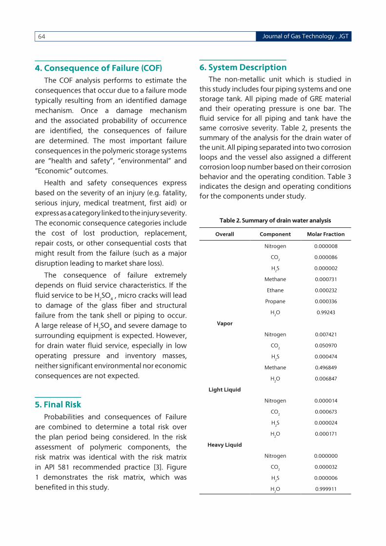
64 Journal of Gas Technology . JGT
ـــــــــــــــــــــــــــــــــــــــــــــــــــــــــــــــــــــــ4. Consequence of Failure (COF)
The COF analysis performs to estimate the
consequences that occur due to a failure mode
typically resulting from an identified damage
mechanism. Once a damage mechanism
and the associated probability of occurrence
are identified, the consequences of failure
are determined. The most important failure
consequences in the polymeric storage systems
are “health and safety”, “environmental” and
“Economic” outcomes.
Health and safety consequences express
based on the severity of an injury (e.g. fatality,
serious injury, medical treatment, first aid) or
express as a category linked to the injury severity.
The economic consequence categories include
the cost of lost production, replacement,
repair costs, or other consequential costs that
might result from the failure (such as a major
disruption leading to market share loss).
The consequence of failure extremely
depends on fluid service characteristics. If the
fluid service to be H2SO
4 , micro cracks will lead
to damage of the glass fiber and structural
failure from the tank shell or piping to occur.
A large release of H2SO
4 and severe damage to
surrounding equipment is expected. However,
for drain water fluid service, especially in low
operating pressure and inventory masses,
neither significant environmental nor economic
consequences are not expected.
ــــــــــــــــــــــــــ5. Final Risk
Probabilities and consequences of Failure
are combined to determine a total risk over
the plan period being considered. In the risk
assessment of polymeric components, the
risk matrix was identical with the risk matrix
in API 581 recommended practice [3]. Figure
1 demonstrates the risk matrix, which was
benefited in this study.
ـــــــــــــــــــــــــــــــــــــــــــــــــ6. System Description
The non-metallic unit which is studied in this study includes four piping systems and one storage tank. All piping made of GRE material and their operating pressure is one bar. The fluid service for all piping and tank have the same corrosive severity. Table 2, presents the summary of the analysis for the drain water of the unit. All piping separated into two corrosion loops and the vessel also assigned a different corrosion loop number based on their corrosion behavior and the operating condition. Table 3 indicates the design and operating conditions for the components under study.
Table 2. Summary of drain water analysis
Overall Component Molar Fraction
Nitrogen 0.000008
CO2
0.000086
H2S 0.000002
Methane 0.000731
Ethane 0.000232
Propane 0.000336
H2O 0.99243
Vapor
Nitrogen 0.007421
CO2
0.050970
H2S 0.000474
Methane 0.496849
H2O 0.006847
Light Liquid
Nitrogen 0.000014
CO2
0.000673
H2S 0.000024
H2O 0.000171
Heavy Liquid
Nitrogen 0.000000
CO2
0.000032
H2S 0.000006
H2O 0.999911

65Volume 6 / Issue 1 / February 2020
Table 3. Polymeric components’ pre-assessment data
Corrosion Loop No. 1- Type 2-System Description3-Equipment Buried
(Yes/No) 4-Size External Diam-
eter (Inches)
D-GRE-01 Pipe DRAINS (GENERAL) YES 3
D-GRE-01 Pipe DRAINS (GENERAL) YES 4
W-GRE-02 Pipe WASH WATER YES 3
D-GRE-01 Pipe DRAINS (GENERAL) YES 4
DW-CS-03 Vessel DISTILLED WATER No 65
Table 3. Polymeric components’ pre-assessment data (Cont’d)
Corrosion Loop No.
5-Design Pres-sure (Bar)
6-Design Temperature
(Degree C)
7-Primary Fluid Phase
8-H2SO4 Exists 9-HCl Exist10- FLUID DEN-
SITY KG/ M3
D-GRE-01 7 85 Liquid No No 1000
D-GRE-01 7 85 Liquid No No 306-789
W-GRE-02 17.8 65 Liquid NO NO 1000
D-GRE-01 7 85 Liquid NO NO 306-789
DW-CS-03 1 85 Liquid NO NO 995.6
ــــــــــــــــــــــــــــــــــــــــــــــــــــــــ7. Results and Discusions
Qualitative RBI analysis is performed for the components listed in Table 3. In the calculation of the POF, the chance of occurrence of each type of damage mechanism mentioned in section 2 are considered and the weighted sum of the POF for each damage mechanism result the final POF for each component. As the fluid service is non-flammable and its toxic effect is low, the environmental side effects of the fluid release play a key role in the determination of the COF
of the components. Then, the fluid inventory and fluid composition are the main parameters in the qualitative evaluation of the COFs for components. The results of the evaluation for all three corrosion loops are presented in Table 4. As it is obvious from Table 4, the consequences for corrosion loop one (D-GRE-01) is the highest among all, as its inventory volume is the highest. Furthermore, the proposed inspection plan for these types of components are offered for each loop in Table 4.
Table 4. Overall risk and inspection plan of the polymeric components
Corrosion Loop No.
1- Mate-rial
2- POF Category
(1-5)
3- COF Category
(1-5 or A-E)
4- Overall Risk
5- Integrity Management Plan (Inspection Interval and plan)
D-GRE-01 GRE 2 C Medium Visual Inspection including depth gages, penetrants. Not > 3 yearsVisual Inspection including depth gages, penetrants. Not > 5 yearsInternal Visual Inspection focusing on Nozzle, shell, bottom transition regions and other areas of stress concentration, inspect for areas of high fluid velocities for the accelerated attack, Assess crack penetration into structural layer. Repair/patch areas of attack and install wear plates as appreciate. Not > 5 years
W-GRE-02 GRE 2 B Low
DW-CS-03 GRP 1 B Low

66 Journal of Gas Technology . JGT
Figure 1. Risk Matrix which is used in this study
ـــــــــــــــــــــــــــــــ8. Conclusion
In this paper, the risk based inspection of the
non-metallic components are described with an example of a small unit. Damage mechanisms for this type of components are listed and their probability of failure are discussed. According to the standard procedures, as the fluid service is drain or wash water, the environmental effect of the failure is much important than safety and cost criteria. Hence, the inventory volume is the much important factor in determination of the consequence of failure of the component. Based on obtained results the inspection plan for the investigated corrosion loops are proposed.
ــــــــــــــــــــــــــــــ7. References
1. Shishesaz, M.R., Bajestani, M.N., Hashemi, S.J. and Shekari, E., 2013. Comparison of API 510 pressure vessels inspection planning with API 581 risk-based inspection planning approaches. International Journal of Pressure Vessels and Piping, 111, pp. 202-208.
2. Choi, S.C., Lee, J.H., Lee, C.H., Song, K.H., Chang, Y.S. and Choi, J.B., 2007. Risk Based Approach of In-service Inspection and Maintenance for Petrochemical Industries. In Key Engineering Materials (Vol. 353, pp. 2623-2627). Tran. Tech. Publications.
3. API 581, 2019. American Petroleum Institute. Risk-based inspection technology.
Washington, D.C.: API Publishing Services.
4. API 580, 2016. American Petroleum Institute. Risk-based inspection technology. Washington, D.C.: API Publishing Services.
5. Kamsu-Foguem, B., 2016. Information structuring and risk-based inspection for the marine oil pipelines. Applied Ocean Research, 56, pp.132-142.
6. Cimellaro, G.P., Villa, O. and Bruneau, M., 2014. Resilience-based design of natural gas distribution networks. Journal of Infrastructure systems, 21(1), p.05014005.
7. Chant, E. and Sims, J.R., 2010, January. Risk-based inspection for polymers. In CORROSION 2010. NACE International.
8. SPC/Tech/Gen/35 2008. Integrity of Atmospheric Storage Tanks, HSE.
9. Zhang, B.Y., Li, H.H. and Wang, W., 2015. Numerical study of dynamic response and failure analysis of spherical storage tanks under external blast loading. Journal of Loss Prevention in the Process Industries, 34, pp. 209-217.
10. Shuai, J., Han, K. and Xu, X., 2012. Risk-based inspection for large-scale crude oil tanks. Journal of Loss Prevention in the Process Industries, 25(1), pp.166-175.
11. [11] Trebuňa, F., Šimčák, F. and Bocko, J., 2009. Failure analysis of storage tank. Engineering Failure Analysis, 16(1), pp. 26-38.
12. Radhakrishnan, S.M., Dyer, B., Kashtalyan, M., Akisanya, A.R., Guz, I. and Wilkinson, C., 2014. Analysis of bolted flanged panel joint for GRP sectional tanks. Applied Composite Materials, 21(1), pp. 247-261.
13. Mercy, D. and Girirajkumar, S.M., 2017, July. An algorithmic approach based pso-pid tuning of a real time conical tank process used in waste water treatment. In 2017 International Conference on Computing Methodologies and Communication (ICCMC) (pp. 871-876).

67Volume 6 / Issue 1 / February 2020
IEEE.
14. Asghari, F.B., Jafari, J., Yousefi, M., Mohammadi, A.A. and Dehghanzadeh, R., 2018. Evaluation of water corrosion, scaling extent and heterotrophic plate count bacteria in asbestos and polyethylene pipes in drinking water distribution system. Human and Ecological Risk Assessment: An International Journal, 24(4), pp.1138-1149.
15. Foulon, A., Laksimi, A., Lemaître, C. and Favergeon, J., 2014. Use of acoustic emission technique for in service evaluation of the mechanical integrity of equipment GRP (Glass reinforced plastic). In 16th European Conference on Composite Materials.
16. Association, N.O.A.G., Norwegian Oil and Gas Association Recommended Guidelines for NDT of GRP pipe systems.
17. Norway, S., Fabrication and installation of GRP piping systems, in Norsok Standard M-622.2005.

68 Journal of Gas Technology . JGT
شبیه سازی و تحلیل ترمودینامیکی فرآیند انبساطی نیتروژن چرخه بسته برای مایع-سازی گاز طبیعی در مقیاس کوچک
امیرحسین•یزدانی•نیا۱،•علی•وطنی۱*•،•مرضیه•زارع۲،•مژگان•عباسی3••• انستیتو•گاز•طبیعی•مایع•)ILNG(،•گروه•مهندسی•شیمی،•دانشکده•فنی،•دانشگاه•تهران،•تهران،•ایران.۱.
• شرکت•ملی•گاز•ایران،•تهران،•ایران.۲.
• انستیتو•مهندسی•نفت،•گروه•مهندسی•شیمی،•دانشکده•فنی،•دانشگاه•تهران،•تهران،•ایران.3.
) [email protected] •:ایمیل•نویسنده•مسئول(
ـــــــــــــــــــــــ
چکیــــده
در این پژوهش، یک چرخه انبساطی نیتروژن بسته )Niche( با استفاده از نرم افزار Aspen HYSYS V8.4 شبیه سازی گردیده است. به منظور ارزیابی فرآیند مذکور از تحلیل های انرژی و اکسرژی استفاده شده است. نتایج حاصل از تحلیل انرژی نشان داد که میزان توان ویژه مصرفی این فرآیند برابر kWh/kg LNG ۰/۶۸ می باشد. نتایج حاصل از تحلیل اکسرژی نیز نشان داد که راندمان اکسرژی فرآیند Niche LNG برابر ٪۳۵/۵۱ است. نتیجه حاصل از این دو تحلیل تعامل بین توان ویژه مصرفی و راندمان اکسرژی بود. علاوه بر این، بالاترین
مقدار راندمان و اتلاف اکسرژی، به ترتیب متعلق به کمپرسور C3 و توربین گازی E1 است. همچنین می توان گفت این فرآیند برای واحدهای مقیاس کوچک LNG می تواند گزینه مناسبی است.
.)LNG( واژگان کلیدی: چرخه انبساطی نیتروژن بسته ، تحلیل اکسرژی، توان ویژه مصرفی، گاز طبیعی مایع

69Volume 6 / Issue 1 / February 2020
شبیه سازی تولید توان الکتریکی با استفاده از توربین های انبساطی در ایستگاه Aspen Plus های تقلیل فشار گاز طبیعی با استفاده از نرم افزار
بیژن•حجازی۱*،•فتح•ا...•فرهادی۲••• استادیار•گروه•مهندسی•شیمی،•دانشکده•مهندسی،•دانشگاه•فردوسی•مشهد،•مشهد،•ایران.۱.
• استاد•دانشکده•مهندسی•شیمی•و•نفت،•دانشگاه•صنعتی•شریف،•تهران،•ایران.•۲.
)[email protected] •:ایمیل•نویسنده•مسئول(
ـــــــــــــــــــــــ
چکیــــده
این مقاله امکان سنجی اقتصادی تولید برق پراکنده از بازیافت اکسرژی جریان گاز طبیعی تحت فشار از طریق نصب توربین انبساطی به موازات شیر فشار شکن در ایستگاه تقلیل فشار شهری را مورد مطالعه قرار می دهد. احتیاجات پیش گرمایشی مورد نیاز برای جلوگیری از تشکیل هیدرات بر اثر افت فشار توسط احتراق کسر کوچکی از جریان گاز طبیعی خروجی تامین می گردد. به عنوان مطالعه موردی، شبیه سازی ایستگاه دروازه شهری شماره 2 شهر تهران بیانگر اتلاف اکسرژی بیش از ۳۶/۵ میلیون کیلووات ساعت در سال توسط شیرهای فشار شکن موجود است. آنالیزهای ترمودینامیکی و اقتصادی، شرایط عملیاتی بهینه برای تولید برق توسط توربین انبساطی را بدست می دهند. بهینه سازی دمای پیش گرمایش منجر به بیش از ۰۶ درصد بازیافت اکسرژی، هزینه برق تولیدی کمتر از ۰.۰۴ دلار بر کیلووات ساعت و زمان بازگشت سرمایه حدود ۴ سال می گردد. از نتایج شبیه سازی ها می توان برای طراحی سیستم کنترل خودکار دمای پیش گرمایش به منظور
بهینه سازی بازیافت اکسرژی توسط توربین انبساطی تحت شرایط عملیاتی متغیر ایستگاه تقلیل فشار گاز استفاده نمود.
واژگان کلیدی: گاز طبیعی، ایستگاه تقلیل فشار، توربین انبساطی، شبیه سازی فرایند.

70 Journal of Gas Technology . JGT
شبیه سازی جداکننده سه فازصنعتی دارای بوت با استفاده از دینامیک سیالات محاسباتی
زهره•خلیفات۱،•مرتضی•زیودار۲*،•رهبر•رحیمی3••• دانشجوی•دکتری•مهندسی•شیمی،•گروه•مهندسی•شیمی،•دانشگاه•سیستان•و•بلوچستان،•زاهدان،•ایران.۱.
• استاد•گروه•مهندسی•شیمی،•دانشگاه•سیستان•و•بلوچستان،•زاهدان،•ایران.۲.
• استاد•گروه•مهندسی•شیمی،•دانشگاه•سیستان•و•بلوچستان،•زاهدان،•ایران.3.
) [email protected] •:ایمیل•نویسنده•مسئول(
ـــــــــــــــــــــــ
چکیــــده
جداکننده های سه فازی برای جدایش فازهای غیر قابل امتزاج در صنایع نفتی مورد استفاده قرار می گیرند. شبیه سازی این جداکننده های صنعتی با استفاده از دینامیک سیالات محاسباتی در مراجع بسیار محدود بوده و اکثر کارها ی انجام شده مربوط به شبیه سازی با استفاده از دیدگاه اولر-اولر یا اولر-لاگرانژ با تطابق ضعیف بین نتایج مربوط به شبیه سازی و داده های صنعتی بوده است . در این کار یک مدل که ترکیبی از دو مدل حجم سیال)FOV(و مدل فاز ناپیوسته )MPD( که ترکیب دو دیدگاه اولر-اولر و اولر-لاگرانژ بوده، برای شبیه سازی یک جداکننده سه فاز صنعتی دارای بوت توسعه داده شده است. لازم به ذکر است که با وجود کاربرد گسترده جداکننده های دارای بوت در صنایع نفتی، تا کنون هیچ پژوهشی روی این نوع از جداساز ها انجام نشده است .به منظور توسعه این مدل ترکیبی در این کار، اثر زیر مدل های مختلف شامل نیروی جرم مجازی، شکست قطرات و مدل گام تصادفی )WRD( که در اکثر شبیه سازی ها از آن صرف نظر شده، مورد بررسی قرار گرفته است. میزان جرم قطرات در گاز خروجی از داده های مربوط به جداکننده موجود در شرکت پتروشیمی برزویه واقع در جنوب ایران به عنوان معیاری برای ارزیابی مدل مورد نظر، مورد استفاده قرار گرفته است. نتایج نشان داد که مدل ترکیبی مورد نظر با در نظر گرفتن هر سه زیر مدل و تاثیر بالای زیرمدل WRD یک مدل موفق در تخمین بازده جداکننده بوده است، به طوری که با استفاده از زیر مدل ها خطای نتایج شبیه سازی از۴۰/۸۱ ٪ به ۱2/9٪ کاهش پیدا کرده است. در این کار همچنین با استفاده از مدل اعتبار سنجی شده به بررسی اثر اندازه قطرات و دبی ورودی روی عملکرد جدا کننده پرداخته شده است. نتایج نشان دادند که کاهش اندازه قطرات) به اندازه ۰2٪( و افزایش دبی)۶۴7۵kg/hr -۵۸۰۰( باعث کاهش راندمان جداساز شده است به طوری که میزان جرم قطرات مایع در گاز خروجی به
ترتیب به اندازه 29٪ و ۳۸٪ افزایش یافته است.
واژگان کلیدی: دینامیک سیالات محاسباتی، جریان چند فازی، شبیه سازی، جداکننده سه فاز دارای بوت، مدل گام تصادفی.

71Volume 6 / Issue 1 / February 2020
بهینه سازی عملکرد جداسازی غشای بهبود یافته لایه نازک کامپوزیتیPebax MH1657 با استفاده از روش طراحی آزمایش
طیبه•خسروی*••• گروه•مهندسی•ایمنی،•دانشگاه•علم•و•فرهنگ،•صندوق•پستی•۱7854۱3۱،•تهران،•ایران.۱.
)[email protected] •:ایمیل•نویسنده•مسئول(
ـــــــــــــــــــــــ
چکیــــده
در این پژوهش، روش طراحی آزمایش CCD به منظور بهینه سازی و تجزیه و تحلیل اثر افزودن پلیمر)%PEG-ran-PPG )10-50 wt بعنوان CO غشای
2/CH
4CO و گزینش پذیری
2پلیمر آلیاژکار و ذرات CuBTC (0–20 wt%) که یک نوع MOF بوده بعنوان نانوذرات بر روی تراوایی گاز
لایه نازک کامپوزیتی Pebax MH 1657/polysulfone مورد استفاده قرار گرفته است. در حقیقت خصوصیات مثبت آلیاژکاری و غشاهای PEG-ran-PPG ماتریس آمیخته بصورت همزمان در این پژوهش مورد استفاده قرار گرفته است. بر اساس ضرایب مدل برازش، درصد وزنیCO داشته است. نتایج
2/CH
4CO داشته درحالیکه درصد وزنی CuBTC بیشترین تاثیر را بر روی گزینش پذیری
2اثر زیادی بر روی تراوایی
CO تقریبا ۶2۰ درصد 2آزمایشگاهی و آماری نشان دادند که تحت شرایط بهینه(%PEG-ran-PPG: 32.76 wt% and CuBTC: 20 wt)، تراوایی
CO حدود ۴۳ درصد در مقایسه با غشای Pebax افزایش پیدا کرد.2/CH
4و گزینش پذیری
.CCD غشای کامپپوزیتی، روش طراحی آزمایش ،Pebax ،دواژگان کلیدی: جداسازی دی اکسید کربن

72 Journal of Gas Technology . JGT
مخازن استراتژیک گاز در لایه های نمک و اثرات خزش و سربار بر کاهش حجم
علیرضا•سلطانی۱،•حسن•میرزابزرگی۲*•••۱و۲.••••دانشکده•مهندسی•عمران،•دانشگاه•صنعتی•خواجه•نصیرالدین•طوسی،•تهران،•ایران.
)[email protected] •:ایمیل•نویسنده•مسئول(
ـــــــــــــــــــــــ
چکیــــده
تقاضا برای سوخت های فسیلی مانند گاز طبیعی، نفت و دیگر محصولات هیدروکربنی در دهه های اخیر افزایش یافته است. پاسخ گویی به این تقاضا در دوره اوج مصرف، اهمیت ذخیره سازی منابع انرژی را در دوره تولید نشان می دهد. در ارتباط با این موضوع، ذخیره کردن گاز در حفره های نمکی روش مناسبی است. برای توصیف رفتار مکانیکی یک سنگ نمک عادی بر اثر پدیده خزش، مدل ساختاری خزش تغییرشکل دارای چند مکانیزم )MD( در نرم افزار اجزا محدود ANSYS با استفاده از یک روتین Fortran گنجانده شد. جهت بررسی اثر خزش بر پاسخ سازه ای و کاهش حجم یک حفره نمکی، تحلیل خزش ضمنی تحت بارهای چرخه ای انجام شد. نتایج نشان می دهد که اعمال بارهای فشاری سربار به کاهش حجم کمتری در حفره نمکی می انجامد، در حالی که قراردادن خود لایه سربار بر لایه نمک بجای فشار
سربار، کاهش حجم کمتری را در پی دارد. نهایتا، با استفاده از المان تماس بین لایه سربار و لایه نمک کاهش حجم، کمتر هم خواهد بود.
دواژگان کلیدی: حفره نمکی، مدل خزش MD، سنگ نمک، خزش ضمنی، کاهش حجم، بارگذاری چرخه ای.

73Volume 6 / Issue 1 / February 2020
بازرسی بر مبنای ریسک اجزای کامپوزیتی در صنایع نفت و گاز
میثم•نجفی•ارشادی۱،•مهدی•اسکندرزاده۲*،•علی•کلاکی۲••• گروه•مهندسی•مکانیک،•دانشکده•فنی•و•مهندسی،•دانشگاه•محقق•اردبیلی،•اردبیل،•ایران.۱.
• دپارتمان•حفاظت•فنی•و•خوردگی،•شرکت•نفت•مناطق•مرکزی•ایران،•تهران،•ایران.۲.
) [email protected] •:ایمیل•نویسنده•مسئول(
ـــــــــــــــــــــــ
چکیــــده
هدف از فعالیت های بازرسی فنی اطمینان از کارکرد اجزاء در شرایط ایمن است. در حال حاضر، رویکرد اصلی در بخش بازرسی فنی حرکت به سمت راهبردهای بازرسی با صرفه اقتصادی و نیز قابلیت اطمینان بالا است. بازرسی بر مبنای ریسک )RBI( فرایند ایجاد برنامه بازرسی بر اساس دانشی است که از ریسک خرابی تجهیز بدست می آید. بطور کلی روش RBI مبتنی بر ترکیب دو عنصر احتمال خرابی در نتیجه آسیب، کاهش کارایی و یا تخریب تجهیز و پیامدهای چنین خرابی ها است. RBI به افزایش ایمنی واحد و کارخانه کمک کرده، هزینه ها را کاهش و حفاظت از محیط زیست را بهبود می بخشد. هم اکنون روش RBI به عنوان بخش مرکزی بسیاری از استراتژی های بازرسی در صنعت نفت و گاز ارزیابی می شود. با این حال، استفاده از RBI در اجزای غیر فلزی کمتر مورد مطالعه قرار گرفته شده است. لذا در این مقاله، به ارزیابی ریسک اجزای GRE/GRP پرداخته شده است. اجزای کامپوزیتی به طور گسترده در سیستم های انتقال و ذخیره آب )شامل پساب ، فاضلاب و آب شستشو( استفاده می شود. در این پژوهش، مکانیزم های مختلف خرابی در اجزای کامپوزیتی مورد بحث قرار گرفته شد. نتایج ارزیابی TEM نشان داد که اجزای کامپوزیتی این مطالعه بایستی در سال دوم پس از شروع بهره برداری مورد بازرسی قرار گیرند. از آنجا که بر اساس ارزیابی صورت پذیرفته متوسط ریسک کلی اجزا کم است، بنابراین بازرسی چشمی برای دوره های سه الی پنج ساله
برای لوله ها و مخازن غیر فلزی این کار پیشنهاد شده است.
واژگان کلیدی: بازرسی فنی، مخازن GRE/GRP، بازرسی بر مبنای ریسک، خوردگی.

1 Simulation and Thermodynamic Analysis of a Closed Cycle Nitrogen Expansion Process for Liquefaction of Natural Gas in Mini-scale
Amirhossein Yazdaninia, Ali Vatani, Marzieh Zare, Mojgan Abbasi
2 Aspen Plus Simulation of Power Generation Using Turboexpanders in Natural Gas Pressure Reduction Stations
Bijan Hejazi, Fatollah Farhadi
3 Simulation of an Industrial Three Phase Boot Separator Using Computational Fluid Dynamics
Zohreh Khalifat, Mortaza Zivdar, Rahbar Rahimi
4 Optimizing CO2/CH4 Separation Performance of Modified Thin Film Composite Pebax MH 1657 Membrane Using a Statistical Experimental Design Technique
Tayebeh Khosravi
5 Strategic Storages of Gas in Salt Layers and Creep and Overburden Effects on Volume Loss
Alireza Soltani, Hassan Mirzabozorg
6 Risk Based Inspection of Composite Components in Oil and Gas Industry
Meysam Najafi Ershadi, Mehdi Eskandarzade, Ali Kalaki