journal of control science and engineering
TRANSCRIPT

Model Predictive Control
Guest Editors: Baocang Ding, Marcin T. Cychowski, Yugeng Xi, Wenjian Cai, and Biao Huang
Journal of Control Science and Engineering

Model Predictive Control

Journal of Control Science and Engineering
Model Predictive Control
Guest Editors: Baocang Ding, Marcin T. Cychowski,Yugeng Xi, Wenjian Cai, and Biao Huang

Copyright © 2012 Hindawi Publishing Corporation. All rights reserved.
This is a special issue published in “Journal of Control Science and Engineering.” All articles are open access articles distributed underthe Creative Commons Attribution License, which permits unrestricted use, distribution, and reproduction in any medium, providedthe original work is properly cited.

Editorial Board
Zhiyong Chen, AustraliaEdwin K. P. Chong, USARicardo Dunia, USANicola Elia, USAPeilin Fu, USABijoy K. Ghosh, USAF. Gordillo, SpainShinji Hara, Japan
Seul Jung, Republic of KoreaVladimir Kharitonov, RussiaDerong Liu, ChinaTomas McKelvey, SwedenSilviu-Iulian Niculescu, FranceYoshito Ohta, JapanYang Shi, CanadaS. Skogestad, Norway
Zoltan Szabo, HungaryOnur Toker, TurkeyXiaofan Wang, ChinaJianliang Wang, SingaporeWen Yu, MexicoL. Z. Yu, ChinaMohamed A. Zribi, Kuwait
Contents
Model Predictive Control, Baocang Ding, Marcin T. Cychowski, Yugeng Xi, Wenjian Cai, and Biao HuangVolume 2012, Article ID 240898, 2 pages
Distributed Model Predictive Control of the Multi-Agent Systems with Improving Control Performance,Wei Shanbi, Chai Yi, and Li PenghuaVolume 2012, Article ID 313716, 8 pages
Model Predictive Control of Uncertain Constrained Linear System Based on Mixed H2/H∞ ControlApproach, Patience E. OrukpeVolume 2012, Article ID 402948, 12 pages
Experimental Application of Predictive Controllers, C. H. F. Silva, H. M. Henrique,and L. C. Oliveira-LopesVolume 2012, Article ID 159072, 18 pages
Robust Model Predictive Control Using Linear Matrix Inequalities for the Treatment of AsymmetricOutput Constraints, Mariana Santos Matos Cavalca, Roberto Kawakami Harrop Galvao,and Takashi YoneyamaVolume 2012, Article ID 485784, 7 pages
Efficient Model Predictive Algorithms for Tracking of Periodic Signals, Yun-Chung Chu andMichael Z. Q. ChenVolume 2012, Article ID 729748, 13 pages
Pole Placement-Based NMPC of Hammerstein Systems and Its Application to Grade Transition Controlof Polypropylene, He De-Feng and Yu LiVolume 2012, Article ID 630645, 6 pages

Hindawi Publishing CorporationJournal of Control Science and EngineeringVolume 2012, Article ID 240898, 2 pagesdoi:10.1155/2012/240898
Editorial
Model Predictive Control
Baocang Ding,1 Marcin T. Cychowski,2 Yugeng Xi,3 Wenjian Cai,4 and Biao Huang5
1 Ministry of Education Key Lab For Intelligent Networks and Network Security (MOE KLINNS Lab),Department of Automation, School of Electronic and Information Engineering, Xi’an Jiaotong University, Xi’an 710049, China
2 NIMBUS Centre for Embedded Systems Research, Cork Institute of Technology, Rossa Avenue, Cork, Ireland3 Department of Automation, Shanghai Jiaotong University, Shanghai 200240, China4 School of Electronic and Electrical Engineering, Nanyang Technological University, BLK S2, Singapore 6397985 Department of Chemical and Materials Engineering, University of Alberta, Edmonton, AB, Canada T6G 2G6
Correspondence should be addressed to Baocang Ding, [email protected]
Received 9 February 2012; Accepted 9 February 2012
Copyright © 2012 Baocang Ding et al. This is an open access article distributed under the Creative Commons Attribution License,which permits unrestricted use, distribution, and reproduction in any medium, provided the original work is properly cited.
Model predictive control (MPC) has been a leading technol-ogy in the field of advanced process control for over 30 years.At each sampling time, MPC optimizes a performance costsatisfying the physical constraints, which is initialized by thereal measurements, to obtain a sequence of control movesor control laws. However, MPC only implements the controlmove corresponding to the current sampling time. At thenext sampling time, the same optimization problem is solvedwith renewed initialization. In order to obtain offset-freecontrol, the system model is augmented with a disturbancemodel to capture the effect of model-pant mismatch. Thestate and disturbance estimates are utilized to initialize theoptimization problem. A steady-state target calculation unitis constructed to compromise between what is desired byreal-time optimization (RTO) and what is feasible for thedynamic control move optimization. As a result, MPC ex-hibits innumerous research issues from both theoretical andpractical aspects. Nowadays, there is big gap between thetheoretical investigations and industrial applications. Themain focus of this special issue is on the new research ideasand results for MPC.
A total number of 14 papers were submitted for this spe-cial issue. Out of the submitted papers, 6 contributions havebeen included in this special issue. The 6 papers consider 6rather different, yet interesting topics.
A synthesis approach of MPC is the one with guaranteedstability. The technique of linear matrix inequality (LMI) isoften used in the synthesis approach to address the satis-faction of physical constraints. However, the existing LMIformulations are for symmetric constraints. M. S. M. Cavalca
et al. treat asymmetric output constraints in integrating SISOsystems based on pseudoreferences.
Usually, the steady-state target calculation, followed withthe dynamic move calculation, is implemented in each sam-pling time. This is not practical for fast-sampling systems.Y. C. Chu and M. Z. Q. Chen propose a method to tacklethis issue. In their method, the steady-state target calculationworks in parallel to, with a period longer than and a scale ofoptimization larger than, the dynamic move calculation. It isshown that their method is particularly suitable for trackingthe periodic references.
The nonlinear system represented by a Hammersteinmodel has always been a good platform for control algorithmresearch. D. F. He and L. Yu revisit this topic by invokingthe pole-placement method on the linear subsystem. Theypropose the algorithm which consists of three online steps,instead of the two-step MPC. They also propose to usetheir algorithm in the grade transition control of industrialpolypropylene plants, via a simulation study.
Usually, MPC has its own paradigm for robust control.However, combing MPC with H2/H∞ control could be agood topic for improving the robustness of MPC. P. E.Orukpe applies the mixed H2/H∞ method in MPC where thesystem uncertainties are modeled by perturbations in a linearfractional transform (LFT) representation and unknownbounded disturbances.
Interests in the cooperative control of multi-agent sys-tems have been growing significantly over the last years. MPChas the ability to redefine cost functions and constraints asneeded to reflect changes in the environment, which makes

2 Journal of Control Science and Engineering
it a nice choice for multiagent systems. S. B. Wei et al. givea method for distributed MPC which punishes, in the costfunction, the deviation between what an agent optimizes andwhat other related agents think of it. The deviation weightmatrix at the end of the control horizon is specially discussedfor improving the control performance.
Besides, C. H. F. Silva et al. report some experimentalstudies for two classical algorithms: infinite horizon MPCand MPC with reference system. The pilot plant is for leveland pH control, which has physical constraints and nonlin-ear dynamics.
We hope the readers of Journal of Control Science andEngineering will find the special issue interesting and stim-ulating, and expect that the included papers contribute tofurther advance the area of MPC.
Acknowledgments
We would like to thank all the authors who have submittedpapers to the special issue and the reviewers involved in therefereeing of the submissions.
Baocang DingMarcin T. Cychowski
Yugeng XiWenjian CaiBiao Huang
Hindawi Publishing CorporationJournal of Control Science and EngineeringVolume 2012, Article ID 313716, 8 pagesdoi:10.1155/2012/313716
Research Article
Distributed Model Predictive Control of the Multi-AgentSystems with Improving Control Performance
Wei Shanbi, Chai Yi, and Li Penghua
College of Automation, Chongqing University, Chongqing 400044, China
Correspondence should be addressed to Wei Shanbi, [email protected]
Received 8 October 2011; Revised 22 December 2011; Accepted 19 January 2012
Academic Editor: Yugeng Xi
Copyright © 2012 Wei Shanbi et al. This is an open access article distributed under the Creative Commons Attribution License,which permits unrestricted use, distribution, and reproduction in any medium, provided the original work is properly cited.
This paper addresses a distributed model predictive control (DMPC) scheme for multiagent systems with improving controlperformance. In order to penalize the deviation of the computed state trajectory from the assumed state trajectory, the deviationpunishment is involved in the local cost function of each agent. The closed-loop stability is guaranteed with a large weightfor deviation punishment. However, this large weight leads to much loss of control performance. Hence, the time-varyingcompatibility constraints of each agent are designed to balance the closed-loop stability and the control performance, so thatthe closed-loop stability is achieved with a small weight for the deviation punishment. A numerical example is given to illustratethe effectiveness of the proposed scheme.
1. Introduction
Interests in the cooperative control of multiagent systemshave been growing significantly over the last years. The mainmotivation is the wide range of military and civilian appli-cations, including formation flight of UAV and automatedtraffic systems. Compared with the traditional approach,model predictive control (MPC), or receding horizon control(RHC) has the ability to redefine cost functions and con-straints as needed to reflect changes in the system and/orthe environment. Therefore, MPC is extensively applied tothe cooperative control of multiagent systems, which makesthe agents operate close to the constraint boundaries andobtain better performance than traditional approaches [1–3]. Moreover, due to the computational advantages and theconvenience of communication, distributed MPC (DMPC)is recognized as a nature technique to address trajectoryoptimization problems for multiagent systems.
One of the challenges for distributed control is to en-sure that local control actions keep consistent with theactions of others agents [4, 5]. For the coupled systems,the local optimization problem is solved based on thestates of its neighbors’ at sample time instant using Nash-optimization technique in [6]. As the local controllers lack
of communication and cooperation, the local control actionscannot keep consistent [7, 8]. require each local controllerexchange information with all other local controllers toimprove optimality and consistency based on sufficientcommunication. For the decoupled systems [9], exploitsthe estimation of the prediction state trajectories of theneighbors’ [10]; treats the prediction state trajectories of theneighbor agents as bounded disturbance where a min-maxoptimal problem is solved for each agent with respect to theworst-case disturbance. In [11, 12], the optimal variables ofthe local optimization problem contain the control actionof its own and its neighbors’ which are coupled in collisionavoidance constraints and cost function. Obviously, thedeviation between the actions of what the agent is actuallydoing and of what its neighbor estimates for it affectsthe control performance. Sometimes the consistency andcollision avoidance cannot be achieved, and the feasibilityand stability of this scheme cannot be guaranteed [13].proposes a distributed MPC with a fixed compatibilityconstraint to restrict the deviation. When the bound of thisconstraint is sufficiently small, the closed-loop system stateenter a neighborhood of the objective state [14, 15] give animprovement over [13] by adding deviation punishment termto penalize the deviation of the computed state trajectory

2 Journal of Control Science and Engineering
from the assumed state trajectory. Closed-loop exponentialstability follows if the weight on the deviation function termis large enough. But the large weight leads to the loss of thecontrol performance.
A contribution in this paper is to propose an idea toreduce the adverse effect of the deviation punishment onthe control performance. At each sample time, the valueof compatibility constraint is set as the maximum valueof the deviation of the previous sample time. We give thestability condition to guarantee the exponential stability ofthe global closed-loop system with a small weight on thedeviation punishment term, which is obtained by dividingthe centralize stability constraint as the manner of [16, 17].The effectiveness of the scheme is also demonstrated by anumerical example.
Notations. xik is the value of vector xi at time k · xik,t is thevalue of vector xi at a future time k + t, predicted at timek · |x| = [|x1|, |x2|, . . . , |xN |] is the absolute value for eachcomponent of x. For a vector x and positive-definite matrixQ, ‖x‖2
Q = xTQx.
2. Problem Statement
Let us consider a system which is composed of Na agents. Thedynamics of agent i [11] is
xik+1 = f i(xik,uik
), (1)
where uik ∈ Rmi , xik ∈ Rni , and f i : Rni × Rmi �→ Rni ,are the input, state, and state transition function of agent
i, respectively. uik = [ui,1k , . . . ,ui,mi
k ]T
, xik = [xi,1k , . . . , xi,nik ]T
.The sets of feasible input and state of agent i are denoted asUi ⊂ Rmi and Xi ⊂ Rni , respectively, that is,
uik ∈Ui, xik ∈Xi, k ≥ 0. (2)
At each time k, the control objective is [18] to minimize
Jk =∞∑
t = 0
[‖xk,t‖2
Q + ‖uk,t‖2R
](3)
with respect to uk,t, t ≥ 0, where x = [(x1)T, . . . , (xNa)T
]T
,
u = [(u1)T, . . . , (uNa)T
]T
; xik,t+1 = f i(xik,t,uik,t), xik,0 = xik; Q =
QT > 0, R = RT > 0. u ∈ Rm, m = ∑i mi, and x ∈ Rn,
n =∑i ni. Then,
xk+1 = f (xk,uk), (4)
where f = [ f 1, f 2, . . . , f Na]T
, f : Rn × Rm �→ Rn.(xie,u
ie) is the equilibrium point of agent i, and (xe,ue) is the
corresponding equilibrium point of all agents. X = X1 ×X2×· · ·×XNa , U =U1×U2×· · ·×UNa . The models forall agents are completely decoupled. The coupling betweenagents arises due to the fact that they operate in the sameenvironment, and that the “cooperative” objective is imposedon each agent by the cost function. Hence, there are the
coupling cost function and coupling constraints [19]. Thecoupling constraints can be transformed to coupling costfunction term directly or handled as decoupling constraintsusing the technique of [15]. In the present paper we will notconsider this issue.
The control objective for all system is to cooperativelyasymptotically stabilize all agents to an equilibrium point(xe,ue) of (4). In this paper we assumed that the (xe,ue) =(0, 0), f (xe,ue) = 0. The corresponding equilibrium pointfor each agent is (xie,u
ie) = (0, 0), f i(xie,u
ie) = 0. Assumption
f i(0, 0) = 0 is not restrictive, since if (xie,uie) /= (0, 0), one can
always shift the origin of the system to it.The resultant control law for minimization of (3) can
be implemented in a centralized way. However, the existingmethods for centralized MPC are only computationallytractable for small-scale system. Furthermore, the communi-cation cost of implementing a centralized receding horizoncontrol law may be costly. Hence, by means of decomposi-tion, Jk is divided as J ik’s such that the minimization of (3) isimplemented in distributed manner, with
J ik =∞∑
t=0
[‖zik,t‖2
Qi+ ‖uik,t‖2
Ri
], Jk =
Na∑
i=1
J ik, (5)
where zik,t = [(xik,t)T
(x−ik,t)T
]T
; x−ik,t includes the states of theneighbors. The set of neighbors’ of agent i is denoted as Ni.
x−ik = {x jk | j ∈ Ni}, x−ik ∈ Rn−i , n−i = ∑
j∈Nin j . For
each agent i, the control objective is to stabilize it to the
equilibrium point (xie,uie) · Qi = Q
Ti > 0, Ri = R
Ti > 0.
Qi is obtained by dividing Q using the technique of [19].For the agents that have decoupled dynamics, the couplingsof control moves for all system are not considered. R is adiagonal matrix and Ri is directly obtained.
Under the networked environment, the bandwidth limi-tation can restrict the amount of information exchange [17].It is thus appropriate to allow agents to exchange informationonly once in each sampling interval. We assume that theconnectivity of the interagent communication network issufficient for agents to obtain information regarding all thevariables that appear in their local problems.
In the receding horizon control manner, a finite-horizoncost function is exploited to approximate J ik. According tothe (5), the evolution of the control moves with predictivehorizon for agent i is based on the estimation of thestate trajectories x−ik,t , t ≤ N of the neighbors’, which aresubstituted by the assumed state trajectories x−ik,t, t ≤ N as[11]. In each control interval, the transmitted informationbetween agents is the assumed state trajectories. As thecooperative consistency and efficiency of distributed controlmoves is affected for the existence of the deviation of thecomputed state trajectory from the assumed state trajectory,it is appreciate to penalize it by adding the deviationpunishment term into the local cost function.
Define
uik,t = Fi(k)xik,t , ∀t ≥ N. (6)
Fi(k) is the gain of distributed state feedback controller.

Journal of Control Science and Engineering 3
Consider
J ik =N−1∑
t=0
[‖zik,t‖2
Qi+ ‖uik,t‖2
Ri+ ‖xik,t − xik,t‖2
Ti
]
+∞∑
t=N
[‖xik,t‖2
Qi+ ‖uik,t‖2
Ri
],
(7)
where
zik,t =[(
xik,t
)T(x−ik,t
)T]T
, xik,0 = xik, (8)
x−ik,t includes the assumed states of the neighbors. Qi = QTi >
0 and Ri = RTi = Ri satisfy
diag{Q1,Q2, . . . ,QNa
} ≥ Q, diag{R1,R2, . . . ,RNa
} = R.(9)
Obviously, Qi is designed to stabilize the agent i to the localequilibrium point, independently. Qi is designed to stabilizethe agent i to the local equilibrium point with neighboragents, cooperatively. Ti is the weight on the deviationpunishment term, to penalize the deviation of the computedstate trajectory from the assumed state trajectory.
At each time k, the optimization problem for distributedMPC is transformed as:
minU
ik ,Fi(k)
J ik, s.t.(1), (2), (6), (7). (10)
U∗ik = [(u∗ik,0)
T, (u∗ik,1)
T, . . . , (u∗ik,N−1)
T]
T, only when u∗ik = u∗ik,0
is implemented, and the problem (9) is solved again at timek + 1.
Remark 1. The local deviate punishment by each agenteffects the control performance, that is, incurs the loss ofoptimality.
3. Stability of Distributed MPC
The stability of distributed MPC by simply applying theprocedure as in the centralized MPC will be discussed. Thecompact and convex terminal set Ωi is defined
Ωi ={xi ∈ Rni |
(xi)TPix
i ≤ αi}
, (11)
where Pi > 0, αi > 0 are specified such that Ωi is acontrol invariant set. So using the idea of [20, 21], onesimultaneously determines a linear feedback such that Ωi is apositively invariant under this feedback.
Define the local linearization at the equilibrium point
Ai = ∂ f i
∂xi(0, 0), Bi = ∂ f i
∂ui(0, 0). (12)
and assume that (Ai,Bi) is stabilizable. When xik,N+t, t ≥ 0enters into the terminal set Ωi, the local linear feedbackcontrol law is assumed as uik,N+t = Fi(k)xik,N+t = Kix
ik,N+t.
Ki is a constant which is calculated off line as follows.
3.1. Design of the Local Control Law. The following equationfollows for achieving closed-loop stability:
∥∥∥xik,N+t+1
∥∥∥2
Pi−∥∥∥xik,N+t
∥∥∥2
Pi≤ −
∥∥∥xik,N+t
∥∥∥2
Qi
−∥∥∥uik,N+t
∥∥∥2
Ri, t ≥ 0.
(13)
Lemma 1. Suppose that there exist Qi > 0, Ri > 0, Pi > 0,which satisfy the Lyapunov-equation:
(Ai + BiKi)TPi(Ai + BiKi)− Pi = −κiPi −Qi − KT
i RiKi,(14)
for some κi > 0. Then, there exists a constant αi > 0 such thatΩi defined in (11) satisfies (13).
Remark 2. Lemma 1 is directly obtained by referring to“Lemma 1” in [21]. For MPC, the stability margin can beadjusted by turning the value of κi according to Lemma 1.With regard to DMPC, [11] adjusts the stability margin bytuning the weight in the local cost function. The controlobjective is to asymptotically stabilize the closed-loop system,so that xik,∞ = 0 and uik,∞ = 0. For t = 0, . . . ,∞, summing(13) obtains
∞∑
t=N
[∥∥∥xik,t
∥∥∥2
Qi+∥∥∥uik,t
∥∥∥2
Ri
]≤∥∥∥xik,N
∥∥∥2
Pi. (15)
Considering both (7) and (15), yields
J ik ≤ Jik =
N−1∑
t=0
[∥∥∥zik,t
∥∥∥2
Qi+∥∥∥uik,t
∥∥∥2
Ri+∥∥∥xik,t − xik,t
∥∥∥2
Ti
]
+∥∥∥xik,N
∥∥∥2
Pi,
(16)
where Jik is a finite-horizon cost function, which consists of
a finite horizon standard cost, to specify the desired controlperformance and a terminal cost, to penalize the states at theend of the finite horizon.
The terminal region Ωi for agent i is designed, so that itis invariant for nonlinear system controlled by a local linearstate feedback. The quadratic terminal cost ‖xik,N‖2
Pi boundsthe infinite horizon cost of the nonlinear system startingfrom Ωi and controlled by the local linear state feedback.
3.2. Compatibility Constraint for Stability. As in [18], wedefine two terms, ξ−i = x−∗i − x−i, ξi = x∗i − xi,
Qi =⎡⎣ Q
1i Q
12i(
Q12i
)TQ
3i
⎤⎦,
C∗x (k) =Na∑
i=1
N−1∑
t=1
{2(x∗ik,t
)TQ
12i ξ−ik,t
+2(x−ik,t
)TQ
3i ξ−ik,t +
(ξ−ik,t
)TQ
3i ξ−ik,t
},
C∗ξ (k) =Na∑
i=1
N−1∑
t=1
(ξik,t
)TTiξ
ik,t ,
(17)

4 Journal of Control Science and Engineering
Lemma 2. Suppose that (9) holds and there exits ρ(k) suchthat, for all k > 0,
0 ≤ ρ(k) ≤ 1,
− ρ(k)Na∑
i=1
{∥∥∥∥(xi(k)
)T,(x−ik)T∥∥∥∥
2
Qi
+∥∥∥u∗i(0 | k)
∥∥∥2
Ri
}
+ C∗x (k)− C∗ξ (k) ≤ 0.
(18)
Then, by solving the receding-horizon optimizationproblem
minU
i(k)Jik, s.t.(1), (2), (14), (16), uik,N = Kix
ik,N , xik,N ∈ Ωi,
(19)
and implementing u∗ik,0, the stability of the global closed-loopsystem is guaranteed, once a feasible solution at time k = 0 isfound.
Proof. Define J(k) = ∑Nai=1 J
ik. Suppose, at time k, there are
optimal solution U∗ik , i ∈ {1, . . . ,Na}, which yields
J∗
(k) =Na∑
i=1
{∥∥∥∥(xik)T
,(x−ik)T∥∥∥∥
2
Qi
+∥∥∥u∗ik,0
∥∥∥2
Ri
}
+Na∑
i=1
N−1∑
t=1
{∥∥∥∥(x∗ik,t
)T,(x−ik,t
)T∥∥∥∥
2
Qi
+∥∥∥u∗ik,t
∥∥∥2
Ri
+∥∥∥∥(x∗ik,t
)T−(xik,t
)T∥∥∥∥
2
Ti
}+
Na∑
i=1
∥∥∥x∗ik,N
∥∥∥2
Pi.
(20)
At time t + 1, according to Lemma 2, Uik+1 = {u∗ik,1, . . . ,
u∗ik,N−1,Kix∗ik,N} is feasible, which yields
J(k + 1) =Na∑
i=1
N∑
t=1
{∥∥∥∥(x∗ik,t
)T,(x−∗ik,t
)T∥∥∥∥
2
Qi
+∥∥∥u∗ik,t
∥∥∥2
Ri
}
+Na∑
i=1
∥∥∥x∗ik,N+1
∥∥∥2
Pi
=Na∑
i=1
N−1∑
t=1
{∥∥∥∥(x∗ik,t
)T,(x−∗ik,t
)T∥∥∥∥
2
Qi
+∥∥∥u∗ik,t
∥∥∥2
Ri
}
+∥∥∥x∗k,N
∥∥∥2
Q+∥∥∥u∗k,N
∥∥∥2
R+∥∥∥x∗k,N+1
∥∥∥2
P,
(21)
where P = diag{P1,P2, . . . ,PNa}. By applying (9) andLemma 2, (11) guarantees that
∥∥∥x∗k,N+1
∥∥∥2
P−∥∥∥x∗k,N
∥∥∥2
P≤ −
∥∥∥x∗k,N
∥∥∥2
Q−∥∥∥u∗k,N
∥∥∥2
R. (22)
Substituting (22) into J(k + 1) yields
J(k + 1) ≤Na∑
i=1
N−1∑
t=1
{∥∥∥∥(x∗ik,t
)T,(x−∗ik,t
)T∥∥∥∥
2
Qi
+∥∥∥u∗ik,t
∥∥∥2
Ri
}
+Na∑
i=1
∥∥∥x∗ik,N
∥∥∥2
Pi.
(23)
By applying (17)–(19),
J(k + 1)− J∗
(k)
≤ −(1− ρ(k))Na∑
i=1
{∥∥∥∥(xik)T
,(x−ik)T∥∥∥∥
2
Qi
+∥∥∥u∗ik,0
∥∥∥2
Ri
}
≤ −(1− ρ(k))‖xk‖2
Q.(24)
At time k + 1, by reoptimization, J∗
(k + 1) ≤ J(k + 1).Hence, it leads to
J∗
(k + 1)− J∗
(k) ≤ −(1− ρ(k))‖xk‖2
Q
≤ −(1− ρ(k))λmin(Q)‖x(k)‖2
Q,(25)
where λmin(Q) is the minimum eigenvalue of Q. Thisindicates that the closed-loop system is exponentially stable.
Satisfaction of (18) indicates that all xik,t should notdeviate too far from their assumed values xik,t [13]. Hence,(18) can be taken as a new version of the compatibilitycondition. This compatibility condition is derived from asingle compatibility condition that collects all the states(whether predicted or assumed) with in the switchinghorizon and is disassembled to each agent in distributedmanner, which results in local compatibility constraint foreach agent.
3.3. Synthesis Approach of Distributed MPC. In the synthesisapproach, the local optimization problem incorporates theabove compatibility condition. Since x∗k,t for all agent i iscoupled with other agents through (18), it is necessary toassign the constraint to each agent so as to satisfy (18) alongthe optimization. The continued discussion on stabilitydepends on handling of (18).
Denote ξik = [ξi,1k , . . . , ξi,nik ]T
, ξ−ik = {ξ jk | j ∈ Ni}. Attime k > 0, by solving the optimization problem, there exitsa parameter E i,l
k , l = 1, . . . ,ni, for each element of ξi,lk , l =1, . . . ,ni.
Define
E i,lk = max
t
∣∣∣ξi,lk−1,t
∣∣∣, (26)
and denote E ik = [E i,1
k , . . . , E i,nik ]
T, E−ik = {E j
k | j ∈ Ni}. Attime k + 1 > 0, set following constraint for each agent i:
∣∣∣∣(xik+1,t
)T −(xik+1,t
)T∣∣∣∣ < E i
k. (27)
From (26) and (27), it is shown that ξik+1,t < E ik and ξ−ik+1,t <
E−ik .Denote
C∗ix (k) =N−1∑
t=1
{2(x∗ik,t
)TQ
12i E−ik
+2(x−ik,t
)TQ
3i E−ik +
(E−ik
)TQ
3i
(E−ik
)T}
,
(28)

Journal of Control Science and Engineering 5
3210−1−2−3
−2 0 2 4 6 8 10 12 14
Y-l
abel
(m
)
X-label (m)
(a)
3210−1−2−3
Y-l
abel
(m
)
−2 0 2 4 6 8 10 12 14
X-label (m)
(b)
3210
−1−2−3
Y-l
abel
(m
)
−2 0 2 4 6 8 10 12 14
X-label (m)
(c)
Figure 1: Evolutions of the formation with different control schemes.
C∗iξ (k) =N−1∑
t=1
(ξik,t
)TTiξ
ik,t . (29)
Then C∗x (k) ≤∑Nai=1 C
∗ix (k), C∗ξ (k) =∑Na
i=1 C∗iξ (k).
By applying (26)–(29), it is shown that (18) is guaranteedby assigning
0 ≤ ρi(k) ≤ 1,Na∑
i=1
− ρi(k)
{∥∥∥∥(xik)T
,(x−ik)T∥∥∥∥
2
Qi
+∥∥∥u∗ik,0
∥∥∥2
Ri
}
+Na∑
i=1
C∗ix (k)−Na∑
i=1
C∗iξ (k) ≤ 0.
(30)
is dispensed to agent i:
0 ≤ ρi(k) ≤ 1,N−1∑
t=1
∥∥∥ξik,t
∥∥∥2
Ti≥ −ρi(k)
{∥∥∥∥(xik)T
,(x−ik)T∥∥∥∥
2
Qi
+∥∥∥u∗ik,0
∥∥∥2
Ri
}+ C∗ix (k).
(31)
By using (26)–(28), conservativeness is introduced. Hence,(31) is more stringent than (18).
Remark 3. By adding the deviation punishment term in thelocal cost function, the closed-loop stability follows with alarge weight. The larger weight means the more loss of theperformance [14, 19]. For a small value of Ti, we can adjustthe value of ρi(k) to obtain exponential stability. As the ρi(k)is set by optimization, this scheme has more freedom totuning parameters, to balance the closed-loop stability andcontrol performance.
Remark 4. According to (31), the maximum value andminimum value of Ti can be calculated by considering therange of each variable. We choose the middle value for Ti.Obviously, the Ti is time varying and denoted as Ti(k).
4. Control Strategy
For practical implementation, distributed MPC is formu-lated in the following algorithm.
Algorithm. Off-line stage:
(i) Set the value of the prediction horizon N .
(ii) According to (3), (5) and (9), find Qi, Ri, Qi,Ri, t =0, . . . ,N − 1, for all agents.
(iii) Set the value of the compatibility constraint for allagents Ei(0) = +∞, j ∈ Ni.
(iv) Calculate the terminal weight Pi, local linear feedbackcontrol gain Ki and the terminal set Ωi.
On-line stage: For agent i, perform the following stepsat k = 0:
(i) Take the measurement of xi0. Set Ti = 0.
(ii) Send xi0 to its neighbor j, j ∈ Ni of agent i. Receive
xj0.
(iii) Set xjt,0 = x
j0,0, j ∈ Ni, t = 0, . . . ,N − 1 and xi0,t = xi0.
(iv) Solve problem (19).
(v) Implement ui0 = u∗i0,0.
(vi) Get xit,0 and the value of compatibility constraintEi(1).

6 Journal of Control Science and Engineering
(vii) Send xi0,t and Ei(1) to its neighbor j, j ∈ Ni. Receive
xj0,t and E j(1). Calculate Ti(k).
For the agent i, perform the following steps at k > 0:
(i) Take the measurement of xik.
(ii) Solve problem (19).
(iii) Implement uik = u∗i0,k.
(iv) Get xik,t and the new value of compatibility constraintEi(k + 1).
(v) Send xik,t and Ei(k + 1) to its neighbor j, j ∈ Ni.
Receive xjk,t and E j(k + 1).
(vi) Calculate Ti(k).
5. Numerical Example
We consider the model of agent i [22] as
xik+1 =[I2 I2
0 I2
]xik +
[0.5I2
I2
]uik, (32)
which is obtained by discretizing the continuous-time model
xi =[
0 I2
0 0
]xi +
[0I2
]ui. (33)
(xik = [qi,xk , qi,yk , vi,xk , v
i,yk ]
T, qi,xk and q
i,yk are positions in
the horizontal and vertical directions, resp. vi,xk and vi,yk are
velocities in the horizontal and vertical directions, resp.) withsampling time interval of 0.5 second. There are four agents.A set of positions of the four agents constitute a formation.The initial positions of the four agents are
[q1,xo , q
1,yo
]= [0, 2],
[q2,xo , q
2,yo
]= [−2, 0], (34)
[q3,xo , q
3,yo
]= [0,−3],
[q4,xo , q
4,yo
]= [2, 0]. (35)
Linear constraints on states and input are
∣∣∣xi∣∣∣ ≤
[100 100 15 15
]T,
∣∣∣ui∣∣∣ ≤
[2 2
]T. (36)
The agent i, i = 1, 2, 3 are selected as the core agents ofthe formation. A0 is designed as A0 = {(1, 2); (1, 3); (2, 4)}.If all systems achieve the desire formation and the core agents
cooperatively cover the virtue leader, then ui,xk (k) = 0, ui,yk =
0. The global cost function is obtained as
J(k) =∞∑
t=0
[∥∥∥q1k,t − q2
k,t + c12
∥∥∥2+∥∥∥q1
k,t − q3k,t + c13
∥∥∥2
+∥∥∥q2
k,t−q4k,t+c24
∥∥∥2+
19
∥∥∥(q1k,t+q
2k,t+q
3k,t
)−qc
∥∥∥2
+∥∥∥v1
k,t
∥∥∥2+∥∥∥v2
k,t
∥∥∥2+∥∥∥v3
k,t
∥∥∥2+∥∥∥v4
k,t
∥∥∥2+∥∥uk,t
∥∥2].
(37)
They cooperatively track the virtual leader whose referenceis qc = (0.5 ∗ k, 0). The distance between agents is defined
as c12 = (−2, 1), c13 = (−2,−1), c24 = (−2, 1). Choose N1 ={2}, N2 = {1}, N3 = {1}, N4 = {2}. Then,
Q =
⎡⎢⎢⎢⎢⎢⎢⎢⎢⎢⎢⎢⎢⎢⎢⎢⎢⎣
219I2 0 −8
9I2 0 −8
9I2 0 0 0
0 I2 0 0 0 0 0 0
−89I2 0 2
19I2 0
19I2 0 −I2 0
0 0 0 I2 0 0 0 0
−89I2 0
19I2 0 1
19I2 0 0 0
0 0 0 0 0 I2 0 00 0 −I2 0 0 0 I2 00 0 0 0 0 0 0 I2
⎤⎥⎥⎥⎥⎥⎥⎥⎥⎥⎥⎥⎥⎥⎥⎥⎥⎦
, R = I8.
Q1 =
⎡⎢⎢⎢⎢⎢⎢⎢⎢⎢⎣
79I2 0 −4
9I2 0
013I2 0 0
−49I2 0 I2 0
0 0 013I2
⎤⎥⎥⎥⎥⎥⎥⎥⎥⎥⎦
,
Q2 =
⎡⎢⎢⎢⎢⎢⎢⎢⎢⎢⎣
119I2 0 −4
9I2 0
013I2 0 0
−49I2 0
49I2 0
0 0 013I2
⎤⎥⎥⎥⎥⎥⎥⎥⎥⎥⎦
,
Q3 =
⎡⎢⎢⎢⎢⎢⎢⎢⎢⎢⎣
119I2 0 −8
9I2 0
012I2 0 0
−89I2 0
89I2 0
0 0 013I2
⎤⎥⎥⎥⎥⎥⎥⎥⎥⎥⎦
,
Q4 =
⎡⎢⎢⎢⎢⎣
I2 0 −I2 00 I2 0 0−I2 0 I2 0
0 0 013I2
⎤⎥⎥⎥⎥⎦
,
(38)
and Ri = I2, i ∈ {1, 2, 3, 4}. Choose Qi = 6.85 ∗ I4 andRi = I2, i ∈ {1, 2, 3, 4}, N = 10. The terminal set is αi = 0.22.The above choice of model, cost, and constraints allow usto rewrite problem (19) as a quadratic programming withquadratic constraint. To solve the optimal control problemsnumerically, the package NPSOL 5.02 is used. From top tobottom, the first subgraph of Figure 1 is the evolution ofthe formation with central MPC; the second sub-graph ofFigure 1 is the evolution of the formation with distributedMPC with time-varying compatible constraint; the thirdsub-graph of Figure 1 is the evolution of the formation withdistributed MPC with a fixed compatibility constraint.
With the three control schemes, the formation of allagents can be achieved. The obtained Jtrue′s are 2.5779 × 106,4.8725 × 106, and 5.654 × 10⁶, respectively. Comparedwith the second sub-graph, the third sub-graph have a

Journal of Control Science and Engineering 7
1
0.8
0.6
0.4
0.2
00 5 10 15 20 25
Val
ue
Time/k
Figure 2: The value of ρi(k).
large overshoot at the time-instant k = 9 (nearby theposition (3, 0)). The distributed MPC with the time-varyingcompatible constraint has a better control process comparingto the one with fixed compatible constraint. The value ofρi(k) is shown in Figure 2. “∗” for agent 1; “O” for agent 2;“>” for agent 3; “<” for agent 4.
Remark 5. For the second simulation, the value of the fixedcompatible constraint is 0.2. For the third simulation, thevalues of the time-varying compatible constraint is calculat-ed according to the states deviation of the previous horizon.
6. Conclusions
In this paper, we have proposed an improved distributedMPC scheme for multiagent systems based on deviationpunishment. One of the features of the proposed schemeis that the cost function of each agent penalizes thedeviation between the predicted state trajectory and theassumed state trajectory, which improves the consistency andoptimal control trajectory. At each sample time, the value ofcompatibility constraint is set by the deviation of previoussample time-instant. The closed-loop stability is guaranteedwith a small value for the weight of the deviation functionterm. Furthermore, the effectiveness of the scheme has beeninvestigated by a numerical example. One of the future workswill focus on feasibility of optimization.
Acknowledgment
This work is supported by a Grant from the FundamentalResearch Funds for the Central Universities of China, no.CDJZR10170006.
References
[1] J. A. Primbs, “The analysis of optimization based controllers,”Automatica, vol. 37, no. 6, pp. 933–938, 2001.
[2] J. M. Maciejowski, Predictive Control with Constraints, PrenticeHall, Englewood Cliffs, NJ, USA, 2002.
[3] J. A. Rossiter, Model-Based Predictive Control: A Practical,CRC, Boca Raton, Fla, USA, 2003.
[4] Y. Kuwata, A. Richards, T. Schouwenaars, and J. P. How,“Distributed robust receding horizon control for multivehicleguidance,” IEEE Transactions on Control Systems Technology,vol. 15, no. 4, pp. 627–641, 2007.
[5] E. Camponogara, D. Jia, B. H. Krogh, and S. Talukdar,“Distributed model predictive control,” IEEE Control SystemsMagazine, vol. 22, no. 1, pp. 44–52, 2002.
[6] S. Li, Y. Zhang, and Q. Zhu, “Nash-optimization enhanceddistributed model predictive control applied to the Shellbenchmark problem,” Information Sciences, vol. 170, no. 2–4,pp. 329–349, 2005.
[7] A. N. Venkat, J. B. Rawlings, and S. J. Wright, “Stabilityand optimality of distributed model predictive control,” inProceedings of the 44th IEEE Conference on Decision andControl, and the European Control Conference (CDC-ECC ’05),vol. 2005, pp. 6680–6685, Seville, Spain, December 2005.
[8] A. N. Venkat, J. B. Rawlings, and S. J. Wright, “Distributedmodel predictive control of large-scale systems,” in Assessmentand Future Directions of Nonlinear Model Predictive Control,vol. 358 of Lecture Notes in Control and Information Sciences,pp. 591–605, 2007.
[9] M. Mercangoz and F. J. Doyle III, “Distributed model predic-tive control of an experimental four-tank system,” Journal ofProcess Control, vol. 17, no. 3, pp. 297–308, 2007.
[10] D. Jia and B. Krogh, “Min-max feedback model predictivecontrol for distributed control with communication,” inProceedings of the American Control Conference, pp. 4507–4512, May 2002.
[11] T. Keviczky, F. Borrelli, and G. J. Balas, “Decentralized recedinghorizon control for large scale dynamically decoupled sys-tems,” Automatica, vol. 42, no. 12, pp. 2105–2115, 2006.
[12] F. Borrelli, T. Keviczky, G. J. Balas, G. Stewart, K. Fregene,and D. Godbole, “Hybrid decentralized control of large scalesystems,” in Hybrid Systems: Computation and Control, vol.3414 of Lecture Notes in Computer Science, pp. 168–183,Springer, 2005.
[13] W. B. Dunbar and R. M. Murray, “Distributed recedinghorizon control for multi-vehicle formation stabilization,”Automatica, vol. 42, no. 4, pp. 549–558, 2006.
[14] W. B. Dunbar, “Distributed receding horizon control of costcoupled systems,” in Proceedings of the 46th IEEE Conferenceon Decision and Control (CDC ’07), pp. 2510–2515, December2007.
[15] S. Wei, Y. Chai, and B. Ding, “Distributed model predictivecontrol for multiagent systems with improved consistency,”Journal of Control Theory and Applications, vol. 8, no. 1, pp.117–122, 2010.
[16] B. Ding, “Distributed robust MPC for constrained systemswith polytopic description,” Asian Journal of Control, vol. 13,no. 1, pp. 198–212, 2011.
[17] B. Ding, L. Xie, and W. Cai, “Distributed model predictivecontrol for constrained linear systems,” International Journalof Robust and Nonlinear Control, vol. 20, no. 11, pp. 1285–1298, 2010.
[18] B. Ding and S. Y. Li, “Design and analysis of constrainednonlinear quadratic regulator,” ISA Transactions, vol. 42, no.2, pp. 251–258, 2003.
[19] W. Shanbi, B. Ding, C. Gang, and C. Yi, “Distributed modelpredictive control for multi-agent systems with couplingconstraints,” International Journal of Modelling, Identificationand Control, vol. 10, no. 3-4, pp. 238–245, 2010.

8 Journal of Control Science and Engineering
[20] H. Chen and F. Allgower, “A quasi-infinite horizon nonlinearmodel predictive control scheme with guaranteed stability,”Automatica, vol. 34, no. 10, pp. 1205–1217, 1998.
[21] T. A. Johansen, “Approximate explicit receding horizon con-trol of constrained nonlinear systems,” Automatica, vol. 40, no.2, pp. 293–300, 2004.
[22] W. B. Dunbar, Distributed receding horizon control for multia-gent systems, Ph.D. thesis, California Institute of Technology,Pasadena, Calif, USA, 2004.

Hindawi Publishing CorporationJournal of Control Science and EngineeringVolume 2012, Article ID 402948, 12 pagesdoi:10.1155/2012/402948
Research Article
Model Predictive Control of Uncertain Constrained LinearSystem Based on Mixed H2/H∞ Control Approach
Patience E. Orukpe
Department of Electrical and Electronic Engineering, University of Benin, P.M.B 1154, Benin City, Edo State, Nigeria
Correspondence should be addressed to Patience E. Orukpe, [email protected]
Received 30 June 2011; Revised 13 October 2011; Accepted 5 November 2011
Academic Editor: Marcin T. Cychowski
Copyright © 2012 Patience E. Orukpe. This is an open access article distributed under the Creative Commons Attribution License,which permits unrestricted use, distribution, and reproduction in any medium, provided the original work is properly cited.
Uncertain constrained discrete-time linear system is addressed using linear matrix inequality based optimization techniques. Theconstraints on the inputs and states are specified as quadratic constraints but are formulated to capture hyperplane constraints aswell. The control action is of state feedback and satisfies the constraints. Uncertainty in the system is represented by unknownbounded disturbances and system perturbations in a linear fractional transform (LFT) representation. Mixed H2/H∞ method isapplied in a model predictive control strategy. The control law takes account of disturbances and uncertainty naturally. The validityof this approach is illustrated with two examples.
1. Introduction
Model predictive control (MPC) is a class of model-basedcontrol theories that use linear or nonlinear process modelsto forecast system behaviour. MPC is one of the control tech-niques that is able to cope with model uncertainties in anexplicit way [1]. MPC has been used widely in practical appli-cations to industrial process systems [2] and active vibrationcontrol of railway vehicles [3]. One of the methods usedin MPC when uncertainties are present is to minimise theobjective function for the worst possible case. This strategyis known as minimax and was originally proposed [4] in thecontext of robust receding control, [5] in the context of feed-back and feedforward control and [6] in the context of H∞MPC. MPC has been applied to H∞ problems in order tocombine the practical advantage of MPC with the robustnessof the H∞ control, since robustness of MPC is still beinginvestigated for it to be applied practically.
This work is motivated by the work in [7, 8] where uncer-tainty in the system was modeled by perturbations in a linearfractional representation. In [9], model predictive controlbased on a mixed H2/H∞ control approach was considered.The designed controller has the form of state feedback andwas constructed from the solution of a set of feasibility linearmatrix inequalities. However, the issue of handling both
uncertainty and disturbances simultaneously was not con-sidered. In this paper, we extend the result of [9] to con-strained uncertain linear discrete-time invariant systemsusing a mixed H2/H∞ design approach and the uncertaintyconsidered is norm-bounded additive. This is more suitableas both performance and robustness issues are handledwithin a unified framework.
The method presented in this paper develops an LMIdesign procedure for the state feedback gain matrix F, allow-ing input and state constraints to be included in a less con-servative manner. A main contribution is the accomplish-ment of a prescribed disturbance attenuation in a systematicway by incorporating the well-known robustness guaranteesthrough H∞ constraints into the MPC scheme. In addition,norm-bounded additive uncertainty is also incorporated. Apreliminary version of some of the work presented in thispaper was presented in [10].
The structure of the work is as follows. After definingthe notation, we describe the system and give a statementof the mixed H2/H∞ problem in Section 2. In Section 3, wederive sufficient conditions, in the form of LMIs, for theexistence of a state feedback control law that achieves thedesign specifications. In Section 4, we consider two exam-ples that illustrate our algorithm. Finally, we conclude inSection 5.

2 Journal of Control Science and Engineering
The notation we use is fairly standard. R denotes theset of real numbers, Rn denotes the space of n-dimensional(column) vectors whose entries are in R and Rn×m denotingthe space of all n × m matrices whose entries are in R. ForA ∈ Rn×m, we use the notation AT to denote transpose. Forx, y ∈ Rn, x < y (and similarly ≤, >, and ≥) is interpretedelement wise. The identity matrix is denoted as I and the nullmatrix by 0 with the dimension inferred from the context.
2. Problem Formulation
We consider the following discrete-time linear time invariantsystem:
xk+1 = Axk + Bwwk + Buuk + Bppk,
qk = Cqxk + Dquuk + Dqwwk,
pk = Δkqk,
zk =⎡⎣ Czxk
Dzuuk
⎤⎦,
x0 given,
(1)
where x0 is the initial state, xk ∈Rn is the state, wk ∈Rnw isthe disturbance, uk ∈Rnu is the control, zk ∈Rnz is the con-trolled output, A ∈ Rn×n, Bw ∈ Rn×nw , Bu ∈ Rn×nu , Cz ∈Rnz1×n, and Dzu ∈ Rnz2×nu , and where nz = nz1 + nz2 . Thesignals qk and pk model uncertainties or perturbations ap-pearing in the feedback loop.
The operator, Δk, is block diagonal:
Δk ∈ Δk =
⎧⎪⎪⎪⎪⎨⎪⎪⎪⎪⎩Δk =
⎡⎢⎢⎢⎢⎣
Δ1k 0
. . .
0 Δtk
⎤⎥⎥⎥⎥⎦
: ‖Δik‖ ≤ 1 ∀i
⎫⎪⎪⎪⎪⎬⎪⎪⎪⎪⎭
, (2)
and is norm bounded by one. Scalings can be included in Cq
and Bp, thus generalizing the bound. Δk can represent eithera memoryless time-varying matrix with σ(Δik) ≤ 1, for i =1, . . . , t, k ≥ 0, or the constraints:
pTik pik ≤ qTikqik, i = 1, . . . , t, (3)
where pk = [p1k, . . . , ptk]T , qk = [q1k, . . . , qtk]T , and thepartitioning is induced by Δk. Each Δk is assumed to be eithera full block or a repeated scalar block, and models a numberof factors, such as dynamics or parameters, nonlinearities,that are unknown, unmodeled or neglected. In this work, weonly consider full blocks for simplicity.
In terms of the state space matrices, this formulation canbe viewed as replacing a fixed (A,Bu,Bw) by (A,Bu,Bw) ∈(A, Bu, Bw), where
(A, Bu, Bw) ={[
A + BpΔkCq,Bu + BpΔkDqu,Bw
+BpΔkDqw
]| Δk ∈ Δk
}.
(4)
In robust model predictive control, we consider norm-bounded uncertainty and define stability in terms of quad-ratic stability [11] which requires the existence of a fixed
quadratic Lyapunov function (V(ζ) = ζTPζ , P > 0) for allpossible choices of the uncertainty parameters.
In the case of norm-bounded uncertainties:[A Bw Bu
]
∈{[
Ao Bow Bo
u
]+ FAΔH
[EA Ew Eu
]: Δ ∈ Δ
},
(5)
where [Ao Bow Bo
u] represents the nominal model, ΔH =Δ(I −HΔ)−1, with
Δ ∈ Δ :={Δ = diag
(δ1Iq1 , . . . , δlIql ,Δl+1, . . . ,Δl+ f
): ‖Δ‖
≤ 1, δi ∈R,Δi ∈Rqi×qi}
(6)
and where FA, EA, Ew, Eu, and H are known and constantmatrices with appropriate dimensions. This linear fractionalrepresentation of uncertainty, which is assumed to be wellposed over Δ (i.e., det(I − HΔ) /= 0 for all Δ ∈ Δ), has greatgenerality and is used widely in robust control theory [12].
We use the following lemma, which is a slight modifica-tion of a result in [13] and which uses the fact that Δ ∈ Δ toremove explicit dependence on Δ for the solution with normbounded uncertainties.
Lemma 1. Let Δ be as described in (6) and define the subspaces
Σ ={
diag(S1, . . . , Sl, λ1Iql+1, . . . , λsIql+ f
)
: Si = STi ∈Rqi×qi , λj ∈R}
,
Γ ={
diag(G1, . . . ,Gl, 0ql+1, . . . , 0ql+ f
): Gi = −GT
i ∈Rqi×qi}.
(7)
Let T1 = TT1 ,T2,T3,T4 be matrices with appropriate dimen-
sions. We have det(I −T4Δ) /= 0 and T1 +T2Δ(I−T4Δ)−1T3 +TT
3 (I−ΔTTT4 )−1ΔTTT
2 < 0 for every Δ ∈ Δ if there exist S ∈ Σand G ∈ Γ such that S > 0 and⎡⎣ T1 + T2ST
T2 TT
3 + T2STT4 + T2G
T3 + T4STT2 + GTTT
2 T4STT4 + T4G + GTTT
4 − S
⎤⎦ < 0.
(8)
If Δ is unstructured, then (8) becomes⎡⎣T1 + λT2T
T2 TT
3 + λT2TT4
T3 + λT4TT2 λ
(T4T
T4 − I
)⎤⎦ < 0, (9)
for some scalar λ > 0. In this case, condition (9) is both neces-sary and sufficient.
We also use the following Schur complement result [14].
Lemma 2. Let X11 = XT11 and X22 = XT
22. Then⎡⎣X11 X12
XT12 X22
⎤⎦ ≥ 0⇐⇒ X22 ≥ 0,
X22 − XT12X
+11X12 ≥ 0, X12
(I − X11X
+11
) = 0,
(10)
where X+11 denotes the Moore-Penrose pseudo-inverse of X11.

Journal of Control Science and Engineering 3
We assume that the pair (A,Bu) is stabilizable and that thedisturbance is bounded as
‖w‖2 :=√√√√∞∑
k=0
wTk wk ≤ w, (11)
where w ≥ 0 is know.The aim is to find a state feedback control law {uk = Fxk}
in L2, where F ∈ Rnu×n, such that the following constraintsare satisfied for all Δk ∈ Δk.
(1) Closed-loop stability: the matrix A + BuF is stable.(2) Disturbance rejection: for given γ > 0, the transfer
matrix from w to z, denoted as Tzw, is quadratically stableand satisfies the H∞ constraint
‖z‖2 < γ‖w‖2, (12)
for x0 = 0.(3) Regulation: for given α > 0, the controlled output
satisfies the H2 constraint:
‖z‖2 :=√√√√
∞∑
k=0
zTk zk < α. (13)
(4) Input constraints: for given H1, . . . ,Hmu ∈ Rnu×nu ,Hj = HT
j ≥ 0, h1, . . . , hmu ∈ Rnu×1, and u1, . . . ,umu ∈ R,the inputs satisfy the quadratic constraints:
uTk Hjuk + 2hTj uk ≤ uj , ∀k; for j = 1, . . . ,mu. (14)
(5) State/output constraints: for given G1, . . . ,Gmx ∈Rn×n, Gj = GT
j ≥ 0, g1, . . . , gmx ∈ Rn×1, and x1, . . . , xmx ∈R the states/outputs satisfy the quadratic constraints:
xTk+1Gjxk+1 + 2gTj xk+1 ≤ x j , ∀k; for j = 1, . . . ,mx.(15)
An F ∈Rnu×n satisfying these requirements will be called anadmissible state feedback gain.
3. LMI Formulation of Sufficiency Conditions
The next theorem, which is the main result of this paper,derives sufficient conditions, in the form of LMIs, for theexistence of an admissible F.
Theorem 3. Let all variables, definitions, and assumptions beas above. Then there exists an admissible state feedback gainmatrix F if there exists solutions Q = QT ∈Rn×n, Y ∈Rnu×n,δj ≥ 0, μj ≥ 0, ν j ≥ 0, Λ = diag(λ1I , . . . , λtI) > 0, andΨ j = diag(ψ1I , . . . ,ψtI) > 0 to the LMIs shown in (16)–(19).
⎡⎢⎢⎢⎢⎢⎢⎢⎢⎢⎢⎢⎢⎢⎢⎢⎢⎢⎢⎢⎣
−Q � � � � � �
0 −α2γ2I � � � � �
0 0 −Λ � � � �
AQ + BuY α2Bw BpΛ −Q � � �
CqQ + DquY α2Dqw 0 0 −Λ � �
CzQ 0 0 0 0 −α2I �
DzuY 0 0 0 0 0 −α2I
⎤⎥⎥⎥⎥⎥⎥⎥⎥⎥⎥⎥⎥⎥⎥⎥⎥⎥⎥⎥⎦
< 0,
(16)⎡⎢⎢⎢⎢⎣
1 � �
γ2w2 α2γ2w2 �
x0 0 Q
⎤⎥⎥⎥⎥⎦≥ 0, (17)
⎡⎢⎢⎢⎢⎢⎢⎢⎢⎣
Q � � �
H1/2j Y μjI � �
−hTj Y 0 μjuj �
0 0 μj 1
⎤⎥⎥⎥⎥⎥⎥⎥⎥⎦≥ 0, j = 1, . . . ,mu, (18)
⎡⎢⎢⎢⎢⎢⎢⎢⎢⎢⎢⎢⎢⎢⎢⎢⎢⎢⎢⎢⎢⎣
Q � � � � � �
0 δjI � � � � �
0 0 Ψ j � � � �
G1/2j (AQ + BuY) ν jG
1/2j Bw G1/2
j BpΨ j ν j I � � �
CqQ + DquY ν jDqw 0 0 Ψ j � �
−gTj (AQ + BuY) −ν j gTj Bw −gTj BpΨ j 0 0 ν jx j − δjw
2 �
0 0 0 0 0 ν j 1
⎤⎥⎥⎥⎥⎥⎥⎥⎥⎥⎥⎥⎥⎥⎥⎥⎥⎥⎥⎥⎥⎦
≥ 0, j = 1, . . . ,mx. (19)
Here,� represents terms readily inferred from symmetryand the partitioning of Λ and Ψ j is induced by thepartitioning of Δk. If such solutions exist, then F = YQ−1.
Remark 4. The variables in the LMI minimization ofTheorem 3 are computed online at time k, the subscript kis omitted for convenience.

4 Journal of Control Science and Engineering
Proof. Using uk = Fxk, the dynamics in (1) become
xk+1 =Acl︷ ︸︸ ︷
(A + BuF) xk + Bwwk + Bppk, zk =
Ccl︷ ︸︸ ︷⎡⎣ Cz
DzuF
⎤⎦ xk.
(20)
Consider a quadratic function V(x) = xTPx, P > 0 of thestate xk. It follows from (20) that
V(xk+1)−V(xk)
= xTk[ATclPAcl − P
]xk + xTk A
TclPBwwk + xTk A
TclPBp pk
+ wTk B
TwPAclxk + wT
k BTwPBwwk + wT
k BTwPBp pk
+ pTk BTp PAclxk + pTk B
Tp PBwwk + pTk B
Tp PBp pk
=[xTk wT
k pTk]K
⎡⎢⎢⎢⎣
xk
wk
pk
⎤⎥⎥⎥⎦− xTk C
TclCclxk + γ2wT
k wk,
(21)
where
K =
⎡⎢⎢⎢⎢⎢⎣
ATclPAcl − P + CT
clCcl ATclPBw AT
clPBp
BTwPAcl BT
wPBw − γ2I BTwPBp
BTp PAcl BT
p PBw BTp PBp
⎤⎥⎥⎥⎥⎥⎦. (22)
Using qk = (Cq + DquF)xk + Dqwwk,
qTk Λqk = xTk(Cq + DquF
)TΛ(Cq + DquF
)xk
+ xTk(Cq + DquF
)TΛDqwwk
+ wTk D
TqwΛ
(Cq + DquF
)xk
+ wTk D
TqwΛDqwwk,
(23)
where Λ = diag(λ1I , . . . λtI).Substituting (23) into (21), it can be verified that we can
write
V(xk+1)−V(xk) =[xTk wT
k pTk]K
⎡⎢⎢⎢⎣
xk
wk
pk
⎤⎥⎥⎥⎦ + pTk Λpk
− qTk Λqk − xTk CTclCclxk + γ2wT
k wk,(24)
where K is defined in (25) and Cpw := Cq + DquF.
K =
⎡⎢⎢⎢⎢⎢⎢⎢⎢⎢⎣
ATclPAcl − P + CT
clCcl + CTpwΛCpw AT
clPBw + CTpwΛDqw AT
clPBp
BTwPAcl + DT
qwΛCpw BTwPBw − γ2I + DT
qwΛDqw BTwPBp
BTp PAcl BT
p PBw BTp PBp −Λ
⎤⎥⎥⎥⎥⎥⎥⎥⎥⎥⎦
. (25)
Assuming that limk→∞xk = 0 we have
∞∑
k=0
[xTk+1Pxk+1 − xTk Pxk
]= −xT0 Px0. (26)
We write the H2 cost function as
‖z‖22 =
∞∑
k=0
(xTk C
TclCclxk − γ2wT
k wk
)+ γ2
∞∑
k=0
wTk wk. (27)
Adding (26) and (27) and carrying out a simple manipu-lation gives
‖z‖22 = xT0 Px0 + γ2‖w‖2
2
+∞∑
k=0
[xTk wT
k pTk]K
⎡⎢⎢⎢⎣
xk
wk
pk
⎤⎥⎥⎥⎦ +
∞∑
k=0
(pTk Λpk − qTk Λqk
),
(28)
where K is defined in (25).Setting x0 = 0, it follows from (3), (12), and (28) that
‖z‖2 < γ‖w‖2 if K < 0 and Λ ≥ 0. In this work, we will takeΛ > 0 to simplify our solution [8]. Using (2) and Lemma 1 itcan be shown that
K < 0, (29)
is also sufficient for quadratic stability of Tzw.
Journal of Control Science and Engineering 5
Next, we linearize the matrix inequality (29) by applyinga Schur complement, to give
⎡⎢⎢⎢⎢⎢⎢⎢⎢⎢⎢⎢⎢⎢⎢⎢⎣
−P � � � � � �0 −γ2I � � � � �0 0 −Λ � � � �Acl Bw Bp −P−1 � � �Cpw Dqw 0 0 −Λ−1 � �Cz 0 0 0 0 −I �
DzuF 0 0 0 0 0 −I
⎤⎥⎥⎥⎥⎥⎥⎥⎥⎥⎥⎥⎥⎥⎥⎥⎦
< 0. (30)
Pre- and post-multiplying the equation above by diag(P−1, I ,I , I , I , I , I) gives
⎡⎢⎢⎢⎢⎢⎢⎢⎢⎢⎢⎢⎢⎢⎢⎢⎣
−P−1 � � � � � �0 −γ2I � � � � �0 0 −Λ � � � �
AclP−1 Bw Bp −P−1 � � �CpwP−1 Dqw 0 0 −Λ−1 � �CzP−1 0 0 0 0 −I �
DzuFP−1 0 0 0 0 0 −I
⎤⎥⎥⎥⎥⎥⎥⎥⎥⎥⎥⎥⎥⎥⎥⎥⎦
< 0, (31)
setting Q = α2P−1, F = YPα−2 = YQ−1, Cpw = Cq + DquFand multiplying through by α2, the equation above becomes
⎡⎢⎢⎢⎢⎢⎢⎢⎢⎢⎢⎢⎢⎢⎢⎢⎣
−Q � � � � � �0 −α2γ2I � � � � �0 0 −α2Λ � � � �
AQ + BuY α2Bw α2Bp −Q � � �CqQ + DquY α2Dqw 0 0 −α2Λ−1 � �
CzQ 0 0 0 0 −α2I �DzuY 0 0 0 0 0 −α2I
⎤⎥⎥⎥⎥⎥⎥⎥⎥⎥⎥⎥⎥⎥⎥⎥⎦
< 0.(32)
Pre- and post-multiplying the equation above by diag(I , I ,Λ−1, I , I , I , I) gives
⎡⎢⎢⎢⎢⎢⎢⎢⎢⎢⎢⎢⎢⎢⎢⎢⎣
−Q � � � � � �0 −α2γ2I � � � � �0 0 −α2Λ−1 � � � �
AQ + BuY α2Bw α2BpΛ−1 −Q � � �CqQ + DquY α2Dqw 0 0 −α2Λ−1 � �
CzQ 0 0 0 0 −α2I �DzuY 0 0 0 0 0 −α2I
⎤⎥⎥⎥⎥⎥⎥⎥⎥⎥⎥⎥⎥⎥⎥⎥⎦
< 0.(33)
The equation above is a bilinear matrix inequality, thus bydefining α2Λ−1 as a variable Λ, we get the LMI in (16).
Now, it follows from (3), (11), (28), and (29) that,
‖z‖22 ≤ xT0 Px0 + γ2‖w‖2
2 ≤ xT0 Px0 + γ2w2. (34)
Thus the H2 constraint in (13) is satisfied if
xT0 Px0 + γ2w2 < α2. (35)
Dividing by α2, rearranging and using a Schur complementgive (17) as an LMI sufficient condition for (13).
To turn (14) and (15) into LMIs, we first show thatxTk Pxk ≤ α2 ∀k > 0. Since K < 0, it follows from (3) and(24) that
xTk+1Pxk+1 − xTk Pxk ≤ γ2wTk wk. (36)
Applying this inequality recursively, we get
xTk Pxk ≤ xT0 Px0 + γ2k−1∑
j=0
wTj wj
≤ xT0 Px0 + γ2w2 < α2.
(37)
It follows that
∥∥∥P1/2xk∥∥∥2
< α2, (38)
or equivalently,
xTk Q−1xk < 1, ∀k > 0. (39)
Next, we transform the constraints in (14) to a set ofLMIs. Setting F = YQ−1 = YPα−2 and uk = Fxk,
ej(uk) := uTk Hjuk + 2hTj uk − uj
= xTk Q−1YTHjYQ
−1xk + 2hTj YQ−1xk − uj .
(40)
Now for any μj ∈R, we can write
ej(uk) = −μj
(1− xTk Q
−1xk)−⎡⎣xk
1
⎤⎦T
×⎛⎝⎡⎣μjQ−1 −Q−1YTHjYQ−1 −Q−1YThj
−hTj YQ−1 −μj + uj
⎤⎦⎞⎠
×⎡⎣xk
1
⎤⎦.
(41)

6 Journal of Control Science and Engineering
Therefore a sufficient condition for e j(uk) ≤ 0 is μj ≥ 0and
⎡⎣μjQ−1 −Q−1YTHjYQ−1 −Q−1YThj
−hTj YQ−1 uj − μj
⎤⎦≥ 0. (42)
Pre- and post-multiplying by diag(Q, I) gives a bilinearmatrix inequality and applying a Schur complement, we get
⎡⎢⎢⎢⎣
μjQ YTH1/2j −YThj
H1/2j Y I 0
−hTj Y 0 uj − μj
⎤⎥⎥⎥⎦ ≥ 0. (43)
Pre- and post-multiplying the above bilinear matrix inequal-ity by diag(μ−1/2
j ,μ1/2j ,μ1/2
j ) and applying a Schur comple-ment, this is equivalent to the LMI in (18).
Finally, to obtain an LMI formulation of the state con-straints (15), the following analogous steps are carried out:
f j(xk+1) :=
⎡⎢⎢⎢⎣
xk
wk
pk
⎤⎥⎥⎥⎦
T⎡⎢⎢⎢⎣
ATcl
BTw
BTp
⎤⎥⎥⎥⎦Gj
[Acl Bw Bp
]⎡⎢⎢⎢⎣
xk
wk
pk
⎤⎥⎥⎥⎦
+ 2gTj[Acl Bw Bp
]⎡⎢⎢⎢⎣
xk
wk
pk
⎤⎥⎥⎥⎦− x j .
(44)
Now for any ν j , ρj ∈R, we can write
f j(xk+1) = −ν j
(1− xTk Q
−1xk)− ρj
(w2 −wT
k wk
)
−
⎡⎢⎢⎢⎣
xk
wk
1
⎤⎥⎥⎥⎦
T⎛⎜⎜⎜⎜⎜⎝
⎡⎢⎢⎢⎢⎢⎣
ν jQ−1 −(Acl + BpΔkCpw
)TGj
(Acl + BpΔkCpw
)� �
−(Bw + BpΔkDqw
)TGj
(Acl + BpΔkCpw
)ρjI �
−gTj(Acl + BpΔkCpw
)−gTj
(Bw + BpΔkDqw
)−ν j − ρjw
2 + x j
⎤⎥⎥⎥⎥⎥⎦
⎞⎟⎟⎟⎟⎟⎠
⎡⎢⎢⎢⎣
xk
wk
1
⎤⎥⎥⎥⎦.
(45)
Therefore a sufficient condition for f j(xk+1) ≥ 0 is ν j ≥ 0,ρj ≥ 0 and
⎡⎢⎢⎢⎣
ν jQ−1 � �0 ρjI �
−gTj(Acl + BpΔkCpw
)−gTj
(Bw + BpΔkDqw
)x j − ν j − ρjw
2
⎤⎥⎥⎥⎦
−
⎡⎢⎢⎢⎢⎣
(Acl + BpΔkCpw
)T
(Bw + BpΔkDqw
)T
0
⎤⎥⎥⎥⎥⎦Gj
[(Acl + BpΔkCpw
) (Bw + BpΔkDqw
)0]≥ 0.
(46)
Applying Schur complement to the above equation, we get
⎡⎢⎢⎢⎢⎢⎢⎢⎣
ν jQ−1 � � �0 ρjI � �
−gTj(Acl + BpΔkCpw
)−gTj
(Bw + BpΔkDqw
)x j − ν j − ρjw
2 �
G1/2j
(Acl + BpΔkCpw
)G1/2
j
(Bw + BpΔkDqw
)0 I
⎤⎥⎥⎥⎥⎥⎥⎥⎦≥ 0. (47)
Journal of Control Science and Engineering 7
When Δ is structured we proceed as follows. For norm-bounded uncertainty, we first separate the terms involvingmodeling uncertainties from the other terms as
⎡⎢⎢⎢⎢⎢⎢⎢⎣
ν jQ−1 � � �0 ρjI � �
−gTj Acl −gTj Bw x j − ν j − ρjw2 �
−G1/2j Acl −G1/2
j Bw 0 I
⎤⎥⎥⎥⎥⎥⎥⎥⎦
︸ ︷︷ ︸−T1
+
⎡⎢⎢⎢⎢⎢⎢⎢⎣
0
0
−gTj Bp
G1/2j Bp
⎤⎥⎥⎥⎥⎥⎥⎥⎦
︸ ︷︷ ︸−T2
Δk
[Cpw Dqw 0 0
]︸ ︷︷ ︸
T3
+
⎡⎢⎢⎢⎢⎢⎢⎣
CTpw
DTqw
0
0
⎤⎥⎥⎥⎥⎥⎥⎦
︸ ︷︷ ︸TT
3
ΔTk
[0 0 −BT
p gj BTpG
1/2]
︸ ︷︷ ︸−TT
2
≥ 0.
(48)
Equation (48) is equivalent to −T1 − T2ΔT3 − TT3 Δ
TTT2 > 0,
where T4 = 0. By using (8) from Lemma 1, we have
⎡⎣−T1 − TT
3 ST3 −T2
−TT2 S
⎤⎦ > 0. (49)
Applying Schur complement to (49), we get
⎡⎢⎢⎢⎣
−T1 TT3 −T2
T3 S−1 0
−TT2 0 S
⎤⎥⎥⎥⎦ > 0. (50)
Substituting the variables from (48) into (50) and swap-ping the third and sixth diagonal elements, we get
⎡⎢⎢⎢⎢⎢⎢⎢⎢⎢⎢⎢⎢⎢⎢⎢⎢⎢⎢⎣
ν jQ−1 � � � � �
0 ρjI � � � �
0 0 S � � �
G1/2j Acl G1/2
j Bw G1/2j Bp I � �
Cpw Dqw 0 0 S−1 �
−gTj Acl −gTj Bw −gTj Bp 0 0 x j − ν j − ρjw2
⎤⎥⎥⎥⎥⎥⎥⎥⎥⎥⎥⎥⎥⎥⎥⎥⎥⎥⎥⎦
≥ 0.
(51)
Pre- and post-multiplying by diag(Q, I , I , I , I , I) gives
⎡⎢⎢⎢⎢⎢⎢⎢⎢⎢⎢⎢⎢⎢⎢⎢⎢⎢⎢⎣
ν jQ � � � � �
0 ρjI � � � �
0 0 S � � �
G1/2j Acl G1/2
j Bw G1/2j Bp I � �
Cpw Dqw 0 0 S−1 �
−gTj Acl −gTj Bw −gTj Bp 0 0 x j − ν j − ρjw2
⎤⎥⎥⎥⎥⎥⎥⎥⎥⎥⎥⎥⎥⎥⎥⎥⎥⎥⎥⎦
≥ 0.
(52)
The above equation is bilinear and thus we pre- andpost-multiply it by diag(ν−1/2
j , ν1/2j , ν1/2
j , ν1/2j , ν1/2
j , ν1/2j ) to
obtain
⎡⎢⎢⎢⎢⎢⎢⎢⎢⎢⎢⎢⎢⎢⎢⎢⎢⎣
Q � � � � �
0 ν jρ j I � � � �
0 0 ν jS � � �
G1/2j Acl ν jG
1/2j Bw ν jG
1/2j Bp ν j I � �
Cpw ν jDqw 0 0 ν jS−1 �
−gTj Acl −ν j gTj Bw −ν j g
Tj Bp 0 0 ν jx j − ν2
j − ν jρ jw2
⎤⎥⎥⎥⎥⎥⎥⎥⎥⎥⎥⎥⎥⎥⎥⎥⎥⎦
≥ 0. (53)
From the above equation, we can see that the variable S andits inverse appear in the matrix inequality, thus to make it
uniform, we pre- and post-multiply by diag(I , I , S−1, I , I , I)to get

8 Journal of Control Science and Engineering
⎡⎢⎢⎢⎢⎢⎢⎢⎢⎢⎢⎢⎢⎢⎢⎣
Q � � � � �0 ν jρ j I � � � �0 0 ν jS−1 � � �
G1/2j Acl ν jG
1/2j Bw ν jG
1/2j BpS−1 ν j I � �
Cpw ν jDqw 0 0 ν jS−1 �
−gTj Acl −ν j gTj Bw −ν j g
Tj BpS−1 0 0 ν jx j − ν2
j − ν jρ jw2
⎤⎥⎥⎥⎥⎥⎥⎥⎥⎥⎥⎥⎥⎥⎥⎦
≥ 0. (54)
Thus the above equation is a nonlinear matrix inequality inν2j and bilinear in ν jρ j and ν jS−1, hence we define new vari-
ables Ψ j = ν jS−1 and δj = ν jρ j and finally applying a Schurcomplement, we obtain the LMI of (19).
Remark 5. The input and state constraints used in this paperare more general than those used in [9] in that we allow linearterms and so this makes it possible to include asymmetric orhyperplane constraints.
Remark 6. When there is no uncertainty, the problem redu-ces to disturbance rejection technique considered in [9].
Remark 7. When there is no disturbance, the results reduceto those of [7].
Remark 8. The method used in this paper guarantees recur-sive feasibility (see [15, Chapter 4]). Also see [16] for a diffe-rent approach.
4. Numerical Examples
In this section, we present two examples that illustrate theimplementation of the proposed scheme. In the first examplewe consider a solenoid system, and in the second examplewe consider the coupled spring-mass system. The solution tothe linear objective minimization was computed using LMIControl Toolbox in the MATLAB� environment and α2 wasset as a variable.
4.1. Example 1. We consider a modified version of the sole-noid system adapted from [17]. The system (see Figure 1)consists of a central object wrapped with coil and is attachedto a rigid surface via a spring and damper, which forms apassive vibration isolator. The solenoid is one of the commonactuator components. The basic principle of operation in-volves a moving ferrous core (a piston) that moves inside awire coil. Normally, the piston is held outside the core bya spring and damper. When a voltage is applied to the coiland current flows, the coil builds up a magnetic field thatattracts the piston and pulls it into the center of the coil. Thepiston can be used to supply a linear force. Application of thisincludes pneumatic valves and car door openers.
The system is modeled by
⎡⎣x
1k+1
x2k+1
⎤⎦ =
⎡⎣ 0.6148 0.0315
−0.3155 −0.0162
⎤⎦⎡⎣x
1k
x2k
⎤⎦ +
⎡⎣0.0385
0.0315
⎤⎦uk
+
⎡⎣0.00385
0.00315
⎤⎦wk +
⎡⎣ 0
10
⎤⎦pk,
qk = Cqxk + Dquuk + Dqwwk,
pk = Δqk,
zk =⎡⎣ Czxk
Dzuuk
⎤⎦,
(55)
where
Cq =[
1 0]
, Dqu = 1, Dqw = 0, (56)
where x1 and x2 are the position and the velocity of theplate. The cost function is specified using Cz = diag(1, 1) andDzu = 10. The magnetic force u is the control variable, and wis the external disturbance to the system, which is boundedin the range [−1, 1]. The initial state is given as x0 = [1 0]T .
We choose γ2 = 0.01 and γ2 = 1. Figures 2 and 3 comparethe closed-loop response for the high and low disturbancerejection levels, respectively, for randomly generated Δ’s.The optimization is feasible, the response is stable, and theperformance is good. A control constraint of |uk| ≤ 0.5 isimposed, which is satisfied. The computation time for 100samples was about 10 s, making 0.1 s per sample.
4.2. Example 2. We revisit a modified version of Example 2reported in [7]. The system consists of a two-mass-springmodel whose discrete-time equivalent is obtained using Eulerfirst-order approximation with a sampling time of 0.1 s.

Journal of Control Science and Engineering 9
(position x1, velocity x2)
Spring
Damper
Magnetic force u
w
Solenoid
Coil
External disturbance
Figure 1: Solenoid system.
0 10 20 30 40 50 60 70 80 90 100
0−0.2
0.2
−0.4
−0.6
Magnetic force u
Inpu
tu
Sample
(a)
0 10 20 30 40 50 60 70 80 90 100
Sample
Position x1
1
0.5
0
−0.5
Velocity x2
Stat
ex
(b)
Figure 2: Closed-loop response of the solenoid system with γ2 = 0.01.
0 10 20 30 40 50 60 70 80 90 100
Magnetic force u
Inpu
tu
Sample
0.5
0
−0.5
(a)
0 10 20 30 40 50 60 70 80 90 100
Sample
Position x1
Velocity x2
Stat
ex
5
0
−5
−10
(b)
Figure 3: Closed-loop response of the solenoid system with γ2 = 1.
The model in terms of disturbance and perturbation vari-ables is
xk+1 =
⎡⎢⎢⎢⎢⎢⎢⎢⎢⎢⎢⎢⎢⎣
1 0 0.1 0
0 1 0 0.1
−0.1K
m10.1
K
m11 0
0.1K
m2−0.1
K
m21 0
⎤⎥⎥⎥⎥⎥⎥⎥⎥⎥⎥⎥⎥⎦
xk +
⎡⎢⎢⎢⎢⎢⎢⎢⎢⎢⎢⎢⎢⎢⎢⎣
0
0
0.1m1
0
⎤⎥⎥⎥⎥⎥⎥⎥⎥⎥⎥⎥⎥⎥⎥⎦
uk
+ Bwwk + Bppk,
qk = Cqxk + Dquuk + Dqwwk,
pk = Δqk,
yk =[
0 1 0 0]xk,
(57)
where
Bw =
⎡⎢⎢⎢⎢⎢⎢⎢⎢⎢⎢⎢⎢⎢⎢⎢⎣
0
0.01
0
0
⎤⎥⎥⎥⎥⎥⎥⎥⎥⎥⎥⎥⎥⎥⎥⎥⎦
, Bp =
⎡⎢⎢⎢⎢⎢⎢⎣
0
0
−0.1
0.1
⎤⎥⎥⎥⎥⎥⎥⎦
,
Cq =[
0.475 −0.475 0 0]
,
Dqw = 0, Dqu=0,
(58)
where x1 and x2 are the positions of body 1 and 2, andx3 and x4 are their velocities, respectively. m1 and m2

10 Journal of Control Science and Engineering
u
Inpu
tu
0.5
0
−0.50 5 10 15 20 25 30
Time t (s)
(a)
0 5 10 15 20 25 30
Time t (s)
1
0.5
0
−0.5
Stat
ex
x1
x2
x3
x4
(b)
Figure 4: Closed-loop response of the coupled spring-mass system with γ2 = 0.45.
Inpu
tu
0.5
0
−0.50 5 10 15 20 25 30
Time t (s)
u
(a)
0 5 10 15 20 25 30
Time t (s)
1
0.5
0
−0.5
Stat
ex
x1
x2
x3
x4
(b)
Figure 5: Closed-loop response of the coupled spring-mass system with γ2 = 4.
0 10 20 30 40 50 60 70 80 90 100
Sample
150
100
50
0
α2
Upper bound on H2 cost
(a) System with γ2 = 0.01
0
20
40
60
80
100
120
α2
0 10 20 30 40 50 60 70 80 90 100
Sample
140
Upper bound on H2 cost
(b) System with γ2 = 1
Figure 6: Upper bound on H2 cost function for solenoid system.
are the masses of the two bodies and K is the springconstant. The initial state is given as x0 = [1 1 0 0]T . Thecost function is specified using CZ = diag(1, 1, 1, 1), andDzu = 1. We consider the system with m1 = m2 = 1 andK ∈ [0.5, 10].
A persistent disturbance of the form wi = 0.1 for allsample time was considered. Here we set γ2 = 0.45 and γ2 =4. Figures 4 and 5 compare the closed-loop response for thehigh and low disturbance rejection levels, respectively, forrandomly generated Δ’s. The value of γ2 for high disturbancerejection was the lowest value for which a feasible solutionexists. An input constraint of |uk| ≤ 1 is imposed, which issatisfied. The computation time for 300 samples was about47 s, making 0.16 s per sample.
4.3. Discussion. Note that the performance and response ofthe systems based on the high disturbance rejection levelwere better than those obtained using low disturbance rejec-tion level, since the states and control are regulated to smallersteady state values. Constraints on the input were satisfied inboth cases; however, the constraints were more conservativewith respect to the control signal for the low disturbancerejection level. For example in the solenoid system, thecontrol signal for high disturbance rejection level was 0.4826and that for low disturbance rejection level was 0.4144. Theissue of conservativeness in the mixed H2/H∞ setting hasbeen considered in [18]. For the systems considered, theupper bound on the H2 cost function α2 is depicted inFigures 6 and 7 for the high and low disturbance rejection

Journal of Control Science and Engineering 11
0 5 10 15 20 25 300
1020304050607080
Time t (s)
α2
Upper bound on H2 cost
(a) System with γ2 = 0.45
0
20
40
60
80
100
120
0 5 10 15 20 25 30
Time t (s)
α2
Upper bound on H2 cost
(b) System with γ2 = 4
Figure 7: Upper bound on H2 cost function for coupled spring-mass system.
levels. It can been seen that the performance coefficientobtained for the high and low disturbance rejection levels issmall. However, the offset level on the low disturbance levelis higher than that for the high disturbance level. This is dueto the higher value of γ2 in xT0 Px0 + γ2w2. In Example 2, wehave considered uncertainty in the model by using variablespring constant K .
5. Conclusion
In this paper, we proposed a robust model predictive controldesign technique using mixed H2/H∞ for time invariantdiscrete-time linear systems subject to constraints on theinputs and states. This method takes account of disturbancesnaturally by imposing the H∞-norm constraint in (14) andthus extends the work in [9] by the introduction of struc-tured, norm-bounded uncertainty. The uncertain system wasrepresented by LFTs. The development is based on full statefeedback assumption and the on-line optimization involvesthe solution of an LMI-based linear objective minimization(convex optimization). Hence, the resulting state-feedbackcontrol law minimizes an upper bound on the robust objec-tive function. The new approach reduces to that of [9] whenthere are no perturbations present in the system and to [7]when there are no disturbances. Thus, we have been ableto show that it is possible to handle uncertainty and distur-bance in the mixed H2/H∞ model predictive control designapproach. The two examples illustrate the application of theproposed method.
Acknowledgments
This was parts supported by Commonwealth ScholarshipCommission in the United Kingdom (CSCUK) under GrantNGCS-2004-258. With regard to this paper, particular thanksgo to Dr. Imad M. Jaimoukha and Dr. Eric Kerrigan.
References
[1] E. F. Camacho and C. Bordons, Model Predictive Control,Springer, 2nd edition, 2004.
[2] J. Richalet, A. Rault, J. L. Testud, and J. Papon, “Model pre-dictive heuristic control. Applications to industrial processes,”Automatica, vol. 14, no. 5, pp. 413–428, 1978.
[3] P. E. Orukpe, X. Zheng, I. M. Jaimoukha, A. C. Zolotas, andR. M. Goodall, “Model predictive control based on mixedH2/H∞ control approach for active vibration control of rail-way vehicles,” Vehicle System Dynamics, vol. 46, no. 1, pp. 151–160, 2008.
[4] H. S. Witsenhausen, “A minimax control problem for sampledlinear systems,” IEEE Transactions on Automatic Control, vol.13, no. 1, pp. 5–21, 1968.
[5] R. S. Smith, “Robust model predictive control of constrainedlinear systems,” in Proceedings of the 2004 American ControlConference (AAC ’04), pp. 245–250, July 2004.
[6] P. E. Orukpe and I. M. Jaimoukha, “A semidefinite relaxationfor the quadratic minimax problem in H∞ model predictivecontrol,” in Proceedings of IEEE Conference on Decision andControl, New Orleans, La, USA, 2007.
[7] M. V. Kothare, V. Balakrishnan, and M. Morari, “Robust con-strained model predictive control using linear matrix inequal-ities,” Automatica, vol. 32, no. 10, pp. 1361–1379, 1996.
[8] R. S. Smith, “Model predictive control of uncertain constrai-ned linear systems: Lmi-based,” Tech. Rep. CUED/F-INFENG/TR.462, University of Cambridge, Cambridge, UK, 2006.
[9] P. E. Orukpe, I. M. Jaimoukha, and H. M. H. El-Zobaidi,“Model predictive control based on mixed H2/H∞ controlapproach,” in Proceedings of the American Control Conference(ACC ’07), pp. 6147–6150, July 2007.
[10] P. E. Orukpe and I. M. Jaimoukha, “Robust model predictivecontrol based on mixed H2/H∞ control approach,” in Pro-ceedings of the European Control Conference, pp. 2223–2228,Budapest, Hungary, 2009.
[11] S. Boyd, L. El Ghaoui, E. Feron, and V. Balakrishnan, LinearMatrix Inequalities in Systems and Control Theory, SIAMStudies in Applied Mathematics, 1994.
[12] A. Packard and J. Doyle, “The complex structured singularvalue,” Automatica, vol. 29, no. 1, pp. 71–109, 1993.
[13] K. Sun and A. Packard, “Robust H2 and H∞ filters for uncer-tain LFT systems,” in Proceedings of the 41st IEEE Conferenceon Decision and Control, pp. 2612–2618, Las Vegas, Nev, USA,December 2002.
[14] C. K. Li and R. Mathias, “Extremal characterizations of theSchur complement and resulting inequalities,” SIAM Review,vol. 42, no. 2, pp. 233–246, 2000.

12 Journal of Control Science and Engineering
[15] P. E. Orukpe, Model predictive control for linear time invariantsystems using linear matrix inequality techniques, Ph.D. thesis,Imperial College, London, UK, 2009.
[16] H. Huang, L. Dewei, and X. Yugeng, “Mixed H2/H∞ robustmodel predictive control based on mixed H2/H∞ with norm-bounded uncertainty,” in Proceedings of the 30th ChineseControl Conference, pp. 3327–3331, Yantai, China, 2011.
[17] D. Jia, B. H. Krogh, and O. Stursberg, “LMI approach to robustmodel predictive control,” Journal of Optimization Theory andApplications, vol. 127, no. 2, pp. 347–365, 2005.
[18] P. E. Orukpe, “Towards a less conservative model predictivecontrol based on mixed H2/H∞ control approach,” Interna-tional Journal of Control, vol. 84, no. 5, pp. 998–1007, 2011.

Hindawi Publishing CorporationJournal of Control Science and EngineeringVolume 2012, Article ID 159072, 18 pagesdoi:10.1155/2012/159072
Research Article
Experimental Application of Predictive Controllers
C. H. F. Silva,1 H. M. Henrique,2 and L. C. Oliveira-Lopes2
1 Cemig Geracao e Transmissao SA, Avenida Barbacena 1200, 16◦ Andar Ala B1 (TE/AE), 30190-131 Belo Horizonte, MG, Brazil2 Faculdade de Engenharia Quımica, Universidade Federal de Uberlandia, Avenida Joao Naves de Avila, 2121,Bloco 1K do Campus Santa Monica 38408-100 Uberlandia, MG, Brazil
Correspondence should be addressed to L. C. Oliveira-Lopes, [email protected]
Received 31 May 2011; Revised 22 October 2011; Accepted 25 October 2011
Academic Editor: Baocang Ding
Copyright © 2012 C. H. F. Silva et al. This is an open access article distributed under the Creative Commons Attribution License,which permits unrestricted use, distribution, and reproduction in any medium, provided the original work is properly cited.
Model predictive control (MPC) has been used successfully in industry. The basic characteristic of these algorithms is theformulation of an optimization problem in order to compute the sequence of control moves that minimize a performance functionon the time horizon with the best information available at each instant, taking into account operation and plant model constraints.The classical algorithms Infinite Horizon Model Predictive Control (IHMPC) and Model Predictive Control with Reference System(RSMPC) were used for the experimental application in the multivariable control of the pilot plant (level and pH). The simulationsand experimental results indicate the applicability and limitation of the control technique.
1. Introduction
The process control is related to the application of theautomatic control principles to industrial processes. Theglobalization effect upon industries brought a perceptionof the importance associated to the product quality overorganization profits. Because of that, the process control hasbeen more and more demanded and explored, in order notonly to assure that the process is according to acceptableperformance levels but also to address legal requirementsin terms of safety and quality of the products [1]. In thiscontext, predictive controllers are able to deal with systemrequirements in a proper way and simple to be implemented.One of the biggest concerns on control theory is related to thestability of closed loop of systems. It is natural that only stableclosed-loop response is considered for real implementation.A representative algorithm of this controller class is InfiniteHorizon Model Predictive Control (IHMPC) [2].
During the closed-loop project, there are some theo-retical tools that can be incorporated into the controllersand aggregate desirable characteristics. This is the case ofpredictive controllers that incorporate a reference path intheir formulation (RSMPC) [3]. In this case, the valueof control action is computed from a QDMC (QuadraticDynamic Matrix Control) problem that has a first-order
reference system incorporated directly into the formulation.Consequently, there is an effort for eliminating undesirablesituations of too high speed and for balancing the systemresponse.
Most industrial chemical processes have a nonlinearcharacteristic, although linear controllers are used in many ofthese systems. The great advantage of this approximation ishaving an analytical solution to the control problem and alsothe low computational complexity. This kind of approach isvery common in the industry practice.
The pH system is used as a benchmark for applicationsin process control, mainly because of its strong nonlinearbehavior. For the experimental application case addressedin this work, it is a control of multiple inputs and multipleoutputs (MIMO), in which inputs are acid and base flowsand outputs are reactor level and stream pH output. Thissystem presents not only a nonlinear feature, but also aninteraction between inputs and outputs linked to the systemdirectionality. In this kind of system, classical controllers donot work to keep the stability and required performance. Inaddition, MPC solves the problem of open loop optimal con-trol in real time, considering the current state of the systemto be controlled as much as a policy feedback offline. As canbe seen in the experimental data, the multivariable systemcould not be controlled with optimal classical controllers.
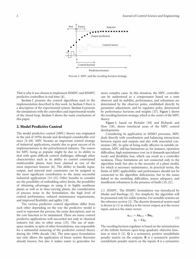
2 Journal of Control Science and Engineering
Past Future
Output prediction
Setpoint
Control moves
k
Control horizon
Prediction horizon
Figure 1: MPC and the receding horizon strategy.
That is why it was chosen to implement IHMPC and RSMPCpredictive controllers in real time [4].
Section 2 presents the control algorithms used in theimplementation described in this work. In Section 3 there isa description of the experimental system. Section 4 presentsthe simulations with the controllers and experimental resultsof the closed loop. Section 5 shows the main conclusions ofthis paper.
2. Model Predictive Control
The model predictive control (MPC) theory was originatedin the end of 1970s decade and developed considerably eversince [5–10]. MPC became an important control strategyof industrial applications, mainly due to great success of itsimplementations in the petrochemical industry. The reasonfor MPC being so popular might be due to its ability todeal with quite difficult control challenges, although othercharacteristics such as its ability to control constrainedmultivariable plants, have been claimed as one of themost important features [6]. The ability to handle input,output, and internal state constraints can be assigned asthe most significant contribution to the many successfulindustrial applications [11–13]. Other benefits to considerare the possibility of embedding safety limits, the possibilityof obtaining advantages in using it in highly nonlinearplants as well as in time-varying plants, the considerationof process noise in the formulation, the high level ofcontrol performance, reduced maintenance requirements,and improved flexibility and agility [14].
The various predictive control algorithms differ fromeach other depending on the way the predictive model isused to represent the process, the noise description, and onthe cost function to be minimized. There are many controlpredictive applications well succeeded not only in chemicalindustry but also in other areas [15]. The use of state-space models, in spite of other formulations, was responsiblefor a substantial maturing of the predictive control theoryduring the 1990s decade [16]. The state-space formulationnot only allows the application of linear system theoremsalready known, but also it makes easier to generalize for
more complex cases. In this situation, the MPC controllercan be understood as a compensator based on a stateobserver and its stability, performance, and robustness aredetermined by the observer poles, established directly byparameter adjustment, and by regulator poles, determinedby performance horizons and weights [17]. Figure 1 showsthe receding horizon strategy, which is the center of the MPCtheory.
Figure 2, based on Richalet [18] and Richards andHow [19], shows interfacial areas of the MPC controldevelopments.
Considering its application to MIMO processes, MPCdeals directly with coordination and balancing interactionsbetween inputs and outputs and also with associated con-straints [20]. In spite of being really effective in suitable sit-uations, MPC still has limitations as, for instance, operationdifficulties, high maintenance cost (as it demands specializedwork) and flexibility loss, which can result in a controllerweakness. These limitations are not connected only to thealgorithm itself, but also to the necessity of a plant model,for which is necessary maintenance. In practical terms, thelimits of MPC applicability and performance should not beconnected to the algorithm deficiencies, but to the issueslinked to the modeling difficulties, sensor adequacy, andinsufficient robustness in the presence of faults [15, 21].
2.1. IHMPC. The IHMPC formulation was introduced byMuske and Rawlings [2]. For simplicity the algorithm willbe presented only for stable systems. For unstable systems seethe reference section [2]. The discrete dynamical system usedis shown in (1) in which y is the vector output, u is the vectorinput, and x is the states vector:
xk+1 = Axk+1 + Buk,
yk = Cxk .(1)
The receding horizon regulator is based on the minimizationof the infinite horizon open-loop quadratic objective func-tion at time k (2). Q is a symmetric positive semidefinitepenalty matrix on the outputs. R is a symmetric positivesemidefinite penalty matrix on the inputs. S is a symmetric

Journal of Control Science and Engineering 3
RMPC
Optimizationof hierarchical
control
Functionalmodes
Modeling
Artificialintelligence
TrainingDiagnosis
Integratedproject
Mathematics
Computational methods
Phy
sica
l sys
tem
Bio
logi
cal s
yste
m
Hybrid MPC
MPC
Alarm Man-machineinterface
Fault-tolerantMPC
Figure 2: MPC and related areas.
Figure 3: Experimental system.
positive semidefinite penalty matrix on the rate of the inputchange with Δu = uk+i − uk. The vector uNcontains the Nfuture open-loop control moves (3). The infinite horizonopen-loop objective function can be expressed as a finite
1 2
4
3FC FT FT FC
LT
NaOH
NaHCO3
HNO3
hm
pHmpHT
Figure 4: Diagram representation of the experimental system.
horizon open-loop objective. For stable system, Q is definedas the infinite sum (4). This infinite sum can be determinedfrom the solution of the discrete Lyapunov equation (5).Using simple algebraic manipulation, the quadratic objective

4 Journal of Control Science and Engineering
0.2 0.4 0.6 0.8 1.2 1.4 1.6 1.823456789
101112
pH
q2/q1
0 21
q3 = 0 mL/sq3 = 0.05 mL/sq3 = 0.08 mL/s
q3 = 0.1 mL/s
Experimentalq3 = 0.5 mL/s
Figure 5: Titration Curves of the neutralization system.
−0.5 −0.4 −0.3 −0.2 −0.1 0 0.1 0.2 0.3 0.4 0.50
50
100
150
200
250
Freq
uen
cy e
rror
inh
Error in predicting h
Figure 6: Error in predicting the level of the reactor.
is show in (6). The matrices H, G, and F are showed in (7)–(9):
Jk = minuN
∞∑
i=0
yTk+iQyk+i + uT
k+iRuk+i + ΔuTk+iSΔuk+i, (2)
uN =
⎡⎢⎢⎢⎢⎣
uk
uk+1...
uk+N−1
⎤⎥⎥⎥⎥⎦
, (3)
Q =∞∑
i=0
AT iCTQCAi, (4)
Q = CTQC + ATQA, (5)
minΦkuN
= minuN
uNTHuN + 2uNT
(Gxk − Fuk−1), (6)
0 20 40 60 80 100 120 140 160 180 2009.5
10
10.5
11
11.5
12
12.5
13
13.5
Time (min)
u(m
L/s)
q1
q2
Figure 7: Random inputs for parameter estimation.
100 110 120 130 140 150 160 170 180 190 2006
7
8
9
10
11
12
13
Time (min)
h(c
m)
hh-Mod
Figure 8: Open-loop run behavior (Mod indicates that it is a resultof model simulation).
0 20 40 60 80 100 120 140 160 180 2002
4
6
8
10
12
14
16
18
Time (min)
Ou
tpu
t
hpH pH Mod
h Mod
Figure 9: Real data x simulated data (Mod).
H=
⎡⎢⎢⎢⎢⎢⎣
BTQB + R + 2S BTATQB− S · · · BTATN−1QB
BTQAB− S BTQB + R + 2S · · · BTATN−2QB
......
. . ....
BTQAN−1B BTQAN−2B · · · BTQB + R + 2S
⎤⎥⎥⎥⎥⎥⎦
,
(7)

Journal of Control Science and Engineering 5
Process
Transmitterh
h
pH
Filter
FilterCalibration curve
Calibration curve
Calibration curve
Calibration curve
MPC
or
RSMPC
Filter
Filter
+
+
+
Computer
−
−
−
−
+Data acquisition
Data acquisition
PID-q1
PID-q2
Transmitterq1 flow
Transmitterq2 flow
Pumpq1 (mL/s)
Pumpq2 (mL/s)
TransmitterpH
(4–20 mA)
(4–20 mA)
Software-LabviewSoftware-Matlab
HardwareProcess
hSPOutput (channel—0 to 5)
Output (channel—0 to 5)
Input (channel—0 to 15)
Input (channel—0 to 5)
pHSP
q3 (mL/s)
Figure 10: Structure of operation—experimental plant.
G =
⎡⎢⎢⎢⎢⎣
BTQABTQA2
...BTQAN
⎤⎥⎥⎥⎥⎦
, (8)
F =
⎡⎢⎢⎢⎢⎣
S0...0
⎤⎥⎥⎥⎥⎦. (9)
2.2. RSMPC. The RSMPC strategy is basically a trans-formation of an optimization problem with constraintsinto a quadratic programming problem [3]. The RSMPCdevelopment is presented next. Consider a general systemdescribed by (10). By linearizing (10) with the Taylor’s seriesexpansion around the point immediately before the currentoperational point, one obtains (11). The matrices are definedin (12)–(16). Equation (11) is integrated from t to t + Δtand by assuming uk constant between samples, one can write(17):
dxdt= f(x, u), y = h(x), (10)
dxdt= Ak−1x + Bk−1u + fk−1, y = Ck−1x + hk−1, (11)
Ak−1 =(∂f∂x
)∣∣∣∣x=xk−1, u=uk−1
, (12)
Bk−1 =(∂f∂u
)∣∣∣∣x=xk−1, u=uk−1
, (13)
Ck−1 =(∂h∂x
)∣∣∣∣x=xk−1
, (14)
fk−1 = f(x, u)|x=xk−1, u=uk−1, (15)
hk−1 = h|x=xk−1 , (16)
xk+1 = Φxk + ΨBuk + Ψfk−1,
yk = Cxk + hk−1,(17)
where
Φ = eAΔt, Ψ = A−1(eAΔt − I
)B, Ω = A−1
(eAΔt − I
).
(18)
Since A is not singular, then (17) can be written for eachprediction instant from k = 1 to k = P, where P is theprediction horizon and N is the control horizon, with P ≥ Nand Δuk+ j = 0 to N ≤ j ≤ P. The resulting set of equationis showed below, where
y = ΓΔu + γ, (19)
y =[
yk+1 yk+2 · · · yk+N · · · yk+P
], (20)
Δu =[Δuk+1 Δuk+2 · · · Δuk+N
]. (21)
The controller is designed in order to transform the closed-loop behavior in a fist-order system behavior accordingto (24). To overcome the problem of infeasible solutionsof the MPC optimization problem, a slack variable (λ) isintroduced in order to allow the system to deviate fromreference system and to satisfy hard constraints [3] resultingin (25). This equation can be written for each predictioninstant (26):

6 Journal of Control Science and Engineering
Figure 11: Frontal panel—IHMPC.

Journal of Control Science and Engineering 7
Figure 12: Block diagram—IHMPC.
0 50 100 150 200 250
4
5
6
7
8
9
10
pH (
adm
.)
Time (min)
pHpH-RefpH-SP
Figure 13: Closed-loop simulation: RSMPC—pH (setpoint: SP and reference system: Ref).
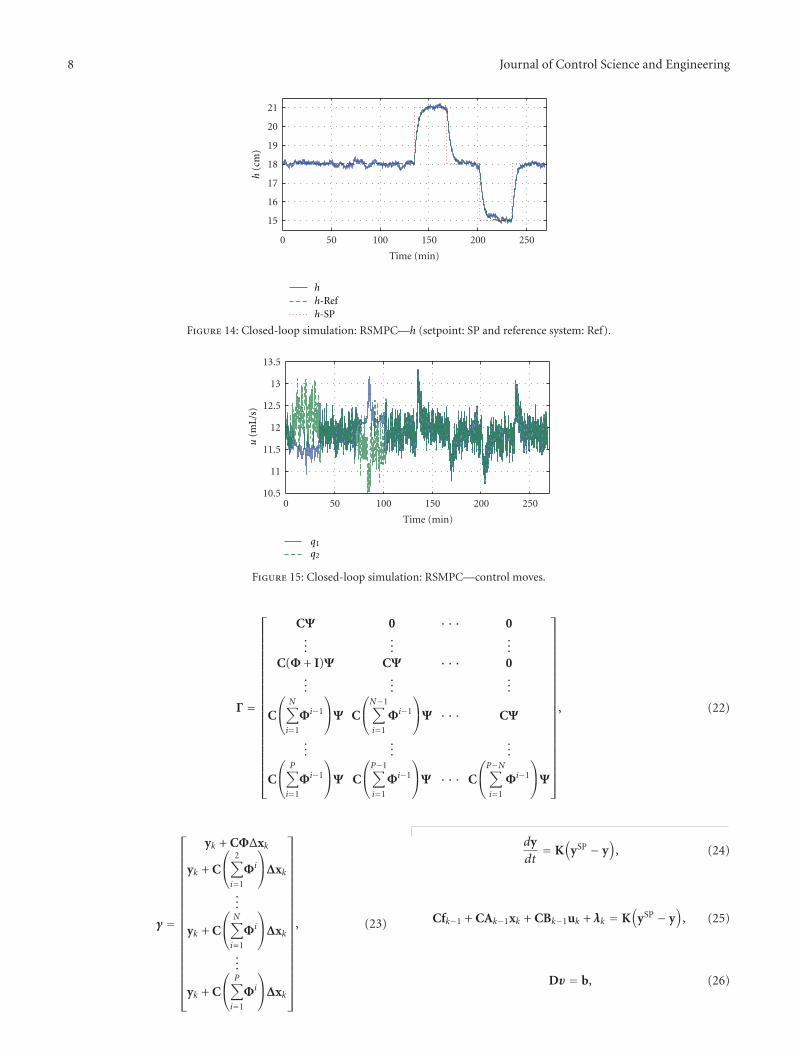
8 Journal of Control Science and Engineering
0 50 100 150 200 250
15
16
17
18
19
20
21
Time (min)
hh-Refh-SP
h(c
m)
Figure 14: Closed-loop simulation: RSMPC—h (setpoint: SP and reference system: Ref).
0 50 100 150 200 25010.5
11
11.5
12
12.5
13
13.5
Time (min)
u(m
L/s)
q1
q2
Figure 15: Closed-loop simulation: RSMPC—control moves.
Γ =
⎡⎢⎢⎢⎢⎢⎢⎢⎢⎢⎢⎢⎢⎢⎢⎢⎢⎢⎢⎢⎢⎢⎣
CΨ 0 · · · 0...
......
C(Φ + I)Ψ CΨ · · · 0...
......
C
⎛⎝
N∑
i=1
Φi−1
⎞⎠Ψ C
⎛⎝N−1∑
i=1
Φi−1
⎞⎠Ψ · · · CΨ
......
...
C
⎛⎝
P∑
i=1
Φi−1
⎞⎠Ψ C
⎛⎝P−1∑
i=1
Φi−1
⎞⎠Ψ · · · C
⎛⎝P−N∑
i=1
Φi−1
⎞⎠Ψ
⎤⎥⎥⎥⎥⎥⎥⎥⎥⎥⎥⎥⎥⎥⎥⎥⎥⎥⎥⎥⎥⎥⎦
, (22)
γ =
⎡⎢⎢⎢⎢⎢⎢⎢⎢⎢⎢⎢⎢⎢⎢⎢⎢⎢⎢⎢⎢⎣
yk + CΦΔxk
yk + C
⎛⎝
2∑
i=1
Φi
⎞⎠Δxk
...
yk + C
⎛⎝
N∑
i=1
Φi
⎞⎠Δxk
...
yk + C
⎛⎝
P∑
i=1
Φi
⎞⎠Δxk
⎤⎥⎥⎥⎥⎥⎥⎥⎥⎥⎥⎥⎥⎥⎥⎥⎥⎥⎥⎥⎥⎦
, (23)
dydt= K
(ySP − y
), (24)
Cfk−1 + CAk−1xk + CBk−1uk + λk = K(
ySP − y)
, (25)
Dυ = b, (26)
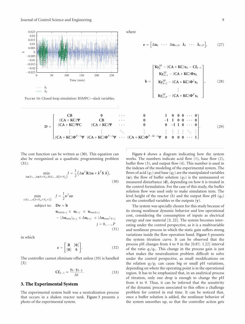
Journal of Control Science and Engineering 9
0 50 100 150 200 250−0.025
−0.02−0.015
−0.01−0.005
00.005
0.010.015
0.020.025
Time (min)
λ
λ1
λ2
Figure 16: Closed-loop simulation: RSMPC—slack variables.
where
υ =[Δuk · · · Δuk+N λk · · · λk+P
], (27)
b =
⎡⎢⎢⎢⎢⎢⎢⎢⎢⎢⎢⎣
KySPk − (CA + KC)xk − Cfk−1
KySPk+1 − (CA + KC)Φxk
KySPk+2 − (CA + KC)Φ2xk
...KySP
k+P − (CA + KC)ΦPxk
⎤⎥⎥⎥⎥⎥⎥⎥⎥⎥⎥⎦
, (28)
D =
⎡⎢⎢⎢⎢⎢⎢⎣
CB 0 · · · 0 I 0 0 0 · · · 0(CA + KC)Ψ CB · · · 0 −I I 0 0 · · · 0
(CA + KC)ΨC (CA + KC)Ψ · · · 0 0 −I I 0 · · · 0...
.... . .
......
......
.... . .
...(CA + KC)ΦP−1Ψ (CA + KC)ΦP−2Ψ · · · (CA + KC)ΦP−M−1Ψ 0 0 0 0 · · · I
⎤⎥⎥⎥⎥⎥⎥⎦. (29)
The cost function can be written as (30). This equation canalso be reorganized as a quadratic programming problem(31):
minΔu(k),...,Δu(k+Nm)λ(k),...,λ(k+Np)
J = 12
(ΔuTRΔu + λTS λ
),
(30)
minυ(k),...,υ(k+Nm+Np+2)
J = 12υTευ
subject to: Dυ = b
umink+ j ≤ uk+ j ≤ umaxk+ j
− |Δumin|k+ j ≤ Δuk+ j ≤ |Δumax| k+ j
j = 0, . . . ,P(31)
in which
ε =[
R [0][0] S
]. (32)
The controller cannot eliminate offset unless (33) is handled[3]:
Cfk−1 ≈ yk−yk−1
Δt. (33)
3. The Experimental System
The experimental system built was a neutralization processthat occurs in a shaken reactor tank. Figure 3 presents aphoto of the experimental system.
Figure 4 shows a diagram indicating how the systemworks. The numbers indicate acid flow (1), base flow (2),buffer flow (3), and output flow (4). This number is used inthe indexes of the modeling of the experimental system. Theflows of acid (q1) and base (q2) are the manipulated variables(u); the flow of buffer solution (q3) is the unmeasured ormeasured disturbance (d), depending on how it is treated inthe control formulation. For the case of this study, the buffersolution flow was used only to make simulation tests. Thelevel height of the reactor (h) and the output flow pH (q4)are the controlled variables or the outputs (y).
The system was specially chosen for this study because ofits strong nonlinear dynamic behavior and low operationalcost, considering the consumption of inputs as electricalenergy and raw material [3, 22]. The system becomes inter-esting under the control perspective, as it is a multivariableand nonlinear process in which the static gain suffers strongvariations inside the flow operation band. Figure 5 presentsthe system titration curve. It can be observed that theprocess pH changes from 4 to 9 in the [0.87; 1.22] intervalof the ratio q2/q1. This change in the process gain is justwhat makes the neutralization problem difficult to solveunder the control perspective, as small modifications onthe relation q2/q1 can cause big or small pH variations,depending on where the operating point is in the operationalregion. It has to be emphasized that, in an analytical processof titration, only one drop is enough to change the pHfrom 4 to 9. Thus, it can be inferred that the sensitivityof the dynamic process associated to this offers a challengeproblem for control in real time. It can be noticed that,once a buffer solution is added, the nonlinear behavior ofthe system smoothes up, so that the controller action gets

10 Journal of Control Science and Engineering
0 50 100 150
4
5
6
7
8
9
10
Time (min)pH
(ad
m.)
pH
pH-RefpH-SP
Figure 17: Experimental response RSMPC—pH (setpoint: SP and reference system: Ref).
0 50 100 15017.517.617.717.817.918
18.118.218.318.418.5
Time (min)
h
h-Ref
h(c
m)
h-SP
Figure 18: Experimental response: RSMPC—h (setpoint: SP and reference system: Ref).
0 50 100 15010
10.5
11
11.5
12
12.5
13
13.5
14
Time (min)
u(m
L/s)
q2q1
q1-SP q2-SP
Figure 19: Experimental response: inputs.
easier, according to what the simulation curves with thissolution indicate. If the system was linear, the relation givenby pH ×q2/q1 plots would be a line whose approximationcan be realized by the simulated curve of larger amountof buffer solution. Montandon [3] presented results for
the closed-loop system using pH control of the acid flowwith classical PID controller. The conclusion was that thisimplementation was not able to reject disturbances in asatisfactory manner. During the preparation of this work ithas been studied certain PID testing for the MIMO case,
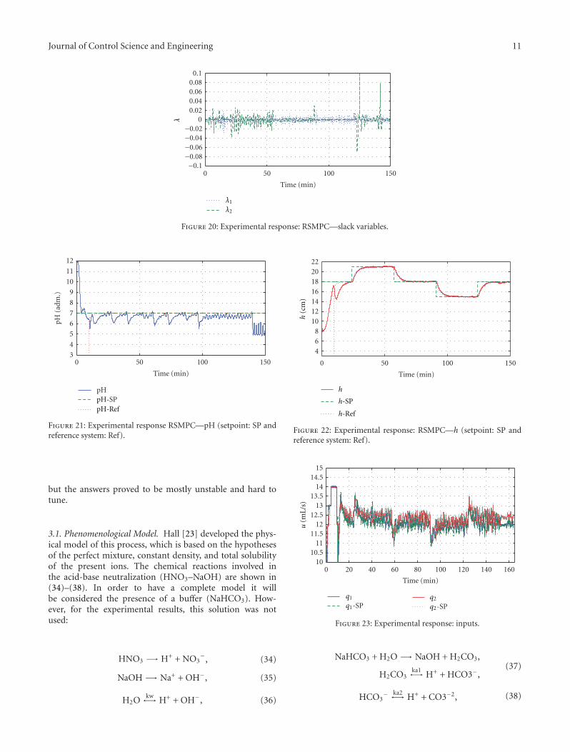
Journal of Control Science and Engineering 11
0 50 100 150−0.1
−0.08−0.06−0.04−0.02
00.020.040.060.08
0.1
Time (min)
λ1
λ2
λ
Figure 20: Experimental response: RSMPC—slack variables.
0 50 100 1503
4
5
6
7
8
9
10
11
12
Time (min)
pH (
adm
.)
pH
pH-RefpH-SP
Figure 21: Experimental response RSMPC—pH (setpoint: SP andreference system: Ref).
but the answers proved to be mostly unstable and hard totune.
3.1. Phenomenological Model. Hall [23] developed the phys-ical model of this process, which is based on the hypothesesof the perfect mixture, constant density, and total solubilityof the present ions. The chemical reactions involved inthe acid-base neutralization (HNO3–NaOH) are shown in(34)–(38). In order to have a complete model it willbe considered the presence of a buffer (NaHCO3). How-ever, for the experimental results, this solution was notused:
HNO3 −→ H+ + NO3−, (34)
NaOH −→ Na+ + OH−, (35)
H2Okw←→ H+ + OH−, (36)
0 50 100 150
468
10121416182022
Time (min)
h(c
m)
h
h-SP
h-Ref
Figure 22: Experimental response: RSMPC—h (setpoint: SP andreference system: Ref).
0 20 40 60 80 100 120 140 16010
10.511
11.512
12.513
13.514
14.515
Time (min)
u(m
L/s)
q1
q1-SPq2
q2-SP
Figure 23: Experimental response: inputs.
NaHCO3 + H2O −→ NaOH + H2CO3,
H2CO3ka1←→ H+ + HCO3−,
(37)
HCO3− ka2←→ H+ + CO3−2, (38)

12 Journal of Control Science and Engineering
0 50 100 150
−0.04
−0.02
0.02
0.04
0.06
Time (min)
λ
0
λ1
λ2
Figure 24: Experimental response: RSMPC—slack variables.
0 50 100 150 200 250
4
5
6
7
8
9
10
pH (
adm
.)
Time (min)
pHpH-SP
Figure 25: Closed-loop simulation: IHMPC-pH.
where
ka1 =⌊HCO3
−⌋⌊H+⌋
[H2CO3], (39)
ka2 =⌊CO3
−⌋⌊H+⌋[HCO3
−] . (40)
The amounts of Wa and Wb are called as invariants,because their concentrations are not affected along thereaction. The reactions are fast enough to allow the systemto be considered as in equilibrium. Then, the equilibriumreactions can be used to determine the concentration ofthe hydrogen (H) ions through the concentration of thereaction invariants. Equation (41) gives the equilibriumconcentration. According to Gustafsson and Waller [24],there are two reaction invariants defined for the ith streamand presented in (42) and (43), which, when are combined,
Table 1: System nominal parameters.
Variables Symbol Nominal values
Level H 25 cm
Area Ar 168.38 cm2
Volume Vr 4209.67 cm3
Acid flow q1 11.9130 mL/s
Base flow q2 11.8235 mL/s
Buffer solution flow q3 0.01 mL/s
pH pH 7.0
Acid conc. in q1 [HNO3] 3.510× 10−03 M
Base conc. in q2 [NaOH] 3.510× 10−03 M
result in an implicit relation of H, Wa, and Wb, as (44)shows:
kw = ⌊H+⌋⌊OH−⌋, (41)
Wai =⌊H+⌋
i −⌊OH−
⌋i −⌊HCO3
−⌋i − 2
⌊CO3
−2⌋i, (42)
Wbi = [H2CO3]i +[HCO3
−]i − 2
[CO3
−2]i, (43)
Wa = H− kwH−Wb
(ka1/H) + 2(ka1ka2)/H2
1 + (ka1/H) +(
ka1ka2/H2) . (44)
Making the mass balance in the reactor, together withthe invariant equations and considering that the density isconstant by hypothesis, will result in a differential equationsystem (45)–(47):
dh
dt= 1
Ar
(q1 + q2 + q3 − q4
), (45)
dWa
dt= 1
Vr
(q1(Wa1 −Wa) + q2(Wa2 −Wa)
+q3(Wa3 −Wa)),
(46)
dWb
dt= 1
Vr
(q1(Wb1 −Wb) + q2(Wb2 −Wb) ,
+q3(Wb3 −Wb)),
(47)
where Ar is the reactor area, Vr is the reaction volume; h isthe solution height in the reactor; Wa is the acid reactioninvariant; Wb is the base reaction invariant.
The flow output of the system is driven by gravity. Theoutput flow (q4) is done by a globe-type valve (48). Thisequation shows the relation between output flow and thereactor height and the parameters to be estimated (cv andp7). The valve parameters were estimated by using the modeland experimental data from open loop. After this processof defining the parameters of the valve it was locked so asto avoid modifying these parameters. Nominal operationconditions are presented in Table 1:
q4 = cvhp7. (48)
For estimation and validation of the model, the plantoperation must be done through the inputs that excite all thedynamic modes and in a large frequency band, so that the
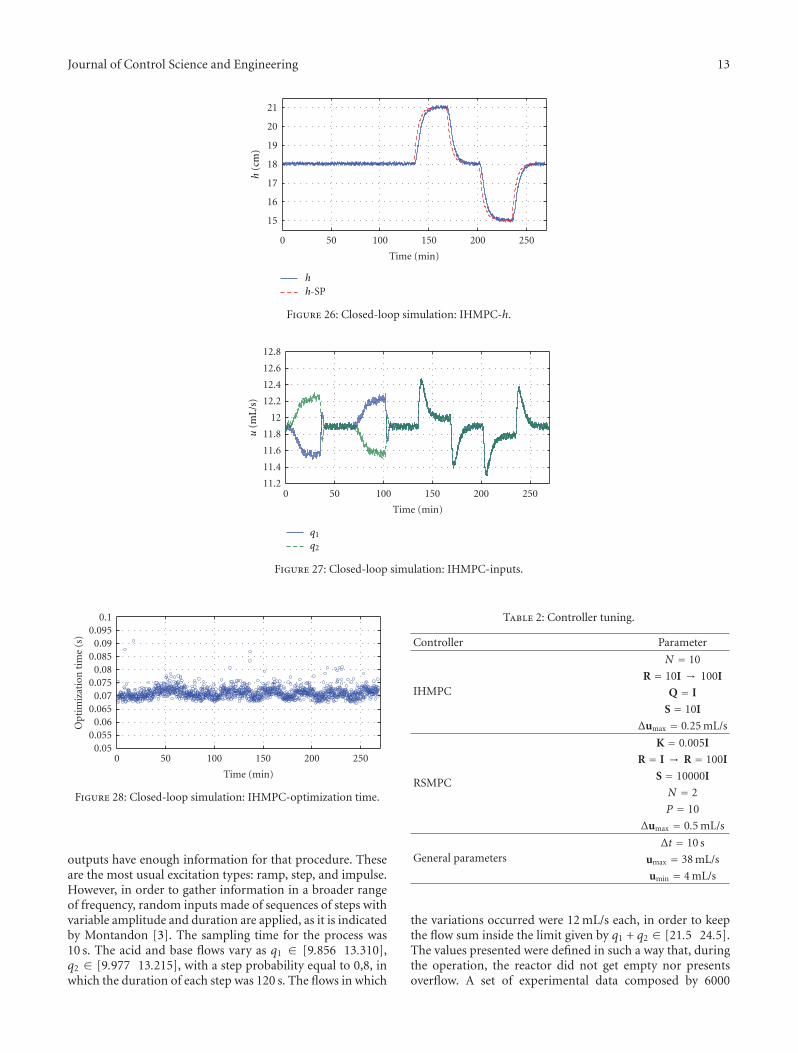
Journal of Control Science and Engineering 13
0 50 100 150 200 250
15
16
17
18
19
20
21
Time (min)h
(cm
)
h
h-SP
Figure 26: Closed-loop simulation: IHMPC-h.
0 50 100 150 200 25011.2
11.4
11.6
11.8
12
12.2
12.4
12.6
12.8
Time (min)
u(m
L/s)
q1
q2
Figure 27: Closed-loop simulation: IHMPC-inputs.
0 50 100 150 200 2500.05
0.0550.06
0.0650.07
0.0750.08
0.0850.09
0.0950.1
Time (min)
Opt
imiz
atio
n t
ime
(s)
Figure 28: Closed-loop simulation: IHMPC-optimization time.
outputs have enough information for that procedure. Theseare the most usual excitation types: ramp, step, and impulse.However, in order to gather information in a broader rangeof frequency, random inputs made of sequences of steps withvariable amplitude and duration are applied, as it is indicatedby Montandon [3]. The sampling time for the process was10 s. The acid and base flows vary as q1 ∈ [9.856 13.310],q2 ∈ [9.977 13.215], with a step probability equal to 0,8, inwhich the duration of each step was 120 s. The flows in which
Table 2: Controller tuning.
Controller Parameter
IHMPC
N = 10
R = 10I → 100I
Q = I
S = 10I
Δumax = 0.25 mL/s
RSMPC
K = 0.005I
R = I → R = 100I
S = 10000I
N = 2
P = 10
Δumax = 0.5 mL/s
General parametersΔt = 10 s
umax = 38 mL/s
umin = 4 mL/s
the variations occurred were 12 mL/s each, in order to keepthe flow sum inside the limit given by q1 + q2 ∈ [21.5 24.5].The values presented were defined in such a way that, duringthe operation, the reactor did not get empty nor presentsoverflow. A set of experimental data composed by 6000

14 Journal of Control Science and Engineering
0 20 40 60 80 100 1206.56.66.76.86.9
77.17.27.37.47.5
Time (min)pH
(ad
m.)
pHpH-SP
Figure 29: Experimental response: IHMPC-pH.
0 20 40 60 80 100 12014
15
16
17
18
19
20
21
Time (min)
h(c
m)
hh-SP
Figure 30: Experimental response: IHMPC-h.
acquisition points was used. The estimation procedure usedhalf of the data and the validation employed the remainingdata, in order to assure that the model would have the abilityfor predicting unknown data. The estimation is a nonlinearsolution of the approximation curve that uses the least squaremethod with a first trial given by a random value and astep equal to 15. The estimated values that resulted werecv = 20.4477 and p7 = 0.0523. Figure 6 shows the errorin predicting h. Figure 7 presents the set of input randomdata. Figure 8 presents the results of the simulation and theexperimental ones for the closed-loop run, in which one cannotice that the model is very representative of the process,with difficulties to predict around pH 7; this phenomenonwas already expected, taking into account the titration curveof the system. Figure 9 shows the validation of the modelby the prediction of the output that comes very close to theexperimental data.
3.2. State-Space Model. The state-space approach resultingfrom the algebraic manipulation is given by (49)–(55). Theterms dWadz and dWbdz are defined in (56) and (57).Equation (58) presents dydz relation:
x =[h Wa Wb
], (49)
u =[q1 q2
], (50)
y =[h pH
], (51)
d = [q3], (52)
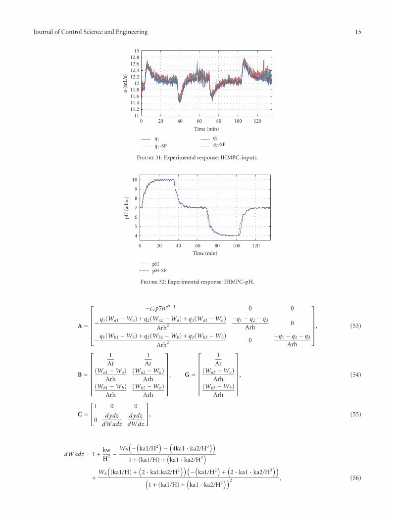
Journal of Control Science and Engineering 15
0 20 40 60 80 100 12011
11.211.411.611.8
1212.212.412.612.8
13
Time (min)u
(mL/
s)
q1 q2
q1-SP q2-SP
Figure 31: Experimental response: IHMPC-inputs.
0 20 40 60 80 100 120
4
5
6
7
8
9
10
Time (min)
pH (
adm
.)
pHpH-SP
Figure 32: Experimental response: IHMPC-pH.
A =
⎡⎢⎢⎢⎢⎢⎢⎣
−cv p7hp7−1 0 0
−q1(Wa1 −Wa) + q2(Wa2 −Wa) + q3(Wa3 −Wa)
Arh2
−q1 − q2 − q3
Arh0
−q1(Wb1 −Wb) + q2(Wb2 −Wb) + q3(Wb3 −Wb)
Arh2 0−q1 − q2 − q3
Arh
⎤⎥⎥⎥⎥⎥⎥⎦
, (53)
B =
⎡⎢⎢⎢⎢⎢⎢⎢⎣
1Ar
1Ar
(Wa1 −Wa)Arh
(Wa2 −Wa)Arh
(Wb1 −Wb)Arh
(Wb2 −Wb)Arh
⎤⎥⎥⎥⎥⎥⎥⎥⎦
, G =
⎡⎢⎢⎢⎢⎢⎢⎢⎣
1Ar
(Wa3 −Wa)Arh
(Wb3 −Wb)Arh
⎤⎥⎥⎥⎥⎥⎥⎥⎦
, (54)
C =⎡⎢⎣
1 0 0
0dydz
dWadz
dydz
dWdz
⎤⎥⎦, (55)
dWadz = 1 +kwH2 −
Wb
(−(
ka1/H2)−(
4ka1 · ka2/H3))
1 + (ka1/H) +(
ka1 · ka2/H2)
+Wb
((ka1/H) +
(2 · ka1.ka2/H2
))(−(
ka1/H2)
+(
2 · ka1 · ka2/H3))
(1 + (ka1/H) +
(ka1 · ka2/H2
))2 , (56)
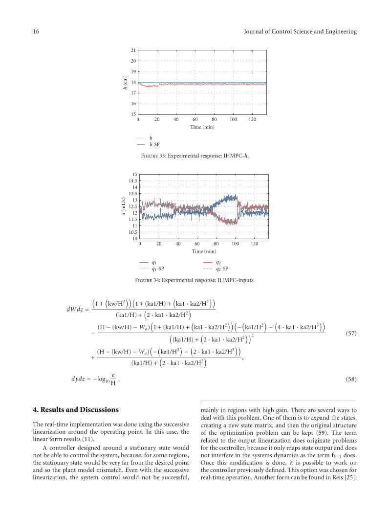
16 Journal of Control Science and Engineering
0 20 40 60 80 100 12015
16
17
18
19
20
21
Time (min)
h
h(c
m)
h-SP
Figure 33: Experimental response: IHMPC-h.
0 20 40 60 80 100 12010
10.511
11.512
12.513
13.514
14.515
Time (min)
u(m
L/s)
q1
q1-SPq2
q2-SP
Figure 34: Experimental response: IHMPC-inputs.
dWdz =(
1 +(
kw/H2))(
1 + (ka1/H) +(
ka1 · ka2/H2))
(ka1/H) +(
2 · ka1 · ka2/H2)
−(H− (kw/H)−Wa)
(1 + (ka1/H) +
(ka1 · ka2/H2
))(−(
ka1/H2)−(
4 · ka1 · ka2/H3))
((ka1/H) +
(2 · ka1 · ka2/H2
))2
+(H− (kw/H)−Wa)
(−(
ka1/H2)−(
2 · ka1 · ka2/H3))
(ka1/H) +(
2 · ka1 · ka2/H2) ,
(57)
dydz = −log10e
H. (58)
4. Results and Discussions
The real-time implementation was done using the successivelinearization around the operating point. In this case, thelinear form results (11).
A controller designed around a stationary state wouldnot be able to control the system, because, for some regions,the stationary state would be very far from the desired pointand so the plant model mismatch. Even with the successivelinearization, the system control would not be successful,
mainly in regions with high gain. There are several ways todeal with this problem. One of them is to expand the states,creating a new state matrix, and then the original structureof the optimization problem can be kept (59). The termrelated to the output linearization does originate problemsfor the controller, because it only maps state output and doesnot interfere in the systems dynamics as the term fk−1 does.Once this modification is done, it is possible to work onthe controller previously defined. This option was chosen forreal-time operation. Another form can be found in Reis [25]:
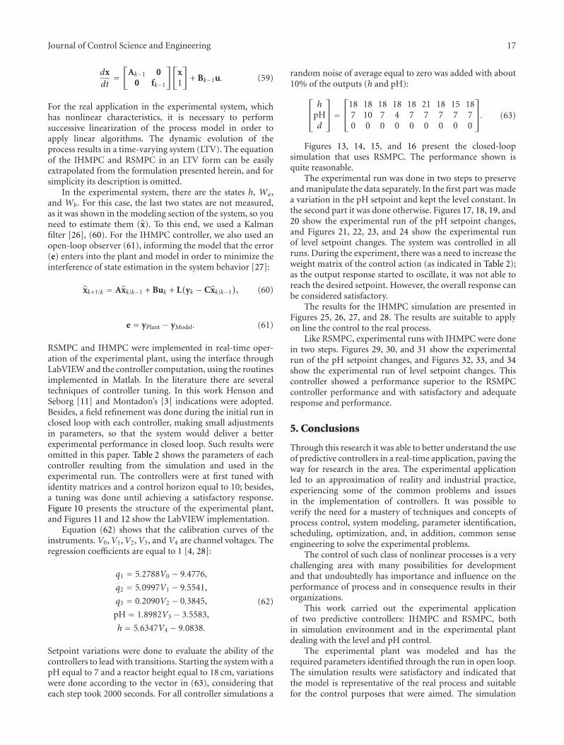
Journal of Control Science and Engineering 17
dxdt=[
Ak−1 00 fk−1
][x1
]+ Bk−1u. (59)
For the real application in the experimental system, whichhas nonlinear characteristics, it is necessary to performsuccessive linearization of the process model in order toapply linear algorithms. The dynamic evolution of theprocess results in a time-varying system (LTV). The equationof the IHMPC and RSMPC in an LTV form can be easilyextrapolated from the formulation presented herein, and forsimplicity its description is omitted.
In the experimental system, there are the states h, Wa,and Wb. For this case, the last two states are not measured,as it was shown in the modeling section of the system, so youneed to estimate them (x). To this end, we used a Kalmanfilter [26], (60). For the IHMPC controller, we also used anopen-loop observer (61), informing the model that the error(e) enters into the plant and model in order to minimize theinterference of state estimation in the system behavior [27]:
xk+1|k = Axk|k−1 + Buk + L(
yk − Cxk|k−1), (60)
e = yPlant − yModel. (61)
RSMPC and IHMPC were implemented in real-time oper-ation of the experimental plant, using the interface throughLabVIEW and the controller computation, using the routinesimplemented in Matlab. In the literature there are severaltechniques of controller tuning. In this work Henson andSeborg [11] and Montadon’s [3] indications were adopted.Besides, a field refinement was done during the initial run inclosed loop with each controller, making small adjustmentsin parameters, so that the system would deliver a betterexperimental performance in closed loop. Such results wereomitted in this paper. Table 2 shows the parameters of eachcontroller resulting from the simulation and used in theexperimental run. The controllers were at first tuned withidentity matrices and a control horizon equal to 10; besides,a tuning was done until achieving a satisfactory response.Figure 10 presents the structure of the experimental plant,and Figures 11 and 12 show the LabVIEW implementation.
Equation (62) shows that the calibration curves of theinstruments. V0,V1,V2,V3, and V4 are channel voltages. Theregression coefficients are equal to 1 [4, 28]:
q1 = 5.2788V0 − 9.4776,
q2 = 5.0997V1 − 9.5541,
q3 = 0.2090V2 − 0.3845,
pH = 1.8982V3 − 3.5583,
h = 5.6347V4 − 9.0838.
(62)
Setpoint variations were done to evaluate the ability of thecontrollers to lead with transitions. Starting the system with apH equal to 7 and a reactor height equal to 18 cm, variationswere done according to the vector in (63), considering thateach step took 2000 seconds. For all controller simulations a
random noise of average equal to zero was added with about10% of the outputs (h and pH):
⎡⎢⎣
hpHd
⎤⎥⎦ =
⎡⎢⎣
18 18 18 18 18 21 18 15 187 10 7 4 7 7 7 7 70 0 0 0 0 0 0 0 0
⎤⎥⎦. (63)
Figures 13, 14, 15, and 16 present the closed-loopsimulation that uses RSMPC. The performance shown isquite reasonable.
The experimental run was done in two steps to preserveand manipulate the data separately. In the first part was madea variation in the pH setpoint and kept the level constant. Inthe second part it was done otherwise. Figures 17, 18, 19, and20 show the experimental run of the pH setpoint changes,and Figures 21, 22, 23, and 24 show the experimental runof level setpoint changes. The system was controlled in allruns. During the experiment, there was a need to increase theweight matrix of the control action (as indicated in Table 2);as the output response started to oscillate, it was not able toreach the desired setpoint. However, the overall response canbe considered satisfactory.
The results for the IHMPC simulation are presented inFigures 25, 26, 27, and 28. The results are suitable to applyon line the control to the real process.
Like RSMPC, experimental runs with IHMPC were donein two steps. Figures 29, 30, and 31 show the experimentalrun of the pH setpoint changes, and Figures 32, 33, and 34show the experimental run of level setpoint changes. Thiscontroller showed a performance superior to the RSMPCcontroller performance and with satisfactory and adequateresponse and performance.
5. Conclusions
Through this research it was able to better understand the useof predictive controllers in a real-time application, paving theway for research in the area. The experimental applicationled to an approximation of reality and industrial practice,experiencing some of the common problems and issuesin the implementation of controllers. It was possible toverify the need for a mastery of techniques and concepts ofprocess control, system modeling, parameter identification,scheduling, optimization, and, in addition, common senseengineering to solve the experimental problems.
The control of such class of nonlinear processes is a verychallenging area with many possibilities for developmentand that undoubtedly has importance and influence on theperformance of process and in consequence results in theirorganizations.
This work carried out the experimental applicationof two predictive controllers: IHMPC and RSMPC, bothin simulation environment and in the experimental plantdealing with the level and pH control.
The experimental plant was modeled and has therequired parameters identified through the run in open loop.The simulation results were satisfactory and indicated thatthe model is representative of the real process and suitablefor the control purposes that were aimed. The simulation

18 Journal of Control Science and Engineering
answers of the system outputs subjected to the controllerswere adequate and satisfactory. The theoretical and experi-mental responses of the IHMPC runs were satisfactory.
The controller adjustment for real-time operations wassuitable and feasible. The interference of matters related toleaking, process noises, and noises from electrical source andother problems associated to real-time application broughtadditional difficulties that demanded process knowledge ofthe process.
The experimental application of robust controllers asso-ciated or not to control systems tolerant to failures and theuse of online identification employing neural networks willbe presented elsewhere.
References
[1] G. Stephanopoulos, Chemical Process Control: An Introductionto Theory and Practice, Prentice Hall, Upper Saddle River, NJ,USA, 1984.
[2] K. R. Muske and J. B. Rawlings, “Model predictive control withlinear models,” AIChE Journal, vol. 39, no. 2, pp. 262–287,1993.
[3] A. G. Montandon, Controle preditivo em tempo real com tra-jetoria de referencia baseado em modelo neural para reator deneutralizacao, M.S. thesis, Federal University of Uberlandia,2005.
[4] C. H. F. Silva, Uma contribuicao ao estudo de controladoresrobustos, Ph.D. thesis, Universidade Federal de Uberlandia ,2009.
[5] E. F. Camacho and C. Bordons, Model Predictive Control,Springer, Barcelona, Spain, 1999.
[6] D. Q. Mayne, J. B. Rawlings, C. V. Rao, and P. O. M. Scokaert,“Constrained model predictive control: stability and optimal-ity,” Automatica, vol. 36, no. 6, pp. 789–814, 2000.
[7] M. Nikolaou, “Model predictive controllers: a critical synthesisof theory and industrial needs,” Advances in Chemical Engi-neering, vol. 26, pp. 131–204, 2001.
[8] M. Morari, “Model predictive control: multivariable controltechnique of choice in the 1990?” Tech. Rep. CIT/CDS 93-024,California Institute Of Technology, 1993.
[9] D. R. Saffer II and F. J. Doyle III, “Analysis of linear program-ming in model predictive control,” Computers and ChemicalEngineering, vol. 28, no. 12, pp. 2749–2763, 2004.
[10] J. B. Rawlings, “Tutorial: model predictive control technology,”in Proceedings of the American Control Conference (ACC’99),pp. 662–676, June 1999.
[11] M. A. Henson and D. E. Seborg, Nonlinear Process Control,Prentice Hall, Upper Saddle River, NJ, USA, 1997.
[12] S. de Oliveira and M. Morari, “Robust model predictive con-trol for nonlinear systems with constraints,” in Advanced Con-trol Of Chemical Processes, pp. 295–300, Kyoto, Japan, 1994.
[13] J. H. Lee, “Recent advances in model predictive control andother related areas,” AIChE Symposium Series, pp. 201–216,1997.
[14] J. W. Eaton and J. B. Rawlings, “Model-predictive control ofchemical processes,” Chemical Engineering Science, vol. 47, no.4, pp. 705–720, 1992.
[15] S. J. Qin and T. A. Badgwell, “A survey of industrial modelpredictive control technology,” Control Engineering Practice,vol. 11, no. 7, pp. 733–764, 2003.
[16] J. Lofberg, Minimax approaches to robust model predictivecontrol, Ph.D. thesis, Linkoping, Sweden, 2003.
[17] N. L. Ricker, “Model predictive control with state estimation,”Industrial and Engineering Chemistry Research, vol. 29, no. 3,pp. 374–382, 1990.
[18] J. Richalet, “Industrial applications of model based predictivecontrol,” Automatica, vol. 29, no. 5, pp. 1251–1274, 1993.
[19] A. Richards and J. How, “Robust model predictive control withimperfect information,” in Proceedings of the American ControlConference, (ACC’05), pp. 268–273, June 2005.
[20] Q. L. Zhang and Y. G. Xi, “An efficient model predictivecontroller with pole placement,” Information Sciences, vol. 178,no. 3, pp. 920–930, 2008.
[21] M. Morari and J. H. Lee, “Model predictive control: past,present and future,” Computers and Chemical Engineering, vol.23, no. 4-5, pp. 667–682, 1999.
[22] H. M. Henrique, Uma contribuicao ao estudo de redes neuronaisaplicadas ao controle de processos, Ph.D. thesis, COPPE/UFRJ,1999.
[23] R. C. Hall, Development of a multivariable pH experiment, M.S.thesis, University of California, Santa Barbara, Calif, USA,1987.
[24] T. K. Gustafsson and K. V. Waller, “Dynamic modeling andreaction invariant control of pH,” Chemical Engineering Sci-ence, vol. 38, no. 3, pp. 389–398, 1983.
[25] L. L. G. Reis, Controle tolerante com reconfiguracao estruturalacoplado a sistema de diagnostico de falhas, M.S. thesis, FederalUniversity of Uberlandia, 2008.
[26] T. Kailath, Linear Systems, Prentice Hall, Englewood Cliffs, NJ,USA, 1980.
[27] J. M. Maciejowski, Predictive Control With Constraints, Pear-son Education Limited, 2002.
[28] D. Goncalves, Controle preditivo em tempo real de uma plantapiloto, M. Sc qualification report, Federal University ofUberlandia, 2007.

Hindawi Publishing CorporationJournal of Control Science and EngineeringVolume 2012, Article ID 485784, 7 pagesdoi:10.1155/2012/485784
Research Article
Robust Model Predictive Control Using Linear MatrixInequalities for the Treatment of Asymmetric Output Constraints
Mariana Santos Matos Cavalca,1 Roberto Kawakami Harrop Galvao,2
and Takashi Yoneyama2
1 Departamento de Engenharia Eletrica, Centro de Ciencias Tecnologicas, Universidade do Estado de Santa Catarina,Praca Rua Paulo Malschitzki, Zona Industrial Norte, 89.219-710 Joinville, SC, Brazil
2 Divisao de Engenharia Eletronica, Instituto Tecnologico de Aeronautica, Praca Marechal Eduardo Gomes, 50 Vila das Acacias,12.228-900 Sao Jose dos Campos, SP, Brazil
Correspondence should be addressed to Mariana Santos Matos Cavalca, [email protected]
Received 30 June 2011; Revised 22 September 2011; Accepted 6 October 2011
Academic Editor: Marcin T. Cychowski
Copyright © 2012 Mariana Santos Matos Cavalca et al. This is an open access article distributed under the Creative CommonsAttribution License, which permits unrestricted use, distribution, and reproduction in any medium, provided the original work isproperly cited.
One of the main advantages of predictive control approaches is the capability of dealing explicitly with constraints on themanipulated and output variables. However, if the predictive control formulation does not consider model uncertainties, then theconstraint satisfaction may be compromised. A solution for this inconvenience is to use robust model predictive control (RMPC)strategies based on linear matrix inequalities (LMIs). However, LMI-based RMPC formulations typically consider only symmetricconstraints. This paper proposes a method based on pseudoreferences to treat asymmetric output constraints in integrating SISOsystems. Such technique guarantees robust constraint satisfaction and convergence of the state to the desired equilibrium point. Acase study using numerical simulation indicates that satisfactory results can be achieved.
1. Introduction
Model-based predictive control (MPC) is a strategy in whicha sequence of control actions is obtained by minimizing acost function considering the predictions of a process modelwithin a certain prediction horizon. At each sample time,only the first value of this sequence is applied to the plant,and the optimization is repeated in order to use feedbackinformation [1, 2]. One of the main advantages of MPC is thepossibility to consider explicitly the physical and operationalconstraints of the system during the design of the controlloop [1–3]. However, if there are mismatches between thenominal model and the actual behavior of the process, thenthe performance of the control loop can be degraded and theoptimization problem may even become unfeasible. Thus,the study of new strategies for design of robust MPC(RMPC) with guaranteed stability and constraint satisfactionproperties even in the presence of uncertainties is an areawith great potential for research [4–7].
In this context, Kothare et al. [7] proposed an RMPCstrategy with infinite horizon employing linear matrix in-equalities (LMIs) for dealing with model uncertainty andsymmetric constraints on the manipulated and output vari-ables. This approach was later extended to encompass mul-timodel representations [8, 9], setpoint management [10],integrator resetting [11], and offline solutions [12, 13].
Within this scope, Cavalca et al. [4] proposed a heuristicprocedure that allows the inclusion of asymmetric con-straints on the plant output, but without stability or con-straint satisfaction guarantees. The present paper presentsa formal strategy to handle asymmetric output constraintsin the control of integrating single input, single output(SISO) systems, for the case where the output is linearin states. It is shown that robust constraint satisfaction isachieved, as well as convergence of the state trajectory tothe desired equilibrium point. The effectiveness of the pro-posed method is illustrated by means of numerical simula-tions.

2 Journal of Control Science and Engineering
The remainder of this paper is organized as follows.Section 2 reviews the design of RMPC based on LMI.Section 3 formalizes the proposed technique for the inclusionof asymmetric constraints. Section 4 presents a case studyconsisting of a discrete time model of a double integrator.The results are evaluated through numerical simulations aspresented in Section 5. Concluding remarks are presented inSection 6.
Throughout the text, I represents an identity matrix,the notation (· | k) is used in predictions with respect totime k, and the ∗ superscript indicates an optimal solution.For brevity of notation, only the upper triangular part ofsymmetric matrices is explicitly presented.
2. LMI-Based RMPC
Consider a linear time-invariant system described by an un-certain model of the following form:
x(k + 1) = Ax(k) + Bu(k),
y(k) = Cx(k),(1)
where x(k) ∈ Rn, u(k) ∈ Rp, and y(k) ∈ Rq are thestates, the manipulated and the output variables, respectively,for each time k, and A, B, and C are constant matrices ofappropriate dimensions. The uncertainty is represented inpolytopic form; that is, matrices A and B are unknown to thedesigner, but they are assumed to belong to a convex polytopeΩ with L known vertices (Ai,Bi), i = 1, 2, . . . ,L, so that [2, 7]:
(A,B) =L∑
i=1
λi(Ai,Bi) (2)
for some unknown set of coefficients λ1, λ2, . . . , λL that satisfy
L∑
i=1
λi = 1 λi ≥ 0, i = 1, . . . ,L. (3)
At each time k, the sequence of future controls U∞ ={u(k | k),u(k+1 | k),u(k+2 | k), . . .} is obtained as solutionof the following min-max optimization problem:
minU∞
max(A,B)∈Ω
J∞(A,B,U∞), (4)
where
J∞(A,B,U∞) =∞∑
j=0
[∥∥x(k + j | k)∥∥2Wx
+∥∥u(k + j | k)∥∥2
Wu
]
(5)
in which Wx > 0 and Wu > 0 are symmetric weightingmatrices. By assumption, all states are available for feedbackso that x(k | k) = x(k).
This min-max problem can be replaced with the fol-lowing convex optimization problem with variables γ ∈ R,Q ∈ Rn×n, Σ ∈ Rp×n, and LMI constraints [2, 7]:
minγ,Q,Σ
γ (6)
subject to
⎡⎣Q x(k)
· 1
⎤⎦ > 0, (7)
⎡⎢⎢⎢⎢⎢⎢⎣
Q 0 0 AiQ + BiΣ
· γI 0 W1/2x Q
· · γI W1/2u Σ
· · · Q
⎤⎥⎥⎥⎥⎥⎥⎦> 0, i = 1, 2, . . . ,L.
(8)
If the problem (6)–(8) has a solution γ∗k , Q∗k , Σ∗k , thenthe optimal control sequence is given by
u(k + j | k) = K∗k x
(k + j | k), (9)
where
K∗k = Σ∗k(Q∗k)−1
. (10)
Symmetric constraints on the manipulated variables ofthe form |ul(k + j | k)| < ul, l = 1, 2, . . . , p, j ≥ 0 and on theoutput variables of the form |ym(k + j + 1 | k)| < ym, m =1, 2, . . . , q, j ≥ 0 can be imposed by including additionalLMIs [7]
⎡⎣X Σ
· Q
⎤⎦ > 0 (11)
with
Xll < ul2, l = 1, 2, . . . , p,
⎡⎣Q [AiQ + BiΣ]TCT
m
· y2m
⎤⎦ > 0, i = 1, 2, . . . ,L
(12)
for m = 1, 2, . . . , q, where Cm denotes the mth row of C.Let P(x(k)) denote the optimization problem (6) with
constraints (7), (8), (11), and (12). Suppose that the controllaw uses the concept of receding horizon; that is, u(k) =K∗k x(k) with K∗k recalculated at each sampling time k. Thefollowing lemma is concerned with convergence of the statetrajectory to the origin under the constraints imposed on theoperation of the plant.
Lemma 1. If P(x(k0)) is feasible at some time k = k0, then‖x(k)‖ → 0 as k → ∞ with satisfaction of the input andoutput constraints.
The proof of Lemma 1 follows directly from the recursivefeasibility and asymptotic stability properties demonstratedin [7].

Journal of Control Science and Engineering 3
Remark 2. As shown in Appendix A of Kothare et al. [7],P(x(k)) is equivalent to minimizing a function V(x(k | k)) =x(k | k)TPkx(k | k) with Pk = γ∗k (Q∗k )−1 > 0. Such V(x(k |k)) function is found to be an upper bound for the costfunction J∞(A,B,U∞) in (5) and can be used as a candidateLyapunov function in the proof of asymptotic stability.
Remark 3. For a regulation problem around a point differentfrom the origin, a change of variables can be used, so that thenew origin corresponds to the desired equilibrium point[7]. In the present work, the new value for the referencesignal will be termed a pseudoreference. It is assumed thatthe process is integrating, and, therefore, the control value insteady state (uss) is zero for any value of the pseudoreference.Otherwise, the determination of uss would not be trivialsince the system matrices A and B are subjected to modeluncertainties.
Remark 4. The RMPC problem formulation presented inthis section considers that the matrices A and B are unknownbut dot not vary with time. This is a particular case of thegeneral framework introduced in [7], which was concernedwith time-varying matrices A(k) and B(k).
3. Treatment of Asymmetric Constraints
The present work is concerned with regulation problemsaround the origin involving a SISO system with output vari-able y(k) = Cx(k). This is a particular case of the problemdescribed in Section 2, with p = q = 1. Therefore, theindexes l and m in (12) can be omitted. Moreover, the systemis assumed to be integrating, so that uss = 0 regardless ofthe pseudoreference, as discussed in Remark 3. It is alsoconsidered that the manipulated variable u(k) is subjectedto a symmetric constraint u as in Section 2. Suppose that theconstraints on y are of the following form:
ymin < y(k) < ymax (13)
with ymin < 0 and ymax > 0. If |ymin| = ymax, then thesymmetric constraint formulation presented in Section 2 canbe applied directly by making y = ymax. If |ymin| /= ymax, adifferent approach is required. One alternative is to adopt amore conservative constraint, that is,
y =⎧⎨⎩ymax, if ymax <
∣∣ymin∣∣
−ymin, if ymax >∣∣ymin
∣∣.(14)
However, this procedure may not be convenient in thefollowing cases:
(i) ymax < |ymin| with ymin ≤ y(k) < −ymax,
(ii) ymax > |ymin| with −ymin < y(k) ≤ ymax.
In these cases, the initial value of the output is admissibleunder the original asymmetric constraints, but not under themore conservative constraint (14). Figure 1(a) provides anillustration for case (i). As can be seen, the imposition of the
more conservative constraint −ymax < y(k) < ymax makesthe output variable y(k) be located outside of the range ofadmissible values.
Cavalca et al. [4] proposed a heuristic solution, based ona time-varying pseudoreference r(k) = min{(ymax + y(k))/2, 0} as shown in Figure 1(b). The problem of asymmetricoutput constraints is then redefined in terms of new sym-metric constraints (a/a) around r(k). However, it shouldbe noted that this technique does not lead to guaranteedstability and constraint satisfaction.
Unlike the approach described above, which involves apseudoreference r(k) that may change at each sampling timek, the solution proposed in the present paper employs asequence of pseudoreferences ri (i = 1, 2, . . . , imax) whichare defined at k = 0 on the basis of the initial outputvalue y(0). As illustrated in Figure 2, symmetric constraints(a/a, b/b, c/c, . . .) are established around each pseudorefer-ence. It will be shown that the use of such pseudoreferences,together with a convenient commutation rule, provides ro-bust constraint satisfaction and ensures that the state tra-jectory converges to the origin. For sake of brevity of pres-entation, only case (i) will be treated. Case (ii) can be recastinto case (i) by defining y(k) = −Cx(k) and replacingconstraints ymin ≤ y(k) ≤ ymax with −ymax ≤ y(k) ≤ −ymin.
Given an initial state x(0) such that y(0) = Cx(0) fallswithin the scope of case (i), the following algorithm definesthe pseudoreferences ri, as well as a sequence of associatedmatrices Q∗i . These matrices will be subsequently employedin the control law to establish a rule of commutation fromone pseudoreference to the next.
It is assumed that the setXs of possible equilibrium valuesxs for the state of the plant is known from the physics of theprocess to be controlled.
Algorithm for Determination of the Pseudoreferences andAssociated Ellipsoids (PR Algorithm).
Step 1. Define the pseudoreferences ri as follows:
Step 1.1. Let r0 = [ymax + y(0)]/2
Step 1.2. Let i = 1
Step 1.3. While |ri−1| > ymax do
ri = (ymax + ri−1)/2
i = i + 1
End While
Step 1.4. Let imax = i
Step 1.5. Let rimax = 0.
Step 2. For each ri determine xs,i such that:
Cxs,i = ri, (15)
xs,i ∈ Xs. (16)
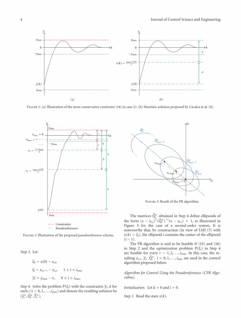
4 Journal of Control Science and Engineering
y
0
ymax
−ymax
ymin
k
y(k)
(a)
y
y(k)
0
ymax
−ymax
ymin
k
r(k) = ymax+y(k)2
a
a
(b)
Figure 1: (a) Illustration of the more conservative constraint (14) in case (i). (b) Heuristic solution proposed by Cavalca et al. [4].
k
y
ymax
· · ·rimax−1 = · · ·
rimax = 0
r2 = r1+ymax2
r1 = ymax+y(0)2
y(0)
c
b
a
c
b
a
−ymax
ConstraintsPseudoreferences
ymin
Figure 2: Illustration of the proposed pseudoreference scheme.
Step 3. Let
ξ0 = x(0)− xs,0
ξi = xs,i−1 − xs,i, 1 ≤ i ≤ imax
yi = ymax − ri, 0 ≤ i ≤ imax.
Step 4. Solve the problem P(ξi) with the constraints yi, u foreach i (i = 0, 1, . . . , imax) and denote the resulting solution by(γ∗i , Q∗i , Σ∗i ).
x1
x2
˜Q∗1
˜Q∗imax−2
˜Q∗imax−1
˜Q∗imaxxs,imax−1
· · ·
· · ·
· · ·· · ·
xs,imax−2
xs,imax = 0
Figure 3: Result of the PR algorithm.
The matrices Q∗i obtained in Step 4 define ellipsoids ofthe form (x − xs,i)
T(Q∗i )−1(x − xs,i) < 1, as illustrated inFigure 3 for the case of a second-order system. It isnoteworthy that, by construction (in view of LMI (7) withx(k) = ξi), the ellipsoid i contains the center of the ellipsoid(i− 1).
The PR algorithm is said to be feasible if (15) and (16)in Step 2 and the optimization problem P(ξi) in Step 4are feasible for every i = 1, 2, . . . , imax. In this case, the re-sulting xs,i, yi, Q∗i , i = 0, 1, . . . , imax are used in the controlalgorithm proposed below.
Algorithm for Control Using the Pseudoreferences (CPR Algo-rithm).
Initialization. Let k = 0 and i = 0.
Step 1. Read the state x(k).

Journal of Control Science and Engineering 5
Step 2. If i < imax then
Let xi+1(k) = x(k)− xi+1,s
If xTi+1(k)(Q∗i+1)−1xi+1(k) < 1 (condition of transi-tion) then
Let i = i + 1
End If
End If.
Step 3. Let xi(k) = x(k) − xs,i and solve the problemP(xi(k)) with the constraints yi and u in order to obtain(γ∗k , Q∗k , Σ∗k ).
Step 4. Calculate K∗k = Σ∗k (Q∗k )−1 and u(k) = K∗k xi(k).
Step 5. Apply u(k) to the plant.
Step 6. Let k = k+1, wait a sample time and return to Step 1.
The main result of this work is stated in the following the-orem, which is concerned with the satisfaction of constraintsand convergence of the state trajectory to the origin underthe control law given by the CPR algorithm.
Theorem 5. If the PR algorithm is feasible and the CPRalgorithm is applied to control the plant, then ‖x(k)‖ → 0 ask → ∞, with satisfaction of the input and output constraints.
Proof. For k = 0, the state x(k) lies in the ellipsoid associatedwith Q∗0 , which was obtained by solving problem P(x(0) −xs,0) in the PR algorithm. Therefore, problem P(x0(0))is feasible by hypothesis. Lemma 1 then guarantees that‖x0(k)‖ → 0 (i.e., ‖x(k) − xs,0‖ → 0) as k → ∞, withsatisfaction of the input and output constraints, under thecontrol law stated in Steps 3 and 4 of the CPR algorithm withi = 0. Since the ellipsoid associated with Q∗1 contains xs,0,by construction, it can be concluded that the condition oftransition stated in Step 2 of the CPR algorithm with i = 1will be satisfied in finite time. Let k1 be the first time whenthis condition is satisfied, that is,
xT1 (k1)(Q∗1)−1
x1(k1) < 1. (17)
This condition ensures that the optimization problemP(x1(k1)) is feasible, since, by construction, the solution(γ∗1 , Q∗1 , Σ∗1 ) of P(ξ1) satisfies the constraints of P(x1(k1)).In fact, condition (17) ensures that LMI (7) is satisfiedwith x(k) and Q replaced with x1(k1) and Q∗1 , respectively.Moreover, the remaining LMIs (8),(11)-(12) are satisfied byQ∗1 and Σ∗1 by hypothesis. Therefore, after switching fromi = 0 to i = 1, Lemma 1 ensures that ‖x1(k)‖ → 0(i.e., ‖x(k) − xs,1‖ → 0) as k → ∞ with satisfaction ofthe input and output constraints. As a result, the conditionof transition with i = 1 will be satisfied in finite time. Asimilar reasoning can be applied to show that the conditionof transition will be satisfied for all i = 0, 1, . . . , imax − 1 infinite time. Finally, when i = imax, the state x(k) will be insidethe last ellipsoid, centered at xs,imax = [0 0 · · · 0]T , and then
0 5 10 15 20 25
4 8 12 16
0
0.2
0.4
−0.2
−10
−8
−6
−4
−2
0
2
y(k)
k
κ = 0.9κ = 1.1ymax
Figure 4: Simulation results using relaxed output constraints.
Lemma 1 will ensure that ‖x(k)‖ → 0 as k → ∞, again withsatisfaction of the constraints.
4. Numerical Example
A discrete state-space model of a double integrator will beemployed to illustrate the proposed strategy. The matrices ofthe model are given by
A =⎡⎣1 T
0 1
⎤⎦, B =
⎡⎣T
2/2
T
⎤⎦κ, C =
[1 0.2
],
(18)
where T is the sampling time, and κ is an uncertain gainparameter.
The initial condition is set to x(0) = [−10 0T], thesampling time is T = 0.5 s, and the constraints are definedas u = umax = umin = 5, ymin = −10 and ymax = 0.1. Theuncertain parameter κ is assumed to be in the range 0.9−1.1.The weight matrices of the controller are defined as
Wx =⎡⎣100 0
0 0.01
⎤⎦, Wu = 100. (19)
In this case, the set Xs of possible equilibrium points isgiven by
Xs = {(x1, x2) | x2 = 0}. (20)

6 Journal of Control Science and Engineering
12 16 20 24
0
0.1
0.2
−10
−8
−6
−4
−2
0
2y(k)
0 5 10 15 20 25
k
κ = 0.9κ = 1.1ymax
−0.2
−0.1
(a)
0 5 10 15 20 25
0
0.5
1
1.5
2
2.5
3
3.5
−1.5
−1
−0.5
u(k
)
k
κ = 0.9κ = 1.1
(b)
Figure 5: Simulation results using the proposed strategy: (a) output and (b) control signals.
Table 1: Pseudoreferences and associated output constraints.
i ri yi
0 −4.95 5.05
1 −2.425 2.525
2 −1.1625 1.2625
3 −0.53125 0.63125
4 −0.21563 0.31562
5 −0.057813 0.15781
6 0 0.1
In fact, the state variables x1 and x2 can be regarded asposition and velocity, respectively, and thus the equilibriumcan only be achieved if the velocity x2 is zero.
The pseudoreferences ri and associated symmetric out-put constraints yi, which define the controllers i = 0, . . . , 6,are presented in Table 1. The simulations were performed inthe Matlab environment.
5. Results and Discussions
As discussed in Section 3, a possible approach to addressasymmetric constraints consists of adopting the conservativebounds defined in (14). In the present example, suchprocedure amounts to setting y = ymax = 0.1. However, the
resulting optimization problem P(x(0)) becomes infeasible.In fact, given the control constraint −5 < u(k) < 5, it is notpossible to steer the output from y(0) = −10 to the range[−0.1, 0.1] in a single sampling period.
On the other hand, if the constraints are relaxed by set-ting y = −ymin = 10, there is no guarantee that the resultingoutput trajectory will remain within the original (ymin, ymax)bounds. In fact, the inset in Figure 4 shows that such arelaxation of the output constraints does lead to a violationof the original upper bound for κ = 0.9.
These findings motivate the adoption of the proposedstrategy for handling the asymmetric output constraints.Figures 5(a) and 5(b) present the simulation results obtainedby using the CPR algorithm. As can be seen, both the outputand control constraints were properly enforced, even byusing the extreme values of κ in the simulation.
The commutation between the successive pseudorefer-ences is illustrated in Figure 6. This graph indicates that thecommutation from one pseudoreference to the next occursin finite time, as expected. The final pseudoreference (i = 6)corresponds to the origin, which is the desired equilibriumpoint for the regulation problem.
6. Conclusion
This paper presented a strategy for handling asymmetricoutput constraints within the scope of an LMI-based RMPC

Journal of Control Science and Engineering 7
0 5 10 15 20 250
1
2
3
4
5
6
κ = 0.9κ = 1.1
i
k
Figure 6: Commutation between pseudoreferences.
scheme. For this purpose, a procedure for defining a se-quence of pseudoreferences was devised, along with a rulefor commutation from one pseudoreference to the next. Theproposed approach guarantees constraint satisfaction andconvergence of the state trajectory to the origin, providedthat the algorithm for determination of the pseudoreferencesis feasible. The results of a numerical simulation studyindicated that the proposed procedure may be a suitable al-ternative to the use of either more conservative constraints(which may lead to infeasibility issues) or more relaxedconstraints (which do not guarantee satisfaction of theoriginal restrictions). Future research could be concernedwith the extension of the proposed approach to multipleinput-multiple output (MIMO) systems. In this case, it maybe necessary to define different pseudoreferences for eachconstrained output under consideration.
Acknowledgments
The authors gratefully acknowledge the support of FAPESP(scholarship 2008/54708-6 and grant 2006/58850-6), CAPES(Pro-Engenharias), and CNPq (research fellowships).
References
[1] E. F. Camacho and C. Bordons, Model Predictive Control,Spring, London, UK, 1999.
[2] J. M. Maciejowski, Predictive Control with Constraints, Pren-tice-Hall, Harlow, UK, 2002.
[3] J. A. Rossiter, Model-based predictive control—a practical ap-proach, CRC Press, New York, NY, USA, 2003.
[4] M. S. M. Cavalca, R. K. H. Galvao, and T. Yoneyama, “Robustmodel predictive control for a magnetic levitation systememploying linear matrix inequalities,” in ABCM SymposiumSeries in Mechatronics, vol. 4, Rio de Janeiro, Brazil, 2010.
[5] A. H. Gonzalez, J. L. Marchetti, and D. Odloak, “Robust modelpredictive control with zone control,” IET Control Theory andApplications, vol. 3, no. 1, pp. 121–135, 2009.
[6] M. A. Rodrigues and D. Odloak, “Output feedback MPC withguaranteed robust stability,” Journal of Process Control, vol. 10,no. 6, pp. 557–572, 2000.
[7] M. V. Kothare, V. Balakrishnan, and M. Morari, “Robust con-strained model predictive control using linear matrix inequal-ities,” Automatica, vol. 32, no. 10, pp. 1361–1379, 1996.
[8] L. Ozkan and M. V. Kothare, “Stability analysis of a multi-model predictive control algorithm with application to controlof chemical reactors,” Journal of Process Control, vol. 16, no. 2,pp. 81–90, 2006.
[9] Z. Wan and M. V. Kothare, “A framework for design of sched-uled output feedback model predictive control,” Journal ofProcess Control, vol. 18, no. 3-4, pp. 391–398, 2008.
[10] V. T. Minh and F. B. M. Hashim, “Robust model predictivecontrol schemes for tracking setpoints,” Journal of Control Sci-ence and Engineering, vol. 2010, Article ID 6494361, 2010.
[11] M. S. M. Cavalca, R. K. H. Galvao, and T. Yoneyama, “Inte-grator resetting with guaranteed feasibility for an LMI-basedrobust model predictive control approach,” in Proceedings ofthe 18th Mediterranean Conference on Control and Automation,pp. 634–639, Marrakech, Morocco, 2010.
[12] Z. Wan and M. V. Kothare, “An efficient off-line formulation ofrobust model predictive control using linear matrix inequali-ties,” Automatica, vol. 39, no. 5, pp. 837–846, 2003.
[13] Z. Wan and M. V. Kothare, “Robust output feedback modelpredictive control using off-line linear matrix inequalities,”Journal of Process Control, vol. 12, no. 7, pp. 763–774, 2002.

Hindawi Publishing CorporationJournal of Control Science and EngineeringVolume 2012, Article ID 729748, 13 pagesdoi:10.1155/2012/729748
Research Article
Efficient Model Predictive Algorithms forTracking of Periodic Signals
Yun-Chung Chu and Michael Z. Q. Chen
Department of Mechanical Engineering, The University of Hong Kong, Hong Kong
Correspondence should be addressed to Michael Z. Q. Chen, [email protected]
Received 30 June 2011; Accepted 31 August 2011
Academic Editor: Baocang Ding
Copyright © 2012 Y.-C. Chu and M. Z. Q. Chen. This is an open access article distributed under the Creative CommonsAttribution License, which permits unrestricted use, distribution, and reproduction in any medium, provided the original work isproperly cited.
This paper studies the design of efficient model predictive controllers for fast-sampling linear time-invariant systems subject toinput constraints to track a set of periodic references. The problem is decomposed into a steady-state subproblem that determinesthe optimal asymptotic operating point and a transient subproblem that drives the given plant to this operating point. While thetransient subproblem is a small-sized quadratic program, the steady-state subproblem can easily involve hundreds of variablesand constraints. The decomposition allows these two subproblems of very different computational complexities to be solved inparallel with different sampling rates. Moreover, a receding horizon approach is adopted for the steady-state subproblem to spreadthe optimization over time in an efficient manner, making its solution possible for fast-sampling systems. Besides the conventionalformulation based on the control inputs as variables, a parameterization using a dynamic policy on the inputs is introduced, whichfurther reduces the online computational requirements. Both proposed algorithms possess nice convergence properties, which arealso verified with computer simulations.
1. Introduction
One of the most attractive features of model predictivecontrol (MPC) is its ability to handle constraints [1].Many other control techniques are conservative in handlingconstraints, or even try to avoid activating them, thus,sacrificing the best performance that is achievable. MPC, onthe contrary, tends to make the closed-loop system operatenear its limits and hence produces far better performance.This property of MPC gives it the strength in practice, leadingto a wide acceptance by the industry.
A very good example of system operating near itslimits is a plant being driven by periodic signals to trackperiodic references. Under this situation, some of the systemconstraints will be activated repeatedly, and the optimaloperating control signal is far from trivial. Just clipping thecontrol signal to fit into the system constraints producesinferior performance typically. And the loss being consideredhere is not just a transient loss due to sudden disturbances,but indeed a steady-state loss due to a suboptimal operatingpoint. Therefore, the loss is on long term and severe.
On the other hand, the successful real-life applications ofMPC are mostly on systems with slower dynamics such asindustrial and chemical processes [2]. The reason is simplythat MPC requires a constrained optimization to be carriedout online in a receding horizon fashion [3, 4]. Therefore,to apply MPC to fast-sampling systems, the computationalpower needed will be substantial. In any case, because of itsgreat success in slow-sampling systems, the trend to extendMPC to fast-sampling systems is inevitable, and many recentresearches have been carried out to develop efficient methodsto implement MPC in such cases. While some of theseworks focus on unloading the computational burdens [5–9], others emphasize on code optimization [10–12] and newalgorithmic paradigms [13–17].
If MPC is applied to the tracking of periodic signals in areceding horizon fashion, the horizon length will be relatedto the period length, and a long period will imply an onlineoptimization problem of many variables and constraints. Fora fast-sampling system, it is essentially an attempt to solvea very big computational problem within a very small timeframe. In this paper, we shall analyze the structure of this

2 Journal of Control Science and Engineering
problem and then propose two efficient algorithms for thetask. They aim to make the application of MPC to a fast-sampling system possible by a slight sacrifice on the transientperformance, but the optimal or near-optimal steady-stateperformance of periodic tracking will be maintained.
In Section 2, the mathematical formation of the problemwill be presented. The two algorithms, one based on theconcept of receding horizon quadratic programming and theother based on the idea of dynamic MPC policy, will bepresented in Sections 3 and 4, respectively. A comment on theactual implementation will be given in Section 5, followedby some computer simulations in Section 6 to illustrateseveral aspects of the proposed algorithms. Finally, Section 7concludes the paper.
To avoid cumbersome notations like u(k | k),u(k + 1 |k), . . . ,u(k + Nu − 1 | k), the MPC algorithms in this paperwill only be presented as if the current time is k = 0, andwe shall write u(0),u(1), . . . ,u(Nu − 1) instead. The readeris asked to bear in mind that the algorithm is actually to beimplemented in a receding horizon fashion.
2. Problem Formulation
Consider a linear time-invariant plant subject to a periodicdisturbance:
x+ = Ax + B1w + B2u, (1)
y = Cx + D1w + D2u, (2)
x(0) = x0, (3)
where the superscript + denotes the time-shift operator, thatis,
x+(k) = x(k + 1), (4)
and the disturbance w is measurable and periodic withperiod Np. The control objective is to construct a controlsignal u such that the plant output y will track a specificperiodic reference r of the same period Np asymptoticallywith satisfactory transient performance. The control input uis also required to satisfy some linear inequality constraints(e.g., to be within certain bounds). The reference r isnot necessarily fixed but may be different for differentdisturbance w. (For that reason, it may be more appropriateto call w an exogenous signal rather than a disturbance).
The algorithms developed in this paper are motivated bythe following situations:
(1) the period Np is very long compared with the typicaltransient behaviours of the closed-loop system;
(2) the linear inequality constraints on u are persistently
active, that is, for any given k, there exists a k > k suchthat u(k) will meet at least one of the associated linearequality constraints;
(3) there is not sufficient computational power to solvethe associated quadratic program completely withinone sampling interval unless both the control horizonand the prediction horizon are much shorter thanNp.
As a matter of fact, without the above considerations andrestrictions, the problem is not very challenging and can betackled with standard MPC approaches for linear systems.
The underlying idea of the approach proposed in thispaper is that since the transient behaviour of the closed-loop system is expected to be much shorter than the periodNp, we should decompose the original control probleminto two: one we call the steady-state subproblem and theother we call the transient subproblem. Hence, the transientsubproblem can be solved with a control horizon and aprediction horizon much shorter than Np. While the steady-state subproblem is still very computationally intensive andcannot be solved within one sampling interval, it is not reallyurgent compared with the transient subproblem, and itscomputation can be spread over several sampling intervals.Indeed, the two subproblems need not be synchronized eventhough the transient subproblem depends on the solutionto the steady-state subproblem due to the coupled inputconstraints. The former will utilize the latter whenever thelatter is updated and made available to the former. It is onlythat the transient control will try to make the plant outputy track a suboptimal reference if the optimal steady-statecontrol is not available in time.
Now let us present the detailed mathematical formula-tion of our proposed method. Naturally, since both w andr are periodic with period Np, the solution u should alsobe periodic of the same period asymptotically, that is, thereshould exist a periodic signal us(k) such that
limk→∞
(u(k)− us(k)) = 0. (5)
Let xs and ys be the corresponding asymptotic solutions ofx and y, and they obviously satisfy the dynamics inheritedfrom (1) and (2):
x+s = Axs + B1w + B2us,
ys = Cxs + D1w + D2us,
xs(0) = xs(Np
).
(6)
Ideally, we want ys = r but this might not be achievablewhen us is required to satisfy the specific linear inequalityconstraints. Therefore, following the spirit of MPC, we shallfind us, such that
Js =∑
k
es(k)TQes(k) (7)
is minimized for some positive definite matrix Q, where es(k)is the asymptotic tracking error defined by
es = ys − r, (8)
and the summation in (7) is over one period of the signals.This is what we call the steady-state subproblem. In Sections3 and 4 below, we shall present two different approachesto this steady-state subproblem, with an emphasis on theircomputational efficiencies.
Once the steady-state signals are known, the transientsignals defined by
ut = u− us, xt = x − xs, yt = y − ys, (9)

Journal of Control Science and Engineering 3
satisfy the dynamics
x+t = Axt + B2ut,
yt = Cxt + D2ut,
xt(0) = x0 − xs(0),
(10)
derived from (1)–(3), subject to the original linear inequalityconstraints being applied to ut(k) + us(k). Since the controlhorizon and the prediction horizon for this transient sub-problem are allowed to be much shorter than Np, it can betackled with existing MPC algorithms.
It is important to note that in this steady-state/transientdecomposition, the steady-state control us is actually afeedforward control signal determined from w and r, whereasthe transient control ut is a feedback control signal dependingon x. As an unstable plant can only be stabilized byfeedback, but the main interest of the current paper is thecomputational complexity of the steady-state subproblem,we shall not discuss in depth the stabilization issue, whichhas been studied quite extensively in the MPC literature.Typically, stabilizability of a constrained system using MPCwould be cast as the feasibility of an associated optimizationproblem. For the numerical example in Section 6, we shallconveniently pick a plant where A is already stable, and hencethe following quadratic cost may be adopted for the transientsubproblem:
Jt =Nu−1∑
k=0
(yt(k)TQyt(k) + ut(k)TRut(k)
)+ xt(Nu)TPTxt(Nu),
(11)
where Nu is the control horizon with Nu � Np, Q and R arechosen positive definite matrices, and PT is the (weighted)observability gramian obtained from the Lyapunov equation
ATPTA− PT + CTQC = 0. (12)
The minimization of Jt is simply a standard quadraticprogram over ut(0),ut(1), . . . ,ut(Nu − 1) for a given xt(0).The situation will be more complicated when A is not stable,but one well-known approach is to force the unstable modesto zero at the end of the finite horizon [18].
Remark 1. Essentially, the choice of the cost function (11)with PT from (12) for a stable A means that the projectedcontrol action after the finite horizon is set to zero, that is,ut(k) = 0 for k ≥ Nu since the “tail” of the quadratic cost isthen given by
∞∑
k=Nu
yt(k)TQyt(k) =∞∑
k=Nu
xt(k)TCTQCxt(k)
= xt(Nu)TPTxt(Nu).
(13)
This terminal policy is valid because the steady-state sub-problem has already required that us satisfies the linearinequality constraints imposed on u. Hence, Jt is obviouslya Lyapunov function which will be further decreased by thereceding horizon implementation when the future controlut(Nu) turns into an optimization variable from zero.
Remark 2. We have deliberately omitted the R-matrix inthe steady-state cost Js in (7). The reason is simply thatwe want to recover the standard linear solution (for perfectasymptotic tracking) as long as us does not hit any constraint.
3. Steady-State Subproblem: A RecedingHorizon Quadratic Programming Approach
When the periodic disturbance w is perfectly known, thesteady-state subproblem is also a conceptually simple (butcomputationally high-dimensional) quadratic program. Oneway to know w is simply to monitor and record it over onefull period. This, however, does not work well if w is subjectto sudden changes. For example, the plant to be considered inour simulations in Section 6 is a power quality device calledUnified Power Quality Conditioner [19], where w consists ofthe supply voltage and the load current of the power system,and both may change abruptly if there are supply voltagesags/swells and variations in the load demands. Indeed,the main motivation of the receding horizon approach inMPC is that things never turn out as expected and thecontrol signal should adapt in an autonomous manner. If thesuddenly changed disturbance w can be known precisely onlyafter one full period of observation, the transient responseof the steady-state subproblem (not to be confused withthe transient subproblem described in Section 2) will beunsatisfactory.
One way to overcome this is to introduce an exogenousmodel for the signals w and r, as adopted in [19]. Specifically,we construct a state-space model:
v+ = Avv, (14)
w = Cwv, (15)
r = Crv, (16)
and assume that both w and r are generated from this model.Since w and r are periodic with period Np, we have
ANpv = I. (17)
One simple (but not the only) way to construct Av, asdemonstrated similarly in [19] in the continuous-time case,is to make Av a block-diagonal matrix with each block takingthe form:
⎡⎣cos(nωTs) − sin(nωTs)
sin(nωTs) cos(nωTs)
⎤⎦, (18)
where n is an integer, Ts is the sampling time and ωTs ×Np = 2π. Then the matrices Cw and Cr are just to sumup their respective odd components of v. This essentiallyperforms a Fourier decomposition of the signals w andr, and hence their approximations by Cwv and Crv willbe arbitrarily good when more and more harmonics areincluded in the model.

4 Journal of Control Science and Engineering
Based on the exogenous model (14)–(17), an observercan be easily constructed to generate (an estimate of) v fromthe measurements of w and r. From v(0), the model (14)–(17) can then generate predictions of w(0),w(1), . . . ,w(Np−1) and r(0), r(1), . . . , r(Np−1), and these can be used to findus(0),us(1), . . . ,us(Np − 1) by the quadratic program. Theuse of the exogenous model (14)–(17) typically allows thechanged w and r to be identified much sooner than the endof one full period.
The quadratic program for the steady-state subproblemcan be written as follows:
minus(0)
Js,
Js :=⎡⎣us(0)
v(0)
⎤⎦
T⎡⎣H F
FT G
⎤⎦⎡⎣us(0)
v(0)
⎤⎦,
us(0) :=
⎡⎢⎢⎢⎢⎢⎢⎢⎢⎣
us(0)
us(1)
...
us(Np − 1
)
⎤⎥⎥⎥⎥⎥⎥⎥⎥⎦
,
(19)
subject to aTj us(0) ≤ b j , j = 1, 2, . . . ,Nm, (20)
where Nm is the total number of linear inequality constraints.Note that since we assume only input but not state con-straints for our original problem, (20) does not depend onv(0) and, hence, the feasibility of any us(0) remains the sameeven if there is an abrupt change in v(0) (i.e., if v(0) isdifferent from the predicted value from (14) and v(−1)).Furthermore, the active set of constraints remains the same.
Definition 3. The active set A(us(0)) of any feasible us(0)satisfying (20) is the subset of {1, 2, . . . ,Nm} such that j ∈A(us(0)) if and only if aT
j us(0) = b j .
Next, we present a one-step active set algorithm to solvethe quadratic program (19)-(20) partially.
Algorithm 4. Given an initial feasible us(0) and a working setW0 ⊂A(us(0)). Let the set of working constraints
aTj us(0) ≤ b j , j ∈W0, (21)
be represented by
A0us(0) ≤ b0, (22)
where the inequality sign applies componentwise, that is,each row of A0, b0 represents a working constraint in (21).
(1) Compute the gradient
g0 = Hus(0) + Fv(0), (23)
and the null space of A0, denoted Z0 by
A0Z0 = 0. (24)
If ZT0 g0 ≈ 0, go to step (5).
(2) Compute a search direction w0 = Z0w0, where(
ZT0 HZ0
)w0 + ZT
0 g0 = 0. (25)
(3) Let
α0 = minj∈A(us(0))\W0
s.t. aTj w0>0.
b j − aTj us(0)
aTj w0
. (26)
(4) If α0 ≥ 1, go to step (5). Otherwise, update us(0) tou∗s (0) by
u∗s (0) = us(0) + α0w0, (27)
and add a (blocking) constraint to W0 to form a newworking set W∗
0 according to the method describedin Remark 7 below. Quit.
(5) Update us(0) to u∗s (0) by
u∗s (0) = us(0) + w0. (28)
Compute the Lagrange multiplier λ0 from
AT0λ0 + g0 = 0 (29)
to see whether any component of λ0 is negative. Ifyes, remove one of the constraints corresponding toa negative component of λ0 from W0 to form a newworking set W∗
0 according to the method describedin Remark 7 below. Quit.
Algorithm 4 can be interpreted as follows. It solves theequality-constrained quadratic program:
minu′s(0)
J ′s ,
J ′s :=⎡⎣u′s(0)
v(0)
⎤⎦
T⎡⎣H F
FT G
⎤⎦⎡⎣u′s(0)
v(0)
⎤⎦
subject to aTj u′s(0) = b j , j ∈W0,
, (30)
and then searches along the direction
w0 = u′s(0)− us(0), (31)
until it is either blocked by a constraint not in W0 (step (4))or the optimal u′s(0) is reached (step (5)). This is indeed asingle step of the standard active set method (the null-spaceapproach) for quadratic programming [20, 21] except forthe modifications that will be detailed in Remark 7 below.In other words, if we apply Algorithm 4 repeatedly to thenew u∗s (0), W∗(0), it will converge to the solution of theoriginal inequality-constrained quadratic program (19)-(20)within a finite number of steps, and the cost function Js isstrictly decreasing. However, here we only apply a single stepof the active set method due to the limited computationalpower available within one sampling interval. Furthermore,we do not even assume that the single step of computation

Journal of Control Science and Engineering 5
can be completed within Ts. Let NaTs be the time required orallowed to carry out Algorithm 4. To complete the originalquadratic program (19)-(20) in a receding horizon fashion,we need to forward u∗s (0), W∗(0) to us(Na), W(Na) byrotating the components of u∗s (0) by an amount of Na sinceit is supposed to be periodic:
⎡⎢⎢⎢⎢⎢⎢⎢⎢⎢⎢⎢⎢⎢⎢⎢⎢⎢⎢⎢⎢⎢⎢⎢⎣
us(Na)
us(Na + 1)
...
us(Np − 1
)
us(Np
)
us(Np + 1
)
...
us(Na + Np − 1
)
⎤⎥⎥⎥⎥⎥⎥⎥⎥⎥⎥⎥⎥⎥⎥⎥⎥⎥⎥⎥⎥⎥⎥⎥⎦
=
⎡⎢⎢⎢⎢⎢⎢⎢⎢⎢⎢⎢⎢⎢⎢⎢⎢⎢⎢⎢⎢⎢⎢⎣
u∗s (Na)
u∗s (Na + 1)
...
u∗s(Np − 1
)
u∗s (0)
u∗s (1)
...
u∗s (Na − 1)
⎤⎥⎥⎥⎥⎥⎥⎥⎥⎥⎥⎥⎥⎥⎥⎥⎥⎥⎥⎥⎥⎥⎥⎦
. (32)
Obviously, Algorithm 4 will then continue to solve an equiv-alent quadratic program as long as v strictly follows theexogenous dynamics (14). Hence we have the followingconvergence result.
Proposition 5. Algorithm 4 together with the rotation of thecomponents of u∗s (0) in (32) will solve the quadratic program(19)-(20) in finite time as long as v(k) satisfies the exogenousdynamics (14).
Proof. From the argument above it is easy to see that as longas v(k) follows the dynamics (14), the algorithm is consis-tently solving essentially the same quadratic program. So itremains to check that the convergence proof of the standardactive set algorithm remains valid despite the modificationswe shall detail in Remark 7, which is indeed the case.
Of course, the most interesting feature of the reced-ing horizon approach is that the solution will adaptautonomously to the new quadratic program if there is anabrupt change in v. Since constraint (20) is independent ofv, an abrupt change in v will not destroy the feasibility of thepreviously determined us and the working set W determinedpreviously also remains a valid subset of the active set. Hence,the receding horizon active set method will continue towork even though the objective function (19) has changed.However, if it is necessary to include not only control but alsostate constraints into the original problem formulation, weshall then require a quadratic programming algorithm (otherthan the active set method in its simplest form) that does notassume the initial guess to be feasible.
Remark 6. There could be two possible ways to arrange thesteps in Algorithm 4. One is to update the working set Wfollowed by us, and the other is to update us followed bythe working set W . In the receding horizon framework,it might seem at first glance that the first choice is theright one, since we shall then avoid basing the optimizationof us on an “outdated” working set if v happens to have
changed. However, it turns out that the first choice is actuallyundesirable. One well-known “weakness” of the active setmethod is that it is not so easy to remove a constraint once itenters the working set W . This becomes even more a concernin the receding horizon framework. If v has changed, andso has the objective function (19), the original stationaryu∗s obtained in step (5) may no longer be stationary, andit will require at least an additional iteration to identifythe new stationary point before we can decide whether anyconstraint can be dropped from the working set or not.This will seriously slow down the transient response of thesteady-state subproblem. Indeed, once v has changed, manyof the constraints in the previous working set are no longersensible, and it will be wiser to drop them hastily ratherthan being too cautious only to find much later that theconstraints should still be dropped eventually.
Remark 7. One key element in the active set method of thequadratic program is to add or drop a constraint to or fromthe working set W . The constraint being added belongs to theblocking set B, defined as those constraints corresponding tothe minimum α0 in (26). Physically, they are the constraintsthat will be first encountered when we try to move us(0)to u′s(0) in (31). The constraint being dropped belongs tothe set L, defined as those constraints corresponding to anegative component of the Lagrange multiplier in (29). Theactive set method will converge in finite time no matterwhich constraint in B will be added or which constraintin L will be dropped. One standard and popular choicein the conventional active set method is that the one in Lcorresponding to the most negative component of λ will bedropped, whereas the choice from B will be arbitrary. This isa very natural choice when there is no other consideration.
However, in the receding horizon framework, one other(and in fact important) consideration emerges, which is theexecution time of the control input(s) associated with aconstraint. Specifically, if Algorithm 4 takes time NaTs tocarry out, then W∗
0 updated in the current iteration will beused to optimize us(Na) in the next iteration,
us(Na) :=
⎡⎢⎢⎢⎢⎢⎢⎢⎢⎣
us(Na)
us(Na + 1)
...
us(Na + Np − 1
)
⎤⎥⎥⎥⎥⎥⎥⎥⎥⎦
, (33)
but the outcome of that optimization is ready only at k =2Na, based on which the transient control ut is computed.Suppose that the transient subproblem takes one samplinginterval to solve, then the transient subproblem at k = 2Na
will update u(2Na + 1) = us(2Na + 1) + ut(2Na + 1) (seeSection 5 below for a more detailed discussion). Hence,the “time priority” of us is 2Na + 1, 2Na + 2, . . . ,Np −1, 0, 1, . . . , 2Na and from this argument, we choose to dropthe constraint in L that is associated with the first us in thissequence or to add the constraint in B that is associatedwith the last us in this sequence (of course the most negativeLagrange multiplier can still be used as the second criterion

6 Journal of Control Science and Engineering
if two constraints in L happen to have the same urgency).The proposal here aims to assign most freedom to the mosturgent control input in the optimization, which makes sensein the receding horizon framework since the less urgentinputs may be reoptimized later.
Remark 8. Basically, the approach proposed in this sectionis to spread the original quadratic program over manyintervals, so that each interval only carries out one iterationof the algorithm, and also to ensure that the quadraticprogram being solved is consistent when the predictionof the exogenous model is valid, but will migrate to anew quadratic program when there is a change in v(k).It is worth mentioning that the original standard MPC isa static controller by nature, since the true solution of acomplete quadratic program is independent of the MPC’sdecisions in the past (past decisions can help to speed upthe computations but will not affect the solution), but byspreading the algorithm over several intervals, it is turnedinto a dynamic controller with internal state us(k), W(k).
4. Steady-State Subproblem: A DynamicPolicy Approach
The approach proposed in Section 3 optimizes us. Conse-quently, the number of (scalar) variables being optimized isproportional to Np. To further cut down the computationsrequired, this section proposes another approach based onthe idea of a dynamic policy, inspired by the works of[13, 22, 23]. This approach optimizes a smaller number ofvariables typically, and the number is independent from Np,although the number of linear inequality constraints remainsthe same. In return, the optimization result is expected tobe slightly inferior to that of Section 3 due to the reductionof variables (degree of freedom). However, it should benoted that the number of optimized variables in this secondapproach is adjustable based upon the designer’s wish.
The central idea of the dynamic policy approach [13, 22,23] is that instead of optimizing the control input directly,we generate the control input by a dynamic system of whichthe initial system state is optimized. This is similar to whatwe have done to w and r in Section 3. Specifically, we assumeus is also generated from a state-space model:
v+ = Avv, (34)
us = Cvv, (35)
where
ANp
v = I. (36)
This state-space model is designed a priori but the initialstate v(0) will be optimized online. Obviously, the quadraticprogram (19)-(20) becomes
minv(0)
Js,
Js :=⎡⎣v(0)
v(0)
⎤⎦
T⎡⎣ H F
FT G
⎤⎦⎡⎣v(0)
v(0)
⎤⎦,
(37)
subject to aTj v(0) ≤ b j , j = 1, 2, . . . ,Nm, (38)
where
H = OTHO,
F = FO,
a j = a jO, j = 1, 2, . . . ,Nm,
(39)
and O is the observability matrix
O :=
⎡⎢⎢⎢⎢⎢⎢⎢⎣
Cv
CvAv
...
CvANp−1v
⎤⎥⎥⎥⎥⎥⎥⎥⎦. (40)
The number of variables in this new quadratic program is thedimension of v(0), denoted by nv. If Av is constructed fromthe method of Fourier decomposition described in Section 3,Shannon’s sampling theorem implies that a sufficiently largebut finite nv will guarantee a full reconstruction of theoriginal optimization variable us(0). On the other hand,a smaller nv restricts the search to a lower dimensionalsubspace of us(0) and hence the optimization is easier butsuboptimal.
One natural choice of the dynamics Av is to make Av =Av in the exogenous model (14)–(17). Of course, it shouldbe noted that constrained control is generally a nonlinearproblem, and therefore the number of harmonics to beincluded in us may exceed that of w and r in order to achievethe true optimal performance. However, we could have over-designed the exogenous model (14)–(17) to include moreharmonics in Av than necessary for w and r, thus makingthe choice Av = Av here not so conservative. The simulationresults in Section 6 will demonstrate both cases.
It remains to choose the matrix Cv in (35). The one wesuggest here is based on the linear servomechanism theory[24–26], which solves the linear version of our problem whenthere is no input constraint. Essentially, when there is noconstraint, perfect asymptotic tracking (i.e., ys = r or es = 0)can be achieved by solving the regulator equation:
XAv = AX + B1Cw + B2U ,
Cr = CX + D1Cw + D2U ,(41)
for the matrices X , U , and then let
us = Uv, (42)
which also implies
xs = Xv. (43)
Therefore, to recover the optimal (or perfect) solution in thelinear case when us does not hit any constraint, the state-space model of us may be chosen as
v+ = Avv,
us = Uv.(44)

Journal of Control Science and Engineering 7
u(1)
us(1) ut(1)
us(1)
xt(1)us(2)...
us(Nu) xs(1) x(1)
us(1) or v(1) v(1)
us(0) or v(0) v(0) x(0) u(0)
v(k) for some−2Na + 1 ≤ ≤k −Na
Figure 1: Derivations of unknown variables from known variables.
However, this state-space model is not guaranteed to beobservable. When it is not, the resulting H in (37) willbecome semidefinite instead of strictly positive definite. Toovercome this, we suggest to perform an orthogonal statetransformation
⎡⎣∗v
⎤⎦ = Tv, (45)
to bring (44) to the Kalman decomposition form
⎡⎣∗v
⎤⎦
+
=⎡⎣∗ ∗
0 Av
⎤⎦⎡⎣∗v
⎤⎦,
us =[
0 Cv
]⎡⎣∗v
⎤⎦,
(46)
and hence obtain a reduced-order model to become (34)-
(35). It is easy to verify that ANp
v = I since
⎡⎣∗ ∗
0 Av
⎤⎦ (47)
is upper block-triangular and
⎡⎣∗ ∗
0 Av
⎤⎦Np
= (TAvT−1)Np
= TANpv T−1
= I.
(48)
Certainly, the discussion above only provides a sugges-tion of how to choose the state-space model for us, whichwe shall also adopt for our simulations in Section 6, but,in general, the designer should feel free to employ any validstate-space model to suit his problem.
Remark 9. Having reparameterized the quadratic programin terms of v(0) rather than us(0), we can apply a similarversion of Algorithm 4 to (37)-(38). In other words, it is not
necessary to solve the quadratic program completely withinone sampling interval. Instead of rotating the components ofu∗s (0) to obtain us(Na), we obtain v(Na) by ANa
v v∗(0).
5. Implementation Issues and Impacts onTransient Performance
Before we present the simulation results, let us comment onthe impact of computational delay on the transient subprob-lem in Section 2. First of all, we assume that the transientquadratic program can be solved completely within onesampling interval. Therefore, despite the way we presentedthe cost function Jt in (11), in actual implementation we shalloptimize ut(1),ut(2), . . . ,ut(Nu) based on xt(1) at time k =0, instead of ut(0),ut(1),. . . ,ut(Nu − 1) based on xt(0). Theunknown xt(1) can be projected from the known variablesand system dynamics. After the optimization is carried outto obtain ut(1),ut(2), . . . ,ut(Nu), the control input to beexecuted at k = 1 will be u(1) = us(1) + ut(1). Bear inmind that all these calculations can only be based on the bestknowledge of the signals at k = 0.
Figure 1 summarizes how the unknown variables canbe computed from the known variables. The variables ineach layer are derived from those variables directly belowthem, but in actual implementation it is sometimes possibleto derive explicit formulas to compute the upper layerfrom the lower layer bypassing the intermediate layer, thusnot requiring those intermediate calculations online. Thevariable on top is the control action u(1), computed fromthe variables of the steady-state subproblem on the left, andthose of the transient subproblem on the right, separatedby a solid line. The variables in the bottom layer, v(0) isprovided by the observer described in Section 3, x(0) isa measurement of the current plant state, and u(0) is thecontrol input calculated by the algorithm at k = −1. Notethat to compute ut(1), the values of us(1),us(2), . . . ,us(Nu)are needed to form the constraints for the transient quadraticprogram since the original linear inequality constraints applyto u(k) = us(k) + ut(k). On the other hand, xs(1) canbe written as a linear function of v(1) and us(1) (or v(1))explicitly. Finally, the steady-state subproblem requires acomputational time of NaTs, implying that the solution us(0)

8 Journal of Control Science and Engineering
provided by the steady-state subproblem at k = 0 is based ona measurement of v(k) at some k between−2Na+1 and−Na.So in the worst case, u(1) is based on some information as oldas v(−2Na + 1), which corresponds to a worst-case delay of2NaTs. For instance, if Na = 1, the control u(k) is computedfrom a measurement of x(k − 1), v(k − 1), and v(k − 2).
Remark 10. Although we said in Section 2 that the transientsubproblem was not the main interest of this paper, it is anideal vehicle to demonstrate the power of MPC since the“useful freedom” of ut(k) may have been totally consumedby us(t) when the latter hits a constraint. For example, thesimulations to be discussed in Section 6 have the constraint
|u(k)| = |us(k) + ut(k)| ≤ 1. (49)
If us(k) already saturates at ±1, one side of ut(k) is lostbut that could be the only side to make the reduction of Jtpossible, thus forcing ut(k) to zero. So the input constraintdoes not only restrict the magnitude, but also the timeinstant to apply the transient control ut . Such problem isextremely difficult for conventional control techniques.
6. Simulation Results
In this section we use an example to demonstrate theperformance of our algorithms by computer simulations.The plant is borrowed from [19] and represents a powerquality device called Unified Power Quality Conditioner(UPQC), which has the following continuous-time state-space model:
x = Ax + B1w + B2u,
y = Cx + D1w + D2u,
A =
⎡⎢⎢⎢⎢⎢⎢⎢⎢⎢⎢⎢⎢⎢⎢⎢⎢⎣
−Rl
Ll0 0
−1Ll
−1Ll
0−Rse
Lse0
−1Lse
0
0 0−Rsh
Lsh0−1Lsh
1Cse
1Cse
0 0 0
1Csh
01Csh
0 0
⎤⎥⎥⎥⎥⎥⎥⎥⎥⎥⎥⎥⎥⎥⎥⎥⎥⎦
,
B1 =
⎡⎢⎢⎢⎢⎢⎢⎢⎢⎢⎢⎢⎢⎣
1Ll
0
0 0
0 0
0 0
0−1Csh
⎤⎥⎥⎥⎥⎥⎥⎥⎥⎥⎥⎥⎥⎦
, B2 =
⎡⎢⎢⎢⎢⎢⎢⎢⎢⎢⎢⎢⎣
0 0
Vdc
2Lse0
0Vdc
2Lsh
0 0
0 0
⎤⎥⎥⎥⎥⎥⎥⎥⎥⎥⎥⎥⎦
,
C =⎡⎣0 0 0 0 1
1 0 0 0 0
⎤⎦,
D1 =⎡⎣0 0
0 0
⎤⎦, D2 =
⎡⎣0 0
0 0
⎤⎦.
(50)
The exogenous input w is composed of the supply voltageand the load current, which are periodic at 50 Hz but mayconsist of higher-order harmonics. The plant output y iscomposed of the load voltage and the supply current, whichwill be made to track designated pure sine waves of 50 Hz.The control input u is composed of two switching signalsacross the voltage source inverters (VSIs), both of whichare required to satisfy the bounds −1 ≤ u ≤ 1. Thegeneral control objective is to maintain y to the desiredwaveforms despite possible fluctuations in w like supplyvoltage sags/swells or load demand changes. To apply theMPC algorithms proposed, we obtain a discrete-time versionof the above state-space model by applying a samplinginterval of Ts = 0.2 ms (i.e., 100 samples per period). Small-sized quadratic programs (such as our transient subproblem)can possibly be solved within such a short time thanks tothe state-of-the-art code optimization [12], which reportssampling rates in the range of kHz, but to solve a bigquadratic program like our steady-state subproblem weshall resort to the technique of Algorithm 4. Note that inour formulation, the transient subproblem and the steady-state subproblem can be solved in parallel. Although theoptimization of ut depends on us, the transient controlut(k + 1) is computed from us(k) which is made availableby the steady-state subproblem in the previous step. So itis independent of the current steady-state subproblem beingsolved.
As typical in a power system, we assume only odd har-monics in the supply voltage and the load current. Hence wecan reduce the computations in the steady-state subproblemby the following easy modifications from the standardalgorithms presented in Sections 3 and 4; Np may be chosento represent half of the period instead of the whole period,satisfying
xs(0) = −xs(Np
), (51)
instead of (6), and
ANpv = −I ,
ANp
v = −I ,(52)
instead of (17) and (36), with ωTs × Np = π instead of 2π.The rotation operation in (32) should also become
⎡⎢⎢⎢⎢⎢⎢⎢⎢⎢⎢⎢⎢⎢⎢⎢⎢⎢⎢⎢⎢⎢⎢⎢⎣
us(Na)
us(Na + 1)
...
us(Np − 1
)
us(Np
)
us(Np + 1
)
...
us(Na + Np − 1
)
⎤⎥⎥⎥⎥⎥⎥⎥⎥⎥⎥⎥⎥⎥⎥⎥⎥⎥⎥⎥⎥⎥⎥⎥⎦
=
⎡⎢⎢⎢⎢⎢⎢⎢⎢⎢⎢⎢⎢⎢⎢⎢⎢⎢⎢⎢⎢⎢⎢⎣
u∗s (Na)
u∗s (Na + 1)
...
u∗s(Np − 1
)
−u∗s (0)
−u∗s (1)
...
−u∗s (Na − 1)
⎤⎥⎥⎥⎥⎥⎥⎥⎥⎥⎥⎥⎥⎥⎥⎥⎥⎥⎥⎥⎥⎥⎥⎦
. (53)

Journal of Control Science and Engineering 9
0.45 0.5 0.55 0.6 0.65
−100
0
100
−10
0
10
−10
0
10
−10
0
10
−100
0
100
−100
0
100
−100
0
100
−100
0
100
−100
0
100
−100
0
100
−100
0
100
−100
0
100
0.95 1 1.05 1.1 1.15
w1: supply voltage (volts)
1.45 1.5 1.55 1.6 1.65
w2: load current (amperes)
r1: reference of load voltage (volts)
Time (seconds) Time (seconds) Time (seconds)
0.45 0.5 0.55 0.6 0.65 0.95 1 1.05 1.1 1.15 1.45 1.5 1.55 1.6 1.65
Time (seconds) Time (seconds) Time (seconds)
0.45 0.5 0.55 0.6 0.65 0.95 1 1.05 1.1 1.15 1.45 1.5 1.55 1.6 1.65
Time (seconds) Time (seconds) Time (seconds)
0.45 0.5 0.55 0.6 0.65 0.95 1 1.05 1.1 1.15 1.45 1.5 1.55 1.6 1.65
Time (seconds) Time (seconds) Time (seconds)
r2: reference of supply current (amperes)
Figure 2: Simulation scenario. Voltage sag at t = 0.5 s; load demand changed at t = 1.0 s; sag cleared at t = 1.5 s.
Table 1: Values of the components of the UPQC.
Component Vdc Lse Lsh Cse Csh
Value 320 V 5.0 mH 1.2 mH 10 μF 20 μF
Table 2: Line impedance and VSI impedances of the UPQC.
Component Rl Ll Rse Rsh
Value 0.01Ω 1.0 mH 0.01Ω 0.01Ω
This cuts down half of the scalar variables as well as con-straints in the quadratic program.
The model parameters of the UPQC used in our simula-tions are summarized in Table 1 for the circuit componentsand Table 2 for the line and VSI impedances. They are thesame as those values in [19], except for Vdc which we havechanged from 400 V to 320 V so as to produce a saturatedcontrol u more easily. Note that Vdc is the DC-link voltage,which determines how big a fluctuation in the supply voltageor load current the UPQC can handle. In other words,saturation occurs when the UPQC is trying to deal with an
unexpected voltage sag/swell or load demand that is beyondits designed capability.
The simulation scenario is summarized in Figure 2. Boththe supply voltage and the load current consist of oddharmonics up to the 9th order. Despite the harmonics, it isdesirable to regulate the load voltage to a fixed pure sine wave,whereas the supply current should also be purely sinusoidal,but its magnitude and phase are selected to maintain apower factor of unity and to match the supply active powerto the active power demanded by the load, which meansthe reference of this supply current is w-dependent. Thewaveforms of both w and r are shown in Figure 2. Thesimulation scenario is designed such that the steady-statecontrol us is not saturated at the beginning. At t = 0.5 s,a voltage sag occurs which reduces the supply voltage to10% of its original value. The UPQC is expected to keep theload voltage unchanged but (gradually) increase the supplycurrent so as to retain the original active power. This willdrive us into a slightly saturated situation. At t = 1.0 s,the load demand increases, causing the reference of thesupply current to increase again, and us will become deeplysaturated. At t = 1.5 s, the voltage sag is cleared and the

10 Journal of Control Science and Engineering
0.5 0.6 0.7Time (seconds)Time (seconds)Time (seconds)
1 1.1 1.210−8
10−6
10−4
10−2
100
102
104
10−8
10−6
10−4
10−2
100
102
104
10−8
10−6
10−4
10−2
100
102
104
Quadratic cost Js, receding horizon quadratic programming approach
1.5 1.6 1.7
MVRMPC, complete QPMPC, algorithm 1
Figure 3: Quadratic cost Js of the steady-state subproblem, the receding horizon quadratic programming approach.
supply voltage returns to its starting value, but the (new) loaddemand remains. Although the load demand is still higherthan its initial value, the us required will just be within thebounds of ±1, thus leaving the saturation region to returnto the linear region. So, in short, us is expected to experience“linear → slightly saturated → deeply saturated → linear butnearly saturated” in this simulation scenario.
To evaluate the performance of our algorithms, wecompare them to two other cases. In the first case, insteadof Algorithm 4, the complete quadratic program is solvedin each iteration of the steady-state subproblem every Na-sampling intervals. We call this case the complete QP,and it serves to indicate how much transient performancehas been sacrificed (in theory) by spreading the quadraticprogram over a number of iterations. In the second case, theconstraints are totally ignored, such that the optimal us(0) inthe steady-state subproblem is supposed to be
us(0) =
⎡⎢⎢⎢⎢⎢⎢⎢⎣
U
UAv
...
UANp−1v
⎤⎥⎥⎥⎥⎥⎥⎥⎦v(0), (54)
where U is the solution to the regulator equation (41). Thetransient subproblem can also be solved by
ut = Fxt, (55)
where F is the optimal state-feedback gain minimizing thetransient quadratic cost
∞∑
k=0
(yt(k)TQyt(k) + ut(k)TRut(k)
). (56)
However, the combined input u is still clipped at ±1. Welabel this control law the multivariable regulator (MVR)following the linear servomechanism theory. This case servesto indicate how bad the quadratic cost Js can be if a linearcontrol law is used without taking the constraints intoconsideration.
Note that in both cases, the computational delays dis-cussed in Section 5 will be in force, where u(k + 1) insteadof u(k) will be optimized and the steady-state control us
is only updated every Na-sampling intervals. In reality, ofcourse the MVR should involve negligible computationaldelay, whereas the complete QP should need a longer timeto solve than Algorithm 4, but we are merely using theirassociated quadratic costs here to analyze the behaviours ofour algorithms.
Figure 3 plots the steady-state cost Js of our first ap-proach in Section 3 based on receding horizon quadraticprogramming together with the costs in the other two cases.Na is assumed to be 3 in this simulation. The transientsubproblem has a control horizon of Nu = 5, correspondingto 10 scalar variables and 20 scalar inequality constraints.On the other hand, the steady-state subproblem has Np =50 corresponding to 100 variables and 200 constraints. Asshown in Figure 3, all Js are zero prior to t = 0.5 s andshould also settle down to zero after t = 1.5 s. It is observed

Journal of Control Science and Engineering 11
Table 3: Summary of Js values for various cases studied.
Steady-state cost Js Na Number of
at t < 1.0 s at t < 1.5 s Variables Constraints
MVR 0.1156 53.276
MPC, receding horizon quadratic programming 0.0178 8.7527 3 100 (Np × 2) 200 (Np × 2 × 2)
MPC, dynamic policy (up to 9th harmonics) 0.0225 9.0273 1 nv = 20 (5 × 2× 2) 200 (Np × 2× 2)
MPC, dynamic policy (up to 29th harmonics) 0.0182 8.7640 2 nv = 60 (15 × 2× 2) 200 (Np × 2 × 2)
Transient subproblem 10 (Nu × 2) 20 (Nu × 2 × 2)
0.99 0.992 0.994 0.996 0.998 10.985
0.99
0.995
1
1.005
Time (seconds) Time (seconds)
1.49 1.492 1.494 1.496 1.498 1.50.985
0.99
0.995
1
1.005
Time (seconds)
0.99 1 1.01 1.02
−2
−1
0
1
2
Time (seconds)
1.49 1.5 1.51 1.52
−2
−1
0
1
2
Control u, MVR
us used to compute ut , MPC
control ut , MPCTransient
us used to compute ut , MPC
control ut , MPCTransient
Control u, MPC algorithm 1Control u, MVRControl u, MPC algorithm 1
Figure 4: The first component of controls u and ut before and after transitions at t = 1.0 s and t = 1.5 s.
that the transient response of our Js is pretty close to thatof the complete QP during the transitions from “linear” to“slightly saturated” and from “slightly saturated” to “deeplysaturated,” but is poorer when it tries to return from “deeplysaturated” to “linear.” This can probably be attributed to theweakness of the active set method in removing a constraint
from the working set as discussed in Remark 6. Figure 3 alsoindicates that the MVR settles down to a much higher Js valuewhen a saturation occurs, due to its ignorance of the controlconstraints. The exact values of Js just prior to t = 1.0 s andt = 1.5 s are summarized in Table 3, which are about 6-7times the Js values of our algorithm.
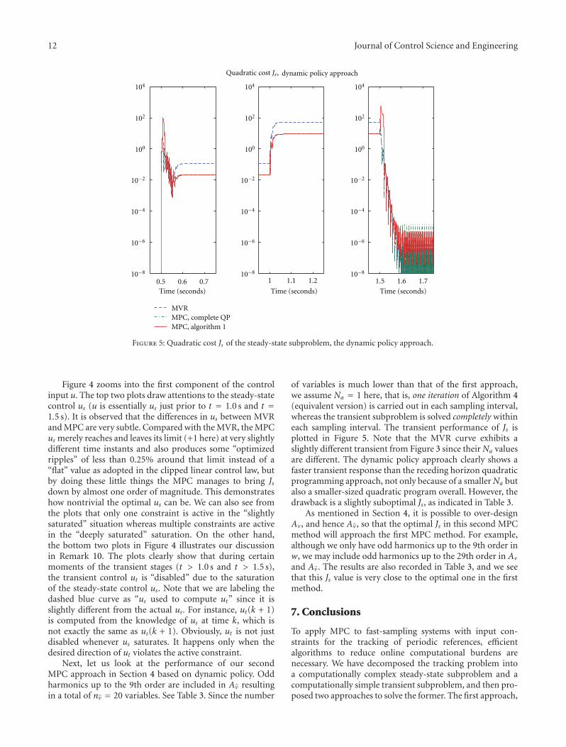
12 Journal of Control Science and Engineering
0.5 0.6 0.7Time (seconds)Time (seconds)Time (seconds)
1 1.1 1.210−8
10−6
10−4
10−2
100
102
104
10−8
10−6
10−4
10−2
100
102
104
10−8
10−6
10−4
10−2
100
102
104
1.5 1.6 1.7
MVRMPC, complete QPMPC, algorithm 1
Quadratic cost Js, dynamic policy approach
Figure 5: Quadratic cost Js of the steady-state subproblem, the dynamic policy approach.
Figure 4 zooms into the first component of the controlinput u. The top two plots draw attentions to the steady-statecontrol us (u is essentially us just prior to t = 1.0 s and t =1.5 s). It is observed that the differences in us between MVRand MPC are very subtle. Compared with the MVR, the MPCus merely reaches and leaves its limit (+1 here) at very slightlydifferent time instants and also produces some “optimizedripples” of less than 0.25% around that limit instead of a“flat” value as adopted in the clipped linear control law, butby doing these little things the MPC manages to bring Jsdown by almost one order of magnitude. This demonstrateshow nontrivial the optimal us can be. We can also see fromthe plots that only one constraint is active in the “slightlysaturated” situation whereas multiple constraints are activein the “deeply saturated” saturation. On the other hand,the bottom two plots in Figure 4 illustrates our discussionin Remark 10. The plots clearly show that during certainmoments of the transient stages (t > 1.0 s and t > 1.5 s),the transient control ut is “disabled” due to the saturationof the steady-state control us. Note that we are labeling thedashed blue curve as “us used to compute ut” since it isslightly different from the actual us. For instance, ut(k + 1)is computed from the knowledge of us at time k, which isnot exactly the same as us(k + 1). Obviously, ut is not justdisabled whenever us saturates. It happens only when thedesired direction of ut violates the active constraint.
Next, let us look at the performance of our secondMPC approach in Section 4 based on dynamic policy. Oddharmonics up to the 9th order are included in Av resultingin a total of nv = 20 variables. See Table 3. Since the number
of variables is much lower than that of the first approach,we assume Na = 1 here, that is, one iteration of Algorithm 4(equivalent version) is carried out in each sampling interval,whereas the transient subproblem is solved completely withineach sampling interval. The transient performance of Js isplotted in Figure 5. Note that the MVR curve exhibits aslightly different transient from Figure 3 since their Na valuesare different. The dynamic policy approach clearly shows afaster transient response than the receding horizon quadraticprogramming approach, not only because of a smaller Na butalso a smaller-sized quadratic program overall. However, thedrawback is a slightly suboptimal Js, as indicated in Table 3.
As mentioned in Section 4, it is possible to over-designAv, and hence Av, so that the optimal Js in this second MPCmethod will approach the first MPC method. For example,although we only have odd harmonics up to the 9th order inw, we may include odd harmonics up to the 29th order in Av
and Av. The results are also recorded in Table 3, and we seethat this Js value is very close to the optimal one in the firstmethod.
7. Conclusions
To apply MPC to fast-sampling systems with input con-straints for the tracking of periodic references, efficientalgorithms to reduce online computational burdens arenecessary. We have decomposed the tracking problem intoa computationally complex steady-state subproblem and acomputationally simple transient subproblem, and then pro-posed two approaches to solve the former. The first approach,

Journal of Control Science and Engineering 13
based on the concept of receding horizon quadratic pro-gramming, spreads the optimization over several samplingintervals, thus reducing the computational burdens at theprice of a slower transient response. The second approach,based on the idea of a dynamic policy on the control input,further reduces the online computations at the price ofa slightly suboptimal asymptotic performance. Despite thelimitations, these approaches make the application of MPCto fast-sampling systems possible. Their transient behavioursand steady-state optimality have been analyzed via computersimulations, which have also demonstrated that the steady-state subproblem and the transient subproblem can besolved in parallel with different sampling rates. Whenthe methods proposed in this paper are combined withmodern code optimizations, the applicability of MPC to theservomechanism of fast-sampling constrained systems willbe greatly enhanced.
Acknowledgment
This work is supported by HKU CRCG 201008159001.
References
[1] J. M. Maciejowski, Predictive Control with Constraints,Prentice-Hall, New Jersey, NY, USA, 2002.
[2] S. J. Qin and T. A. Badgwell, “A survey of industrial modelpredictive control technology,” Control Engineering Practice,vol. 11, no. 7, pp. 733–764, 2003.
[3] P. Whittle, Optimization Over Time, Wiley, New York, NY,USA, 1982.
[4] W. H. Kwon and S. Han, Receding Horizon Control, Springer,New York, NY, USA, 2005.
[5] A. Bemporad, M. Morari, V. Dua, and E. N. Pistikopoulos,“The explicit linear quadratic regulator for constrained sys-tems,” Automatica, vol. 38, no. 1, pp. 3–20, 2002.
[6] A. Bemporad, F. Borrelli, and M. Morari, “Min-max controlof constrained uncertain discrete-time linear systems,” IEEETransactions on Automatic Control, vol. 48, no. 9, pp. 1600–1606, 2003.
[7] A. Bemporad and C. Filippi, “Suboptimal explicit recedinghorizon control via approximate multiparametric quadraticprogramming,” Journal of Optimization Theory and Applica-tions, vol. 117, no. 1, pp. 9–38, 2003.
[8] Z. Wan and M. V. Kothare, “Robust output feedback modelpredictive control using off-line linear matrix inequalities,”Journal of Process Control, vol. 12, no. 7, pp. 763–774, 2002.
[9] Z. Wan and M. V. Kothare, “An efficient off-line formulation ofrobust model predictive control using linear matrix inequali-ties,” Automatica, vol. 39, no. 5, pp. 837–846, 2003.
[10] M. Akerblad and A. Hansson, “Efficient solution of secondorder cone program for model predictive control,” Interna-tional Journal of Control, vol. 77, no. 1, pp. 55–77, 2004.
[11] C. V. Rao, S. J. Wright, and J. B. Rawlings, “Application ofinterior-point methods to model predictive control,” Journal ofOptimization Theory and Applications, vol. 99, no. 3, pp. 723–757, 1998.
[12] J. Mattingley, Y. Wang, and S. Boyd, “Receding horizoncontrol: automatic generation of high-speed solvers,” IEEEControl Systems Magazine, vol. 31, no. 3, pp. 52–65, 2011.
[13] M. Cannon and B. Kouvaritakis, “Optimizing predictiondynamics for robust MPC,” IEEE Transactions on AutomaticControl, vol. 50, no. 11, pp. 1892–1897, 2005.
[14] A. Richards, K.-V. Ling, and J. Maciejowski, “Robust mul-tiplexed model predictive control,” in Proceedings of theEuropean Control Conference, Kos, Greece, July 2007.
[15] K. V. Ling, W. K. Ho, Y. Feng, and B. Wu, “Integral-square-error performance of multiplexed model predictive control,”IEEE Transactions on Industrial Informatics, vol. 7, no. 2, pp.196–203, 2011.
[16] D. Li and Y. Xi, “Aggregation based robust model predictivecontroller for systems with bounded disturbance,” in Pro-ceedings of the 7th World Congress on Intelligent Control andAutomation, (WCICA ’08), pp. 3374–3379, Chongqing, China,June 2008.
[17] D. Li and Y. Xi, “Aggregation based closed-loop MPC withguaranteed performance,” in Proceedings of the 48th IEEEConference on Decision and Control, (CDC/CCC ’09), pp.7400–7405, Shanghai, China, December 2009.
[18] J. B. Rawlings and K. R. Muske, “The stability of constrainedreceding horizon control,” IEEE Transactions on AutomaticControl, vol. 38, no. 10, pp. 1512–1516, 1993.
[19] K. H. Kwan, Y. C. Chu, and P. L. So, “Model-based H∞ controlof a unified power quality conditioner,” IEEE Transactions onIndustrial Electronics, vol. 56, no. 7, pp. 2493–2504, 2009.
[20] S. G. Nash and A. Sofer, Linear and Nonlinear Programming,McGraw-Hill, New York, NY, USA, 1996.
[21] J. Nocedal and S. J. Wright, Numerical Optimization, Springer,New York, NY, USA, 2nd edition, 2006.
[22] A. Gautam, Y.-C. Chu, and Y. C. Soh, “Robust MPC withoptimized controller dynamics for linear polytopic systemswith bounded additive disturbances,” in Proceedings of the 7thAsian Control Conference, (ASCC ’09), pp. 1322–1327, HongKong, China, August 2009.
[23] A. Gautam, Y.-C. Chu, and Y. C. Soh, “Optimized dynamicpolicy for receding horizon control of linear time-varyingsystems with bounded disturbances,” IEEE Transactions onAutomatic Control. In press.
[24] E. J. Davison, “The robust control of a servomechanismproblem for linear time-invariant multivariable systems,” IEEETransactions on Automatic Control, vol. 21, no. 1, pp. 25–34,1976.
[25] B. A. Francis and W. M. Wonham, “The internal modelprinciple of control theory,” Automatica, vol. 12, no. 5, pp.457–465, 1976.
[26] B. A. Francis, “The linear multivariable regulator problem,”SIAM Journal on Control Optimization, vol. 15, no. 3, pp. 486–505, 1977.

Hindawi Publishing CorporationJournal of Control Science and EngineeringVolume 2012, Article ID 630645, 6 pagesdoi:10.1155/2012/630645
Research Article
Pole Placement-Based NMPC of Hammerstein Systems andIts Application to Grade Transition Control of Polypropylene
He De-Feng and Yu Li
College of Information Engineering, Zhejiang University of Technology, Zhejiang, Hangzhou 310023, China
Correspondence should be addressed to He De-Feng, [email protected]
Received 1 July 2011; Accepted 11 September 2011
Academic Editor: Baocang Ding
Copyright © 2012 H. De-Feng and Y. Li. This is an open access article distributed under the Creative Commons AttributionLicense, which permits unrestricted use, distribution, and reproduction in any medium, provided the original work is properlycited.
This paper presents a new nonlinear model predictive control (MPC) algorithm for Hammerstein systems subject to constraints onthe state, input, and intermediate variable. Taking no account of constraints, a desired linear controller of the intermediate variableis obtained by applying pole placement to the linear subsystem. Then, actual control actions are determined in consideration ofconstraints by online solving a finite horizon optimal control problem, where only the first control is calculated and others areapproximated to reduce the computational demand. Moreover, the asymptotic stability can be guaranteed in certain condition.Finally, the simulation example of the grade transition control of industrial polypropylene plants is used to demonstrate theeffectiveness of the results proposed here.
1. Introduction
Hammerstein systems consist of the cascade connection ofa static (memoryless) nonlinear function followed from alinear dynamic system. Under certain assumptions (such asfading memory), the Hammerstein model could approxi-mately represent nonlinear dynamics of real systems andhas been successfully applied to many kinds of industrialprocesses such as pH neutralization [1], distillation [2], andpolymerization transition [3]. In recent years, constrainedcontrol of Hammerstein systems has become one of the mostneeded and yet very difficult tasks for the process industry.
Model predictive control (MPC) is an effective controlalgorithm for handling constrained control problems, andvarious MPC algorithms have been proposed for controlof Hammerstein systems with constraints [4–11]. Makinguse of the geometry structure of Hammerstein model,[4–9] developed two-step MPC schemes for Hammersteinsystems with input constraints, where the intermediatevariable was firstly obtained by linear MPC and then theactual control was calculated by solving nonlinear algebraicequations, desaturation, and so forth. Although two-stepMPC algorithms possess more light computational burden
than that where the nonlinearities were incorporated intooptimal control problems directly [10, 11], solving nonlin-ear algebraic equations will inevitably have error and therestricted control is generally different from the desired onefor constrained Hammerstein systems [6]. Therefore, theperformance and stability properties may be deteriorated inthe presence of constraints. Moreover, to the best of authors’knowledge, the conversional two-step MPC schemes usuallyhave limited ability to dealing with input constraints. So, [12]presented a new two-step MPC scheme for Hammersteinsystems with overall constraints, where the actual controllerwas determined by solving a finite horizon optimizationproblem that was described as tracking quadratic, optimaltrajectories of the intermediate variable. However, the onlinecomputational demand of optimization problem of thescheme is still an open question.
In this paper, we consider the problem of the grade tran-sition control of industrial polypropylene plants and proposean efficient NMPC scheme for Hammerstein systems withoverall constraints based on the pole placement method[13]. We firstly obtained desired trajectories of Hammersteinsystems by using pole placement to the linear subsystem andthen calculated actual control actions by solution of finite
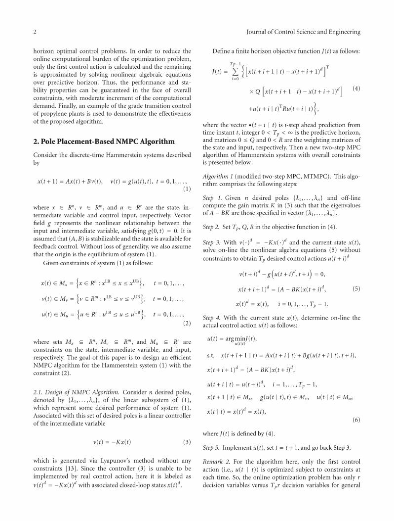
2 Journal of Control Science and Engineering
horizon optimal control problems. In order to reduce theonline computational burden of the optimization problem,only the first control action is calculated and the remainingis approximated by solving nonlinear algebraic equationsover predictive horizon. Thus, the performance and sta-bility properties can be guaranteed in the face of overallconstraints, with moderate increment of the computationaldemand. Finally, an example of the grade transition controlof propylene plants is used to demonstrate the effectivenessof the proposed algorithm.
2. Pole Placement-Based NMPC Algorithm
Consider the discrete-time Hammerstein systems describedby
x(t + 1) = Ax(t) + Bv(t), v(t) = g(u(t), t), t = 0, 1, . . . ,(1)
where x ∈ Rn, v ∈ Rm, and u ∈ Rr are the state, in-termediate variable and control input, respectively. Vectorfield g represents the nonlinear relationship between theinput and intermediate variable, satisfying g(0, t) = 0. It isassumed that (A,B) is stabilizable and the state is available forfeedback control. Without loss of generality, we also assumethat the origin is the equilibrium of system (1).
Given constraints of system (1) as follows:
x(t) ∈Mx ={x ∈ Rn : xLB ≤ x ≤ xUB
}, t = 0, 1, . . . ,
v(t) ∈Mv ={v ∈ Rm : vLB ≤ v ≤ vUB
}, t = 0, 1, . . . ,
u(t) ∈Mu ={u ∈ Rr : uLB ≤ u ≤ uUB
}, t = 0, 1, . . . ,
(2)
where sets Mx ⊆ Rn, Mv ⊆ Rm, and Mu ⊆ Rr areconstraints on the state, intermediate variable, and input,respectively. The goal of this paper is to design an efficientNMPC algorithm for the Hammerstein system (1) with theconstraint (2).
2.1. Design of NMPC Algorithm. Consider n desired poles,denoted by {λ1, . . . , λn}, of the linear subsystem of (1),which represent some desired performance of system (1).Associated with this set of desired poles is a linear controllerof the intermediate variable
v(t) = −Kx(t) (3)
which is generated via Lyapunov’s method without anyconstraints [13]. Since the controller (3) is unable to beimplemented by real control action, here it is labeled as
v(t)d = −Kx(t)d with associated closed-loop states x(t)d.
Define a finite horizon objective function J(t) as follows:
J(t) =Tp−1∑
i=0
{[x(t + i + 1 | t)− x(t + i + 1)d
]T
×Q[x(t + i + 1 | t)− x(t + i + 1)d
]
+u(t + i | t)TRu(t + i | t)}
,
(4)
where the vector •(t + i | t) is i-step ahead prediction fromtime instant t, integer 0 < Tp < ∞ is the predictive horizon,and matrices 0 ≤ Q and 0 < R are the weighting matrices ofthe state and input, respectively. Then a new two-step MPCalgorithm of Hammerstein systems with overall constraintsis presented below.
Algorithm 1 (modified two-step MPC, MTMPC). This algo-rithm comprises the following steps:
Step 1. Given n desired poles {λ1, . . . , λn} and off-linecompute the gain matrix K in (3) such that the eigenvaluesof A− BK are those specified in vector {λ1, . . . , λn}.
Step 2. Set Tp, Q, R in the objective function in (4).
Step 3. With v(·)d = −Kx(·)d and the current state x(t),solve on-line the nonlinear algebra equations (5) withoutconstraints to obtain Tp desired control actions u(t + i)d
v(t + i)d − g(u(t + i)d, t + i
)= 0,
x(t + i + 1)d = (A− BK)x(t + i)d,
x(t)d = x(t), i = 0, 1, . . . ,Tp − 1.
(5)
Step 4. With the current state x(t), determine on-line theactual control action u(t) as follows:
u(t) = arg minu(t|t)
J(t),
s.t. x(t + i + 1 | t) = Ax(t + i | t) + Bg(u(t + i | t), t + i),
x(t + i + 1)d = (A− BK)x(t + i)d,
u(t + i | t) = u(t + i)d, i = 1, . . . ,Tp − 1,
x(t + 1 | t) ∈Mx, g(u(t | t), t) ∈Mv, u(t | t) ∈Mu,
x(t | t) = x(t)d = x(t),(6)
where J(t) is defined by (4).
Step 5. Implement u(t), set t = t + 1, and go back Step 3.
Remark 2. For the algorithm here, only the first controlaction (i.e., u(t | t)) is optimized subject to constraints ateach time. So, the online optimization problem has only rdecision variables versus Tpr decision variables for general

Journal of Control Science and Engineering 3
nonlinear MPC, which results in a significant reduction ofthe online computational demand since the computationaldemand, in general, grows exponentially with the numberof decision variables [14]. Thus, the predictive horizonTp should be chosen reasonably large to ensure adequateperformance. On the other hand, since only the first controlis implemented in MPC scheme, it is expected that onlyenforcing constraints for the first prediction should giveexcellent results. In addition, the closed-loop performanceof MPC systems clearly depends on how n desired poles{λ1, . . . , λn} are arranged. The further work will focus on howto determine {λ1, . . . , λn} optimally.
It should be pointed out that the feasibility of optimiza-tion problem (6) may not be guaranteed theoretically withrespect to arbitrary constraints in (2). However, it is usuallyensured in practice via adjusting the intermediate variableconstraint. Next, we show that the closed-loop MPC system(1) is asymptotically stable, provided that the feasibility of(6) is hold.
2.2. Analysis of Stability. In terms of Algorithm MTMPC,the MPC law of constrained Hammerstein system (1), (2) isdefined as
u(t)MPC = u(t | t), t = 0, 1, . . . (7)
with the closed-loop system
x(t + 1) = Ax(t) + Bg(u(t)MPC, t
)
= (A− BK)x(t) + B[Kx(t) + g
(u(t)MPC, t
)].
(8)
Definition 3. Set M ⊆ Rn is called an attractive regionof system (8) if for all x(t) ∈ M, the system trajectoriesx(s; x(t)) → 0 when s → +∞ and satisfies
x(t) ∈M =⇒ x(t + 1)∈M, ∀u(t)MPC ∈Muv, t = 0, 1, . . . ,(9)
where subset Muv = {u ∈ Rr : g(u, ·) ∈Mv} ⊆Mu.
Let a set of points {λ1, . . . , λn} be the desired poles of thelinear subsystem x(t+ 1) = (A−BK)x(t). Then from inverseLyapunov’s theorem [13], there is systematic matrices P > 0and Q > 0 such that
(A− BK)TP(A− BK)− P < −Q. (10)
In following, we present the result on our proposed algo-rithm.
Theorem 4. Consider the system (1), (2), there exists anonempty region M such that the closed-loop system (8) is as-ymptotically stable if the inequality (11) is satisfied
V(x(t + 1)) ≤ V(x(t + 1)d
), ∀x(t) ∈M, t = 0, 1, . . . ,
(11)
where function V(x) = xTPx and x(t + 1)d = (A − BK)x(t)d
with x(t)d = x(t). Moreover, the set M is an attractive regionof system (8).
Proof. Consider the system (1), (2), define a level set M offunction V(x) as
M = {x ∈ Rn : V(x) ≤ c, c > 0} ⊆Mx (12)
such that u(t)MPC ∈ Muv, for all x(t) ∈ M, t = 0, 1, . . .. Notethat the set M is always nonempty since the constraint in (2)includes the origin as the internal point.
Let function V(x) be a Lyapunov function candidate ofsystem (8). Then, for any x(t) ∈M, we have
V(x(t + 1))−V(x(t))
= x(t + 1)TPx(t + 1)− x(t)TPx(t)
= x(t)T(A− BK)TP(A− BK)x(t)T
− x(t)TPx(t) + 2x(t)T(A− BK)TPBΔ + ΔTBTPBΔ
= x(t)T[
(A− BK)TP(A− BK)− P]x(t)
+ 2x(t)T(A− BK)TPBΔ + ΔTBTPBΔ,(13)
where Δ = g(u(t)MPC, t)+Kx(t) = g(u(t)MPC, t)−v(t)d. Sub-stituting (10) into (13) yields
V(x(t + 1))−V(x(t))
= −x(t)TQx(t) + 2[(A− BK)x(t)]TPBΔ + ΔTBTPBΔ
= −x(t)TQx(t) + 2x(t)TATPBΔ
+ 2(g − Δ
)TBTPBΔ + ΔTBTPBΔ
= −x(t)TQx(t) + 2x(t + 1)TPBΔ− ΔTBTPBΔ
= −x(t)TQx(t)− x(t + 1)dTPx(t + 1)d
+ x(t + 1)TPx(t + 1)
= −x(t)TQx(t)−V(x(t + 1)d
)+ V(x(t + 1)).
(14)
From the inequality (11), it is straight forward to obtain that
V(x(t + 1))−V(x(t)) ≤ −x(t)TQx(t), ∀x(t) ∈M. (15)
Hence, function V(x) is a Lyapunov function of system(8), and the system is asymptotically stable in region M.Furthermore, from the definition of attractive regions and setM in (12), we derive that M is an attractive region of system(8).
This establishes the theorem.

4 Journal of Control Science and Engineering
Remark 5. From the proof of the above theorem, we knowthat the stability property of closed-loop system (8) is guar-anteed by the linear controller of the intermediate variable,provided that the feasibility of optimization problem (6)and condition (11) holds. This suggests that the stabilityand optimality can be separated to some extent. Therefore,the design parameter of the objective function in (4) canbe tuned freely to achieve more satisfactory performance,regardless the stability of the closed-loop system. In addition,it is pointed out that the attractive region M obtained here ismerely a theoretical concept and the computation of M is notan easy task.
Remark 6. Instead of conventional two-step MPC algo-rithms, where the actual control was determined by solvingnonlinear algebraic equations based on desired controllersof the intermediate variable resulted from linear MPC,actual control actions here are derived by solving a finitehorizon optimal control problem (i.e., nonlinear MPC),which is defined as tracking the desired state trajectoriesdriven by pole placement state feedback controller. Thus,overall constraints of Hammerstein systems are taken intoaccount when designing the predictive controller, and thenperformance and stability properties are guaranteed. Mean-while, the ability to handling constraints is enhanced in thealgorithm proposed here. Note that the linear controller ofintermediate variables in (3) can be any one that stabilizesthe linear subsystems of Hammerstein models with certaindesired performance.
3. Simulation Example
Taking an example of polypropylene (PP) grade transitioncontrol, we illustrate the effectiveness of the proposedalgorithm.
In propylene polymerization industry, melt index (MI,g/10 min) is usually used to identify grade indices of PPhomopolymer and both of MI and concentration of ethylene(Et, %) in PP denote grade indices of total phase PP [12, 15–18]. This implies that the nature of grade transition processis to operate the response of the variables MI and Et inpolymer. Then according to the propylene polymerizationmechanism, we have the following mathematical modelwhich formulates the dynamics of the grade transition inpolypropylene process [12]:
⎡⎣x1
x2
⎤⎦ =
⎡⎢⎢⎣−1τ
0
0 −1τ
⎤⎥⎥⎦
⎡⎣x1
x2
⎤⎦ +
⎡⎢⎢⎣
1τ
0
01τ
⎤⎥⎥⎦
⎡⎣g1(u, t)
g2(u, t)
⎤⎦,
⎡⎣g1(u, t)
g2(u, t)
⎤⎦ =
⎡⎢⎢⎣k1 +
k2
u1+ k3 log(k4 + k5u2 + k6u3)
k7u2 + 1k8/u3 + k9u3 + k10
⎤⎥⎥⎦,
y(t) =⎡⎣1 0
0 1
⎤⎦x(t), t ≥ 0,
(16)
0 10 20 30 40 50 60 70 80 90 1000
10
20
30
40
50
Times (0.5 h)
MI
(g/1
0m
in)
Grade A
Grade B
Grade C
(a) Melt index
0 10 20 30 40 50 60 70 80 90 100
3
2
1
0
Times (0.5 h)
Grade A Grade B
Grade C
Et
(%)
(b) Concentration of ethylene in polypropylene
Figure 1: MI and Et output trajectories of grade transitionprocesses. (Solid line is the set-point, dotted line the instantaneous,and dashed line the cumulative).
where states x1 and x2 are the cumulative MI (MIc, g/10 min)and Et (Etc, %) of PP, respectively; intermediate variablesg1 and g2 denote the instantaneous MI (MIi, g/10 min)and Et (Eti, %) of PP, respectively; input, u1, u2, u3
denote the reaction temperature T(K), concentration ratioof hydrogen to propylene CH2/Cm (%), and concentrationratio of ethylene to propylene Cm2/Cm (%), respectively, andparameter τ is the average polymer residence time (τ = 2 h).The parameters of model ki (i = 1, . . . , 10) can be identifiedon-line by industrial data [15].
The grade transition sequence considered here is A→B→C, where grades A and B are PP homopolymer and Cis total phase PP. It should be pointed out that the feedflow rate of ethylene is always zero (i.e., [Cm2/Cm] = 0)in production of PP homopolymer grades A and B. Thegrade transition process is defined by the set-point of statesand input/output constraints as shown in Table 1, wheresuperscripts c, i, and Δ denote accumulation, instantaneousvalue, and increment constraints, respectively. Each gradetransition is optimized over 10 h horizon with a samplinginterval of 0.5 h.
In the simulation running, the closed-loop desired polesof system (16) are placed at {λ1, λ2} = {0.72, 0.60}, and thecorresponding state-feedback matrix K in (3) is computedby K = [0.12, 0; 0, 0.6]. Moreover, the parameters in theobjective function (4) are chosen as penalty on the states,Q = qI2, with q = 1, penalty on the inputs, R = I3 anda horizon length of Tp = 20. Assume that grade transitionA→B takes place at the tenth hour and B→C at the thirtiethhour. Then some curves of the grade transition process beingcontrolled by NMPC law are shown in Figures 1 and 2, wherethe solid line in Figure 1 is the set-point, the dotted line theinstantaneous, and the dashed line the cumulative.

Journal of Control Science and Engineering 5
Table 1: Grade indices and transition constraints.
Grade MI (g/10 min) Et (%) T (K) CH2 (%) Cm2/Cm (%)
A 2.7 — 343.15 0.050 —
B 39.0 — 343.15 0.330 —
C 10.0 2.4 343.15 0.236 1.99
A→B[2.4, 42.0]c — [341.15, 345.15] [0.02, 0.35] —
[2.0, 45.0]i — — [−0.1, 0.10]Δ —
B→C[8.0, 42.0]c [0.0, 2.5]c [341.15, 345.15] [0.20, 0.35] [0.00, 2.50]
[6.0, 45.0]i [0.0, 2.6]i — [−0.1, 0.10]Δ [−0.1, 0.10]Δ
0 10 20 30 40 50 60 70 80 90 100
Times (0.5 h)
345
344
343
342
Grade A Grade B Grade C
T(K
)
(a) Reaction temperature
0 10 20 30 40 50 60 70 80 90 100
Times (0.5 h)
0.4
0.2
0
Grade A
Grade BGrade C
CH
2/C
m(%
)
(b) Concentration ratio of hydrogen to propylene
0 10 20 30 40 50 60 70 80 90 100
Times (0.5 h)
3
2
1
0Grade A Grade B
Grade C
Cm
2/C
m(%
)
(c) Concentration ratio of ethylene to propylene
Figure 2: Input profiles of grade transition processes.
In order to calculate the quantity of off-specificationpolymer in grade transition process, we employ the criterionwhere on-specification polymer is defined as the polymerwith MIc and Etc within a ±5% deviation of desiredspecification in Table 1. All other polymers beyond thecriterion are categorized as off-specification production.Similarly, the transition time is defined as the time intervalwhen the cumulative properties of polymer are out of thespecification range ±5% of the previous grade and lastinguntil the cumulative properties enter and stay within thespecification range ±5% of the new target grade. Therefore,the time of grade A→B transition is 8.5 hours and thetime of grade B→C transition is 6.5 hours. Compare to thetime of 10 hours in actual grade transition operation, thisdecreases the quantity of off-specification polymer in gradetransition process and then increases the productive timeof on-specification polymer. Also, Figure 2(a) suggests thatthere is no change in reaction temperature during the gradetransition processes, which is desired in actual operation.Finally, it can be seen that the control laws, intermediate
variables, and the states in the grade transition operation donot violate the constraints in Table 1.
4. Conclusion
Together with the pole placement method, the paper pre-sented an efficient MPC algorithm for control of Hammer-stein systems subject to constraints on states, inputs, andintermediate variables. Applying pole placement to the linearsubsystem of Hammerstein models yielded linear controllersof the intermediate variable and then the actual controlaction was determined by online solving an optimizationproblem. The size of the online optimization problemdepended only on the number of inputs, not on thepredictive horizon, which greatly reduced the computationaldemand of the algorithm. With condition of feasibility ofthe optimization problem, the asymptotical stability of theclosed-loop system with constraints was guaranteed and theresults on simulation example of grade transition control ofpolypropylene plants showed the effectiveness of the resultsobtained here.
Acknowledgments
This work is supported by the National Natural ScienceFoundation of China under Grant no. 60904040, SpecializedResearch Fund for Doctoral Program of Higher Education ofChina under Grant no. 20093317120002 and Natural ScienceFoundation of Zhejiang Province under Grant no. Y1100911.Finally, the authors are grateful to the reviews’ constructivecomments. This paper includes revised and extended text ofthe first author’s presentation at the 29th CCC, July 27, 2010,Beijiang, China.
References
[1] Z. Hasiewicz, “Hammerstein system identification by theHaar multiresolution approximation,” International Journal ofAdaptive Control and Signal Processing, vol. 49, pp. 691–717,1999.
[2] N. Bhandari and D. Rollins, “Continuous-time Hammersteinnonlinear modeling applied to distillation,” AIChE Journal,vol. 50, no. 2, pp. 530–533, 2004.
[3] D. F. He, L. Yu, and M. S. Xue, “On operation guidancefor grade transition in propylene polymerization plants,” inProceedings of the 19th Chinese Process Control Conference, pp.339–342, Beijiang, China, 2008, (Chinese).

6 Journal of Control Science and Engineering
[4] Q. M. Zhu, K. Warwick, and J. L. Douce, “Adaptive generalpredictive controller for nonlinear systems,” IEE ProceedingsD, vol. 138, no. 1, pp. 33–40, 1991.
[5] K. P. Fruzzetti, A. Palazoglu, and K. A. McDonald, “Nonlinearmodel predictive control using Hammerstein models,” Journalof Process Control, vol. 7, no. 1, pp. 31–41, 1997.
[6] B. C. Ding, Y. G. Xi, and S. Y. Li, “Stability analysis onpredictive control of discrete-time systems with input non-linearity,” Acta Automatica Sinica, vol. 29, no. 6, pp. 827–834,2003.
[7] B. C. Ding, Y. G. Xi, and S. Y. Li, “On the stability ofoutput feedback predictive control for systems with inputnonlinearity,” Asian Journal of Control, vol. 6, no. 3, pp. 388–397, 2004.
[8] B. Ding and Y. Xi, “A two-step predictive control design forinput saturated Hammerstein systems,” International Journalof Robust and Nonlinear Control, vol. 16, no. 7, pp. 353–367,2006.
[9] H. T. Zhang, H. X. Li, and G. Chen, “Dual-mode predictivecontrol algorithm for constrained Hammerstein systems,”International Journal of Control, vol. 81, no. 10, pp. 1609–1625,2008.
[10] H. H. J. Bloemen and T. J. J. van den Boom, “Model-basedpredictive control for Hammerstein systems,” in Proceedings ofthe 39th IEEE Conference on Decision and Control, vol. 5, pp.4963–4968, Sydney, Australia, 2000.
[11] H. H. J. Bloemen, T. J. J. van den Boom, and H. B. Verbruggen,“Model-based predictive control for Hammerstein-Wienersystems,” International Journal of Control, vol. 74, pp. 482–495,2005.
[12] D. F. He and L. Yu, “Nonlinear predictive control of con-strained Hammerstein systems and its research on simulationof polypropylene grade transition,” Acta Automatica Sinica,vol. 35, no. 12, pp. 1558–1563, 2009 (Chinese).
[13] C. T. Chen, Linear system Theory and Design, Oxford Univer-sity Press, New York, NY, USA, 3rd edition, 1999.
[14] A. Zheng, “A computationally efficient nonlinear MPC algo-rithm,” in Proceedings of the American Control Conference, pp.1623–1627, Albuquerque, NM, USA, June 1997.
[15] J. R. Richards and J. P. Congalidis, “Measurement andcontrol of polymerization reactors,” Computers and ChemicalEngineering, vol. 30, no. 10–12, pp. 1447–1463, 2006.
[16] H. S. Yi, J. H. Kim, C. Han, J. Lee, and S. S. Na, “Plantwideoptimal grade transition for an industrial high-densitypolyethylene plant,” Industrial and Engineering ChemistryResearch, vol. 42, no. 1, pp. 91–98, 2003.
[17] Y. Wang, H. Seki, S. Ohyama, K. Akamatsu, M. Ogawa, andM. Ohshima, “Optimal grade transition control for polymer-ization reactors,” Computers and Chemical Engineering, vol. 24,no. 2–7, pp. 1555–1561, 2000.
[18] T. Kreft and W. F. Reed, “Predictive control of average com-position and molecular weight distributions in semibatch freeradical copolymerization reactions,” Macromolecules, vol. 42,no. 15, pp. 5558–5565, 2009.