journal of civil engineering and architecture09-5
TRANSCRIPT


David Publishing Company
www.davidpublishing.com
PublishingDavid
Journal of Civil Engineering
and Architecture
Volume 3, Number 5, May 2009 (Serial Number 18)

Publication Information: Journal of Civil Engineering and Architecture (ISSN1934-7359) is published monthly in hard copy and online by David Publishing Company located at 1840 Industrial Drive, Suite 160, Libertyville, Illinois 60048, USA. Aims and Scope: Journal of Civil Engineering and Architecture, a monthly professional academic journal, covers all sorts of researches on structure engineering, geotechnical engineering, underground engineering, engineering management, etc. as well as other issues. Editors: Markus, C., Linda, Z., Engles, Z., Barbie, W., Tina Z., Lily L., Jim Q., Hiller H., Jane C., Betty Z., Gloria G., Stella H., Alina Y., Ben Y., Hubert H., Ryan H.. Manuscripts and correspondence are invited for publication. You can submit your papers via Web Submission, or E-mail to [email protected] or [email protected]. Submission guidelines and Web Submission system are available at http://www.davidpublishing.com. Editorial Office: 1840 Industrial Drive, Suite 160 Libertyville, Illinois 60048 Tel: 1-847-281-9826 Fax: 1-847-281-9855 E-mail: [email protected]; [email protected] Copyright©2009 by David Publishing Company and individual contributors. All rights reserved. David Publishing Company holds the exclusive copyright of all the contents of this journal. In accordance with the international convention, no part of this journal may be reproduced or transmitted by any media or publishing organs (including various websites) without the written permission of the copyright holder. Otherwise, any conduct would be considered as the violation of the copyright. The contents of this journal are available for any citation. However, all the citations should be clearly indicated with the title of this journal, serial number and the name of the author. Abstracted / Indexed in: Database of EBSCO, Massachusetts, USA Chinese Database of CEPS, Airiti Inc. & OCLC Cambridge Science Abstracts (CSA) Ulrich’s Periodicals Directory Subscription Information: Price: $96 (12 issues) David Publishing Company 1840 Industrial Drive, Suite 160, Libertyville, Illinois 60048 Tel: 1-847-281-9826. Fax: 1-847-281-9855 E-mail: [email protected]
David Publishing Company
w ww.davidpublishing.com
Pub lishingDavid

Journal of Civil Engineering and Architecture
Volume 3, Number 5, May 2009 (Serial Number 18)
Contents Model Simulation and Calculation
Seismic analysis of a long-span continuous steel truss-arch bridge across the Yangtze River 1 XIA Chao-yi, LEI Jun-qing, XIA He, PI Yong-lin
3D building modeling: A critical investigation practice to learning, analyzing and deconstruting architecture 9
Andrea Cammarata
Experimental Study
Underground water biological field’s variation and geoenvironmental safety in city 16 YI Nian-ping, ZHANG Xin-gui, WANG Yang, Huang Jun-peng
A statistically refined Bouc-Wen model for the identification of structures under tri-directional seismic excitations 22
LIN Jeng-wen
Tall building configuration effects on their response to earthquake loading 30 Mohammed S. Al-Ansari
Experimental analysis of Tuned Liquid Damper (TLD) for high raised structures 40 S. Arash Sohrabi, Samad Dehghan
The influence of Fe extracting as a filler of fiber concrete performance 46 Nawir Rasidi
Architecture Environment
The leasing operation of research of the office building market in China 53 QIU Guo-lin
Design and construction of high and large span cast-in-place reinforced concrete cantilever flowering frame beam 58
WANG Rui, ZHEN Liang, WAN Chao, WU Jing, SHEN Yan-jun


May 2009, Volume 3, No.5 (Serial No.18) Journal of Civil Engineering and Architecture, ISSN 1934-7359, USA
1
Seismic analysis of a long-span continuous steel truss-arch
bridge across the Yangtze River*
XIA Chao-yi1, LEI Jun-qing1, XIA He1, PI Yong-lin2 (1. School of Civil Engineering, Beijing Jiaotong University, Beijing 100044, China;
2. School of Civil & Environmental Engineering, The University of New South Wales, Sydney 2052, Australia)
Abstract: In this paper, an FEM (Finite Element Method) model is established for the main span of the bridge, with the main box arch and suspender members modeled by beam elements, truss members by truss elements, and the orthotropic steel deck by plate elements. The natural frequencies and mode shapes are acquired by the eigen-parameter analysis. By input of a typical earthquake excitation to the bridge system, the dynamic responses of the bridge, including the displacement and accelerations of the main joints of the structure, and the seismic forces and stresses of the key members, are calculated by the structural analysis program, based on which the main laws of the seismic responses of the bridge are summarized, and the safety of the structure is evaluated. Key words: FEM; main span of the bridge; natural frequencies; the dynamic responses
1. Introduction
Arch bridges, owing to its high stiffness and nice appearance, are used as one of the important types of railway bridge. The Nanjing Dashengguan Bridge is an important part and one of the key engineering works of the Beijing-Shanghai high-speed railway. The construction of bridge was started in the beginning of 2006. The view of the bridge is shown in Fig. 1.
It is a long span railway bridge across the Yangtze River, designed with many new materials, structures and construction technologies, using 80,000 t steel in total. The major part of the bridge is composed of 108
* Acknowledgments: This study is sponsored by the Natural Science Foundation of China (No. 90715008) and the Flander (Belgium)-China Bilateral Project (No. BIL07/07).
XIA Chao-yi, Ph.D.; research field: bridge engineering. Corresponding author: XIA He, professor; research fields:
bridge vibration and structure driving force reliability reason with application. E-mail: [email protected].
+192+336+336+192+108 m six-span continuous truss-arch structures, and side spans of 2×84 m continuous trusses at each side of the major part of the bridge. The structure has a feature of long span, long suspender low damping[1]. The dynamic behavior of this bridge under earthquake excitations is one of the main problems to be solved in the design of the structure.
(a)
(b)
Fig. 1 The Nanjing Dashengguan Yangtze River Bridge
Earthquake is one of the most serious natural disasters in the world. The dynamic behaviours of bridges under earthquakes have been studied by researches in China and abroad[2]
T. Tseng and Penzien established mathematical models Ton Tlong, curved (or straight), multiple-span, reinforced concrete highway bridges and performed three-dimensional
Seismic analysis of a long-span continuous steel truss-arch bridge across the Yangtze River
2
non-linear seismic analysis[3]; Abdel-Ghaffar, et al proposed a seismic performance evaluation method for suspension bridges[4]; Dumanoglu, et al analyzed the stochastic response of suspension bridges to earthquake excitations, and estimated the spatial dynamic responses of the Fatih Sultan Mehmet (second Bosporus) suspension bridge under earthquake excitation with different speeds of wave propagation, respectively[5-6]; Saiidi, et al calculated the seismic performance of the Madrone Bridge during the 1989 Loma Prieta Earthquake[7]; ZHU and LAO compared the selection methods of input earthquake waves for seismic analysis of bridges[8]; Lupoi, et al investigated seismic behaviours of bridges accounting for spatial variability of ground motion[9]; T Ribeiro, et al studied the dynamic responses of the Alcácer do Sal Railway Bridge, 8 span simply supported steel bowstring arch bridge, on the Southern Line of the Portuguese Railways[10]; Kim and Kawatani proposed a modal analysis model to study the three-dimensional responses of steel monorail bridges under moderate earthquake excitations[11]; CAO and ZHONG performed a seismic analysis on a long-span cable-stayed bridge across the Yangtze River[12].
For arch bridges have distinct seismic features, GUO and YANG established a seismic analysis model to calculate the dynamic responses of a steel tubular concrete arch bridge[13]; Usami, et al proposed a three-dimensional analysis model to investigate the seismic performance evaluation of steel arch bridges to strong ground motions from major earthquakes, by using the modified ground motions based on the records from the 1995 Hyogoken-Nanbu earthquake[14]; LI and GE studied the seismic responses of a 5-span half-through CFST arch bridge[15], XU Ji studied the seismic performance of a large-span RC arch bridge[16]; Galvín and Domínguez performed dynamic analysis on a cable-stayed steel arch bridge[17], and ZHAO and LI performed dynamic analysis on a continuous rigid-frame arch bridge[18].
In this paper, an FEM model is established for the main span of the bridge, with the main box arch and suspender members modeled by beam elements, truss members by truss elements, and the orthotropic steel deck by plate elements. The natural frequencies and mode shapes are acquired by the eigen-parameter analysis. By input of the Tianjin earthquake acceleration waves to the bridge system, the dynamic responses of the bridge, including the displacement and accelerations of the main joints of the structure, and the seismic forces and stresses of the key members, are calculated by the structural analysis program, based on which the main properties of the seismic responses of the bridge are summarized, and the safety of the structure is evaluated.
2. Bridge’s analysis model
2.1 Introduce to the bridge The Nanjing Dashengguan Yangtze River Bridge
under construction is a long span rail-cum-road bridge across the Yangtze River, which is designed with many new materials, structures and construction technologies.
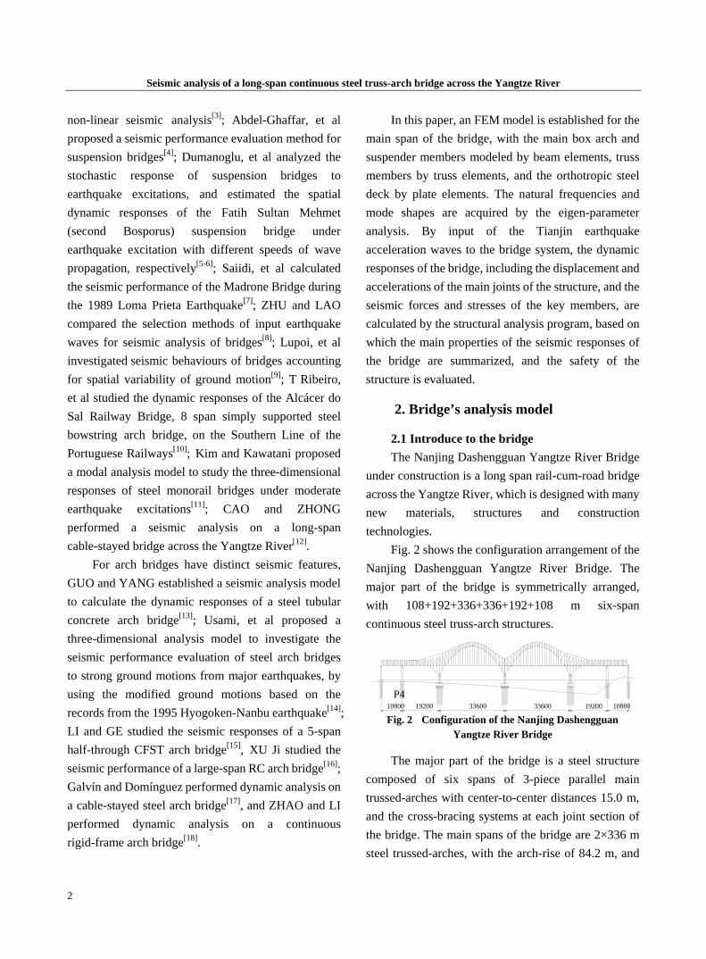
Fig. 2 shows the configuration arrangement of the Nanjing Dashengguan Yangtze River Bridge. The major part of the bridge is symmetrically arranged, with 108+192+336+336+192+108 m six-span continuous steel truss-arch structures.
10800 19200 33600 33600 19200 10800 Fig. 2 Configuration of the Nanjing Dashengguan
Yangtze River Bridge
The major part of the bridge is a steel structure composed of six spans of 3-piece parallel main trussed-arches with center-to-center distances 15.0 m, and the cross-bracing systems at each joint section of the bridge. The main spans of the bridge are 2×336 m steel trussed-arches, with the arch-rise of 84.2 m, and
P4

Seismic analysis of a long-span continuous steel truss-arch bridge across the Yangtze River
3
thus a rise-to-span ratio of 1:4. The height of arch rib is 12 m at the arch crowns and 56 m at the arch springings. The total height of the arch is 96.2 m from the springing to the crown. Next to the main arches are N-shaped flat chord trusses which are 16 m in height, with the panel length of 12 m for most panels and 15 m for the four panels close to each arch springing. The flat chord truss and the arched truss are connected with variable height panels. The bridge deck for railways is 28 m above the springing level.
Fig. 3 is showing the cross section arrangement of the main truss part of the bridge. To meet the requirement of running safety and stability of the trains, the deck of the bridge is designed as monolithic orthotropic steel plate stiffened with longitudinal and transverse ribs and connected with the lower chords of the main truss, forming a plate-truss composite structure, so as that the deck plate jointly participates in the internal force bearing of the truss members (see Fig. 4). The deck is 41.6 m in width, which carries six tracks, including two tracks (G1, G2) for high-speed trains of 300 km/h, two tracks (P1, P2) for conventional trains of 120 km/h (freight) and/or 200 km/h (passenger), and two tracks (U1, U2) for urban subway trains of 80 km/h. The two subway tracks are 5.8 m in width, located on the cantilevered decks projected from the outer sides of the main truss, the central line of the tracks are 3.25 m from the center of truss chords.
1500
200 200260
1500
4160
325 255
U2
200 200300 200
325255
200
U1 P2P1G2G1
Fig. 3 Cross section arrangement of the bridge
2.2 Bridge modeling The bridge is modeled by the structural analysis
software ANSYS. All members in the main truss, including the three peaces of arch ribs, upper and lower
chords, hangers, vertical and diagonal web members, top and bottom longitudinal bracing members, and cross-bracing members, are regarded as spatial beam elements in the FEM model.
The bridge deck system is modeled with “beam-grid” method, where the orthotropic plate and the stiffening ribs are simplified as six longitudinal beams, with each supporting a railway track, and as main and secondary cross beams in each panel of the main span. The equivalent section properties of a beam are calculated with the section properties of the actual structure within the area represented by the beam. The weights of the steel deck and the secondary loads are distributed to the longitudinal beam.
The main spans are supported by three huge pot neoprene bearings on each pier-cap of 12.5 m × 40.5 m × 3.0 m in dimension, and the maximum reaction capacity of each bearing is up to 170,000 kN.
The main piers of the bridge are designed with a round-end hollow cross section, which has the plane size of 12.0 m × 40.0 m, with the round wall thickness of 1.5 m, and a central partition wall 4.0 m. The platforms are 34 m × 76 m × 6 m in dimension, which are supported by 46 bored piles with the diameter of 2.5 m (see Fig. 4).
Fig. 4 Foundation model of the bridge pier
The piers are modeled with spatial beam elements, and the platforms by block elements. The connections

Seismic analysis of a long-span continuous steel truss-arch bridge across the Yangtze River
4
between the pier cap and the main structure are treated as master-and-slave freedoms.
The stiffness of the pile foundations and the surrounding soils are simplified as equivalent base springs, with their stiffness added onto the corresponding platform nodes. The spring stiffnesses
of the equivalent base springs are listed in Table 1, where KX, KY and KZ are the translation stiffnesses in longitudinal, transverse and vertical directions, and KRX, KRY and KRZ are rotational stiffnesses corresponding to the longitudinal, transverse and vertical axes of the bridge, respectively.
Table 1 Foundation stiffness of the bridge piers
Pier KX /GN KY /GN KZ /GN KRX /GN·m-1 KRY /GN·m-1 KRZ /GN·m-1 P4 1.077 1.047 62.10 9121 2209 224.3 P5 0.9950 0.9700 67.09 12870 2384 257.8 P6 3.524 3.524 162.9 58410 15470 1745 P7 1.931 1.931 157.5 56350 56350 1007 P8 0.4287 0.4287 127.6 45500 11870 285.9 P9 0.3447 0.3384 58.56 11200 2049 105.1
P10 6.758 5.710 48.12 6160 1810 822.7
Fig. 5 FEM model of the bridge
Totally, there are 3771 nodes and 8507 spatial beam elements in the bridge model. The FEM model of the Nanjing Yangtze River Bridge is shown in Fig. 5.
The total weight of the bridge structure is about 110,000 t, in which the self-weight of the main
structure is 554 kN/m, and the secondary load including the track and other railway facilities is taken as 388 kN/m in the modal analysis.
2.3 Modal analysis of bridge The natural vibration properties of the bridge are
analyzed by the general structural analysis software ANSYS. There are 80 orders of natural frequencies and mode shapes for the bridge are obtained. The descriptions for the first 10 modes are given in Table 2, and the first 6 mode shapes of the bridge are shown in Fig. 6.
Table 2 Modal properties of the bridge
No. Freq. /Hz Mode description 1 0.3425 1st vertical anti-symmetry of arch. 2 0.3781 1st lateral anti-symmetry with arch and deck in phase. 3 0.4100 2nd lateral symmetry with arch and deck in phase. 4 0.5968 2nd vertical symmetry of arch. 5 0.6290 3rd vertical anti-symmetry of arch. 6 0.6641 3rd lateral symmetry with arch and deck out of phase. 7 0.6717 4th lateral anti-symmetry with arch and deck out of phase. 8 0.7387 4th vertical symmetry of arch. 9 0.8048 5th lateral symmetry with arch and deck in phase. 10 0.8281 6th lateral anti-symmetry with arch and deck in phase.

Seismic analysis of a long-span continuous steel truss-arch bridge across the Yangtze River
5
(a) The first vertical mode (front view) (b) The first lateral mode (plan view)
(c) The second vertical mode (front view) (d) The second lateral mode (plan view)
(e) The third vertical mode (front view) (f) The third lateral mode (plan view)
Fig. 6 Natural vibration modes of the bridge
As is seen in Table 1 and Fig. 5, the first mode of the six-span continuous steel truss-arch bridge is a vertical movement in anti-symmetry, with the frequency 0.3425 Hz. The second mode is a lateral movement in anti-symmetry with arch and girder in phase and frequency 0.3781 Hz.
One can also see that the natural frequencies of the bridge are rather low, with its tenth frequency only 0.8281 Hz. This result indicates that the six-span continuous steel truss-arch bridge is rather flexible.
3. Seismic analysis of bridge
3.1 Earthquake excitation to the bridge The earthquake acceleration record at Tianjin
during the Tangshan Earthquake in China is taken as the input to the bridge, to analyze the seismic responses of the structure.
The earthquake took place at 21:53, on November 25, 1976, with its record length 19.12 sec, richter magnitude 6.9, epicentral distance 65 km, frequency component 0.30-35.00 Hz. The peak accelerations in x, y and z directions are 104.1804 gal, 145.8047 gal and 73.1401 gal, respectively. Fig. 7 is showing the original accelerometers of the Tianjin Earthquake record.
-120
-70
-20
30
80
0 2 4 6 8 10 12 14 16 18 20
Time /s
Acc
eler
atio
n /g
al
(a) Horizontal acceleration (direction x)
-160-120
-80-40
04080
120160
0 2 4 6 8 10 12 14 16 18 20
Time /s
Acc
eler
atio
n /g
al
(b) Horizontal acceleration (direction y)
-80-60-40-20
020406080
0 2 4 6 8 10 12 14 16 18 20
Time /s
Acc
eler
atio
n /g
al
(c) Vertical acceleration
Fig. 7 Accelerations of the Tianjin earthquake record
According to the Chinese Aseismic Design Code for Railway Bridges, the earthquake intensity for the
Seismic analysis of a long-span continuous steel truss-arch bridge across the Yangtze River
6
area where the Nanjing Dashengguan Yangtze River Bridge locates is 7 degree. Thus the peak accelerations in three directions of the Tianjin earthquake record were normalized to be 0.125g in horizontal direction and 0.0625g in vertical direction.
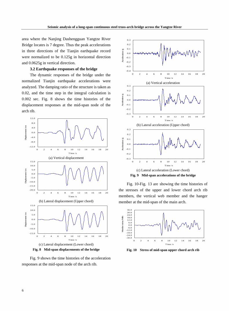
3.2 Earthquake responses of the bridge The dynamic responses of the bridge under the
normalized Tianjin earthquake accelerations were analyzed. The damping ratio of the structure is taken as 0.02, and the time step in the integral calculation is 0.002 sec. Fig. 8 shows the time histories of the displacement responses at the mid-span node of the arch rib.
-12.0
-8.0
-4.0
0.0
4.0
8.0
12.0
0 2 4 6 8 10 12 14 16 18 20
Time /s
Disp
lace
men
t /cm
(a) Vertical displacement
-20.0
-15.0
-10.0
-5.0
0.0
5.0
10.0
15.0
0 2 4 6 8 10 12 14 16 18 20
Time /s
Disp
lace
men
t /cm
(b) Lateral displacement (Upper chord)
-15.0
-10.0
-5.0
0.0
5.0
10.0
15.0
0 2 4 6 8 10 12 14 16 18 20
Time /s
Disp
lace
men
t /cm
(c) Lateral displacement (Lower chord)
Fig. 8 Mid-span displacements of the bridge
Fig. 9 shows the time histories of the acceleration responses at the mid-span node of the arch rib.
-0.4
-0.3
-0.2
-0.1
0.0
0.1
0.2
0.3
0 2 4 6 8 10 12 14 16 18 20
Time /s
Acc
eler
atio
n /g
(a) Vertical acceleration
-0.3
-0.2
-0.1
0.0
0.1
0.2
0.3
0 2 4 6 8 10 12 14 16 18 20
Time /sA
ccel
erat
ion
/g
(b) Lateral acceleration (Upper chord)
-0.3
-0.2
-0.1
0.0
0.1
0.2
0.3
0 2 4 6 8 10 12 14 16 18 20
Time /s
Acc
eler
atio
n /g
(c) Lateral acceleration (Lower chord)
Fig. 9 Mid-span accelerations of the bridge
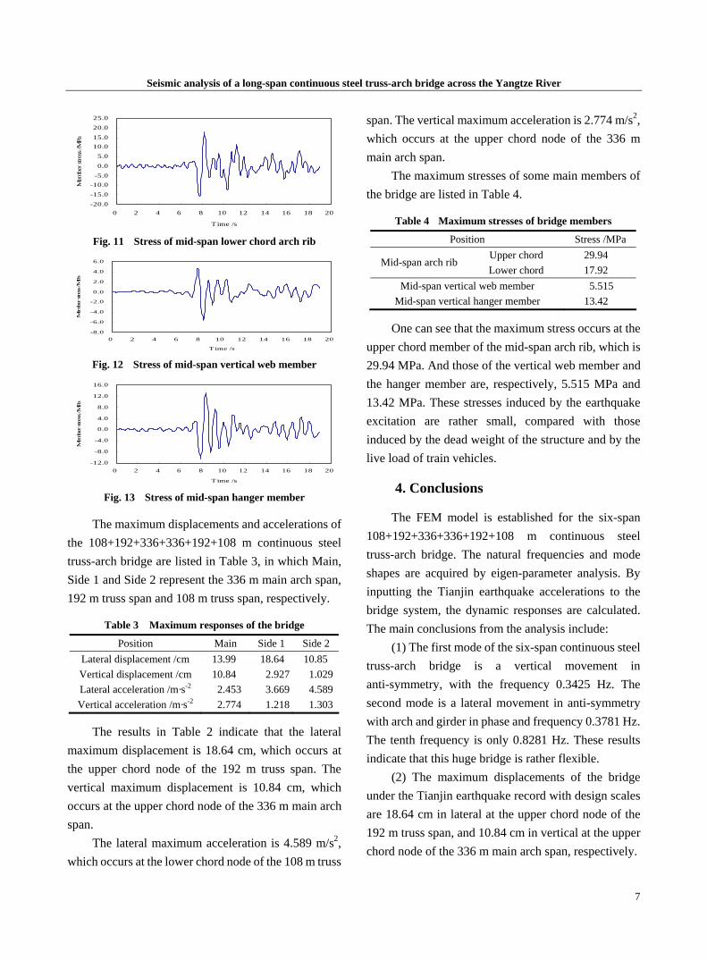
Fig. 10-Fig. 13 are showing the time histories of the stresses of the upper and lower chord arch rib members, the vertical web member and the hanger member at the mid-span of the main arch.
-30.0-24.0-18.0-12.0
-6.00.06.0
12.018.024.030.036.0
0 2 4 6 8 10 12 14 16 18 20
Time /s
Mem
ber s
tress
/MPa
Fig. 10 Stress of mid-span upper chord arch rib
Seismic analysis of a long-span continuous steel truss-arch bridge across the Yangtze River
7
-20.0-15.0-10.0
-5.00.05.0
10.015.020.025.0
0 2 4 6 8 10 12 14 16 18 20
Time /s
Mem
ber s
tress
/MPa
Fig. 11 Stress of mid-span lower chord arch rib
-8.0
-6.0
-4.0
-2.0
0.0
2.0
4.0
6.0
0 2 4 6 8 10 12 14 16 18 20
Time /s
Mem
ber s
tress /M
Pa
Fig. 12 Stress of mid-span vertical web member
-12.0
-8.0
-4.0
0.0
4.0
8.0
12.0
16.0
0 2 4 6 8 10 12 14 16 18 20
Time /s
Mem
ber s
tress /M
Pa
Fig. 13 Stress of mid-span hanger member
The maximum displacements and accelerations of the 108+192+336+336+192+108 m continuous steel truss-arch bridge are listed in Table 3, in which Main, Side 1 and Side 2 represent the 336 m main arch span, 192 m truss span and 108 m truss span, respectively.
Table 3 Maximum responses of the bridge
Position Main Side 1 Side 2Lateral displacement /cm 13.99 18.64 10.85 Vertical displacement /cm 10.84 2.927 1.029Lateral acceleration /m·s-2 2.453 3.669 4.589Vertical acceleration /m·s-2 2.774 1.218 1.303
The results in Table 2 indicate that the lateral maximum displacement is 18.64 cm, which occurs at the upper chord node of the 192 m truss span. The vertical maximum displacement is 10.84 cm, which occurs at the upper chord node of the 336 m main arch span.
The lateral maximum acceleration is 4.589 m/s2, which occurs at the lower chord node of the 108 m truss
span. The vertical maximum acceleration is 2.774 m/s2, which occurs at the upper chord node of the 336 m main arch span.
The maximum stresses of some main members of the bridge are listed in Table 4.
Table 4 Maximum stresses of bridge members
Position Stress /MPaUpper chord 29.94
Mid-span arch ribLower chord 17.92
Mid-span vertical web member 5.515 Mid-span vertical hanger member 13.42
One can see that the maximum stress occurs at the upper chord member of the mid-span arch rib, which is 29.94 MPa. And those of the vertical web member and the hanger member are, respectively, 5.515 MPa and 13.42 MPa. These stresses induced by the earthquake excitation are rather small, compared with those induced by the dead weight of the structure and by the live load of train vehicles.
4. Conclusions
The FEM model is established for the six-span 108+192+336+336+192+108 m continuous steel truss-arch bridge. The natural frequencies and mode shapes are acquired by eigen-parameter analysis. By inputting the Tianjin earthquake accelerations to the bridge system, the dynamic responses are calculated. The main conclusions from the analysis include:
(1) The first mode of the six-span continuous steel truss-arch bridge is a vertical movement in anti-symmetry, with the frequency 0.3425 Hz. The second mode is a lateral movement in anti-symmetry with arch and girder in phase and frequency 0.3781 Hz. The tenth frequency is only 0.8281 Hz. These results indicate that this huge bridge is rather flexible.
(2) The maximum displacements of the bridge under the Tianjin earthquake record with design scales are 18.64 cm in lateral at the upper chord node of the 192 m truss span, and 10.84 cm in vertical at the upper chord node of the 336 m main arch span, respectively.
Seismic analysis of a long-span continuous steel truss-arch bridge across the Yangtze River
8
(3) The maximum accelerations of the bridge under the Tianjin earthquake record with design scales are 4.589 m/ s2 in lateral at the lower chord node of the 108 m truss span, and 2.774 m/s2 in vertical at the upper chord node of the 336 m main arch span, respectively.
(4) The maximum stresses excited by the seismic excitation with design scales are 29.94 MPa in the arch rib member, 5.515 MPa in the vertical web member and 13.42 MPa in the hanger member, respectively, which are rather small compared with those induced by the dead weight of the structure and by the live load of train vehicles.
References: [1] ZHENG J.. High-speed Railway Bridges in China. Beijing:
Higher Education Press, 2008. [2] Cheung, M. S., Lau, D. T. and Li W. C.. Recent
developments on computer bridge analysis and design. Progress in Structural Engineering and Materials, 2000, 2(3): 376-385.
[3] Tseng, W. S. and Penzien, J.. Seismic analysis of long multiple-span highway bridges. Earthquake Engineering & Structural Dynamics, 1975, 4(1): 1-24.
[4] Abdel-Ghaffar, A. M. and Masri, S. F.. Seismic performance evaluation of suspension bridge. Earthquake Engineering, Proc. of 10th World Conference, 1992: 332-338.
[5] Dumanoglu, A. A. and Severn, R. T.. Stochastic response of suspension bridges to earthquake forces. Earthquake Engineering & Structural Dynamics, 1990, 19(1): 133-152.
[6] Dumanoglu, A. A., Brownjohn, J. M. W. and Severn R. T.. Seismic analysis of the fatih sultan mehmet (second Bosporus) suspension bridge. Earthquake Engineering & Structural Dynamics, 1992, 21(10): 81-906.
[7] Saiidi, M., Maragakis, E. and Connor, D. O.. Seismic performance of the Madrone bridge during the 1989. Loma Prieta Earthquake Structural Engineering Review, 1995, 7(3): 219-230.
[8] ZHU D. S. and LAO Y. C.. Selection of input earthquake waves for seismic analysis of bridges. Bridge Construction, 2000, 3: 1-4.
[9] Lupoi, A., Franchin, P., Pinto, P. E. and Monti, G.. Seismic design of bridges accounting for spatial variability of ground motion. Earthquake Engineering and Structural Dynamics, 2005, 34(4-5): 327-348.
[10] Ribeiro, D., Calçada, R., Delgado R.. Dynamic analysis of alcácer do sal railway bridge. Proc. of EURODYN 2005, Paris, 2005: 1661-1667.
[11] Kim, C. W. and Kawatani, M. O.. Effect of train dynamics on seismic response of steel monorail bridges under moderate ground motion. Earthquake Engineering and Structural Dynamics, 2006, 35(10): 1225-1245.
[12] CAO Y. R. and ZHONG T. Y. Seismic analysis of long-span a cable-stayed bridge. Railway Construction, 2007, 47(5): 23-26.
[13] GUO X. and YANG Z. Y.. Seismic resistance analysis of a steel tubular concrete arch bridge based on ANSYS. Railway Standard Design, 2003, 4: 88-92.
[14] Usami, T., LU Z. H, GE H. B. and Kono, T.. Seismic performance evaluation of steel arch bridges against major earthquakes. Part 1: dynamic analysis approach. Earthquake Engineering & Structural Dynamics, 2004, 33(14): 1337-1354.
[15] LI J. B. and GE J.. Seismic analysis of a 5-span half-through CFST arch bridge. World Earthquake Engineering, 2005, 25(3): 110-115.
[16] XU S. Z. and JI T. G.. Seismic performance analysis of a large-span RC arch bridge. World Earthquake Engineering, 2006, 22(4): 74-79.
[17] Galvín, P. and Domínguez, J.. Dynamic analysis of a cable-stayed steel arch bridge. J. of Constructional Steel Research, 2007, 63(8): 1024-1035.
[18] ZHAO C. H. and LI Q.. Seismic response analysis of continuous rigid-frame arch bridge. Bridge Construction, 2007, 32(1): 21-24.
(Edited by Jenny)
May 2009, Volume 3, No.5 (Serial No.18) Journal of Civil Engineering and Architecture, ISSN 1934-7359, USA
9
3D building modeling: A critical investigation practice to learning,
analyzing and deconstruting architecture
Andrea Cammarata (DiAP-Department of Architecture and Planning, Politecnico di Milano, Piazza Leonardo da Vinci 32, Milan 20133, Italy)
Abstract: The research deal with the reconstruction through digital 3D CAAD (Computer Aided Architectural Design) modeling of masterpieces of modern and contemporary architecture. The charm of reconstruction through digital modeling is far less than that of work done on traditional maquette, indeed, makes much deeper level of detail and specificity from knowing. We had to know many technical characteristics of the buildings beyond size, like static-structural features, physical features, economic features and others. In this way the model become real-simulation, a simulated architectural model in all aspects. In addition to these aspects we deeply analyze also the formal, morphological, historical and architectural aspects. The idea is to revitalize and re-discover the logics and the rules of the projected constructions that the designer architect have invented for each masterpiece of architecture, through the comprehension of how is done. The proportional analysis of the modularity on which the design is based is mandatory subject of investigation. Key words: representation; analysis; 3D; modularity; model; architecture
1. Background
The Politecnico di Milano was established in 1863 by scholars and entrepreneurs. Over the years, it has been the home-institution to most prominent professors, including several Nobel Prize winners.
The Politecnico di Milano has approximately 40,000 students and more than 1200 professors as permanent staff in its seven campuses located in the Lombardy Region, organized in seventeen departments of nine networked schools, which makes it the largest institution in Italy for engineering, architecture and industrial design.
Andrea Cammarata, professor; research fields: representation,
CAAD, digital modeling. E-mail: [email protected].
The School of Architecture and Society is located at the Leonardo Campus in the center of Milan and at Piacenza. The Leonardo Campus is the historical seat of Politecnico di Milano since 1927, with most of the academic activities taking place inside this original core of the campus. The new Piacenza Campus represents the latest development of the Politecnico di Milano.
Today, research is increasingly and more closely connected to teaching and represents a priority commitment which makes it possible for us to attain high level results at international level. Research work goes hand in hand with cooperation and alliances with the industrial system[1].
We always think that knowing the world where one will work is a fundamental requirement of students’ training. Being confronted with the needs of manufacturing, industrial and public administration sectors helps research to approach new terrain and to meet the need for constant and rapid innovation. Such an alliance with the industrial sector not only permits the university to continue along its traditional areas but also acts as a stimulus for their development.
This paper deals with a research carried out by the CoDE (Cooperative Design Environment) Lab with the students of the “3D Parametric CAAD Design” class (Leonardo Campus-Milano) and “Digital Design Drawing” (Arata Campus-Piacenza), with trainees and dissertationists.
Both classes deal with all the subjects concerning CAAD-assisted design, with the aim of teaching students how to work autonomously from the

3D building modeling: A critical investigation practice to learning, analyzing and deconstruting architecture
10
analytical pre-planning phase to the final rendering of the artifact. The most frequently used programs are: Autodesk Revit, Graphisoft Archicad and Nemetschek Allplan.
The workgroup, reporting to the Italian Chapter of IAI (International Alliance for Interoperability), relies on the cooperation of qualified professionals.
2. Teaching method
Subjects of analysis and reconstruction were not the projects, but the already created buildings that supply a wider choice of sources and information[2]. We analyzed the formal, morphological, historical and architectural aspects.
For the time being we only deal with Aalto, Ando, Botta, Bottoni (Fig. 1), Holl (Fig. 2), Isozaki, Kahn, Le Corbusier, Meier (Fig. 3), Mies van der Rohe, Niemeyer, Ponti, Terragni and Wright. Soon we will add to the list of possible choice Eisenman, Nouvel, Siza and Venturi.
Fig. 1 Piero Bottoni-Ina building (Marescotti)
Fig. 2 Steven Holl-Chapel of St. Ignatius (Donelli)
Fig. 3 Richard Meier-Royal Dutch Papers Mills
headquarters (Ni Ya)
The teaching method works like this: once the students have learned to use in deep detail the CAAD modeler, they are invited to choose from a list of works (prepared by the teachers) that cover the whole activity of several architects (those above).
Each student must choose a different architecture and search for, with our supervision and direction, all the necessary information and documentation to interpret and reproduce the object.
Also, the material must be sufficiently comprehensive to fully understand the foundational principles of the building, both from the morphological point of view, and from the structural, formal and functional.
The representation of a building only from the visual point of view, so as it seems equal to the original, has absolutely no interest in the course and for the research group.
Thereafter, each single job is supervised with a series of revisions to assist the interpretation stage, where students are often lacking, to route correctly to ensure that the work will not be superficial.
When the architectural model is correctly finished the students submit it to the teachers and to the whole classroom, highlighting features and peculiarities, in ways that I will clarify later.
The research group had refined this type of approach for several years with academic results that gradually improve quality and interest.
3D building modeling: A critical investigation practice to learning, analyzing and deconstruting architecture
11
The CAAD Digital Model Archive of CoDE Lab, directed by Andrea Cammarata, presently boasts approximately 250 models generated by means of different techniques and programs, and with different matter-formal investigation levels.
3. Methodology approach
A significant model of this search could be Peter Eisenman’ study “Ten canonical buildings 1950-2000”[3], where some significant modern architecture works are analytically “deconstructed” in order to restore the logics governing their “construction”. This type of cognitive operation is at the same time a planning operation, since it “rebuilds” the invisible plot of the conceptual order sustaining the designed and possibly built work. Such operation is all the more feasible because the architecture refers to a recognizable order principle.
That’s how the choice of certain works by these authors as quite significant case studies is justified for a disassembly and re-assembly operation of the “constituent” logics supporting them.
With reference to Eisenman’s study again, these architectures can be defined as “canonical”, meaning “the history of architecture as a continual and unremitting assault on what has been thought to be the persistence of architecture: subject/object, figure/ground, solid/void, and the part-to-whole relationship”.
These concepts are now canonical starting from our authors’ work: their works have therefore become canonical too.
“Rather, the idea of the canonical begins to describe potential methods of analysis, which derive from an interest in reading architecture in a more flexible and less dogmatic way”.
As we all know, the “theory of proportions” is not just a branch of mathematics and geometry: it has long been the foundation of architectural design, until the modern movement depreciated it as a residual of
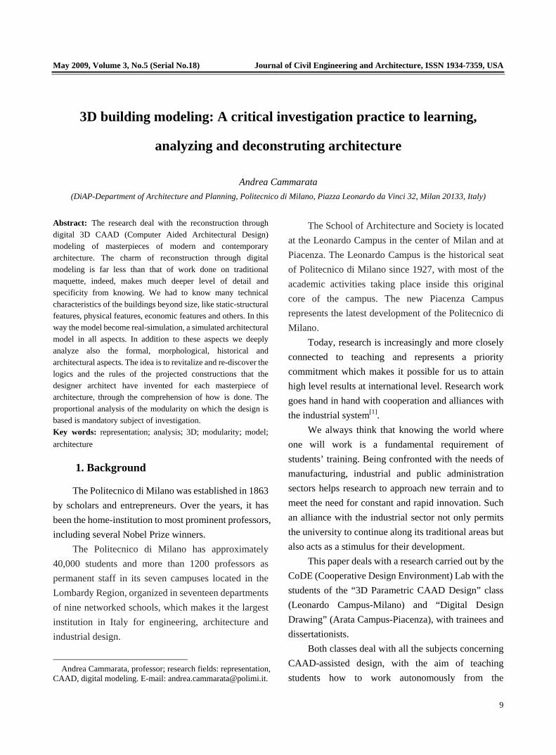
academic architecture (Fig. 4 is showing the 3D model of Richard Meier-Exhibition and Assembly Hall ).
Fig. 4 Richard Meier-Exhibition and Assembly
Hall (Michael Angelo Albert)
But Le Corbusier[4] was still using a proportional measure system based on the harmonious ratio of the human body’s measures. This system was not as much based on the theorems of scientific disciplines as it was on the tradition of architectural and artistic culture, from Vitruvio to Leonardo.
But our reference can still be Eisenman, not only for referring to the above-mentioned “rule” concept, but also for using the “close reading” concept. This is how he explains it: “Colin Rowe[5] first taught me how to see what was not present in a building. Rowe did not want me to describe what I could actually see: for example, a three-story building with a rusticated base, increasingly less rustication in each of its upper stories, and with ABCBA proportional harmonics across the façade, etc.. Rather, Rowe wanted me to see what ideas were implied by what was physically present. In other words, less a concern for what the eye sees–the optical–and more for what the mind see–the visual[6]. This latter idea of “seeing with the mind” is called here “close reading”.
What exactly is the meaning of “close reading”? Or, as Eisenman put it: “close reading of what?” A possible answer that we consider significant is the following: “Close reading can be said to define what has been known until now as the history of architecture. But for our purpose here, close reading also suggests

3D building modeling: A critical investigation practice to learning, analyzing and deconstruting architecture
12
that a building has been “written” in such a way as to demand such a reading.” In other words, “close reading” concerns what the author calls “critical architectural ideas”, which must be seized not in the “optical” coexistent elements of the works, but in the “visual” ones. The distribution is explicit: “Visuality does not refer to a prime facie response to image, but rather to what is apparent and implied by aspects of the building’s formal organization.”
Only the decomposition and recomposition of this modular language-through a computer-assisted “close reading”-accounts for the “architectural ideas” conveyed by Serlio in his project, highlighted here for the first time. (Fig. 5 shows the 3D model of Ludwig Mies Van Der Roth Bacardi Office building).
Fig. 5 Ludwig Mies Van Der Roth Bacardi
Office building (Marinaro)
The newest idea is therefore to revitalize and re-discover the construction of maquettes through the use of digital instruments. This digital 3D models are “real” simulation of existing buildings made by contemporary or modern most famous architects.
The charm of reconstruction through digital modeling is far less than that of work done on traditional maquette, indeed, makes much deeper level of detail and specificity from knowing.
The fact that it’s not applicable on the concept of “scale representation” increase dramatically the level of details that can be achieved can be infinitely more than a traditional maquette.
From this point of view the models are greatly different. In some cases, for example, we have analyzed in detail including all the decorations and the
furnishing of the house. Usually this happens with buildings in which the foundational logic that governs the project went up to the definition of the interior, involving every part as an active and an important part of the creative project. The most interesting samples are Frank Lloyd Wright’ building.
Sometimes, however, we found much more interesting to investigate the technological equipment (plant), especially when they become drivers of the overall design process. There are many cases of this kind of study, for example, the modular systems from Le Corbusier and Mies van der Rohe period until recent years. (Fig. 6 shows the 3D model of Botta-Cymbalist Synagogue and Jewis Heritage Center).
Fig. 6 Botta-Cymbalist Synagogue and
Jewis Heritage Center (Dardanelli)
Still different cases are those in which the building is very wide. In these cases the job is mostly focused on to put in evidence the project in its fundamental characteristics, that in the perfect reproduction of every part and/or component of the structure. Often besides, in the case of great buildings, as in the case of buildings turned to particular purposes, are missing a lot of information. Generally documentation is easily found

3D building modeling: A critical investigation practice to learning, analyzing and deconstruting architecture
13
on the first and last floor, along with the standard, often hypothetical.
In this sense we have always given priority to understand and focus on the modeling project, the generative scheme, rather than the perfect reproduction of all the details.
We can also investigate and understand in detail many more aspects that in a maquette is not possible to properly highlighted.
The single objects that are components (part of) the model are simulation of architectural elements. We know many technical characteristics of them beyond size, like static-structural features, physical features, economic features and others.
The set of characteristics of individual objects that make up the model, if properly placed in relation to each other, give us an interactive digital model, which itself has the same physical nature, and can be subjected to simulated action/reaction very specific interest. (Fig. 7 shows the 3D model of Richard Meier- Rickmers Reederei Headquarters).
Fig. 7 Richard Meier-Rickmers Reederei
Headquarters (Piana)
Several research and thesis are going on right now in accord and in collaboration with some colleagues to highlight other aspects that do not normally become part of traditional learning, but these tools make it very fascinating to look into.
Among these we quote case studies of historical reconstructions, sustainable architecture, estimated metric calculation, virtual yard and structural calculation. Such experimentations are developed in close collaboration with the manufacturing software
houses, usually very interested to the intensive testing that we do and, above all, to the dissemination and integration in the didactics. Their support is essential to always have the most updated version available.
For instance, in some recent historical studies we have structurally faced a series of buildings structurally based on vaults. Such vaults must laboriously be modeled to one to one with a specific 3D modeler.
Despite this, once passed the ended model to the program of structural calculation, this has never been able to interpret the element “vault”, doing therefore calculations that gave completely wrong results. This inconsistency was immediately reported to the manufacturing house that will handle to eliminate the problem in a next release of the program.
4. Transformations
The simulation applied to the transformations that some important functionalist buildings have undergone during their existence. Sometimes the changes were due to a difference or adjustment of their intended use, and sometimes the changes were quite substantial and due to design and/or assembly mistakes.
We often just observed the remarkable differences between the designed and the created building.
The lack of information also allows to understand the reasons of the project changes and to assess them from an architectural-methodological viewpoint.
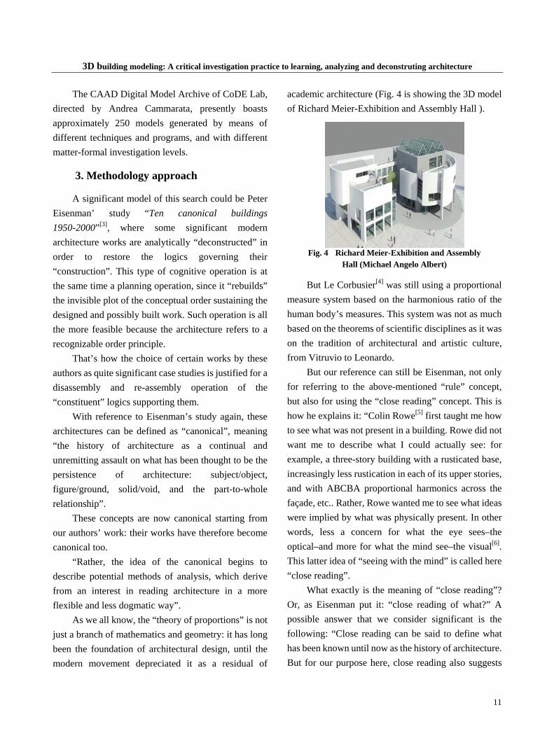
This type of simulation led to a whole series of remarks on the alleged/real flexibility of the analyzed buildings and on the building techniques and technologies of the time, with their pros and cons, and we realized how experimental certain futuristic works were at the time. (Fig. 8 shows the 3D model of Giuseppe Terragni–Novocomum building ).
3D building modeling: A critical investigation practice to learning, analyzing and deconstruting architecture
14
Fig. 8 Giuseppe Terragni–Novocomum
building (Dell’ Acqua)
Most often we can see and understand the modifications that a building has undergone (suffered) during its existence and its history. Time is a great threat to the architecture, but much more often for bad architecture.
The good architecture often shows unusual and unexpected abilities of adaptation to the carelessness of the men and the changes of destinations of use which are submitted.
To let the students to make these operations of comparison is very instructive, also because it teaches them that the architecture before being monument of herself is made of alive objects that, sometimes, are dynamic.
The most modern programs CAADs have features such as the “alterations” and/or the “phases”, that allow to compare the state of the building in two (or more) separate temporal moments, features which have proved valuable in this type of investigation.
5. Project never built or building demolished
As far as created and lost works are concerned, we deepened only certain specific cases that seemed most interesting.
This type of choice is also due to the shortage of traceable sources, thus making the real/virtual barrier too thin: we often had to interpret drafts or drawings that were too partial to deduce the whole object and we
therefore had to reconstruct by subsequent suppositions.
The whole technological aspect of the building would also be further neglected, since in project representations of the past it isn’t always possible to understand and extrapolate the building’s structure, facilities and many constructive details.
Although this operation looks quite interesting, we have not applied it very often, being “non-scientific” and unverifiable.
Instead they are revealing very interesting some experiments in the virtual reconstruction of historic designed buildings never realized.
Such searches, based on authors of the Renaissance, you/they are bringing to the realization of very complex and articulated models, that you/they also receive vast consensus in disciplinary sectors as that of the historians, that generally shown little interest in experimentations of technological character.
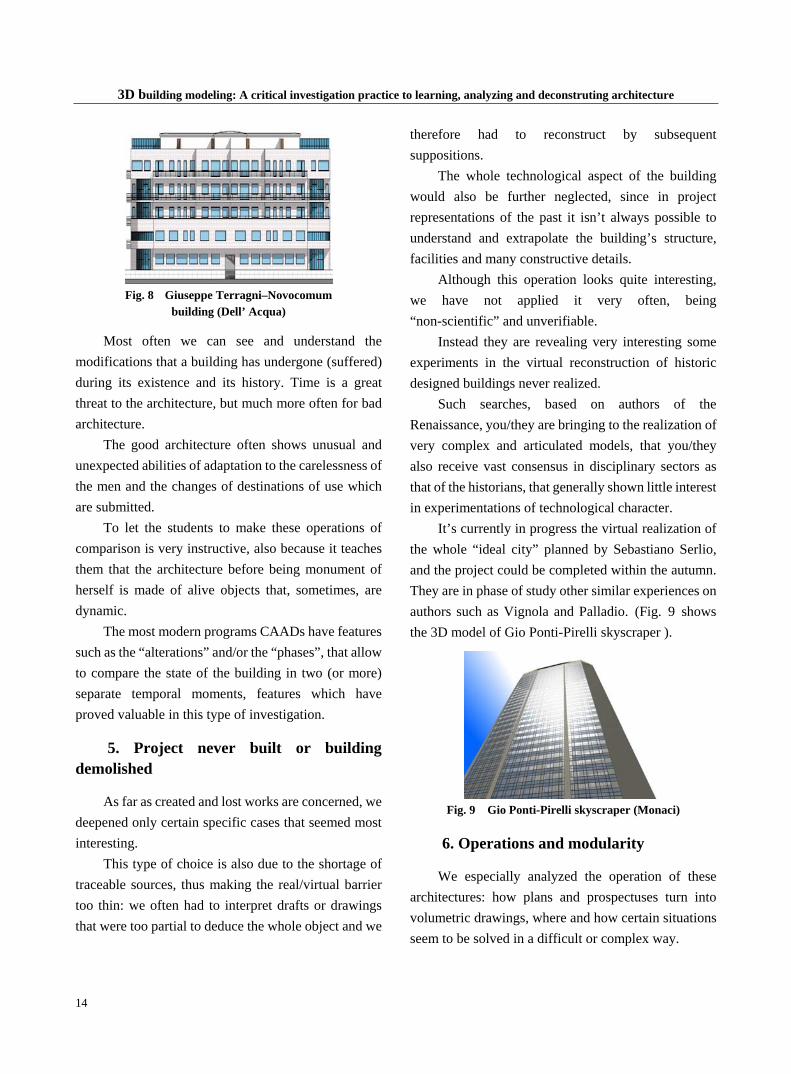
It’s currently in progress the virtual realization of the whole “ideal city” planned by Sebastiano Serlio, and the project could be completed within the autumn. They are in phase of study other similar experiences on authors such as Vignola and Palladio. (Fig. 9 shows the 3D model of Gio Ponti-Pirelli skyscraper ).
Fig. 9 Gio Ponti-Pirelli skyscraper (Monaci)
6. Operations and modularity
We especially analyzed the operation of these architectures: how plans and prospectuses turn into volumetric drawings, where and how certain situations seem to be solved in a difficult or complex way.

3D building modeling: A critical investigation practice to learning, analyzing and deconstruting architecture
15
The constituent proportional analysis of the modularity on which the design is based is another subject we are currently investigating (as already longly said at the beginning of this paper), from masters of the modern movement to contemporary architects.
We are browsing a whole series of works and looking for the expressive language of modular grids and symmetries, thus producing three-dimensional constituent morphological analyses.
Task for students is to find a way to graphic-representative that expresses the concepts of spatial relationships that usually are not obvious or evident. When it comes to represent two-dimensional diagrams, representing how many have already been explored and exploited. In 3D, however, much has still to be done. Both by tradition, which for simplicity is almost always refers to axonometric views, often of the split, which allow us to return to work in 2D to 3D views. Even in this case a field extensively. (Fig. 10 shows the 3D model of Oscar Niemayer-Mondadori building).
Fig. 10 Oscar Niemayer–Mondadori
building (Paderni)
When it comes with representing bidimensional schemes, a lot of representative formalities (modalities) are already been explored and exploit. In 3D instead, very it is still to be done. Both by tradition, and for simplicity is almost always refers to axonometric sights (views), often using 3D sections, that allow us to draw in 2D on 3D sights (views). Also this case it is an area widely investigated and discussed.
Some recent experimentation of important and innovative studies of architecture you/they have shown that the form of the representation of the architecture, it’s architecture itself, contributing in substantial way to the project’ final form.
The research of new expressive forms and investigation of the three-dimensionality is pushing therefore to give new interpretative keys of the form (shape) of the architecture itself, with the hope to rise the students sensibility (tomorrow’s building designer) to the planned (projected) and controlled manipulation of shapes.
A further discussion in this direction is represented by a case study in which we are developing new way for the representation of flows (people, traffic, normal access, situations of maximum crowding, risky situations, etc.) and their visual simulation inside the architectural project.
7. Trends and mathematics
Another fascinating aspect, almost consequential to the previous one, has been the rediscovery of the appeal of certain buildings’ analysis, which-for previous or subsequent analyses-disclosed a trend, a morphology and/or a plasticity shaped on mathematical-physical[7] or proportional elements[8]. The analyses and their computerized audit highlighted some very complex relationships and extraordinary design solutions. (Fig. 11 shows the 3D model of Andrea Palladio–La Rotonda, Villa Cpra).
Fig. 11 Andrea Palladio–La Rotonda,
Villa Cpra (Nemeth)
(to be continued on Page 21)
May 2009, Volume 3, No.5 (Serial No.18) Journal of Civil Engineering and Architecture, ISSN 1934-7359, USA
16
Underground water biological field’s variation and
geoenvironmental safety in city*
YI Nian-ping, ZHANG Xin-gui, WANG Yang, HUANG Jun-peng (College of Civil and Architectural Engineering, Guangxi University, Nanning 530004, China)
Abstract: In the process of city construction, as a comprised factor of city geological environment, underground water takes the most active part, and its dynamic change is fiercest. The city construction unceasingly disturbs underground water chemical, dynamical, physical and biological field. In return, the four fields’ changes also can affect the geological environment that city lived by, in other words they affect safety and stability of geological environment. Interaction of underground water and the geoenvironment directly displays in the following two ways: The first is that the underground water and the geological body transfer the energy each other; the second is that the strength balance of geological body is broken. Underground water variation brought about by city construction is the factor which cannot be neglected. Underground water variation on the one hand changes soils or rocks’ physical, biological, chemical and mechanical properties, then influences the deformation and strength of geological body. On the other hand it changes its own physical, chemical properties and biochemical component. At present, from mechanics aspect, interaction between chemical field and biological field variation of the underground water and the geological body lacks research. Although interaction between them is long-term, slow, but when it compared with water-soil or water-rock interaction in the entire process of formation of rocks or soils or geologic evolution history, the qualitative change of the biological and chemical action of rocks or soils brought about by city construction is remarkable. In this paper, aiming at underground water biological field factor which is easily neglected by people, it analyzes that underground water biological field affects possible mechanism and approach of properties variation of rocks or soils
* Acknowledgments: This work is keystone items of Ministry of Education P.R.C (No. [2003]77), National Natural Science Foundation of China (No. 40062002), Natural Science Foundation of Guangxi (Nos. 0447001, 0249010, 0575019, 0779012, 0632006-1B, RC2007001) and Department of Water Resources of Guangxi (No. [2004]4).
Corresponding author: YI Nian-ping (1966- ), female, senior engineer; research fields: geological environment and engineering, geotechnical engineering. E-mail: [email protected].
in city construction, brings forward further research method and development direction have been also proposed. Key words: underground water; biological field; microscopic structure
1. Introduction
In the process of city construction, as a comprised factor of the city geology environment, underground water takes the most active part, and its dynamic change is fiercest, so it becomes the outstanding one of multitudinous factors that initiates the city geology disaster and the geology effect of correlative environment. The city construction on the one hand remolds the soil characteristic, on the other hand also imposes all kinds of loads to the soil body, it unceasingly disturbs the chemical, dynamical, physical and biological field of underground water. Meanwhile it arouses four actions in the soil body: The physical action (includes lubricating, soft and sloughy action, strengthened action of hygroscopic water), chemical action (includes exchange of ionic, dissolution, hydration, hydrolysis, corrosion, oxidation and deoxidation, precipitation), mechanics action (includes seepage, seepage flow, pore water pressure and water dynamic pressure, uplift pressure, frozen-heave force, as well as one kind of matrix suction in unsaturated soil) and the biological action (biological absorption, transformation, elimination, degeneration and reaction of chemical composition). The interaction of underground water and the geological body directly displays as following: The first is that the underground water and the geological body factors transfer the

Underground water biological field’s variation and geoenvironmental safety in city
17
energy. The second is that the strength balance of geological body is broken. The third is that biochemical component of the underground water will be changed. Underground water variation on the one hand changes the physical, biological, chemical and mechanical properties of rocks or soils, then influences the deformation and strength of geotechnical body. On the other hand it also changes the physical, mechanical properties and the biochemical component of underground water. Although interaction with them is long-term, slow, but when compared with water-soil or water-rock interaction in the entire process of formation of rocks or soils or geologic evolutional history, biological or chemical action are remarkable in terms of water-soil or water-rock interaction that city construction brought about. The biological influence is a factor which cannot be neglected, as the aquatic environmental variation and chemical variation affects mutually, its change is still remarkable.
As the development of city construction, the massive use of three industrial wastes, greenhouse gas discharging, household garbage piling up and filling, chemical fertilizer, agricultural chemicals cause serious pollution of underground water, soil mass and atmosphere, affects structure and properties of soil through water-soil action, and destructs water-soil biology and the ecosystem environment, and finally, through the water as carrier and solvent, the physical climate system and the biochemistry circulatory system, cause the mutual action of the telluric stratums. Because of increase of project activity and some unreasonable exploitation ways of underground water, the condition of surface drainage and seepage flow is changed, equilibrium cycles of surface water, underground water and atmosphere precipitation are destroyed, the four field structures of underground water are transferred, and the influence of biological field variation is even more prominent. The influence that underground aquatic biological field variation to the soil body stability involves the geotechnical engineering, hydrology geochemistry, biology,
environment geology and so on, and its research can better consummate and develop water and soil interaction theory.
2. Factors of undergroundwater biological field variations
The underground water biological field mainly refers to the environment of each biotic factorial action which generally includes the botanic and microorganic action. We mainly discuss the influence of microorganic function. The microorganism is an organism which the naked eye cannot catch, including the bacterium, mycelium microorganism, the fungus that contain no chlorophyll, the algae contains chlorophyll, the protozoon and the super-microorganism, whose structure is smaller than the bacterium, which can not be found even under the microscope[1]. The underground water that opens the structure, richly contains each kind of microorganism group. In the half-opened structural water, there mainly lives the anaerobe. The underground water structure whose hydrological geology was sealed generally lacks the microorganism. Soils or rocks also usually include microorganisms of all kinds, like the bacterium, the fungus and the emission fungus. Bacterium is the most, the emission fungus is less, the fungus is the least. The microorganic function is controlled by quantity and temperature of organism, hardness index and ingredient as well as vicissitudinary intensity of water. The primary factors that cause the underground water biological field variation include:
(1) The function that excessive exploitation of underground water which caused by city construction, excavations, transports, piles and fills of soil, telluric surface processing and so on, have directly changed the environment of microorganism growing in underground water and soil mass.
(2) The discharging of three industrial wastes, greenhouse gas, creates the greenhouse effect and
Underground water biological field’s variation and geoenvironmental safety in city
18
climate vicissitude, changes the soil mass and microorganic habitat in underground water.
(3) The discharge of three types of wastes, causes the pollution of the city ecosystem, microorganism species that are adapt to the polluted environment to leave and propagate massively, but species that are not is on the verge of extinction, or even extinct. The decrease of microorganism species and the increase of the microorganism quantity cause the influence, even the variation of the biologic environment of underground water.
(4) The activities of city construction changes the drainage, supply, seepage-flow condition and hydraulic relationship of underground water, accelerates the process of the pollution of underground water and causes the change of biochemistry environment of water. The change of hydraulic condition causes the transformation of pattern of the microorganism migration and the microorganism distribution in underground water.
(5) Factors such as Engineering construction, environmental variation and so on cause the disorder of the structure of soil mass, the fluctuation of the number of grain structure, the change of the quantity and distribution of the pore, the strengthening of hydraulic conductivity and air permeability between the big pores, which are extremely advantageous to microorganisms’ activities. There lives massive aerobic microorganisms on the water film of big pores and anaerobic microorganisms in the small pore. But in the extremely fine pore, which bacterium cannot enter in, the organisms are able to be preserved. The structural destruction causes the variation of the activeness and the distribution of the microorganisms in the soil as well as the indirect influence of the underground water biological environment which flows through the soil body.
3. Soil body stability effect caused by underground water biology field variation
The interaction, influence, exchange, seepage between microbial populations in underground water and soil mass environment and the influence of soil body stability created by biotic factors in the underground water were mainly aroused by the absorption and degeneration of the contaminative substances in the underground water and the soil body done by the microorganisms or organisms in the water. Then the chemical component and mutual action in the water and soil body, microstructure as well as the physical characteristic and mechanical properties of soil mass are changed. Through the long-term water-soil interaction, the quantitative change will cause qualitative change.
Take the Benzene as an example to understand the microbial degeneration characteristic, to analyze how they affect chemical composition variation of the underground water and the soil microscopic structure and then influence the stability of the soil body.
(1) Oxygen-needed degeneration. In oxygenous environments, nearly all petroleum pollutants can be degenerated and O2 is this kind of acceptor in degeneration process. Take the aromatic benzene as the example, its mineralized equation is[2]:
C6H5-CH3+9O2→7CO2+4H2O (1) (2) Desulphurization degeneration. As researches
indicate, when some electron acceptor whose oxidized ability is strong was consumed, SO4
2- may replace the anaerobic microorganism to degenerate the electron acceptor of the hydrocarbon pollutant. Regarding benzene, its reaction equation is[2]:
C6H5-CH3+4.5 SO42-+3 H2O
→2.25H2S+2.25HS-+7HCO3-+0.25H+ (2)
(3) Denitration degeneration. When the dissolved oxygen in the water-bearing stratum is almost consumed away, the anaerobic microorganism uses NO3
- to replace O2 as the final electron acceptor, to carry on the hydrocarbon degeneration. Regarding benzene, its reaction equation is[2]:
Underground water biological field’s variation and geoenvironmental safety in city
19
C6H5-CH3+7.2H++7.2NO3-
→7CO2+7.6H2O+3.6N2 (3) We can see from the above reaction equations that
the biodegradation can transform the harmful pollutant to nearly harmless product. In reaction (1), whether it can carry on is decided by the content of dissolved oxygen in underground water. The higher the content of dissolved oxygen is, the easier reaction will carry on, the more CO2 will be produced. In the region where oxygen content is sufficient in underground water, on the intersurface of soil and water, the fractional pressure and heightenning of CO2 can urge dissolution to the calcite, the dolomite, the magnesite and the calcareous cement in the medium. This causes the content of Ca2+, the Mg2+ in the underground water and hardness of underground water increase. As the water migration impetus circulation of chemical composition, the macroscopic intensity of soil can weaken gradually. Although this kind of action seems week, the reaction is carried on continuously and CO2 is produced unceasingly. Especially the region that benzene pollution is serious and the oxygen content is sufficient, is so. In the reaction (2), SO4
2- can be consumed unceasingly. The SO4
2- in the underground water play an extremely vital role in fluorine migration, the more SO4
2- are, the more advantageous to the fluorine migration it is. It can displace the fluorine ion in the stratum, cause the fluorine content in the underground water increase and create the fluoride to concentrate in the underground water. The research results of literature[2] indicate that the fluorine pollution may cause the stability of soil colloid be senhanced, and it does not favor the clay soil to gather and deposit. This does not make for the formation of good soil structure and is easy to cause other pollution matters to shift along with the soil colloid flowing, which will make the pollution scope expand and the pollution degree aggravate. Obviously, in the soil belt that fluorine pollution is serious, without doubt the reduction of SO4
2- quantity can attenuate the occurrence of this kind of displacement process, enormously eliminate the
normal effect produced by the structural property due to the formation displacement and restrain the fluorine migration in underground water and a series of geological and environmental effects which are caused by itself. Moreover, H+ and H2S that are produced in reaction, cause the pH value of the underground water to reduce, be acid, which brings certain corrosion action to soil mineral ingredient. Reaction (3) consums NO3
- and H+, the pH value of water elevates. In environment of anaerobic underground water,
the microorganisms also may use hydroxide or the oxide of iron in the environment as the electron acceptor, namely:
C6H5-CH3+36Fe(OH)3+72H+ →7CO2+36Fe2++94H2O (4)
In the stage that Fe(OH)3 colloids which is adsorbed on soil skeleton is deoxidized to the form of Fe2+, where soil is in the environment of deoxidization, the colloids Fe3+ that are already softened and include massive hygroscopic waters are deoxidized to Fe2+ which are easily dissolved. The disappearance of organic matter and iron colloid which bear enormous specific surface area in the soil causes the surface energy of soil drop largely, hygroscopic water reduce, and meanwhile, Fe2+ increase in the solution, the double electric layer of soil grain become thinner, grain gather and deposit easily, the diameter of particle become larger and the internal friction angle of soil mass increase. The acidity of water-soil system is slightly reduced. In addition, the research results of literature[4] indicate that, under existence of organic matter, the microorganism in soil and water, because their vital activities need massive oxygen, causes electric potential of oxidation and deoxidization in the system to reduce, Fe3+ that dissociates in ferric oxide gradually to be deoxidized to Fe2+. At the same time the biological enzyme that is produced in the microorganism activities and the organic acid that is produced in the decomposition of organic matter, can also promote the oxidation and reduction reaction to carry on smoothly. Therefore, the ferric oxide as

Underground water biological field’s variation and geoenvironmental safety in city
20
cementation that dissociates in the soil will unceasingly activate and drain, the physics and mechanical properties of soil can go down slowly.
The biological adsorption also is the factor which cannot be neglected. There are lots of waste water or solid rejects contain heavy metal ions like arsenic, cadmium, chromium, copper, mercury, nickel, lead, selenium, zinc that are produced in the process of industrial production, which are the pollution source, that are extremely harmful to the ecosystem. The soil layers clean the heavy metal in the polluted water in the function of capture like adsorption, which can possibly cause the heavy metal accumulation in the soil and change its own constitutive property. From the studies of people, we can discover that microorganism like the bacterium, the fungus, the algae and so on in the underground water, can adsorb or concentrate the heavy metal and reduce the influence of heavy metal pollution source to the soils or rocks in the process of the underground water migration. The biological adsorption of the heavy metal ions mainly include the electrostatic attraction, the complexing, the chela gathers, ionic exchange, micro precipitation, oxidation and reduction reaction, and so on, whose mechanism is complex and is the current hotspot of the research. The effect of biological adsorption mainly depends on many factors like the pH value, the temperature, the diameter of absorbent particle, the adsorption time and the initial concentration of heavy metal ion etc. The adsorption of microorganism in underground water, on the one hand weakens the pollution of water and soil caused by heavy metal ions, on the other hand, weakens or even eliminates the action, which is created by heavy metal ions. These heavy metal ions initiate the chemical reactions through contact of water and soil to change the microscopic structures and physics mechanical properties of rocks or soils. Although this action is extremely weak, the accumulative effect of this kind of action cannot be neglected, because the process of the interaction between underground water and soil is extraordinarily long. Looking from this
point, the biodegradation or all other correlative biological actions is so. Under the combined actions of all biological effects of the underground water, it will finally affect the structural strength of soil mass.
4. Conclusions
Interaction between underground water and soil body is a complex system where its factors affect each other. The influence of underground water to soil body includes four aspects, physical, mechanical, chemical and biological. This paper, from aspect of biological action, focuses on the influences of soil stability caused by the variation of underground biological field. At present, the correlative literatures mainly concentrate on the aspects of dynamical and physical field variation. Researches of chemical field variation were begun in the recent years and that to the field of biologic field variation were less compared to the chemistry field. Focusing on the present situation of serious pollution of the underground water the urbanized development brought about, the influence of biological action of underground water on soil structure increasingly bears the important practical significance, and the scope of exploration and research may be wider.
When studying the influence of biological field variation, we should not only limit to the sole process simulation for biological action of underground water and the soil mass. What we should do is to combine the important physical processes of the soil– the properties of rock and soil, the microscopic structure and the four field variations of underground water, and then to carry on the comprehensive analysis, taking the human activities into account. It will be helpful for us to carry on the discussion, research, and discovery on the mechanism of biological field variation, and to deepen the understanding of the interaction of water-soil and carry it further. We can use the method that the theory and the test unite, according to different category natures of microorganism in underground water. From

Underground water biological field’s variation and geoenvironmental safety in city
21
the analysis of the intrinsic factors—the composition of soil mass, the mechanical characteristic, the structural strength and so on, and the external factor—the influence of environmental field, we can take the key factor of the influence, use the existing test methods , establish the suitable simplification pattern, analyze and prove, simulate the biological variation coupling shape of the underground water under certain condition, find its latent engineering significance, combine the influence that city underground water variation to the soil stability and the city safety, provide the advantageous scientific reference for forewarning and the elimination of latent danger of the city that underground water brought about.
References: [1] LI Xue-li. Hydrology Geochemistry. Beijing: Atomic
Energy Publishing House, 1988. (in Chinese) [2] CHEN Yu-dao, ZHU Xue-yu. Hydrocarbon pollutant
mechanism of the ground water biodegradation. Dawu Water Source Guangxi Geology, 1999, 12(2): 12-16. (in Chinese)
[3] XU Zhong-jian, LIU Guang-shen, WANG Hong-yu, LIU Wei-ping. Research on influence of the fluorine pollution to the soil colloid stability. Science of China Environmental, 2002, 22(3): 218-221. (in Chinese)
[4] ZHOU Fang-qin, LUO Hong-xi, WANG Yin-shan. Microorganism to certain geotechnical project nature influences. Journal of Taiyuan Science and Technology University, 2000, 31(1): 26-31. (in Chinese)
(Edited by Jenny)
(continued from Page 15)
References: [1] Banham, R.. The Architecture of the Well-Tempered
Environment, London, 1969. [2] Curtis, W. J. R.. Modern Architecture Since 1900. London,
1996. [3] Eisenman P.. Ten Canonical Buildings 1950-2000. New
York, 2008. [4] Le Corbusier. Vers une Architecture. Paris, 1923. [5] Rowe, C.. The Architecture of Good Intentions: Towards a
Possible Retrospect. Academy Editions, 1994.
[6] Pevsner, N.. Pioneers of Modern Design from William Morris to Walter Gropius. New York, 1949.
[7] Rowe, C.. The Mathematics of the Ideal Villa and Other Essays. Cambridge, MA, 1976.
[8] Tafuri, M., Dal Co, F.. Il Ruolo Dei ‘Maestri’, in Architettura Contemporanea. Milano, 1979.
(Edited by Jenny)
May 2009, Volume 3, No.5 (Serial No.18) Journal of Civil Engineering and Architecture, ISSN 1934-7359, USA
22
A statistically refined Bouc-Wen model for the identification of structures
under tri-directional seismic excitations*
LIN Jeng-wen
(Department of Civil Engineering, Feng Chia University, Taichung 407, Taiwan)
Abstract: This paper presents a statistically refined Bouc-Wen model of tri-axial interactions for the identification of structural systems under tri-directional seismic excitations. Through limited vibration measurements in the National Center for Research on Earthquake Engineering in Taiwan conducting model-based experiments, the 3-D Bouc-Wen model has been statistically and repetitively refined using the 95% confidence interval of the estimated structural parameters to determine their statistical significance in a multiple regression setting. When the parameters’ confidence interval covers the “null” value, it is statistically sustainable to truncate such parameters. The remaining parameters will repetitively undergo such parameter sifting process for model refinement until all the parameters’ statistical significance cannot be further improved. The effectiveness of the refined model has been shown considering the effects of sampling errors, of coupled restoring forces in tri-directions, and of the under-over-parameterization of structural systems. Sifted and estimated parameters such as the stiffness, and its corresponding natural frequency, resulting from the identification methodology developed in this study are carefully observed for system vibration control. Key words: Bouc-Wen model refinement; 95% confidence interval; multiple regression; natural frequency estimation
1. Introduction
System identification for structural health monitoring[1] and damage detection in civil structures is moving to the forefront of worldwide research activities. Such monitoring and detection for buildings and bridges is important for the public safety related to natural disasters such as earthquakes, and is also
* Acknowledgments: This research was sponsored by the National Science Council, Taiwan (No. NSC 96-2221-E-035-038).
LIN Jeng-wen (1970- ), male, Ph.D., assistant professor; research fields: system identification and control, applied economics. E-mail: [email protected].
becoming increasingly important because of the aging of infrastructure systems. Aging infrastructure systems are causing extreme concern in densely populated areas and there is an urgent need for reliable identification systems that are capable of providing an accurate estimation of the safety and of the remaining life of such structures.
Several researchers utilized different methodologies of system identification to extract structural characteristics. For instance, Beck and Jennings[2] determined the optimal estimates of the model parameters by minimizing a selected measure-of-fit between the responses of the structure and the model. Lus, et al[3] proposed methodology which is based on the eigensystem realization algorithm and on the observer/Kalman filter identification approach to perform identification of structural systems using general input-output data via Markov parameters. LIN, et al[4] presented an adaptive on-line parametric identification algorithm based on the variable trace approach for the health monitoring of non-linear hysteretic structures.
Health monitoring has two main applications[5]. One is related to natural disasters such as earthquakes and hurricanes which can damage or destroy civil engineering structures such as buildings and bridges. After such events government engineers must make assessments of the damage/safety of structures. Visual inspection only allows rather limited information about the extent of damage, since damage can easily be present in places that are not visible or accessible. Trying to infer the actual safety of a structure from

A statistically refined Bouc-Wen model for the identification of structures under tri-directional seismic excitations
23
what is visible is risky and inaccurate. System identification methods[6-7] by pass this limitation by assessing damage based on dynamic behavior properties, using dynamic modeling. The second main application is to the aging infrastructure in the US. Many of the roadways and bridges have become old enough that hidden deterioration can be quite serious. One prime example is the Williamsburg Bridge of the New York city, which required very expensive renovation. Hence, this area of research involves both the saving of millions of dollars in replacement of buildings and bridges, and more importantly, an increase in public safety.
In dynamic modeling, however, possible effects of sampling errors, of coupled restoring forces in tri-directions, and of the under- over-parameterization of structures deter successful identification schemes. It would be sophisticated to analyze the identification methodology within a probabilistic framework due to the random nature of environmental loads[6]. In this context, we propose a statistical and nonlinear model parameter refinement approach to the extended Bouc-Wen model of tri-axial interactions so as to simplify the mathematical model for an economic design of system vibration control. First, a model-based experimentation is implemented in which the 3-D Bouc-Wen model is adopted and modified. Next, we apply the resulting nonlinear model parameter refinement approach to evaluate the structural frequency and compared the value obtained with the value of the fast Fourier transform, followed by conclusions of this study.
2. Model-based experimentation and 3-D Bouc-Wen model of tri-axial interactions
One major area of system identification is to promote experimental analyses, where analytical methodologies are tested using recorded data in the field or lab. Important challenges are yet to be confronted: stochastic modeling of nonlinear systems,
uncertainty of measurement, and safety and damage assessment[8]. Thus, we propose a statistical confidence interval based nonlinear model refinement approach and apply it to the un-damped structural system (Fig. 1), i.e. a three-story full scaled steel structure, under 3-D excitations using vibration measurements in the National Center for Research on Earthquake Engineering (NCREE) in Taiwan, conducting model-based experiments. Three strong ground motions (Δt = 0.005 sec) of the 1940 El Centro (California), 1995 Kobe (Japan), and 1999 Chi-Chi (TCU084, Taiwan) earthquakes were given as earthquake loads during the shaking table tests. Time histories of structural accelerations are measured, while structural velocities and displacements are integrated from the corresponding accelerations.
Fig. 1 Model-based experiment in the National Center for Research on Earthquake Engineering (NCREE), Taiwan
The geometry of the structure (Fig. 1) contains a slab-beam-column configuration for each floor (degree of freedom), in which the associated mathematical model possesses a concentrated mass representing the slab and a resistance box representing the beam-column frame. Estimates of the structural mass can be obtained from the geometry of the structure and
A statistically refined Bouc-Wen model for the identification of structures under tri-directional seismic excitations
24
from knowledge of the type of materials. The structure is constructed with materials of steel and concrete with density 7.85 3/ mt and 2.3 3/ mt , respectively. Each floor’s dimension is 4 m × 2.5 m × 11.5 cm, consisted of concrete and supplement with a 6930 kg mass block, while the beam-column frame, for each floor, is equipped with a length of 4.5 m, a width of 3.0 m, and a height of 3.0 m, with the cross-sections of the beams and columns are H200×150×6×9 mm and H200×204×12×12 mm, respectively. After a simple calculation, the masses of the first, second and third floors are 11364.206 kg, 11364.206 kg and 11030.738 kg, respectively.
Since the accuracy of structural identifications highly depends on the adopted system’s model, it is required to establish a reasonable, feasible as well as general description of a nonlinear model that is able to provide the best description of the system’s behavior. However, if no a priori information is available on the type of the structural system, problems related to under-parameterization and over-parameterization will arise[6]. Notice that the case of under-parameterization includes all the cases in which the model used to represent the structural response (e.g. the restoring force) has fewer characterizing parameters than the “real” structural system, while the opposite is true for the case of over-parameterization[6]. In characterizing the system’s characteristics, Juditsky, et al[9] pointed out that the quality of the nonlinear black-box modeling procedure is always a result of a certain trade-off between the “expressive power” (order) of the model we try to identify (the larger the number of parameters used to describe the model, the more flexible is the approximation), and the measurement (stochastic) error (which is proportional to the number of parameters). Such a rapprochement leads to search for an initial flexible model followed by refining it to the extent that cannot be further improved for exact-parameterization of structures as well as economic design of structural vibration control.
The Bouc-Wen model of tri-axial interactions is used to represent the behavior of the structural system (i.e. the shear-type building in Fig. 1). The rigid body motion of the structure under tri-directional excitations contains displacements in the x, y and z directions, and our focus will be on the shear stiffness in the x-y plane. The effects of structural rotation arising from asymmetry of structure or unsymmetrical excitations of structure have been excluded via a synchronous signal check. The remaining factors that affect accurate identifications are sampling errors, coupled restoring forces, and the under-over-parameterization of structures. For convenience, the equation of motion for a single degree of freedom structure can be expressed as:
( ) ( ( ), ( ), ) ( )gmu t r u t u t t mu t+ = −&& & && (1)
Where m denotes the structural mass, )(tu is
the structural displacement, )(tu& is the structural
velocity, )(tu&& is the structural acceleration, and
( )gu t&& is the ground-induced acceleration, while t
indicates the time and )(tr is the restoring force. The mathematical formulation for the variation of the restoring force r over time, i.e. r& is coupled in the x and y shear-directions[10], and it can be expressed, including the effects from the z direction, as:
21 1x x x x x x x x x x x xr k u c u b u r r e u r= + + + +& & && & &
2 3 2 3x y y x x z z x x y x y x z x zb u r r b u r r e u r r e u r r+ + +& & & & (2)
21 1y y y y y y y y y y y yr k u c u b u r r e u r= + + + +& & && & &
2 3 2 3y x x y y z z y y x x y y z z yb u r r b u r r e u r r e u r r+ + +& & & & (3) Such an extended model will be used to explore
the effects of the coupled restoring forces and of the under-over-parameterization of the structural system on parameter estimation. The effect of sampling errors will be analyzed when a statistical identification approach is developed as follows.
3. Model refinement approach and evaluation of natural frequency
A statistical confidence interval based model refinement approach is developed and applied to the

A statistically refined Bouc-Wen model for the identification of structures under tri-directional seismic excitations
25
Bouc-Wen model of tri-axial interactions (Eqs. (2-3)) in a multiple regression setting using the Matlab “regress” program. In the multiple regression setting, the 95% confidence interval of the estimated structural parameters is selected to determine their statistical significance. Any level C confidence interval for a parameter is an interval computed from sample data by a method that has probability C of producing an interval containing the true value of the parameter, as illustrated in (Fig. 2)[11]. The 95% confidence interval is selected because of: (1) The convention; (2) The higher confidence interval would cause more stringent selection of the parameters and thus fewer possibility of incorporating the considered nonlinear parameters of the system’s model, which is generally unpractical for real-life applications for systems with more or less nonlinear behaviors.
Fig. 2 Adopted from Moore and McCabe (2005):
A level C confidence interval is the area between–z* and z* under the standard normal curve
If the parameters’ confidence interval contains the “null” (zero) value, it is statistically significant to remove such parameters while maintaining the parameters whose confidence intervals do not cover the zero value. Repeat this process by rerunning the regression and analyzing the confidence intervals of the sifted parameters to refine the model until all parameters are statistically sustainable, i.e. the confidence interval of all estimated parameters do not contain the zero value in the end.
Table 1 lists the regression of the Bouc-Wen model of tri-axial interactions in the x direction (Eq. (2)) for the first floor of the structure under the El Centro
ground excitations. The component y denotes the variation of the restoring force over time while the component jx corresponds to the component of the
parameter in Eq. (2). The R-square value[11] refers to the fraction (39.55%) of the variation in the values of y that is explained by the least-squares regression of y on
jx (j=1, 2, 3, …, 8).
Table 1 Regression of the Bouc-Wen model of tri-axial interactions in the x direction for the first floor of the
structure (Fig. 1) under the El Centro ground excitations
Regress y x1 x2 x3 x4 x5 x6 x7 x8 R-square = 0.3955
y ( xr& ) Coef. [95% Conf. Interval]
x1 ( xu& ) 3.66E+06 3.55E+06 3.77E+06
x2 ( xu&& ) -5.38E+03 -1.24E+04 1.65E+03
x3 ( u r rx x x& ) 5.39E-04 -0.0012 0.0023
x4 ( 2x xu r& ) 0.0024 6.32E-04 0.0041
x5 ( y yu r rx& ) 0.0014 -2.44E-04 0.0030
x6 ( u r rz z x& ) -0.0028 -0.0052 -2.66E-04x7 ( u r ry x y& ) 3.82E-04 -0.0010 0.0018
x8 ( zxz rru& ) -2.01E-04 -0.0024 0.0020
_cons 3.68E+03 2.74E+03 4.62E+03
Table 2 Regression of the refined Bouc-Wen model of tri-axial interactions in the x direction for the first round
Regress y x1 x4 x6 R-square = 0.3948
y ( xr& ) Coef. [95% Conf. Interval]
x1 ( xu& ) 3.68E+06 3.57E+06 3.78E+06
x4 ( 2x xu r& ) 0.0020 4.42E-04 0.0035
x6 ( u r rz z x& ) -0.0010 -0.0032 1.25E-03
_cons 3.72E+03 2.78E+03 4.65E+03
Maintaining the components of the estimated parameters whose 95% confidence interval does not contain the zero value and rerunning the regression will result in Table 2. As a consequence, this statistical sifting process maintains the contributing parameters to the structural restoring force for the first round. Continue such a parameter sifting process for the

A statistically refined Bouc-Wen model for the identification of structures under tri-directional seismic excitations
26
current refined model leads to Table 3, which cannot be further improved. In this way, the identification error will be much reduced. This is because every time the non-contributing parameters are removed, the truly contributing parameters are granted more statistical significance as shown by their shorter range of the 95% confidence interval (e.g. the parameter of x1, referring to the structural stiffness, shown in Table 1 and Table 2), corresponding to the shorter range of variation in terms of precision on one hand. Along with the simple random sampling design of the experiment without bias, the parameters are sifted in such a way toward their true values in terms of accuracy on the other hand. In addition, the final refined model in Table 3 contains only two components, indicating a drastically simplified and refined model, while the corresponding R-square value drops in 1% range, sufficing for a good model refinement approach[11].
Through the statistical and repetitive model refinement approach, Table 4 lists the final estimated structural stiffness and sifted components for the first floor of the structure in x and y shear-directions,
respectively. It is noteworthy that the R-square value of the final refined model drops in 1% range from the original model for all the considered excitations, indicating the goodness of the proposed nonlinear model refinement approach. Nonetheless, the R-square value can be used as a weighting factor when calculating the overall averaged structural stiffness as listed in the last portion of Table 4. The associated overall refined components are determined utilizing the component set with the stiffness value that is closest to the overall averaged structural stiffness. The second and third floors of the structural stiffness can be identified in the same way and they are listed in Table 5.
Table 3 Regression of the refined Bouc-Wen model of tri-axial interactions in the x direction for the second round
Regress y x1 x4 R-square = 0.3948
y ( xr& ) Coef. [95% Conf. Interval]
x1 ( xu& ) 3.68E+06 3.57E+06 3.78E+06
x4 ( 2x xu r& ) 0.0020 4.56E-04 0.0035
_cons 3.74E+03 2.80E+03 4.67E+03
Table 4 List of the final estimated structural stiffness and sifted components for the
first floor of the structure in x and y shear-directions, respectively
El Centro, 1F x y R-square 0.3955 0.3717
Original Stiffness k 3663567.135 3699161.787 Component y x1 x4 y x1 x2 x4 x6 x8
R-square 0.3948 0.3714 Refined Stiffness k 3676096.047 3694863.000
Kobe, 1F x y R-square 0.4367 0.7517
Original Stiffness k 3592287.953 4416428.755 Component y x1 x3 x4 x5 x6 x8 y x1 x2 x4 x5 x6 x7 x8
R-square 0.4367 0.7517 Refined Stiffness k 3592358.465 4416770.840
TCU084, 1F x y R-square 0.5259 0.7922
Original Stiffness k 1982924.184 6899554.698 Component y x1 x2 x3 x4 x5 x6 x8 y x1 x2 x6 x7 x8
R-square 0.5259 0.7921 Refined Stiffness k 1982472.276 6887053.032
(to be continued)

A statistically refined Bouc-Wen model for the identification of structures under tri-directional seismic excitations
27
1F (overall) x y
Component y x1 x2 x3 x4 x5 x6 x7 x8 Original
Stiffness k 2989848.155 5304152.831
Component y x1 x3 x4 x5 x6 x8 y x1 x2 x4 x5 x6 x7 x8 Refined
Stiffness k 2992992.361 5298451.058
Table 5 List of the final estimated structural stiffness and sifted components for the second and third floors of the structure in x and y shear-directions, respectively
2F (overall) x y
Component y x1 x2 x3 x4 x5 x6 x7 x8 Original
Stiffness k 1920367.631 3463978.056
Component y x1 x3 x5 x6 x7 y x1 x2 x3 x4 x6 Refined
Stiffness k 1916070.149 3470437.122
3F (overall) x y
Component y x1 x2 x3 x4 x5 x6 x7 x8 Original
Stiffness k 2330979.292 4587142.628
Component y x1 x2 x3 x4 x5 x6 x7 x8 y x1 x2 x4 x6 x7 Refined
Stiffness k 2331291.201 4587766.128
Consequently, the newly developed model refinement approach demonstrates its ability to capture structural signature and its applicability to a wide variety of series models, enabling an economic design for structural vibration control. This model simplification through model refinement is illustrated in Table 6 where the remaining number of parameters is listed and averaged. The averaged remaining number of parameters is 6.33 and 5.67 for the considered structure under different excitations in x and y directions, respectively. The overall averaged number of parameters is 6, which is reduced from the original model containing 8 parameters. It is noted that the 95% confidence interval based model refinement approach is likely to fail in capturing structural properties with the probability of 5% (1-95%) in one set of samples[11]. With three sets of excitations, it will fail only in the probability of 0.0125% (5% × 5% × 5%), because each test is independent with the failure probability of 5% in terms of sampling errors.
Table 6 List of the remaining number of parameters, through model refinement, for each floor of the structure
in x and y shear-directions
Direction x y Overall 1F 6 7 2F 5 5 3F 8 5
Average 6.33 5.67 6.00
Once the structural stiffness for each floor of the structure in both x and y shear-directions is obtained, it is convenient to evaluate the corresponding natural frequencies via[12]:
2det 0nω− =K M (4)
where det represents the determinant of a matrix, K represents the estimated stiffness matrix, M the calculated diagonal mass matrix, and nω the natural
frequency to be determined. Using Eq. (4) to perform an eigenvalue-eigenvector computation, the natural frequencies for the first, second, and third modes are obtained and listed in the row of “Refined Model” in Table 7 for the x and y shear-directions, respectively. The first modal frequencies for the refined models are

A statistically refined Bouc-Wen model for the identification of structures under tri-directional seismic excitations
28
1.0442 Hz and 1.4048 Hz in the x and y shear-directions, respectively.
Table 7 Comparison of evaluated natural frequencies using FFT with those values obtained using the model refinement approach in x and y shear-directions, respectively
Direction x y Mode First Second Third First Second Third
FFT (Hz) 1.1191 3.4184 5.9754 1.4365 5.0950 9.4046 Original model (Hz) 1.0445 2.9711 3.9819 1.4045 4.0610 5.4368 Relative error (%) 6.67 13.08 33.36 2.23 20.29 42.19
Refined model (Hz) 1.0442 2.9716 3.9802 1.4048 4.0605 5.4388 Relative error (%) 6.69 13.07 33.39 2.21 20.30 42.17
4. Evaluation of natural frequency using fast fourier transform
For comparison purposes, evaluation of system’s natural frequency was conducted by performing the fast fourier transform (FFT) of each floor’s acceleration signal. Fig. 3 shows the FFT spectrum of the measured structural accelerations for the first, second, and third floor, respectively, in the x direction, and the averaged modal frequencies of the first, second, and third floors are listed in the row of FFT in Table 7. Three peak values in amplitude in the frequency
spectrum correspond to the locations of the system’s natural frequencies for the first, second and third modes. Similarly, the natural frequencies can be obtained in the y direction. Table 7 also compares the results of evaluated natural frequencies using the FFT with those values obtained using the developed model refinement approach in the x and y directions. The relative errors between these two approaches for the first modes are 6.69% and 2.21% in the x and y shear-directions, respectively. Thus, the averaged relative error of both shear-directions for the first mode is 4.45% as listed in Table 8.
Fig. 3 FFT of structural accelerations for the first (left), second (middle), and third (right) floor in the x direction
Table 8 Averaged relative errors of both shear-directions for the first, second, and third modes, respectively, when comparing the evaluated modal frequencies
between approaches of regressions, using (1) original model and (2) refined model, and of FFT
Relative error (%) First mode Second mode Third modeOriginal model 4.45 16.69 37.78 Refined model 4.45 16.69 37.78
Obviously, the model refinement approach demonstrates satisfactory results in evaluating modal frequencies. When comparing the evaluated modal frequencies between approaches of regressions, using the original model and the refined model, and of FFT, the averaged relative errors are the same for the two models as listed in Table 8, indicating that the model simplification through model refinement not only
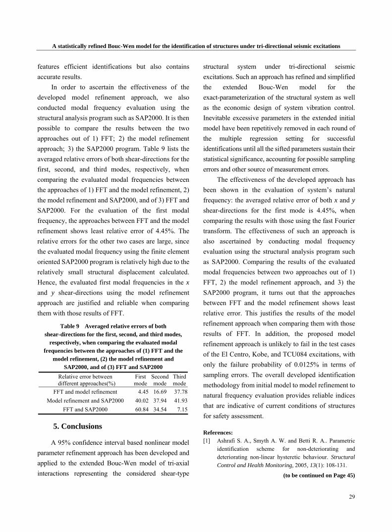
A statistically refined Bouc-Wen model for the identification of structures under tri-directional seismic excitations
29
features efficient identifications but also contains accurate results.
In order to ascertain the effectiveness of the developed model refinement approach, we also conducted modal frequency evaluation using the structural analysis program such as SAP2000. It is then possible to compare the results between the two approaches out of 1) FFT; 2) the model refinement approach; 3) the SAP2000 program. Table 9 lists the averaged relative errors of both shear-directions for the first, second, and third modes, respectively, when comparing the evaluated modal frequencies between the approaches of 1) FFT and the model refinement, 2) the model refinement and SAP2000, and of 3) FFT and SAP2000. For the evaluation of the first modal frequency, the approaches between FFT and the model refinement shows least relative error of 4.45%. The relative errors for the other two cases are large, since the evaluated modal frequency using the finite element oriented SAP2000 program is relatively high due to the relatively small structural displacement calculated. Hence, the evaluated first modal frequencies in the x and y shear-directions using the model refinement approach are justified and reliable when comparing them with those results of FFT.
Table 9 Averaged relative errors of both shear-directions for the first, second, and third modes,
respectively, when comparing the evaluated modal frequencies between the approaches of (1) FFT and the
model refinement, (2) the model refinement and SAP2000, and of (3) FFT and SAP2000
Relative error between different approaches(%)
First mode
Second mode
Third mode
FFT and model refinement 4.45 16.69 37.78Model refinement and SAP2000 40.02 37.94 41.93
FFT and SAP2000 60.84 34.54 7.15
5. Conclusions
A 95% confidence interval based nonlinear model parameter refinement approach has been developed and applied to the extended Bouc-Wen model of tri-axial interactions representing the considered shear-type
structural system under tri-directional seismic excitations. Such an approach has refined and simplified the extended Bouc-Wen model for the exact-parameterization of the structural system as well as the economic design of system vibration control. Inevitable excessive parameters in the extended initial model have been repetitively removed in each round of the multiple regression setting for successful identifications until all the sifted parameters sustain their statistical significance, accounting for possible sampling errors and other source of measurement errors.
The effectiveness of the developed approach has been shown in the evaluation of system’s natural frequency: the averaged relative error of both x and y shear-directions for the first mode is 4.45%, when comparing the results with those using the fast Fourier transform. The effectiveness of such an approach is also ascertained by conducting modal frequency evaluation using the structural analysis program such as SAP2000. Comparing the results of the evaluated modal frequencies between two approaches out of 1) FFT, 2) the model refinement approach, and 3) the SAP2000 program, it turns out that the approaches between FFT and the model refinement shows least relative error. This justifies the results of the model refinement approach when comparing them with those results of FFT. In addition, the proposed model refinement approach is unlikely to fail in the test cases of the El Centro, Kobe, and TCU084 excitations, with only the failure probability of 0.0125% in terms of sampling errors. The overall developed identification methodology from initial model to model refinement to natural frequency evaluation provides reliable indices that are indicative of current conditions of structures for safety assessment. References: [1] Ashrafi S. A., Smyth A. W. and Betti R. A.. Parametric
identification scheme for non-deteriorating and deteriorating non-linear hysteretic behaviour. Structural Control and Health Monitoring, 2005, 13(1): 108-131.
(to be continued on Page 45)
May 2009, Volume 3, No.5 (Serial No.18) Journal of Civil Engineering and Architecture, ISSN 1934-7359, USA
30
Tall building configuration effects on their response
to earthquake loading
Mohammed S. Al-Ansari (Civil and Architectural Engineering Department, Qatar University, Doha 2713, Qatar)
Abstract: This paper studies and analyzes the response and behavior of regular and irregular building structures in earthquake zones. The non-linear dynamic response of tall buildings structures were obtained using five simulated models, which were subjected to UBC code dynamic and static equivalent earthquake loads. The maximum response of the structural models were computed and analyzed in order to verify the effects of building configuration on drift results. Drift results agreed with codes recommendations regarding building configuration and showed that regular buildings performance in resisting earthquake forces is better than that of irregular buildings. Key words: drift; configuration; response; earthquake loads
1. Introduction
The response of tall building to earthquake loading depends on its configuration. Building configuration can be defined as building size and shape in a 3D form and recently there has been increased emphasis on the importance of a building’s configuration Fig. 1. Both shape and structural system work together to make the structure image distinctive or attractive and early decisions concerning size, shape, arrangement, and location of major building elements can have a significant effect on the building’s performance. Size and shape of the building establishes its mass that is the major determinant of the total inertial forces in the building[1].
Improper architectural -structural configuration is one of the greatest causes of damage to buildings because each of these choices of shapes and structure
Mohammed S. Al-Ansari, male, Ph.D., associate professor;
research fields: structure analysis and design, earthquake engineering. E-mail: [email protected].
has significant effects on the response of the building to earthquake loading. Interaction between architect and structural engineer is required as a designer must realize that a building’s configuration will determine were seismic damage will occur because earthquake forces will be concentrated in the areas of poor aspect and detailing causing maximum damage.
Architects play a key role in determining the form and function of buildings and balancing many conflicting factors. For this reason, the architect may have a more significant effect on the building’s earthquake performance than the structural engineer may, and both share the earthquake resistance building's design responsibility but structural engineer is held liable for building’s safety, stability and design quality[2-6].
Structure response as a building drift (roof displacement) is the key parameter in performance- based seismic design rather than force or strength that is used in conventional code design approaches because performance is characterized by the level of damage and damage is related to building displacement. This paper studies and analyzes the response of buildings with different configuration and material in earthquake zones. The building response to UBC static equivalent and dynamic earthquake loads was computed, documented, and analyzed using simulated computer models[7].
2. Out line of the numerical work
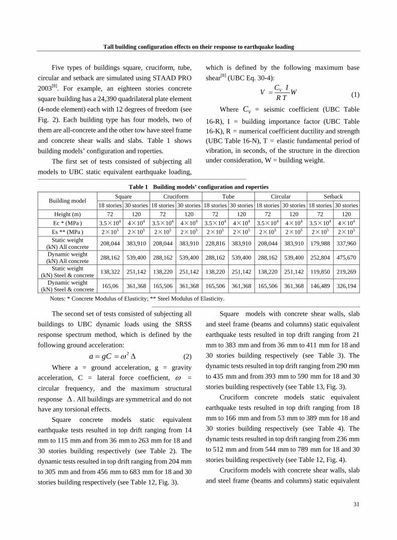
Tall building configuration effects on their response to earthquake loading
31
Five types of buildings square, cruciform, tube, circular and setback are simulated using STAAD PRO 2003[8]. For example, an eighteen stories concrete square building has a 24,390 quadrilateral plate element (4-node element) each with 12 degrees of freedom (see Fig. 2). Each building type has four models, two of them are all-concrete and the other tow have steel frame and concrete shear walls and slabs. Table 1 shows building models’ configuration and roperties.
The first set of tests consisted of subjecting all models to UBC static equivalent earthquake loading,
which is defined by the following maximum base shear[8] (UBC Eq. 30-4):
VC IV WR T
= (1)
Where VC = seismic coefficient (UBC Table
16-R), I = building importance factor (UBC Table 16-K), R = numerical coefficient ductility and strength (UBC Table 16-N), T = elastic fundamental period of vibration, in seconds, of the structure in the direction under consideration, W = building weight.
Table 1 Building models’ configuration and roperties Square Cruciform Tube Circular Setback
Building model 18 stories 30 stories 18 stories 30 stories 18 stories 30 stories 18 stories 30 stories 18 stories 30 stories
Height (m) 72 120 72 120 72 120 72 120 72 120 Ec * (MPa ) 3.5×10⁴ 4×10⁴ 3.5×10⁴ 4×10⁴ 3.5×10⁴ 4×10⁴ 3.5×10⁴ 4×10⁴ 3.5×10⁴ 4×10⁴
Es ** (MPa ) 2×10⁵ 2×10⁵ 2×10⁵ 2×10⁵ 2×10⁵ 2×10⁵ 2×10⁵ 2×10⁵ 2×10⁵ 2×10⁵
Static weight (kN) All concrete 208,044 383,910 208,044 383,910 228,816 383,910 208,044 383,910 179,988 337,960
Dynamic weight (kN) All concrete 288,162 539,400 288,162 539,400 288,162 539,400 288,162 539,400 252,804 475,670
Static weight (kN) Steel & concrete 138,322 251,142 138,220 251,142 138,220 251,142 138,220 251,142 119,850 219,269
Dynamic weight (kN) Steel & concrete 165,06 361,368 165,506 361,368 165,506 361,368 165,506 361,368 146,489 326,194
Notes: * Concrete Modulus of Elasticity; ** Steel Modulus of Elasticity.
The second set of tests consisted of subjecting all buildings to UBC dynamic loads using the SRSS response spectrum method, which is defined by the following ground acceleration:
2a gC ω= = Δ (2) Where a = ground acceleration, g = gravity
acceleration, C = lateral force coefficient, ω = circular frequency, and the maximum structural response Δ . All buildings are symmetrical and do not have any torsional effects.
Square concrete models static equivalent earthquake tests resulted in top drift ranging from 14 mm to 115 mm and from 36 mm to 263 mm for 18 and 30 stories building respectively (see Table 2). The dynamic tests resulted in top drift ranging from 204 mm to 305 mm and from 456 mm to 683 mm for 18 and 30 stories building respectively (see Table 12, Fig. 3).
Square models with concrete shear walls, slab and steel frame (beams and columns) static equivalent earthquake tests resulted in top drift ranging from 21 mm to 383 mm and from 36 mm to 411 mm for 18 and 30 stories building respectively (see Table 3). The dynamic tests resulted in top drift ranging from 290 mm to 435 mm and from 393 mm to 590 mm for 18 and 30 stories building respectively (see Table 13, Fig. 3).
Cruciform concrete models static equivalent earthquake tests resulted in top drift ranging from 18 mm to 166 mm and from 53 mm to 389 mm for 18 and 30 stories building respectively (see Table 4). The dynamic tests resulted in top drift ranging from 236 mm to 512 mm and from 544 mm to 789 mm for 18 and 30 stories building respectively (see Table 12, Fig. 4).
Cruciform models with concrete shear walls, slab and steel frame (beams and columns) static equivalent
Tall building configuration effects on their response to earthquake loading
32
earthquake tests resulted in top drift ranging from 29 mm to 468 mm and from 47 mm to 598 mm for 18 and 30 storyies building respectively (see Table 5). The dynamic tests resulted in top drift ranging from 316 mm to 473 mm and from 488 mm to 732 mm for 18 and 30 stories building respectively (see Table 13, Fig. 4).
Tube buildings concrete models static equivalent earthquake tests resulted in top drift ranging from 18 mm to 131 mm and from 46 mm to 329 mm for 18 and 30 stories building respectively (see Table 6). The dynamic tests resulted in top drift ranging from 326 mm to 489 mm and from 525 mm to 789 for 18 and 30 stories building respectively (see Table 12, Fig. 5).
Tube buildings models with concrete shear walls, slab and steel frame (beams and columns) static equivalent earthquake tests resulted in top drift ranging from 31 mm to 495 mm and from 46 mm to 574 mm for 18 and 30 stories building respectively (see Table 7). The dynamic tests resulted in top drift ranging from 351 mm to 526 mm and from 454 mm to 681 mm for 18 and 30 stories building respectively (see Table 13, Fig. 5).
Circular buildings concrete models static equivalent earthquake tests resulted in top drift ranging from 17 mm to 127 mm and from 41 mm to 290 mm for 18 and 30 stories building respectively (see Table 8). The dynamic tests resulted in top drift ranging from 223 mm to 334 mm and from 505 mm to 758 mm for 18 and 30 stories building respectively (see Table 12, Fig. 6).
Circular Buildings models with concrete shear walls, slab and steel frame (beams and columns) static equivalent earthquake tests resulted in top drift ranging from 20 mm to 381 mm and from 42 mm to 485 mm for 18 and 30 stories building respectively (see Table 9). The dynamic tests resulted in top drift ranging from 302 mm to 452 mm and from 431 mm to 647 mm for 18 and 30 stories building respectively (see Table 13, Fig. 6).
Setback buildings concrete models static equivalent earthquake tests resulted in top drift ranging
from 12 mm to 115 mm and from 31 mm to 228 for 18 and 30 stories building respectively (see Table 10). The dynamic tests resulted in top drift ranging from 187 mm to 279 mm and from 418 mm to 627 mm for 18 and 30 stories building respectively (see Table 12, Fig. 7).
Setback buildings models with concrete shear walls, slab and steel frame (beams and columns) static equivalent earthquake tests resulted in top drift ranging from 18 mm to 289 mm and from 31 mm to 384 mm for 18 and 30 stories building respectively (see Table 11). The dynamic tests resulted in top drift ranging from 268 mm to 401 mm and from 362 mm to 542 mm for 18 and 30 stories building respectively (see Table 13, Fig. 7).
3. Results and discussion
Concrete building models drifts of 18 stories subjected to static equivalent earthquake loads showed that the square model performed the best with the least drift in all earthquake zones. Zone 4 was chosen as an example. It is worth mentioning that the setback model in zone 4 has a smaller drift (114.5 mm) than the square model (115.5 mm) because of its lighter weight. For a setback model having the same weight as the square model, the setback model drift (221 mm) is higher than the square model drift.
The 18 stories building models with steel frames response to static equivalent earthquake loads was very close in its general behavior to that of total concrete building models. Zone 3 was chosen as an example (see Fig. 8).
Concrete building models drifts of 30 stories subjected to static equivalent earthquake loads showed that the square model performed the best with the least drift in all earthquake zones. Zone 2 was chosen as an example (see Fig. 9). It is worth mentioning that the 18 stories cruciform model has a very close drift to that of the tube model, but the 30 stories cruciform model has a larger drift than that of 30 stories tube model and it

Tall building configuration effects on their response to earthquake loading
33
gets larger with the increase of the earthquake loads and soil profile.
The 30 stories building models with steel frames response to static equivalent earthquake loads was very close in its general behavior to that of total concrete building models. Zone 1 was chosen as an example (see Fig. 10).
Concrete building models drifts of 18 and 30 stories subjected to dynamic earthquake loads showed that the square model performed the best with the least drift in all earthquake zones (see Fig. 11). The 18 and 30 stories building models with steel frames response to dynamic earthquake loads was very close in its general behavior to that of total concrete building models (see Fig. 12).
Table 2 Concrete square building response to equivalent static load
xΔ (mm) Zone 18 stories 30 stories
soil type
1 14.322 35.966 S1 19.084 47.943 S2 21.465 53.931 S3 28.608 71.896 S4 45.282 113.815 S5
2 28.608 71.896 S1 35.754 89.861 S2 42.900 107.827 S3 52.429 131.781 S4 71.485 179.689 S5
3 38.136 95.85 S1 47.664 119.804 S2 57.193 143.758 S3 66.721 167.712 S4 81.014 203.645 S5
4 57.193 143.758 S1 71.485 179.689 S2 78.632 197.665 S3 85.778 215.624 S4 101.403 215.624 S5
5 81.549 204.990 S1 95.307 239.582 S2 95.307 239.582 S3 104.835 263.54 S4 115.475 263.54 S5
Table 3 Steel frame square building response to equivalent static load
xΔ (mm) Zone 18 stories 30 stories
soil type
1 20.502 35.606 S1 27.328 47.466 S2 38.754 53.396 S3 53.654 72.241 S4 77.496 112.695 S5
2 40.98 71.185 S1 51.222 88.975 S2 74.516 106.765 S3 95.38 130.484 S4 149.031 200.622 S5
3 54.636 94.905 S1 68.292 118.624 S2 95.38 142.344 S3 119.225 166.064 S4 190.760 256.789 S5
4 81.950 142.344 S1 102.437 177.923 S2 134.128 195.713 S3 160.954 216.670 S4 250.372 337.032 S5
5 230.608 410.767 S1 230.608 410.767 S2 230.608 410.767 S3 255.612 410.767 S4 383.419 410.767 S5
Table 4 Concrete cruciform building response
to equivalent static load
xΔ (mm) Zone 18 stories 30 stories
soil type
1 17.982 53.158 S1 23.967 70.861 S2 26.959 79.712 S3 35.935 106.267 S4 56.887 168.228 S5 2 35.935 106.267 S1 44.915 132.822 S2 53.849 159.377 S3 65.867 194.783 S4 89.812 265.605 S5 3 47.908 141.673 S1 59.880 177.080 S2 71.853 212.486 S3 83.825 247.898 S4 101.784 301.018 S5
(to be continued)

Tall building configuration effects on their response to earthquake loading
34
4 71.853 212.486 S1 89.812 265.605 S2 98.791 292.195 S3 107.711 318.725 S4 114.272 318.725 S5
5 100.426 303.007 S1 117.370 354.139 S2 117.370 354.139 S3 129.107 389.553 S4 166.696 389.553 S5
Table 5 Steel frame cruciform building response to equivalent static load
xΔ (mm) Zone 18 stories 30 stories
soil type
1 29.251 47.362 S1 38.993 63.138 S2 66.459 71.026 S3 92.010 94.689 S4 132.894 149.905 S5 2 61.348 94.689 S1 73.099 118.353 S2 121.829 142.017 S3 155.941 173.569 S4 243.657 236.672 S5 3 77.971 126.241 S1 97.463 157.793 S2 155.941 189.344 S3 194.926 220.896 S4 311.881 302.896 S5 4 116.955 189.344 S1 146.194 236.672 S2 219.291 260.336 S3 263.150 283.999 S4 409.344 397.545 S5 5 281.372 527.275 S1 281.372 527.275 S2 281.372 527.275 S3 311.881 527.275 S4 467.822 597.654 S5
Table 6 Concrete tube building response to equivalent static load
xΔ (mm) Zone 18 stories 30 stories
soil type
1 18.146 46.488 S1 24.124 61.947 S2 27.113 69.677 S3 36.080 92.867 S4 57.003 146.976 S5 2 36.080 92.867 S1 45.047 116.057 S2
54.014 139.247 S3 65.970 170.166 S4 89.882 232.005 S5
3 48.036 123.787 S1 59.992 154.706 S2 71.948 185.625 S3 83.904 216.546 S4 101.838 262.925 S5
4 71.948 185.625 S1 89.882 232.005 S2 98.849 255.195 S3 107.816 278.385 S4 114.846 278.385 S5
5 102.510 256.053 S1 119.772 299.249 S2 119.772 299.249 S3 131.728 329.163 S4 131.223 329.163 S5
Table 7 Steel frametube building response to equivalent satic load
xΔ (mm) Zone 18 stories 30 stories
Soil type
1 30.959 45.734 S1 41.258 60.867 S2 67.024 68.434 S3 92.802 91.133 S4 134.048 144.099 S5 2 61.868 91.133 S1 77.335 113.833 S2 128.892 136.532 S3 164.982 166.798 S4 257.785 230.822 S5 3 82.491 121.399 S1 103.114 151.665 S2 164.982 181.931 S3 206.228 212.197 S4 329.965 295.359 S5 4 123.737 181.931 S1 154.671 227.330 S2 232.006 250.029 S3 278.408 272.729 S4 433.078 387.553 S5 5 297.687 506.578 S1 267.687 506.578 S2 297.687 506.578 S3 329.965 506.578 S4 494.947 574.149 S5
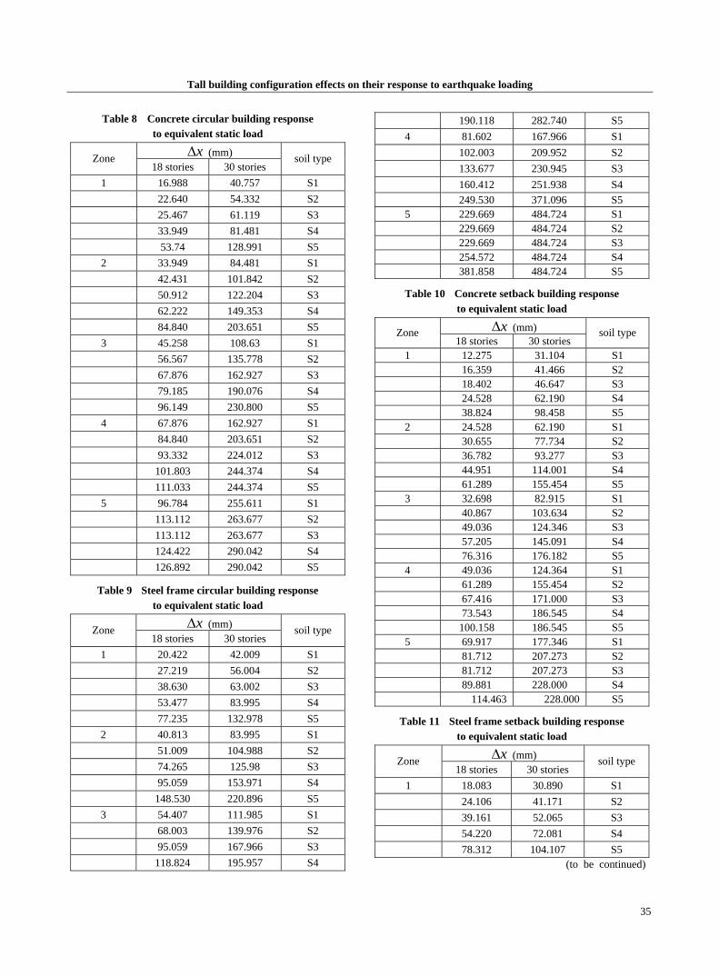
Tall building configuration effects on their response to earthquake loading
35
Table 8 Concrete circular building response to equivalent static load
xΔ (mm) Zone 18 stories 30 stories
soil type
1 16.988 40.757 S1 22.640 54.332 S2 25.467 61.119 S3 33.949 81.481 S4 53.74 128.991 S5 2 33.949 84.481 S1 42.431 101.842 S2 50.912 122.204 S3 62.222 149.353 S4 84.840 203.651 S5 3 45.258 108.63 S1 56.567 135.778 S2 67.876 162.927 S3 79.185 190.076 S4 96.149 230.800 S5 4 67.876 162.927 S1 84.840 203.651 S2 93.332 224.012 S3 101.803 244.374 S4 111.033 244.374 S5 5 96.784 255.611 S1 113.112 263.677 S2 113.112 263.677 S3 124.422 290.042 S4 126.892 290.042 S5
Table 9 Steel frame circular building response
to equivalent static load
xΔ (mm) Zone 18 stories 30 stories
soil type
1 20.422 42.009 S1 27.219 56.004 S2 38.630 63.002 S3 53.477 83.995 S4 77.235 132.978 S5
2 40.813 83.995 S1 51.009 104.988 S2 74.265 125.98 S3 95.059 153.971 S4 148.530 220.896 S5
3 54.407 111.985 S1 68.003 139.976 S2 95.059 167.966 S3 118.824 195.957 S4
190.118 282.740 S5 4 81.602 167.966 S1 102.003 209.952 S2 133.677 230.945 S3 160.412 251.938 S4 249.530 371.096 S5
5 229.669 484.724 S1 229.669 484.724 S2 229.669 484.724 S3 254.572 484.724 S4 381.858 484.724 S5
Table 10 Concrete setback building response
to equivalent static load
xΔ (mm) Zone 18 stories 30 stories
soil type
1 12.275 31.104 S1 16.359 41.466 S2 18.402 46.647 S3 24.528 62.190 S4 38.824 98.458 S5 2 24.528 62.190 S1 30.655 77.734 S2 36.782 93.277 S3 44.951 114.001 S4 61.289 155.454 S5 3 32.698 82.915 S1 40.867 103.634 S2 49.036 124.346 S3 57.205 145.091 S4 76.316 176.182 S5 4 49.036 124.364 S1 61.289 155.454 S2 67.416 171.000 S3 73.543 186.545 S4 100.158 186.545 S5 5 69.917 177.346 S1 81.712 207.273 S2 81.712 207.273 S3 89.881 228.000 S4 114.463 228.000 S5
Table 11 Steel frame setback building response
to equivalent static load
xΔ (mm) Zone 18 stories 30 stories
soil type
1 18.083 30.890 S1 24.106 41.171 S2 39.161 52.065 S3 54.220 72.081 S4 78.312 104.107 S5
(to be continued)
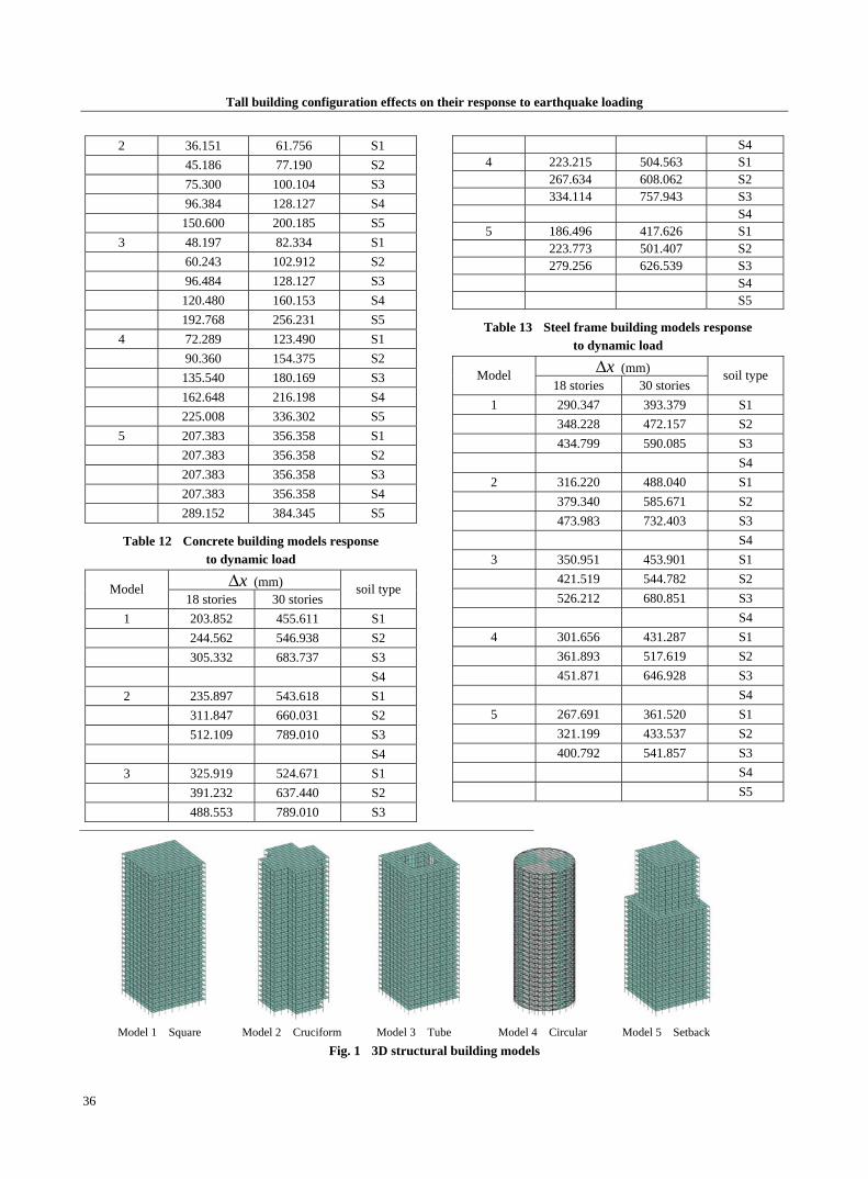
Tall building configuration effects on their response to earthquake loading
36
2 36.151 61.756 S1 45.186 77.190 S2 75.300 100.104 S3 96.384 128.127 S4 150.600 200.185 S5
3 48.197 82.334 S1 60.243 102.912 S2 96.484 128.127 S3 120.480 160.153 S4 192.768 256.231 S5
4 72.289 123.490 S1 90.360 154.375 S2 135.540 180.169 S3 162.648 216.198 S4 225.008 336.302 S5
5 207.383 356.358 S1 207.383 356.358 S2 207.383 356.358 S3 207.383 356.358 S4 289.152 384.345 S5
Table 12 Concrete building models response
to dynamic load
xΔ (mm) Model 18 stories 30 stories
soil type
1 203.852 455.611 S1 244.562 546.938 S2 305.332 683.737 S3 S4 2 235.897 543.618 S1 311.847 660.031 S2 512.109 789.010 S3 S4 3 325.919 524.671 S1 391.232 637.440 S2 488.553 789.010 S3
S4 4 223.215 504.563 S1 267.634 608.062 S2 334.114 757.943 S3 S4
5 186.496 417.626 S1 223.773 501.407 S2 279.256 626.539 S3 S4 S5
Table 13 Steel frame building models response
to dynamic load
xΔ (mm) Model 18 stories 30 stories
soil type
1 290.347 393.379 S1 348.228 472.157 S2 434.799 590.085 S3 S4 2 316.220 488.040 S1 379.340 585.671 S2 473.983 732.403 S3 S4 3 350.951 453.901 S1 421.519 544.782 S2 526.212 680.851 S3 S4 4 301.656 431.287 S1 361.893 517.619 S2 451.871 646.928 S3 S4 5 267.691 361.520 S1 321.199 433.537 S2 400.792 541.857 S3 S4 S5
Model 1 Square Model 2 Cruciform Model 3 Tube Model 4 Circular Model 5 Setback Fig. 1 3D structural building models
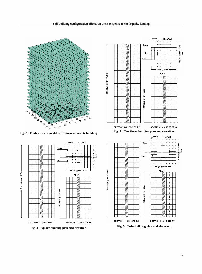
Tall building configuration effects on their response to earthquake loading
37
Fig. 2 Finite element model of 18 stories concrete building
Fig. 3 Square building plan and elevation
Fig. 4 Cruciform building plan and elevation
Fig. 5 Tube building plan and elevation
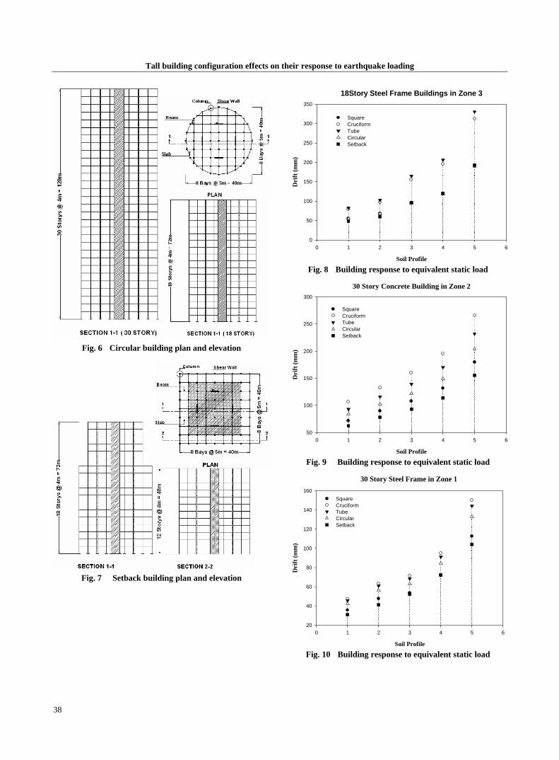
Tall building configuration effects on their response to earthquake loading
38
Fig. 6 Circular building plan and elevation
Fig. 7 Setback building plan and elevation
18Story Steel Frame Buildings in Zone 3
Soil Profile
0 1 2 3 4 5 6
Dri
ft (m
m)
0
50
100
150
200
250
300
350
SquareCruciformTubeCircularSetback
Fig. 8 Building response to equivalent static load
30 Story Concrete Building in Zone 2
Soil Profile
0 1 2 3 4 5 6
Dri
ft (m
m)
50
100
150
200
250
300
SquareCruciformTubeCircularSetback
Fig. 9 Building response to equivalent static load
30 Story Steel Frame in Zone 1
Soil Profile
0 1 2 3 4 5 6
Dri
ft (m
m)
20
40
60
80
100
120
140
160SquareCruciformTubeCircularSetback
Fig. 10 Building response to equivalent static load
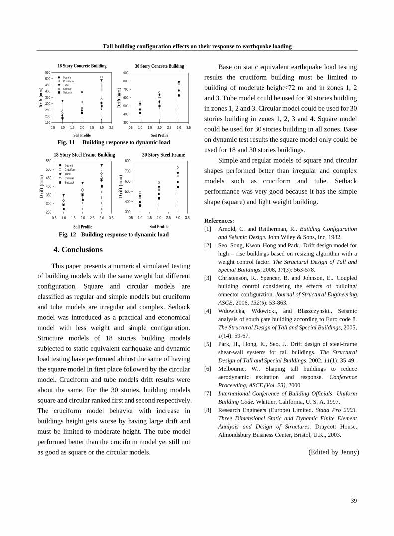
Tall building configuration effects on their response to earthquake loading
39
18 Story Concrete Building 30 Story Concrete Building
Soil Profile
0.5 1.0 1.5 2.0 2.5 3.0 3.5
Dri
ft (m
m)
150
200
250
300
350
400
450
500
550SquareCruciformTubeCircularSetback
Soil Profile
0.5 1.0 1.5 2.0 2.5 3.0 3.5
Dri
ft (m
m)
300
400
500
600
700
800
900
Fig. 11 Building response to dynamic load
18 Story Steel Frame Building 30 Story Steel Frame
Soil Profile
0.5 1.0 1.5 2.0 2.5 3.0 3.5
Dri
ft (m
m)
250
300
350
400
450
500
550SquareCruciformTubeCircularSetback
Soil Profile
0.5 1.0 1.5 2.0 2.5 3.0 3.5
Dri
ft (m
m)
300
400
500
600
700
800
Fig. 12 Building response to dynamic load
4. Conclusions
This paper presents a numerical simulated testing of building models with the same weight but different configuration. Square and circular models are classified as regular and simple models but cruciform and tube models are irregular and complex. Setback model was introduced as a practical and economical model with less weight and simple configuration. Structure models of 18 stories building models subjected to static equivalent earthquake and dynamic load testing have performed almost the same of having the square model in first place followed by the circular model. Cruciform and tube models drift results were about the same. For the 30 stories, building models square and circular ranked first and second respectively. The cruciform model behavior with increase in buildings height gets worse by having large drift and must be limited to moderate height. The tube model performed better than the cruciform model yet still not as good as square or the circular models.
Base on static equivalent earthquake load testing results the cruciform building must be limited to building of moderate height<72 m and in zones 1, 2 and 3. Tube model could be used for 30 stories building in zones 1, 2 and 3. Circular model could be used for 30 stories building in zones 1, 2, 3 and 4. Square model could be used for 30 stories building in all zones. Base on dynamic test results the square model only could be used for 18 and 30 stories buildings.
Simple and regular models of square and circular shapes performed better than irregular and complex models such as cruciform and tube. Setback performance was very good because it has the simple shape (square) and light weight building.
References: [1] Arnold, C. and Reitherman, R.. Building Configuration
and Seismic Design. John Wiley & Sons, Inc, 1982. [2] Seo, Song, Kwon, Hong and Park.. Drift design model for
high – rise buildings based on resizing algorithm with a weight control factor. The Structural Design of Tall and Special Buildings, 2008, 17(3): 563-578.
[3] Christenson, R., Spencer, B. and Johnson, E.. Coupled building control considering the effects of building/ onnector configuration. Journal of Structural Engineering, ASCE, 2006, 132(6): 53-863.
[4] Wdowicka, Wdowicki, and Blaszczynski.. Seismic analysis of south gate building according to Euro code 8. The Structural Design of Tall and Special Buildings, 2005, 1(14): 59-67.
[5] Park, H., Hong, K., Seo, J.. Drift design of steel-frame shear-wall systems for tall buildings. The Structural Design of Tall and Special Buildings, 2002, 11(1): 35-49.
[6] Melbourne, W.. Shaping tall buildings to reduce aerodynamic excitation and response. Conference Proceeding, ASCE (Vol. 23), 2000.
[7] International Conference of Building Officials: Uniform Building Code. Whittier, California, U. S. A. 1997.
[8] Research Engineers (Europe) Limited. Staad Pro 2003. Three Dimensional Static and Dynamic Finite Element Analysis and Design of Structures. Draycott House, Almondsbury Business Center, Bristol, U.K., 2003.
(Edited by Jenny)

May 2009, Volume 3, No.5 (Serial No.18) Journal of Civil Engineering and Architecture, ISSN 1934-7359, USA
40
Experimental analysis of Tuned Liquid Damper (TLD)
for high raised structures
S. Arash Sohrabi, Samad Dehghan (Islamic Council of East Azerbaijan Province-Consultant, Iranian National Retrofitting Center-north West Branch)
Abstract: Tuned liquid damper is one the passive structural control ways which has been used since mid 1980 decade for seismic control in civil engineering. This system is made of one or many tanks filled with fluid, mostly water that installed on top of the high raised structure and used to prevent structure vibration. In this article we will show how to make seismic table contain TLD system and analysis the result of using this system in our structure. Results imply that when frequency ratio approaches 1 this system can perform its best in both dissipate energy and increasing structural damping. And also results of these serial experiments are proved compatible with Hunzer linear theory behavior. Key words: TLD; seismic table; structural system; Hunzer linear behavior
1. Introduction
Nowadays using methods for absorbing energy of earthquake, wind and etc. including designing resistant buildings, specially in the case of already built structure retrofitting, are popular amongst engineers in a way that with adding some equipments and systems to the structure, it’s possible to reduce the energy level influencing the structure, so that structure responses and destructions of structure will be decreased tremendously. For this purpose using new technologies in the damper field is essential.
High raised buildings are often under strong dynamic loads caused by the environmental factors including loads caused by earthquakes, strong winds and etc., that’s why the biggest obstacle for the structural engineers is to find ways to lessen the
Corresponding author: S. Arash Sohrabi, professor;
research field: seismic retrofitting. E-mail: [email protected], [email protected].
structure’s lateral motions and vibrations caused in the high raised structure to increase safety factor. Nowadays most of the high raised buildings are built using different motion controlling tools that are mostly passive-based, e.g. Viscoelastic dampers (VED), Tuned mass dampers (TMD), Friction dampers (FD), Stainless steel dampers (SSD) and Tuned Liquid Dampers (TLD) that is used in very countries, for example Fukuoka Tower in Japan.
2. Liquid damper theory
Since water sloshing properties are non-linear, it’s not a good idea to analyze it using potential theory, but in the case of deep water tanks that are open to small excitations, velocity of sloshing can be analyzed by the potential theory.
In the following experiments, TLD tank is considered as a rigid body. In a tank with the length of L and the depth of H that is shown in Fig 1. X and Y axes are considered as the horizontal and vertical axes, the water in the tank is considered as ideal, incompressible, nonviscous, and irrotational. η is considered as vertical movement of the water surface of the tank that all of the above mentioned unknown factors can be calculated:
tLx
gC
tg Hy
ωπωφη sincos21 1=⎟
⎠⎞
⎜⎝⎛
∂∂
==
(1)
( )[ ]( ) t
Lx
LHLHy
gC
tx ωπ
πππφ coscos
/cosh/cosh2 1 +
−=∂∂
= (2)
( )[ ]( ) t
Lx
LHLHy
gC
ty ωπ
πππφ coscos
/cosh/sinh2 1 +
=∂∂
= (3)

Experimental analysis of Tuned Liquid Damper (TLD) for high raised structures
41
In above equations, g stands for gravity
acceleration, φ is considered as the potential energy function, t stands for time, C stands for const., ω is considered as angle velocity (radian per second), also the velocity is distributed horizontally and vertically based on the equations No. 2 and No. 3 as shown in the Fig. 2.
Fig. 1 View of wave surface inside the tank
Fig. 2 Velocity distribution in the tank
Horizontal velocity in the tank’s center is in its maximum and with approaching to the sides, it will decrease; vertical velocity in bottom of the tank is zero and on the sides are in its maximum. In order to increase damping effect, one can use the bumps on the sides of the tank, where the vertical velocity is in its maximum. Of course in this paper’s experiments, horizontal velocity is considered as the main cause of
the damping of the TLD system and to increase the damping effect of water sloshing fender screens is used in the center of the tank, where the horizontal velocity is in its maximum, and placed vertically on the tank. Fig. 3 is showing the tank and metal drilled screens that is used in the experiment. As shown in the picture, screens are placed, in equal distance of 22 cm from the end, in the prepared tracks on the tank. To prevent the sides of the glass tank from breaking down in the time of seismic table experiment, vulcanite, with the thickness of 5 cm , is placed on the sides. Length of the tank is about 70 cm with height of about 32 cm and width of about 35 cm.
Fig. 3 Schematic and TLD system tank view
Connection between equal damping factor (ξeq) and excitement domain ratio (D/L) is shown in the Table 1 calculated using equation No. 4 for the cases of no screen, one screen and two screens. Equal damping factor is connected directly to the numbers of fender screens and it has no connections to the shape factor. With increasing the number of fender screens, equal damping factor increases, so damping factor of fender
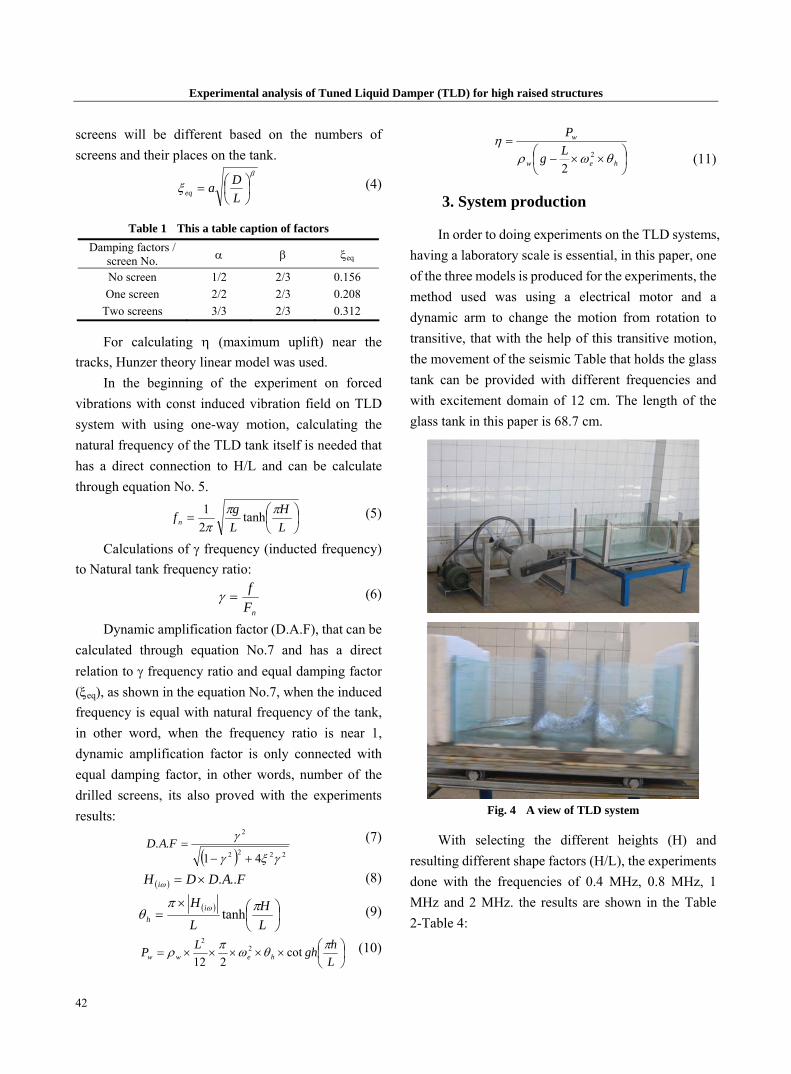
Experimental analysis of Tuned Liquid Damper (TLD) for high raised structures
42
screens will be different based on the numbers of screens and their places on the tank.
β
ξ ⎟⎠⎞
⎜⎝⎛=
LDaeq
(4)
Table 1 This a table caption of factors Damping factors /
screen No. α β ξeq
No screen 1/2 2/3 0.156 One screen 2/2 2/3 0.208
Two screens 3/3 2/3 0.312
For calculating η (maximum uplift) near the tracks, Hunzer theory linear model was used.
In the beginning of the experiment on forced vibrations with const induced vibration field on TLD system with using one-way motion, calculating the natural frequency of the TLD tank itself is needed that has a direct connection to H/L and can be calculate through equation No. 5.
⎟⎠⎞
⎜⎝⎛=
LH
Lgfn
πππ
tanh21 (5)
Calculations of γ frequency (inducted frequency) to Natural tank frequency ratio:
nFf
=γ (6)
Dynamic amplification factor (D.A.F), that can be calculated through equation No.7 and has a direct relation to γ frequency ratio and equal damping factor (ξeq), as shown in the equation No.7, when the induced frequency is equal with natural frequency of the tank, in other word, when the frequency ratio is near 1, dynamic amplification factor is only connected with equal damping factor, in other words, number of the drilled screens, its also proved with the experiments results:
( ) 2222
2
41..
γξγ
γ
+−=FAD (7)
( ) FADDH i ...×=ω (8)
( )⎟⎠⎞
⎜⎝⎛×
=LH
L
H ih
ππθ ω tanh (9)
⎟⎠⎞
⎜⎝⎛×××××=
LhghLP heww
πθωπρ cot212
22
(10)
⎟⎠⎞
⎜⎝⎛ ××−
=
hew
w
Lg
P
θωρη
2
2
(11)
3. System production
In order to doing experiments on the TLD systems, having a laboratory scale is essential, in this paper, one of the three models is produced for the experiments, the method used was using a electrical motor and a dynamic arm to change the motion from rotation to transitive, that with the help of this transitive motion, the movement of the seismic Table that holds the glass tank can be provided with different frequencies and with excitement domain of 12 cm. The length of the glass tank in this paper is 68.7 cm.
Fig. 4 A view of TLD system
With selecting the different heights (H) and resulting different shape factors (H/L), the experiments done with the frequencies of 0.4 MHz, 0.8 MHz, 1 MHz and 2 MHz. the results are shown in the Table 2-Table 4:
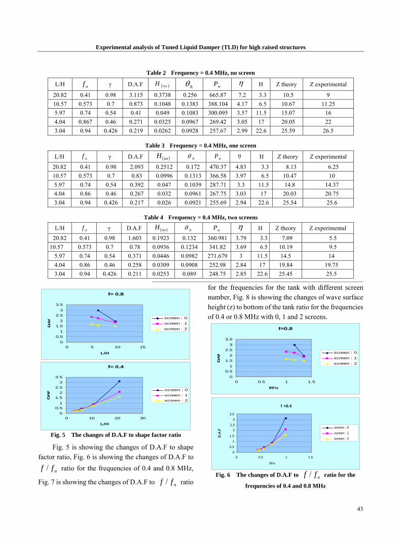
Experimental analysis of Tuned Liquid Damper (TLD) for high raised structures
43
Table 2 Frequency = 0.4 MHz, no screen
L/H nf γ D.A.F ( )ωiH hθ wP η H Z theory Z experimental
20.82 0.41 0.98 3.115 0.3738 0.256 665.87 7.2 3.3 10.5 9 10.57 0.573 0.7 0.873 0.1048 0.1383 388.104 4.17 6.5 10.67 11.25 5.97 0.74 0.54 0.41 0.049 0.1083 300.095 3.57 11.5 15.07 16 4.04 0.867 0.46 0.271 0.0325 0.0967 269.42 3.05 17 20.05 22 3.04 0.94 0.426 0.219 0.0262 0.0928 257.67 2.99 22.6 25.59 26.5
Table 3 Frequency = 0.4 MHz, one screen
L/H nf γ D.A.F ( )ωiH hθ wP η H Z theory Z experimental
20.82 0.41 0.98 2.093 0.2512 0.172 470.37 4.83 3.3 8.13 6.25 10.57 0.573 0.7 0.83 0.0996 0.1313 366.58 3.97 6.5 10.47 10 5.97 0.74 0.54 0.392 0.047 0.1039 287.71 3.3 11.5 14.8 14.37 4.04 0.86 0.46 0.267 0.032 0.0961 267.75 3.03 17 20.03 20.75 3.04 0.94 0.426 0.217 0.026 0.0921 255.69 2.94 22.6 25.54 25.6
Table 4 Frequency = 0.4 MHz, two screens
L/H nf γ D.A.F ( )ωiH hθ
wP η H Z theory Z experimental
20.82 0.41 0.98 1.603 0.1923 0.132 360.981 3.79 3.3 7.09 5.5 10.57 0.573 0.7 0.78 0.0936 0.1234 341.82 3.69 6.5 10.19 9.5
5.97 0.74 0.54 0.371 0.0446 0.0982 271.679 3 11.5 14.5 14 4.04 0.86 0.46 0.258 0.0309 0.0908 252.98 2.84 17 19.84 19.75 3.04 0.94 0.426 0.211 0.0253 0.089 248.75 2.85 22.6 25.45 25.5
f= 0.8
00.5
11.5
22.5
33.5
0 5 10 15
L/H
D.A
.f
screen : 0screen : 1screen : 2
f= 0.4
00.5
11.5
22.5
33.5
0 10 20 30
L/H
D.A.
F screen : 0screen : 1screen : 2
Fig. 5 The changes of D.A.F to shape factor ratio
Fig. 5 is showing the changes of D.A.F to shape factor ratio, Fig. 6 is showing the changes of D.A.F to
nff / ratio for the frequencies of 0.4 and 0.8 MHz,
Fig. 7 is showing the changes of D.A.F to nff / ratio
for the frequencies for the tank with different screen number, Fig. 8 is showing the changes of wave surface height (z) to bottom of the tank ratio for the frequencies of 0.4 or 0.8 MHz with 0, 1 and 2 screens.
f=0.8
00.5
11.5
22.5
33.5
0 0.5 1 1.5
f/Fn
D.A.
F screen : 0screen : 1screen : 2
Fig. 6 The changes of D.A.F to nff / ratio for the
frequencies of 0.4 and 0.8 MHz
f =0.4
0
1
2
3
0 0.5 1 1.5
f/Fn
D.A
.F screen : 0
screen : 1screen : 2
0.5
1.5
2.5
3.5
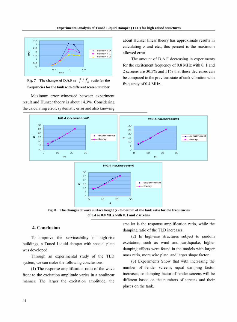
Experimental analysis of Tuned Liquid Damper (TLD) for high raised structures
44
0
0.5
1
1.5
2
2.5
3
3.5
0 0.5 1 1.5
f/Fn
D.A
.F
screen : 0screen : 1screen : 2
Fig. 7 The changes of D.A.F to nff / ratio for the
frequencies for the tank with different screen number
Maximum error witnessed between experiment result and Hunzer theory is about 14.3%. Considering the calculating error, systematic error and also knowing
about Hunzer linear theory has approximate results in calculating z and etc., this percent is the maximum allowed error.
The amount of D.A.F decreasing in experiments for the excitement frequency of 0.8 MHz with 0, 1 and 2 screens are 30.5% and 51% that these decreases can be compared to the previous state of tank vibration with frequency of 0.4 MHz.
f=0.4 no.screen=2
0
5
10
15
20
25
30
0 10 20 30
H
Z
experimentaltheory
f=0.4 no.screen=1
0
5
10
15
20
25
30
0 10 20 30
H
Z
exprrimentaltheory
f=0.4 no.screen=0
0
5
10
15
20
25
30
0 10 20 30
H
Z
experimentaltheory
Fig. 8 The changes of wave surface height (z) to bottom of the tank ratio for the frequencies
of 0.4 or 0.8 MHz with 0, 1 and 2 screens
4. Conclusion
To improve the serviceability of high-rise buildings, a Tuned Liquid damper with special plate was developed.
Through an experimental study of the TLD system, we can make the following conclusions.
(1) The response amplification ratio of the wave front to the excitation amplitude varies in a nonlinear manner. The larger the excitation amplitude, the
smaller is the response amplification ratio, while the damping ratio of the TLD increases.
(2) In high-rise structures subject to random excitation, such as wind and earthquake, higher damping effects were found in the models with larger mass ratio, more wire plate, and larger shape factor.
(3) Experiments Show that with increasing the number of fender screens, equal damping factor increases, so damping factor of fender screens will be different based on the numbers of screens and their places on the tank.
Experimental analysis of Tuned Liquid Damper (TLD) for high raised structures
45
(4) The amount of D.A.F decreasing in experiments for the excitement frequency of 0.8 MHz with 0, 1 and 2 screens are 30.5% and 51% that these decreases can be compared to the previous state of tank vibration with frequency of 0.4 MHz.
(5) The TLD shows good structural performance in reducing the vibration response of the structure. Therefore, it can be used as an efficient vibration control device for the tall buildings.
References: [1] Chopra, A. K.. Dynamic of structure: Theory and
Application to Earthquake Engineering Prentice Hall, Englewood Cliffs, N. J., 1995.
[2] Daewoo Institute of Construction Technology. The Design and Analysis of Tall Buildings. Technical Report, 1996, DEP-007-96.
[3] Young-Kyu Ju. Structural Behavior of Water Sloshing Damper with Embossments Subject to Random Excitation 2004, 31: 120-132.
[4] LI S. J., LI G. Q., TANG J. and LI Q. S.. Shallow cylindrical tuned liquid damper for vibration control of high-rise structures. The Structural Design of Tall Buildings, 2002, 11(4): 295-308.
[5] Reed, D., YU J. K., Yeh, H. and Gardarsson, S.. Investigation of tuned liquid dampers under large amplitude excitation. ASCE Journal of Engineering Mechanics, 1998, 124(4): 405-413.
[6] M. j. Tait, A. A. El Damatty, N. Isyumov, M. R.. Siddique numerical flow models to simulate Tuned Liquid Dampers (TLD) with slat screens. Journal of Fluids and Structures, 2005, 20: 007-1023.
[7] Emami Azadi and Moan T. Ductility demand analysis of simplification pile-soil-jacket system under extreme sea waves and earthquakes. Proc of EURODYN 96 Conf., 1996: 1025-1034.
(Edited by Jenny)
(continued from Page 29)
[2] Beck J. L and Jennings P. C.. Structural identification using linear models and earthquake records. Earthquake Engineering and Structural Dynamics, 1980, 8: 145-160.
[3] Lus H., Betti R. and Longman R. W.. Identification of linear structural systems using earthquake-induced vibration data. Earthquake Engineering and Structural Dynamics, 1999, 28: 1449-1467.
[4] LIN J. W., Betti R., Smyth A. W. and Longman R. W.. On-line identification of nonlinear hysteretic structural systems using a variable trace approach. Earthquake Engineering and Structural Dynamics, 2001, 30(9): 1279-1303.
[5] Longman R. W.. Notes on the health monitoring, Department of Mechanical Engineering. Columbia University, New York, 2002.
[6] LIN J W.. Adaptive algorithms for the identification of nonlinear structural systems, Doctoral dissertation, Columbia University, New York, 2001.
[7] YANG J N and LIN S.. Identification of parametric variations of structures based on least squares estimation and adaptive tracking technique. Journal of Engineering Mechanics ASCE, 2005, 131(3): 290-298.
[8] HUANG N. E., SHEN Z., LONG S. R., WU M. C., SHI H. H., ZHENG. Q., YEN N. C., TUNG C. C. and LIU H. H.. The empirical mode decomposition and the Hilbert spectrum for nonlinear and non-stationary time series analysis. Procedures of the Royal Society of London, 1998, 454: 903-995.
[9] Juditsky A., Hjalmarsson H., Benveniste A., Delyon B., Ljung L., Sjöberg J. and ZHANG Q.. Nonlinear black-box models in system identification: Mathematical foundations. Automatica, 1995, 31(12): 1725-1750.
[10] Park Y. J., WEN Y. K. and Ang A. H. S.. Random vibration of hysteretic systems under bi-directional ground motions. Earthquake Engineering and Structural Dynamics, 1986, 14: 543-557.
[11] Moore D. S. and McCabe G. P.. Introduction to the Practice of Statistics. W. H. Freeman and Company, New York, 2005.
[12] Chopra A. K.. Dynamics of Structures. Prentice-Hall, 1995.
(Edited by Jenny)
May 2009, Volume 3, No.5 (Serial No.18) Journal of Civil Engineering and Architecture, ISSN 1934-7359, USA
46
The influence of Fe extracting as a filler of fiber concrete performance*
Nawir Rasidi (Department of Civil Engineering, State Polytechnic of Malang, East Java 65141, Indonesia)
Abstract: This research is showing the effect of increasing an Fe extracting from the compression strength, tension and bending moment. The variations in this experiment are the increasing of Fe extracting 0.5%, 1% and 1.5% of concrete volume. Water Cement Ratio (WCR) variation of 0.48, 0.56 and 0.60. The result of increasing 1.5% Fe extracting causes the increasing of tension strength 44.028 kN/cm2, the increasing of slit tension strength 2.226 kN/cm2, the increasing of bending moment 14.81 kN/cm2 from normal concrete. 0.48 WCR produces tension strength, slit tension strength and bending moment more than 0.56 and 0.60 WCR. The increasing of Fe extracting with the distribution variation area and the spread concrete in the tension concrete area produce 3.705 kN/cm2 bending moment higher than the spread fiber in all of concrete area. The 4 cm fiber length produces the higher bending moment than the 2 cm fiber length. The difference is equally 5.185 kN/cm2. The combination result of the examined acting varieties by continuation statistic test gives the result to get the maximum tension and split tensile. It is a concrete combination of increasing 1.5% fiber percentage, 0.48 WCR, full spreading area and the 4 cm fiber length. The maximum bending moment is the increasing of 0.5% fiber percentage, 0.48 WCR, full spreading area and the 4 cm fiber length. Key words: Fe extracting; fiber concrete performance; acting combination
1. Introduction
Fiber concrete is a composite that consists of Ordinary Portland Cement (OPC) concrete mixed with fiber. This fiber concrete technology has started its invention from overseas, with the material sources comes from overseas also. From some studies, it is obtained that fiber utilization as micro reinforcement
* Acknowledgement: The authors would like to thanks Prof. Dr. Ir. Agoes Soehardjono MD, MS., and Prof. Dr. Ir. Sri Murni Dewi, MS. University of Brawijaya for his support and encouragement to pursue activities beyond research, such as teaching, code development activities and publication.
Nawir Rasidi, ST, MT, Ph.D. candidate; research field: concrete structure. E-mail: [email protected].
has some advantages than common concrete. Army Cops Engineer USA found that fiber mesh usage in concrete could improve 10.5% abrasion; hence it can increase the building use life two times. Fiber mesh is also known able to serve to decrease the cracking potency that may be emerging on the outside of building wall at the operation time.
Based on its properties, it is assessed that pressure capacity of concrete is higher relatively than its tensile strength and concrete is a brittle material. Tensile strength value is only about 9%-15% from its compression capacity[1]. One of ways is by adding fiber into concrete mixture, which has function as micro reinforcement and spread evenly in concrete.
The previous research was done by Suhendro concerning to metallic fiber additional to steel wire on concrete. This research results shows that concrete quality can increase or more ductile. This research is also resulting the tensile strength rise 55-65 MPa[2]. Similarly with Qomariah, B. S. research. The most effective percentages of the fiber amount of iron flake is 2% to concrete mixture where it results: pressure test rise 42%, tensile test rise 31% and elasticity modulus rise 44% to normal concrete[3]. Then, Rochidajah researching about bending behaviour and ductility bendrat fiber concrete that resulting a raising on split tensile strength equal to 0.063 MPa, but pressure capacity reduce at 0.55 MPa[4]. Besides, it also happens the same collapse as normal concrete that is tensile collapse appropriate with structure collapse.
This research is one of efforts to increase the concrete tensile capability by using metallic fiber from local material that is Fe extracting. Fe extracting is a residue material of iron fitting process or other

The influence of Fe extracting as a filler of fiber concrete performance
47
materials. These kinds of materials are available in industrial area or engineer workshops that still considered useless up to this time, especially in the Civil Engineer Science field. The properties of the Fe extracting is more heterogeneous than wire fiber, because Fe extracting that will be used is the residue of iron fitting from various kinds and various quality of iron, while wire fiber has the same quality. Similarly with the form of Fe extracting, it has many shapes; there is straight shape and spiral shape, while for the wire fiber has only straight shape. This study will test whether the Fe extracting can be used for increasing concrete tensile strength and how its impact to concrete bending.
2. Purpose of the study
The purposes of this study are as follow: (1) To know the effect of Fe extracting addition to
compression capacity and concrete split tensile strength and also concrete bending tensile strength.
(2) To know the effect of water cement ratio to fiber concrete of Fe extracting to compression capacity and concrete split tensile strength.
(3) To know the effect of Fe extracting to spreading area of fiber on the full area and tensile area to flexural strength of concrete and also length variation of fiber to bending strength of concrete.
3. Significance of the study
The significances of the study are: (1) Give an alternative to increase the concrete
tensile strength by adding fiber from Fe extracting. (2) Can be used by practitioner to reduce the
amounts and large tensile reinforcement or can be used on the practical concrete utilization.
(3) Can give big enough benefits and contributions or input for construction worlds, especially building construction that use concrete as raw materials.
4. Limitation of the study
The limitations of this study are: (1) The testing is done to one kind of concrete
quality that is K 200 (fc′=20 MPa). (2) The addition of Fe extracting uses volume
measurement technique is that the volume represents conversion result of weight measurement.
(3) The employing iron fiber comes from fitting process residue of some kinds of iron that has diameter between 0.5-2 mm and has been cut with length 2 cm and 4 cm and has not done fiber straighten. It means that the fiber used as its original.
5. Review of related literature
5.1 Research about fiber concrete Some research about fiber concrete is concrete
with fiber additional in concrete mixture has been done many times. Some of them are: Suhendro, who tries to find out the alternative fiber materials as the substitute of steel material from foreign country with expensive prices. Local material used is wire, which usually used for tying the reinforcement. The bendrat used as fiber material with diameter about 1 mm and length 60 mm. The result of the research shows that concrete quality can increase or more ductile[2]. Suhendro with total scale argued that ultimate strength of concrete has better fiber than non-fiber concrete.
The other research was done by add a little steel fiber into reinforced concrete confirmed that it can increase the shear strength 70%[5]. The other research is by add 2.5% volume of iron scrap to concrete matrix, with 3 mm width, 5 cm length and 3 mm width, 5 cm length respectively it can increase pressure capacity, tensile and bending strength, by the certain mixture conditional it can be done better[3-4].
The better measurement of Fe extracting utilization as the fiber material is 1 mm width and 30 cm length. Table 1 is the result of fiber concrete with iron scrap on 28 days. The most effective percentages of the amount of iron scarp fiber is 2% to concrete mixture,

The influence of Fe extracting as a filler of fiber concrete performance
48
where it results: pressure test rise 42%, tensile test rise 31% and elasticity modulus up 44% to normal concrete.
Afterwards, in 2003, the researcher study about fiber concrete with iron scrap in the form of steel reinforcement that causing split tensile strength rise as much as 0.063 MPa, but it happen reduction at 0.55 MPa pressure capacity (because made over reinforced)[4].
Table 1 Fiber concrete with iron scrap on 28 days
A kind of concrete Compression (kN/cm2)
Tensile (kN/cm2)
Modulus of elasticity (kN/cm2)
Normal concrete 275 41 167,923.30
Concrete with iron scrap 1 mm × 30 mm 277 49 241,276.67
Concrete with iron scrap 2 mm × 30 mm 283 15 194,020.00
5.2 Concept of fiber utilization in concrete The other way to handle the weaknesses of tensile
strength in concrete is adding fiber into concrete mixture, which meant to make this fiber able to do its function as micro reinforcement that spread randomly in concrete mixture. Hence, it will be able to restraint the formation of cracks too early in tensile area caused by hydration and by loading[6].
The results of research that ever done by foreign researcher suggest that the concrete properties, which can be repaired by fiber additional into mixture is: ductility, the properties related to material ability energy absorption, impact resistance, tensile and flexural strength, resistant to fatigue (fatigue of life), resistant to shrinkage impact, and resistant to abrasion.
5.3 Type of fiber
The fiber materials can be used to repair the weaknesses of concrete has reported by American Concrete Institute (ACI) Committee.[1-10]
The examples of fiber shape can be seen in the following pictures[9] (see Fig. 1):
Fig. 1 Some types of fiber
Source: Soroushian and Bayasi, 1987.
While the fiber position in the concrete can be seen in the following pictures[3] (see Fig. 2):
Fig. 2 Fiber position in the concrete
Source: Bistek Magazine, 2001, 9(1): 17.
Some studies about mechanism properties and application in the fiber concrete utilization practice has reported more by American Concrete Institute (ACI), researcher gives the report about some fiber material that often used like noted in the following table (see Table 2).
Table 2 Fiber specification
Fiber Density (t/m3) Tensile (Ksi) Modulus of youngs
(103 Ksi) Volume fract (%) Diameter (inch) Length (inch)
Teel Glass Plastic Carbon
7.86 2.7 0.91 1.6
100-30 >180 >100 <100
30 11
0.14-1.2 >7.2
0.79 2-8 1-3 1-5
0.0005-0.04 0.004-0.03
>0.1 0.0004-0.0008
0.5-1.5 0.5-1.5 0.5-1.5 0.02-0.5
Recently, type of fiber often used in foreign country is steel fiber that has diameter 0.5 mm, 50 mm
length, and has various shapes to increase pull-out resistance.
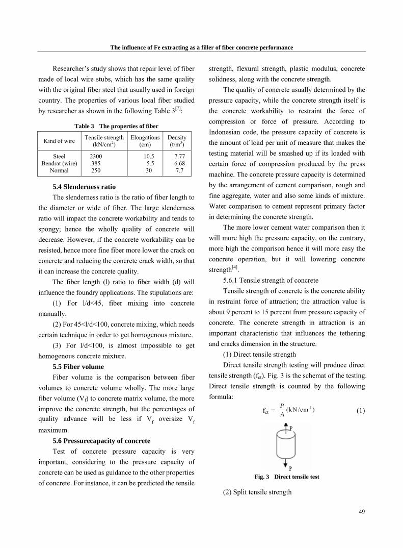
The influence of Fe extracting as a filler of fiber concrete performance
49
Researcher’s study shows that repair level of fiber made of local wire stubs, which has the same quality with the original fiber steel that usually used in foreign country. The properties of various local fiber studied by researcher as shown in the following Table 3[7]:
Table 3 The properties of fiber
Kind of wire Tensile strength(kN/cm2)
Elongations (cm)
Density(t/m3)
Steel Bendrat (wire)
Normal
2300 385 250
10.5 5.5 30
7.776.687.7
5.4 Slenderness ratio The slenderness ratio is the ratio of fiber length to
the diameter or wide of fiber. The large slenderness ratio will impact the concrete workability and tends to spongy; hence the wholly quality of concrete will decrease. However, if the concrete workability can be resisted, hence more fine fiber more lower the crack on concrete and reducing the concrete crack width, so that it can increase the concrete quality.
The fiber length (l) ratio to fiber width (d) will influence the foundry applications. The stipulations are:
(1) For l/d<45, fiber mixing into concrete manually.
(2) For 45<l/d<100, concrete mixing, which needs certain technique in order to get homogenous mixture.
(3) For l/d<100, is almost impossible to get homogenous concrete mixture.
5.5 Fiber volume Fiber volume is the comparison between fiber
volumes to concrete volume wholly. The more large fiber volume (Vf) to concrete matrix volume, the more improve the concrete strength, but the percentages of quality advance will be less if Vf oversize Vf maximum.
5.6 Pressurecapacity of concrete Test of concrete pressure capacity is very
important, considering to the pressure capacity of concrete can be used as guidance to the other properties of concrete. For instance, it can be predicted the tensile
strength, flexural strength, plastic modulus, concrete solidness, along with the concrete strength.
The quality of concrete usually determined by the pressure capacity, while the concrete strength itself is the concrete workability to restraint the force of compression or force of pressure. According to Indonesian code, the pressure capacity of concrete is the amount of load per unit of measure that makes the testing material will be smashed up if its loaded with certain force of compression produced by the press machine. The concrete pressure capacity is determined by the arrangement of cement comparison, rough and fine aggregate, water and also some kinds of mixture. Water comparison to cement represent primary factor in determining the concrete strength.
The more lower cement water comparison then it will more high the pressure capacity, on the contrary, more high the comparison hence it will more easy the concrete operation, but it will lowering concrete strength[4].
5.6.1 Tensile strength of concrete Tensile strength of concrete is the concrete ability
in restraint force of attraction; the attraction value is about 9 percent to 15 percent from pressure capacity of concrete. The concrete strength in attraction is an important characteristic that influences the tethering and cracks dimension in the structure.
(1) Direct tensile strength Direct tensile strength testing will produce direct
tensile strength (fct). Fig. 3 is the schemat of the testing. Direct tensile strength is counted by the following formula:
fct = 2(kN /cm )PA (1)
Fig. 3 Direct tensile test
(2) Split tensile strength

The influence of Fe extracting as a filler of fiber concrete performance
50
According to Wang and Salmon (1993, p. 11), split tensile strength testing done by using laid cylindrical tester down and added by steel plate with the up and down part dimension is 30×12 mm. Fig. 4 is the schemat of the testing. By giving pressure to the diameter hence the cylinder will be split (Murdock, 1986, p. 9).The split tensile strength testing can be counted by using the formula below:
fct=22 ( k N /c m )P
ld=
π (2)
Fig. 4 Split tensile strength testing
(3) Bending tensile strength In this testing, tensile strength is used bending
tensile strength testing because this test is almost close by the real tensile strength in its application in the field. However, it doesn’t mean that bending tensile strength is the better testing method than the other method. In this bending tensile strength testing, the tester used is beam with dimension 15 cm × 15 cm × 60 cm and its maximum aggregate is 40 mm. The load application method is through one load in the centre point until the tester is cracking. Fig. 5 is the schemat of the testing. Tensile strength in bending refers to the modulus of rupture. It is counted according to the American Standard for Testing Material (ASTM), which also important in determines the crack and beam deflection. This tensile strength produces higher tensile value then cylindrical trial, because of non-linear distribution at the concrete tension in tensile destruction.
5.6.2 Aalysis result Here we change the fiber’s composition and the
WCR, and give the curves about split tensile strength,
compression strength and flexural strength (Fig. 6-Fig. 11). Table 4 is the results of these testings.
5 cm 5 cm50 cm
60 cm
L/3 L/3L/3
P satumuatan
Fig. 5 Bending tensile strength testing
Fig. 6 The relation of fiber composition and split tensile strength
Fig. 7 The relation of fiber composition and compression strength
P
Komposisi campuran (%)
tegangan beton karakteristik (kg/cm2)
17.39114.767
18.172 19.618
tegangan betonkarakteristik
0 0.2 0.4 0.6 0.8 1.0 1.2 1.4 1.6
25 20 15 10 5 0
Komposisi campuran
123.767103.549 103.563
167.796
0
20
40
60
80
100
120
140
160
180
tegangan beton
karakteristik
0 0.2 0.4 0.6 0.8 1.0 1.2 1.4 1.6
tegangan Beton Karakteristik (Kg/cm2)
Komposisi campuran (%)
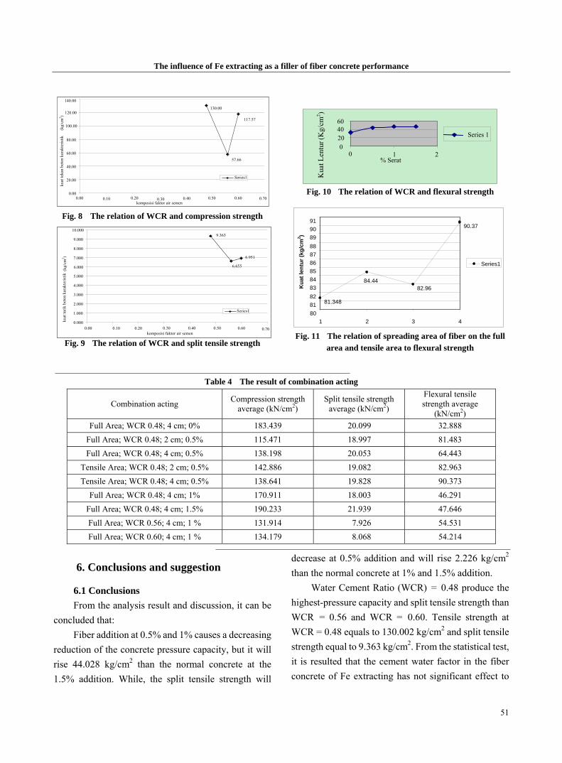
The influence of Fe extracting as a filler of fiber concrete performance
51
9.363
6.655
6.951
0.000
1.000
2.000
3.000
4.000
5.000
6.000
7.000
8.000
9.000
10.000
0.00 0.10 0.20 0.30 0.40 0.50 0.60 0.70
kuat
tarik
bet
on k
arak
teris
tik(k
g/cm
2 )
Series1
komposisi faktor air semen
Fig. 8 The relation of WCR and compression strength
Fig. 9 The relation of WCR and split tensile strength
Fig. 10 The relation of WCR and flexural strength
Fig. 11 The relation of spreading area of fiber on the full area and tensile area to flexural strength
Table 4 The result of combination acting
Combination acting Compression strength average (kN/cm2)
Split tensile strength average (kN/cm2)
Flexural tensile strength average
(kN/cm2) Full Area; WCR 0.48; 4 cm; 0% 183.439 20.099 32.888
Full Area; WCR 0.48; 2 cm; 0.5% 115.471 18.997 81.483 Full Area; WCR 0.48; 4 cm; 0.5% 138.198 20.053 64.443
Tensile Area; WCR 0.48; 2 cm; 0.5% 142.886 19.082 82.963 Tensile Area; WCR 0.48; 4 cm; 0.5% 138.641 19.828 90.373
Full Area; WCR 0.48; 4 cm; 1% 170.911 18.003 46.291 Full Area; WCR 0.48; 4 cm; 1.5% 190.233 21.939 47.646 Full Area; WCR 0.56; 4 cm; 1 % 131.914 7.926 54.531 Full Area; WCR 0.60; 4 cm; 1 % 134.179 8.068 54.214
6. Conclusions and suggestion
6.1 Conclusions From the analysis result and discussion, it can be
concluded that: Fiber addition at 0.5% and 1% causes a decreasing
reduction of the concrete pressure capacity, but it will rise 44.028 kg/cm2 than the normal concrete at the 1.5% addition. While, the split tensile strength will
decrease at 0.5% addition and will rise 2.226 kg/cm2 than the normal concrete at 1% and 1.5% addition.
Water Cement Ratio (WCR) = 0.48 produce the highest-pressure capacity and split tensile strength than WCR = 0.56 and WCR = 0.60. Tensile strength at WCR = 0.48 equals to 130.002 kg/cm2 and split tensile strength equal to 9.363 kg/cm2. From the statistical test, it is resulted that the cement water factor in the fiber concrete of Fe extracting has not significant effect to
130.00
57.66
117.57
0.00
20.00
40.00
60.00
80.00
100.00
120.00
140.00
0.00 0.10 0.20 0.30 0.40 0.50 0.60 0.70komposisi faktor air semen
kuat
teka
n be
ton
kara
kter
istik
(k
g/cm
2 )
Series1
81.348
84.4482.96
90.37
8182838485868788899091
1 2 3 4
Kua
t len
tur (
kg/c
m2 )
Series1
80
0204060
0 1 2% Serat
Series 1
Kua
t Len
tur (
Kg/
cm2 )

The influence of Fe extracting as a filler of fiber concrete performance
52
the pressure capacity and has significant effect to the split tensile strength.
The maximum rising of this bending tensile strength happens in 1.5% fiber addition that is 14.81 kg/cm2 from normal concrete. The result of statistical test shows that Fe extracting addition to bending tensile strength has significant effect.
The fiber spread in the tensile area is resulting higher bending tensile strength than the totally fiber addition or in whole part of concrete. Its average difference is equal to 3.705 kg/cm2.
4 cm fiber length results higher bending tensile strength than 2 cm fiber length. Its average difference is equal to 5.185 kg/cm2. The result of statistical test shows that variation of fiber length to bending tensile strength has not significant effect.
The combination result of some treatment that tested by using continued statistic test that is integrity different test resulted that to get maximum pressure capacity and bending tensile strength of concrete uses concrete combination with the percentages of fiber addition 1.5% FAS 0.48 total spread area, and 4 cm fiber length. While for the maximum result of bending tensile strength of concrete given by the concrete combination with the fiber addition percentages is 0.5%, 0.48 FAS, tensile spread area, and 4 cm fiber length.
6.2 Suggestion From the analysis result, hence there are some
suggestions that can be delivered, they are: In the tester producing, it should avoid the fiber
spreading together and it would be better if the fiber were asunder little by little and spread evenly in the mixture. If it doesn’t give any attention, then it will have a risk to cause the separate agglomeration of fiber
that will absorb the cement paste, hence it causes appearing many holes in the concrete.
It needs to be done the next research to multiply the treatment combination; hence it can produce the optimum strength of fiber concrete.
References: [1] American Concrete Institute ACI Committee 544. Guide
for Specifying, Proportioning, Mixing, Placing and Finishing Steel Fiber Reinforced Concrete, Report: ACI 544, 3R-93, 1993.
[2] Suhendro, B.. Laporan Penelitian Pengaruh Pemakaian Fiber Secara Parsial Pada Balok Beton Bertulang. Fakultas Teknik Universitas Gajah Mada, Yogyakarta, 1991.
[3] Qomariah, B. S.. Hubungan tegangan-regangan beton mutu normal dengan serat serpihan besi. Majalah Bistek, 2001, 9(1): 14-25
[4] Rochidajah.. Perilaku Lentur dan Daktilitas Balok Beton Serat Bertulangan Lebih yang Dikekang pada Jalur Tekan. Tesis, Pasca Universitas Brawijaya Malang, 2002.
[5] Bayasi, M. Z. and Soroushian, P.. Effect of steel fiber reinforcement on fresh mix properties in concrete. ACI Material Journal, 1992, 89(4): 369-374.
[6] Soroushian, P & Bayasi, Z.. Concept of fiber reinforced concrete. Proceeding of the International Seminar on Fiber Reinforced Concrete. Michigan State University, Michigan, 1987.
[7] Park, R. and Paulay, T.. Reinforced Concrete Structures. New York: John Willey & Sons, 1975.
[8] American Concrete Institute ACI Committee 544. Measurement of Properties of Fiber Reinforced Concrete, Report: ACI 544, 2R-89, 1989.
[9] Dipohusodo, Istimawan.. Struktur Beton Bertulang. Gramedia Pustaka Utama, Jakarta. 1994.
[10] Nawy, E. G.. Beton Bertulang Suatu Pendekatan Dasar, PT. Refika Aditama, Bandung, 1998.
(Edited by Jenny)
May 2009, Volume 3, No.5 (Serial No.18) Journal of Civil Engineering and Architecture, ISSN 1934-7359, USA
53
The leasing operation of research of the office building market in China
QIU Guo-lin (Department of construction Management,School of Management of Jilin Architectural and Civil Engineering Institute,
Changchun 130021, China)
Abstract: The article analysis the external market environment and the situation of requirement and the competitor in market of office building with the same rank and the same type according to market research, the aim is to research the whole processing operation and management, including making the marker orientation, confirming and finding the potential lesse making the rent plan, negotiating and signing the contract. Key words: market research; lesse; rent; negotiation
1. Office market dynamics of model
1.1 Office market: the use of market, investment markets and market development[1]
As the market for office space with a high degree of market-oriented operation, the policy interventions small, the characteristics of high profit margin, investors favored the real estate investment tool, also known as real estate investment market “leader”.
Office market is for office space in the sum of all transactions, including supply and demand between the two sides, such as the sale or lease transactions and activities developed in the course of the transaction price, rent levels, the vacancy rate, yield, and so on. Office market by the use of market, investment markets and the development of a market: the market for office space refers to the use of office space by the supplier (the owners) and demand (the tenants) together form the office property market and the resulting set of market variables, such as rent, price, the vacancy rate; office investment market for office space it refers to as an investment tool and the formation of the entire investment market a part of the development of the market for office space refers to
QIU Guo-lin, professor; research fields: project management theory research and teaching. E-mail: [email protected].
the use of office space demand and investment demand for the formation of the property development market. The three market mutual contact and mutual, common decisions and affected the office market development.
The use of the office market supply and demand determine the market rent, price, and the vacancy rate. The use of the information office market will quickly back to the investment market, office rents and prices to determine the value of the investment office. This development costs and investment value of the relationship between the expectations of investors and investment income levels of new office space has driven the development of the project. In addition to the investment market for office space by the use of market impact, but also by the broader capital market. Investors will be office space and other investment vehicles weigh and compare, compare the results will eventually be reflected in investor demand by the rate of return on investment. Lags behind the supply impact of the use of market supply and demand for office space, rent and the market price, thereby affecting the investment market for office space investment income level.
In 1994, the American scholar Keogh established the relationship between model. The model can be used to image shows the use of the market, investment and development activities in the mutual dynamic role. Users of the information market will quickly back to the investment market, and then transferred to the investment market by the development of the market, decided to develop activities. At the same time, the market will be greater investment in the capital market.
The leasing operation of research of the office building market in China
54
Users of the market and the impact of changes in investment market development of the market, create demand for the development of the market, and the corresponding development of the market for the other two market supply.
1.2 Office rental market model[2] Tsolacos and McGough (1998) to the Keogh
based on the theory, combined with user market and the investment market and its impact on the mutual development activities, the establishment of the office market dynamics of the model.
Users of market demand and supply determine the market rent. The use of office space needs and national economic strength related activities, in particular by the office of the office of industry activities. National economic strength and trends can be used to represent GDP in the office of the office with activities in the banking industry, financial and insurance industries (BFI: banking, finance, and insurance sector) in the employment rate to represent. The supply of office space with new production from that office, but truly effective supply should also include the existing stock of vacant part. Therefore, with output as the supply of new office space on behalf of the suitability of the need to look at the vacancy in the stock relative to that part of the new part is obvious.
In office rentals in the equation of the change is the assumption that rents for office space from the projected demand and new supply decisions. Current demand is expected to previous years and changes in the GDP, the current and previous years in the BFI changes in the employment rate of the linear combination of new supply is the current and previous years in office completed a linear combination. So rent is GDP, BFI and the employment rate for office space completed in a linear sequence of their growth portfolio, which BFI GDP and employment rate is positive effect, the office of the completion of a negative effect, this is because the new office space to
meet the investment needs of some, thereby inhibiting the rent increase. Rent equation is as follows:
20
scv
t s t ss
V v R−=
Δ =α + Δ∑
20 0
QMSP OFBO GDP
m t m q t q tm q
p V V V− −= =
+ Δ − ω Δ +ε∑ ∑ (1)
I
i
GDPitit VR
01 βα +Δ+=Δ ∑
=−
t
K
k
GFBOktk
I
j
BFIjti VV 1
00
εωγ +Δ−Δ+ ∑∑=
−=
−
(2) In the equation, △ for the change of; R is the
actual rent levels; VGDP is the value; EBFI industry is in the employment rate; VOFBO the private sector is the number of completed office space; α, β, γ, ω are often factors; i, j, k are the years; ε1t is the occasional error[3].
2. Office market investment model
According to Keogh’s theory, there are three key office investment market forces influence the value of the assets.
First, the demand side, the existing office space and expected level of rent will affect the value of the assets, rents and demand is directly proportional.
Secondly, is still the demand side, the value of assets by the office of the investment objectives of the impact of yield. Yield goal is to invest in other comparable office space investment opportunities in the existing income level, the level of expected income and relative risk level of function. According to economic theory, investment opportunities in the pricing of any deviation will lead to investment flows, investment opportunities that various risks and benefits are balanced. In the model, stock price volatility to changes in economic conditions that investors in the office and investment preferences.
Finally, the market supply side, the development of the market to new supply, such attacks will increase in the yield fell to the asset value of negative effects.

The leasing operation of research of the office building market in China
55
The market value of the assets investment equation is as follows:
s
ssts
cvt RvV
02α Δ+=Δ ∑
=−
t
Q
q
OFBOqtq
M
m
SPmtm VVp 2
00εω +Δ−Δ+ ∑∑
=−
=−
(3)
2.1 Office market development model Office development model main factors affecting
office building obviously. The development and construction of the office
space rent and the value of the assets, because they represent the user and investment market conditions, these two factors and that the situation over the past few years to be included in the equation. In addition, the new development will be of short-term financing costs, so as a short-term interest rates also explain variables, have a negative effect. Short-term interest
rates can also be used as the future economic expectations, this is expected to affect the expected demand for office space. The completion of the development of the market equation is as follows:
nt
N
0nn3
OFBOt RsV α Δ+=Δ ∑ −
=
t3INTh-t
H
0hh
CVt
0rfVg εφ
φφ +Δ−Δ+ ∑∑
=−
Φ
=
(4)
This equation is meaning the actual short-term interest rates, s, g, f are constant coefficients; n, h are years; ε3t is the chance for error[4].
To sum up, the rental market for office space, the value of assets and the completion of a number of factors and indicators as shown in Table 1.
Table 1 The influencing factor of the office building market curcil Variable explained Influencing factor Explaining variable
Rent Economic active; BFI level; supply GDP varial; BFI level; rea Assets value Rent level; share price; Rent vraial; hare price varial
Area Rent level; asset value; active short interest rate
Rent varial; asset value varial; active short interestrate rate varial
The use of statistical data and regression analysis, various factors can be calculated, as well as make sure to explain the variable delay (in previous years of data to be interpreted variables are obvious role), quantitative come to rent, the value of assets and the number of completed The equation, and thus of GDP, BFI employment rate, rent, office space completed volume, stock prices, the interaction between the interest rate[5].
3. The investment management market for office space
The main mode of operation for office space is leasing business, that is the ultimate occupier (users) rather than primarily through the purchase of leased way to get the right to use the office space. Therefore, the rental management office to become the core of
investment management market. Office market in general the investment management market research from the start, first of all, the market environment, the same level with the type of market demand for office space and an analysis of competitors, and so on, and on the basis of this market positioning, then identify and find potential lessees To develop programmes rent, lease negotiations and a final contract.
3.1 Office tenant choice[6] Choice of the tenant, to consider the main criteria
for a potential tenant by the type of business and its reputation, financial stability and long-term profitability of the capacity of the required size and the need to provide the special property management services.
Property management companies must be careful analysis of each tenant to the credibility of the office
The leasing operation of research of the office building market in China
56
rental property affected. Potential lessees should be content with the business office of the lessee has been operated by the content of coordination, its credibility should be able to strengthen the overall image building. Property management companies should also analyse the potential lessees engaged in business in the process of financial stability, as it relates to potential lessees of the lease period stipulated in the contract whether the obligation to pay the rent on time. From the tax authorities, business administration, bankers, brokers and financial statements provided by the lessee to determine its credibility and financial position.
Tenant selection process of one of the most complex office building is to determine whether there is sufficient space to meet the characteristics of a particular tenant needs, to meet the leasing of space to the area of the specific needs, which often determines the potential The lessee can become a reality the lessee. In considering whether a suitable area for leasing space can be used often to consider the following three aspects: (1) Of the combination of buildings, whether a separate portfolio of rental units to meet a certain Rent-seeking characteristics of the needs. (2) Rent-seeking to experience the nature of business, some agencies need to be able to separate the office, and often can hope that these offices along the exterior of the building layout, to be able to receive adequate natural light and broaden their horizons. But there are also some companies may not want to have too much room and around the external walls. (3) To lease office space to future expansion plans, if a company in the future expectations of a large-scale expansion must be considered in a building whether or how to meet their future business development needs, particularly when the rent-seeking, Hope that when his office on layout. In general, for each office staff of 15-20 m2 unit within the construction area of more appropriate, although each staff closed the office space in general need only 5-6 m2. However, reception room, conference rooms, traffic area, storage space, office equipment and the
size of the public activities area than office space may be to increase the number of indicators.
Some rent-seeking, for the smooth conduct of its business, the need to provide some special services, property management companies have provided a greater difference in standard services, property management companies if not properly consider these issues in the future management of the property on the May be many contradictions. In accept or reject the special requirements of potential tenants, property management companies and owners should consider leasing the entire period of the actual expenses and costs - benefit ratio, in the future in order to determine who should bear the contract special services. For example, a company to install a computer workstation, as the workstation need to consume a large amount of electricity, may be more than office building in the supply line load some lessees need additional independent of the cooling system; some tenants to install themselves as the larger Equipment, the bearing capacity of the building has put forward higher requirements. To meet these requirements may be a lot of money and construction equipment of the system also may bring some trouble. However, property management companies or owners may have to consider a result of the favorable factors, such as the initial installation of such equipment could put the future installation of other equipment convenient, and rent-seeking are very clear and its subsidiary construction equipment or installation of the equipment of the work And the cost, it is likely to seek a long-term leases, in order to avoid repetition of such investment.
3.2 Determine the rent for office space Determine the rent for office space, the general
should seriously consider the following three aspects: (1) Or can be calculated using the lettable area Accurate measurement of the importance of this
relationship to ensure whether the property rental income and maximize the value of the property market.
The leasing operation of research of the office building market in China
57
Office space in the measurement when there are three very important concept, that is, building area, and the lettable area of rental units within the construction area. According to the relevant provisions of the Ministry of Construction, the construction area of the country “construction area of the rules” calculation; rental unit within the construction area, including the use of units within the area, external wall, the wall between the units and common units and the construction of the separation barrier between space The level of projected area of half a lettable area of rental units within the construction area with sharing the common construction area (including: elevator shaft, stairways, bathrooms, transforming rooms, equipment rooms, public foyer, aisle, the basement, on duty Jingwei Shi , And other functions for the entire construction services on the use and management of the public release of the construction area, rental units and public building space between the wall and the external walls of the wall half the level of projected area). In the calculation of sharing the common construction area, who have the use of space rental as an independent in the basement or garage as well as air defense projects not included in the basement of the building area of sharing common parts. Each of the independent rental units, following:
Each of the independent rental units yuan = lettable area of rental units within the construction area × (1 + construction area sharing common factor), the building area of sharing the common factor = entire building including the common area of building the entire rental unit and the construction area.
A commitment to lease the area who can be part of one floor, may also be the whole floor or several layers of the floor. For the whole of the lease, the tenant, the tenant must not only share in their common floors of the building area, but also sharing the bottom hall and all other services for the lessee or the use of the common construction area. General construction of the common area of old-sharing factor is much
greater than the new construction. The office building, sharing the common factor of 0.2 to 0.3 in between.
(2) Develop rental programme[7] The level of rents for office space depends
largely on local real estate market conditions. Determine the rent, according to the owners should generally be the first to achieve the investment objectives and its yield an acceptable minimum level of rent (that is, able to cover mortgage debt service, operating expenses and loss of vacant rental) to determine a basis for rent. When calculated based on the rent higher than market rents, property management companies to consider lowering operating costs so that the basis for a downward adjustment to the rental market rent levels.
In certain market conditions, an office property in the overall level of rental property itself depends mainly on the situation and the position. But office construction within a specific rental unit rent is based on the entire building in which the location of a certain difference, in terms of high-rise building more obvious. Property management companies in determining the rent for office space rental units, the common position of better rental units over the rental income to balance the bad location of the rental income rental units so that the entire building, the average rent for office space remained at slightly higher than the base rent Level.
(3) Rental units the size of the planning and interior decoration
When the tenant selection office is very concerned about their lease part of the effective use of their employees and can provide a comfortable working environment. Property management companies can be considered a lessee of the scale, organization structure, preferences and tastes, the need to install the equipment and financial capacity to pay,
(to be continued on Page 62)
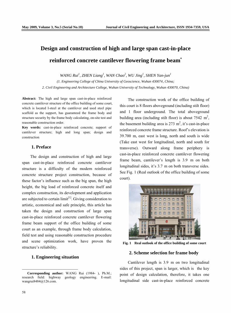
May 2009, Volume 3, No.5 (Serial No.18) Journal of Civil Engineering and Architecture, ISSN 1934-7359, USA
58
Design and construction of high and large span cast-in-place
reinforced concrete cantilever flowering frame beam*
WANG Rui1, ZHEN Liang1, WAN Chao2, WU Jing1, SHEN Yan-jun1
(1. Engineering College of China University of Geoscience, Wuhan 430074 , China;
2. Civil Engineering and Architecture College, Wuhan University of Technology, Wuhan 430070, China)
Abstract: The high and large span cast-in-place reinforced concrete cantilever structure of the office building of some court, which is located I-steel at the cantilever and used steel pipe scaffold as the support, has guaranteed the frame body and structure security by the frame body calculating, on-site test and reasonable construction order. Key words: cast-in-place reinforced concrete; support of cantilever structure; high and long span; design and construction
1. Preface
The design and construction of high and large span cast-in-place reinforced concrete cantilever structure is a difficulty of the modern reinforced concrete structure project construction, because of these factor’s influence such as the big span, the high height, the big load of reinforced concrete itself and complex construction, its development and application are subjected to certain limit[1]. Giving consideration to artistic, economical and safe principle, this article has taken the design and construction of large span cast-in-place reinforced concrete cantilever flowering frame beam support of the office building of some court as an example, through frame body calculation, field test and using reasonable construction procedure and scene optimization work, have proven the structure’s reliability.
1. Engineering situation
Corresponding author: WANG Rui (1984- ), Ph.M.;
research field: highway geology engineering. E-mail: [email protected].
The construction work of the office building of this court is 8 floors aboveground (including stilt floor) and 1 floor underground. The total aboveground building area (including stilt floor) is about 7542 m2, the basement building area is 273 m2, it’s cast-in-place reinforced concrete frame structure. Roof’s elevation is 39.700 m, east west is long, north and south is wide (Take east west for longitudinal, north and south for transverse). Outward along frame periphery is cast-in-place reinforced concrete cantilever flowering frame beam, cantilever’s length is 3.9 m on both longitudinal sides, it’s 3.7 m on both transverse sides. See Fig. 1 (Real outlook of the office building of some court).
Fig. 1 Real outlook of the office building of some court
2. Scheme selection for frame body
Cantilever length is 3.9 m on two longitudinal sides of this project, span is larger, which is the key point of design calculation, therefore, it takes one longitudinal side cast-in-place reinforced concrete

Design and construction of high and large span cast-in-place reinforced concrete cantilever flowering frame beam
59
cantilever structure as an example to calculation and design.
2.1 Scheme assumption According to the location at the upper air, large
span and big load of cantilever concrete structural plane it, based on the actual situation of construction site and previous construction experience,we had preliminarily considered several following projects:
Scheme one is using steel pipe to put up three rows of landing scaffolds.
Scheme two is consulting with construction unit and design unit to replace cantilever concrete structural plane with steel structure.
Scheme three is putting up cantilever frame to compose steel platform as construction bearing operation area.
2.2 Scheme’s technical analysis and comparison
For the scheme one, landing scaffolds occupy many steel pipes, the cost is expensive (high), the construction period is long and more labor is wasted.
For the scheme two, construction technology is complex, it needs design unit to carry on structural design anew but the building owner doesn’t agree on.
For the scheme three based on scheme one we carry on the optimization, it relatively reduces the cost and shortens the construction period, moreover it is verified by experts that it can reach the request of technical quality and safety.
Synthetically considering feasibility, security, efficiency of each project, we select scheme three which puts up cantilever frame for this project.
3. Design for frame body
In Fig. 2 (Down-looking planar graph of cantilever flowering frame beam), the position which blackbody shows is cantilever flowering frame beam.
Cantilever which is on one longitudinal sides of this project mostly is used method of hanging each layer, namely from the seventh floor to the eighth floor
and then to the roofing layer, finally to flowering beam, withstand superstructure’s cantilever steel pipe or bottom die of cantilever beam by diagonal brace from under layer in turn. The transverse distance of diagonal brace steel pipe is 1 m, setup longitudinal link rod which drawing pace is 1.2 m.
Fig. 2 Down-looking planar graph of cantilever flowering frame beam
External frame which is on two longitudinal sides of this project that put up from the third floor, therefore it used external frame to support bottom die of cantilever beam, simultaneously, it needed to take some reinforcement measures to brace stiffness and strength of diagonal brace steel pipe. First, put up two rows of support frames closely at the edge of the eighth layer and its distance is 1.50 m, and the spacing is 0.8 m. The sweeping pole is 0.2 m away from floor and its drawing pace and span are all 1m; two rows of support frames touch to the floor’s top surface, meanwhile steel pipe thick column hoop and two rows of floor’s support frames are connected together with steel pipe and then on the seventh floor, the eighth floor and the roofing layer connect and fix steel pipe thick column and cross bar which is on diagonal brace steel pipe of the seventh floor, its vertical distance is 1.2 m; meanwhile connect diagonal brace frame and two rows of vertical support frame which is on the floor as well as external frame in together transversely, its drawing pace and span is 1.2 m and 1 m; then connect diagonal brace steel pipe and thick column hoop with steel pipe which are knotted vertically to diagonal brace steel pipe by setting two

Design and construction of high and large span cast-in-place reinforced concrete cantilever flowering frame beam
60
tensile nodes which is set in the 1/3 of diagonal brace steel pipe. Ensure that diagonal brace frame and external frame as well as inner brace frame are connected firmly. See Fig. 3 (Elevation drawing of cantilever frame’s support system).
Fig. 3 Elevation drawing of cantilever frame’s
support system
Fig. 4 Real photo of putting up construction of
cantilever frame
In the roofing level, it’s the bottom of flowering frame at the 38.750 m elevation, there is no application point on the apex of two rows of setting inner vertical support frames, therefore, in this layer connect two rows of vertical support frames and inner frame of roofing level with transverse steel pipe to keep them together, simultaneously, because the pillar which is at the roofing is free end, the pillar which is nearby edge of the floor is connected to the pillar which is in the floor with steel pipe column hoop in together. Moreover, because this project uses external frame to bear partial load, therefore, we carry on whole reinforcement to external frame. The concrete reinforcement method is that connecting two rows of external frames which is on both longitudinal sides from the third the floor to the sixth floor and side column which is in relevant floor with thick column hoop in together. In order to reflect situation for scaffolding condition of support, photographs scene photo of field scaffolding as follow Fig. 4.
4. Checking calculation for structural stability
Put up steel pipe which height is 11.15 m and the deviation vertical direction angle is 20 degrees, carry on the checking calculation to steel pipe’s bending strength[2]:
4.1 Load calculation (1) Permanent load Standard of template’s dead weight: 1 kN×0.85×0.85 = 0.73 kN Dead weight of fresh concrete floor: 2.4×9.8×0.9×0.4×0.85 kN =7.19 kN Dead weight of steel bar: (4×3.85×0.85+4×2.98×0.85+8×1.21×0.85+5×5.3×0.395) ×9.8 N =410.71 N NGK=0.73+7.19+0.41 kN =8.33 kN (2) Construction load Standard of construction and equipment load: NQK=0.3 kN×0.85×0.85 =0.22 kN
Design and construction of high and large span cast-in-place reinforced concrete cantilever flowering frame beam
61
4.2 Checking calculation for bending strength Strength of vertical direction is: N = 1.2×8.33 kN+1.4×0.22 kN = 10.30 kN Strength of direction which is vertical to pole is: N1 = N×sinθ = 10.30 kN×sin20° = 3.52 kN Bending moment value: M = N1·L = 3.52×0.21 kN·m = 0.739 kN·m
= 739 N·m Modulus of steel pipe section: W = 5.08 cm3 Checking calculation for strength: σ = M/W = 739/5.08 N/mm2=145 N/mm2
< f = 205 N/mm2 Therefore steel pipe’s bending strength meet the
requirement.
5. Design for pressure test
5.1 Choose of pressure test’s scheme In order to ensure the safety of construction for
high and large span cantilever support frame, determine stress condition of each frame body’s member and deformation condition of frame body, put up test frame on the biggest stress position before construction. Use method of uniform load for pressure test, according to actual dead weight of reinforced concrete, dead weight of template, live load of construction and equipment, put them together, multiply by 1.2 time of safety factor, then according to 1.2 time of gross weight, accumulate relevant weight on laying plate. Take observation for the biggest settlement of frame body through theodolite, and acquisition and analysis for the biggest stress value of member auxiliarily using stress instrument.
5.2 Calculation of the biggest load The position of the biggest stress position is in the
○D /○5 —○6 axes. Concrete volume V = 9.132 m3, weight of
concrete M = 9.132 m3×2.4 t/m3 = 21.92 t, weight of steel bar is 1.7 t, therefore gross weight of reinforced concrete is G1 = 23.62 t.
Weight of per square template is 0.01 t, area is 92.26 m2, therefore, the weight of template is G2 = 0.01 t/m2×92.26 m2 = 0.92 t.
Construction live load and equipment load are 300 kg per square, total plane area is 30.24 m2, construction live load is G3 = 0.3 t/m2×30.24 m2 = 9.072 t.
Gross weight is F = 23.62 t+0.92 t+9.072 t = 33.61 t, load of unit area is 33.61 t/30.24 m2 = 1.11 t/m2.
5.3 Design for pressure test’s scheme Use sandbag to accumulate load respectively on
test frame, 1st accumulate load to 70% of gross weight, named N1 = 33.61×0.5×0.7 t = 11.76 t; 2nd accumulate load to 90% of gross weight, named N2 = 33.61×0.5×0.9 t = 15.12 t; 3rd accumulate load to 100% of gross weight, named N3 = 33.61×0.5×1 t = 16.8 t. If test frame’s various data is at the limit range of calculated value, then the project of using support frame is safe and reliable, so it can be use to the formal project construction.
6. Key constructions
(1) Good steel pipe for support steel pipe is necessary and serious rusting, deformed, crooked steel pipe are forbidden to use. Steel pipe of diagonal brace must be a whole and two butted steel pipe are forbidden to be used for diagonal brace.
(2) Fastener which is used to put up external frame must be guaranteed completly, should not allow mutilated fastener to be used to diagonal brace frame. Only must pass through acceptance when putting up is finished then it may pour concrete. In process of pouring concrete, it needs to send special man to nurse support system and should be solve promptly if finding case as subsidence, loosening, deformation[3].
(3) Strictly controll actual construction load must be strictly controlled in order not to exceed design load, relevant control measures must be drafted and if it exceeds maximum load, materials like steel bar and so on it can not be stacked above support.
Design and construction of high and large span cast-in-place reinforced concrete cantilever flowering frame beam
62
(4) Pumping concrete can’t be poured directly into beam slab which is at the point of cantilever, but should be poured on construction platform which at the inside of cylinder, be shoveled to position of cantilever by man to reduce pumping concrete to impact cantilever position. Vibrate concrete from far to near as possible and make sure that there is nobody standing on the top of cantilever[4].
7. Conclusion
(1) Using common fastener and steel pipe, by the method of cantilevering layer by layer to put up high and large span cantilever support frame, it does not need increase other tools and materials, operation is simple and quick, construction cost is inexpensive.
(2) In the process of making project (scheme), we should carry on comprehensive and painstaking plan, ensure that design calculation is detail and exact, construction method is proper, measure is reasonable.
Check strictly in implementation process, put up according to design project and do conscious informatization construction work to ensure the quality and safety.
(3) This high and large span cast-in-place reinforced concrete flowering beam support system has characteristics such that construction is simple, construction period is short, it’s economically viable, may provide experience reference for similar project.
References: [1] DING Wei, PU Jian-yun. Cantilever Fastener-Style Steel
Pipe Scaffold Apply in Extra-High Building Construction. [2] GB5001722003. Design Standard of Steel Structure. [3] JGJ13022001. Safety Technology Standard of
Construction Fastener-style Steel Pipe Scaffold. [4] Compilation Group of Construction Handbook.
Construction Handbook. Beijing Building Industry Press, 2003.
(Edited by Jenny)
(continued from Page 57)
and so on to help identify the best single tenant size, and its lease on the rental unit within the room layout, office equipment layout, the internal arrangements for access to design. References: [1] WANG Cheng-qing, NI Peng-fei. Chinese estate periodic
fluctuation: Explanation of transfer and chance policy. Finance and Economy, 2002, (9): 80-91.
[2] TAN Gang. Research of the estate periodic fluctuation in Shenzhen. Construction Economy, 2001, (7): 59-68.
[3] YE Yan-bing and DING Lie-en. Design and research of estate alarm index system. Optimization of Capital Construction, 2001, (5): 39-41.
[4] ZHAO Li-ming and JIA Yong-fei. Research of Estate Alarm System, Press of Tianjin University, 199: 52-54. LI Ang. Eemulational Research of System Dynamics of Estate boom Cycle, Construction Management Institute in Qinghua University, 2002, (6): 25-30.
[5] LI Zi-nai and YE An-zhong. High Measure Economics. Changchun: Qinghua University Publishing Company, 2000, 56(11): 12-16.
[6] ZHANG Tao, GONG Liu-tang and PU Yong-xiang. On the asset return, mortgage lending and property price. Journal of Finance, 2006: 24-25.
[7] WANG Cheng-qing, NI Peng-fei. Chinese estate periodic fluctuation: Explanation of transfer and chance policy. Finance and Economy, 2002, (8): 25-31.
(Edited by Jenny)