joint seismic tomography for bulk sound and shear wave...

JOURNAL OF GEOPHYSICAL RESEARCH, VOL. 103, NO. B6, PAGES 12,469-12,493, JUNE 10, 1998

Joint seismic tomography for bulk sound and shear wave speed in the Earth's mantle

B.L.N. Kennett and S. Widiyantoro 1 Research School of Earth Sciences, Australian National University, Canberra

R.D. van der Hilst

Department of Earth, Atmospheric and Planetary Sciences, Massachusetts Institute of Technology, Cambridge

Abstract. High-quality P and S travel times are now available from careful reprocessing of data reported to international agencies. A restricted data set has been extracted,for which comparable ray coverage is achieved for P and S, and used for a joint inversion to produce a three-dimensional model for shear and bulk sound velocities represented in terms of 2 ø x 2 ø cells and 18 layers in depth through the mantle. About 106 times for each of P and S are combined to produce 312,549 summary rays for each wave type. Linearizing about the ak135 reference model, 583,200 coupled tomographic equations are solved using an iterative partitioned scheme. Clear high-resolution images are obtained for both bulk-sound speed and shear wavespeed. The bulk and shear moduli have differing sensitivity to temperature and mineral composition, and so the images of the two velocity distributions help to constrain the nature of the processes which produce the variations. Different heterogeneity regimes can be recognised in the upper mantle, the transition zone, most of the lower mantle, and the lowermost mantle. In the upper mantle, many features can be explained by thermal effects; but in some orogenic zones (e.g. western North America), the opposite sense of the bulk-sound and shear wave speed variation requires compositional effects or volatiles to outweigh any thermal effects. In the lower mantle, pronounced narrow structures which may represent remnant subduction are most marked in shear. The level of large-scale variations in bulk sound speed compared to shear diminishes with depth in the lower mantle reaching a minimum near 2000 km. Below this depth, the variability of both wave speeds increases. Near the core-mantle boundary the variations of the two wave speeds show little concordance, suggesting the presence of widespread chemical heterogeneity.

1. Introduction

The global seismological datasets of seismic events and arrival times, assembled by the International Seismological Centre and the National Earthquake Information Centre, con- tain a rich set of information on P and S travel times. The set

of more than 6 x 106 P times has been exploited by a number of authors, and it has proved possible to produce relatively detailed images of three-dimensional structure for large parts of the mantle [e.g., Inoue et al., 1990; Pulliam et al., 1993; van der Hilst et al., 1997] and more detailed structure in the upper mantle, either by specific regional studies superim- posed on a low resolution regional model [e.g., Fukao et al.,

•Now at Department of Geophysics and Meteorology, Bandung Institute of Technology, Indonesia.

Copyright 1998 by the American Geophysical Union.

Paper number 98JB00150. 0148-0227/98/98JB-00150509.00

1992; Widiyantoro and van der Hilst, 1996], a multicell inversion for the mantle to 1200 km depth [Zhou, 1996], or the use of variable cell size [Bijwaard et al., 1996].

In contrast, the available set of more than 106 S times has been used much less in tomographic studies, in part because of the greater scatter in the observations. Instead studies for three-dimensional S wave structure have been based on the

use of times derived from long-period body waves [e.g., Grand, 1994; Suet a/.,1994) or the matching of waveforms [e.g., Suet al., 1994). However, Vasco et al. [1994] have employed a relatively coarse parametrisation for the mantle for both P and S wave speeds and present P wave images down to the core-mantle boundary, but truncate the S results at 2270 km to avoid the influence of the cross-over with SKS

in the S travel times. Recently, Robertson and Woodhouse [1995,1996] have used the database from the International Seismological Centre (ISC) to perform inversions for both P and S models specified by spherical harmonics (usually restricted to orders less than 8) and have demonstrated a close proportionality between P and S wave heterogeneity in the lower mantle. Their S model initially extended to 2100 km

12,469

12,470 KENNETT ET AL.: JOINT BULK SOUND AND SHEAR TOMOGRAPHY

and was subsequently extended deeper into the lower mantle extracted the radial variation in the ratio of the heterogeneity following further processing of the S wave times. in P and S wave speeds v (= 0 In/•/0 In a) as a proxy for the

The utility of the S phase information has been significantly influence of the bulk modulus. In this study, we have been improved by careful reprocessing of the arrival time data sets [Engdahl et al., 1998]. When combined with careful processing of the travel times to separate S and SKS arrivals in the neighbourhood of the crossover near 83 ø, it is possible to determine three-dimensional S wave structure throughout the mantle at a comparable resolution to P. For example, van der Hilst et al. [1997] have used a 2øx2 ø cellular representation with 18 layers in depth for P and S waves. S wave times have to be picked in the coda of P and so the structural component in the arrival times has to be sought in the presence of other influences. Nevertheless, three-dimensional re-

sults for S wave speed of good quality are attainable from the inversions of the reprocessed bulletin data with, for example, clear images of subduction zones [Widiyantoro, 1997]. Good agreement is obtained with the high resolution S models derived from SH arrival times from long-period S records [Grand et al., 1997].

The datasets of P and S arrival times provide the most directly comparable information on different aspects of the Earth's internal structure. Now that high-quality images of three-dimensional structure are available for both P and S we

can start to address a number of significant issues, such as how far can the pattern of P wave heterogeneity be explained by just the variation in shear modulus? The proportionality in P and S heterogeneity for large-scale variations observed by Robertson and Woodhouse [1995,1996] would suggest that the contribution from the bulk modulus to P wave speed variation in the lower mantle is not large. Nevertheless, it is de- sirable to try to separate the contributions from the shear and bulk moduli, since the bulk modulus is of particular interest in laboratory experiments at high temperature and pressure. This separation been attempted by Su and Dziewonski [ 1997] using a representation in terms of low-order spherical harmonics.

Individual inversions for P and S structure are designed to make the best possible use of the available data sets and so do not usually have directly comparable ray coverage in the mantle. In addition, when the inversions for P and S wave

speeds are performed by different research groups, there are likely to be effects from different inversion strategies and techniques for regularisation. A partial solution is to undertake separate P and S inversions for mantle structure using a selected data set designed to achieve a common ray coverage. However, we prefer to take a more direct route and invert P and S travel times together for the three dimensional variations in bulk sound and shear wave speed using the "common ray" data set. Although we sacrifice some potentially interesting information by using a restricted data set we gain in the reliability of the bulk sound and shear wave speed images. We place a check on our joint inversion procedure by comparison with bulk-sound speed and shear wave speed results derived from independent inversions of the P and S times from the "common ray" data set.

Robertson and Woodhouse [ 1996] have examined the proportionality between P and S wave speed variations and have

able to determine the three-dimensional variation of bulk

sound and shear wave speed in the mantle, and can demon- strate that the variation of v with radius does not adequately characterise the fairly complex pattern of behaviour revealed in the joint inversion.

Recently, Su and Dziewonski [ 1997] have undertaken a simultaneous inversion of P wave travel times derived from the

iSC bulletins, long period waveforms including both body wave (P, PP, S, SS, etc.) and surface wave components, and travel times derived from long-period waveforms to produce three-dimensional models for the bulk sound and shear ve-

locity variations in the whole mantle. Their study uses a spherical harmonic representation to degree 12 and a Cheby- shev polynomial representation in radius (to order 13) and so does not achieve the resolution of such features as subduction

zones that we are able to achieve for a more restricted portion of the globe in our joint tomographic inversion. Further, Su and Dziewonski [ 1997] make use of data from a wide range of periods so that the corrections for anelasticity between different data sets take on a major significance.

In this study we use a higher resolution representation of the Earth's structure through a 2 ø x 2 ø cellular representation with 18 layers in depth as used by van der Hilst et al. [ 1997] for P and S waves. With this parameterisation for both the bulk sound and shear wave speed distributions, we are able to delineate features which are suppressed in a low-order spherical harmonic expansion such as the subducting slabs in the upper mantle. The joint inversion for bulk sound and shear wave speed provides us with a new tool to probe the proper- ties of the Earth's interior, since we are able to separate influences that were previously concealed in disparate P and S inversions. In particular we can begin to ask such questions as: (1) How much of the variation in P wave speeds can be explained by shear heterogeneity? (2) To what extent is the origin of the imaged heterogeneity likely to be due to thermal effects?

The merit of working with images of both the bulk sound and shear wave speeds arises from the differing sensitivity of the shear and bulk moduli to temperature and mineralogy. For instance, we would expect the effect of increased temperature to be such that both bulk-sound speed and shear wave speed would decrease, with slightly greater change in shear wave speed. At elevated temperature, changes in shear modulus may be rather larger than for bulk modulus; recent laboratory experiments show strong change in shear modulus as the solidus is approached [Tan et al., 1997].

When the bulk sound speed and the shear wave speed show comparable behaviour, it is reasonable to assume a thermal origin for the features in question. However, it is unlikely that thermal effects can be the sole cause when variations in

bulk sound speed are significantly larger than those in the shear wave speed. Further, when the variation in the bulk sound speed does not correlate with that for shear wave speed, we need to find an alternative explanation such as the presence of chemical heterogeneity or the presence of volatiles.

KENNETr ET AL.: JOINT BULK SOUND AND SHEAR TOMOGRAPHY 12,471

In the absence of mineral physics data for the full range 1.8. We need to recognise that the picking errors for S are of physical conditions encountered in the mantle, it is diffi- larger, and so the structural component of the deviations of S cult to provide a detailed interpretation of the wave speed im- times from a reference is more difficult to extract. ages. Nevertheless, we can recognise different heterogene- In order to use P and S information to determine the bulk ity regimes in the upper mantle and transition zone, in the sound and shear wave speeds at the same time, we need to be bulk of the lower mantle, and in the lowermost mantle. As careful that the superior quantity and quality of the P data do the core-mantle boundary is approached, there is very little not overwhelm the S results. We have therefore restricted at- concordance in the variations of the two wave speeds, which suggests the presence of widespread chemical heterogeneity.

The results we obtain are in general accord with those obtained by Su and Dziewonski [ 1997] but we see more correlation between the bulk sound and shear variations in the shal-

lower part of the mantle. The S structures agree well with those presented by Grand et al. [1997] in the areas of common data coverage and the P wave speed perturbations re- constructed from the bulk sound and shear wave distributions

are a somewhat muted version of those presented by van der Hilst et al. [ 1997] from a direct inversion of P travel time data.

2. Bulk-Sound and Shear Wave Tomography

tention to the P and S times for comparable paths, i.e., those for which P and S have a common source and receiver; the

data coverage of the mantle is reduced, but we have the com- pensation of equivalent coverage for the two wave types. The coverage in some parts of the upper mantle is restricted because we need both P and S phases to be reported; e.g., many seismic stations in North America, away from the active seismic zones, report dominantly P with few available S read- ings.

Approximately 106 P and 106 S data from the Engdahl et al. [1998] database have been used in all. We have included 9453 SKS data which helps to improve geographical coverage for S in the lowermost mantle. However, the requirement that the ray path coverage be comparable restricts the number of suitable SKS observations.

2.1. Data Selection

The arrival times for both P and S phases used in this study, and the event hypocentres, are taken from the global data set for over 80,000 events assembled by Engdahl et al. [1998]. The entire data catalogue of the International Seismological Data Centre, supplemented with more recent observations, has been relocated using a nonlinear scheme with the inclusion of the depth phases (pP, pwP) as well as the S and PKP phases, using the ak135 model of Kennett et al. [1995] as a radially stratified global reference. At each stage, the reported arrival times are reassociated with seismic phases using the improved locations to provide a set of travel times whose variance is significantly reduced compared with the original data catalogues. Over 35,000 events have been used in this study, recorded at one or more of over 3000 seismological stations around the globe.

We have used P and S wave arrival time data for distances

out to 105 ø and a limited amount of SKS data from 84 ø to

105 ø. Where crossovers in phase times occur, as at 83 ø for S and SKS, particular care has been taken by Engdahl et al. [ 1998] to ensure that the phase association was as effective as possible.

P wave arrival times are picked as first arrivals and only need to be distinguished from the ambient noise, and the typical standard deviation in the distribution of observed times

is of the order of 1 s. However, an S arrival has to be found

against the background of P coda, and the difficulty of picking is compounded by effect of attenuation in the Earth leading to lower-frequency arrivals. Nevertheless, following the event relocation and reprocessing, a consistent set of S arrivals has been produced with a standard deviation of 1.95 s, which provides an effective data set for tomographic inversion. The relative deviations in P and S travel times from the

reference values are therefore not so different, when we take

2.2. Joint Inversion for Bulk-Sound and Shear Structure

P wave travel times depend on the integral of the inverse of the P wave speed c• along the ray path from source to receiver. The P wave speed depends on the bulk modulus shear modulus/•, and density p through

o• 2 = (to -+- •/•)/D. (1) An S travel time is given by the ray integral of the inverse of the S wave speed/• which depends only on the shear modulus /• and density p,

•2 = t•/•. (2) From a knowledge of c• and/•, we can extract the bulk-sound speed ½

- • . (3)

Both P and S travel times thus depend on the shear wave speed/•, but only the P times involve the bulk-sound speed ½. The significance of ½ is that it depends on just the bulk modulus tc and density p, whereas the P wave speed depends on both tc and/•. Much of the experimentation at high pressures provides results that can be directly related to the bulk-sound speed ½.

To solve for aspherical variations in ½ and/•, we have developed a partitioned inversion scheme (see Appendices A and B) that balances the fit to the P and S wave data and uses both model and gradient damping. Fortunately, the iterative development is based on using cross-coupling terms (A20) which allows us to work alternately with each wave type so that the actual system of equations to be solved at a time is only half of all the equations. For the amount of data used (see below), the size of the system is within the compass of a powerful workstation. The solutions to the equation systems have been accomplished using a biconjugate gradient algo-

account of the typical P to S velocity ratio for the mantle of rithm LINBCG [Press et al., 1992].

12,472 KENNEq'T ET AL.: JOINT BULK SOUND AND SHEAR TOMOGRAPHY

:• S+SKS ß ! ß ! . ! ß

(a) (b)

i , i . i , , ! , ! , i ß

2 4 6 2 4 6

Number of iterations Number of iterations

Figure 1. Progress of the iterative joint inversion scheme: (a) linearized estimate of variance reduction for P times, and (b) linearized estimate of variance reduction for S times.

The joint inversion scheme described in the appendices has a double iterative component, the linear equation solver LINBCG is itself iterative, and the cross-coupling between bulk-sound speed and shear wave speed is included via a second iteration (A20). We have used seven iterations of the coupled inversion scheme, including both model norm and gradient damping, to ensure the stability of the resulting bulk- sound and shear wave speed images. The progress of the inversion can be followed in Figure 1. In the first iteration, no cross-coupling is introduced between the wave types (A21), and more than 25% of the data variance is explained at this stage. At the second iteration the cross corrections are introduced (A20); this leads to a change in the wave speed patterns, but after a further iteration the two slowness distributions are stabilized. After the fifth iteration, we have increased the number of iterations employed in the iterative equation solver (indicated by the solid symbols in Figure 1) and achieve a further slight reduction of variance. For the final iteration of (A20), the LINBCG algorithm was employed for 120 iterations in calculating each of inverses of the diagonal blocks of the Hessian matrix H•c •, H• which is sufficient to secure convergence in each case.

The linearized estimate of the variance reduction achieved

in the joint inversion is very similar for the two classes of data: 30% for P times and 28% for S times. Since we have

not included any event relocation parameters, all the variance reduction is accomplished with three-dimensional structure. This level of variance reduction is not as large as has been achieved in inversion of P times for P wave velocity alone (nearly 50% when relocation of events is allowed) but matches that achieved in direct inversion of S times for S

wave structure.

For this joint inversion, we have used the same parametrization for both bulk-sound speed and shear wave speed. Following the work of van der Hilst et al. [ 1997] for P waves, we have employed a representation in terms of 2 ø x2 ø cells in latitude and longitude with 18 layers in depth, giving a total of 291,600 cells. The representation in terms of 2øx2 ø cells will overparameterize the model in most parts of the mantle, and the 'structures which we discuss below span many cells.

The ray tracing in the various inversions has been carried out using the same reference model ak135 as in the relocation

procedure by Engdahl et al., [ 1998]. Information from event and station clusters based in 1 ø x 1 ø regions is combined into a single summary ray for each wave type (P or S ). The use of summary rays has the effect of reducing the uneven sampling of mantle structure by ray paths and also the computa- tion time required for ray tracing. The datum (residual time) assigned to the summary ray was the median of all data con- sidered for that summary ray; the number of rays that could contribute to the summary ray was not restricted. The total number of summary rays is 312,549 for P, and also 312,549 for S and SKS, leading to a linear system of 583,200 equations which has to be solved to extract the cellular representation of the three-dimensional bulk-sound speed and shear wave speed structure.

We did not invert for uncertainties in source location. The

selection of the ray paths for the joint inversion is designed to give the best possible common P and S coverage in the mantle, but the available azimuthal coverage of the available paths for each event is not necessarily suitable for further source relocation. We have therefore employed the hypocen- tral information from the reprocessed data set of Engdahl et al. [1998] which uses the same reference model ak135 as we have employed in the inversion, and all the data that we used here were also incorporated in the initial location procedure. The hypocenters after reprocessing are significantly improved from the original catalogues, particularly with re- gard to the depth of events.

Comparison of tomographic inversions with and without a relocation component indicates that with accurate initial locations, the inclusion of relocation may slightly affect the amplitude of the inferred variations but not the spatial patterns. In the joint inversion, we seek comparable fits to both P and S data rather than maximum variance reduction for

each set independently. The use of the hypocenters for the one-dimensional (l-D) reference model could produce mi- nor effects in the neighborhood of the source, for example, in the definition of subduction zones. However, the excel-

lent agreement of the S wave results from the joint inversion with an inversion for both structure and hypocenter mislo- cation using all available S wave data, as discussed below, provides additional evidence that the approximation of fixed hypocenters is not adversely affecting our results.

We did not employ specific station corrections as would be needed when using a low-order spherical harmonic basis for the structural components. With the relatively fine cellular parametrization that we employed, the shallow layers act to absorb the influence of corrections local to stations and

sources.

The ak 135 reference model is well suited for use as a base

model for travel time tomography because it was constructed to match empirical travel times constructed from averages of phase times from source and station pairs across the globe for a wide range of phases including P, S and SKS [Ken- nett et al., 1995]. This reference model should therefore have the effect of minimizing the potential residuals due to three- dimensional structure, so that a linearized inversion can be

undertaken. Following the work of van der Hilst et al. [ 1997] we have restricted the range of acceptable residuals for both

KENNETF ET AL.' JOINT BULK SOUND AND SHEAR TOMOGRAPHY 12,473

•_joint Layer: 6 520. -660. km

" "" • " •' • l

•_common

Perturbation [ %]

-1.00 0 1.00 -1.00 1.00 -1.00 1.00

Plate la. Comparison of the shear wave speed distribution from the joint inversion (/•_joint) with direct S wave inversions for the same set of S times (/•_common) and an inversion with the full set of available S phases [Widiyantoro, 1997]/•_full for layer centered at 590 km depth.


[•_.joint

: •-' ....., '•, ..•., ,• .... o -'•- '-:' • .•'• • ......................

, '•, ",.., ',,• , • •. 1.. ,.•,'

Layer: 11 1400. - 1600. km

[•_full

Perturbation [%]

! ' ! ............

-1.00 0 1.00 -1.00 1.00 -1.oo 1.oo

Plate lb. Same as Plate la, except for layer centered at 1500 km depth

KENNETF ET AL.: JOINT BULK SOUND AND SHEAR TOMOGRAPHY 12,475

Layer: O_joint 520. -660.

6

Perturbation [%]

-1.00 0 1.00 -1.25 1.25 -1.25 1.25

Plate 2a. Comparison of the bulk-sound speed distribution from the joint inversion (q•_joint) with estimates of bulk-sound speed extracted from independent P and S wave inversions using the same set of P and S times as in the joint inversion (q•_common) and separate P and S inversions using the full available data sets [van der Hilst et al., 1997; Widiyantoro, 1997] •p_full for layer centered at 590 km depth.


Layer: 11 •}._joint •400. - 1600. km

½•ommon •_ .• :..:••

Perturbation [% ]

-1.00 0 1.00 -1.25 1.25 -1.25 1.25

Plate 2b. Same as Plate 2a, except for layer centered at 1500 km depth.

KENNETI' ET AL.: JOINT BULK SOUND AND SHEAR TOMOGRAPHY 12,477

P and S residuals to q- 7.5 s so as not to stray too far from linear behavior. As a result we may well under-estimate the level of heterogeneity for some shallow structures since, for example, travel-time residuals can easily reach -10.0 s for Sn ray paths travelling through a fast craton.

However, in the interpretation of the inversions for two different wave speeds we need to be mindful of the potential influence of the reference model. Although the model ak135 gives a good representation of P and S travel times across the globe, in any particular area it may well not be optimum. We should therefore only place credence in significant differences in bulk-sound and shear wave speed variations.

2.3. Comparison With Alternative Inversions

In addition to the joint inversion procedure to generate both bulk-sound and shear wave speed models, we have undertaken independent tomographic inversions to generate images of the variation of bulk-sound speed and shear wave speed.

We consider two different classes of comparison. First, we have used exactly the same data set as has been employed in the joint inversion for both S (with a small amount of SKS data) and P. We have then performed inversions for three- dimensional structure for S and P waves separately using the LSQR algorithm of Nolet [1990] without an allowance for event relocation. The same style of gradient and model norm damping was employed as in the joint inversion. Second, we have used the results of inversions which exploit the full set of available data: for P wave structure we use the results of

van der Hilst et al. [ 1997] and for S wave structure we use the work of Widiyantoro [1997], which combines S travel times with SKS times from 83 ø to 105 ø to improve S resolution in the lower mantle. The two inversions of the full data sets

have been carried out using the same damping parameters to minimize artefacts arising from variable smoothing, and in- clude event relocation.

We compare the results obtained for S structure in the three different inversions for two different depths in the mantle (590, 1500 km) in Plate 1. The top panel in each display is the shear wave speed extracted from the joint inversion of P and S times, the middle panel is the S structure obtained by direct inversion of the S data set used in the joint inversion, and the bottom panel shows the S structure derived from inversion of the full available set of S phase data.

The geographic patterns and amplitudes of the S wave heterogeneity agree very well between the three different styles of inversion in both Plates la and lb and this level of agreement is sustained throughout the mantle down to 2500 km. Some slight differences emerge between results for the restricted data set and the full inversion as the core-mantle

boundary is approached because of the differences in data coverage.

The relatively modest amplitudes of S wave heterogeneity derived from the S wave data may occasion some surprise, since it might be expected that larger amplitudes would be required to match the significant variations in observed times. However, as noted above, the relative deviations in S times

are similar to those for P and so we should expect comparable levels of heterogeneity.

In order to extract bulk-sound speed variations, we have to use P wave information as well as S. Once we have a model

of both the P wave heterogeneity $0•(r) and the S wave heterogeneity $/•(r), we can build a three-dimensional model for the bulk-sound speed 4 (r) from

•p2(r) = [Oto(r) q- •ot(r)] 2 - 4 , 7[/•o(r) q- •/•(r)] 2 (4)

where O•o(r),/•o(r) are the values from the reference model ak135. We then remove the contribution from the reference

model to reveal the variation in bulk-sound speed

4]•02(r)]1/2 (5) &p(r) = •p(r) - [O•o2(r) - 7 .

In Plate 2 we compare the estimates of the bulk-sound speed distribution for the same two layers as used in Plate 1. The top panel in each display shows the results from the joint inversion, the middle panelshows the bulk-sound speed extracted from the independent P and S wave inversions using the same data set, and the bottom panel the results of using (4), (5) with the P and S models derived from inversion of the full available data sets.

The bulk-sound speed images from the joint inversion and derived from the P and S inversions with comparable data coverage show good general agreement in the position and character of the features in the wave speed distribution throughout the mantle, but there is a difference in the recovered amplitudes of heterogeneity. As expected there is more jitter in the results derived from the separate inversions. The amplitude difference arises because the inversion for P wave speed achieves a closer fit to the P observations than in the joint inversion for which the limiting factor is the quality of the fit to the S times. The subtractions in (4) and (5) then leave a component directly related to P wave speed structure.

A disadvantage of extracting the three-dimensional variation of bulk-sound speed from two separate inversions is that the influence of minor features in either the P or S wave im-

age tends to be enhanced in the construction of 8½ (r) because of the subtraction of two distinct three-dimensional fields.

Further, even if the original distributions are smooth, the dif- ferencing tends to give a more broken image. This particularly occurs near the edges of data coverage, where minor differences in the ray path between the different wave types can end up being quite significant. Such effects will be ag- gravated if the sampling in the separate P and S inversions is different.

The bottom panels of Plate 2 illustrate the pitfalls which can arise in combining P and S results which do not have comparable ray path coverage. In those parts of the globe where comparable P and S coverage is achieved, the patterns of the estimated bulk-sound model fit well with those esti-

mated from the restricted data set. However, a number of features are introduced because they appear in only one of the P or S inversions and are then mapped into apparent bulk- sound variation in the application of (4) and (5). A very noticeable feature of this type in both Plates 2a and 2b is the

12,478 KENNETI' ET AL.: JOINT BULK SOUND AND SHEAR TOMOGRAPHY

Slice at 590 km depth

' ::•:::":" ':::•&.....'...:.•iiii• :' '::•"•-•" . . .... ! ...... .. '.•!i!!!::':'"':':':"• "- . . ! '--

ß --I ...... I •.' ......... ' '-•1 I ' ! " :'""- ..•::. I<.: i:' ..- . :"• •'":-:- :.4:- :::iii:'.-.. ::.•:... . :..:: ...... .3. ..i:i::'::i::.:. 4 -:-"'-.'/:•-:- :?--';•': !'-': •.:...:•: •,,•.-'.'..;?; .'.• '•:'"' ',•'-4 :;--:-'•a.,.•:¾ I :..',,•::::'":•..,:,.•!- '•-"-•-.:---"4;,-

................ i•!-. ':" I :: .:::::'.::i::'i I ":7 .. '. I

m, ß •----E--.-a.----:::•::• •-'":. •.•h---w.7---'• ,.:-r•-,., __ _ -:.:.-."-'/'•:.."•....-'....-• ...... :-"::1 •:•' *:-.I-, .... '"-'::•::•:-::iii½*.•:- I :::.• ........... •i•l::.,:.:-.'•.'½::::i•i!i•: - • ' '_':::. ============================= %: ...... :':-':':'- ............ : ....... •::-" .:::-:.."4 ........... ::::::::::::::::::::::

! ! ...... .. --' :::.% . .. ::lB Ill l ............ I ...... J ---,,-.-.:--'-'-*":.%:.'i'i' .......................... ---: ........

'_..•.::.: .... :::,:.;:;::•;':.:-.:':::':'.:'::::-:.'.•. ':. :-•ii":'"":•:C:;•'•,,.:':,,.....,:,•.' ...................... ..-..•'.-%::•'"'-::;:::": .......... "-"-'-i.i!'"'.;.:.!.!i:•'-..i;•i;:•,;:'" ".:...•i:;:." ".,."•::-;-'•,i'" , ..... ..'.;. ..... .....: ..... :-.*'.-'?-'.::'-;;: ...... • :.•..,",.• ! ,.&...-. ..... - ":• -•' ':':'¾½'•;:'::•: -•:,.-::'•:½'::•"•. ':.;::!. "':". ':"• .... .i..;: - ' ' I '" -' "'"i, -- .. -".•::.,.i:..!,•. ' _ ..... ;:...•..-;,lr••-:•.•--: - ,:...::?,?..,•,, ::•n;,•...•..-•.:•.:•--..•.....,•,::

i•:i .... :. . - .... ' .:.:.? ... ".'.: :'-':: ,,--:::.•-...--... :• .::•:F.-.':•:• " •:. i! ' .!:!-.•,...'.. I --.•: I "•-'::,- :..-'- :-'-:.:;8!.-"::*•:•':'• /. ::-.- t... •.. -......•. •,q,•m•l,•.•...'.•....:.,..,•,•.,,:•,:., , ........ . ............. -::•:::,:.::.:, .... f,I .......... 4.• ' ' ""• :' ::"'• ..... '::" ' ...... IW .::':•-. '-:-':'_.:.";•'";: :.:;-:•:::.':':• -': :,..::'::•':::•:,:•:•;.',',L..--"---!-, ----...-: • .-:.'::-.-"'.:: .... --..-• ::• -. . ß , ......... .: .... . .... •- ....7:•::::. ß ,, •- . ..... .:,,:. ::::::::..:. .:::::::, ,::.:.:.:.

1.2----•.-9"• • -:- .'---••••.•-..-:....:•...,..: :•:.-:•.....'"'"•._•,...-',,.I ..•,..• I • '•½ • r' • "•'"':':"'"': :••••;•-••::- '.:i:,.:' -::.:'::--" .,.'•.:!.:...•:.,: ".•.. '-..-? i •" :!•..::,?'." ::::'"'--':.-;J;':'•:: I I • ...... I--.-.-. ".-..-:. ,, .--• :':' ;; ...... 2:'•.1':'"Z½: I '- ....[.• ........ ':"1 "1 L ............... •' '••'•••!::•.-..•. :. ?7? ...•.. •"Z'"'--!----':':•:':•'--' :•-'.:::•-• .......... -I I .... "' I_.•:: .... ::i;I... '::"..":..."-.-:i !" ß ...' I I / '-'-i, ..I . . -::.-.:-':•:-'.:;: I ::;:..:..,....... ! ..:.j;;iiii:.....-.------•!-:;•,½.•;;•i•....•.::-.:;e'.-- •i:•-.::.'•:,:!. .... "----r'-•. -"•"-•"--:'•::f •"••" "••:•:'•'•••':"":'•'":"•

I ........................ 1,,..:.::::.-.,.• ........ .,..1. .......... ;Zi:'.i.'.' .................... I ...... I .......... I '•""?-' I

45 90 135 180 225 270 315

Figure 2. Resolution tests for the common P and S data set at 590 km depth, (a) Recovery using P wave information and (b) the recovery using S wave information. The input model is shown as an insert.

patch of significantly lowered wave speed in southern Pa- cific near 160øW which arises directly from P structure un- compensated by corresponding S results. The differences between the bottom panel in Plate 2 and the top and middle panels in the Americas also traced to this effect. Without the restricted inversions with common data coverage, we would have no way of assessing the reliability of the bottom panels of Plates 2.

2.4. Model Resolution

The very close correspondence in the results for bulk- sound speed and shear wave speed heterogeneity obtained in very different styles of inversion with different algorithms gives us confidence in the results. However, the greater stability of the joint inversion images leads us to prefer these for interpretation. In particular, we will base our estimates of the relative amplitude of bulk sound and shear heterogeneity on these results (since these are likely to be conservative values). It is, however, somewhat easier to undertake resolution tests using the independent inversion procedures, and we have therefore exploited the extensive testing that has al- ready been undertaken in both P and S studies [Widiyantoro, 1997].

The potential resolution attainable with the common P and S data set is illustrated in Figures 2-4, where we display the recovery of a periodic model of high velocity blocks using the same summary rays for P and S at depths of 590 km, 1500 km, and 2300 km. The block size has been chosen to give a clear picture on a global scale. Note that there is a bias to-

Slice at 1500 km depth '- ....:":'""--.'.,::".:-':'•'..•. "'-"""-" ::•-,:::::-':::'... '-."--::::5"'.:..-..:.::.'-:.'::::: ::-;-..-•.•-:::':.':.'. :::':• .:: ........ .'. :--..-.--. ....... -:---':;':" ":::::'"<':': ........... i•::::::.' :'.:-:.'.:.. '"'""'.?.'-: ".':::. ß ::<:':-:i'..: ......... : ..... ::' "..::::::::-:., -'-:-':":':.':i;:i•!i....:.,..' ":.: :.2':: -:.'.: ;:'< ...... : ..... :"'"::'&,* :-:':::':' ::'"' .:'"::::;:-

..... •::- '...?....:':; ...... --:.": .......... ::::::.,:.::.:-;:---:;i-.....":'. ' :.-:-:...:""..•&. z; . :.• ......... ', .:,•....•'y' ß )ø' :i-.-'." '. •.-.. :':::::i :.--.-:l:'::-::' ':-: •. . '-. . ' 7..':'-' -.:.:..•!:: "!:-:.•,.:-. ':!:i i i>.: .... •i•!•!•!½:'-;":i'. '" ß . . .. /. -':'. '.. - '....':'i• p'•' ' . ' .. ' ' .:- -" " ...... ' ' ' I .' ,- ß •.._ I • ' • -' '::: '7".:: ..... tl• • ß - :: •: .. '-' •I. • .... •:•:? :::•.".-. :' ;-: •ii:•:...::• ..... •:."• .... i::':::::' ".:• ,,- .... • .:;••'::"• .... ......:•,:,:,,,,., ........ ,•,.. ,:..• ._... ....... ..:_..,....::,:...,.:¾:::;:•,:.. ....... ;:•"•:. ::i ..... - '-. .. '" ::•. ,•!•:;:;½:1-::-'-•-' ß

o •:.-' --- :"- "•-.:;•-.•::.;::; ,:.. '.-z ",;" :':.":'-'"-"::'• •---F:.- ß ::.;...:½• i•:.--,: ..... ,.; ... ß j•:•'_;...1.21 ::.• .i•i ..... .,.:::-' ... I .;....-{ '•---'---'----;---"•:, "'"::"½;':'½ ,::"--'?,,.-r.. :',;':•.'.-::-'..:-.::,::•'-,-:,

I-'•" "•-••..-:•:'"[':::•iL...•;;;;;.:.:...i:..,.,, :-:i• .Z" .,i:...: .,,2J ........ ":";":•'•':•;':" I ' i ..... .I..•.....:..... '-/...i' . ,• ...... ,.½'2:•%.! '-'-'-'----:-:.....-:.... ,_ ;-•--•:::.• .......-:•:.....•.-•:;:.•:.:.:.•..'.:.-. •::.:•.....• _•:...•...j,_ .-'_; •_.'::' .:•.-.-•.:.,.-•!___• :'"'P•':=::'•-":'•' '"'"'"'••"•'":•••••:-'- ......... ---:••:::•"'"'""'"""-'":•5 -,,-:.'-•:...:..":•- ..- .-•!,•,... ,-.-r.- •,F '•' .'•.•!-,; .... ' I .... ......................... •'• "•••••'.:-:2..,---',:•:•:::::' •:'•::**•':---'-•"•:• ß •:;•::•:.,.......:. .......... •..:::...:,:.,:,:::•::::•:t:.•...•::. ,....•:;:;•--,-.. •:, ............... ..----: ........... : ..... a ' .... ..:•' ß ß ....... ??::•:•EE:K':':•' ' ' •::-.......-. ........... K:K' .•.'.': :•:•:::.-':E::.:-:..,.:.:.•:.:.

'•.:•i7'*-""' ':.?:' :"7:".:'"'?E;'::i;;;; :" ......... ..:7:;...'...;..,. ".:; .... ;:.:'. -.:-i•;:•i::'"::..:.'•:'-:3:.:;;;:'•-::'." ......... :";.;;:;ii::;•-*.-',:•?' ß ....... •.• -' ...::.., ß -. ..... ,,•e• .. _ ..,• o . ...... . ........ . • ...•r o ,--. - .... :::::::: ....... :::.:o -

..•f"•,..7 ..... -- .- ' ........... ß .... ' ß --•-':.•' --.--'..--.'-.' "• .... ! "'..-:-:• ....

m ':..-" ' ,_C"---• :',Z .... - ..... ,. '--.-: '•' - :.___Z, ':'.':Zt •:" '• :':-. '":':::' :'"::::• ........ ' ,,e :• .•...: •-• :•7-'. '-' ' ,:. i;-:":.;-.....•:•::½•- ' r-::' ':7..•...':•::..;:.----.":.:::...;:'"';,:':.;•',-:::!:::_?.•:;' :..'.

......... '--'---:'::':'7.. ':".,"" ....... '::: ' ...... •' •!:.':,•-----I '¾-'- - .... t .......... ':'- •" "":"-•:':"i:.'"":•'-;ii---'• ".-":"i ::,;.::•:,•,::.::.-,-'-..:::: ..... ;--...........: .•?,,?--'-- ..... -:-:-,::::::--'-' ...... '•'•'::::•--.--, ':,'•':• (.81 "a;'"'"-'"'•½ '..:."'•!i: :- .......... •Z .-... , ..- '.,:•.. ;-*" •'-'-.-.-:::' v•:- :::' "'"::-" ß __L_ ::i•::•:? .. ........ ' ............. .-.•. .... o ........ .,:.:::.:.:.;•,..:::.. ..... •..,. ::.-•,:.•.., -:.-:•j•'"':.--:"-•-:'---.-----"--'•..• '.,..::f• .... '"•?½•:•;,. *•: :•?.:.;::-. ..... '::.-" .:, ......... :•l,-•.-,' .,,..; l ..;.;.;: ..•""'---:---'"----•'."'.,-•½, ....... / ::::,-' ' I½..'ii• :;½'.:..' ...'t•" -•.->..! :. :•':.. ' ':- ':•5:: .......... ß '

:' ......... i.. ': .... •...':•: :" :-'...,.i .½,., • ....... •"'l"•'"•'.,J .... J • -.:•,•:' ';.%, :•,.::--'.--•,•-";:.....-'..-:;& '::"--'.:• J•,:•,,-'.•: "-:'., :-• e':..-'.-.•%_,__.•...,.....,. •,:f.:: -:•::%_..-,:.-'-.-::-.--'.:l , :F::-•':::""::l---'*':-::.-:;?:i::--7---[. ' ...!-...;½-:*•1- ........ I I •g.o.-'••;;::!".. /

I -'•'"'"""":' '•- -"••'••-.••;,•:::•:•..•..-.-'•i½•::.• -.•i!::::' *.:..•:! •i::•:::...-:•.-:-:•:.:'•.. ! ,""-.---'-:•:--'.'"*:'! -• ':':•"•i•11;i•, .... I ........ .-.-:.-.- ................. •.;.:'•'-•-••_-- :'-z"• .._i•'.i. '"' I ........ :::::::::::::::::::::::::: ........ :-:"-' .............. •:;i..:!•::- '";.>.',:.'-.'.: . :'•:::•,•,.'-',::'-'- '::'::-"•••:•:-•-...::.•-.•........,• ............. ! ............ • ................. .....i'i'i!'i'!'.'i'.',,...'.•'-'--b

45 90 135 180 225 270 315

0.0% 70.0%

Figure 3. Same as figure 2, except at 1500 km depth

wards northern hemisphere coverage. This is a product of the higher density of stations in the northern hemisphere, which is enhanced somewhat because we have restricted attention

to data where there are common P and S arrival time obser-

vations for the same event-station pairs. The attainable resolution is limited by station practice; some very high qual-

Slice at 2300 km depth

45 90 135 180 225 270 315

Figure 4. Same as figure 2, except at 2300 km depth


45 90 135 180 225 270 315

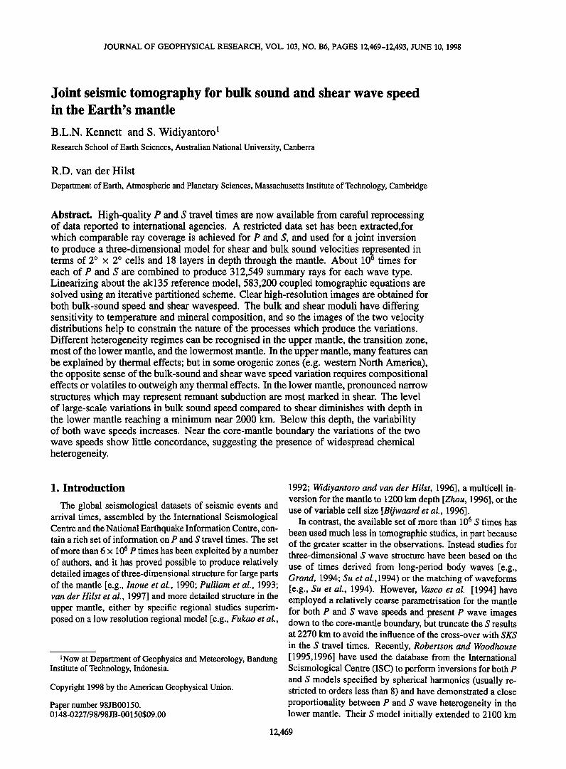
....... '. :ii!ii:i:i:i:i:i:!:: -1.0% +1.0% Figure 5. Inversion of synthetic data with random travel times residuals with a Gaussian distribution and 1 s 2 variance: (a) layer centered at 150 km depth, (b) layer centered at 590 km depth.

tle. As in all travel time tomography we have no access to the variations in density and will therefore have to base our interpretation on just the wave speed heterogeneity.

In terms of the bulk modulus to, shear modulus/x, and density p, the relative variations in the bulk sound speed and shear wave speed can be expressed as

..... (6) qb 2to 2p' /5 2tz 2p

Thus if variations in wave speed are due to density alone, we would expect the relative variations in bulk-sound speed and shear wave speed to be equal.

The variations in P wave speed associated with variations in bulk-sound speed and shear wave speed can be represented as

&c• &p &/• 4/52 (7) = - = where r/varies between 0.42 and 0.375 for plausible P and S velocities for the mantle. The contribution of relative varia-

tions in bulk-sound speed (•iqb/qb) to P heterogeneity is therefore weighted slightly more strongly than the corresponding shear wave speed contribution (•i/3//5). Equation (7) can also be used to recover the equivalent P wave speed distribution from the results of the joint inversion.

If the variations in bulk-sound speed are correlated with the variations in shear wave speed so that they are locally pro- portional, i.e., (,•½/½) = •(•i/3//3), then

ity stations do not report S and so we lose the benefit of their P observations. The recovery in oceanic areas at shallower depth is unfortunately generally rather poor, and Africa re- mains undersampled at all depths.

Nevertheless, as illustrated in Plate 1 in those regions with reasonable ray coverage, the results of the inversion with the restricted ray-coverage and the joint inversion for shear wave speed agree well with the study by Widiyantoro [1997] in which the full available set of S data was supplemented by SKS information (from 84ø-105 ø) to give maximum resolution of SV wave structure.

The stability of the inversion procedure with the 2 ø x 2 ø cellular representation is demonstrated in Figure 5 in which the influence of random noise on the inversion has been sim-

ulated using synthetic data following Grand [ 1994]. A data set with random travel time residuals with a Gaussian prob- ability distribution with zero mean and variance of 1 s 2 has been inverted to give apparent structure. Figure 5 illustrates the situation in the upper mantle and transition zone. The size of the recovered structure from this synthetic data set is small compared to that from the actual inversions, which indicates that there is no introduction of bias owing to the mapping of random errors. This provides additional confidence in the results we present.

2.5. Relations Between Different Measures of

Heterogeneity

The joint inversion provides us with estimates of the variations in the bulk-sound speed and shear wave speed with which we seek to to understand the nature of Earth's man-

= (1 - n) + n], (8) and the local ratio of the heterogeneity in P and S wave speeds becomes

Olnt• *t•/t• ]_• v= = =[•(1-r/)q-r/ . (9)

The ratio v has often been used a proxy for estimating the influence of the bulk modulus from tomographic inversions. Robertson and Woodhouse [ 1995,1996] suggest that for large scale structure (angular order I < 8), v varies between 1:7 at the top of the lower mantle and 2.6 at 2000 km depth. This would require the constant of proportionality •, for these large scales, to vary from 0.29 at the top of the lower mantle to very close to zero at 2000 km. In the finer-grained inversion for bulk-sound and shear heterogeneity we have undertaken, we determine the pattern of bulk-sound variation, and so we can examine the spatial variability Of the ratio • between the bulk-sound and shear heterogeneity and hence also that of v.

The relative variation in the Poisson's ratio &r/or is pro- portional to the difference between the relative variations in bulk modulus and shear modulus,

•cx;: --2 •i/3) = 2•i;[•_1], (10) and so the patterns of variation can be inferred from the wave speed variations and the heterogeneity ratio • (Plates 3-8).


3. Bulk-Sound and Shear Heterogeneity

In order to provide an effective visual presentation of the joint inversion results, we present the heterogeneity patterns for both bulk-sound and shear wave speeds and accompany these with a summary plot of the ratio of deviations of the bulk-sound and shear wave speeds from the reference model (Plates 3-8). To avoid the influence of minor structures in the heterogeneity ratio, we have both excluded deviations < 0.1% for either wave speed and averaged the heterogeneity ratio •' over 6øx 6 ø blocks. These ratio plots are useful for assessing the general character of the heterogeneity, and also highlight those regions in which the behavior of the bulk- sound and shear wave speed is discordant.

3.1. Upper Mantle and Transition Zone

The upper mantle is a zone of significant heterogeneity for seismic wave speeds and this is manifest in both the bulk- sound speed and the shear wave speed. In Plate 6 we present the heterogeneity patterns for both wave speeds for the layer from 100 to 200 km depth, with a common scale for the perturbations from the ak135 reference model, together with the heterogeneity ratio averaged over 6 ø blocks as discussed above.

There are a number of similar features in both the bulk-

sound and shear heterogeneity models. The shields in Aus- tralia, India, and also northern Asia are associated with ele-

vated velocities. The narrow high-velocity anomalies arising from subduction zones, notably in the northwest Pacific and the Tonga-Kermadec zone are distinct in both images. How- ever, these common features are balanced by some very clear differences between the two wave speeds. The mid-ocean ridge system has a modest but distinct signature of lowered velocity in the shear wave speed image. However, there is little indication of the ridges in the bulk sound speed, and where it can be seen, the wave speeds are slightly higher than the reference model (as noted for the East Pacific Rise by Su and Dziewonski [ 1997]). Clearly, nearly all the signal in the P and S wave travel times for events on the mid-ocean

ridge system can be explained by a variation in shear modulus alone in the region of elevated homologous temperature beneath the ridge. Low shear wave speed anomalies are also prominent in a number of backarc settings, such as the Lau Basin near Fiji and behind the Indonesian and Andaman arcs. In the region of subduction in southern Japan, there is a close correspondence between the pattern of heterogeneity in bulk- sound and shear wave speeds.

Two regions where there is a marked difference in the behavior of the two wave speeds are in the orogenic belts ex- tending through southern Europe to Iran and in western North America. In each case, the shear wave speeds are significantly reduced relative to the reference model, whilst the bulk-sound speeds are generally mildly increased. Although there is likely to be a thermal component to the heterogeneity, the differences between the wave speeds would suggest that chemical heterogeneity may well be important in these regions. We note that these regions are also characterized by high attenuation (low Q) which may also contribute to the apparent lowering of S wave speeds.

In the upper mantle many of the zones of lowered wave speed (e.g., around Hawaii, the east African rift, and in backarc settings), show stronger shear deviations as would be expected from a thermal origin. However, the positive deviations of bulk-sound speed from the reference model are somewhat larger than those for shear wave speed, as can been seen in the saturation of the ratio plot at positive values. Such a pattern is not compatible with a purely thermal explanation and suggests that there may well be a compositional component in the dominantly continental zones where such strongly elevated bulk-sound speeds occur.

The differences in western North America between the

bulk-sound and shear wave speeds persist into the transition zone, as can be seen in Plate 4 for the heterogeneity patterns at 465 km. What is happening is that both P and S wave speeds are slower than the reference model, but the perturbation in shear wave speed is larger than is needed to explain the variation in P wave times and so a positive perturbation is required in the bulk-sound speed.

In this depth range at the top of the transition zone, the high velocities associated with subducting slabs show up clearly in the shear wave speed image, particularly in the Tonga- Kermadec, Indonesian-Andaman, and northwest Pacific zones. The correspondence with the bulk-sound variations is somewhat mixed. There is a high-velocity feature associated with the Tonga subduction zone, and the Indonesian arc can be followed to the west along the Andaman arc into Burma.

A striking feature in the bulk-sound image at the top of the transition zone is the well-developed lowered wave speeds bordering the subduction zone structures, e.g., between In- dia and the Andaman arc, which have a partial correspondence with the shear wave image. The mid-ocean ridge structure persists because of vertical smearing associated with the near-vertical ray paths for the events along the ridge axes. In the absence of crossing rays, we cannot attain adequate vertical resolution and so this deep signature is unlikely to be significant.

3.2. Lower Mantle

The nature of the bulk sound and shear wave speed has a distinct change below the transition zone, as the narrow subduction zone anomalies are replaced by broader regions of similar character. This is clearly seen in Plate 5, which illustrates the results of the joint inversion for the layer centered at 740 km. In the shear wave image we can see the high- velocity anomaly associated with the penetration of some material from subduction into the lower mantle; these effects are particularly clear for the Tonga region, near Java in the In- donesian arc, and in South America, where they have previously been revealed by regional P wave inversions [e.g. van der Hilst, 1995; Widiyantoro and van der Hilst, 1996; Eng- dahl et al., 1995]. The pattern of bulk-sound variation has a general correspondence to the shear wave results, but there are some notable differences. The region from Tonga across to New Guinea displays a suffused zone of high bulk-sound speeds with only a partial correlation to the shear wave results. Fairly strong bulk-sound speed anomalies occur near southern Japan and Korea that are likely to be related to for-

KENNETT ET AL.: JOINT BULK SOUND AND SHEAR TOMOGRAPHY 12,481

Bulk-sound Layer: 2 100. - 200. km

:- '": .i

Perturbation [%] Ratio

-1.00 0 1.00 -1.50 0 1.50 -1.00 1.00

Plate 3. Results ofjoint inversion for the layer from 100 to 200 km depth, displayed relative to the ak135 reference model (a) bulk-sound speed heterogeneity, (b) shear wave speed heterogeneity, and (c) ratio of bulk-sound to shear heterogeneity averaged over 6øx 6 ø zones.


Layer: 5 410. - 520. km

Bulk-sound • •••--••_____• ••

,

Shear

Ratio

Perturbation [%]

I

-1.00 o 1.00

-1.00 1.00

Ratio

-1.50 0 1.50

Plate 4. Results of joint inversion for the layer from 410 to 520 km depth, displayed relative to the ak135 reference model (a) bulk-sound speed heterogeneity, (b) shear wave speed heterogeneity, and (c) ratio of bulk-sound to shear heterogeneity averaged over 6 ø x6 ø zones.

KENNETr ET AL.: JOINT BULK SOUND AND SHEAR TOMOGRAPHY 12,483

Layer: 7 Bulk-sound •,0. -820. km

o

Shear

••,•:•:•,.•,•,..•:'...•-•-• :,•.. { •. .! ,•, •', ..• ..• .• _ ... • •-

Ratio


I I ............ I ........... I -1.00 0 1.00 -1.50 0 -1.00 1.00

1.50

Plate 5. Results of joint inversion for the layer from 660 to 820 km depth, displayed relative to the ak135 reference model (a) bulk-sound speed heterogeneity, (b) shear wave speed heterogeneity, and (c) ratio of bulk-sound to shear heterogeneity averaged over 6 ø x6 ø zones.


Layer: 10 Bulk-sound •20o. - 1400. km

Ratio


-1.00 0 1.00 -1.50 0 1.50 -1.00 1.00

Plate 6. Results of joint inversion for the layer from 1200 to 1400 km depth, displayed relative to the ak135 reference model (a) bulk-sound speed heterogeneity, (b) shear wave speed heterogeneity, and (c) ratio • of bulk-sound to shear heterogeneity averaged over 6øx 6 ø zones.


mer slab material; however, these features are not as well de-

veloped in the shear wave image. In North America, an interesting separation develops be-

tween a distinct zone of lowered shear wave speeds in the west and higher bulk-sound speeds in the east. The perturbations are not large but are consistent over a broad area. Another region with discrepant patterns in bulk-sound and shear wave speed behavior is evident beneath western Aus- tralia and adjacent parts of the Indian Ocean. This anomaly appears in the transition zone and persists through much of the lower mantle; unfortunately, with the available data coverage the spatial extent of the structure is not well resolved.

In this layer at the top of the lower mantle, the bulk-sound speed heterogeneity is generally somewhat smaller than the equivalent shear heterogeneity. When we allow for the zones where the variations in the two wave speeds have opposite sense, we see that that broad scale averages would be consistent with the estimate of a proportionality factor of 0.29 that we have derived above from the work of Robertson and

Woodhouse [ 1995,1996] on large-scale variation. However, this single value does not adequately characterize the fairly complex pattern of behavior revealed in the joint inversion.

In the depth range from 900 to 1500 km in the lower mantle, prominent relatively narrow zones of high-velocity material become apparent in the Americas and southern Eurasia. These have been recognized previously in separate P and S wave inversions [e.g., van der Hilst et al., 1997; Grand et al., 1997] and have been associated with the relicts of former subduction of the Farallon plate in the Americas [Grand, 1994] and at the northern edge of the Tethys [van der Hilst et al., 1997]. These features can be seen quite well in Plate 6, in the shear wave speed perturbation at 1300 km depth. How- ever, these high-velocity zones have a muted presence in the bulk-sound variation, which at this depth seems to be less or- ganized than the shear wave speed pattern.

The amplitude of the bulk-sound speed variations steadily diminishes as the depth into the lower mantle increases. As a result we have to be careful about placing too much attention on small deviations from the reference model (since they could be model dependent).

At still greater depth between 1900 and 2200 km, the over- all amplitude of the bulk-sound speed variations becomes quite low even though there are noticeable perturbations in the shear wave speed, as can be seen in the results of the joint inversion at 2100 km in Plate 7. The pattern of the ratio of bulk-sound and shear wave speed variation shows a few patches where the size of the ratio is close to unity, but these are associated with very small deviations from the reference. The very low level of the bulk-sound speed variations in the zones of significant shear wave speed heterogeneity supports the inferences that we have made above from the results of Robertson and Woodhouse [ 1996], namely, that near 2000 km the ratio of P to S wave speed perturbations on large scales is such that the bulk-sound speed variations would be a very small fraction of the shear wave speed variations.

Below 2100 km we are still able to extract shear wave

speed images by exploiting the reprocessed arrival time data, which achieve good association of S out to 105 ø (avoiding

the SKS cross-over). Resolution for SV wave structure is enhanced by including SKS from 84 ø- 105 ø [Widiyantoro, 1997]. As the depth increases, the deviations from the reference model become more marked for both the bulk-sound speed and the shear wave speed, as can be seen in Plate 8 for the results of the joint inversion for the layer centered on 2675 km depth.

The disjunction between the bulk-sound speed and shear wave speed variations in the lowermost mantle, which can be very clearly seen in the Plate 8c, is strongly suggestive of widespread chemical heterogeneity. Note that the regions with positive correlation between the two wave speeds are generally associated with very low amplitude of shear wave speed deviations from the reference. The change in the character of the heterogeneity between the middle of the lower mantle and the lowermost part has been pointed out previously, e.g., by van der Hilst et al. [1997] with a tentative association with a lower mantle transition zone in the depth range 1800-2300 km. We note that our joint inversion results are consistent with a significant reorganization of the heterogeneity patterns with depth, passing through a zone with almost no bulk-sound variation to one at the base of the mantle

in which the shear wave speed and bulk-sound speed show little correspondence.

4. Discussion and Conclusions

The images of the variation of bulk-sound speed and shear wave speed that we have been able to produce from the data- set of arrival times for common P and S source/receiver pairs provide a useful complement to previous studies of P and S heterogeneity in the mantle. We are able to begin to separate the contributions of compressibility and shear modulus to the patterns of three-dimensional heterogeneity. The study has been made feasible by the quality of the reprocessed arrival time data set that we have employed [Engdahl et al., 1998].

In those regions with adequate data coverage, we are able to extract good images of the heterogeneity for both wave speeds. Although it is difficult to judge the absolute level of the wave speed perturbations, the relative amplitude of the bulk-sound and shear wave speed models in the joint inversion should be reliable because they have been constructed from P and S data with very similar ray paths.

The patterns of behavior for bulk-sound speed and shear wave speed that we have discussed are in good general agreement with the results presented by Su and Dziewonski [ 1997]. However, the cellular inversion enables us to achieve rather

higher resolution of the varied features in the upper part of the mantle. From the variations in bulk-sound speed and shear wave speed we are able to reconstruct the variation in P wave speed using (7). In those regions where there is good data coverage in the joint inversion, the geographic patterns of variation agree well with those presented by van der Hilst et al. [1997] but the amplitude of variation is about 60% of that achieved in the inversion of the full P wave data set.

For S there is again good agreement in the patterns of variation with the results of Grand et al. [1997] for most of the mantle, with some differences as the core-mantle boundary is approached. The data set of SH wave picks employed by

12,486 KENNETY ET AL.' JOINT BULK SOUND AND SHEAR TOMOGRAPHY

Grand et al. [1997] includes core reflections and their mul- tiples; whereas we have augmented refracted S data with a small number of SKS times which reflect SV structure.

4.1. Summary Variations

In Figure 6a we display the RMS variations in the relative wave speed perturbations for bulk-sound speed, shear wave speed, and P wave speed (reconstituted from equation (7)) as a function of depth through the 18 layers employed in the inversion. The variations have been weighted by the sampling

The summary values displayed in Figure 6a do not tell the whole story, because as we have seen the character of the bulk-sound and shear wave perturbations evolve with depth, and there is significant lateral variation at all depths. Near 2000 km, the bulk sound variation is distributed in relatively large scale features of both signs so that broad-scale averages are low. Below 2000 km, both bulk-sound and shear varia-

tions tend to increase significantly. As in a wide-variety of other studies, we find that the variation near the core-mantle

boundary tends to approach levels comparable to the upper

in the mantle to try to minimize the influence of the varia- mantle. The influence of the cross-over between S and SKS tions in path coverage. As we have noted above, the level of reduces the available sampling of the lowermost mantle. shear perturbation at shallow levels is almost certainly under- The corresponding RMS values of the two ratios of hetero- estimated because of the geographic distribution of stations reporting S and the curtailment of large residuals in the inversion. With the available data set of P and S along comparable paths the levels of bulk-sound and shear variation are similar in layers 1-3 (0-300 km) and thereafter the shear variation is larger, usually by 30% or more. The RMS relative variations in P wave speed are slightly smaller than for either bulk- sound or shear wave speed and reflect the interaction of the contributions from the bulk and shear moduli.

0.6

(a)

0.5

0.4

0.3

0.2 0.1

0.0

2.5

(b)

2.0

1.5

1.0

0.5

0.0

I I I I I

I I I I I

500. 1000. 1500. 2000. 2500.

Depth [km]

I I I I I

i i

500. 1000.

I

1500.

Depth [km]

I

2500.

geneity •' and v are displayed in Figure 6b as a function of depth for the 18 layers. Once again the variations have been weighted by the sampling in the mantle to try to minimize the influence of the variations in path coverage. The ratio •' between the relative variations in bulk-sound and shear wave

speeds has been displayed as a function of position in Plates 3-8, and we note there is significant variability. Nevertheless, for much of the midmantle the RMS value of • is close to 0.6 which is similar to the results derived from splitting of normal mode multiplets for much lower frequencies (J. Tromp, personal communication, 1997). As the core-mantle boundary is approached, the RMS value of • increases, but as we have noted previously, in this region there are contributions from features with both positive and negative values of •' (see Plate 8). The RMS value of v, the ratio of the logarithmic derivatives of S and P variations, is close to a constant value

of 2.1 throughout the lower mantle. The restricted choice of paths may well contribute to muted results in the lower mantle where other studies have indicated a rise in the value of

v. Even though the preferred model of Robertson and Wood- house [ 1996] for a global value of v derived from spherical harmonic analysis rises from 1.9 at the top of the lower mantle to 2.5 at 2000 km depth, the error bars on the individual depth estimates would not preclude a nearly constant value.

Figure 6. (a) The RMS variation of the relative perturbation in bulk-sound speed •iqS/qS, shear wave speed t515/15 and P wave speed •ic•/c• as a function of depth, weighted by the sampling of the mantle. (b) The RMS values of the ratio •' between bulk and shear wave speed variations and the ratio v between shear and P wave speed variations as a function of depth, again weighted by the sampling of the mantle

4.2. Patterns of Heterogeneity

From the models for the three-dimensional heterogeneity in both bulk-sound and shear wave speeds, we can recognize

- substantial differences in the heterogeneity regimes in different parts of the Earth, although detailed interpretation of the

_ patterns may be difficult. In the upper mantle and transition zone, the major subduction zones can be clearly followed in the shear wave speed distribution (even though we were not

- using the full available S arrival time set), but have a somewhat patchy character in the bulk-sound images. The nature of the subduction processes revealed in these images agrees

3000. well with previous results from regional and global P wave studies.

In the upper mantle, the bulk-sound variations, particularly in stable continental zones, are stronger than the shear wave speed variations which may suggest some compositional component (compare the tectosphere hypothesis [Jor- dan 1975, 1978]). There are other regions (e.g., Hawaii and the east African rift) where there is a close correspondence

KENNET'[' ET AL.: JOINT BULK SOUND AND SHEAR TOMOGRAPHY 12,487

between the patterns of heterogeneity but with larger shear the north by a distinct high wave speed feature. The stronger variation which is consistent with elevated temperature. bulk-sound speed variations suggest that there may be a com- However, in the orogenic belts in western North America positional component to the heterogeneity. and southern Europe to Iran the shear perturbations are larger than are required to explain the P wave delay times, which suggests the presence of some component of chemical heterogeneity or the influence of volatiles.

As the depth increases in the lower mantle, the correlation between the bulk-sound speed variation and the distribution of shear wave speeds diminishes. Near 2000 km depth, there is only a modest contribution from the bulk modulus, and the patterns of bulk-sound speed and shear wave speed reveal very little broad scale correspondence. The spherical harmonic representations of bulk sound and shear velocity presented by Su and Dziewonski [ 1997] show a somewhat higher contribution from bulk-sound in the upper part of the mantle. However, as noted above, the weak large-scale contribution from bulk-sound near 2000 km depth is consistent with the work of Robertson and Woodhouse [ 1995,1996] using travel time information.

At even greater depths in the lowermost mantle, the size of the perturbations in both wave speeds increases, but the patterns are relatively distinct. This divergent behavior between the wave speed distributions suggests that the lowermost 800-900 km is characterized by the presence of widespread chemical heterogeneity which may well comprise some of the distinct chemical reservoirs required to satisfy isotope data. Such chemical heterogeneity could survive at the base of the mantle as a result of incomplete mixing in the high-viscosity lower mantle (as first suggested by Davies, [1977, 1984]). The presence of small bodies of chemically distinct material in the lowermost mantle is also suggested from studies of scattering of high-frequency body waves such as PKP [Hedlin et al., 1997]. The increased levels of variation and the discordant behavior of the bulk-sound and shear

velocities near the core-mantle boundary are also a feature of the models of Su and Dziewonski [1997], who provide ther- modynamic arguments for at least a partial thermal contribution.

Many of the features of the heterogeneity regimes in the mantle are well illustrated by a cross section through the bulk- sound and shear wave speed distributions along a great circle whose normal lies at 24øW, 7øN (Plate 9). The path covers a wide range of surface tectonic environments cutting through southwestern Australia, the Banda Sea, south China, and

northern Eurasia and then passing to the east of the North American coastline and through the South American conti- nent, where the cross section intersects with the eastward dipping slab of former Nazca and Farallon ocean floor.

The relatively narrow subduction zone dipping beneath the Banda Sea, which can be seen in both shear and bulk sound, thickens into the lower mantle and then grades into an extended structure in middle mantle which forms part of the

The section also cuts into the narrow feature in the mid-

mantle beneath the Americas, which is also most pronounced in shear. There is a significant three-dimensional effect in the cut through an easterly dipping structure, but the weak signature in shallow structure arises in part from low station density in this region. The apparent contrast between the bland structures in the southern hemisphere and the more complex patterns in the north is also related to the limited resolution attainable in southern latitudes with the present data coverage.

Beneath the Eurasian region in the lower mantle, we can see the general trend of a diminishing amplitude of bulk- sound variation compared to shear as depth increases with the lowest amplitude near 2000 km depth. Beneath this depth the heterogeneity in both bulk sound and shear can be seen to increase but with only partial correspondence in the patterns of variation.

The three-dimensional models of wave speed variation we have presented have been derived by a linearized inversion around the ak135 radial model. The presence of zones of large scale systematic deviation from the reference model, e.g., the very fast shield zones in the uppermost mantle indicates that we may well be reaching the limits of linearized analysis in the joint inversion. To stay within the lineariza- tion limit in the next generation of models is likely to require a three-dimensional reference model, at least in the upper mantle, and three-dimensional ray tracing on updated models, which would be a major task even for the 300,000 summary rays for each wave type employed in the present study.

Appendix A: Structural Recovery From P and S Travel Times

From the global database we have observations of P and S arrival times at a large number of stations and, once we have a suitable hypocenter estimate, can derive travel times t• and ts. From seismic ray theory we can represent the P travel time for the i th observation as

tPi : = ds a(r), (A1) ay• o•(r) ay•

in terms of the P wave speed o•(r) and the P wave slowness a(r) = 1/o•(r). The jth S travel time is represented by the ray path integral

fr dS fr ds b(r), (A2) tsj= ayj/•) = ayj in terms of the S wave speed/• (r) and the S wave slowness b (r) = 1/fi (r).

We undertake a joint inversion for bulk-sound speed •p and elongate feature along the southern margin of Asia in the shear wave speed • from the reported travel times for more depth range from 1000 to 1400 km. There is only a weak than 35,000 seismic events with comparable ray paths for indication of a bulk-sound feature in the lower mantle. In both P and S. so that we can combine the the two classes of

the upper mantle transition zone, there is a strong zone of re- information. We will work in terms of slowness because the duced bulk-sound speed below southern China bordered to Frdchet derivatives of the travel times take a much simpler


form, and we represent the P wave slowness a(r) in terms of the shear slowness b(r) and the bulk-sound slowness c(r) = 1/½(r).

As discussed in the text, we make the assumption that the hypocenters of events are sufficiently well known that we can work directly with the travel times for P and S waves. The global travel-time data we employ have been extensively reprocessed by Engdahl et al. [1998], and the relocated hypocenters from this work are significantly improved from the original catalogues.

We introduce a partitioned data vector of observed travel times

d = (t•, ts) T (A3)

and a corresponding set of theoretical times

do = (tr0, ts0) T (A4)

derived from the current model of three-dimensional bulk

sound and shear structure.

As a measure of data fit including both P and S travel times we employ

7v• = (d - d0)•C• • (d - do), (AS)

where we partition the data covariance matrix

C•I = 0 C• (A6)

P+Pm

(d - do)rC•l(d - do) +•' (m - mo)•D(m - mo)

+(m too) • -• -- Cm (m -- mo) , (AlO)

where the data are regarded as functionals of the model parameters and >, is a variable weighting for gradient smoothing. We expand 7 v about the reference model to quadratic terms in the model perturbation Am = m -- m0

1

P = 7V(mo) + 0 • Am + • Am•HAm + .... (All)

In terms of the misfit Ad between the observed travel times d

and the values from the reference model do, the gradient with respect to the model parameters

0 = G•C• • Ad, (A12)

where the Fr6chet derivative matrix G and the Hessian matrix

H are given by

O d H -- G r c • ' G .-JF •mm mo G= mo ' Ad+ },D+C•, 1.

(A13)

For a minimum with respect to the model perturbation Am we require the model perturbation to be found from

o + HAm = 0, (A14)

since the P travel times and S travel times can be plausibly as- sumed to be independent (weak dependence may arise through the hypocenter location).

We represent the model also by a partitioned vector in model space

m = (c, b) T, (A7)

where c are the bulk-sound slowness parameters and b are the shear slowness parameters.

We impose a smoothness constraint on both the shear and bulk-sound slownesses by using a first order difference op- erator D, which will be represented by a quadratic form in model space and also a model norm constraint using a model covariance matrix Cm

7v m y (m_mo) •D(m_mo) + (m_mo) • -1 = C m (m-mo), (A8)

where mo represents the values for the reference model ak135 [Kennett et al., 1995]. The model covariance term

C ;n• = ( C c-cl C c-• ) (A9) Cb- • -• , Cbb

for which a formal solution for Am can be produced through the action of a generalised inverse H-.

In terms of the data partition between P and S travel times,

O= (Oc)=GrG•iAd=G r (C•p 0 O• 0 Cj} At s ' (A15)

with a corresponding partition of the Fr&het derivative matrix G in terms of the bulk sound and shear slownesses

G = ( 0 Ate/Oc 0 OAte/Ob)=(Gec OAts/Ob 0 Geb ) . (A16) Gsb

The partial derivatives of the P wave times with respect to the bulk sound and shear slowness can be obtained by a simple scaling of the derivative with respect to P slowness,

tStpi = fray, fr ( a3 4a3 ds 8a = ds •-5-8c + •-5-8b) . ay,

The partitioned form of the gradient vector is

and we anticipate that Cc•, Cb-c • will be much smaller than Cc•, Co-•. In order to apply a weak cross-wave speed regularization in the joint inversion have taken the off-diagonal partitions to be a factor of 50 smaller than the diagonal partitions of C•7/1 ß

In order to extract the three-dimensional structure specified by the model vector m we now seek to minimize a com- bination of the data fit and model regularization terms

(Oc) ( G•,cC•Ate 0 = O• = G½•C•eAte +G•bC•At s ' (A17)

and, neglecting second-order terms, the Hessian matrix takes the partitioned form

Hcc Hcb) (A18) H= Ht, c Ht, t,

KENNETT ET AL.: JOINT BULK SOUND AND SHEAR TOMOGRAPHY 12,489

Layer: 14 Bulk-sound _ .... • 2000. - 2200. km

Shear _ _ • •.. ••

.•'


-1.00 0 1.00 -1.50 0 1.50 -1.00 1.00

Plate 7. Results of joint inversion for the layer from 2000 to 2200 km depth, displayed relative to the ak135 reference model (a) bulk-sound speed heterogeneity, (b) shear wave speed heterogeneity, and (c) ratio • of bulk-sound to shear heterogeneity averaged over 6øx 6 ø zones.


•Layer: 17 600. -2750. km Bulk-sound _--

Shear

'- • •'• - -• ---• --i

,/'• • •'•, . L •• •_ '•

,..

Ratio


-1.00

-1.00

i i i ii

0 1.00 -1.50 0 1.00

1.50

Plate 8. Results of joint inversion for the layer from 2600 to 2750 km depth, displayed relative to the ak135 reference model (a) bulk-sound speed heterogeneity, (b) shear wave speed heterogeneity, and (c) ratio •' of bulk-sound to shear heterogeneity averaged over 6øx 6 ø zones.

KENNETT ET AL.' JOINT BULK SOUND AND SHEAR TOMOGRAPHY 12,491

• o

o o

o o

o '• • o

o

12,492 KENNET'F ET AL.: JOINT BULK SOUND AND SHEAR TOMOGRAPHY

where

cc

Hc•

Hbc

Hbb

ecC•Xe G ec + Y Dcc + Ccc, = G r -1 ecC•Xe G eb + Ccb,

T -1 -1

= G?bC??G?c + Cbc, T -1 T -1

= Gst, Css st, GpbCppGpb + G + YDbb + Cb- •. (A19)

By working with both P and S travel times simultaneously, we are faced with having to solve a very large set of approximately 600,000 linear equations to determine three-dimensional structure. Fortunately we can exploit the partitioned character of (A17), (A18) above to produce an efficient iterative scheme, which is developed in Appendix B. In this iterative scheme, we solve sequentially for bulk-sound and shear wave speeds and introduce cross correction terms between the two partial inversions. Since we only use half the equations at a time, the computational load is significantly reduced.

We now make use of the partitioned gradient vectors Oc, Ob derived from the P and S travel time residuals which express

(cc Hbc Hbb b Ob '

where we anticipate that the major contributions will come from the block diagonal elements Hcc, Hbb. The formal inverse of the Hessian matrix can be written in the form

Hcc Hcb = I H•-c • Hcb H•-c • 0 Hbc Hbb Hb½Hbc I 0 Hb• '

(•)

and then we can expand the matrix inverse on the right hand side in successive powers of the off-diagonal elements to yield

( ) 1 ( ) Ucc -= o

_( o u; )

(•3)

the separation of the dependence on bulk sound and shear We can now construct a series of approximations for the vec- slowness. The rth iteration for the bulk soundandshearslow- tors c, b by using the successive terms in (B3). The initial ness in the three-dimensional model then takes the form

Cr '-- H•-c•(-Oc- Hcbbr-1), (A20) br = Hb• (--Ob - HbcCr-1),

with cross-corrections from the solutions of the previous (r- 1)th iteration. The iteration sequence is initiated without including any cross-terms

Co = -H•-c•Oc, (A21) = --HbbO b.

In effect, each successive iteration aims to work with a vector on the right-hand side of the equations which represents just the contribution from a single wave type by correcting for the influence of the other wave type.

In the application of (A20) and (A21) the inverses of the diagonal blocks of the Hessian matrix represent the solution of the corresponding sets of linear equations, e.g.,

Hcccr = -Oc- Hcbbr-1,

which is accomplished using a biconjugate gradient procedure LINBCG, [Press et al., 1992]. The iteration proceeds with a sequence of solutions of the same linear equations with different right-hand sides and the off-diagonal blocks of the Hessian are not involved in the solution of the linear equations.

This procedure has proved to be both effective and conve- nient, for a reasonably fine parametrization of three-dimensional structure, and brings the very large system of equations (A14) within the scope of a powerful workstation.

Appendix B: Inversion of Coupled Linear Equations

We can write the equations (A14) to be solved for the joint tomography problem in the form

expressions ignore the off-diagonal terms

Co = -H•c•Oc, (B4) b0 =

and then we introduce correction terms to compensate for the cross-coupling between the sets of equations

c• = •;i (-Oc - •tc• •ti; o •) = •tZc • (-Oc - •tc• b0), bl = Hl• • (--Ob -- HbcH•c•Oc) = H[• (--Ob -- Hbc½O).

(B5)

The second iteration appears to be a little more complex,

c2 = H•-c'(-Oc- HcbbO + HcbH[•H•cH•-c•Oc), b2 = H[• (--Oh -- HbcCO + Hb c H•-c • Hcb H•-c•Ob),

(B6)

but after some manipulation, we find

c2 = H•c • (-Oc - Hcbbl ), b2 = Ht• (--Ob - HbcCl ).

(B7)

A similar pattern emerges for the higher-order corrections and so we obtain an iterative update for the structure vectors c, b as

Cr •-- Hgc • (Oc - Hcobr-1 ), (B 8) br = Hb• (Oh -- HbcCr-1 ).

In a practical sense, H[c •, H[• represent the solution of partial sets of the linear equations and the coupling is introduced by successive modifications of the right hand sides of the equations. The iteration scheme (B8) is equivalent to a partitioned form of a Jacobi algorithm.

Acknowledgments. The quality of tomographic images obtained in this study owes much to the efforts of Bob Engdahl in refining traveltime information, particularly in the reprocessing of multiple data sets. B.L.N.K would like to thank the Earthquake Research Institute, University of Tokyo, for support from the cooperative research program (1997-VI-02) during the writing of much of the paper. R.v.d.H. acknowledges support by NSF Grant

KENNET'F ET AL.: JOINT BULK SOUND AND SHEAR TOMOGRAPHY 12,493

EAR-9628087. S.W. was supported by an AusAid Ph.D. Scholar- ship at the Research School of Earth Sciences, Asutralian National University, while on leave from the Department of Geophysics and Meteorology, Bandung Institute of Technology, Indonesia.

References

Bijwaard, H., W. Spakman, and E.R. Engdahl, High resolution global delay time tomography, Eos Trans. AGU, 77(46), Fall Meet. Suppl., 1482, 1996.

Davies, G.F, Whole mantle convection and plate tectonics, Geo- phys. J. R. Astron. Soc., 49, 459-486, 1977.

Davies, G.F, Geophysical and isotopic constraints on mantle convection: An interim synthesis, J. Geophys. Res., 89, 6017-6040, 1984.

Dziewonski, A.M., and D.L. Anderson, Preliminary reference Earth model, Phys. Earth Planet. Inter., 25, 297-356, 1981.

Engdahl, E.R., R.D. van der Hilst and J. Betfocal, Imaging of subducted lithosphere beneath South America, Geophys. Res. Lett., 22, 2317-2330, 1995.

Engdahl, E.R., R.D. van der Hilst and R. Buland, Global teleseismic earthquake relocation with improved travel times and procedures for depth determination, Bull. Seisin. Soc. Am., in press, 1998.

Fukao Y., M. Obayashi, H. Inoue, and M. Nenbai, Subducting slabs stagnant in the transition zone, J. Geophys. Res., 97, 2809-4822, 1992.

Grand, S.P., Mantle shear structure beneath the Americas and

sions for mantle P wave velocity structure based on the minimiz- ation of •2 and • norms of International Seismological Centre travel time residuals, J. Geophys. Res., 98, 699-734, 1993.

Robertson, G.S., and J.H. Woodhouse, Evidence for the proportionality of P and S heterogeneity in the mantle, Geophys. J. Int., 123, 85-116, 1995.

Robertson, G.S., and J.H. Woodhouse, Ratio of relative S to P velocity heterogeneities in the lower mantle, J. Geophys. Res, 101, 20,041-20,052, 1996.

Su, W.-J., and A.M. Dziewonski, Simultaneous inversion for 3D variations in shear and bulk velocity in the mantle, Phys. Earth Planet. Inter., 100, 135-156, 1997.

Su, W.-J., R.L. Woodward, and A.M. Dziewonski, Degree-12 model of shear velocity heterogeneity in the mantle, J. Geophys. Res., 99, 6945-6980, 1994.

Tan B., I. Jackson, and J. Fitz Gerald, Shear wave dispersion and attenuation in fine-grained synthetic olivine aggregates: Prelim- inary results, Geophys. Res. Lett., 24, 1055-1058, 1997.

van der Hilst, R.D., Complex morphology of subducted lithosphere in the mantle beneath the Tonga trench, Nature, 361,699-704, 1995.

van der Hilst, R.D., S. Widiyantoro, and E.R. Engdahl, Evidence for deep mantle circulation from global tomography, Nature, 386, 578-584, 1997.

Vasco, D.W., L.R. Johnson, R.J. Pulliam, and P.S. Earle, Robust inversion of IASP91 travel time residuals for mantle P and S

structure, earthquake mislocations, and station corrections, J. Geo- surrounding oceans, J. Geophys. Res., 99, 11 591-11 621, 1994. phys. Res., 99, 13,727-13,755, 1994.

Grand, S.P, R.D. van der Hilst, and S. Widiyantoro, Global seismic Widiyantoro, S., Studies of seismic tomography on regional and tomography: A snapshot of convection in the Earth, GSA Today, global Scale, Ph.D. thesis, Aust. Natl Univ., Canberra, 1997. 7(4), 1-7, 1997.

Hedlin, M., P. Shearer, and P.S, Earle, Waveform stacks of PKP precursors: Evidence for small-scale heterogeneity throughout the mantle, Nature, 387, 145-150, 1997.

Inoue, H., Y. Fukao, K. Tanabe, and Y. Ogata, Whole mantle P-wave travel time tomography, Phys. Earth Planet. Inter., 59, 294-328, 1990.

Jordan, T.H., The continental tectosphere, Rev. Geophys., 13, 1-12, 1975.

Jordan, T.H., Composition and development of the continental tectosphere, Nature, 274, 544-548, 1978.

Kennett, B.L.N., E.R. Engdahl, and R. Buland, Constraints on seismic velocities in the Earth from travel times, Geophys. J. Int., 122, 108-124, 1995.

Nolet, G., Seismic wave propagation and seismic tomography,, in Seismic Tomography, edited by G. Nolet, pp 1-23, D. Reidel,

Widiyantoro, S., and R.D. van der Hilst, Structure and evolution of lithospheric slab beneath the Sunda arc, Indonesia, Science, 271, 1566-1570, 1996.

Wysession, M.E., L. Bartk6, and J.B. Wilson, Mapping the the lowermost mantle using core-reflected shear waves, J. Geophys. Res., 99, 13 667-13 684, 1994.

Zhou, H.-W., A high resolution P wave model for the top 1200 km of the mantle, J. Geophys. Res., 101, 27791-27 810, 1996.

B. L. N. Kennett, Research School of Earth Sciences, Australian National University, Canberra ACT 0200, Australia. (e-mail: brian @rses.anu.edu.au)

R.D. van der Hilst, Department of Earth, Atmospheric and Planetary Sciences, Massachusetts Institute of Technology, Rm 54-514, Cambridge MA 02139-4307. (e-mail: [email protected])

S. Widiyantoro, Department of Geophysics and Meteorology, Norwell, Mass., 1990. Bandung Institute of Technology, J1. Ganesa 10, Bandung, 40132,

Press, W., B.P. Flannery, S.A. Tuekolsky and W.T. Vetterling, Nu- Indonesia, (e-mail: [email protected]) merical Recipes in FORTRAN, 2nd ed., Cambridge Univ. Press, New York, 1992. (Received July 14, 1997; revised December 12, 1997;

Puliiam, R.J., D.W. Vasco and L.R. Johnson, Tomographic inver- accepted January 7, 1998.)

joint seismic tomography for bulk sound and shear wave...

Documents