slide 1

Slide 1

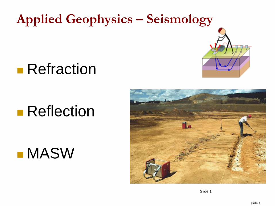
Applied Geophysics – Seismology

Refraction

Reflection

MASW

slide 2

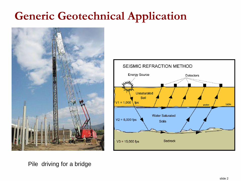
Generic Geotechnical Application

Pile driving for a bridge

slide 3

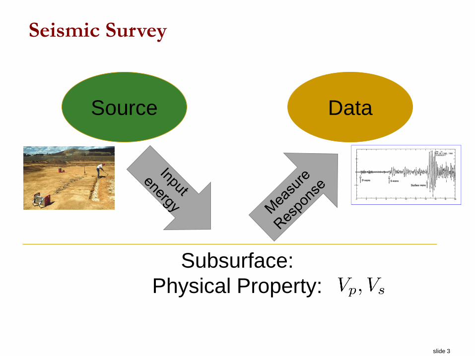
Subsurface:

Physical Property:

Source Data

Seismic Survey

slide 4

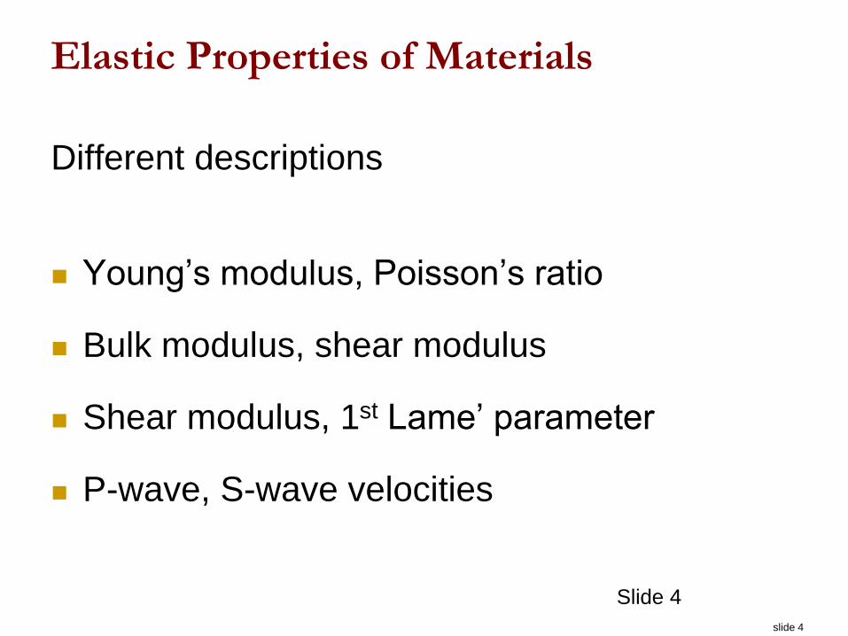
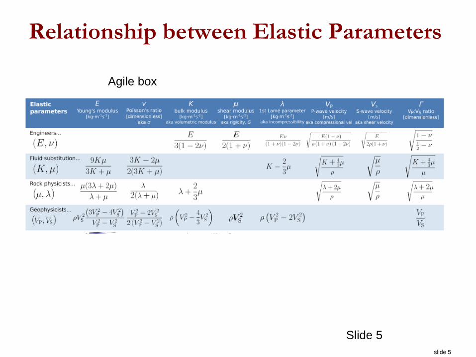
Elastic Properties of Materials

Different descriptions

Young’s modulus, Poisson’s ratio

Bulk modulus, shear modulus

Shear modulus, 1st Lame’ parameter

P-wave, S-wave velocities

Slide 4

slide 5

Relationship between Elastic Parameters

Slide 5

Agile box

slide 6

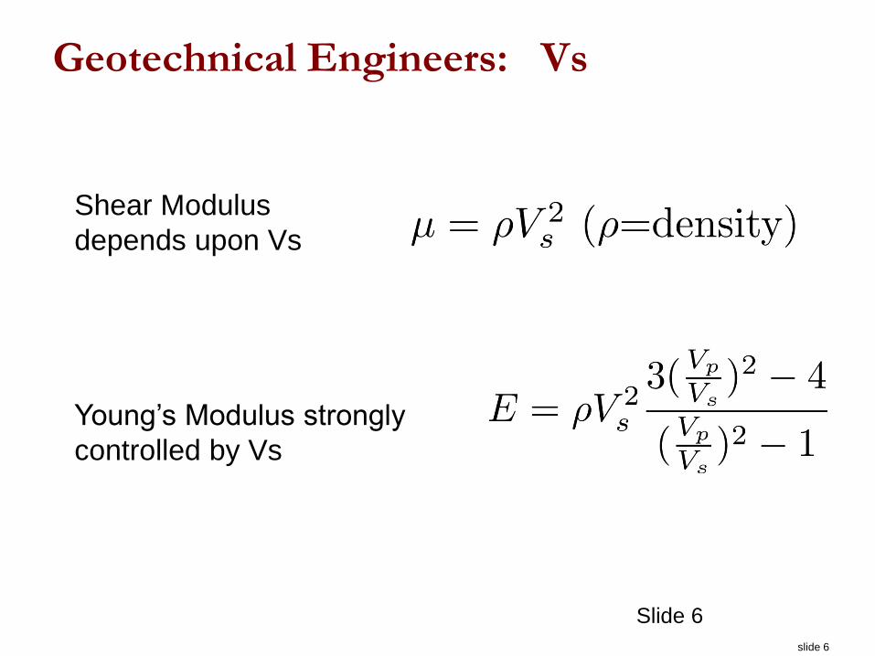
Geotechnical Engineers: Vs

Slide 6

Shear Modulus

depends upon Vs

Young’s Modulus strongly

controlled by Vs

slide 7

Elastic properties

GPG: elastic properties

Slide 7

slide 8

Subsurface:

Physical Property:

Source Data

Seismic Survey

slide 9

Slide 9

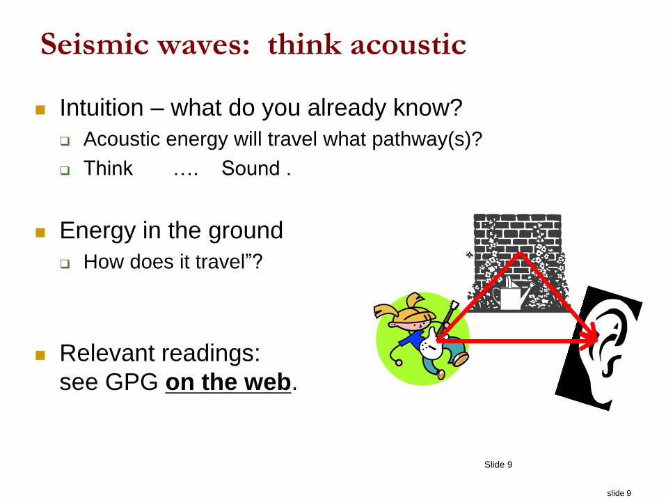
Seismic waves: think acoustic

Intuition – what do you already know?

Acoustic energy will travel what pathway(s)?

Think …. Sound .

Energy in the ground

How does it travel”?

Relevant readings:

see GPG on the web.

slide 10

Slide 10

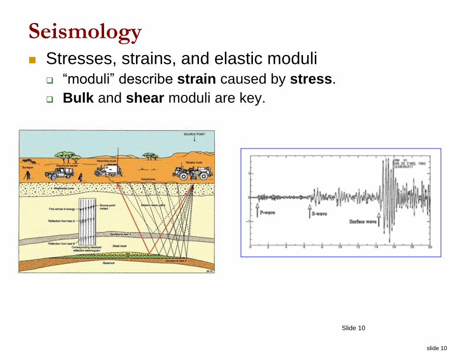
Seismology Stresses, strains, and elastic moduli

“moduli” describe strain caused by stress.

Bulk and shear moduli are key.

slide 11

Slide 11

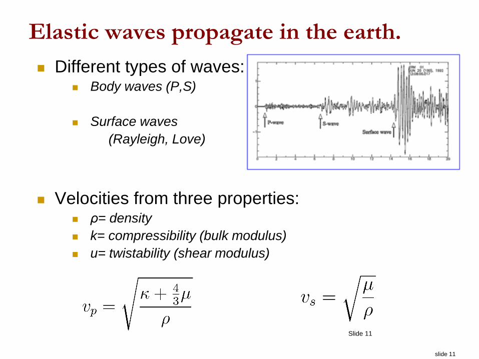
Elastic waves propagate in the earth.

Different types of waves: Body waves (P,S)

Surface waves

(Rayleigh, Love)

Velocities from three properties: ρ= density

k= compressibility (bulk modulus)

u= twistability (shear modulus)

slide 12

Student Participation

Seismic waves propagating along a line of

students

GPG: Basic principles

Waves

Ray paths

Attenuation

Slide 12

slide 13

Slide 13

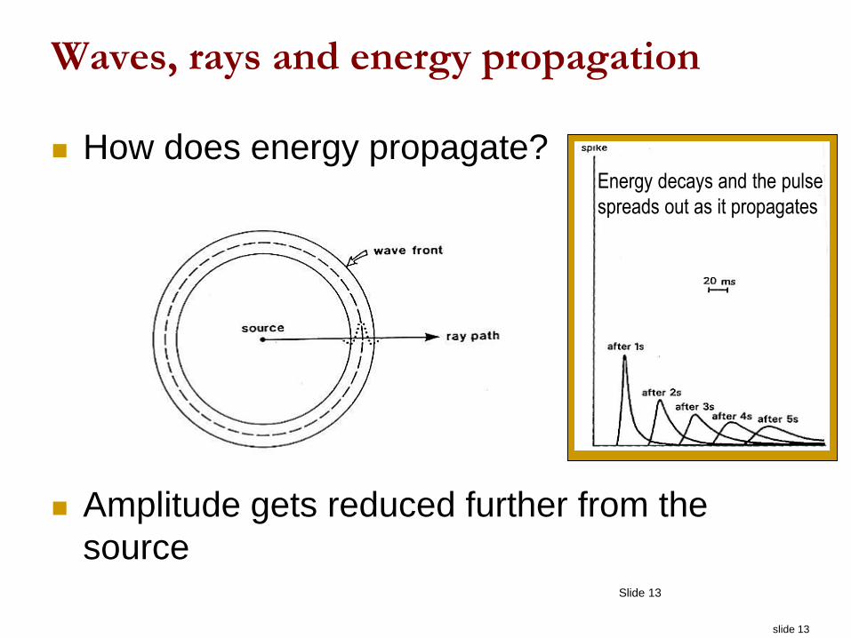
Waves, rays and energy propagation

How does energy propagate?

Amplitude gets reduced further from the

source

Energy decays and the pulse

spreads out as it propagates

slide 14

Slide 14

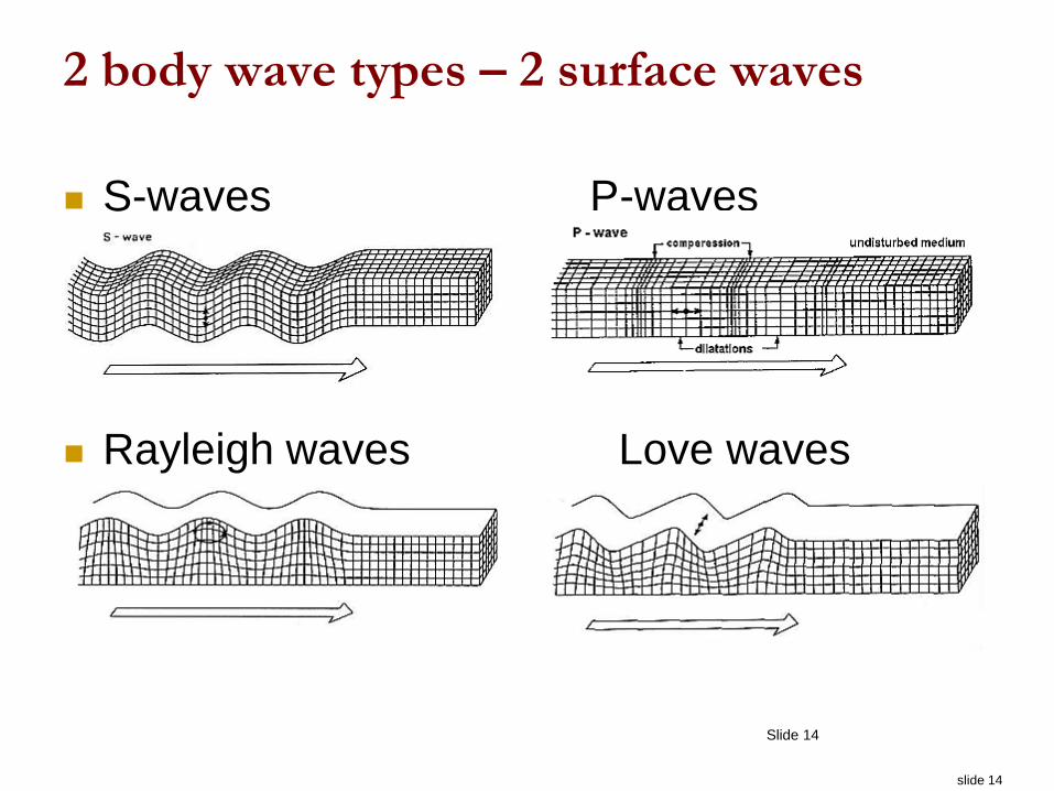
2 body wave types – 2 surface waves

S-waves P-waves

Rayleigh waves Love waves

slide 15

Slide 15

Animation of waves in a layer over a halfspace

Slower over faster (most common)

V2 > V1

V1

V2 > V1

NOTICE relation between wavefronts and signal paths (arrows)

slide 16

Seismic Applet

Direct wave

Reflected wave

slide 17

Slide 17

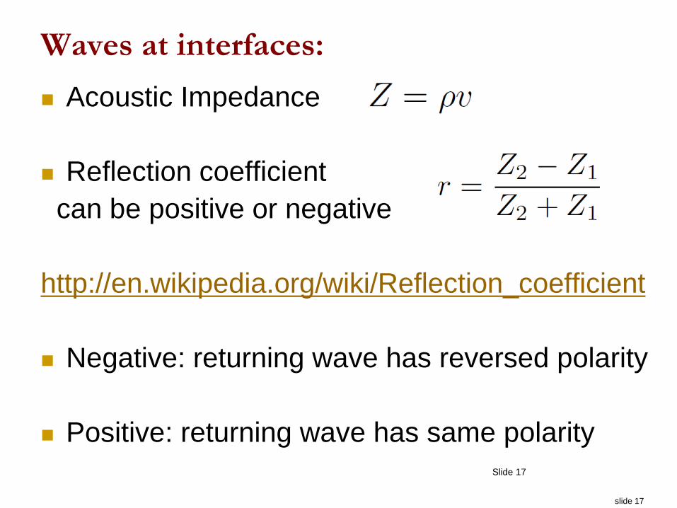
Waves at interfaces:

Acoustic Impedance

Reflection coefficient

can be positive or negative

http://en.wikipedia.org/wiki/Reflection_coefficient

Negative: returning wave has reversed polarity

Positive: returning wave has same polarity

slide 18

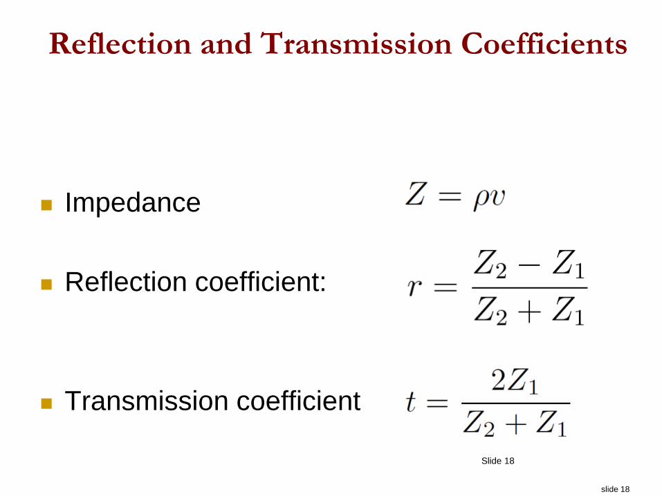
Reflection and Transmission Coefficients

Impedance

Reflection coefficient:

Transmission coefficient

Slide 18

slide 19

Seismic Refraction

slide 20

Slide 20

Energy in the ground

How many possible pathways?

How many possible pathways to one surface point?

slide 21

Seismic Applet

Direct wave

Reflected wave

Refracted wave

slide 22

Analogy for refracted waves: Swimmer

Problem

You and a friend are swimming in the ocean. Your friend

gets into problems.

What is the fastest way to reach your friend?

Slide 22

slide 23

Analogy : Swimmer Problem

You and a friend are swimming in the ocean. Your friend

gets into problems.

What is the fastest way to reach your friend?

Swim directly or take the long route by land?

Fermat’s principle or the principle of least time: the path

taken for a ray of light to travel between two points is the

path that can be traversed in the least time.

Snells’ Law can be derived from Fermat’s principle.

Slide 23

slide 24

Slide 24

Snells law

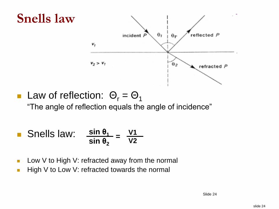
Law of reflection: Θr = Θ1

“The angle of reflection equals the angle of incidence”

Snells law:

Low V to High V: refracted away from the normal

High V to Low V: refracted towards the normal

sin θ1

sin θ2

V1

V2=

slide 25

Slide 25

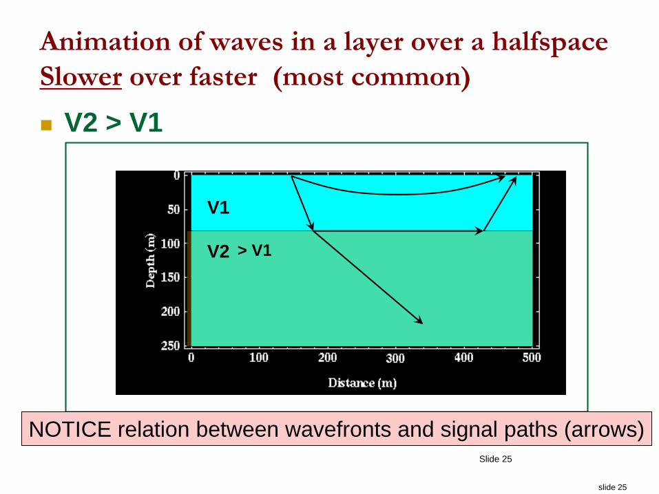
Animation of waves in a layer over a halfspace

Slower over faster (most common)

V2 > V1

V1

V2 > V1

NOTICE relation between wavefronts and signal paths (arrows)

slide 26

Slide 26

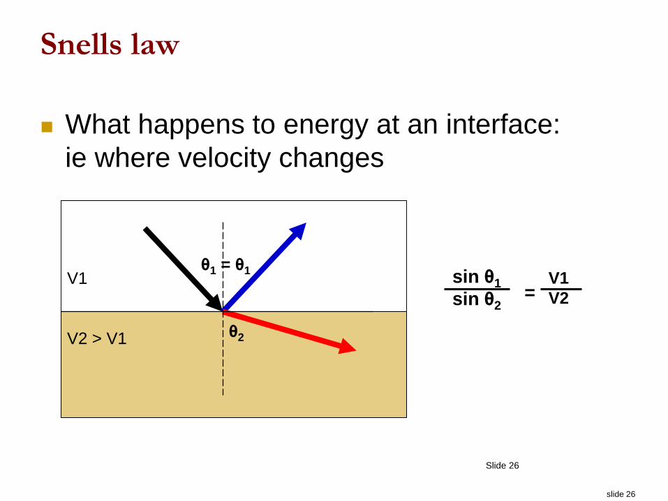
Snells law

What happens to energy at an interface:

ie where velocity changes

V1

V2 > V1

θ1 = θ1

θ2

sin θ1

sin θ2

V1

V2=

slide 27

Slide 27

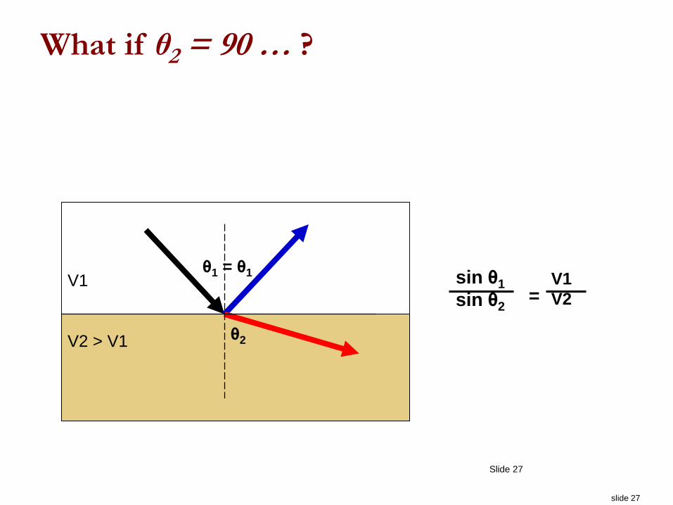
What if θ2 = 90 … ?

V1

V2 > V1

θ1 = θ1

θ2

sin θ1

sin θ2

V1

V2=

slide 28

Slide 28

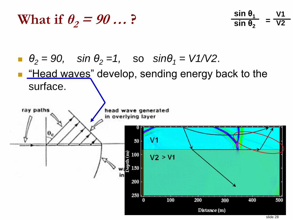
What if θ2 = 90 … ?

θ2 = 90, sin θ2 =1, so sinθ1 = V1/V2.

“Head waves” develop, sending energy back to the

surface.

sin θ1

sin θ2

V1

V2=

slide 29

Slide 29

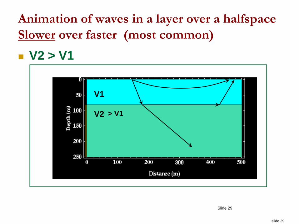
Animation of waves in a layer over a halfspace

Slower over faster (most common)

V2 > V1

V1

V2 > V1

slide 30

Slide 30

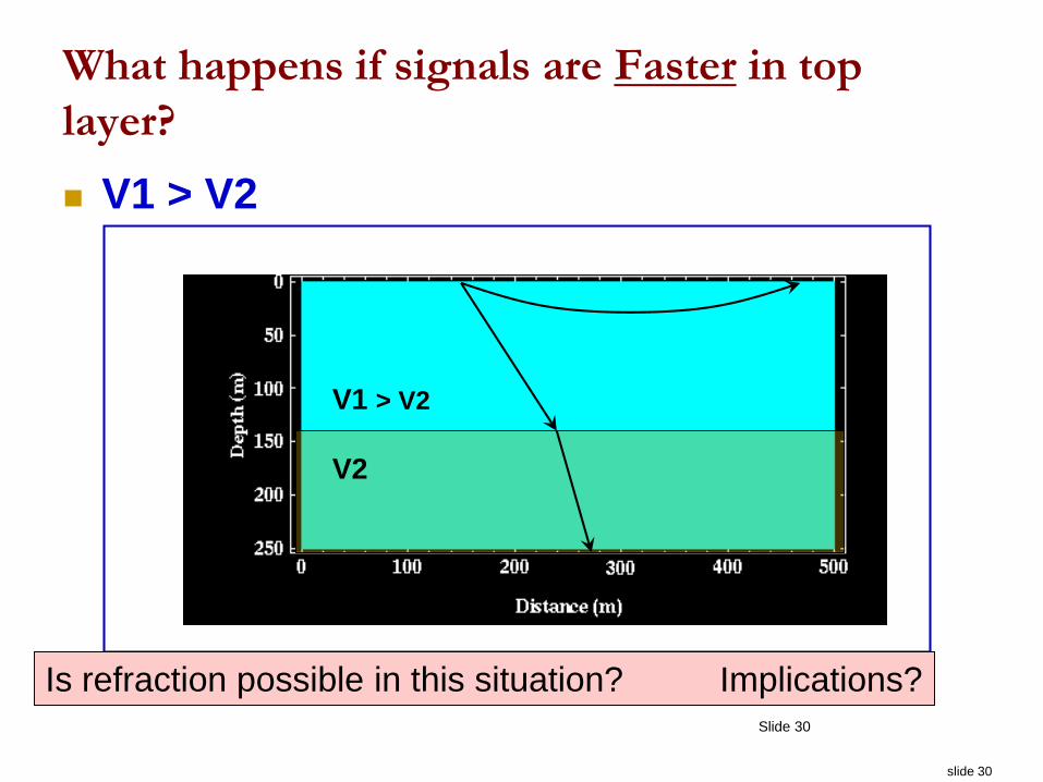
What happens if signals are Faster in top

layer?

V1 > V2

V1

V2

> V2

Is refraction possible in this situation? Implications?

slide 31

Slide 31

Java applets on the Web

http://www.phy.ntnu.edu.tw/ntnujava/index.php?topic=16

Illustration of reflection and refracted wavefronts using Fresnel-Huygens principles.

http://staff.washington.edu/aganse/raydemo/RayDemo2.med.html

Ray paths in arbitrary 1D earth. Generate the velocity model and observe first arrivals

and curved ray paths. (Visualizing bending rays in linearly increasing velocities)

http://www.iris.edu/hq/programs/education_and_outreach/visualizations

Global Earthquakes recorded by US seismometer arrays. Learn about particle motions,

wave .

slide 32

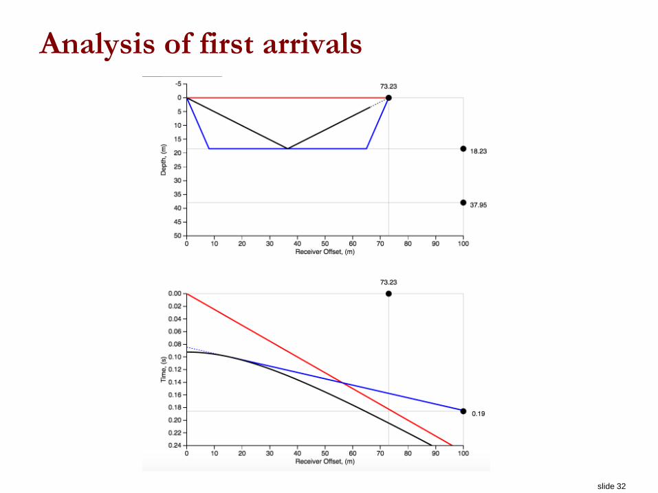
Analysis of first arrivals

slide 33

Slide 33

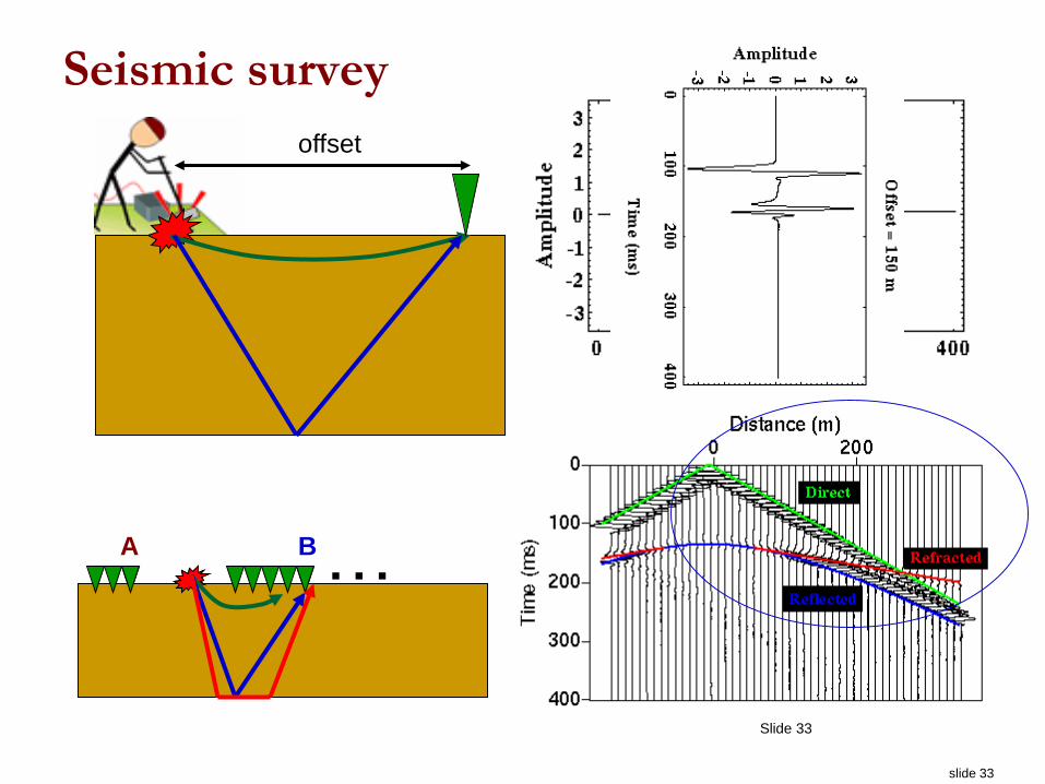
A B

A B

Seismic survey

offset

…

slide 34

Slide 34

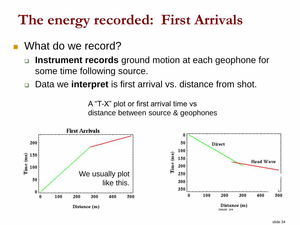
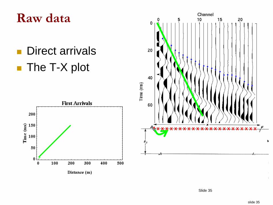
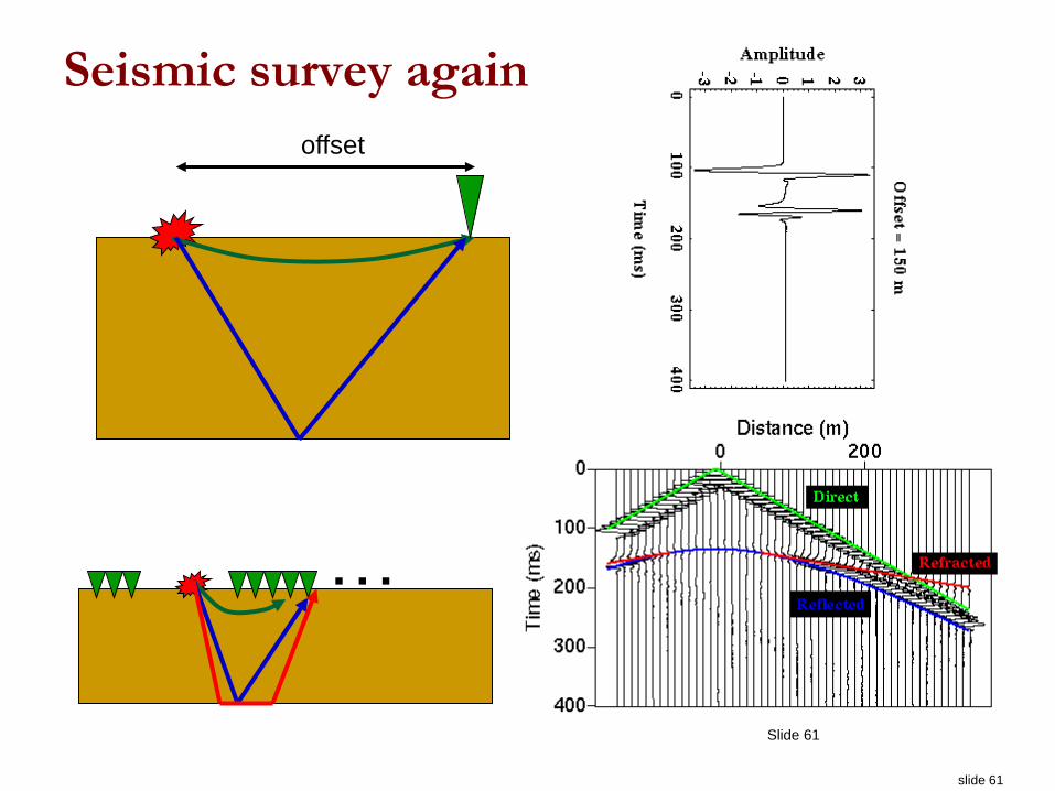
The energy recorded: First Arrivals

What do we record?

Instrument records ground motion at each geophone for

some time following source.

Data we interpret is first arrival vs. distance from shot.

A “T-X” plot or first arrival time vs

distance between source & geophones

We usually plot

like this.

slide 35

Slide 35

Raw data

Direct arrivals

The T-X plot

* x x x x x x x x x x x x x x x x x x x x x x x

slide 36

Slide 36

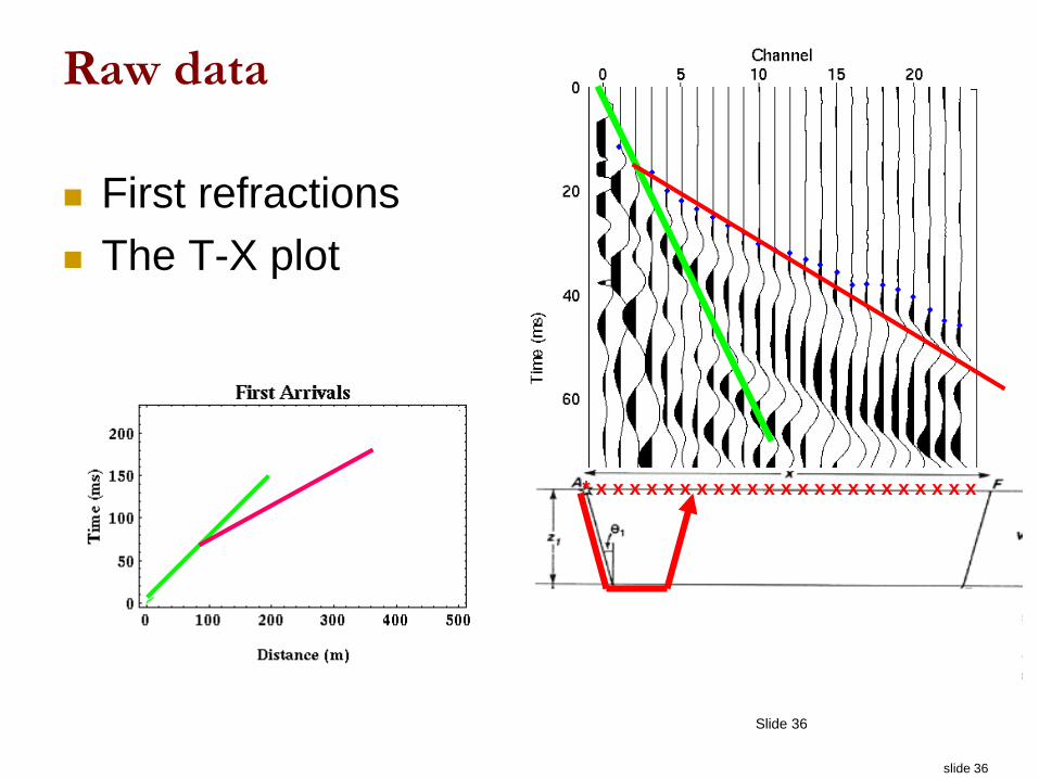
Raw data

First refractions

The T-X plot

* x x x x x x x x x x x x x x x x x x x x x x x

slide 37

Slide 37

Raw data

Second refractions

The T-X plot

* x x x x x x x x x x x x x x x x x x x x x x x

slide 38

Slide 38

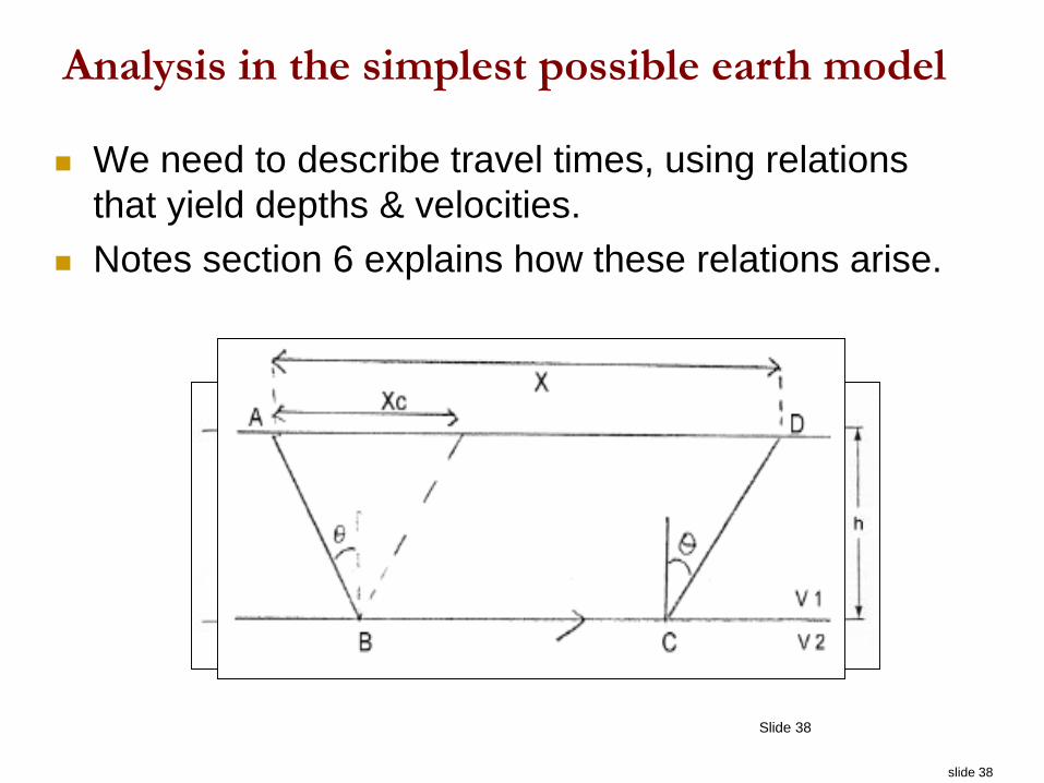
Analysis in the simplest possible earth model

We need to describe travel times, using relations

that yield depths & velocities.

Notes section 6 explains how these relations arise.

slide 39

Slide 39

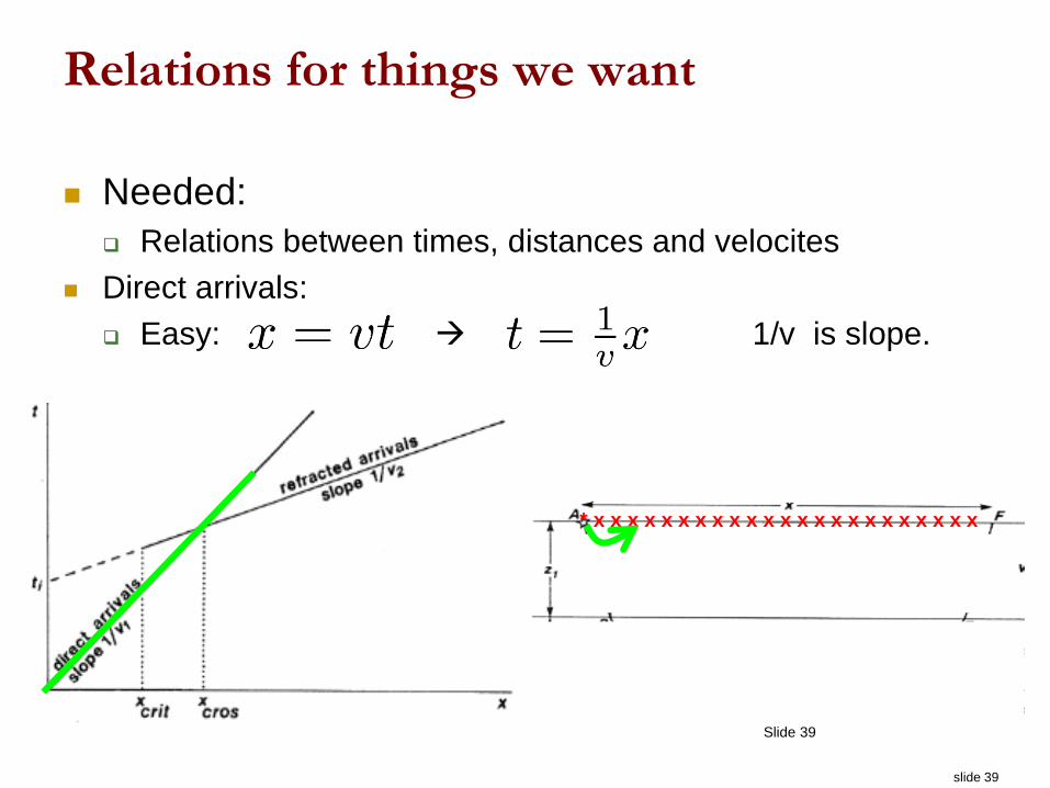
Relations for things we want

Needed:

Relations between times, distances and velocites

Direct arrivals:

Easy: 1/v is slope.

* x x x x x x x x x x x x x x x x x x x x x x x

slide 40

Slide 40

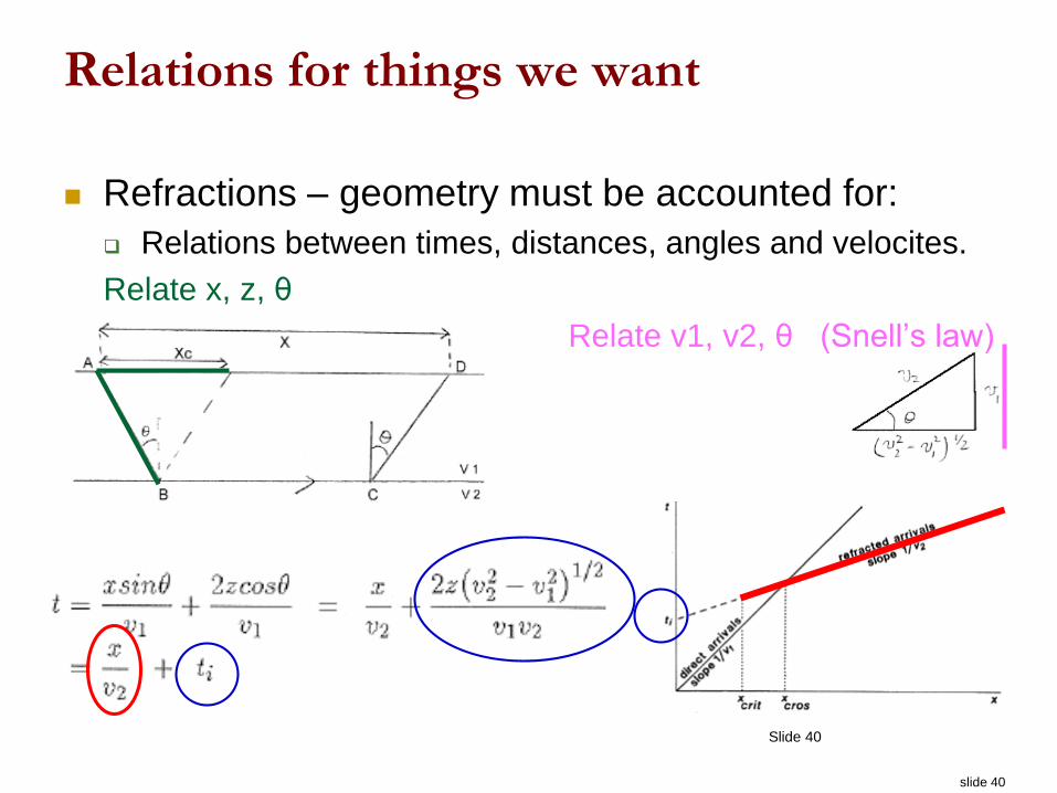
Relations for things we want

Refractions – geometry must be accounted for:

Relations between times, distances, angles and velocites.

Relate x, z, θ

Relate v1, v2, θ (Snell’s law)

slide 41

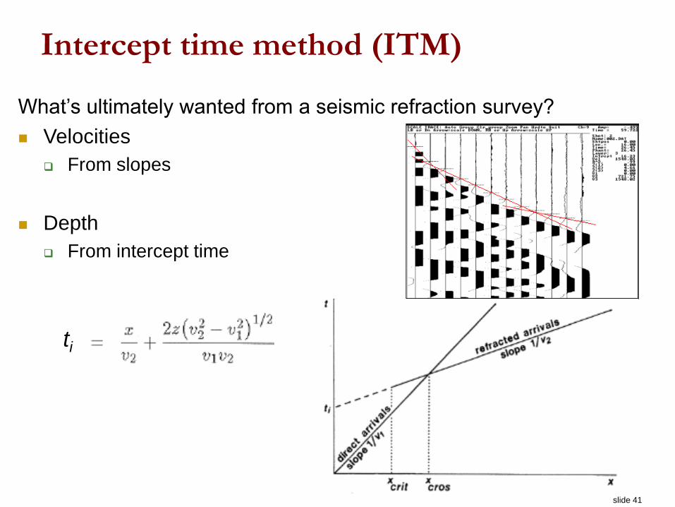
Intercept time method (ITM)

What’s ultimately wanted from a seismic refraction survey?

Velocities

From slopes

Depth

From intercept time

ti

slide 42

Slide 42

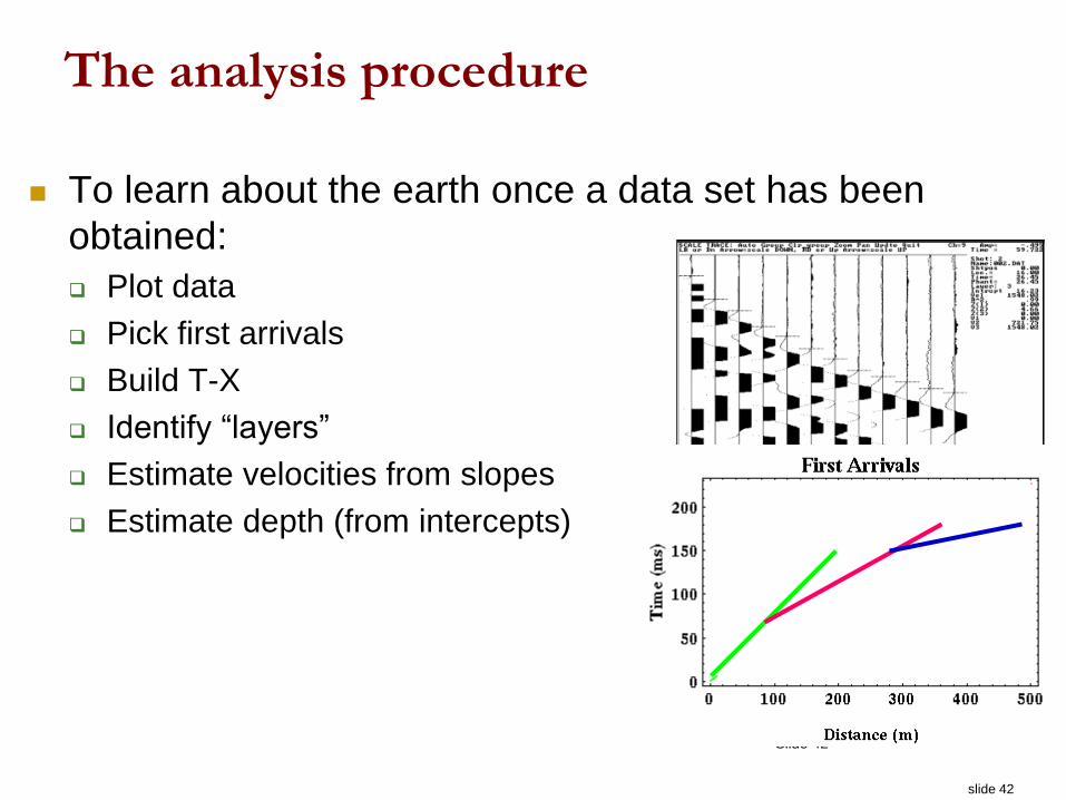
The analysis procedure

To learn about the earth once a data set has been

obtained:

Plot data

Pick first arrivals

Build T-X

Identify “layers”

Estimate velocities from slopes

Estimate depth (from intercepts)

slide 43

Slide 43

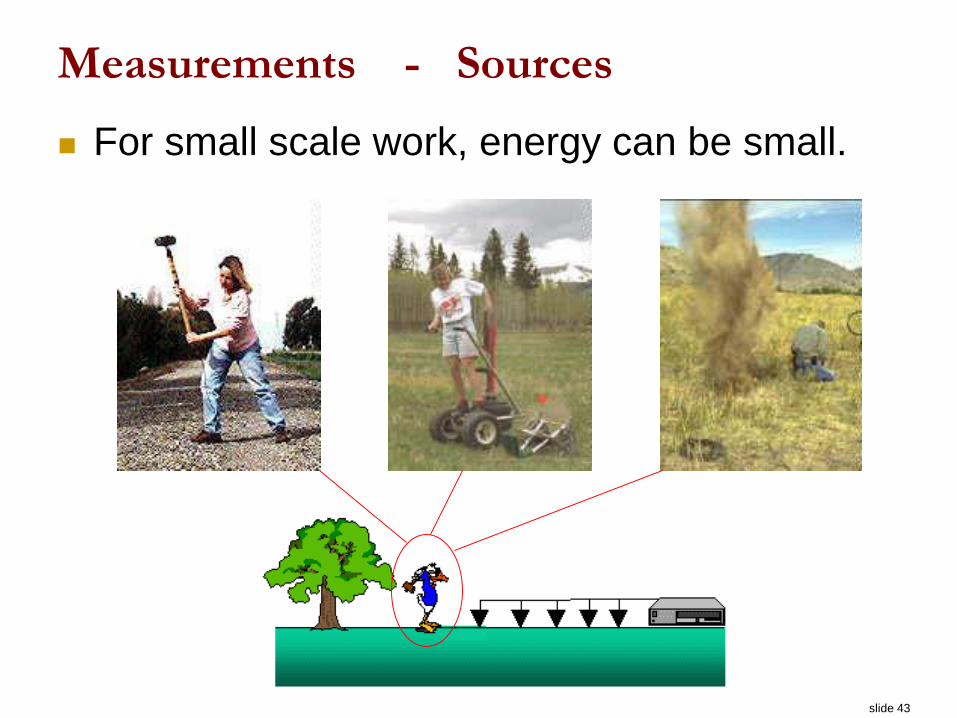
Measurements - Sources

For small scale work, energy can be small.

slide 44

Slide 44

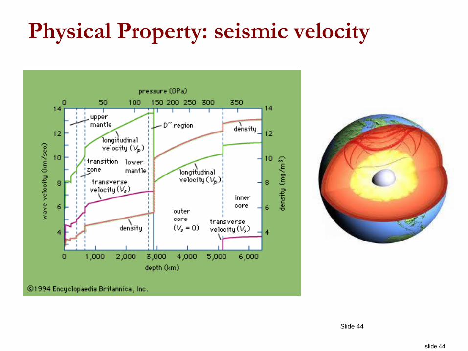
Physical Property: seismic velocity

slide 45

Seismic Survey

Sources: anything that causes earth particles

to move:

Natural: (earthquakes)

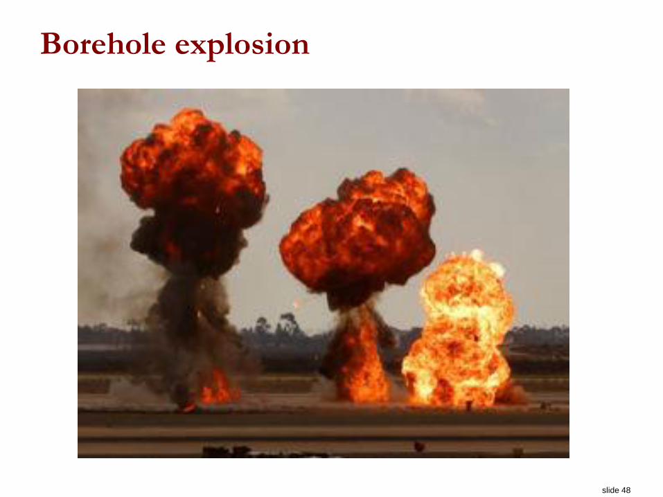
Man-made: explosives, “hammers”, shock waves

Receivers: measure

Displacement

Velocity

Acceleration

Slide 45

slide 46

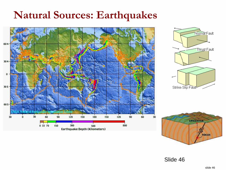
Natural Sources: Earthquakes

Slide 46

slide 47

EOSC 350 2010

Slide 47

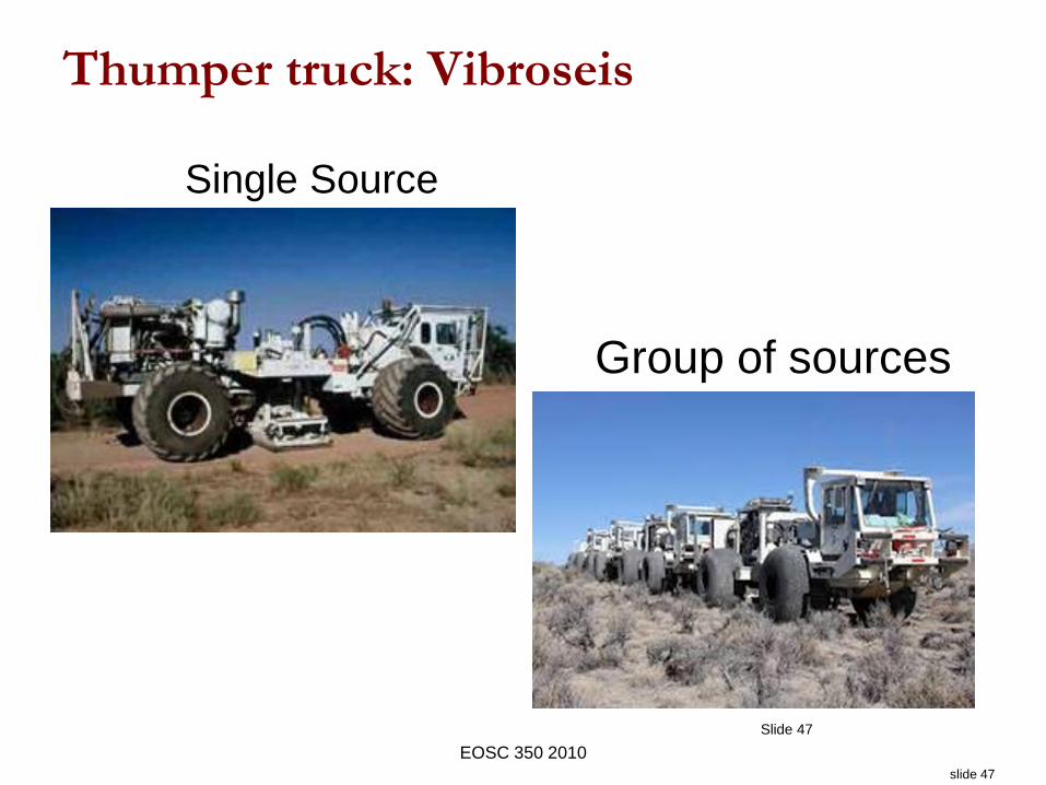
Thumper truck: Vibroseis

Group of sources

Single Source

slide 48

Borehole explosion

slide 49

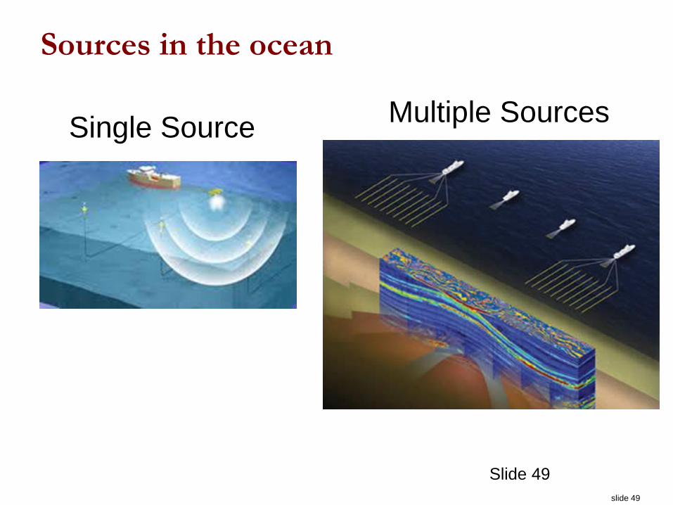
Sources in the ocean

Slide 49

Single SourceMultiple Sources

slide 50

Slide 50

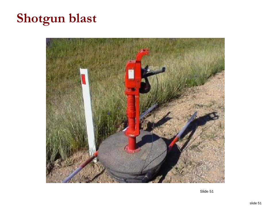
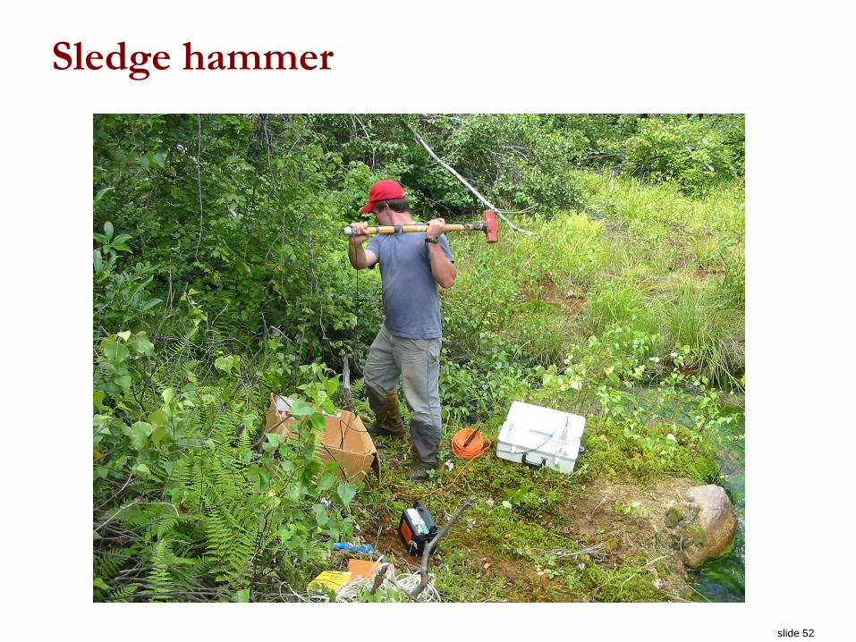
Measurements - Sources

For small scale work, energy can be small.

slide 51

Slide 51

Shotgun blast

slide 52

Slide 52

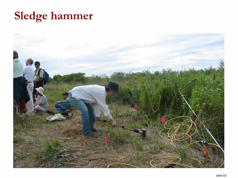
Sledge hammer

slide 53

Slide 53

Sledge hammer

slide 54

Slide 54

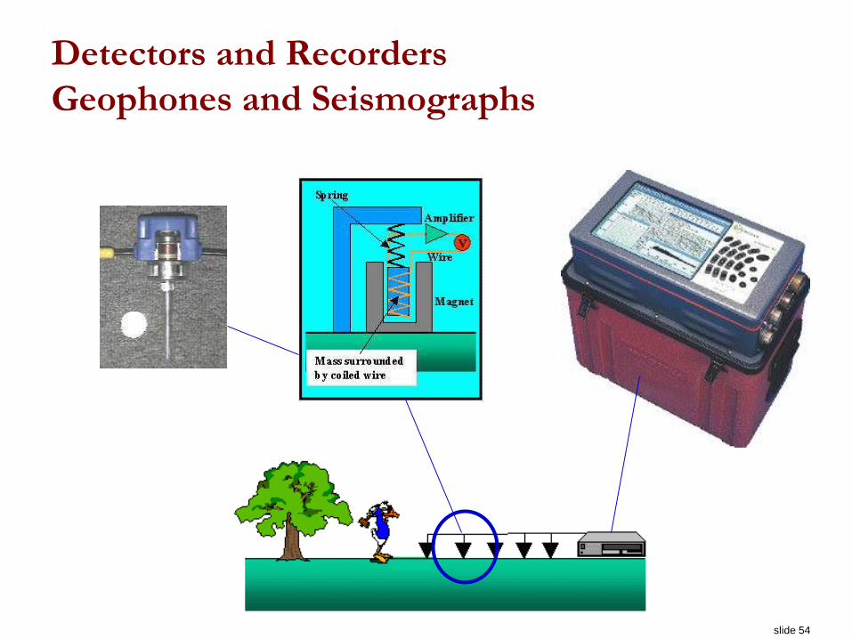
Detectors and Recorders

Geophones and Seismographs

slide 55

Slide 55

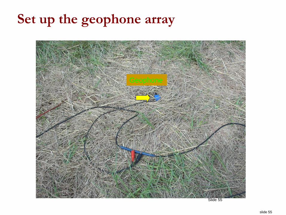
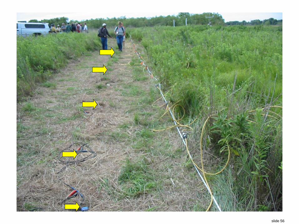
Set up the geophone array

Geophone

slide 56

Slide 56

slide 57

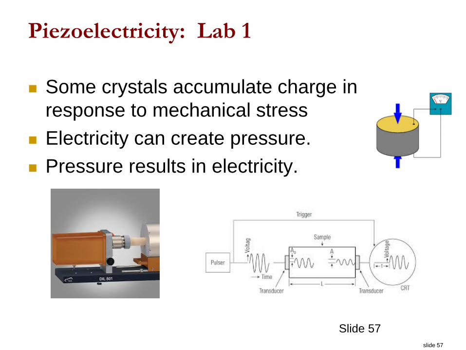
Piezoelectricity: Lab 1

Some crystals accumulate charge in

response to mechanical stress

Electricity can create pressure.

Pressure results in electricity.

Slide 57

slide 58

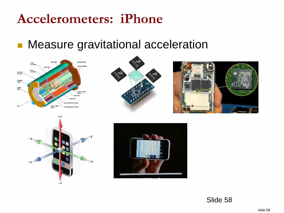
Accelerometers: iPhone

Measure gravitational acceleration

Slide 58

slide 59

iPhone examples

iPhone app: iSeismometer

Slide 59

slide 60

Slide 60

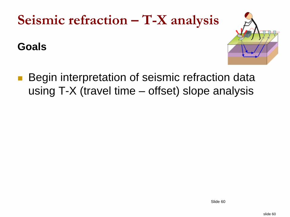
Seismic refraction – T-X analysis

Goals

Begin interpretation of seismic refraction data

using T-X (travel time – offset) slope analysis

slide 61

Slide 61

Seismic survey again

offset

…

slide 62

Slide 62

Readings

Seismic refraction: GPG 3.e.7 - 3.e8

slide 63

Slide 63

Other topics

Low Velocity Zones

Refraction for multiple layers.

Dipping Layers

More complicated interfaces and approaches. Plus-Minus method Generalized Reciprocal Method Ray Tracing

slide 64

Low Velocity Zone

Snell’s law for decreasing velocity

http://staff.washington.edu/aganse/raydemo/RayDemo2.med.html

Ray tracing for non-layered velocity models (Illustration of Snell’s law)

slide 65

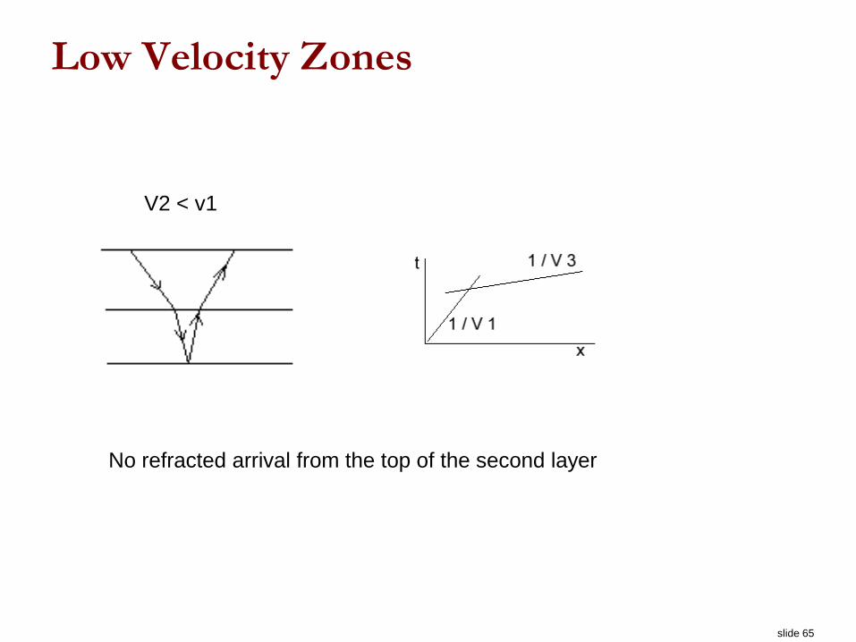
Low Velocity Zones

V2 < v1

No refracted arrival from the top of the second layer

slide 66

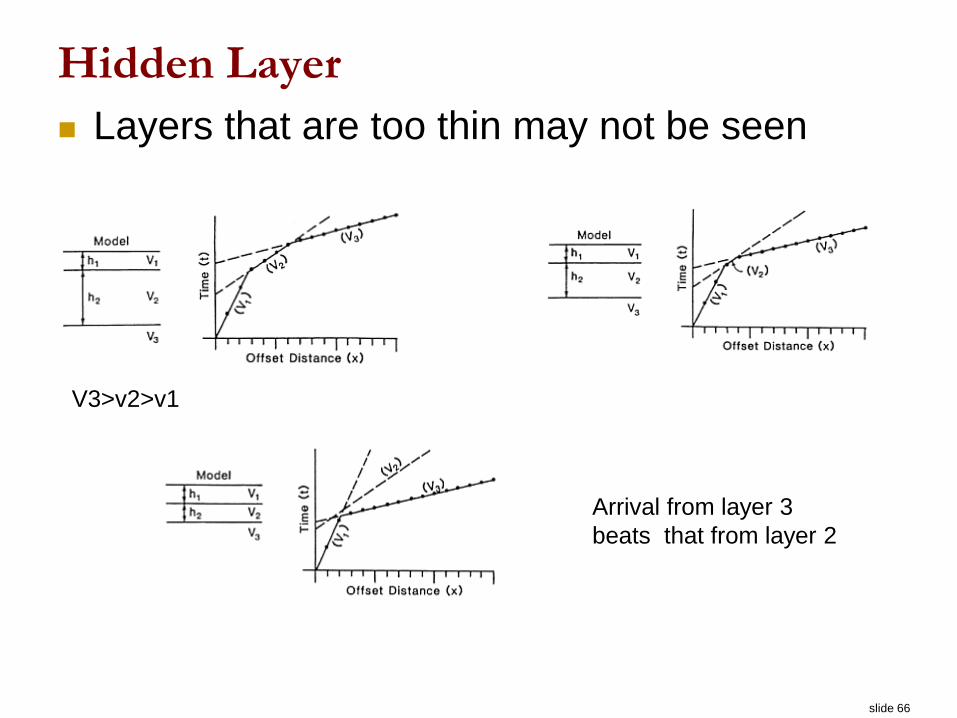
Hidden Layer

Layers that are too thin may not be seen

Arrival from layer 3

beats that from layer 2

V3>v2>v1

slide 67

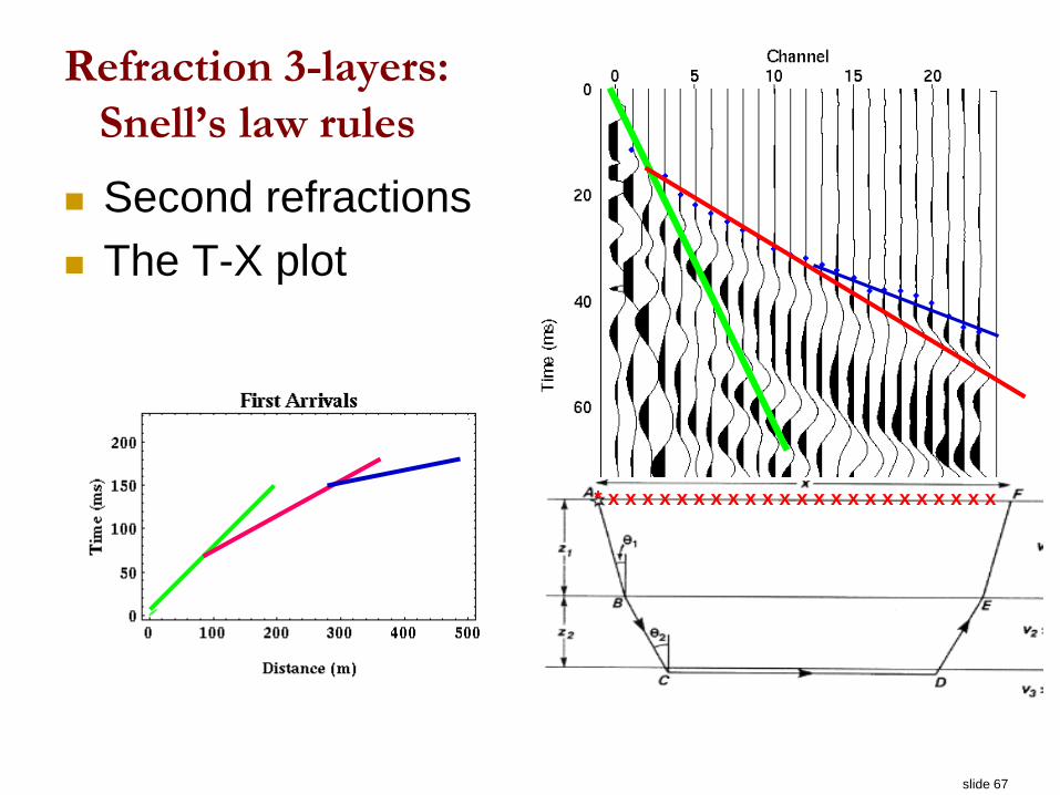
Refraction 3-layers:

Snell’s law rules

Second refractions

The T-X plot

* x x x x x x x x x x x x x x x x x x x x x x x

slide 68

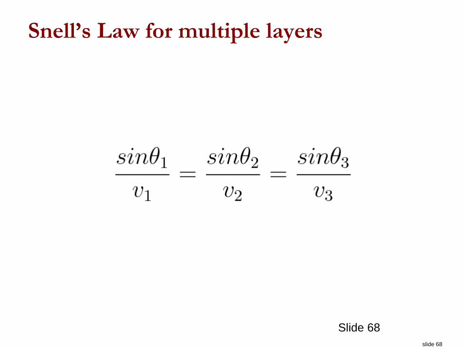
Snell’s Law for multiple layers

Slide 68

slide 69

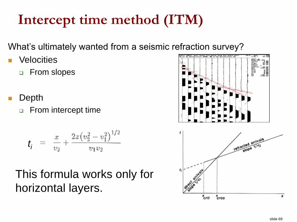
Intercept time method (ITM)

What’s ultimately wanted from a seismic refraction survey?

Velocities

From slopes

Depth

From intercept time

ti

This formula works only for

horizontal layers.

slide 70

EOSC 350 ‘06 Slide 70

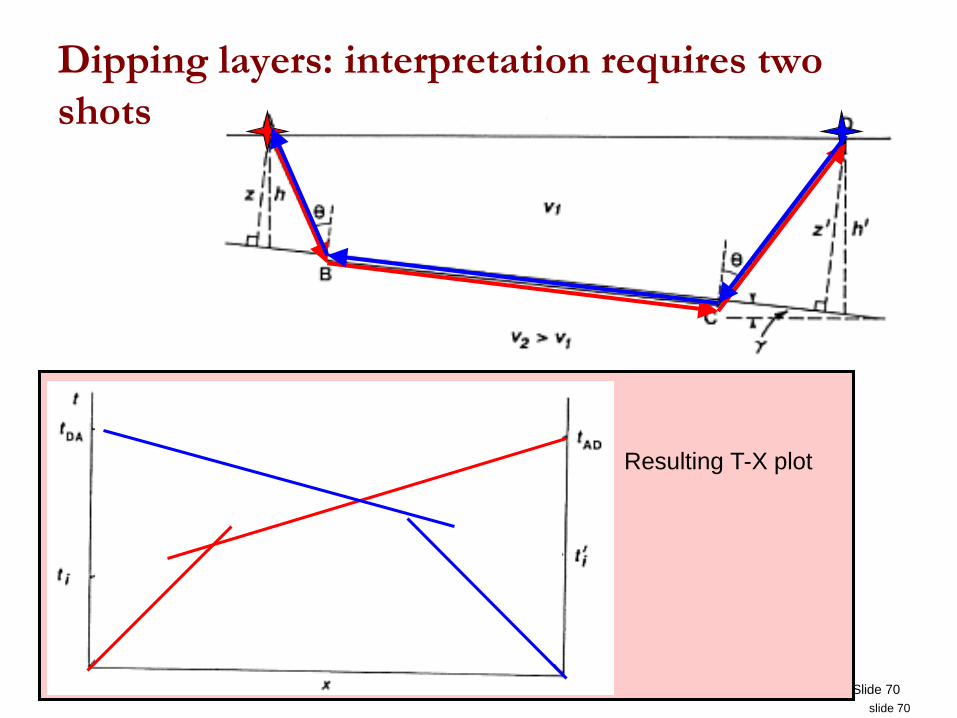
Dipping layers: interpretation requires two

shots

Resulting T-X plot

slide 71

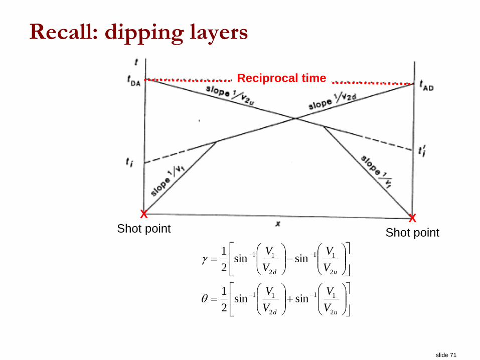
Recall: dipping layers

ud

ud

V

V

V

V

V

V

V

V

2

11

2

11

2

11

2

11

sinsin2

1

sinsin2

1

X

Shot pointX

Shot point

Reciprocal time

slide 72

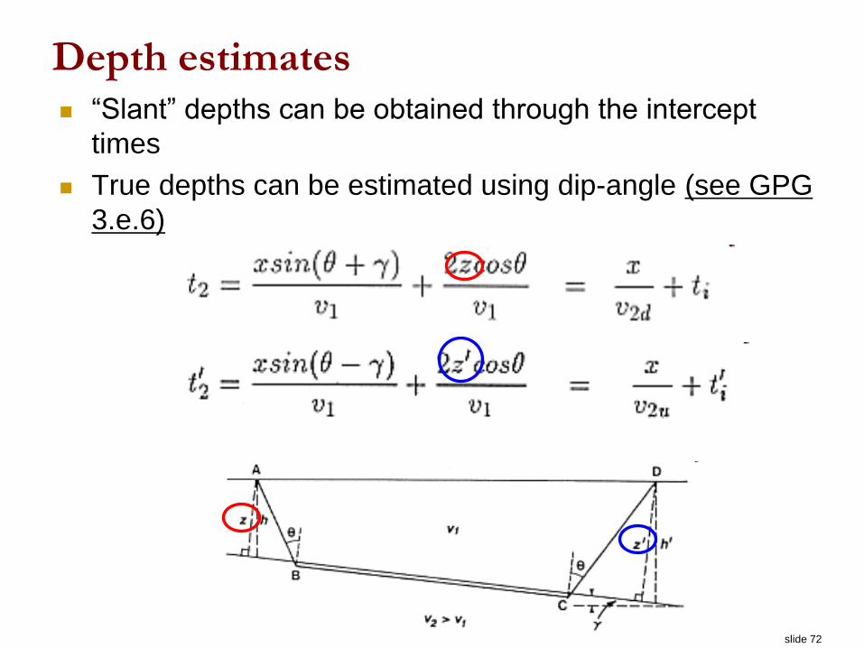
Depth estimates “Slant” depths can be obtained through the intercept

times

True depths can be estimated using dip-angle (see GPG

3.e.6)

slide 73

Irregular Layers

What happens when the boundary can no

longer be approximated with a plane?

Plus-Minus Methods

GRM (Generalized Reciprocal Methods)

Ray tracing

Other sophisticated procedures.

slide 74

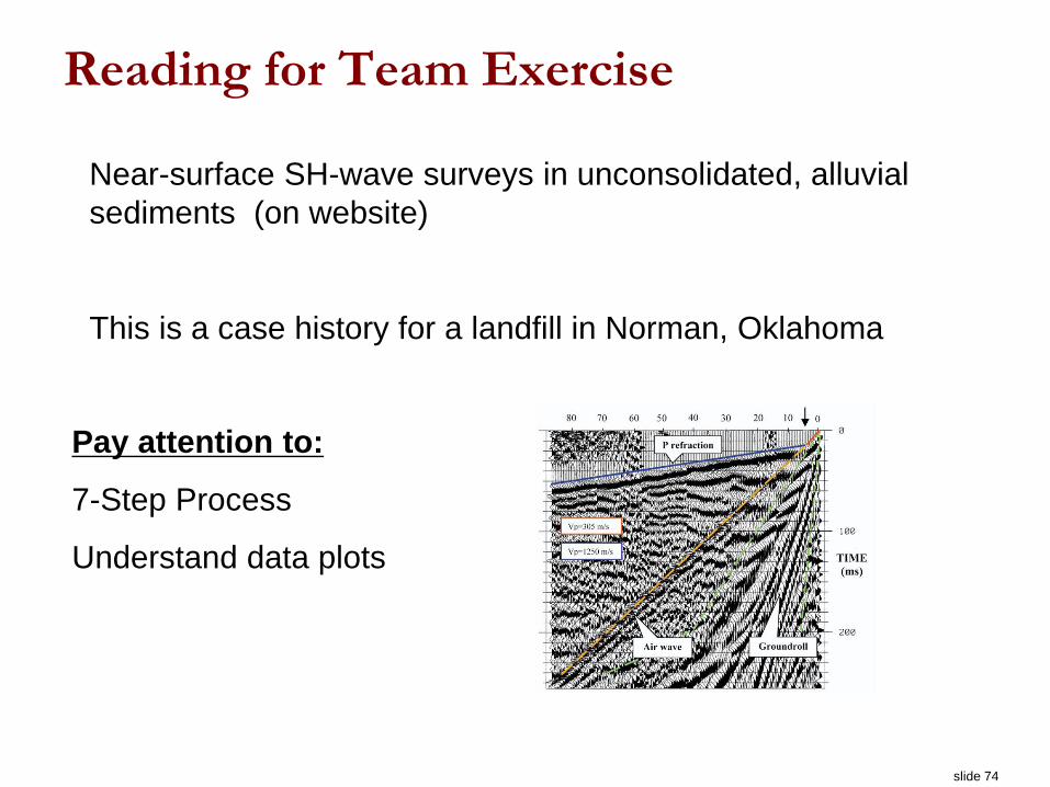
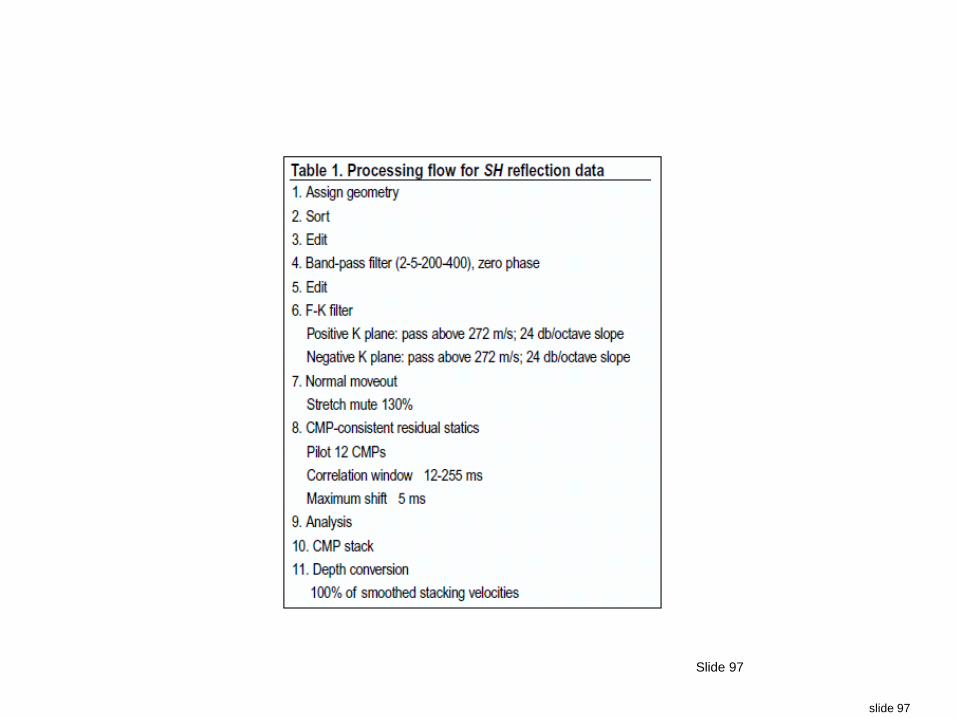
Reading for Team Exercise

Near-surface SH-wave surveys in unconsolidated, alluvial

sediments (on website)

This is a case history for a landfill in Norman, Oklahoma

Pay attention to:

7-Step Process

Understand data plots

slide 75

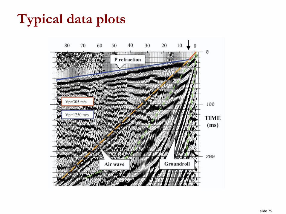
Typical data plots

slide 76

Reflection Seismology

Slide 76

slide 77

EOSC 350 2010 Slide 77

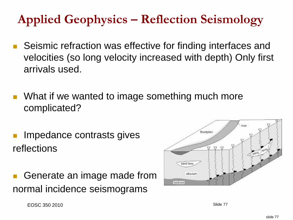
Applied Geophysics – Reflection Seismology

Seismic refraction was effective for finding interfaces and

velocities (so long velocity increased with depth) Only first

arrivals used.

What if we wanted to image something much more

complicated?

Impedance contrasts gives

reflections

Generate an image made from

normal incidence seismograms

slide 78

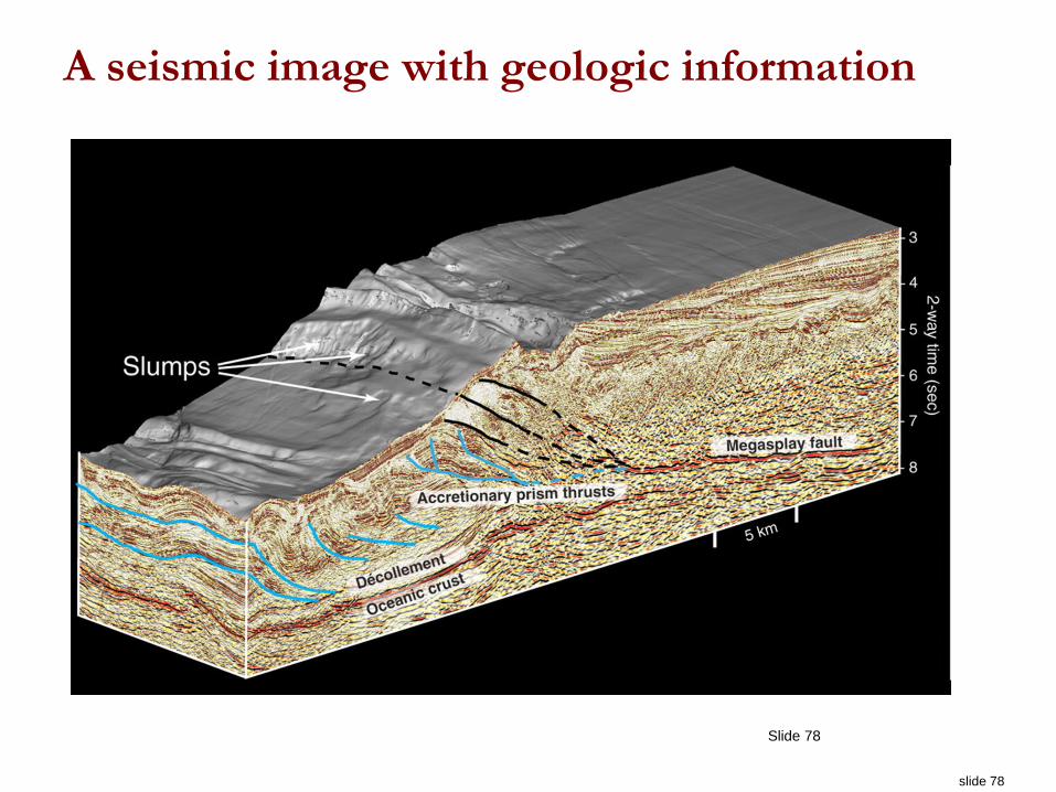
A seismic image with geologic information

Slide 78

slide 79

Slide 79

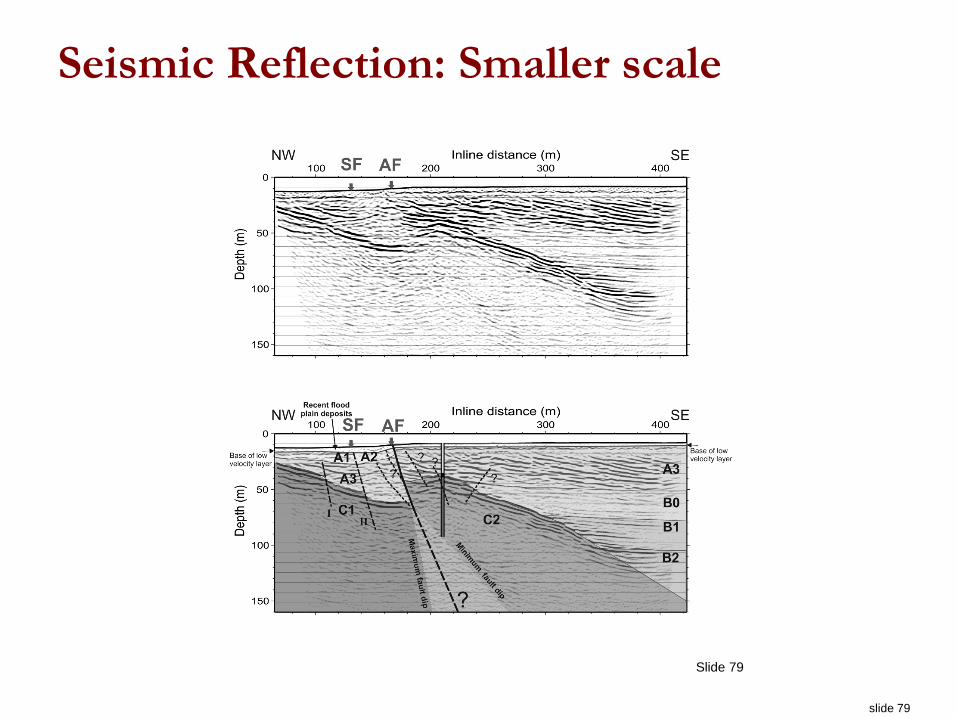
Seismic Reflection: Smaller scale

slide 80

Main uses for reflection seismology

Hydrocarbon exploration!!!

General earth structure:

Whole earth

Continental scale (lithoprobe)

Regional scales

Local structure: geotechnical and

environmental work

Slide 80

slide 81

Slide 81

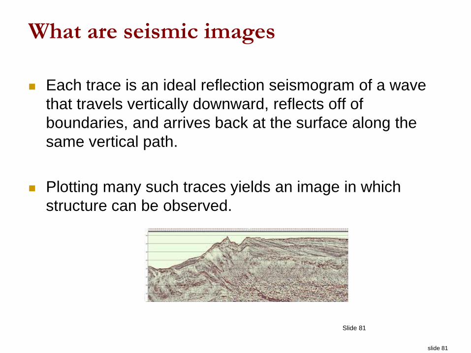
What are seismic images

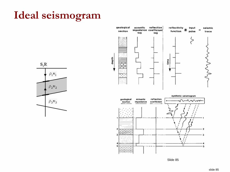
Each trace is an ideal reflection seismogram of a wave

that travels vertically downward, reflects off of

boundaries, and arrives back at the surface along the

same vertical path.

Plotting many such traces yields an image in which

structure can be observed.

slide 82

Slide 82

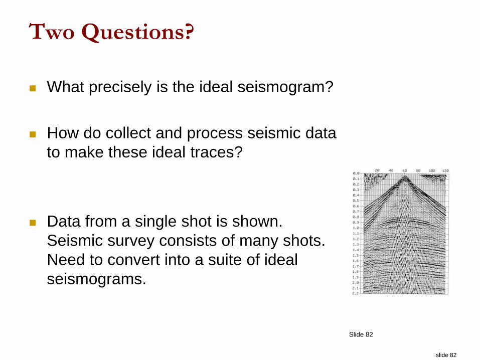
Two Questions?

What precisely is the ideal seismogram?

How do collect and process seismic data

to make these ideal traces?

Data from a single shot is shown.

Seismic survey consists of many shots.

Need to convert into a suite of ideal

seismograms.

slide 83

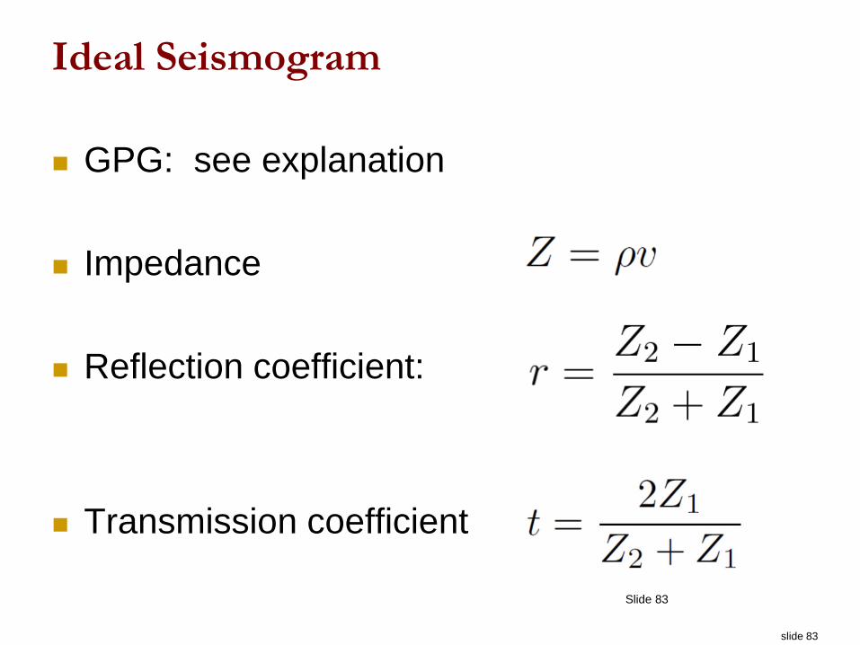
Ideal Seismogram

GPG: see explanation

Impedance

Reflection coefficient:

Transmission coefficient

Slide 83

slide 84

Slide 84

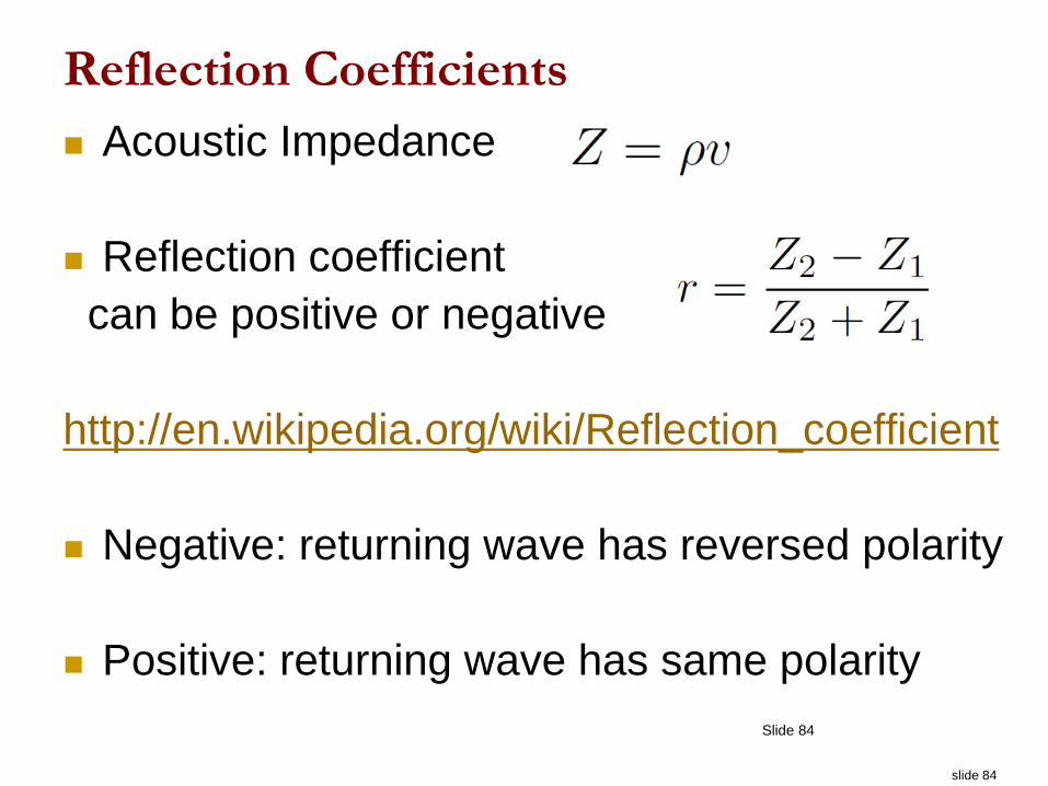
Reflection Coefficients

Acoustic Impedance

Reflection coefficient

can be positive or negative

http://en.wikipedia.org/wiki/Reflection_coefficient

Negative: returning wave has reversed polarity

Positive: returning wave has same polarity

slide 85

Ideal seismogram

Slide 85

slide 86

Slide 86

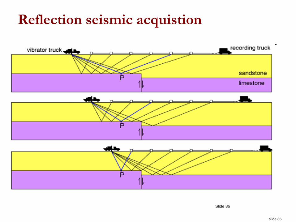
Reflection seismic acquistion

slide 87

Slide 87

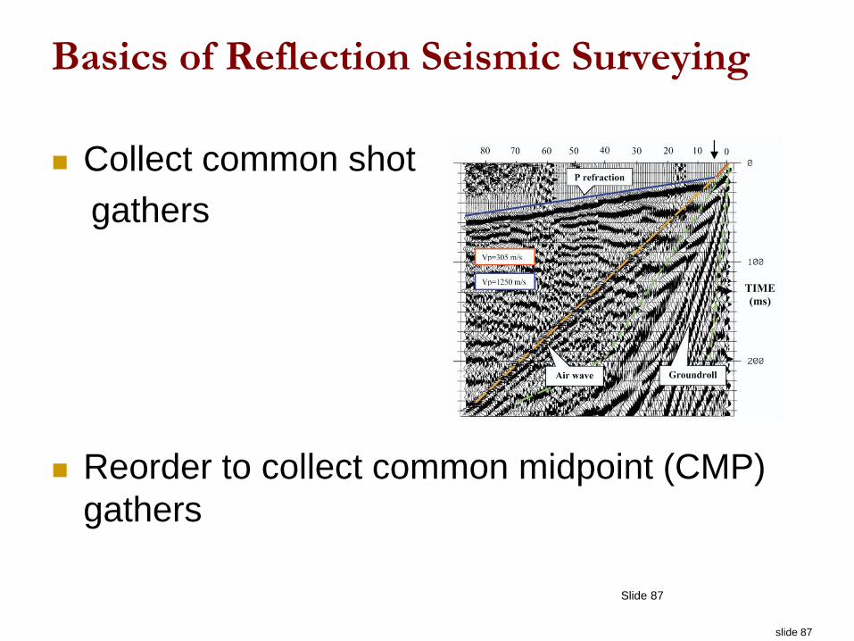
Basics of Reflection Seismic Surveying

Collect common shot

gathers

Reorder to collect common midpoint (CMP)

gathers

slide 88

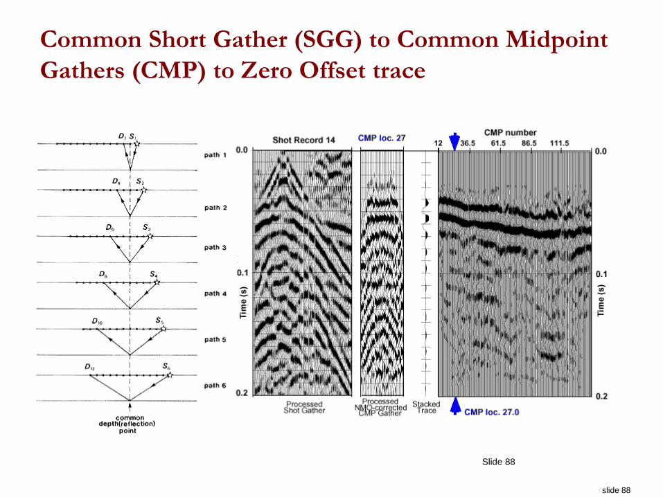
Common Short Gather (SGG) to Common Midpoint

Gathers (CMP) to Zero Offset trace

Slide 88

slide 89

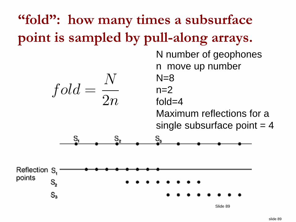
“fold”: how many times a subsurface

point is sampled by pull-along arrays.

Slide 89

N number of geophones

n move up number

N=8

n=2

fold=4

Maximum reflections for a

single subsurface point = 4

slide 90

Slide 90

Some Common Shot Gathers

slide 91

Slide 91

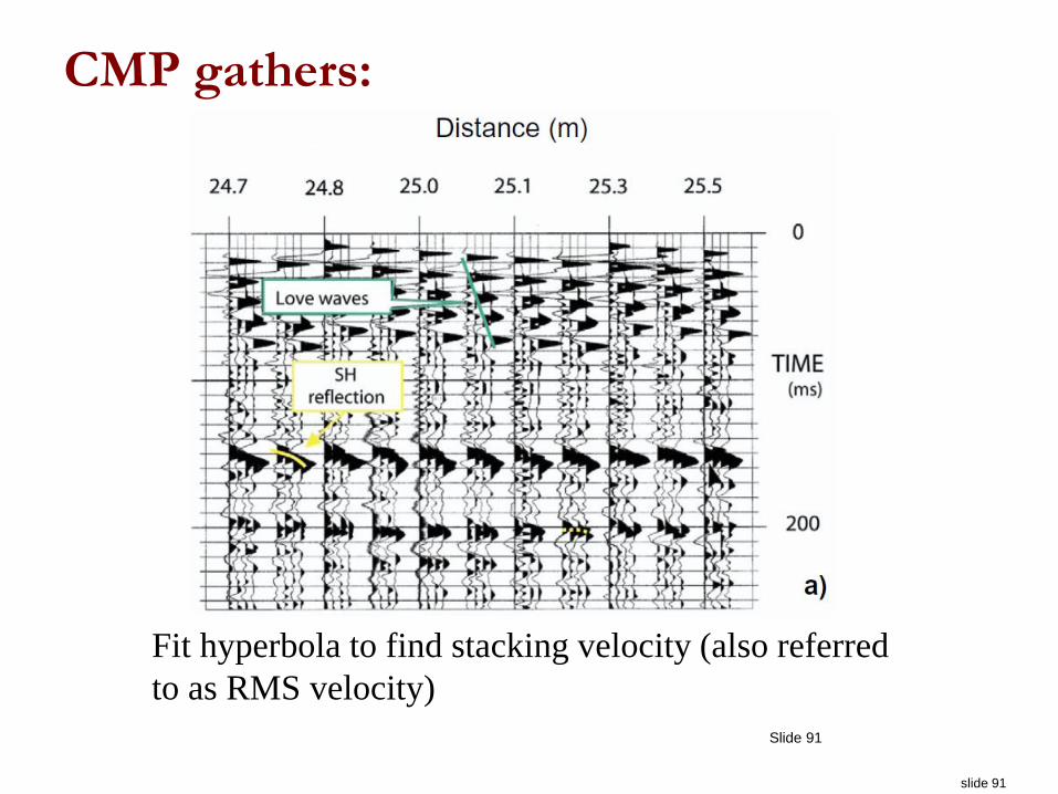
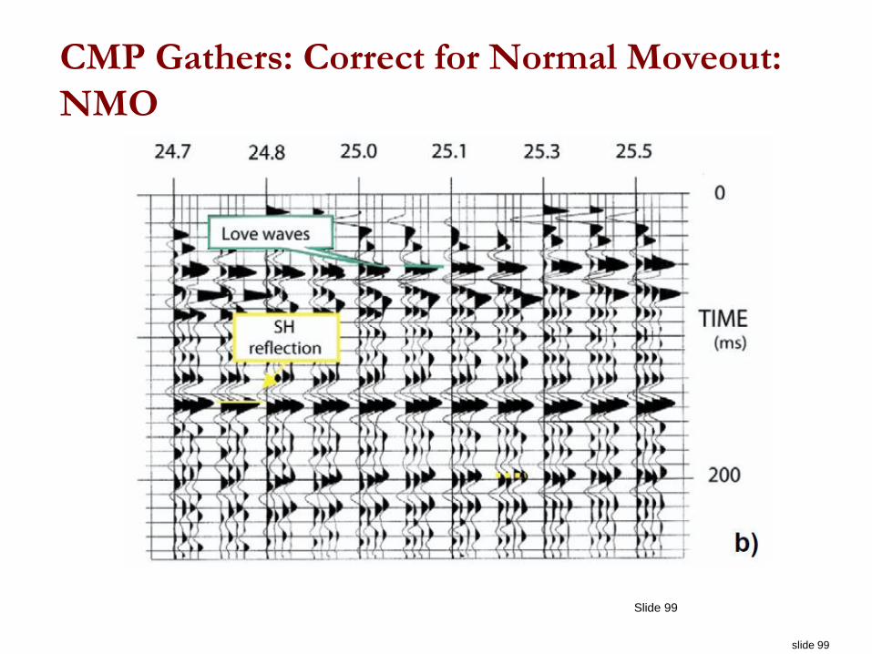
CMP gathers:

Fit hyperbola to find stacking velocity (also referred

to as RMS velocity)

slide 92

Slide 92

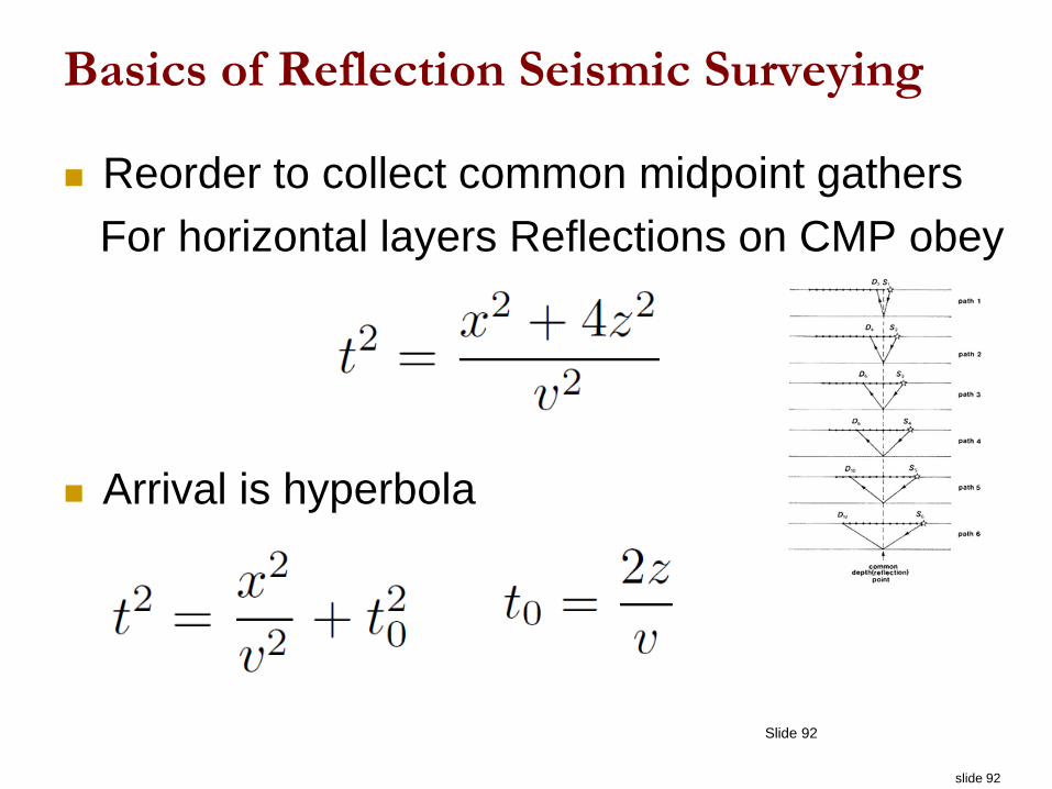
Basics of Reflection Seismic Surveying

Reorder to collect common midpoint gathers

For horizontal layers Reflections on CMP obey

Arrival is hyperbola

slide 93

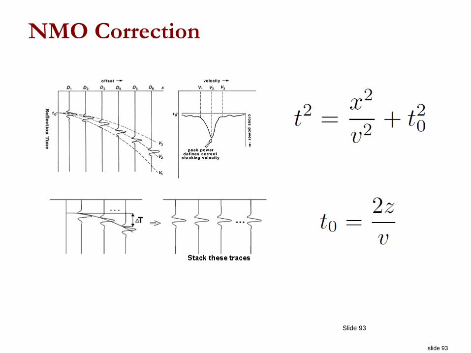
NMO Correction

Slide 93

slide 94

Slide 94

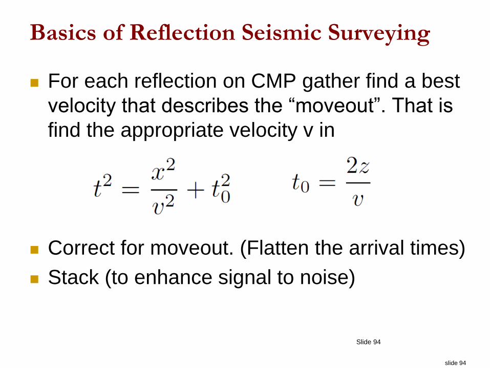
Basics of Reflection Seismic Surveying

For each reflection on CMP gather find a best

velocity that describes the “moveout”. That is

find the appropriate velocity v in

Correct for moveout. (Flatten the arrival times)

Stack (to enhance signal to noise)

slide 95

Slide 95

Basics of Reflection Seismic Surveying

Stack (to enhance signal to noise). The number of

traces in the stack is called the “fold”

Result is one seismic trace for each CMP gather.

Put all traces together. Interpret as vertical wave

propagating down and reflecting upwards

Interpret geologically. (Polarity is important)

slide 96

Slide 96

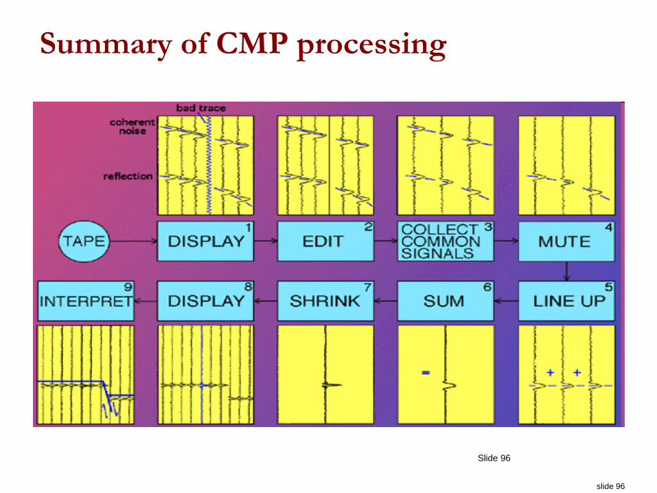
Summary of CMP processing

slide 97

Slide 97

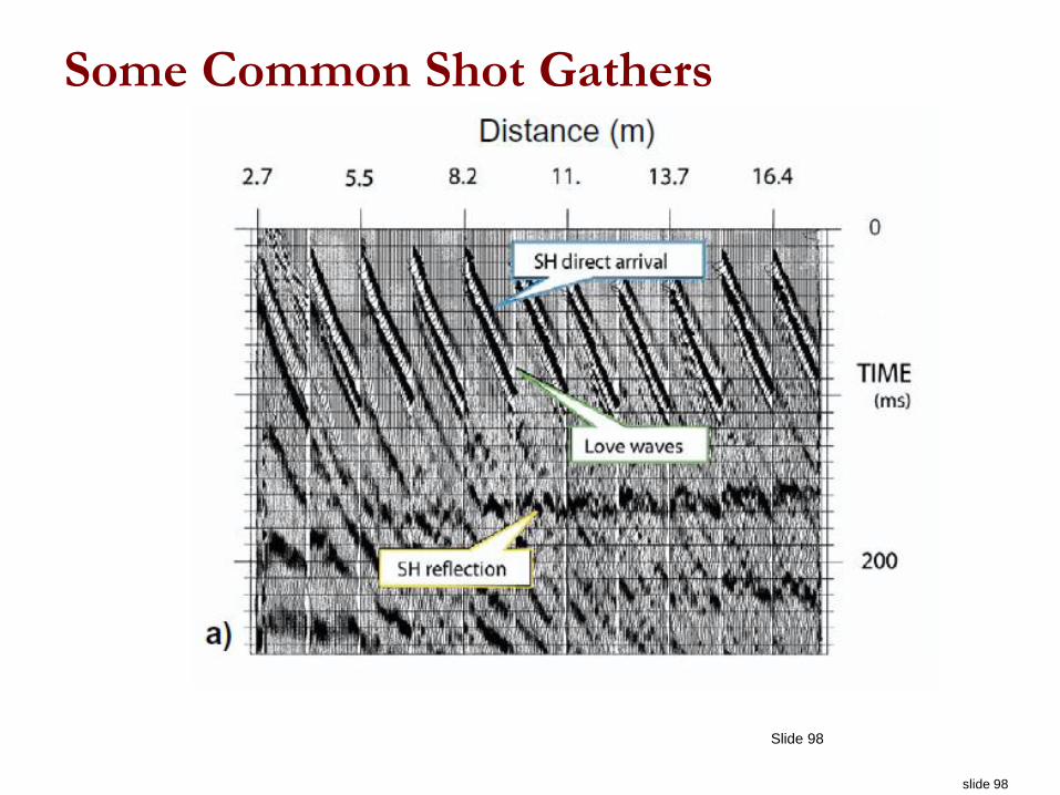
slide 98

Slide 98

Some Common Shot Gathers

slide 99

Slide 99

CMP Gathers: Correct for Normal Moveout:

NMO

slide 100

Slide 100

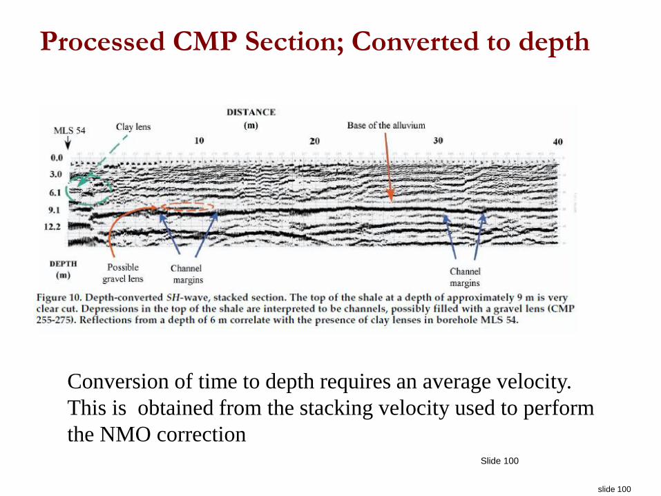
Processed CMP Section; Converted to depth

Conversion of time to depth requires an average velocity.

This is obtained from the stacking velocity used to perform

the NMO correction

slide 101

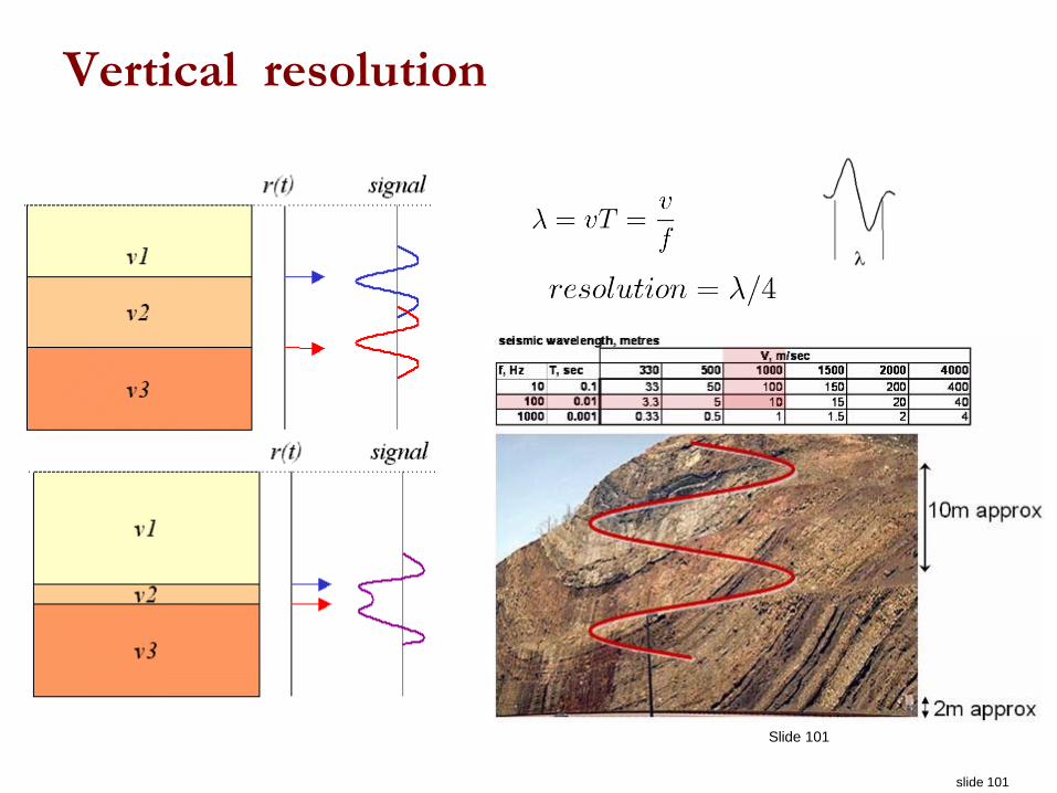
Vertical resolution

Slide 101

slide 102

Geotechnical applications for reflection

seismology

slide 104

MASW

Multichannel Analysis of Surface Waves

Slide 104

slide 105

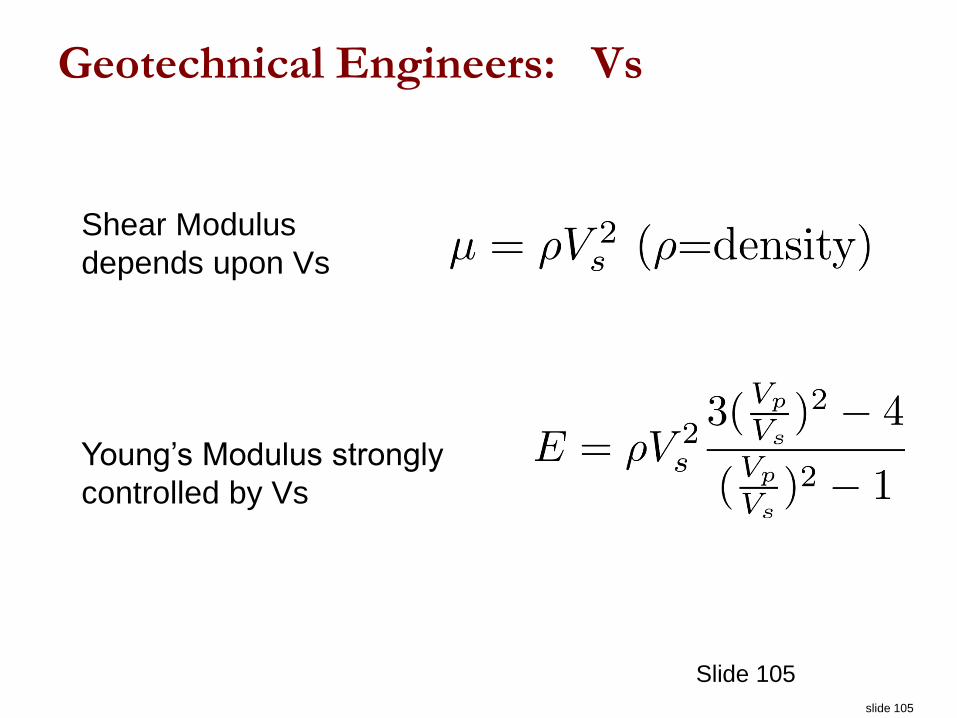
Geotechnical Engineers: Vs

Slide 105

Shear Modulus

depends upon Vs

Young’s Modulus strongly

controlled by Vs

slide 106

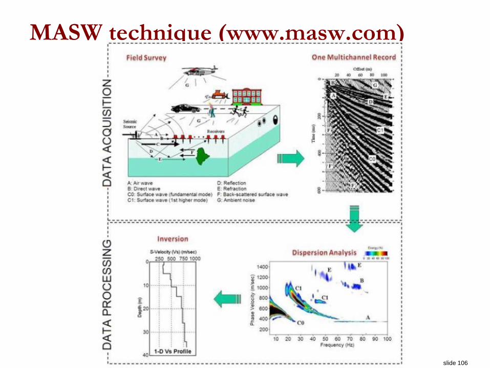
MASW technique (www.masw.com)

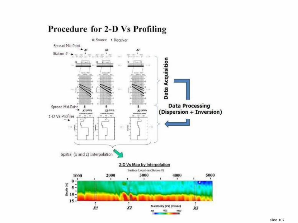
slide 107

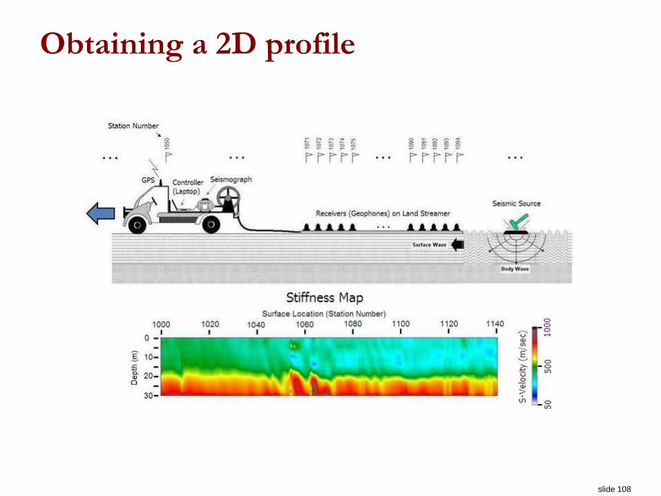
slide 108

Obtaining a 2D profile

slide 109

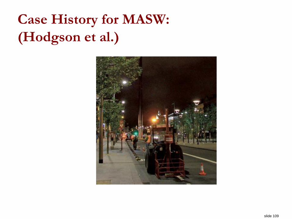
Case History for MASW:

(Hodgson et al.)

slide 110

Dublin: Case History for MASW

Setup: Dublin underlain by Dublin boulder clay (DBC).

Hard lodgement till with high stiffness and low

permeability. Large cobbles and boulders above DBC.

Properties: elastic parameters, stiffness is related to

shear velocity

Survey: Seismic. MASW

Data Acquisition: Roll-along survey. Land streamer 24

plated-coupled 4.5Hz geophones. Tractor-mounted

weight drop with shots every 6m.

slide 111

Dublin: MASW

Analysis: Dispersion curve analysis of surface waves.

Invert to obtain Vs. Generate a 2D profile.

Interpretation: Low Vs (200-700 m/s) associated with

glacial till (0-10m thickness. High velocity material

(Vs>900 m/s) at depth

slide 112

MASW

Dublin

slide 113

Dublin: MASW

Interpretation: Low Vs (200-700 m/s) associated with

glacial till (0-10m thickness. High velocity material

(Vs>900 m/s) at depth

Synthesize: Borehole verified the high velocity material

as limestone bedrock. The depth is variable.

slide 114

Next week

Monday: Thanksgiving No Lecture/Lab

Wednesday: Guest: Mike Maxwell Golder Assoc

Friday: TBL (Seismology)

slide 115

End Seismology

Slide 115

slide 116

slide 117