1

Shear Wave Profiles of Roadway Substructures from MASW and Waveform Tomography

Khiem T. Tran1, Justin Sperry2, Michael McVay3, Scott J. Wasman4, and David Horhota5

ABSTRACT:

Assessment of roadway subsidence due to embedded low-velocity anomalies is critical to the health and safety of the traveling public. Surface-based seismic techniques are often used to assess roadways because of data acquisition convenience and large depths of characterization. To mitigate the negative time impact of closing a traffic lane under traditional seismic testing, a new land-streamer test system is presented. The main advantage of using the new land-streamer system is the elimination of the need of coupling the geophones to the roadway, the use of only one source at the end of geophone array, and the movement of the whole test system along the roadway quickly. For demonstration, experimental data was collected on asphalt pavement overlying a backfilled sinkhole which was experiencing further movement. For the study, a 24-channel land-streamer and a propelled energy generator (PEG) to generate seismic energy was used. The test system was pulled by a pickup truck along the roadway and the data was collected with 81 shots at every 3 m for a road segment of 277.5 m, with the total data acquisition time of about one hour. Measured seismic dataset was analyzed by the standard multichannel analysis of surface waves (MASW) and an advanced 2-D waveform tomography methods. Eighty one 1-D shear wave (Vs) profiles from the MASW were combined to obtain a single 2-D profile. The waveform tomography method was able to characterize subsurface structures at high resolution (1.5 x 1.5 m cells) along the test length to 22.5 m depth. Very low S-wave velocity was obtained at the repaired sinkhole location. The 2-D Vs profiles from the MASW and waveform tomography methods are consistent. Both methods were able to delineate high- and low-velocity soil layers and variable bedrock. ______________________________________________________________________ 1 Assistant Professor, Clarkson University, Department of Civil and Environmental Engineering, P.O. Box 5710, Potsdam, NY 13699-5710, email: ktran@clarkson.edu 2 Graduate student, Clarkson University, Department of Civil and Environmental Engineering, P.O. Box 5710, Potsdam, NY 13699-5710, email: jsperry@clarkson.edu 3 Professor, University of Florida, Department of Civil and Coastal Engineering, 365 Weil Hall, P.O. Box 116580, Gainesville, FL, 32611, email: mcm@ce.ufl.edu; 4 Research Assistant Professor, University of Florida, Department of Civil and Coastal Engineering, 365 Weil Hall, P.O. Box 116580, Gainesville, FL, 32611, email: scott.wasman@essie.ufl.edu 5 State Geotechnical Engineer, Florida Department of Transportation, 5007 N.E. 39th Avenue Gainesville, FL 32609, email: david.horhota@dot.state.fl.us

2

INTRODUCTON Roadway subsidence mostly happens as a result of low-velocity anomalies such as very soft clay zones, voids, sinkholes, abandoned mine workings, and other cavities near the ground surface. Assessment of roadway subsidence is particularly important as the subsidence poses a significant risk to the health and safety of the traveling public. If the anomalies are identified early, remediation can be performed to mitigate the problem and prevent potential damage and collapse. The assessment usually begins with non-destructive testing (NDT), as the NDT generally provides subsurface conditions over a large volume of materials and costs less per data point than most invasive tests. At suspicious locations with anomalies, more involved invasive methods such as the Cone Penetration Test (CPT), the Standard Penetration Test (SPT), and even core recoveries may be performed to obtain more detailed information if needed. Surface-based seismic methods are often used for subsurface characterization because of data acquisition convenience and large depths of investigation. They include refraction tomography, surface wave, and full waveform inversion (FWI) methods. Among these methods, the refraction tomography, which uses first-arrival signals (fastest signals), is the least popular for roadway characterization. The first-arrival signals usually travel in the top layer of asphalt concrete (except in cases with shallow bedrock), and thus underneath softer layers (soils) cannot be characterized, leaving only MASW and FWI for comparison. As reviewed by Vireux and Operto (2009), by extracting information contained in the complete waveforms, the (FWI) approach offers the potential to produce high resolution of characterized profiles. The FWI approach has been widely used to characterize subsurface structures at kilometer scales. However, only a few studies have been performed for near-surface investigations on real experimental data at meter scales (Kallivokas et al., 2013; Tran and McVay, 2012; Tran et al., 2013; Sullivan et al., 2016). At the geotechnical scales (less than 30 m in depth), inherent challenges include dominant surface wave (Rayleigh wave) components, inconsistent wave excitation, strong attenuation, high variability in near surface soil/rock, and poor a priori information. These challenges prevent FWI techniques from being used routinely for geotechnical site characterization. Conventional FWI techniques based on gradient type methods, such as the steepest-descent and conjugate gradient methods, usually create significant artifacts within a few meters near the free surface, as well as near the source and receiver locations. This is attributed to influence of the dominant Rayleigh surface waves as well the other identified challenges, which lead to large residuals and large number of model updates at shallow depths resulting in local solutions and limited depth of investigation. As an effort to reduce inversion artifacts, a full waveform inversion technique (Tran and McVay, 2012; Tran et al., 2013; Sullivan et al., 2016) was reported. The technique was based on a finite-difference solution of 2-D elastic wave equations and the Gauss-Newton inversion method to invert both body and surface waves in time domain for subsurface structures. The inverse Hessian matrix used in Gauss-Newton method focuses and filters the gradient vector (Sheen et al., 2006), resulting in fewer inversion artifacts than the steepest-descent and conjugate gradient

3

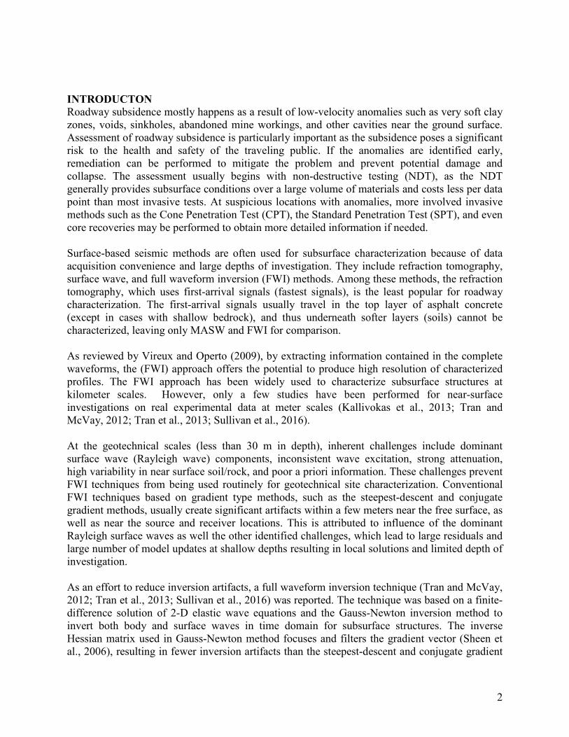
methods. The technique has been successfully applied to real experimental data sets for geotechnical site characterization of soil/rock layers and embedded anomalies (low-velocity zones or voids). However, it requires significant time for data acquisition, as many shots are needed along the receiver array. For example, it takes about 20 minutes to collect data for a road segment of 36 m using 24 receivers and 25 shots at 1.5 m spacing (Sullivan et al., 2016). This requires roadway lane closures for surveys of a few hundred meters, thus interrupting the traffic flow for up to a whole day. To mitigate the traffic interruptions under traditional seismic testing, a new seismic test system is proposed. The system consists of a 24-channel land-streamer and a propelled energy generator (active source). Shown in Fig. 1 was the test configuration for the field experiments. Twenty four receivers at 1.5 m spacing and one shot at 3 m away from the end of receiver array was used. The entire system was moved together quickly from one shot location to the next, and data was recorded shot by shot. The measured seismic dataset was analyzed by the standard multichannel analysis of surface waves (MASW) and a 2-D waveform tomography methods. The results are compared to assess the capabilities of the two methods.

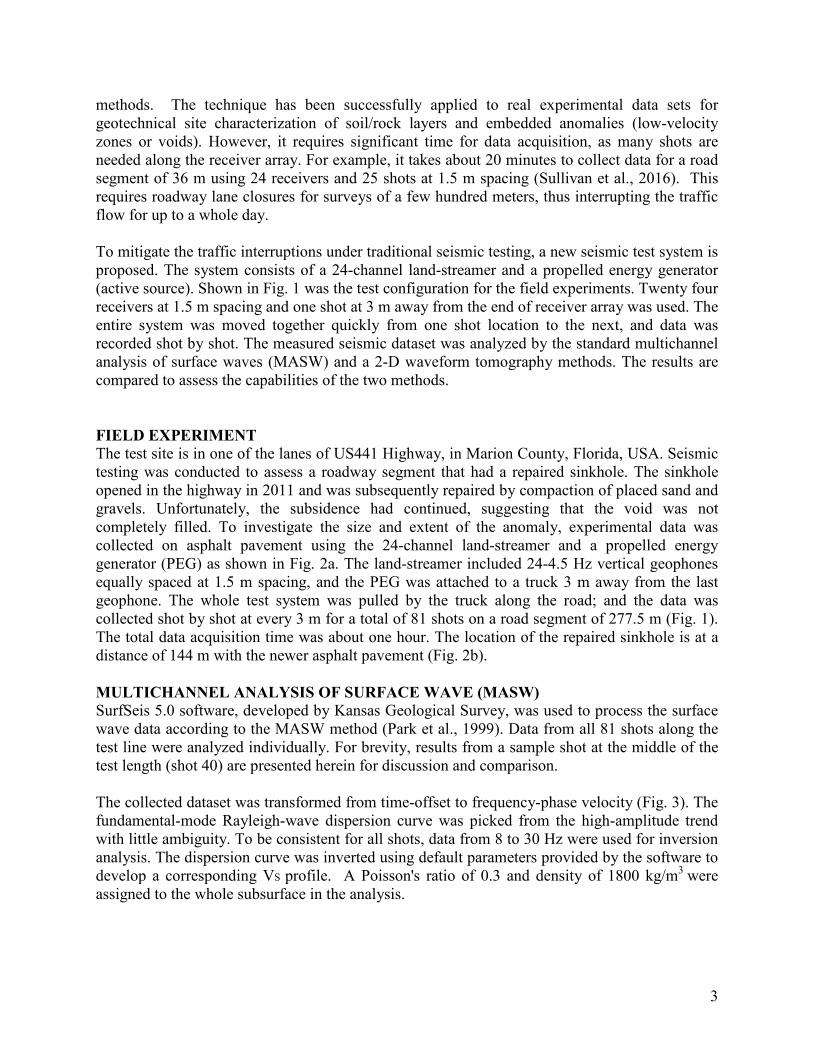
FIELD EXPERIMENT The test site is in one of the lanes of US441 Highway, in Marion County, Florida, USA. Seismic testing was conducted to assess a roadway segment that had a repaired sinkhole. The sinkhole opened in the highway in 2011 and was subsequently repaired by compaction of placed sand and gravels. Unfortunately, the subsidence had continued, suggesting that the void was not completely filled. To investigate the size and extent of the anomaly, experimental data was collected on asphalt pavement using the 24-channel land-streamer and a propelled energy generator (PEG) as shown in Fig. 2a. The land-streamer included 24-4.5 Hz vertical geophones equally spaced at 1.5 m spacing, and the PEG was attached to a truck 3 m away from the last geophone. The whole test system was pulled by the truck along the road; and the data was collected shot by shot at every 3 m for a total of 81 shots on a road segment of 277.5 m (Fig. 1). The total data acquisition time was about one hour. The location of the repaired sinkhole is at a distance of 144 m with the newer asphalt pavement (Fig. 2b). MULTICHANNEL ANALYSIS OF SURFACE WAVE (MASW) SurfSeis 5.0 software, developed by Kansas Geological Survey, was used to process the surface wave data according to the MASW method (Park et al., 1999). Data from all 81 shots along the test line were analyzed individually. For brevity, results from a sample shot at the middle of the test length (shot 40) are presented herein for discussion and comparison. The collected dataset was transformed from time-offset to frequency-phase velocity (Fig. 3). The fundamental-mode Rayleigh-wave dispersion curve was picked from the high-amplitude trend with little ambiguity. To be consistent for all shots, data from 8 to 30 Hz were used for inversion analysis. The dispersion curve was inverted using default parameters provided by the software to develop a corresponding VS profile. A Poisson's ratio of 0.3 and density of 1800 kg/m3 were assigned to the whole subsurface in the analysis.

4

Results of the inversion of the MASW data are shown in Fig. 4. The estimated and measured dispersion curves match well. The depth of the half space (~18 m) was roughly one third of the maximum wavelength of the data used for analysis (~ 53 m). The VS ranged between ~ 250 m/s and 360 m/s, except in the bottom (> 18m) of the half space (VS ~ 500 m/s). VS decreased with increasing depth in the range of ~ 4 m to 11 m. Eighty one 1-D VS profiles from the MASW were combined (3 m separation) to obtain a single 2-D profile shown in Fig. 5. Each 1-D VS profile from the MASW represents the VS profile at the middle of the geophone array. For example, the first VS profile (first shot) is at distance 17.25 m (half of 34.5 m geophone array length), the second VS profile is at distance 20.25 m (3 m away), and so on. Controlling the dominant VS value in the figure is the horizontal mean value, although significant local velocity variations appear within the layers, particularly near the surface. The inverted VS profile includes a stiff layer (VS ~ 300 to 400 m/s) at shallow depth from 0 to 5 m, and a soft layer (VS ~ 150 to 250 m/s) at depth from 5 to 11 m, underlain by stiffer layers with embedded low-velocity zones. FULL WAVEFORM INVERSION The FWI technique (Tran and McVay, 2012; Tran et al., 2013, Sullivan et al., 2016) has been reported for geotechnical site characterization at meter scales. The technique includes forward modeling to generate synthetic wave fields as well as a Gauss-Newton inversion method to update model (soil/rock) parameters until residuals between predicted and measured waveform data are negligible. For the forward modeling, the classic velocity-stress staggered-grid finite difference solution of 2-D elastic wave equations in the time domain (Virieux, 1986) is used in combination with perfectly matched layer (PML) boundary conditions (Kamatitsch and Martin, 2007). The FWI technique (Sullivan et al., 2016) has been modified for land-streamer type data presented herein. To reduce computer time and memory (RAM), forward simulation is conducted for the segment that the PEG and receivers are connected, not for the entire domain. For example, the forward simulation is only conducted for a segment of 37.5 m length for each shot (34.5 length of the geophone array plus 3 m off-end distance of the source as shown in Fig. 1). PMLs are used at the vertical and bottom boundaries of the modeling medium to absorb energy of outgoing waves. Estimated waveform data from the forward simulation are then compared to measured data to extract the 2-D VS profiles by inversion (see Sullivan et al., 2016 for detailed equations). Application to collected data Unlike the conventional test configuration with shots along receivers, the land-streamer type test uses only one shot at the end of receiver array, and thus produces wave fields mostly propagating horizontally from the shot to receivers as Rayleigh waves. Reflected and refracted body wave signals recorded at receivers are very small compared to the Rayleigh wave signals. As both phase and magnitude of the Rayleigh waves are mostly controlled by the S-wave velocity, i.e. the P-wave velocity and mass density contributions are small, it is difficult to extract the P-wave velocity and mass density for the medium. Thus, during inversion analysis, the mass density throughout the model was kept constant at 1800 kg/m3

, and the P-wave velocity was calculated

5

from the S-wave velocity and a Poisson’s ratio of 0.30. This is similar to MASW’s inversion analysis of dispersion data, i.e. the mass density and Poisson’s ratio are assumed constant during the inversion for the whole domain. To obtain acceptable results from waveform analysis of the measured data, this study has addressed inherent challenges of the small scale tomography including dominant surface wave (Rayleigh wave) components, inconsistent wave excitation, high attenuation, poor a priori information, and high variability of near surface 2D soil/rock properties. For instance, Rayleigh wave components produces high sensitivities (i.e. large partial derivatives) which require large model updates near the ground surface. This could result in shallow artifacts and poor resolution of the deeper structures. However, by employing a Gauss-Newton inversion approach, the inverse Hessian matrix focused and filtered the gradient vector which resulted in a reduction of the shallow artifacts. It also partially balanced the model updates throughout entire domain, and thus helped to resolve the deeper structures (Sheen et al., 2006). The issue of inconsistent wave excitation was greatly reduced by employing the propelled energy generator, which applied the same force and signal frequency content at each source location. To account for high attenuation of real measured data, the modeled wave field (estimated data) was corrected by an offset dependent correction factor of the form y(r) = A· rα (Schäfer et al., 2012). Where r is the source-receiver offset and the factor A and exponent α were determined with an iterative least squares inversion, which minimizes the energy of waveform residuals. The values of A and α were estimated at the beginning of the inversion, and kept constant for each inversion run. These values represent an average attenuation as a function of the source-receiver offset for the whole data set recorded by all receivers from all shots. Using the deterministic Gauss-Newton inversion method, appropriate initial models are required to avoid local solutions. To address the issue of poor a priori information, the waveform analysis begins with the low frequency data, which requires a less detailed initial model. Herein, the initial model was established via a spectral analysis of the measured data. As shown in Fig. 3, the energy in the measured wave field is concentrated in a narrow band, at the frequency range of 8 to 50 Hz, with phase velocity from 300 to 500 m/s. The medium depth of 22.5 m was taken the same as that of the MASW results. With the selected range of the velocity and the medium depth, the initial model was established as 1-D model having S-wave velocity increasing with depth from 300 m/s at the surface to 500 m/s at the bottom of the medium. To further avoid local solutions and address the issue of high variability of soil/rock near the ground surface, the waveform analysis was done in sequence of increasing frequencies. Using low frequency data first requires a less detailed initial model, and introducing high frequency data gradually helps to resolve variability in the surface structures. Three inversion runs were performed with central frequencies of 12, 20 and 30 Hz, with the lower frequency run first. The bandwidth for each central frequency was 20 Hz with 10 Hz on each side. For example, at with the central frequency of 12 Hz, measured signals from 2 to 22 Hz were considered but signals lower than 2 Hz or higher than 22 Hz were removed by low and high-pass filtering as shown in Fig. 6.

6

During the inversion, the medium of 22.5 × 277.5 m was divided into 2775 cells of 1.5 × 1.5 m. S-wave velocities of all cells were updated independently during the inversion. Three inversion runs at 12, 20 and 30 Hz were stopped after 13, 30, 29 iterations respectively, at the point where the change of least-squares error is small (less than 1% from one iteration to the next). The complete analysis took about 5 hours on a standard desktop computer. Normalized least-squares error for all 72 iterations of the three runs is shown in Fig. 7, where the error reduces from 1.0 at the first iteration to 0.33 at the final iteration (iteration 72). The observed surface waveforms, the estimated surface waveforms, and residuals associated with the final inverted model are shown in Fig. 8 for shots 1, 15, 30, 45, 60, and 75 along the tested road segment. The observed and estimated data are very similar, and the residuals are small across the entire range of source-receiver offset, except for channels near the source locations. This difference is mostly due to near-field effect, which is not completely handled by the attenuation correction. The final inversion results from the FWI are shown in Fig. 9. The FWI result shows a stiff soil layer (VS ~ 300 to 400 m/s) at shallow depth from 0 to 5 m, and a soft soil layer (VS ~ 120 to 250 m/s) at depth from 5 to 11 m, underlain by highly variable limestone (VS > 600 m/s). Interestingly, it shows a buried low-velocity zone (VS ~ 120 to 150 m/s) at the location of the repaired sinkhole (distance 144 m). There is also a low-velocity anomaly (VS ~ 150 to 200 m/s) at about 80 m distance and 15 m depth, and suggests further investigation by invasive testing (CPT/SPT) is needed. FWI AND MASW COMPARISON Two dimensional, 2-D, VS profiles obtained from the MASW (Fig. 5) and the FWI (Fig. 9) appear similar. They both include a stiff soil layer at depth from 0 to 5 m, a soft soil layer at depth from 5 to 11 m, underlain by a bottom limestone layer. However, the MASW results shows much less variability within the layers. The VS values from the MASW method are muted (i.e., less transition between extreme ends) because they represent averages over large volumes. For instance, each 1-D VS profile from the MASW method is the average shear wave velocity over a distance of 34.5 m (geophone array length). In the case of FWI, the VS values are computed on 1.5 x 1.5 m cell size for 2775 independent values. To better compare the Vs profiles, shown in Fig. 10a are the distance-averaged VS profiles for the entire test length of 277.5 m for the two methods. They are calculated from all 81 1-D Vs profiles for the MASW (10 layers), and VS values of cells along the distance for the FWI at each depth. Apparently, the distance-averaged VS profiles agree quite well, particularly at depths from 0 to 10 m. Shown in Fig. 10b are VS profiles from the MASW and FWI methods at only the repaired sinkhole location (distance 144 m). They are similar from 0 to 8 m depth, and significantly different from 8 to 15 m depth. Again, the discrepancy is because Vs profile from the FWI represents the local values at the repaired sinkhole, whereas VS values from the MASW are the average values over a distance of 34.5 m. The lowest VS value from the FWI is about 120 m/s at the depth of 12 m, suggesting the void may be filled by soft raveled soils.

7

CONCLUSION A new land-streamer seismic test system is presented for assessment of roadway substructures. It includes a 24-channel land-streamer and a propelled energy generator source. The main advantage of using a land-streamer system is that the geophones are not required to be coupled to the tested material and employing only one source location at the end of geophone array, thus allowing translation of whole array and quick testing of long extents of roadway. For instance a seismic survey was conducted along a 277.5 m (916 ft) of roadway with the total data acquisition time of about one hour. The measured seismic dataset was subsequently analyzed by the standard multichannel analysis of surface waves (MASW) and the 2-D full waveform inversion (FWI) methods. The FWI method was able to characterize subsurface structures at high resolution (1.5 x 1.5 m cells) to 22.5 m depth and identify low-velocity anomalies, including one at a repaired sinkhole location. The 2-D Vs profiles from the MASW and waveform tomography methods were shown to be similar with best correlation (MASW and FWI) when the FWI is averaged horizontally over the test length. For the latter, both methods were able to delineate high- and low-velocity soil layers and variable bedrock.

37,5m3m

277,5m

SHOT 2

SHOT 1

SHOT 80

SHOT 81

24 Receivers at 1.5m spacing1,5m

Shot

Receiver

LEGEND

S1

S2

S81

S80

Figure 1. Test configuration used for field experiments

8

Figure 2. Field experiment on US441 Highway, Marion County, Florida

a) Propelled energy generator and land-streamer

b) Repaired sinkhole location with new asphalt

9

Figure 3. Sample dispersion image of shot 40 (velocity in m/s, ~ 50 to 1000, with respect to frequency in Hz, ~ 4 to 50) and picked dispersion curve (white dots).

10

Figure 4. VS profile developed from inversion of the picked dispersion curve (shot 40). Velocity is in m/s, depth is in m. Symbols (dots): picked dispersion curve (data); dashed curve: computed dispersion curve corresponding to starting model; solid curve: dispersion curve corresponding to final solution; dashed stepped lines: starting VS profile; solid stepped lines: final VS profile.

Figure 5. VS profile developed from MASW analysis by combing 81 1-D profiles from individual shots. The first VS profile (first shot) is at distance 17.25 m (half of 34.5 m geophone array length), the last VS profile for shot 81 is at distance 257.25 m.

Distance (m)

Dep

th (m

)

S-Wave

50 100 150 200 250

5

10

15

20 200

300

400

500

11

a) Filtered measured data

b) Corresponding frequency spectra

Figure 6. Sample field experimental data: a) filtered measured data, and b) corresponding frequency spectra for the first shot at distance 37.5 m. Signals lower than 2 Hz or higher than 22 Hz were removed by low- and high-pass filtering.

0 5 10 15 20 250

0.1

0.2

0.3

0.4

0.5

0.6

0.7Measured data

Tim

e (s

)

Receiver Number

0 5 10 15 20 25 30 35 400

50

100

150

Frequency (Hz)

Mag

nitu

de

12

Figure 7. Normalized least squares error versus the inversion iteration number. The error defines the degree of match between the estimated and observed waveforms during the inversion analysis.

0

0.2

0.4

0.6

0.8

1

1.2

0 10 20 30 40 50 60 70 80

Nor

mal

ized

Leas

t Squ

ares

Err

or

Iteration

13

Figure 8. Comparison between observed data and estimated data shots 1, 15, 30, 45, 60, and 75 (left to right)

0 50 100 150 200 2500

0.2

0.4

0.6

Observed dataTi

me

(s)

Receiver position (m)

0 50 100 150 200 2500

0.2

0.4

0.6

Estimated data

Tim

e (s

)

Receiver position (m)

0 50 100 150 200 2500

0.2

0.4

0.6

Residual

Tim

e (s

)

Receiver position (m)

14

Figure 9. VS profile developed from FWI analysis (in m/s) a)

b)

Figure 10. Comparison of VS profiles from MASW and FWI methods: a) distance-averaged VS profiles for the entire test length of 277.5 m and b) VS profiles at repaired sinkhole location (distance 144 m).

Distance (m)

Dep

th (m

)S-Wave

0 50 100 150 200 250

0

5

10

15

20 200

400

600

0

5

10

15

20

25

0 200 400 600

Dept

h (m

)

S- wave velocity (m/s)

Distance-averaged FWI

Distance-averaged MASW

0

5

10

15

20

25

0 200 400 600 800De

pth

(m)

S- wave velocity (m/s)

FWI at 144 m

MASW at 144 m

Repaired sinkhole

15

REFERENCES Kamatitsch D. and Martin R. (2007). An unsplit convolutional perfectly matched layer improved

at grazing incidence for the seismic wave equation: Geophysics; 72(5), SM155–SM167. Kallivokas L.F., Fathi A., Kucukcoban S., Stokoe K.H., Bielak J., Ghattas O. (2013). Site

characterization using full waveform inversion: Soil Dynamics and Earthquake Engineering; 47:62–82.

Park C. B., R. D. Miller, and J. Xia, (1999). Multi-channel analysis of surface wave (MASW): Geophysics, 64, no. 3, 800-808.

Schäfer M., Groos L., Forbriger T. and Bohlen T. (2012). On the Effects of Geometrical Spreading Corrections for a 2D Full Waveform Inversion of Recorded Shallow Seismic Surface Waves: 74th EAGE Conference & Exhibition incorporating SPE EUROPEC 2012Copenhagen, Denmark, 4-7 June 2012.

Sheen D.H., Tuncay K., Baag C. E. and Ortoleva P. J. (2006). Time domain Gauss–Newton seismic waveform inversion in elastic media: Geophysical Journal International; 167: 1373-1384.

Sullivan B., Tran K.T, and Logston B. (2016), “Characterization of Abandoned Mine Voids Under Roadway Using Land-streamer Seismic Waves”, Journal of Transportation Research Board, Vol. 2580, pp 71-79.

Tran K.T., McVay. M., Faraone M., and Horhota D. (2013), Sinkhole Detection Using 2-D Full Seismic Waveform Tomography: Geophysics, 78 (5), R175–R183.

Tran K. T. and McVay M. (2012). Site Characterization Using Gauss-Newton Inversion of 2-D Full Seismic Waveform in Time Domain: Soil Dynamics and Earthquake Engineering; 43: 16-24.

Virieux J. (1986). P–SV wave propagation in heterogeneous media: velocity–stress finite-difference method: Geophysics; 51(4): 889–901.

Vireux J. and Operto S. (2009). An overview of full-waveform inversion in exploration geophysics: Geophysics; 74(6): WCC1-WCC26.