istanbul technical university graduate school of …Çapraz kesici sistem, bir servo motor...
TRANSCRIPT

ISTANBUL TECHNICAL UNIVERSITY GRADUATE SCHOOL OF SCIENCE
ENGINEERING AND TECHNOLOGY
M.Sc. THESIS
JUNE 2013
CROSS-CUTTER SYSTEM LOAD TORQUE ANALYSIS, SYSTEM CONTROL
AND SIMULATION
Baturalp AKSOY
Department of Mechatronics Engineering
Mechatronics Engineering Programme
Anabilim Dalı : Herhangi Mühendislik, Bilim
Programı : Herhangi Program


JUNE 2013
ISTANBUL TECHNICAL UNIVERSITY GRADUATE SCHOOL OF SCIENCE
ENGINEERING AND TECHNOLOGY
CROSS-CUTTER SYSTEM LOAD TORQUE ANALYSIS, SYSTEM CONTROL
AND SIMULATION
M.Sc. THESIS
Baturalp AKSOY
(518101007)
Department of Mechatronics Engineering
Mechatronics Engineering Programme
Anabilim Dalı : Herhangi Mühendislik, Bilim
Programı : Herhangi Program
Thesis Advisor: Asst. Prof. Ali Fuat ERGENÇ


HAZİRAN 2013
İSTANBUL TEKNİK ÜNİVERSİTESİ FEN BİLİMLERİ ENSTİTÜSÜ
DÖNEL BIÇAKLI KESME SİSTEMLERİNDE
YÜK TORKU ANALİZİ, SİSTEM KONTROLÜ VE SİMÜLASYONU
YÜKSEK LİSANS TEZİ
Baturalp AKSOY
(518101007)
Mekatronik Mühendisliği Anabilim Dalı
Mekatronik Mühendisliği Programı
Anabilim Dalı : Herhangi Mühendislik, Bilim
Programı : Herhangi Program
Tez Danışmanı: Yar. Doç. Ali Fuat ERGENÇ


v
Thesis Advisor : Asst. Prof. Ali Fuat ERGENÇ ..............................
Istanbul Technical University
Jury Members : Asst. Prof. Pınar BOYRAZ .............................
Istanbul Technical University
Asst. Prof. Özgür Turay KAYMAKÇI ..............................
Yıldız Technical University
Baturalp Aksoy, a M.Sc. student of ITU Institute of Science student ID 518101007,
successfully defended the thesis entitled “APPLICATION OF A MATRIX
TECHNIQUE FOR DOMINANT POLE PLACEMENT OF DISCRETE-TIME
TIME-DELAYED SYSTEMS ON A CROSS-CUTTER SYSTEM”, which he
prepared after fulfilling the requirements specified in the associated legislations,
before the jury whose signatures are below.
Date of Submission : 3 May 2013
Date of Defense : 11 June 2013

vi

vii
To my family,

viii

ix
FOREWORD
Cross-cutter systems are simple rotary systems that are widely used in the industry to
cut sheet metal, paper and the like with a rotary knife motion. However these
systems present a unique example which has two different movement zones and
native time delay in their speed responses. This thesis takes on the control problem of
this unique system with a different discrete time matrix approach for time delayed
systems.
I would like to present my sincerely thanks to my advisor Asst. Prof. Ali Fuat
ERGENÇ who has helped me in all layers of the problem and the solution.
May 2013
Baturalp AKSOY

x

xi
TABLE OF CONTENTS
Page
FOREWORD ............................................................................................................. ix TABLE OF CONTENTS .......................................................................................... xi ABBREVIATIONS ................................................................................................. xiii
LIST OF TABLES ................................................................................................... xv
LIST OF FIGURES ............................................................................................... xvii
SUMMARY ............................................................................................................. xix ÖZET ........................................................................................................................ xxi 1. INTRODUCTION .................................................................................................. 1
1.1 Purpose of Thesis ............................................................................................... 1 1.2 Introduction of the Cross-Cutter System ............................................................ 1
1.3 System Configuration ......................................................................................... 4
2. SYSTEM ANALYSIS ............................................................................................ 7 2.1 PLC Routine ....................................................................................................... 7 2.2 Obtaining Rotary Knife Mathematical Model ................................................. 10 2.3 Open Loop Root Locus .................................................................................... 14
3. CUTTING OPERATION .................................................................................... 15 3.1 Enacting Forces in Cutting Operation .............................................................. 15
3.2 Rotary Knife Velocity Analysis ....................................................................... 18
3.2.1 Inside the cutting zone : Zones 1 and 2 ..................................................... 18
3.2.2 Inside the catch-up zone: Zone 3 .............................................................. 19 3.3 Load Torque Input Argument .......................................................................... 20 3.4 Integration Into System Model ......................................................................... 22
3.4.1 Case1: Piece length is equal to rotary knife circumference ...................... 25
3.4.2 Case2: Piece length is bigger than the rotary knife circumference. .......... 26 3.4.3 Case3: Piece length is smaller than the rotary knife circumference ......... 27
4. CONCLUSIONS AND RECOMMENDATIONS ............................................. 29 4.1 Practical Application of This Study ................................................................. 29
APPENDICES .......................................................................................................... 33
CURRICULUM VITAE .......................................................................................... 39

xii

xiii
ABBREVIATIONS
MSO : Motion Servo On
MSF : Motion Servo Off
MAJ : Motion Axis Jog
TON : Timer On Delay

xiv

xv
LIST OF TABLES
Page
Table 2.1 : RSLogix 5000 motion blocks used in rotary knife
modelling routine. ................................................................................... 11

xvi

xvii
LIST OF FIGURES
Page
Figure 1.1 : Cross-cutter conveyor system. (View from side) .................................... 1 Figure 1.2 : Cross-cutter system ................................................................................. 2 Figure 1.3 : Rotary knife movements.......................................................................... 2 Figure 1.4 : Piece length sensor function. (View from top). ....................................... 4
Figure 1.5 : Piece length sensors ................................................................................. 4 Figure 1.6 : Allen Bradley Kinetix 6000..................................................................... 5
Figure 1.7 : Allen Bradley Logix 5563 PLC ............................................................... 6 Figure 2.1 : Rotary knife modelling routine ............................................................... 8 Figure 2.2 : Rotary knife velocity trend screenshot. ................................................... 9 Figure 2.3 : Importing and plotting knife velocity trend data into MATLAB. ......... 10
Figure 2.4 : Rotary knife velocity step input response. ............................................ 10 Figure 2.5 : Simulink model for system response comparison ................................. 11
Figure 2.6 : System response comparison ................................................................. 12 Figure 2.7 : Block diagram of rotary knife and controller ........................................ 12 Figure 2.8 : Block diagram of rotary knife and controller ........................................ 13
Figure 2.9 : Open loop root-locus of ........................................................... 14 Figure 3.1: Rotary knife operative variables ............................................................. 15
Figure 3.2: Rotary knife velocity and affecting variables ......................................... 18
Figure 3.3: Rotary knife electric DC motor mathematical model ............................. 22 Figure 3.4: Rotary knife system inertia and friction block ....................................... 22 Figure 3.5: Rotary knife system Simulink model ..................................................... 23
Figure 3.6: Piece length is equal to rotary knife circumference ............................... 25 Figure 3.7: Piece length is bigger than the rotary knife circumference .................... 26
Figure 3.8: Piece length is smaller than the rotary knife circumference ................... 27

xviii

xix
CROSS-CUTTER SYSTEM LOAD TORQUE ANALYSIS, SYSTEM
CONTROL AND SIMULATION
SUMMARY
The cross-cutter system consists of a conveyor belt that is driven by a servo-motor, a
rotary knife that is also driven by a servo-motor and two optical sensors which are
directly positioned above the conveyor belt within a certain distance from the rotary
knife.
The cross cutter system will be modeled along with the load torque that is driven by
the cutting operation. This system will be controlled with a PID controller and
simulations will be conducted to determine cutting efficiency.
The linear velocity of the rotary knife must be equal to the linear velocity of the
conveyor belt within the range where the cutting operation occurs to avoid any strain
and deformation on the material web. This constraint reveals two different movement
zones for the rotary knife: The synchronization move and the make-up move.
The cut length will vary within three different cases depending on the knife velocity
assuming the belt velocity is constant.
If the rotary knife has a constant velocity that is equal to the conveyor belt velocity in
both its movement zones, consequently the cut length of the material will be equal to
the circumference of the rotary knife body.
In the case where the cut length is chosen greater than the rotary knife circumference,
the make up movement must be slower than the belt move to obtain greater length of
material passing under the rotary knife in the same amount of time.
In the case where the cut length is chosen smaller than the rotary knife
circumference, the make up movement must be faster than the belt move to obtain
lesser length of material passing under the rotary knife in the same amount of time.
Test environment of this thesis is the cross cutter system which is located in Control
Engineering Power and Motion Control Laboratory under the name of Rotary Knife
Motion Control Experiment Set.
Both the rotary knife and the conveyor belt servo-motors are driven by Allen-
Bradley Kinetix 6000 Servo Drives which are controlled by inputs from an Allen-
Bradley Logix 5563 PLC. PLC routines are written using RSLogix 5000 Professional
software. All components listed herein are products of Rockwell Automation.
A detailed analysis of acting forces during the cutting operation is conducted and A
PID controller is designed to control the rotary knife velocity. The results are
simulated and error rates are calculated for different piece lenght cases.

xx

xxi
DÖNEL BIÇAKLI KESME SİSTEMLERİNDE YÜK TORKU ANALİZİ,
SİSTEM KONTROLÜ VE SİMÜLASYONU
ÖZET
Çapraz kesici sistem, bir servo motor tarafından tahrik edilen bir konveyör, aynı
zamanda, bir servo motor ve belli bir mesafede olan taşıyıcı kayış üzerinde
konumlandırılmış iki optik sensör ve servomotor ile tahrik edilen bir dönel bıçaktan
oluşmaktadır.
Kesici sistem ve kesme operasyonundan doğan yük torku bu tezde modellenecek ve
bir PID kontrolör aracılığıyle kontrol edilecektir. Kontrol edilen sistemin
simulasyonu yapılarak parça kesme işlemindeki hata oranları bulunacaktır.
Dönel bıçak doğrusal hız kesme işlemi malzeme tabakası üzerinde herhangi bir yük
ve deformasyonunu önlemek için belirlenmiş senkronizasyon aralığında konveyör
bandın doğrusal hızına eşit olması gerekir. Bu kısıtlama dönel bıçağı için iki farklı
hareket bölgesi ortaya koymaktadır. Senkronizasyon hareket ve yetişme hareketi.
Kesme uzunluğu konveyor bandın hızı sabit kabul edilirse bıçak hızına bağlı olarak
üç farklı durumda incelenir.
Dönel bıçak her iki hareket bölgesinde verilen konveyör bant hızına eşit sabit bir
hızda ise, malzemenin kesme uzunluğu dönel bıçak gövdesinin çevresine eşit
olacaktır.
Kesme uzunluğu dönel bıçak çevresinden daha büyük seçildiği durumda yetişme
hareketinin, aynı zaman aralığında dönel bıçak altından geçen malzemenin daha uzun
olması için kayış hareketinden daha yavaş olması gerekir.
Kesme uzunluğu dönel bıçak çevresinden daha küçük seçildiği durumda ise yetişme
hareketinin, aynı zaman aralığında dönel bıçak altından geçen malzemenin daha kısa
olması için kayış hareketinden daha hızlı olması gerekir.
İki fiber optik sensör malzeme uzunluğu geribildirimini sağlamak için dönel bıçaktan
önce konumlandırılmıştır. Sensörlerden gelen farklı geri bildirimlere göre konveyör
bant üzerindeki işaretler uzunlukları atamak için kodlanabilir.
Bu tezin test ortamı Dönel Bıçak Hareket Kontrol Deney Seti adı altında Kontrol
Mühendisliği Güç ve Hareket Kontrol Laboratuvarında bulunan dönel bıçaklı kesici
sistemidir.
Dönel bıçak ve konveyör bant servomotorları Allen-Bradley Kinetix 6000 Servo
Sürücüler tarafından tahrik edilmektedir. Sürücü girişleri Allen-Bradley Logix 5563
PLC tarafından kontrol edilir. PLC rutinleri RSLogix 5000 Professional yazılımı
kullanılarak yazılır. Burada listelenen tüm bileşenleri Rockwell Automation
ürünüdür.
Kesme operasyonu sırasında oluşan güçlerin detaylı bir analizi yapılmıştır ve dönel
bıçak hızını kontrol etmek için bir PID kontrolör tasarlanmıştır.
Sonuçlar simülasyona sokularak farklı parça boyları için kesme durumları
incelenerek hata oranları hesaplanmıştır.

xxii

1
1. INTRODUCTION
1.1 Purpose of Thesis
This thesis will take on a cross-cutter system with a rotary knife and a conveyor belt
to obtain a correct mathematical model of the comlete system motion and
subsequently apply a matrix technique for dominant pole placement in this time-
delayed system.
1.2 Introduction of the Cross-Cutter System
The cross-cutter system consists of a conveyor belt that is driven by a servomotor, a
rotary knife that is also driven by a servomotor and two optical sensors, which are
directly positioned above the conveyor belt within a certain distance from the rotary
knife.
Figure 1.1 : Cross-cutter conveyor system. (View from side)
The conveyor belt has 3 axis points that are positioned triangularly with respect to
each other. This is a common disposition which facilitates the removal of the belt
when and if necessary. The rightmost pulley in Figure 1.1, depicted as is driven
by a servo-motor which will allow velocity ( ) feedback and control. The other two
2
pulleys which are depicted in Figure 1.1 as and are idle rollers without a motor
in the setup this thesis will use.
A photo of the system is given in Figure 1.2.
Figure 1.2 : Cross-cutter system
The rotary knife is driven by a servomotor and consists of a circular body and a
triangular bulge on the outer diameter representing the cutter-knife. This body rotates
around the servo-motor axis to symbolically cut the web of material carried by the
conveyor belt as depicted in Figure 1.2.
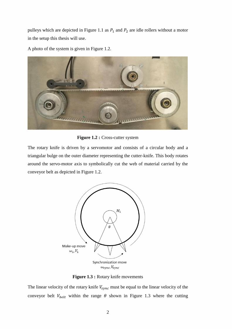
Figure 1.3 : Rotary knife movements
The linear velocity of the rotary knife must be equal to the linear velocity of the
conveyor belt within the range shown in Figure 1.3 where the cutting

3
operation occurs to avoid any strain and deformation on the material web. This
constraint reveals two different movement zones for the rotary knife: The
synchronization move and the make-up move.
The cut length will vary within 3 different cases depending on the knife velocity
assuming the belt velocity is constant.
Case 1:
If the rotary knife has a constant velocity that is equal to the conveyor belt
velocity in both its movement zones (make up move and synchronization
move), consequently the cut length of the material will be equal to the
circumference of the rotary knife body.
→
(1.1)
Case 2:
In the case where the cut length is chosen greater than the rotary knife
circumference , the make up movement must be slower than the belt move to
obtain greater length of material passing under the rotary knife in the same amount of
time .
→
(1.2)
Case 3:
In the case where the cut length is chosen smaller than the rotary knife
circumference , the make up movement must be faster than the belt move to
obtain lesser length of material passing under the rotary knife in the same amount of
time .
→
(1.3)
Two fiber optical sensors are positioned before the rotary knife to allow material
length feedback based on markings on the material web as seen in Figure 1.4. The
feedback from the sensors could be encoded to assign lenghts to different feedbacks.

4
To give an arbitrary example: Single marker on the right could mean whereas
double markers could mean and single marker on the left could mean .
Figure 1.4 : Piece length sensor function. (View from top).
A photo of the sensors is given in Figure 1.5.
Figure 1.5 : Piece length sensors
1.3 System Configuration
Test environment of this thesis is the cross-cutter system, which is located in Control
Engineering Power and Motion Control Laboratory under the name of Rotary Knife
Motion Control Experiment Set.
Both the rotary knife and the conveyor belt servo-motors are driven by Allen-
Bradley Kinetix 6000 Servo Drives as seen in Figure 1.6.

5
Figure 1.6 : Allen Bradley Kinetix 6000
These drives are controlled by inputs from an Allen-Bradley Logix 5563 PLC which
is shown in Figure 1.7.

6
Figure 1.7 : Allen Bradley Logix 5563 PLC
PLC routines are written using RSLogix 5000 Professional software. All components
listed herein are products of Rockwell Automation.

7
2. SYSTEM ANALYSIS
2.1 PLC Routine
A simple main routine is written within RSLogix 5000 as seen in Figure 2.1 using
ladder programming to give speed inputs to the rotary knife servo-motor and to
obtain a closed loop system response for this input. Programming blocks used in the
routine are motion blocks, timer blocks and positive/negative switch blocks as seen
in Table 2.1.
Table 2.1 : RSLogix 5000 Motion Blocks Used In Rotary Knife Modelling Routine
Code Name Description
MSO Motion Servo On Activates the drive amplifier and servo loop for
the axis.
MSF Motion Servo Off Deactivates the drive output and servo loop for the
axis.
MAJ Motion Axis Jog Moves an axis at a constant speed until stop input
received.
TON Timer On Delay Non-retentive timer that accumulates time when
enabled.
Rotary knife servo-motor is defined within the motion group as AXIS_02_Knife.
Two boolean variables named “ServoOn” and “start” are defined to act as software
switches in the routine. Two other variables “timer” and “timer2” are defined to be
used in timer (TON) motion blocks. Lines of the ladder routine are referred as
“rungs”.
A velocity trend is defined to track both “AXIS_02_Knife.ActualVelocity” and
“AXIS_02_Knife.CommandVelocity” signals to obtain a graph representation of the
input and output velocity values. This trend is triggered by the routine in Figure 2.1.
The movement of the rotary knife is sampled using sample size in this trend.
Rotary knife axis is controlled by a velocity gain PI controller within the PLC. An
arbitrary proportional gain and an arbitrary integral gain
are set within the PI controller for the AXIS_02_Knife.

8
Figure 2.1 : Rotary knife modelling routine
The routine in Figure 2.1 is explained step by step as follows:
When the soft switch “ServoOn” is closed, the drive amplifier and the servo loop for
the rotary knife servo-motor axis (AXIS02_Knife) is activated by the MSO motion
block.

9
When the soft switch “ServoOn” is open, the MSF block is active. This means the
servo loop is deactivated.
When the “start” switch is also closed alongside with “ServoOn” switch, the first
timer which counts towards is enabled. At the same time, MAJ motion
block on rung 3 is activated. This block moves the depicted AXIS02_Knife at a
constant speed given as within the block.
In rung 3 MAJ motion block has a switch before it with the variable “timer.DN”
which is the DN bit of the first TON block that is used. This switch ensures that
when the timer has accumulated the given and the DN bit is enabled, the
MAJ motion block on rung 3 is deactivated.
The same bit “timer.DN” switches the MAJ motion block on rung 4 enabling it.
When enabled MAJ motion block on rung 4 moves the depicted AXIS02_Knife at a
constant speed given as within the block.
The same bit “timer.DN” switches the second timer block TON on rung 5 which also
counts towards 1000ms after which it enables the “timer2.DN” bit.
The “start” bit is used to trigger the start of the velocity trend and the “timer2.DN”
bit is used to trigger the stop of velocity trend.
As a result of the routine the trend in Figure 2.2 is obtained and exported to
MATLAB environment for calculations.
Figure 2.2 : Rotary knife velocity trend screenshot.

10
Exported values are plotted in MATLAB using the m file depicted in Figure 2.3.
Figure 2.3 : Importing and plotting knife velocity trend data into MATLAB.
2.2 Obtaining Rotary Knife Mathematical Model
Plotted rotary knife velocity response shows actual velocity against the input velocity
in Figure 2.4. This plot and the imported data will be used to obtain a mathematical
model for the rotary knife servo-motor and drive.
Figure 2.4 : Rotary knife velocity step input response.
Overshoot and peak time
is obtained from the imported data as
following:
(2.1)
23 23.5 24 24.5 25 25.5
0
10
20
30
40
50
60
70
80
90
100
110
120
X: 23.32
Y: 65.81
time
velo
city
velocity response
Actual Velocity
Input Velocity

11
(2.2)
(
)
√ ( )
(2.3)
√
(2.4)
The system response also has a time delay.
Applying these values into the standard form of a second order system:
(2.5)
This second order system is compared to the actual measured data and to the output
of MATLAB system identification tool using the simulink model in Figure 2.5.
Figure 2.5 : Simulink model for system response comparison
The result plot of this simulink model is shown in Figure 2.6.

12
Figure 2.6 : System response comparison
Observed and plotted response belongs to the system of rotary knife servo-motor
drive and PI controller. This system could be expressed using the block diagram in
Figure 2.7.
Figure 2.7 : Block diagram of rotary knife and controller
The system response obtained from the rotary knife velocity trend will be called
as depicted in Figure 2.8.
1 1.05 1.1 1.15 1.2 1.25
x 10-3
100
120
140
160
180
200
220
Time
Velo
city
System Response
Measured System Response
Input Velocity
Gm
k (s) Proposed System
MATLAB System Identifier

13
Figure 2.8 : Block diagram of rotary knife and controller
The transfer function for the rotary knife system will be derived from the
obtained system response using the controller values proportional gain
and integral gain
from the PI controller .
(2.6)
From the block diagram in Figure 2.8:
(2.7)
From here we derive as following:
( )
(2.8)
As arbitrary values, proportional gain and integral gain
are set within the PI controller.
Using these values;
(2.9)
Using Equation (2.5) and Equation (2.9) the transfer function of the rotary knife is
obtained as following:

14
(2.10)
Obtained transfer function represents a second order system with two following open
loop poles:
(2.11)
2.3 Open Loop Root Locus
Open loop root-locus is represented in Figure 2.9. As one of the poles is more than
100 times far left in the root-locus, its effect rapidly decays and neglectible.
Therefore, the system will behave similar to a first order system. The first root seen
in Equation 2.11 represents the electrical section of the system while the second root
, mechanical section.
Figure 2.9 : Open loop root-locus of
-90 -80 -70 -60 -50 -40 -30 -20 -10 0-1.5
-1
-0.5
0
0.5
1
1.5
Root Locus Editor for Open Loop 1 (OL1)
Real Axis
Imag A
xis

15
3. CUTTING OPERATION
3.1 Enacting Forces in Cutting Operation
Figure 3.1: Rotary knife operative variables
To be able to understand the forces acting upon the rotary knife and the material web
that is being cut, Figure 3.1 has been drawn.
In Figure 3.1, the inner circle represents the rotary knife body and the outer circle is
the blade tip movement circumference.

16
Three arrows pointing towards the material web represent the cutting blade and its
various positions upon the material web. These three positions are pointing to three
point of interests for the movement.
The first one on the left is the first point that the blade tip touches the material web
and the acting cutting force is met with a resistance. This point is detoned as
for future use in calculations.
The second position of the blade is the origin position and the third one is the
point where the blade leaves the material web.
The radius of the blade tip movement circumference, is denoted as and the angle
between the first cut position and the origin position of the blade is denoted as .
(
) (3.1)
is calculated below to be used in Equation 3.10.
(3.1)
(3.2)
(3.3)
√ (3.4)
√
(3.5)
Inside the cutting zone, the linear velocity of the rotary knife must be equal to the
linear velocity of the material web to avoid any deformation to the material web.
(3.6)
The cut begins at the point and continues until the blade reaches the origin
point As the material web moves together with the blade tip during the cutting
operation, the cut movement is stritctly vertical.

17
The movement of the blade tip, enacts as shear stress over the cross section of
the material which is denoted as . The thickness of the material is denoted
as and the width of the material web is denoted as .
The shear stress causes a failure in the material when it is equal or greater than
the ultimate tensile stress of the material .
The material is chosen to allow a brittle failure and an ideal cut.
The reactive force from the material web creates a load torque that enacts as an
input into the rotary system from the time the cut begins at to the time blade
reaches the origin point
(3.7)
(3.8)
(3.9)
is calculated dependent to the ultimate tensile strength , the blade tip
movement radius and the cross section of the material being cut .
√
(3.10)
√
(3.11)

18
3.2 Rotary Knife Velocity Analysis
Figure 3.2: Rotary knife velocity and affecting variables
The cutting movement has 3 different zones: the first two zones: Zone 1 and Zone 2,
are inside the actual cutting zone, the third one: Zone 3, is the catch-up zone.
3.2.1 Inside the cutting zone : Zones 1 and 2
Linear speed at the tip of the blade is denoted as:
(3.12)
The horizontal component of the blade tip speed is calculated in zones 1 and 2 in
different ways.
In zone 2, the actual position angle is used to denote the speed equation.
(3.13)
In zone 1, the angle between the origin point o and the blade position can be denoted
as . Therefore, the blade tip speed is calculated as:

19
(3.14)
At this point, two equations become equal as a result of cosine function’s
trigonometric property:
(3.15)
As a result, in both zones 1 and 2 the blade tip speed’s horizontal component is equal
to:
(3.16)
Inside the cutting zone, the the horizontal component of the blade tip speed must
be equal to the material web speed .
(3.17)
(3.18)
3.2.2 Inside the catch-up zone: Zone 3
Inside the catch-up zone, angular distance to be covered is , therefore the
catch-up time is calculated as seen in Equation 3.19.
(3.19)
In this zone, the piece lenght will determine the rotary knife speed as the aim is to
catch-up just in time to cut the end of the piece.
Therefore the catch-up time is also the duration in which the conveyor belt covers
the distance between the end of the piece and the point . This distance could be
denoted as .
(3.20)
Using Equation 3.19 and Equation 3.20,

20
(3.21)
Where
,
(3.22)
(3.23)
(
)
√ (3.24)
3.3 Load Torque Input Argument
Input load torque is calculated in relation to material thickness and blade travel inside
the material.
The blade travel is calculated in Equation 3.25:
(3.25)
This thesis will assume that the load torque will be proportional to blade travel inside
the material. Therefore,
(3.26)
(3.27)
Input load torque should be saturated between cutA and 2pi as these are the limits to
the cut zone.
Fourier series approach is used to saturate the load torque value:

21
∑ (
)
∑ (
)
(3.28)
Where coefficients are,
∫
(3.29)
∫
(3.30)
∫ (
)
(3.31)
∫ (
)
(3.32)
∫ (
)
(3.33)
∫ (
)
(3.34)
The fourier series solution, while useful to saturate between required points, is very
slow and cumbersome. Therefore another method for saturation is used:
√
(3.35)

22
3.4 Integration Into System Model
Figure 3.3: Rotary knife electric DC motor mathematical model
In Figure 3.3 depicted is a mathematical model of an electrical DC motor. To inlcude
the obtained load torque resulting from the cutting operation into the simulink
model, the inertia and friction block must be considered. As seen in Figure 3.3, load
torque input is affecting the system before the inertia and friction block.
The inertia and friction block must be seperated from the obtained system
seen in Equation 2.10, to form a simulink model where the load torque and its
effect on the system could be observed.
To seperate the inertia and friction block, the following method is applied:
Figure 3.4: Rotary knife system inertia and friction block
As seen in Figure 3.4,
(3.36)
(3.37)

23
Transfer function of the rotary knife motor without the inertia and friction coefficient
are obtained as seen in Equation 3.38
( ) (3.38)
Motor inertia and friction coefficient are given as follows:
(3.39)
Using Equation 2.10 and Equation 3.38, Model of the motor is obtained as seen
in Equation 3.40.
( )
(3.40)
Using the transfer function and the mathematical model of the DC electric motor,
a MATLAB Simulink model of the rotary knife system is obtained as seen in Figure
3.5.
Figure 3.5: Rotary knife system Simulink model
A bigger representation of Figure 3.5 is available as Appendix B.
In the depicted model for simulation, the reference is given differently in two
different working zones, the cutting zone and the catch-up zone.
Inside the catch-up zone, the reference is given as in Equation 3.18:
and
inside the cutting zone;

24
The reference is given as in Equation 3.24:
(
)
√
The reference input is given into the PID controller, which is designed according to
empirical optimal settling time in Mathematica as seen in Appendix E.
The control signal is admitted into the system transfer function and load torque input
is received just before the inertia and friction block. The output is integrated to
calculate the position value as .
The load torque input is calculated using the Equation 3.11, and saturated using
Equation 3.35. This input is being effective starting from point to the origin
point as seen in Figure 3.2.
Actual cutted piece length is also calclulated within the simulation by integrating the
conveyor belt speed, thus multiplying simulation time with the speed to obtain the
piece length.
Three different cases are simulated with the denoted model.

25
3.4.1 Case1: Piece length is equal to rotary knife circumference
Figure 3.6: Piece length is equal to rotary knife circumference
As the piece length is equal to the rotary knife circumference, the speed in the catch-
up zone and cutting zone are equal. The effect of the load torque (in red) could be
observed in Figure 3.6.
The simulated actual cut piece length has an error of 0.23% in this case.

26
3.4.2 Case2: Piece length is bigger than the rotary knife circumference.
Figure 3.7: Piece length is bigger than the rotary knife circumference
As the piece length is bigger than the rotary knife circumference, the speed in the
catch-up zone is slower than the speed in cutting zone. The effect of the load torque
(in red) could be observed in Figure 3.7.
The simulated actual cut piece length has an error of 0.14% in this case.
0 0.5 1 1.5 2 2.5 3 3.5 4 4.5 50
1
2
3
4
5
6
7
Time
Velocity
Position
Load Torque
3.5 3.6 3.7 3.8 3.9 4 4.1 4.2 4.3 4.4 4.50
1
2
3
4
5
6
7
Time
Velocity
Position
Load Torque

27
3.4.3 Case3: Piece length is smaller than the rotary knife circumference
Figure 3.8: Piece length is smaller than the rotary knife circumference
As the piece length is smaller than the rotary knife circumference, the speed in the
catch-up zone is faster than the speed in cutting zone. The effect of the load torque
(in red) could be observed in Figure 3.8.
The simulated actual cut piece length has an error of 1.07% in this case.
0 0.5 1 1.5 2 2.5 3 3.5 4 4.5 50
1
2
3
4
5
6
7
8
9
Time
Velocity
Position
Load Torque
2.5 2.6 2.7 2.8 2.9 3 3.1 3.2 3.3 3.4 3.50
1
2
3
4
5
6
7
8
9
Time
Velocity
Position
Load Torque

28

29
4. CONCLUSIONS AND RECOMMENDATIONS
This study has obtained and analyzed a mathematical model of the cross-cutter
system, successfully controlled the rotary knife movements in two different operation
zones and proved an alternative to cam profile operation.
4.1 Practical Application of This Study
This study could be applied in the industry to cross-cutter rotary knife systems to
obtain more efficient and delicate cutting operations. This improvement could save
costs on reduced wastage. The study also could help realize faster systems with high
production speeds without compromising security. As the system proves an
alternative to cam profile operation, usage of such a control system could cut down
operational costs that would be necessary to change cam profiles according to piece
length and system speed.

30

31
REFERENCES
Hibbeler, Russell C. (2010). Mechanics of materials, Prentice hall; 8 edition (April
1, 2010).
ROCKWELL AUTOMATION. (2005). RSLogix 5000 motion user guide, USA.
Kreyszig, E. (2011). Advanced engineering mathematics, Wiley; 10 edition (August
16).
Ogata, K. (1995). Discrete Time Control Systems, Prentice Hall, 2nd edition,
(January 19).
Nise, N.S. (2010). Control Systems Engineering, Wiley; 6 edition (December 14).

32

33
APPENDICES
APPENDIX A: MATLAB m.file for system modelling
APPENDIX B: MATLAB Simulink Model for the Cross-Cutter System Simulation
APPENDIX C: MATLAB m.file for Cross-Cutter System Simulation
APPENDIX D: MATLAB m.file for Fourier series expansion function
APPENDIX E: Mathematica code for PID controller design

34
APPENDIX A syms s Kp = 255.14368 ; Ki = 20 ;
A = xlsread('b.xlsx') ; plot(0.001*A(:,1),A(:,2),0.001*A(:,1),A(:,3)) grid on
Gce = 31011.86 / ( s^2 + 121.1979*s + 31011.86 ) ; Gpi = ( Kp*s + Ki ) / s ;
G = Gce/(Gpi*(1-Gce));

35
APPENDIX B
MATLAB Simulink Model for the Cross-Cutter System Simulation

36
APPENDIX C
clear all; clc
% Motor Parameters % J = 0.000026 ; B = 0.001 ;
% Load Parameters % Vbelt = 50 ; % (mm/s) p = 50 ; % (mm) parça uzunluğu R = 20 ; % (mm) h = 1 ; % (mm) malzeme kalinligi d = 2 ; % (mm) malzeme genisligi sigmaUTS = 0.05 ; % (MPa) celik: 615.4 t=0.001;
% Load Torque calculation % Tl = 10^-3* ( sigmaUTS*(R^2)*d ) / sqrt( ( 2*R/h )-1 ) ; % (Nm)
%cut duration angle% alpha = acos( (R-h)/R ); %(radians) cutA = 6.28 - alpha ; %(radians) % cut completed from point cutA to zero
%Intermeediate variables% wbelt=Vbelt/R; L = sqrt(h*(2*R-h)); t_cut = 2*L/Vbelt; t_catch = (p-2*L)/Vbelt; Ky = R*(2*pi()-2*alpha)/(p-2*L); %catch-up zone constant => Vk=Vb*Ky

37
APPENDIX D
function y = fourier(theta)
A0 = 0.00102845;
y = 0;
for n=3:1:1000
An = (1/2*pi)*( (0.2432 *( sin(3*n)- sin(3.14*n)) )/n + (1/(n^2-
4))*(-0.143061 *cos(3*n)+0.00163087*cos(3.14*n)-
0.245804*n*sin(3*n)+0.255999*n*sin(3.14*n)));
Bn = ( 1/ ( 2*n* (n^2-4) )
)*(pi*((0.9728+0.00260359*n^2)*cos(3*n)+(-0.9728-
0.0127987*n^2)*cos(3.14*n)-
0.143061*n*sin(3*n)+0.00163087*n*sin(3.14*n))) ;
y1= An*cos(n*pi*theta/(2*pi)) + Bn*sin(n*pi*theta/(2*pi));
y=y1+y; end y = y+A0;

38
APPENDIX E

39
CURRICULUM VITAE
Name Surname: Baturalp AKSOY
Place and Date of Birth: İstanbul, 1987
Address: Zekeriyaköy Basın Yayın Sitesi, Hanımeli Sokak No:
13 Sarıyer İstanbul
E-Mail: [email protected]
B.Sc.: ITU Control Engineering
Professional Experience: Türk Telekom R&D (2012-present)
Ford Otosan Product Development (2010-2012)