irvine 29 may 2003 linear response theory & kubo’s formula...

Irvine 29 May 2003 1

Linear Response Theory

& Kubo’s Formula

for Electronic Transport

Jean BELLISSARD 1 2

Georgia Institute of Technology, Atlanta,&

Institut Universitaire de France

Collaborations:

H. SCHULZ-BALDES (T.U. Berlin, Germany)

D. SPEHNER (Essen, Germany)

R. REBOLLEDO (Pontificia Universidad Catolica de Chile)

H. von WALDENFELS (U. Heidelberg, Germany)

1Georgia Institute of Technology, School of Mathematics, Atlanta, GA 30332-01602e-mail: [email protected]


Main ReferencesD. Spehner, Contributions a la theorie du transport electronique,dissipatif dans les solides aperiodiques, These, 13 mars 2000, Toulouse.

J. Bellissard, Coherent and dissipative transport in aperiodic solids,in Dynamics of Dissipation, pp. 413-486, Lecture Notes in Physics, 597, Springer (2002).P. Garbaczewski, R. Olkiewicz (Eds.).

Content

1. Linear Response Theory: Heuristic Background

2. Transport Cœfficients

3. Kubo’s Formula

WarningThis lecture gives a heuristic discussion of problems posed by

the linear response theory in view of a more rigorous study.

It does not intend to give mathematically rigorous results.


I - Linear Response Theory:

Heuristic Background


Linear ResponseExperiments show that if a force ~F is imposed to asystem, its response is a current ~j vanishing as theforce vanishes. Thus for ~F small

~j = L · ~F + O( ~F 2) ,

Here L is a matrix of transport cœfficients.

Examples:

1. Fourier’s law: a temperature gradient produces aheat current ~jheat = −λ~∇T .

2. Ohm’s law: a potential gradient (electric field) pro-

duces an electric current ~jel = −σ~∇V .

3. Fick’s law: a density gradient produce a flow ofmatter ~jmatter = −κ~∇ρ.

-What is the domain of validity ?-What happens for quantum systems ?


A No-Go Theorem: Bloch’s oscillationsIf H = H∗, the one-electron Hamiltonian, is boundedand if ~R = (R1, · · · , Rd) is the position operator (self-adjoint, commuting coordinates), the current is

~J = const.ı

~[H, ~R] ,

Adding a force ~F at time t = 0 leads to a new evolutionwith Hamiltonian HF = H − ~F · ~R. The 0-frequencycomponent of the current is

~j = limt→∞

∫ t

0

ds

teısHF/~ ~J e−ısHF/~ ,

Simple algebra shows that (since ‖H‖ < ∞)

~F ·~j = const. limt→∞

H(t) − H

t= 0 ,

WHY ?This is called Bloch’s Oscillations


DissipationDissipation is the loss of information experienced bythe system observed as the time goes on

Second Principle of Thermodynamics

Clausius-Boltzman entropy

The sources of dissipation can take various aspects

1. External noise random in time

2. Exchange with a thermal bath(reservoir with infinite energy)

3. Collisions/interactions with other particles

4. Loss of energy at infinity (infinite volumes)

5. Chaotic motion: sensitivity to initial conditionsKolmogorov-Sinai entropy

6. Quantum measurement (wave function collapse)

7. Quantum Chaos: the Hamiltonian behaves like arandom matrix. Voiculescu entropy .


Length, Time & Energy Scales

1. Length scales:

• Scattering length: range of interactions betweencolliding particles.

• Mean free path: minimum distance between col-lisions

• Mesoscopic scale: minimum size for the systemto reach a local thermodynamical equilibrium.

• Sample size

2. Times scales:

• Scattering time

• Collision time: time between two consecutivecollisions

• Relaxation time: time for a mesoscopic size torelax to equilibrium

• Mesurement time

• Other times: Heisenbeg times ~/∆E , · · ·

3. Energy scales


Exchanges of Limits

1. Infinite volume limit & low dissipation limit:

• Usually

mean free path � sample size

(i) infinite volume limit (ii) low dissipation limit.

• In nanoscopic systems linear response may fail !The resistivity of a molecule is meaningless !

2. Zero external force limit & large time measure-ment limit:

• in solids~

eV≈ 10−12 − 10−15 s. � measurement time

(i) infinite measurement time limit(ii) low external field.

• In pico-femtosecond laser experiments, failuresof linear response theory are observed.


II - Transport Cœfficients


Local Equilibrium Approximation

• Length Scales:

` � δL � L

` is a typical microscopic length scaleL the typical macroscopic length scale.Then δL is called mesoscopic.

• Time Scales:

τrel � δt � t

τrel is a typical microscopic time scalet the typical macroscopic time scale.Then δt is called mesoscopic.

• The system is partitionned into mesoscopic cellsthe time is partitionned into mesoscopic intervals.

• Mesoscopic cells are completely open systemsAfter a time O(δt) they return to equilibrium.


• Let H be the Hamiltonian of the part of the subsys-tem contained in the mesoscopic cell located at ~x attime t.

• Let X1 = H, X2 · · · , XK be a complete family offirst integral, namely observables commuting withthe Hamiltonian.

• Let Q(~x, t) be the set of indices labeling a commoneigenbasis of the Xα’s: it is the set of microstatesof the system contained in the mesoscopic cell.

• If P(~x,t)(q) denotes the Gibbs probability of the mi-

crostate q ∈ Q(~x, t), its Boltzman entropy is givenby

S(P) = −kB

∑

q∈Q(~x,t)

P(~x,t)(q) ln P(~x,t)(q)

• The maximum entropy principle gives Lagrangemultipliers T (~x, t), F2(~x, t), · · · , FK(~x, t) calledconjugate variables. (In the following F1 = 1)


• The Gibbs state for the mesoscopic cell centered at~x ∈ R

d at time t is:

P(~x,t)(q) =1

Z(~x, t)e−

∑Kα=1 Fα(~x,t) Xα(q)

kBT (~x,t)

• The average values of the first integrals are

δXα(~x, t) =∑

q∈Q(~x,t)

P(~x,t)(q) Xα(q) .

• The volume of the cell δV (~x, t) = δV is mesoscopicand chosen constant in space and time.

• Then δXα(~x, t) = O(δV ) and the local density ofXα is

ρα(~x, t) =δXα(~x, t)

δV.

• Under an infinitesimal change of equilibrium the en-tropy changes as TdS =

∑

α FαdδXα


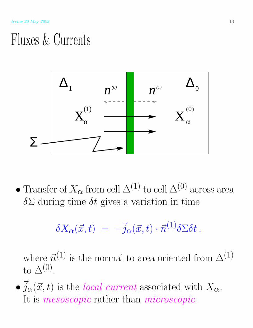
Fluxes & Currents

∆ 1 ∆ 0

X(1)

α

(0)

αX

Σ

n n(0) (1)

• Transfer of Xα from cell ∆(1) to cell ∆(0) across areaδΣ during time δt gives a variation in time

δXα(~x, t) = −~jα(~x, t) · ~n(1)δΣδt .

where ~n(1) is the normal to area oriented from ∆(1)

to ∆(0).

•~jα(~x, t) is the local current associated with Xα.It is mesoscopic rather than microscopic.


• Since Xα is conserved under evolution the balanceleads to the continuity equation

∂ρα

∂t(~x, t) + ~∇ ·~jα(~x, t) = 0 .

• The entropy density is s = δSδV

The entropy variation is then given by

∂s

∂t=

K∑

α=1

Fα

T

∂ρα

∂t.

• The current entropy is define through

~js(~x, t) =

K∑

α=1

Fα

T~jα(~x, t) .

• The entropy production rate is then

ds

dt=

∂s

∂t+ ~∇ ·~js =

K∑

α=1

~∇

(

Fα

T

)

~jα(~x, t) .

and is positive thanks to the 2nd Principle.


Linear Response

• A variation of the Fα/T ’s produces currents.In the local equilibrium approximation

~jα =

K∑

β=1

Lα,β~∇

(

Fβ

T

)

+ O

{

∣

∣

∣

∣

~∇

(

Fβ

T

)∣

∣

∣

∣

2}

– The Lα,β’s are d × d matrices calledOnsager cœfficients.

– The gradient of Fα/T is an affinity.It plays a role similar to forces.

• By 2nd Principle, the positivity of entropy produc-tion rate implies

L = ((Lα,β))Kα,β=1 ⇒ L + Lt ≥ 0

• Reciprocity Relations: if, under time reversal

symmetry, XαTR→ εαXα then

Lβ,α(parameters) = εα εβ Ltα,β(TR-parameters) .


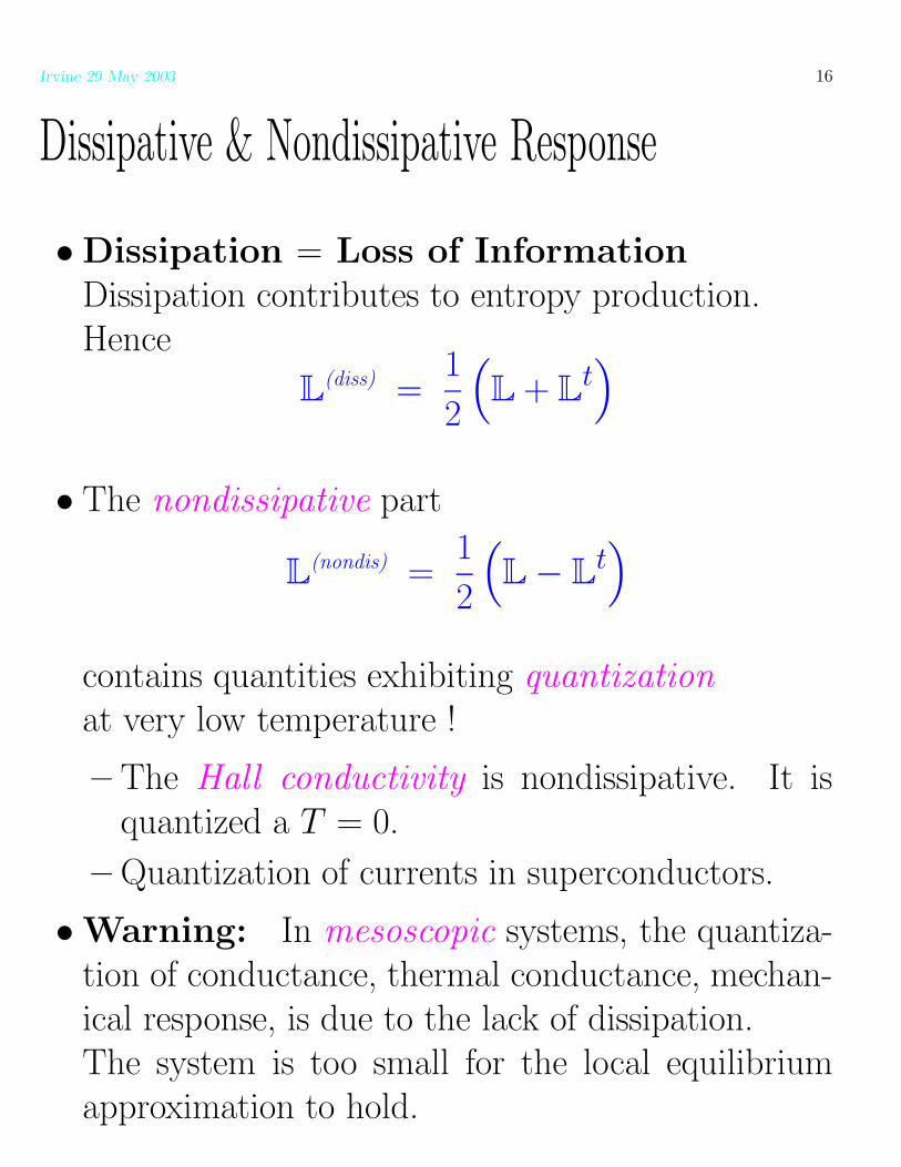
Dissipative & Nondissipative Response

• Dissipation = Loss of InformationDissipation contributes to entropy production.Hence

L(diss) =

1

2

(

L + Lt)

• The nondissipative part

L(nondis) =

1

2

(

L − Lt)

contains quantities exhibiting quantizationat very low temperature !

– The Hall conductivity is nondissipative. It isquantized a T = 0.

– Quantization of currents in superconductors.

• Warning: In mesoscopic systems, the quantiza-tion of conductance, thermal conductance, mechan-ical response, is due to the lack of dissipation.The system is too small for the local equilibriumapproximation to hold.


III - Kubo’s Formula


Mesoscopic Quantum Evolution

• Observable algebra A = AS ⊗AE

(S = system, E = environment).

• Quantum evolution ηt ∈ Aut(A),t ∈ R 7→ ηt(B) ∈ A continuous ∀B ∈ A.

• Initial state ρ ⊗ ρE

• System evolution

ρ(Φt(A)) = ρt(A) = ρ ⊗ ρE (ηt(A ⊗ 1))

Φt : AS 7→ AS is completely positive,Φt(1) = 1 and t 7→ Φt(A) ∈ AS is continuous.

• Markov approximation: for δt mesoscopic

Φt+δt ≈ Φt ◦ Φδt ≈ Φδt ◦ Φt

ThenδΦt

δt= L ◦ Φt = Φt ◦ L

L is the Linbladian.

• Dual evolution Φ†t(ρ) = ρ ◦ Φt giving rise to L

†.


Theorem 1 (Linblad ’76) If AS = B(H) and ifΦt is pointwise norm continuous, there is a boundedselfadjoint operator H on H and a countable familyof operators Li such that

L(A) = ı[H,A] +∑

i

(

L†iALi −

1

2{L

†iLi, A}

)

The first term of L is the coherent part and corre-sponds to a usual Hamiltonian evolution.The second one, denoted by D(A) is the dissipativepart and produces damping.

• Stationary states correspond to solutions ofL†ρ = 0.

• Equilibrium states are stationary states with max-imum entropy.They are equivalent to KMS states with respect tothe thermal dynamics which is generated by

Hth = H +

K∑

α=2

FαXα


Derivation of Greene-Kubo Formulæ

• In many cases there is a position operator acting onthe Hilbert space of states and given by a commutingfamily ~R = (R1, · · · , Rd) of selfadjoint operators.They describe the position of particles in the systemS.

• ~R generates a d-parameter group of automorphisms~k ∈ R

d 7→ eı~k·~RAe−ı~k·~R of the C∗-algebra AS.Thus ~∇ = ı[~R, · ] defines a ∗-derivation of AS.

• The mesoscopic velocity of the particles is given by

~V = L(~R) = ~∇H + D(~R)

The first part corresponds to the coherent velocitythe other to the dissipative one.

• The current associated with Xα is given by

~Jα =1

2{~V , Xα} = ~J

(coh)α + ~J

(diss)α


• At time t = 0, S is at equilibrium

⇒ ρS = ρeq. L†ρeq. = 0

• At t > 0, forces are switched on

E = (~E1, · · · , ~EK) with ~Eα = ~∇(Fα/T )

so that

LE = L +∑

α,j

EjαL

jα + O(E2)

• Hence the current becomes

JE ,i

α = J iα +

∑

α′,j

Ejα′{L

jα′(R

i), Xα} + O(E2)

• Then, if the forces are constant in time

~jα = limt↑∞

∫ t

0

ds

tρeq.

(

esLE ~J Eα

)

= limε↓0

∫ ∞

0εdt e−tερeq.

(

etLE ~J Eα

)

= limε↓0

ρeq.

(

ε

ε − LE

~J Eα

)

• Since L†ρeq. = 0, ρeq.

(

εε−L

~Jα

)

= 0


• Thus

~jα = limε↓0

ρeq.

(

ε

ε − LE

~J Eα −

ε

ε − L

~Jα

)

= limε↓0

ρeq.

(

ε

ε − L

∑

α′

~Eα′ · ~Lα′1

ε − LE

~Jα

)

+ limε↓0

ρeq.

(

ε

ε − L

∑

α′

E jα′ · {L

jα′(~R), Xα}

)

+ O(E2)

• Since ρeq. ◦ L = 0 this gives

jiα = −

∑

α′,j

E jα′ ρeq.

(

Ljα′

1

LJ i

α

)

+ρeq.

(

{Ljα′(R

i), Xα})

+ O(E2)

• Hence the Onsager cœfficients are

Li,jα,α′ = −ρeq.

(

Ljα′

1

LJ i

α + {Ljα′(R

i), Xα}

)


Validity of Greene-Kubo Formulæ

The previous derivation is formal. Various conditionsmust be assumed.

• The explicit expressions for L and the ~Lα′’s aremodel dependent.

• It is necessary to prove that LE(~R) ∈ AS.

• The inverse of L is not a priori well defined.

However, the dissipative part D is usually responsiblefor the existence of the inverse. This is because

Spec(ı[H, ·]) ⊂ ıR

while D gives a non zero real part to eigenvalues.In the Relaxation Time Approximation,

D(A) = A/τ ⇒ Spec

(

ı[H, ·] +1

τ

)

⊂ ıR +1

τ

where τ is the relaxation time.


IV - Relaxation Time Approximation


Conclusion

1. Linear response theory requires taking dissipationinto account. Various limits take care of time orlength scales.These limits usually do not commute !

2. Dissipation is described through the local equilib-rium approximation (LEA), leading to entropy cre-ation by constant return to local equilibrium.

3. Thanks to the LEA, the currents becomes smoothfunctions of the affinities leading to the transportor Onsager cœfficients.

4. A quantum treatment of transport cœfficients mustbe provided for electrons in a solid.The Master equation describes the dynamics withinthe LEA.

5. The Master Equation leads to the Greene-Kubo for-mula for Onsager cœfficients.

irvine 29 may 2003 linear response theory & kubo’s formula...

Documents