random matrix theory -...
TRANSCRIPT

Anderson & RMT Caltech Feb, 17th 2003 1
Random Matrix Theoryand
the 2D Anderson Model
Jean BELLISSARD1 2
Georgia Institute of Technology&
Institut Universitaire de France
Collaboration:
J. Magnen, V. Rivasseau, (Ecole Polytechnique, Palaiseau, France)
1Georgia Institute of Technology, School of Math & Physics, Atlanta, GA 30332-01602e-mail: [email protected]

Anderson & RMT Caltech Feb, 17th 2003 2
References:
This work
[1] J. Bellissard, J. Magnen, V. Rivasseau, Supersymmetric Analysis of a
Simplified Two Dimensional Anderson Model at Small Disorder,
cond-mat/0210524,
to be published in Markov Processes and Related Fields (2003).
[2] J. Bellissard, Coherent and dissipative transport in aperiodic solids, Pub-lished in Dynamics of Dissipation P. Garbaczewski, R. Olkiewicz (Eds.), LectureNotes in Physics, 597, Springer (2002), pp. 413-486.
Motivated by
[3] M. Disertori, H. Pinson, T. Spencer, Density of states for Random BandMatrix, math-ph/0111047, Commun. Math. Phys., 232, (2002), 83-124.

Anderson & RMT Caltech Feb, 17th 2003 3
The Anderson Model:
For H = `2(ZD)
Hω ψ (x) =∑
y;|x−y|=1
ψ(y) + V (x)ψ(x)
where ω = V (x)x∈ZD ∈ Ω is a family of i. i. d.’swith
〈V (x)〉 = 0 〈V (x)2〉 = W 2
The Anderson et al. conjecture:
1.D ≤ 2 pure point spectrum, with finite localizationlength for W > 0.
2.D ≥ 3 there is a region of the phase space (E,W )in which the spectrum is absolutely continuous withpositive residual conductivity.
Anderson & RMT Caltech Feb, 17th 2003 4
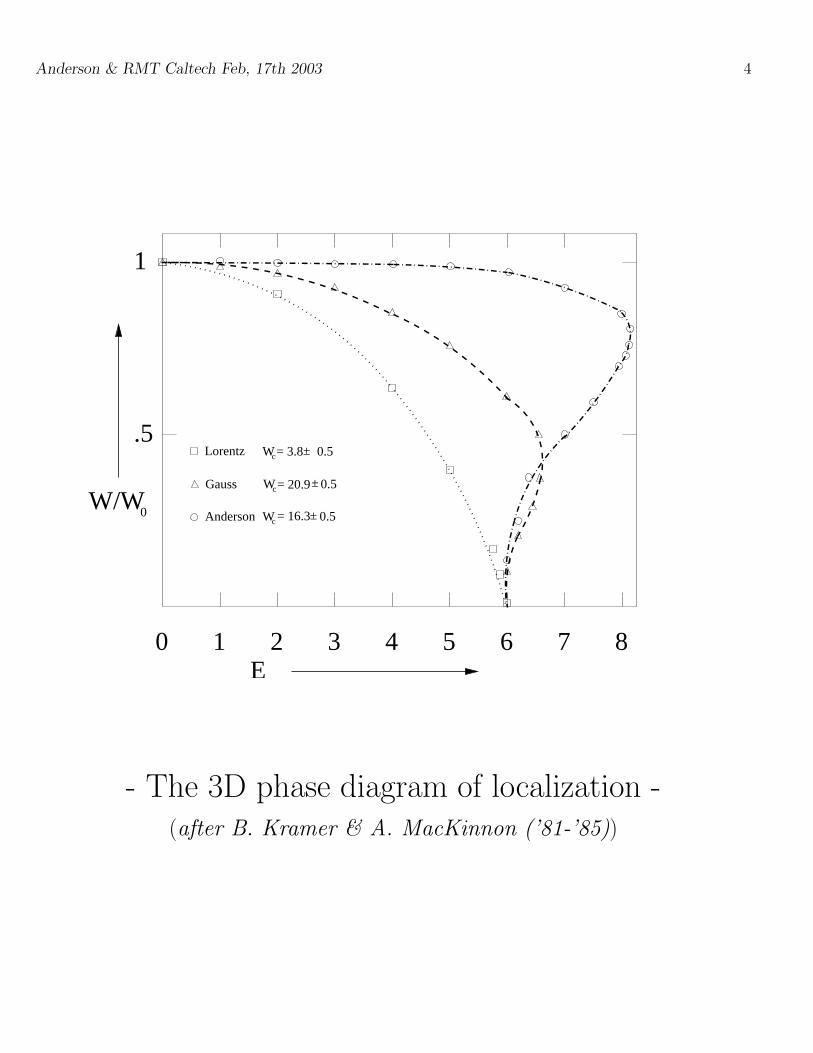
Wc +−Anderson 0.5= 16.3
+−Wc 0.5Lorentz = 3.8
+−Wc= 20.9 0.5Gauss
1 2 3 4 5 6 7 8
.5
1
0
W/W0
E
- The 3D phase diagram of localization -(after B. Kramer & A. MacKinnon (’81-’85))

Anderson & RMT Caltech Feb, 17th 2003 5
Results:
1. Anderson (1958): localization. Gang of 4 (1979):Anderson’s transition for D ≥ 3.
2. Wegner (1979)P: the n-orbital model;Wegner & Schaeffer (1980): Goldstone’s boson.
3. Numerics: Pichard-Sarma (1981-84)Kramer & MacKinnon (1981-86).
4. Rigorous 1D: Pastur-Molchanov (1978),Kunz-Souillard (1979).
5. Rigorous D ≥ 2: Frohlich-Spencer (1983),Frohlich-Spencer-Martinelli-Scoppola (1984),· · ·, Aizenman-Molchanov (1993).
6. Supersymmetry: Wegner, Efetov (1983).
7. Random Matrices: Altshuler-Shklovskii (1986),mesoscopic systems.
8. Universality: Quasicrystals Berger, Mayou et al. (1987-89)

Anderson & RMT Caltech Feb, 17th 2003 6
Noncommutative Calculus:
A covariant operator is a family A = Aω of opera-tors on H such that
1. ω 7→ Aω is measurable,
2. T (a)AωT (a)−1 = Ataω
(T (a) = translation by a ∈ ZD, t
aω = V (x− a)x∈ZD).
Trace per unit volume:
TP(A) =
∫
ΩP(dω)〈0|Aω|0〉 = lim
Λ↑ZD
1
|Λ|TrΛ(Aω)
P-almost surely (P = probability distribution of ω).
Derivatives:
(∂µA)ω = ı[Xµ , Aω] ~∇ = (∂1, · · · , ∂D)
X = (X1, · · · ,XD) position operator.

Anderson & RMT Caltech Feb, 17th 2003 7
IDS (Shubin’s formula):
IDS = Integrated Density of States
N (E) = limΛ↑ZD
1
|Λ|#eigen. Hω Λ≤ E
= TP(χ(H ≤ E)) a.e. ω
Current-Current correlation:
Current operator: ~J = e2/~ ~∇H .
TP(f (H) ∂νH g(H) ∂ν′H)
=
∫
R×R
mν,ν′(dE, dE′) f (E) g(E′)

Anderson & RMT Caltech Feb, 17th 2003 8
Transport:
Diffusion exponent:
(L∆(t))2 =
∫ +t
−t
ds
2t
∫
XdPtr(ω)
· · · 〈0|Πω,∆ | ~Xω(s) − ~X|2 Πω,∆|0〉
t↑∞∼ t2β2(∆) .
where Πω,∆ = χ(Hω ∈ ∆)
Equivalently (J. B. & H. Schulz-Baldes (‘98)), if
m(dE, dE′) =
D∑
ν=1
mν,ν(dE, dE′)
then
m(E,E′ ∈ ∆ × R ; |E − E′| ≤ εε↓0∼ ε2(1−β2(∆)) .

Anderson & RMT Caltech Feb, 17th 2003 9
Kubo’s formula:
In the Relaxation Time Approximation
σν,ν′ =e2
~
∫
R2mν,ν′(dE, dE
′)
· · ·fT,µ(E) − fT,µ(E′)
E′ − E
1
~/τcoll − ı(E′ − E),
T = temperature,µ = chemical potentialτcoll = average collision timekB = Boltzmann constant
fT,µ(E) =1
1 + e(E−µ)/kBT
Fermi level:
N (EF) = nelwhere nel is the charge carrier density.

Anderson & RMT Caltech Feb, 17th 2003 10
Theorem 1 If mν,ν′ = ρ(2)ν,ν′
dEdE′ with ρ(2)ν,ν′
(E,E′)
continuous near E = E′ = EF then, for any Borelset ∆ ⊂ R small enough containing EF
1. β2(∆) = 1/2
2. The diffusion constant D(∆) = limt↑∞L∆(t)2/tis finite and
D(∆) = π
∫
∆
dE∑
ν
ρ(2)ν,ν(E,E)
3. The DC conductivity at zero temperature is finiteand given by
σν,ν =πe2
~ρ
(2)ν,ν(EF , EF)

Anderson & RMT Caltech Feb, 17th 2003 11
Universality:
1. Other systems like quasicrystals exhibit diffusionexponents smaller than 1/2
2. At low temperature quasicrystals show a weak lo-calization regime as for the Anderson model (Mayou
et al. ‘98) suggesting β2 = 1/2.
3. Numerics show a Wigner-Dyson spectral statistics(Schreiber et al. ‘99) for the octagonal tiling.
How can these observations be reconciled ?Spectral statistics requires finite size sample. For asample of size L,Heisenberg’ time: it takes a time tH = O(LD) to seethe discretization of the spectrum.Thouless time: it takes a time tTh = O(L1/β2) forthe wave packet to reach the boundary.If tTh tH the wave packet feels only the finite size.
β2 > 1/D ⇒ weak localization

Anderson & RMT Caltech Feb, 17th 2003 12
Voiculescu’s Free Calculus:
Let A be unital algebra A.
1. A distribution is a linear map φ : A 7→ C such thatφ(1) = 1,
2. A random variable is an elementX of A. Its distri-bution is the map φX : p ∈ C[X ] 7→ φ(p(X)) ∈ C.
3.X1, · · · , Xn are free if for any (i1, · · · , il) ∈ [1, n]l
such that ik 6= ik+1 and any polynomials p1, · · · , pl
φ(pk(Xik)) = 0 ∀k ⇒ φ(
p1(Xi1) · · · pl(Xil))
= 0
4. free convolution: if X,Y are free, φX+Y dependsonly upon φX and φY and is denoted φX φY .
5. R-transform: if GX(z) = φ((z −X)−1)
GX =1
z −RX GX(z)
Then X,Y free ⇒ RX+Y = RX +RY .
Anderson & RMT Caltech Feb, 17th 2003 13
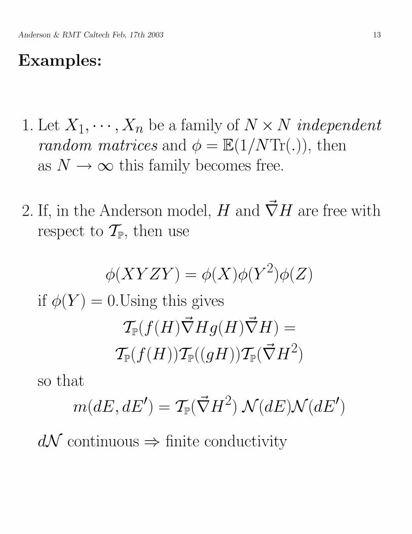
Examples:
1. Let X1, · · · , Xn be a family of N ×N independentrandom matrices and φ = E(1/NTr(.)), thenas N → ∞ this family becomes free.
2. If, in the Anderson model, H and ~∇H are free withrespect to TP, then use
φ(XY ZY ) = φ(X)φ(Y 2)φ(Z)
if φ(Y ) = 0.Using this gives
TP(f (H)~∇Hg(H)~∇H) =
TP(f (H))TP((gH))TP(~∇H2)
so that
m(dE, dE′) = TP(~∇H2) N (dE)N (dE′)
dN continuous ⇒ finite conductivity

Anderson & RMT Caltech Feb, 17th 2003 14
Wegner’s n-orbital Model:
Hω ψ (x) =∑
y;|x−y|=1
ψ(y) + V (x)ψ(x)
where ω = V (x)x∈ZD is a family of identically dis-tributed random n× n matrices with
〈V (x)〉 = 0 〈(V (x))2i,j〉 =W 2
n
Theorem 2 (i) In the limit n → ∞ the V (x)’s be-come free variables.(ii) In the limit n → ∞ the density of states dNand the current-current correlation of the Wegnermodel are continuous.
(Wegner ‘81)(Pastur-Khorunzhy ’93)(Neu-Speicher ’94)

Anderson & RMT Caltech Feb, 17th 2003 15
The DPS model:
H = (Hij) is a random gaussian matrix with zero av-erage and covariance
〈HijHkl〉 = δijδklJij
with
Jij =
(
1
−W 2∆ + 1
)
ij
where i, j vary in Λ ∩ Z3, Λ a set of cubes of size W
and W > 0 large but fixed. ∆ is the discrete Laplacianwith periodic b.c..
The DOS is defined by
ρΛ(E) =1
πlimε↓0
=〈
(
1
E + ıε−H
)
00〉
This model should behave like the 3D Anderson one.
Anderson & RMT Caltech Feb, 17th 2003 16
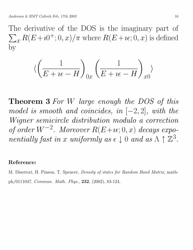
The derivative of the DOS is the imaginary part of∑
xR(E+ ı0+; 0, x)/π where R(E+ ıε; 0, x) is definedby
〈
(
1
E + ıε−H
)
0x
(
1
E + ıε−H
)
x0〉
Theorem 3 For W large enough the DOS of thismodel is smooth and coincides, in [−2, 2], with theWigner semicircle distribution modulo a correctionof order W−2. Moreover R(E+ıε; 0, x) decays expo-nentially fast in x uniformly as ε ↓ 0 and as Λ ↑ Z3.
Reference:
M. Disertori, H. Pinson, T. Spencer, Density of states for Random Band Matrix, math-
ph/0111047, Commun. Math. Phys., 232, (2002), 83-124.

Anderson & RMT Caltech Feb, 17th 2003 17
RMT & Anderson:Anderson’s model at weak coupling:(Poirot, Magnen, Rivasseau ’98):
1. The unperturbed Hamiltonian is the discrete Lapla-cian H0. Set χW = χ(|H0 − EF | ≤ c ·W 2)).
2. The part of the Hamiltonian with energies awayfrom EF by O(W 2) can be treated as a perturba-tion. Let them χW = χ(|H0 − EF | ≤ O(W 2)) andHeff = χWHχW .
3. Divide ZD into boxes of size O(W−2). In each such
box Λ, let VΛ be the restriction of Heff to Λ.
4. The VΛ’s play a role similar to the potential in theWegner n-orbital model with n = O(W−2). Theconnecting operators between boxes play the role ofthe discrete Laplacian.
5. For D = 2 and gaussian potential, the VΛ’s aregaussian random matrices of the type GOE with anextra discrete symmetry: flip matrices
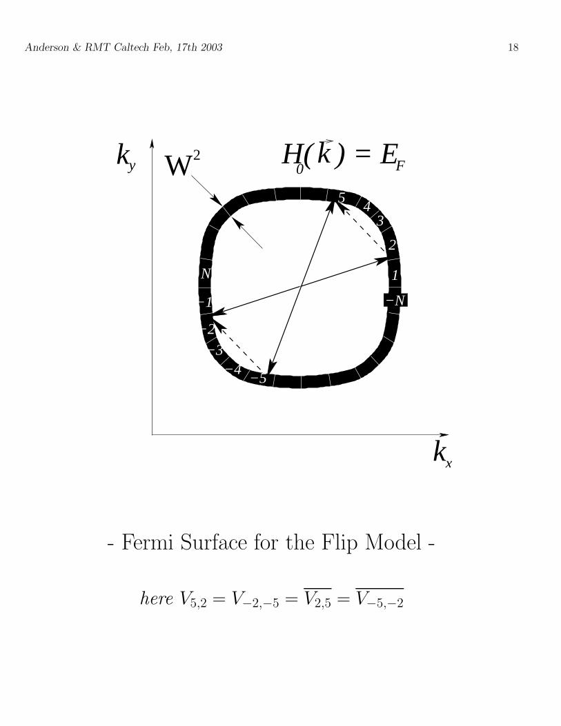
Anderson & RMT Caltech Feb, 17th 2003 18
kx
2Wyk0
H( ) = Ek F
1
2
34
5
N
−1
−2
−3−4
−5
−N
- Fermi Surface for the Flip Model -
here V5,2 = V−2,−5 = V2,5 = V−5,−2

Anderson & RMT Caltech Feb, 17th 2003 19
The Flip Matrix model for D = 2(JB, Magnen, Rivasseau ’02):
1. Since Λ is a finite box the quasimomentum space isdiscrete. The thicken Fermi surface defined by χW
contains only n = 2N = O(W−2) quasimomentadenotes by α, β ∈ 1, · · · , N ∪ −N, · · · ,−1
2. VΛ is a 2N×2N selfadjoint gaussian random matrix,indexed by quasimomenta
Vα,β = Vβ,α
3. Momentum conservation leads to
Vα,β = V−β,−α Vα,α = V0
4. Modulo these constraints the matrix elements areindependent and
〈Vα,β〉 = 0 〈|Vα,β|2〉 = W 2 = O(1/2N )
5. Main result: The DOS od the flip model is asemicircular distribution.

Anderson & RMT Caltech Feb, 17th 2003 20
About the Proof:
1. Using supersymmetry the DOS can be written as
dN
dE= lim
=mE↓0
1
π
∫
S++αS+α e
L DΨ†DΨ
where Ψ±α = (S±α, χ±α) is a superfield
L is a sum of quartic terms of the form
Ψ†±αΨ±βΨ
†±βΨ±α
2. Using commutation rules it can be written as a sumof terms of the form
Ψ†±αΨ±αΨ
†±βΨ±β
separating the α’s from the β’s.
3. Using a gaussian integral
eL =
∫
DR eıW∑
αΨ†αRΨα
where R varies in a set of 4 × 4 supermatrices.

Anderson & RMT Caltech Feb, 17th 2003 21
4. The gaussian integral can be performed and givesrise to a 5-dimensional integral of the form
∫
R5d5x (F (x))N
Since 1 N = O(W−2), this can be analyzedthrough a saddle point method.
5. Among the 4 saddle points only one contributes inthe limit N → ∞, giving rise to a semi-circle dis-tribution.
Anderson & RMT Caltech Feb, 17th 2003 22
Open Problems:
1. ForD ≥ 3, the previous model has a bigger degener-acy. A power counting of Feynmann graphs for theSUSY theory shows that the dominant contributioncomes from a flip matrix similar to the D = 2 case:Prove it.
2. The limit W ↓ 0 looks similar to a Wegner modelin any dimension: Prove it.
3. The limit W ↓ 0 cannot provide a good approxi-mation of the weak coupling case, since localizationis expected. In term of the SUSY field, this comes
a Goldstone mode which gets a mass e−O(W−2):Prove that for D ≥ 3 the Goldstone mode re-mains massless and that the limit W ↓ 0 gives agood approximation to the low coupling regime.