Final Report:

INVESTIGATION OF FAULT-TO-FAULT PREDICTIONS AND RESULTS FROM UCERF-3

PI: Glenn Biasi

University of Nevada, Reno

SCEC Proposal #13134

Introduction The Uniform California Earthquake Rupture Forecast 3 (UCERF3; Field et al., 2013) improved on previous rupture forecast models (Field et al., 2009) by relaxing the assumption of segmentation on major faults and by allowing ruptures to jump from one fault to another. The rupture forecast is expressed in terms of the estimated rates of individual ruptures. Each rupture is unique and constructed of some number of fault subsections under plausibility rules (Milner et al., 2013). A “Grand Inversion” estimates the rates of each rupture using a Monte Carlo method to fit slip rate on each subsection, paleoseismic event rates, and regional seismicity constraints. To construct ruptures, the plausibility rules are applied only between adjacent pairs of subsections. No distinction is made between subsection pairs that barely pass versus pairs that are touching and highly aligned. For example, a rupture containing subsections separated by 4 km is considered just as likely to occur in the input to the Grand Inversion as a rupture with no steps or bends in it. Thus the UCERF3 solution has been developed without making use of geologic information about relative rupture probability that might be gleaned from rupture geometry. This project develops empirical estimates of relative rupture probability from geometry and compares them to UCERF3 solution rates. We find a very limited correspondence between UCERF3 rupture rates and predictions from rupture complexity. Empirical Rupture Probabilities from Geometric Complexity Two types of structures in ruptures contribute to empirical rupture complexity. The first type is based on separation distance between subsections. Kinematic and dynamic modeling both find that steps in a rupture hinder rupture propagation (e.g., Lozos et al., 2011; Oglesby, 2005, 2008). The second type of complexity comes from fault bends and changes in rake. At these transitions, momentum in fault rupture is reduced by the change direction and by an increase in effective friction. The relationships of both types of complexity to probability are described in Biasi et al. (2013); preliminary results were presented in Biasi (2013). We consider three distance-related types of probability estimates for separations between subsections within a rupture. All ruptures begin with unit probability of occurrence. The empirical predicted rate is reduced by some factor for each instance in a rupture where consecutive subsections are separated by some minimum distance. Applied to full ruptures, rupture probability Pr depends on separation distance between ruptures, d as: Equation 1. Pr = Πps,s+1(d)

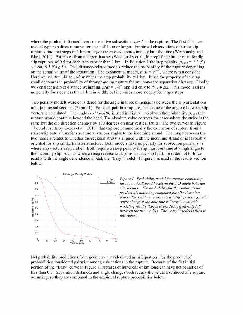
where the product is formed over consecutive subsections s,s+1 in the rupture. The first distance-related type penalizes ruptures for steps of 1 km or larger. Empirical observations of strike slip ruptures find that steps of 1 km or larger are crossed approximately half the time (Wesnousky and Biasi, 2011). Estimates from a larger data set (Wesnousky et al., in prep) find similar rates for dip slip ruptures. of 0.5 for each step greater than 1 km. In Equation 1 the step penalty, ps,s+1 = { 1 if d <1 km; 0.5 if d ≥ 1 }. Two distance-related models reduce the probability of the rupture depending on the actual value of the separation. The exponential model, p(d) = e-d/r0, where r0 is a constant. Here we use r0=1.44 so p(d) matches the step probability at 1 km. It has the property of causing small decreases in probability of through-going rupture for any non-zero separation distance. Finally we consider a direct distance weighting, p(d) = 1/dn, applied only to d>1.0 km. This model assigns no penalty for steps less than 1 km in width, but increases more steeply for larger steps.   Two penalty models were considered for the angle in three dimensions between the slip orientations of adjoining subsections (Figure 1). For each pair in a rupture, the cosine of the angle θ between slip vectors is calculated. The angle cos-1(abs(θ)) is used in Figure 1 to obtain the probability ps,s+1 that rupture would continue beyond the bend. The absolute value corrects for cases where the strike is the same but the dip direction changes by 180 degrees on near vertical faults. The two curves in Figure 1 bound results by Lozos et al. (2011) that explore parametrically the extension of rupture from a strike-slip onto a transfer structure at various angles to the incoming strand. The range between the two models relates to whether the regional stress is aligned with the incoming strand or is favorably oriented for slip on the transfer structure. Both models have no penalty for subsection pairs s, s+1 where slip vectors are parallel. Both require a steep penalty if slip must continue at a high angle to the incoming slip, such as when a steep reverse fault joins a strike slip fault. In order not to force results with the angle dependence model, the “Easy” model of Figure 1 is used in the results section below.

Figure 1. Probability model for rupture continuing through a fault bend based on the 3-D angle between slip vectors. The probability for the rupture is the product of continuing computed for all subsection pairs. The red line represents a “stiff” penalty for slip angle changes; the blue line is “easy”. Available modeling results (Lozos et al., 2011) generally fall between the two models. The “easy” model is used in this report.

Net probability predictions from geometry are calculated as in Equation 1 by the product of probabilities considered pairwise among subsections in the rupture. Because of the flat initial portion of the “Easy” curve in Figure 1, ruptures of hundreds of km long can have net penalties of less than 0.5. Separation distances and angle changes both reduce the actual likelihood of a rupture occurring, so they are combined in the empirical rupture probabilities below.

0 10 20 30 40 50 60 70 80 900

0.1

0.2

0.3

0.4

0.5

0.6

0.7

0.8

0.9

1Two Angle Penalty Models

Angle (degrees)

Prob

abilit

y of

Pas

sing

1: "Stiff"2: "Easy

Results Rupture probability from the Grand Inversion (GI) depends primarily on slip rates of subsections in the rupture. Because of that, a geometrically simple rupture with a high empirical geometric probability could have a high or low rate from the GI. Rates can be compared, however. In Figure 2, we compare GI rates to empirical rates using the set of UCERF3 FM3.1 ruptures 80-100 km long. The red line shows the normalized plot of log annual rates from the GI (x-axis “Rupture Rates”) for the full set. Because it is a full set, it necessarily includes ruptures on both high and low slip rate faults. We then find the ruptures with log-empirical probabilities of -1.2 to -0.8 – that is, ruptures judged a priori from their complexity to be an order of magnitude less likely than straight, simply connected ruptures. The GI probabilities for the complex rupture subsets are plotted as new

distributions, one each for angle+exp(d/ro), angle+step penalty, and angle+(1/d2) empirical probability models. If the GI reduced probabilities on complex ruptures by an amount similar to the empirical prediction, then the three curves would be offset to the left by an order of magnitude. As it is, there is no penalty in the GI for rupture complexity. Figure 2. GI probabilities for ruptures 80-100 km long. Red is all from FM3.1 in this set. Other curves are the GI probabilities for the fraction considered complex ruptures by three empirical models of complexity. The GI does not penalize ruptures in the subset for their complexity.

Figure 3. GI probabilities for all ruptures 80-100 km long and for subsets judged two orders of magnitude more improbable because of their complexity. At a log-empirical probability of -2 ruptures are extremely complex, at the level of, for example, three steps greater than 1 km plus two slip direction changes of 45 degrees. Figure 3 shows GI probabilities for this set are lower than the full set, although by 1 order of magnitude instead of the predicted 2. Some of the observed offset could be because of bias in the sample. Extremely complex ruptures are generally concentrated on low slip rate faults.

A normalization by slip rate (future work!) could help tease out the slip rate contribution. Figures 4 and 5 are plotted to investigate correlations between rupture complexity and GI rate estimates. Points are GI inversion results for individual ruptures. Only 1 in 20 is plotted to reduce the amount of overprinting. The vertical axes are two empirical complexity measures, one penalizing any separation distance by exp(d/r0), and the other applying and 0.5 penalty for steps greater than 1 km. Rupture subsets are color coded by length to look for systematic effects. In both Figures 4 and 5, if the GI reduced rupture probability (annual rate) by a similar amount to the empirical complexity estimates, the log-average rate summaries (heavy lines with “+” symbols) would descend to the left with a unity slope. A weak correlation is observed for ruptures of 60 to 140 km long, but at about half the predicted rate. Some degree of correlation is expected because the samples of complex ruptures are biased toward low slip rate faults. The poor correlation of GI

−10 −8 −6 −4 −20

0.1

0.2

0.3

0.4Length 80 < L <= 100

Rupture Rates

Nor

mal

ized

Fre

quen

cy

All Rupturesdot*exp(r/r0)dot*stepdot*(1/rn)

−10 −8 −6 −4 −20

0.1

0.2

0.3

0.4Length 80 < L <= 100

Rupture Rates

Nor

mal

ized

Fre

quen

cy

All Rupturesdot*exp(r/r0)dot*stepdot*(1/rn)

occurrence rate with the empirical rate from rupture geometry indicates that the GI is not materially penalizing ruptures for complexity. Ruptures with unlikely shapes are used at similar rates with simpler rupture topologies. In terms of the earthquake rate forecast as a whole, at some level, improbable and complex ruptures are absorbing slip rate and rupture frequency that a more complete model would concentrate on simpler ruptures. How important this effect is for hazard estimates remains to be seen.

Figure 4: Geometric complexity vs. UCERF3 solution rate for ruptures shorter than 200 km. Complexity measure = exp(r/r0)*dot-product of slip vector between subsections. Dots are individual rupture probabilities. Only 1 in 20 are plotted to keep them from overprinting. UCERF3 ruptures are binned by length (colors) and by rupture geometric complexity (lines with “+” symbols. A slope of 1 would mean that UCERF3 downweights complex

ruptures at a rate comparable to the geometric prediction. This is not observed except for ruptures shorter than ~140 km and complexity probability less than about a factor of 3 (exp(-0.5)).

Figure 5. Same as Figure 4, but geometric complexity estimated by a penalty of 0.5 for each separation between subsections that is greater than 1.0 km. UCERF3 probabilities follow the geometric prediction to ~-1.5 before becoming indifferent to additional complexity. −11 −10 −9 −8 −7 −6 −5 −4 −3 −2 −1

−5

−4.5

−4

−3.5

−3

−2.5

−2

−1.5

−1

−0.5

00.5nsteps*dot color steps: 20 km, wt: none

UCERF3 Solution Rate

Geo

met

ry P

redi

cted

Pro

babi

lity

L: 20−40L: 20−40L: 40−60L: 40−60L: 60−80L: 60−80L: 80−100L: 80−100L: 100−120L: 100−120L: 120−140L: 120−140L: 140−160L: 140−160L: 160−180L: 160−180L: 180−200L: 180−200

−11 −10 −9 −8 −7 −6 −5 −4 −3 −2 −1−5

−4.5

−4

−3.5

−3

−2.5

−2

−1.5

−1

−0.5

0Exp(r/r0)*dot color steps: 20 km, wt: none

UCERF3 Solution Rate

Geo

met

ry P

redi

cted

Pro

babi

lity

L: 20−40L: 20−40L: 40−60L: 40−60L: 60−80L: 60−80L: 80−100L: 80−100L: 100−120L: 100−120L: 120−140L: 120−140L: 140−160L: 140−160L: 160−180L: 160−180L: 180−200L: 180−200

Conclusions It is not surprising that the Grand Inversion is relatively insensitive to rupture complexity since no “complexity” data were provided as inputs. In mechanical modeling, complex geometry is a recognized and physically meaningful influence on the probability of through-going rupture. That role is recognized as well in observational geology. We find that well-posed empirical improbabilities (penalties) can be estimated a priori for ruptures on the UCERF3 fault geometry. Two applications of the empirical probability approach are suggested. First is as an additional constraint set for the Grand Inversion. If complex ruptures are less probable in the real world, an equation set can be constructed to implement it. Second, empirical probabilities can be used to trim the rupture set. At some level of complexity, rupture rates drop to the point of not being hazard significant. Rupture construction rules in UCERF3 were recognized as consciously inclusive, needing only to pass a “laugh test”. Empirical probabilities go a step further than just plausibility, testing rupture realism using rapid and physically meaningful criteria. References Biasi, G. (2013). Investigation of fault-to-fault predictions and results from UCERF3, Southern

California Earthquake Center Annual Meeting 2013 Proceedings Volume XXII, September 2013, poster 268.

Biasi, G. P., T. Parsons, R. J. Weldon II, and T. Dawson (2013). Fault-to-fault rupture probabilities, U.S.G.S Open-File Report 2013-1165, Uniform California Earthquake Rupture Forecast Version 3 (UCERF3) – The Time-Independent Model, Appendix J, 20 pp.

Field, E. H., G. P. Biasi, P. Bird, T. E. Dawson, K. R. Felzer, and 13 others (2013) Uniform California Earthquake Rupture Forecast Version 3 (UCERF3) – The Time-Independent Model, U.S.G.S Open-File Report 2013-1165, 115 pp.

Lozos, J.C., D. D. Oglesby, B. Duan, and S. G. Wesnousky (2011). The effects of double fault bends on rupture propagation: A geometrical parameter study, Bulletin of the Seismological Society of America, 101, 385-398.

Milner, K., M. T. Page, E. H. Field, T. Parsons, G. Biasi, and B. E. Shaw (2013). Defining the inversion rupture set via plausibility filters, U.S.G.S Open-File Report 2013-1165, Uniform California Earthquake Rupture Forecast Version 3 (UCERF3) – The Time-Independent Model, Appendix T, 14 pp.

Oglesby, D. D. (2005). The dynamics of strike-slip step-overs with linking dip-slip faults, Bulletin of the Seismological Society of America, 95, 1604-1622.

Oglesby, D. (2008). Rupture termination and jump on parallel offset faults, Bulletin of the Seismological Society of America, 98, 440-447.  

Wesnousky, S.G., and Biasi, G.P., 2011, The length to which an earthquake will go to rupture: Bulletin of the Seismological Society of America, 101, 1948-1950.