67

http://journals.tubitak.gov.tr/earth/

Turkish Journal of Earth Sciences Turkish J Earth Sci(2014) 23: 67-79© TÜBİTAKdoi:10.3906/yer-1306-5

Investigation of fault-related small-scale fluid flow in geothermal fields by numerical modeling

Doğa DÜŞÜNÜR DOĞAN*Department of Geophysical Engineering, Faculty of Mines, Istanbul Technical University, İstanbul, Turkey

* Correspondence: dusunur@itu.edu.tr

1. IntroductionHydrothermal fluid circulation is a very dominant process for exchanging the heat between different geological units within the earth. It is well known that hydrothermal fluid circulation is an extremely efficient mechanism for the heat transfer in both the submarine environment and the continental environment (Williams and Von Herzen, 1974; Sclater et al., 1980; Stein and Stein, 1994; Rabinowicz et al., 1998, 1999; Yang et al., 1998; Simms and Garven, 2004). Fluid flow is mostly driven by the natural thermal gradient or local heat sources for the continental environment. In turn, this thermally driven convective circulation can strongly affect the subsurface temperature field (Yang et al., 1998; Simms and Garven, 2004). This is the case particularly for the geothermal fields where natural thermal convection arises from unstable variation of fluid density due to uneven temperature distribution.

Due to the complexity of the present problem of finding temperature distributions within these geothermal areas, multidisciplinary approaches are usually required for the solution. Among them, the numerical technique is one of the most widely used for the solution; numerical computation of fluid flow involves solution of the coupled time dependent mass, energy conservation, and momentum equations subjected to the temperature and fluid flow boundary conditions (e.g., Fehn and Cathles, 1979; Fehn et al., 1983; Fisher et al., 1990; Lowel et al., 1995). A number of studies with various numerical

techniques were conducted to characterize the convection in a porous layer heated from below (e.g., Elder, 1967; Caltagirone, 1975; Baytas and Pop, 1999; Baytaş, 2000; Bilgen and Mbaye, 2001; Saleh et al., 2011). Elder (1967) studied free convection in a porous medium uniformly heated from below by the finite difference method. The results indicated the strong dependency of the solution on Rayleigh numbers. Kimura et al. (1986) developed a technique for high Rayleigh numbers to accurately simulate the convection with the pseudospectral method. Baytaş (2000) investigated the natural convection problem for a tilted rectangular cavity by using the finite difference control volume and alternating direction implicit (ADI) method.

Hydrothermal convection has also been a topic of many numerical studies in earth science (Lopez and Smith, 1995; Yang et al., 1998; Simms and Garven, 2004). Many authors have pointed out that existence of fractures within geothermal areas can play an important role in shaping the fluid flow pattern and smoothing the progress of fluid flow (Lopez and Smith, 1996; Yang et al., 1998; Simms and Garven, 2004). Free convection in a fault zone was first investigated by Murphy (1979). He modeled the fault by a vertical porous slot with a 2D high permeability field enclosed by impermeable but thermally conductive walls. These models indicate that the strength of the convective flow is proportional to the Rayleigh number. Convection cells that depend on the physical properties of the porous

Abstract: In this paper, hydrothermal circulations and temperature distributions in geothermal areas with fault zones are investigated. It is shown that existence of the fault zones influences both the fluid circulation patterns and velocities. Reciprocal influence of the local fluid circulations and the temperature distribution is demonstrated. A 2-dimensional square porous layer is used for modeling the geothermal field. Faults are modeled as vertical porous layers. It is assumed that faults are located inside the geothermal field and have a higher permeability than the field itself. Anisotropic and isotropic models are used to simulate the permeability structure of the faults. Several parametric studies, such as the different numbers, sizes, and locations of the faults within a geothermal field, are conducted. It is demonstrated that fluid flow pattern and temperature distribution are strongly linked to these parameters.

Key words: Thermal structure, fault, convection, permeability, modeling, stream function, geothermal

Received: 11.06.2013 Accepted: 11.10.2013 Published Online: 01.01.2014 Printed: 15.01.2014

Research Article

68

DÜŞÜNÜR DOĞAN / Turkish J Earth Sci

medium and the boundary conditions are controlled by the critical Rayleigh number ( ), which is the value for an infinite flat-lying porous medium with fixed upper and lower boundary temperatures (Nield and Bejan, 1999). As the Rayleigh number increases, the convective circulation pattern shifts progressively from a stable state to an unstable state with more complicated spatial and temporal behavior (Nield and Bejan, 1999). Numerical simulations indicate that the presence of faults alters the thermal convective flow pattern by constraining the size and location of convective cells (e.g., Lopez and Smith, 1995; Yang et al., 1998; Simms and Garven, 2004; Yang et al., 2004). Even fractures with apertures in the order of a few millimeters can convey significant flow rates of hot water from an order of depths of a kilometer (Lowell, 1975). Furthermore, Bixler and Carrigan (1986) presented numerical data that indicate that size and distribution of a fracture can significantly increase the heat transfer rate, which eventually leads to enhanced convection.

Furthermore, faults can induce convection in neighboring units even though the thermal conditions are not favorable for the convective flow. This is due to the fact that intrinsic permeability of the fault zone may force the Rayleigh number to exceed its critical threshold value locally.

Even though hydraulic properties of faults and fractures depend upon the geological setting, the state of stress, and the temporal evolution of the fault zone (Smith et al., 1991; Lopez and Smith, 1996), they can be identified by their high permeability compared to that of the neighboring geological units.

The objective of this study is to simulate the evolution of the fault-related small-scale circulation pattern by numerical modeling. The finite difference control volume (Patankar, 1980) and ADI methods are used to obtain the spatial changes of hydrothermal circulation under the effects of faulting. In the thermal modeling, effects of the depth, the thickness, and the number of the faulted zones in the fluid flow pattern are investigated. Isotropic and anisotropic models are used to represent the permeability structure of the fault zones. Several numerical simulations are conducted to reveal the nature and the evolution of the fault-related small-scale convection pattern in the densely faulted hot-water type of geothermal fields.

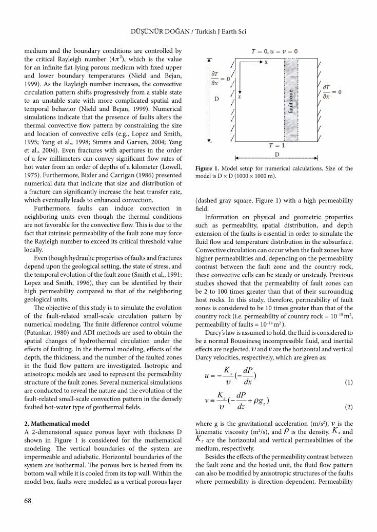
2. Mathematical modelA 2-dimensional square porous layer with thickness D shown in Figure 1 is considered for the mathematical modeling. The vertical boundaries of the system are impermeable and adiabatic. Horizontal boundaries of the system are isothermal. The porous box is heated from its bottom wall while it is cooled from its top wall. Within the model box, faults were modeled as a vertical porous layer

(dashed gray square, Figure 1) with a high permeability field.

Information on physical and geometric properties such as permeability, spatial distribution, and depth extension of the faults is essential in order to simulate the fluid flow and temperature distribution in the subsurface. Convective circulation can occur when the fault zones have higher permeabilities and, depending on the permeability contrast between the fault zone and the country rock, these convective cells can be steady or unsteady. Previous studies showed that the permeability of fault zones can be 2 to 100 times greater than that of their surrounding host rocks. In this study, therefore, permeability of fault zones is considered to be 10 times greater than that of the country rock (i.e. permeability of country rock = 10–15 m2, permeability of faults = 10–14 m2 ).

Darcy’s law is assumed to hold, the fluid is considered to be a normal Boussinesq incompressible fluid, and inertial effects are neglected. and are the horizontal and vertical Darcy velocities, respectively, which are given as:

(1)

(2)

where g is the gravitational acceleration (m/s2), is the kinematic viscosity (m2/s), and is the density. and

are the horizontal and vertical permeabilities of the medium, respectively.

Besides the effects of the permeability contrast between the fault zone and the hosted unit, the fluid flow pattern can also be modified by anisotropic structures of the faults where permeability is direction-dependent. Permeability

D

D

z

x

faul

t zon

e

Figure 1. Model setup for numerical calculations. Size of the model is D × D (1000 × 1000 m).

69

DÜŞÜNÜR DOĞAN / Turkish J Earth Sci

of faults and fractures is generally quite complex in both time and space (Smith et al., 1990; Caine et al., 1999; Aydin, 2000). The small-scale variations in permeability within a fault can increase/decrease the bulk permeability by one order of magnitude. For example, the ratio of the maximum principal values to minimum principal values of permeabilities is taken as Kmax/Kmin = 5 by Durlofsky (1992) and Taylor et al. (1999), where Kmax and Kmin are the maximum and minimum principal values of permeability, respectively. Thus, in the numerical simulations both isotropic and anisotropic cases are considered and used to obtain the fluid flow pattern. For the saturated porous medium, nondimensional governing equations of stream function and temperature are given as (Holzbecher, 1998):

(3)

(4)

where is the Darcy number, is the Rayleigh number, and is the dimensionless time. and are the dimensionless horizontal and vertical components of the Darcy velocity, respectively, defined as:

(5)

where the nondimensional variables are given by:

(6)

here, is the effective thermal diffusivity of the porous medium (m2/s), is the coefficient of thermal expansion (K–1), is the permeability of the porous layer (m2), is the temperature differences between the hot temperature of bottom wall and cold temperature of the top wall (i. e.

), and is the modified Rayleigh number. In the numerical simulations, the kinematic viscosity

is taken as constant, and the density is supposed to decrease linearly with temperature as:

(7)

where and are the reference density and temperature, respectively.

In addition to the Rayleigh number, it is useful to introduce other global measures of convective vigor (Lennie et al., 1998; Cherkaoui and Wilcock, 1999). It is well known that the Nusselt number ( ) is used to determine the heat flux efficiency of the system. The local Nusselt number ( ), which provides a dimensionless measure of the heat flux across the porous medium, can be obtained from the temperature field as follows:

(8)

The average Nusselt number is also defined as:

(9)

and the time-averaged Nusselt number is:

(10)

The initial and boundary conditions for governing Eqs. (3) and (4) are:when for whole space:

(11)

when (12)

(13)

(14)

3. Numerical solution procedureCoupled momentum and energy Eqs. (3) and (4) are discretized on the n × n points in a square grid region shown in Figure 1 and solved numerically by using the finite difference control volume method of Patankar (1980) in the Fortran PowerStation 4.0 platform. The resulting algebraic equations are then solved by the ADI method. Convergency of the present model is tested by using 7 sets of uniform grids for the Nusselt numbers for the steady-state cases (Table 1). It is found that grid size of 52 × 52 provides the optimum results in terms of the numerical accuracy, stability, and computational time. As a benchmark study, the present model on a 52 × 52 grid scheme is compared to previous works in terms of Nusselt numbers and maximum values of stream functions at different Rayleigh numbers (Table 2). It is apparent that

70

DÜŞÜNÜR DOĞAN / Turkish J Earth Sci

the results of the present study agree well with those of Caltagirone (1975) and Bilgen and Mbaye (2001).

A dimensionless time step of 0.001 is taken for this investigation. The solution procedure from the initial state is iterated until a steady-state is reached by satisfying the following convergence criterion with respect to each variable (Baytaş, 1996; Baytaş, 1997):

(15)

where e is the prescribed error, which is taken as 10–5.

4. ResultsThree types of models are used in this study to demonstrate the effects of fault structures on the distribution of fluid flow and temperature within a geothermal field: 1) model without fault, 2) model with single anisotropic fault, and 3) model with multiple anisotropic faults. These models provide some basic knowledge of the fluid flow and related temperature distribution with regard to the spatial locations, thicknesses, depths and anisotropic characteristics of faults.

In all models, the model box shown in Figure 1 is used, as stated earlier. The top and the bottom temperatures are taken as 10 °C and 300 °C, respectively. The model box size of D = 1000 m is taken. Thermal diffusivity and the thermal conductivity of the fluid saturated medium are α = 6.9 × 10–7 and k = 2.3. W/m °C, respectively. The value

of the Rayleigh number depends on the size of the model and was calculated by using the boundary conditions and the permeability of faults and hosted unit for given fluid properties ( ).

In the first model, an unfaulted porous layer is considered. This model represents the reference state for the other models since it does not include any disturbing effect of faults on the fluid flow and temperature distribution. The fluid flow velocity vectors that form 4 main contrarotative circulation cells inside the box are shown in Figure 2a. Maximum horizontal and vertical fluid velocities are 4.4 × 10–8 m/s and 6.9 × 10–8 m/s, respectively. The associated temperature distribution, which is symmetrical with respect to the center line of the model, is given in Figure 2b.

In the second model, a single permeable anisotropic fault (i.e. Kz = 5Kx) with a constant thickness along the box depth is used to demonstrate the geometry of formed convection cells and their effects on temperature distribution. It will be shown that a single fault in the model is an efficient way to demonstrate the role of the high permeable zone in the vertical heat transfer. In turn, efficiency of heat transfer can constrain the locations of convection cells.

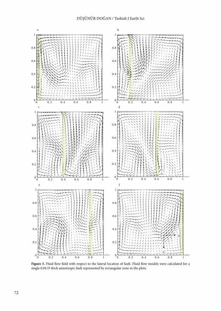
Thickness of a fault in the field can range from tens of meters to hundreds of meters. Therefore, the numerical simulations were performed for a wide range of thicknesses of 40, 60, 80, 100, 120, 140,160, and 200 m, but only the extreme cases of 40 m (0.04 D), 100 m (0.1 D), and 200 m (0.2 D) are presented in this paper. In addition to the varying fault thickness, varying fault depths of 250 m, 500 m, and 1000 m (rising from the bottom to the top of the model) were also modeled and the extreme case of 1000 m (1.0 D) is presented. Figure 3 displays the 2-dimensional fluid flow velocities when a single fault with a thickness of 0.04 D is located in different lateral locations at a time in the box system. In Figures 3a–3f, a relatively thin anisotropic single fault of 0.04 D is placed on the wall (Figure 3a) and then replaced very close to the left wall (Figure 3b).

Table 1. Accuracy test ( ).

Grid sizes

32 × 32 7.793642 × 42 7.857352 × 52 7.857072 × 72 7.8570102 × 102 7.8570

Table 2. Comparisons of solutions for various numerical experiments.

Present study Saleh et al., 2011 Bilgen and Mbaye, 2001 Caltagirone, 1975

50 1.451 2.108 1.454 2.116 1.443 2.092 1.45 2.112100 2.652 5.363 2.654 5.370 2.631 5.359 2.651 5.377150 3.336 7.372 3.336 7.379 - - - -200 3.830 8.935 3.830 8.941 3.784 8.931 3.813 8.942250 4.223 10.248 4.222 10.253 4.167 10.244 4.199 10.253300 4.551 11.397 4.459 11.400 4.487 11.394 4.523 11.405

71

DÜŞÜNÜR DOĞAN / Turkish J Earth Sci

In these cases, 4 main contrarotative circulation cells are created. It can be seen that the temperature distribution in the box system does not depend on the exact position of the fault when a single fault is placed near the left wall (Figures 4a and 4b). Figures in the second row (Figures 3c and 3d and Figures 4c and 4d) illustrate the fluid flow pattern and temperature distribution, respectively, when a single anisotropic fault is placed at about the midline region. Four main contrarotative circulation cells are created. Fluid flow velocities and temperature distribution inside the box are very different from those of previous cases where faults were close to the wall. Fluid flow and temperature distribution patterns for a single fault close to the right wall (Figures 4e and 4f) are very similar those of the single fault close to the left wall (Figures 4a and 4b), as expected. Maximum horizontal and vertical fluid velocities are 5.6 × 10–8 m/s and 7.4 × 10–8 m/s, respectively. Those velocities are slightly higher than those observed in the unfaulted model.

It is obvious that the existence and the location of a single fault strongly influence the fluid and thermal characteristics of the geothermal unit. In these models, the average Nusselt number is also lower (average Nu = 5.25) than in the other single fault models (average Nu = 6.12).

Figures 5a–5e and 6a–6e demonstrate the effects of the spatial location of the 0.2 D thick anisotropic fault on fluid flow and temperature, respectively. For a larger fault thickness, a greater effect of the fault on the convection system was observed. For this model, maximum horizontal and vertical fluid velocities are 7.1 × 10–8 m/s and 8.9 × 10–8 m/s, respectively (Figure 5). Overall average fluid velocities are higher than in the model presented in Figure 3. Furthermore, as the fault thickness increases, heat flux efficiency is also increasing, yielding higher Nusselt numbers. Thicker faults result in more visible differences in the fluid flow pattern and temperature contours, as well

(Figures 5 and 6). When the fault is located at the center of the system, 2 main fluid flow cells and 2 side cells are placed symmetrically at the side of the fault zone (Figure 5c). The size of the cells and their senses of rotation vary throughout the flow field.

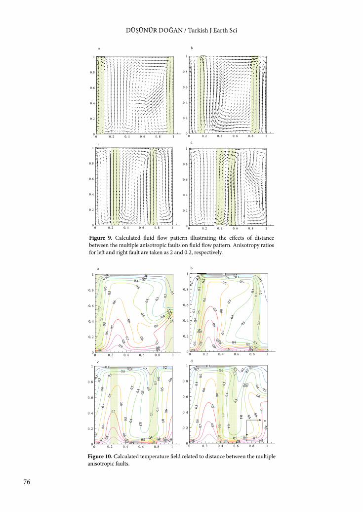
In the third model, the aim is to illustrate the effects of distance between the multiple faults on the fluid flow patterns and the temperature distributions. For simulation, 2 faults with a thickness of 0.1 D each were introduced to the model box, and the distance between 2 faults was decreased gradually from 0.9 D to 0.04 D, as shown Figures 7a–7d).

The vertical fractures inside the faults lead to less hydraulic resistance in the vertical direction. The vertical component dominates the transport phenomena inside the fault and in the vicinity of the fault. It can be seen from Figures 7a, 7b, and 7d that when the directions of the velocities are the same within both faults, the circulation patterns are symmetrical with respect to the vertical centerline, and they are antisymmetrical when the velocities are in the opposite direction, as in Figure 7c. Since the heat is mainly transported by fluid flow, in the box far from the faults, the horizontal and vertical components of the fluid flow are evenly accountable for the heat transfer. Figure 8 demonstrates the associated temperature field for this model.

Figures 9 and 10 show the same model, except that the faults have different permeability ratios. The permeability ratio of the left fault (Kz/Kx = 2) is kept the same, but the right fault is decreased by 10-fold (i.e. Kz/Kx = 0.2). Contrary to the previous case (Figures 7 and 8), no symmetry is seen in either velocity or temperature distribution in this case, as expected.

The influences of the anisotropic structure of the faults on the hydrothermal field are investigated by using various orders of the permeability ratio for a single centrally

0 0.2 0.4 0.6 0.8 10

0.2

0.4

0.6

0.8

1 0.10.1

0.2

0.2

0.2

0.3

0.3

0.3

0.3

0.3

0.4

0.4

0.4

0.4

0.4

0.4

0.4 0.5

0.5

0.5

0.5

0.5

0.5

0.50.5

0.5

0.6

0.60.6

0.60.6

0.6

0.6

0.6 0.7

0.70.7

0.7 0.8

0.80.8 0.90 0.2 0.4 0.6 0.8 10

0.2

0.4

0.6

0.8

1a b

x

z

Figure 2. Fluid flow (left) and temperature field (right) for model without faults. Contour interval for temperature field is 0.1.

72

DÜŞÜNÜR DOĞAN / Turkish J Earth Sci

0 0. 2 0. 4 0. 6 0. 8 10

0.2

0.4

0.6

0.8

1

0 0. 2 0. 4 0. 6 0. 8 10

0.2

0.4

0.6

0.8

1

0 0. 2 0. 4 0. 6 0. 8 10

0.2

0.4

0.6

0.8

1

0 0. 2 0. 4 0. 6 0. 8 10

0.2

0.4

0.6

0.8

1

0 0. 2 0. 4 0. 6 0. 8 10

0.2

0.4

0.6

0.8

1

0 0. 2 0. 4 0. 6 0. 8 10

0.2

0.4

0.6

0.8

1

x

z

a b

c d

e f

xx

Figure 3. Fluid flow field with respect to the lateral location of fault. Fluid flow models were calculated for a single 0.04 D thick anisotropic fault represented by rectangular zone in the plots.

73

DÜŞÜNÜR DOĞAN / Turkish J Earth Sci

0.10.1

0.20.2

0.2 0.3

0.30.3

0.3 0.4

0.4

0.4

0.4

0.4

0.5

0.5

0.5

0.5

0.6

0.6

0.6

0.6

0.7

0.7

0.7

0.80.8

0.8

0.90.9

0.9

0 0. 2 0. 4 0. 6 0. 8 10

0.2

0.4

0.6

0.8

1 0.10.10.2

0.20.2

0.2

0.3

0.30.3

0.3

0.4

0.4

0.4

0.40.4

0.5

0.5

0.5

0.50.50.5

0.6

0.6

0.6

0.6

0.6

0.6

0.6

0.7

0.7

0.7

0.7

0.80.8

0.8

0.90.9

0.90 0. 2 0. 4 0. 6 0. 8 10

0.2

0.4

0.6

0.8

1

0.10.1 0.2

0.2

0.2

0.3

0.3

0.3

0.3

0.4

0.4

0.4

0.4

0.4

0.5

0.5

0.5

0.50.5

0.5

0.5

0.6

0.60.6

0.6

0.6

0.6

0.6

0.7

0.7

0.7

0.70.7

0.8

0.8

0.80.90.9

0 0. 2 0. 4 0. 6 0. 8 10

0.2

0.4

0.6

0.8

1 0.10.1

0.2

0.2

0.2

0.3

0.30.3

0.3 0.4

0.40.4

0.4

0.4 0.5

0.5

0.5

0.5

0.5

0.5 0.6

0.6

0.6

0.6

0.70.7

0.7

0.7

0.80.80.8 0.90.90 0. 2 0. 4 0. 6 0. 8 10

0.2

0.4

0.6

0.8

1

0.10.1

0.1

0.2

0.2

0.2

0.3

0.3

0.3

0.3

0.4

0.4

0.4

0.4

0.4

0.5

0.5

0.5

0.5

0.5

0.5

0.6

0.6

0.6

0.6

0.7

0.7

0.7

0.7

0.8

0.80.8

0.8

0.90.90 0. 2 0. 4 0. 6 0. 8 10

0.2

0.4

0.6

0.8

1 0.10.1

0.2

0.20.2

0.3

0.30.3

0.3

0.40.4

0.4

0.4

0.5

0.5

0.5

0.5

0.6

0.60.6

0.6

0.7

0.70.7

0.7

0.80.8

0.8

0.90.90 0. 2 0. 4 0. 6 0. 8 10

0.2

0.4

0.6

0.8

1

a b

c

e

x

z

d

f

222222

00000.4444444.000.00555555

0

66666

0.0077777

000001

0000.00999999

11111

000.0055555

0.0088888

00.5555550.0.

0.0055

00000.0066666

00

0.00777777xxxxx

00000444444

0

0.777..

8888800088880.99999

Figure 4. Temperature distribution in the presence of single 0.04 D thick anisotropic fault. Contour interval for temperature is 0.1.

74

DÜŞÜNÜR DOĞAN / Turkish J Earth Sci

0 0.2 0.4 0.6 0.8 10

0.2

0.4

0.6

0.8

1

0 0.2 0.4 0.6 0.8 10

0.2

0.4

0.6

0.8

1

0 0.2 0.4 0.6 0.8 10

0.2

0.4

0.6

0.8

1

0 0.2 0.4 0.6 0.8 10

0.2

0.4

0.6

0.8

1

0 0.2 0.4 0.6 0.8 10

0.2

0.4

0.6

0.8

1

a b

x

z

d e

c

0.1

0.2

0.2

0.3

0.3

0.3

0.4

0.4

0.4

0.4

0.4

0.5

0.5

0.5

0.5

0.50.5

0.6

0.6

0.6

0.6

0.7

0.7

0.7

0.7 0.8

0.80.8 0.90.90 0.2 0.4 0.6 0.8 10

0.2

0.4

0.6

0.8

1 0.1

0.1

0.2

0.2

0.2

0.3

0.3

0.4

0.4

0.4

0.40.4

0.4

0.5

0.5

0.5

0.5

0.5

0.5

0.6

0.6

0.6

0.6

0.6

0.6

0.60.7

0.7

7

0.8

0.80

0.9

0.90 0.2 0.4 0.6 0.8 10

0.2

0.4

0.6

0.8

1 0.1.1 0.2

0.2

0.3

0.30.3

0.4

0.4

0.40.4

0.4

0.4

0.50.5

5

0.5

0.5

0.50.6

0.6

06

6

.

0.6

0.6

0.7

0.7

0.7

0.7

0.7

0.8

0.80.8

0.8

0.90.90 0.2 0.4 0.6 0.8 10

0.2

0.4

0.6

0.8

1

0.10.10.1 0.2

0.2

0.3

0.3

0.3

.

0.3

0.3

0.40.4

0.40.4

0.4

0.4

0.4 0.50.5

0.5

0.5

0.5

0.6

0.60.6

0.6

0.6

0.7

0.7

0.7

0.7

0.80.8

0.8

0.90.90 0.2 0.4 0.6 0.8 10

0.2

0.4

0.6

0.8

1

0.1

010.1

0.2

0.2

0.2

0.2

0.3

0.3

0.3

0.4

0.4

0.4

0.4

0.4

0.4

50.5

0.5

0.5

0.5

0.5

0.

0.6

0.6

0.6

0.6

0.7

0.7

0.7

0.80.80.8

090.90.90 0.2 0.4 0.6 0.8 10

0.2

0.4

0.6

0.8

1

a b

x

z

d e

c

00.00555555555 0000000.0088888888888 0000000.00999999999

00066600

0

7777

00

55555

0006666

6666

000007777700000

0000000

11111

00000.003333333333

0333.3000000000044400000

00

00000.001111111

000011

00000.00222222222222

00220

555555 000000008888800000000000000000099998888888888889

Figure 5. Fluid flow field with respect to the lateral location of fault. Fluid flow models were calculated for a single 0.2 D thick anisotropic fault.

Figure 6. Temperature distribution in the presence of a single 0.2 D thick anisotropic fault.

75

DÜŞÜNÜR DOĞAN / Turkish J Earth Sci

0 0. 2 0. 4 0. 6 0. 8 10

0.2

0.4

0.6

0.8

1

0 0. 2 0. 4 0. 6 0. 8 10

0.2

0.4

0.6

0.8

1

0 0. 2 0. 4 0. 6 0. 8 10

0.2

0.4

0.6

0.8

1

0 0. 2 0. 4 0. 6 0. 8 10

0.2

0.4

0.6

0.8

1

a b

x

z

dc

Figure 7. Calculated fluid flow pattern illustrating the effects of distance between the multiple anisotropic faults on fluid flow pattern. Anisotropy ratio for both faults is taken as 2 (Kz/Kx = 2).

0.1

0.2

0.20.2

0.2

0.3

0.3

0.30.3

0.3

0.3 0.4

0.4

0.4

0.

0.4

0.4

0.4

0.4

0.5

0.5

0.5

0.5

0.5

0.5

0.5

0.5

0.60.6

0.6

0.6

0.6

0.6

0.6

0

0.70.70.7

0.70.7

0.7

0.8

0.8

0.8

0.8

0.90.9

0.9

0 0. 2 0. 4 0. 6 0. 8 10

0. 2

0. 4

0. 6

0. 8

1

0.1

0.1

0.2

0.2

0.2

0.2

0.2

0.3

0.3

0.3

0.3

0.3

0.4

0.4

0.4

0.4

0.4

0.4

0.5

0.5

0.5

0.5

0.5

0.5

0.5

0.60.60.6

0.6 0.7

0.7

0.7 0.80.8 0.90.90 0. 2 0. 4 0. 6 0. 8 10

0. 2

0. 4

0. 6

0. 8

1

0.10.1

0.2

0.2

0.2 0.3

0.3

0.30.3

0.3

0.4

0.4

0.4

0.4

0.4

0.4

0.4

0.5

0.5

0.5

0.5

0.5

0.5

0.50.5

0.6

0.6

0.6

0.6

0.6

0.6

0.60.6

0.7

0.7

0.70.7

0.7 0.8 0.90.90.90 0. 2 0. 4 0. 6 0. 8 10

0. 2

0. 4

0. 6

0. 8

1 0.10.1 0.20.2

0.3

0.3

0.3

0.3

0.4

0.40.4

0.4

0.4

0.50.5

0.50.5

0.50.5

0.6

0.6

0.6

0.6

0.6

0.6 0.7

0.7

0.7

0.70.7

0.7

0.7

0.8

0.8

0.8

0.8

0.9

0.9

0.90 0. 2 0. 4 0. 6 0. 8 10

0. 2

0. 4

0. 6

0. 8

1

a b

x

z

dc

000.0022222

0.0033

0000000

000.00888888800000.00999999 .889

000.00222222

3333

33

0000333304444444444.40000.00555555005

000.0777777

00088888888.8000

00000.0099999999

0000022222

22

00000.00333333333

7777777 0000

00022222

0.0022

00000.003333333

00000.0088888

0000.0066666666

06.60

00077770000.0077777777

00000.00222222 0000022 033333

0000333 00044

0000000.0044444444400000.0066666

00000.0066666666

00007000.0077777 06.600

0000.007777770000888888

999

Figure 8. Calculated temperature field related to distance between the multiple anisotropic faults.

76

DÜŞÜNÜR DOĞAN / Turkish J Earth Sci

0 0. 2 0. 4 0. 6 0. 8 10

0. 2

0. 4

0. 6

0. 8

1

0 0. 2 0. 4 0. 6 0. 8 10

0. 2

0. 4

0. 6

0. 8

1

0 0. 2 0. 4 0. 6 0. 8 10

0. 2

0. 4

0. 6

0. 8

1

0 0. 2 0. 4 0. 6 0. 8 10

0. 2

0. 4

0. 6

0. 8

1

x

z

a b

dc

Figure 9. Calculated fluid flow pattern illustrating the effects of distance between the multiple anisotropic faults on fluid flow pattern. Anisotropy ratios for left and right fault are taken as 2 and 0.2, respectively.

0.1

0.10.1

0.2

0.20.2

0.3

0.30.3

0.3

0.4

0.4

0.4

0.4

0.4

0.50.5

0.50.5 0.6

0.6

0.6

0.6

0.6

0.7

0.7

0.7

0.8

0.8

0.8

0.8 0.90.9

0 0. 2 0. 4 0. 6 0. 8 10

0. 2

0. 4

0. 6

0. 8

1

0.1

0.1

0.1

0.2

0.2

0.2

0.3

0.3

0.3

0.3

0.3

0.4

0.4

0.4

0.4

0.0.4

0.5

0.50.5

0.5

0.50.5

0.6

0.60.6

0.6

0.60.6

0.7

0.70.7

0.7

0.80.8

0.8

0.8

0.9

0.9

090 0. 2 0. 4 0. 6 0. 8 10

0. 2

0. 4

0. 6

0. 8

1

0.10.1 0.2

0.2

0.2

0.2

0.30.3

0.3

0.3

0.3

0.3

0.4

0.4

0.4

0.4

0.4

0.4 0.5

0.5

0.5

0.50.5

0.5

0.5

0.5

0.60.6

6

0.60.6

0.6

0.6

0.70.7

0.7

0.7 0.80.8

0.8 0.90.90.90 0. 2 0. 4 0. 6 0. 8 10

0. 2

0. 4

0. 6

0. 8

1

0.1

0.1 0.20.20.2

0.3

0.3

0.3

0.3

0.3

0.40.4

0.4

0.4

0.4

0.4

0.4 0.5

0.5

0.5

0.5

0.50.5

0.6

0.6

0.6

0.60.6

0.6

0.6

0.7

0.7

0.7

0.7

0.7 0.8

.8

0.8

0.8 0.90.90.90 0. 2 0. 4 0. 6 0. 8 10

0. 2

0. 4

0. 6

0. 8

1

x

z

a b

dc

000

00000.003333000.0044444444

005

0.008888

0000.001

0.002222

00000.008888

00000.00000.555555..

00000.00666666000.0066666 00000..0000 0.0077777776666 7

000.88888880..

0.001

00000.002222222

0222.200

0000.003333333

0000.00333330.004444

00000.666666660..7777799999977779

0.00555555

0.0066666

00000.00777777

0022222222

00000.003333333000.003333333

000044400

000000.004444444

000.0055555

00000555

000.006666660000066666666

00000.0077777

0000000.00999999999

000.00222222

00000.003333

0000 2033333333333.300000004444

Figure 10. Calculated temperature field related to distance between the multiple anisotropic faults.

77

DÜŞÜNÜR DOĞAN / Turkish J Earth Sci

located fault (Figures 11 and 12). The permeability ratio of the vertical direction to the horizontal direction is assumed to vary from 0.1 to 10 (i.e. Kz/Kx = 0.1 to 10). It can be clearly seen that when the ratio of Kz/Kx increases, the magnitude of the horizontal components of the field velocities within the faults diminishes; however, that of the vertical components of field velocities increases as expected (Figure 11). Increase in the permeability ratio causes an increase in the magnitude of velocities, and the formation of new symmetrical vortex-type patterns in the geothermal field becomes apparent. The isotherms in the fault itself are flat when the permeability ratio is small; however, they become plume-like curves when the ratio is greater than 2 (Figure 12). As an example, isotherm 0.7 for different permeability (Kz/Kx) ratios is given in detail in Figure 13. This can be attributed to the fact that heat is transported by the fluid flow, whose direction (Figure 9) may determine the shape of isotherms. The isotherms in the geothermal box far from the fault seem to have a similar pattern to those in the unfaulted model, which is particularly the case for high permeability ratios. However, the isotherms near the fault are greatly influenced by the presence of the fault.

Temperature distribution and fluid flow field at a high Rayleigh number ( ) in a geothermal field

with faults are obtained by using various fault models. The simulations presented here lead to the following conclusions:

1) Introducing a permeable zone into a geothermal unit significantly boosts the efficiency of heat flux, yielding high Nusselt numbers within the model. Both the fluid flow patterns and the magnitude of vertical and horizontal components of velocities are strongly related to the location, size, and number of faults.

2) Efficiency of heat flux is also proportional to the distance between faults for the multifaulted geothermal units.

3) Highly fractured geothermal areas are likely to have very efficient heat transfer processes, which was also experimentally proven by Bixler and Carrigan (1986).

4) Changes in the fault-related short-scale circulation patterns in the geothermal field strongly depend on the ratio of Kx/Ky, which defines the anisotropic/isotropic nature of the faults.

Vertically oriented porous faults of 2-dimensional models are the only ones that were considered in this study since the existent porous faults in geothermal fields are generally vertically oriented. The modeling and simulation of 3-dimensional geothermal fields with 3-dimensional anisotropic faults are, therefore, intended as future work.

0 0.2 0.4 0.6 0.8 10

0.2

0.4

0.6

0.8

1

0 0.2 0.4 0.6 0.8 10

0.2

0.4

0.6

0.8

1

0 0.2 0.4 0.6 0.8 10

0.2

0.4

0.6

0.8

1

0 0.2 0.4 0.6 0.8 10

0.2

0.4

0.6

0.8

1

0 0.2 0.4 0.6 0.8 10

0.2

0.4

0.6

0.8

1

0 0.2 0.4 0.6 0.8 10

0.2

0.4

0.6

0.8

1

a b

d e

a b c

f

Kz/ Kx=0.1 Kz/ Kx=0.2 Kz/ Kx=0.5

Kz/ Kx=2 Kz/ Kx=5 Kz/ Kx=10

x

z

Figure 11. Effects of single anisotropic fault having various Kz/Kx ratios on fluid flow.

78

DÜŞÜNÜR DOĞAN / Turkish J Earth Sci

0.10.1

0.2

0.20.2

0.3

0.30.3

0.3

0.4

0.4

0.4

0.50.5

0.50.5

0.5

0.50.5

0.6

0.6

0.6

0.6

0.60.6

0.6

0.70.7

0.7

0.7

0.80.8

0.8

0.90.90 0.2 0.4 0.6 0.8 10

0.2

0.4

0.6

0.8

1 0.10.1 0.20.2

0.3

0.30.3

0.40.40.4

0.4

0.4

0.4

0.5

0.5

0.5

0.5

0.50.5

0.6

0.60.6

0.6

0.6

0.7

0.70.7

0.7

0.7

0.80.8

0.8

0.90.90 0.2 0.4 0.6 0.8 10

0.2

0.4

0.6

0.8

1

0.1

0.1.1

0.2

0.20.2

0.3

0.30.3

0.3

0.40.4

0.4

0.4

0.40.5

0.5

0.5

0.5

0.5

0.5

0.5

0.50.6

0.6

0.6

0.60.6

0.6

0.7

0.7

0.7

0.7

0.80.8

0.8

0.90.90.9

0 0.2 0.4 0.6 0.8 10

0.2

0.4

0.6

0.8

1

0.1

0.1

0.1

0.20.2

0.2

0.3

0.30.3

0.3

0.4

0.4

0.4

0.4

0.4

0.50.5

0.5

0.5

0.5

0.6

0.6

0.6

0.6

0.6

0.6

0.7

0.7

0.7

0.7

0.7

0.7

0.8

0.8

0.8 0.90.90 0.2 0.4 0.6 0.8 10

0.2

0.4

0.6

0.8

1 0.10.1

0.2

0.2

0.2

0.3

0.3

0.3

0.3

0.40.4

0.40.4

0.40.4

0.50.5

0.50.5

0.50.5

0.6

0.6

0.60.6

0.6

0.60.6

0.7

0.7

0.70.7

0.7

0.7 0.8

0.8

0.8

0.8

0.8

0.9

0.9

0.90 0.2 0.4 0.6 0.8 10

0.2

0.4

0.6

0.8

1 0.10.1 0.20.2

0.3

0.30.3

0.3

0.4

0.4

0.4

0.4

0.4 0.5

0.5

0.5

0.5

0.5

0.5

0.5

0.6

0.6

0.6

0.6

0.6

0.6

0.6 0.7

0.7

0.7

0.70.70.7

0.8

0.8

0.8

0.8

0.8

0.90.9

0 0.2 0.4 0.6 0.8 10

0.2

0.4

0.6

0.8

1

Kz/ Kx=0.1 Kz/ Kx=0.2 Kz/ Kx=0.5

Kz/ Kx=2 Kz/ Kx=5 Kz/ Kx=10d e

a b c

f

x

z

/ 2z xK K =/ 5z xK K =/ 10z xK K =

z

Figure 12. Effects of single anisotropic fault having various Kz/Kx ratios on temperature field.

Figure 13. Isotherm 0.7 for various Kz/Kx ratios.

79

DÜŞÜNÜR DOĞAN / Turkish J Earth Sci

References

Aydin A (2000). Fractures, faults, and hydrocarbon entrapment, migration, and flow. Mar Petrol Geol 17: 797–814.

Baytaş AC (1997). Optimization in an inclined enclosure for minimum entropy generation in natural convection. J Non-Equilib Thermodyn 22: 145–155.

Baytaş AC (2000). Entropy generation for natural convection in an inclined porous cavity. Int J Heat Mass Tran 43: 2089–2099.

Baytas AC, Pop I (1999). Free convection in oblique enclosures filled with a porous medium. Int J Heat Mass Tran 42: 1047–1057.

Bejan A (1995). Convection Heat Transfer. New York, NY, USA: Wiley.

Bilgen E, Mbaye M (2001). Bénard cells in fluid-saturated porous enclosures with lateral cooling. Int J Heat Fluid Flow 22: 561–570.

Bixler NE, Carrigan CR (1986). Enhanced heat transfer in partially-saturated hydrothermal systems. Geophys Res Lett 13: 42–45.

Caine JS, Evans JP, Forster CB (1996). Fault zone architecture and permeability structure. Geology 24: 1025–1028.

Caltagirone JP (1975). Thermoconvective instabilities in a horizontal porous layer. J Fluid Mech 72: 269–287.

Cherkaoui ASM, Wilcock WSD (1999). Characteristics of high Rayleigh number two-dimensional convection in an open-top porous layer heated from below. J Fluid Mech 394: 241–260.

Durlofsky LJ (1992). Modeling fluid flow through complex reservoir beds. Soc Petroleum Engineers Formation Eval 7: 315–322.

Elder W (1967). Steady free convection in a porous medium heated from below. J Fluid Mech 27: 29–48.

Fehn U, Cathles L (1979). Hydrothermal convection at slow-spreading mid-ocean ridges. Tectonophysics 55: 239–260.

Fehn U, Green KE, Von Herzen RP (1983). Numerical models for the hydrothermal field at the Galapagos spreading center. J Geophys Res 88: 1033–1048.

Fisher AT, Becker K, Narasimhan TN, Langhset MG, Mottl MJ (1990). Passive off-axis convection through the southern flank of the Costa Rica Rift. J Geophys Res 95: 9343–9370.

Holzbecher E (1998). Modelling Density-Driven Flow in Porous Media. Heidelberg, Germany: Springer.

Horne RN, Caltagirone JP (1980). On the evolution of thermal disturbances during natural convection in a porous medium. J Fluid Mech 100: 385–395.

Kimura S, Schubert G, Straus JM (1986). Route to chaos in porous-medium thermal convection. J Fluid Mech 166: 305–324.

Lennie TB, McKenzie DP, Moore DR, Weiss NO (1988).The breakdown of steady convection. J Fluid Mech 188: 47–85.

Lin G, Nunn JA, Deming D (2000). Thermal buffering of sedimentary basins by basement rocks: implications arising from numerical simulations. Petroleum Geosci 6: 299–307.

Lopez DL, Smith L (1995). Fluid flow in fault zones: analysis of the interplay of convective circulation and topographically driven groundwater flow. Water Resour Res 31: 1489–1503.

Lopez DL, Smith L (1996). Fluid flow in fault zones: influence of hydraulic anisotropy and heterogeneity on the fluid flow and heat transfer regime. Water Resour Res 32: 3227–3235.

Lowell RP (1975). Circulation in fractures, hot springs, and convective heat transport on mid-ocean crests. Geophy J Roy Astron Soc 39: 351–365.

Lowell RP, Rona PA, Von Herzen RP (1995). Seafloor hydrothermal systems. J Geophys Res 100: 327–352.

Murphy HD (1979). Convective instabilities in vertical fractures and faults. J Geophys Res 84: 6121–6130.

Nield DA, Bejan A (1999). Convection in Porous Media. New York, NY, USA: Springer.

Rabinowicz M, Boulgue J, Genthon P (1998). Two- and three-dimensional modeling of hydrothermal convection in the sedimented Middle Valley segment, Juan de Fuca Ridge. J Geophys Res 103: 24045–24065.

Rabinowicz M, Sempéré JC, Genthon P (1999). Thermal convection in a vertical permeable slot: implications for hydrothermal circulation along mid-ocean ridges. J Geophys Res 104: 29275–29292.

Saleh H, Saeid NH, Hashim I, Mustafa Z (2011). Effect of conduction in bottom wall on Darcy-Bénard convection in porous enclosure. Transp Porous Med 88: 357–368.

Sclater JG, Jaupart C, Galson D (1980). The heat-flow through oceanic and continental crust and the heat-loss of the Earth. Rev Geophys 18: 269–311.

Patankar S (1980). Numerical Heat Transfer and Fluid Flow. New York, NY, USA: Hemisphere.

Simms MA, Garven G (2004). Thermal convection in faulted extensional sedimentary basins: theoretical results from finite element modeling. Geofluids 4: 109–130.

Stein CA, Stein S (1994). Constraints on hydrothermal heat flux through the oceanic lithosphere from global heat flow. J Geophys Res 99: 3081–3095.

Taylor WL, Pollard DD, Aydin A (1999). Fluid flow in discrete joint sets: field observations and numerical simulations. J Geophys Res 104: 28983–29006.

Williams DL, Von Herzen RP, Sclater JG, Anderson RN (1974). The Galapagos spreading center: lithospheric cooling and hydrothermal circulation. Geophys J R Astron Soc 38: 587–608.

Yang J, Large RR, Bull SW (2004). Factors controlling free thermal convection in faults in sedimentary basins: implications for the formation of zinc-lead mineral deposits. Geofluids 4: 237–247.

Yang J, Latychev K, Edwards RN (1998). Numerical computation of hydrothermal fluid circulation in fractured Earth structures. Geophys J Int 135: 627–649.