introduction to the course, probability, and r
TRANSCRIPT
Introduction to the Course, Probability, and R
Christopher Adolph
Political Science and CSSS
University of Washington, Seattle
POLS 510 CSSS 510
Electrovista
Maximum Likelihood Methods for the Social Sciences

Welcome
Class goals
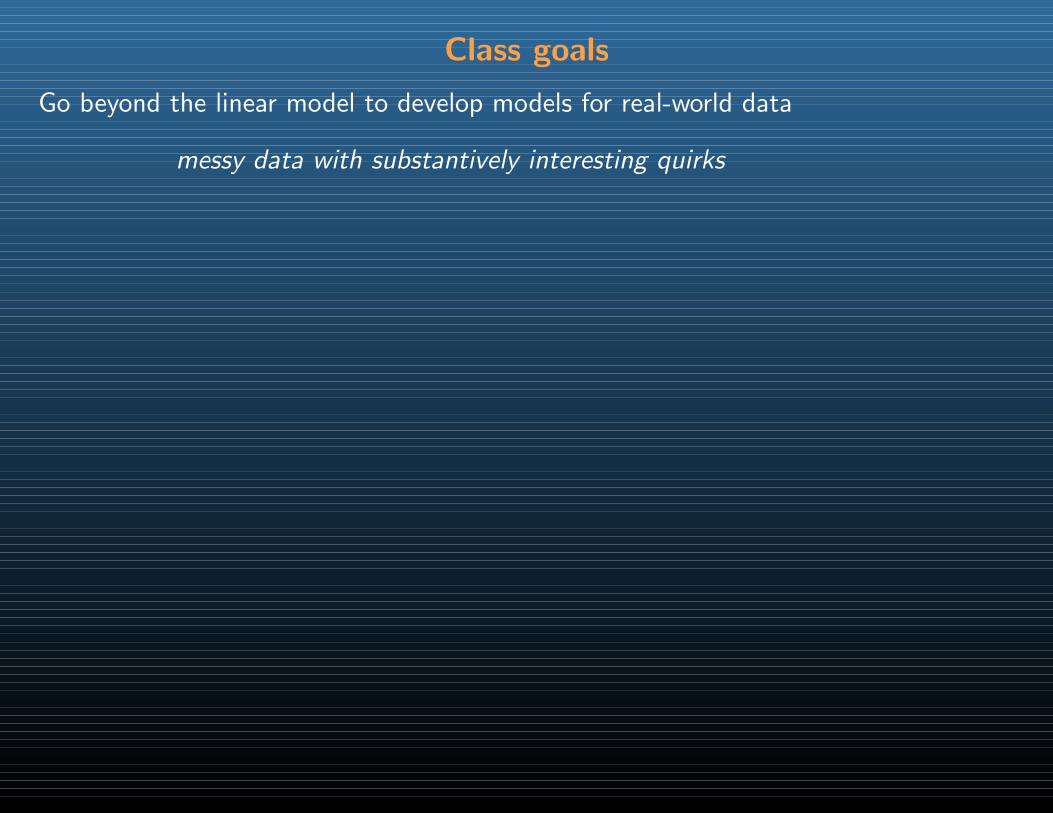
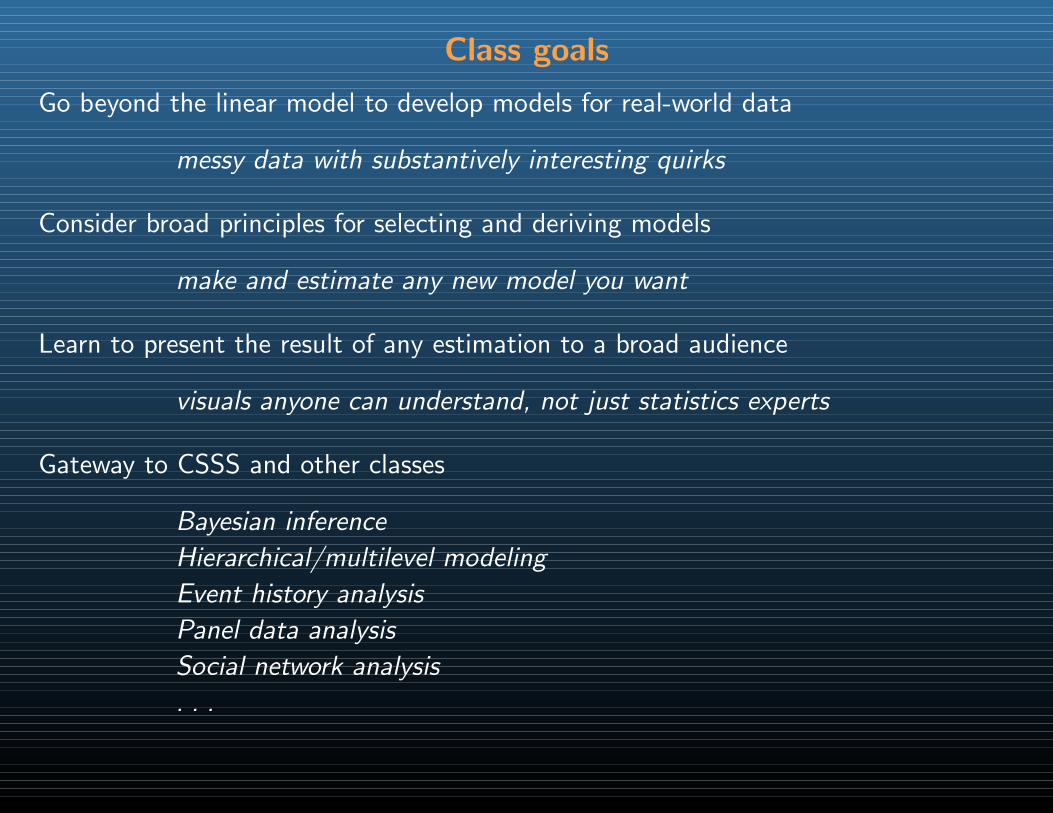
Go beyond the linear model to develop models for real-world data
messy data with substantively interesting quirks
Class goals
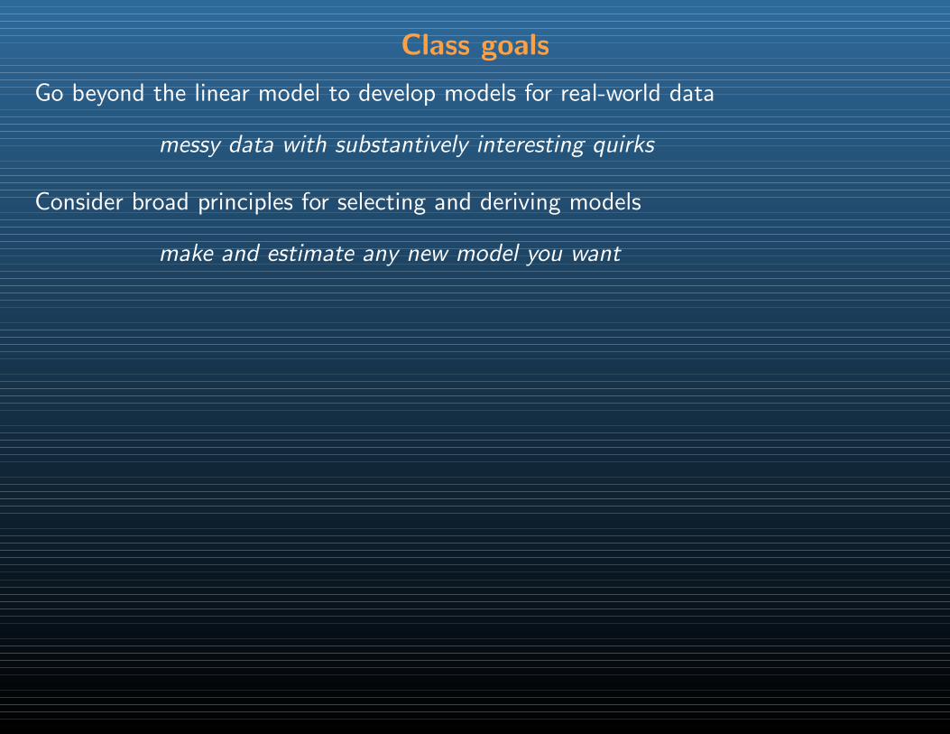
Go beyond the linear model to develop models for real-world data
messy data with substantively interesting quirks
Consider broad principles for selecting and deriving models
make and estimate any new model you want
Class goals
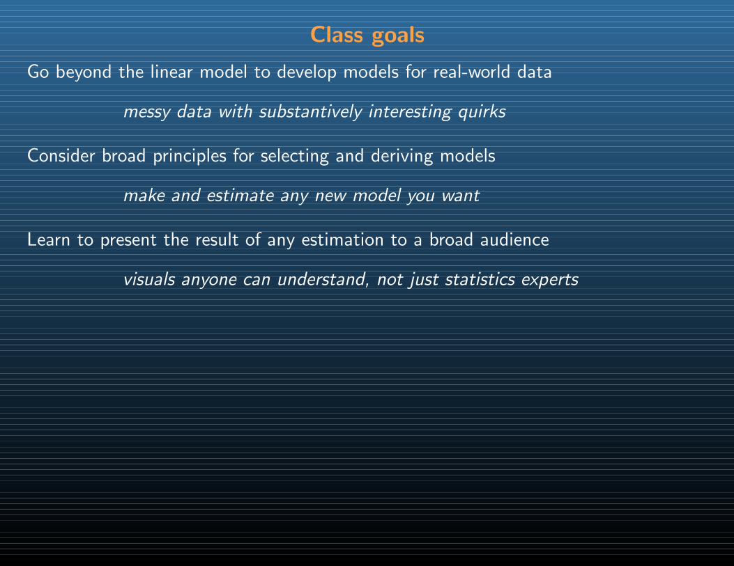
Go beyond the linear model to develop models for real-world data
messy data with substantively interesting quirks
Consider broad principles for selecting and deriving models
make and estimate any new model you want
Learn to present the result of any estimation to a broad audience
visuals anyone can understand, not just statistics experts
Class goals
Go beyond the linear model to develop models for real-world data
messy data with substantively interesting quirks
Consider broad principles for selecting and deriving models
make and estimate any new model you want
Learn to present the result of any estimation to a broad audience
visuals anyone can understand, not just statistics experts
Gateway to CSSS and other classes
Bayesian inference
Hierarchical/multilevel modeling
Event history analysis
Panel data analysis
Social network analysis
. . .

Challenges
1. Hard new concepts

Challenges
1. Hard new concepts
2. A fair bit of math
Challenges
1. Hard new concepts
2. A fair bit of math
3. Statistical programming rather than point-and-click

Payoff
1. Hard new concepts
Payoff
1. Hard new concepts
• Develop a more intuitive understanding of statistics
Payoff
1. Hard new concepts
• Develop a more intuitive understanding of statistics• Less “trust me;” more “show me”
Payoff
1. Hard new concepts
• Develop a more intuitive understanding of statistics• Less “trust me;” more “show me”• Get ready for advanced classes and independent study
Payoff
1. Hard new concepts
• Develop a more intuitive understanding of statistics• Less “trust me;” more “show me”• Get ready for advanced classes and independent study
2. A fair bit of math

Payoff
1. Hard new concepts
• Develop a more intuitive understanding of statistics• Less “trust me;” more “show me”• Get ready for advanced classes and independent study
2. A fair bit of math
• Unavoidable: we need the precision of mathematics

Payoff
1. Hard new concepts
• Develop a more intuitive understanding of statistics• Less “trust me;” more “show me”• Get ready for advanced classes and independent study
2. A fair bit of math
• Unavoidable: we need the precision of mathematics• You won’t be required to do proofs – but you may need to derive a new model

Payoff
1. Hard new concepts
• Develop a more intuitive understanding of statistics• Less “trust me;” more “show me”• Get ready for advanced classes and independent study
2. A fair bit of math
• Unavoidable: we need the precision of mathematics• You won’t be required to do proofs – but you may need to derive a new model• Numerical and visual alternatives where available
3. Statistical programming rather than point-and-click
• Steep learning curve, but in the end far more powerful

Payoff
1. Hard new concepts
• Develop a more intuitive understanding of statistics• Less “trust me;” more “show me”• Get ready for advanced classes and independent study
2. A fair bit of math
• Unavoidable: we need the precision of mathematics• You won’t be required to do proofs – but you may need to derive a new model• Numerical and visual alternatives where available
3. Statistical programming rather than point-and-click
• Steep learning curve, but in the end far more powerful• Great for applied research: bring the methods and data to the question
Payoff
1. Hard new concepts
• Develop a more intuitive understanding of statistics• Less “trust me;” more “show me”• Get ready for advanced classes and independent study
2. A fair bit of math
• Unavoidable: we need the precision of mathematics• You won’t be required to do proofs – but you may need to derive a new model• Numerical and visual alternatives where available
3. Statistical programming rather than point-and-click
• Steep learning curve, but in the end far more powerful• Great for applied research: bring the methods and data to the question• Empowering for any research involving data:
you’ll be surprised how many problems can be simplified by programming
MLE for Categorical & Count Data
First half of course focuses on inference about discrete data: categories & counts
Foundational quantitative methods classes focus on the linear regression model
• Assume data consist of a systematic component xiβ anda continuous, Normally distributed disturbance εi
• Easy to implement, estimate, and interpret
• A reasonable starting place for many analyses, with some robust features
But do the assumptions of linear regression (aka least squares) always fit?
Do they fit with discrete data?
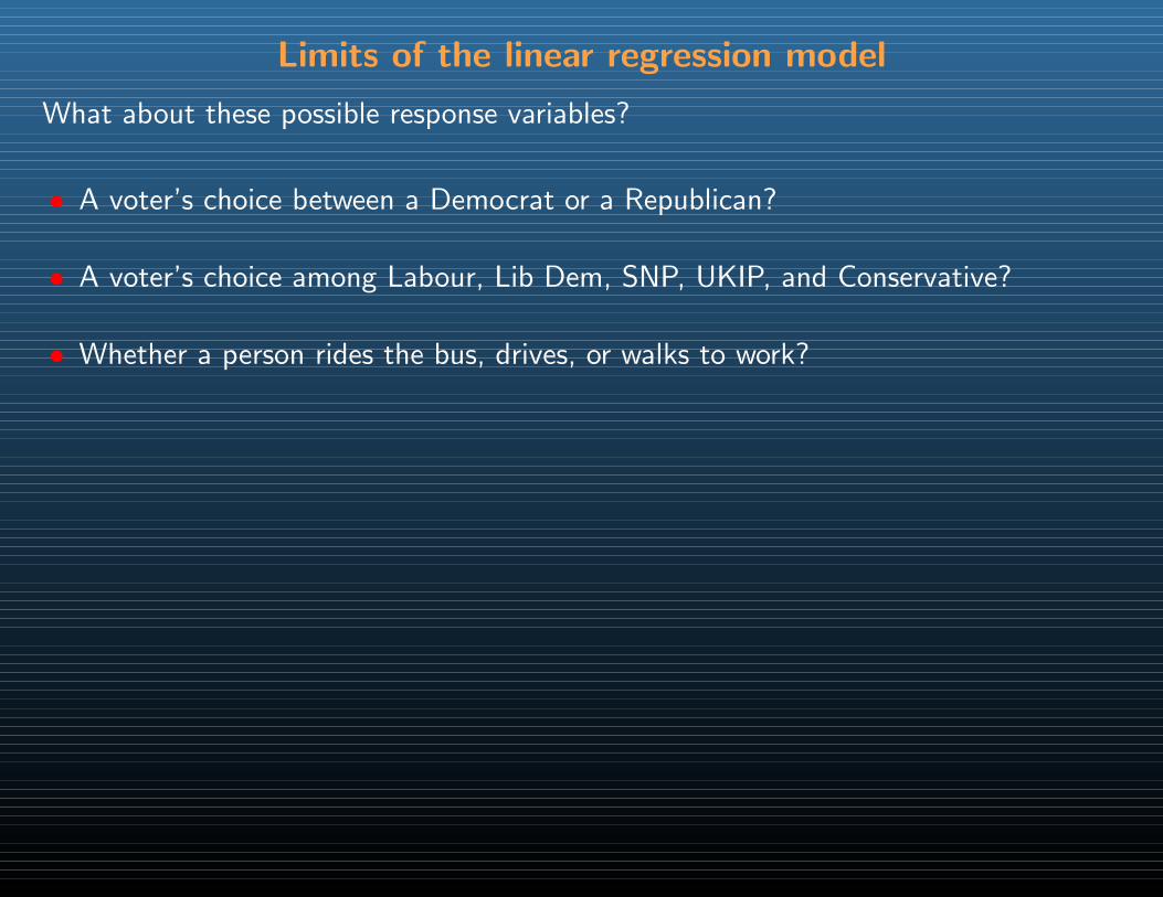
Limits of the linear regression model
What about these possible response variables?
• A voter’s choice between a Democrat or a Republican?
Limits of the linear regression model
What about these possible response variables?
• A voter’s choice between a Democrat or a Republican?
• A voter’s choice among Labour, Lib Dem, SNP, UKIP, and Conservative?
Limits of the linear regression model
What about these possible response variables?
• A voter’s choice between a Democrat or a Republican?
• A voter’s choice among Labour, Lib Dem, SNP, UKIP, and Conservative?
• Whether a person rides the bus, drives, or walks to work?
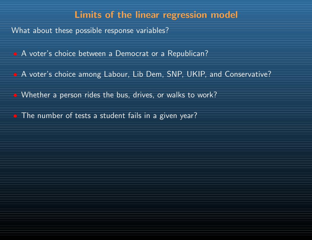
Limits of the linear regression model
What about these possible response variables?
• A voter’s choice between a Democrat or a Republican?
• A voter’s choice among Labour, Lib Dem, SNP, UKIP, and Conservative?
• Whether a person rides the bus, drives, or walks to work?
• The number of tests a student fails in a given year?
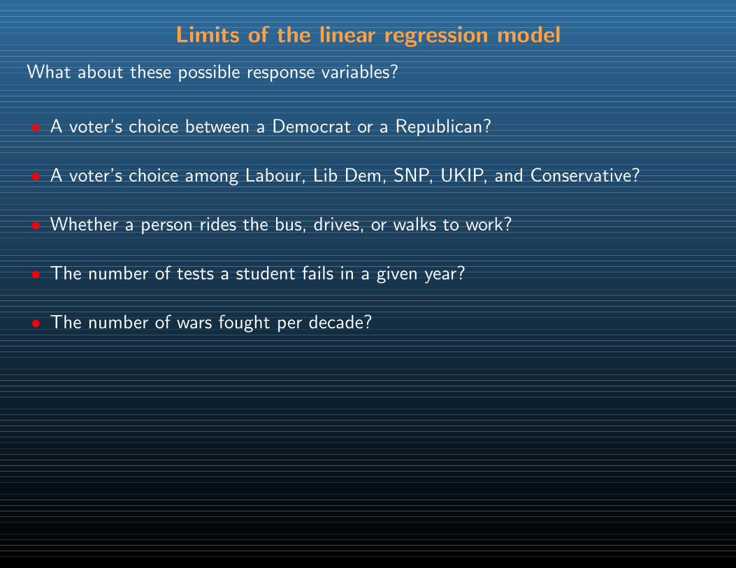
• The number of wars fought per decade?
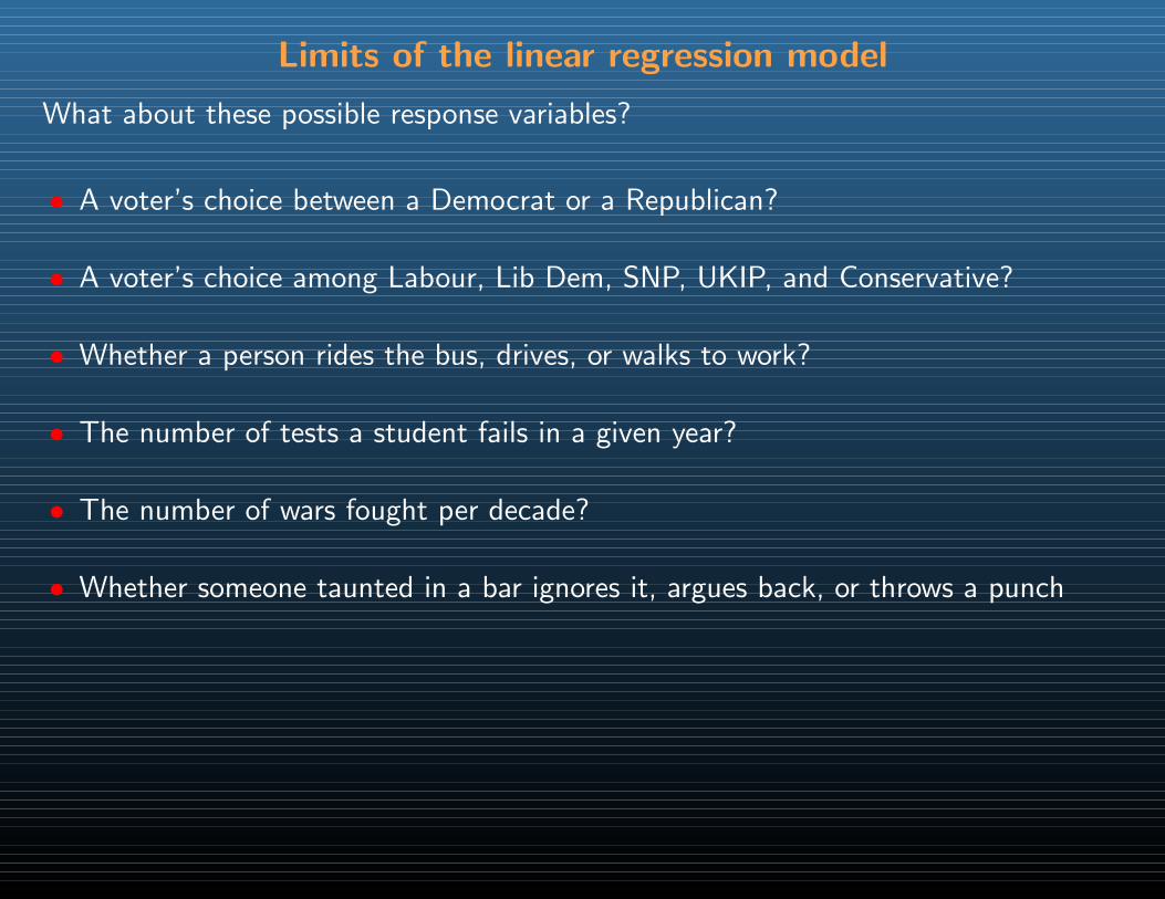
• Whether someone taunted in a bar ignores it, argues back, or throws a punch
Beyond linear regresion
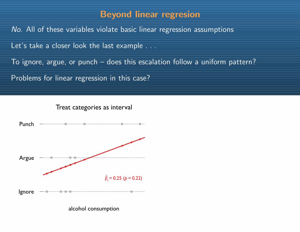
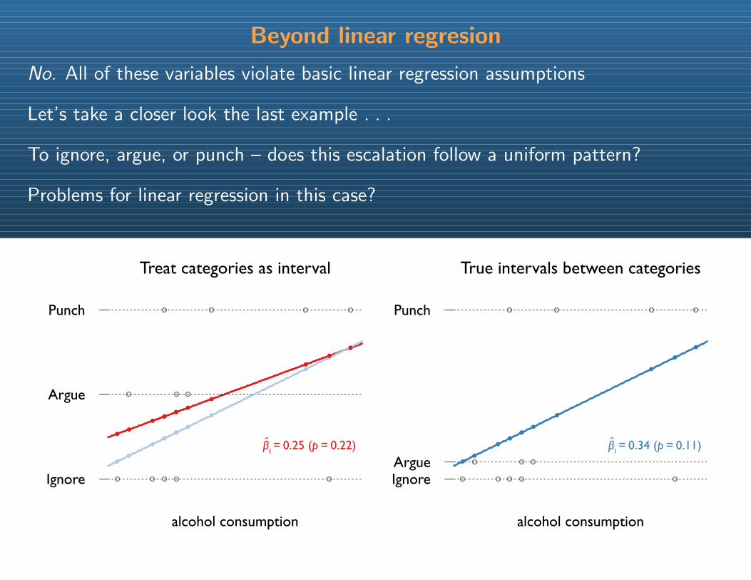
No. All of these variables violate basic linear regression assumptions
Beyond linear regresion
No. All of these variables violate basic linear regression assumptions
Let’s take a closer look the last example . . .
To ignore, argue, or punch – does this escalation follow a uniform pattern?
Problems for linear regression in this case?
Ignore
Argue
Punch
Treat categories as interval
alcohol consumption
β1 = 0.25 (p = 0.22)
Beyond linear regresion
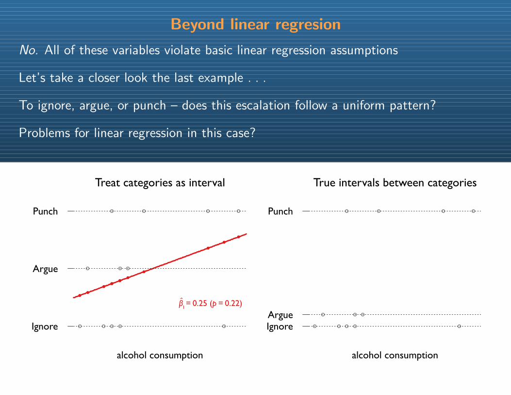
No. All of these variables violate basic linear regression assumptions
Let’s take a closer look the last example . . .
To ignore, argue, or punch – does this escalation follow a uniform pattern?
Problems for linear regression in this case?
Ignore
Argue
Punch
Treat categories as interval
alcohol consumption
IgnoreArgue
Punch
True intervals between categories
alcohol consumption
β1 = 0.25 (p = 0.22)
Beyond linear regresion
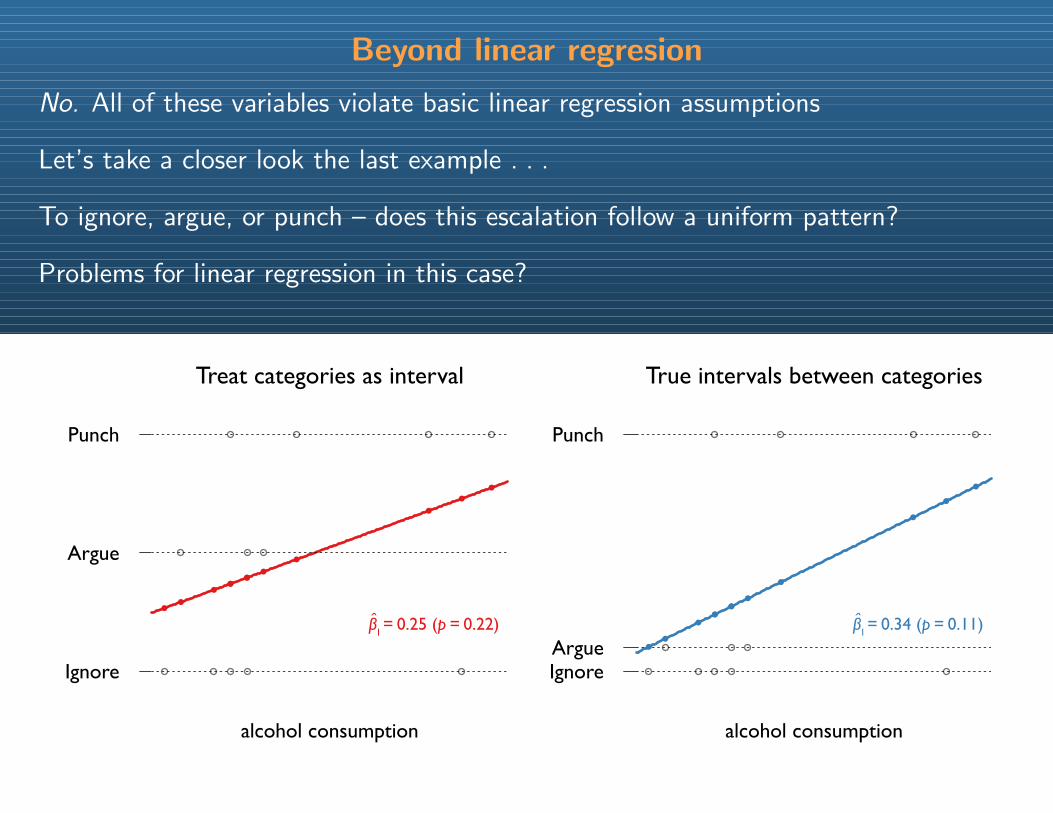
No. All of these variables violate basic linear regression assumptions
Let’s take a closer look the last example . . .
To ignore, argue, or punch – does this escalation follow a uniform pattern?
Problems for linear regression in this case?
Ignore
Argue
Punch
Treat categories as interval
alcohol consumption
IgnoreArgue
Punch
True intervals between categories
alcohol consumption
β1 = 0.25 (p = 0.22) β1 = 0.34 (p = 0.11)
Beyond linear regresion
No. All of these variables violate basic linear regression assumptions
Let’s take a closer look the last example . . .
To ignore, argue, or punch – does this escalation follow a uniform pattern?
Problems for linear regression in this case?
Ignore
Argue
Punch
Treat categories as interval
alcohol consumption
IgnoreArgue
Punch
True intervals between categories
alcohol consumption
β1 = 0.25 (p = 0.22) β1 = 0.34 (p = 0.11)
Beyond linear regression
In this class, you’ll learn three things:
Beyond linear regression
In this class, you’ll learn three things:
Theory: Probability models to deal with discrete and categorical data
Beyond linear regression
In this class, you’ll learn three things:
Theory: Probability models to deal with discrete and categorical data
Application: Selecting and presenting models to uncover substantive relationships
Beyond linear regression
In this class, you’ll learn three things:
Theory: Probability models to deal with discrete and categorical data
Application: Selecting and presenting models to uncover substantive relationships
Practice: Programming skills to implement, fit, and interpret these models

Getting started
In particular, we’ll follow a four step procedure:
Getting started
In particular, we’ll follow a four step procedure:
1. Identify a probability model for a dependent variable
Getting started
In particular, we’ll follow a four step procedure:
1. Identify a probability model for a dependent variable
2. Derive an estimator for it
Getting started
In particular, we’ll follow a four step procedure:
1. Identify a probability model for a dependent variable
2. Derive an estimator for it
3. Fit the model and check the goodness of fit
Getting started
In particular, we’ll follow a four step procedure:
1. Identify a probability model for a dependent variable
2. Derive an estimator for it
3. Fit the model and check the goodness of fit
4. Interpret the results, usually graphically
Getting started
In particular, we’ll follow a four step procedure:
1. Identify a probability model for a dependent variable
2. Derive an estimator for it
3. Fit the model and check the goodness of fit
4. Interpret the results, usually graphically
We’ll start on Step 1 today . . .
Outline for today
1. Course administration
2. Review basic probability
3. Review some fundamental probability distributions

Course administration
1. Syllabus
2. Paper requirements
3. Survey
4. Introductions
Lightning course in basic probability: Sets
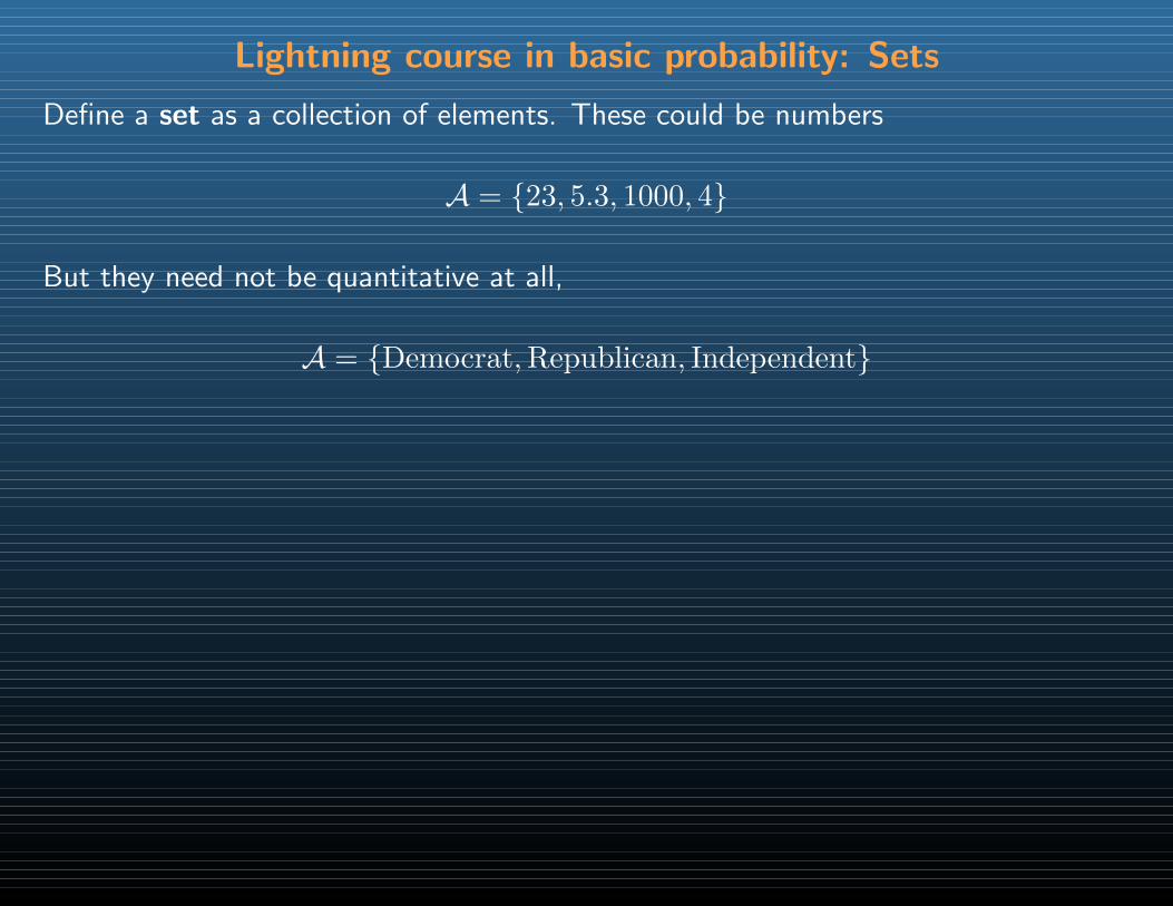
Define a set as a collection of elements. These could be numbers
A = 23, 5.3, 1000, 4
Lightning course in basic probability: Sets
Define a set as a collection of elements. These could be numbers
A = 23, 5.3, 1000, 4
But they need not be quantitative at all,
A = Democrat,Republican, Independent
Lightning course in basic probability: Sets
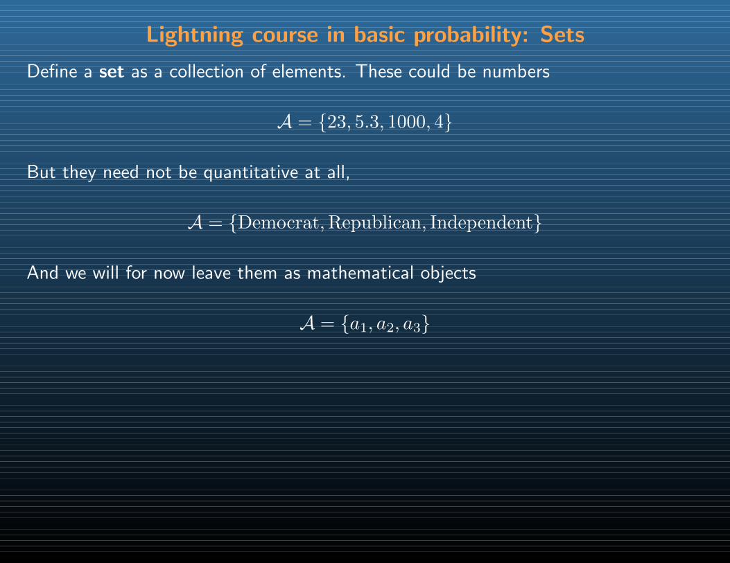
Define a set as a collection of elements. These could be numbers
A = 23, 5.3, 1000, 4
But they need not be quantitative at all,
A = Democrat,Republican, Independent
And we will for now leave them as mathematical objects
A = a1, a2, a3
Lightning course in basic probability: Sets
Define a set as a collection of elements. These could be numbers
A = 23, 5.3, 1000, 4
But they need not be quantitative at all,
A = Democrat,Republican, Independent
And we will for now leave them as mathematical objects
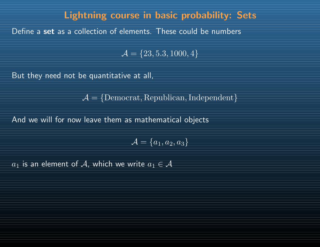
A = a1, a2, a3
a1 is an element of A, which we write a1 ∈ A
Lightning course in basic probability: Sets
Define a set as a collection of elements. These could be numbers
A = 23, 5.3, 1000, 4
But they need not be quantitative at all,
A = Democrat,Republican, Independent
And we will for now leave them as mathematical objects
A = a1, a2, a3
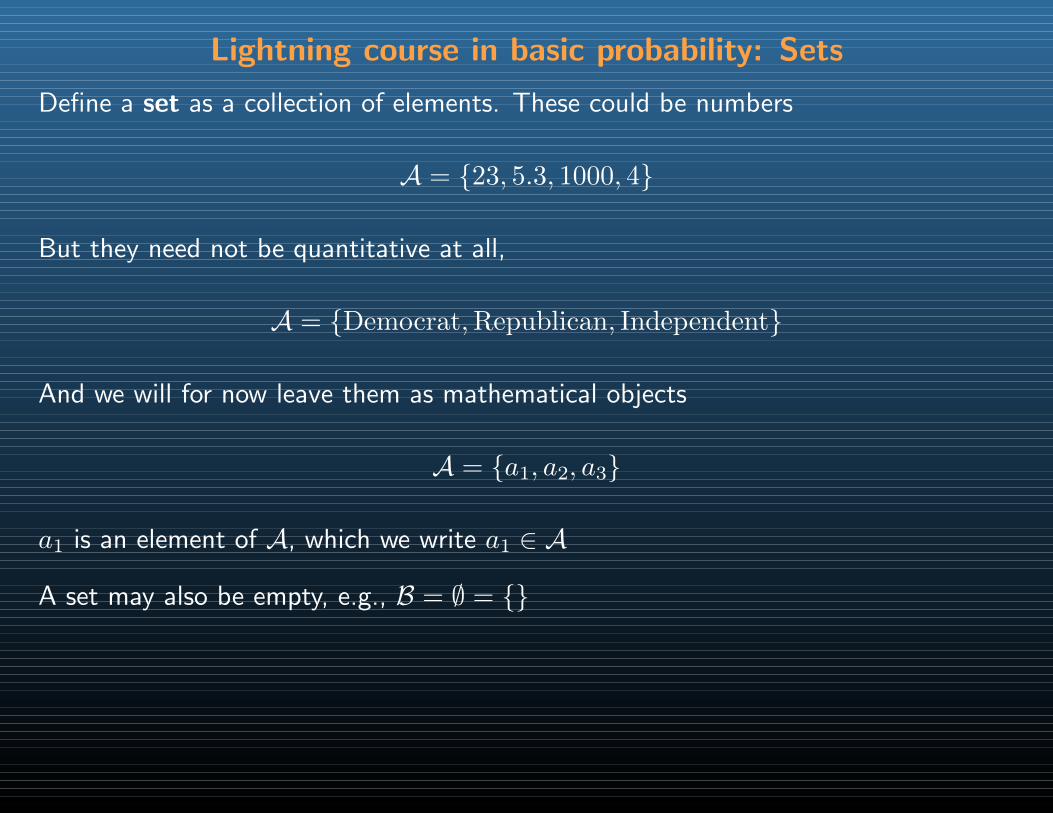
a1 is an element of A, which we write a1 ∈ A
A set may also be empty, e.g., B = ∅ =
Lightning course in basic probability: Sets
We define 3 basic set operators:
subset ⊂ union ∪ intersection ∩
Lightning course in basic probability: Sets
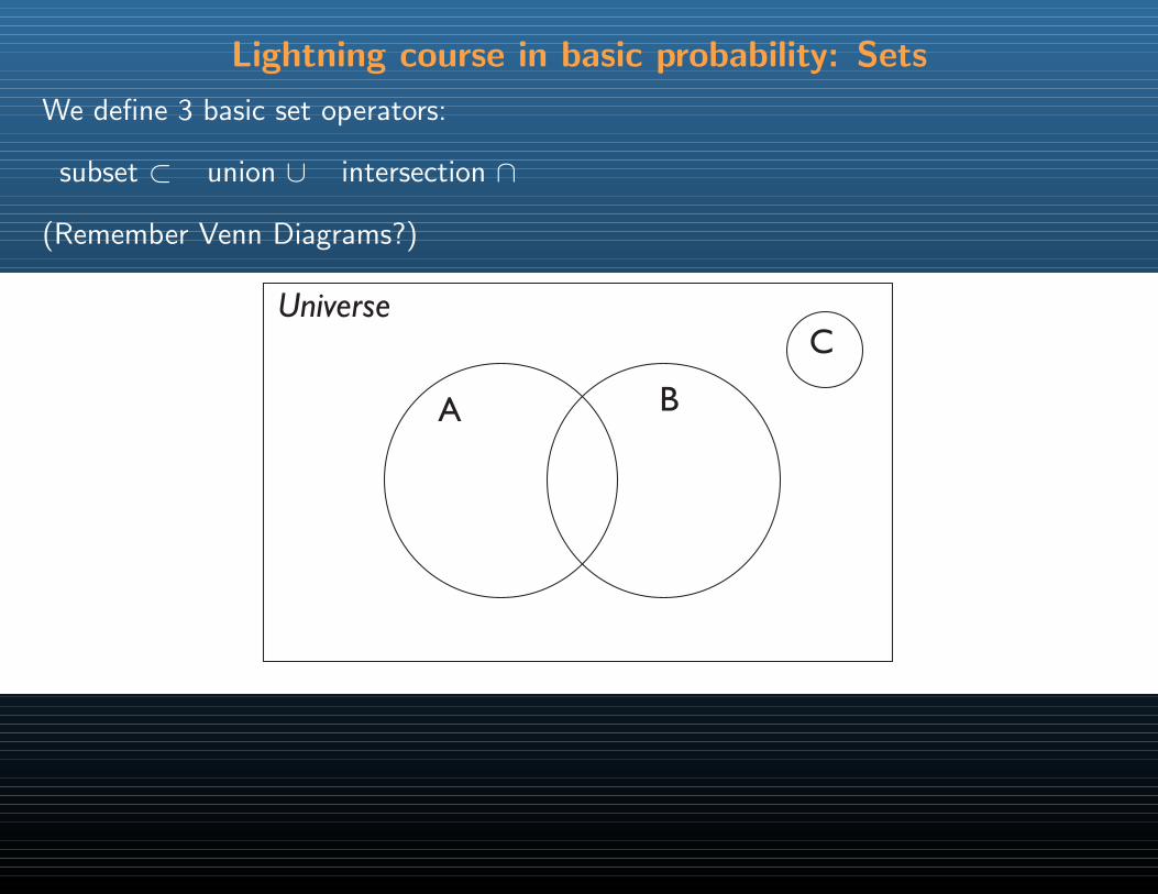
We define 3 basic set operators:
subset ⊂ union ∪ intersection ∩
(Remember Venn Diagrams?)
Universe
A B
C
Lightning course in basic probability: Sets
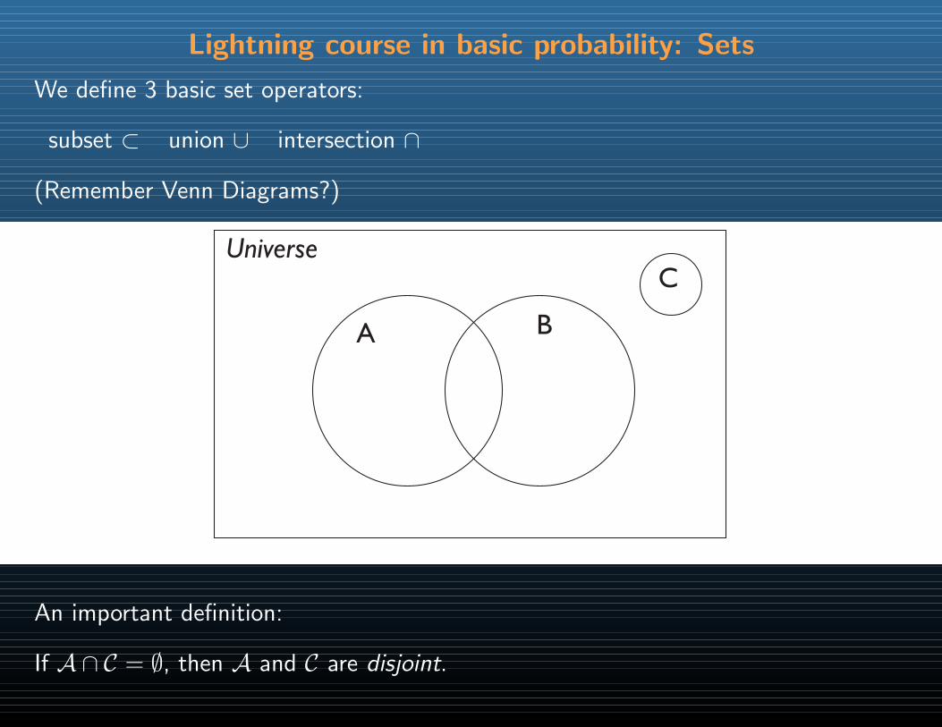
We define 3 basic set operators:
subset ⊂ union ∪ intersection ∩
(Remember Venn Diagrams?)
Universe
A B
C
An important definition:
If A ∩ C = ∅, then A and C are disjoint.
Lightning course in basic probability: Probability
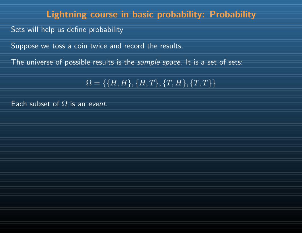
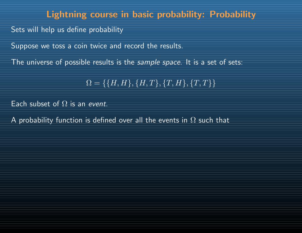
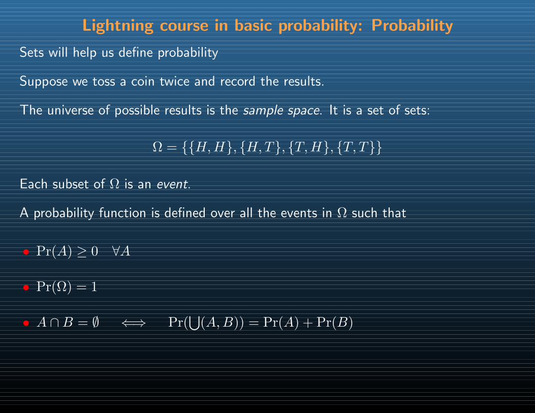
Sets will help us define probability
Suppose we toss a coin twice and record the results.
Lightning course in basic probability: Probability
Sets will help us define probability
Suppose we toss a coin twice and record the results.
The universe of possible results is the sample space. It is a set of sets:
Ω = H,H, H,T, T,H, T, T
Each subset of Ω is an event.
Lightning course in basic probability: Probability
Sets will help us define probability
Suppose we toss a coin twice and record the results.
The universe of possible results is the sample space. It is a set of sets:
Ω = H,H, H,T, T,H, T, T
Each subset of Ω is an event.
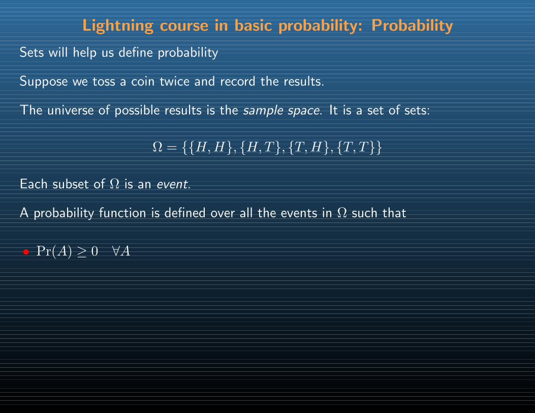
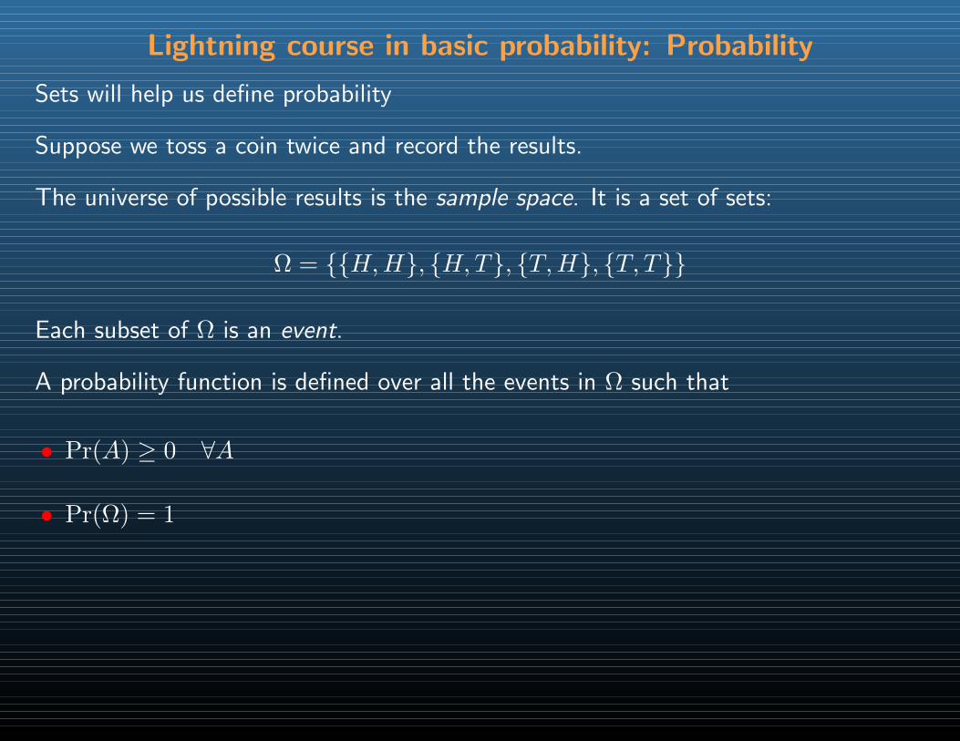
A probability function is defined over all the events in Ω such that
Lightning course in basic probability: Probability
Sets will help us define probability
Suppose we toss a coin twice and record the results.
The universe of possible results is the sample space. It is a set of sets:
Ω = H,H, H,T, T,H, T, T
Each subset of Ω is an event.
A probability function is defined over all the events in Ω such that
• Pr(A) ≥ 0 ∀A
• Pr(Ω) = 1
• A ∩B = ∅ ⇐⇒ Pr(⋃
(A,B)) = Pr(A) + Pr(B)
Lightning course in basic probability: Probability
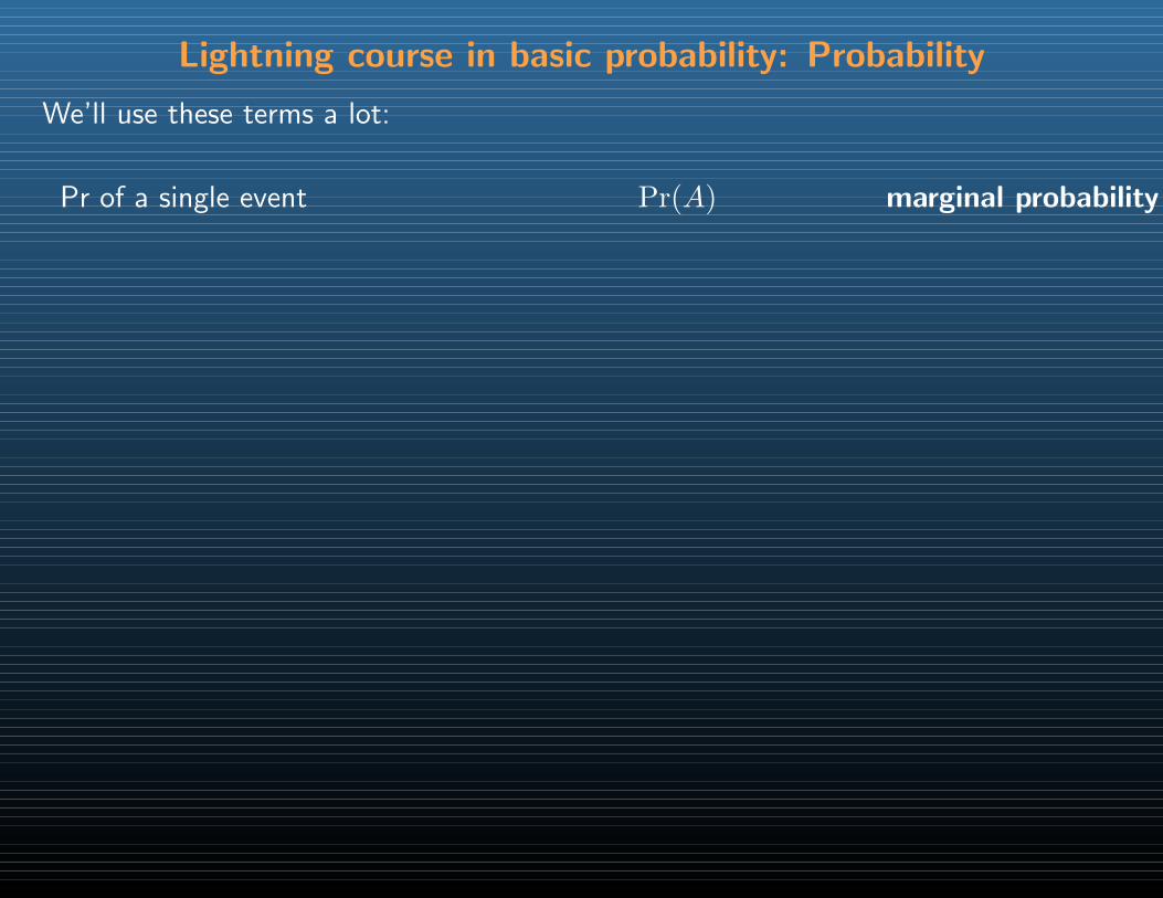
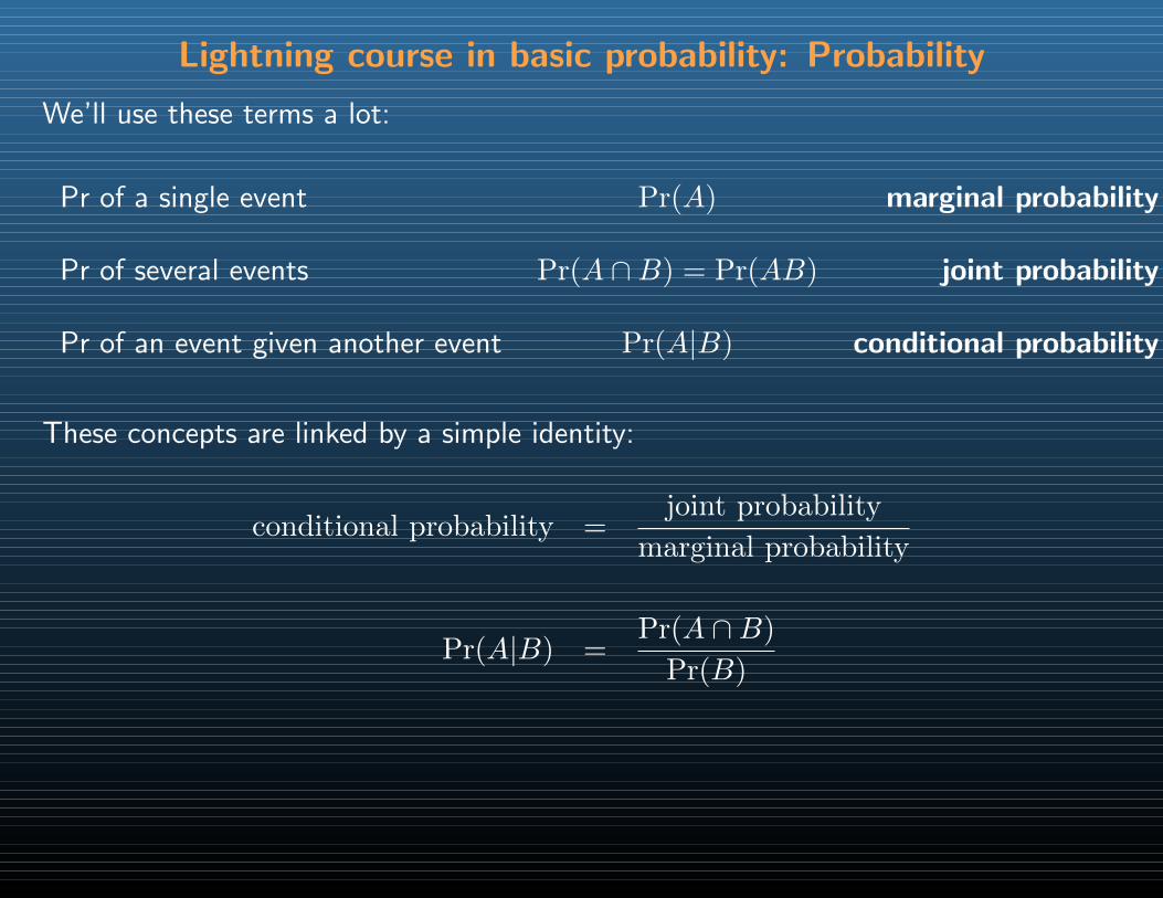
We’ll use these terms a lot:
Pr of a single event Pr(A) marginal probability
Lightning course in basic probability: Probability
We’ll use these terms a lot:
Pr of a single event Pr(A) marginal probability
Pr of several events Pr(A ∩B) = Pr(AB) joint probability
Lightning course in basic probability: Probability
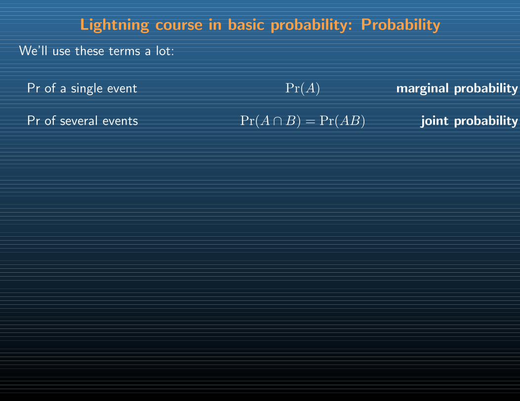
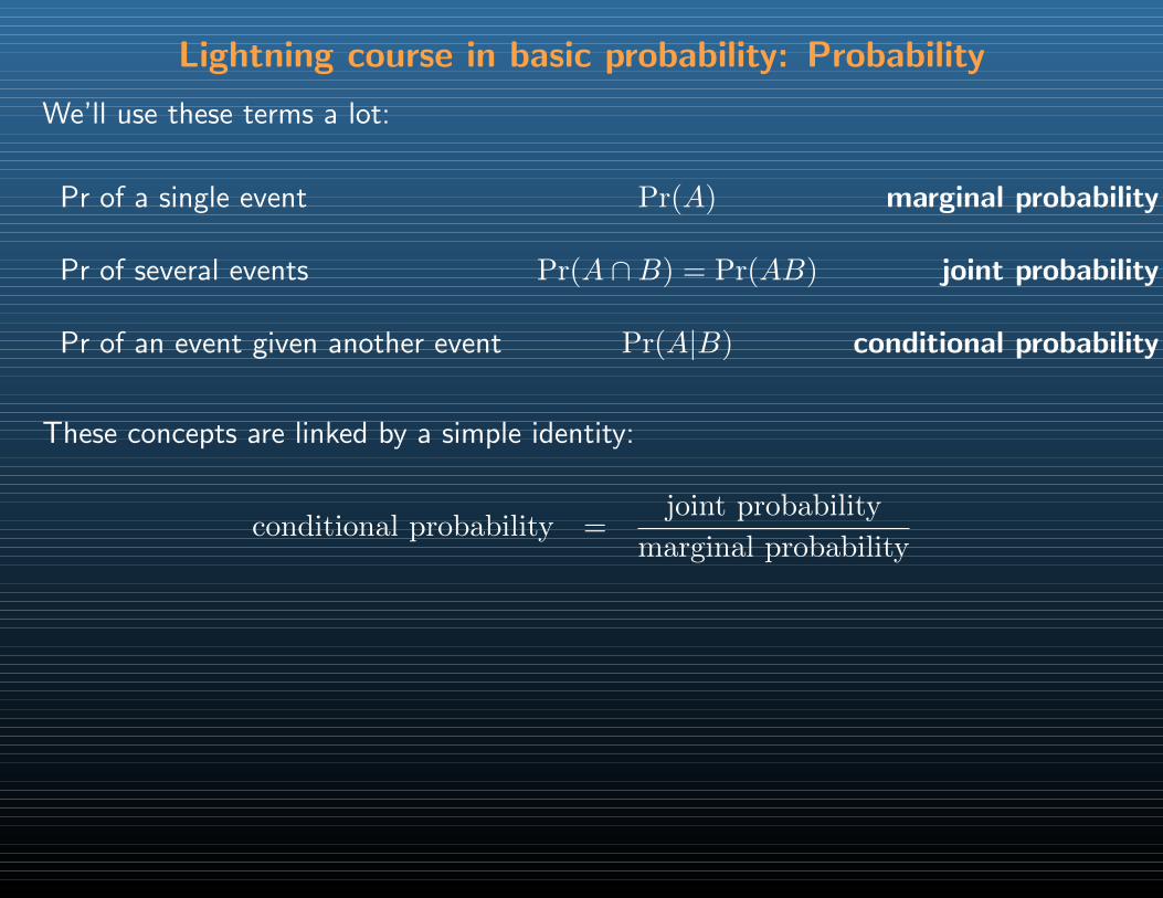
We’ll use these terms a lot:
Pr of a single event Pr(A) marginal probability
Pr of several events Pr(A ∩B) = Pr(AB) joint probability
Pr of an event given another event Pr(A|B) conditional probability
These concepts are linked by a simple identity:
conditional probability =joint probability
marginal probability
Lightning course in basic probability: Probability
We’ll use these terms a lot:
Pr of a single event Pr(A) marginal probability
Pr of several events Pr(A ∩B) = Pr(AB) joint probability
Pr of an event given another event Pr(A|B) conditional probability
These concepts are linked by a simple identity:
conditional probability =joint probability
marginal probability
Pr(A|B) =Pr(A ∩B)
Pr(B)
Lightning course in basic probability: Probability
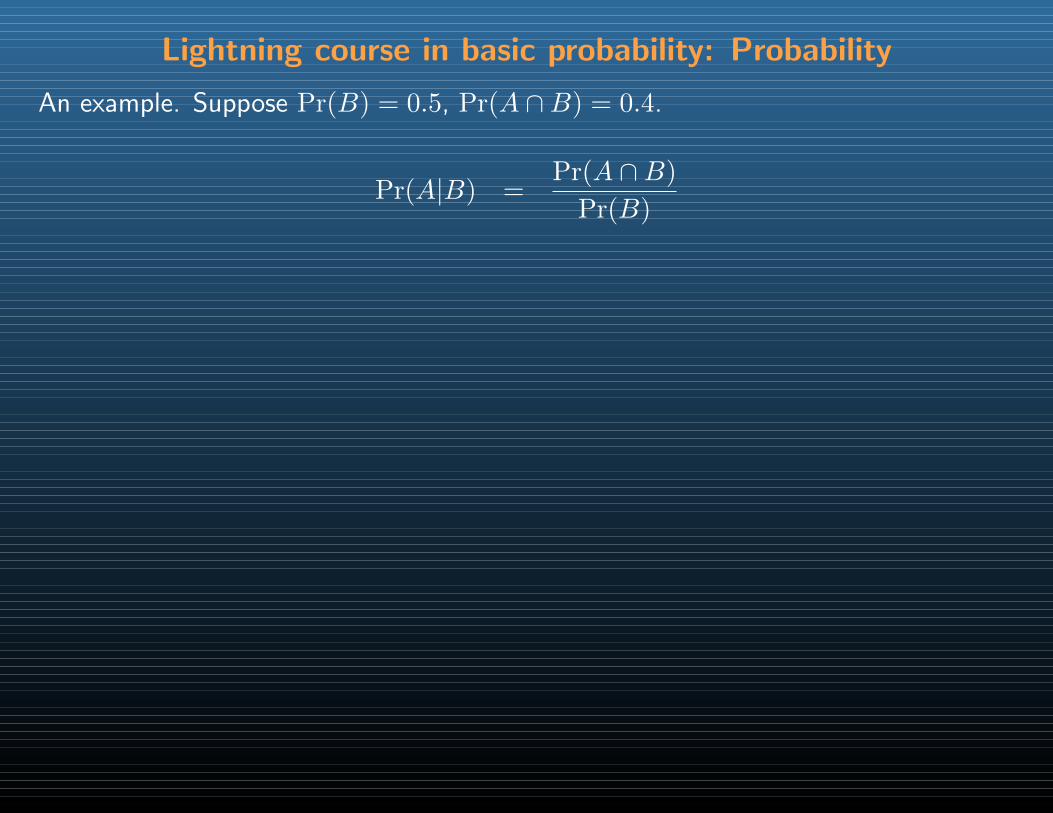
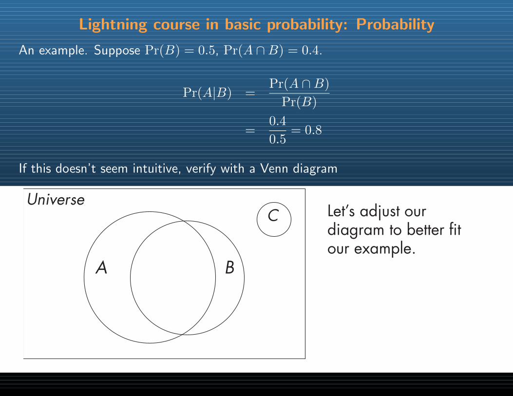
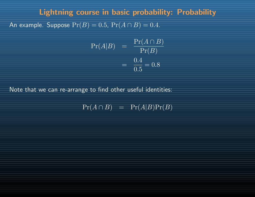
An example. Suppose Pr(B) = 0.5, Pr(A ∩B) = 0.4.
Pr(A|B) =Pr(A ∩B)
Pr(B)
Lightning course in basic probability: Probability
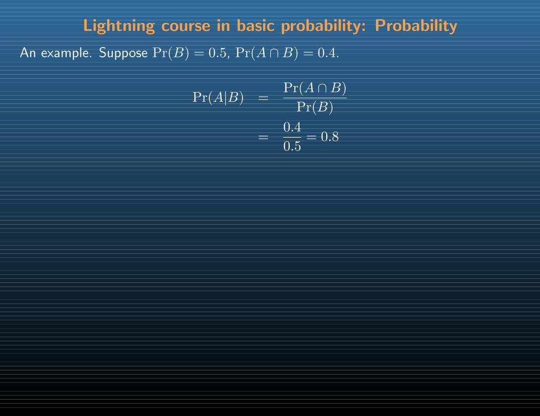
An example. Suppose Pr(B) = 0.5, Pr(A ∩B) = 0.4.
Pr(A|B) =Pr(A ∩B)
Pr(B)
=0.4
0.5= 0.8
Lightning course in basic probability: Probability
An example. Suppose Pr(B) = 0.5, Pr(A ∩B) = 0.4.
Pr(A|B) =Pr(A ∩B)
Pr(B)
=0.4
0.5= 0.8
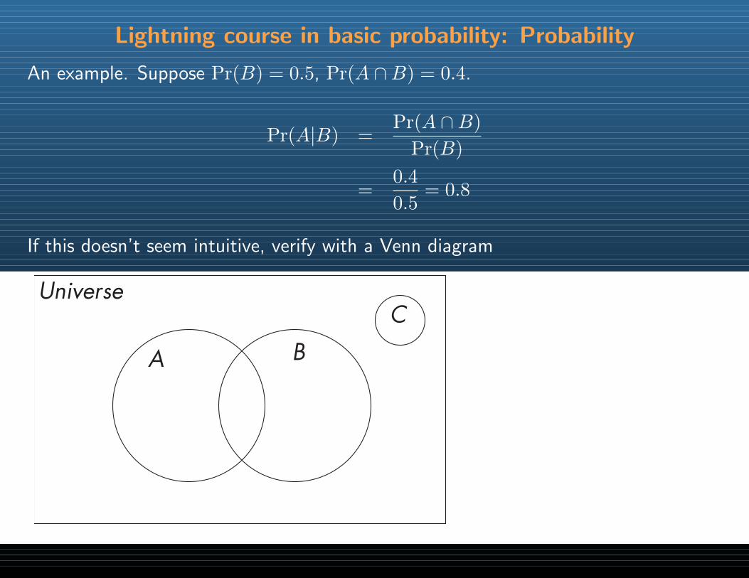
If this doesn’t seem intuitive, verify with a Venn diagram
Universe
A B
C
Lightning course in basic probability: Probability
An example. Suppose Pr(B) = 0.5, Pr(A ∩B) = 0.4.
Pr(A|B) =Pr(A ∩B)
Pr(B)
=0.4
0.5= 0.8
If this doesn’t seem intuitive, verify with a Venn diagram
Universe
A B
C Let’s adjust our diagram to better fit our example.
Lightning course in basic probability: Probability
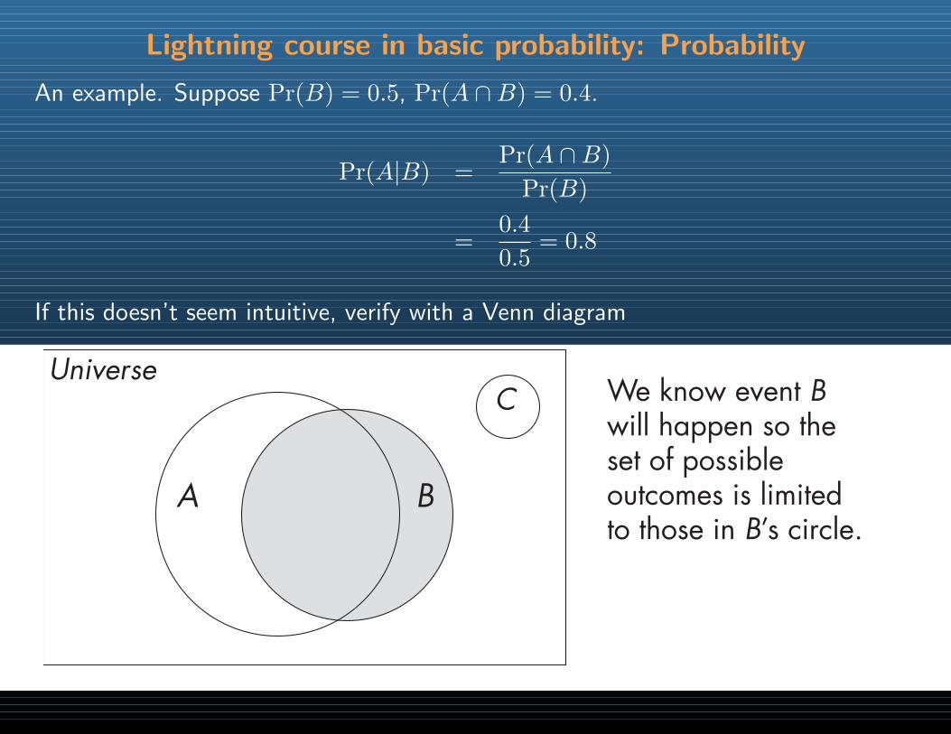
An example. Suppose Pr(B) = 0.5, Pr(A ∩B) = 0.4.
Pr(A|B) =Pr(A ∩B)
Pr(B)
=0.4
0.5= 0.8
If this doesn’t seem intuitive, verify with a Venn diagram
Universe
A B
C We know event B will happen so the set of possible outcomes is limited to those in B’s circle.
Lightning course in basic probability: Probability
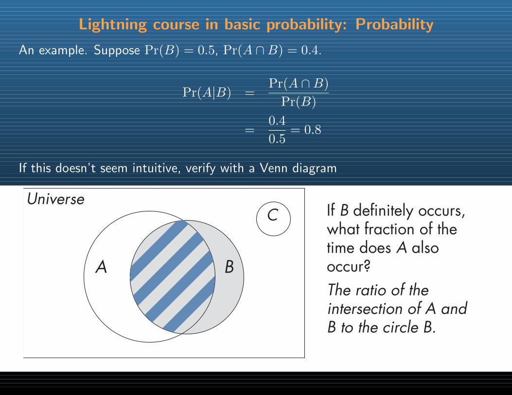
An example. Suppose Pr(B) = 0.5, Pr(A ∩B) = 0.4.
Pr(A|B) =Pr(A ∩B)
Pr(B)
=0.4
0.5= 0.8
If this doesn’t seem intuitive, verify with a Venn diagram
Universe
A B
C If B definitely occurs, what fraction of the time does A also occur?The ratio of the intersection of A and B to the circle B.
Lightning course in basic probability: Probability
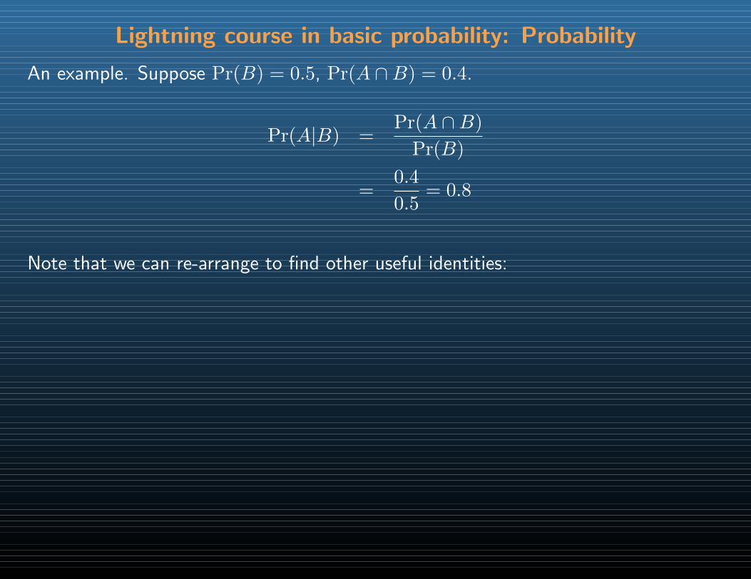
An example. Suppose Pr(B) = 0.5, Pr(A ∩B) = 0.4.
Pr(A|B) =Pr(A ∩B)
Pr(B)
=0.4
0.5= 0.8
Note that we can re-arrange to find other useful identities:
Lightning course in basic probability: Probability
An example. Suppose Pr(B) = 0.5, Pr(A ∩B) = 0.4.
Pr(A|B) =Pr(A ∩B)
Pr(B)
=0.4
0.5= 0.8
Note that we can re-arrange to find other useful identities:
Pr(A ∩B) = Pr(A|B)Pr(B)
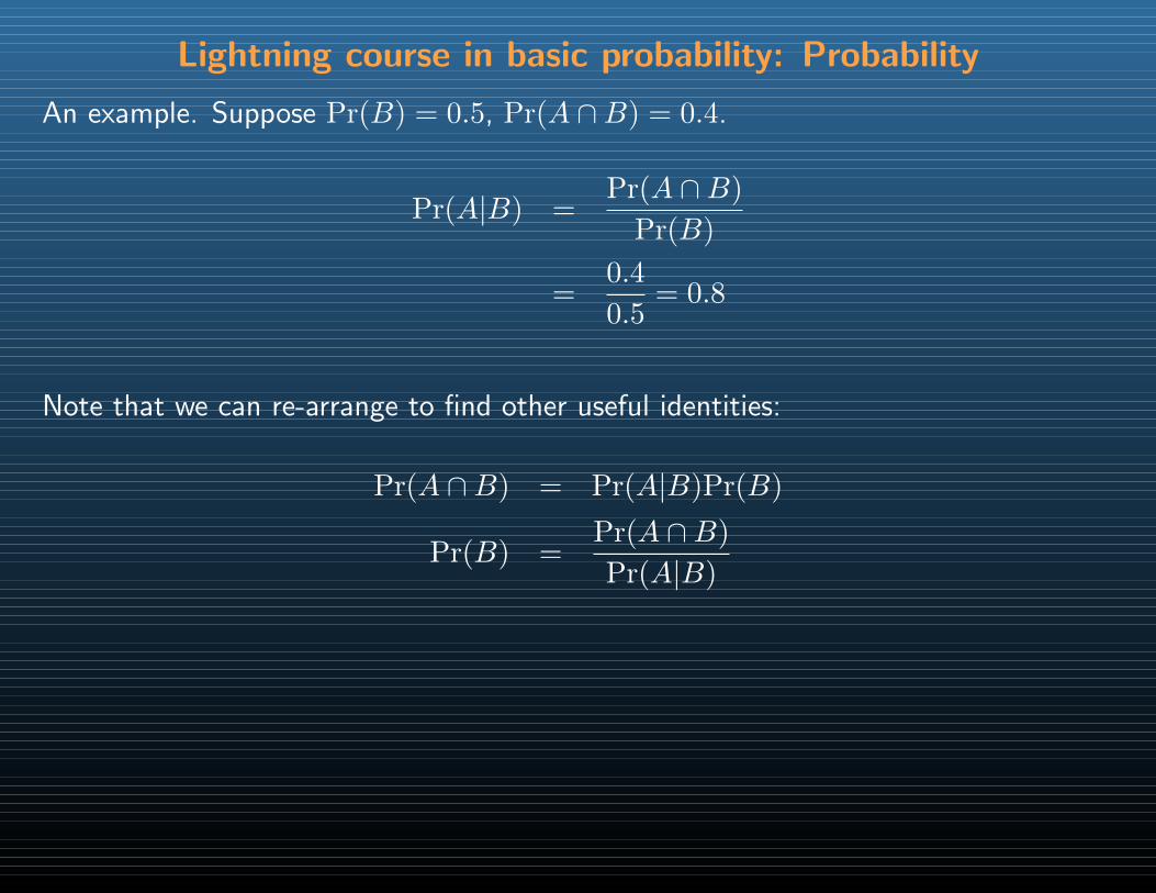
Lightning course in basic probability: Probability
An example. Suppose Pr(B) = 0.5, Pr(A ∩B) = 0.4.
Pr(A|B) =Pr(A ∩B)
Pr(B)
=0.4
0.5= 0.8
Note that we can re-arrange to find other useful identities:
Pr(A ∩B) = Pr(A|B)Pr(B)
Pr(B) =Pr(A ∩B)
Pr(A|B)
Lightning course in basic probability: Probability
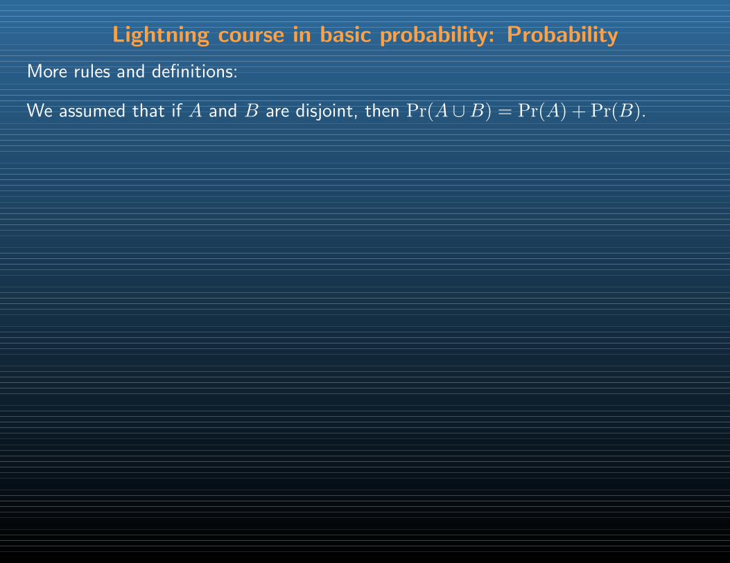
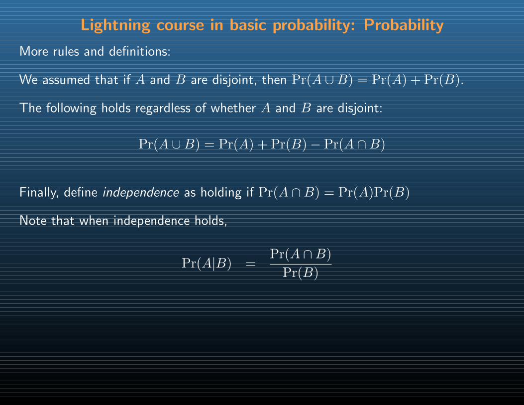
More rules and definitions:
We assumed that if A and B are disjoint, then Pr(A ∪B) = Pr(A) + Pr(B).
Lightning course in basic probability: Probability
More rules and definitions:
We assumed that if A and B are disjoint, then Pr(A ∪B) = Pr(A) + Pr(B).
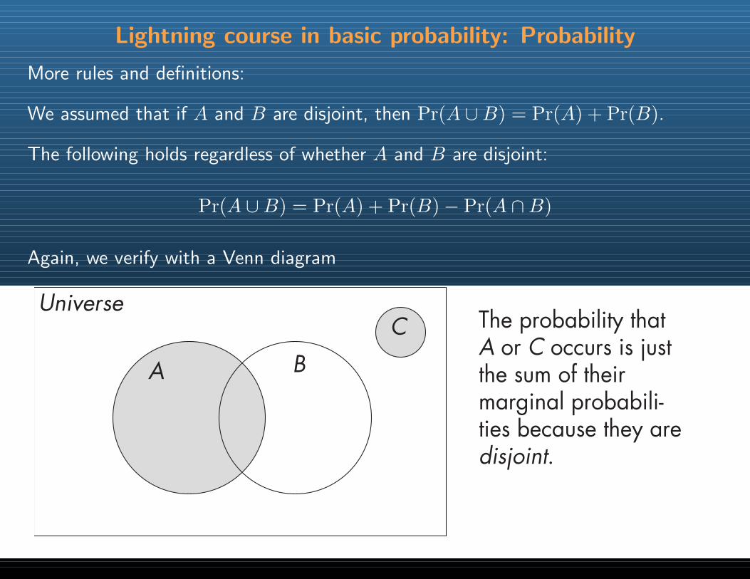
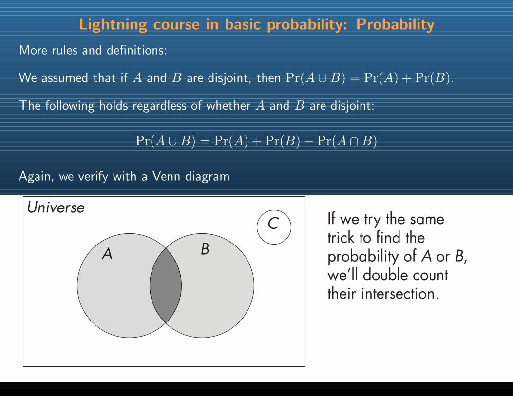
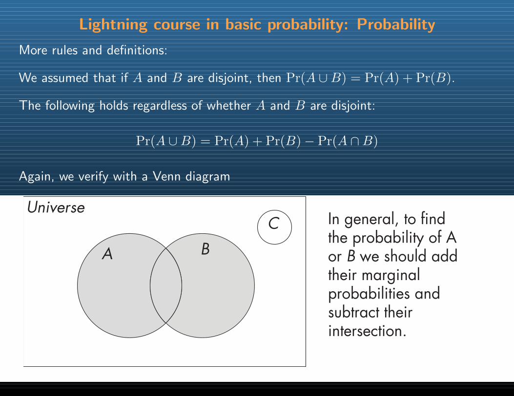
The following holds regardless of whether A and B are disjoint:
Pr(A ∪B) = Pr(A) + Pr(B)− Pr(A ∩B)
Lightning course in basic probability: Probability
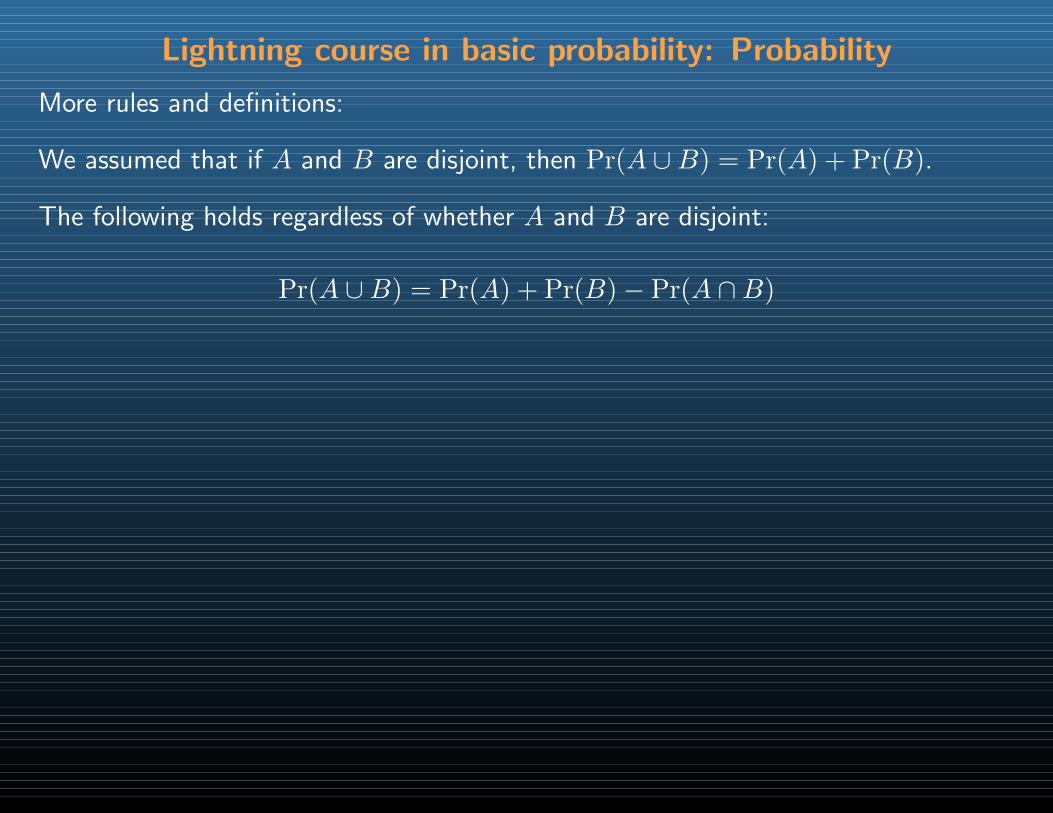
More rules and definitions:
We assumed that if A and B are disjoint, then Pr(A ∪B) = Pr(A) + Pr(B).
The following holds regardless of whether A and B are disjoint:
Pr(A ∪B) = Pr(A) + Pr(B)− Pr(A ∩B)
Again, we verify with a Venn diagram
Universe
A B
C The probability that A or C occurs is just the sum of their marginal probabili-ties because they are disjoint.
Lightning course in basic probability: Probability
More rules and definitions:
We assumed that if A and B are disjoint, then Pr(A ∪B) = Pr(A) + Pr(B).
The following holds regardless of whether A and B are disjoint:
Pr(A ∪B) = Pr(A) + Pr(B)− Pr(A ∩B)
Again, we verify with a Venn diagram
Universe
A B
C If we try the same trick to find the probability of A or B, we’ll double count their intersection.
Lightning course in basic probability: Probability
More rules and definitions:
We assumed that if A and B are disjoint, then Pr(A ∪B) = Pr(A) + Pr(B).
The following holds regardless of whether A and B are disjoint:
Pr(A ∪B) = Pr(A) + Pr(B)− Pr(A ∩B)
Again, we verify with a Venn diagram
Universe
A B
C In general, to find the probability of A or B we should add their marginal probabilities and subtract their intersection.
Lightning course in basic probability: Probability
More rules and definitions:
We assumed that if A and B are disjoint, then Pr(A ∪B) = Pr(A) + Pr(B).
The following holds regardless of whether A and B are disjoint:
Pr(A ∪B) = Pr(A) + Pr(B)− Pr(A ∩B)
Finally, define independence as holding if Pr(A ∩B) = Pr(A)Pr(B)
Note that when independence holds,
Pr(A|B) =Pr(A ∩B)
Pr(B)
Lightning course in basic probability: Probability
More rules and definitions:
We assumed that if A and B are disjoint, then Pr(A ∪B) = Pr(A) + Pr(B).
The following holds regardless of whether A and B are disjoint:
Pr(A ∪B) = Pr(A) + Pr(B)− Pr(A ∩B)
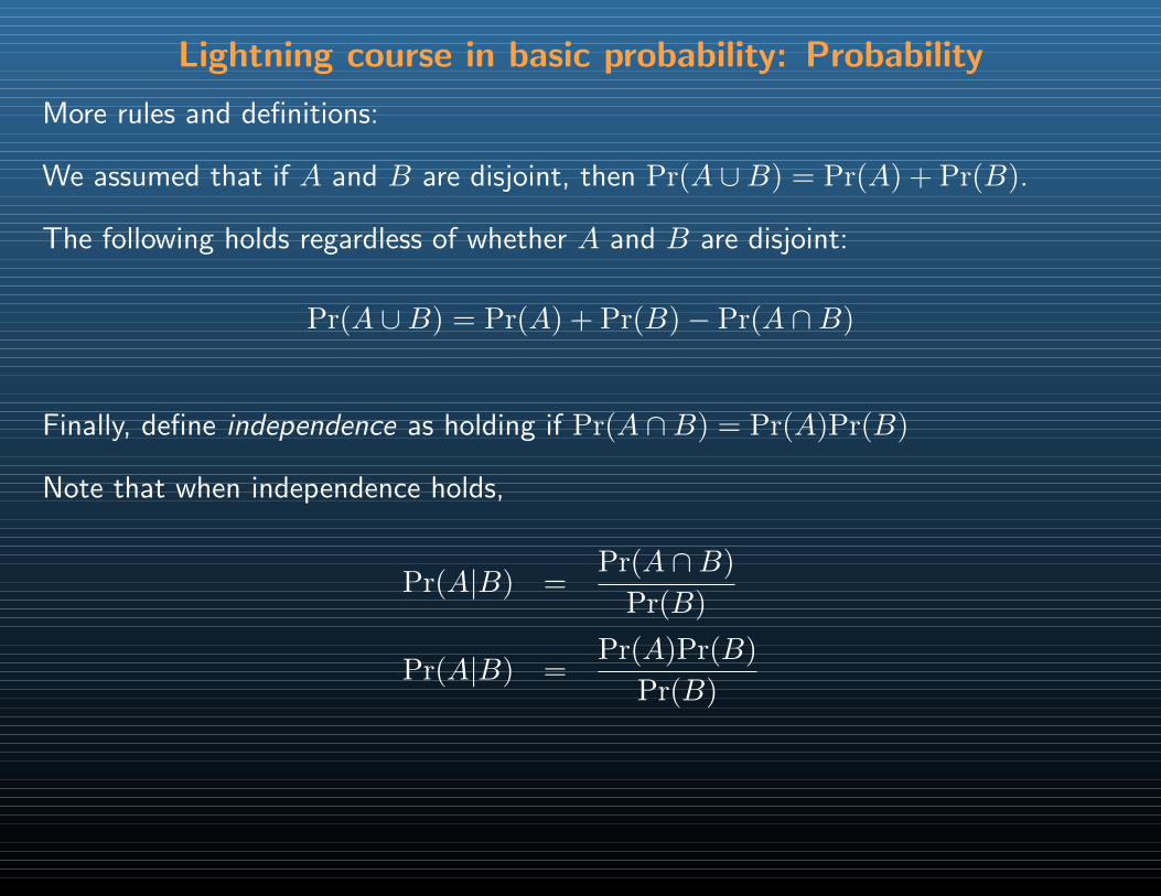
Finally, define independence as holding if Pr(A ∩B) = Pr(A)Pr(B)
Note that when independence holds,
Pr(A|B) =Pr(A ∩B)
Pr(B)
Pr(A|B) =Pr(A)Pr(B)
Pr(B)
Lightning course in basic probability: Probability
More rules and definitions:
We assumed that if A and B are disjoint, then Pr(A ∪B) = Pr(A) + Pr(B).
The following holds regardless of whether A and B are disjoint:
Pr(A ∪B) = Pr(A) + Pr(B)− Pr(A ∩B)
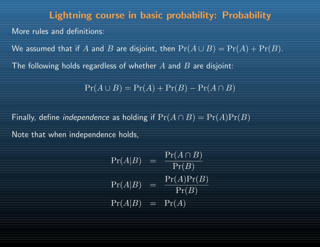
Finally, define independence as holding if Pr(A ∩B) = Pr(A)Pr(B)
Note that when independence holds,
Pr(A|B) =Pr(A ∩B)
Pr(B)
Pr(A|B) =Pr(A)Pr(B)
Pr(B)
Pr(A|B) = Pr(A)
From probability to random variables
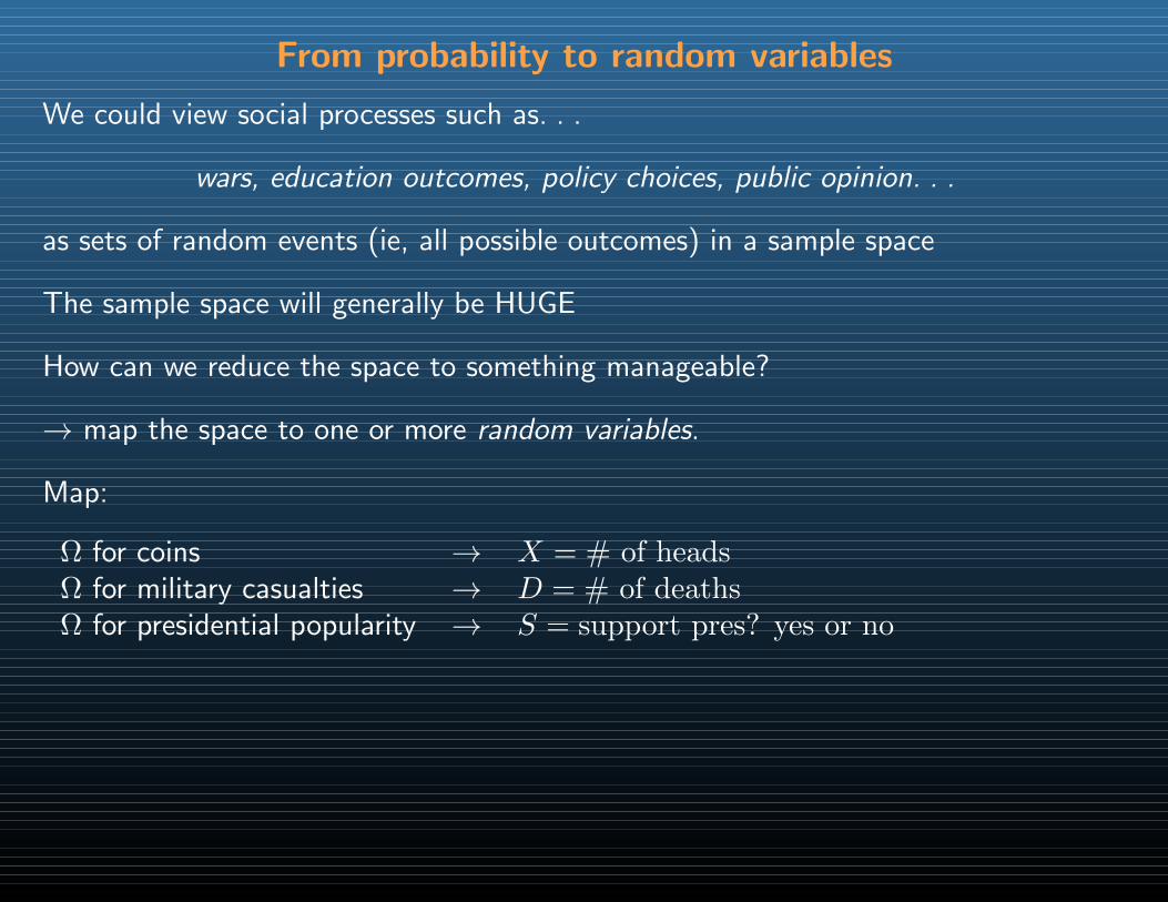
We could view social processes such as. . .
wars, education outcomes, policy choices, public opinion. . .
as sets of random events (ie, all possible outcomes) in a sample space
From probability to random variables
We could view social processes such as. . .
wars, education outcomes, policy choices, public opinion. . .
as sets of random events (ie, all possible outcomes) in a sample space
The sample space will generally be HUGE
From probability to random variables
We could view social processes such as. . .
wars, education outcomes, policy choices, public opinion. . .
as sets of random events (ie, all possible outcomes) in a sample space
The sample space will generally be HUGE
How can we reduce the space to something manageable?
→ map the space to one or more random variables.
Map:
Ω for coins → X = # of heads
From probability to random variables
We could view social processes such as. . .
wars, education outcomes, policy choices, public opinion. . .
as sets of random events (ie, all possible outcomes) in a sample space
The sample space will generally be HUGE
How can we reduce the space to something manageable?
→ map the space to one or more random variables.
Map:
Ω for coins → X = # of headsΩ for military casualties → D = # of deaths
From probability to random variables
We could view social processes such as. . .
wars, education outcomes, policy choices, public opinion. . .
as sets of random events (ie, all possible outcomes) in a sample space
The sample space will generally be HUGE
How can we reduce the space to something manageable?
→ map the space to one or more random variables.
Map:
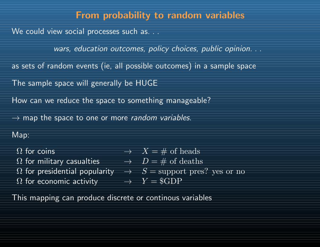
Ω for coins → X = # of headsΩ for military casualties → D = # of deathsΩ for presidential popularity → S = support pres? yes or no
From probability to random variables
We could view social processes such as. . .
wars, education outcomes, policy choices, public opinion. . .
as sets of random events (ie, all possible outcomes) in a sample space
The sample space will generally be HUGE
How can we reduce the space to something manageable?
→ map the space to one or more random variables.
Map:
Ω for coins → X = # of headsΩ for military casualties → D = # of deathsΩ for presidential popularity → S = support pres? yes or noΩ for economic activity → Y = $GDP
This mapping can produce discrete or continous variables
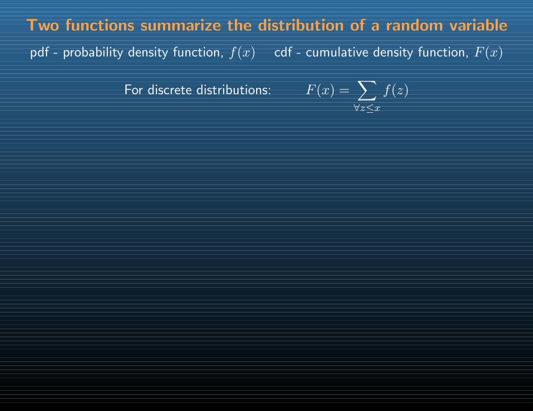
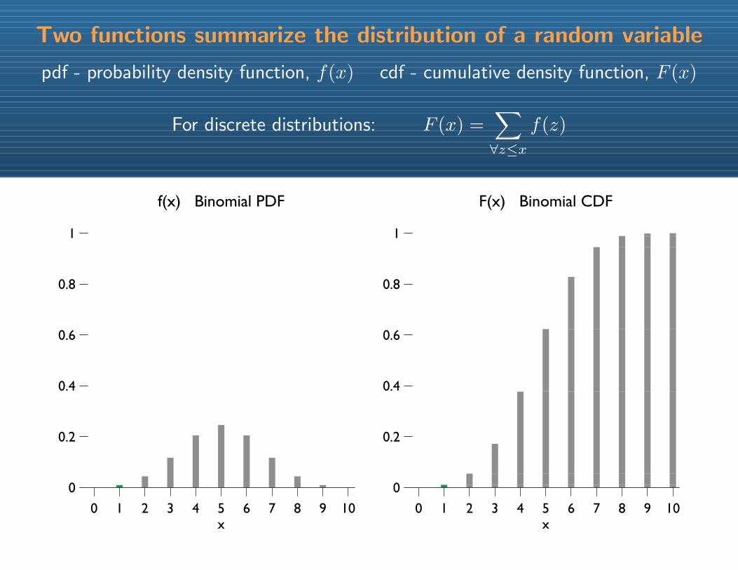
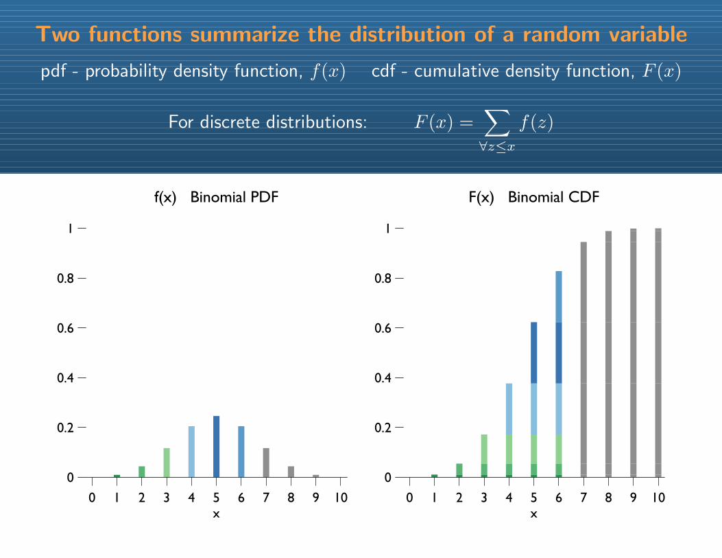
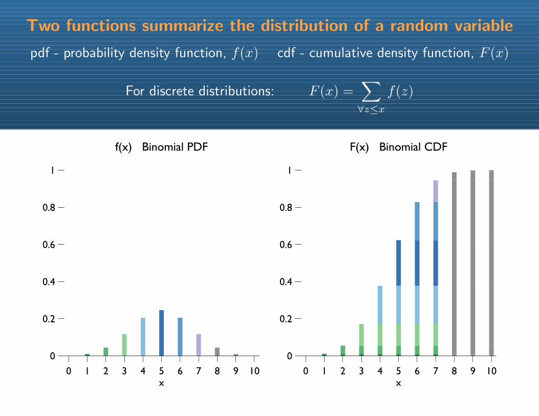
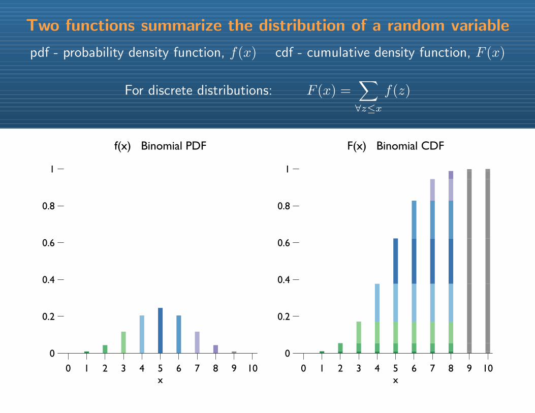
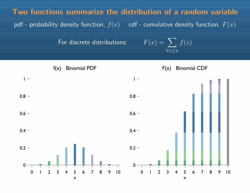
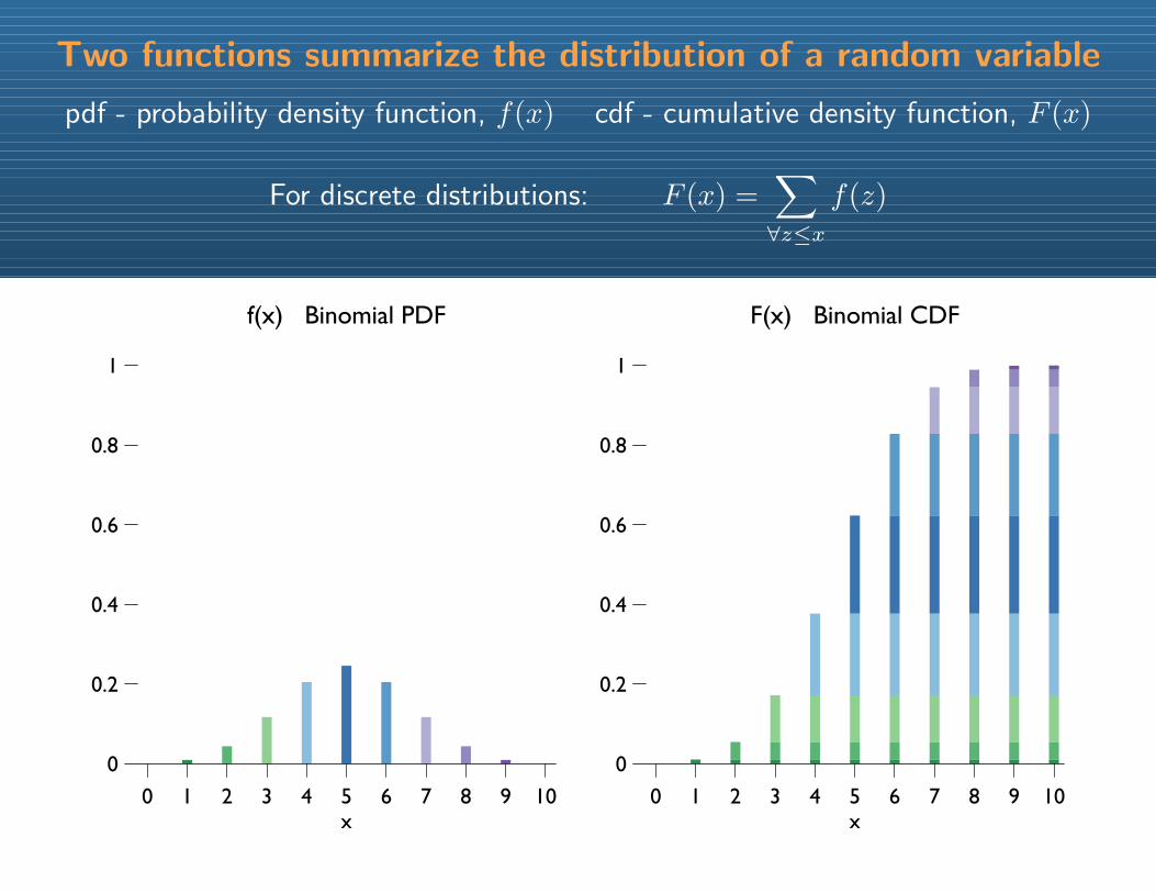
Two functions summarize the distribution of a random variable
pdf - probability density function, f(x) cdf - cumulative density function, F (x)
For discrete distributions: F (x) =∑∀z≤x
f(z)
Two functions summarize the distribution of a random variable
pdf - probability density function, f(x) cdf - cumulative density function, F (x)
For discrete distributions: F (x) =∑∀z≤x
f(z)
0 1 2 3 4 5 6 7 8 9 10
0
0.2
0.4
0.6
0.8
1
f(x) Binomial PDF
x
0 1 2 3 4 5 6 7 8 9 10
0
0.2
0.4
0.6
0.8
1
F(x) Binomial CDF
x
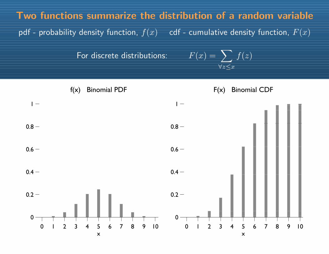
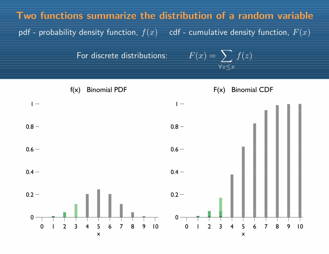
Two functions summarize the distribution of a random variable
pdf - probability density function, f(x) cdf - cumulative density function, F (x)
For discrete distributions: F (x) =∑∀z≤x
f(z)
0 1 2 3 4 5 6 7 8 9 10
0
0.2
0.4
0.6
0.8
1
f(x) Binomial PDF
x0 1 2 3 4 5 6 7 8 9 10
0
0.2
0.4
0.6
0.8
1
F(x) Binomial CDF
x
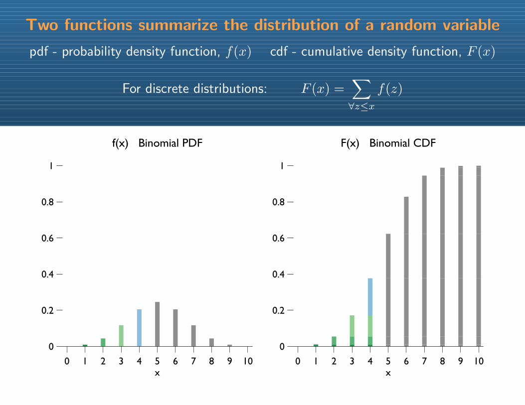
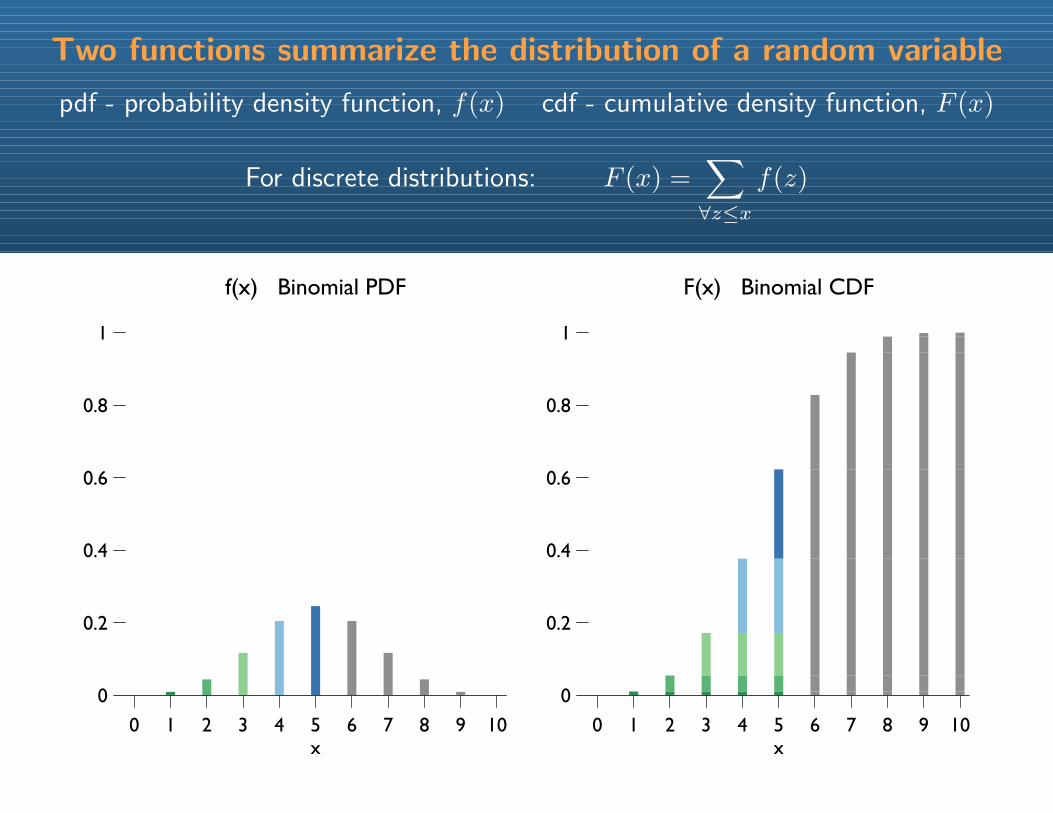
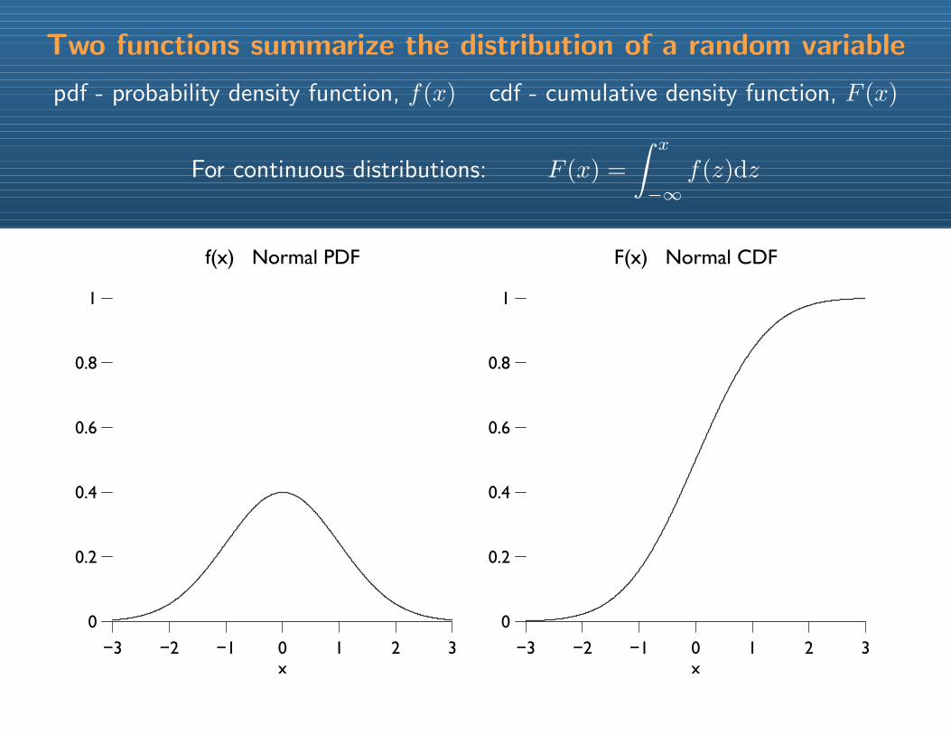
Two functions summarize the distribution of a random variable
pdf - probability density function, f(x) cdf - cumulative density function, F (x)
For continuous distributions: F (x) =
∫ x
−∞f(z)dz
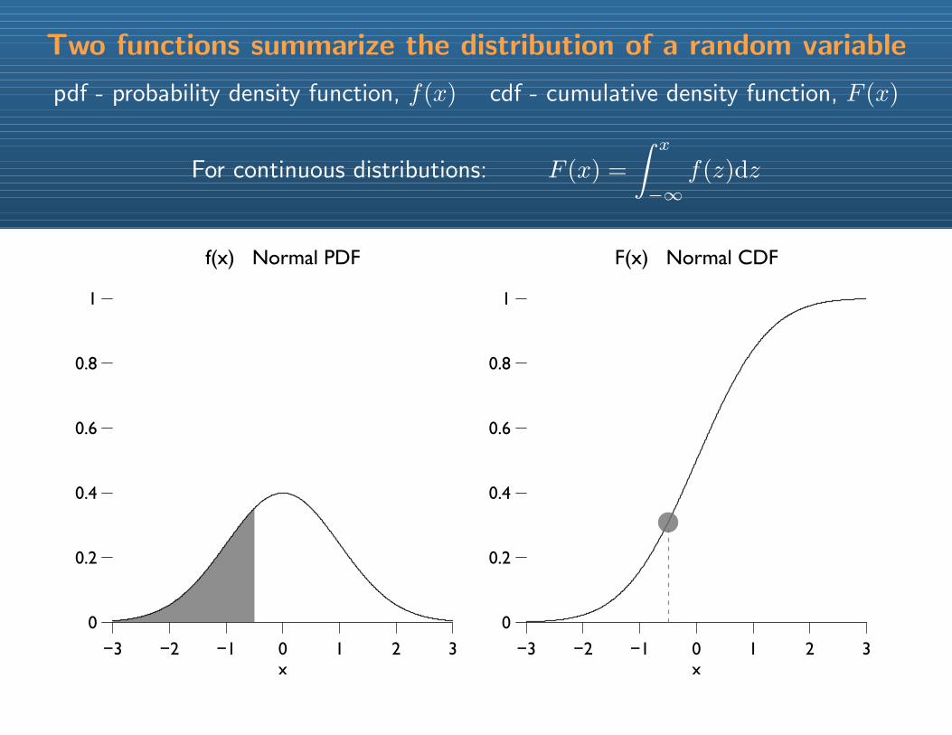
Two functions summarize the distribution of a random variable
pdf - probability density function, f(x) cdf - cumulative density function, F (x)
For continuous distributions: F (x) =
∫ x
−∞f(z)dz
−3 −2 −1 0 1 2 3
0
0.2
0.4
0.6
0.8
1
f(x) Normal PDF
x−3 −2 −1 0 1 2 3
0
0.2
0.4
0.6
0.8
1
F(x) Normal CDF
x
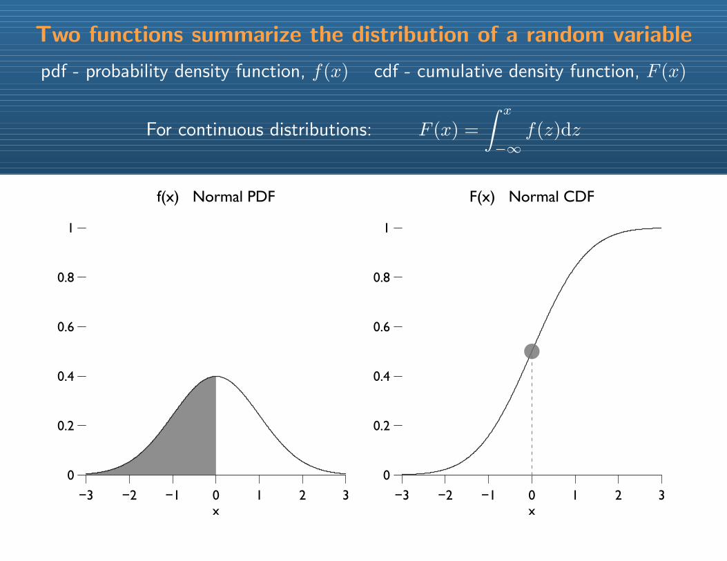
Two functions summarize the distribution of a random variable
pdf - probability density function, f(x) cdf - cumulative density function, F (x)
For continuous distributions: F (x) =
∫ x
−∞f(z)dz
−3 −2 −1 0 1 2 3
0
0.2
0.4
0.6
0.8
1
f(x) Normal PDF
x−3 −2 −1 0 1 2 3
0
0.2
0.4
0.6
0.8
1
F(x) Normal CDF
x
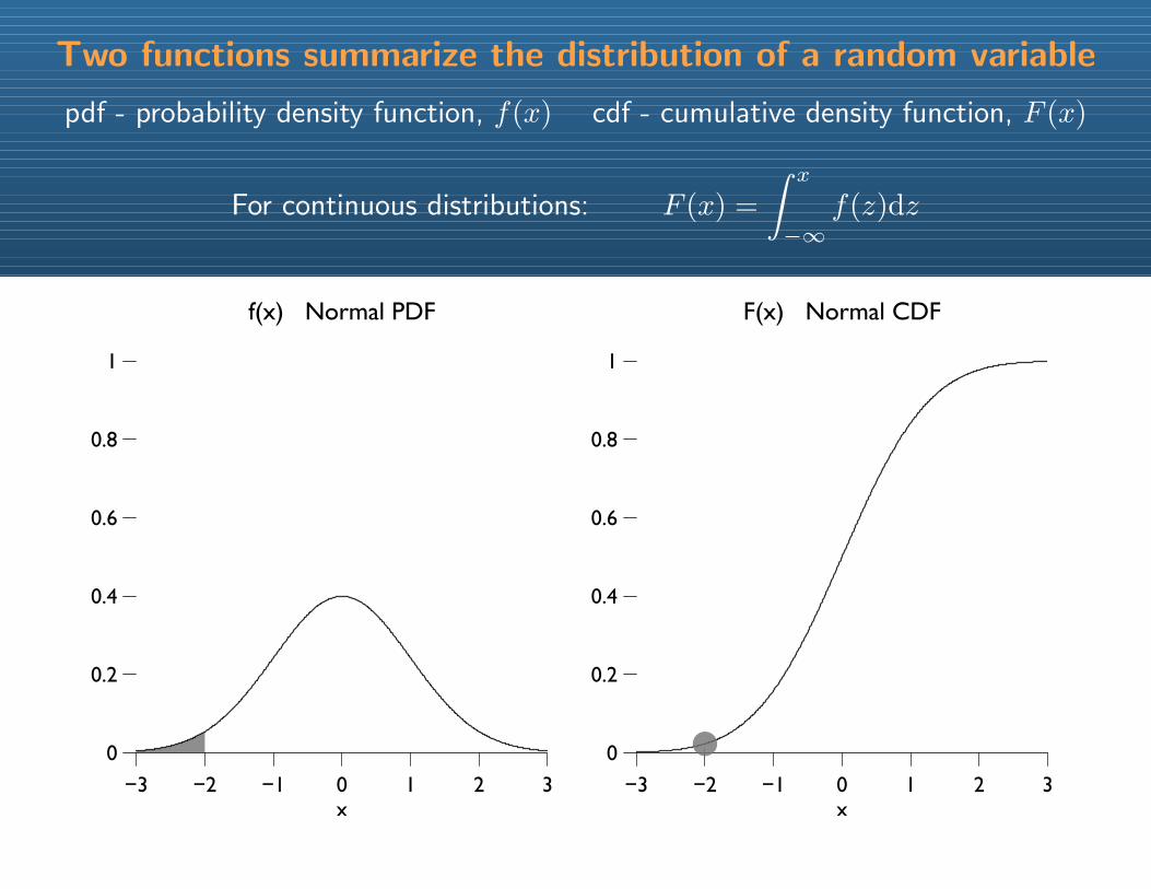
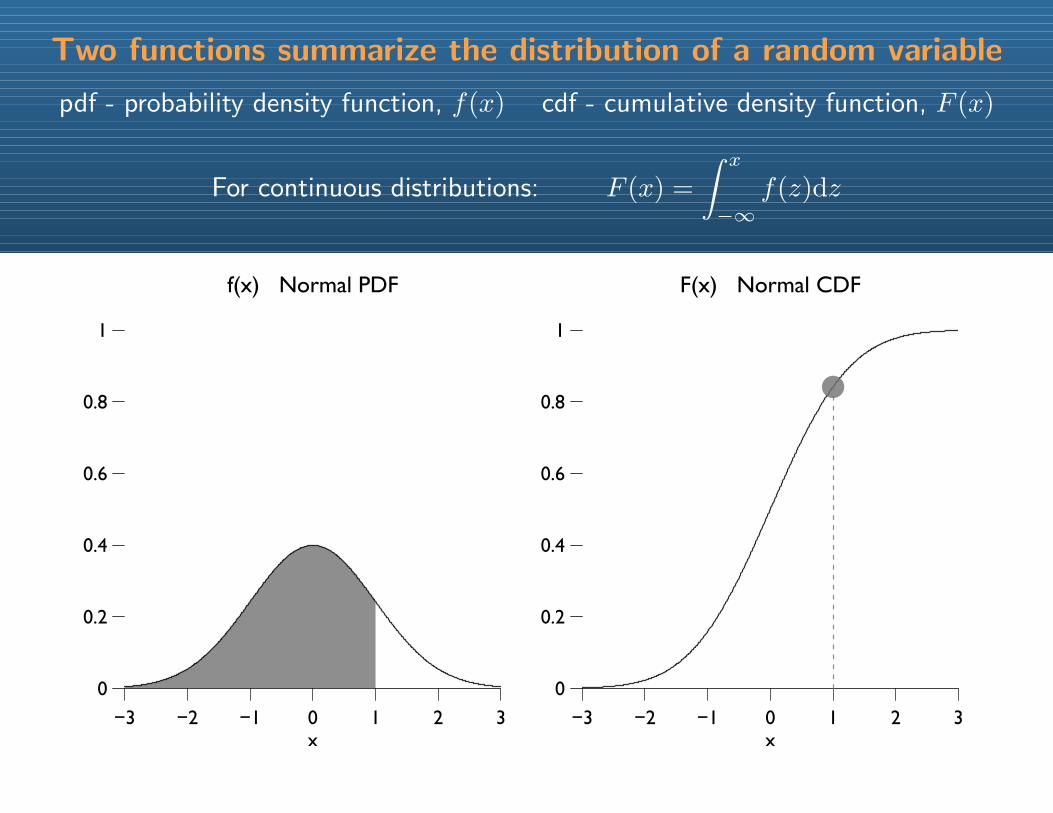
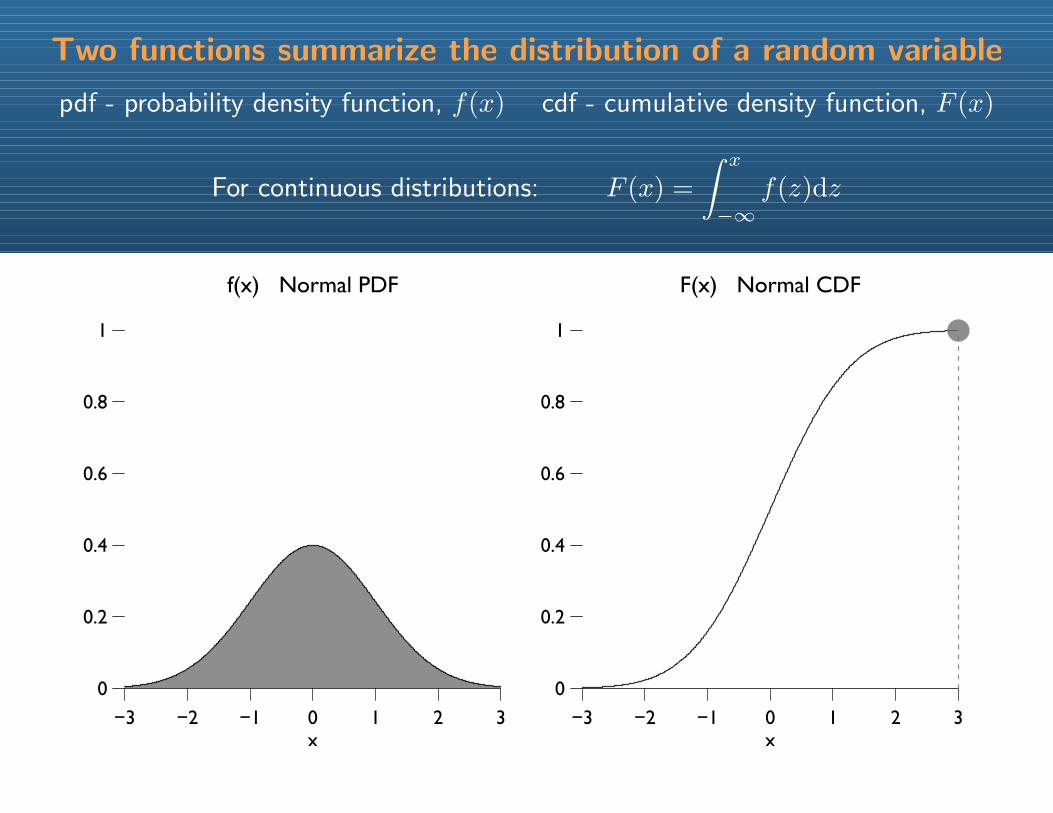
Example probability distributions
1000s of probability distributions are described in the statistical literature
Example probability distributions
1000s of probability distributions are described in the statistical literature
They are mathematical descriptions of RVs based on different assumptions
Example probability distributions
1000s of probability distributions are described in the statistical literature
They are mathematical descriptions of RVs based on different assumptions
Choose a probability distribution with assumptions thatmatch the substance of the social process under study
Example probability distributions
1000s of probability distributions are described in the statistical literature
They are mathematical descriptions of RVs based on different assumptions
Choose a probability distribution with assumptions thatmatch the substance of the social process under study
Let’s look at a few distributions to see how this might work
Bear in mind the key distinction between continuous and discrete distributions
Let’s start with the simplest and most fundamental discrete distribution,the Bernoulli
The Bernoulli distribution
Consider a random variable x with 2 mutually exclusive & exhaustive outcomes
The Bernoulli distribution
Consider a random variable x with 2 mutually exclusive & exhaustive outcomes
Let there be one parameter, the probability of “success,” labelled π
The Bernoulli distribution
Consider a random variable x with 2 mutually exclusive & exhaustive outcomes
Let there be one parameter, the probability of “success,” labelled π
Without loss of generality, let x ∈ 0, 1 where 1 = success

The Bernoulli distribution
Consider a random variable x with 2 mutually exclusive & exhaustive outcomes
Let there be one parameter, the probability of “success,” labelled π
Without loss of generality, let x ∈ 0, 1 where 1 = success
These assumptions create the Bernoulli distribution (pdf and cdf below):
0tails
1heads
Pr(outcome)Bernoulli pdf
11
0tails
1heads
Bernoulli cdf
x x
π
π1–
π
π1–
The Bernoulli distribution
Consider a random variable x with 2 mutually exclusive & exhaustive outcomes
Let there be one parameter, the probability of “success,” labelled π
Without loss of generality, let x ∈ 0, 1 where 1 = success
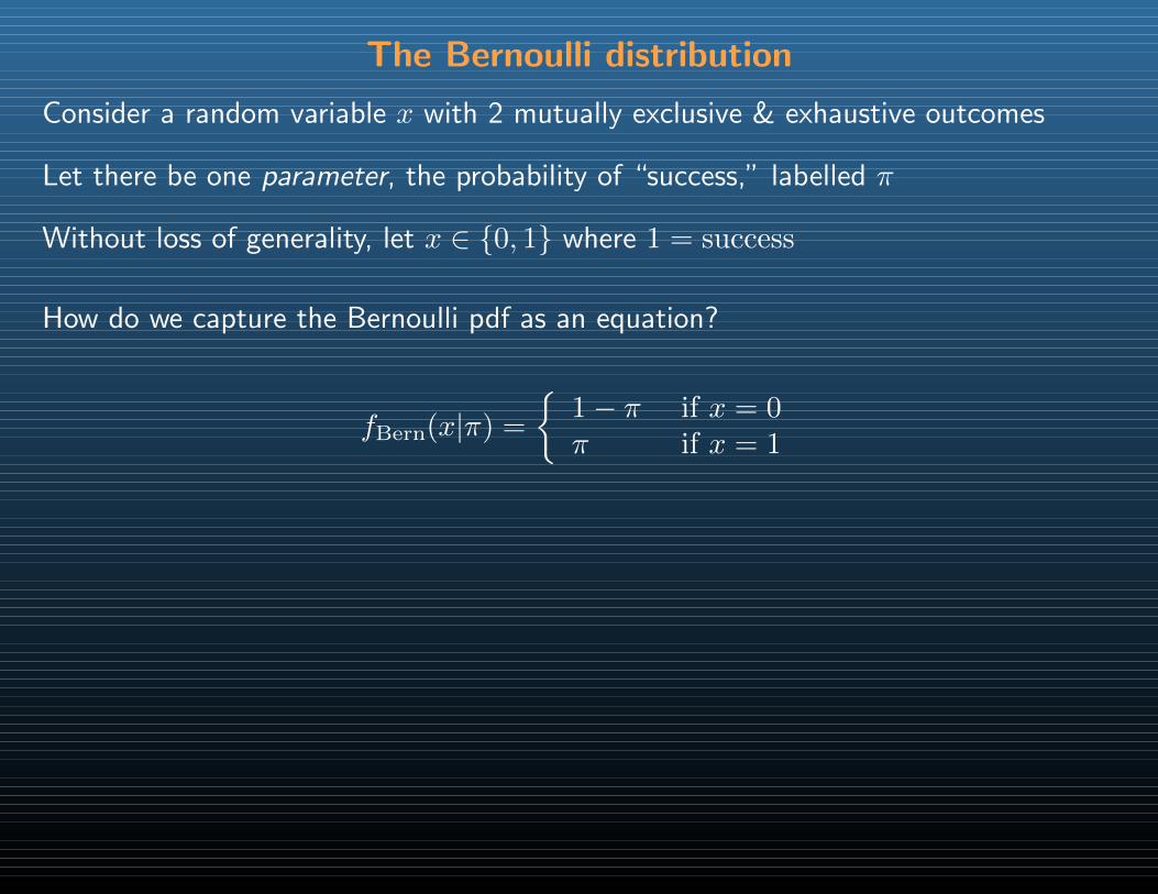
How do we capture the Bernoulli pdf as an equation?
The Bernoulli distribution
Consider a random variable x with 2 mutually exclusive & exhaustive outcomes
Let there be one parameter, the probability of “success,” labelled π
Without loss of generality, let x ∈ 0, 1 where 1 = success
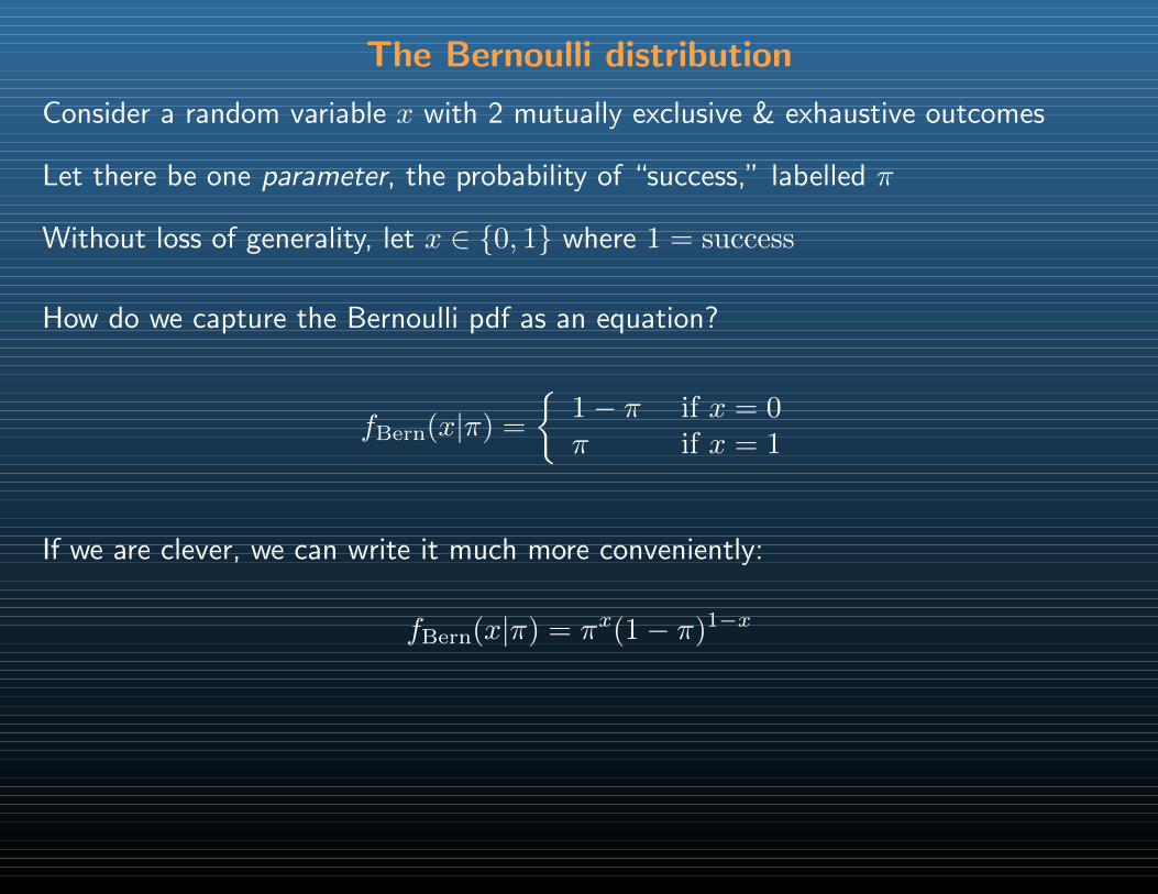
How do we capture the Bernoulli pdf as an equation?
fBern(x|π) =
1− π if x = 0π if x = 1
The Bernoulli distribution
Consider a random variable x with 2 mutually exclusive & exhaustive outcomes
Let there be one parameter, the probability of “success,” labelled π
Without loss of generality, let x ∈ 0, 1 where 1 = success
How do we capture the Bernoulli pdf as an equation?
fBern(x|π) =
1− π if x = 0π if x = 1
If we are clever, we can write it much more conveniently:
fBern(x|π) = πx(1− π)1−x
The Bernoulli distribution
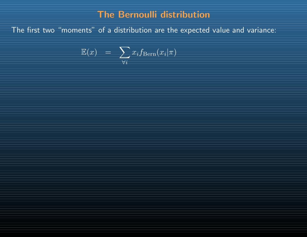
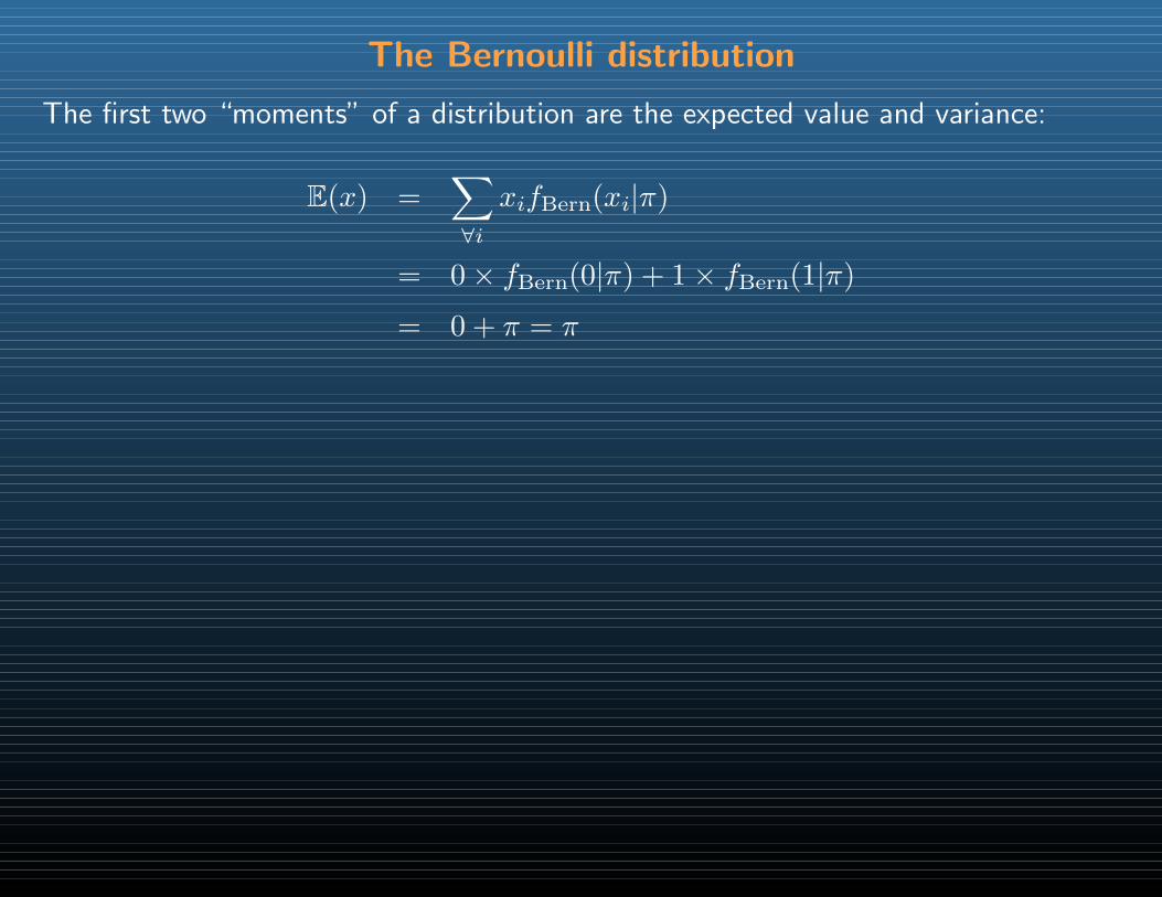
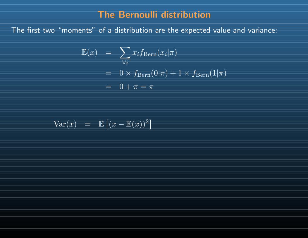
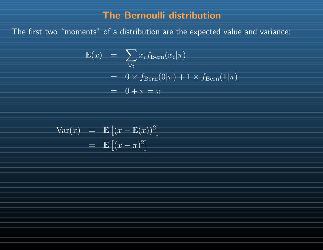
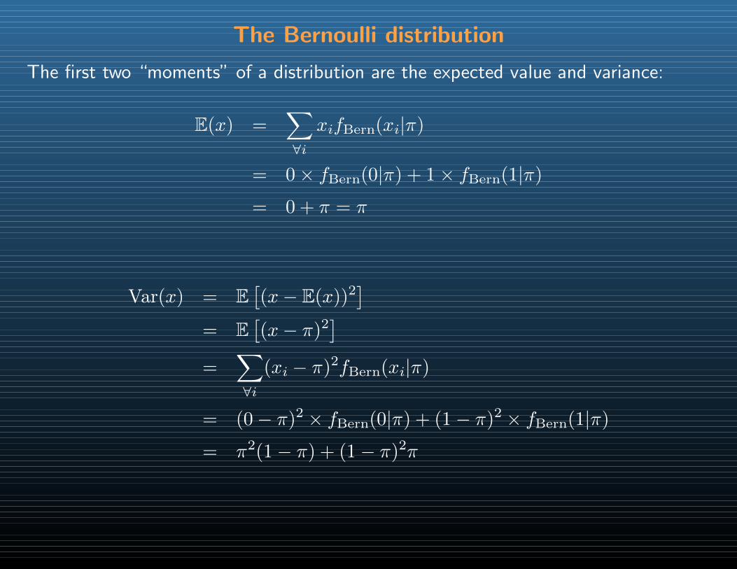
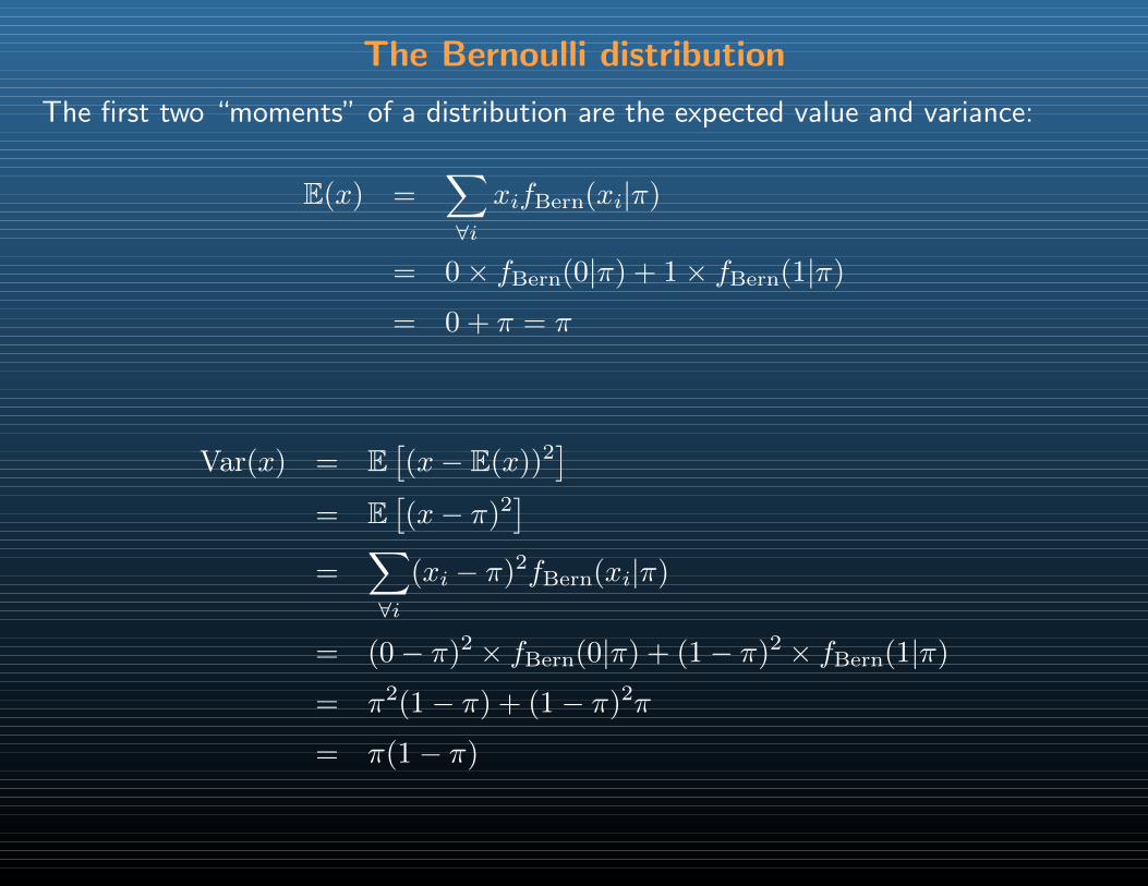
The first two “moments” of a distribution are the expected value and variance:
E(x) =∑∀i
xifBern(xi|π)

The Bernoulli distribution
The first two “moments” of a distribution are the expected value and variance:
E(x) =∑∀i
xifBern(xi|π)
= 0× fBern(0|π) + 1× fBern(1|π)
The Bernoulli distribution
The first two “moments” of a distribution are the expected value and variance:
E(x) =∑∀i
xifBern(xi|π)
= 0× fBern(0|π) + 1× fBern(1|π)
= 0 + π = π
The Bernoulli distribution
The first two “moments” of a distribution are the expected value and variance:
E(x) =∑∀i
xifBern(xi|π)
= 0× fBern(0|π) + 1× fBern(1|π)
= 0 + π = π
Var(x) = E[(x− E(x))2
]
The Bernoulli distribution
The first two “moments” of a distribution are the expected value and variance:
E(x) =∑∀i
xifBern(xi|π)
= 0× fBern(0|π) + 1× fBern(1|π)
= 0 + π = π
Var(x) = E[(x− E(x))2
]= E
[(x− π)2
]
The Bernoulli distribution
The first two “moments” of a distribution are the expected value and variance:
E(x) =∑∀i
xifBern(xi|π)
= 0× fBern(0|π) + 1× fBern(1|π)
= 0 + π = π
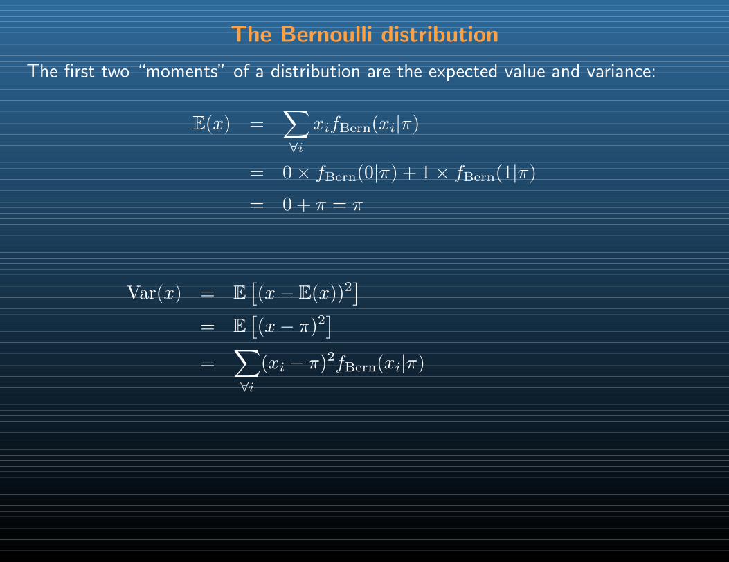
Var(x) = E[(x− E(x))2
]= E
[(x− π)2
]=
∑∀i
(xi − π)2fBern(xi|π)
The Bernoulli distribution
The first two “moments” of a distribution are the expected value and variance:
E(x) =∑∀i
xifBern(xi|π)
= 0× fBern(0|π) + 1× fBern(1|π)
= 0 + π = π
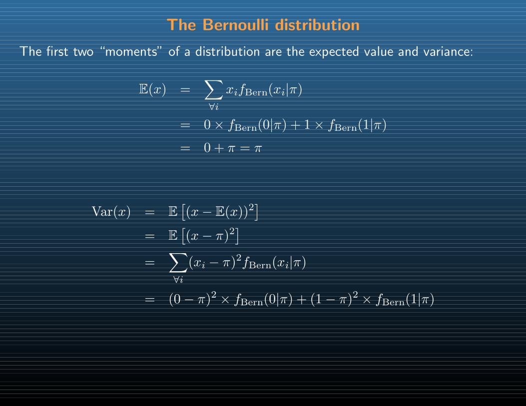
Var(x) = E[(x− E(x))2
]= E
[(x− π)2
]=
∑∀i
(xi − π)2fBern(xi|π)
= (0− π)2 × fBern(0|π) + (1− π)2 × fBern(1|π)
The Bernoulli distribution
The first two “moments” of a distribution are the expected value and variance:
E(x) =∑∀i
xifBern(xi|π)
= 0× fBern(0|π) + 1× fBern(1|π)
= 0 + π = π
Var(x) = E[(x− E(x))2
]= E
[(x− π)2
]=
∑∀i
(xi − π)2fBern(xi|π)
= (0− π)2 × fBern(0|π) + (1− π)2 × fBern(1|π)
= π2(1− π) + (1− π)2π
= π(1− π)
The binomial distribution
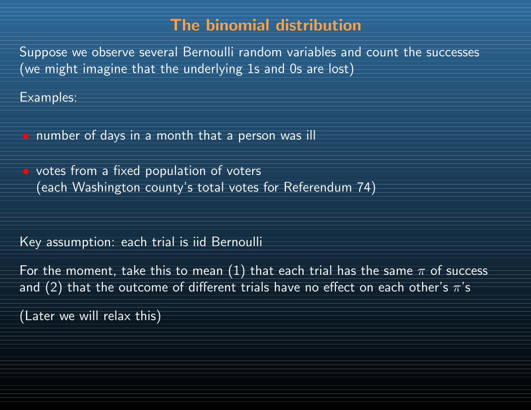
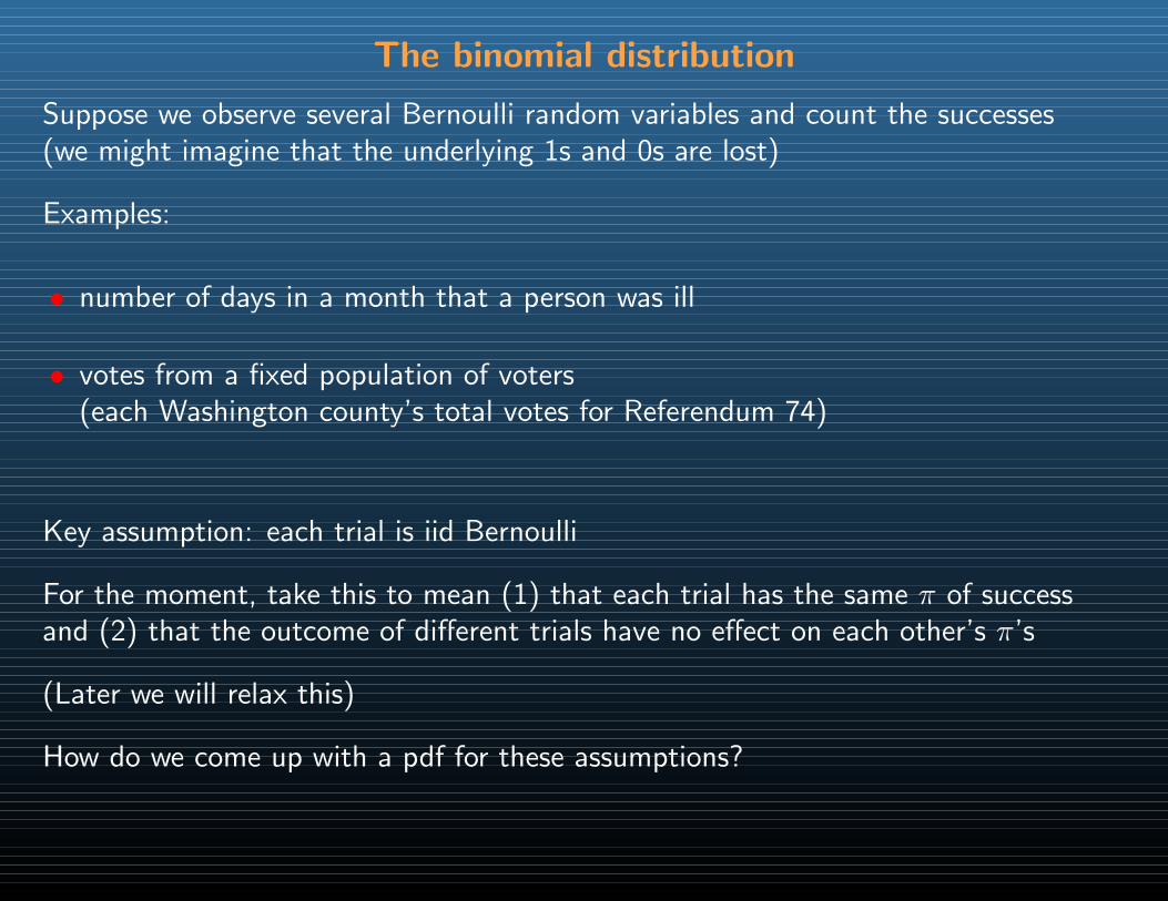
Suppose we observe several Bernoulli random variables and count the successes(we might imagine that the underlying 1s and 0s are lost)
The binomial distribution
Suppose we observe several Bernoulli random variables and count the successes(we might imagine that the underlying 1s and 0s are lost)
Examples:
• number of days in a month that a person was ill
• votes from a fixed population of voters(each Washington county’s total votes for Referendum 74)
Key assumption: each trial is iid Bernoulli
For the moment, take this to mean (1) that each trial has the same π of successand (2) that the outcome of different trials have no effect on each other’s π’s
(Later we will relax this)
How do we come up with a pdf for these assumptions?
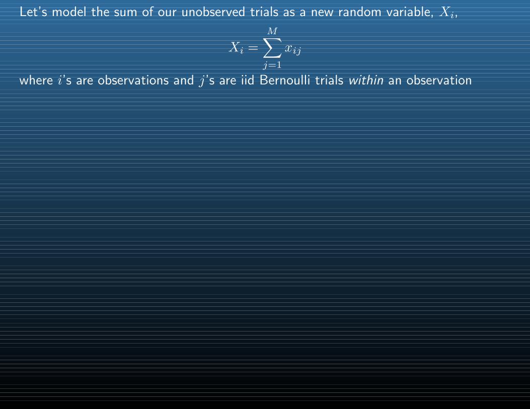
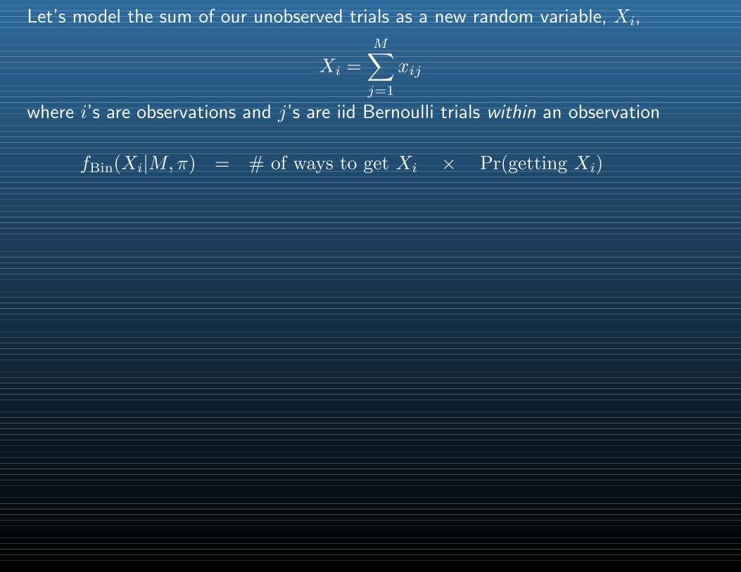
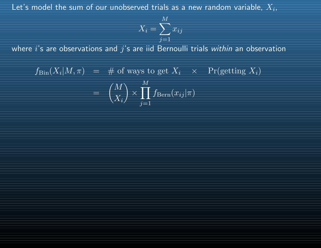
Let’s model the sum of our unobserved trials as a new random variable, Xi,
Xi =
M∑j=1
xij
where i’s are observations and j’s are iid Bernoulli trials within an observation
Let’s model the sum of our unobserved trials as a new random variable, Xi,
Xi =
M∑j=1
xij
where i’s are observations and j’s are iid Bernoulli trials within an observation
fBin(Xi|M,π) = # of ways to get Xi × Pr(getting Xi)
Let’s model the sum of our unobserved trials as a new random variable, Xi,
Xi =
M∑j=1
xij
where i’s are observations and j’s are iid Bernoulli trials within an observation
fBin(Xi|M,π) = # of ways to get Xi × Pr(getting Xi)
=
(M
Xi
)×
M∏j=1
fBern(xij|π)
Let’s model the sum of our unobserved trials as a new random variable, Xi,
Xi =
M∑j=1
xij
where i’s are observations and j’s are iid Bernoulli trials within an observation
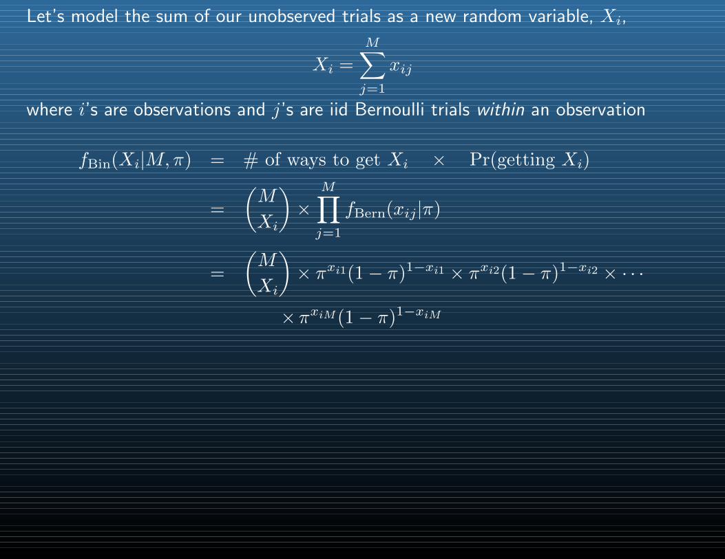
fBin(Xi|M,π) = # of ways to get Xi × Pr(getting Xi)
=
(M
Xi
)×
M∏j=1
fBern(xij|π)
=
(M
Xi
)× πxi1(1− π)1−xi1 × πxi2(1− π)1−xi2 × · · ·
×πxiM(1− π)1−xiM
Let’s model the sum of our unobserved trials as a new random variable, Xi,
Xi =
M∑j=1
xij
where i’s are observations and j’s are iid Bernoulli trials within an observation
fBin(Xi|M,π) = # of ways to get Xi × Pr(getting Xi)
=
(M
Xi
)×
M∏j=1
fBern(xij|π)
=
(M
Xi
)× πxi1(1− π)1−xi1 × πxi2(1− π)1−xi2 × · · ·
×πxiM(1− π)1−xiM
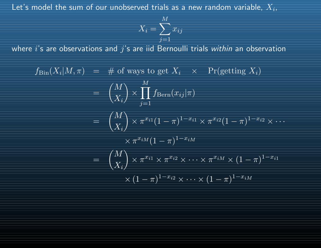
=
(M
Xi
)× πxi1 × πxi2 × · · · × πxiM × (1− π)1−xi1
× (1− π)1−xi2 × · · · × (1− π)1−xiM
Let’s model the sum of our unobserved trials as a new random variable, Xi,
Xi =
M∑j=1
xij
where i’s are observations and j’s are iid Bernoulli trials within an observation
fBin(Xi|M,π) = # of ways to get Xi × Pr(getting Xi)
=
(M
Xi
)×
M∏j=1
fBern(xij|π)
=
(M
Xi
)× πxi1(1− π)1−xi1 × πxi2(1− π)1−xi2 × · · ·
×πxiM(1− π)1−xiM
=
(M
Xi
)× πxi1 × πxi2 × · · · × πxiM × (1− π)1−xi1
× (1− π)1−xi2 × · · · × (1− π)1−xiM
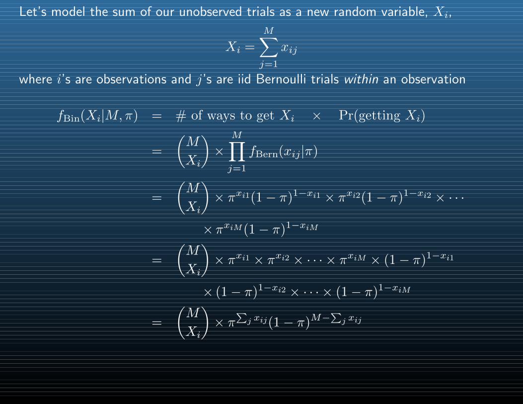
=
(M
Xi
)× π
∑j xij(1− π)M−
∑j xij

Let’s model the sum of our unobserved trials as a new random variable, Xi,
Xi =
M∑j=1
xij
where i’s are observations and j’s are iid Bernoulli trials within an observation
fBin(Xi|M,π) = # of ways to get Xi × Pr(getting Xi)
=
(M
Xi
)×
M∏j=1
fBern(xij|π)
=
(M
Xi
)× πxi1(1− π)1−xi1 × πxi2(1− π)1−xi2 × · · ·
×πxiM(1− π)1−xiM
=
(M
Xi
)× πxi1 × πxi2 × · · · × πxiM × (1− π)1−xi1
× (1− π)1−xi2 × · · · × (1− π)1−xiM
=
(M
Xi
)× π
∑j xij(1− π)M−
∑j xij
=M !
Xi!(M −Xi)!πXi(1− π)M−Xi
The binomial distribution
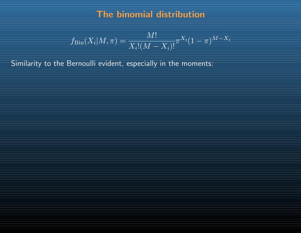
fBin(Xi|M,π) =M !
Xi!(M −Xi)!πXi(1− π)M−Xi
Similarity to the Bernoulli evident, especially in the moments:
The binomial distribution
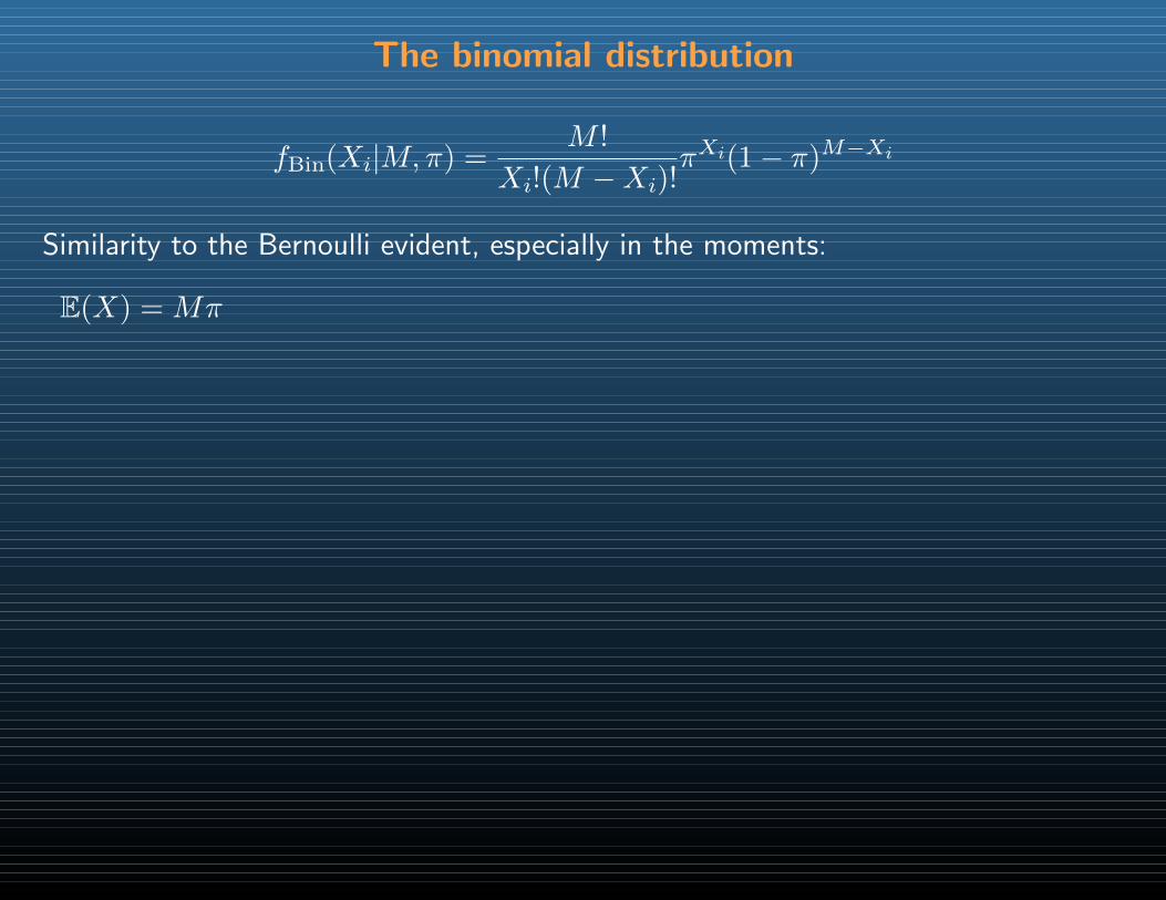
fBin(Xi|M,π) =M !
Xi!(M −Xi)!πXi(1− π)M−Xi
Similarity to the Bernoulli evident, especially in the moments:
E(X) = Mπ
The binomial distribution
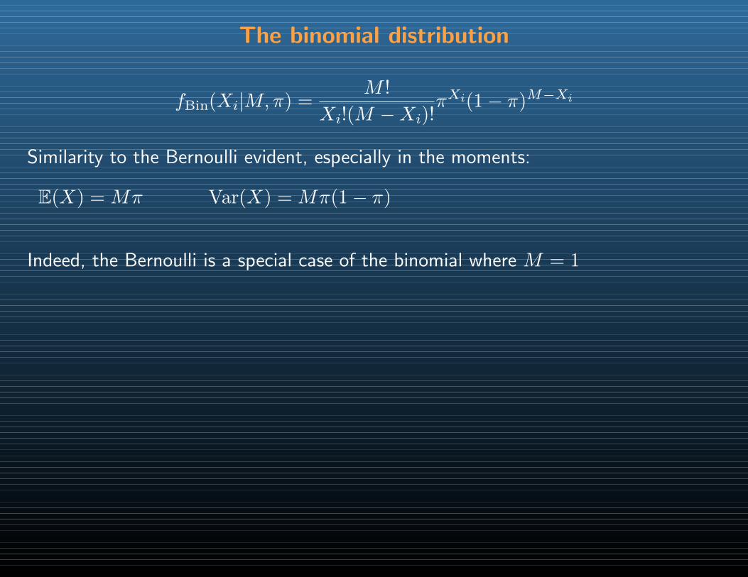
fBin(Xi|M,π) =M !
Xi!(M −Xi)!πXi(1− π)M−Xi
Similarity to the Bernoulli evident, especially in the moments:
E(X) = Mπ Var(X) = Mπ(1− π)
Indeed, the Bernoulli is a special case of the binomial where M = 1
The binomial distribution
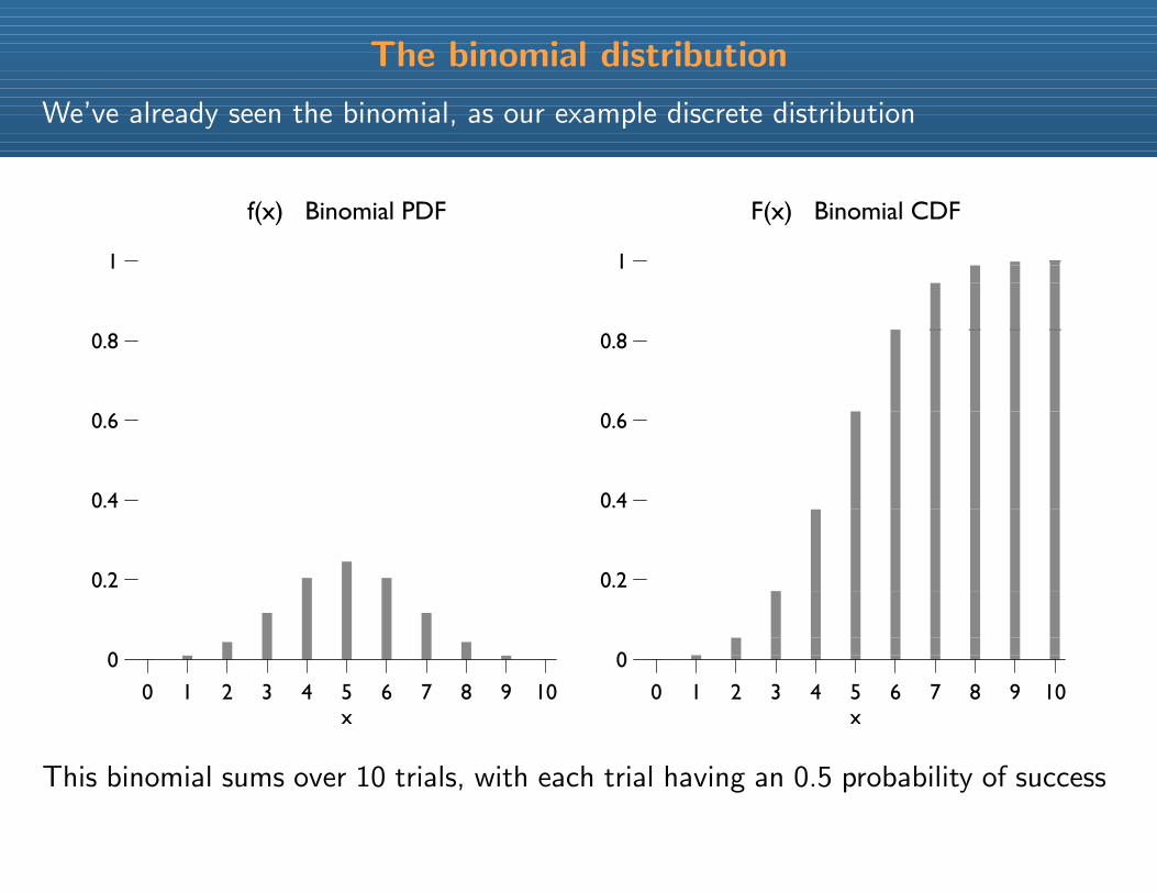
We’ve already seen the binomial, as our example discrete distribution
0 1 2 3 4 5 6 7 8 9 10
0
0.2
0.4
0.6
0.8
1
f(x) Binomial PDF
x
0 1 2 3 4 5 6 7 8 9 10
0
0.2
0.4
0.6
0.8
1
F(x) Binomial CDF
x
This binomial sums over 10 trials, with each trial having an 0.5 probability of success
The Poisson distribution
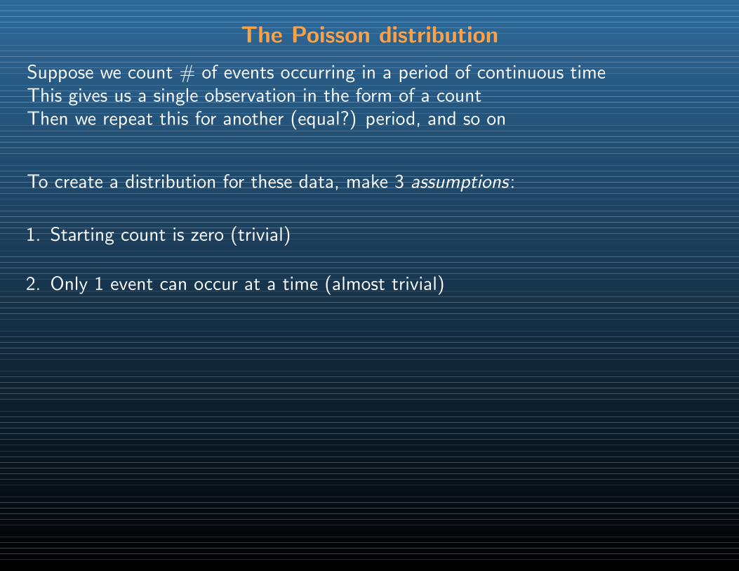
Suppose we count # of events occurring in a period of continuous time
The Poisson distribution
Suppose we count # of events occurring in a period of continuous timeThis gives us a single observation in the form of a count
The Poisson distribution
Suppose we count # of events occurring in a period of continuous timeThis gives us a single observation in the form of a countThen we repeat this for another (equal?) period, and so on
The Poisson distribution
Suppose we count # of events occurring in a period of continuous timeThis gives us a single observation in the form of a countThen we repeat this for another (equal?) period, and so on
To create a distribution for these data, make 3 assumptions:
1. Starting count is zero (trivial)
2. Only 1 event can occur at a time (almost trivial)
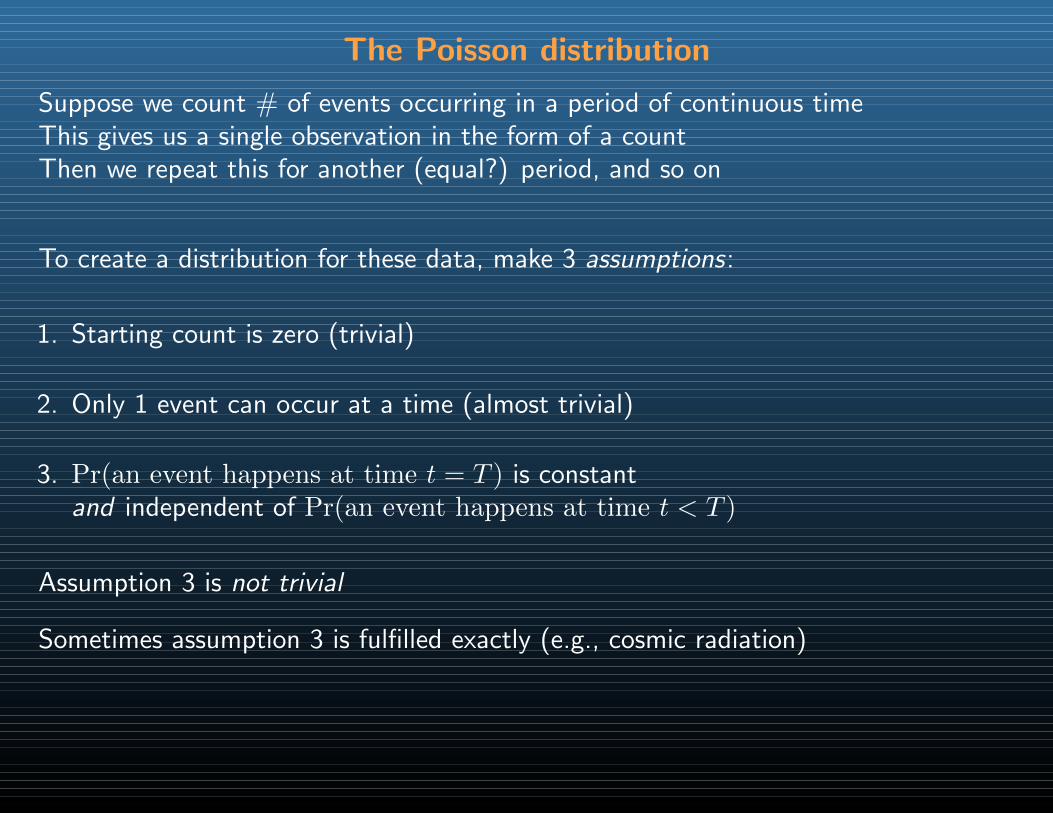
3. Pr(an event happens at time t = T ) is constantand independent of Pr(an event happens at time t < T )
The Poisson distribution
Suppose we count # of events occurring in a period of continuous timeThis gives us a single observation in the form of a countThen we repeat this for another (equal?) period, and so on
To create a distribution for these data, make 3 assumptions:
1. Starting count is zero (trivial)
2. Only 1 event can occur at a time (almost trivial)
3. Pr(an event happens at time t = T ) is constantand independent of Pr(an event happens at time t < T )
Assumption 3 is not trivial
Sometimes assumption 3 is fulfilled exactly (e.g., cosmic radiation)
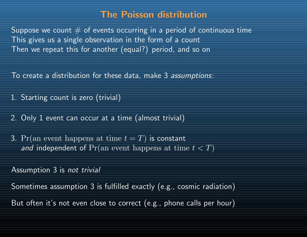
But often it’s not even close to correct (e.g., phone calls per hour)
The Poisson distribution
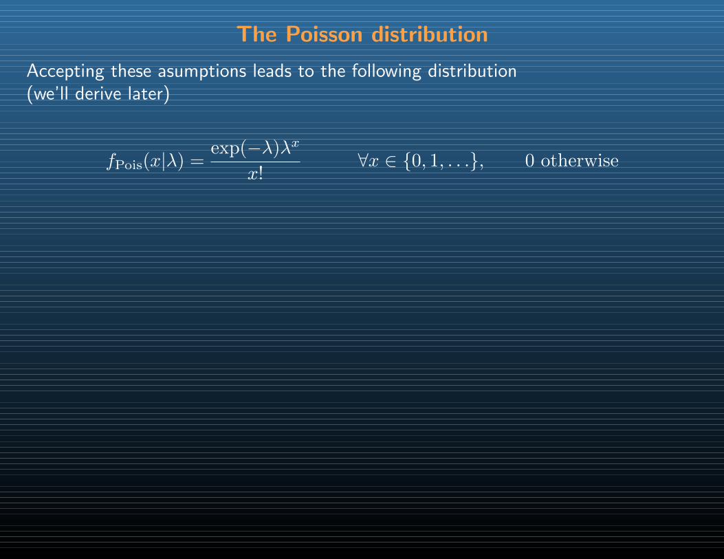
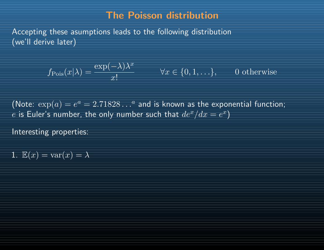
Accepting these asumptions leads to the following distribution(we’ll derive later)
fPois(x|λ) =exp(−λ)λx
x!∀x ∈ 0, 1, . . ., 0 otherwise
The Poisson distribution
Accepting these asumptions leads to the following distribution(we’ll derive later)
fPois(x|λ) =exp(−λ)λx
x!∀x ∈ 0, 1, . . ., 0 otherwise
(Note: exp(a) = ea = 2.71828 . . .a and is known as the exponential function;e is Euler’s number, the only number such that dex/dx = ex)
Interesting properties:
1. E(x) = var(x) = λ
The Poisson distribution
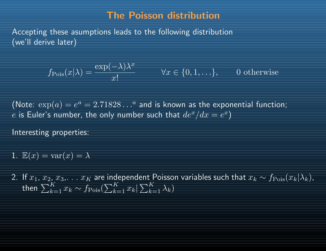
Accepting these asumptions leads to the following distribution(we’ll derive later)
fPois(x|λ) =exp(−λ)λx
x!∀x ∈ 0, 1, . . ., 0 otherwise
(Note: exp(a) = ea = 2.71828 . . .a and is known as the exponential function;e is Euler’s number, the only number such that dex/dx = ex)
Interesting properties:
1. E(x) = var(x) = λ
2. If x1, x2, x3,. . . xK are independent Poisson variables such that xk ∼ fPois(xk|λk),
then∑Kk=1 xk ∼ fPois(
∑Kk=1 xk|
∑Kk=1 λk)
The Poisson distribution
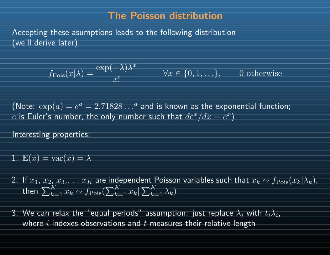
Accepting these asumptions leads to the following distribution(we’ll derive later)
fPois(x|λ) =exp(−λ)λx
x!∀x ∈ 0, 1, . . ., 0 otherwise
(Note: exp(a) = ea = 2.71828 . . .a and is known as the exponential function;e is Euler’s number, the only number such that dex/dx = ex)
Interesting properties:
1. E(x) = var(x) = λ
2. If x1, x2, x3,. . . xK are independent Poisson variables such that xk ∼ fPois(xk|λk),
then∑Kk=1 xk ∼ fPois(
∑Kk=1 xk|
∑Kk=1 λk)
3. We can relax the “equal periods” assumption: just replace λi with tiλi,where i indexes observations and t measures their relative length
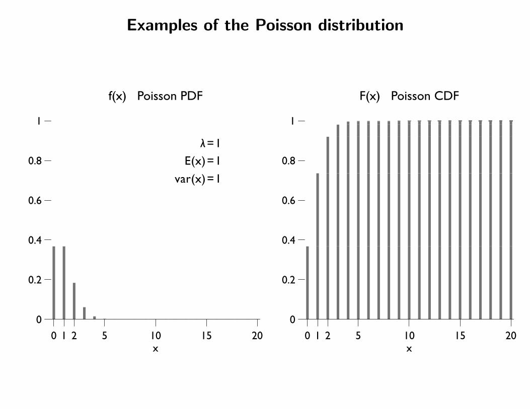
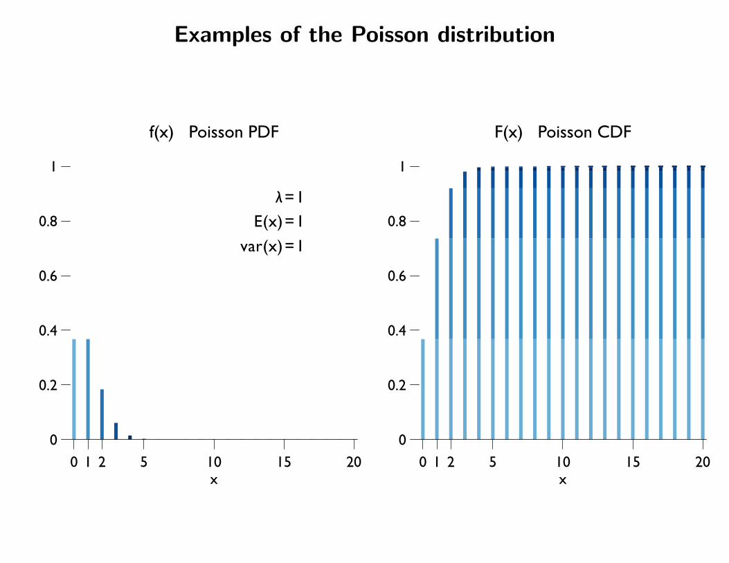
Examples of the Poisson distribution
0 1 2 5 10 15 20
0
0.2
0.4
0.6
0.8
1
f(x) Poisson PDF
x0 1 2 5 10 15 20
0
0.2
0.4
0.6
0.8
1
F(x) Poisson CDF
x
λ=1E(x)=1
var(x)=1
Examples of the Poisson distribution
0 1 2 5 10 15 20
0
0.2
0.4
0.6
0.8
1
f(x) Poisson PDF
x0 1 2 5 10 15 20
0
0.2
0.4
0.6
0.8
1
F(x) Poisson CDF
x
λ=1E(x)=1
var(x)=1

Examples of the Poisson distribution
0 1 2 5 10 15 20
0
0.2
0.4
0.6
0.8
1
f(x) Poisson PDF
x0 1 2 5 10 15 20
0
0.2
0.4
0.6
0.8
1
F(x) Poisson CDF
x
λ=1E(x)=1
var(x)=1
Examples of the Poisson distribution
0 1 2 5 10 15 20
0
0.2
0.4
0.6
0.8
1
f(x) Poisson PDF
x0 1 2 5 10 15 20
0
0.2
0.4
0.6
0.8
1
F(x) Poisson CDF
x
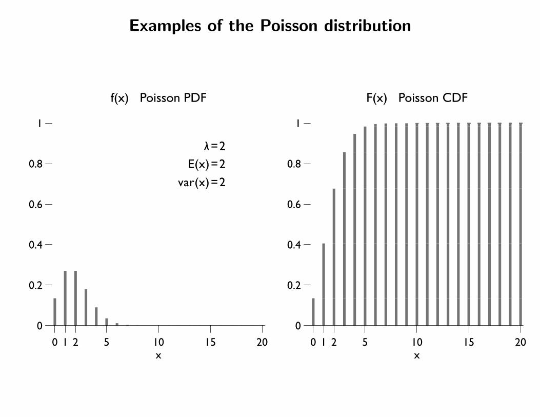
λ=2E(x)=2
var(x)=2
Examples of the Poisson distribution
0 1 2 5 10 15 20
0
0.2
0.4
0.6
0.8
1
f(x) Poisson PDF
x0 1 2 5 10 15 20
0
0.2
0.4
0.6
0.8
1
F(x) Poisson CDF
x
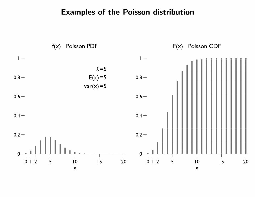
λ=5E(x)=5
var(x)=5
Examples of the Poisson distribution
0 1 2 5 10 15 20
0
0.2
0.4
0.6
0.8
1
f(x) Poisson PDF
x0 1 2 5 10 15 20
0
0.2
0.4
0.6
0.8
1
F(x) Poisson CDF
x
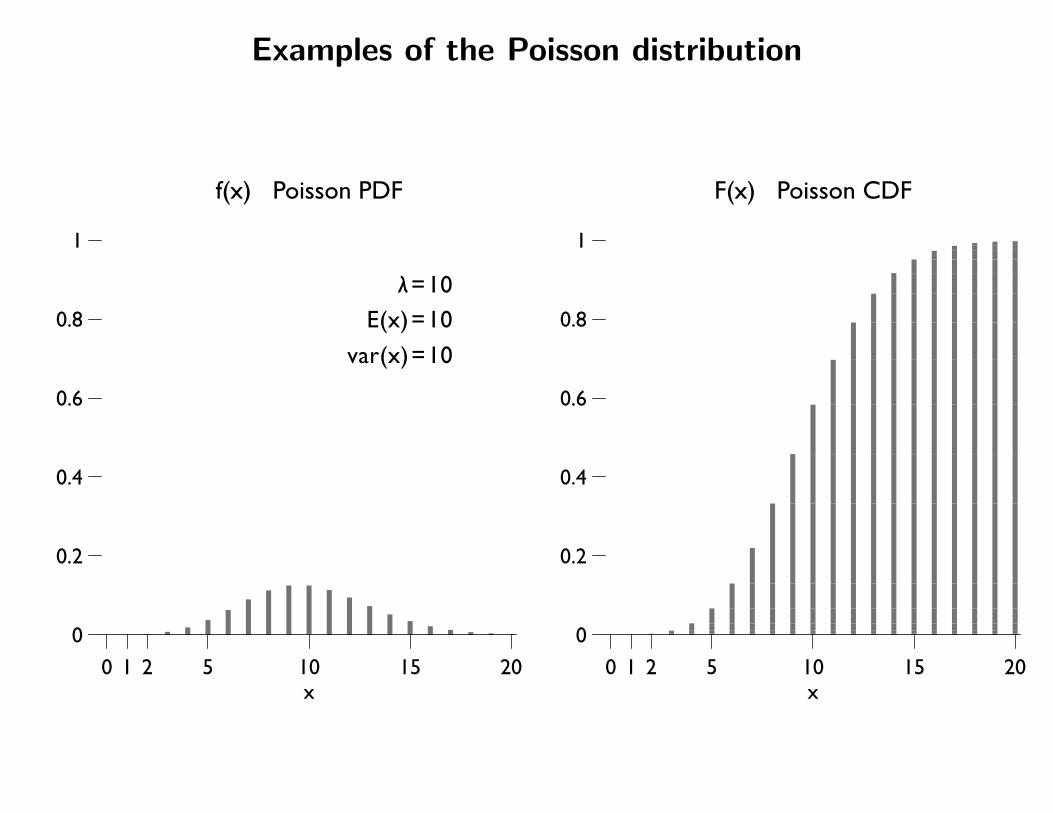
λ=10E(x)=10
var(x)=10
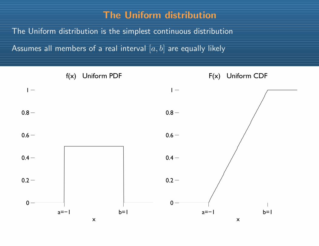
The Uniform distribution
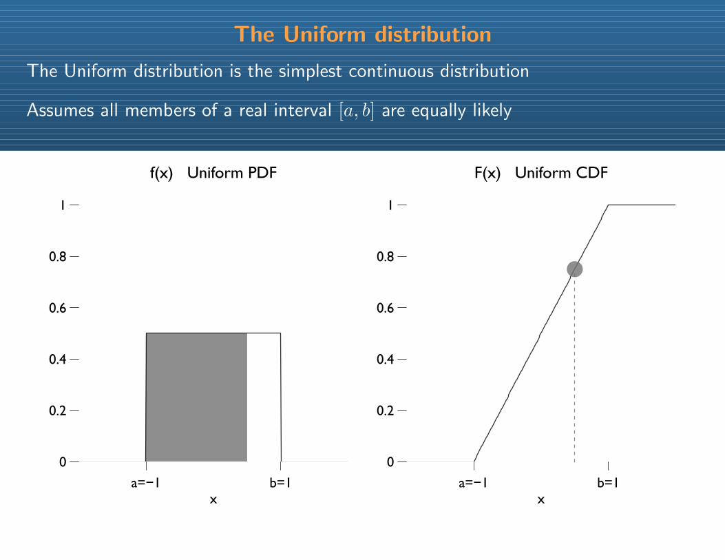
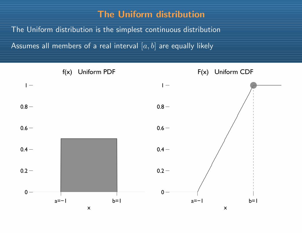
The Uniform distribution is the simplest continuous distribution
Assumes all members of a real interval [a, b] are equally likely
a=−1 b=1
0
0.2
0.4
0.6
0.8
1
f(x) Uniform PDF
xa=−1 b=1
0
0.2
0.4
0.6
0.8
1
F(x) Uniform CDF
x
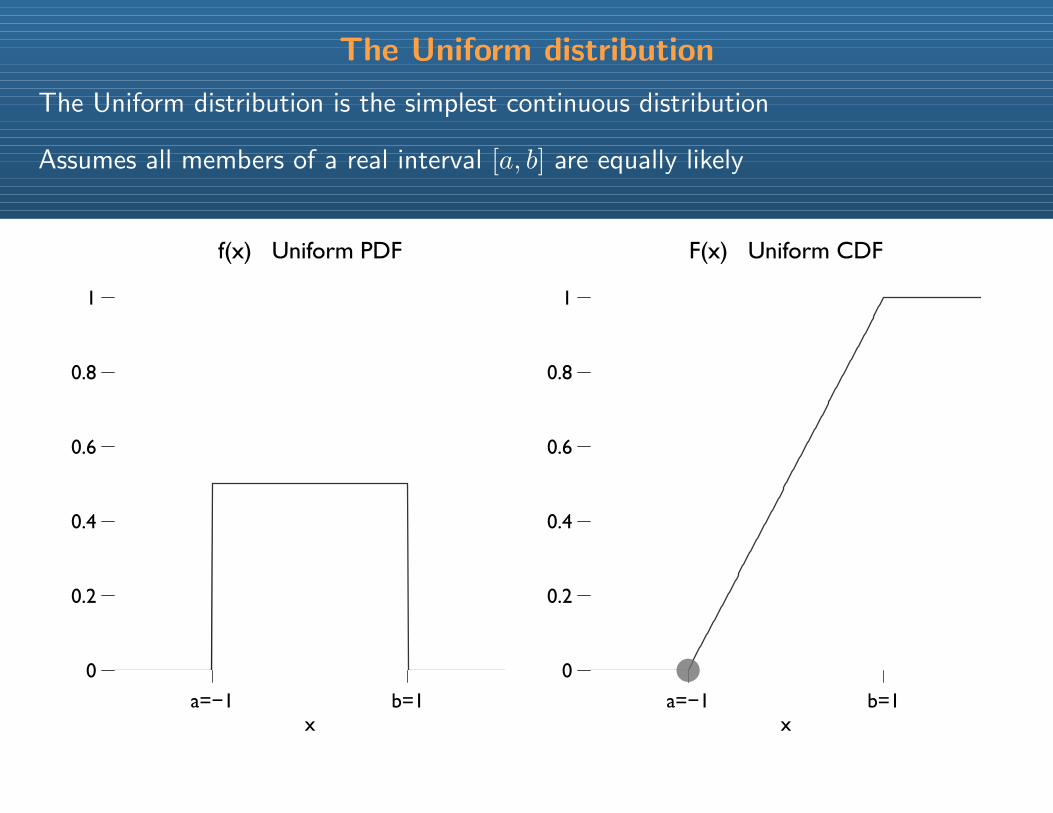
The Uniform distribution
The Uniform distribution is the simplest continuous distribution
Assumes all members of a real interval [a, b] are equally likely
a=−1 b=1
0
0.2
0.4
0.6
0.8
1
f(x) Uniform PDF
xa=−1 b=1
0
0.2
0.4
0.6
0.8
1
F(x) Uniform CDF
x
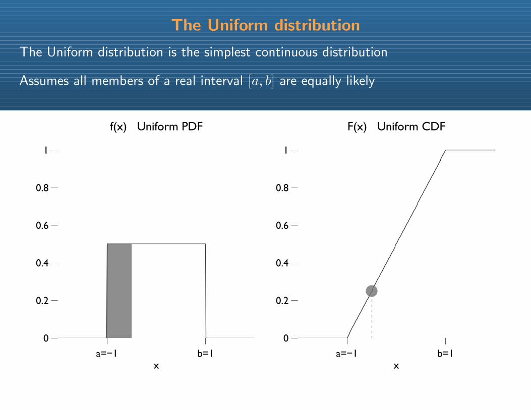
The Uniform distribution
The Uniform distribution is the simplest continuous distribution
Assumes all members of a real interval [a, b] are equally likely
a=−1 b=1
0
0.2
0.4
0.6
0.8
1
f(x) Uniform PDF
xa=−1 b=1
0
0.2
0.4
0.6
0.8
1
F(x) Uniform CDF
x
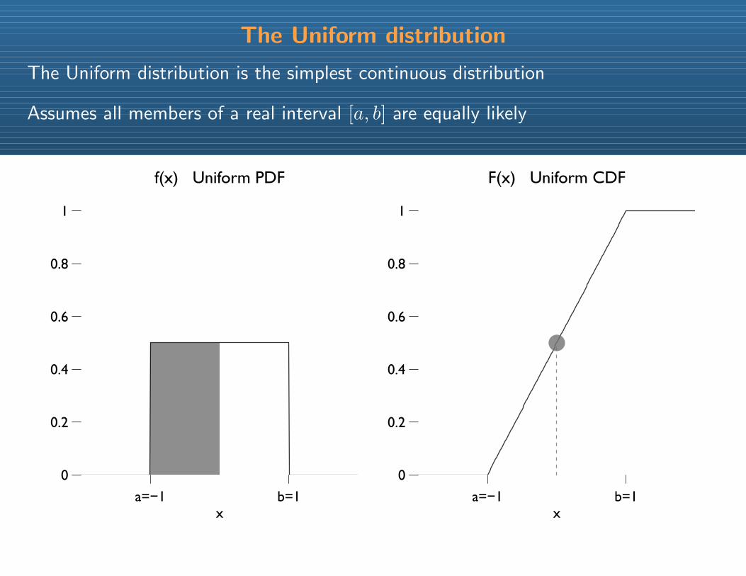
The Uniform distribution
The Uniform distribution is the simplest continuous distribution
Assumes all members of a real interval [a, b] are equally likely
a=−1 b=1
0
0.2
0.4
0.6
0.8
1
f(x) Uniform PDF
xa=−1 b=1
0
0.2
0.4
0.6
0.8
1
F(x) Uniform CDF
x
The Uniform distribution
The Uniform distribution is the simplest continuous distribution
Assumes all members of a real interval [a, b] are equally likely
a=−1 b=1
0
0.2
0.4
0.6
0.8
1
f(x) Uniform PDF
xa=−1 b=1
0
0.2
0.4
0.6
0.8
1
F(x) Uniform CDF
x
The Uniform distribution
The Uniform distribution is the simplest continuous distribution
Assumes all members of a real interval [a, b] are equally likely
a=−1 b=1
0
0.2
0.4
0.6
0.8
1
f(x) Uniform PDF
xa=−1 b=1
0
0.2
0.4
0.6
0.8
1
F(x) Uniform CDF
x
The uniform distribution
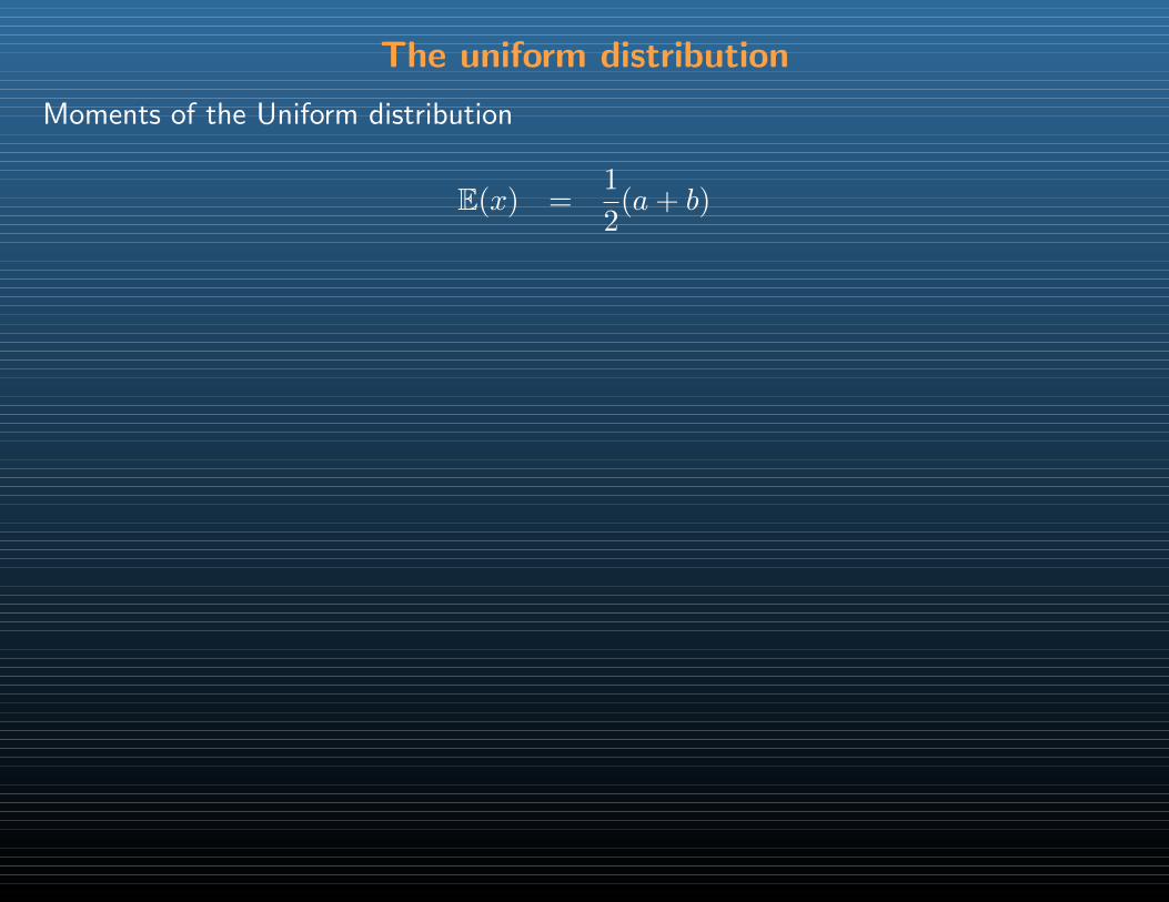
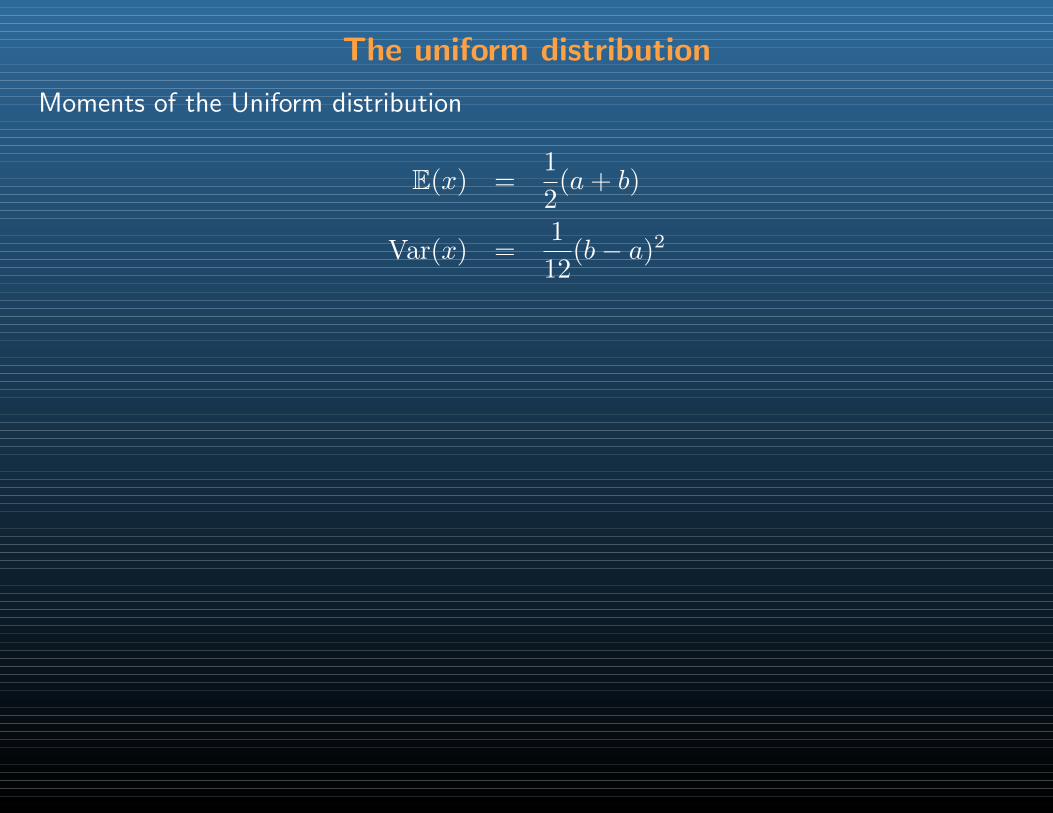
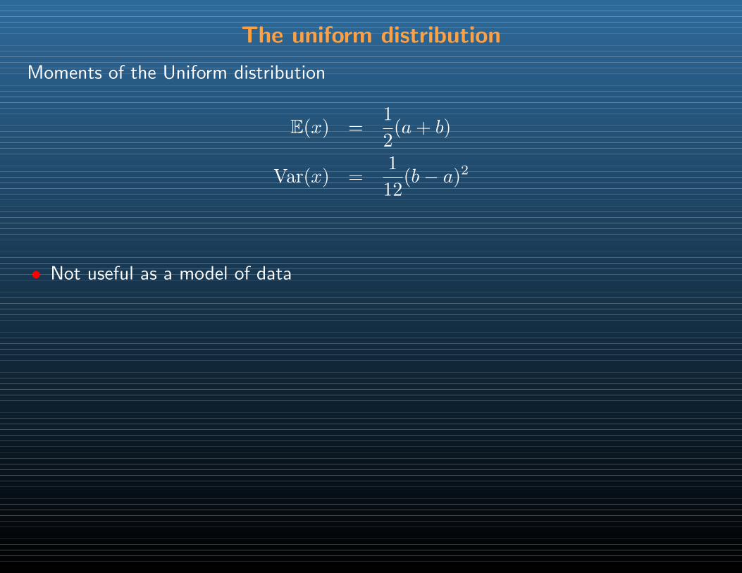
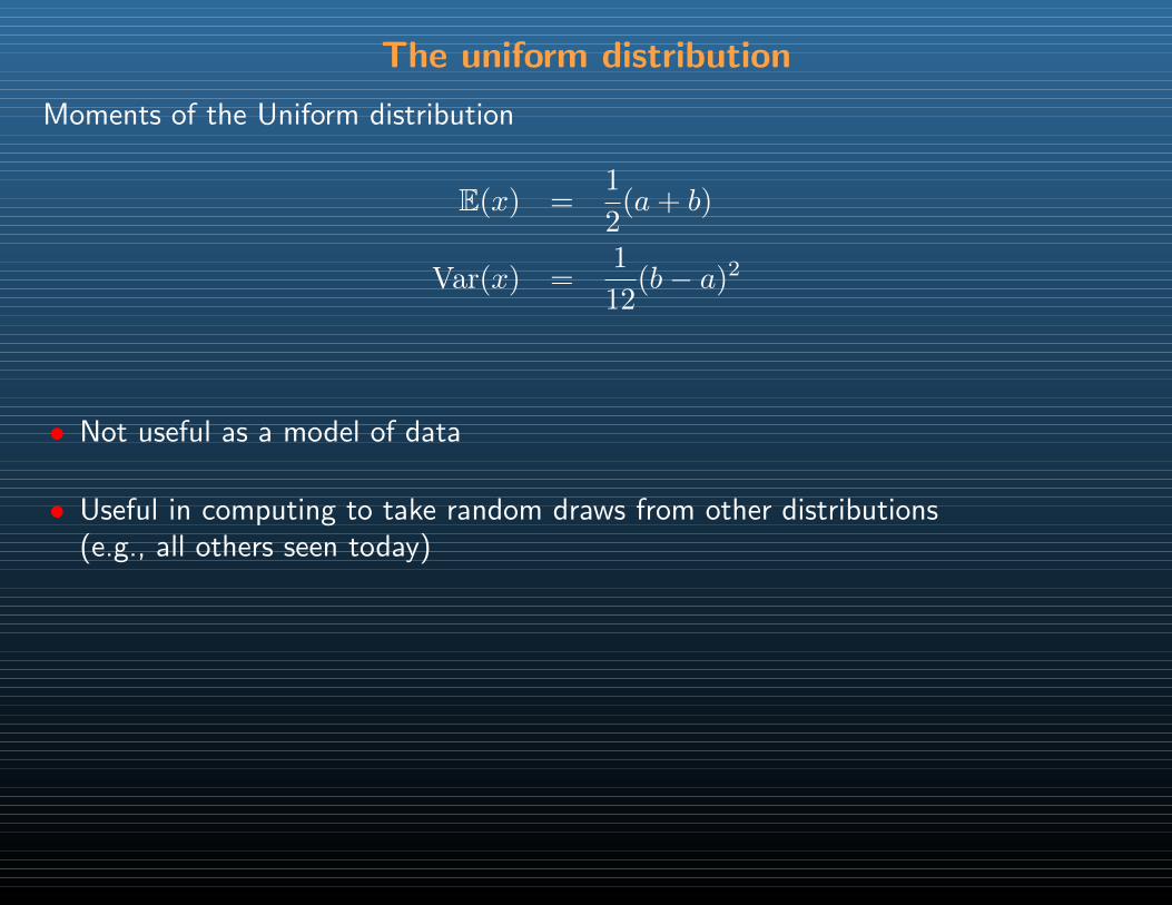
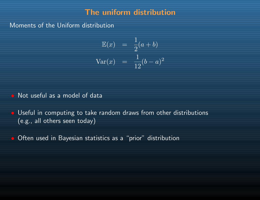
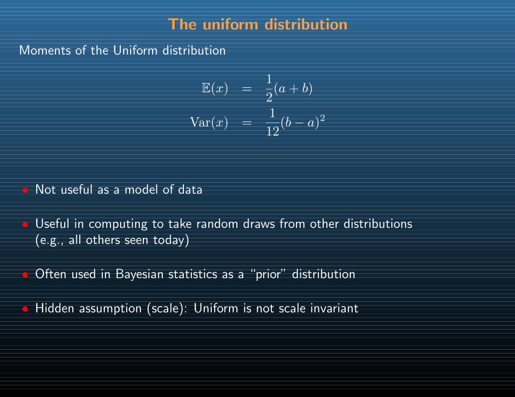
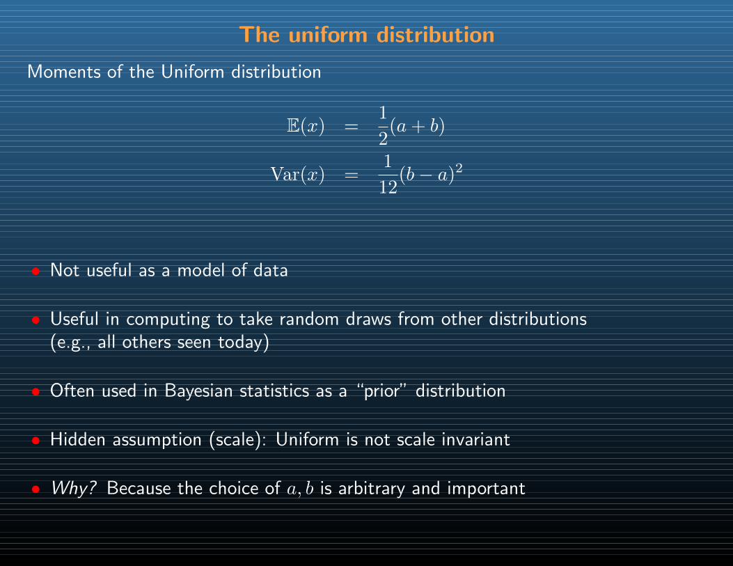
Moments of the Uniform distribution
E(x) =1
2(a+ b)
The uniform distribution
Moments of the Uniform distribution
E(x) =1
2(a+ b)
Var(x) =1
12(b− a)2
The uniform distribution
Moments of the Uniform distribution
E(x) =1
2(a+ b)
Var(x) =1
12(b− a)2
• Not useful as a model of data
The uniform distribution
Moments of the Uniform distribution
E(x) =1
2(a+ b)
Var(x) =1
12(b− a)2
• Not useful as a model of data
• Useful in computing to take random draws from other distributions(e.g., all others seen today)
The uniform distribution
Moments of the Uniform distribution
E(x) =1
2(a+ b)
Var(x) =1
12(b− a)2
• Not useful as a model of data
• Useful in computing to take random draws from other distributions(e.g., all others seen today)
• Often used in Bayesian statistics as a “prior” distribution
The uniform distribution
Moments of the Uniform distribution
E(x) =1
2(a+ b)
Var(x) =1
12(b− a)2
• Not useful as a model of data
• Useful in computing to take random draws from other distributions(e.g., all others seen today)
• Often used in Bayesian statistics as a “prior” distribution
• Hidden assumption (scale): Uniform is not scale invariant
• Why? Because the choice of a, b is arbitrary and important
The Normal (or Gaussian) distribution
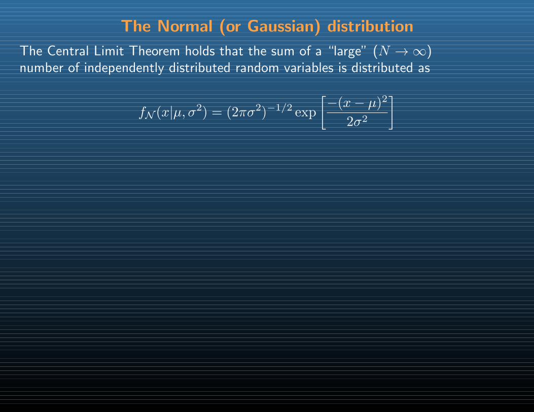
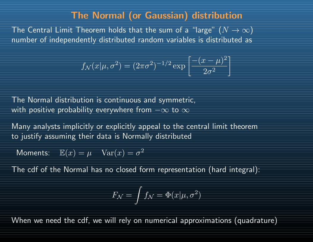
The Central Limit Theorem holds that the sum of a “large” (N →∞)number of independently distributed random variables is distributed as
fN (x|µ, σ2) = (2πσ2)−1/2 exp
[−(x− µ)2
2σ2
]
The Normal (or Gaussian) distribution
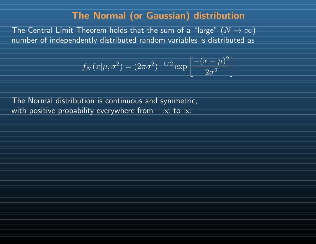
The Central Limit Theorem holds that the sum of a “large” (N →∞)number of independently distributed random variables is distributed as
fN (x|µ, σ2) = (2πσ2)−1/2 exp
[−(x− µ)2
2σ2
]
The Normal distribution is continuous and symmetric,with positive probability everywhere from −∞ to ∞

The Normal (or Gaussian) distribution
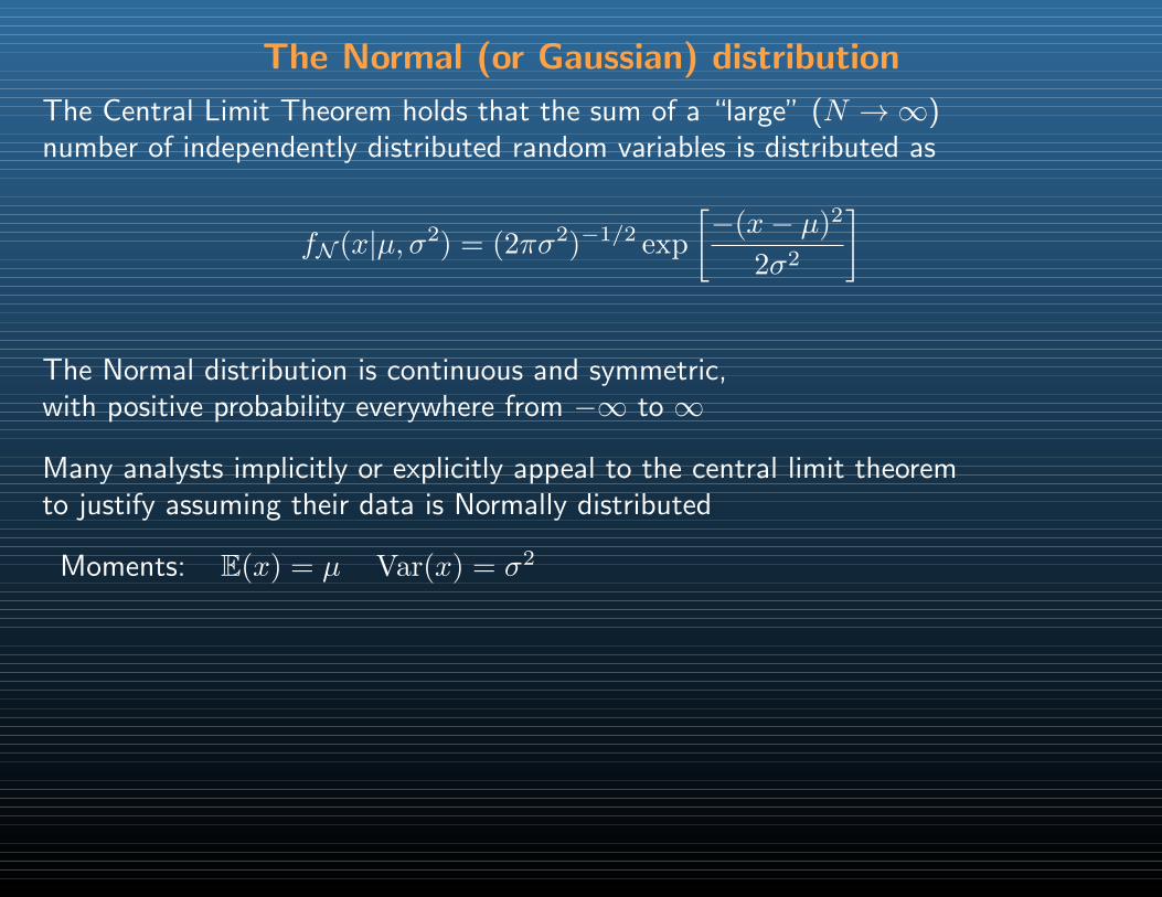
The Central Limit Theorem holds that the sum of a “large” (N →∞)number of independently distributed random variables is distributed as
fN (x|µ, σ2) = (2πσ2)−1/2 exp
[−(x− µ)2
2σ2
]
The Normal distribution is continuous and symmetric,with positive probability everywhere from −∞ to ∞
Many analysts implicitly or explicitly appeal to the central limit theoremto justify assuming their data is Normally distributed
The Normal (or Gaussian) distribution
The Central Limit Theorem holds that the sum of a “large” (N →∞)number of independently distributed random variables is distributed as
fN (x|µ, σ2) = (2πσ2)−1/2 exp
[−(x− µ)2
2σ2
]
The Normal distribution is continuous and symmetric,with positive probability everywhere from −∞ to ∞
Many analysts implicitly or explicitly appeal to the central limit theoremto justify assuming their data is Normally distributed
Moments: E(x) = µ Var(x) = σ2
The cdf of the Normal has no closed form representation (hard integral):
FN =
∫fN = Φ(x|µ, σ2)
When we need the cdf, we will rely on numerical approximations (quadrature)
The Normal (Gaussian) distribution
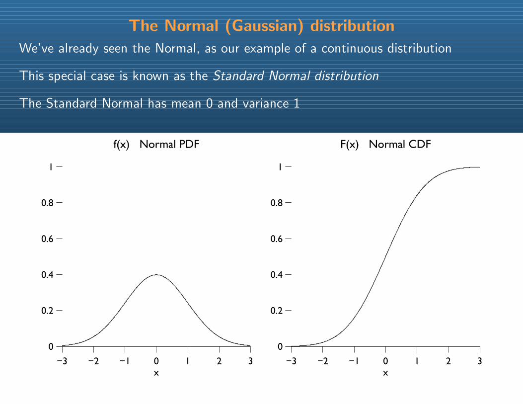
We’ve already seen the Normal, as our example of a continuous distribution
This special case is known as the Standard Normal distribution
The Standard Normal has mean 0 and variance 1
−3 −2 −1 0 1 2 3
0
0.2
0.4
0.6
0.8
1
f(x) Normal PDF
x−3 −2 −1 0 1 2 3
0
0.2
0.4
0.6
0.8
1
F(x) Normal CDF
x
The Normal (Gaussian) distribution
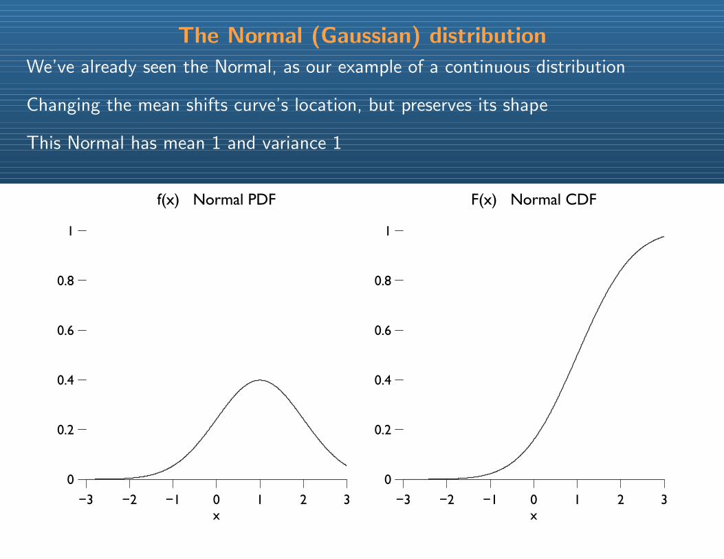
We’ve already seen the Normal, as our example of a continuous distribution
Changing the mean shifts curve’s location, but preserves its shape
This Normal has mean 1 and variance 1
−3 −2 −1 0 1 2 3
0
0.2
0.4
0.6
0.8
1
f(x) Normal PDF
x−3 −2 −1 0 1 2 3
0
0.2
0.4
0.6
0.8
1
F(x) Normal CDF
x
The Normal (Gaussian) distribution
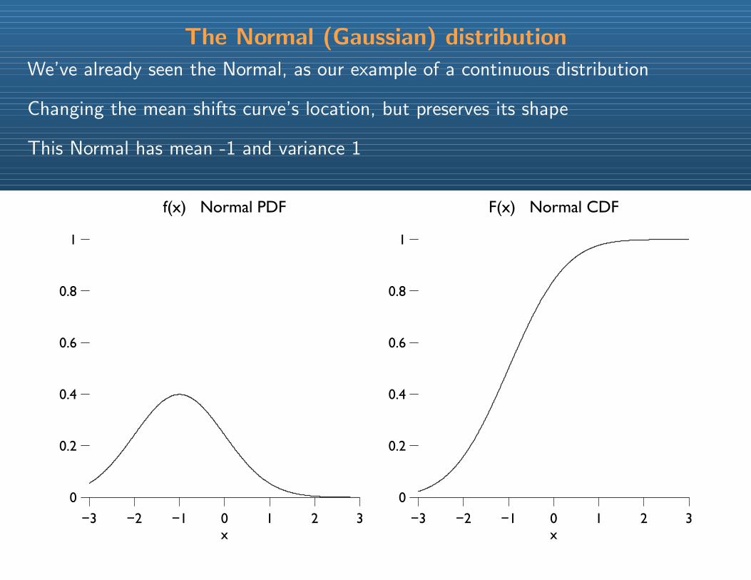
We’ve already seen the Normal, as our example of a continuous distribution
Changing the mean shifts curve’s location, but preserves its shape
This Normal has mean -1 and variance 1
−3 −2 −1 0 1 2 3
0
0.2
0.4
0.6
0.8
1
f(x) Normal PDF
x−3 −2 −1 0 1 2 3
0
0.2
0.4
0.6
0.8
1
F(x) Normal CDF
x
The Normal (Gaussian) distribution
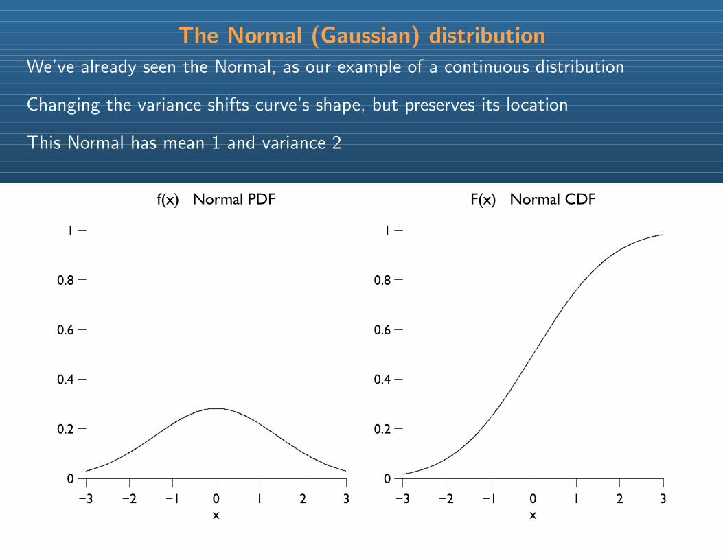
We’ve already seen the Normal, as our example of a continuous distribution
Changing the variance shifts curve’s shape, but preserves its location
This Normal has mean 1 and variance 2
−3 −2 −1 0 1 2 3
0
0.2
0.4
0.6
0.8
1
f(x) Normal PDF
x−3 −2 −1 0 1 2 3
0
0.2
0.4
0.6
0.8
1
F(x) Normal CDF
x
The Normal (Gaussian) distribution
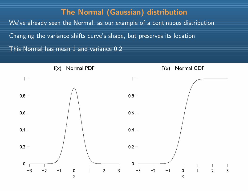
We’ve already seen the Normal, as our example of a continuous distribution
Changing the variance shifts curve’s shape, but preserves its location
This Normal has mean 1 and variance 0.2
−3 −2 −1 0 1 2 3
0
0.2
0.4
0.6
0.8
1
f(x) Normal PDF
x−3 −2 −1 0 1 2 3
0
0.2
0.4
0.6
0.8
1
F(x) Normal CDF
x
Why R?
Real question: Why programming?
Non-programmers are stuck with package defaults
For your substantive problem, these default settings may be
• inappropriate (not quite the right model, but “close”)
• unintelligible (reams of non-linear coefficients and stars)
Programming allows you to match the methods to the data & question
Get better, more easily explained results.
Why R?
Many side benefits:
1. Never forget what you did: The code can be re-run.
2. Repeating an analysis n times? Write a loop!
3. Programming makes data processing/reshaping easy.
4. Programming makes replication easy.

Why R?
R is
• free
• open source
• growing fast
• widely used
• the future for most fields
But once you learn one language, the others are much easier
Introduction to R
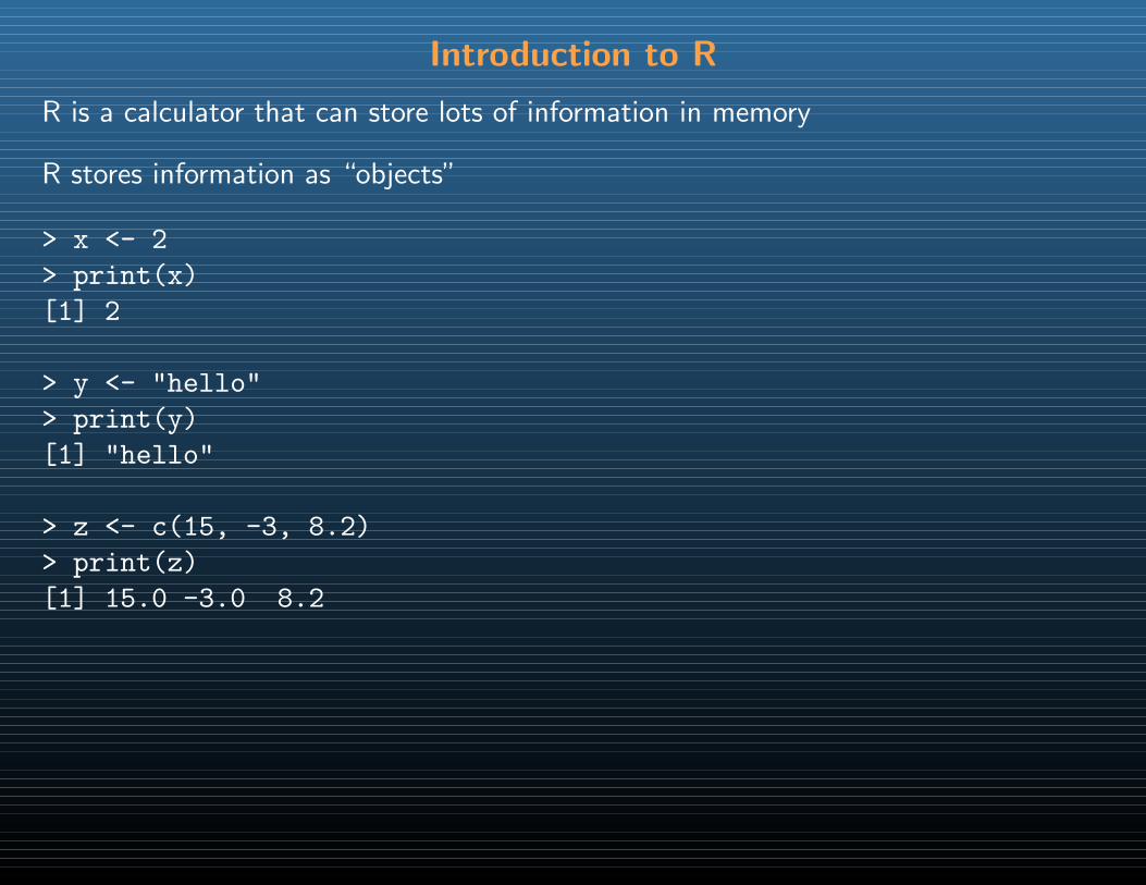
R is a calculator that can store lots of information in memory
R stores information as “objects”
> x <- 2
> print(x)
[1] 2
> y <- "hello"
> print(y)
[1] "hello"
> z <- c(15, -3, 8.2)
> print(z)
[1] 15.0 -3.0 8.2

Introduction to R
> w <- c("gdp", "pop", "income")
> print(w)
[1] "gdp" "pop" "income"
>
Note the assignment operator, <-, not =
An object in memory can be called to make new objects
> a <- x^2
> print(x)
[1] 2
> print(a)
[1] 4
> b <- z + 10
> print(z)
[1] 15.0 -3.0 8.2
> print(b)
[1] 25.0 7.0 18.2
Introduction to R
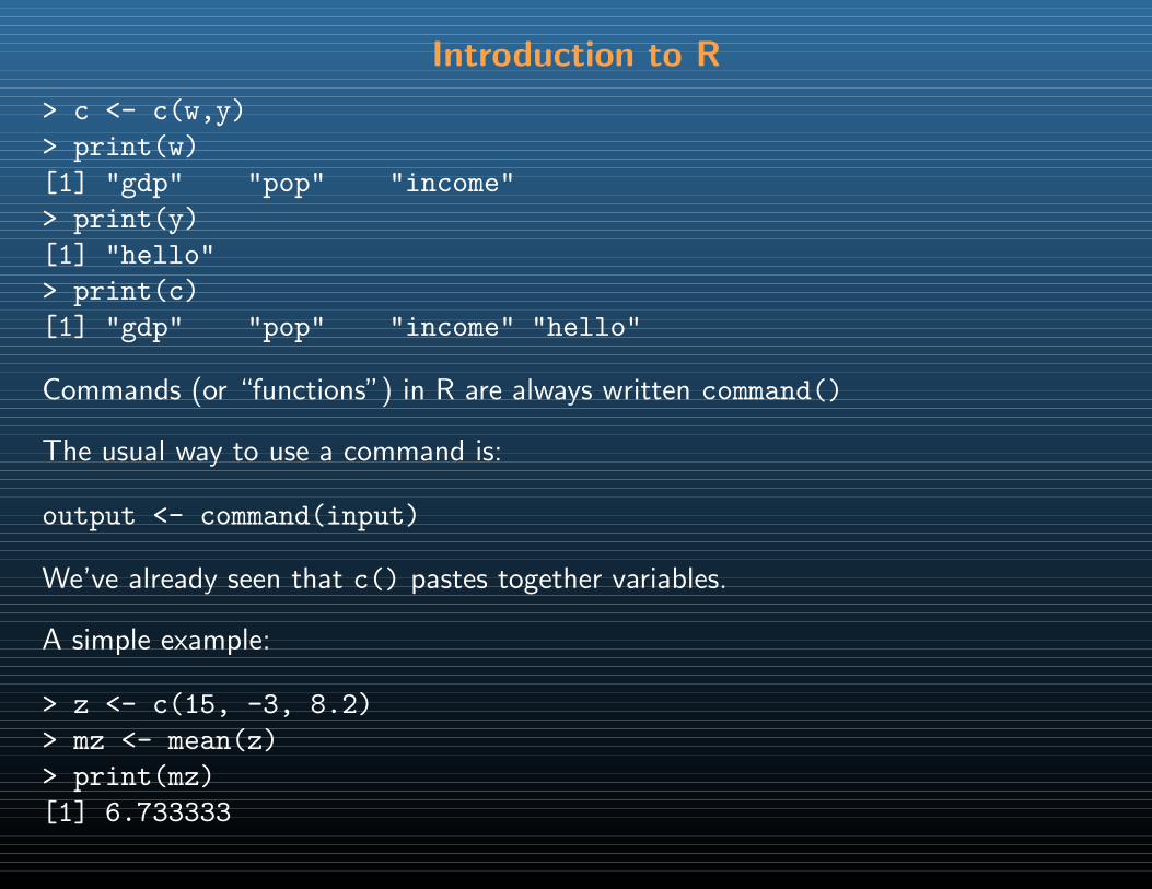
> c <- c(w,y)
> print(w)
[1] "gdp" "pop" "income"
> print(y)
[1] "hello"
> print(c)
[1] "gdp" "pop" "income" "hello"
Commands (or “functions”) in R are always written command()
The usual way to use a command is:
output <- command(input)
We’ve already seen that c() pastes together variables.
A simple example:
> z <- c(15, -3, 8.2)
> mz <- mean(z)
> print(mz)
[1] 6.733333
Introduction to R
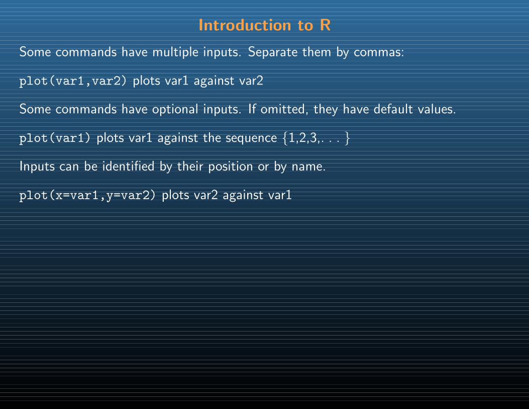
Some commands have multiple inputs. Separate them by commas:
plot(var1,var2) plots var1 against var2
Some commands have optional inputs. If omitted, they have default values.
plot(var1) plots var1 against the sequence 1,2,3,. . .
Inputs can be identified by their position or by name.
plot(x=var1,y=var2) plots var2 against var1
Entering code
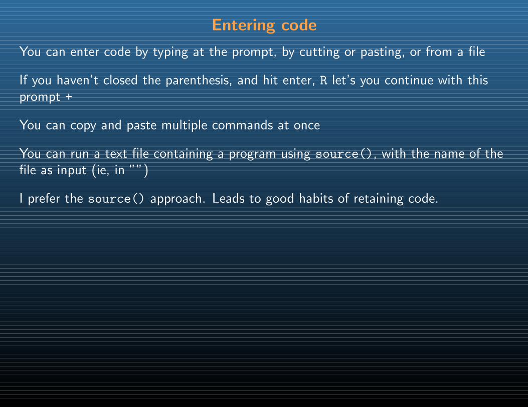
You can enter code by typing at the prompt, by cutting or pasting, or from a file
If you haven’t closed the parenthesis, and hit enter, R let’s you continue with thisprompt +
You can copy and paste multiple commands at once
You can run a text file containing a program using source(), with the name of thefile as input (ie, in ””)
I prefer the source() approach. Leads to good habits of retaining code.
Data types
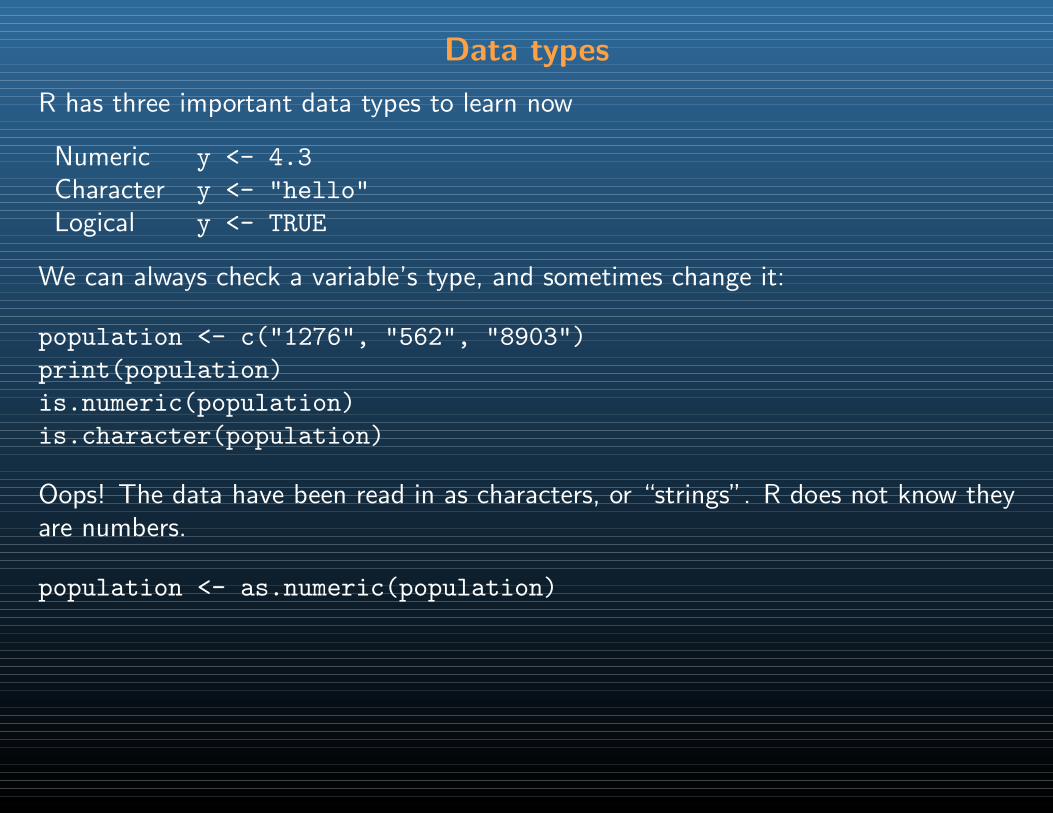
R has three important data types to learn now
Numeric y <- 4.3
Character y <- "hello"
Logical y <- TRUE
We can always check a variable’s type, and sometimes change it:
population <- c("1276", "562", "8903")
print(population)
is.numeric(population)
is.character(population)
Oops! The data have been read in as characters, or “strings”. R does not know theyare numbers.
population <- as.numeric(population)
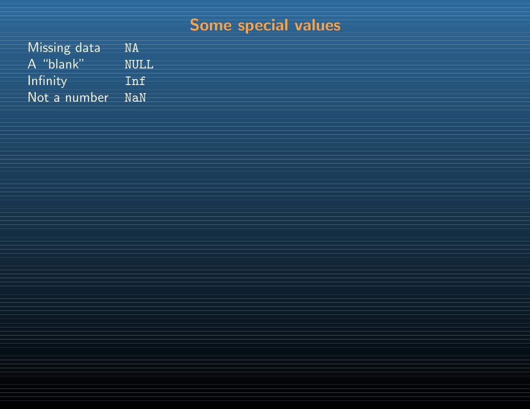
Some special values
Missing data NA
A “blank” NULL
Infinity Inf
Not a number NaN
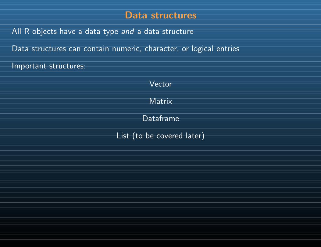
Data structures
All R objects have a data type and a data structure
Data structures can contain numeric, character, or logical entries
Important structures:
Vector
Matrix
Dataframe
List (to be covered later)
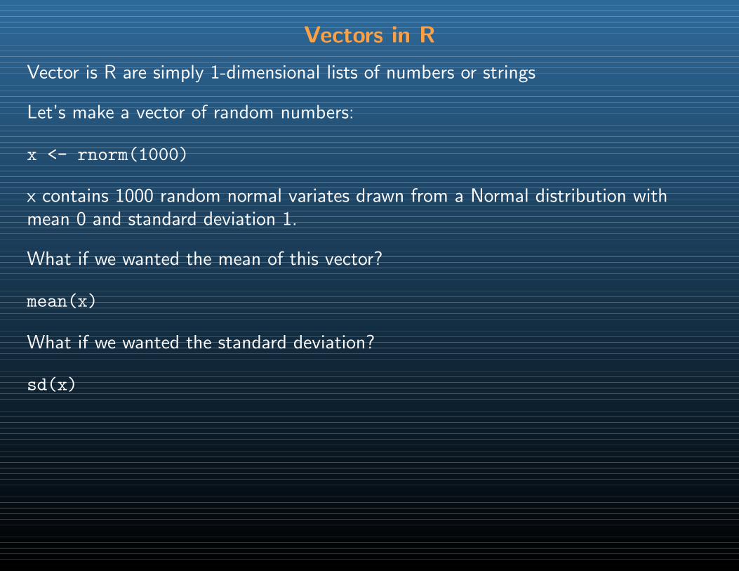
Vectors in R
Vector is R are simply 1-dimensional lists of numbers or strings
Let’s make a vector of random numbers:
x <- rnorm(1000)
x contains 1000 random normal variates drawn from a Normal distribution withmean 0 and standard deviation 1.
What if we wanted the mean of this vector?
mean(x)
What if we wanted the standard deviation?
sd(x)
Vectors in R
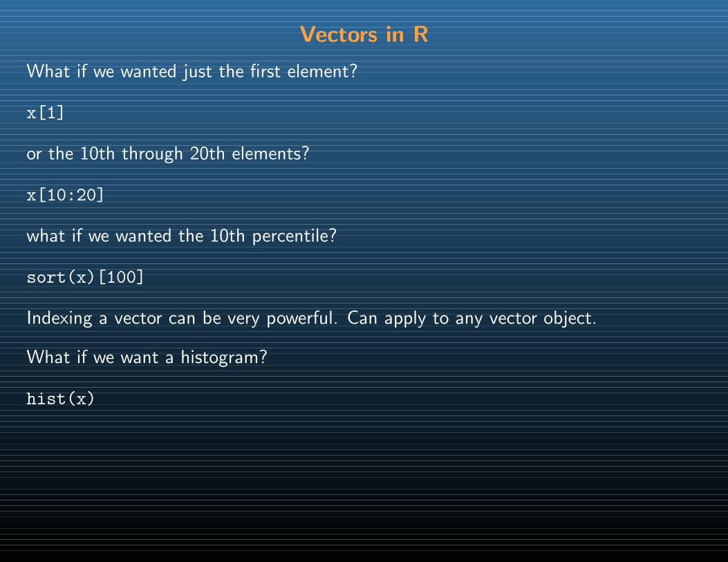
What if we wanted just the first element?
x[1]
or the 10th through 20th elements?
x[10:20]
what if we wanted the 10th percentile?
sort(x)[100]
Indexing a vector can be very powerful. Can apply to any vector object.
What if we want a histogram?
hist(x)
Vectors in R
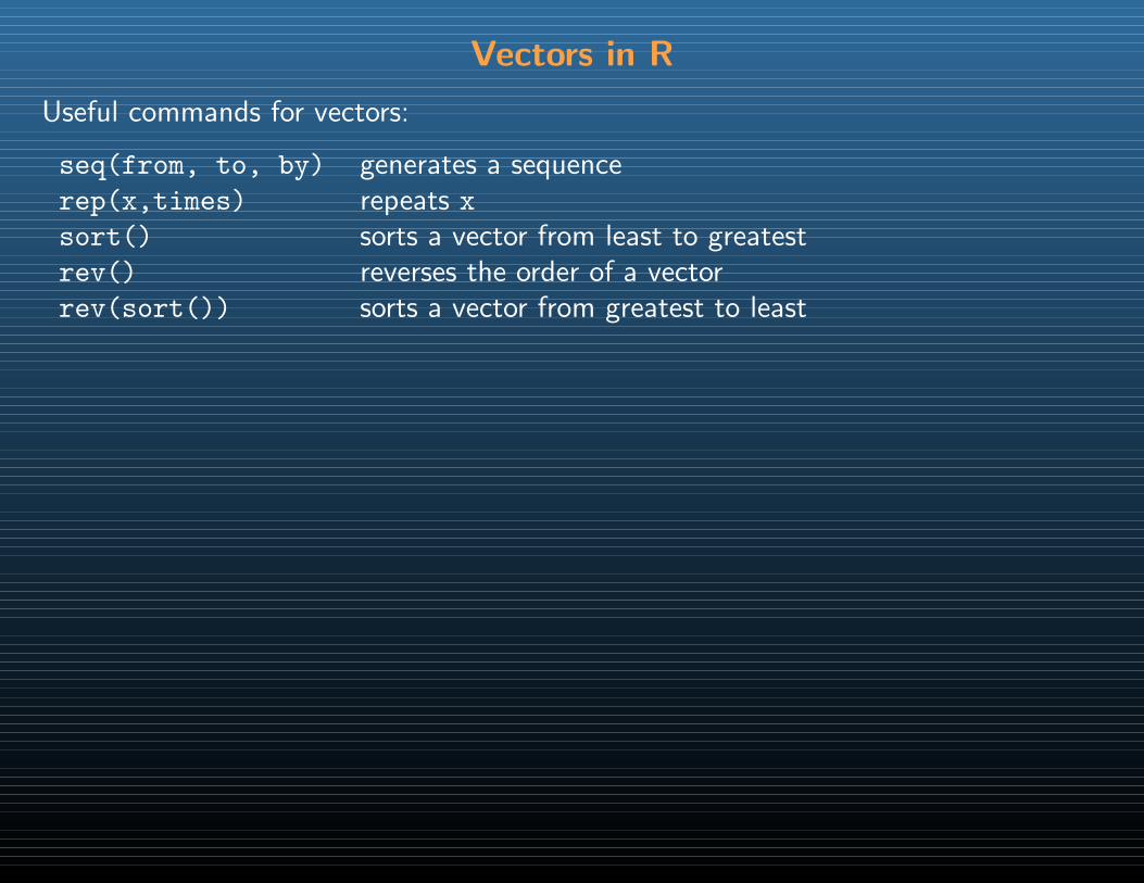
Useful commands for vectors:
seq(from, to, by) generates a sequencerep(x,times) repeats x
sort() sorts a vector from least to greatestrev() reverses the order of a vectorrev(sort()) sorts a vector from greatest to least

Matrices in R
Vector are the standard way to store and manipulate variables in R
But usually our datasets have several variables measured on the same observations
Several variables collected together form a matrix with one row for each observationand one column for each variable
Matrices in R
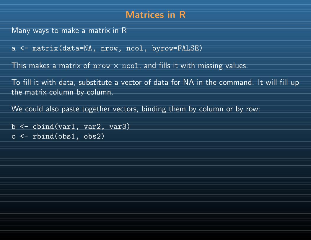
Many ways to make a matrix in R
a <- matrix(data=NA, nrow, ncol, byrow=FALSE)
This makes a matrix of nrow × ncol, and fills it with missing values.
To fill it with data, substitute a vector of data for NA in the command. It will fill upthe matrix column by column.
We could also paste together vectors, binding them by column or by row:
b <- cbind(var1, var2, var3)
c <- rbind(obs1, obs2)
Matrices in R
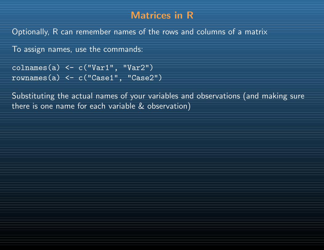
Optionally, R can remember names of the rows and columns of a matrix
To assign names, use the commands:
colnames(a) <- c("Var1", "Var2")
rownames(a) <- c("Case1", "Case2")
Substituting the actual names of your variables and observations (and making surethere is one name for each variable & observation)
Matrices in R
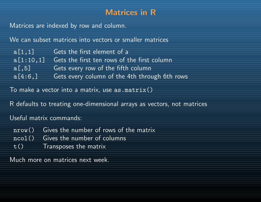
Matrices are indexed by row and column.
We can subset matrices into vectors or smaller matrices
a[1,1] Gets the first element of aa[1:10,1] Gets the first ten rows of the first columna[,5] Gets every row of the fifth columna[4:6,] Gets every column of the 4th through 6th rows
To make a vector into a matrix, use as.matrix()
R defaults to treating one-dimensional arrays as vectors, not matrices
Useful matrix commands:
nrow() Gives the number of rows of the matrixncol() Gives the number of columnst() Transposes the matrix
Much more on matrices next week.
Dataframes in R
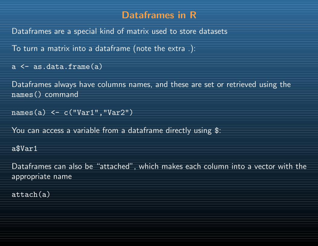
Dataframes are a special kind of matrix used to store datasets
To turn a matrix into a dataframe (note the extra .):
a <- as.data.frame(a)
Dataframes always have columns names, and these are set or retrieved using thenames() command
names(a) <- c("Var1","Var2")
You can access a variable from a dataframe directly using $:
a$Var1
Dataframes can also be “attached”, which makes each column into a vector with theappropriate name
attach(a)
Loading data
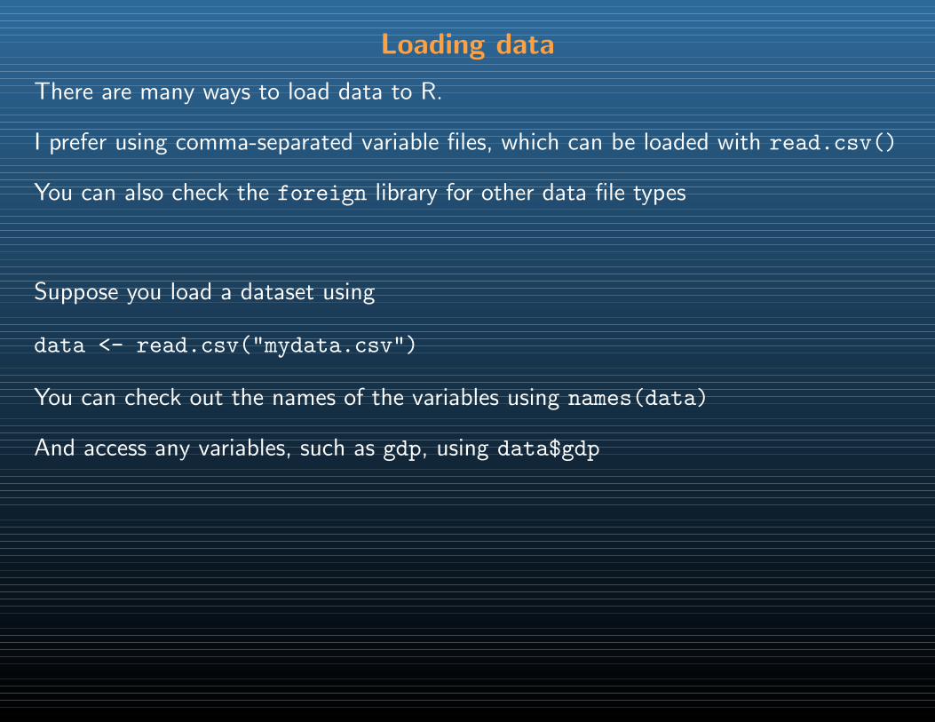
There are many ways to load data to R.
I prefer using comma-separated variable files, which can be loaded with read.csv()
You can also check the foreign library for other data file types
Suppose you load a dataset using
data <- read.csv("mydata.csv")
You can check out the names of the variables using names(data)
And access any variables, such as gdp, using data$gdp
Benefits and dangers of attach()
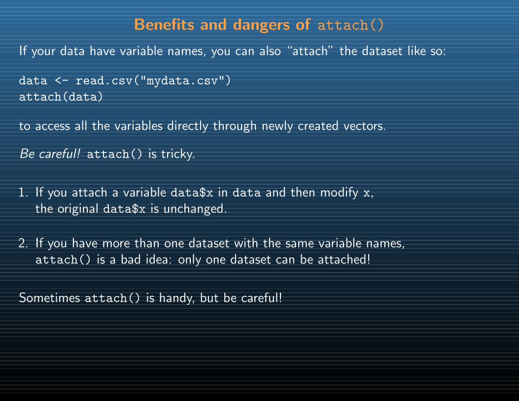
If your data have variable names, you can also “attach” the dataset like so:
data <- read.csv("mydata.csv")
attach(data)
to access all the variables directly through newly created vectors.
Be careful! attach() is tricky.
1. If you attach a variable data$x in data and then modify x,the original data$x is unchanged.
2. If you have more than one dataset with the same variable names,attach() is a bad idea: only one dataset can be attached!
Sometimes attach() is handy, but be careful!
Missing data
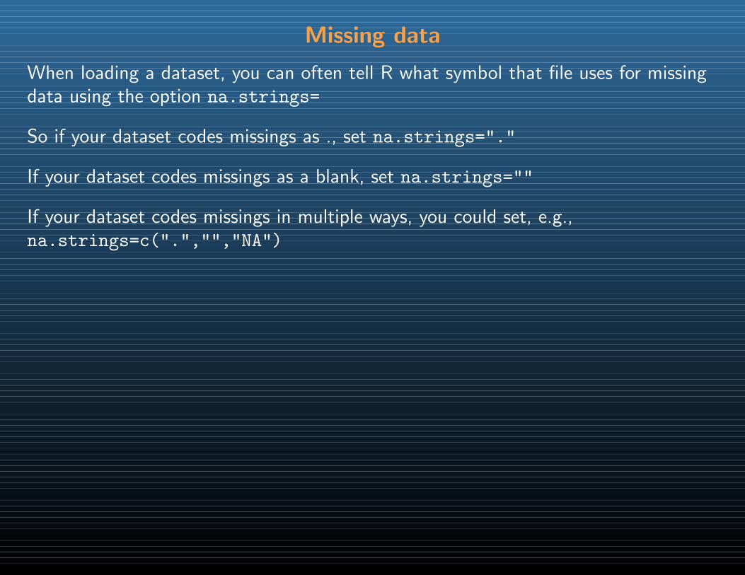
When loading a dataset, you can often tell R what symbol that file uses for missingdata using the option na.strings=
So if your dataset codes missings as ., set na.strings="."
If your dataset codes missings as a blank, set na.strings=""
If your dataset codes missings in multiple ways, you could set, e.g.,na.strings=c(".","","NA")
Missing data
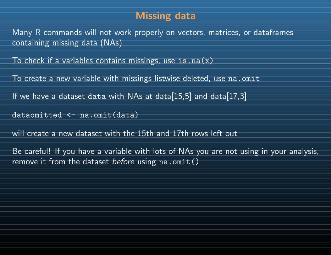
Many R commands will not work properly on vectors, matrices, or dataframescontaining missing data (NAs)
To check if a variables contains missings, use is.na(x)
To create a new variable with missings listwise deleted, use na.omit
If we have a dataset data with NAs at data[15,5] and data[17,3]
dataomitted <- na.omit(data)
will create a new dataset with the 15th and 17th rows left out
Be careful! If you have a variable with lots of NAs you are not using in your analysis,remove it from the dataset before using na.omit()
Mathematical Operations
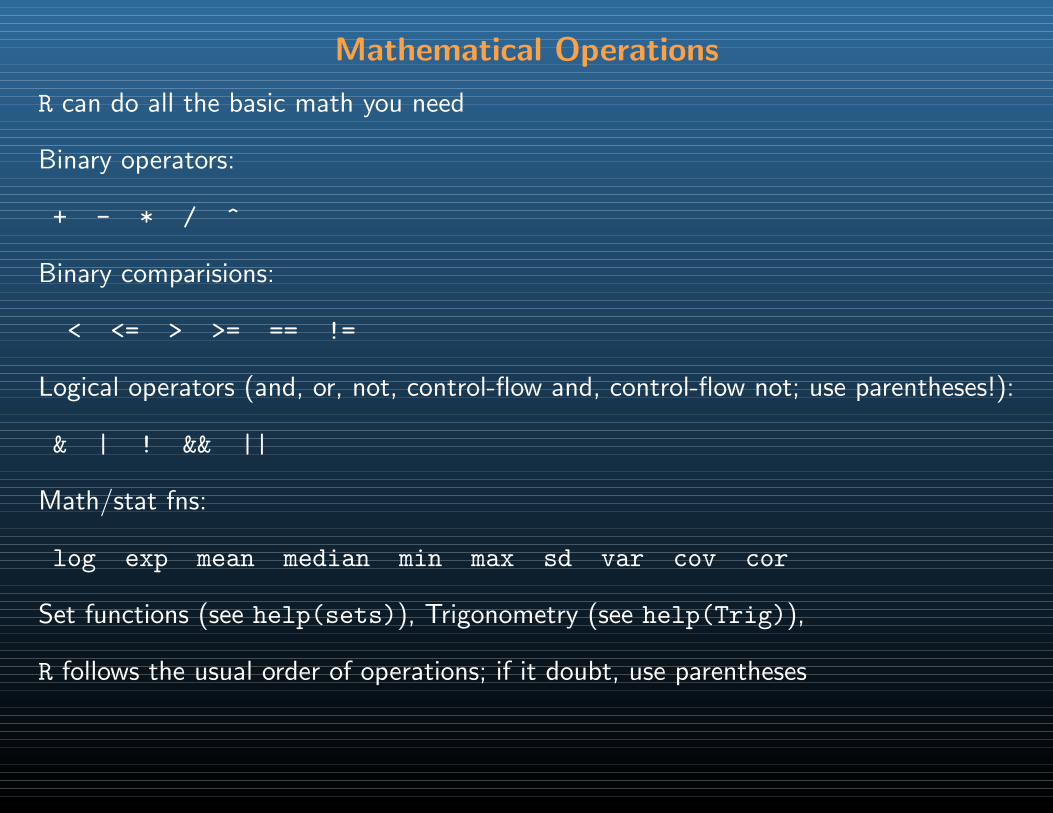
R can do all the basic math you need
Binary operators:
+ - * / ^
Binary comparisions:
< <= > >= == !=
Logical operators (and, or, not, control-flow and, control-flow not; use parentheses!):
& | ! && ||
Math/stat fns:
log exp mean median min max sd var cov cor
Set functions (see help(sets)), Trigonometry (see help(Trig)),
R follows the usual order of operations; if it doubt, use parentheses
Example 1: US Economic growth
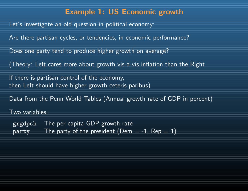
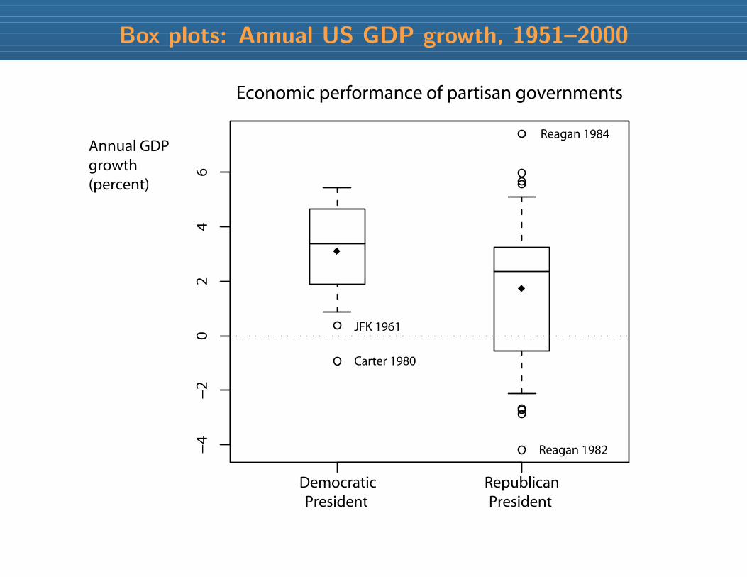
Let’s investigate an old question in political economy:
Are there partisan cycles, or tendencies, in economic performance?
Does one party tend to produce higher growth on average?
(Theory: Left cares more about growth vis-a-vis inflation than the Right
If there is partisan control of the economy,then Left should have higher growth ceteris paribus)
Data from the Penn World Tables (Annual growth rate of GDP in percent)
Two variables:
grgdpch The per capita GDP growth rateparty The party of the president (Dem = -1, Rep = 1)
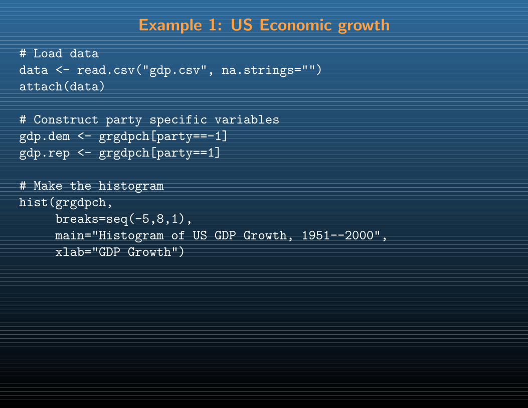
Example 1: US Economic growth
# Load data
data <- read.csv("gdp.csv", na.strings="")
attach(data)
# Construct party specific variables
gdp.dem <- grgdpch[party==-1]
gdp.rep <- grgdpch[party==1]
# Make the histogram
hist(grgdpch,
breaks=seq(-5,8,1),
main="Histogram of US GDP Growth, 1951--2000",
xlab="GDP Growth")
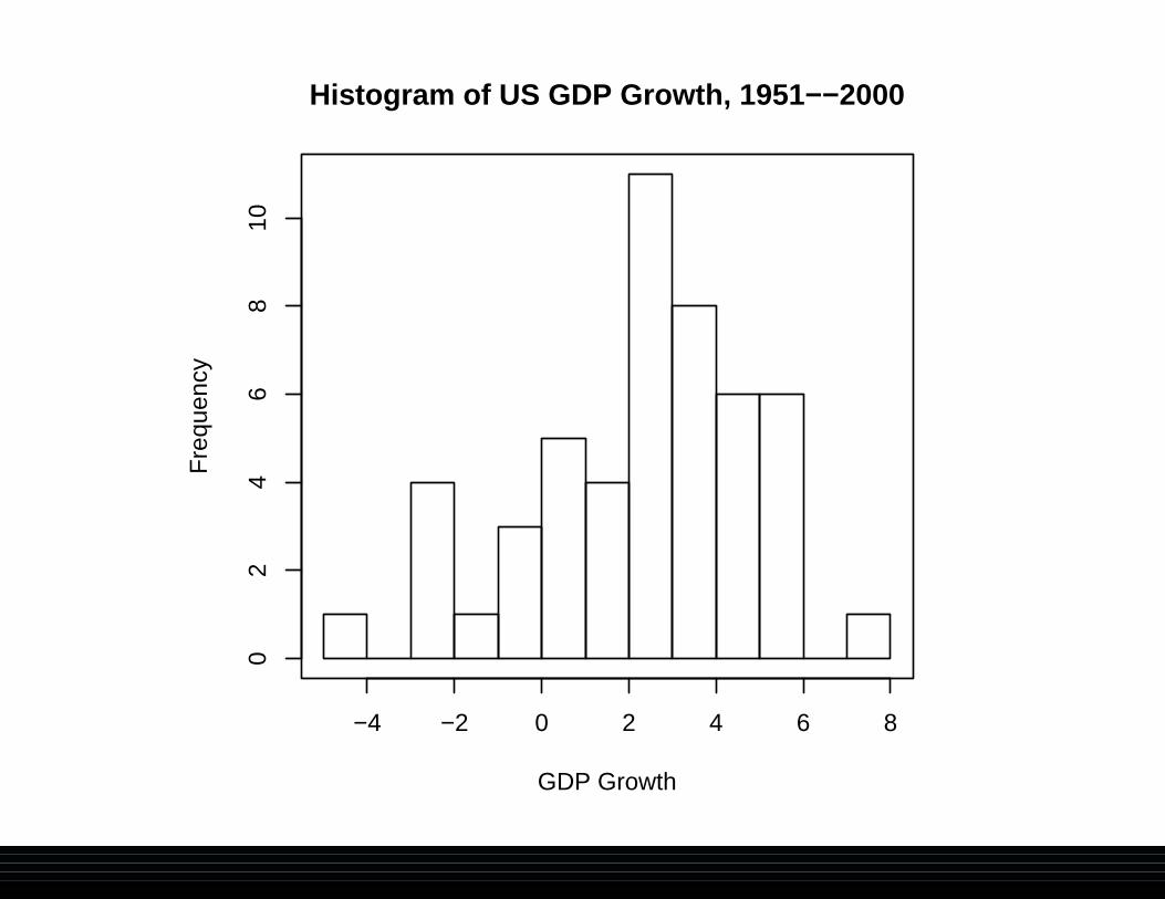
Histogram of US GDP Growth, 1951−−2000
GDP Growth
Fre
quen
cy
−4 −2 0 2 4 6 8
02
46
810
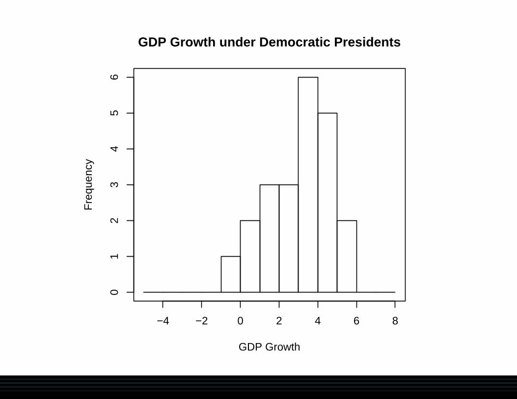
GDP Growth under Democratic Presidents
GDP Growth
Fre
quen
cy
−4 −2 0 2 4 6 8
01
23
45
6
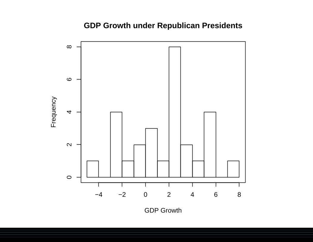
GDP Growth under Republican Presidents
GDP Growth
Fre
quen
cy
−4 −2 0 2 4 6 8
02
46
8
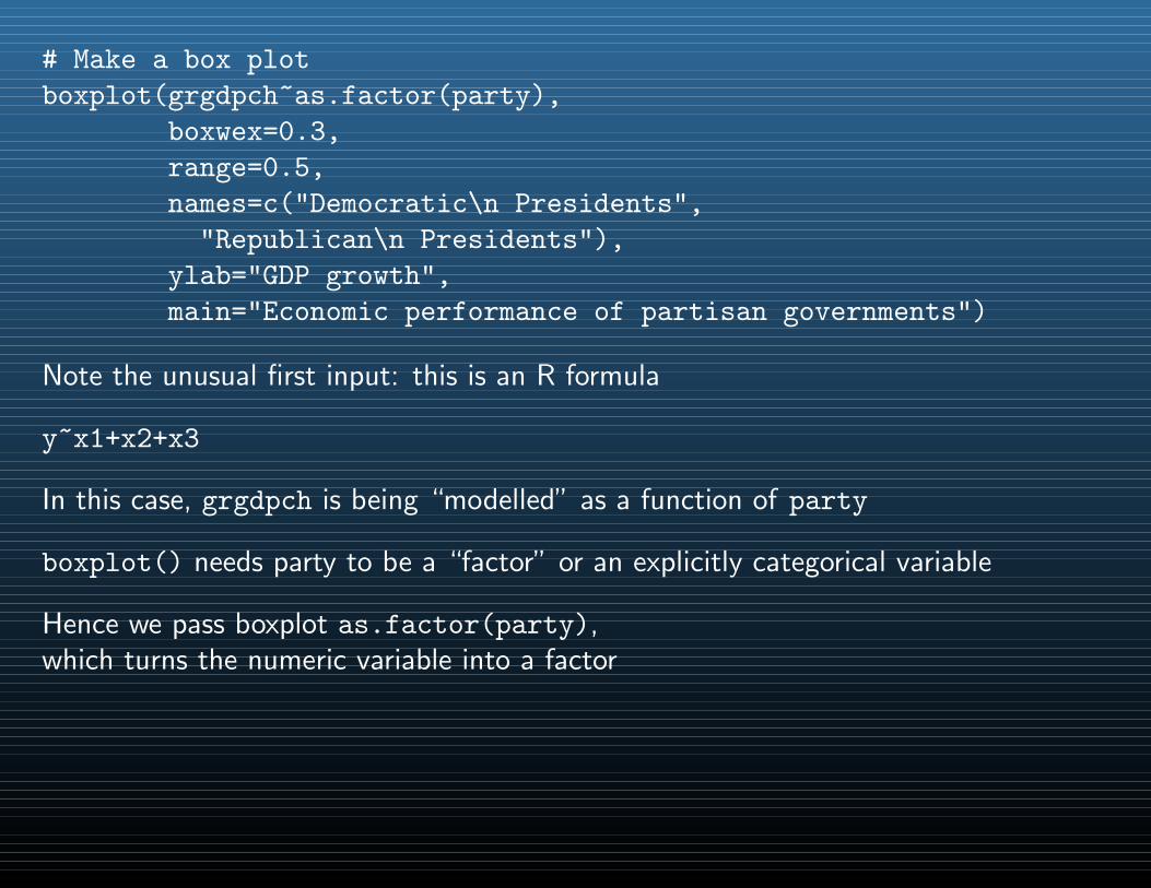
# Make a box plot
boxplot(grgdpch~as.factor(party),
boxwex=0.3,
range=0.5,
names=c("Democratic\n Presidents",
"Republican\n Presidents"),
ylab="GDP growth",
main="Economic performance of partisan governments")
Note the unusual first input: this is an R formula
y~x1+x2+x3
In this case, grgdpch is being “modelled” as a function of party
boxplot() needs party to be a “factor” or an explicitly categorical variable
Hence we pass boxplot as.factor(party),which turns the numeric variable into a factor
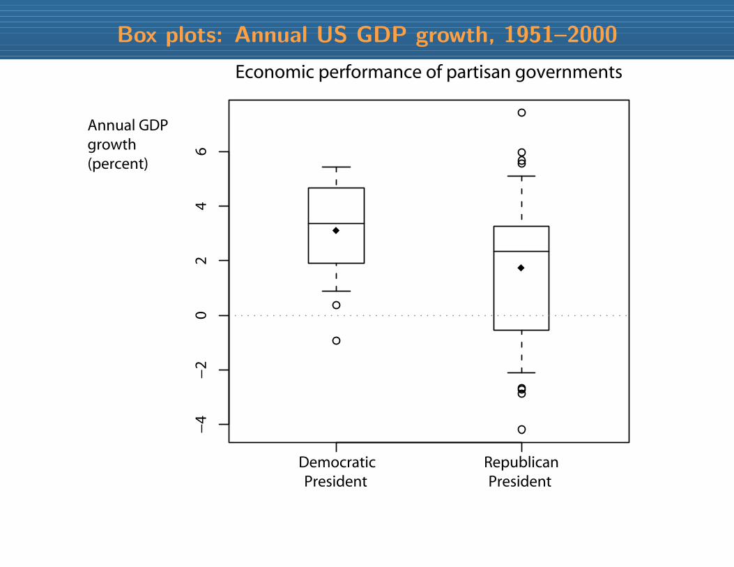
Box plots: Annual US GDP growth, 1951–2000
Democratic President
Republican President
−4
−2
02
46
Economic performance of partisan governments
Annual GDP growth (percent)
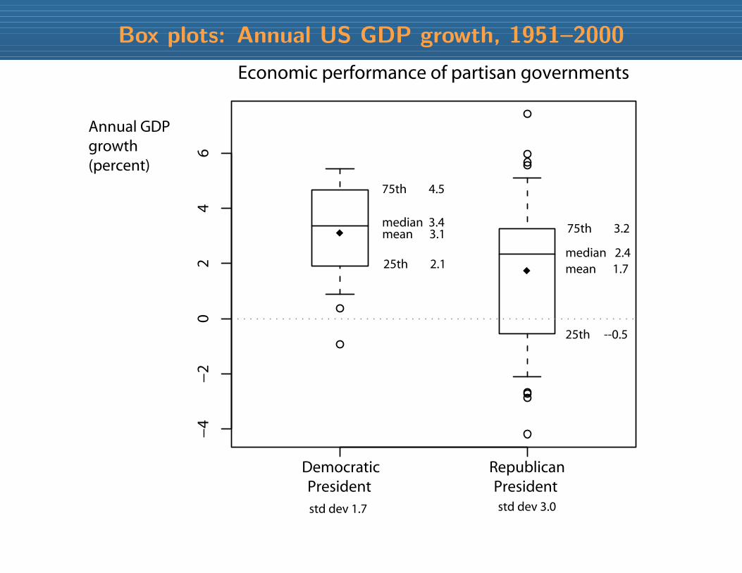
Box plots: Annual US GDP growth, 1951–2000
Democratic President
Republican President
−4
−2
02
46
Economic performance of partisan governments
Annual GDP growth (percent)
mean 3.1
mean 1.7
75th 4.5
25th 2.1median 2.4
75th 3.2
25th --0.5
median 3.4
std dev 1.7 std dev 3.0
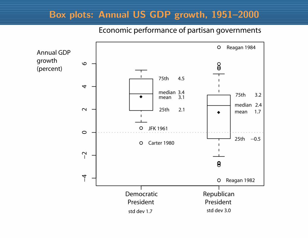
Box plots: Annual US GDP growth, 1951–2000
Democratic President
Republican President
−4
−2
02
46
Economic performance of partisan governments
Annual GDP growth (percent)
Reagan 1984
Reagan 1982
Carter 1980
JFK 1961
mean 3.1
mean 1.7
75th 4.5
25th 2.1median 2.4
75th 3.2
25th --0.5
median 3.4
std dev 1.7 std dev 3.0
Box plots: Annual US GDP growth, 1951–2000
Democratic President
Republican President
−4
−2
02
46
Economic performance of partisan governments
Annual GDP growth (percent)
Reagan 1984
Reagan 1982
Carter 1980
JFK 1961
Help!
To get help on a known command x, type help(x) or ?x
To search the help files using a keyword string s, type help.search(s)
Note that this implies to search on the word regression, you should typehelp.search("regression")
but to get help for the command lm, you should type help(lm)
Hard to use Google directly for R help (“r” is kind of a common letter)
Easiest way to get help from the web: rseek.org
Rseek tries to limit results to R topics (not wholly successful)
Installing R on a PC
• Go to the Comprehensive R Archive Network (CRAN)http://cran.r-project.org/
• Under the heading “Download and Install R”, click on “Download R for Windows”
• Click on “base”
• Download and run the R setup program.The name changes as R gets updated;the current version is “R-3.4.1-win.exe”
• Once you have R running on your computer,you can add new libraries from inside R by selecting“Install packages” from the Packages menu

Installing R on a Mac
• Go to the Comprehensive R Archive Network (CRAN)http://cran.r-project.org/
• Under the heading “Download and Install R”, click on “Download R for MacOSX”
• Download and run the R setup program.The name changes as R gets updated;the current version is “R-3.4.1.pkg”
• Once you have R running on your computer,you can add new libraries from inside R by selecting“Install packages” from the Packages menu

Editing scripts
Don’t use Microsoft Word to edit R code!
Word adds lots of “stuff” to text; R needs the script in a plain text file.
Some text editors:
• Notepad: Free, and comes with Windows (under Start→ Programs→ Accessories).Gets the job done; not powerful.
• TextEdit: Free, and comes with Mac OS X. Gets the job done; not powerful.
• TINN-R: Free and powerful. Windows only.http://www.sciviews.org/Tinn-R/
• Emacs: Free and very powerful (my preference). Can use for R, Latex, and anyother language. Available for Mac, PC, and Linux.
For Mac (easy installation): http://aquamacs.org/
For Windows (see the README): http://ftp.gnu.org/gnu/emacs/windows/
Editing data
R can load many other packages’ data files
See the foreign library for commands
For simplicity & universality, I prefer Comma-Separated Variable (CSV) files
Microsoft Excel can edit and export CSV files (under Save As)
R can read them using read.csv()
OpenOffice free alternative to Excel (for Windows and Unix):http://www.openoffice.org/
My detailed guide to installing social science software on the Mac:http://thewastebook.com/?post=social-science-computing-for-mac
Focus on steps 1.1 and 1.3 for now; come back later for Latex in step 1.2
Example 2: A simple linear regression
Let’s investigate a bivariate relationship
Cross-national data on fertility (children born per adult female) and the percentageof women practicing contraception.
Data are from 50 developing countries.
Source: Robey, B., Shea, M. A., Rutstein, O. and Morris, L. (1992) “Thereproductive revolution: New survey findings.” Population Reports. Technical ReportM-11.
Example 2: A simple linear regression
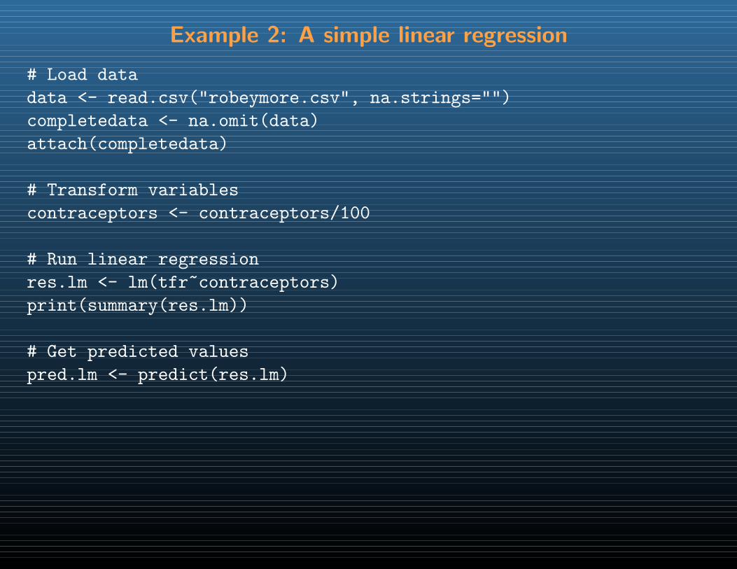
# Load data
data <- read.csv("robeymore.csv", na.strings="")
completedata <- na.omit(data)
attach(completedata)
# Transform variables
contraceptors <- contraceptors/100
# Run linear regression
res.lm <- lm(tfr~contraceptors)
print(summary(res.lm))
# Get predicted values
pred.lm <- predict(res.lm)
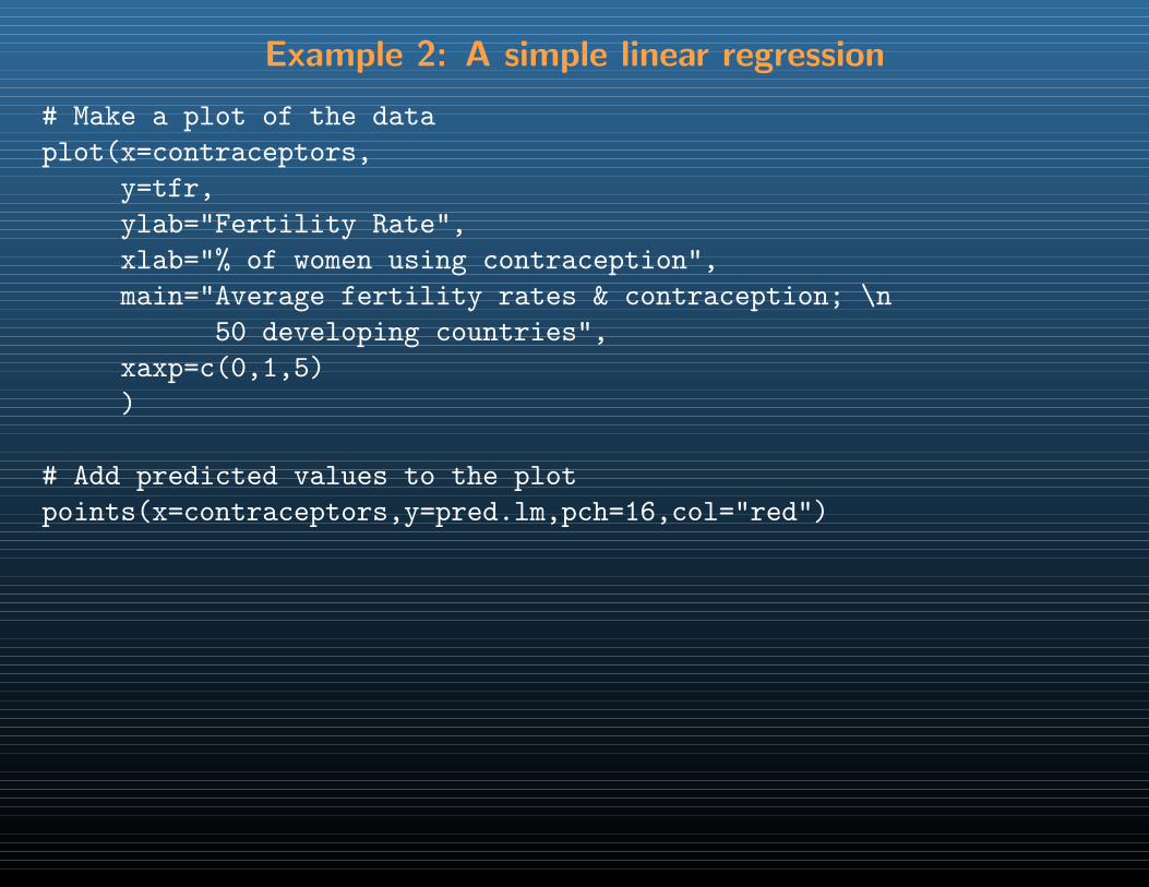
Example 2: A simple linear regression
# Make a plot of the data
plot(x=contraceptors,
y=tfr,
ylab="Fertility Rate",
xlab="% of women using contraception",
main="Average fertility rates & contraception; \n
50 developing countries",
xaxp=c(0,1,5)
)
# Add predicted values to the plot
points(x=contraceptors,y=pred.lm,pch=16,col="red")
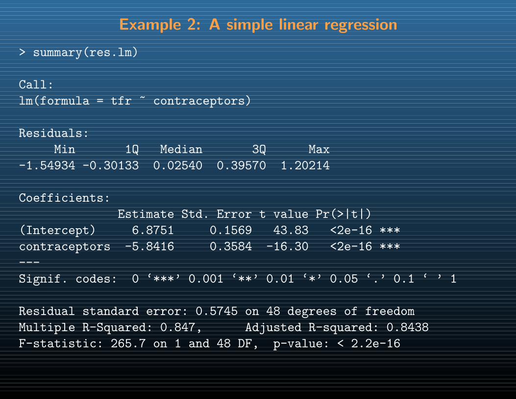
Example 2: A simple linear regression
> summary(res.lm)
Call:
lm(formula = tfr ~ contraceptors)
Residuals:
Min 1Q Median 3Q Max
-1.54934 -0.30133 0.02540 0.39570 1.20214
Coefficients:
Estimate Std. Error t value Pr(>|t|)
(Intercept) 6.8751 0.1569 43.83 <2e-16 ***
contraceptors -5.8416 0.3584 -16.30 <2e-16 ***
---
Signif. codes: 0 ‘***’ 0.001 ‘**’ 0.01 ‘*’ 0.05 ‘.’ 0.1 ‘ ’ 1
Residual standard error: 0.5745 on 48 degrees of freedom
Multiple R-Squared: 0.847, Adjusted R-squared: 0.8438
F-statistic: 265.7 on 1 and 48 DF, p-value: < 2.2e-16
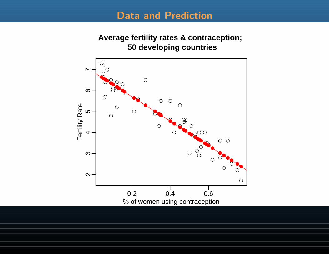
Data and Prediction
0.2 0.4 0.6
23
45
67
Average fertility rates & contraception; 50 developing countries
% of women using contraception
Fer
tility
Rat
e
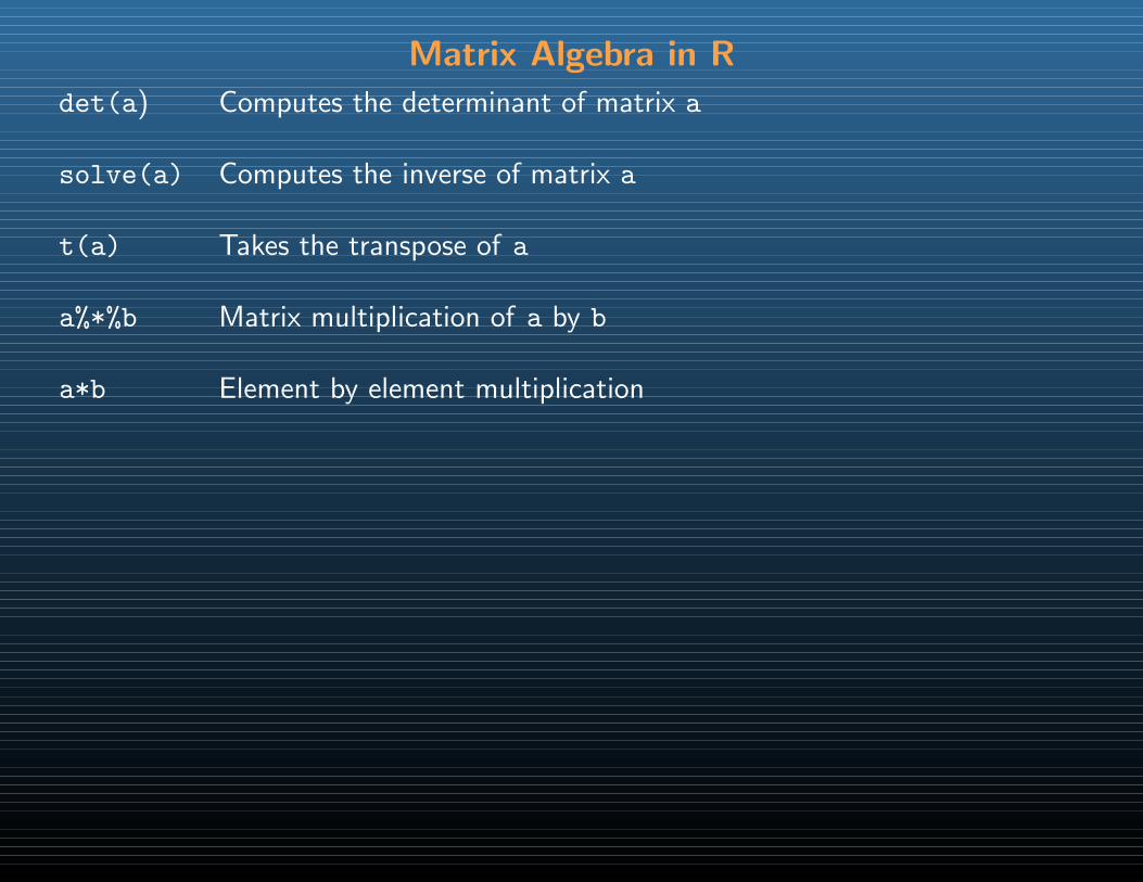
Matrix Algebra in R
det(a) Computes the determinant of matrix a
solve(a) Computes the inverse of matrix a
t(a) Takes the transpose of a
a%*%b Matrix multiplication of a by b
a*b Element by element multiplication
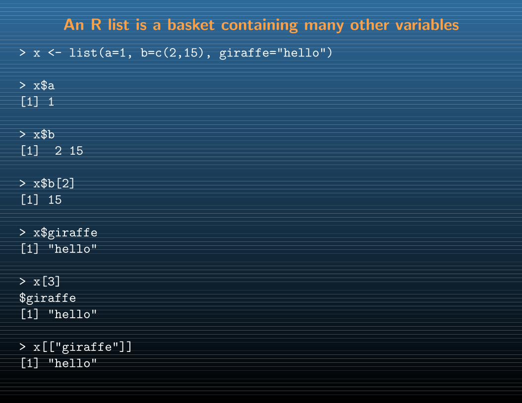
An R list is a basket containing many other variables
> x <- list(a=1, b=c(2,15), giraffe="hello")
> x$a
[1] 1
> x$b
[1] 2 15
> x$b[2]
[1] 15
> x$giraffe
[1] "hello"
> x[3]
$giraffe
[1] "hello"
> x[["giraffe"]]
[1] "hello"
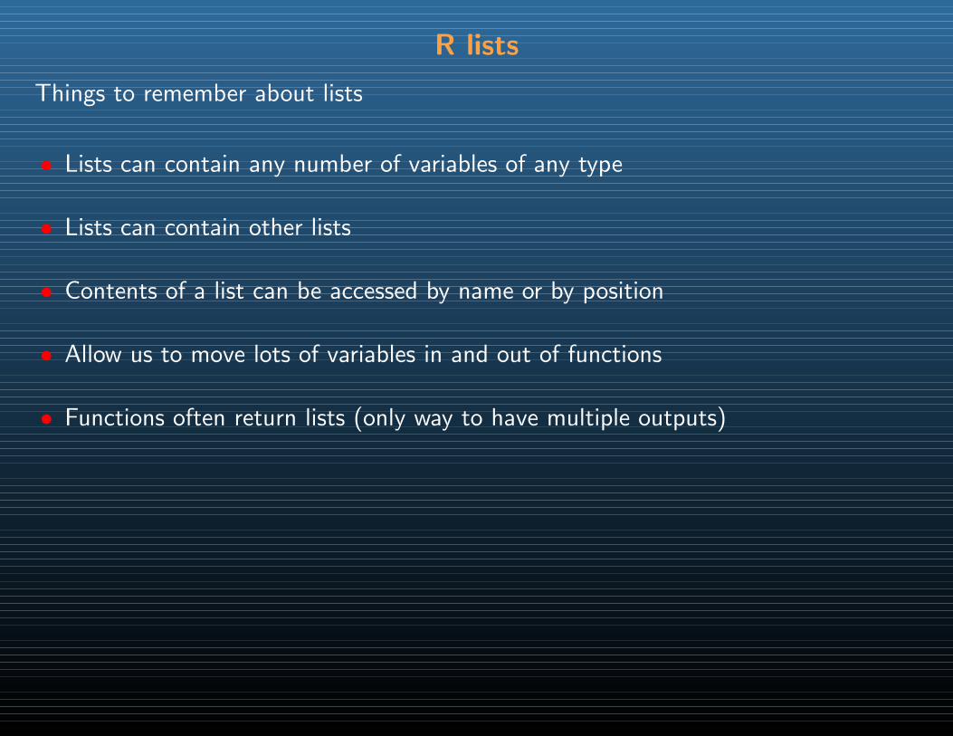
R lists
Things to remember about lists
• Lists can contain any number of variables of any type
• Lists can contain other lists
• Contents of a list can be accessed by name or by position
• Allow us to move lots of variables in and out of functions
• Functions often return lists (only way to have multiple outputs)
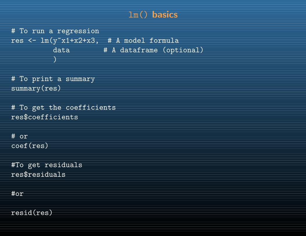
lm() basics
# To run a regression
res <- lm(y~x1+x2+x3, # A model formula
data # A dataframe (optional)
)
# To print a summary
summary(res)
# To get the coefficients
res$coefficients
# or
coef(res)
#To get residuals
res$residuals
#or
resid(res)
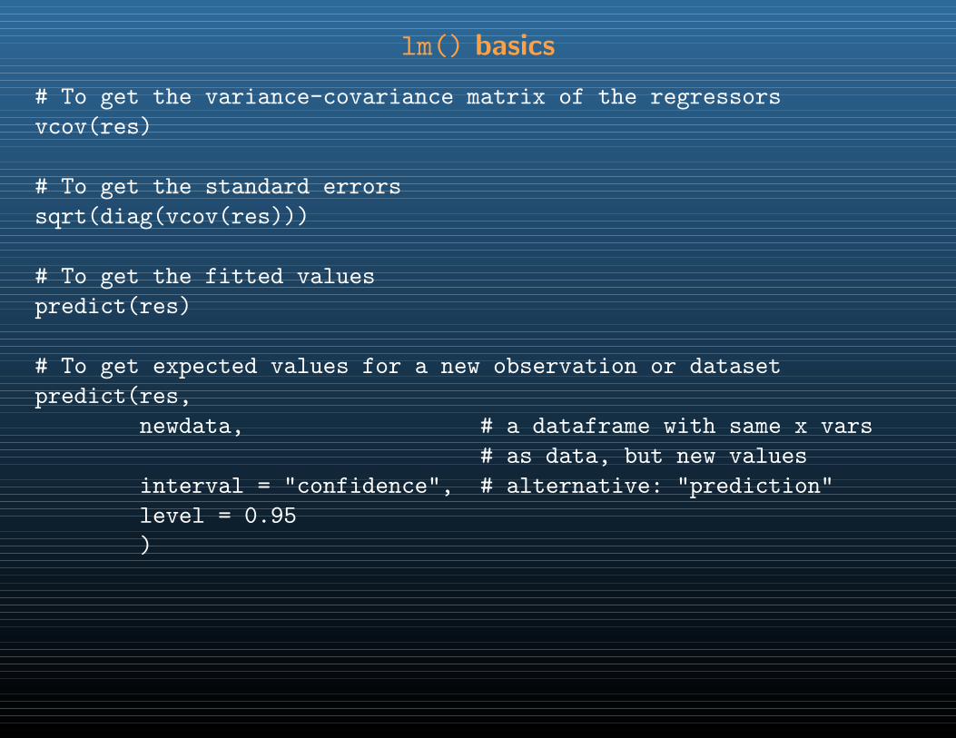
lm() basics
# To get the variance-covariance matrix of the regressors
vcov(res)
# To get the standard errors
sqrt(diag(vcov(res)))
# To get the fitted values
predict(res)
# To get expected values for a new observation or dataset
predict(res,
newdata, # a dataframe with same x vars
# as data, but new values
interval = "confidence", # alternative: "prediction"
level = 0.95
)

R lists & Object Oriented Programming
A list object in R can be given a special “class” using the class() function
This is just a metatag telling other R functions that this list object conforms to acertain format
So when we run a linear regression like this:
res <- lm(y~x1+x2+x3, data)
The result res is a list object of class ‘‘lm’’
Other functions like plot() and predict() will react to res in a special waybecause of this class designation
Specifically, they will run functions called plot.lm() and predict.lm()
Object-oriented programming:a function does different things depending on class of input object
Example 3: Party systems & Redistribution
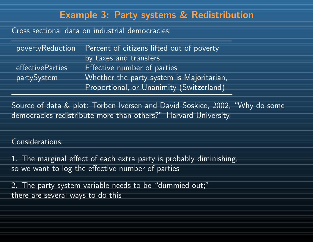
Example 3: Party systems & Redistribution
Cross sectional data on industrial democracies:
povertyReduction Percent of citizens lifted out of povertyby taxes and transfers
effectiveParties Effective number of partiespartySystem Whether the party system is Majoritarian,
Proportional, or Unanimity (Switzerland)
Source of data & plot: Torben Iversen and David Soskice, 2002, “Why do somedemocracies redistribute more than others?” Harvard University.
Considerations:
1. The marginal effect of each extra party is probably diminishing,so we want to log the effective number of parties
2. The party system variable needs to be “dummied out;”there are several ways to do this
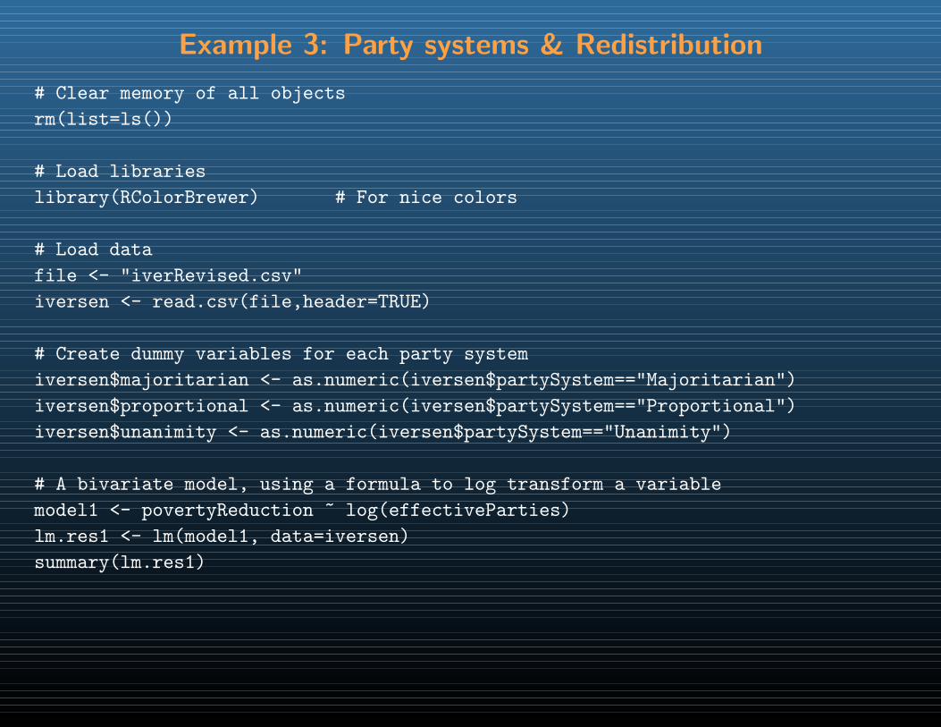
Example 3: Party systems & Redistribution
# Clear memory of all objects
rm(list=ls())
# Load libraries
library(RColorBrewer) # For nice colors
# Load data
file <- "iverRevised.csv"
iversen <- read.csv(file,header=TRUE)
# Create dummy variables for each party system
iversen$majoritarian <- as.numeric(iversen$partySystem=="Majoritarian")
iversen$proportional <- as.numeric(iversen$partySystem=="Proportional")
iversen$unanimity <- as.numeric(iversen$partySystem=="Unanimity")
# A bivariate model, using a formula to log transform a variable
model1 <- povertyReduction ~ log(effectiveParties)
lm.res1 <- lm(model1, data=iversen)
summary(lm.res1)
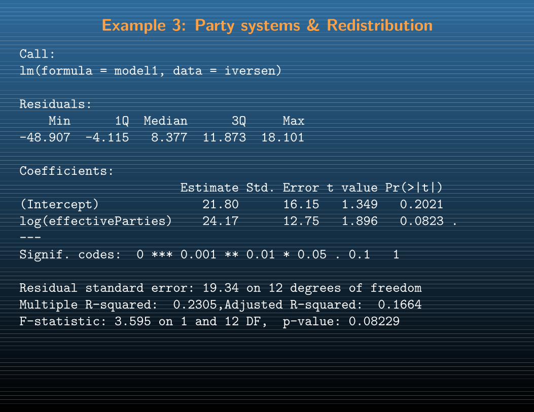
Example 3: Party systems & Redistribution
Call:
lm(formula = model1, data = iversen)
Residuals:
Min 1Q Median 3Q Max
-48.907 -4.115 8.377 11.873 18.101
Coefficients:
Estimate Std. Error t value Pr(>|t|)
(Intercept) 21.80 16.15 1.349 0.2021
log(effectiveParties) 24.17 12.75 1.896 0.0823 .
---
Signif. codes: 0 *** 0.001 ** 0.01 * 0.05 . 0.1 1
Residual standard error: 19.34 on 12 degrees of freedom
Multiple R-squared: 0.2305,Adjusted R-squared: 0.1664
F-statistic: 3.595 on 1 and 12 DF, p-value: 0.08229
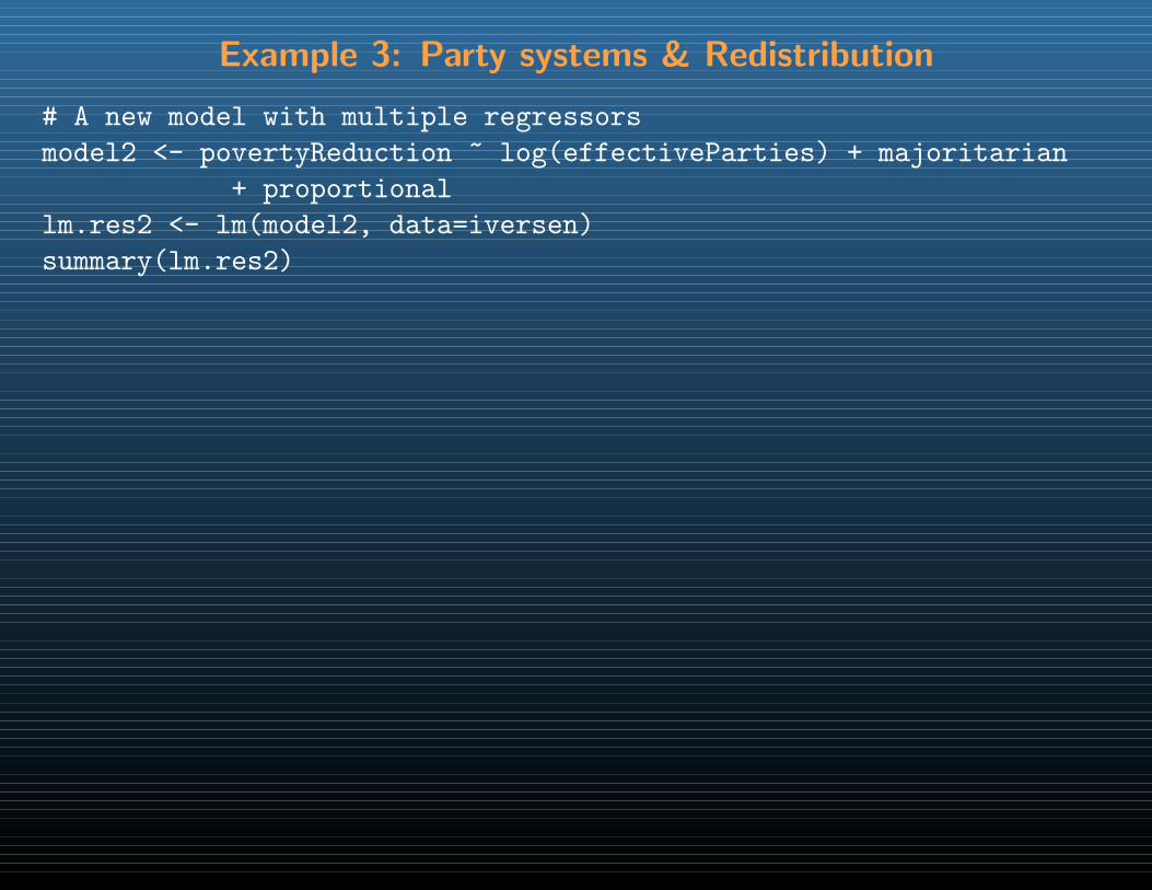
Example 3: Party systems & Redistribution
# A new model with multiple regressors
model2 <- povertyReduction ~ log(effectiveParties) + majoritarian
+ proportional
lm.res2 <- lm(model2, data=iversen)
summary(lm.res2)
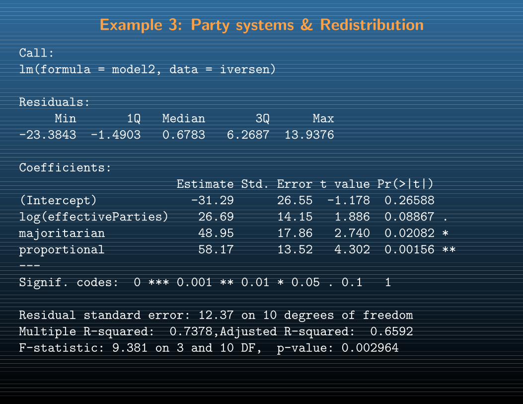
Example 3: Party systems & Redistribution
Call:
lm(formula = model2, data = iversen)
Residuals:
Min 1Q Median 3Q Max
-23.3843 -1.4903 0.6783 6.2687 13.9376
Coefficients:
Estimate Std. Error t value Pr(>|t|)
(Intercept) -31.29 26.55 -1.178 0.26588
log(effectiveParties) 26.69 14.15 1.886 0.08867 .
majoritarian 48.95 17.86 2.740 0.02082 *
proportional 58.17 13.52 4.302 0.00156 **
---
Signif. codes: 0 *** 0.001 ** 0.01 * 0.05 . 0.1 1
Residual standard error: 12.37 on 10 degrees of freedom
Multiple R-squared: 0.7378,Adjusted R-squared: 0.6592
F-statistic: 9.381 on 3 and 10 DF, p-value: 0.002964
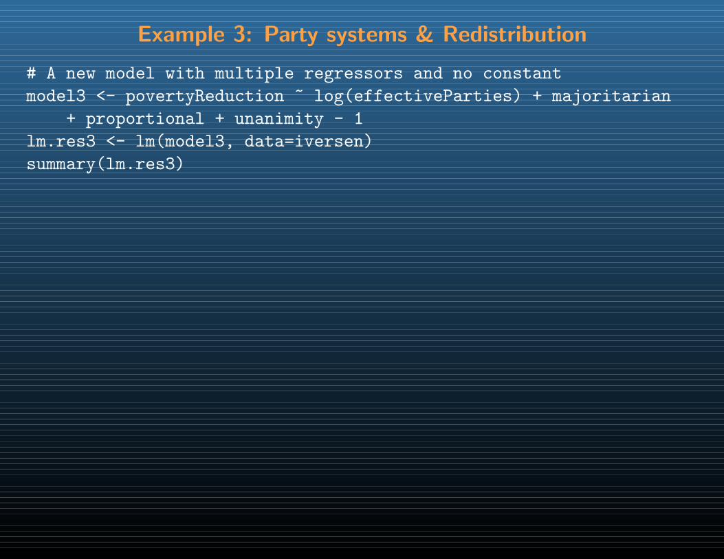
Example 3: Party systems & Redistribution
# A new model with multiple regressors and no constant
model3 <- povertyReduction ~ log(effectiveParties) + majoritarian
+ proportional + unanimity - 1
lm.res3 <- lm(model3, data=iversen)
summary(lm.res3)
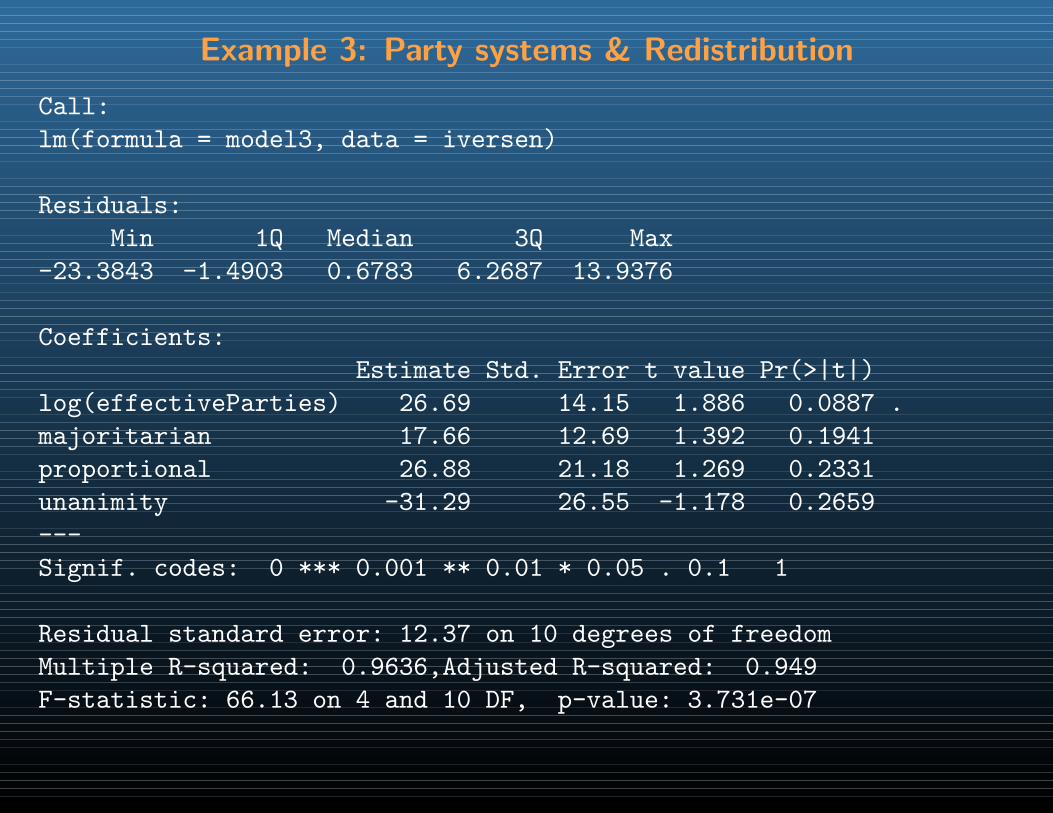
Example 3: Party systems & Redistribution
Call:
lm(formula = model3, data = iversen)
Residuals:
Min 1Q Median 3Q Max
-23.3843 -1.4903 0.6783 6.2687 13.9376
Coefficients:
Estimate Std. Error t value Pr(>|t|)
log(effectiveParties) 26.69 14.15 1.886 0.0887 .
majoritarian 17.66 12.69 1.392 0.1941
proportional 26.88 21.18 1.269 0.2331
unanimity -31.29 26.55 -1.178 0.2659
---
Signif. codes: 0 *** 0.001 ** 0.01 * 0.05 . 0.1 1
Residual standard error: 12.37 on 10 degrees of freedom
Multiple R-squared: 0.9636,Adjusted R-squared: 0.949
F-statistic: 66.13 on 4 and 10 DF, p-value: 3.731e-07
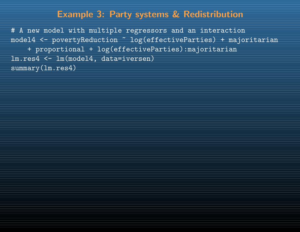
Example 3: Party systems & Redistribution
# A new model with multiple regressors and an interaction
model4 <- povertyReduction ~ log(effectiveParties) + majoritarian
+ proportional + log(effectiveParties):majoritarian
lm.res4 <- lm(model4, data=iversen)
summary(lm.res4)
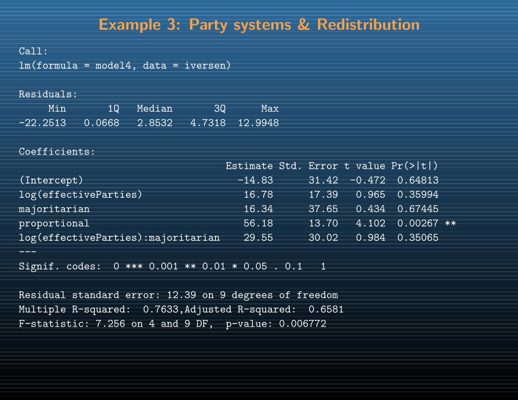
Example 3: Party systems & Redistribution
Call:
lm(formula = model4, data = iversen)
Residuals:
Min 1Q Median 3Q Max
-22.2513 0.0668 2.8532 4.7318 12.9948
Coefficients:
Estimate Std. Error t value Pr(>|t|)
(Intercept) -14.83 31.42 -0.472 0.64813
log(effectiveParties) 16.78 17.39 0.965 0.35994
majoritarian 16.34 37.65 0.434 0.67445
proportional 56.18 13.70 4.102 0.00267 **
log(effectiveParties):majoritarian 29.55 30.02 0.984 0.35065
---
Signif. codes: 0 *** 0.001 ** 0.01 * 0.05 . 0.1 1
Residual standard error: 12.39 on 9 degrees of freedom
Multiple R-squared: 0.7633,Adjusted R-squared: 0.6581
F-statistic: 7.256 on 4 and 9 DF, p-value: 0.006772
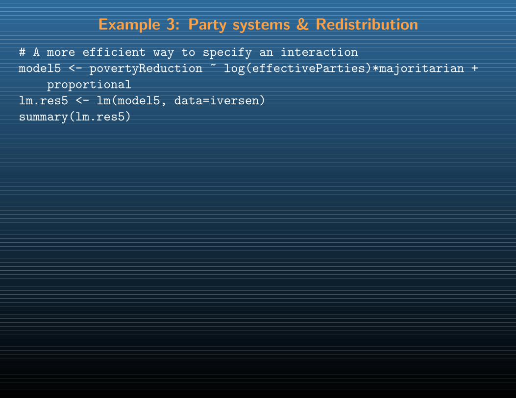
Example 3: Party systems & Redistribution
# A more efficient way to specify an interaction
model5 <- povertyReduction ~ log(effectiveParties)*majoritarian +
proportional
lm.res5 <- lm(model5, data=iversen)
summary(lm.res5)
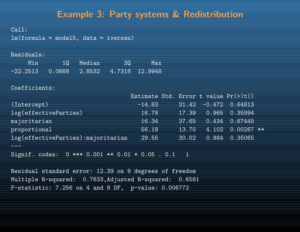
Example 3: Party systems & Redistribution
Call:
lm(formula = model5, data = iversen)
Residuals:
Min 1Q Median 3Q Max
-22.2513 0.0668 2.8532 4.7318 12.9948
Coefficients:
Estimate Std. Error t value Pr(>|t|)
(Intercept) -14.83 31.42 -0.472 0.64813
log(effectiveParties) 16.78 17.39 0.965 0.35994
majoritarian 16.34 37.65 0.434 0.67445
proportional 56.18 13.70 4.102 0.00267 **
log(effectiveParties):majoritarian 29.55 30.02 0.984 0.35065
---
Signif. codes: 0 *** 0.001 ** 0.01 * 0.05 . 0.1 1
Residual standard error: 12.39 on 9 degrees of freedom
Multiple R-squared: 0.7633,Adjusted R-squared: 0.6581
F-statistic: 7.256 on 4 and 9 DF, p-value: 0.006772
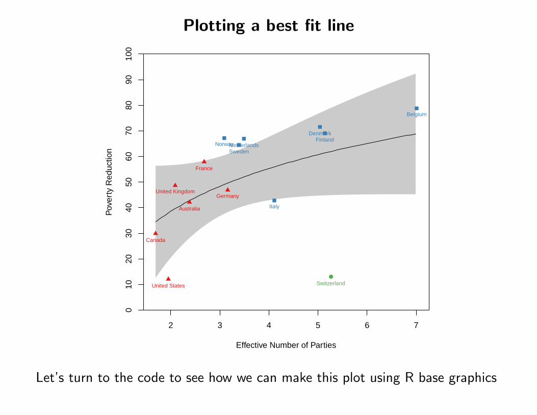
Plotting a best fit line
2 3 4 5 6 7
010
2030
4050
6070
8090
100
Effective Number of Parties
Pov
erty
Red
uctio
n
Australia
Canada
France
GermanyUnited Kingdom
United States
Belgium
DenmarkFinland
Italy
NetherlandsNorwaySweden
Switzerland
Let’s turn to the code to see how we can make this plot using R base graphics
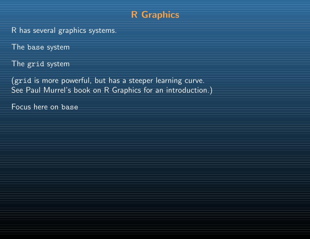
R Graphics
R has several graphics systems.
The base system
The grid system
(grid is more powerful, but has a steeper learning curve.See Paul Murrel’s book on R Graphics for an introduction.)
Focus here on base

R Graphics: Devices
Everything you draw in R must be drawn on a canvas
Must create the canvas before you draw anything
Computer canvasses are devices you draw to
Devices save graphical input in different ways
Sometimes to the disk, sometimes to the screen
Most important distinction: raster vs. vector devices

Vector vs. raster
Pointalism = raster graphics. Plot each pixel on an n by m grid.

Vector vs. rasterPixel = Point = Raster
Good for pictures. Bad for drawings/graphics/cartoons.
(Puzzle: isn’t everything raster? In display, yes. Not in storage)
Advantages of vector:
• Easily manipulable/modifiable groupings of objects
• Easy to scale objects larger or smaller/ Arbitrary precision
• Much smaller file sizes
• Can always convert to raster (but not the other way round, at least not well)
Disadvantages:
• A photograph would be really hard to show (and huge file size)
• Not web accessible. Convert to PNG or PDF.
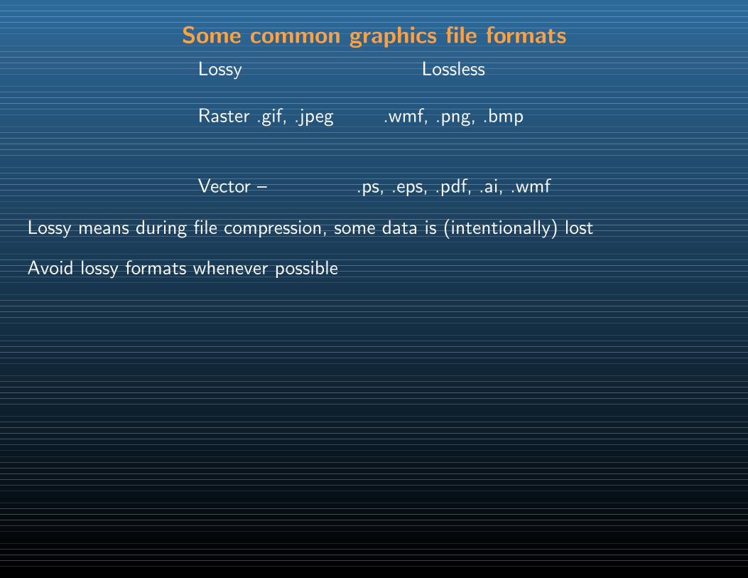
Some common graphics file formats
Lossy Lossless
Raster .gif, .jpeg .wmf, .png, .bmp
Vector – .ps, .eps, .pdf, .ai, .wmf
Lossy means during file compression, some data is (intentionally) lost
Avoid lossy formats whenever possible

Some common graphics file formats
In R, have access to several formats:
win.metafile() wmf, Windows media filepdf() pdf, Adobe portable data filepostscript() postscript file (printer language)
quartz() opens a screen; Mac onlywindows() opens a screen; PC onlyx11() opens a screen; works on all machines
Latex, Mac or Unix users can’t use wmf
windows(record=TRUE) let’s you cycle thru old graphs with arrow keys

High-level graphics commands
In R, High level graphics commands:
• produce a standard graphic type
• fill in lots of details (axes, titles, annotation)
• have many configurable parameters
• have varied flexibility
You don’t need to use HLCs to make R graphics.
Could use primitive commands to do each task above
Using low levels commands gives more control but takes more time

Some major high-level graphics commands
Graphic Base command Lattice commandscatterplot plot() xyplot()line plot plot(. . . ,type=”l”) xyplot(. . . ,type=”l”)Bar chart barplot() barchart()Histogram hist() histogram()Smoothed histograms plot() after density() densityplot()boxplot boxplot() bwplot()Dot plot dotchart() dotplot()Contour plots contour() contourplot()image plot image() levelplot()3D surface persp() wireframe()3D scatter scatterplot3d()* cloud()conditional plots coplot() xyplot()Scatterplot matrix splom()Parallel coordinates parallel()Star plot stars()Stem-and-leaf plots stem()ternary plot ternaryplot() in vcdFourfold plot fourfoldplot() in vcdMosaic plots mosaicplot() in vcd
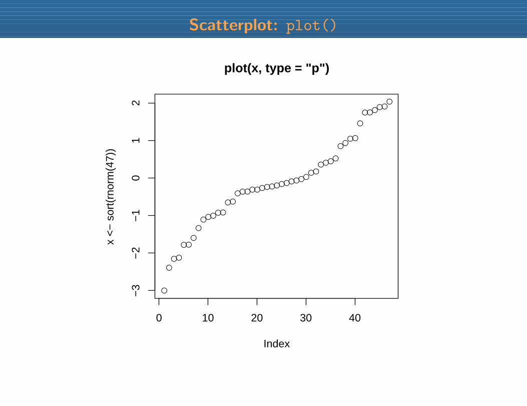
Scatterplot: plot()
0 10 20 30 40
−3
−2
−1
01
2
plot(x, type = "p")
Index
x <
− s
ort(
rnor
m(4
7))
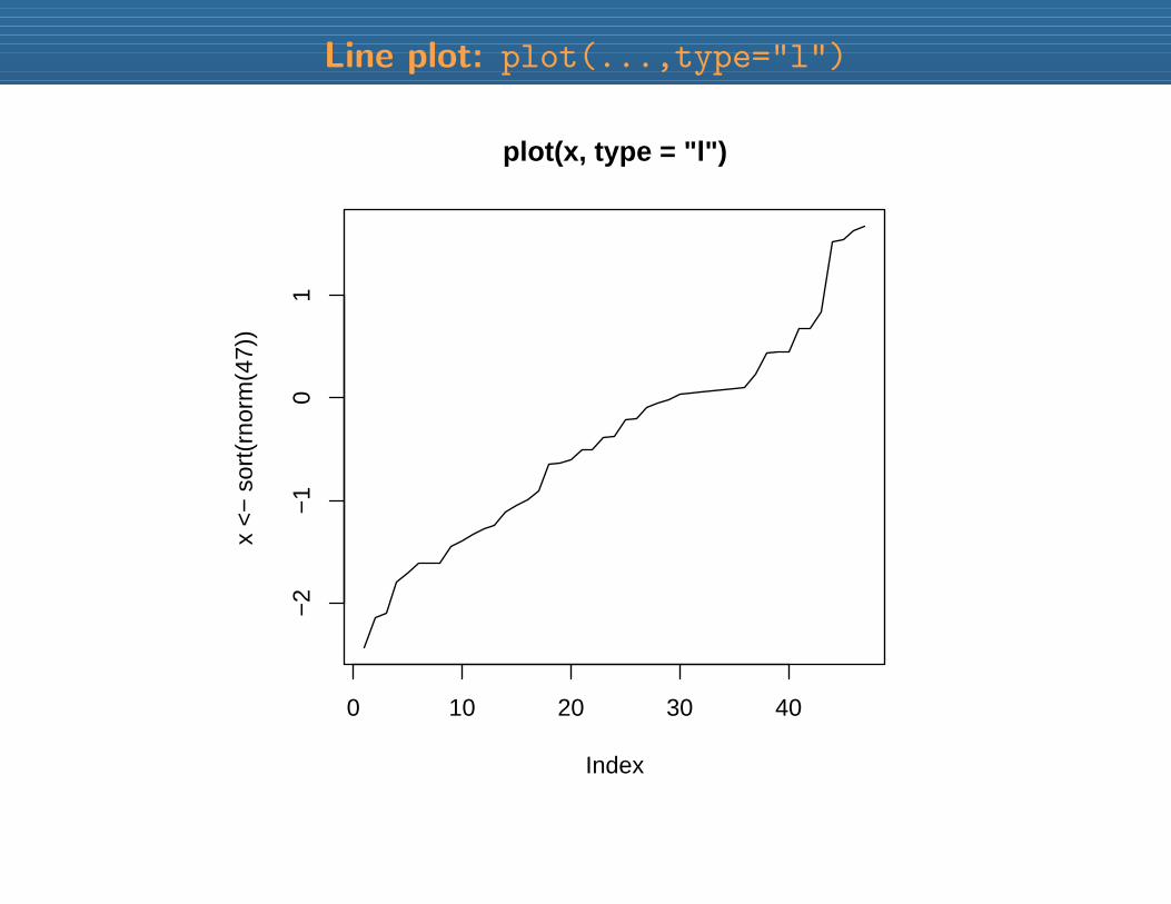
Line plot: plot(...,type="l")
0 10 20 30 40
−2
−1
01
plot(x, type = "l")
Index
x <
− s
ort(
rnor
m(4
7))
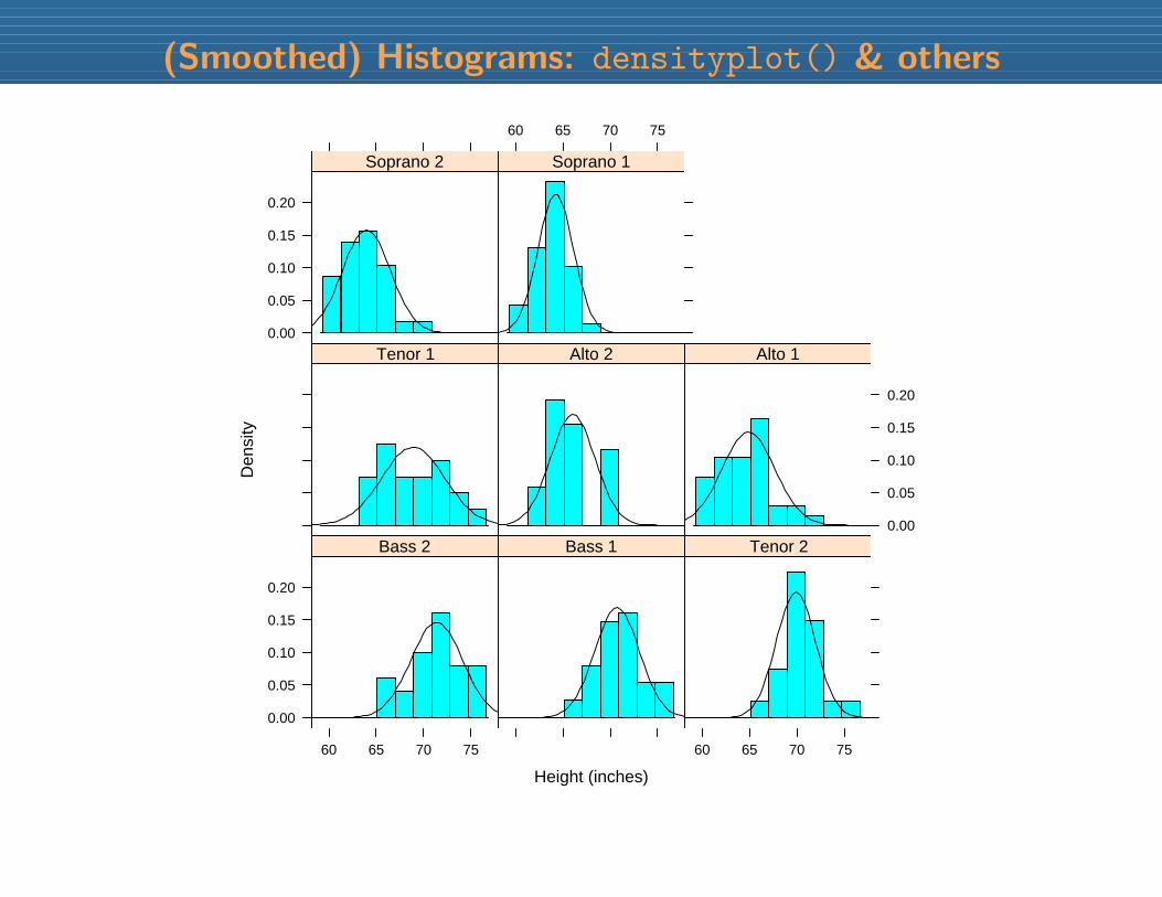
(Smoothed) Histograms: densityplot() & others
Height (inches)
Den
sity
60 65 70 75
0.00
0.05
0.10
0.15
0.20
Bass 2 Bass 1
60 65 70 75
Tenor 2
Tenor 1 Alto 2
0.00
0.05
0.10
0.15
0.20
Alto 10.00
0.05
0.10
0.15
0.20
Soprano 2
60 65 70 75
Soprano 1
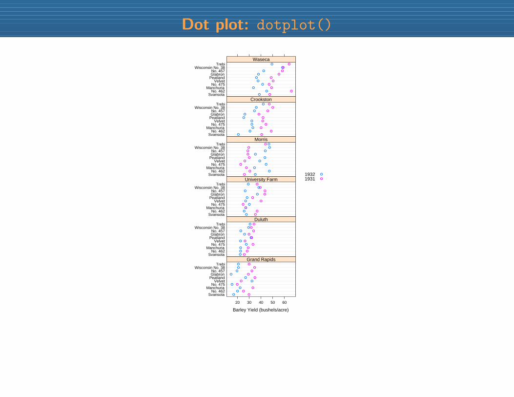
Dot plot: dotplot()
Barley Yield (bushels/acre)
20 30 40 50 60
SvansotaNo. 462
ManchuriaNo. 475
VelvetPeatlandGlabronNo. 457
Wisconsin No. 38Trebi
Grand RapidsSvansota
No. 462Manchuria
No. 475Velvet
PeatlandGlabronNo. 457
Wisconsin No. 38Trebi
DuluthSvansota
No. 462Manchuria
No. 475Velvet
PeatlandGlabronNo. 457
Wisconsin No. 38Trebi
University FarmSvansota
No. 462Manchuria
No. 475Velvet
PeatlandGlabronNo. 457
Wisconsin No. 38Trebi
MorrisSvansota
No. 462Manchuria
No. 475Velvet
PeatlandGlabronNo. 457
Wisconsin No. 38Trebi
CrookstonSvansota
No. 462Manchuria
No. 475Velvet
PeatlandGlabronNo. 457
Wisconsin No. 38Trebi
Waseca
19321931
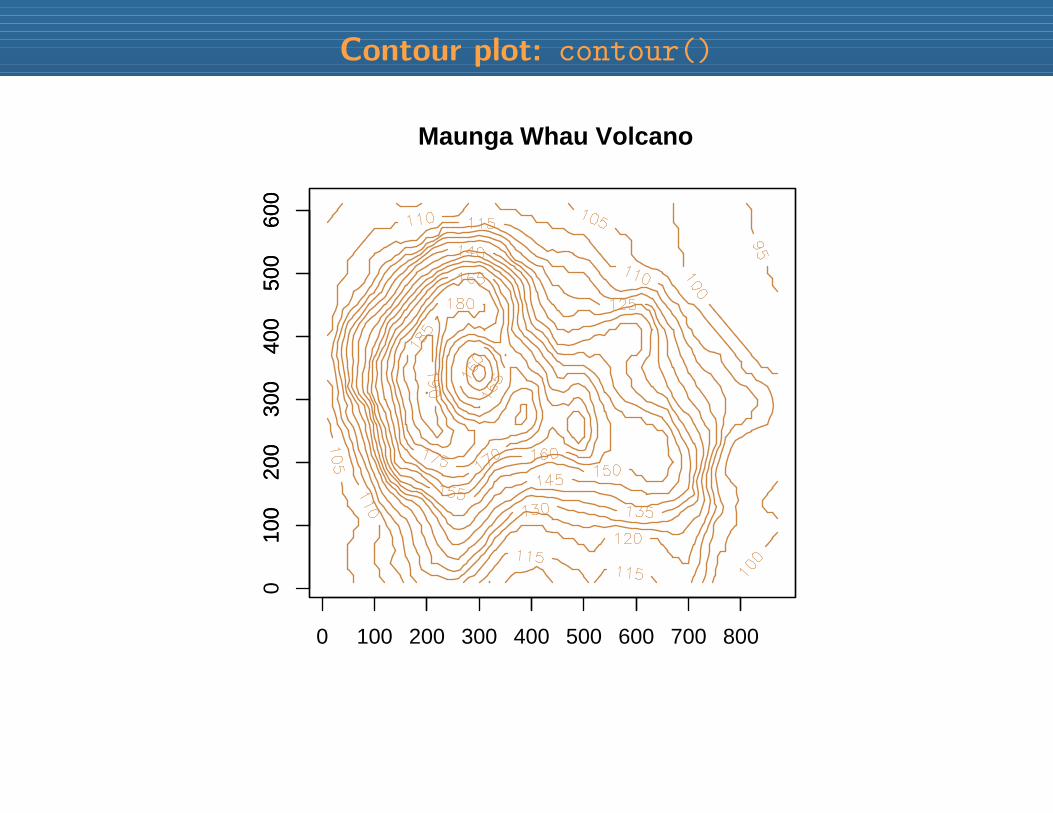
Contour plot: contour()
0 200 400 600 800
010
020
030
040
050
060
0
100 300 500 700
100
200
300
400
500
600
Maunga Whau Volcano
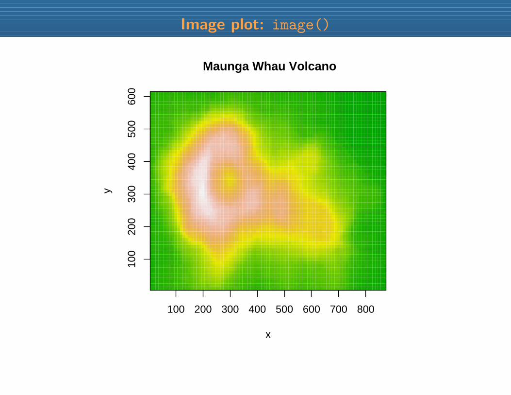
Image plot: image()
x
y
100 200 300 400 500 600 700 800
100
200
300
400
500
600
Maunga Whau Volcano
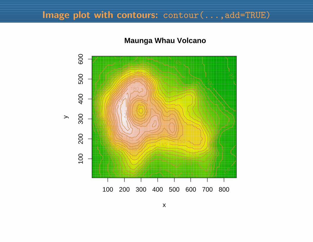
Image plot with contours: contour(...,add=TRUE)
x
y
100 200 300 400 500 600 700 800
100
200
300
400
500
600
Maunga Whau Volcano
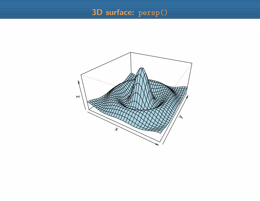
3D surface: persp()
x
yz
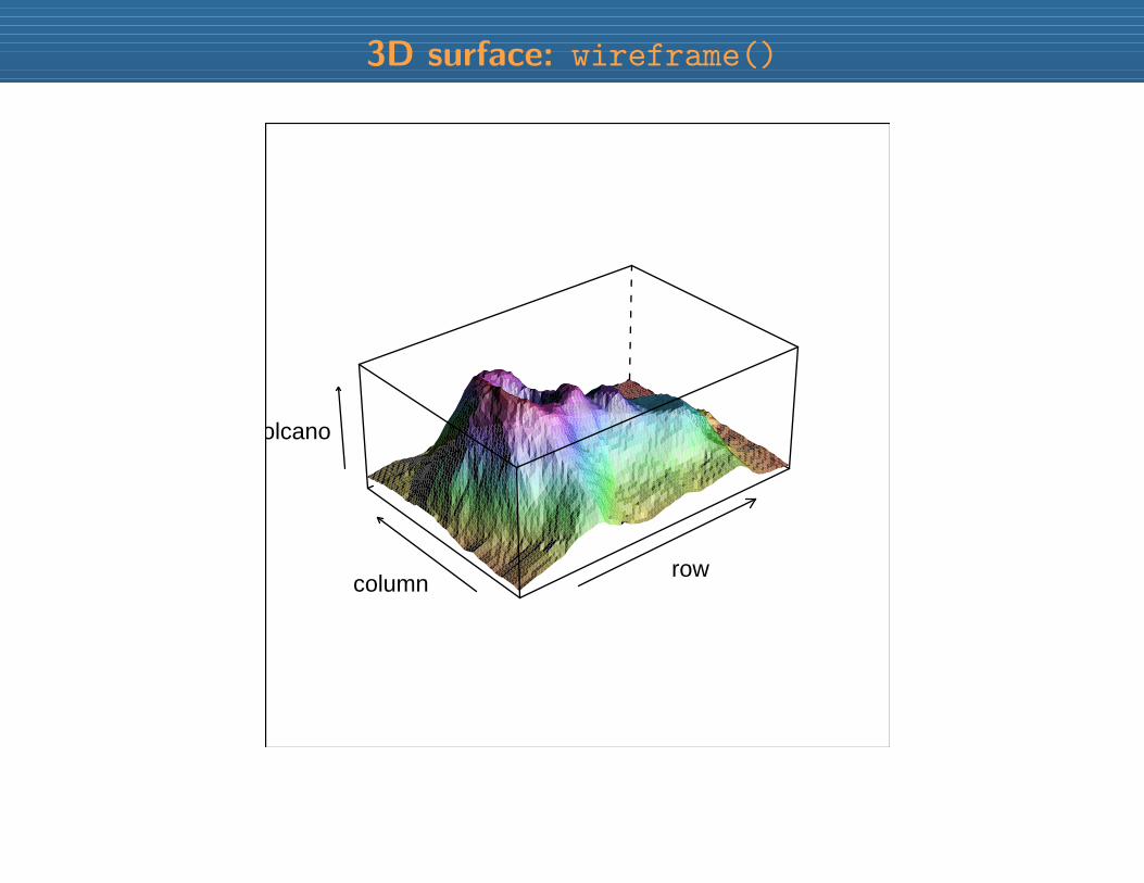
3D surface: wireframe()
rowcolumn
volcano
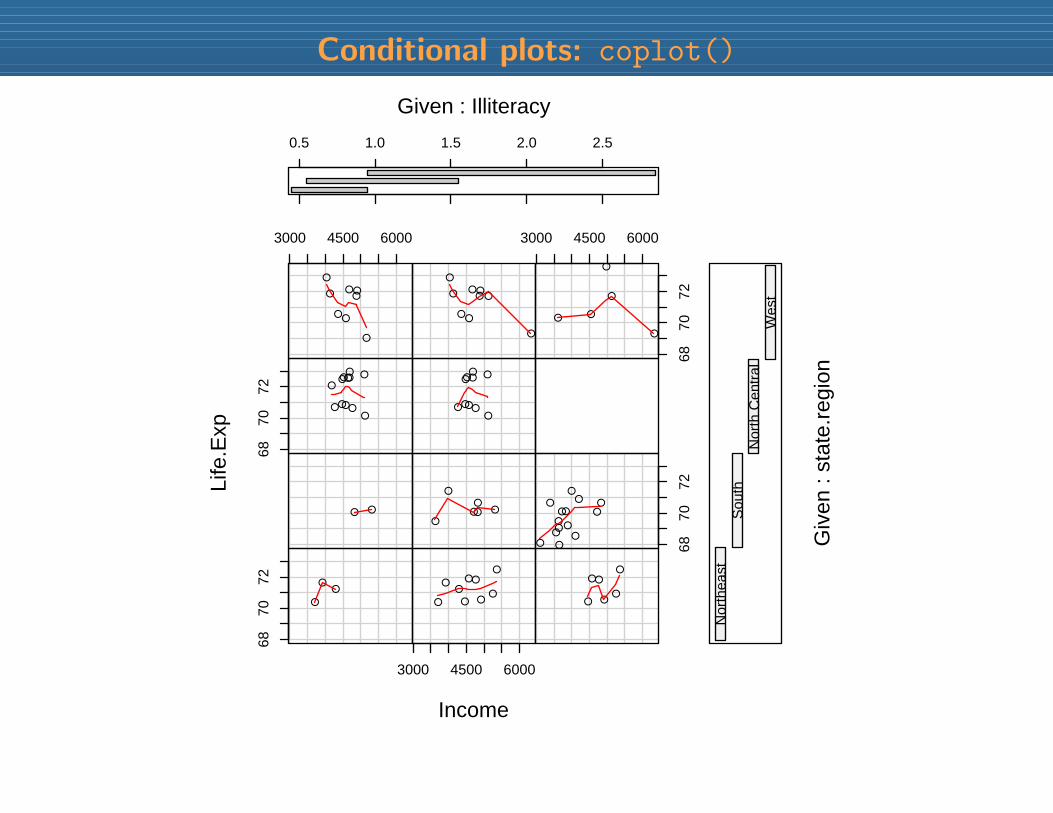
Conditional plots: coplot()
6870
72
3000 4500 6000
6870
72
6870
72
3000 4500 6000
3000 4500 6000
6870
72
Income
Life
.Exp
0.5 1.0 1.5 2.0 2.5
Given : Illiteracy
Nor
thea
stS
outh
Nor
th C
entr
alW
est
Giv
en :
stat
e.re
gion
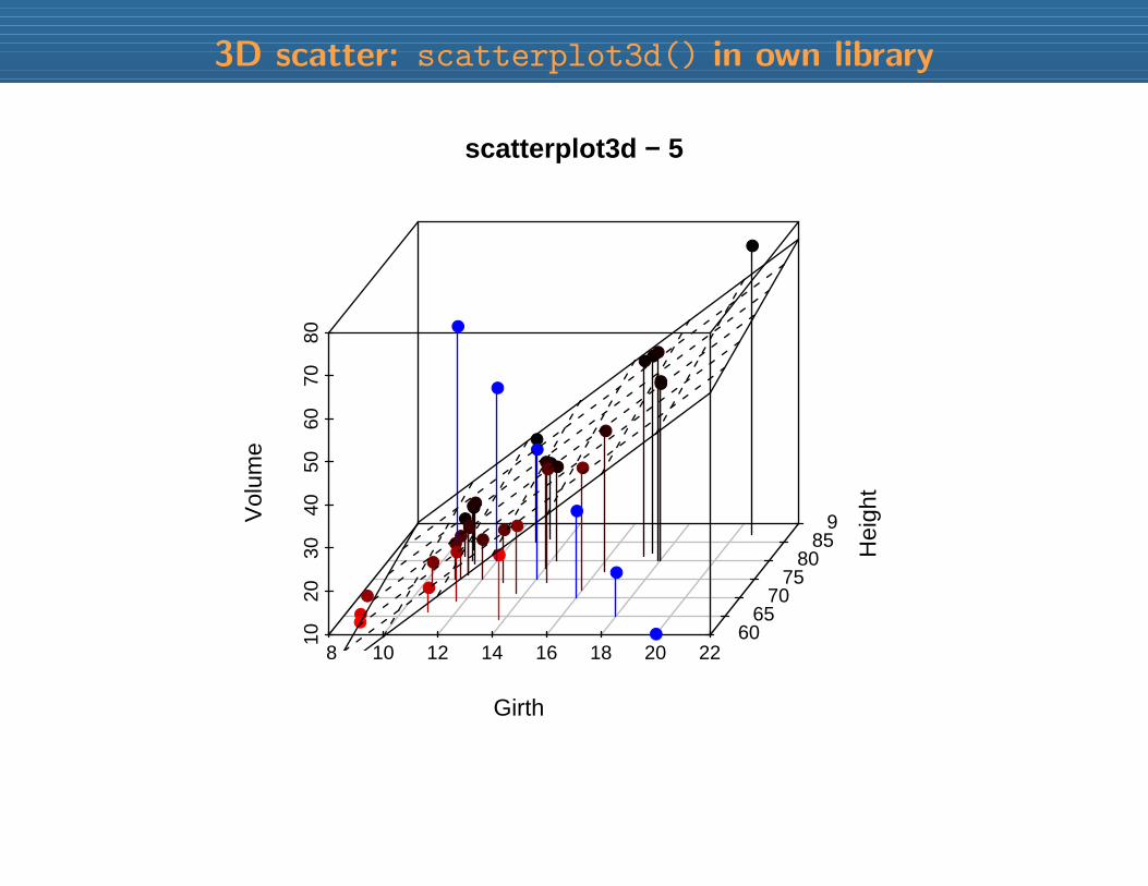
3D scatter: scatterplot3d() in own library
scatterplot3d − 5
8 10 12 14 16 18 20 22
1020
3040
5060
7080
6065
7075
8085
90
Girth
Hei
ght
Vol
ume
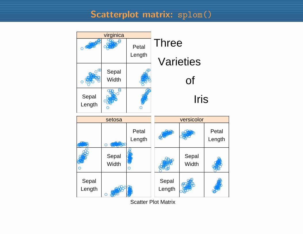
Scatterplot matrix: splom()
Scatter Plot Matrix
SepalLength
SepalWidth
PetalLength
setosa
SepalLength
SepalWidth
Petal
Length
versicolor
SepalLength
SepalWidth
PetalLength
virginica
Three
Varieties
of
Iris
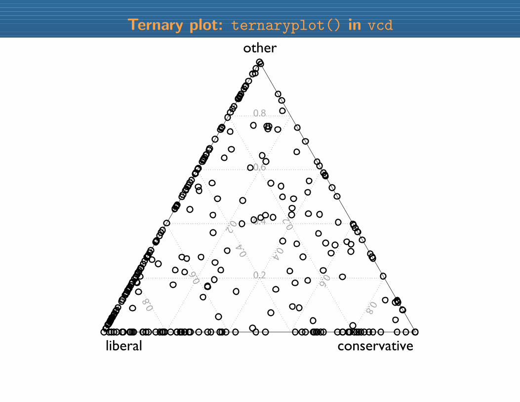
Ternary plot: ternaryplot() in vcd
liberal conservative
other
0.2
0.8
0.2
0.4
0.6
0.4
0.6
0.4
0.6
0.8
0.2
0.8
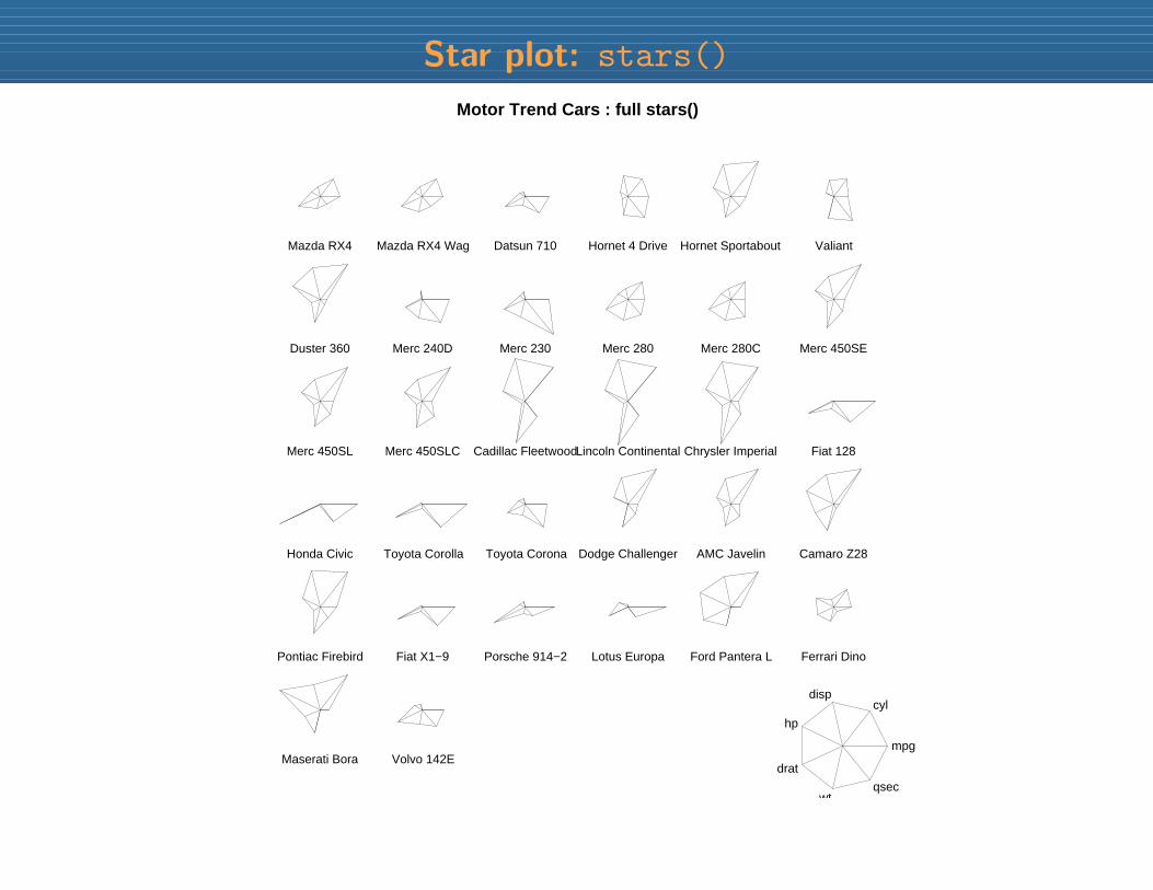
Star plot: stars()
Motor Trend Cars : full stars()
Mazda RX4 Mazda RX4 Wag Datsun 710 Hornet 4 Drive Hornet Sportabout Valiant
Duster 360 Merc 240D Merc 230 Merc 280 Merc 280C Merc 450SE
Merc 450SL Merc 450SLC Cadillac FleetwoodLincoln Continental Chrysler Imperial Fiat 128
Honda Civic Toyota Corolla Toyota Corona Dodge Challenger AMC Javelin Camaro Z28
Pontiac Firebird Fiat X1−9 Porsche 914−2 Lotus Europa Ford Pantera L Ferrari Dino
Maserati Bora Volvo 142Empg
cyldisp
hp
drat
wtqsec
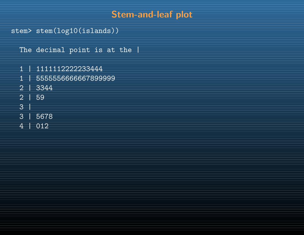
Stem-and-leaf plot
stem> stem(log10(islands))
The decimal point is at the |
1 | 1111112222233444
1 | 5555556666667899999
2 | 3344
2 | 59
3 |
3 | 5678
4 | 012
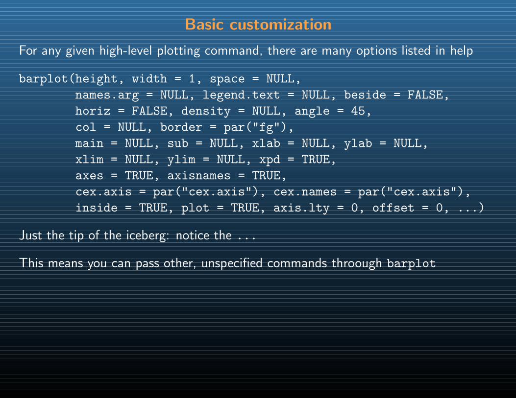
Basic customization
For any given high-level plotting command, there are many options listed in help
barplot(height, width = 1, space = NULL,
names.arg = NULL, legend.text = NULL, beside = FALSE,
horiz = FALSE, density = NULL, angle = 45,
col = NULL, border = par("fg"),
main = NULL, sub = NULL, xlab = NULL, ylab = NULL,
xlim = NULL, ylim = NULL, xpd = TRUE,
axes = TRUE, axisnames = TRUE,
cex.axis = par("cex.axis"), cex.names = par("cex.axis"),
inside = TRUE, plot = TRUE, axis.lty = 0, offset = 0, ...)
Just the tip of the iceberg: notice the ...
This means you can pass other, unspecified commands throough barplot
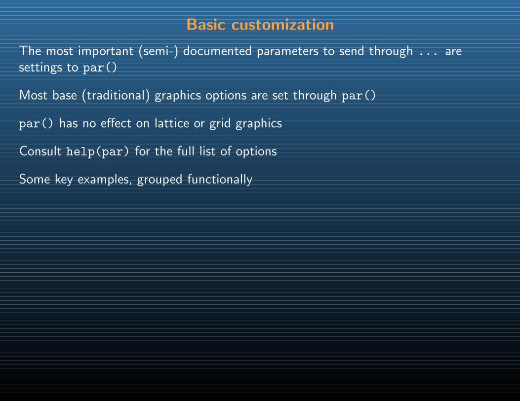
Basic customization
The most important (semi-) documented parameters to send through ... aresettings to par()
Most base (traditional) graphics options are set through par()
par() has no effect on lattice or grid graphics
Consult help(par) for the full list of options
Some key examples, grouped functionally
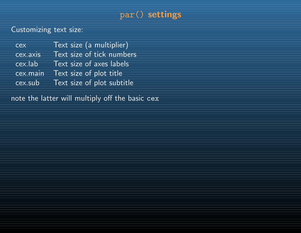
par() settings
Customizing text size:
cex Text size (a multiplier)cex.axis Text size of tick numberscex.lab Text size of axes labelscex.main Text size of plot titlecex.sub Text size of plot subtitle
note the latter will multiply off the basic cex
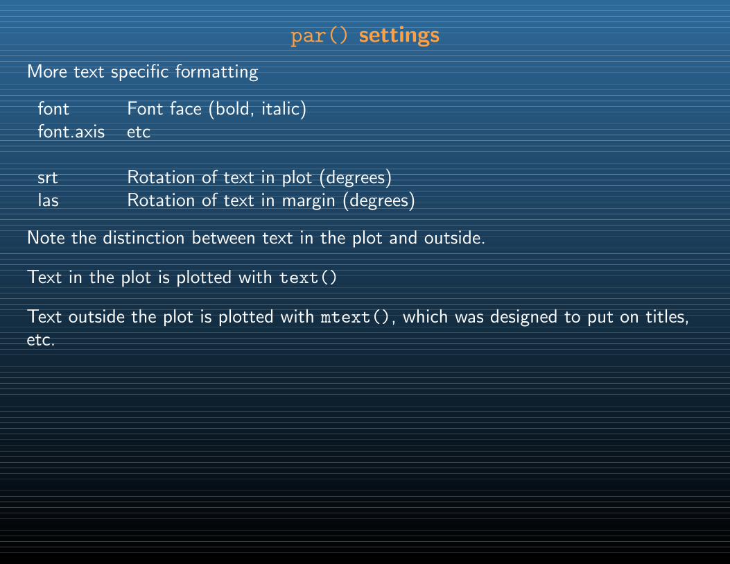
par() settings
More text specific formatting
font Font face (bold, italic)font.axis etc
srt Rotation of text in plot (degrees)las Rotation of text in margin (degrees)
Note the distinction between text in the plot and outside.
Text in the plot is plotted with text()
Text outside the plot is plotted with mtext(), which was designed to put on titles,etc.
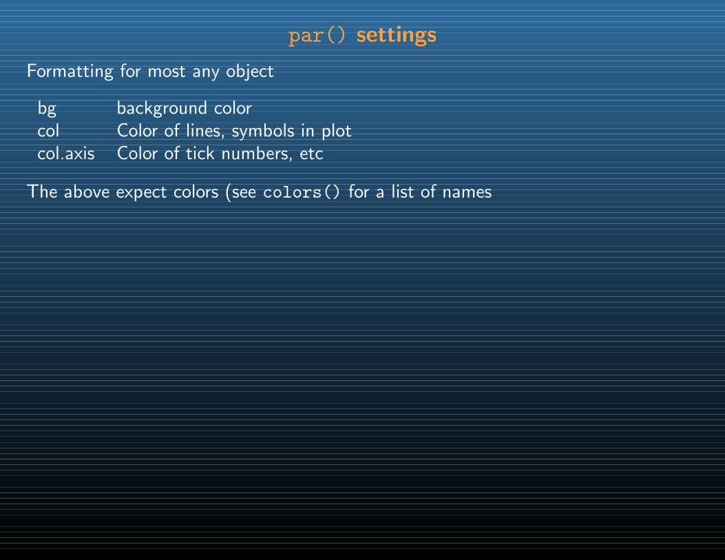
par() settings
Formatting for most any object
bg background colorcol Color of lines, symbols in plotcol.axis Color of tick numbers, etc
The above expect colors (see colors() for a list of names
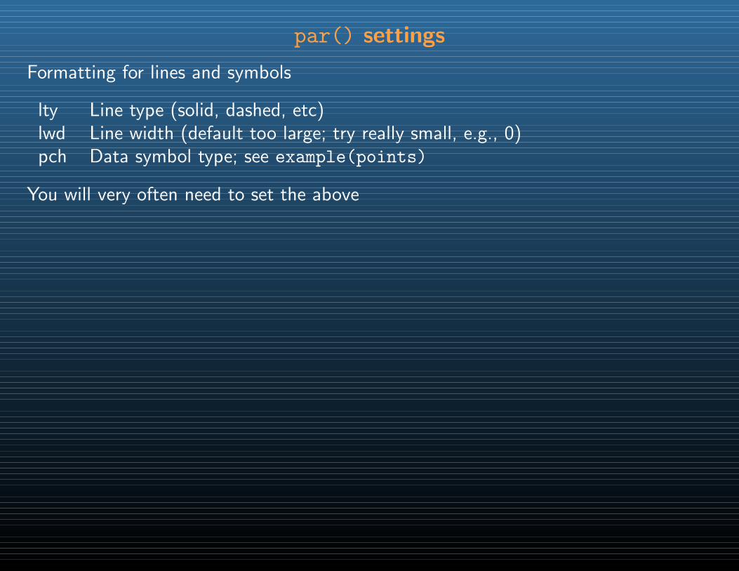
par() settings
Formatting for lines and symbols
lty Line type (solid, dashed, etc)lwd Line width (default too large; try really small, e.g., 0)pch Data symbol type; see example(points)
You will very often need to set the above
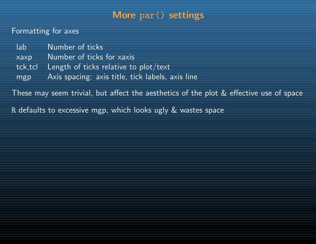
More par() settings
Formatting for axes
lab Number of ticksxaxp Number of ticks for xaxistck,tcl Length of ticks relative to plot/textmgp Axis spacing: axis title, tick labels, axis line
These may seem trivial, but affect the aesthetics of the plot & effective use of space
R defaults to excessive mgp, which looks ugly & wastes space
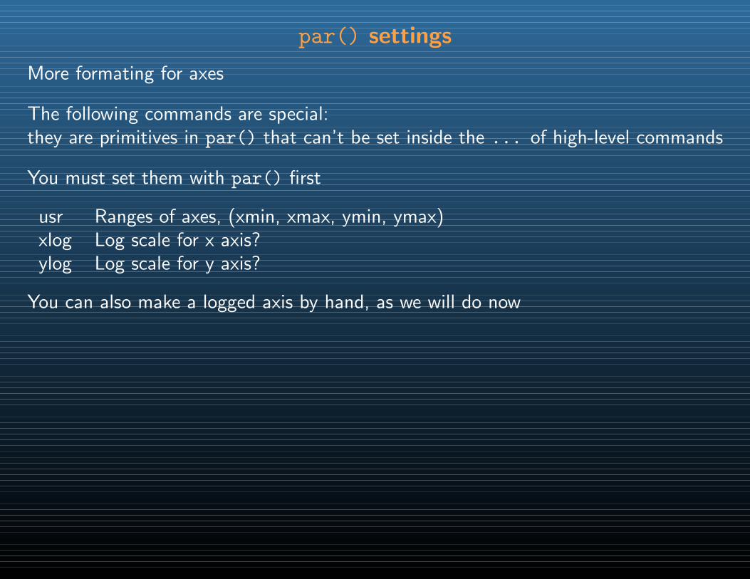
par() settings
More formating for axes
The following commands are special:they are primitives in par() that can’t be set inside the ... of high-level commands
You must set them with par() first
usr Ranges of axes, (xmin, xmax, ymin, ymax)xlog Log scale for x axis?ylog Log scale for y axis?
You can also make a logged axis by hand, as we will do now

Scatterplot: Occupational Prestige & Income
Classic data from sociology. Three variables
• Prestige of occupations, as rated by surveys
• Income of occupations (averaged across males)
• Type of occupation (blue collar, white collar, professional)
Data is in R. Look for Duncan.
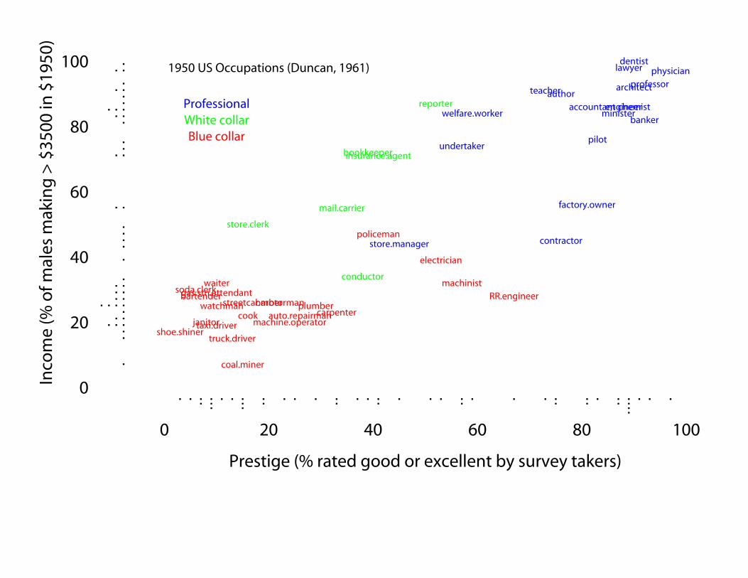
0 20 40 60 80 100
0
20
40
60
80
100
accountant
pilot
architectauthor
chemistminister
professor
dentist
reporter engineer
undertaker
lawyer physician
welfare.worker
teacher
conductor
contractor
factory.owner
store.manager
banker
bookkeeper
mail.carrier
insurance.agent
store.clerk
carpenter
electrician
RR.engineermachinist
auto.repairmanplumber
gas.stn.attendant
coal.miner
streetcar.motorman
taxi.drivertruck.driver
machine.operator
barberbartender
shoe.shiner
cook
soda.clerk
watchman
janitor
policeman
waiter
1950 US Occupations (Duncan, 1961)
ProfessionalWhite collarBlue collar
Prestige (% rated good or excellent by survey takers)
Inco
me
(% o
f mal
es m
akin
g >
$35
00 in
$19
50)
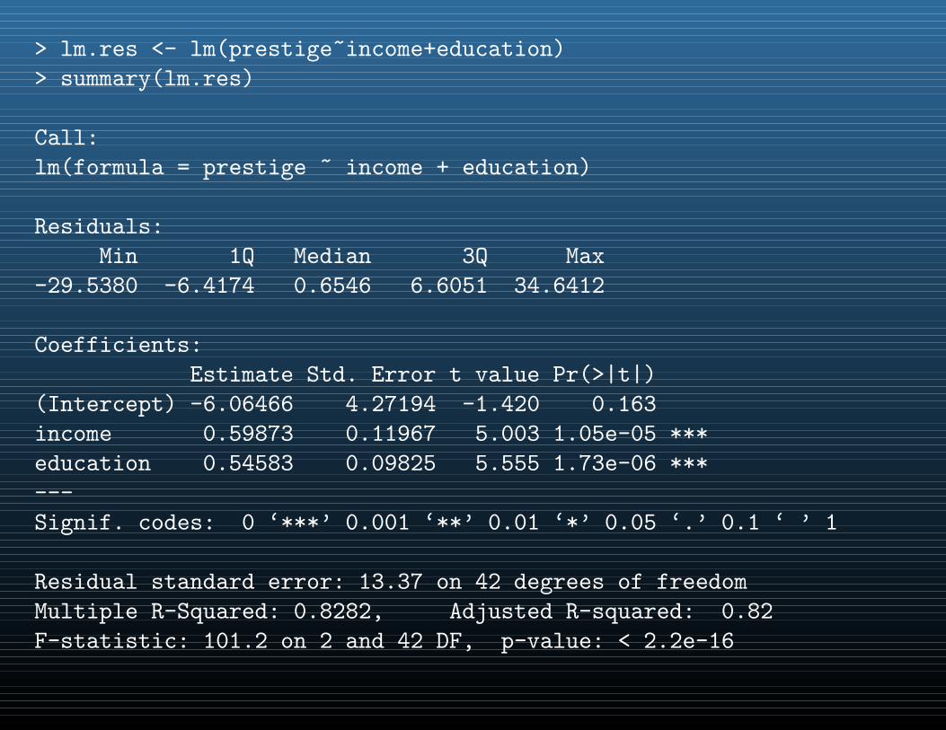
> lm.res <- lm(prestige~income+education)
> summary(lm.res)
Call:
lm(formula = prestige ~ income + education)
Residuals:
Min 1Q Median 3Q Max
-29.5380 -6.4174 0.6546 6.6051 34.6412
Coefficients:
Estimate Std. Error t value Pr(>|t|)
(Intercept) -6.06466 4.27194 -1.420 0.163
income 0.59873 0.11967 5.003 1.05e-05 ***
education 0.54583 0.09825 5.555 1.73e-06 ***
---
Signif. codes: 0 ‘***’ 0.001 ‘**’ 0.01 ‘*’ 0.05 ‘.’ 0.1 ‘ ’ 1
Residual standard error: 13.37 on 42 degrees of freedom
Multiple R-Squared: 0.8282, Adjusted R-squared: 0.82
F-statistic: 101.2 on 2 and 42 DF, p-value: < 2.2e-16
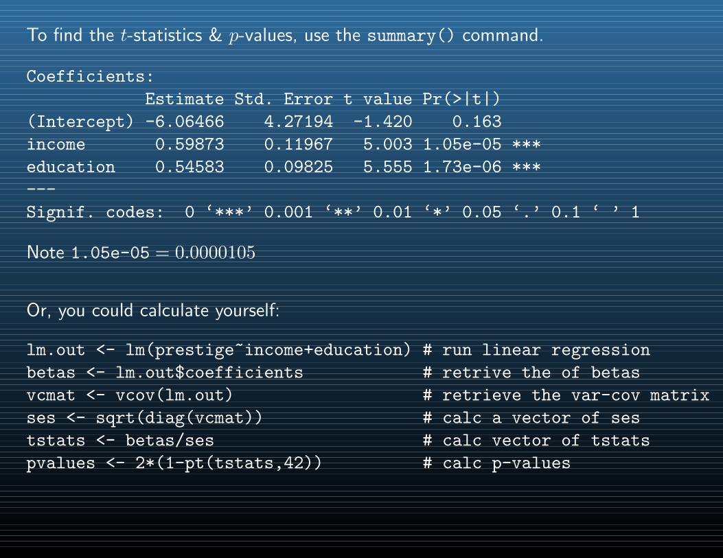
To find the t-statistics & p-values, use the summary() command.
Coefficients:
Estimate Std. Error t value Pr(>|t|)
(Intercept) -6.06466 4.27194 -1.420 0.163
income 0.59873 0.11967 5.003 1.05e-05 ***
education 0.54583 0.09825 5.555 1.73e-06 ***
---
Signif. codes: 0 ‘***’ 0.001 ‘**’ 0.01 ‘*’ 0.05 ‘.’ 0.1 ‘ ’ 1
Note 1.05e-05 = 0.0000105
Or, you could calculate yourself:
lm.out <- lm(prestige~income+education) # run linear regression
betas <- lm.out$coefficients # retrive the of betas
vcmat <- vcov(lm.out) # retrieve the var-cov matrix
ses <- sqrt(diag(vcmat)) # calc a vector of ses
tstats <- betas/ses # calc vector of tstats
pvalues <- 2*(1-pt(tstats,42)) # calc p-values
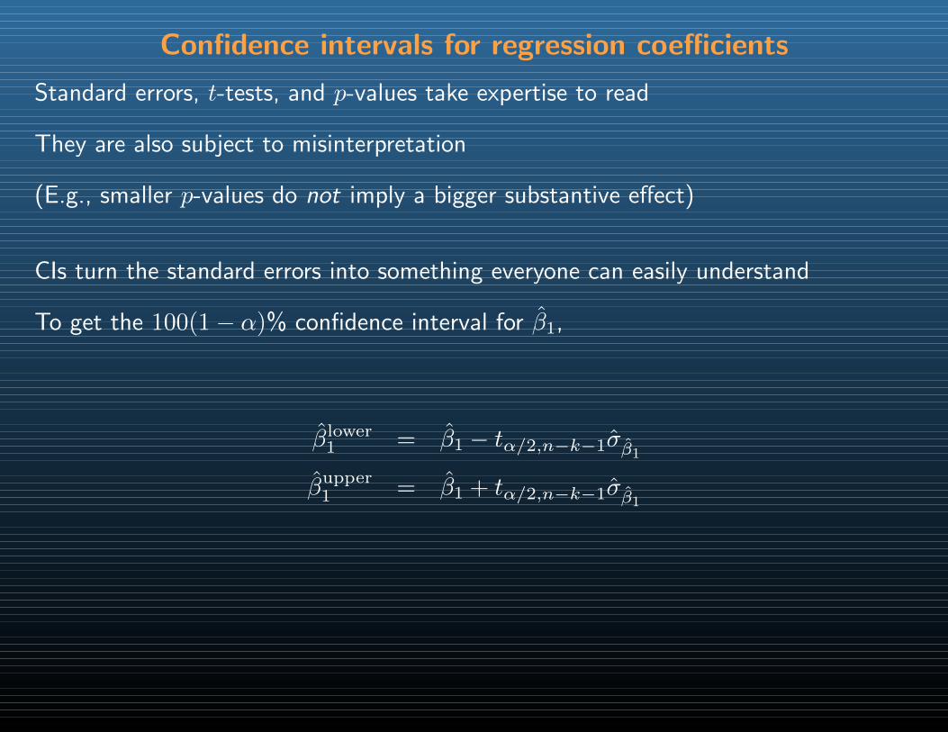
Confidence intervals for regression coefficients
Standard errors, t-tests, and p-values take expertise to read
They are also subject to misinterpretation
(E.g., smaller p-values do not imply a bigger substantive effect)
CIs turn the standard errors into something everyone can easily understand
To get the 100(1− α)% confidence interval for β1,
βlower1 = β1 − tα/2,n−k−1σβ1
βupper1 = β1 + tα/2,n−k−1σβ1
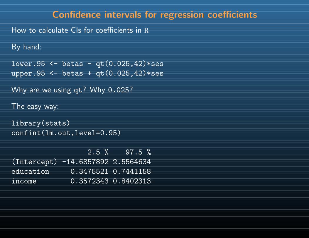
Confidence intervals for regression coefficients
How to calculate CIs for coefficients in R
By hand:
lower.95 <- betas - qt(0.025,42)*ses
upper.95 <- betas + qt(0.025,42)*ses
Why are we using qt? Why 0.025?
The easy way:
library(stats)
confint(lm.out,level=0.95)
2.5 % 97.5 %
(Intercept) -14.6857892 2.5564634
education 0.3475521 0.7441158
income 0.3572343 0.8402313
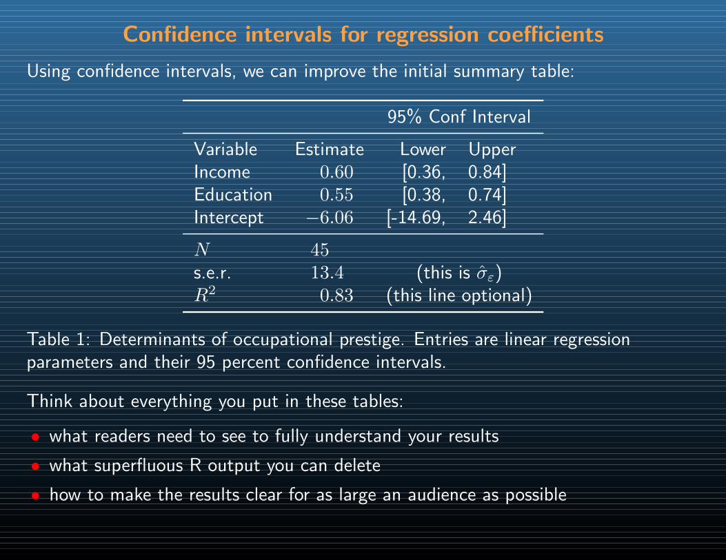
Confidence intervals for regression coefficients
Using confidence intervals, we can improve the initial summary table:
95% Conf Interval
Variable Estimate Lower UpperIncome 0.60 [0.36, 0.84]Education 0.55 [0.38, 0.74]Intercept −6.06 [-14.69, 2.46]
N 45s.e.r. 13.4 (this is σε)R2 0.83 (this line optional)
Table 1: Determinants of occupational prestige. Entries are linear regressionparameters and their 95 percent confidence intervals.
Think about everything you put in these tables:
• what readers need to see to fully understand your results
• what superfluous R output you can delete
• how to make the results clear for as large an audience as possible
Substantive & statistical significance
Don’t over interpret p-values
They only show statistical significance
Statistical and substantive significance can interact
A look at some hypothetical distributions of β1 helps frame the possibilities
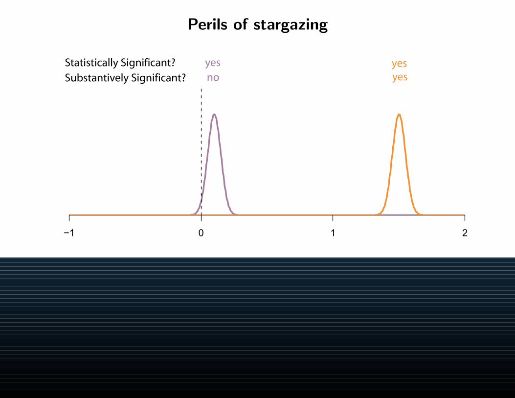
Perils of stargazing
−1 0 1 2
yesStatistically Significant? Substantively Significant? no
yesyes
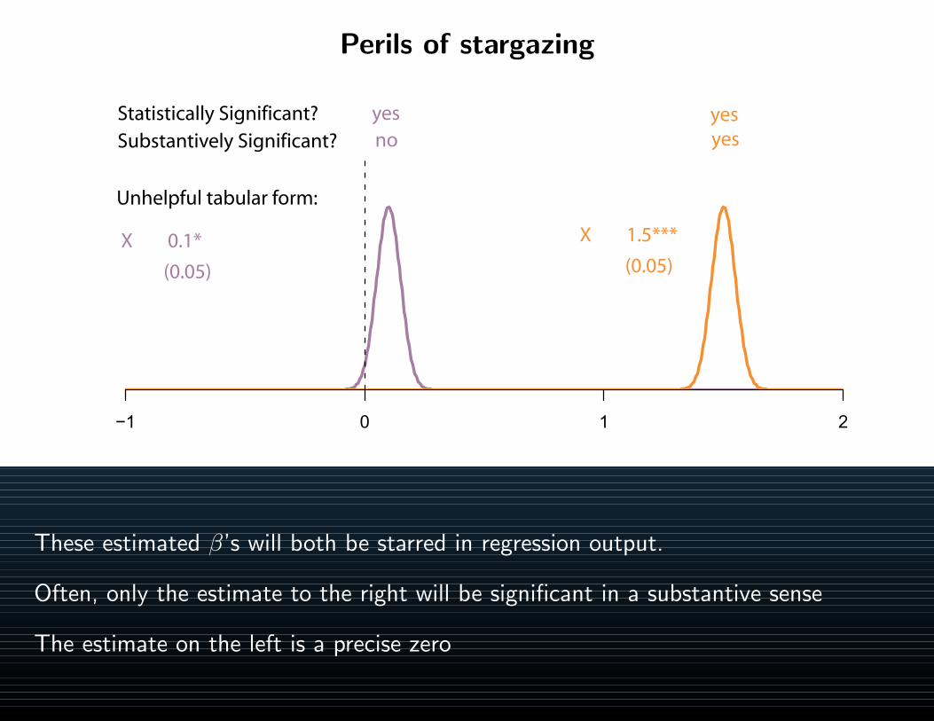
Perils of stargazing
−1 0 1 2
yesStatistically Significant? Substantively Significant? no
yesyes
Unhelpful tabular form:
X 0.1*
(0.05)
X 1.5***
(0.05)
These estimated β’s will both be starred in regression output.
Often, only the estimate to the right will be significant in a substantive sense
The estimate on the left is a precise zero

Perils of stargazing
−1 0 1 2
yes Statistically Significant? Substantively Significant? yes, but imprecise
yesyes, and precise
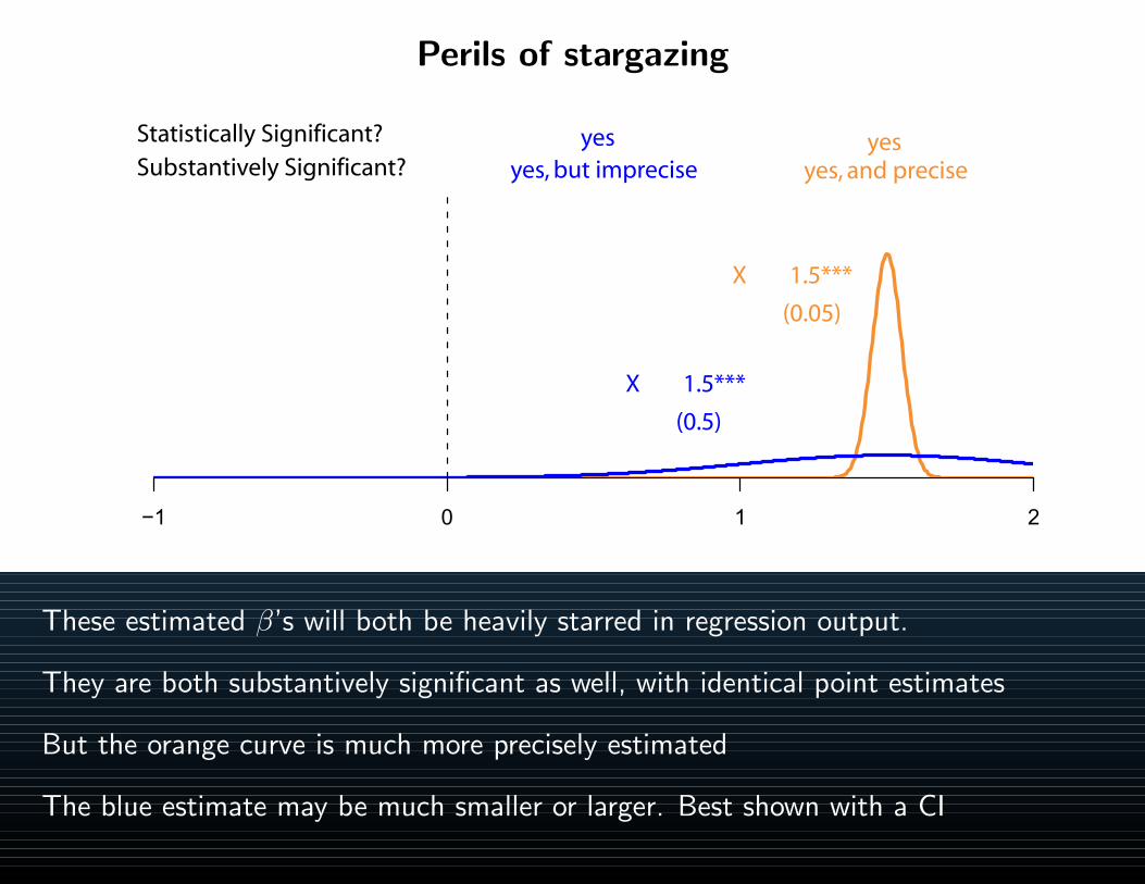
Perils of stargazing
−1 0 1 2
yes Statistically Significant? Substantively Significant? yes, but imprecise
yesyes, and precise
X 1.5***
(0.05)
X 1.5***
(0.5)
These estimated β’s will both be heavily starred in regression output.
They are both substantively significant as well, with identical point estimates
But the orange curve is much more precisely estimated
The blue estimate may be much smaller or larger. Best shown with a CI
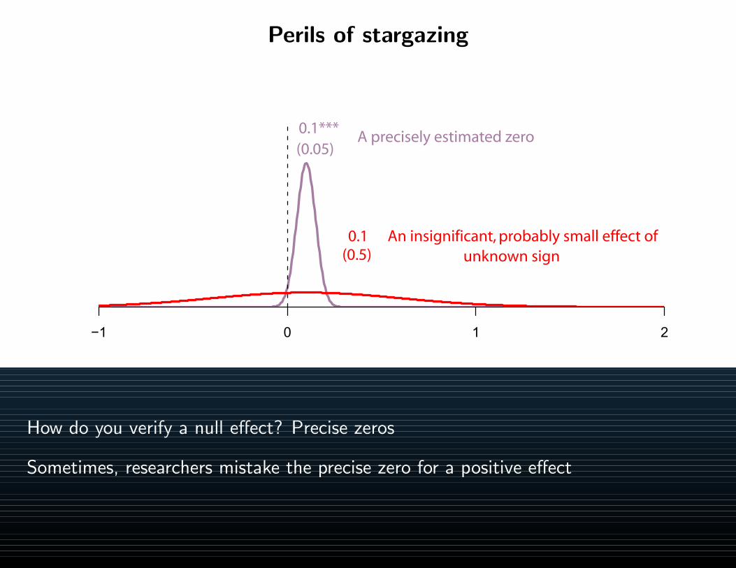
Perils of stargazing
−1 0 1 2
A precisely estimated zero
An insignificant, probably small effect of
0.1***
0.1unknown sign
(0.05)
(0.5)
How do you verify a null effect? Precise zeros
Sometimes, researchers mistake the precise zero for a positive effect
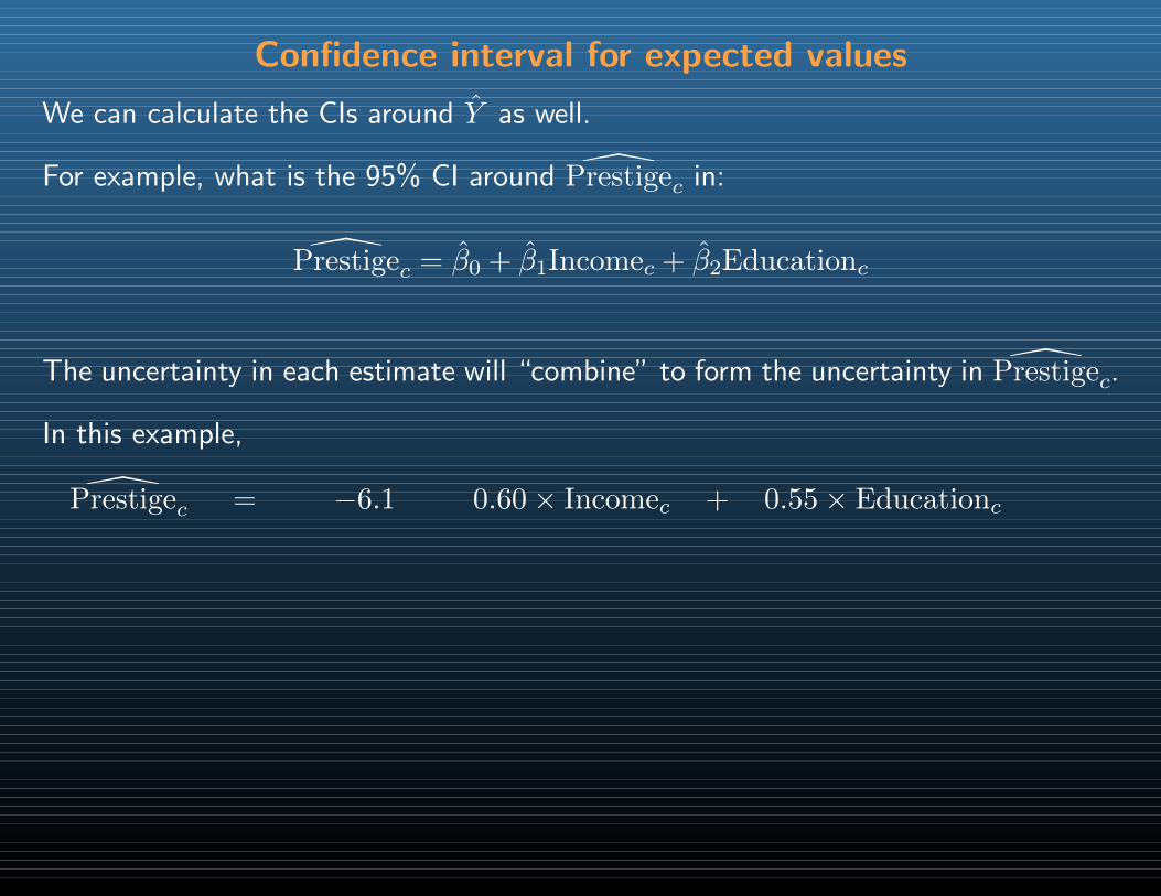
Confidence interval for expected values
We can calculate the CIs around Y as well.
For example, what is the 95% CI around Prestigec in:
Prestigec = β0 + β1Incomec + β2Educationc
The uncertainty in each estimate will “combine” to form the uncertainty in Prestigec.
In this example,
Prestigec = −6.1 0.60× Incomec + 0.55× Educationc

Confidence interval for expected values
We can calculate the CIs around Y as well.
For example, what is the 95% CI around Prestigec in:
Prestigec = β0 + β1Incomec + β2Educationc
The uncertainty in each estimate will “combine” to form the uncertainty in Prestigec.
In this example,
Prestigec = −6.1 0.60× Incomec + 0.55× Educationc[−14.7, 2.6] [0.36, 0.84] [0.35, 0.74]
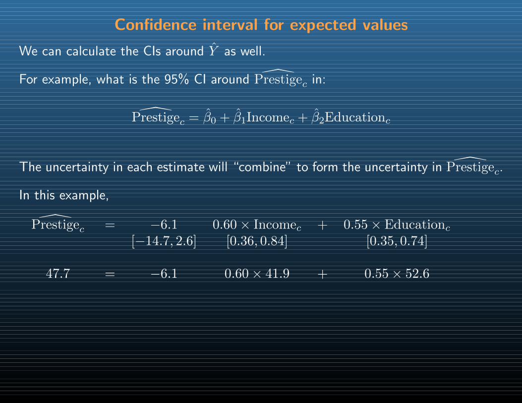
47.7 = −6.1 0.60× 41.9 + 0.55× 52.6
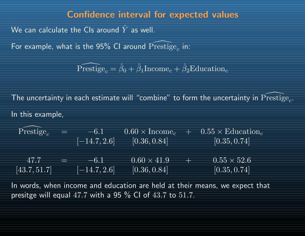
Confidence interval for expected values
We can calculate the CIs around Y as well.
For example, what is the 95% CI around Prestigec in:
Prestigec = β0 + β1Incomec + β2Educationc
The uncertainty in each estimate will “combine” to form the uncertainty in Prestigec.
In this example,
Prestigec = −6.1 0.60× Incomec + 0.55× Educationc[−14.7, 2.6] [0.36, 0.84] [0.35, 0.74]
47.7 = −6.1 0.60× 41.9 + 0.55× 52.6[43.7, 51.7] [−14.7, 2.6] [0.36, 0.84] [0.35, 0.74]
In words, when income and education are held at their means, we expect thatpresitge will equal 47.7 with a 95 % CI of 43.7 to 51.7.
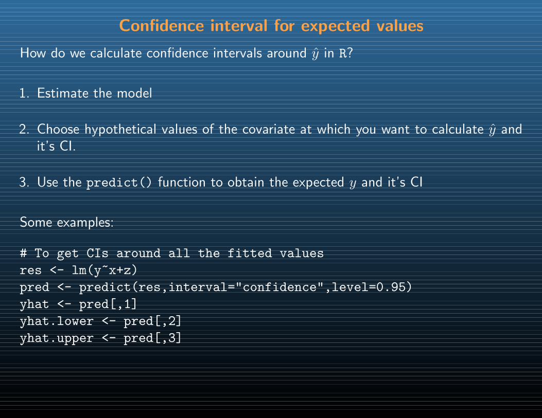
Confidence interval for expected values
How do we calculate confidence intervals around y in R?
1. Estimate the model
2. Choose hypothetical values of the covariate at which you want to calculate y andit’s CI.
3. Use the predict() function to obtain the expected y and it’s CI
Some examples:
# To get CIs around all the fitted values
res <- lm(y~x+z)
pred <- predict(res,interval="confidence",level=0.95)
yhat <- pred[,1]
yhat.lower <- pred[,2]
yhat.upper <- pred[,3]
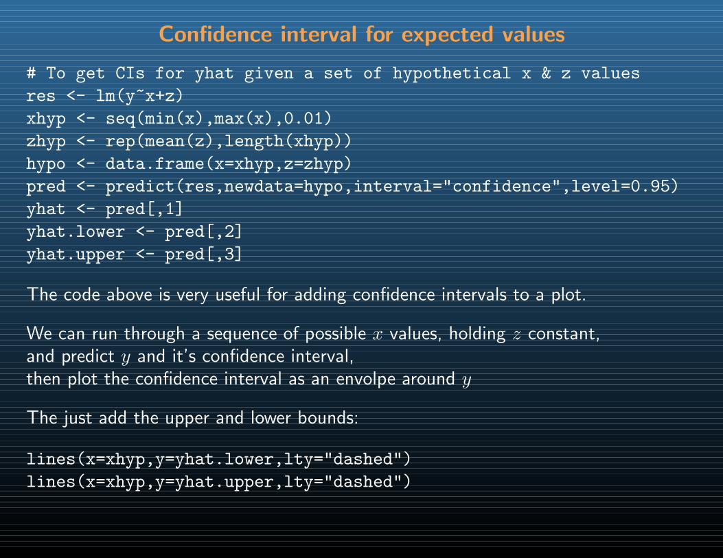
Confidence interval for expected values
# To get CIs for yhat given a set of hypothetical x & z values
res <- lm(y~x+z)
xhyp <- seq(min(x),max(x),0.01)
zhyp <- rep(mean(z),length(xhyp))
hypo <- data.frame(x=xhyp,z=zhyp)
pred <- predict(res,newdata=hypo,interval="confidence",level=0.95)
yhat <- pred[,1]
yhat.lower <- pred[,2]
yhat.upper <- pred[,3]
The code above is very useful for adding confidence intervals to a plot.
We can run through a sequence of possible x values, holding z constant,and predict y and it’s confidence interval,then plot the confidence interval as an envolpe around y
The just add the upper and lower bounds:
lines(x=xhyp,y=yhat.lower,lty="dashed")
lines(x=xhyp,y=yhat.upper,lty="dashed")
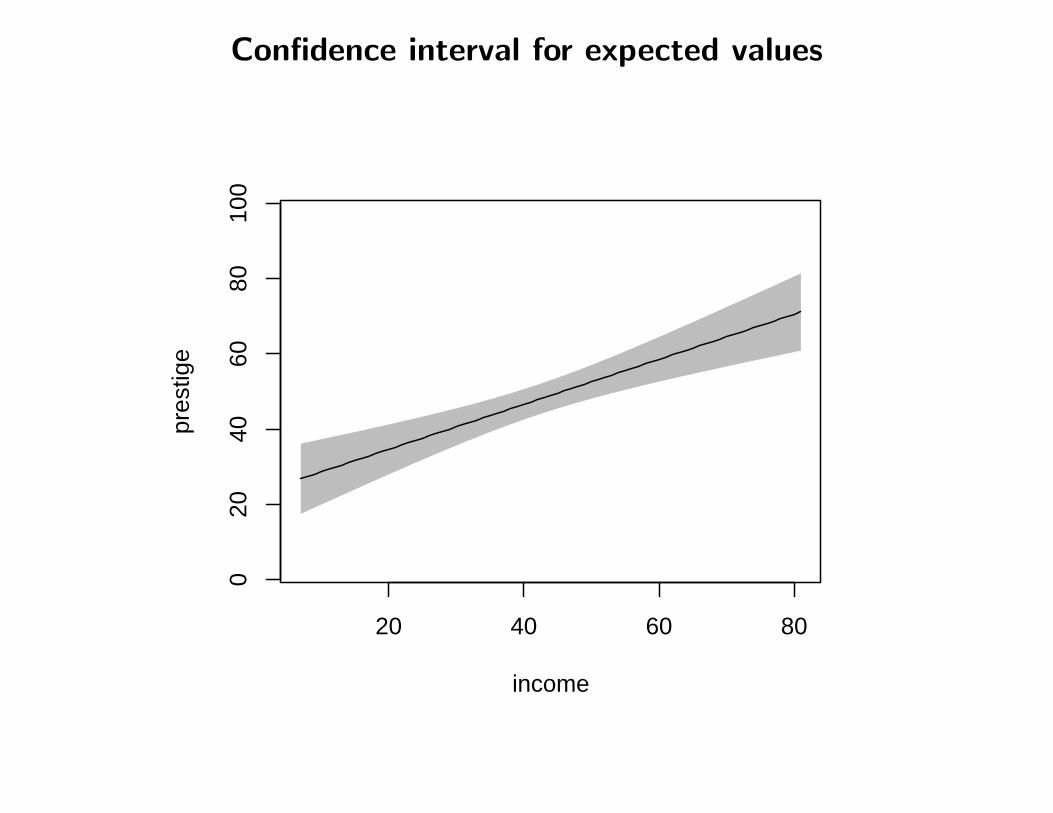
Confidence interval for expected values
20 40 60 80
020
4060
8010
0
income
pres
tige
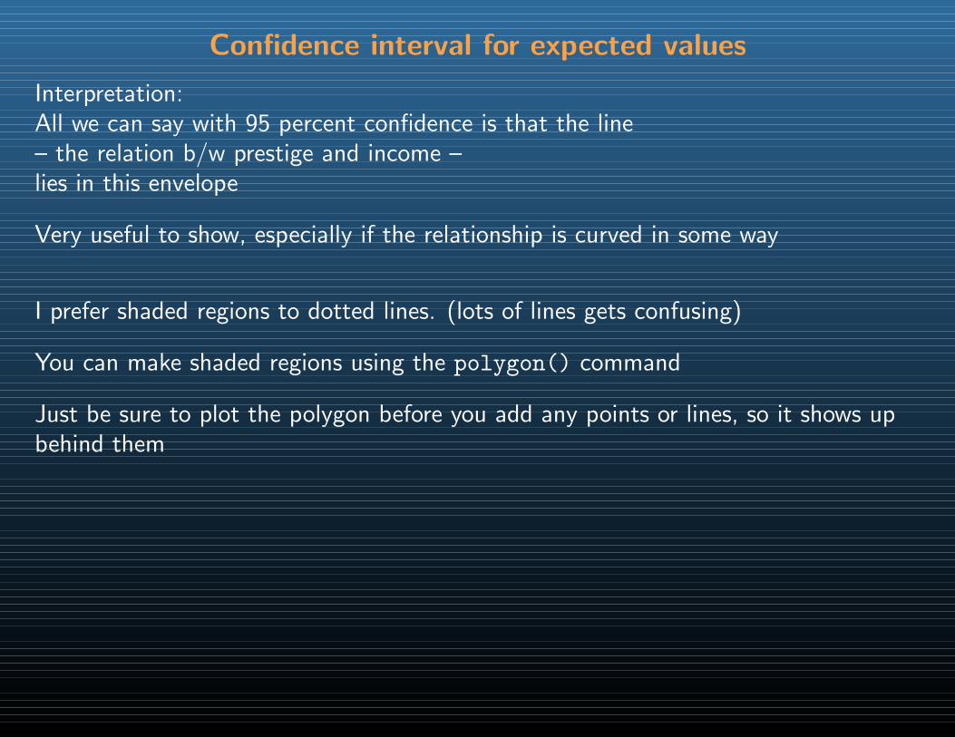
Confidence interval for expected values
Interpretation:All we can say with 95 percent confidence is that the line– the relation b/w prestige and income –lies in this envelope
Very useful to show, especially if the relationship is curved in some way
I prefer shaded regions to dotted lines. (lots of lines gets confusing)
You can make shaded regions using the polygon() command
Just be sure to plot the polygon before you add any points or lines, so it shows upbehind them
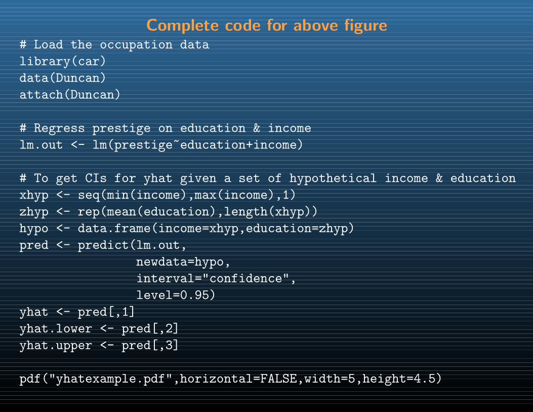
Complete code for above figure# Load the occupation data
library(car)
data(Duncan)
attach(Duncan)
# Regress prestige on education & income
lm.out <- lm(prestige~education+income)
# To get CIs for yhat given a set of hypothetical income & education
xhyp <- seq(min(income),max(income),1)
zhyp <- rep(mean(education),length(xhyp))
hypo <- data.frame(income=xhyp,education=zhyp)
pred <- predict(lm.out,
newdata=hypo,
interval="confidence",
level=0.95)
yhat <- pred[,1]
yhat.lower <- pred[,2]
yhat.upper <- pred[,3]
pdf("yhatexample.pdf",horizontal=FALSE,width=5,height=4.5)
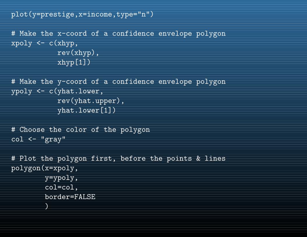
plot(y=prestige,x=income,type="n")
# Make the x-coord of a confidence envelope polygon
xpoly <- c(xhyp,
rev(xhyp),
xhyp[1])
# Make the y-coord of a confidence envelope polygon
ypoly <- c(yhat.lower,
rev(yhat.upper),
yhat.lower[1])
# Choose the color of the polygon
col <- "gray"
# Plot the polygon first, before the points & lines
polygon(x=xpoly,
y=ypoly,
col=col,
border=FALSE
)
# Plot the fitted line
lines(x=xhyp,y=yhat)
dev.off()