INTRODUCTION TO PROBABILITYThe goal of this lecture is to become familiar with the basics of probability theory and to understand relationships of probabilities

Objectives

After this lecture you should be able to: Describe uncertainty using probability terms

Determine how likely an event is to occur

Combine information regarding more than one event

Solve probability problems for use in decision making

Introduction

Probabilities are useful for answering questions What is the “chance” that sales will decrease if the

price of the product is increased? What is the “likelihood” that the new assembly method

will increase productivity? How “likely” is it that the project will be completed on

time? What are the “odds” that the new investment will be

profitable given that corn prices are low?

Analyzing Uncertainty

Random experiments A process or course of action that results in one of a

number of possible outcomes The sample space is the set of all possible

experimental outcomes Outcomes must be mutually exclusive and collectively

exhaustive Any one particular event is referred to as an outcome

from the experiment

Random Experiment - Tossing a Coin

The events are Heads & Tails These are the only two possibilities (collectively

exhaustive) The result must either be heads or tails and cannot be

both (mutually exclusive) An outcome would be Heads or Tails

Relative frequency, Theoretical, and Subjective Probabilities

Probability of an Event

© Purdue 2010

How likely is an Event?

Probability of an Event A number between 0 (never happens) and

1 (always happens) (often expressed as a percentage) The likelihood of occurrence of an event

Each random experiment has many probability numbersOne probability number for each event

Farm Income Ranges Examples

Assigning Probabilities

Two General Rules for Probabilities The probability assigned to each sample point must be

between 0 and 1(often expressed as a percentage) The sum of all of the experimental outcomes’

probabilities must be 1

Approaches to Assigning Probabilities

Relative frequency

Subjective

Theoretical

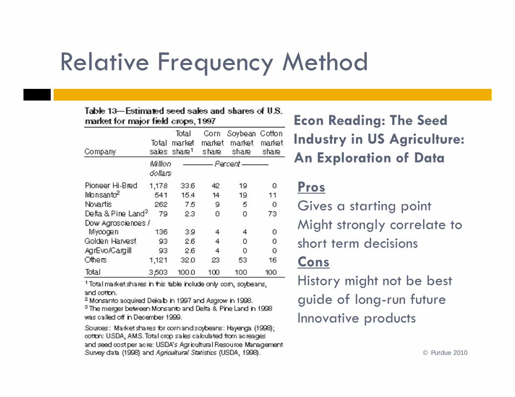
Relative Frequency Method

Expresses an outcome’s probability as the long-runrelative frequency of occurrence

This is also known as the empirical probability

Using the Law of Large Numbers Relative frequency is good “best guess” The larger the sample the better

Relative Frequency Method

© Purdue 2010

Econ Reading: The Seed Industry in US Agriculture: An Exploration of Data

Pros Gives a starting pointMight strongly correlate to short term decisionsConsHistory might not be best guide of long-run futureInnovative products

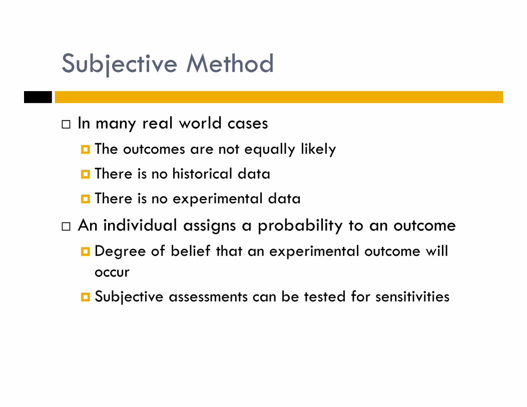
Subjective Method

In many real world cases The outcomes are not equally likely There is no historical data There is no experimental data

An individual assigns a probability to an outcome Degree of belief that an experimental outcome will

occur Subjective assessments can be tested for sensitivities

Subjective Method

What probabilities are associated with potential farm economy outcomes? Agricultural economy growth – 30% Agricultural economy stable – 50% Agricultural economy decline – 20%

Options need to be mutually exclusive and collectively exhaustive

© Purdue 2010

Theoretical Method

An experiment has “n” possible outcomes Each outcome is equally likely Probability of one outcome’s occurrence is 1/n

The coin flip example Coin landing heads is as equally likely as landing tails “n” = 2 (heads or tails) Probability of heads is ½ Probability of tails is also ½

Theoretical Method

Roll Expected2 2.78% (1/36)3 5.56% (2/36)4 8.33% (3/36)5 11.11% (4/36)6 13.89% (5/36)7 16.67% (6/36)8 13.89% (5/36)9 11.11% (4/36)

10 8.33% (3/36)11 5.56% (2/36)12 2.78% (1/36)

© Purdue 2010

Venn Diagrams and Conditional Probabilities

© Purdue 2010

Combining Events

Complement of the event A Happens whenever A does not happen

Union of events A and B Happens whenever either A or B or both events happen

Intersection of A and B Happens whenever both A and B happen

Conditional probability of A given B The updated probability of A, possibly changed to

reflect the fact that B has happened

Complement of an Event

The event “not A” happens whenever A does not Venn diagram: A (in circle), “not A” (shaded)

Probability(not A) = 1 – Prob(A) If Prob(Succeed) = 0.7, then Prob(Fail) = 1–0.7 = 0.3

Anot A(complement)

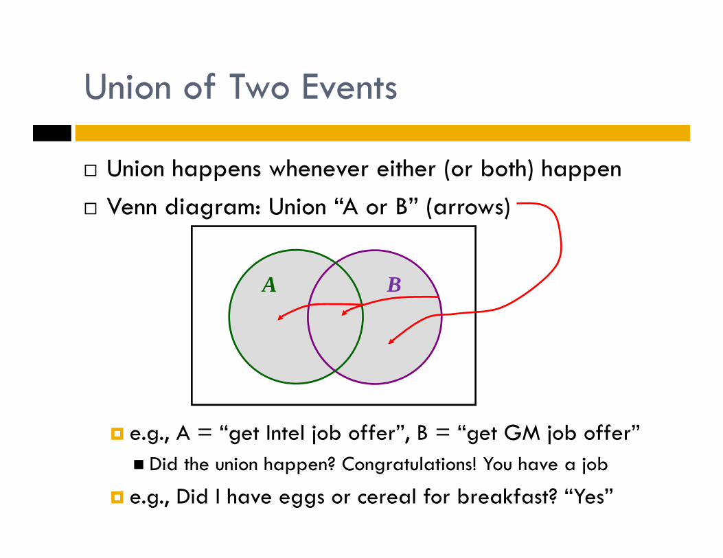
Union of Two Events

Union happens whenever either (or both) happen Venn diagram: Union “A or B” (arrows)

e.g., A = “get Intel job offer”, B = “get GM job offer” Did the union happen? Congratulations! You have a job

e.g., Did I have eggs or cereal for breakfast? “Yes”

A B

Intersection of Two Events

Intersection happens whenever both events happen Venn diagram: Intersection “A and B” (arrow)

e.g., A = “sign contract”, B = “get financing” Did the intersection happen? Project has been launched! e.g., Did I have eggs and cereal for breakfast? “No”

A B

Twitter is the intersection

© Purdue 2010

Relationship Between and and or

Prob(A or B) = Prob(A)+Prob(B)–Prob(A and B)

= + –

Prob(A and B) = Prob(A)+Prob(B)–Prob(A or B)

Farm location and type

Prob(Fruitful Rim) = 0.119 Prob(Residential/lifestyle) = 0.451 Prob(Fruitful Rim and Residential/Lifestyle) = 0.048

Then we must have Prob(Fruitful Rim or Residential/Lifestyle) = 0.119+0.451–

0.048 = 0.522

The Conditional Probability

In many probability situations, being able to determine the probability of one event when another event is known to have occurred is important

Suppose that we have an event A with probability P(A) and that we obtain new information or learn that another event B has occurred

If A is related to B we want to take advantage of this information

The Conditional Probability

The new probability of event A is written P(A|B) which is read as the probability of A given the condition that B has occurred

The general definition is:

Event A • Event B

The light shaded region denotes that B has occurred

Probability of A and B

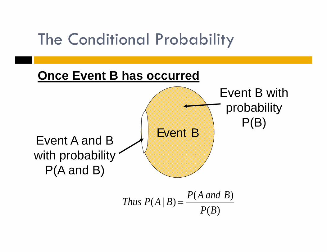
The Conditional Probability

Event B

Once Event B has occurred

Event A and B with probability

P(A and B)

Event B with probability

P(B)

)()()|(

BPBandAPBAPThus

Seed Adoption

Illinois Farmers Prob(grows corn) = 0.70, Prob(early adopter) =

0.135, Prob(grows corn and early adopter) = 0.07

Conditional probability of early adopter given that they grow corn P(early adopter | grows corn) = Prob (early adopter

and grows corn)/Prob (grows corn) = 0.07/0.70 = .10 10% of corn farmers are early adopters

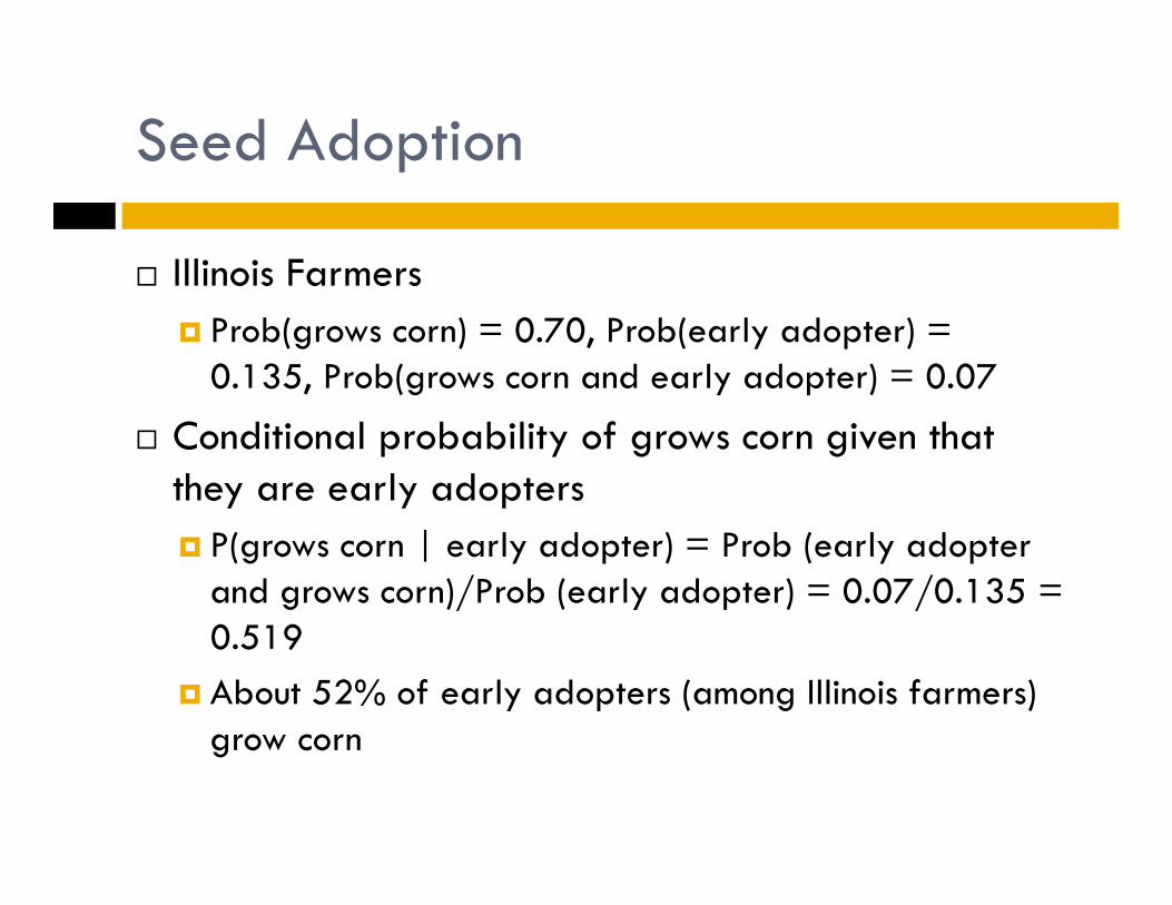
Seed Adoption

Illinois Farmers Prob(grows corn) = 0.70, Prob(early adopter) =

0.135, Prob(grows corn and early adopter) = 0.07

Conditional probability of grows corn given that they are early adopters P(grows corn | early adopter) = Prob (early adopter

and grows corn)/Prob (early adopter) = 0.07/0.135 = 0.519

About 52% of early adopters (among Illinois farmers) grow corn

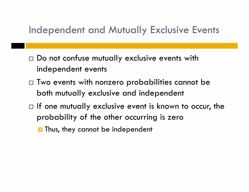
Independent and Mutually Exclusive Events

Do not confuse mutually exclusive events with independent events

Two events with nonzero probabilities cannot be both mutually exclusive and independent

If one mutually exclusive event is known to occur, the probability of the other occurring is zero Thus, they cannot be independent

Method for Solving Probability Problems

Given probabilities for some events (perhaps union, intersection, or conditional) Find probabilities for other events

Use a probability tree

Probability Tree

Record the basic information on the tree Usually three probability numbers are given The tree helps guide your calculations

Each column of circled probabilities adds up to 1 Circled probability times conditional probability gives

next probability For each group of branches Conditional probabilities add up to 1 Circled probabilities at end add up to probability at start

© Purdue

Probability Tree

Shows probabilities and conditional probabilities

P(A and B)

P(A and “not B”)

P(“not A” and B)

P(“not A” and “not B”)

P(A)

P(not A)

Event B

Event A

Venn Diagram

Venn diagram probabilities correspond to right-hand endpoints of probability tree

Corn grower0.63

Early adopter0.0650.07

0.235

P(“corn grower” and “early adopter”)P(“corn grower” and “not early adopter”) P(“not corn grower” and early adopter)

P(“not fertilizer” and “not chemicals”)

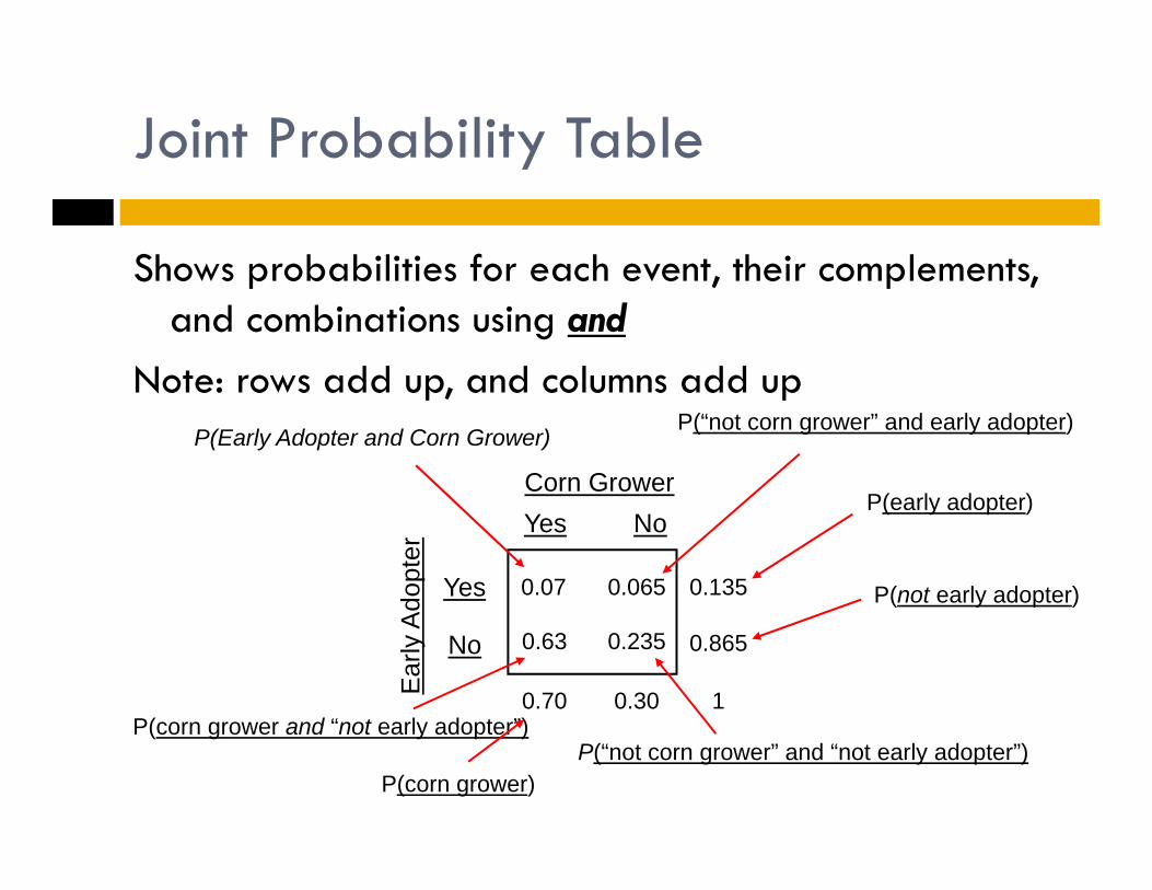
Joint Probability Table

Shows probabilities for each event, their complements, and combinations using and

Note: rows add up, and columns add up

Corn GrowerYes No

Ear

ly A

dopt

er

Yes

No

0.30 1

0.07

P(Early Adopter and Corn Grower)

0.065

P(“not corn grower” and early adopter)

0.235

P(“not corn grower” and “not early adopter”)

0.63

P(corn grower and “not early adopter”)

0.135

P(early adopter)

0.865

P(not early adopter)

0.70

P(corn grower)

Summary

You should now have a good understanding of Experiments Assigning Probabilities Probability Rules

Review these concepts as often as necessary to become familiar with them

Assignment 2 will give you another opportunity to review and apply this material