stat 225: introduction to probability models course ...mrlawlor/student_notes.pdf · stat 225:...

STAT 225: Introduction to Probability Models

Course Lecture Notes

1 Introduction to Probability

1.1 Set Theory

The material in this handout is intended to cover general set theory topics. Information includes(but is not limited to) introductory probabilities, outcome spaces, sample spaces, laws of probabil-ity, and Venn Diagrams. This covers section 1.2 and all of chapter 2 from A Course in Probabilityby Neil Weiss.

An element is a single item (outcome), typically denoted by ω.

A set is a collection of elements.

A subset is a set itself, in which every element is contained in a larger set. Suppose the set Ais contained in the set B. This is denoted by A ⊂ B or A ⊆ B depending on whether or not Bhas elements which are not in A. If B contains elements that are not in A, then A is called aproper subset of B.

A Population is the collection of all individuals or items under consideration. An individual couldrefer to a person, a playing card, or whatever object we are interested in. A population is used inreference to sampling. However, when we talk about experiments, we use the phrase sample space.

Sample space is the set of all possible outcomes for a random experiment and is denoted by Ω.Random Experiment is an action whose outcome cannot be predicted with certainty beforehand.

Example 1.1 Suppose we are interested in whether the price of the S & P 500 decreases, stays the same,or increases. If we were to examine the S & P 500 over one day, then Ω = decreases, staysthe same, increases. What would Ω be if we looked at 2 days?

The opposite of Ω is the empty (null) set. It is the set with 0 elements in it and is written as ∅.(Please note how this looks. Do not write your 0s like this or you will lose points as they have2 very different meanings.) Ω and ∅ are complements. A complement is a set that contains allof the elements in the sample space that are not in the original set. We denote a complementwith a superscript c (or C). For example, the complement of A would be denoted as Ac or AC .Sometimes the symbol \ is useful when writing complements. The symbol \ means ”except” or”everything but”. Suppose we look at the outcome of 2 rolls of a die. Let A be the event thatboth rolls are a 5. Then AC = Ω \ 5, 5. We use the symbol ∈ to denote ”belongs to”. Here isthe symbol for ”does not belong to”: 6∈.

1 of 62

Here are some important sets that pertain to numbers: the real numbers R , the integers Z, therational numbers Q, the natural (whole) numbers N, and the positive integers Z+. What sets arecontained in (or are subsets of) the other sets?

Example 1.2 Let us examine what happens in the flip of 3 fair coins. Fair means that the coin has thesame probability of landing as a head as it does as landing as a tail. First, define Ω. Let Abe the event of exactly 2 tails. Let B be the event that the first 2 tosses are tails. Let Cbe the event that all 3 tosses are tails. Write out the possible outcomes for each of these 3events. We will revisit these events later on.

Example 1.3 Let Ω, the universal set, be all 26 lower-case letters. Define the sets V , N , E, and G (all ofwhich are subsets of Ω) as follows:

• V = vowels (here, assume “y” is a vowel) =

• N = letters next to a vowel (in the natural sequence “a” - “z”) =

• E = every other letter, starting with “b” =

• G = letters “a” - “g” =

List the letters in each of the following sets:

• V , N , E, and G individually (see answers above)

• NC =

• GC =

Example 1.4 Start with a standard deck of 52 cards and remove all the hearts and all the spades, leaving13 red and 13 black cards. List the cards in each of the following sets:

• N = not a face card

• R = neither red nor an ace

• E = either black, even, or a Jack

Example 1.5 Suppose a fair six-sided die is rolled twice. Determine the number of possible outcomes

• for this experiment.

• in which the sum of the two rolls is 5.

• in which the two rolls are the same.

• in which the sum of the two rolls is an even number.

Random Experiment is an action whose outcome cannot be predicted with certainty beforehand.This does not mean that we know nothing about what can happen. An example of a randomexperiment could be one roll of a die (or multiple rolls), a hand in Texas Hold ’em, or a gradein a course. Ω represents all possible outcomes from the random experiment or the model underconsideration.

An event is defined to be any subset of the sample space. It can be one or more outcomes.Typically, when we refer to an event that is a single outcome, it is called a simple event, and

2 of 62

subsequently, a simple probability. For an example, you could think of an event as not losingmoney on the S & P 500 on a given day. This event has 2 outcomes based on Example 1.1 whereΩ = decreases, stays the same, increases.

Example 1.6 Refer to Example 1.1. Suppose you looked at 2 consecutive days for this index. Let A bethe event that you made money on the first day. Let B be the event that you had at leastone day where you made money. How many outcomes does each event represent?

1.2 Probability

The Frequentist Interpretation of Probability states that the probability of an event is thelong-run proportion of times that the event occurs in independent repetitions of the randomexperiment. This is referred to as an empirical probability and can be written as

P (E) =N(E)

n

where n represents the sample size. (For definitions of P(E) and N(E) see the symbols reference.)Long-run means that n is large. There are differing viewpoints on large (typical examples are >100, > 1,000, > 1,000,000, etc.) We will not use this exact formula for now, but it is essential tothe Central Limit Theorem (CLT), which will be covered in MGMT 305. However, the conceptis applicable for our purposes. Regardless of the sample size, if we are in an EQUALLY LIKELYFRAMEWORK, then

P (E) =N(E)

N(Ω).

What is meant by an equally likely framework? Well, let us create a scenario that has sucha property. Suppose we roll a fair, 6-sided die. Because the die is fair, each side of the diehas the same probability of occurring as any other side of the die. Therefore, any individualoutcome of the sample space is equally likely as any other outcome in the sample space. Of-ten, the equal-likelihood model is referred to as classical probability. So, in an equally likelyframework, the probability of any event is the number of ways the event occurs divided by thenumber of total events possible. Find the probabilities associated with parts 2-4 of Example 1.5.

1.3 Probability Rules

Regardless of whether sample outcomes have the same probabilities, there are rules that proba-bilities must satisfy.

• Any probability must be between 0 and 1 inclusive.

• Additionally, the sum of the probabilities for all the experimental outcomes must equal 1.

• Suppose the event E is composed of several outcomes. Then the probability of E is just thesum of the probabilities of those outcomes.

3 of 62

If a probability model satisfies the first two rules, it is said to be legitimate. Refer to event Bin Example 1.2 for as an example of the third rule above.

What are the probabilities of Ω, ∅?

If A ⊂ B, what (if anything) can you say about their probabilities?

Example 1.7 (ASW Chapter 4.1, Problem 6) An experiment with three outcomes has been repeated 50times, and it was learned that E1 occurred 20 times, E2 occurred 13 times, and E3 occurred17 times. Assign probabilities to the outcomes. What method did you use?

Example 1.8 Start with a standard deck of 52 cards and remove all the hearts and all the spades, leaving13 red and 13 black cards. Suppose a card is randomly drawn from the remaining cards.What are the probabilities of the following events?

• N = not a face card

• R = neither red nor an ace

• E = either black, even, or a Jack

Example 1.9 (ASW Chapter 4.1, Problem 7) A decision maker subjectively assigned the following prob-abilities to the four outcomes of an experiment: P (E1) = .10, P (E2) = .15, P (E3) = .40,and P (E4) = .20. Are these probability assignments legitimate? Explain.

1.4 Probability with Several Events

The intersection of the events A and B is written as A ∩ B. For an outcome to belong to theintersection, that outcome has to be in both A and B. If we were talking about the intersectionof 3 or more events, the outcome would need to be in all of them. The intersection is what is incommon.

The union of the events A and B is written as A ∪ B and it means whatever is in at least one ofA or B. Please note that we do not double count. If an outcome was in both A and B, then it isin their union, but it is not in there twice.

Example 1.10 Refer to Example 1.2, where we flipped 3 fair coins: What are A ∩ B, A ∪ C, and A ∩ B∪ C?

Two other useful terms are mutually exclusive and exhaustive. Mutually exclusive refers to two(or more) events that cannot both occur when the random experiment is formed. Can you think ofan event that is mutually exclusive with event C from Example 1.2? Note that the term disjoint isthe same as mutually exclusive except that it refers to sets and not events. One can symbolicallydenote mutually exclusive events by the following equation: A ∩ B = ∅.

4 of 62

Exhaustive refers to event(s) that comprise the sample space. In other words, events that areexhaustive have a union that equals the sample space; if A and B are exhaustive, then A ∪ B = Ω.

What would you call events that are both mutually exclusive and exhaustive? The answer is apartition. What is the simplest partition?

Venn Diagrams are useful tools for examining the relationships between events. Tree diagramsare also helpful (more on this when we come to conditional probability, general multiplication rule,etc.) Draw generic diagrams for events that are: mutually exclusive, exhaustive, complements,subsets, and have an intersection but are not subsets.

The complement rule is a way to calculate a probability based on the probability of its comple-ment. It is

P (A) = 1− P (AC).

This law is extremely useful. It is often handy in situations where the desired event has manyoutcomes, but its complement has only a few.

Example 1.11 Suppose we rolled a fair, six-sided die 10 times. Let T be the event that we roll at least 1three. If one were to calculate T you would need to find the probability of 1 three, 2 threes,... , and 10 threes and add them all up. However, you can use the complement rule. Whatis P(T)?

The general addition rule is a way of finding the probability of a union of 2 events.

P (A ∪B) = P (A) + P (B)− P (A ∩B).

What does this become if A and B are mutually exclusive? Can you provide a mathematical proofof this?

The inclusion-exclusion principle is a way to extend the general addition rule to 3 or more events.Here we will limit it to 3 events.

P (A ∪B ∪ C) = P (A) + P (B) + P (C)− P (A ∩B)− P (A ∩ C)− P (B ∩ C) + P (A ∩B ∩ C).

The law of partitions is a way to calculate the probability of an event. Let A1, A2, ..., Ak form apartition of Ω. Then, for all events B,

P (B) =k∑i=1

P (Ai ∩B).

Then, there are DeMorgan’s Laws. Let A and B be subsets of Ω. Then

• (A ∪B)C = AC ∩BC .

5 of 62

• (A ∩B)C = AC ∪BC .

Example 1.12 Refer to Example 1.3. Solve for the following quantities:

• P (consonant) =

• P (GC) =

• P (E) and P (EC)

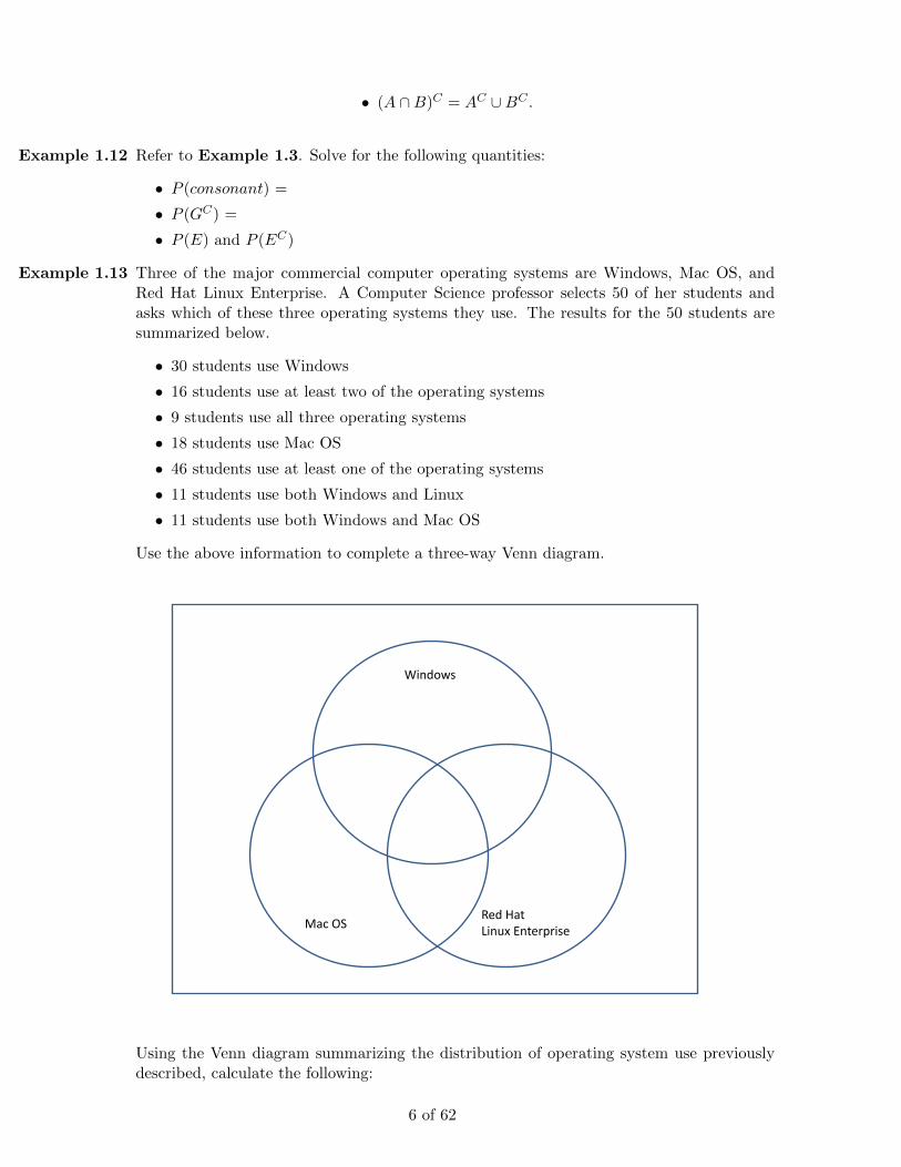
Example 1.13 Three of the major commercial computer operating systems are Windows, Mac OS, andRed Hat Linux Enterprise. A Computer Science professor selects 50 of her students andasks which of these three operating systems they use. The results for the 50 students aresummarized below.

• 30 students use Windows

• 16 students use at least two of the operating systems

• 9 students use all three operating systems

• 18 students use Mac OS

• 46 students use at least one of the operating systems

• 11 students use both Windows and Linux

• 11 students use both Windows and Mac OS

Use the above information to complete a three-way Venn diagram.

Windows

Mac OS Red Hat Linux Enterprise

Using the Venn diagram summarizing the distribution of operating system use previouslydescribed, calculate the following:

6 of 62

• Let Windows = W , Mac OS = M , and Red Hat Linux Enterprise = L

• N(WC ∩MC)

• P (WC ∪MC) =

• N(W ∪M ∪ L) =

Example 1.14 In a certain population, 10 % of the population are rich, 5 % are famous, and 3 % are both.

• Draw a Venn Diagram for the situation described above and label all probabilities.

• What is the probability a randomly chosen person is not rich?

• What is the probability a randomly chosen person is rich but not famous?

• What is the probability a randomly chosen person is either rich or famous?

• What is the probability a randomly chosen person is either rich or famous but notboth?

• What is the probability a randomly chosen person has neither wealth nor fame?

Example 1.15 Drew is a risk taker. On any given weekend, Drew takes risks with or without monetarycompensation. He gets paid 20 % of the time he takes risks. The risks involved are to eitherdrink something weird (like garlic butter) or do something silly (like shave his head into amohawk). Drew gets paid and drinks something weird 16 % of the time. Drew does not getpaid and drinks something weird 72 % of the time. What is the probability Drew drinkssomething weird? What is the probability he does something silly?

Here are a few of the other laws. Each pair of equations refers to the distributive, commutative,and associative laws respectively. For all of these, let A, B, and C be subsets of Ω.

A ∩ (B ∪ C) = (A ∩B) ∪ (A ∩ C)

A ∪ (B ∩ C) = (A ∪B) ∩ (A ∪ C).

A ∩B = B ∩A

A ∪B = B ∪A

A ∩ (B ∩ C) = (A ∩B) ∩ C.

A ∪ (B ∪ C) = (A ∪B) ∪ C.

Please be aware that the formulas just written can be extended to more than 3 events (even aninfinite number of events).

1.5 Counting Rules

The Basic Counting Rule, or BCR is used for scenarios that have multiple choices or actions to bedetermined. Suppose that r actions (choices) need to be performed (in a definite order). Furthersuppose that there are m1 possibilities for the 1st action, m2 possibilities for the 2nd action, etc.Then there are m1 ∗m2 ∗ ... ∗mr possibilities altogether for the r actions.

A factorial is the product of the 1st so many positive integers. Suppose we were looking at ageneric (positive) integer k. Then k factorial, denoted k!, is equivalent to k*(k-1)*(k-2)*...*1. For

7 of 62

a specific example, 4! is 4*3*2*1 = 24.

A permutation of r objects from a collection of n objects is any ORDERED arrangement of rdistinct objects from the n objects. This is written as either (n)r or nPr. Mathematically it isdefined to be n!

(n−r)! .

The special permutation rule states that anything permute itself is equivalent to itself factorial.As an example, (n)n = n! or (6)6 = 6!.

A combination of r objects from a collection of n objects is any UNORDERED arrangment of rdistinct objects from the n total objects. The difference between a combination and a permutationis that order of the objects is not important for a combination. A combination, say n choose r(as described above) is written as either nCr or

(nr

). Mathematically,

(nr

)is equal to (n)r

r! which is

also equal to n!(n−r)!∗r! .

An ordered partition of m objects into k distinct groups of sizes m1,m2, ...,mk is any divisionof the m objects into a combination of m1 objects constituting the first group, m2 objects com-prising the second group, etc. The number of such partitions that can be made is denoted by(

mm1,m2,...,mk

). Mathematically, this is equal to m!

m1!∗m2!∗...∗mk! . The symbol used in evaluatingan ordered partition is called a multinomial coefficient. You may hear your instructor use bothordered partition and multinomial coefficient.

Example 1.16 3 people get into an elevator and choose to get off at one of the 10 remaining floors. Findthe following probabilities:

• P(they all get off on different floors)

• P(they all get off on the 5th floor)

• P(they all get off on the same floor)

• P(exactly one of them gets off on the 5th floor)

• P(at LEAST one of them gets off on the 5th floor)

Example 1.17 Suppose we have the fictional word DALDERFARG.

• How many ways are there to arrange all of the letters?

• What is the probability that the 1st letter is the same as the 2nd letter?

• What is the probability that an arrangement of all of the letters has the 2 Ds next toeach other?

8 of 62

• What is the probability that an arrangement of all of the letters has the 2 Ds next toeach other and it has the 2 Rs grouped together (not necessarily the Ds and Rs nextto each other)?

• What is the probability that an arrangement of all the letters has the 2 Ds before the F?

Example 1.18 Illinois license plates consist of 4 digits followed by 2 letters. Whereas, in Ohio, licenseplates start with 3 letters and end with 4 digits. Assume all letters are capitals (withoutloss of generality, or wlog).

• For each state, how many possible license plates are there?

• How many possible license plates are there for each state if no digit or letter is allowedto repeat?

• How many possible license plates are there if they must have at least 1 vowel?

• How many possible license plates are there if they must have at least one vowel or atleast one 3?

Example 1.19 Using a standard 52 card deck:

• How many possible ways are there to get a 5 card poker hand?

• What is the probability of getting a pair (with the other 3 cards different denomina-tions)?

• What is the probability of getting 2 pairs?

• What is the probability of getting a full house?

• What is the probability of getting a 3 of a kind (but not a full house)?

• What is the probability of getting a straight?

• What is the probability of getting a flush?

Example 1.20 In a simplified version of the lottery, you have 20 numbers and 5 different numbers aredrawn. You pick 5 numbers ahead of time and wait to see how many you matched thosethat were randomly drawn.

• What is the probability you get 4 correct?

• What is the probability you don’t get any correct?

9 of 62

• What is the probability you get exactly 2 correct given you got at least 1 correct?

Example 1.21 Suppose Krannert only allows 5 spaces for a password to Portals. Suppose further you areonly allowed to use a number or a letter, but the system is not case sensitive.

• How many possible combinations are there?

• If you cannot have 9 in the first space, how many possible combinations are there?

• If you cannot have 9 in the first spot, what is the probability that all 5 blanks are oddnumbers?

• If you cannot repeat the same character, how many possible combinations are there?

Example 1.22 We are looking at the finals of the 100m dash in the Olympics. There are 8 contestants,all with different last names, that represent 6 countries total, 2 of which have 2 contestantseach.

• How many ways are there for the contestants to finish if we look at their last names?

• How many ways are there for the contestants to finish if we look at their countries?

• If we are only interested in the medals, how many ways are there for this to occur ifwe are only interested in the countries of the winners?

Example 1.23 A snack pack of skittles contains 20 candies, 5 of which are red, and 15 are either orange,green, yellow or purple. Find the following probabilities:

• P(selecting 3 skittles with replacement and getting all 3 red)

• P(selecting 3 skittles with replacement and getting exactly ONE red)

• P(selecting 3 skittles with replacement and getting at LEAST one red)

• P(selecting 3 skittles without replacement and getting all 3 red)

• P(selecting 3 skittles without replacement and getting exactly ONE red)

• P(selecting 3 skittles without replacement and getting at LEAST one red)

Example 1.24 There are 4 different kinds of meat on a sandwich: Ham, Turkey, Roast Beef, Veggie. Youcan have either Swiss, American or Provolone Cheese and have it on Rye, White or Wheatbread. Then you have the option of 12 additional condiments such as dressing, mayo, pickles,peppers, lettuce, tomatoes etc. How many different sandwiches can be made?

Example 1.25 You have the 7 Harry Potter books, 4 Twilight books and 3 Hunger Games books.

10 of 62

• How many ways can the books be arranged on a shelf?

• What is the probability the first book is a Harry Potter book?

• What is the probability the first and last books are not Harry Potter books?

• What is the probability the books are grouped by series?

• What is the probability the Hunger Games books are grouped by series and in thecorrect sequence order?

• What is the probability the first and last books are from the same series?

Example 1.26 There are 5 women and 15 men, 4 of which will be chosen to be in a group.

• What is the probability all 4 are women?

• What is the probability half are women?

• What is the probability there are more women than men?

• What is the probability there is at least one woman?

Example 1.27 Suppose you have a fridge full of Powerades: 6 green, 4 blue, 3 red, and 4 yellow (otherwiseidentical except for color).

• Suppose you grab 4 Powerades from the fridge. What is the probability that they arethe same color?

• How many distinct ways can you arrange all of the Powerades in the fridge?

• How many distinct ways can you arrange all of the Powerades so that all bottles of thesame color are next to each other?

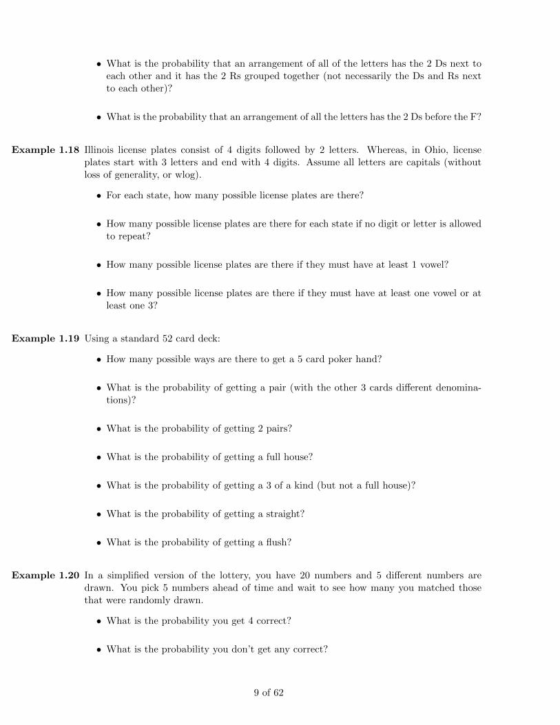
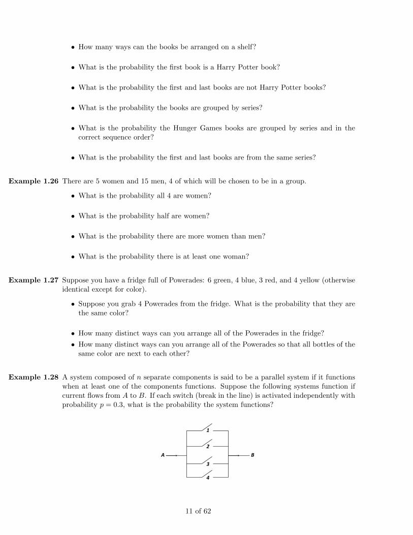
Example 1.28 A system composed of n separate components is said to be a parallel system if it functionswhen at least one of the components functions. Suppose the following systems function ifcurrent flows from A to B. If each switch (break in the line) is activated independently withprobability p = 0.3, what is the probability the system functions?

A B

1

2

3

4

11 of 62

A B

1

2

3

Example 1.29 The U.S. Senate consists of 100 senators, 2 from each of the 50 states. They want to forma committee, where each member has an equal role, consisting of 5 senators.

• How many different committees are possible (without any restrictions)?

• How many different committees are possible if no state can have more than 1 senatoron the committee?

1.6 Conditional Probability, Independence, and Bayes’ Rule

Let A and B be events. The probability that event B occurs given (knowing) that event A occurs iscalled a conditional probability. It is denoted as P(B | A). Whichever event is considered ”given”or ”known” goes after the | in the notation.

P (B | A) =P (B ∩A)

P (A).

The above formula works so long as P(A) > 0. There is an equivalent, within the equally likelyframework, to the above formula. It is

P (B | A) =N(A ∩B)

N(A).

The idea behind conditional probability is that you have an idea of what occurred, but do notknow exactly what happened. Meaning, you can limit the original sample space (Ω) to somethingsmaller. In our above example, we know that the event A occurred, so what we are doing ismaking A our ”new” Ω.

General multiplication rule is defined as

P (A ∩B) = P (A) ∗ P (B | A).

This formula is equivalent to the 2 above, just our goal is different now. Before we wanted tofigure out a conditional probability, now we want to know a joint probability, or a probability ofan intersection of 2 events. This rule can easily be extended to more than 2 events.

P (

n⋂i=1

Ai) = P (A1) ∗ P (A2 | A1) ∗ P (A3 | A2 ∩A1) ∗ ... ∗ P (An | An−1 ∩ ... ∩A1).

12 of 62

Important note: A lot of the formulas in this section are rearrangements of previous formulas.You use one over another depending on what you are given in the problem and what the goal is.

It is important to define 2 types of sampling. Suppose for the sake of argument we are looking atthe integers 1, 2, ... , 10. We want to choose 3 of these numbers, or we have 3 selections. If youwere asked how many ways this could happen, it would depend on if sampling were done with orwithout replacement.

Sampling with replacement means any element of the sample space has the ability to be chosenfor any selection regardless of whether or not it was previously picked. The idea is that no matterhow many selections (or trials) there are, after each selection (or trial), you record the outcome,then put that element back in the population, so that it can be sampled again. In this example,you could pick the number 1 three straight times if sampling were done with replacement. Thiswould be unlikely, but possible.

Sampling without replacement means any element of the sample space has the ability to be chosenat most once. Meaning once you pick an element on a certain selection (or trial), you can neverpick that element again. Again, if you were to make your selection, record the element, you wouldnot put that element back in the population to be chosen again. Once it has been selected, it isno longer a choice for any subsequent selections.

Let us go back to our integer example. How many different samples are possible? If sampling isdone with replacement, we have 10 choices for the first selection. Since we replace our selectionbefore picking again, we still have 10 possibilities for the second selection. Similarly, we have 10options for the last selection. Therefore, we have 10*10*10 = 1,000 different possible samples.

Suppose instead we sampled without replacement. We would still have 10 choices for the firstselection. However, we do not put that element back in the sample space. So, we only have 9available options for our second pick. Additionally, we would only have 8 choices for our lastselection, since we could not use either of our first 2 choices again. In total, we would have 10*9*8= 720 different possible samples.

Example 1.30 Refer to Example 1.15 with Drew. Find the following probabilities:

• What is the probability that Drew drinks something weird, if we know he was paid?

• What is the probability that Drew does something silly, if we know he was paid?

• What is the probability that Drew drinks something weird, if we know he was notpaid?

Example 1.31 (ASW Chapter 4.4, Problem 38) A Morgan Stanley Consumer Research Survey sampledmen and women and asked each whether they preferred to drink plain bottled water or asports drink such as Gatorade or Propel Fitness water (The Atlanta Journal-Constitution,December 28, 2005). Suppose 200 men and 200 women participated in the study, and 280reported they preferred plain bottled water. Of the group preferring a sports drink, 80 weremen and 40 were women. Let

13 of 62

• M = the event the consumer is a man

• W = the event the consumer is a woman

• B = the event the consumer preferred plain bottled water

• S = the event the consumer preferred a sports drink

Answer the following:

• What is the probability a person in the study preferred plain bottled water, or P(B)?

• What is the probability a person in the study preferred a sports drink, or P(S)?

• What is the probability that a person who prefers a sports drink is a man, or P (M |S)?What is the probability that a person who prefers a sports drink is a woman, orP (W |S)?

• What is the probability a person is male and prefers sports drink, or P (M ∩S)? Whatis the probability a person is female and prefers sports drink, or P (W ∩ S)?

• Given a consumer is a man, what is the probability he will prefer a sports drink, orP (S|M)?

Example 1.32 Using the Venn Diagram summarizing the distribution of operating systems (Example 1.13),calculate the following:

• The probability that a randomly chosen student uses all three operating systems, giventhe student uses Windows.

• The probability that a randomly chosen student uses all three operating systems, giventhe student does not use Windows.

• The probability that a randomly chosen student uses Windows, given the student usesMac OS.

• The probability that a randomly chosen student does not use any of the operatingsystems, given the student does not use Windows.

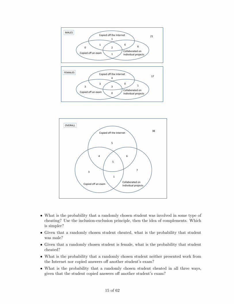
Example 1.33 Case Problem (Adapted from ASW Chapter 9, Case Problem 2, page 397) Cheating hasbeen a concern of the dean of the College of Business at Bayview University for severalyears. Some faculty members in the college believe that cheating is more widespread atBayview than at other universities, while other faculty members think that cheating is nota major problem in the college. To resolve some of these issues, the dean commissioneda study to assess the current ethical behavior of the business students at Bayview. Asa part of this study, an anonymous exit survey was administered to this year’s graduatingclass. Responses to the following questions were used to obtain data regarding three types ofcheating. Any student who answered “Yes” to one or more of these questions was consideredto have been involved in some type of cheating.

• During your time at Bayview, did you ever present work copied off the Internet as yourown?

• During your time at Bayview, did you ever copy answers off another student’s exam?

• During your time at Bayview, did you ever collaborate with other students on projectsthat were supposed to be completed individually?

The data are represented in the following Venn diagrams below:

• Using the law of partitions, fill in the “Overall” Venn diagram.

14 of 62

Copied off the Internet

Copied off an exam Collaborated on Individual projects



MALES

FEMALES

1

1

1

2 6

6 0

4

3

0

3 0

1 3

21

17



OVERALL

5

5

6

7

1

3

4

38

• What is the probability that a randomly chosen student was involved in some type ofcheating? Use the inclusion-exclusion principle, then the idea of complements. Whichis simpler?

• Given that a randomly chosen student cheated, what is the probability that studentwas male?

• Given that a randomly chosen student is female, what is the probability that studentcheated?

• What is the probability that a randomly chosen student neither presented work fromthe Internet nor copied answers off another student’s exam?

• What is the probability that a randomly chosen student cheated in all three ways,given that the student copied answers off another student’s exam?

15 of 62

Example 1.34 Suppose the Queen of Statlandia does not have hemophilia, but may be a carrier of thehemophilia gene. If she is a carrier, any children she has will have a 50% chance of havinghemophilia (independently). If she is not a carrier, her children will not have hemophilia.Since genetic testing is forbidden in Statlandia, the castle physician’s best estimate of theprobability the Queen is a carrier was initially P(carrier)=0.5.

Suppose the Queen has a son, and the son does not have hemophilia. Should the castlephysician’s estimate of P(carrier) change? Why? If yes, to what?

Now suppose the Queen has had three sons (none of which has hemophilia) and would likeanother child. What should the castle physician’s best estimate be for the probability the4th child has hemophilia?

In general, a conditional probability will change the original probability. This change may be anincrease or a decrease. However, it could stay the same. When the conditional probability is thatsame as the unconditional probability, the events are said to be independent. Formally, let A andB be events. Let P(A) > 0. B is independent of A if the occurrence of A does not affect theprobability that event B occurs, i.e.

P (B|A) = P (B).

The special multiplication rule restates the general multiplication rule, but for independent events.If A is independent of B, then

P (A ∩B) = P (A) ∗ P (B).

Use the general multiplication rule to provide a proof of this statement.

Also, the independence of the events A and B implies that the following are independent:

1. AC and B

2. A and BC

3. AC and BC

It would be a good exercise to prove these on your own. For pairwise independence let uslook at the events A1, A2, ..., AN . These events are pairwise independent if for every pair ofevents from the collection, those 2 events are independent of each other. Please note that thisdoes not mean that if you take 3 or more of these events that they are independent. Thatdeals with mutual independence. Again, consider the events A1, A2, ..., AN . They are said tobe mutually independent if for each subcollection of events, the subcollection satisfies the specialmultiplication rule. That is, for each integer n, where 2 ≤ n ≤ N, then

P (Ak1 ∩Ak2 ∩ ... ∩Akn) = P (Ak1) ∗ P (Ak2) ∗ ... ∗ P (Akn),

where k1, k2, ..., kn are distinct integers between 1 and N. Mutual independence implies pairwiseindependence, but not the other way around.

16 of 62

Example 1.35 A man and a woman each have a standard deck of 52 cards. Each draws a card at randomfrom his/her deck.

• Find the probability the man draws the ace of clubs, the woman draws the ace ofclubs, and that they both draw the ace of clubs. Are the 2 events independent? Pleaseexplain why or why not.

• Suppose that 2 people share 1 deck. They each draw from the deck and keep their card.Find the probability the first person gets the king of hearts, the second person gets theking of hearts, and they both get the king of hearts. Are these events independent? Ifnot, what other statistical term represents these two events?

• A person randomly draws from a deck of cards. Let A be the event of a heart, B be theevent of a face card, C be the event of a 7 or Jack. Are the events A and B indepedent?What about A and C? B and C? A, B, and C? Prove your answers mathematically.

Example 1.36 Insurance companies assume that there is a difference between gender and your likelihoodof getting into an accident which is why women generally have lower insurance rates thanmen. We did a study to see the number of accidents that occurred according to gender. Wefound that 60% of the population was male, 86% of the population was either male or gotinto an accident, 35% of the population are accident free. Does this study indicate that thelikelihood of getting into an accident depends on gender? Prove your answer.

Example 1.37 Chris and his roommates each have a car. Julia’s Mercedes SLK works with probability.98, Alex’s Mercielago Diablo works with probability .91, and Chris’ 1987 GMC Jimmyworks with probability .24. Assume all cars work independently of on another. What is theprobability that at least 1 car works?

Law of Partitions: Suppose A1, A2, ..., AN form a partition of the sample space. Then for everyevent B in the sample space,

P (B) = P (B ∩A1) + ...+ P (B ∩AN ).

Furthermore, the law of total probability restates this as

P (B) =

N∑i=1

P (Ai) ∗ P (B|Ai).

A very useful example of this is when you have the simple partition of an event (here we will useE) and its complement. Then,

P (B) = P (E) ∗ P (B|E) + P (EC) ∗ P (B|EC).

Refer to Example 1.37. What is the probability that exactly 1 car works?

Example 1.38 Acme Consumer Goods sells three brands of computers: Mac, Dell, and HP. 30% of themachines they sell are Mac, 50% are Dell, and 20% are HP. Based on past experienceAcme executives know that the purchasers of Mac machines will need service repairs with

17 of 62

probability .2, Dell machines with probability .15, and HP machines with probability .25.Find the probability a customer will need service repairs on the computer they purchasedfrom Acme.

Example 1.39 Let us assume that a specific disease is only present in 5 out of every 1,000 people. Supposethat the test for the disease is accurate 99% of the time a person has the disease and 95%of the time that a person lacks the disease. Find the probability that a random person willtest positive for this disease.

Example 1.40 Polya’s Urn Scheme: An urn contains b black balls and r red balls. One ball is selected atrandom, its color is recorded, and then it as well as c balls of the same color are put backin the urn. this process is repeated. find the probability that the first 2 balls selected areblack and the third ball chosen is red.

Example 1.41 Suppose at a given university the following statements are true. 15% of females are insororities and 18-20% of males are in fraternities. The campus paper uses this informationto claim that 33-35% of campus is ”greek”. Is this correct? If your answer is no, what iswrong with it and how would you fix it?

Example 1.42 A grade school boy has 5 blue and 4 white marbles in his left pocket and 4 blue and 5 whitemarbles in his right pocket. If he transfers one marble at random from his left pocket tohis right pocket, what is the probability of his then drawing a blue marble from his rightpocket?

Bayes’ Rule is used in order to revise probabilities in accordance with newly acquired information.Bayes’ Rule: Let A1, A2, ..., AN form a partition of the sample space. Then for every event B inthe sample space,

P (Aj |B) =P (Aj) ∗ P (B|Aj)∑Ni=1 P (Ai) ∗ P (B|Ai)

.

This is useful when you do not [directly] know the probability of event B, but you know theprobability of B given the events A1, A2, ..., AN . Let us revisit our disease example above (#5).Suppose we are interested in what the probability of having the disease was given that the testwas positive. We now have the following:

P (D|O) =P (D) ∗ P (O|D)

P (D) ∗ P (O|D) + P (DC) ∗ P (O|DC).

This is more often what we are concerned with in this problem. We are concerned with the ideaof having the disease (or sometimes of being pregnant) given that the test was positive. Thisformula takes into account the probabilities of testing positive because the disease is present andthe probability of a false positive.

Let us revisit Example 1.34. What is the probability that the person has the disease giventhat they tested positive?

Refer back to Chris’ car example, Example 1.37. What is the probability that Julia’s car works,given only 1 car works?

18 of 62

Example 1.43 There was an old television show called Let’s Make a Deal, whose original host was namedMonty Hall. The set-up is as follows. You are on a game show and you are given the choiceof three doors. Behind one door is a car, behind the others are goats. You pick a door, andthe host, who knows what is behind the doors, opens another door (not your pick) which hasa goat behind it. Then he asks you if you want to change your original pick. The questionwe ask you is, “Is it to your advantage to switch your choice?”

Example 1.44 Let us roll 2 dice, a hunter green die and a cardinal red die. let A be the event that thehunter green die is odd. Let B be the event that the cardinal red die is odd. Let C be theevent that the sum of the dice is odd. Prove that these events are pairwise independent butnot mutually independent.

Example 1.45 After the first exam, a student will go to the beach (event B) depending on if they pass theexam (event A). The probability a student will pass is .9. If a student passes, they go tothe beach with a probability of .8. However, a student who fails the exam will only go tothe beach with a probability of .4. A student passes the exam with probability .7. What isthe probability that a student at the beach passed their test? What is the probability thata student not at the beach failed the test?

Example 1.46 Suppose you are in MGMT 614, the class is divided into 2 groups and asked to managea portfolio through Yahoo! Finance. On any given day, group 1 has an 85% chance ofincreasing their net worth while group 2 has a 75% chance of increasing their net worth.Assume that they had a decrease if they did not have an increase. Suppose 40% of the classis in group 1. If the teacher picks a student at random to report their portfolio change (fromthe previous day), what is the probability they report an increase? What is the probabilitythat they are from group 2 knowing that they reported a decrease?

Example 1.47 During a tennis match, a player served 75 times. He either aimed at the corner or middleof the court. 60% of the serves were aimed at the corner. Of the serves aimed at the middleof the court, 46.6% were faults (i.e. goodc). Of the serves aimed at the corner of the court,28.8% were faults.

• What percent of serves were good?

• What percent of serves were faults?

• Of the good serves, what is the probability that it was aimed at the corner?

• Of the faults, what is the probability it was aimed at the middle of the court?

Example 1.48 You are playing a game. You get to pick 1 bill out of one of 2 bags. You roll a fair 6-sideddie twice. If the sum is an 8, 9, or 10, you pick from bag B. 80% of the bills in bag A are$5. 72% of the bills in bag B are $5. All the bills are either $5 or $10.

• What is the probability that you get a $5 bill?

• What is the probability you picked from bag A knowing that you picked a $5 bill?

• What is the probability you picked from bag B knowing that you picked a $10 bill?

Example 1.49 An urn originally contains 8 red balls and 2 blue balls. You flip a fair coin 3 times. Foreach head you get, the prizemaster adds 2 more blue balls to the urn. When you are doneflipping the coin, you pull 1 ball from the urn. If you get a blue ball you win a vacation.

• What is the probability that you do not go on vacation?

19 of 62

• Given that you went on vacation, find the probabilities of 0, 1, 2, and 3 heads (sepa-rately).

• Given that you did not go on vacation, find the probabilities of 0, 1, 2, and 3 heads(separately).

Example 1.50 Glen and Jiabai are going to Indianapolis this weekend. They are twice as likely to go onSunday as they are on Friday. They are three times as likely to go on Saturday as they areon Friday. There is a 45% chance of snow on Friday, 25% chance of snow on Saturday, and30% chance of snow on Sunday.

• What is they probability that it snows while Glen and Jiabai are in Indianapolis?

• Given that it did not snow, what is the probability that they went on Friday? Saturday?Sunday?

2 Discrete Random Variables

2.1 General Discrete Random Variables

A variable denotes a characteristic that varies from one person or thing to another. Examples in-clude height, weight, mariatl status, gender, etc. Variables can be either quantitative (numerical)or qualitative (categorical). We use many terms when describing variables, including frequencyand relative frequency. These terms mean “count” and “percent of count written as a decimal”respectively.

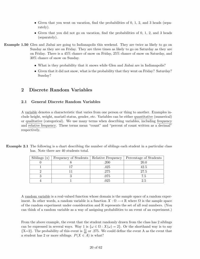
Example 2.1 The following is a chart describing the number of siblings each student in a particular classhas. Note there are 40 students total.

Siblings (x) Frequency of Students Relative Frequency Percentage of Students

0 8 .200 20.0

1 17 .425 42.5

2 11 .275 27.5

3 3 .075 7.5

4 1 .025 2.5

A random variable is a real-valued function whose domain is the sample space of a random exper-iment. In other words, a random variable is a function X : Ω −→ R where Ω is the sample spaceof the random experiment under consideration and R represents the set of all real numbers. (Youcan think of a random variable as a way of assigning probabilities to an event of an experiment.)

From the above example, the event that the student randomly drawn from the class has 2 siblingscan be expressed in several ways. Way 1 is ω ∈ Ω : X(ω) = 2. Or the shorthand way is to sayX=2. The probability of this event is 11

40 or .275. We could define the event A as the event thata student has 2 or more siblings. P (X ∈ A) is what?

20 of 62

There are two main types of quantitative random variables: discrete and continuous. A discreterandom variable often involves a count of something. Examples may include number of cars perhousehold, number of hours spent studying for a test, number of hours spent watching t.v. perday, etc.

A random variable X is called a discrete random variable if the outcome of the random variableis limited to a countable set of real numbers (meaning the r.v. can only take on so many realvalues). Mathematically, we have a countable set K (of real numbers) s.t. P(X ∈ K)=1.

Another key word for r.v.s is support. The word support means the possible values a r.v. cantake. Any r.v. with a countable support – that is whose possible values form a finite or countablyinfinite set – is a discrete r.v. Another way of stating this is to say that all of the probability for adiscrete r.v. occurs at particular points. These points (or numbers) could be 1, 100, .5, -22, - 1

11 .There is no stipulation that a r.v.s’ support must be positive or an integer. Random variables(depending on the context) can take on really any value from R.

Let X be a discrete r.v. Then the probability mass function (pmf) of X is the real-valued functiondefined on R by pX(x) = P(X=x). An important note is that capital letters, like X, are used todenote r.v.s. Lowercase letters, like x, are used to denote possible values of the random variable.This distinction will be used throughout this course as well as in most Statistics courses. Thesubscript in the pX(x) notation is used to denote that this is the pmf of the r.v. X. We could useY, Z, etc. If it is obvious what variable we are referencing, the subscript is often dropped. The xin parentheses refers to the value of the r.v. that we are interested in.

Example 2.2 Flip a fair coin 3 times. Let X denote the number of heads tossed in the 3 flips. Create apmf for X, assuming the following:

• the coin is fair.

• P(heads on 1 flip)=0.7.

• Suppose we used 10 flips, with P(heads on 1 flip)=0.7.

– How many outcomes are there?

– What is the probability of 7 heads?

– What is the probability you get at least one head?

Example 2.3 This is problem 7 from the Fall 2010 Stat 225 Exam 2. There are 3 guys and 2 girls sittingin a row of 5 seats at the Wabash Landing 9. Let G be the number of girls sitting at theends [of the row]. First, find the pmf of G. Secondly, suppose the following information istrue. A person will only order popcorn during the movie if they are sitting at the end ofthe row. A guy will order 2 boxes, but a girl will order 1 box. Let C denote the number ofboxes of popcorn the 5 friends will order. Find the pmf of C.

Example 2.4 Refer to Example 2.1. Let M be the amount of money that parents spend on college. LetM = 30,000(X+1) + 2,000. Find the pmf for M.

Basic Properties of a PMF:

21 of 62

• 0 ≤ pX(x) ≤ 1 ∀x ∈ R. That is to say a pmf is a nonnegative function and it cannot bebigger than 1 at any point.

• x ∈ R : pX(x) 6= 0 is countable. That is the set of real numbers for which a pmf isnonzero is countable.

•∑

x pX(x) = 1. The sum of the values of a pmf equals 1. This is just another way to sayP(Ω)=1.

Suppose that X is a discrete r.v. Then, for any subset A of real numbers, P(X ∈ A) =∑

x∈A pX(x).This states that the probability a discrete r.v. takes a value from a specified subset of real num-bers is just the sum of the pmf of the r.v. over that subset of real numbers.

Interpretation of a pmf In a large number of independent observations of a discrete r.v. X,the proportion of times that each possible value occurs will approximate the pmf at that value.This is the frequentist viewpoint.

Example 2.5 Let X be a random variable with pmf defined as follows. pX(x) = k ∗ (5− x) for x = 0, 1,2, 3, and 4. However, pX(x) = 0 for all other possible values of X.

• Find the value of k that makes pX(x) a legitimate pmf.

• What is the probability that X is between 1 and 3 inclusive?

• If X is not 0, what is the probability that X is less than 3?

Interpretation of an expected value Classic probability asserts that the expected value of ar.v. is the long-run average value of the r.v. in independent observations.

The expected value of a discrete r.v. X, denoted by E[X] is defined by

E[X] =∑x

x ∗ pX(x).

In other words, the expected value of a discrete r.v. is a weighted average of its possible values, andthe weight used is its probability. Sometimes we refer to the expected value as the expectation,the mean, or the first moment. Sometimes it is denoted by µX . For any function, say g(x), wecan also find an expectation of that function. It is

E[g(X)] =∑x

g(x) ∗ pX(x).

An expectation we are often interested in is E[X2]. So, using the above formula, how could wewrite this?

Expectation of r.v.s has some nice properties that can be quite useful computationally. Let X andY be independent, discrete r.v.s defined on the same sample space and having finite expectation(meaning < ∞). Let a and b be real numbers. Then the following hold:

22 of 62

• The r.v. X + Y has finite expectation and E[X + Y] = E[X] + E[Y].

• The r.v. aX + b has finite expectation and E[aX + b] = a*E[X] + b.

The variance of a r.v. is a measure of the spread, or variability, in the r.v. The conceptual defi-nition of variance is Var(X) = E[(X − µX)2]. Basically, this states that variance is the expectedsquared deviation of a r.v. from its mean. You could combine this with the E[g(X)] formulato calculate variance. However, there is another way. We can also define variance by Var(X) =E[X2] - (E[X])2. This is typically more useful, mainly because we are often interested in E[X] sothere is just one more calculation in order to find Var(X).

There are 2 useful properties of variance of a r.v. Let X be a r.v. and let c be a constant.

• Var(cX) = c2*Var(X)

• Var(X + c) = Var(X)

Examples: Refer to Example 2.1, Example 2.2, Example 2.3. Calculate the expectation andvariance of those variables. Please note the properties of expectation and variance. These couldsave you some time. As a check, E[X] and Var(X) for Example 2.1 is 1.3 and .91 respectively.

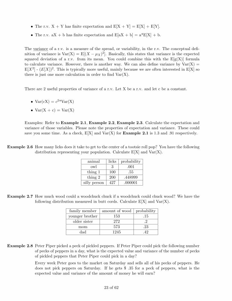
Example 2.6 How many licks does it take to get to the center of a tootsie roll pop? You have the followingdistribution representing your population. Calculate E[X] and Var(X).

animal licks probability

owl 3 .001

thing 1 100 .55

thing 2 200 .448999

silly person 427 .000001

Example 2.7 How much wood could a woodchuck chuck if a woodchuck could chuck wood? We have thefollowing distribution measured in butt cords. Calculate E[X] and Var(X).

family member amount of wood probability

younger brother 153 .15

older sister 272 .2

mom 573 .23

dad 1245 .42

Example 2.8 Peter Piper picked a peck of pickled peppers. If Peter Piper could pick the following numberof pecks of peppers in a day, what is the expected value and variance of the number of pecksof pickled peppers that Peter Piper could pick in a day?

Every week Peter goes to the market on Saturday and sells all of his pecks of peppers. Hedoes not pick peppers on Saturday. If he gets $ .35 for a peck of peppers, what is theexpected value and variance of the amount of money he will earn?

23 of 62

# of Pecks probability

20 .01

50 .25

120 .35

175 .2

200 .19

Example 2.9 Sally sells seashells by the seashore. Suppose on a given day she sells 1-5 shells with respec-tive probabilities .25, .15, .3, .2, and .1. If each shell sells for $2, how much money can Sallyexpect to earn in a day?

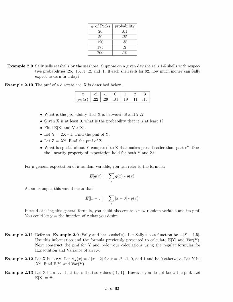
Example 2.10 The pmf of a discrete r.v. X is described below.

x -2 -1 0 1 2 3

pX(x) .22 .29 .04 .19 .11 .15

• What is the probability that X is between -.8 and 2.2?

• Given X is at least 0, what is the probability that it is at least 1?

• Find E[X] and Var(X).

• Let Y = 2X - 1. Find the pmf of Y.

• Let Z = X2. Find the pmf of Z.

• What is special about Y compared to Z that makes part d easier than part e? Doesthe linearity property of expectation hold for both Y and Z?

For a general expectation of a random variable, you can refer to the formula:

E[g(x)] =∑x

g(x) ∗ p(x).

As an example, this would mean that

E[|x− 3|] =∑x

|x− 3| ∗ p(x).

Instead of using this general formula, you could also create a new random variable and its pmf.You could let y = the function of x that you desire.

Example 2.11 Refer to Example 2.9 (Sally and her seashells). Let Sally’s cost function be .4|X − 1.5|.Use this information and the formula previously presented to calculate E[Y] and Var(Y).Next construct the pmf for Y and redo your calculations using the regular formulas forExpectation and Variance of an r.v.

Example 2.12 Let X be a r.v. Let pX(x) = .1|x− 2| for x = -2, -1, 0, and 1 and be 0 otherwise. Let Y beX2. Find E[Y] and Var(Y).

Example 2.13 Let X be a r.v. that takes the two values -1, 1. However you do not know the pmf. LetE[X] = Θ.

24 of 62

• Find a formula for Var(X) written in terms of Θ.

• Verify that your above formula makes sense for when Θ = -1 or for when Θ = 1.

• What value of Θ maximizes Var(X)? Let p be the P(X = 1). What value of p maximizesVar(X)?

Example 2.14 Suppose X and Y are random variables with E(X) = 3, E(Y ) = 4 and V ar(X) = 2. Find:

• E(2X + 1)

• E(X − Y )

• E(X2)

• E(X2 − 4)

• E((X − 4)2)

• V ar(2X − 4)

2.2 Bernoulli and Binomial Random Variables

Many problems in probability involve independently repeating a random experiment and observ-ing at each repetition whether a specified event occurs. We label the occurrence of the specifiedevent a success and the nonoccurrence of the specified event a failure. A success could be afemale child, a head from a coin flip, a 5 on a die, a defective part in a manufacturing warehouse,a green spin in roulette, etc.

A success can take on a positive or negative connotation in the context of an example; it ismerely the event that we are interested in. Each repetition of the random experiment is called atrial. We use p to denote the probability of a success on 1 trial. In Bernoulli Trials, p remainsconstant from trial to trial.

Conditions for Bernoulli:

• The trials are independent of one another.

• The result of each trial is classified as a success or failure, depending on whether or not aspecified event occurs respectively.

• The success probability and therefore the failure probability remains the same from trial totrial.

An important note: Say that we want to extract a sample of size n one-by-one from a largerpopulation, and see how many successes we get. If we sample with replacement, each individualdraw is Bernoulli and all n draws are independent of each other; hence, the number of successesis Binomial. However, if we sample without replacement, the n draws are no longer independent;the distribution of number of successes is no longer Binomial.

Sometimes the Bernoulli Distribution is called an indicator function, i.e. it lets one know whetheror not a specific event has occurred.

25 of 62

Characteristics of the Bernoulli Distribution:

• The definition of X.

• The support is:

• Its parameter(s) and definition(s):

• The pmf if:

• The expected value is:

• The variance is:

We can define the Binomial R.V. as the number of successes in n independent trials, where theprobability of success in one trial is p.Characteristics of the Binomial Distribution:


• The support is:


• The pmf if:



There are several approximations in this course. All 3 of them involve the Binomial in some way.These will be written in later on where appropriate. However, I give a quick summary here. Wecan use the Binomial to approximate the Hypergeometric if N > 20n. We can use the Poisson toapproximate the Binomial if n > 100 and p < .01. We can use the Normal to approximate theBinomial if np > 5 and n(1-p) > 5.

Example 2.15 In Chris’ Stat 225 class, 75% of the students passed (got a C or better) on Exam 1. Ifwe were to pick a student at random and asked them whether or not they passed. Let Xrepresent the number of student(s) who passed.

• What type of random variable is this? How do you know? Additionally, write downthe pmf, the expected value, and the variance for X.

• Repeat under the following assumption: What about if we picked 10 students withreplacement and let X be the number of student(s) who passed.

Example 2.16 Suppose that 95% of consumers can recognize Coke in a blind taste test. Assume consumersare independent of one another. The company randomly selects 4 consumers for a tastetest. Let X be the number of consumers who recognize Coke.

• Write out the pmf table for X.

26 of 62

• What is the probability that X is at least 1?

• What is the probability that X is at most 3?

Example 2.17 To test for ESP, we have 4 cards. They will be shuffled and one randomly selected each time,and you are to guess which card is selected. This is repeated 10 times. You do not haveESP. Let R be the number of times you guess a card correctly. What are the distributionand parameter(s) of R? What is the expected value of R? Furthermore, suppose that youget certified as having ESP if you score at least an 8 on the test. What is the probabilitythat you get certified as having ESP?

2.3 Hypergeometric Random Variables

Important applications are quality control and statistical estimation of population proportions.The hypergeometric r.v. the equivalent of a Binomial r.v. except that sampling is done withoutreplacement, or put another way, the trials are dependent (no longer Bernoulli trials).

As an illustration, let us revisit a poker example. Assume we have a standard 52 card deck andwe are drawing five cards without replacement. Let us use our counting rules to determine theprobability of 3 kings. For the sake of this problem, we are going to assume we do not care whatthe remaining two cards are, just that they are not kings. The answer to this problem involvescombinations since we are sampling without replacement, and the sampling order does not matter(because we only care about which cards we received, not in what order we received them). So,you have to answer 3 questions. How many ways are there to get 3 kings? How many ways arethere to get the remaining 2 cards? How many ways are there total to get a 5 card hand? Put

these all together for the answer of(43)∗(

482 )

(525 ). Little did you know, you just used the hypergeometric

distribution.

Characteristics of the Hypergeometric Distribution:


• The support is:


• The pmf if:



What is the difference between an Binomial r.v. and a Hypergeometric r.v.? Hint: Do NOT sayN.

Approximation. If X∼Hyp(N,n,p) and N > 20n, then we can approximate the probability of Xby using X* ∼ Bin(n,p) (the same n and p).

27 of 62

Example 2.18 There are 100 identical looking 52” TVs at Best Buy in Costa Mesa, California. Let 10of them be defective. Suppose we want to buy 8 of the aforementioned TVs (at random).What is the probability that we don’t get any defective TVs?

Example 2.19 An experiment consists of shuffling a standard deck of 52 cards and then dealing a 10 cardhand. Let Y denote the number of hearts in the hand.

• Identify the distribution of Y and give its parameter(s). Find the probability that Yis 3.

• Suppose instead of using 1 deck, we mix together 1,000 decks. The cards are shuffledand 10 are dealt into a hand. Again, let Y denote the number of hearts in the hand. Isan approximate distribution appropriate for Y, why or why not? Find the probabilitythat Y is 3 (if an approximation is appropriate, use that instead of the exact distri-bution). If you used an approximation, what is the distribution and the value of itsparameter(s)?

Example 2.20 Jacob is shooting a basketball at a carnival in order to win a stuffed animal for his girlfriend.On a single shot, Jacob can make a basket with probability .65. Jacob will win a small prizeif he makes at least 2 out of 3 shots. Jacob pays $4 for three shots.

• What is the probability that Jacob will win a small prize with his first $4. Whatdistribution and what parameter(s) are you using?

•• What is the probability it takes Jacob $20 to win hist first small prize?

2.4 Poisson Random Variables

An important fact from Calculus is: et =∑∞

n=0tn

n! . This fact will allow one to show that the pmffor a Poisson indeed sums to one for any value of λ.

The Poisson r.v. also measures number of successes (like the 3 preceding named discrete r.v.s).However, it is different from the others in the fact that it does not have a sample size (or dependingon perspective, you can take the sample size to be infinite). While our 3 previous r.v.s measurenumber of successes in a certain number of trials, the Poisson r.v. measures number of successesper [blank]. This [blank] can be something like hours, cookies, area, volume, etc. Examples inthe past have included: number of chocolate chips in a cookie (or batch of cookies), number ofbusses per hour, number of silver loop busses per hour, number of defects per square foot, etc.

Characteristics of the Poisson Distribution:


• The support is:


• The pmf if:

28 of 62



Approximation: If X ∼ is Bin(n,p) where n > 100 and p < .01, then X can be approximated byX* ∼ Poisson(λ = np).

Example 2.21 Let us say a certain disease has a probability of occurring in 7 out of 5,000 people. Let ussample 1,000 people. Find the exact and approximate probabilities that 0 people have thedisease and at most 5 people have the disease.

Example 2.22 Suppose earthquakes occur in the western US with a rate of 2 per week. Let X be thenumber of earthquakes in the western US this week. Let Y be the number of earthquakesin the western US this month (assume a 4 week period of time). Find the probability thatX is 3 and Y is 12. Let Z be the number of weeks in a 4 week period that have a week with3 earthquakes in the western US. Find the probability that Z is 4. Is this the same as theprobability that Y is 12? Does this make sense?

Example 2.23 A store has 50 light bulbs for sale. Of these, 5 are black lights. A customer buys eight lightbulbs randomly chosen from the store. Let B denote the number of black light bulbs thecustomer selected. Define the distribution of B. What is the probability that B is 1? Whatis the probability the customer gets at least one black light bulb?

Example 2.24 PRP has on average 4 telephone calls per minute. Let X be the number of phone calls inthe next minute. Find the probability that X is at least 3.

Example 2.25 Customers arrive at the VP on 9th Street at a rate of 10 per hour. What is the distributionof the number of customers that arrive in the first 3 hours, call this distribution Y? Whatis the probability that exactly 12 customers arrive in each of the first 3 hours? What is theprobability that Y is 36?

Example 2.26 You are interested in the Indianapolis Indians. They play 20 games in the month of August.Of their games, they win 10% of them by 2 runs or fewer. Assume each game is independentof any other game. Let G be the number of August games won by the Indians by 2 or fewerruns.

• What is the distribution and parameter(s) of G?

• Wbat is the probability that G is either 2 or 3?

• If the Indians win 4 or more games by 2 or fewer runs in August, they will receive$20,000 bonuses. What is the probability the players receive bonuses?

• Given the players do not receive bonuses, what is the probability that they win exactly3 games by 2 runs or fewer?

• What is the expectation of G?

• What is the variance of G?

Example 2.27 A girl scout troop has 100 boxes of cookies to sell. Of these 100 boxes, 60 are thin mints and40 are Samoas. 10 boxes are randomly selected to be sold at the White County Fair. Let Sbe the number of boxes of Samoas selected to go to the fair. What is the distribution of Sas well as the value(s) of its parameter(s)? Find the probability that S is 0. Suppose thatthin mints can sell for $4 and Samoas can sell for $3.50. What is the expected value and

29 of 62

standard deviation of the amount of money the girl scouts will receive at the fair (assumethat all 10 selected boxes will be sold).

Example 2.28 Tom Maloney decided to hang out with friends the night before his quiz and did not study.He has no knowledge of any of the material on the quiz. The quiz consists of 5 multiplechoice questions with 3 possible answers each. Let T be the number of answers that Tomcorrectly guesses. What is the distribution and parameter(s) of T? What is the probabilitythat Tom gets at least a B (on our grading scale)?

Example 2.29 Flaws on a used computer tape occur on the average of one flaw per 1,200 feet. Let Xdenote the number of flaws in a 4,800 foot roll. Name the distribution of X. What is theprobability that X is at least 1?

2.5 Geometric and Negative Binomial Random Variables

The Geometric and Negative Binomial Distributions also deal with successes and failures. How-ever, they are not looking to count the number of failures in a given sample size. They count thesample size necessary to get a given number of successes. More specifically, if X is Geometric,it measures the number of trials up to and including the 1st success. If X is NB(r,p), then itmeasures the number of trials up to and including the rth success. For both the Geometric andNegative Binomial, we consider the set-up as independent Bernoulli trials.

Characteristics of the Geometric Distribution:


• The support is:


• The pmf if:



The Geometric distribution has 2 wonderful properties. They are called the tail probabiity formulaand the lack-of-memory (or memoryless) property. Their respective formulas are given below:Tail probability: P (X > k) = (1− p)kMemoryless Property: P (X > s+ t | X > s) = P (X > t)

Characteristics of the Negative Binomial Distribution:


• The support is:


• The pmf if:

30 of 62



Example 2.30 Suppose Dunphy is really bad at tossing a Frisbee. His girlfriend attempts to teach him howto aim. However, it inevitably ends in hitting a passerby. Suppose Dunphy hits pedestriansat a rate of 1 out of 5 people that walk past the campus mall. Every time that Dunphythinks he is going to hit a person with the Frisbee, he yells, Geronimo! Eventually, he getsthe hang of it. He exclaims, Eureka! Eureka is Greek for I have found it. However, beforehe gets acclimated to throwing a Frisbee, what is the probability that his first accidentalhitting is between the 5th and 10th person, inclusive, that walks by? What distribution(with parameter(s)) did you use?

Example 2.31 Pat is required to sell candy bars to raise money for the 6th grade field trip. There is a 40%chance of him selling a candy bar at each house. He has to sell 5 candy bars in all.

• What is the probability he sells his last candy bar at the 11th house?

• What is the probability of Pat finishing on or before the 8th house?

Example 2.32 From past experience it is known that 3% of accounts in a large accounting population arein error. (Assume the firm is so big that sampling is done with replacement since samplingthe same account has such as small probability.)

• What is the probability that 5 accounts are audited before an account in error is found?

• What is the probability that the first account in error occurs in the first five accountsaudited?

• What is the probability it takes a double digit number of accounts audited to find onethat is in error?

Example 2.33 Bob is a high school basketball player who has a 70% free throw percentage. Assume all freethrow attempts are independent of one another (i.e. there is no such thing as a hot hand).

• What is the probability it takes more than 3 shots to get his first made free throw?

• What is the probability his first made free throw is on the third shot?

• What is the probability that his third made free throw is on his fifth shot?

• What is the probability that his 100th made free throw is on his 123rd shot?

Example 2.34 The Minnesota Twins are having a bad year. Suppose their ability to win any one game is42% and games are independent of one another.

•• What is the probability it takes 14 games for them to win their fourth game?

• What is the expected value and variance of the number of games it will take them towin their fortieth game?

• What is the expected value and variance of the number of games it will take them towin their first game?

• Knowing they got their 49th win with 5 games remaining in the season, what is theprobability that they do not get 50 or more wins?

31 of 62

To begin with, there are essentially 2 groups of named, discrete random variables that we havediscussed in Stat 225. There are the r.v.s that count the number of successes (Bernoulli, Binomial,Hypergeometric, and Poisson). There are also the r.v.s that count the number of trials up to andincluding a certain number of successes (Geometric and Negative Binomial).

Secondly, Bernoulli and Binomial are related in the sense that Binomial can be thought of as thesum of n independent Bernoulli r.v.s with the same value of p. Or, you could [potentially] thinkof Bernoulli as being a Binomial with n=1.

Thirdly, Geometric and Negative Binomial are related in much the same way that Bernoulli andBinomial are related. Negative Binomial is really the sum of r independent Geometric r.v.s withthe same value of p. Or, you could [potentially] think of Geometric as being a Negative Binomialwith r=1.

Lastly, there are 2 approximations that can be made. The first one occurs if the actual (exact)distribution is Hypergeometric and N > 20n. Then we can approximate it with a Binomial r.v.with the same n and same p as that of the original Hypergeometric r.v. The second approxmationoccurs if the actual (exact) distribution is Binomial and both n > 100 and p < .01. Then, wecan approximate it with a Poisson r.v. where we set λ = np. Why do we do this? Well, we aresetting the expected values equal for the two distributions.

Example 2.35 In a jar there are 200,000,000 coins, 5,000,000 of which are quarters. You select 50 coins fromthe jar randomly and without replacement. Let X be the number of quarters in your sample.What is the distribution of X? Find the probability that X is 2. Is there an approximatedistribution for X, why or why not? If there is, call the approximation X* and find P(X* =2) as well.

Example 2.36 We look at sampling a 5 card hand from a standard deck of playing cards. First, computethe probability of a full house. Nick plays a game with his friend Errrr. Errrr bets $1 everyhand (5 cards). If he gets a full house, he wins $500 (on top of keeping his bet of $1);otherwise, he loses the $1 to Nick. Suppose in an afternoon of gambling, Nick and Eric playthis game 500 times. Let E denote the number of hands that Errrr wins in this particularafternoon. Name the distribution and parameters of E. Find the probability that E is atleast 3. Next, is an approximate distribution appropriate for E, why or why not? If anapproximation is appropriate, label it E* and find the above probability with E* instead ofE.

Example 2.37 Mike is playing fetch with Maxine. At nighttime, Maxine does not always see the ball. Onany one throw, she has a probability of .30 of not seeing/finding the ball. One late autumnevening, Mike throws the ball to Maxine 50 times. Let SM be the number of times thatMaxine cannot find the ball. What is the distribution of SM? Find the probability thatSM is between 13 and 17 inclusive. An approximation is not appropriate for SM, why not?Let’s ignore this and use the approximation anyway. Let SM* be the approximation. Findthe probability that SM* is between 13 and 17 inclusive. Did SM* do a good job?

Example 2.38 Suppose there are 2,000 stocks on the NYSE. We are looking at making a portfolio consistingof 500 different stocks. We just finished reading the Wall Street Journal and discovered that

32 of 62

there are 200 stocks that have risen in price over the last week. Let RS denote the numberof stocks in your sample that have risen over the previous week. What is the distributionof RS? Find the probability that RS is between 50 and 55 inclusive. An approximation isnot appropriate for RS, why not? Let’s ignore this and use the approximation anyway. LetRS* be the approximation. Find the probability that RS* is between 50 and 55 inclusive.Did RS* do a good job?

Example 2.39 Adaptation of Spring 2012 Exam 1 Problem 5. Chris is collecting the quarters featuring thedifferent U.S. states on the back. Suppose now he has a jar with 50 quarters, 7 of which areMinnesota quarters, 8 are Indiana quarters. One day he randomly picks 9 quarters from thejar without replacement. Let MN be the number of Minnesota quarters he selects. Namethe distribution and the parameters for MN. Find the probability that MN is at least 8.Find the probability that MN is at most 2. What is E[MN]?

Example 2.40 Assume the set-up in Example 2.39. However, suppose he picks (with replacement) aquarter until he gets his first one from Minnesota. Let F denote the number of trials ittakes until he picks his first one from Minnesota. Define the distribution of F. Find thefollowing probabilities related to F: at most 4, at least 6, and exactly 5.

Example 2.41 Assume the set-up in Example 8.2. However, now we are looking for the 5th time he picksa Minnesota quarter. Let T denote the number of trials it takes until he picks his fifth onefrom Minnesota. Define the distribution of T. Find the following probabilites related to T:at most 4, at least 6, and exactly 5.

Example 2.42 Adaptation of Spring 2012 Exam 1 Problem 6 Assume a page on a book has to be edited ifthere are at least 2 typos on it. On average, there are 3 typos every 4 pages in this 300 pagebook. Consider pages independent of one another as far as typos are concerned. Let EDrepresent the number of pages that need to be edited in this book. Define the distributionand parameters of ED. Find the following items for ED: expected value, variance, and theprobability it is between 52 and 56 inclusive.

Example 2.43 Assume the set-up in Example 8.4. Additionally, assume that we have 10 books total thathave the same properties as the original book. Let B represent the number of books in thisstack that we have looked at in order to find the first one that has between 52 and 56 pagesthat need to be edited. Create a pmf for B. Let P(B ≥ 10) be P(B=10) in your pmf or pmftable.

Nested problems really just means that we switch distributions throughout the problem. Youmust pay careful attention to the variable under consideration at all times.

Example 2.44 The wonderful candy shop, Albanese Candy Outlet, makes chocolate chip cookies as partof their production line. Chocolate chips in the cookies are randomly and independentlydistributed with an average of 12 chocolate chips per cookie. You and 9 of your friendsdecide to make a trip to Albanese Candy Outlet. Each of you buys one chocolate chipcookie.

• What is the probability that your cookie contains between 10 and 15 chocolate chipsinclusive?

• What is the probability that 5 or 6 people in your group have cookies with between 10and 15 chocolate chips inclusive?

33 of 62

• While examining your cookies (one-by-one), what is the probability that it takes atleast 4 cookies to find the first one with between 10 and 15 chocolate chips inclusive?

• While examining your cookies (one-by-one), what is the probability that it takes atleast 4 cookies to find the first one with 12 or 13 chocolate chips?

• Suppose you and your 9 friends were to go repeatedly to Albanese Candy Outlet. Whatis the probability that it takes until your sixth trip so that 5 or 6 people in your grouphave 12 or 13 chocolate chips in their cookie?

Example 2.45 An urn contains 6 red balls, 6 green balls, and 3 purple balls. You randomly reach in andpull out 4 balls.

• Assume sampling is done with replacement. What is the probability that you draw atleast 2 purple balls?

• Assume sampling is done without replacement. What is the probability that you drawat least 2 purple balls?

• Which of the 2 previous parts was easier computationally and why?

• Assume sampling is done with replacement. What is the probability that it takes youuntil your tenth sample to get a sample with at least 2 purple balls?

Example 2.46 Let us play name the distribution as well as the parameter(s). This problem is adaptedfrom Stat 225 Fall 2008 HW 6 problem 1.

• X is the number of 5’s in ten rolls of a fair die.

• A baseball starting lineup consists of nine players, three of which are outfielders. Arandom sample of three players is taken from a baseball starting lineup. Let X be thenumber of outfielders in the sample.

• X is the number of Hearts in a five-card poker hand dealt from a standard 52 carddeck.

• Let us repeatedly deal out five-card poker hands (replacing the cards after each handis dealt). Let X be the deal number of the first time in which we get a flush.

• Let us repeatedly deal out five-card poker hands (replacing the cards after each handis dealt). Let X be the deal number of the eighth time in which we get a a straight(allow the A-5 straight).

• A player wins a game if he/she rolls at least one 6 in four rolls of a fair die. Let X bethe outcome (win or lose) of this game.

• Customers arrive at Alice’s with a rate of 5 per hour. Let X be the number of customersthat enter Alice’s between 2 A.M. and 4 A.M.

Example 2.47 It rains 3 days per month on average in California. For simplicity assume all months are ofequal length.

• What is the probability that there are no rainy days next month?

• What is the probability that there will be 4 rainless months during the next year?

• What is the probability that April is the first month this year with at least some rain?

• What is the probability that October is the second month with 2 or more days of rainthis year?

34 of 62

3 Continuous Random Variables

3.1 General Continuous Random Variables

A continuous random variable typically involves measurement. One way to define a continuousrandom variable is that it has no point mass, or no point probabilities. This is in direct contrastto discrete random variables. Mathematically, a random variable X is called a continuous r.v. ifP(X=x) = 0 for all x in R. Some useful set notation is that x ∈ (0,1) is x: 0 < x < 1 while x∈ [0,1] means x: 0 ≤ x ≤ 1.

Cumulative Distribution Function, cdf, is a key topic for r.v.s (discrete and continuous alike). LetX be a r.v., then the cdf of X, denoted by FX(x) is the real-valued function defined on R by

FX(x) = P (X ≤ x)

such that x is in R. While a cdf applies to any type of r.v., we typically only use it with respectto continuous r.v.s. The reason for this is that most discrete random variables do not have a nicefunctional form for their cdf.

Example 3.1 Let us find the cdf of a coin tossing example.

• Let n=4, p=.7, and X be the number of heads in the sample. Find the cdf for X.

• Keep the above set-up, but use p=.5 instead. What is the cdf for this r.v.?

Example 3.2 Let us find the cdf of a random experiment over an interval.

• Let X denote a number selected at random from the interval (0,1), what is the cdf ofX?

• Let X denote a number selected at random from the interval (0,10), what is the cdf ofX?

Properties of a cdf

1. It is nondecreasing.

2. It is everywhere right-continuous.

3. It has a value of 0 for x = -∞

4. It has a value of 1 for x = ∞

Useful Identities

• P(c < X < d) = FX(d−)− FX(c)

• P(c ≤ X < d) = FX(d−)− FX(c−)

35 of 62

• P(c < X ≤ d) = FX(d)− FX(c)

• P(c ≤ X ≤ d) = FX(d)− FX(c−)

Most of the above are really important when we have a cdf that has a jump (whether it is a cdffor a discrete r.v. or a “mixed” r.v.). However, the idea of the probability of being in a regionfor a CONTINUOUS r.v. is the cdf at the higher x value minus the cdf at the lower x value.Putting this another way, FX(b−) = FX(b) and FX(a−) = FX(a) for all values of a and b if X isa continuous r.v.

Probability Density Function, pdf is another key topic for continuous r.v.s. Let X be a continuousr.v. A nonnegative function fX is said to be a pdf for X if, for all real numbers a < b,

P (a ≤ X ≤ b) =

∫ b

afX(x)dx

The pdf is the derivative of the cdf (only where the cdf is nonzero. Anywhere the cdf is 0, thepdf is also 0.)

Revisit Example 3.2. What are the pdfs for these 2 problems?

Properties of the pdf:

1. fX(x) ≥ 0 for all real numbers x.

2.∫∞−∞ fX(x)dx = 1.

3. P (a ≤ X ≤ b) =∫ ba fX(x)dx for all real numbers a and b such that a ≤ b.

Recall, item 3 above can also be written as FX(b)− FX(a). This brings us back to the definitionor formulation of the cdf. We can define the cdf in 2 ways. The first is more of the interpretationof the cdf and the second is how to calculate or find it, if it is not given in a problem.

FX(x) = P (X ≤ x)

FX(x) =

∫ x

−∞fX(u)du

Expected Value is still a big topic for continuous r.v.s. The formula is similar to that for discreter.v.s. How do you think the sum would change for a continuous r.v.? How do you think pX(x)would change?

E[X] =

Again, you can do general expectations for functions of a random variable. For any function ofx, say g(x), you can find the expectation of g(x).E[g(x)] =

36 of 62

An interesting note is that not all continuous distributions have a finite expected value (some-times they are infinite). If they do not have a finite expected value, we say they do not have anexpected value. A famous example is the Cauchy distribution, which has a pdf of 1

π(1+x2)which

takes values anywhere in R.

Linearity Property of Expected Value Let X and Y be continuous r.v.s with a joint pdf and finiteexpectations. Also, let a, b, and c be real numbers. Then the following hold:

1. The random variable X + Y has finite expectation and E[X + Y] = E[X] + E[Y].

2. E[cX] = c*E[X]

3. E[aX + bY] = a*E[X] + b*E[Y]

4. E[a + bX] = a + b*E[X]

5. if X ≤ Y, then E[X] ≤ E[Y]

The distribution of a continuous r.v. X is said to be symmetric about a number θ if fX(x− θ) =fX(θ− x) for all values of x. If X is a continuous random variable such that E[X] exists and X issymmetric about θ, then E[X] = θ.

Recall there are 2 different definitions of variance.

V ar(X) = E[(X − E[X])2]

andV ar(X) = E[X2]− (E[X])2

Remember, the first definition is more about the interpretation of variance, and the second defi-nition is usually a bit easier computationally.

Percentiles and Special Percentiles A quartile represents a quarter of a data set or a quarter of a

distribution. There are 3 quartiles of importance to a statistician (1st, 2nd, and 3rd). Sometimesthe first and third quartiles are referred to as the lower and upper quartiles respectively.

• The first quartile, Q1, represents the bottom (lower) 25% of the data.

• The second quartile, Q2, aka the median, represents the bottom (lower) 50% of the data.

• The third quartile, Q3, represents the bottom (lower) 75% of the data.

Q1 is the x value for which FX(x) = .25. You can define similarly Q2 and Q3. A percentilerepresents the lower such-and-such percent of the distribution. For example, the 10th percentilemeans that 10% of the distribution is ≤ that value, or it is the x-value such that FX(x) = .10.You can similarly define any other percentiles. Note: The quartiles are really just special cases ofpercentiles, especially the median.

37 of 62

Example 3.3 Let X represent the diameter in inches of a circular disk cut by a machine. Let fX(x) =c(4x− x2) for 1 ≤ x ≤ 4 and be 0 otherwise. Answer the following questions:

(a) Find the value of c that makes this a valid pdf.

(b) Find the expected value and variance of X.

(c) What is the probability that X is within .5 inches of the expected diameter?

(d) Find FX(x).

(e) What is the 33rd percentile of X?

Example 3.4 Let fX(x) = .25x for 1 ≤ x ≤ 3 and 0 otherwise.

(a) Is X more likely to be within [1,2] or within [2,3]? First answer this question usinglogic. Next, check your answer by calculating the probabilities.

(b) What is the probability that X is more than 2.2?

(c) Find the mean and standard deviation of X.

(d) Find FX(x).

(e) What value of X represents the top 15% of the distribution?

Example 3.5 For each of the following random variables, find their pdfs or cdfs (whichever is missing).

(a)

FX(x) =

0 x < 10

.01(x− 10)2 10 ≤ x < 20

1 x ≥ 20

(b)

FX(x) =

0 x < 0

1− e−λx 0 ≤ x

(c)

fX(x) =

.4 1 ≤ x ≤ 2

.2 3 ≤ x ≤ 6

0 otherwise

Example 3.6 Let X be a continuous random variable with f(x) = c|x− 2| for 1 < x < 4 and 0 otherwise.c is a positive constant. Find the value of c that makes f(x) valid. Find the cdf of X. Whatare the probabilities that X is at most 3, at least 2, between 1.25 and 1.75, and less than 2given it is less than 3? What is the median of X? What is E[X]?

Example 3.7 Let f(x) be c(x+2) from 0 to 1 and c(-x+4) from 1 to 2 and 0 otherwise. Find c. Sketch thepdf. Find the cdf, median, and variance.

Example 3.8 For this problem state whether the given cdf or pdf is valid. If it is not valid, state thereason(s) it is not valid and fix them (adding a constant, multiplying by a constant, changingthe support, ...).

• Let f(x) be (x-2) for x ∈ (1,2+√

3) and 0 otherwise.

• Let F(x) be 0 for x ≤ 1, 2x2 − 3x+ 1 for x ∈ (1,1.75), and 1 for x ≥ 1.75.

• Let F(x) be 0 for x ≤ -3, −3x2+2x+3328 for x ∈ (-3,-1), and 1 for x ≥ -1.

38 of 62

3.2 Uniform Random Variables

Refer back to Example 3.2. It has a uniform characteristic, this applies to its pdf. The UniformDistribution is sometimes said to be evenly or uniformly distributed over an interval. This is agood way to characterize the distribution.Characteristics of the Uniform Distribution:


• The support is:


• The pdf is:

• The cdf is:



Example 3.9 Revisit Example 3.2. These examples are actually uniform distributions. Calculate theexpected values and variances for these 2 distributions. Also, calculate the 41st percentiles.

Example 3.10 Shaggy feeds Scooby a Scooby-snack after every hi-jinks that Scooby foils. Suppose Scoobyfoils a hi-jinks anywhere from 0 minutes into the show up until 15 minutes into the show.Find the pdf, cdf, expected value, and variance for the amount of time until Scooby receivesa Scooby-snack (denoted by X). Additionally, calculate the following probabilities: P(X <5), P(X > 10), P(3 < X < 11), and P(X < 12 | X > 4).

Example 3.11 A very famous, always crowded restaurant named Shenanigans has a porterhouse meal as itsadvertised special on Sweetest Day. It takes between 7 and 16 minutes to cook the porter-house. Find the pdf, cdf, expected value, and variance for the amount of time until yourporterhouse is cooked (denoted by X). Additionally, calculate the following probabilities:P(X < 10), P(X > 12), P(9 < X < 11), and P(X < 14 | X > 11).

Example 3.12 Suppose it takes Landfill between 4 seconds and 15 seconds to finish any given drink. Keep inmind that he has to deal with the noise coming from the glockenspiel. Let X be the amountof time it takes Landfill to finish his next drink. Name the distribution and parameter(s) ofX. Find the probabilities that X is more than 8, less than 12, and between 8 and 12.

Example 3.13 Anywhere from 0 to 20 years a really ridiculous political term gets added to the Englishdictionary. Examples include antidisestablishmentarianism, gerrymandering, and filibuster.What is the probability that the next quirky political term gets added to the dictionarysometime in the next 8 years? What about at least 13 years from now?

3.3 Exponential Random Variables

The Exponential Distribution can be thought of as the continuous analog of the geometric randomvariable. The exponential r.v. is often used as the distribution for the time required to complete a

39 of 62

certain task or for the elapsed time between successive occurrences of a specified event. Addition-ally, the exponential distribution may be used to model the behavior of units that have a constantfailure rate (or units that do not degrade with time or wear out). Some examples include: thetime until an appliance breaks, the time until a light bulb burns out, or the time until the nextcustomer arrives at a grocery store.


• The support is:


• The pdf is:

• The cdf is:



Since the Exponential distribution is the continuous analog of the Geometric distribution, onemight wonder if the 2 great properties from the Geometric also apply to the Exponential. Theanswer is yes. The Exponential also has the memoryless property and a nice tail probabilityformula.

Example 3.14 The sirens, while perched on their aesthetically pleasing fjord, were beckoning for Odysseusto come hither. If it on average takes about 1 minute for a captain to navigate his boatstoward the sirens, what is the probability that Odysseus will steer his ship towards themafter 5 minutes? What is the probability that he takes at most 3 minutes? What is theprobability that it takes between 30 and 90 seconds? What is the probability it takes lessthan 300 seconds knowing it took more than 100 seconds?

Example 3.15 Suppose the time it takes a puppy to run and get a ball, say T, follows an exponentialdistribution with a mean of 30 seconds. State the distribution and parameters of T. Whatis the probability that it takes the puppy more than 50 seconds to get the ball? Assumingindependence, what is the probability that it takes the puppy less than 40 seconds to fetcheach of the next 5 balls? What is the probability that it will take the puppy more than 45seconds to get the ball knowing that it took the puppy longer than 20 seconds?

Example 3.16 You and 3 friends decide to drive from West Lafayette to Boston to watch the Patriots lose.The duration of a round trip, say D, has an exponential distribution with a rate of 1 tripper 20 hours. Find the following probabilities: D is at most 15 hours, D is between 15 and25 hours, D exceeds 25 hours, and D is at most 40 given that it is more than 15. Lastly,calculate the mean and variance of D.

3.4 Poisson Processes

For a specified event that occurs randomly in continuous time, an important application of prob-ability theory is in modeling the number of times such an event occurs. The following are severalexamples of such random phenomenon.

40 of 62

• The number of patients that arrive at a hospital emergency room.

• The number of customers that enter a particular bank.

• The number of accidents at an intersection.

• The number of alpha particles emitted by a radioactive substance.

Consider an event that occurs randomly and homogenously in continuous time at an average rateof λ per unit of time. We will refer to the occurrence of the event as a success. If we begincounting successes at time 0, and, for each time, t ≥ 0, we let N(t) = the number of successesby time t (≤ t). Automatically, this implies that N(0) is 0. We say such a counting process is aPoisson Process with rate λ if 2 more properties hold. Namely, if:

• N(t): t ≥ 0 has independent increments (as long as the two time intervals have no overlap,they are indepedent).

• N(t) - N(s), which is the number of successes in the time interval (s,t], is distributed asPoisson(λ(t-s)) for 0 ≤ s < t < ∞.

As indicated by previous examples, the Poisson Process can be used to model arrivals. It is alsoused for waiting times and interarrival times.

For each n ∈ N, we let Wn denote the time of the occurance of the nth event. That is the timeat which the nth success occurs. If W3 is 10.34, that means the 3rd success occurred at a timeof 10.34. The random variable Wn is called the nth waiting time. The elapsed time between theoccurrence of the (n− 1)st and nth events is denoted by In and is called the nth interarrival time.So, we have the following 2 relationships:

Wn =n∑j=1

Ij

In = Wn −Wn−1

One nice property of a Poisson Process with rate λ is that the interarrival times, or Ins are iidExponential random variables with rate parameter λ.

There is one more property of a Poisson Process that is quite useful. Suppose we have Wt =n. This means that we had n successes on the interval [0,t]. These successes are independentUniform(0,t) random variables. Keep in mind that time increments are independent for a Poissonrandom variable if there is no overlap. Knowing Wt = n, if we looked at the distribution of thenumber of successes on the interval [0, t4 ], how would these be distributed?

Example 3.17 Suppose that phone calls arrive at a switchboard according to a Poisson Process at a rateof 2 per minute. Let X be the number of calls between 9:30 and 9:45. Find the distribution

41 of 62

of X. Let T be the time between the 8th and 9th calls. What is the distribution of T? Whatis the probability that exactly 10 calls (total) come in the next 4 minutes? What is theprobability that the next call comes in 30 seconds and the second call comes at least 45seconds after that? Given there are exactly 7 calls in 3 minutes, what is the probabilitythat they all came in the last minute?

Example 3.18 Each time a student logs on to their ITaP account, the computer sends a request for thestudent’s profile to the main ITaP database. Suppose that these profile requests come tothe main database according to a Poisson Process at a rate of 9 per minute. What is theprobability that between 8 and 11 (inclusive) profile requests go to ITaP in a given minute?On average, how many profile requests arrive in an hour period? What is the probabilityof 7 profile requests in a 1-minute interval followed by 19 profile requests in the subsequent2-minute interval? How long, on average, does it take between successive profile requests?What is the probability that the next profile request takes more than 15 seconds? What isthe probability that the next profile request takes at most 22 seconds? It we know that 13profile requests occurred between 12:00:00 AM and 12:01:30 AM, what is the probabilitythat 5 profile requests occurred between 12:00:50 and 12:01:20?

Example 3.19 Customers arrive at Scotty’s at a rate of .5 per minute. (Assume all customers arriveindependently of all other customers.) What is the probability that 10 customers arrive inthe next 15 minutes? What is the probability that 10 customers arrive in each of the next4 15-minute intervals? How long on average does it take for the next customer to arrive?What is the probability that I1 is more than 20 seconds, I2 is more than 30 seconds, and I3is less than 15 seconds?

Example 3.20 At any point during a Stat 225 exam, the next person to drop a calculator will take 5minutes on average to do so. Let C represent the time until the next person drops theircalculator. Name the distribution and parameter(s) of C. Find the following probabilities:C is more than 5 knowing that it is less than 10, C is at least 8 given it is less than 15, Cis more than 2, C is less than 4, and C is at least 7 given that it is more than 5.

Example 3.21 Purdue undergraduate students’ IQ are evenly distributed over the interval 80 to 170. Pick arandom undergraduate from Purdue. Let I denote their IQ. Find the following probabilities:I is less than an ”average” intelligence (100), I is more than 130, I is between 110 and 140,and I is more than 90 given it is less than 120. Also, in order to be in Mensa, a person mustbe in the top 2% of all IQs. What is the top 2% IQ score for a Purdue undergraduate?

Example 3.22 Suppose that the amount of time one spends in a bank has a mean of 10 minutes. Let T bethe amount of time that Glen spends in his bank. What are the following probabilities: Tis more than .25 hours, T is less than .2 hours, T is less than .25 hours given it is at least.16 hours? Find the 40th percentile of T.

Example 3.23 Shoe sizes of NBA players are equally likely over the interval 14 to 22. Let S represent theshoe size of a random NBA player. Find the following: the 10th percentile of S, the value ofS such that only 12% of NBA players have bigger feet, the probability that S is between 10and 16, the probability that S is more than 17, the expected value of S, and the variance ofS.

Example 3.24 Let X ∼ Expo(λ = 2). Find P(X < 4), P(X > 1.2), and Var(X).

Example 3.25 Thomas is examining a length of television wire for defects. He knows that there are anaverage of 3 defects in every 10 feet of wire, that the occurrence of defects in any segment

42 of 62

of wire is independent of the occurrence of defects in any other segment, that all segmentsof wire are equal with regards to the occurrence of defects, and that for sufficiently smallsegments of wire the likelihood of finding more than one defect is practically zero. Let D1

be the number of defects in the first 10 feet of wire, D2, be the number of defects in 50 feetof wire, W be the amount of wire between the fifth and sixth defects. Find the followingprobabilities: D1 is between 2 and 4 inclusive, there are multiple defects in the first 10 feetof wire, D2 is 15 or 17, W is at most 3, W is at least 2, W is at most 10 given it is at least7.

Example 3.26 Find the expected value and variance of the 3 variables defined in Example 3.25. SupposeMike is supervising Thomas. He inspects Thomas’ work right before lunch. This coincideswith feet 30 through 45 of the wire. It is known that Thomas finds 6 defects while Mike iswatching. Let Y be the number of these defects that occur anywhere from the 38th foot tothe 42nd foot. Find the following probabilities for Y: it is at least 1, it is at most 2. Supposefurther that we know no defects occured in the last 3 feet of wire (from the 42nd foot to the45th foot). Recalculate the previous 2 probabilities.

Example 3.27 Suppose Lynda Thoman arrives to her office on Monday’s anywhere from 6:45 AM to 7:45AM and that she is equally likely to arrive anywhere in that interval. Let T be the timeof her arrival. Find the following probabilities for T: it is between 7 and 7:30, it is at most7:25, it is at least 7:30, it is less than 7:40 knowing it is more than 7:20. Also, find E[T] andVar(T).

Example 3.28 Refer to Example 3.27. It is known that she teaches at 7:30 AM on Monday’s. It is alsoknown that it takes her 12 minutes to walk from her office to where she teaches, and it takesher 8 minutes to make a pot of coffee. Find the following probabilities: she is late to classknowing she did not make coffee, she is late to class knowing she made coffee, she is on timeto class and had at least 11 minutes in her office, she is on time to class and had at least11 minutes in her office to enjoy the coffee that she made. Lastly, knowing that she was ontime to class, what is the 23rd percentile of the time that she arrived to her office (writethis as a time).

Example 3.29 The time that it takes until a student uses a cell phone in class is exponential with a meanof 1.1 minutes. Marıa just used her cell phone at 12:55 PM. Let X be the time until thenext person uses a cell phone. Class ends at 1:00 PM. Find the following probabilities: X isat most 2.3, X is more than 3.9 knowing it is more than 2.3, that no one uses a cell phoneuntil after class is over. What is the 81st percentile of X (write this as a time)?

3.5 Normal Random Variables

One of the most important distributions in Probability and Statistics is the Normal Distribution.Any Normal distribution problem will be labeled as a Normal Distribution. Let us start with the

pdf of the Normal. It is: fX(x) = 1√2πσ

e−(x−µ)2

2σ2 for any real number x, any positive number σ, and

any real number µ. Now, you know the pdf, support, and parameters for a Normal Distribution.Take a minute to calculate the cdf of the Normal.

A potential next question is what do µ and σ mean (or represent)? The answer shall be providedby your teacher. This also eliminates the typical 6th and 7th bullet points for your distributions.

43 of 62

Thus completing all 7 bullet points.

A Normal Distribution is sometimes referred to as a bell curve because of how the pdf looks.One important property of this bell curve is that it is symmetric. What is a Normal Distributionsymmetric about? While talking about the shape of the pdf, what would happen to the graph ofthe pdf if we changed σ? What about if we changed µ?

One drawback of the Normal Distribution is that its cdf is not a simple algebraic formula. Thereis no closed form solution to the cdf of a Normal. Therefore, in order to find any probabilityassociated with a Normal(µ, σ2) random variable we need to do an algebraic trick that is calledstandardizing a Normal r.v. To understand this concept, first we need to introduce the variableZ. In Statistics, Z is reserved for a Normal(µ = 0, σ = 1) random variable. Z is referred to as theStandard Normal. Our ”trick” is to turn a Normal(µ, σ2) into a Normal(µ = 0, σ = 1) randomvariable. This is done by the following formula:

Z =X − µσ

.

Unlike other continuous random variables, the pdf and cdf for Z are not labeled with f and F.Instead, they are labeled with φ and Φ respectively. Because of the importance of Z in Statistics,it gets its own letter to represent its pdf and cdf. However, since Z is a Normal r.v. its cdf doesnot exist in closed form either. Instead, we have a table of probabilities. The one we will use inthis course is on the course web site as ”Normal Table”. Please print this pdf off and bringit with you to every class.

If X is a Normal(µ, σ2) r.v., then P(c < X < d) = Φ(d−µσ ) - Φ( c−µσ ). In other words, we canrelate the cdf of X to the cdf of Z. FX(x) = Φ(x−µσ ). Recall that a Normal r.v. is symmetric.This actually implies the following: Φ(−z) = 1− Φ(z). This is useful for P(Z ≥ z) = 1 - Φ(z) =Φ(−z).

Now that we can calculate probabilities for a Normal r.v., there are 2 other main topics to dis-cuss. The first is about sums of independent Normal random variables. Let Xi denote mutuallyindependent Normal random variables with parameters µi and σi respectively. Their sum hasmean equal to the sum of the µi and variance equal to the sum of the variances. If we let Y =∑n

i=1Xi then Y ∼ Normal(µy =∑n

i=1 µi, σ2y =

∑ni=1 σ

2i ). This can be applied to any number

of Normal random variables (provided that they are mutually independent). (Quick aside: Thisprovides motivation for the CLT, which a lot of you will see in MGMT 305.)

Example 3.30 Let us examine Z. Find the following probabilities with respect to Z: at most -1.75, at most1.75, between -2 and 2 inclusive, less than .5. Find the following with respect to Z: the valuesuch that 20.3% are higher than it, the 4.65th percentile, and the values representing themiddle 96.6% of the distribution.

Example 3.31 Let X be Normal with a mean of 20 and a variance of 49. Find the following probabilities:X is between 15 and 23; X is more than 12 knowing it is less than 20; given X is less than28, the probability that it is more than 16; and that it is more than 31. What is the valuethat is smaller than 20% of the distribution?

44 of 62

Example 3.32 Let X1, X2, and X3 be mutually independent, Normal random variables. Let their meansand standard deviations be 3k and k for k = 1, 2, and 3 respectively. Find the followingdistributions:

∑3i=1Xi, X1 + X2 - X3, 2X1 - 3X3 + 4X3. Call the previous distributions

S, T, and V respectively. Find the following percentiles for S, T, and V respectively, 83th,63rd, and 42nd. Find the following probabilities: S is bigger than V’s mean, T is smallerthan half of S’s variance, and V is bigger than T’s 99th percentile.

Example 3.33 SAT Math scores follow a Normal distribution with a mean of 533 and a standard deviationof 116. Assuming that scores above 800 get truncated to 800, what percent of scores werereported as 800? The middle 50% of SAT Math scores at Purdue in 2011 were reported as550 to 690. What percent of all SAT Math scores were in this range? Notre Dame’s middle50% are between 680 and 770. What percent of all scores are below Notre Dame’s 75th

percentile? What percent of all scores are above Notre Dame’s 25th percentile?

Example 3.34 Colin and Mike are wasting their childhood playing ping pong in Colins basement. Sincethey have spent so much time in the basement playing ping pong, pool, and darts, they arefamished. They decide to order Chinese food with extra teriyaki sauce for delivery. If thefood will arrive according to a normal distribution with mean of 20 minutes and standarddeviation of 5 minutes, what is the probability that the two kids have to wait more than 32minutes for their food? What is the probability that they wait less than 15 minutes? Whatis the probability that they wait less than 26 minutes, knowing that they wait at least 12minutes?

Example 3.35 Suppose you and 4 of your best friends are migrating west. You are the local physician.Suppose you decide to hunt buffalo. On average buffalo have 800 lbs. of edible meat witha standard deviation of 75 lbs. If your party comes back to the trail with one buffalo, whatis the probability that you come back with less than 700 lbs. of edible meat? If you need925 pounds of edible meat to make it all the way to Independence, Missouri, what is theprobability that your 1 buffalo will last you until Independence, Missouri? What amount ofedible meat is less than 29% of the distribution?

Example 3.36 “Wish” by NIN is a 3 minute and 36 second long song. Suppose the length of time thepyrotechnics last is normally distributed with an average of 2 minutes, and they have astandard deviation of 53 seconds. Suppose NIN use pyrotechnics at the beginning of “Wish”.What is the probability that the fog will still mask Trent Reznor at the end of “Wish”?

Example 3.37 A male yeti’s height is normally distributed with a mean of 84 inches and a standarddeviation of 7 inches. Since, yetis seem to elude people, we will not make a question aboutthe probability of a specific yeti, but of yetis in general. What are the 25th, 48th, and 67th

percentiles for height of a yeti?

We can use a Normal Distribution to approximate a Binomial Distribution if n is large and p ismoderate (close to .5). Our rule of thumb for this approximation to be valid is that both np >5 and n(1-p) > 5. If X ∼ Binomial(n,p) and the approximation holds, then the approximation,X* ∼ N(µ = np, σ2 = np(1-p)). One caveat to this approximation is that we are approximatinga discrete distribution (the Binomial) with a continuous distribution (the Normal). One thingthat we know about these types of distributions is that discrete r.v.s have point probabilities,but continuous r.v.s do not. In order to account for this, we use the continuity correction. Thisinvolves either adding or subtracting a half from the x value accordingly.

45 of 62

A Normal Distribution is sometimes referred to as a bell curve because of how the pdf looks.One important property of this bell curve is that it is symmetric. What is a Normal Distributionsymmetric about? While talking about the shape of the pdf, what would happen to the graph ofthe pdf if we changed σ? What about if we changed µ?

The Empirical Rules or as they are sometimes known the Rules of Thumb are a way to ap-proximate certain probabilities for the Normal Distribution. There are 3 rules of thumb and theycontain two parts: an interval and a percent (or probability).

Interval Percent Contained

µ± 1 ∗ σ 68%

µ± 2 ∗ σ 95%

µ± 3 ∗ σ 99.7%

The above intervals are all centered around µ. Additionally, since the Normal Distribution iscentered around µ, these intervals represent the middle 68, 95, and 99.7 % of the Normal Distri-bution. Recall that the Normal Distribution is symmetric. This means that the % not includedin each interval is equally distributed on the low and high ends of the interval. For example, thatmeans 16% of the distribution is < µ− 1 ∗ σ.

Example 3.38 Mr. DeFries’ golf scores per 9 holes ar Normally distributed with a mean of 50 strokes and avariance of 25 strokes. For this entire problem, use the Empirical Rules. Find the probabilitythat Mr. DeFries scores between 45 and 60 on his next round. Find the probability thatMr. DeFries scores between 55 and 65 on his next round. Find the probability that Mr.DeFries scores less than 55 on his next round. What is the 97.5th percentile of his scoredistribution?

Example 3.39 NFL players height is Normally distributed with a mean of 74 inches and a standard devi-ation of 2 inches. For this entire problem, use the Empirical Rules. The middle 95% of allNFL players have heights between what 2 values? Find the .15th percentile.

Example 3.40 For this entire problem, please use the Rules of Thumb. The number of pairs of shoes inan adult female’s closet is Normal with a mean of 58 and a standard deviation of 5. Whatinterval contains the middle 68% of the distribution? Find the value such that 2.5% arelower than that value. What is the probability an adult female’s closet has between 48 and63 pairs of shoes? What percent of adult women have between 68 and 73 pairs of shoes intheir closet?

Example 3.41 Suppose a class has 400 students (to begin with), that each student drops independently ofany other student with a probability of .07. Let X be the number of students that finish thiscourse. Find the probability that X is between 370 and 373 inclusive? Is an approximationappropriate for the number of students that finish the course? If so, what is this distribu-tion and what are the value(s) of its parameter(s)? For the following probabilities, if anapproximation is appropriate, use the approximation; otherwise, use the exact distribution.Find the probability that is between 370 and 373 inclusive, that X is at least 375, that X isat most 370, that X is between 360 and 380, and that X is between 360 and 380 inclusive.

46 of 62

Example 3.42 Brian is a movie buff. He has an enormous DVD collection, that he lets his friends borrowfrom. Let N represent the number of DVDs that Brian has in his house at any given time.N is Normal with a mean of 600 and a variance of 144. Find the following probabilities: N iswithin 20 of its mean, N is greater than 630, N is less than 560, N is greater than 588 or lessthan 624 but not both. (Please answer the next 2 questions with an unrounded answer anda rounded answer.) What is the 34th percentile of N? What number of movies representsthe top 15 percent for N?

Example 3.43 Clayton, Jeremy, and Eric are at Balmoral Race Track betting on horses. The 7th race has8 horses. A Trifecta requires you to pick the first 3 horses (win, place, and show) in order.A Box around a Trifecta (or a superfecta for that matter) means that you do not have topick the order, only the horses that are in the first 3 spots. Suppose they pool their moneyand buy 400 $1 Boxed Trifectas for the 7th race and they pick the horses at random for eachbet. Suppose each bet costs $6 (why would that make sense?) and that a winning ticketpays $500. Let X represent the number of winning tickets. Find the following probabilities:X is 7 or 8, they have at least 1 winning ticket, they make money on this bet. Lastly, whatis the expected value and variance of their profit from this bet?

Example 3.44 Refer to Example 3.43. Is an approximation appropriate for X? Justify your answer. If itis, recalculate the probabilities using the approximation.

Example 3.45 Karl is making some pasta and will let it boil between 8 and 10 minutes before removingfrom the stove and draining. Let X be the length of time the pasta will boil on the stove.What is the distribution of X? Find the following probabilities: X < 8.8, X > 9.4, X isbetween 8.75 and 9.1, and X is greater than 8.4 given that it is smaller than 8.95.

Example 3.46 Kathy has decided to Go Green and is replacing all existing lights in her apartment withenergy saving bulbs. These new energy saving bulbs have a mean lifetime of 7 years. LetX be the amount of time until she needs to replace one of these new bulbs. What is thedistribution of X? Find the probability that X is: more than 5 years, at most 10 years,between 2 and 6 years, greater than 12 given it is greater than 8, greater than 3 given it isless than 7.

Example 3.47 At a STAT Christmas party, Ritabrata claims that he can accurately identify the contentsof a wrapped present 45% of the time, with each package independent of any other. LetX be the number of presents Ritabrata correctly identifies in the 16 packages at the party.What is the distribution of X? Is the an appropriate approximation for X (why or whynot)? Find the probability that X is: 8, at least 14, and at most 4. If an approxmation wasappropriate, state the approximate distribution and repeat the probability calculations.

Example 3.48 The length of Dougs 225 lectures follow a Normal distribution with an average of 47.5minutes and a standard deviation of 1.25 minutes while Grant’s 225 lectures follow a Normaldistribution with an average of 49.25 minutes and a standard deviation of 0.75 minutes.Assume the length of a 225 lecture is independent from day to day and between TAs. Whatis the probability that Doug lectures longer than the median time that Grant lectures?Grant wants to reassure his students by telling them that he will only lecture longer than”M” minutes 8% of the time. Find ”M”. Classes are 50 minutes long, what is the probabilitythat at least 1 TA will let their students out late.

Example 3.49 Chester is on vacation with his wife and children. They go to a restaurant where the specialis a 96 ounce steak. The restaurant will give you a gift card worth 4 free meals if you canfinish this steak. It is known that only 10% of all people that attempt this challenge will

47 of 62

actually be able to finish this giant steak. The week before Thanksgiving, several peopleattempt this challenge to try and prepare for their Thanksgiving feasts. Suppose that 200people attempted to eat the 96 oz. steak during this week. The proportion of people thatwill successfully finish the steak is ∼ N(µ = .1, σ2 = .00045). Find the following probabili-ties: more than 26 people finished the steak and at most 40 people finished the steak. Howmany people do you expect to finish the steak?Suppose this set-up applies during every Thanksgiving week. The top 18% of all Thanks-giving weeks have at least how many people finish this steak? The bottom 31% of allThanksgiving weeks have at most how many people finish this steak?

Example 3.50 The number of trick or treaters (labeled tots hereafter) that arrive at Harvey’s house areequal over time with a mean of 7 per hour. Assume all tots arrive independently of oneanother. Find the following: 8 tots in the first hour, 12 tots in the first 2 hours, 8 tots inthe first hour and 12 tots total in the first 2 hours, it takes more than 5 minutes for thenext tot to show up, and the probability that 10 tots show up in the first 1.5 hours if 20tots showed up total (a 4 hour period).

Example 3.51 Let X be a continuous random variable. Let the pdf of X be c(3x2 − 2x) for x between 2and 4 inclusive. First, find the value of c that makes this a legitimate pdf. Second, find thecdf. Additionally, find E[X], Var(X), the median, the probability X is at most 3, and theprobability X is between 2.3 and 3.1.

4 Numerical Summaries

4.1 Quantitative Random Variables

Sample statistics are numerical measures of location, dispersion, shape, association, etc. thatare computed for data FROM A SAMPLE.

Population parameters are numerical measures of location, dispersion, shape, association, etc.that are computed for data FROM A POPULATION.

Note: most of the time, we will just say statistic or parameter. Keep in mind that statistics are al-ways from the sample and parameters are always from the population. In most cases, parametersare denoted by Greek letters, and statistics are denoted by their English alphabet counterparts.Additionally, sometimes statistics are referred to as point estimates of the parameter that theyrepresent. This concept is especially prevalent during hypothesis testing and confidence intervalconstruction.

Mean is the average value or expected value. The population mean is represented by mu, µ.If necessary, you can add a subscript to avoid confusion, like µx vs µy. The sample mean isrepresented by x-bar, x.

Computation of x:

48 of 62

The population variance is denoted as σ2, while the sample variance is denoted by s2. Theyare computed as such:

Mode is the value that occurs the most (has the highest frequency).

Range = largest value (maximum) - smallest value (minimum).

Percentile is best represented with an example. The pth percentile is a value of the data set (ordistribution) such that at least p% of the data set (or distribution) is ≤ this value. There are 3special percentiles, call the quartiles. The quartiles split the data into 4 parts. The lower quar-tile, median (aka the 2nd quartile), and the upper quartile are the 25th, 50th, and 75th percentilesrespectively. The lower and upper quartiles are sometimes known as the first and third quartiles.We typically abbreviate these 3 values as Q1, M, and Q3.

Calculation of Percentiles (and Quartiles) using the indexing method (see page 86 of Statisticsfor Business and Economics by Anderson, Sweeney, and Williams, 11th ed. ).:

Interquartile Range, or IQR is Q3 - Q1.

A boxplot is a visual representation of the 5 number summary. The 5 number summary is theminimum, Q1, the median, Q3, and the maximum. Boxplots have different types. Namely, thereis a ”regular” boxplot and a modified boxplot. The modified boxplot will highlight if there areoutliers, but a regular one will not. Your teacher will demonstrate both of these versions. Pleasekeep in mind that there are different variations of a modified boxplot.

An outlier is a data point that does not fit with the rest of the data. In a univariate case, thisnumber can be either too small or too large. In a bivariate case, it would be a data point thatdoes not fit the overall trend of the variables taken together. Here is our outlier test:

Example 4.1 Hank Aaron hit an astounding 755 home runs in his career. His career spanned from 1954through 1976. In those 23 seasons he hit 13, 27, 26, 44, 30, 39, 40, 34, 45, 44, 24, 32, 44,39, 29, 44, 38, 47, 34, 40, 20, 12, 10. What is the mode of the data set? What is the rangeof the data set? Create both a regular and a modified boxplot for the number of home runsthat Hank Aaron hit in a season. Find the 61st percentile.

Example 4.2 A Stat 113K class was asked how many times they wanted to eat ice cream last summer.The answers given were: 0, 15, 18, 7, 15, 28, 10, 20, 3, 10, 6, 10, 8, and 9. What is themode of the data set? What is the range of the data set? Create both a regular and amodified boxplot for the number of times the students wanted to eat ice cream.Find the18th percentile.

Example 4.3 Suppose we have the data set 1, 2, 3, 4, and 5. Find the mean of the data. Also computevariance in 2 ways (one assuming that this is a sample, the other assuming that this repre-sents the entirety of the population). For these 2 different variance calculations, how would

49 of 62

you denote the mean?

Example 4.4 Suppose we have the data set -4, -2, 0, 2, and 4. Find the mean of the data. Also computevariance in 2 ways (one assuming that this is a sample, the other assuming that this repre-sents the entirety of the population). How does the variance relate to that in example 13.3?Is this suprising or can you show why this is true?

Statistics is the science of collecting, analyzing, presenting, and interpreting data.

Data are the facts and figures collected, analyzed, and summarized for presentation and inter-pretation.

Data set all the data collected in a particular study.

Elements are the individual entities of a data set.

A variable is a characteristic of interest for the elements.

An observation is the set of measurements obtained for a particular element.

4.2 Qualitative Random Variables

There are two main types of variables, qualitative (aka categorical) and quantitative (aka numer-ical).

Qualitative data has labels or names used to identify an attribute of an element. Qualitativedata use either the nominal or ordinal scale of measurement.

Nominal scale is such that order does not matter.

Ordinal scale is such that order does matter. The order or rank of the data is meaningful.

Quantitative data has numeric values that indicate how much or how many of something.Quantitative data uses either the interval or ratio scale.

Interval scale has ratios of quantities that cannot be compared.

Ratio scale has ratios of quantities that are meaningful.

50 of 62

Note: We can use numeric values to represent categoric data. This is often done when workingwith a data set. For example, suppose we are interested in grade level of a student. Instead ofusing the values of Freshman, Sophomore, Junior, and Senior, we could use the values 1, 2, 3, and4. Since the numbers represent categories, grade level is a qualitative variable.

When referring to a variable, we can describe it is qualitative or quantitative, and one of nominal,ordinal, interval, or ratio.

Cross-sectional data is data collected at the same or approximately the same point in time.

Time series data is data collected over several time periods.

Example 4.5 Wabash College student data set

Gender Grade Hometown Major Pieces of Candy Consumed

Male Sophomore Indianapolis Psychology 15

Male Senior Crown Point Spanish 12

Male Senior Lombard Religion 8

Male Freshman Indianapolis Philosophy 10

• What is the entire spreadsheet of data called?

• Each student is what?

• How many elements are in the data set?

• How many variables are in the data set?

• List the 3rd observation.

• What type of variable is each variable in the data set (be sure to answer both qualitativeor quantitative as well as nominal, ordinal, interval, or ratio).

Example 4.6 For this example, answer what type of variable each of the following are (be sure to answerboth qualitative or quantitative as well as nominal, ordinal, interval, or ratio). Smokingstatus, SAT score, income, level of satisfaction, GPA, clothing size (s, m, l, xl), and timetaken to run a mile.

Example 4.7 For this problem, state whether the variables included are cross-sectional or time series.

• Current GPAs of Purdue Statistics Graduate Students vs. GPA of Sanvesh during histime at Purdue.

• Value of Gordan Gecko’s portfolio over the previous 3 years vs. Value of all portfolio’sat Charles Schwaab in January 2008.

• Total salary of the LA Lakers throughout the 1990s vs. Salaries of all NBA teams in1994.

51 of 62

4.3 Sampling

Where does data come from? Sources of data can be existing sources (employee records, studentrecords, medical history, etc.), surveys (teacher evaluations, amazon buyer reports), experiments,or observational studies.

Population is the set of all elements of interest in a particular study.

Sample is a subset of the population.

Census is a survey designed to collect data from the entire population.

Statistical inference is the process of using data obtained from a sample to make estimates ortest hypotheses about the characteristics of a population. Some of the reasons that people usesamples as opposed to looking at the whole population are time, money, etc.

Types of Sampling

Simple random sampling, abbreviated SRS is a sample selected such that each possiblesample of size n has the same probability of being selected. Another way to say this is that eachelement in the population has an equal chance of being picked to be in the sample.

Sampling with replacement has sampling where the elements are put back in the populationafter being selected for the sample. This allows an element a chance of being selected more thanonce for a single sample.

Sampling without replacement has sampling where the elements are not put back in thepopulation after being selected for the sample. This allows an element a chance of being selectedat most once for a single sample.

Stratified random sample is a probability sampling method in which the population are firstdivided into strata (groups) and a simple random sample is then taken from each stratum.

Probability sampling is sampling where elements are selected from a population with a knownprobability of being included in the sample. It could give equal probability to each element (thisis the SRS) or to elements in a group (stratified sampling) or have any legitimate probabilitymodel for inclusion for each element.

Cluster sampling is sampling where the elements in the population are first divided into sepa-rate groups called clusters and then a simple random sample of the clusters is taken. This means

52 of 62

that all elements in a selected cluster are part of the sample.

Systematic sampling is a probability sampling method in which we randomly select one of thefirst k elements and then every kth element thereafter is picked.

Convenience sampling is a nonprobability method of sampling whereby elements selected forthe sample are on the basis of convenience.

Judgment sampling is a nonprobability method of sampling whereby elements are selected forthe sample based on the judgment of the person doing the study.

Example 4.8 I am going to write this in terms of lines.Elegant, extravagant elephants entertain every evening at seven. They serve escargot andeggs benedict and endive. Eight elderly elegant elephants elevate themselves to theexpensive entrance with elevators exceeding expectations. Eating everything edible,elephants expan exponentially. ”Excellent!” the entertained elephants express after theentertaining entrees were served. Everything was expedited by the energetic efforts of theexecutive elephant empress. Everyone was entertained to excess and enjoyed the edibleendeavors immensely. The evening ended enchantedly with Echinacea herbal tea.This example will be lead by your instructor.

• Count the number of ”e”s in this paragraph.

• Randomly pick 1 of the 7 lines and count the ”e”s in that line. Then, multiply thatnumber by 7 to get an estimate of the total. How accurate is your estimate?

4.4 Summarizing Data Information

Bias is an important concept in statistics. It can refer to the design of a study, the way a questionsis asked, or the value of a statistic. A design is said to be biased if it systematically favors certainoutcomes. This can apply to how a question is asked too. Bias can also be defined as consistent,repeated deviation of the sample statistic from the population parameter in the SAME directionwhen we take many samples. This means that the statistic is either always below the parameteror it is always above the true value.

When creating a survey, you want to pay particular attention to trying to avoid bias. Some thingsto avoid are confusing wording, asking a question no one would remember, leading the questionto a certain answer, and asking embarrasing (or very personal) questions.

How to summarize qualitative data: You can use a frequency distribution, percent relative fre-quency, bar or column graphs, and pie charts.

53 of 62

Frequency Distribution is a summary of data showing the number (frequency) of data valuesin each of several nonoverlapping classes.

Relative Frequency Distribution is a summary of data showing the fraction or proportion ofdata values in each of several nonoverlapping classes.

Percent Frequency Distribution is a summary of data showing the percentage of data valuesin each of several nonoverlapping classes.

Typically the above 3 distributions are summarized in table form. The relative frequency distribu-tion is akin to a pmf. The above 3 distributions can also be represented by a bar graph or pie chart.

Bar graph is a graphical device used for depicting qualitative data that have been summarizedby any of the above 3 distributions.

Pie chart is a graphical device used for presenting data summaries based on a subdivision of acircle into sectors that correspond to the relative frequency for each class.

How to summarize quantitative data: You can use dot plots, relative or % frequency, histograms,cumulative distributions, or stem and leaf plots.

Dot Plot is a graphical device that summarizes data by the number of dots above each datavalue on the horizontal axis.

Histogram is a graphical presentation of a frequency distribtion, relative frequency distribution,or percent frequency distribution of a quantiative variable. It is constructed by placing the classintervals on the horizontal axis and the frequencies, relative frequencies, or percent frequencieson the vertical axis. When making a histogram, you need to pick an adequate number of classes(or, equivalently, an appropriate width of the interval for each class). You do not want to havetoo few classes that you lose most of the information, nor do you want to have too many classesso that most of the frequencies are low.

It should be noted that while bar graphs look similar to histograms they are quite different. Theirsimilarities are that they are constructed using bars and the y-axis is one of frequency, percentfrequency, or relative frequency. Their main difference is that a bar graph summarizes a quali-tative variable and a histogram summarizes a quantitative variable. Additionally, the bars in ahistogram touch, but the bars in a bar graph do not touch. The reason for this last difference isabout the use of histograms. You want to get an idea of the distribution of your variable. We canlook at a histogram in much the same way as a pdf. Often a use of a histogram is to try and seeif you can fit a named distribution (like a Normal or Exponential) to variable of interest.

Cumulative Frequency Distributionis a summary of quantiative data showing the number of

54 of 62

data values that are less than or equal to the upper class limit of each class. If you had a dataset of n values, we could think of the cumulative frequency distribution as being n*F(x), whereF(x) is the cdf as defined previously.

Cumulative Relative Frequency Distribution is a summary of quantitative data showingthe fraction or proportion of data values that are less than or equal to the upper class limit ofeach class. This is equivalent to the cdf. However, the definition might be a little strange as it hasbeen adapted to fit the concept of a histogram (using class limits as opposed to the data value).This definition is used in the case where you do not know the data, just a summary of the data.

Cumulative Percent Frequency Distribution is a summary of quantitative data showing thepercentage of data values that are less than or equal to the upper class limit of each class.

Ogive is a graph of a cumulative distribution.

Line graphs are used to summarize time series data. A typical line graph has time on the x-axisand the variable on the y-axis.

Stem-and-leaf plot is a technique that orders quantiative data points and provides insight aboutthe shape of the distribution. To make a stem-and-leaf plot, the last digit of the number is theleaf and the rest of the number is the stem. Additionally, any stem that is not used, but iswithin the range of the data, is kept in the plot. You can create split-stem plots or trimmed datastem-and-leaf plots also.

Example 4.9 Suppose our data set is the numbers 1, 3, 5, 7, 12, 15, 17, 19, 21, 21, 21, 30, 33, 39, and 56.Create a stem-and-leaf plot of the data.

Scatter Diagram or scatterplot is a graphical representation of the relationship between 2quantitative variables. This topic will be addressed on November 30th.

4.5 Relationships between Two Variables

Crosstabulations (sometimes known as contingency tables) is a summary of data for 2qualitative variables. The classes for one variable are the rows and the classes for the other vari-able are the columns. The entries of the table are a frequency.

When we look at crosstabulations, we examine 3 types of probabilities: joint, marginal, and con-ditional.

55 of 62

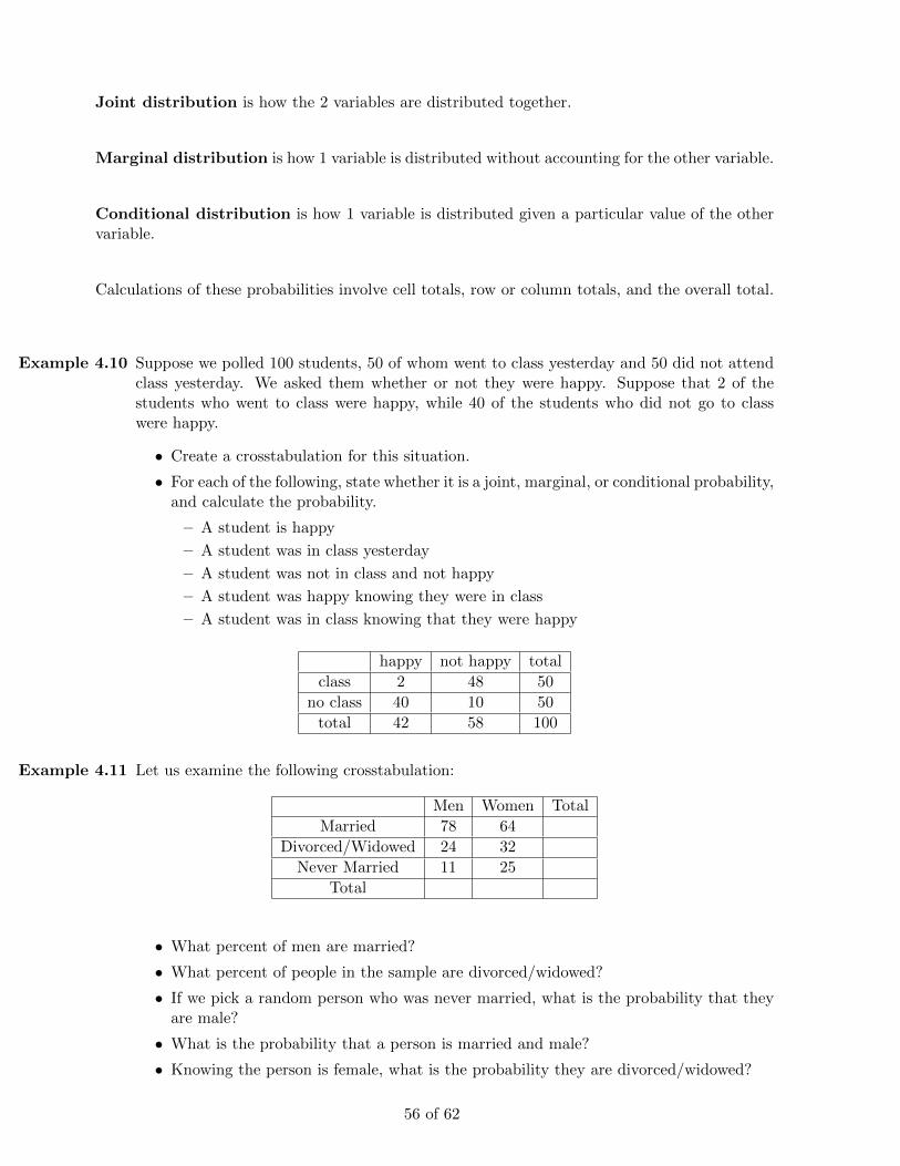
Joint distribution is how the 2 variables are distributed together.

Marginal distribution is how 1 variable is distributed without accounting for the other variable.

Conditional distribution is how 1 variable is distributed given a particular value of the othervariable.

Calculations of these probabilities involve cell totals, row or column totals, and the overall total.

Example 4.10 Suppose we polled 100 students, 50 of whom went to class yesterday and 50 did not attendclass yesterday. We asked them whether or not they were happy. Suppose that 2 of thestudents who went to class were happy, while 40 of the students who did not go to classwere happy.

• Create a crosstabulation for this situation.

• For each of the following, state whether it is a joint, marginal, or conditional probability,and calculate the probability.

– A student is happy

– A student was in class yesterday

– A student was not in class and not happy

– A student was happy knowing they were in class

– A student was in class knowing that they were happy

happy not happy total

class 2 48 50

no class 40 10 50

total 42 58 100

Example 4.11 Let us examine the following crosstabulation:

Men Women Total

Married 78 64

Divorced/Widowed 24 32

Never Married 11 25

Total

• What percent of men are married?

• What percent of people in the sample are divorced/widowed?

• If we pick a random person who was never married, what is the probability that theyare male?

• What is the probability that a person is married and male?

• Knowing the person is female, what is the probability they are divorced/widowed?

56 of 62

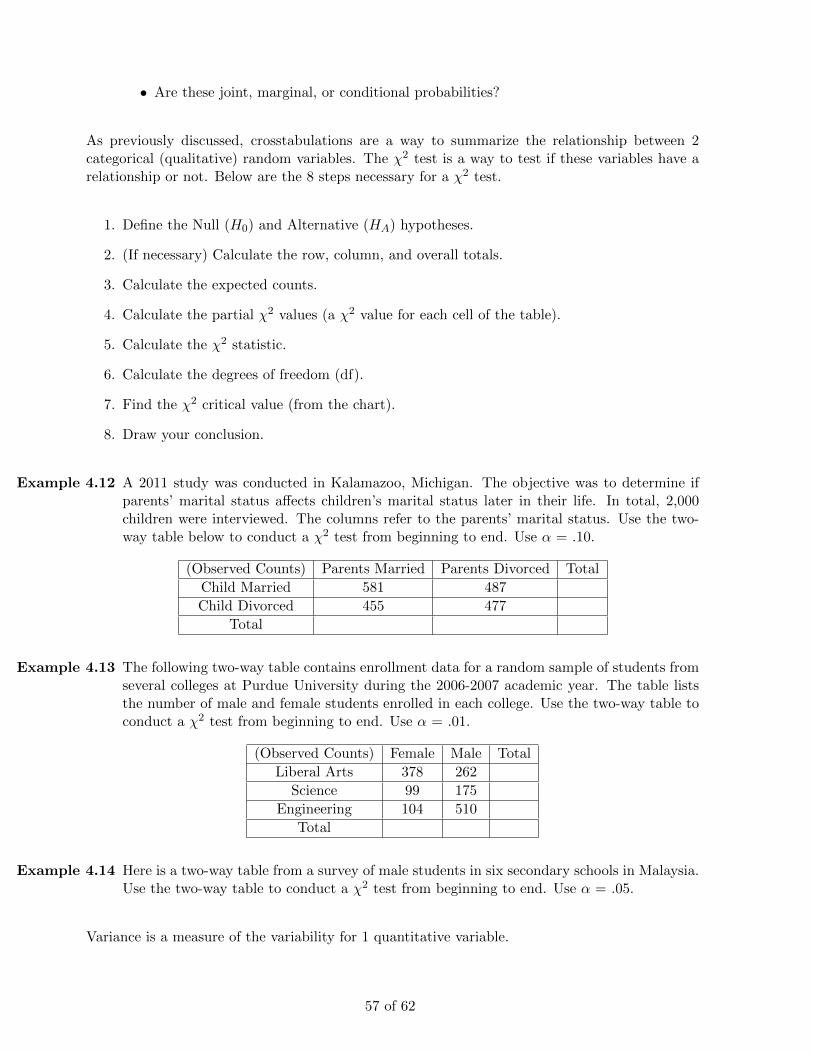
• Are these joint, marginal, or conditional probabilities?

As previously discussed, crosstabulations are a way to summarize the relationship between 2categorical (qualitative) random variables. The χ2 test is a way to test if these variables have arelationship or not. Below are the 8 steps necessary for a χ2 test.

1. Define the Null (H0) and Alternative (HA) hypotheses.

2. (If necessary) Calculate the row, column, and overall totals.

3. Calculate the expected counts.

4. Calculate the partial χ2 values (a χ2 value for each cell of the table).

5. Calculate the χ2 statistic.

6. Calculate the degrees of freedom (df).

7. Find the χ2 critical value (from the chart).

8. Draw your conclusion.

Example 4.12 A 2011 study was conducted in Kalamazoo, Michigan. The objective was to determine ifparents’ marital status affects children’s marital status later in their life. In total, 2,000children were interviewed. The columns refer to the parents’ marital status. Use the two-way table below to conduct a χ2 test from beginning to end. Use α = .10.

(Observed Counts) Parents Married Parents Divorced Total

Child Married 581 487

Child Divorced 455 477

Total

Example 4.13 The following two-way table contains enrollment data for a random sample of students fromseveral colleges at Purdue University during the 2006-2007 academic year. The table liststhe number of male and female students enrolled in each college. Use the two-way table toconduct a χ2 test from beginning to end. Use α = .01.

(Observed Counts) Female Male Total

Liberal Arts 378 262

Science 99 175

Engineering 104 510

Total

Example 4.14 Here is a two-way table from a survey of male students in six secondary schools in Malaysia.Use the two-way table to conduct a χ2 test from beginning to end. Use α = .05.

Variance is a measure of the variability for 1 quantitative variable.

57 of 62

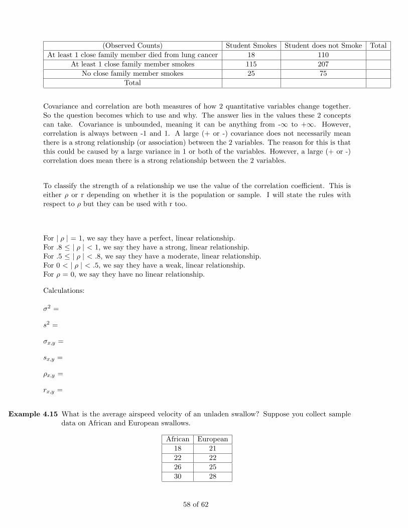
(Observed Counts) Student Smokes Student does not Smoke Total

At least 1 close family member died from lung cancer 18 110

At least 1 close family member smokes 115 207

No close family member smokes 25 75

Total

Covariance and correlation are both measures of how 2 quantitative variables change together.So the question becomes which to use and why. The answer lies in the values these 2 conceptscan take. Covariance is unbounded, meaning it can be anything from -∞ to +∞. However,correlation is always between -1 and 1. A large (+ or -) covariance does not necessarily meanthere is a strong relationship (or association) between the 2 variables. The reason for this is thatthis could be caused by a large variance in 1 or both of the variables. However, a large (+ or -)correlation does mean there is a strong relationship between the 2 variables.

To classify the strength of a relationship we use the value of the correlation coefficient. This iseither ρ or r depending on whether it is the population or sample. I will state the rules withrespect to ρ but they can be used with r too.

For | ρ | = 1, we say they have a perfect, linear relationship.For .8 ≤ | ρ | < 1, we say they have a strong, linear relationship.For .5 ≤ | ρ | < .8, we say they have a moderate, linear relationship.For 0 < | ρ | < .5, we say they have a weak, linear relationship.For ρ = 0, we say they have no linear relationship.

Calculations:

σ2 =

s2 =

σx,y =

sx,y =

ρx,y =

rx,y =

Example 4.15 What is the average airspeed velocity of an unladen swallow? Suppose you collect sampledata on African and European swallows.

African European

18 21

22 22

26 25

30 28

58 of 62

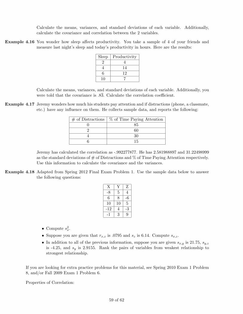
Calculate the means, variances, and standard deviations of each variable. Additionally,calculate the covariance and correlation between the 2 variables.

Example 4.16 You wonder how sleep affects productivity. You take a sample of 4 of your friends andmeasure last night’s sleep and today’s productivity in hours. Here are the results:

Sleep Productivity

2 4

4 14

6 12

10 7

Calculate the means, variances, and standard deviations of each variable. Additionally, youwere told that the covariance is .83. Calculate the correlation coefficient.

Example 4.17 Jeremy wonders how much his students pay attention and if distractions (phone, a classmate,etc.) have any influence on them. He collects sample data, and reports the following:

# of Distractions % of Time Paying Attention

0 85

2 60

4 30

6 15

Jeremy has calculated the correlation as -.992277877. He has 2.581988897 and 31.22498999as the standard deviations of # of Distractions and % of Time Paying Attention respectively.Use this information to calculate the covariance and the variances.

Example 4.18 Adapted from Spring 2012 Final Exam Problem 1. Use the sample data below to answerthe following questions:

X Y Z

-8 5 4

6 8 -6

10 10 5

-12 4 -3

-1 3 9

• Compute s2x.

• Suppose you are given that rx,z is .0795 and sz is 6.14. Compute sx,z.

• In addition to all of the previous information, suppose you are given sx,y is 21.75, sy,zis -4.25, and sy is 2.9155. Rank the pairs of variables from weakest relationship tostrongest relationship.

If you are looking for extra practice problems for this material, see Spring 2010 Exam 1 Problem8, and/or Fall 2009 Exam 1 Problem 6.

Properties of Correlation:

59 of 62

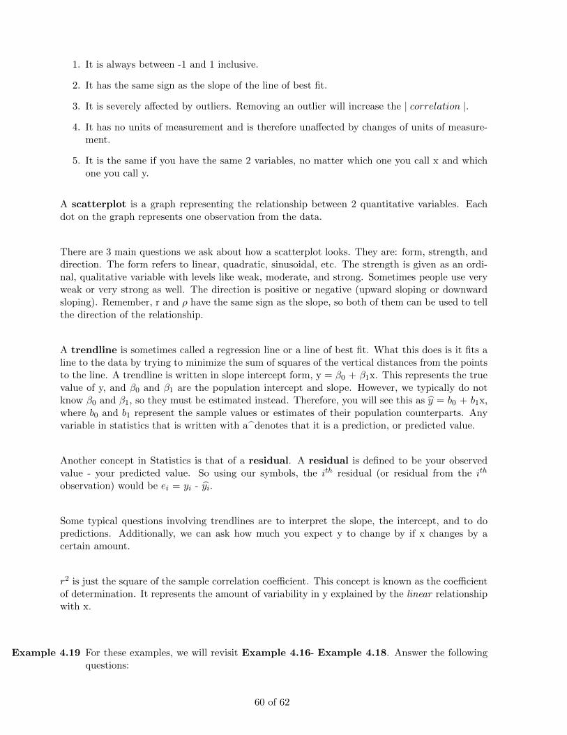
1. It is always between -1 and 1 inclusive.

2. It has the same sign as the slope of the line of best fit.

3. It is severely affected by outliers. Removing an outlier will increase the | correlation |.

4. It has no units of measurement and is therefore unaffected by changes of units of measure-ment.

5. It is the same if you have the same 2 variables, no matter which one you call x and whichone you call y.

A scatterplot is a graph representing the relationship between 2 quantitative variables. Eachdot on the graph represents one observation from the data.

There are 3 main questions we ask about how a scatterplot looks. They are: form, strength, anddirection. The form refers to linear, quadratic, sinusoidal, etc. The strength is given as an ordi-nal, qualitative variable with levels like weak, moderate, and strong. Sometimes people use veryweak or very strong as well. The direction is positive or negative (upward sloping or downwardsloping). Remember, r and ρ have the same sign as the slope, so both of them can be used to tellthe direction of the relationship.

A trendline is sometimes called a regression line or a line of best fit. What this does is it fits aline to the data by trying to minimize the sum of squares of the vertical distances from the pointsto the line. A trendline is written in slope intercept form, y = β0 + β1x. This represents the truevalue of y, and β0 and β1 are the population intercept and slope. However, we typically do notknow β0 and β1, so they must be estimated instead. Therefore, you will see this as y = b0 + b1x,where b0 and b1 represent the sample values or estimates of their population counterparts. Anyvariable in statistics that is written with adenotes that it is a prediction, or predicted value.

Another concept in Statistics is that of a residual. A residual is defined to be your observedvalue - your predicted value. So using our symbols, the ith residual (or residual from the ith

observation) would be ei = yi - yi.

Some typical questions involving trendlines are to interpret the slope, the intercept, and to dopredictions. Additionally, we can ask how much you expect y to change by if x changes by acertain amount.

r2 is just the square of the sample correlation coefficient. This concept is known as the coefficientof determination. It represents the amount of variability in y explained by the linear relationshipwith x.

Example 4.19 For these examples, we will revisit Example 4.16- Example 4.18. Answer the followingquestions:

60 of 62

• Interpret the y-intercept.

• Interpret the slope.

• Interpret the r2 value.

• Calculate the value of r.

• Is a prediction at the value of 4 appropriate? If so, what is the predicted value?

• Is a prediction at the value of 22 appropriate? If so, what is the predicted value?

• If applicable, calculate a residual from your predicted value(s) above. What does thistell you about the position of the observation compared to the regression line?

• If one were to increase x by 2 units, how would you expect y to change?

• If one were to decrease x by 3 units, how would you expect y to change?

Example 4.20 Use the graphs labelled graphs 1-4. You have the following possibilities for r values: -1,-.9696, -.4611, -.0490, 0, .0490, .5737, .9696, and 1. Pick the appropriate values for the 4graphs.

If you are looking for extra practice for values of r, you can go to Fall 2011 Final Exam Problem 2or Spring 2012 Final Exam Problem 4. If you are looking for extra practice with scatterplot andregression questions, you can go to Fall 2011 Final Exam Problem 5 or Spring 2012 Final ExamProblem 3.

61 of 62

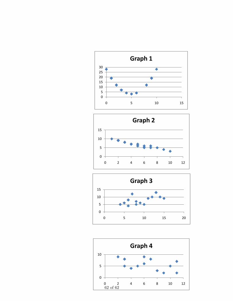
0

5

10

15

20

25

30

0 5 10 15

Graph 1

0

5

10

15

0 2 4 6 8 10 12

Graph 2

0

5

10

15

0 5 10 15 20

Graph 3

0

5

10

0 2 4 6 8 10 12

Graph 4

62 of 62

stat 225: introduction to probability models course ...mrlawlor/student_notes.pdf · stat 225:...

Documents