introduction to mechanics papachristou 2020
TRANSCRIPT
COSTAS J. PAPACHRISTOU
INTRODUCTION TO
MECHANICS
OF PARTICLES AND SYSTEMS

Introduction to
MECHANICS
of Particles and Systems
Costas J. Papachristou
Department of Physical Sciences Hellenic Naval Academy

i
PREFACE
Newtonian Mechanics is, traditionally, the first stage of “initiation” of a college stu-dent into Physics. It is perhaps the only truly autonomous subject area of Physics, in the sense that it can be taught as a self-contained entity without the need for support from other areas of physical science. This textbook is based on lecture notes (origi-nally in Greek) used by this author in his two-semester course of introductory Me-chanics, taught at the Hellenic Naval Academy (the Naval Academy of Greece). It is evident that no serious approach to Mechanics (at least at the university level) is possible without the support of higher Mathematics. Indeed, the central law of Me-chanics, Newton’s Second Law, carries a rich mathematical structure being both a vector equation and a differential equation. An effort is thus made to familiarize the student from the outset with the use of some basic mathematical tools, such as vec-tors, differential operators and differential equations. To this end, the first chapter contains the elements of vector analysis that will be needed in the sequel, while the Mathematical Supplement constitutes a brief introduction to the aforementioned con-cepts of differential calculus. The main text may be subdivided into three parts. In the first part (Chapters 2-5) we study the mechanics of a single particle (and, more generally, of a body that executes purely translational motion) while the second part (Chap. 6-8) introduces to the me-chanics of more complex structures such as systems of particles, rigid bodies and ideal fluids. The third part consists of 60 fully solved problems. I urge the student to try to solve each problem on his/her own before looking at the accompanying solu-tion. Some useful supplementary material may also be found in the Appendices. I am indebted to Aristidis N. Magoulas for helping me with the figures. I also thank the Hellenic Naval Academy for publishing the original, Greek version of the book. And, of course, I express my gratitude and appreciation to my wife, Thalia, for her patience and support while this book was written!
Costas J. Papachristou Piraeus, Greece June 2020

ii
iii
CONTENTS
1. VECTORS
1.1 Basic Notions 1 1.2 Rectangular Components of a Vector 3 1.3 Position Vectors 5 1.4 Scalar (“Dot”) Product of Two Vectors 7 1.5 Vector (“Cross”) Product of Two Vectors 8 2. KINEMATICS
2.1 Rectilinear Motion 11 2.2 Special Types of Rectilinear Motion 13 2.3 Curvilinear Motion in Space 15 2.4 Change of Speed 17 2.5 Motion with Constant Acceleration 18 2.6 Tangential and Normal Components 19 2.7 Circular Motion 24 2.8 Relative Motion 26 3. DYNAMICS OF A PARTICLE
3.1 The Law of Inertia 29 3.2 Momentum, Force, and Newton’s 2nd and 3rd Laws 30 3.3 Force of Gravity 34 3.4 Frictional Forces 35 3.5 Systems with Variable Mass 38 3.6 Tangential and Normal Components of Force 39 3.7 Angular Momentum and Torque 41 3.8 Central Forces 46 4. WORK AND ENERGY
4.1 Introduction 48 4.2 Work of a Force 48 4.3 Kinetic Energy and the Work-Energy Theorem 51 4.4 Potential Energy and Conservative Forces 53 4.5 Conservation of Mechanical Energy 56 4.6 Examples of Conservative Forces 58 4.7 Kinetic Friction as a Non-Conservative Force 62 5. OSCILLATIONS
5.1 Simple Harmonic Motion (SHM) 64 5.2 Force in SHM 66 5.3 Energy Relations 68 5.4 Oscillations of a Mass-Spring System 68 5.5 Oscillation of a Pendulum 72 5.6 Differential Equation of SHM 73
iv
6. SYSTEMS OF PARTICLES
6.1 Center of Mass of a System of Particles 76 6.2 Newton’s Second Law and Conservation of Momentum 77 6.3 Angular Momentum of a System of Particles 80 6.4 Kinetic Energy of a System of Particles 83 6.5 Total Mechanical Energy of a System of Particles 85 6.6 Collisions 87 7. RIGID-BODY MOTION
7.1 Rigid Body 92 7.2 Center of Mass of a Rigid Body 92 7.3 Revolution of a Particle About an Axis 95 7.4 Angular Momentum of a Rigid Body 101 7.5 Rigid-Body Equations of Motion 103 7.6 Moment of Inertia and the Parallel-Axis Theorem 106 7.7 Conservation of Angular Momentum 109 7.8 Equilibrium of a Rigid Body 113 7.9 Kinetic and Total Mechanical Energy 115 7.10 Rolling Bodies 117 7.11 The Role of Static Friction in Rolling 119 7.12 Gyroscopic Motion 120 8. ELEMENTARY FLUID MECHANICS
8.1 Ideal Fluid 123 8.2 Hydrostatic Pressure 123 8.3 Fundamental Equation of Hydrostatics 125 8.4 Units of Pressure 128 8.5 Communicating Vessels 129 8.6 Pascal’s Principle 131 8.7 Archimedes’ Principle 132 8.8 Dynamics of the Submerged Body 134 8.9 Equilibrium of a Floating Body 135 8.10 Fluid Flow 137 8.11 Equation of Continuity 139 8.12 Bernoulli’s Equation 140 8.13 Horizontal Flow 142 APPENDICES
A. Composition of Forces Acting in Space 144 B. Some Theorems on the Center of Mass 150 C. Table of Moments of Inertia 154 D. Principal Axes of Rotation 155 E. Variation of Pressure in the Atmosphere 158 F. Proof of Bernoulli’s Equation 159

v
SOLVED PROBLEMS 161
MATHEMATICAL SUPPLEMENT 226
BASIC INTEGRALS 232
INDEX 233

vi
1
CHAPTER 1
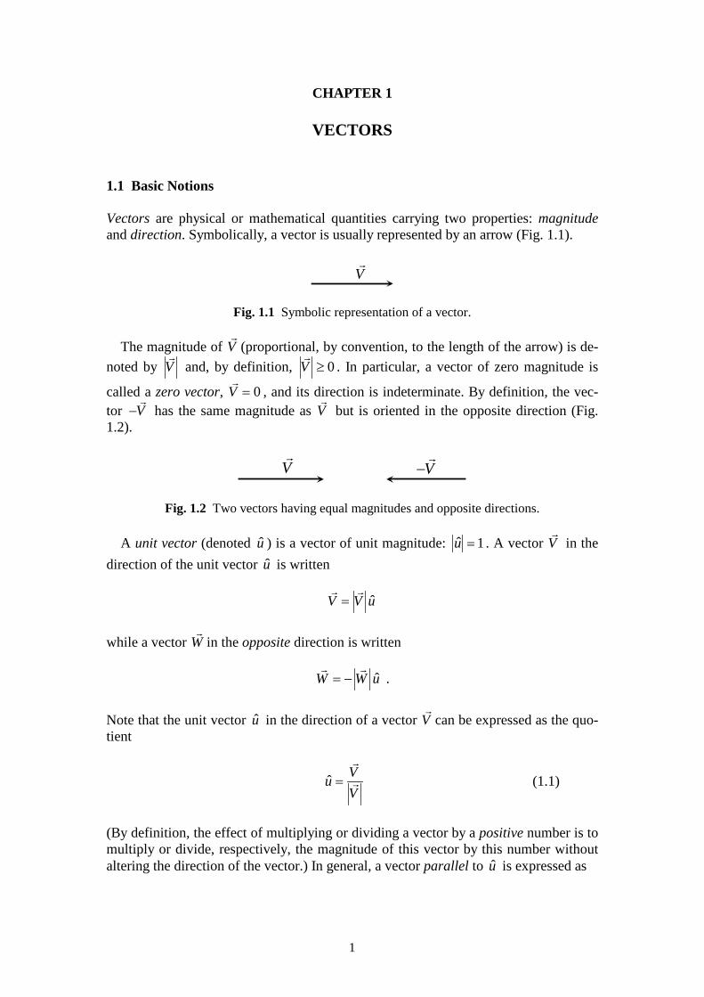
VECTORS 1.1 Basic Notions Vectors are physical or mathematical quantities carrying two properties: magnitude and direction. Symbolically, a vector is usually represented by an arrow (Fig. 1.1).
V�
Fig. 1.1 Symbolic representation of a vector. The magnitude of V
�
(proportional, by convention, to the length of the arrow) is de-
noted by V�
and, by definition, 0V ≥�
. In particular, a vector of zero magnitude is
called a zero vector, 0V =�
, and its direction is indeterminate. By definition, the vec-tor V−
�
has the same magnitude as V�
but is oriented in the opposite direction (Fig. 1.2).
V�
V−�
Fig. 1.2 Two vectors having equal magnitudes and opposite directions. A unit vector (denoted u ) is a vector of unit magnitude: ˆ 1u = . A vector V
�
in the
direction of the unit vector u is written
ˆV V u=� �
while a vector W
�
in the opposite direction is written
ˆW W u= −� �
.
Note that the unit vector u in the direction of a vector V
�
can be expressed as the quo-tient
ˆV
uV
=
�
� (1.1)
(By definition, the effect of multiplying or dividing a vector by a positive number is to multiply or divide, respectively, the magnitude of this vector by this number without altering the direction of the vector.) In general, a vector parallel to u is expressed as
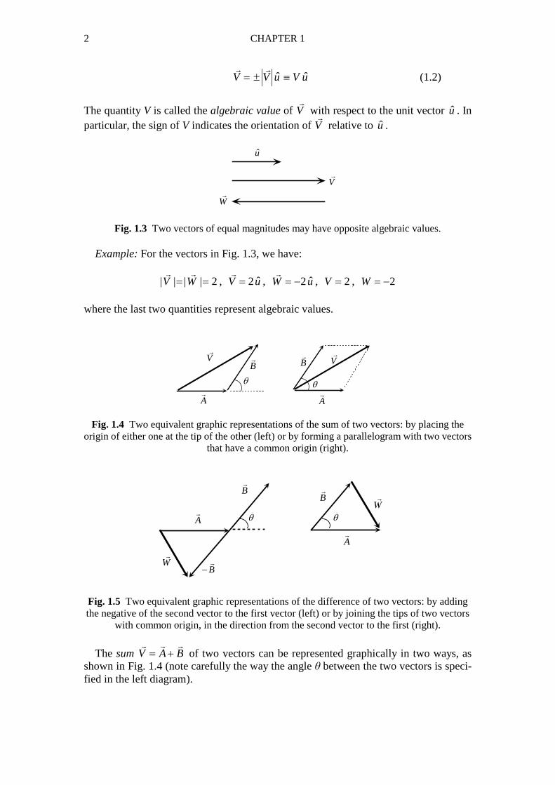
2 CHAPTER 1
A�
B�V
�
θ
A�
B�
V�
θ
A�
B�
B−�W
�
θ θ
A�
B�
W�
ˆ ˆV V u V u= ± ≡� �
(1.2)
The quantity V is called the algebraic value of V
�
with respect to the unit vector u . In particular, the sign of V indicates the orientation of V
�
relative to u .
u
V�
W�
Fig. 1.3 Two vectors of equal magnitudes may have opposite algebraic values. Example: For the vectors in Fig. 1.3, we have:
ˆ ˆ| | | | 2 , 2 , 2 , 2 , 2V W V u W u V W= = = = − = = −� � � �
where the last two quantities represent algebraic values.
Fig. 1.4 Two equivalent graphic representations of the sum of two vectors: by placing the origin of either one at the tip of the other (left) or by forming a parallelogram with two vectors
that have a common origin (right). Fig. 1.5 Two equivalent graphic representations of the difference of two vectors: by adding the negative of the second vector to the first vector (left) or by joining the tips of two vectors
with common origin, in the direction from the second vector to the first (right).
The sum V A B= +�� �
of two vectors can be represented graphically in two ways, as shown in Fig. 1.4 (note carefully the way the angle θ between the two vectors is speci-fied in the left diagram).
VECTORS 3
The difference ( )W A B A B= − ≡ + −� �� � �
of two vectors is found graphically as seen
in Fig. 1.5. In the figure on the right, note that the arrow of A B−� �
is directed toward the tip of A
�
. (Draw the vector B A−��
.) It can be shown (see Exercise 1 at the end of the chapter) that
2 2 1/ 2( 2 cos )A B A B AB θ± = + ±� �
(1.3)
where , ,A A B B= =� �
and where θ is the angle between A�
and B�
.
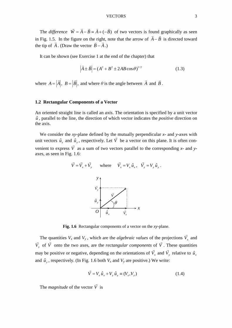
1.2 Rectangular Components of a Vector An oriented straight line is called an axis. The orientation is specified by a unit vector u , parallel to the line, the direction of which vector indicates the positive direction on the axis. We consider the xy-plane defined by the mutually perpendicular x- and y-axes with unit vectors xu and ˆyu , respectively. Let V
�
be a vector on this plane. It is often con-
venient to express V�
as a sum of two vectors parallel to the corresponding x- and y-axes, as seen in Fig. 1.6:
x yV V V= +� � �
where ˆ ˆ,x x x y y yV V u V V u= =� �
.
θ
O ˆxu
ˆ yu
x
y
V�
xV�
yV�
Fig. 1.6 Rectangular components of a vector on the xy-plane. The quantities Vx and Vy , which are the algebraic values of the projections xV
�
and
yV�
of V�
onto the two axes, are the rectangular components of V�
. These quantities
may be positive or negative, depending on the orientations of xV�
and yV�
relative to xu
and ˆyu , respectively. (In Fig. 1.6 both Vx and Vy are positive.) We write:
ˆ ˆ ( , )x x y y x yV V u V u V V= + ≡
�
(1.4)
The magnitude of the vector V�
is
4 CHAPTER 1
2 2x yV V V V≡ = +
�
(1.5)
The angle θ in Fig. 1.6 is measured relative to the positive x semiaxis and it increases counterclockwise. Thus, starting from the x-axis we may form positive or negative angles by moving counterclockwise or clockwise, respectively. We note that
cos , sin , tan yx y
x
VV V V V
Vθ θ θ= = = (1.6)
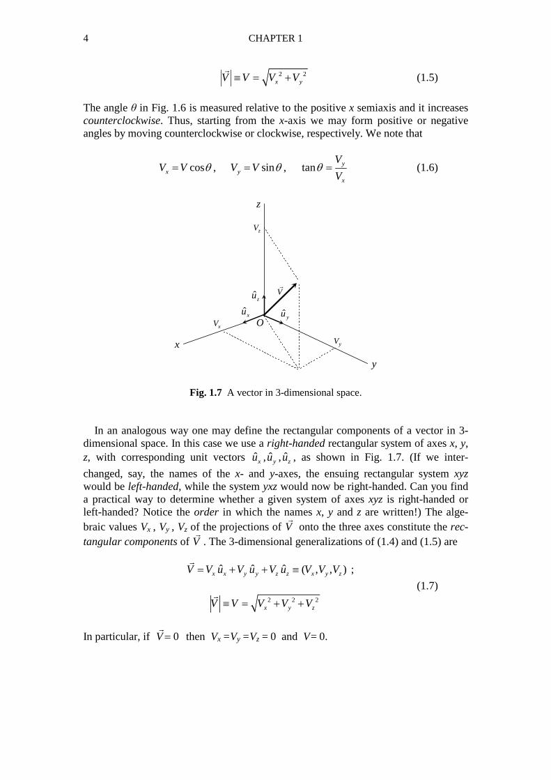
ˆxu ˆ yu
ˆzu
x
y
z
OxV
yV
zV
V�
Fig. 1.7 A vector in 3-dimensional space. In an analogous way one may define the rectangular components of a vector in 3-dimensional space. In this case we use a right-handed rectangular system of axes x, y, z, with corresponding unit vectors ˆ ˆ ˆ, ,x y zu u u , as shown in Fig. 1.7. (If we inter-
changed, say, the names of the x- and y-axes, the ensuing rectangular system xyz would be left-handed, while the system yxz would now be right-handed. Can you find a practical way to determine whether a given system of axes xyz is right-handed or left-handed? Notice the order in which the names x, y and z are written!) The alge-braic values Vx , Vy , Vz of the projections of V
�
onto the three axes constitute the rec-tangular components of V
�
. The 3-dimensional generalizations of (1.4) and (1.5) are ˆ ˆ ˆ ( , , )x x y y z z x y zV V u V u V u V V V= + + ≡
�
;
(1.7)
2 2 2x y zV V V V V≡ = + +
�
In particular, if 0V=�
then Vx =Vy =Vz = 0 and V= 0.
VECTORS 5
Now, assume that ˆ ˆ ˆx x y y z zA A u A u A u= + +�
and ˆ ˆ ˆx x y y z zB B u B u B u= + +�
. Then,
, ,x x y y z zA B A B A B A B= ⇔ = = =� �
(1.8)
Moreover,
ˆ ˆ ˆ( ) ( ) ( )
( , , )x x x y y y z z z
x x y y z z
A B A B u A B u A B u
A B A B A B
± = ± + ± + ±
≡ ± ± ±
� �
(1.9)
In general, the components of a sum of vectors are the sums of the respective compo-nents of the vectors. Thus, let
1 2 ( , , )i x y zi
V V V V V V V= + + ⋅ ⋅ ⋅ ≡ ≡∑� � � �
where ( , , )i ix iy izV V V V≡�
.
Then, , ,x ix y iy z iz
i i i
V V V V V V= = =∑ ∑ ∑ (1.10)
Example: For the vectors (1, 1, 0) , (2,1, 1)A B≡ − ≡ −� �
, we have:
(3,0, 1) , ( 1, 2, 1)A B A B+ ≡ − − ≡ − −� �� �
and
2 2 2 2 23 0 ( 1) 10 , ( 1) ( 2) 1 6A B A B+ = + + − = − = − + − + =� �� �
.
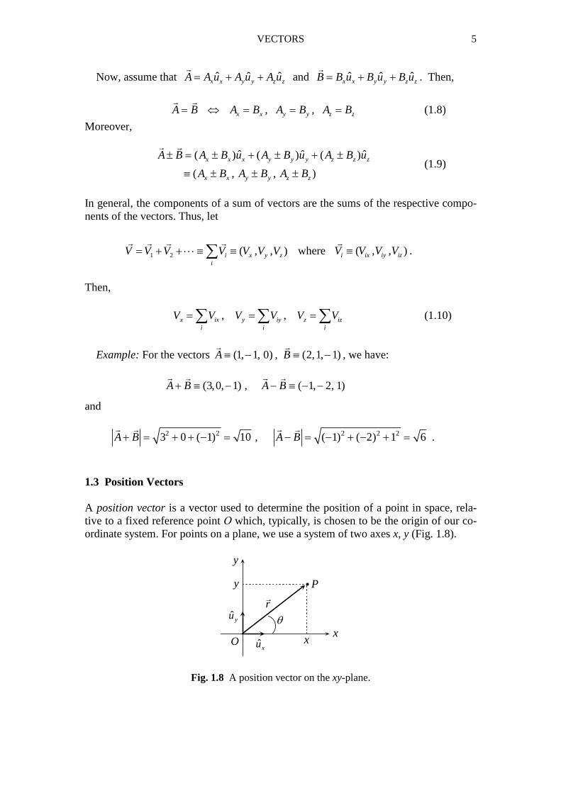
1.3 Position Vectors A position vector is a vector used to determine the position of a point in space, rela-tive to a fixed reference point Ο which, typically, is chosen to be the origin of our co-ordinate system. For points on a plane, we use a system of two axes x, y (Fig. 1.8).
θ
O ˆxu
ˆ yur�
iP
xx
y
y
Fig. 1.8 A position vector on the xy-plane.

6 CHAPTER 1
The vector r OP=����
�
determines the position of point Ρ relative to O. The compo-nents (x, y) of r
�
are the Cartesian coordinates of P. We write: ˆ ˆ ( , )x yr xu yu x y= + ≡
�
(1.11)
Alternatively, we can determine the position of Ρ by using polar coordinates (r, θ), where r r=
�
and where 0 2θ π≤ < or π θ π− < ≤ (by convention, the angle θ in-
creases counterclockwise). We notice that cos , sinx r y rθ θ= = (1.12) or, conversely,
2 2 , tany
r x yx
θ= + = (1.13)
ˆxu ˆ yu
ˆzu
x
y
z
O
r�iP
xy
z
Fig. 1.9 A position vector in 3-dimensional space. For points in space we use a rectangular system of axes x, y, z (Fig. 1.9). We write:
ˆ ˆ ˆ ( , , )x y zr xu yu zu x y z= + + ≡�
;
(1.14) 2 2 2r r x y z= = + +
�
The three quantities (x, y, z) constitute the Cartesian coordinates of point P in space. Alternative systems of coordinates are spherical and cylindrical coordinates, which will not be used in this book (see [1,2]). Now, let P1 , P2 be two points in space with position vectors 1 2,r r
� �
and with coordi-
nates (x1, y1, z1), (x2, y2, z2), respectively (Fig. 1.10). We seek an expression for the distance P1P2 between these points.
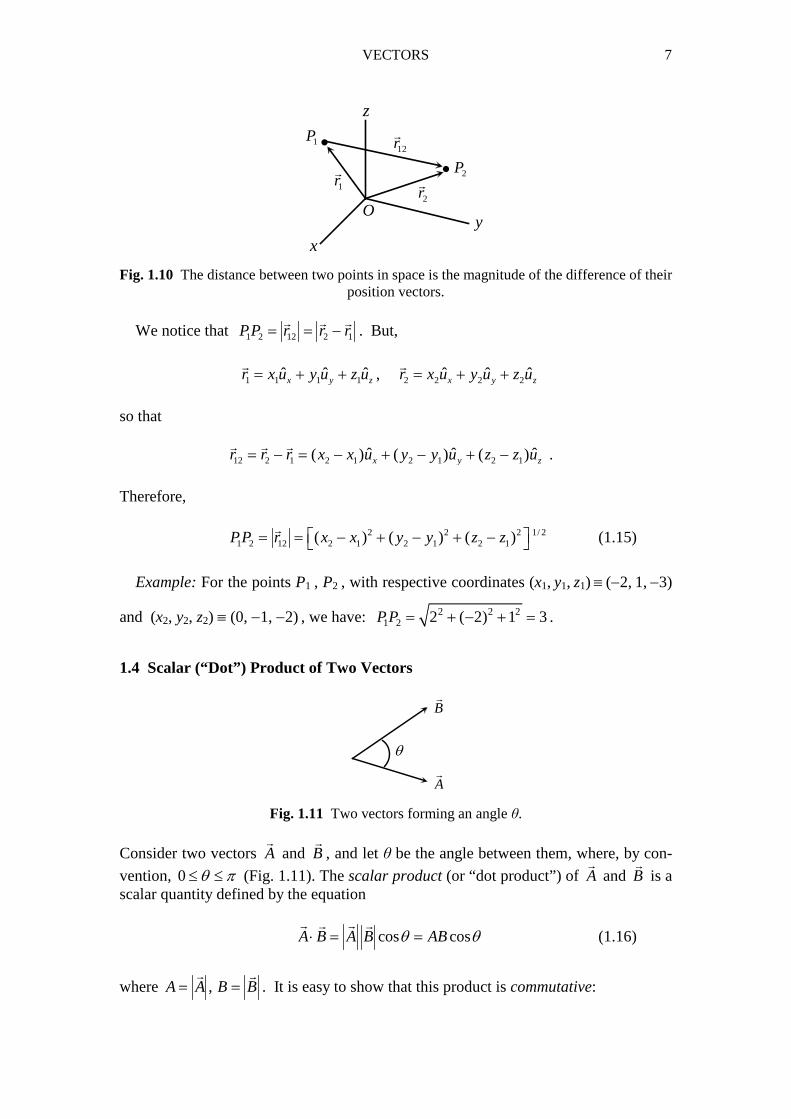
VECTORS 7
Fig. 1.10 The distance between two points in space is the magnitude of the difference of their
position vectors. We notice that 1 2 12 2 1PP r r r= = −
� � �
. But,
1 1 1 1 2 2 2 2ˆ ˆ ˆ ˆ ˆ ˆ,x y z x y zr x u y u z u r x u y u z u= + + = + +
� �
so that 12 2 1 2 1 2 1 2 1ˆ ˆ ˆ( ) ( ) ( )x y zr r r x x u y y u z z u= − = − + − + −
� � �
.
Therefore,
2 2 2 1/ 21 2 12 2 1 2 1 2 1( ) ( ) ( )PP r x x y y z z = = − + − + −
�
(1.15)
Example: For the points P1 , P2 , with respective coordinates (x1, y1, z1) ≡ (−2, 1, −3)
and (x2, y2, z2) ≡ (0, −1, −2) , we have: 2 2 21 2 2 ( 2) 1 3PP = + − + = .
1.4 Scalar (“Dot”) Product of Two Vectors
Fig. 1.11 Two vectors forming an angle θ. Consider two vectors A
�
and B�
, and let θ be the angle between them, where, by con-
vention, 0 θ π≤ ≤ (Fig. 1.11). The scalar product (or “dot product”) of A�
and B�
is a scalar quantity defined by the equation
cos cosA B A B ABθ θ⋅ = =� �� �
(1.16)
where ,A A B B= =� �
. It is easy to show that this product is commutative:
•
•
x
y
z
O
1P
2P1r�
2r�
12r�
A�
B�
θ

8 CHAPTER 1
A B B A⋅ = ⋅� �� �
. In the case where A B=
� �
, we have θ=0, cosθ=1 and
2 2A A A A⋅ = =
� � �
(1.17)
If A�
and B�
are mutually perpendicular, then θ=π/2, cosθ=0 and therefore
0A B A B⋅ = ⇔ ⊥� �� �
(1.18) As can be shown [1],
( ) ( )A B A Bλ λ⋅ = ⋅� �� �
, ( ) ( ) ( )A B A Bκ λ κλ⋅ = ⋅� �� �
(where κ, λ are scalars) and
( )A B C A B A C⋅ + = ⋅ + ⋅� � � � �� �
. For the unit vectors we can show that ˆ ˆ ˆ ˆ ˆ ˆ ˆ ˆ ˆ ˆ ˆ1 , 0 .x x y y z z x y x z y zu u u u u u u u u u u u⋅ = ⋅ = ⋅ = ⋅ = ⋅ = ⋅ =
Thus, if ˆ ˆ ˆx x y y z zA A u A u A u= + +�
and ˆ ˆ ˆx x y y z zB B u B u B u= + +�
, we find a useful relation
for the dot product in terms of components:
x x y y z zA B A B A B A B⋅ = + +� �
(1.19)
For two equal vectors we are thus led back to (1.17):
22 2 2
x y zA A A A A A⋅ = + + =� � �
(1.20)
1.5 Vector (“Cross”) Product of Two Vectors
i
A�
B�
θ
A B� �
B A��
Fig. 1.12 The two possible orientations of the vector product of two vectors, depending on
the order in which these vectors appear in the product.
VECTORS 9
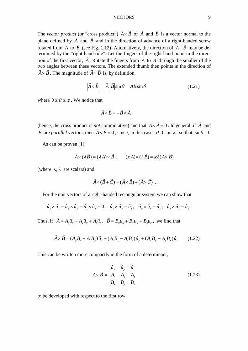
The vector product (or “cross product”) A B×� �
of A�
and B�
is a vector normal to the plane defined by A
�
and B�
and in the direction of advance of a right-handed screw rotated from A
�
to B�
(see Fig. 1.12). Alternatively, the direction of A B� �
may be de-termined by the “right-hand rule”: Let the fingers of the right hand point in the direc-tion of the first vector, A
�
. Rotate the fingers from A�
to B�
through the smaller of the two angles between these vectors. The extended thumb then points in the direction of A B� �
. The magnitude of A B� �
is, by definition,
sin sinA B A B ABθ θ× = =� �� �
(1.21)
where 0 θ π≤ ≤ . We notice that
A B B A× = − ×� �� �
(hence, the cross product is not commutative) and that 0A A× =� �
. In general, if A�
and
B�
are parallel vectors, then 0A B× =� �
, since, in this case, θ=0 or π, so that sinθ=0. As can be proven [1],
( ) ( )A B A Bλ λ× = ×� �� �
, ( ) ( ) ( )A B A Bκ λ κλ× = ×� �� �
(where κ, λ are scalars) and
( ) ( ) ( )A B C A B A C× + = × + ×� � � � �� �
. For the unit vectors of a right-handed rectangular system we can show that ˆ ˆ ˆ ˆ ˆ ˆ ˆ ˆ ˆ ˆ ˆ ˆ ˆ ˆ ˆ0, , ,x x y y z z x y z y z x z x yu u u u u u u u u u u u u u u× = × = × = × = × = × = .
Thus, if ˆ ˆ ˆ ˆ ˆ ˆ,x x y y z z x x y y z zA A u A u A u B B u B u B u= + + = + +� �
, we find that
ˆ ˆ ˆ( ) ( ) ( )y z z y x z x x z y x y y x zA B A B A B u A B A B u A B A B u× = − + − + −� �
(1.22)
This can be written more compactly in the form of a determinant,
ˆ ˆ ˆx y z
x y z
x y z
u u u
A B A A A
B B B
× =� �
(1.23)
to be developed with respect to the first row.
10 CHAPTER 1
Exercises
1. Consider the vectors ( , , )x y zA A A A≡�
and ( , , )x y zB B B B≡�
, and let θ be the angle
between them. By using the properties of the scalar product, show the following:
a. ( )1/ 22 2
2 cosA B A B A B θ± = + ±� � �� � �
b. ( ) ( )1/ 2 1/ 22 2 2 2 2 2
cos x x y y z z
x y z x y z
A B A B A B
A A A B B Bθ
+ +=
+ + + +
c. If A B⊥� �
, then 2 2 2 2
A B A B A B+ = − = +� � �� � �
(Pythagorean theorem)
2. Let ( , , ),x y zA A A A≡�
( , , )x y zB B B B≡�
, ( , , )x y zC C C C≡�
.
a. Show that
( )x y z
x y z
x y z
A A A
A B C B B B
C C C
⋅ × =� ��
b. By using the properties of determinants, show that
( ) ( ) ( )
( ) 0
A B C B C A C A B
A A B
⋅ × = ⋅ × = ⋅ ×
⋅ × =
� � � � � �� � �
� � �
3. Find the value of α in order that the vectors 1 3
, ,2 2
A α ≡
�
and ( 3,3, 1)B ≡ − −�
be
mutually perpendicular.
4. Find the values of α and β in order that the vectors (1, ,3)A α≡�
and
( 2, 4, )B β≡ − −�
be parallel to each other.
References
1. A.I. Borisenko, I.E. Tarapov, Vector and Tensor Analysis with Applications (Dover, 1979)
2. M.D. Greenberg, Advanced Engineering Mathematics, 2nd Edition (Prentice-Hall, 1998)
11
CHAPTER 2
KINEMATICS 2.1 Rectilinear Motion Kinematics is the branch of Mechanics that studies motion per se, regardless of the physical factors that cause or affect it. (The connection between cause and effect is the subject of Dynamics, to be discussed in the next chapter.) The simplest type of motion is rectilinear motion, i.e., motion along a straight line. Such a line could be, e.g., the x-axis on which we have defined a positive orientation in the direction of the unit vector ˆxu , as well as a point O (an origin) at which x=0
(Fig. 2.1).
• •0x=
O ˆxu r�
x
Ax
Fig. 2.1 Motion along the x-axis; the value of x determines the momentary position A of the
moving object. The position A of the moving object, at time t, is specified by the position vector
ˆxOA r xu= =����
�
where x and r
�
are functions of t : ( ) , ( )x x t r r t= =� �
. We note that x>0 or x<0, de-pending on whether the object is on the right or on the left of O, respectively. The velocity of the object at point Α, at time t, is defined as the time derivative of the position vector; i.e., it is the vector
ˆ ˆ( )x x
dr d dxv xu u
dt dt dt= = =�
�
(where we have taken into account that ˆxu is constant). We write:
ˆxv vu=�
where dx
v vdt
= = ±�
(2.1)
In the above relation, v is the algebraic value of the velocity with respect to the unit vector ˆxu . The magnitude of the velocity, equal to |v|, is called the speed. In general, v
and v�
are functions of t. The sign of v indicates the instantaneous direction of motion: if v>0, the object is moving in the positive direction of the x-axis (i.e., to the right, as seen in Fig. 2.1), while if v<0, the object is moving in the negative direction (to the left). In S.I. units, v is expressed in m/s=m.s –1.
12 CHAPTER 2
Given the function v=v(t), we can find the position x(t) of the object at all times t by integrating (cf. Mathematical Supplement). From (2.1) we have:
dxv dx vdt
dt= ⇒ = .
We integrate the above differential equation, making the additional assumption (initial condition) that, at the moment t=t0 , the instantaneous position of the object is x=x0 :
0 0 00
x t t
x t tdx vdt x x vdt= ⇒ − = ⇒∫ ∫ ∫
0
0
t
tx x vdt= + ∫ (2.2)
The difference x−x0 is called the displacement of the object from point x0 . The acceleration of the object at time t is the derivative of the velocity vector:
ˆ ˆ( )x x
dv d dva vu u
dt dt dt= = =�
�
.
We write:
ˆxa au=�
where 2
2
dv d xa a
dt dt= = = ±
�
(2.3)
The unit of acceleration in the S.I. system is m/s2=m.s –2 . The quantity a in (2.3) represents the algebraic value of the acceleration. For a given function a=a(t), and by assuming that at the moment t=t0 the moving object has a velocity v=v0, we find the velocity v(t) at all times t by integrating:
0 0
v t
v t
dva dv adt dv adt
dt= ⇒ = ⇒ = ⇒∫ ∫
0
0
t
tv v adt= + ∫ (2.4)
If we know the acceleration as a function of x, a=a(x), we can find the velocity as a function of position, as follows: By dividing the relations dv=adt and dx=vdt in order to eliminate t, we get: vdv=adx. We now integrate this relation, assuming that v=v0 at the position x=x0 :
0 0 0
2 20
2 2
v x x
v x x
v vvdv adx adx= ⇒ − = ⇒∫ ∫ ∫
0
2 20 2
x
xv v adx= + ∫ (2.5)

KINEMATICS 13
Two observations are in order regarding equation (2.5): 1. In order for (2.5) to make sense physically, the right-hand side must be nonnega-tive. This may place restrictions on the admissible values of x, which means that the object may not be allowed to move on the entire x-axis. 2. To find v itself (rather than just its absolute value) from relation (2.5), we must take the square root of the right-hand side (the latter assumed nonnegative). This process will yield two values for v, with opposite signs. One of these values must be excluded, however, since its sign will not be consistent with that of v0 . Note also that, in relations (2.2) and (2.4), the x and v are functions of the variable t that appears on the upper limits of the corresponding integrals. Similarly, in relation (2.5) the quantity v2 is a function of the variable x that appears on the upper limit of the integral. In general, an integral with variable upper limit is a function of that limit [1,2]. 2.2 Special Types of Rectilinear Motion We now apply the general results of the previous section to two familiar cases of rectilinear motion. 1. Uniform rectilinear motion: v=constant, a=0 This is the motion with constant velocity (in magnitude and direction). Relation (2.2) yields (by putting t0=0):
0 00 0
t tx x vdt x v dt= + = + ⇒∫ ∫
0x x vt= + (2.6)
2. Uniformly accelerated rectilinear motion: a=constant ≠ 0 By relations (2.4) and (2.2) we find (putting t0=0):
0 00 0
t tv v adt v a dt= + = + ⇒∫ ∫
0v v at= + (2.7)
0 0 0 0 00 0 0 0( )
t t t tx x vdt x v at dt x v dt a tdt= + = + + = + + ⇒∫ ∫ ∫ ∫
20 0
1
2x x v t at= + + (2.8)
14 CHAPTER 2
i 0O x=
x
ˆxu
0v�
0v>
0v<
a�
Furthermore, relation (2.5) gives:
0 0
2 2 20 02 2
x x
x xv v adx v a dx= + = + ⇒∫ ∫
2 20 02 ( )v v a x x= + − (2.9)
Note that the same result is found by eliminating t between (2.7) and (2.8). Note also that, since the right-hand side of (2.9) must be nonnegative, the acceptable values of x may be restricted; this, in turn, will place a restriction on the possible positions of the moving object. Example: Projectile motion
Fig. 2.2 Projectile motion along the vertical x-axis. At time t0=0, a bullet is fired straight upward from a point Ο (at which x0=0) of the vertical x-axis, with initial velocity 0 0 0ˆ ( 0)xv v u v= >
�
(Fig. 2.2). We assume that the
bullet is subject only to the force of gravity (we ignore air resistance). Thus, the accel-eration of the projectile equals the acceleration of gravity, which is always directed downward, regardless of the direction of motion (upward or downward) of the projec-tile. In vector form,
ˆ ˆx xa g u au a g= − ≡ ⇒ = −�
where g is approximately equal to 9.8 m/s2. We notice that a is constant, and therefore the motion is uniformly accelerated. The equations of motion are:
0 0
2 20 0 0
2 2 20 0 0
,
1 1,
2 22 ( ) 2 .
v v at v gt
x x v t at v t gt
v v a x x v gx
= + = −
= + + = −
= + − = −
The projectile will reach a maximum height x=h, where it will stop momentarily at time t=th ; it will then start moving downward, toward the point of ejection O. To find h and th , we use the first two equations of motion:
KINEMATICS 15
00
22 0
0
0 ;
1.
2 2
h h h
h h
vv v gt t
g
vh v t gt
g
= − = ⇒ =
= − =
The maximum height h may also be determined by noting that, in order for the right-hand side of the third equation of motion to be nonnegative, the value of x must not exceed v0
2/2g. Note also that v>0 for 0< t < th , while v<0 for t > th . What is the physical meaning of this? (Notice that we chose the positive direction of the x-axis upward.) Exercise: Find the moment at which the bullet returns to Ο, as well as the velocity of return. What do you observe? Also, show that, in a free fall from height h, a body acquires a speed
2v gh= .
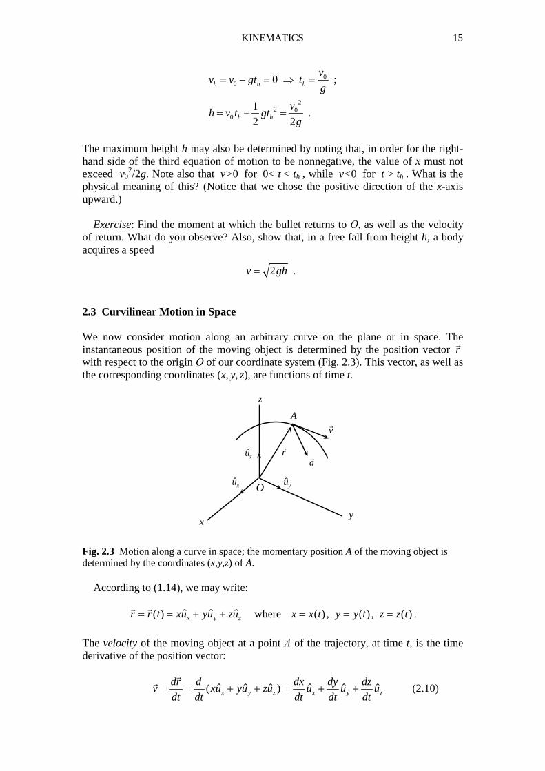
2.3 Curvilinear Motion in Space We now consider motion along an arbitrary curve on the plane or in space. The instantaneous position of the moving object is determined by the position vector r
�
with respect to the origin Ο of our coordinate system (Fig. 2.3). This vector, as well as the corresponding coordinates (x, y, z), are functions of time t. Fig. 2.3 Motion along a curve in space; the momentary position A of the moving object is determined by the coordinates (x,y,z) of A. According to (1.14), we may write:
ˆ ˆ ˆ( ) x y zr r t xu yu zu= = + +� �
where ( ) , ( ) , ( )x x t y y t z z t= = = .
The velocity of the moving object at a point Α of the trajectory, at time t, is the time derivative of the position vector:
ˆ ˆ ˆ ˆ ˆ ˆ( )x y z x y z
dr d dx dy dzv xu yu zu u u u
dt dt dt dt dt= = + + = + +�
�
(2.10)
i
xy
z
ˆxu ˆyu
ˆzu r�
A
a�
v�
O
16 CHAPTER 2
We write:
ˆ ˆ ˆ
, ,
x x y y z z
x y z
v v u v u v u
dx dy dzv v v
dt dt dt
= + +
= = =
�
(2.10)
As will be shown analytically in Sec. 2.6, the velocity vector v
�
is tangent to the tra-jectory at all points and its direction is that of the direction of motion. The magnitude of the velocity, called speed, is
2 2 2x y zv v v v= + +
�
(2.11)
The acceleration of the object at a point Α, at time t, is the time derivative of the velocity:
ˆ ˆ ˆyx zx y z
dvdv dv dva u u u
dt dt dt dt= = + +�
�
(2.12)
We write:
ˆ ˆ ˆ
, ,
x x y y z z
yx zx y z
a a u a u a u
dvdv dva a a
dt dt dt
= + +
= = =
�
(2.12)
As will be shown in Sec. 2.6, the direction of the acceleration vector a
�
is toward the concave (“inner”) side of the trajectory. The magnitude of the acceleration is
2 2 2x y za a a a= + +
�
(2.13)
Example: Assume that the coordinates of a moving particle are given as functions of time by the equations {x=A cos ωt , y=A sin ωt , z=λt}, where Α, ω, λ are positive constants. (What can you say about the trajectory of the particle?) By using (2.10΄) and (2.12) we find the components of velocity and acceleration, respectively, of the particle:
(vx , vy , vz ) ≡ (−ωΑ sin ωt , ωΑ cos ωt , λ) ,
(ax , ay , az ) ≡ (−ω2Α cos ωt , −ω
2Α sin ωt , 0) .
The magnitudes v and a of the corresponding vectors are given by (2.11) and (2.13):
2 2 2 2,v A a Aω λ ω= + = . Note that the speed v of the particle is constant in time, as well as that the vectors of velocity and acceleration are mutually perpendicular [show this by using relations (1.18) and (1.19)]. As will be seen below, these two facts are closely related.
KINEMATICS 17
2.4 Change of Speed Generally speaking, a motion is accelerated if 0a ≠
�
, so that the vector v�
of the ve-locity changes with time. The term “accelerated”, however, is often used with a dif-ferent meaning in Kinematics, a fact that, if not properly pointed out, may lead to con-fusion. Thus, a (generally curvilinear) motion is said to be “accelerated” or “retarded” during a time interval if the speed v v=
�
increases or decreases, respec-
tively, in that interval. If the speed is constant, the motion is called uniform. The kind of motion depends on the angle θ between the vector v
�
of the velocity and the vector a
�
of the acceleration, where, by convention, 0θ π≤ ≤ . In general, cos cosv a v a v aθ θ⋅ = =
� � � �
(2.14)
where a a=
�
. On the other hand,
2 2( ) ( )
2( ) 2 ( ) 2dv dv dv d d v d v dv dv
v a v v v v v vdt dt dt dt dt dv dt dt
⋅ = ⋅ = ⋅ + ⋅ = ⋅ = = = ⇒
� � �
� � � � � � �
dv dv
v a v vdt dt
⋅ = ⋅ =�
� � �
(2.15)
where we have used (1.17), and where it should be noted carefully that
d vdv dvv v v
dt dt dt≡ ≠
� �
� �
!
By comparing (2.14) and (2.15), we find that
cosdv
adt
θ= (2.16)
Given that 0a > , we note the following:
a. If 02
πθ≤ < then 0
dv
dt> ; v increases and the motion is accelerated.
b. If 2
πθ π< ≤ then 0
dv
dt< ; v decreases and the motion is retarded.
c. If 2
πθ = (that is, if a v⊥
� �
) then 0dv
dt= ; v is constant and the motion is uniform.
Of special importance is the following conclusion:
If the acceleration is perpendicular to the velocity, the speed of the moving ob-ject is constant in time, even though the direction of the velocity is changing. Thus, the motion is uniform.
18 CHAPTER 2
In the case of rectilinear motion, the angle θ between v�
and a�
can only assume two values. If v
�
and a�
are in the same direction, then θ=0 and the motion is acceler-ated, while if v
�
and a�
are in opposite directions, then θ=π and the motion is re-tarded. Now, v
�
and a�
are in the same direction or in opposite directions if 0v a⋅ >� �
or 0v a⋅ <� �
, respectively. Given that ˆxv vu=�
and ˆxa au=�
[see Eqs. (2.1) and (2.3)],
where here v and a are algebraic values ( ,v v a a= ± = ±� �
), we have: v a v a⋅ =� �
.
We thus conclude that
a rectilinear motion is accelerated or retarded, depending on whether the product of the algebraic values of the velocity and the acceleration is positive (va>0) or negative (va<0), respectively.
2.5 Motion with Constant Acceleration We now consider the case where the acceleration a
�
of the moving object is constant in magnitude and direction. We assume that at time t=0 the instantaneous position vector of the object, relative to our coordinate system, is 0r r=
� �
, while the object has
initial velocity 0v v=� �
. We seek ( )r t�
and ( )v t�
for every t >0.
Taking into account that a
�
is a constant vector, we have:
000
v t
v
dva dv adt dv a dt v v at
dt= ⇒ = ⇒ = ⇒ − = ⇒∫ ∫
�
�
�
� � � � � � � �
0v v a t= +
� � �
(2.17)
00 0 0 0 0
r t t
r
drv v at dr v dt atdt dr v dt a tdt
dt= = + ⇒ = + ⇒ = + ⇒∫ ∫ ∫
�
�
�
� � � � � � � � �
20 0
1
2r r v t a t= + +� � � �
(2.18)
We write:
2
0 0 2
tr r r t v a∆ = − = +� � � � �
.
This vector relation is of the form 0r v aκ λ∆ = +
� � �
, with constant 0v�
, a�
and variable
κ, λ. According to Analytic Geometry, the vector 0r r r∆ = −� � �
lies on the constant
plane defined by 0v�
and a�
and passing through the point 0r�
(initial position of the
moving object). On the same plane will therefore always lie the tip of the position vector r
�
of the object. We conclude that
KINEMATICS 19
motion with constant acceleration (in magnitude and direction) takes place on a constant plane.1
An example is motion of a body in the gravitational field near the surface of the Earth, in a relatively small region of space where this field may be considered uni-form. If we ignore air resistance, the body is subject to the constant acceleration of gravity g
�
(directed downward, toward the surface of the Earth) and its path is con-
fined to the plane defined by the body’s initial velocity 0v�
and the acceleration g�
(the
plane of motion is perpendicular to the surface of the Earth). 2.6 Tangential and Normal Components The velocity v
�
and the acceleration a�
of a moving object are vectors of absolute physical and geometrical substance, independent of the choice of a system of axes (x, y, z) in our space. If we choose a different set of axes (x΄, y΄, z ), with different ori-gin and orientation relative to (x, y, z), the components of v
�
and a�
will change but the vectors themselves, as geometrical quantities, will remain the same. We will now in-troduce a system of components that is associated with the trajectory itself of the moving object.
ii
r�
r ′�
A
A′
O
C r∆�
s s∆+
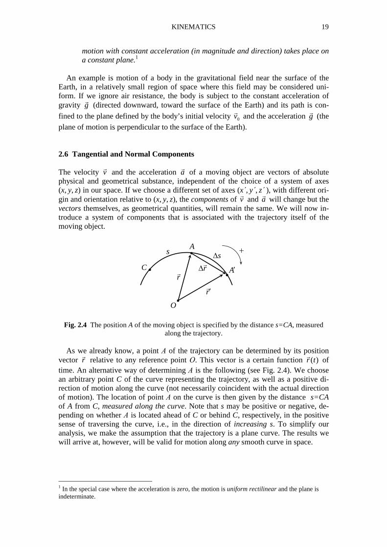
Fig. 2.4 The position A of the moving object is specified by the distance s=CA, measured along the trajectory.
As we already know, a point Α of the trajectory can be determined by its position vector r
�
relative to any reference point Ο. This vector is a certain function ( )r t�
of time. An alternative way of determining Α is the following (see Fig. 2.4). We choose an arbitrary point C of the curve representing the trajectory, as well as a positive di-rection of motion along the curve (not necessarily coincident with the actual direction of motion). The location of point Α on the curve is then given by the distance s=CA of A from C, measured along the curve. Note that s may be positive or negative, de-pending on whether Α is located ahead of C or behind C, respectively, in the positive sense of traversing the curve, i.e., in the direction of increasing s. To simplify our analysis, we make the assumption that the trajectory is a plane curve. The results we will arrive at, however, will be valid for motion along any smooth curve in space.
1 In the special case where the acceleration is zero, the motion is uniform rectilinear and the plane is indeterminate.
20 CHAPTER 2
We consider the points Α and Α΄ of the trajectory, through which points the object passes at times t and t΄, respectively. Let r
�
and r΄�
be the position vectors of Α and Α΄ relative to Ο. We call r r ΄ r∆ = −
� � �
and ∆t = t΄–t, and we write:
( ) , ( ) ( ) ( )r r t r ΄ r t΄ r t t r t r= = = + ∆ = + ∆� � � � � � �
. The velocity at point Α, at time t, is
0 0
( ) ( )lim limt t
dr r t t r t rv
dt t t∆ → ∆ →
+ ∆ − ∆= = =
∆ ∆
� � � �
�
.
But, r r s
t s t
∆ ∆ ∆=
∆ ∆ ∆
� �
, so that
0 0 0lim lim limt s t
r r s
t s t∆ → ∆ → ∆ →
∆ ∆ ∆ = ∆ ∆ ∆
� �
(since ∆s → 0 when ∆t → 0). We thus have:
dr dr ds
vdt ds dt
= =� �
�
(2.19)
This relation expresses the derivative of a composite function, given that ( )r r s=
� �
and s=s(t), so that ( )r r t=
� �
. We now seek the geometrical significance of the vector /dr ds
�
. We notice that this
vector is the limit of /r s∆ ∆�
for ∆s→0. As ∆s→0, the vector /r s∆ ∆�
tends to become tangent to the trajectory at point Α, while its direction is that of increasing s (∆s>0); that is, it points toward the positive direction of traversing the curve. Moreover,
/ 1r s∆ ∆ →�
as ∆s→0. We conclude that /dr ds�
is a unit vector tangent to the trajec-
tory at Α and oriented in the positive direction of motion on the path. We write:
ˆT
dru
ds=�
(2.20)
Relation (2.19) now takes on the form
ˆ ˆT T
dsv u vu
dt= =�
(2.21)
where v is the algebraic value of the velocity with respect to the unit vector ˆTu :
ds
v vdt
= = ±�
.
Thus, if v>0 the motion is in the positive direction (increasing s), while if v<0 the motion is in the negative direction (decreasing s). Note that the unit vector Tu is
KINEMATICS 21
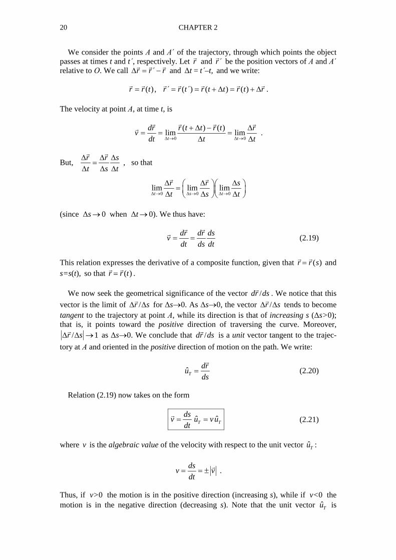
always in the positive direction, regardless of the direction of motion! (In Fig. 2.5 the motion is in the positive direction; thus v>0.) As seen from (2.21), the velocity is a vector tangent to the trajectory.
ˆTuv�
A
+
Fig. 2.5 The velocity is a vector tangent to the trajectory at each point of the latter.
Our study of acceleration begins with an important remark:
1. A component of acceleration parallel to the velocity may alter the magnitude but not the direction of the velocity. (This is the case in accelerated rectilinear motion.)
2. A component of acceleration normal to the velocity may change the direction but not the magnitude of the velocity. (This is a direct consequence of the dis-cussion in Sec. 2.4.)
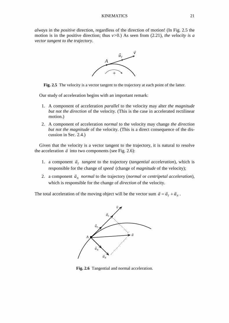
Given that the velocity is a vector tangent to the trajectory, it is natural to resolve the acceleration a
�
into two components (see Fig. 2.6):
1. a component Ta�
tangent to the trajectory (tangential acceleration), which is
responsible for the change of speed (change of magnitude of the velocity);
2. a component Na�
normal to the trajectory (normal or centripetal acceleration),
which is responsible for the change of direction of the velocity. The total acceleration of the moving object will be the vector sum T Na a a= +
� � �
.
A
ˆNu
Na�
a�
ˆTu
Ta�
v�
Fig. 2.6 Tangential and normal acceleration.
22 CHAPTER 2
To evaluate Ta�
and Na�
we differentiate (2.21) with respect to t :
ˆ
ˆ ˆ( ) TT T
dv d dv dua vu u v
dt dt dt dt= = = +�
�
(2.22)
The vector ˆTdu
dt is normal to ˆTu . Indeed,
2ˆ 1 1
ˆ ˆ ˆ ˆ( ) ( ) 02 2
TT T T T
du d du u u u
dt dt dt⋅ = ⋅ = = ,
given that ˆ 1Tu = = constant. Moreover, ˆTdu
dt is directed toward the concave (“inner”)
side of the trajectory, since this is the case with the infinitesimal change ˆTdu of ˆTu .
[By (2.22), then, the acceleration a�
of the moving object is oriented toward the concavity of the curve.] We thus consider a unit vector ˆNu normal to the trajectory
and directed “inward”, and we write:
ˆˆ ˆ
ˆ ˆTT TN N
dudu duu u
dt dt dt= = (2.23)
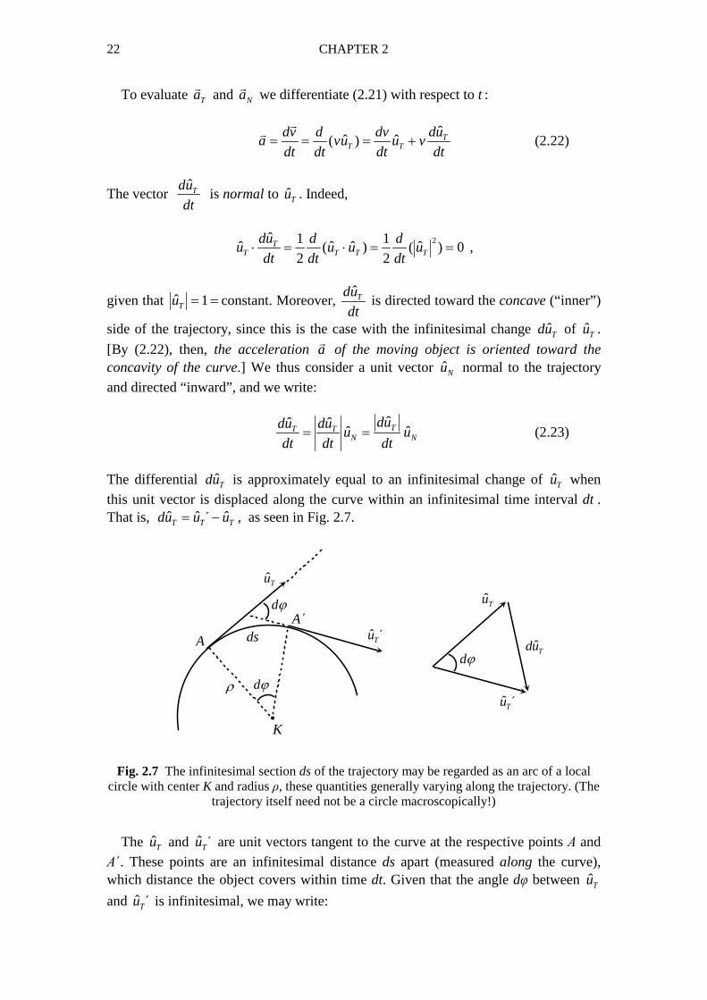
The differential ˆTdu is approximately equal to an infinitesimal change of ˆTu when
this unit vector is displaced along the curve within an infinitesimal time interval dt . That is, ˆ ˆ ˆT T Tdu u΄ u= − , as seen in Fig. 2.7.
A
A΄ds
dϕ
dϕ
dϕ
ρ
K
ˆTu
ˆTu
ˆTu ΄
ˆTu ΄
ˆTdu
i
Fig. 2.7 The infinitesimal section ds of the trajectory may be regarded as an arc of a local circle with center K and radius ρ, these quantities generally varying along the trajectory. (The
trajectory itself need not be a circle macroscopically!)
The ˆTu and ˆTu ΄ are unit vectors tangent to the curve at the respective points Α and
Α΄. These points are an infinitesimal distance ds apart (measured along the curve), which distance the object covers within time dt. Given that the angle dφ between Tu
and ˆTu ΄ is infinitesimal, we may write:
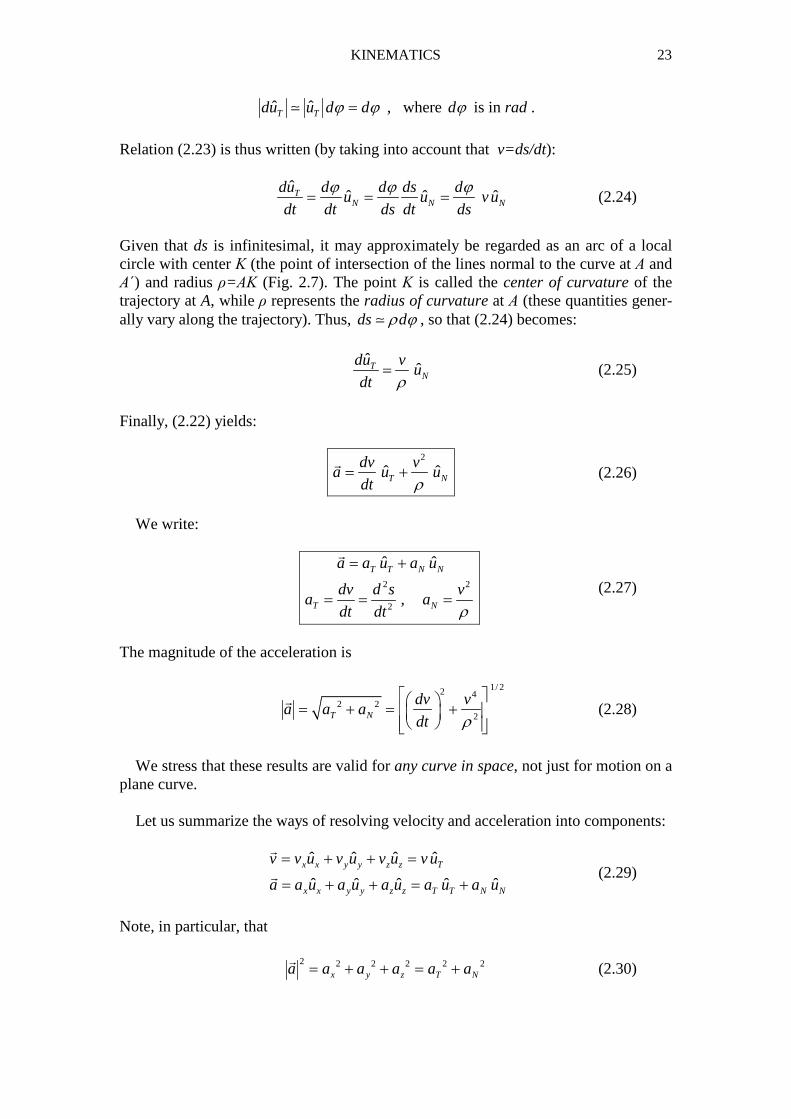
KINEMATICS 23
ˆ ˆT Tdu u d dϕ ϕ=≃ , where dϕ is in rad .
Relation (2.23) is thus written (by taking into account that v=ds/dt):
ˆ
ˆ ˆ ˆTN N N
du d d ds du u vu
dt dt ds dt ds
ϕ ϕ ϕ= = = (2.24)
Given that ds is infinitesimal, it may approximately be regarded as an arc of a local circle with center Κ (the point of intersection of the lines normal to the curve at Α and Α΄) and radius ρ=ΑΚ (Fig. 2.7). The point Κ is called the center of curvature of the trajectory at A, while ρ represents the radius of curvature at Α (these quantities gener-ally vary along the trajectory). Thus, ds dρ ϕ≃ , so that (2.24) becomes:
ˆ
ˆTN
du vu
dt ρ= (2.25)
Finally, (2.22) yields:
2
ˆ ˆT N
dv va u u
dt ρ= +�
(2.26)
We write:
2 2
2
ˆ ˆ
,
T T N N
T N
a a u a u
dv d s va a
dt dt ρ
= +
= = =
�
(2.27)
The magnitude of the acceleration is
1/ 22 42 2
2T N
dv va a a
dt ρ
= + = +
�
(2.28)
We stress that these results are valid for any curve in space, not just for motion on a plane curve. Let us summarize the ways of resolving velocity and acceleration into components:
ˆ ˆ ˆ ˆ
ˆ ˆ ˆ ˆ ˆx x y y z z T
x x y y z z T T N N
v v u v u v u vu
a a u a u a u a u a u
= + + =
= + + = +
�
� (2.29)
Note, in particular, that
2 2 2 2 2 2
x y z T Na a a a a a= + + = +�
(2.30)
24 CHAPTER 2
Special cases: 1. Uniform curvilinear motion: v=constant. We have:
2
ˆ ˆ0,T N N N
dv va a a u u
dt ρ= = = =
�
(2.31)
Note that in uniform motion the acceleration is normal to the velocity, in accordance with the conclusions of Sec. 2.4. [Exercise: Show that the distance s along the curve (Fig. 2.4) is given as a function of time by s=vt, where we assume that s=0 at t=0.] 2. Rectilinear motion: ˆ ˆ, , T xs x u uρ = ∞ = = . Hence,
2
ˆ ˆ ˆ ,
ˆ ˆ0 , .
T x x
N T T x
ds dxv u u vu
dt dt
v dva a a u u
dtρ
= = =
= = = =
�
�
In uniform rectilinear motion ( .v const=
�
) both aT and aN are zero, so that 0a =�
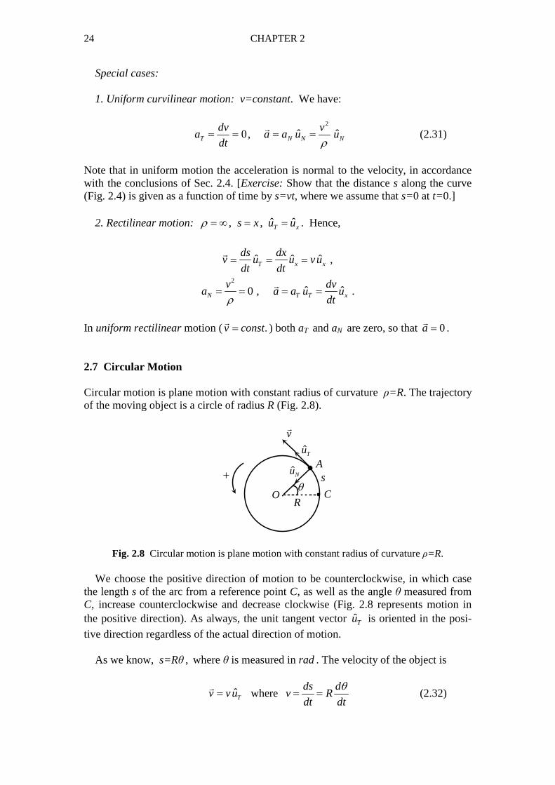
. 2.7 Circular Motion Circular motion is plane motion with constant radius of curvature ρ=R. The trajectory of the moving object is a circle of radius R (Fig. 2.8).
⋅OR
C
sA
ˆTu
ˆNu
v�
+θ
Fig. 2.8 Circular motion is plane motion with constant radius of curvature ρ=R. We choose the positive direction of motion to be counterclockwise, in which case the length s of the arc from a reference point C, as well as the angle θ measured from C, increase counterclockwise and decrease clockwise (Fig. 2.8 represents motion in the positive direction). As always, the unit tangent vector ˆTu is oriented in the posi-
tive direction regardless of the actual direction of motion. As we know, s=Rθ , where θ is measured in rad . The velocity of the object is
ˆ whereT
ds dv vu v R
dt dt
θ= = =�
(2.32)
KINEMATICS 25
(In general, v v= ±�
, depending on the direction of motion.) We define the angular
velocity
d
dt
θω = (2.33)
Then,
v Rω= (2.34)
The quantity ω is measured in rad / s = rad.s –1. Note that the sign of ω is the same as that of v and depends on the direction of motion. The acceleration of the object is
ˆ ˆT T N Na a u a u= +�
where
2 2( ),T N
dv d v Ra R a
dt dt R R
ω ω= = = = .
We define the angular acceleration
d
dt
ωα = (2.35)
We thus have:
2,T Na R a Rα ω= = (2.36)
The magnitude of the acceleration is
2 2 2 4T Na a a R α ω= + = +
�
(2.37)
In uniform circular motion the algebraic values v and ω are constant, so that, by (2.35) and (2.36), α=0 and aT =0. Hence, the acceleration is purely centripetal :
2
2ˆ ˆ ( , .)N N
va u R u v const
Rω ω= = =
�
(2.38)
By (2.33) and by taking into account that ω is constant, we have (assuming that θ=θ0 at t=0):
0 0 0
t td dt d dt dt
θ
θθ ω θ ω ω= ⇒ = = ⇒∫ ∫ ∫
0 tθ θ ω= + (2.39)
26 CHAPTER 2
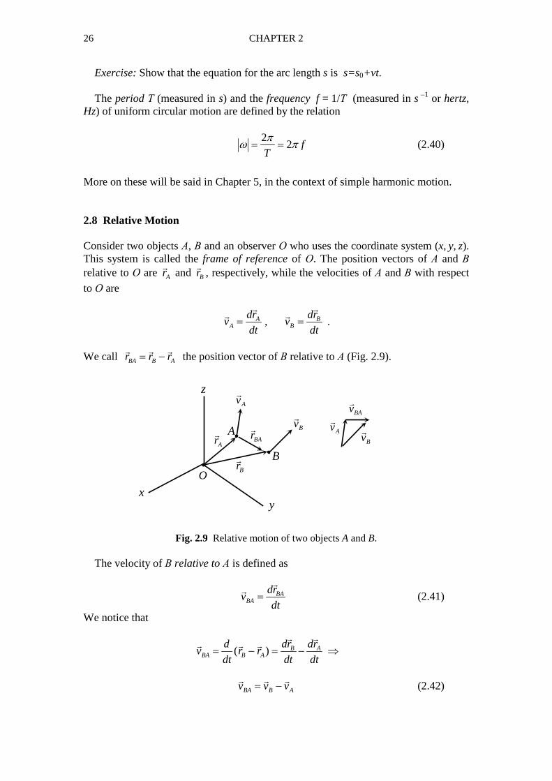
xy
z
O
Ar�
Br�
A
B
BAr�
Av�
Av�
Bv�
Bv�
BAv�
Exercise: Show that the equation for the arc length s is s=s0+vt. The period Τ (measured in s) and the frequency f = 1/Τ (measured in s –1 or hertz, Hz) of uniform circular motion are defined by the relation
2
2 fT
πω π= = (2.40)
More on these will be said in Chapter 5, in the context of simple harmonic motion. 2.8 Relative Motion Consider two objects Α, Β and an observer Ο who uses the coordinate system (x, y, z). This system is called the frame of reference of Ο. The position vectors of Α and Β relative to Ο are Ar
�
and Br�
, respectively, while the velocities of Α and Β with respect
to Ο are
,A BA B
dr drv v
dt dt= =� �
� �
.
We call BA B Ar r r= −
� � �
the position vector of Β relative to Α (Fig. 2.9).
Fig. 2.9 Relative motion of two objects A and B. The velocity of Β relative to Α is defined as
BABA
drv
dt=�
�
(2.41)
We notice that
( ) B ABA B A
d dr drv r r
dt dt dt= − = − ⇒
� �
� � �
BA B Av v v= −
� � �
(2.42)
KINEMATICS 27
Similarly, the velocity of Α relative to Β is AB A B BAv v v v= − = −
� � � �
(2.43)
In an analogous way we define the acceleration of Β relative to Α:
( )BA B ABA B A
dv d dv dva v v
dt dt dt dt= = − = − ⇒� � �
� � �
BA B A ABa a a a= − = −
� � � �
(2.44)
where
,A BA B
dv dva a
dt dt= =� �
� �
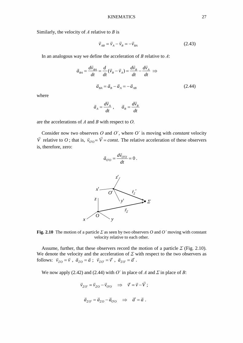
are the accelerations of Α and Β with respect to Ο. Consider now two observers Ο and Ο΄, where O΄ is moving with constant velocity
V�
relative to O ; that is, .O Ov V const′ = =��
The relative acceleration of these observers is, therefore, zero:
0O OO O
dva
dt′
′ = =�
�
.
i
i
•
O
O′
x y
z
x′
y′
z′
Σ
r�
rΣ ′�
Fig. 2.10 The motion of a particle Σ as seen by two observers O and O΄ moving with constant
velocity relative to each other. Assume, further, that these observers record the motion of a particle Σ (Fig. 2.10). We denote the velocity and the acceleration of Σ with respect to the two observers as follows: , ; ,O O O Ov v a a v v a aΣ Σ Σ Σ′ ′′ ′= = = =
� � � � � � � �
.
We now apply (2.42) and (2.44) with Ο΄ in place of Α and Σ in place of Β:
;
.
O O O O
O O O O
v v v v v V
a a a a a
Σ Σ
Σ Σ
′ ′
′ ′
′= − ⇒ = −
′= − ⇒ =
�� � � � �
� � � � �
28 CHAPTER 2
We thus arrive at an important conclusion:
A particle moves with the same acceleration with respect to two observers that maintain a constant velocity relative to each other (they do not accelerate with respect to each other).
In particular,
if the particle moves with constant velocity relative to one observer, it will also move with constant velocity relative to the other observer.
Stated differently, if the particle executes uniform rectilinear motion relative to one observer, it will execute the same kind of motion relative to the other observer.
References
1. A.F. Bermant, I.G. Aramanovich, Mathematical Analysis (Mir Publishers, 1975)
2. D.D. Berkey, Calculus, 2nd Edition (Saunders College, 1988)
29
CHAPTER 3
DYNAMICS OF A PARTICLE 3.1 The Law of Inertia The term point particle (or simply particle) refers to a body whose dimensions are so small that we may ignore its rotational motion (if any). But, even a body of finite di-mensions may be treated as a “particle” if its motion is purely translational (that is, if the body is not rotating). A particle is said to be free if (a) it is not subject to any interactions with the rest of the world (a case that is rather unrealistic!) or (b) the totality of its interactions some-how sum to zero (i.e., they cancel one another) so that the particle behaves as if it were subject to no interactions whatsoever. According to the Law of Inertia or New-ton’s First Law,
a free particle moves with constant velocity (i.e., has no acceleration) relative to any other free particle.
Therefore, a free particle either is in uniform rectilinear motion, or is at rest, relative to another free particle. Imagine now an observer who herself is a free particle (this is approximately true for someone who is at rest on the surface of the Earth). Such an observer is called an inertial observer and the system of coordinates or axes she uses is called an inertial frame of reference (or, simply, inertial frame). According to the law of inertia,
different inertial observers move with constant velocities (thus, do not accel-erate) relative to one another.
For example, the passenger in a train that moves with constant velocity relative to the ground is (approximately) an inertial observer and a fixed system of axes (x, y, z) in the train is an inertial frame of reference. On the basis of the law of inertia we may now give the following definition of an inertial reference frame:
An inertial frame of reference is any set of coordinates (or axes) relative to which a free particle either moves with constant velocity or is at rest. Thus, in an inertial frame a free particle does not accelerate.
We note that the observer who uses this frame is, by definition, at rest relative to it. A reference frame that accelerates with respect to an inertial frame is obviously not inertial. This is, e.g., the case with the Earth because of its daily rotation as well as its orbiting motion about the Sun (if we regard the latter as an almost inertial frame). However, since the acceleration of the Earth is relatively small compared to the accel-erations measured in typical terrestrial experiments, we may, for practical purposes,
30 CHAPTER 3
consider the Earth as an almost inertial frame. Hence, any observer moving on the surface of the Earth with constant velocity will be regarded as an inertial observer. 3.2 Momentum, Force, and Newton’s 2nd and 3rd Laws In an abstract sense, force represents the effort necessary in order to alter the state of motion of a body; in particular, in order to change the body’s velocity. The first idea that comes to mind is to quantitatively identify force with acceleration. We know from our experience, however, that different bodies generally require a different effort in order to acquire the same acceleration, or, the same velocity within the same period of time. (Try, e.g., to produce the same acceleration on a book and on a truck by push-ing them!) This happens because different bodies exhibit different inertia, that is, dif-ferent resistance to a change of their state of motion. This property must therefore be taken into account in the definition of force. To this end, we introduce a new physical quantity called linear momentum (or simply momentum) of a body: p mv=
� �
(3.1) where v
�
is the velocity of the body. The coefficient m is called mass and is a measure of the body’s inertia. Newton’s Second Law of Motion (we will often simply call it “Newton’s Law”), which is valid only in inertial frames of reference, in essence defines the force exerted on a body as the rate of change of the body’s momentum at time t :
dp
Fdt
=
��
(3.2)
If we make the assumption that the mass m is constant, then
( )dp d dv
mv mdt dt dt
= =
� �
�
.
Hence,
F ma=� �
(3.3)
where /a dv dt=� �
is the acceleration of the body at time t. We stress that the form (3.3) of Newton’s law is valid for a body of constant mass, as well as that relations (3.2) and (3.3) are valid on the assumption that the observer measuring the velocity and the acceleration of the body is an inertial observer. By using (3.3) and by taking into ac-count the conclusion at the end of Sec. 2.8, it is not hard to show that
the force on a particle is the same for all inertial observers (recall that inertial observers move with constant velocities relative to one another).
DYNAMICS OF A PARTICLE 31
The vector equation (3.3) is equivalent to three algebraic equations, one for each vector component. We write: ˆ ˆ ˆ ˆ ˆ ˆ, .x x y y z z x x y y z zF F u F u F u a a u a u a u= + + = + +
� �
Substituting these expressions into (3.3) and equating corresponding components in the two sides of this equation, in accordance with (1.8), we have: , ,x x y y z zF ma F ma F ma= = = (3.4)
Now, as implied by the law of inertia, the change of the state of motion of a body relative to an inertial observer requires an interaction of the body with the rest of the world. The force F
�
is precisely a measure of this interaction. If the body is not sub-ject to interactions (i.e., is a free “particle”) then F
�
=0 and it follows from (3.3) that the velocity of the body with respect to an inertial reference frame is constant (since the acceleration is zero). We thus conclude that the second law of motion is consistent with the law of inertia, provided that both these laws are examined from the point of view of an inertial frame of reference. It is tempting to argue that, according to the above discussion, the law of inertia is redundant since it appears to be just a special case of the second law:
Free particle ⇔ no interaction ⇔ no force ⇔ no acceleration ⇔ constant velocity. There is a subtle point, however: What kind of observer is entitled to conclude that a particle that appears to move with constant velocity (i.e., with no acceleration) is a free particle? Answer: Only an inertial observer, who uses an inertial frame of refer-ence! The purpose of the law of inertia is essentially to define these frames and guar-antee their existence. So, without the first law of motion, the second law would be-come indeterminate, if not altogether wrong, since it would appear to be valid relative to any observer regardless of his or her state of motion. One may say that the first law defines the “terrain” within which the second law acquires a meaning. Applying the latter law without taking the former one into account would be like trying to play soc-cer without possessing a soccer field!
According to (3.2), if a body is not subject to any force ( 0F =�
) its momentum p�
relative to an inertial frame is constant in time, since, in this case, / 0dp dt=
�
. As will be seen in Chapter 6, this is true, more generally, for any isolated system of particles, i.e., a system subject to no external interactions. For such a system the principle of conservation of momentum is valid:
The total momentum of a system of particles subject to no external forces is constant in time.
This principle is intimately related to a third law of motion. Consider a system of two particles subject only to their mutual interaction (there are no external forces). The total momentum of the system at times t and t+∆t is
32 CHAPTER 3
1 2 1 1 2 2
1 2 1 1 2 2
( ) ,
( ) .
P t p p m v m v
P t t p p m v m v
= + = +
′ ′ ′ ′+ ∆ = + = +
� � � � �
� � � � �
By conservation of momentum,
1 2 1 2( ) ( )P t P t t p p p p′ ′= + ∆ ⇒ + = + ⇒� � � � � �
1 1 2 2 1 2( )p p p p p p′ ′− = − − ⇔ ∆ = −∆� � � � � �
(3.5)
Hence,
1 2 1 2 1 2
0 0lim lim .t t
p p p p dp dp
t t t t dt dt∆ → ∆ →
∆ ∆ ∆ ∆= − ⇒ = − ⇒ = −
∆ ∆ ∆ ∆
� � � � � �
But, by (3.2),
1 212 21,
dp dpF F
dt dt= =
� �� �
where 12F
�
is the internal force exerted on particle 1 by its interaction with particle 2,
while 21F�
is the force on particle 2 due to its interaction with particle 1. Thus, finally,
12 21F F= −� �
(3.6)
Relation (3.6) expresses Newton’s Third Law or Law of Action and Reaction. Note that this law is equivalent to the principle of conservation of momentum, which prin-ciple, in turn, constitutes the generalization of the law of inertia for a system of parti-cles. Taking into account that Newton’s second law (in essence, the definition of the concept of force) also is a logical extension of the first law, we can appreciate the great importance of the law of inertia in the axiomatic foundation of Newtonian Me-chanics! (For a discussion of the axiomatic basis of Newtonian Mechanics, see [1].) You may have noticed that we defined momentum, which depends explicitly on mass, without previously giving a definition of mass itself. We will now describe a method for determining mass, based on the principle of conservation of momentum. Consider again an isolated system (i.e., a system subject to no external forces) con-sisting of two particles of masses m1, m2, which somehow interact with each other (e.g., they collide or, if they are electrically charged, they exert Coulomb forces on each other, etc.). Assume that, within a time interval ∆t, the momenta of m1 and m2 change by 1p∆
�
and 2p∆�
, respectively. According to (3.5), 1 2p p∆ = −∆� �
or
1 1 2 2m v m v∆ = − ∆
� �
(3.7)
In terms of magnitudes,
DYNAMICS OF A PARTICLE 33
1 1 2 2m v m v∆ = ∆ ⇒� �
2 1
1 2
m v
m v
∆=∆
�
� (3.8)
As experiment shows, the ratio of magnitudes on the right-hand side of (3.8) always assumes the same value for given particles m1 and m2 , regardless of the kind or the duration of their interaction. Moreover, the vectors 1v∆
�
and 2v∆�
are found to be in
opposite directions, in accordance with (3.7). These observations verify that to each particle in the system there corresponds a constant quantity m, its mass, such that the sum 1 1 2 2m v m v+
� �
retains a constant value when the particles are subject only to their
mutual interaction. This constitutes an experimental verification of conservation of momentum. Now, relation (3.8) allows us to determine the ratio m2/m1 experimentally by meas-uring the ratio of magnitudes of 1v∆
�
and 2v∆�
. Hence, by arbitrarily assigning unit
value to the mass of particle 1, we can determine the mass of particle 2 as follows: We allow the two particles to interact for a time interval ∆t ; then we measure the (vector) changes of their velocities within this interval and we calculate the ratio of magni-tudes of these changes. The result yields the mass m2 of particle 2 numerically (since, by definition, m1 is a unit mass). In a similar way, we determine the mass m of any particle by allowing this particle to interact with a particle of known mass. By measur-ing the instantaneous acceleration a
�
of m we then find the corresponding instantane-ous force F
�
on this particle by using Newton’s law (3.3). In the S.I. system of units, the unit of mass is 1kg=103 g while the unit of force is 1Newton=1N=1kg.m.s –2 . Assume now that a body of mass m is subject to various interactions with its sur-
roundings, which interactions are represented quantitatively by the forces 1 2, ,F F� �
⋯ .
The vector sum
1 2ii
F F F F≡ = + +∑ ∑� � � �
⋯
is the resultant force (or total force) acting on the body. Newton’s second law then takes on the form:
dp
F madt
= =∑�
� �
(3.9)
Let ax , ay , az be the components of the acceleration a�
of the body. According to (1.10), the components of the resultant force FΣ
�
are ΣFx , ΣFy , ΣFz , where ΣFx is the
sum of the x-components of the individual forces 1 2, ,F F� �
⋯, and similarly for ΣFy and
ΣFz . By equating corresponding components on the two sides of (3.9), we have:
34 CHAPTER 3
, ,x x y y z zF ma F ma F ma= = =∑ ∑ ∑ (3.10)
As an example, assume that a body of mass m=2kg is subject to the forces
1 (3,1, 1)F N≡ −�
and 2 ( 1,3, 1)F N≡ − −�
. The resultant force is
1 2 (2,4, 2)F F F N= + ≡ −∑� � �
so that ΣFx=2N, ΣFy=4N, ΣFz= −2N. By (3.10) we find the acceleration of the body: 2( , , ) (1,2, 1)x y za a a a m s−≡ ≡ − ⋅
�
.
A body is said to be in equilibrium if the total force on it is zero: 0FΣ =
�
. Note that by “equilibrium” we do not necessarily mean rest ( 0v =
�
). According to (3.9), a body is in a state of equilibrium if it does not accelerate ( 0)a =
�
relative to an inertial ob-server. If, however, the body is initially at rest at an equilibrium position where the total force on it vanishes, then it remains at rest there. Conversely, a body may be momentarily at rest without being in a state of equilib-rium. The total force acting on it will then cause an acceleration that will put the body back in motion at the very next moment. For example, if we throw a stone straight upward, it will stop instantaneously as soon as it reaches a maximum height and then it will start moving downward immediately, under the action of gravity. Another ex-ample of momentary rest is that of a pendulum bob at the highest point of its path. We noted earlier that a body of finite dimensions can be treated as if it were a point particle if its motion is purely translational (i.e., the body is not subject to rotation). Such a motion depends only on the resultant force on the body, regardless of the loca-tion of the points of action of the various individual forces that act on this body. On the contrary, as will be seen in Chapter 7, the points of action of these forces are im-portant when one considers rotational motion, as this motion is determined by the to-tal external torque on the body. 3.3 Force of Gravity Near the surface of the Earth and in the absence of air resistance, all bodies fall to-ward the ground with a common acceleration g
�
, called the acceleration of gravity
and having a magnitude 29.8g m s−⋅≃ . The force of gravitational attraction between a body and the Earth is called the weight w
�
of the body. If m is the mass of the body, then, by Newton’s second law, w mg=
� �
(3.11) For larger distances from the surface of the Earth, the value of g (hence also the weight of a body) varies as a function of the distance from the Earth. We call M and R the mass and the radius of the Earth, respectively, and we let h be a given height above the surface of the Earth. We would like to determine the value of g at this height. According to Newton’s Law of Gravity, the magnitude of the gravitational force on a body of mass m, located at a height h above the Earth, is
DYNAMICS OF A PARTICLE 35
2( )
Mmw G
R h=
+ (3.12)
where G is a constant, the value of which is experimentally determined to be G = 6.673 × 10 –11 N.m2.kg–2 . Taking into account that w=mg , we find that
2( )
GMg
R h=
+ (3.13)
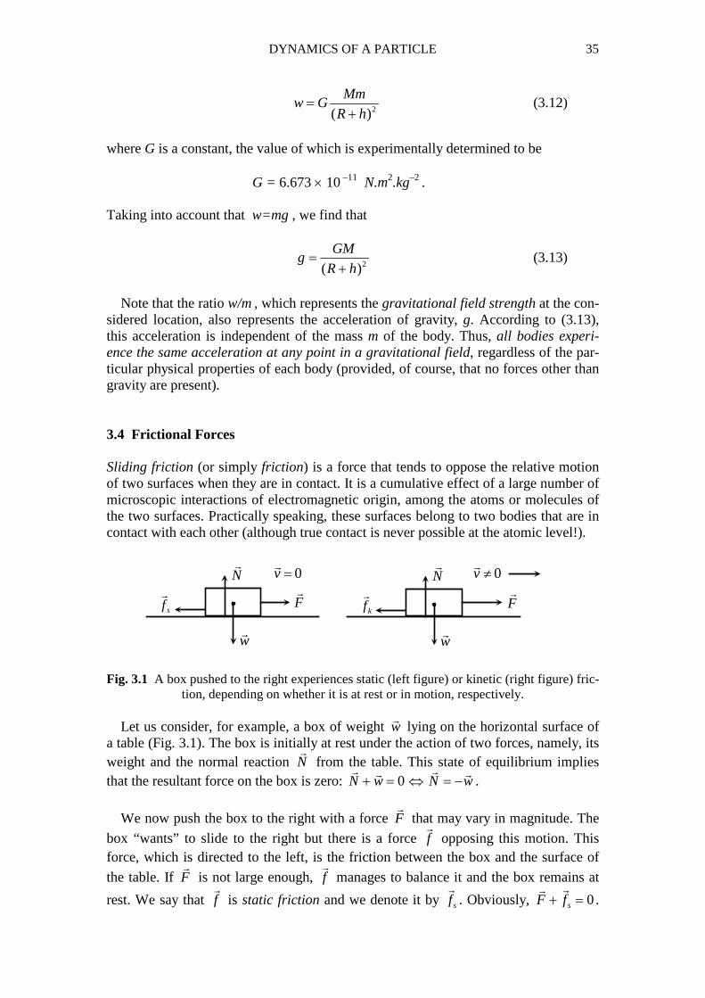
Note that the ratio w/m , which represents the gravitational field strength at the con-sidered location, also represents the acceleration of gravity, g. According to (3.13), this acceleration is independent of the mass m of the body. Thus, all bodies experi-ence the same acceleration at any point in a gravitational field, regardless of the par-ticular physical properties of each body (provided, of course, that no forces other than gravity are present). 3.4 Frictional Forces Sliding friction (or simply friction) is a force that tends to oppose the relative motion of two surfaces when they are in contact. It is a cumulative effect of a large number of microscopic interactions of electromagnetic origin, among the atoms or molecules of the two surfaces. Practically speaking, these surfaces belong to two bodies that are in contact with each other (although true contact is never possible at the atomic level!). Fig. 3.1 A box pushed to the right experiences static (left figure) or kinetic (right figure) fric-
tion, depending on whether it is at rest or in motion, respectively. Let us consider, for example, a box of weight w
�
lying on the horizontal surface of a table (Fig. 3.1). The box is initially at rest under the action of two forces, namely, its weight and the normal reaction N
�
from the table. This state of equilibrium implies that the resultant force on the box is zero: 0N w N w+ = ⇔ = −
� �� �
. We now push the box to the right with a force F
�
that may vary in magnitude. The
box “wants” to slide to the right but there is a force f�
opposing this motion. This force, which is directed to the left, is the friction between the box and the surface of
the table. If F�
is not large enough, f�
manages to balance it and the box remains at
rest. We say that f�
is static friction and we denote it by sf�
. Obviously, 0sF f+ =��
.
w�
N�
F�
kf�
0v ≠�
w�
N�
F�
sf�
0v =�

36 CHAPTER 3
Depending on the applied force F�
, the force sf�
varies from zero (when 0F =�
) to a
maximum value ,maxsf�
.
When F�
exceeds ,maxsf�
in magnitude, the box is set in motion on the table, accel-
erating to the right. The frictional force then decreases from ,maxsf�
to a new, constant
value kf�
(also directed to the left) that opposes the motion; it is called kinetic friction.
The total force on the box during the motion is tot kF F f= +�� �
. If we assume that the
box moves in the positive direction of the x-axis, then
ˆ ˆ ˆ ˆ,x x k k x k xF F u F u f f u f u= = = − = −� �� �
so that
ˆ ˆ ˆ( ) ( )tot x k x k xF F u f u F f u= + − = −�
(3.14)
By dividing totF�
with the mass m of the box we find the acceleration a�
of the box. In
the case where F= fk the resultant force totF�
is zero and the box moves with constant
velocity. If we withdraw the applied force F�
, the kinetic friction kf�
decelerates the
body until the latter comes to a halt. As found experimentally, the magnitude fs,max of maximum static friction, as well as the magnitude fk of kinetic friction, is proportional to the magnitude N of the nor-mal force pressing one surface against the other. Thus, the possible values of static friction are ,max0 s s sf f Nµ≤ ≤ = (3.15)
while the value of kinetic friction is k kf Nµ= (3.16)
where µs and µk are the coefficients of friction (static and kinetic, respectively), with µk < µs . Note that µs and µk are dimensionless quantities (i.e., pure numbers). These coefficients depend on the nature of the two surfaces and typically vary between 0.05 and 1.5 . We now describe an experimental method for determining the coefficients of fric-tion between two surfaces:
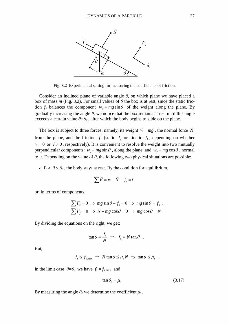
DYNAMICS OF A PARTICLE 37
f�
N�
w�
ˆxu
ˆ yu
θ
θ
Fig. 3.2 Experimental setting for measuring the coefficients of friction.
Consider an inclined plane of variable angle θ, on which plane we have placed a box of mass m (Fig. 3.2). For small values of θ the box is at rest, since the static fric-tion fs balances the component sinxw mg θ= of the weight along the plane. By
gradually increasing the angle θ, we notice that the box remains at rest until this angle exceeds a certain value θ=θc , after which the body begins to slide on the plane. The box is subject to three forces; namely, its weight w mg=
� �
, the normal force N�
from the plane, and the friction f�
(static sf�
or kinetic kf�
, depending on whether
0v =�
or 0v ≠�
, respectively). It is convenient to resolve the weight into two mutually perpendicular components: sinxw mg θ= , along the plane, and cosyw mg θ= , normal
to it. Depending on the value of θ, the following two physical situations are possible: a. For θ ≤ θc , the body stays at rest. By the condition for equilibrium,
0sF w N f= + + =∑�� ��
or, in terms of components,
0 sin 0 sin ,
0 cos 0 cos .
x s s
y
F mg f mg f
F N mg mg N
θ θ
θ θ
= ⇒ − = ⇒ =
= ⇒ − = ⇒ =
∑∑
By dividing the equations on the right, we get:
tan tanss
ff N
Nθ θ= ⇒ = .
But,
,max tan tans s s sf f N Nθ µ θ µ≤ ⇒ ≤ ⇒ ≤ .
In the limit case θ=θc we have fs = fs,max and tan c sθ µ= (3.17)
By measuring the angle θc we determine the coefficient µs .
38 CHAPTER 3
b. For θ > θc the body accelerates along the inclined plane; the friction is now ki-netic. If we gradually decrease the angle θ we will find some value θc΄ < θc for which the body moves with constant velocity. By Newton’s law and by taking into account that the body does not accelerate, we have:
0kF w N f= + + =∑�� ��
.
Taking components, as before, we find: sin , cosc k k cmg ΄ f N mg ΄ Nθ µ θ= = = .
By dividing these equations, we get: tan c k΄θ µ= (3.18)
The experimental fact that θc΄ < θc combined with (3.17) and (3.18) indicates that µk < µs . This means that fk < fs,max . 3.5 Systems with Variable Mass In the case of a point particle or a body of constant mass m, Newton’s second law may be expressed in two equivalent ways:
( ) ( )dp
F a F ma bdt
= ⇔ =
�� � �
However, in the case of a system of particles relation (b) is not applicable, since it is not clear what exactly the acceleration vector a
�
represents (in Chapter 6 we will see that this relation acquires a meaning by introducing the concept of the center of mass). Thus, in the mechanics of systems we generally use relation (a), in the form
dP
Fdt
=
�
�
(3.19)
where P
�
is the total momentum of the system at time t, and where F�
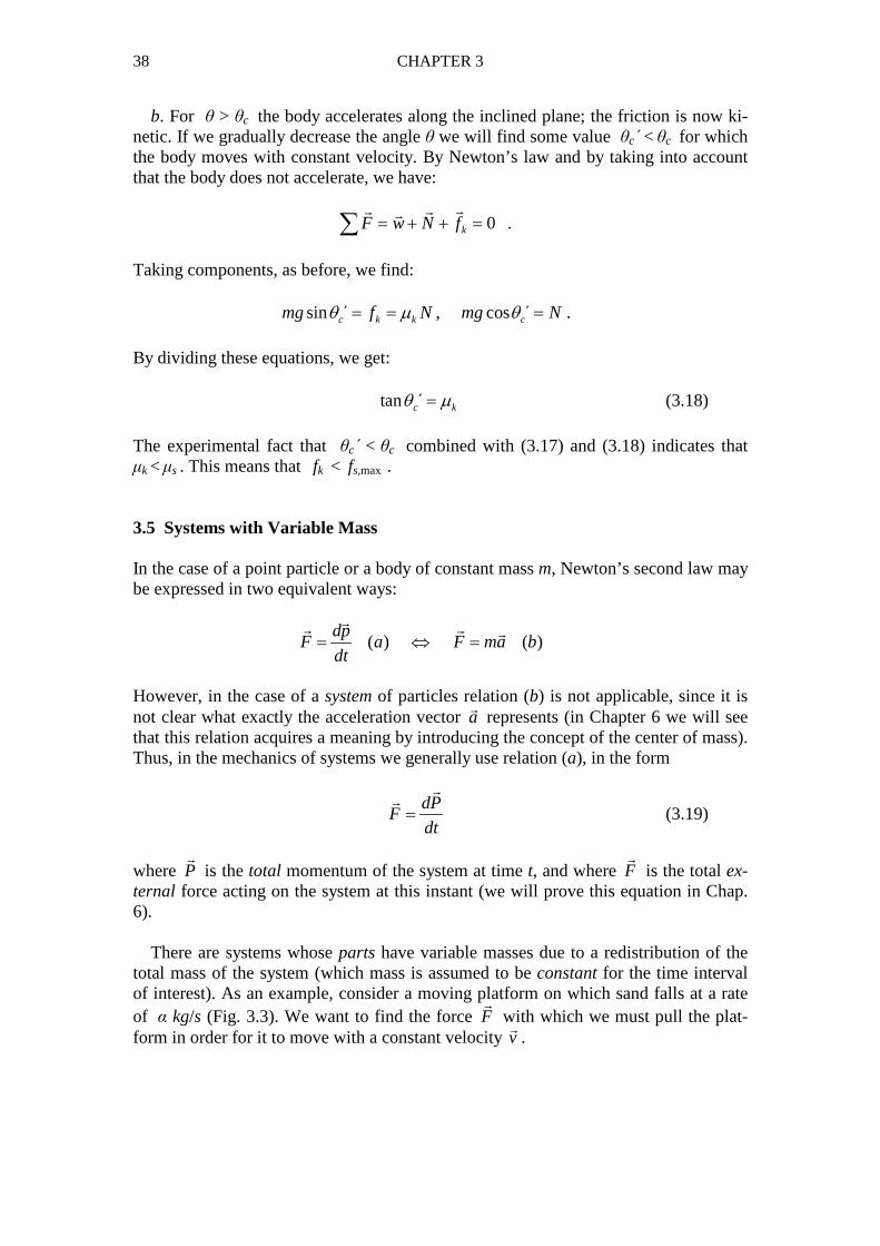
is the total ex-ternal force acting on the system at this instant (we will prove this equation in Chap. 6). There are systems whose parts have variable masses due to a redistribution of the total mass of the system (which mass is assumed to be constant for the time interval of interest). As an example, consider a moving platform on which sand falls at a rate of α kg/s (Fig. 3.3). We want to find the force F
�
with which we must pull the plat-form in order for it to move with a constant velocity v
�
.
DYNAMICS OF A PARTICLE 39
⋅⋅⋅⋅ ⋅⋅⋅⋅
⋅⋅ ⋅⋅⋅⋅⋅⋅⋅ ⋅⋅
⋅
⋅ ⋅ ⋅⋅⋅⋅⋅⋅⋅⋅ ⋅ ⋅ ⋅ ⋅ ⋅⋅⋅⋅ ⋅⋅ ⋅⋅
⋅ ⋅⋅ ⋅ ⋅⋅ ⋅ ⋅
⋅⋅⋅
⋅⋅
F�
mM
.v const=�
Fig. 3.3 A moving platform on which sand falls at a constant rate.
Let Μ be the (constant) mass of the platform. We call m the mass of the sand that has already fallen on the platform at time t, and we let dm be the additional mass of sand that falls within an infinitesimal time interval dt. According to the data of the problem,
( / )dm
kg sdt
α= (3.20)
Now, to use relation (3.19) we must first decide to which system of masses it will be applied. The total mass of this system will be constant in the time interval dt, al-though this mass will suffer redistribution. As a “system” we consider the three masses M, m and dm. At time t the mass (M+m) moves with velocity v
�
while the ve-locity of dm is zero (this latter quantity has not yet fallen onto the platform). At time t+dt, however, the total mass (M+m+dm) moves with velocity v
�
. If ( )P t�
and
( )P t dt+�
is the total momentum of the system at these two instants, we have: ( ) ( ) ( ) 0 , ( ) ( )P t M m v dm P t dt M m dm v= + + ⋅ + = + +
� �� �
.
The change of the system’s momentum within the time interval dt is
( ) ( ) ( )dP dm
dP P t dt P t dm v v vdt dt
α= + − = ⇒ = =
�
� � � � � �
where we have used (3.20). According to (3.19), /dP dt
�
represents the total external force on the system at time t, which force is none other than the force F
�
we apply on the platform. Hence,
dm
F v vdt
α= =� � �
(3.21)
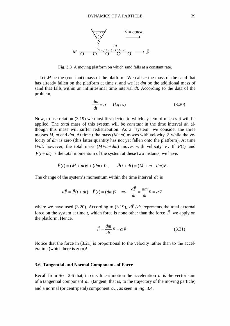
Notice that the force in (3.21) is proportional to the velocity rather than to the accel-eration (which here is zero)! 3.6 Tangential and Normal Components of Force Recall from Sec. 2.6 that, in curvilinear motion the acceleration a
�
is the vector sum of a tangential component Ta
�
(tangent, that is, to the trajectory of the moving particle)
and a normal (or centripetal) component Na�
, as seen in Fig. 3.4.
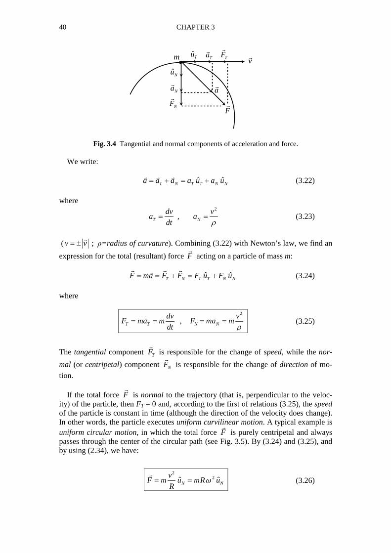
40 CHAPTER 3
•m ˆTu
ˆNu
Ta�
Na�
TF�
NF�
v�
a�
F�
Fig. 3.4 Tangential and normal components of acceleration and force. We write: ˆ ˆT N T T N Na a a a u a u= + = +
� � �
(3.22)
where
2
,T N
dv va a
dt ρ= = (3.23)
(v v= ±
�
; ρ=radius of curvature). Combining (3.22) with Newton’s law, we find an
expression for the total (resultant) force F�
acting on a particle of mass m: ˆ ˆT N T T N NF ma F F F u F u= = + = +
� � ��
(3.24)
where
2
,T T N N
dv vF ma m F ma m
dt ρ= = = = (3.25)
The tangential component TF�
is responsible for the change of speed, while the nor-
mal (or centripetal) component NF�
is responsible for the change of direction of mo-
tion. If the total force F
�
is normal to the trajectory (that is, perpendicular to the veloc-ity) of the particle, then FT = 0 and, according to the first of relations (3.25), the speed of the particle is constant in time (although the direction of the velocity does change). In other words, the particle executes uniform curvilinear motion. A typical example is uniform circular motion, in which the total force F
�
is purely centripetal and always passes through the center of the circular path (see Fig. 3.5). By (3.24) and (3.25), and by using (2.34), we have:
2
2ˆ ˆN N
vF m u mR u
Rω= =
�
(3.26)
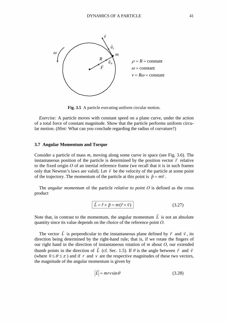
DYNAMICS OF A PARTICLE 41
•
•
v�
ˆTu
ˆNuF�
mR
ω
Fig. 3.5 A particle executing uniform circular motion. Exercise: A particle moves with constant speed on a plane curve, under the action of a total force of constant magnitude. Show that the particle performs uniform circu-lar motion. (Hint: What can you conclude regarding the radius of curvature?) 3.7 Angular Momentum and Torque Consider a particle of mass m, moving along some curve in space (see Fig. 3.6). The instantaneous position of the particle is determined by the position vector r
�
relative to the fixed origin Ο of an inertial reference frame (we recall that it is in such frames only that Newton’s laws are valid). Let v
�
be the velocity of the particle at some point of the trajectory. The momentum of the particle at this point is p mv=
� �
. The angular momentum of the particle relative to point Ο is defined as the cross product
( )L r p m r v= × = ×� � � � �
(3.27) Note that, in contrast to the momentum, the angular momentum L
�
is not an absolute quantity since its value depends on the choice of the reference point Ο. The vector L
�
is perpendicular to the instantaneous plane defined by r�
and v�
, its direction being determined by the right-hand rule; that is, if we rotate the fingers of our right hand in the direction of instantaneous rotation of m about Ο, our extended thumb points in the direction of L
�
(cf. Sec. 1.5). If θ is the angle between r�
and v�
(where 0 θ π≤ ≤ ) and if r and v are the respective magnitudes of these two vectors, the magnitude of the angular momentum is given by
sinL mrv θ=�
(3.28)
constant
constant
constant
R
v R
ρ
ω
ω
= =
=
= =
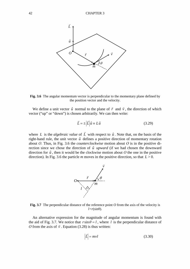
42 CHAPTER 3
u
L�
r� v
�O
mθ•
•
Fig. 3.6 The angular momentum vector is perpendicular to the momentary plane defined by
the position vector and the velocity. We define a unit vector u normal to the plane of r
�
and v�
, the direction of which vector (“up” or “down”) is chosen arbitrarily. We can then write:
ˆ ˆL L u Lu= ± ≡� �
(3.29)
where L is the algebraic value of L
�
with respect to u . Note that, on the basis of the right-hand rule, the unit vector u defines a positive direction of momentary rotation about Ο. Thus, in Fig. 3.6 the counterclockwise motion about Ο is in the positive di-rection since we chose the direction of u upward (if we had chosen the downward direction for u , then it would be the clockwise motion about Ο the one in the positive direction). In Fig. 3.6 the particle m moves in the positive direction, so that L > 0. Fig. 3.7 The perpendicular distance of the reference point O from the axis of the velocity is
l=r (sinθ). An alternative expression for the magnitude of angular momentum is found with the aid of Fig. 3.7. We notice that sinr lθ = , where l is the perpendicular distance of Ο from the axis of v
�
. Equation (3.28) is thus written:
L mvl=�
(3.30)
•
•
Or�
mθ
l
v�
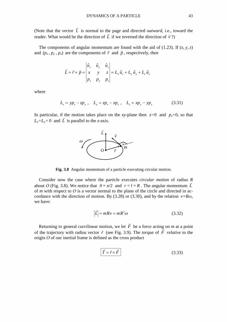
DYNAMICS OF A PARTICLE 43
(Note that the vector L�
is normal to the page and directed outward, i.e., toward the reader. What would be the direction of L
�
if we reversed the direction of v�
?) The components of angular momentum are found with the aid of (1.23). If (x, y, z) and (px , py , pz) are the components of r
�
and p�
, respectively, then
ˆ ˆ ˆ
ˆ ˆ ˆx y z
x x y y z z
x y z
u u u
L r p x y z L u L u L u
p p p
= × = = + +� � �
where , ,x z y y x z z y xL yp zp L zp xp L xp yp= − = − = − (3.31)
In particular, if the motion takes place on the xy-plane then z=0 and pz=0, so that Lx=Ly= 0 and L
�
is parallel to the z-axis.
•O
ω
r� m
v�L
�
•
Fig. 3.8 Angular momentum of a particle executing circular motion. Consider now the case where the particle executes circular motion of radius R about Ο (Fig. 3.8). We notice that θ = π/2 and r = l = R . The angular momentum L
�
of m with respect to Ο is a vector normal to the plane of the circle and directed in ac-cordance with the direction of motion. By (3.28) or (3.30), and by the relation v=Rω, we have:
2L mRv mRω= =�
(3.32)
Returning to general curvilinear motion, we let F
�
be a force acting on m at a point of the trajectory with radius vector r
�
(see Fig. 3.9). The torque of F�
relative to the origin Ο of our inertial frame is defined as the cross product
T r F= � ��
(3.33)
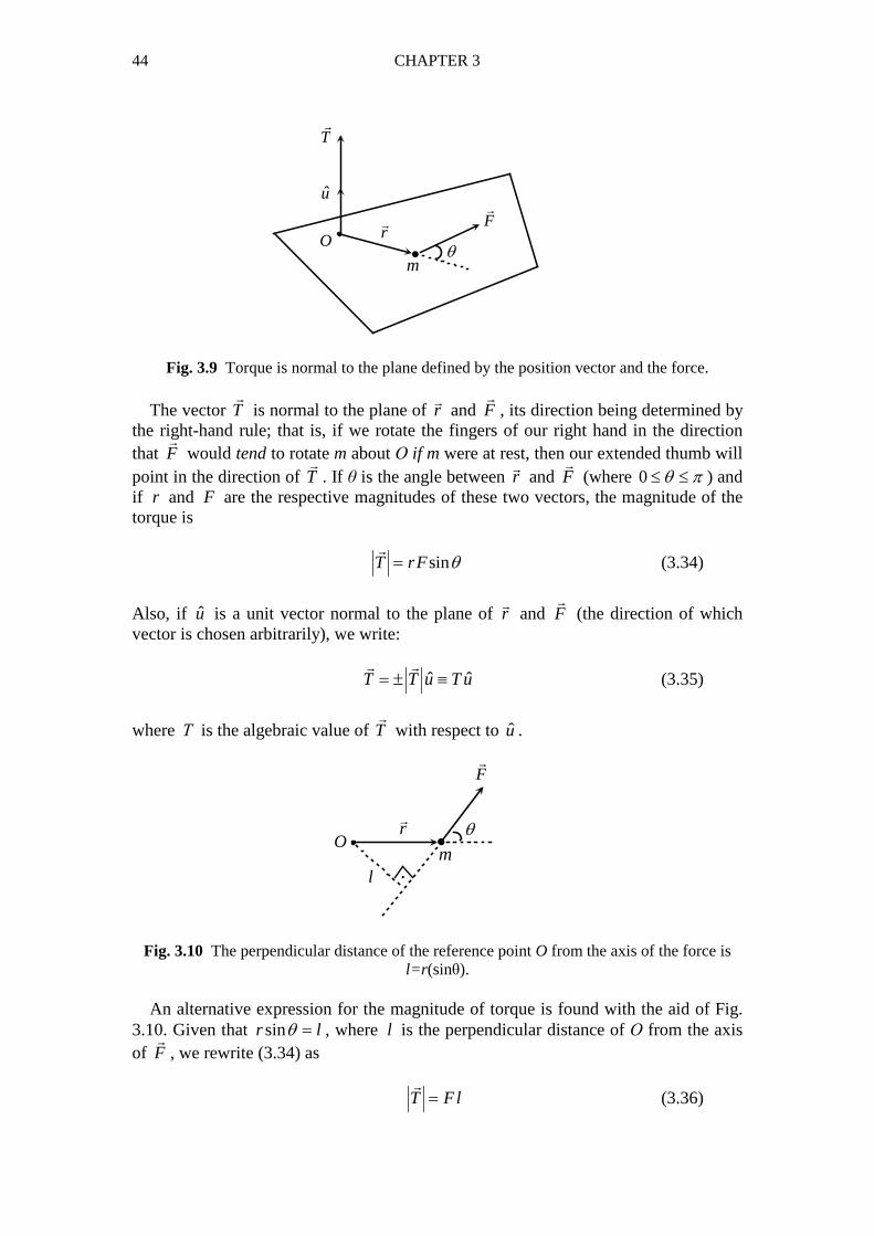
44 CHAPTER 3
Fig. 3.9 Torque is normal to the plane defined by the position vector and the force. The vector T
�
is normal to the plane of r�
and F�
, its direction being determined by the right-hand rule; that is, if we rotate the fingers of our right hand in the direction that F
�
would tend to rotate m about Ο if m were at rest, then our extended thumb will point in the direction of T
�
. If θ is the angle between r�
and F�
(where 0 θ π≤ ≤ ) and if r and F are the respective magnitudes of these two vectors, the magnitude of the torque is
sinT rF θ=�
(3.34)
Also, if u is a unit vector normal to the plane of r
�
and F�
(the direction of which vector is chosen arbitrarily), we write:
ˆ ˆT T u T u= ± ≡� �
(3.35)
where Τ is the algebraic value of T
�
with respect to u .
Fig. 3.10 The perpendicular distance of the reference point O from the axis of the force is
l=r (sinθ). An alternative expression for the magnitude of torque is found with the aid of Fig. 3.10. Given that sinr lθ = , where l is the perpendicular distance of Ο from the axis of F�
, we rewrite (3.34) as
T Fl=�
(3.36)
•O
u
T�
r�
mθ
F�
•
•
Or�
mθ
l
F�
DYNAMICS OF A PARTICLE 45
Finally, the components of T�
are (show this) , ,x z y y x z z y xT yF zF T zF xF T xF yF= − = − = − (3.37)
Between angular momentum and total torque there exists a relation analogous to the relation /F dp dt=
� �
between linear momentum and total force. Differentiating the angular momentum (3.27) with respect to t, we have:
( )dL d dr dp
r p p rdt dt dt dt
= × = × + ×
� � �
� � � �
(note carefully that, upon differentiation, the order in which r
�
and p�
appear must be preserved, since the cross product is not commutative). But,
( ) ( ) 0dr
p v p v mv m v vdt× = × = × = × =
�
� � � � � � �
.
Furthermore, by Newton’s law (3.2) and by the definition (3.33) of torque,
dp
r r F Tdt
× = × =
�� �� �
where F
�
is assumed here to be the resultant force on m. Thus, finally,
dL
Tdt
=
�
�
(3.38)
Exercise: Show that the torque T
�
of the resultant force on m is equal to the vector sum of the torques of all forces acting on m (cf. Appendix A). Note that, in equation (3.38), L
�
and T�
must be taken with respect to the same point Ο, which is the origin of our inertial frame of reference. Note also that (3.38) is an immediate consequence of Newton’s law (3.2); it does not represent a new funda-mental principle of Mechanics. In the case where 0T =
�
, (3.38) yields:
0 constantdL
Ldt
= ⇒ =
�
�
.
This leads us to the principle of conservation of angular momentum:
When the torque of the total force on a particle, relative to some point, is zero, the angular momentum of the particle relative to this point is constant in time.
Even if such a point exists, however, there may be other points relative to which nei-ther the torque of the total force vanishes, nor the angular momentum is constant!

46 CHAPTER 3
Exercise: An electric charge Q is permanently located at the origin Ο of our coor-dinate system, while another charge q may move freely in space. Ignoring the weight of q, as well as the air resistance, show that the angular momentum of q relative to Ο is constant. Would the same be true for the angular momentum of q relative to a dif-ferent point Ο΄ ? (Remember that the location of Q is fixed at O!) 3.8 Central Forces Consider a particle of mass m, moving on a curved path under the action of a total force F
�
. The instantaneous position of m is determined by the position vector r�
with respect to the origin Ο of an inertial reference frame. In general, the force F
�
varies in space (and, in particular, along the path of m). This force is thus a function of r
�
. We say that the particle m is moving in a force field F
�
= F�
( r�
) . Imagine now that we are able to choose a reference point Ο (see Fig. 3.11) such that
1. the line of action of F�
always passes through Ο, regardless of the position of the particle m in space;
2. the magnitude of F�
depends only on the distance r r=�
of m from Ο.
By defining the unit vector ru in the direction of r
�
,
ˆr
r ru
r r= =
� �
� ,
we can express both these conditions mathematically as follows:
( )
ˆ( ) r
F rF F r u r
r= =� �
(3.39)
where ( )F r F= ±�
is an algebraic value, the sign of which depends on the relative
orientation of F�
with respect to r�
. A force (more correctly, a force field) of the form (3.39) is called a central force with center at Ο.
Fig. 3.11 A particle subject to a central force.
Oˆru r
� F�
v�
m
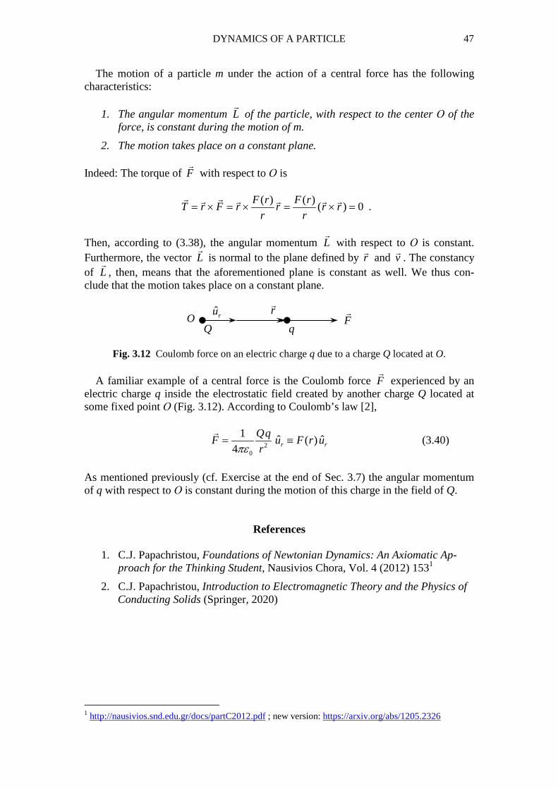
DYNAMICS OF A PARTICLE 47
The motion of a particle m under the action of a central force has the following characteristics:
1. The angular momentum L�
of the particle, with respect to the center Ο of the force, is constant during the motion of m.
2. The motion takes place on a constant plane. Indeed: The torque of F
�
with respect to Ο is
( ) ( )
( ) 0F r F r
T r F r r r rr r
= × = × = × =� �� � � � �
.
Then, according to (3.38), the angular momentum L
�
with respect to Ο is constant. Furthermore, the vector L
�
is normal to the plane defined by r�
and v�
. The constancy of L�
, then, means that the aforementioned plane is constant as well. We thus con-clude that the motion takes place on a constant plane.
Fig. 3.12 Coulomb force on an electric charge q due to a charge Q located at O. A familiar example of a central force is the Coulomb force F
�
experienced by an electric charge q inside the electrostatic field created by another charge Q located at some fixed point Ο (Fig. 3.12). According to Coulomb’s law [2],
2
0
1ˆ ˆ( )
4 r r
QqF u F r u
rπε= ≡�
(3.40)
As mentioned previously (cf. Exercise at the end of Sec. 3.7) the angular momentum of q with respect to Ο is constant during the motion of this charge in the field of Q.
References
1. C.J. Papachristou, Foundations of Newtonian Dynamics: An Axiomatic Ap-proach for the Thinking Student, Nausivios Chora, Vol. 4 (2012) 1531
2. C.J. Papachristou, Introduction to Electromagnetic Theory and the Physics of Conducting Solids (Springer, 2020)
1 http://nausivios.snd.edu.gr/docs/partC2012.pdf ; new version: https://arxiv.org/abs/1205.2326
F�ˆru r
�
OQ q
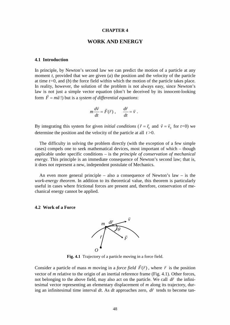
48
CHAPTER 4
WORK AND ENERGY 4.1 Introduction In principle, by Newton’s second law we can predict the motion of a particle at any moment t, provided that we are given (a) the position and the velocity of the particle at time t=0, and (b) the force field within which the motion of the particle takes place. In reality, however, the solution of the problem is not always easy, since Newton’s law is not just a simple vector equation (don’t be deceived by its innocent-looking form F ma=
� �
!) but is a system of differential equations:
( ) , .dv dr
m F r vdt dt
= =
� �� � �
By integrating this system for given initial conditions ( 0r r=
� �
and 0v v=� �
for t=0) we
determine the position and the velocity of the particle at all t >0. The difficulty in solving the problem directly (with the exception of a few simple cases) compels one to seek mathematical devices, most important of which – though applicable under specific conditions – is the principle of conservation of mechanical energy. This principle is an immediate consequence of Newton’s second law; that is, it does not represent a new, independent postulate of Mechanics. An even more general principle – also a consequence of Newton’s law – is the work-energy theorem. In addition to its theoretical value, this theorem is particularly useful in cases where frictional forces are present and, therefore, conservation of me-chanical energy cannot be applied. 4.2 Work of a Force
•
O
r�
m dr� v
�
θ
F�
Fig. 4.1 Trajectory of a particle moving in a force field.
Consider a particle of mass m moving in a force field ( )F r
� �
, where r�
is the position vector of m relative to the origin of an inertial reference frame (Fig. 4.1). Other forces, not belonging to the above field, may also act on the particle. We call dr
�
the infini-tesimal vector representing an elementary displacement of m along its trajectory, dur-ing an infinitesimal time interval dt. As dt approaches zero, dr
�
tends to become tan-

WORK AND ENERGY 49
gent to the trajectory; that is, it tends to acquire the direction of the velocity v�
of the particle. We define the elementary work of the force F
�
, for the displacement dr�
of m, as the dot product cosdW F dr Fds θ= ⋅ =
� �
(4.1)
where F F=�
and ds dr=�
, with the understanding that, within an infinitesimal time
interval, ds may approximately be considered equal to the length of an infinitesimal section of the curved path of m. We say that F
�
produces work dW in the time interval dt. Depending on the sign of cosθ, this work is positive if 0 / 2θ π≤ < and negative if
/ 2 .π θ π< ≤ Note, in particular, that
a force normal to the velocity does not produce work, since, in this case, θ=π/2 and cosθ=0, so that dW=0. We recall that in uniform curvilinear motion the speed of a particle m is constant and the total force F
�
on m is purely centripetal, i.e., normal to the velocity. We thus conclude that
in uniform motion the resultant force F�
on a particle m does not produce work during the motion of m.
••
AB
1dr�
2dr�
3dr�
1F�
2F� 3F�
Fig. 4.2 The path AB in the force field is divided into a very large number of infinitesimal displacements.
We now consider a finite part AB of the trajectory of m. We divide the curved path AB into a very large number of infinitesimal displacements 1 2, , ,dr dr
� �
⋯ along which
the values of the force field ( )F r� �
that acts on the particle are 1 2, ,F F� �
⋯ , as shown in
Fig. 4.2. The elementary works produced along these displacements are
1 1 1 2 2 2, ,dW F dr dW F dr= ⋅ = ⋅� �� �
⋯ .
The total work of ( )F r
� �
from Α to Β is
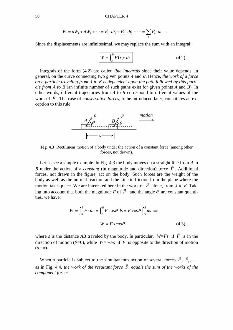
50 CHAPTER 4
1 2 1 1 2 2 i ii
W dW dW F dr F dr F dr= + + = ⋅ + ⋅ + = ⋅∑� � �� � �
⋯ ⋯ .
Since the displacements are infinitesimal, we may replace the sum with an integral:
( )B
AW F r dr= ⋅∫
� � �
(4.2)
Integrals of the form (4.2) are called line integrals since their value depends, in general, on the curve connecting two given points Α and Β. Hence, the work of a force on a particle traveling from Α to Β is dependent upon the path followed by this parti-cle from A to B (an infinite number of such paths exist for given points A and B). In other words, different trajectories from Α to Β correspond to different values of the work of F
�
. The case of conservative forces, to be introduced later, constitutes an ex-ception to this rule.
Fig. 4.3 Rectilinear motion of a body under the action of a constant force (among other forces, not drawn).
Let us see a simple example. In Fig. 4.3 the body moves on a straight line from Α to Β under the action of a constant (in magnitude and direction) force F
�
. Additional forces, not drawn in the figure, act on the body. Such forces are the weight of the body as well as the normal reaction and the kinetic friction from the plane where the motion takes place. We are interested here in the work of F
�
alone, from Α to Β. Tak-ing into account that both the magnitude F of F
�
, and the angle θ, are constant quanti-ties, we have:
cos cosB B B
A A AW F dr F ds F dsθ θ= ⋅ = = ⇒∫ ∫ ∫
� �
cosW F s θ= (4.3) where s is the distance AB traveled by the body. In particular, W=Fs if F
�
is in the direction of motion (θ=0), while W= −Fs if F
�
is opposite to the direction of motion (θ= π).
When a particle is subject to the simultaneous action of several forces 1 2, , ,F F� �
⋯
as in Fig. 4.4, the work of the resultant force F�
equals the sum of the works of the component forces.
F�
F�
θ θ
s
A Bmotion
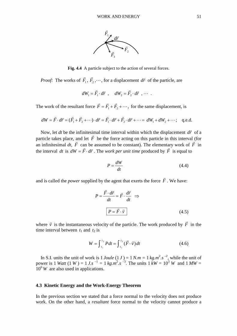
WORK AND ENERGY 51
1F�
2F�
3F�
dr�
Fig. 4.4 A particle subject to the action of several forces.
Proof: The works of 1 2, ,F F� �
⋯ , for a displacement dr�
of the particle, are
1 1 2 2, ,dW F dr dW F dr= ⋅ = ⋅
� �� �
⋯ .
The work of the resultant force 1 2F F F= + +
� � �
⋯ , for the same displacement, is
1 2 1 2 1 2( )dW F dr F F dr F dr F dr dW dW= ⋅ = + + ⋅ = ⋅ + ⋅ + = + +� � � � �� � � �
⋯ ⋯ ⋯ ; q.e.d.
Now, let dt be the infinitesimal time interval within which the displacement dr
�
of a particle takes place, and let F
�
be the force acting on this particle in this interval (for an infinitesimal dt, F
�
can be assumed to be constant). The elementary work of F�
in the interval dt is dW F dr= ⋅
� �
. The work per unit time produced by F�
is equal to
dW
Pdt
= (4.4)
and is called the power supplied by the agent that exerts the force F
�
. We have:
F dr dr
P Fdt dt
⋅= = ⋅ ⇒
� � ��
P F v= ⋅� �
(4.5) where v
�
is the instantaneous velocity of the particle. The work produced by F�
in the time interval between t1 and t2 is
2 2
1 1
( )t t
t tW Pdt F v dt= = ⋅∫ ∫
� �
(4.6)
In S.I. units the unit of work is 1 Joule (1 J ) = 1 N.m = 1 kg.m2.s –2, while the unit of power is 1 Watt (1 W ) = 1 J.s –1 = 1 kg.m2.s –3. The units 1 kW = 103 W and 1 MW = 106
W are also used in applications. 4.3 Kinetic Energy and the Work-Energy Theorem In the previous section we stated that a force normal to the velocity does not produce work. On the other hand, a resultant force normal to the velocity cannot produce a
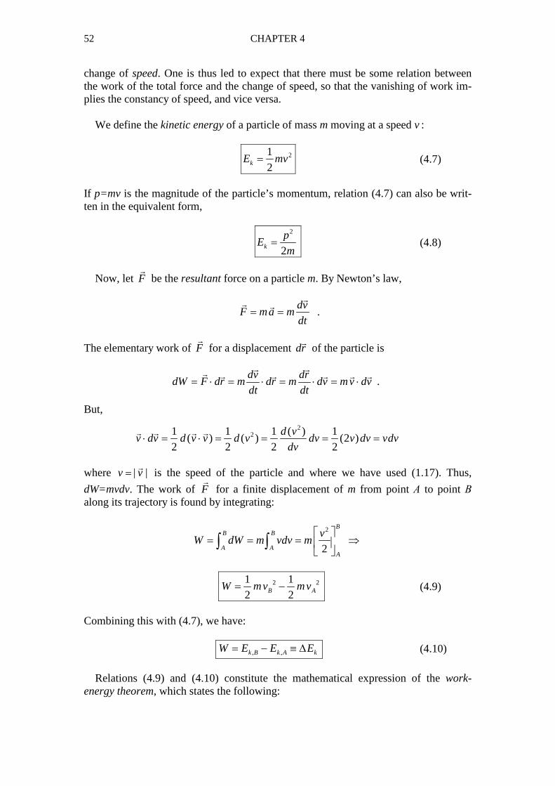
52 CHAPTER 4
change of speed. One is thus led to expect that there must be some relation between the work of the total force and the change of speed, so that the vanishing of work im-plies the constancy of speed, and vice versa. We define the kinetic energy of a particle of mass m moving at a speed v :
21
2kE mv= (4.7)
If p=mv is the magnitude of the particle’s momentum, relation (4.7) can also be writ-ten in the equivalent form,
2
2k
pE
m= (4.8)
Now, let F
�
be the resultant force on a particle m. By Newton’s law,
dv
F ma mdt
= =�
� �
.
The elementary work of F
�
for a displacement dr�
of the particle is
dv dr
dW F dr m dr m dv mv dvdt dt
= ⋅ = ⋅ = ⋅ = ⋅� �
� � � � � �
.
But,
2
21 1 1 ( ) 1( ) ( ) (2 )
2 2 2 2
d vv dv d v v d v dv v dv vdv
dv⋅ = ⋅ = = = =� � � �
where | |v v=
�
is the speed of the particle and where we have used (1.17). Thus,
dW=mvdv. The work of F�
for a finite displacement of m from point Α to point Β along its trajectory is found by integrating:
2
2
BB B
A AA
vW dW m vdv m
= = = ⇒
∫ ∫
2 21 1
2 2B AW mv mv= − (4.9)
Combining this with (4.7), we have: , ,k B k A kW E E E= − ≡ ∆ (4.10)
Relations (4.9) and (4.10) constitute the mathematical expression of the work-energy theorem, which states the following:
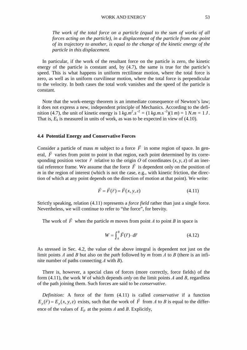
WORK AND ENERGY 53
The work of the total force on a particle (equal to the sum of works of all forces acting on the particle), in a displacement of the particle from one point of its trajectory to another, is equal to the change of the kinetic energy of the particle in this displacement.
In particular, if the work of the resultant force on the particle is zero, the kinetic energy of the particle is constant and, by (4.7), the same is true for the particle’s speed. This is what happens in uniform rectilinear motion, where the total force is zero, as well as in uniform curvilinear motion, where the total force is perpendicular to the velocity. In both cases the total work vanishes and the speed of the particle is constant. Note that the work-energy theorem is an immediate consequence of Newton’s law; it does not express a new, independent principle of Mechanics. According to the defi-nition (4.7), the unit of kinetic energy is 1 kg.m2.s -2 = (1 kg.m.s -2)(1 m) = 1 N.m = 1 J . That is, Ek is measured in units of work, as was to be expected in view of (4.10). 4.4 Potential Energy and Conservative Forces Consider a particle of mass m subject to a force F
�
in some region of space. In gen-eral, F
�
varies from point to point in that region, each point determined by its corre-sponding position vector r
�
relative to the origin Ο of coordinates (x, y, z) of an iner-tial reference frame. We assume that the force F
�
is dependent only on the position of m in the region of interest (which is not the case, e.g., with kinetic friction, the direc-tion of which at any point depends on the direction of motion at that point). We write: ( ) ( , , )F F r F x y z= =
� � ��
(4.11) Strictly speaking, relation (4.11) represents a force field rather than just a single force. Nevertheless, we will continue to refer to “the force”, for brevity. The work of F
�
when the particle m moves from point Α to point Β in space is
( )B
AW F r dr= ⋅∫
� � �
(4.12)
As stressed in Sec. 4.2, the value of the above integral is dependent not just on the limit points Α and Β but also on the path followed by m from Α to Β (there is an infi-nite number of paths connecting Α with Β). There is, however, a special class of forces (more correctly, force fields) of the form (4.11), the work W of which depends only on the limit points Α and Β, regardless of the path joining them. Such forces are said to be conservative. Definition: A force of the form (4.11) is called conservative if a function
( ) ( , , )p pE r E x y z=�
exists, such that the work of F�
from Α to Β is equal to the differ-
ence of the values of Ep at the points Α and Β. Explicitly,
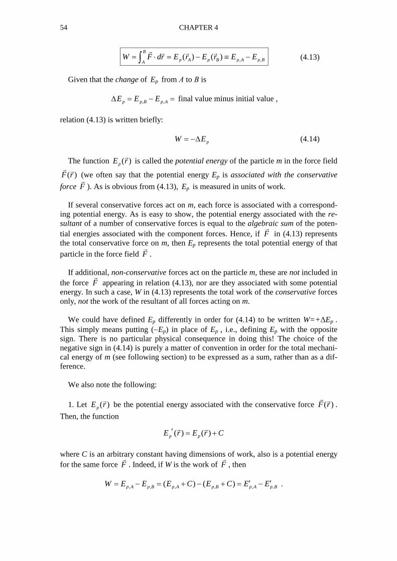
54 CHAPTER 4
, ,( ) ( )B
p A p B p A p BAW F dr E r E r E E= ⋅ = − ≡ −∫
� � � �
(4.13)
Given that the change of Ep from Α to Β is , ,p p B p AE E E∆ = − = final value minus initial value ,
relation (4.13) is written briefly: pW E= −∆ (4.14)
The function ( )pE r
�
is called the potential energy of the particle m in the force field
( )F r� �
(we often say that the potential energy Ep is associated with the conservative
force F�
). As is obvious from (4.13), Ep is measured in units of work. If several conservative forces act on m, each force is associated with a correspond-ing potential energy. As is easy to show, the potential energy associated with the re-sultant of a number of conservative forces is equal to the algebraic sum of the poten-tial energies associated with the component forces. Hence, if F
�
in (4.13) represents the total conservative force on m, then Ep represents the total potential energy of that particle in the force field F
�
. If additional, non-conservative forces act on the particle m, these are not included in the force F
�
appearing in relation (4.13), nor are they associated with some potential energy. In such a case, W in (4.13) represents the total work of the conservative forces only, not the work of the resultant of all forces acting on m. We could have defined Ep differently in order for (4.14) to be written W=+∆Ep . This simply means putting (−Ep) in place of Ep , i.e., defining Ep with the opposite sign. There is no particular physical consequence in doing this! The choice of the negative sign in (4.14) is purely a matter of convention in order for the total mechani-cal energy of m (see following section) to be expressed as a sum, rather than as a dif-ference. We also note the following: 1. Let ( )pE r
�
be the potential energy associated with the conservative force ( )F r� �
.
Then, the function
( ) ( )p pE r E r C′ = +� �
where C is an arbitrary constant having dimensions of work, also is a potential energy for the same force F
�
. Indeed, if W is the work of F�
, then , , , , , ,( ) ( )p A p B p A p B p A p BW E E E C E C E E′ ′= − = + − + = − .
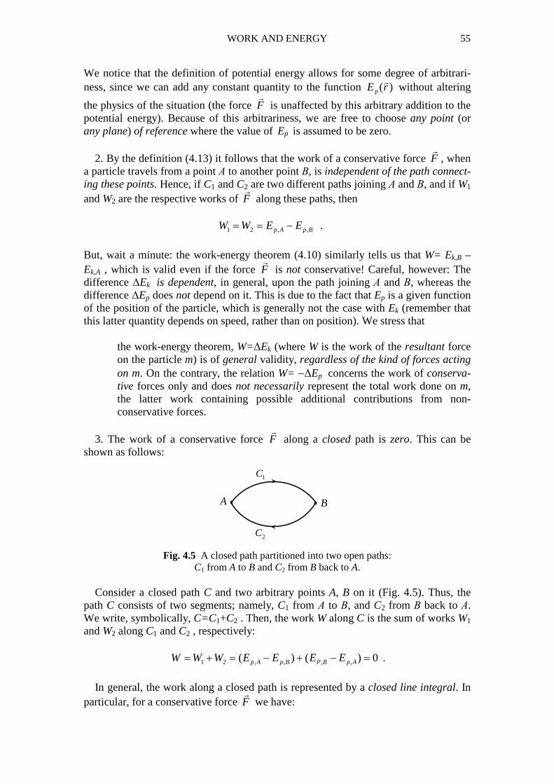
WORK AND ENERGY 55
We notice that the definition of potential energy allows for some degree of arbitrari-ness, since we can add any constant quantity to the function ( )pE r
�
without altering
the physics of the situation (the force F�
is unaffected by this arbitrary addition to the potential energy). Because of this arbitrariness, we are free to choose any point (or any plane) of reference where the value of Ep is assumed to be zero. 2. By the definition (4.13) it follows that the work of a conservative force F
�
, when a particle travels from a point Α to another point Β, is independent of the path connect-ing these points. Hence, if C1 and C2 are two different paths joining Α and Β, and if W1 and W2 are the respective works of F
�
along these paths, then 1 2 , ,p A p BW W E E= = − .
But, wait a minute: the work-energy theorem (4.10) similarly tells us that W= Ek,B –Ek,A , which is valid even if the force F
�
is not conservative! Careful, however: The difference ∆Ek is dependent, in general, upon the path joining Α and Β, whereas the difference ∆Ep does not depend on it. This is due to the fact that Ep is a given function of the position of the particle, which is generally not the case with Ek (remember that this latter quantity depends on speed, rather than on position). We stress that
the work-energy theorem, W=∆Ek (where W is the work of the resultant force on the particle m) is of general validity, regardless of the kind of forces acting on m. On the contrary, the relation W= −∆Ep concerns the work of conserva-tive forces only and does not necessarily represent the total work done on m, the latter work containing possible additional contributions from non-conservative forces.
3. The work of a conservative force F�
along a closed path is zero. This can be shown as follows:
A B
1C
2C
Fig. 4.5 A closed path partitioned into two open paths: C1 from A to B and C2 from B back to A.
Consider a closed path C and two arbitrary points A, B on it (Fig. 4.5). Thus, the path C consists of two segments; namely, C1 from Α to Β, and C2 from Β back to Α. We write, symbolically, C=C1+C2 . Then, the work W along C is the sum of works W1 and W2 along C1 and C2 , respectively: 1 2 , , , ,( ) ( ) 0p A p B P B p AW W W E E E E= + = − + − = .
In general, the work along a closed path is represented by a closed line integral. In particular, for a conservative force F
�
we have:
56 CHAPTER 4
0W F dr= ⋅ =∫� �
�
where the little circle on the integral sign indicates that the path of integration is a closed curve. We remark that the above-stated properties of conservative forces may in fact be regarded as definitions of the concept of a conservative force, equivalent to (4.13) (see, e.g., [1]). 4.5 Conservation of Mechanical Energy Consider a particle of mass m moving from point Α to point Β in some region of space, under the action of a force (more correctly, a force field) F
� which is the resul-
tant of all forces acting on m. According to the work-energy theorem, the work W of F�
equals the change of kinetic energy of m : , ,k k B k AW E E E= ∆ = − (4.15)
We stress again that (4.15) gives the work of the resultant force, regardless of whether this force is conservative or not. Now, if it happens that the total force F
� is conserva-
tive (which means that all component forces on m are conservative) then the work of F�
can be expressed as , ,p p A p BW E E E= −∆ = − (4.16)
where Ep is the total potential energy of m. Equating the right-hand sides of (4.15) and (4.16), we have: , , , ,k A p A k B p BE E E E+ = + (4.17)
Relation (4.17) is valid for any two points Α and Β between which the motion of m takes place. We thus conclude that the quantity
21( )
2k p pE E E mv E r= + = +�
(4.18)
which is called the total mechanical energy of m in the force field F
�, is constant dur-
ing the motion of m in that field. The above conclusion leads us to the principle of conservation of mechanical en-ergy:
If all forces acting on a particle m are conservative, the total mechanical en-ergy of m retains a constant value along the particle’s trajectory.
WORK AND ENERGY 57
We now see the logic behind the term “conservative force”. For non-conservative forces (such as, e.g., kinetic friction; see Sec. 4.7) it is not possible to define a poten-tial energy, thus also a total mechanical energy. Conservation of mechanical energy must therefore be reexamined when such forces are present. So, how do we handle the case where a particle m is subject to the simultaneous action of both conservative and non-conservative forces (such as, e.g., gravity and air resistance, respectively, for a falling body)? Let F
�
be the total conservative force on m, and let F ′
�
be the total non-conservative force on this particle. The resultant of all forces on m is
totF F F ′= +� � �
and the work of this force from Α to Β is
B B B
totA A AW F dr F dr F dr′= ⋅ = ⋅ + ⋅∫ ∫ ∫
� � �� � �
(4.19)
The first integral on the right is equal to the difference (Ep,A – Ep,B), where Ep is the potential energy associated with the conservative force F
�
, while the second integral represents the work W′ of the non-conservative force F ′
�
. Furthermore, by the work-
energy theorem, the work W of the resultant force totF�
is equal to (Ek,B – Ek,A). Relation
(4.19) is thus written as , , , ,( )k B k A p A p BE E E E W′− = − + ⇒
, , , ,( ) ( ) ( )k B p B k A p A k pW E E E E E E′ = + − + ≡ ∆ + (4.20)
We therefore conclude that
if non-conservative forces are present, the sum (Ek+Ep) is not constant, in general; specifically, this quantity changes by an amount equal to the work of the non-conservative forces.
An exception occurs when the non-conservative forces do not produce work, i.e., when 0W′ = . This is the case when the total non-conservative force F ′
�
is normal to the velocity of m. It then follows from (4.20) that the sum (Ek+Ep) is constant: ( ) 0k p k pE E E E∆ + = ⇔ + = constant, when 0W′ = .
We may thus express the principle of conservation of mechanical energy more gen-erally, as follows:
If the non-conservative forces that act on a particle do not produce work, the total mechanical energy of the particle is constant.

58 CHAPTER 4
For example, we apply conservation of mechanical energy in the study of the motion of a pendulum (see Problem 25) despite the fact that the bob of the pendulum is sub-ject not only to the conservative force of gravity but also to the tension of the string. This tension does not produce work, however, since it is always perpendicular to the velocity of the bob (explain why). Note: Equation (4.20) may be interpreted more generally, as follows: Assume that the total force acting on a particle can be written as a sum of two forces, F
�
and F ′�
, where F
�
is conservative and is associated with some potential energy Ep , while F ′�
may be of any kind, i.e., conservative, non-conservative, or with mixed conservative
and non-conservative components. Then, according to (4.20), the work W′ of F ′�
equals the change of the sum (Ek+Ep) . 4.6 Examples of Conservative Forces The following examples demonstrate a method for showing that a given force field is conservative. Specifically, we evaluate the work W of the force for an arbitrary path from A to B and then use equation (4.13) to read off the potential energy Ep , if it ex-ists. The existence of Ep automatically proves the conservative property of the given force field. 1. Force of gravity Near the surface of the Earth the acceleration g
�
of gravity is practically constant over large regions of space. Hence, in accordance with the results of Sec. 2.5, the mo-tion of a body under the sole action of gravity takes place in a constant plane – say, the xy-plane – perpendicular to the surface of the Earth, where the x-axis is horizontal while the y-axis is vertical and, by arbitrary choice, directed upward (see Fig. 4.6).
The y-coordinate specifies the instantaneous height at which a particle is located above an arbitrary horizontal reference level at which y=0. With the chosen upward direction of the vertical axis, the particle is above or below the reference level if y>0 or y<0, respectively. In a 3-dimensional Cartesian coordinate system (x, y, z) the z-coordinate of the particle has the fixed value z=0, where the z-axis (not shown in Fig. 4.6) is normal to the page and directed toward the reader.
O
ˆxu
ˆ yu
x
y
A
Bm
mg�
dr�
g�
B Ay y−
reference level
Fig. 4.6 Motion of a body near the surface of the Earth, under the sole action of gravity.
WORK AND ENERGY 59
The weight of a particle of mass m is a force perpendicular to the surface of the Earth (thus parallel to the y-axis) and directed downward:
ˆ (0, , 0)yF mg mgu mg= = − ≡ −� �
(the x- and z-components of F
�
are zero). On the other hand, an elementary displace-ment in space is written, in general, ˆ ˆ ˆ ˆ ˆ ˆ( ) ( ) ( ) ( ) ( , , )x y z x y zdr d xu yu zu dx u dy u dz u dx dy dz= + + = + + ≡
�
.
Here z is fixed, so that dz=0. Thus, an elementary displacement of the particle on its trajectory is written: ˆ ˆ( ) ( ) ( , , 0)x ydr dx u dy u dx dy= + ≡
�
.
Then, by using (1.19),
0 ( ) 0 0F dr dx mg dy mgdy⋅ = ⋅ + − + ⋅ = −� �
. The work of F
�
when m moves from Α to Β along its trajectory is
( )B B B
B AA A AW F dr mgdy mg dy mg y y= ⋅ = − = − = − − ⇒∫ ∫ ∫
� �
A BW mg y mg y= − (4.21)
Is the force F
�
conservative? In order for it to be, one should be able to find a func-tion ( )pE r
�
, the potential energy of m in the gravitational field of the Earth, such that
, ,p A p BW E E= − .
By (4.21) we see that such a function indeed exists: ( )pE y mgy= (4.22)
More generally, Ep=mgy+C , where C is an arbitrary constant quantity. We can elimi-nate C by (arbitrarily) requiring that Ep=0 at the reference level y=0. Exercise: Show that, if we choose the downward direction for the y-axis, then rela-tion (4.22) must be rewritten as Ep (y) = – mgy . According to the principle of conservation of mechanical energy, the total me-chanical energy of m remains fixed as the particle moves under the action of gravity (if we ignore non-conservative forces such as air resistance):
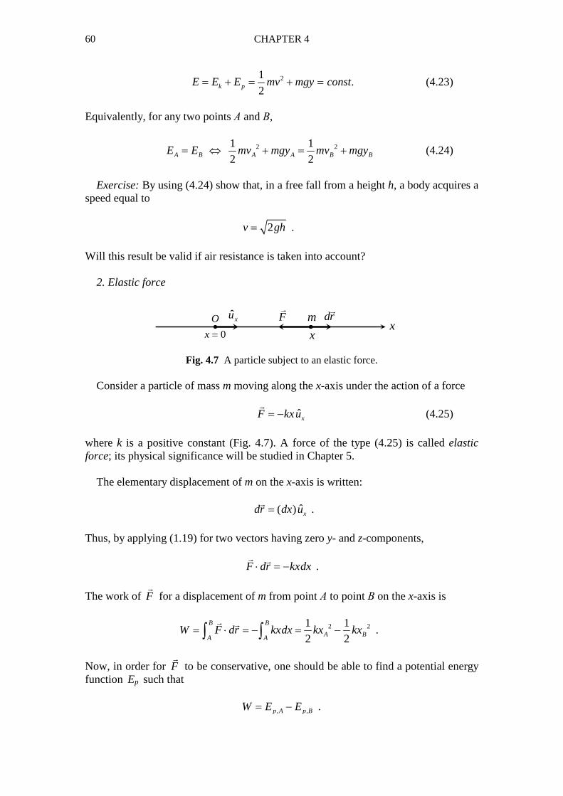
60 CHAPTER 4
21.
2k pE E E mv mgy const= + = + = (4.23)
Equivalently, for any two points Α and Β,
2 21 1
2 2A B A A B BE E mv mgy mv mgy= ⇔ + = + (4.24)
Exercise: By using (4.24) show that, in a free fall from a height h, a body acquires a speed equal to
2v gh= . Will this result be valid if air resistance is taken into account? 2. Elastic force
Fig. 4.7 A particle subject to an elastic force. Consider a particle of mass m moving along the x-axis under the action of a force ˆxF kxu= −
�
(4.25)
where k is a positive constant (Fig. 4.7). A force of the type (4.25) is called elastic force; its physical significance will be studied in Chapter 5. The elementary displacement of m on the x-axis is written: ˆ( ) xdr dx u=
�
.
Thus, by applying (1.19) for two vectors having zero y- and z-components, F dr kxdx⋅ = −
� �
. The work of F
�
for a displacement of m from point Α to point Β on the x-axis is
2 21 1
2 2
B B
A BA AW F dr kxdx kx kx= ⋅ = − = −∫ ∫
� �
.
Now, in order for F
�
to be conservative, one should be able to find a potential energy function Ep such that , ,p A p BW E E= − .
0
O
x = xx
ˆxu mF�
dr�
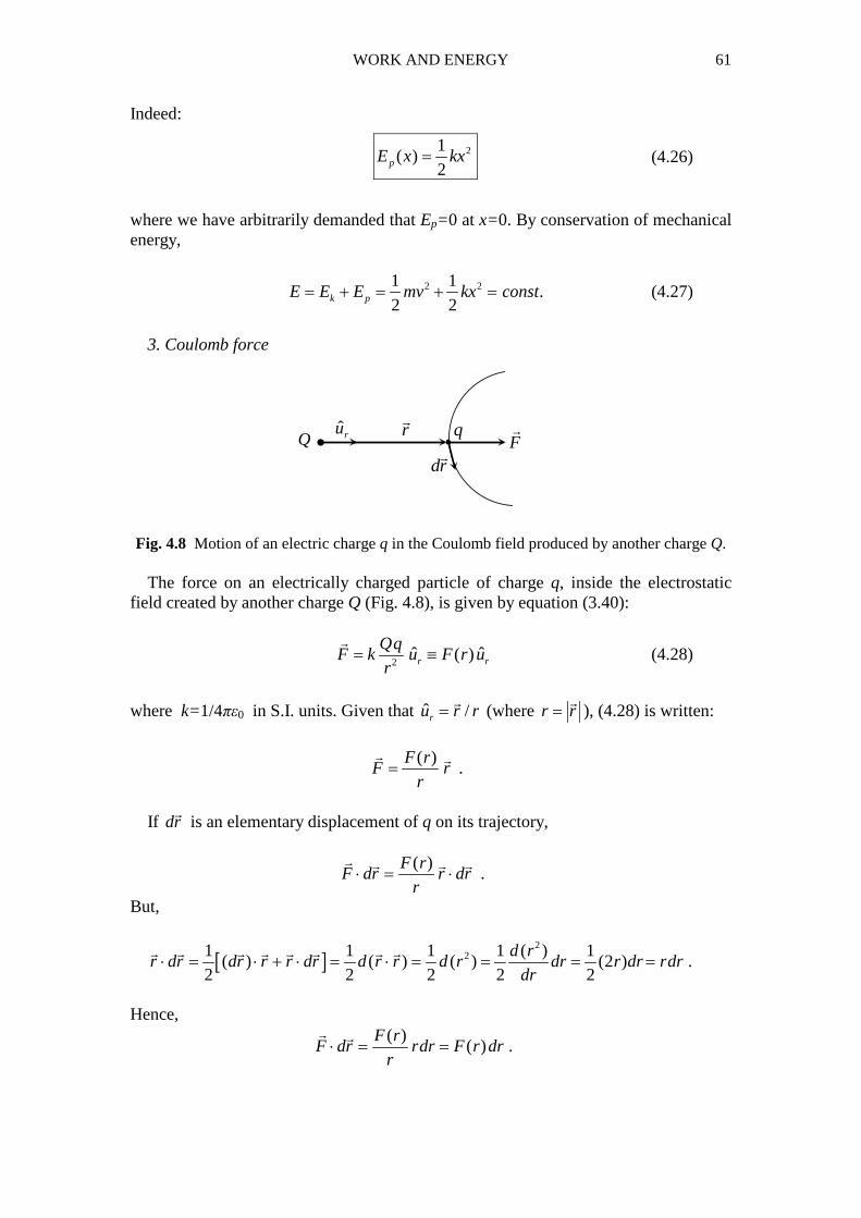
WORK AND ENERGY 61
Indeed:
21( )
2pE x kx= (4.26)
where we have arbitrarily demanded that Ep=0 at x=0. By conservation of mechanical energy,
2 21 1.
2 2k pE E E mv kx const= + = + = (4.27)
3. Coulomb force Fig. 4.8 Motion of an electric charge q in the Coulomb field produced by another charge Q.
The force on an electrically charged particle of charge q, inside the electrostatic field created by another charge Q (Fig. 4.8), is given by equation (3.40):
2
ˆ ˆ( )r r
QqF k u F r u
r= ≡�
(4.28)
where k=1/4πε0 in S.I. units. Given that /ru r r=
�
(where r r=�
), (4.28) is written:
( )F r
F rr
=� �
.
If dr
�
is an elementary displacement of q on its trajectory,
( )F r
F dr r drr
⋅ = ⋅� � � �
.
But,
[ ]2
21 1 1 1 ( ) 1( ) ( ) ( ) (2 ) .
2 2 2 2 2
d rr dr dr r r dr d r r d r dr r dr rdr
dr⋅ = ⋅ + ⋅ = ⋅ = = = =� � � � � � � �
Hence,
( )
( ) .F r
F dr rdr F r drr
⋅ = =� �
•Qˆru r
�
q
dr�
F�
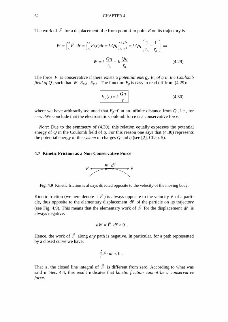
62 CHAPTER 4
The work of F�
for a displacement of q from point Α to point Β on its trajectory is
2
1 1( )
B B B
A A AA B
drW F dr F r dr k Qq k Qq
r r r
= ⋅ = = = − ⇒
∫ ∫ ∫� �
A B
Qq QqW k k
r r= − (4.29)
The force F
�
is conservative if there exists a potential energy Ep of q in the Coulomb field of Q , such that W=Ep,A –Ep,B . The function Ep is easy to read off from (4.29):
( )p
QqE r k
r= (4.30)
where we have arbitrarily assumed that Ep=0 at an infinite distance from Q , i.e., for r=∞. We conclude that the electrostatic Coulomb force is a conservative force. Note: Due to the symmetry of (4.30), this relation equally expresses the potential energy of Q in the Coulomb field of q. For this reason one says that (4.30) represents the potential energy of the system of charges Q and q (see [2], Chap. 5). 4.7 Kinetic Friction as a Non-Conservative Force
•m dr�
v�
F�
Fig. 4.9 Kinetic friction is always directed opposite to the velocity of the moving body. Kinetic friction (we here denote it F
�
) is always opposite to the velocity v�
of a parti-cle, thus opposite to the elementary displacement dr
�
of the particle on its trajectory (see Fig. 4.9). This means that the elementary work of F
�
for the displacement dr�
is always negative: 0dW F dr= ⋅ <
� �
. Hence, the work of F
�
along any path is negative. In particular, for a path represented by a closed curve we have:
0F dr⋅ <∫� �
� .
That is, the closed line integral of F
� is different from zero. According to what was
said in Sec. 4.4, this result indicates that kinetic friction cannot be a conservative force.
WORK AND ENERGY 63
It is meaningless to ask whether static friction is or is not conservative, given that this force does not produce work (why?). In Chapter 7 we will see that we may use conservation of mechanical energy for rolling bodies in spite of the presence of static friction.
References
1. C.J. Papachristou, Aspects of Integrability of Differential Systems and Fields: A Mathematical Primer for Physicists (Springer, 2019)
2. C.J. Papachristou, Introduction to Electromagnetic Theory and the Physics of Conducting Solids (Springer, 2020)
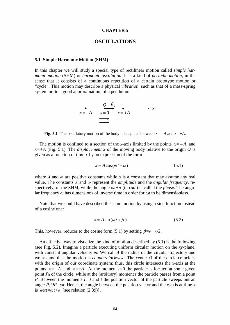
64
CHAPTER 5
OSCILLATIONS 5.1 Simple Harmonic Motion (SHM) In this chapter we will study a special type of rectilinear motion called simple har-monic motion (SHM) or harmonic oscillation. It is a kind of periodic motion, in the sense that it consists of a continuous repetition of a certain prototype motion or “cycle”. This motion may describe a physical vibration, such as that of a mass-spring system or, to a good approximation, of a pendulum.
Fig. 5.1 The oscillatory motion of the body takes place between x= –A and x=+A.
The motion is confined to a section of the x-axis limited by the points x= – A and x=+A (Fig. 5.1). The displacement x of the moving body relative to the origin O is given as a function of time t by an expression of the form cos( )x A tω α= + (5.1) where Α and ω are positive constants while α is a constant that may assume any real value. The constants Α and ω represent the amplitude and the angular frequency, re-spectively, of the SHM, while the angle ωt+α (in rad ) is called the phase. The angu-lar frequency ω has dimensions of inverse time in order for ωt to be dimensionless. Note that we could have described the same motion by using a sine function instead of a cosine one: sin ( )x A tω β= + (5.2) This, however, reduces to the cosine form (5.1) by setting β=α+π/2 . An effective way to visualize the kind of motion described by (5.1) is the following (see Fig. 5.2). Imagine a particle executing uniform circular motion on the xy-plane, with constant angular velocity ω. We call Α the radius of the circular trajectory and we assume that the motion is counterclockwise. The center Ο of the circle coincides with the origin of our coordinate system; thus, this circle intersects the x-axis at the points x= −A and x=+A . At the moment t=0 the particle is located at some given point Ρ0 of the circle, while at the (arbitrary) moment t the particle passes from a point Ρ. Between the moments t=0 and t the position vector of the particle sweeps out an angle Ρ0ΟΡ=ωt. Hence, the angle between the position vector and the x-axis at time t is φ(t)=ωt+α [see relation (2.39)] .
• •O
xˆxu
x A= − x A=+0x=
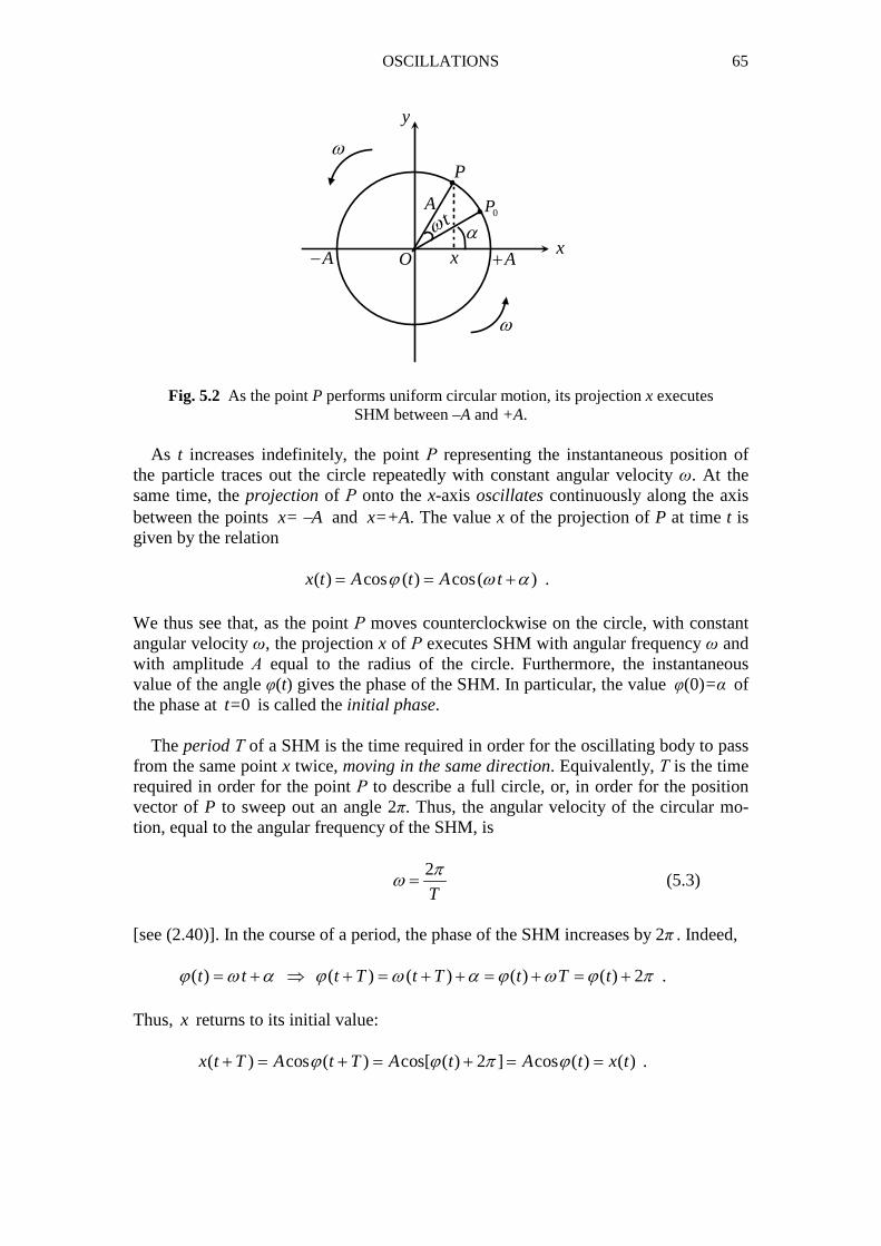
OSCILLATIONS 65
x
y
A− A+O
ω
ω
0P
P
A
xα
tω
Fig. 5.2 As the point P performs uniform circular motion, its projection x executes SHM between –A and +A.
As t increases indefinitely, the point Ρ representing the instantaneous position of the particle traces out the circle repeatedly with constant angular velocity ω. At the same time, the projection of Ρ onto the x-axis oscillates continuously along the axis between the points x= −A and x=+A. The value x of the projection of P at time t is given by the relation ( ) cos ( ) cos( )x t A t A tϕ ω α= = + . We thus see that, as the point Ρ moves counterclockwise on the circle, with constant angular velocity ω, the projection x of Ρ executes SHM with angular frequency ω and with amplitude Α equal to the radius of the circle. Furthermore, the instantaneous value of the angle φ(t) gives the phase of the SHM. In particular, the value φ(0)=α of the phase at t=0 is called the initial phase. The period Τ of a SHM is the time required in order for the oscillating body to pass from the same point x twice, moving in the same direction. Equivalently, Τ is the time required in order for the point Ρ to describe a full circle, or, in order for the position vector of P to sweep out an angle 2π. Thus, the angular velocity of the circular mo-tion, equal to the angular frequency of the SHM, is
2
T
πω = (5.3)
[see (2.40)]. In the course of a period, the phase of the SHM increases by 2π . Indeed, ( ) ( ) ( ) ( ) ( ) 2t t t T t T t T tϕ ω α ϕ ω α ϕ ω ϕ π= + ⇒ + = + + = + = + . Thus, x returns to its initial value: ( ) cos ( ) cos[ ( ) 2 ] cos ( ) ( )x t T A t T A t A t x tϕ ϕ π ϕ+ = + = + = = .
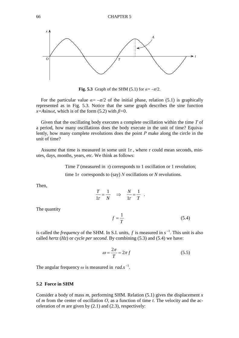
66 CHAPTER 5
Ot
x
A
T
Fig. 5.3 Graph of the SHM (5.1) for α= –π/2. For the particular value α= –π/2 of the initial phase, relation (5.1) is graphically represented as in Fig. 5.3. Notice that the same graph describes the sine function
x=Asinωt, which is of the form (5.2) with β=0. Given that the oscillating body executes a complete oscillation within the time Τ of a period, how many oscillations does the body execute in the unit of time? Equiva-lently, how many complete revolutions does the point Ρ make along the circle in the unit of time? Assume that time is measured in some unit 1τ , where τ could mean seconds, min-utes, days, months, years, etc. We think as follows:
Time Τ (measured in τ) corresponds to 1 oscillation or 1 revolution;
time 1τ corresponds to (say) Ν oscillations or N revolutions. Then,
1 1
1 1
T N
N Tτ τ= ⇒ = .
The quantity
1
fT
= (5.4)
is called the frequency of the SHM. In S.I. units, f is measured in s –1. This unit is also called hertz (Hz) or cycle per second. By combining (5.3) and (5.4) we have:
2
2 fT
πω π= = (5.5)
The angular frequency ω is measured in rad.s –1. 5.2 Force in SHM Consider a body of mass m, performing SHM. Relation (5.1) gives the displacement x of m from the center of oscillation Ο, as a function of time t. The velocity and the ac-celeration of m are given by (2.1) and (2.3), respectively:
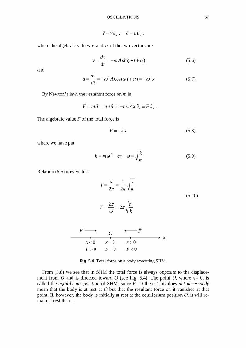
OSCILLATIONS 67
ˆ ˆ,x xv vu a au= =� �
,
where the algebraic values v and a of the two vectors are
sin( )dx
v A tdt
ω ω α= = − + (5.6)
and
2 2cos( )dv
a A t xdt
ω ω α ω= = − + = − (5.7)
By Newton’s law, the resultant force on m is 2ˆ ˆ ˆx x xF ma mau m x u F uω= = = − ≡
� �
.
The algebraic value F of the total force is F k x= − (5.8) where we have put
2 kk m
mω ω= ⇔ = (5.9)
Relation (5.5) now yields:
1
2 2
22
kf
m
mT
k
ωπ π
ππ
ω
= =
= =
(5.10)
i ii
OF�
F�
0
0
x
F
=
=
0
0
x
F
<
>
0
0
x
F
>
<
x
Fig. 5.4 Total force on a body executing SHM. From (5.8) we see that in SHM the total force is always opposite to the displace-ment from Ο and is directed toward Ο (see Fig. 5.4). The point Ο, where x= 0, is called the equilibrium position of SHM, since F= 0 there. This does not necessarily mean that the body is at rest at Ο but that the resultant force on it vanishes at that point. If, however, the body is initially at rest at the equilibrium position Ο, it will re-main at rest there.
68 CHAPTER 5
5.3 Energy Relations With the aid of (5.6) we can find an expression for the kinetic energy of a body of mass m, executing SHM:
2 2 2 2 2 2 2 21 1 1sin ( ) [ cos ( )]
2 2 2kE mv m A t m A A tω ω α ω ω α= = + = − + .
By using (5.1) and (5.9) we get:
2 21( )
2kE k A x= − (5.11)
We notice that Ek obtains its maximum value at the equilibrium position (x=0) and vanishes at the extreme points (x=±A) of the oscillation. It follows from (5.8) that the resultant force F
�
on the oscillating body is an elastic force of the form (4.25). As we showed in Sec. 4.6 [see relation (4.26)] the potential energy of the body is
21
2pE k x= (5.12)
We notice that Ep vanishes at the equilibrium position (x=0) while it obtains a maxi-mum value at the extreme points (x=±A) of the oscillation. From (5.11) and (5.12) we can find the total mechanical energy of the oscillating body:
21
2k pE E E k A= + = (5.13)
Notice that this quantity assumes a fixed value during the SHM, in accordance with the principle of conservation of mechanical energy. 5.4 Oscillations of a Mass-Spring System Springs are often used as instruments for producing SHM. Before we see how this is done, let us say a few words about the force a spring exerts on a body connected to it. The spring may be in one of the following three states:
1. In its natural length, which occurs when the spring is not subject to external forces. The spring then, in turn, does not exert a force on a body connected to it.
2. In extension by ∆l relative to its natural length. The spring then has a tendency to return to its natural length; it thus exerts a force kF
�
opposite to the extension, of mag-
nitude k∆l , where k is called the spring constant.
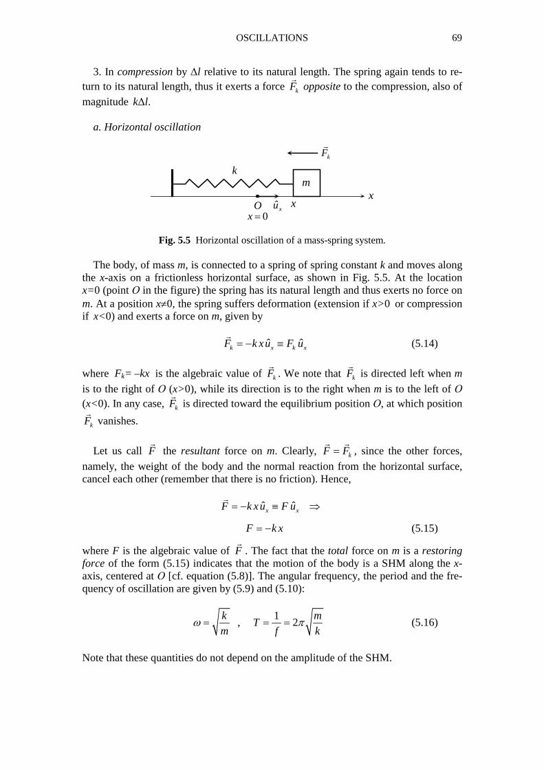
OSCILLATIONS 69
k
O0x=
xx
m
ˆxu
kF�
3. In compression by ∆l relative to its natural length. The spring again tends to re-turn to its natural length, thus it exerts a force kF
�
opposite to the compression, also of
magnitude k∆l. a. Horizontal oscillation
Fig. 5.5 Horizontal oscillation of a mass-spring system. The body, of mass m, is connected to a spring of spring constant k and moves along the x-axis on a frictionless horizontal surface, as shown in Fig. 5.5. At the location x=0 (point Ο in the figure) the spring has its natural length and thus exerts no force on m. At a position x≠0, the spring suffers deformation (extension if x>0 or compression if x<0) and exerts a force on m, given by ˆ ˆk x k xF k xu F u= − ≡
�
(5.14)
where Fk= –kx is the algebraic value of kF
�
. We note that kF�
is directed left when m
is to the right of Ο (x>0), while its direction is to the right when m is to the left of Ο (x<0). In any case, kF
�
is directed toward the equilibrium position Ο, at which position
kF�
vanishes.
Let us call F
�
the resultant force on m. Clearly, kF F=� �
, since the other forces,
namely, the weight of the body and the normal reaction from the horizontal surface, cancel each other (remember that there is no friction). Hence, ˆ ˆx xF k xu F u= − ≡ ⇒
�
F k x= − (5.15)
where F is the algebraic value of F�
. The fact that the total force on m is a restoring force of the form (5.15) indicates that the motion of the body is a SHM along the x-axis, centered at Ο [cf. equation (5.8)]. The angular frequency, the period and the fre-quency of oscillation are given by (5.9) and (5.10):
1
, 2k m
Tm f k
ω π= = = (5.16)
Note that these quantities do not depend on the amplitude of the SHM.
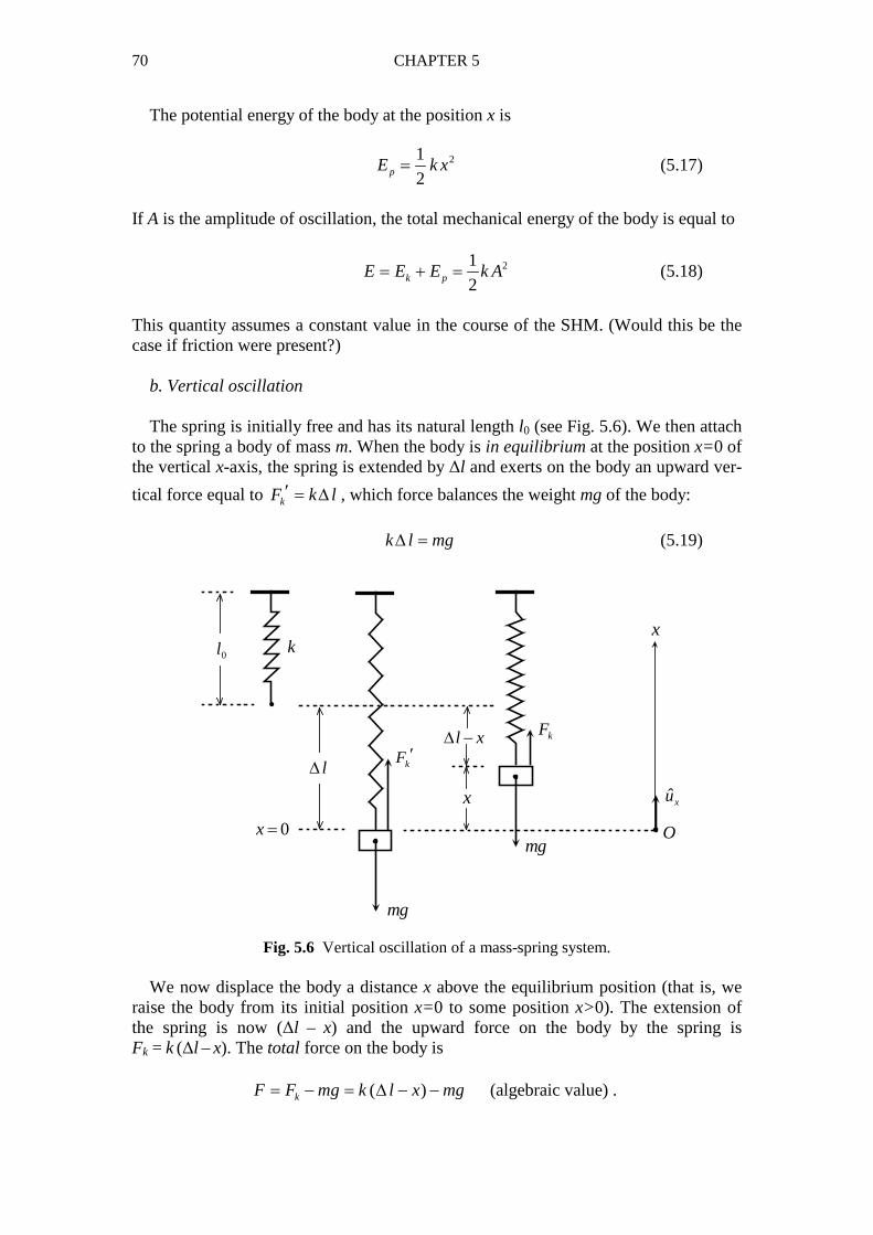
70 CHAPTER 5
i
0l k
l∆
0x=
mg
mg
l x∆ −
x
x
O
ˆxu
kF ′kF
The potential energy of the body at the position x is
21
2pE k x= (5.17)
If A is the amplitude of oscillation, the total mechanical energy of the body is equal to
21
2k pE E E k A= + = (5.18)
This quantity assumes a constant value in the course of the SHM. (Would this be the case if friction were present?) b. Vertical oscillation The spring is initially free and has its natural length l0 (see Fig. 5.6). We then attach to the spring a body of mass m. When the body is in equilibrium at the position x=0 of the vertical x-axis, the spring is extended by ∆l and exerts on the body an upward ver-
tical force equal to kF k l′ = ∆ , which force balances the weight mg of the body:
k l mg∆ = (5.19)
Fig. 5.6 Vertical oscillation of a mass-spring system. We now displace the body a distance x above the equilibrium position (that is, we raise the body from its initial position x=0 to some position x>0). The extension of the spring is now (∆l – x) and the upward force on the body by the spring is Fk = k (∆l – x). The total force on the body is ( )kF F mg k l x mg= − = ∆ − − (algebraic value) .
OSCILLATIONS 71
By making use of the equilibrium condition (5.19), we find: F k x= − (5.20) Equation (5.20) was derived for x>0, i.e., for a displacement of m above the equi-librium position. Consider now a displacement below the equilibrium position, at x<0. The extension of the spring is then ∆l + |x| = ∆l – x, as before, and our previous ex-pressions for the upward force Fk by the spring and for the total force F on m are still valid:
( ) ( ) ,
( )k
k
F k l x k l x
F F mg k l x mg k x
= ∆ + = ∆ −
= − = ∆ − − = −
where the equilibrium condition (5.19) was again used. In conclusion, the total force on the body is a restoring force of the form (5.20), where x is the displacement from the equilibrium position. Under the action of this force the body will execute SHM about its equilibrium position (at which position the extension of the spring is ∆l ). The angular frequency and the period of oscillation are
1
, 2k m
Tm f k
ω π= = = (5.21)
The potential energy of the body at a position x is
21
2pE k x= (5.22)
while the total mechanical energy of m is
21
2k pE E E k A= + = (5.23)
where Α is the amplitude of oscillation. We note again that Ε is a constant quantity. The force kF
�
exerted by a spring is conservative and is associated with a potential
energy , ( )p kE y , where y is the deformation (extension or compression) of the spring.
Indeed, this force is algebraically equal to
kF k y= −
where we assume that y>0 for extension and y<0 for compression. As in Example 2 of Sec. 4.6, the work of kF
�
for a displacement of the point of application of this force
from point Α to point Β is
2 2, ,
1 1( ) ( )
2 2
B B
k A B p k p kA AW F dr kydy ky ky E A E B= ⋅ = − = − ≡ −∫ ∫
� �
and therefore,
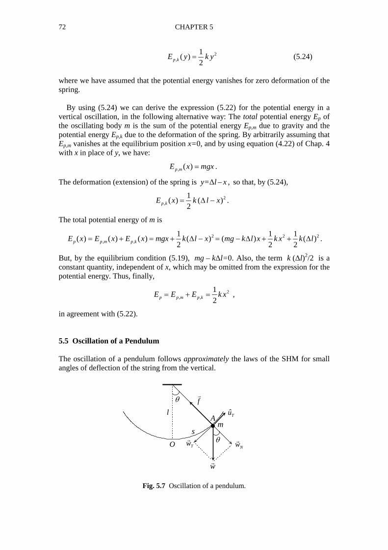
72 CHAPTER 5
2,
1( )
2p kE y k y= (5.24)
where we have assumed that the potential energy vanishes for zero deformation of the spring. By using (5.24) we can derive the expression (5.22) for the potential energy in a vertical oscillation, in the following alternative way: The total potential energy Ep of the oscillating body m is the sum of the potential energy Ep,m due to gravity and the potential energy Ep,k due to the deformation of the spring. By arbitrarily assuming that Ep,m vanishes at the equilibrium position x=0, and by using equation (4.22) of Chap. 4 with x in place of y, we have:
, ( )p mE x mgx= .
The deformation (extension) of the spring is y=∆l – x , so that, by (5.24),
2,
1( ) ( )
2p kE x k l x= ∆ − .
The total potential energy of m is
2 2 2, ,
1 1 1( ) ( ) ( ) ( ) ( ) ( )
2 2 2p p m p kE x E x E x mgx k l x mg k l x k x k l= + = + ∆ − = − ∆ + + ∆ .
But, by the equilibrium condition (5.19), mg – k∆l= 0. Also, the term k (∆l)2/2 is a constant quantity, independent of x, which may be omitted from the expression for the potential energy. Thus, finally,
2, ,
1
2p p m p kE E E k x= + = ,
in agreement with (5.22). 5.5 Oscillation of a Pendulum The oscillation of a pendulum follows approximately the laws of the SHM for small angles of deflection of the string from the vertical.
•
O
l
θ
θs
A
f�
w�
ˆTu
m
Tw�
Nw�
Fig. 5.7 Oscillation of a pendulum.
OSCILLATIONS 73
The mass m in Fig. 5.7 oscillates symmetrically about the equilibrium position Ο. For small angles θ of deflection, the arc ΟΑ may be approximated by a horizontal rectilinear segment of length s=lθ , where l is the length of the pendulum string and where θ is in rad. Here, s and θ represent the displacement from the equilibrium posi-tion. In particular, s>0 and θ>0 when m is to the right of Ο (in accordance with the positive direction of moving away from Ο, as defined by the unit tangent vector ˆTu )
while s<0 and θ<0 when m is to the left of Ο. The restoring force that is responsible for the oscillation is the tangential component of the total force on m, that is, the component parallel to the velocity of m. The mass m is subject to two forces; namely, the weight w
�
, of magnitude mg, and
the tension f�
of the string. The total force on m is F w f= +�� �
. As is easy to see, at
any point A the tangential component TF�
of F�
is equal to the tangential component
Tw�
of the weight:
ˆ ˆsinT T T T TF w mg u F uθ= = − ≡� �
where sinTF mg θ= − is the algebraic value of TF
�
. For sufficiently small values of
the angle θ, we can make the approximation sinθ θ≃ . Hence,
T
mgF mg s
lθ − = −
≃ (5.25)
(since s=lθ). Relation (5.25) is of the form (5.8), with s in place of x :
TF ks−≃ where mg
kl
= .
This means that, under the action of TF�
, the mass m executes SHM about the equilib-
rium position Ο. The angular frequency and the period of oscillation are
, 2 2k g m l
Tm l k g
ω π π= = = = (5.26)
Note that ω should not be interpreted as the angular velocity of the circular motion of m for finite values of θ and s. Indeed, since that motion is not uniform (why?) the corresponding angular velocity cannot be a constant, in contrast to the angular fre-quency ω in (5.26). 5.6 Differential Equation of SHM As defined in Sec. 5.1, SHM is a special kind of rectilinear motion in which the dis-placement x from the equilibrium position O is given as a function of time by equation (5.1). By Newton’s law, then, the total force on the oscillating body is a restoring force proportional to the displacement [see equation (5.8)].

74 CHAPTER 5
Conversely, let us assume that a particle of mass m is subject to a total force of the form (5.8): F= –kx. According to Newton’s law, this force is equal to F=ma, where
2
2
dv d dx d xa
dt dt dt dt
= = =
.
We thus have:
2 2
2 20
d x d x km kx x
mdt dt= − ⇔ + = .
Setting ω2=k/m [comp. equation (5.9)] we finally have:
2
22
0d x
xdt
ω+ = (5.27)
Relation (5.27) is a second-order differential equation for the function x=x(t). Its general solution must depend on two arbitrary constants (or parameters). As can be verified by direct substitution into (5.27), this solution is precisely the function cos( )x A tω α= + by which the SHM was defined in Sec. 5.1. The amplitude A and the initial phase α are the two parameters which the solution of (5.27) is required to contain. In the case of the pendulum (Sec. 5.5) the role of x is played by the arc s=lθ, which arc is almost rectilinear for small angles θ. Given that
2 2
2 2
d s dl
dt dt
θ= (since l is constant) ,
the differential equation (5.27) with s in place of x reduces to
2
22
0d
dt
θω θ+ = (5.28)
where ω2=g/l [see eq. (5.26)]. The general solution of (5.28) has the form 0 cos( )tθ θ ω α= + ,
where θ0 is the maximum angle of deflection of the string from the vertical. In the real world, oscillations are not as simple as those described by (5.27). Thus, in addition to a restoring force of the form (5.8) the body may be subject to a fric-tional force and/or an applied periodic force. These physical situations are referred to as damped oscillations and forced oscillations, accordingly [1-3] and are described mathematically by linear (homogeneous or non-homogeneous, as the case may be) differential equations of the second order [4].
OSCILLATIONS 75
References
1. K.R. Symon, Mechanics, 3rd Edition (Addison-Wesley, 1971)
2. J.B. Marion, S.T. Thornton, Classical Dynamics of Particles and Systems, 4th Edition (Saunders College, 1995)
3. J.R. Taylor, Classical Mechanics (University Science Books, 2005)
4. A.F. Bermant, I.G. Aramanovich, Mathematical Analysis (Mir Publishers, 1975)
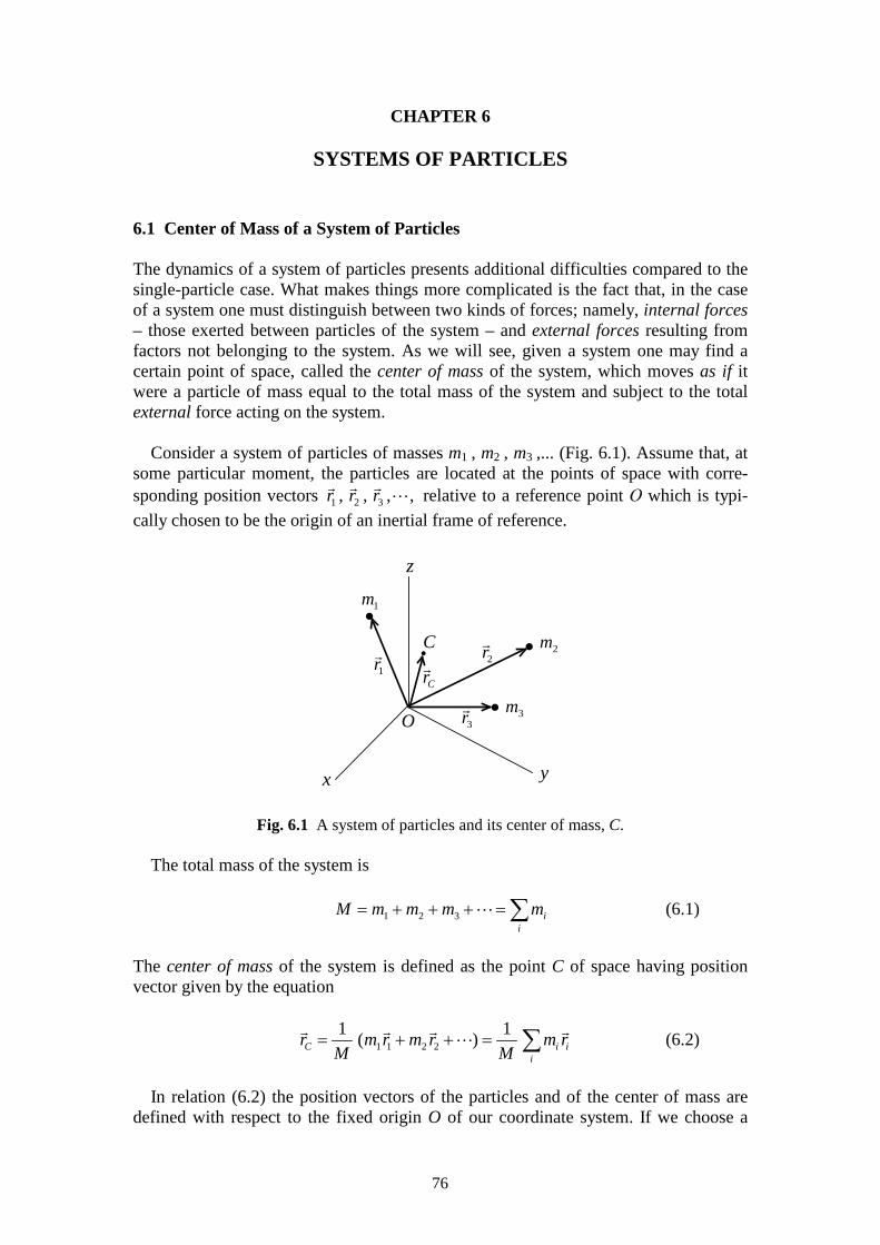
76
CHAPTER 6
SYSTEMS OF PARTICLES 6.1 Center of Mass of a System of Particles The dynamics of a system of particles presents additional difficulties compared to the single-particle case. What makes things more complicated is the fact that, in the case of a system one must distinguish between two kinds of forces; namely, internal forces – those exerted between particles of the system – and external forces resulting from factors not belonging to the system. As we will see, given a system one may find a certain point of space, called the center of mass of the system, which moves as if it were a particle of mass equal to the total mass of the system and subject to the total external force acting on the system. Consider a system of particles of masses m1 , m2 , m3 ,... (Fig. 6.1). Assume that, at some particular moment, the particles are located at the points of space with corre-sponding position vectors 1 2 3, , , ,r r r
� � �
⋯ relative to a reference point Ο which is typi-
cally chosen to be the origin of an inertial frame of reference.
Fig. 6.1 A system of particles and its center of mass, C.
The total mass of the system is 1 2 3 i
i
M m m m m= + + + =∑⋯ (6.1)
The center of mass of the system is defined as the point C of space having position vector given by the equation
1 1 2 2
1 1( )C i i
i
r m r m r m rM M
= + + = ∑� � � �
⋯ (6.2)
In relation (6.2) the position vectors of the particles and of the center of mass are defined with respect to the fixed origin O of our coordinate system. If we choose a
•
•
•
•
x y
z
O
1m
2m
3m
C
1r� 2r
�
3r�
Cr�
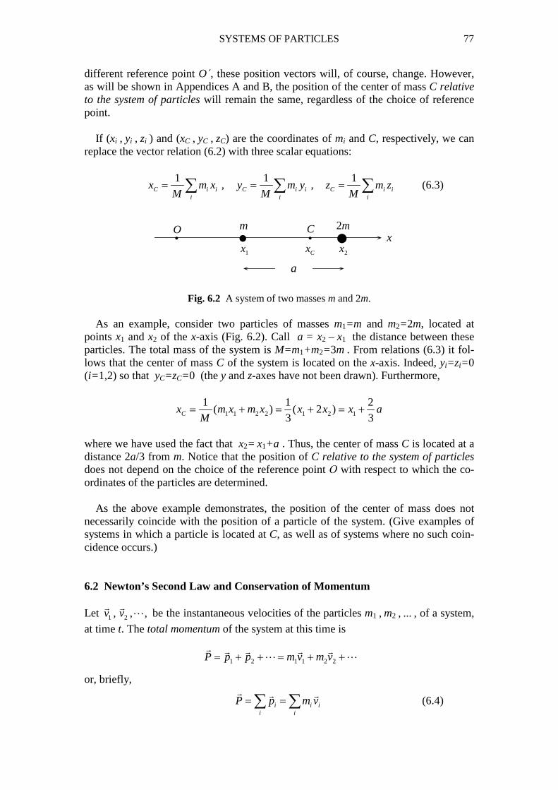
SYSTEMS OF PARTICLES 77
different reference point O΄, these position vectors will, of course, change. However, as will be shown in Appendices A and B, the position of the center of mass C relative to the system of particles will remain the same, regardless of the choice of reference point. If (xi , yi , zi ) and (xC , yC , zC) are the coordinates of mi and C, respectively, we can replace the vector relation (6.2) with three scalar equations:
1 1 1
, ,C i i C i i C i ii i i
x m x y m y z m zM M M
= = =∑ ∑ ∑ (6.3)
Fig. 6.2 A system of two masses m and 2m. As an example, consider two particles of masses m1=m and m2=2m, located at points x1 and x2 of the x-axis (Fig. 6.2). Call a = x2 – x1 the distance between these particles. The total mass of the system is M=m1+m2=3m . From relations (6.3) it fol-lows that the center of mass C of the system is located on the x-axis. Indeed, yi=zi=0 (i= 1,2) so that yC=zC=0 (the y and z-axes have not been drawn). Furthermore,
1 1 2 2 1 2 1
1 1 2( ) ( 2 )
3 3Cx m x m x x x x aM
= + = + = +
where we have used the fact that x2= x1+a . Thus, the center of mass C is located at a distance 2a/3 from m. Notice that the position of C relative to the system of particles does not depend on the choice of the reference point Ο with respect to which the co-ordinates of the particles are determined. As the above example demonstrates, the position of the center of mass does not necessarily coincide with the position of a particle of the system. (Give examples of systems in which a particle is located at C, as well as of systems where no such coin-cidence occurs.) 6.2 Newton’s Second Law and Conservation of Momentum Let 1 2, , ,v v� �
⋯ be the instantaneous velocities of the particles m1 , m2 , ... , of a system,
at time t. The total momentum of the system at this time is 1 2 1 1 2 2P p p m v m v= + + = + +
� � � � �
⋯ ⋯
or, briefly,
i i ii i
P p m v= =∑ ∑� � �
(6.4)
•• ••O C
xm 2m
1x 2xCx
a
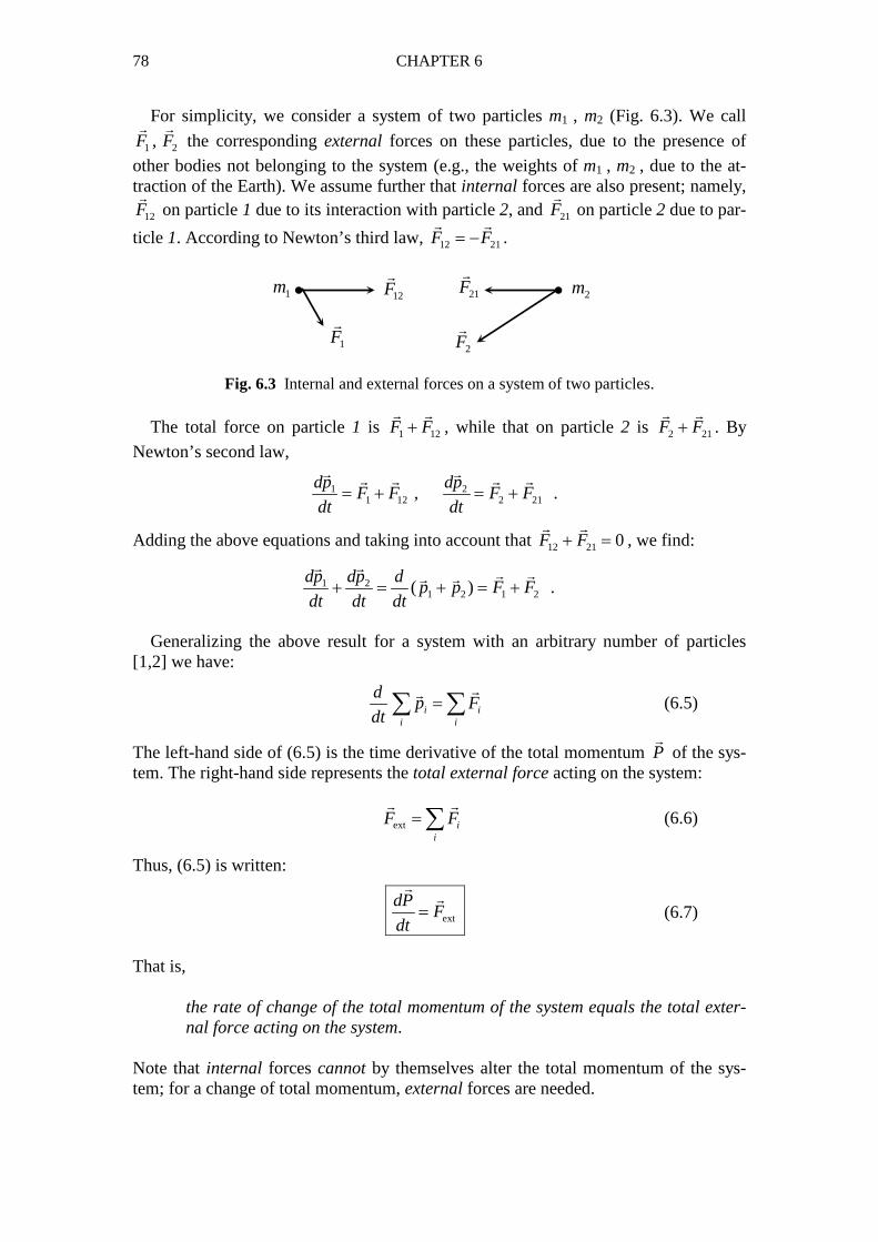
78 CHAPTER 6
For simplicity, we consider a system of two particles m1 , m2 (Fig. 6.3). We call
1 2,F F� �
the corresponding external forces on these particles, due to the presence of
other bodies not belonging to the system (e.g., the weights of m1 , m2 , due to the at-traction of the Earth). We assume further that internal forces are also present; namely,
12F�
on particle 1 due to its interaction with particle 2, and 21F�
on particle 2 due to par-
ticle 1. According to Newton’s third law, 12 21F F= −� �
.
Fig. 6.3 Internal and external forces on a system of two particles. The total force on particle 1 is 1 12F F+
� �
, while that on particle 2 is 2 21F F+� �
. By
Newton’s second law,
1 21 12 2 21,
dp dpF F F F
dt dt= + = +
� �� � � �
.
Adding the above equations and taking into account that 12 21 0F F+ =� �
, we find:
1 21 2 1 2( )
dp dp dp p F F
dt dt dt+ = + = +
� �� �� �
.
Generalizing the above result for a system with an arbitrary number of particles [1,2] we have:
i ii i
dp F
dt=∑ ∑
��
(6.5)
The left-hand side of (6.5) is the time derivative of the total momentum P�
of the sys-tem. The right-hand side represents the total external force acting on the system:
ext ii
F F=∑� �
(6.6)
Thus, (6.5) is written:
ext
dPF
dt=
�
�
(6.7)
That is,
the rate of change of the total momentum of the system equals the total exter-nal force acting on the system.
Note that internal forces cannot by themselves alter the total momentum of the sys-tem; for a change of total momentum, external forces are needed.
• •1m 2m
1F�
2F�
12F�
21F�
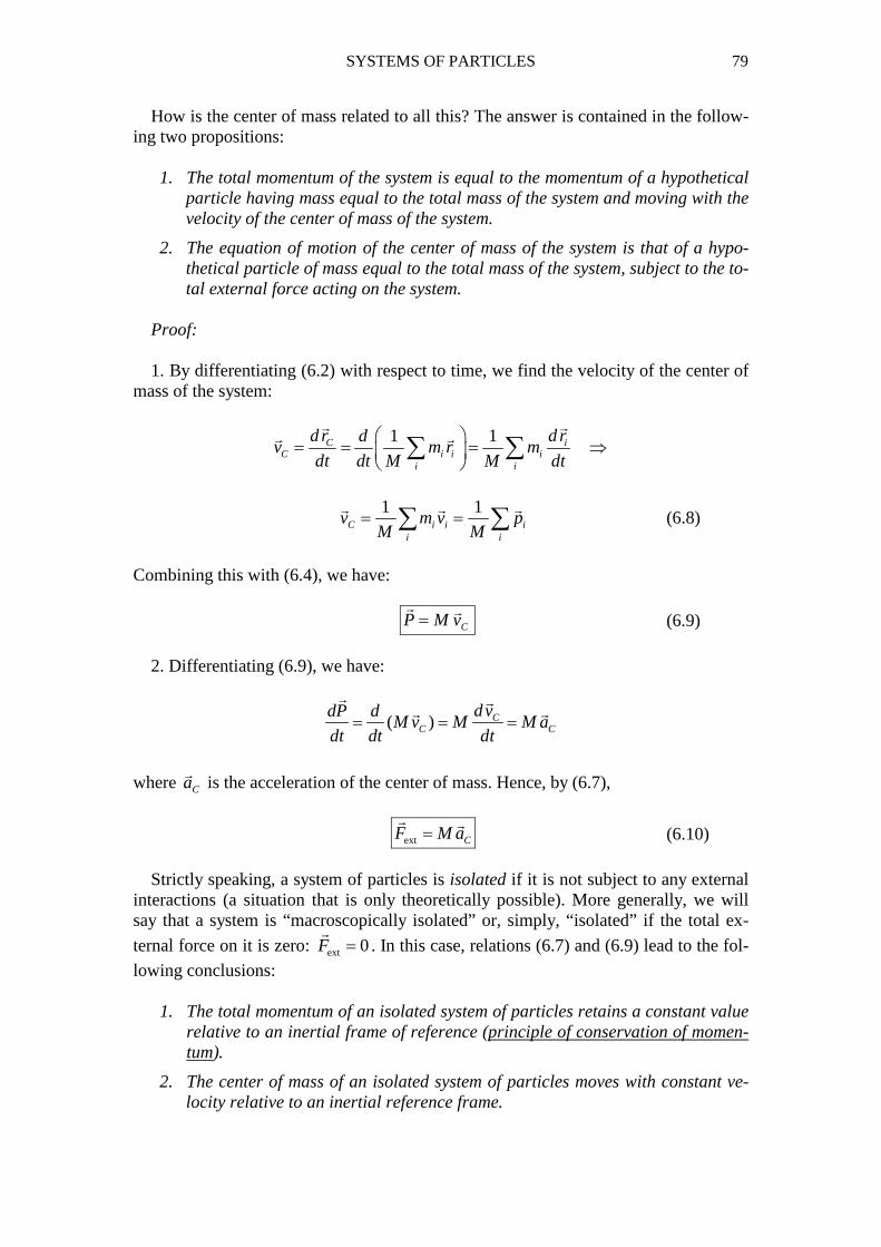
SYSTEMS OF PARTICLES 79
How is the center of mass related to all this? The answer is contained in the follow-ing two propositions:
1. The total momentum of the system is equal to the momentum of a hypothetical particle having mass equal to the total mass of the system and moving with the velocity of the center of mass of the system.
2. The equation of motion of the center of mass of the system is that of a hypo-thetical particle of mass equal to the total mass of the system, subject to the to-tal external force acting on the system.
Proof: 1. By differentiating (6.2) with respect to time, we find the velocity of the center of mass of the system:
1 1C iC i i i
i i
dr d rdv m r m
dt dt M M dt
= = = ⇒
∑ ∑
� �
� �
1 1
C i i ii i
v m v pM M
= =∑ ∑� � �
(6.8)
Combining this with (6.4), we have:
CP M v=� �
(6.9)
2. Differentiating (6.9), we have:
( ) CC C
dvdP dM v M M a
dt dt dt= = =
� �
� �
where Ca
�
is the acceleration of the center of mass. Hence, by (6.7),
ext CF M a=� �
(6.10)
Strictly speaking, a system of particles is isolated if it is not subject to any external interactions (a situation that is only theoretically possible). More generally, we will say that a system is “macroscopically isolated” or, simply, “isolated” if the total ex-
ternal force on it is zero: ext 0F =�
. In this case, relations (6.7) and (6.9) lead to the fol-
lowing conclusions:
1. The total momentum of an isolated system of particles retains a constant value relative to an inertial frame of reference (principle of conservation of momen-tum).
2. The center of mass of an isolated system of particles moves with constant ve-locity relative to an inertial reference frame.
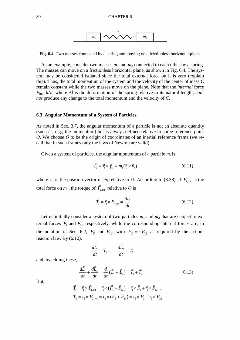
80 CHAPTER 6
1m 2mk
Fig. 6.4 Two masses connected by a spring and moving on a frictionless horizontal plane.
As an example, consider two masses m1 and m2 connected to each other by a spring. The masses can move on a frictionless horizontal plane, as shown in Fig. 6.4. The sys-tem may be considered isolated since the total external force on it is zero (explain this). Thus, the total momentum of the system and the velocity of the center of mass C remain constant while the two masses move on the plane. Note that the internal force Fint=k∆l, where ∆l is the deformation of the spring relative to its natural length, can-not produce any change to the total momentum and the velocity of C. 6.3 Angular Momentum of a System of Particles As noted in Sec. 3.7, the angular momentum of a particle is not an absolute quantity (such as, e.g., the momentum) but is always defined relative to some reference point Ο. We choose Ο to be the origin of coordinates of an inertial reference frame (we re-call that in such frames only the laws of Newton are valid). Given a system of particles, the angular momentum of a particle mi is ( )i i i i i iL r p m r v= × = ×
� � � � �
(6.11)
where ir�
is the position vector of mi relative to Ο. According to (3.38), if ,totiF�
is the
total force on mi , the torque of ,totiF�
relative to Ο is
,toti
i i i
dLT r F
dt= × =
�
� ��
(6.12)
Let us initially consider a system of two particles m1 and m2 that are subject to ex-
ternal forces 1 2andF F� �
, respectively, while the corresponding internal forces are, in
the notation of Sec. 6.2, 12 21andF F� �
, with 12 21F F= −� �
as required by the action-reaction law. By (6.12),
1 21 2,
dL dLT T
dt dt= =
� �
� �
and, by adding these,
1 21 2 1 2( )
dL dL dL L T T
dt dt dt+ = + = +
� �
� � � �
(6.13)
But,
1 1 1,tot 1 1 12 1 1 1 12
2 2 2,tot 2 2 21 2 2 2 21
( ) ,
( ) .
T r F r F F r F r F
T r F r F F r F r F
= × = × + = × + ×
= × = × + = × + ×
� � � � � �� � � �
� � � � � �� � � �
SYSTEMS OF PARTICLES 81
Adding the above equations and taking into account that 12 21F F= −� �
, we have:
1 2 1 1 2 2 1 2 12( )T T r F r F r r F+ = × + × + − ×� � � � �� � � �
.
The difference 1 2( )r r−� �
is a vector directed along the line joining the two particles (see
Sec. 1.3). If we make the additional assumption that the internal forces 12F�
and 21F�
act along this line, then
1 2 12( ) 0r r F− × =�� �
so that
1 2 1 1 2 2 extT T r F r F T+ = × + × =� � � � �� �
where extT�
is the total external torque on the system of particles, relative to Ο. Equa-
tion (6.13) is thus written:
1 2 1 1 2 2 ext( )d
L L r F r F Tdt
+ = × + × =� � � � �� �
(6.14)
For a system with an arbitrary number of particles, (6.14) is generalized as follows [2]:
exti i ii i
dL r F T
dt= × =∑ ∑� � ��
(6.15)
The vector
1 2ii
L L L L= = + +∑� � � �
⋯ (6.16)
represents the total angular momentum of the system relative to Ο. By (6.15),
ext
dLT
dt=
�
�
(6.17)
That is,
the rate of change of the total angular momentum of the system, relative to Ο, equals the total external torque on the system with respect to Ο.
We note that the internal forces alone cannot produce a change to the total angular momentum of the system. [Notice the similarity in form between (6.7) and (6.17).] Given that (6.17) is a consequence of Newton’s law, this relation is expected to be
valid in inertial reference frames only. Thus, the point Ο relative to which L�
and extT�
are evaluated must be the origin of some inertial frame. For an isolated system of par-ticles, the center of mass C moves with constant velocity with respect to any inertial frame (see Sec. 6.2) and therefore C itself may be considered as the origin of a special inertial frame, called the center-of-mass frame (or briefly, C-frame). Thus, for an iso-
82 CHAPTER 6
lated system of particles, relation (6.17) is valid if L�
and extT�
are taken with respect to
the center of mass C. When the system of particles is not isolated, its center of mass C is accelerating ac-cording to (6.10). Thus, C cannot be the origin of some inertial reference frame. One might therefore assume that, in this case, relation (6.17) is not valid with respect to C. One of the curious facts of Mechanics, however, is that this latter relation is valid rela-tive to C even if the system is not isolated (see Appendix B for a proof). That is,
relation (6.17) is always valid relative to the center of mass C of the system, even if C is accelerating with respect to an inertial observer.
It follows from (6.17) that, if ext 0T =�
, then / 0dL dt =�
⇔ constantL =�
. This ob-servation leads us to the principle of conservation of angular momentum:
When the total external torque on a system, relative to some point Ο, is zero, the total angular momentum of the system with respect to this point is constant in time.
As an example, consider a system of electrically charged particles with charges q1 , q2 , ... The particles are located inside the electric field created by some external charge Q firmly placed at a point Ο. No other external forces other than the Coulomb forces from Q are exerted on the system. Assuming that the relative velocities of the charges are sufficiently small, in order for the electromagnetic force between any two charges to be approximately directed along the line joining these charges, show that the total angular momentum of the system of the qi , relative to Ο, is constant in time. (Note that this statement is generally not true for reference points other than the point
Ο at which the external charge Q is located, since, relative to such points, ext 0T ≠�
.)
Comment: The principle of conservation of angular momentum was based on (6.17) which, in turn, was derived by assuming that (a) the action-reaction law (3.6) is valid, and (b) the internal forces of the system are directed along the lines joining the parti-cles of the system (that is, the internal forces are central forces). There are, however, physical situations in which these conditions are not fulfilled (this happens, for exam-ple, in the case of a system of moving electric charges the relative velocities of which are not small). Relations (6.7) and (6.17) are not valid for such systems and conserva-tion of momentum and angular momentum is not satisfied, even in the absence of ex-ternal forces. Conservation laws are restored by assuming that, in addition to the mo-mentum and the angular momentum of the system of charges, one must take into ac-count the corresponding quantities contained in the electromagnetic field itself. (Yes, even a field may carry energy, momentum and angular momentum! See, e.g., [3].) We thus see that the conservation laws we have found have an even deeper and more gen-eral meaning. Note: Let Ο be the origin of coordinates of an inertial reference frame, and let C be the center of mass of a system of particles. As shown in Appendix B, the angular momentum L
�
of the system relative to Ο, and the angular momentum CL�
of the sys-
tem relative to C, are related by

SYSTEMS OF PARTICLES 83
( )C C CL L M r v= + � � � �
,
where Μ is the total mass of the system, and where andC Cr v
� �
are the position vector
and the velocity, respectively, of the center of mass C relative to Ο. 6.4 Kinetic Energy of a System of Particles According to the work-energy theorem (Sec. 4.3) the change of the kinetic energy of a particle, within a period of time, equals the work of the total force acting on the parti-cle within that period. For a system of particles, the work-energy theorem is general-ized as follows:
The change of the total kinetic energy of a system of particles is equal to the work done by the external and the internal forces acting on the system.
Proof: Consider, for simplicity, a system of two particles of masses m1 , m2 , subject
to external forces 1 2,F F� �
and internal forces 12 21, ,F F� �
respectively. Let 1 2,dr dr� �
be the
elementary displacements of the particles in time dt. By Newton’s law,
1 1 1 12 2 2 2 21,m a F F m a F F= + = +� � � �� �
(where 1 2,a a� �
are the accelerations of the particles), so that
1 1 1 1 1 12 1
2 2 2 2 2 21 2
,
.
m a dr F dr F dr
m a dr F dr F dr
⋅ = ⋅ + ⋅
⋅ = ⋅ + ⋅
� �� � � �
� �� � � �
Adding these and taking into account that 21 12F F= −� �
, we have:
1 1 1 2 2 2 1 1 2 2 12 1 2( )m a dr m a dr F dr F dr F dr dr⋅ + ⋅ = ⋅ + ⋅ + ⋅ −� � �� � � � � � � �
(6.18)
But,
21 11 1 1 1 1 1 1 1 1
21
1 1 1 1 11
1 1( ) ( )
2 2
1 ( ) 1(2 )
2 2
dv dra dr dr dv v dv d v v d v
dt dt
d vdv v dv v dv
dv
⋅ = ⋅ = ⋅ = ⋅ = ⋅ =
= = =
� �
� � � � � � � �
and similarly, 2 2 2 2a dr v dv⋅ =
� �
where v1 , v2 are the magnitudes of 1 2, ,v v� �
respectively. Furthermore,
1 2 1 2 12( )dr dr d r r dr− = − =� � � � �
where 12 1 2r r r≡ −� � �
. Hence, (6.18) is written:
1 1 1 2 2 2 1 1 2 2 12 12m v dv m v dv F dr F dr F dr+ = ⋅ + ⋅ + ⋅� � �� � �
.
84 CHAPTER 6
Integrating the above differential relation from Α to Β, where by Α and Β we denote the state of the system (e.g., the locations and velocities of the particles) at times tA and tB , respectively, we have:
1 1 1 2 2 2 1 1 2 2 12 12
B B B B B
A A A A Am v dv m v dv F dr F dr F dr+ = ⋅ + ⋅ + ⋅∫ ∫ ∫ ∫ ∫
� � �� � �
(6.19)
The left-hand side of (6.19) is equal to
2 22 2 2 21 2
1 2 1 1 2 2 1 1 2 2
, ,
1 1 1 1
2 2 2 2 2 2
B B
B AA A
k B k A k
v vm m m v m v m v m v
E E E
+ = + − +
= − ≡ ∆
where the quantity
2 2 21 1 2 2
1 1 1
2 2 2k i ii
E m v m v m v= + =∑ (6.20)
represents the total kinetic energy of the system. The sum
1 1 2 2 ext
B B B
i iA A Ai
F dr F dr F dr W⋅ + ⋅ = ⋅ =∑∫ ∫ ∫� � �� � �
(6.21)
on the right-hand side of (6.19) represents the total work of the external forces in the period between tA and tB , while the integral
12 12 12 1 21 2 int
B B B B
i j iA A A Ai j i
F dr F dr F dr F dr W≠
⋅ = ⋅ + ⋅ = ⋅ =∑∑∫ ∫ ∫ ∫� � � �� � � �
(6.22)
represents the work of the internal forces in that period. Thus, finally, (6.19) is writ-ten: , , ext intk B k A kE E E W W− ≡ ∆ = + (6.23)
Although proven for a two-particle system, relation (6.23) is generally valid for a system with any number of particles [2]. If no external forces act on the system, then Wext=0 and any change of the total ki-netic energy is due exclusively to the internal forces. As an example, consider two electric charges that are initially kept at rest. If they are allowed to move freely, their mutual electrical interaction will set the charges in motion and the system will acquire kinetic energy equal to the work of the internal Coulomb forces. Note that, in the ab-sence of external forces, the total momentum of a system is constant, which is gener-ally not the case with regard to the kinetic energy (unless the particles interact very weakly with one another, so that internal forces may be ignored).
SYSTEMS OF PARTICLES 85
Note: As shown in Appendix B, the kinetic energy Ek of a system of particles rela-tive to the origin O of our inertial frame of reference, and the kinetic energy Ek,C of the system relative to its center of mass C, are related by
2,
1
2k k C CE E M v= + ,
where Μ is the total mass of the system and where Cv�
is the velocity of the center of
mass C with respect to O. 6.5 Total Mechanical Energy of a System of Particles The work-energy theorem (6.23) is of general validity, independently of the nature of the external and the internal forces acting on a system of particles. In (6.23), Wext and Wint represent the corresponding works of these forces when the system progresses from a state Α at time tA to a state Β at time tB . When both the internal and the external forces are conservative, one may find an internal potential energy Ep,int and an external potential energy Ep,ext , both functions of the coordinates of the particles, such that int ,int ,int( ) ( )p A p BW E E= − (6.24)
and
ext ,ext ,ext( ) ( )p A p BW E E= − (6.25)
By (6.23) we then have:
, , ,int ,ext ,int ,ext( ) ( )k B k A p p A p p BE E E E E E− = + − + ⇒
,int ,ext ,int ,ext( ) ( )k p p A k p p BE E E E E E+ + = + + (6.26)
Relation (6.26), expressing conservation of mechanical energy for a system of par-ticles, is valid for any two states Α and Β of the system. We conclude that the quantity ,int ,extk p p k pE E E E E E= + + = + (6.27)
representing the total mechanical energy of the system, is constant during the motion of the system when all forces acting on it – both internal and external – are conserva-tive. Note that we have called Ep=Ep,int+Ep,ext the total potential energy of the system. Note also that the expressions Ep,int and Ep,ext represent sums of potential energies as-sociated with all conservative forces (both internal and external) acting on the system. When some of the forces (internal and/or external) acting on the system are non-conservative, the sum (Ek+Ep) is generally not constant: its change is given by a rela-tion analogous to (4.20). Thus, if W′ is the work of the non-conservative forces as the system progresses from a state Α to a state Β, it is not hard to show that
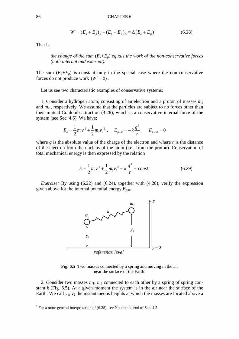
86 CHAPTER 6
y
0y =
1y2y
1m
2m
k
reference level
( ) ( ) ( )k p B k p A k pW E E E E E E′ = + − + ≡ ∆ + (6.28)
That is,
the change of the sum (Ek+Ep) equals the work of the non-conservative forces (both internal and external).1
The sum (Ek+Ep) is constant only in the special case where the non-conservative forces do not produce work ( 0)W′ = . Let us see two characteristic examples of conservative systems: 1. Consider a hydrogen atom, consisting of an electron and a proton of masses m1 and m2 , respectively. We assume that the particles are subject to no forces other than their mutual Coulomb attraction (4.28), which is a conservative internal force of the system (see Sec. 4.6). We have:
2
2 21 1 2 2 ,int ,ext
1 1, , 0
2 2k p p
qE m v m v E k E
r= + = − =
where q is the absolute value of the charge of the electron and where r is the distance of the electron from the nucleus of the atom (i.e., from the proton). Conservation of total mechanical energy is then expressed by the relation
2
2 21 1 2 2
1 1.
2 2
qE m v m v k const
r= + − = (6.29)
Exercise: By using (6.22) and (6.24), together with (4.28), verify the expression given above for the internal potential energy Ep,int .
Fig. 6.5 Two masses connected by a spring and moving in the air near the surface of the Earth.
2. Consider two masses m1, m2 connected to each other by a spring of spring con-stant k (Fig. 6.5). At a given moment the system is in the air near the surface of the Earth. We call y1, y2 the instantaneous heights at which the masses are located above a
1 For a more general interpretation of (6.28), see Note at the end of Sec. 4.5.
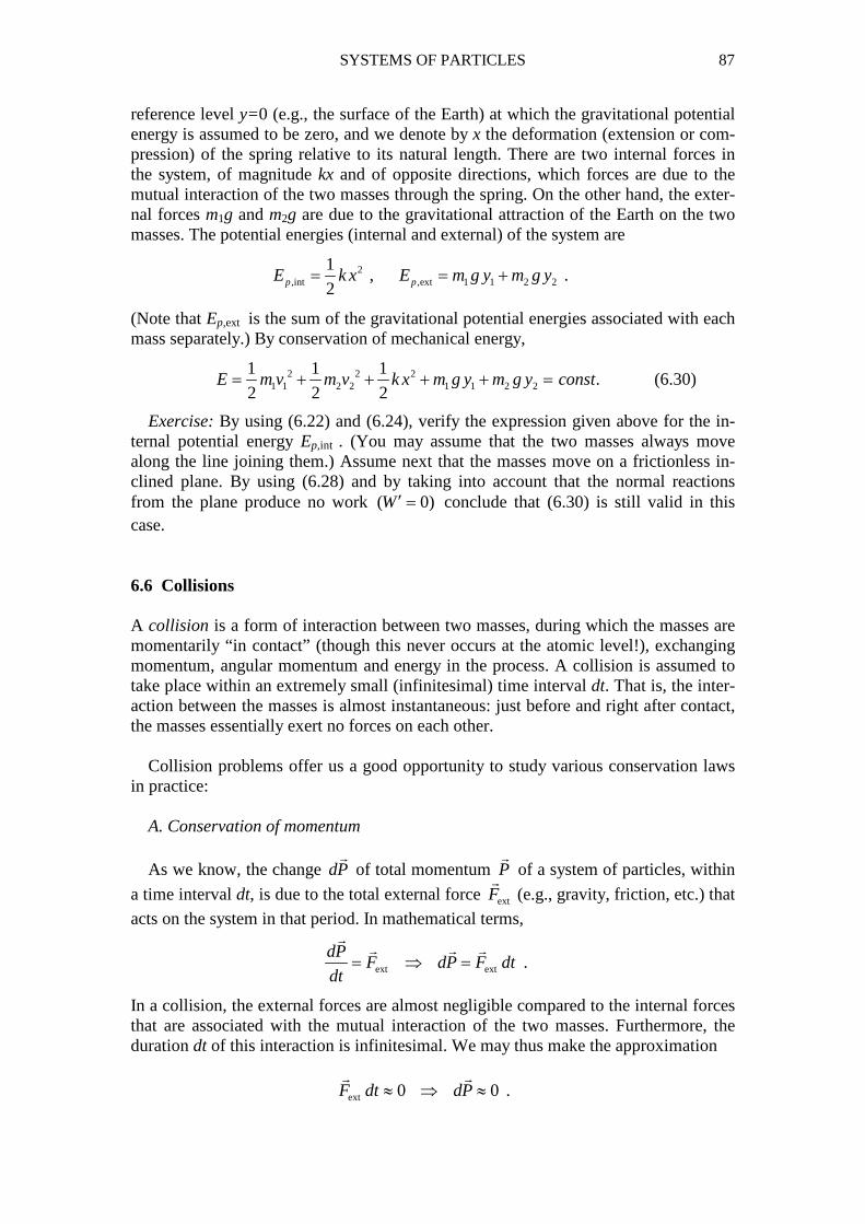
SYSTEMS OF PARTICLES 87
reference level y=0 (e.g., the surface of the Earth) at which the gravitational potential energy is assumed to be zero, and we denote by x the deformation (extension or com-pression) of the spring relative to its natural length. There are two internal forces in the system, of magnitude kx and of opposite directions, which forces are due to the mutual interaction of the two masses through the spring. On the other hand, the exter-nal forces m1g and m2g are due to the gravitational attraction of the Earth on the two masses. The potential energies (internal and external) of the system are
2,int ,ext 1 1 2 2
1,
2p pE k x E m g y m g y= = + .
(Note that Ep,ext is the sum of the gravitational potential energies associated with each mass separately.) By conservation of mechanical energy,
2 2 21 1 2 2 1 1 2 2
1 1 1.
2 2 2E m v m v k x m g y m g y const= + + + + = (6.30)
Exercise: By using (6.22) and (6.24), verify the expression given above for the in-ternal potential energy Ep,int . (You may assume that the two masses always move along the line joining them.) Assume next that the masses move on a frictionless in-clined plane. By using (6.28) and by taking into account that the normal reactions from the plane produce no work ( 0)W′ = conclude that (6.30) is still valid in this case. 6.6 Collisions A collision is a form of interaction between two masses, during which the masses are momentarily “in contact” (though this never occurs at the atomic level!), exchanging momentum, angular momentum and energy in the process. A collision is assumed to take place within an extremely small (infinitesimal) time interval dt. That is, the inter-action between the masses is almost instantaneous: just before and right after contact, the masses essentially exert no forces on each other. Collision problems offer us a good opportunity to study various conservation laws in practice: A. Conservation of momentum As we know, the change dP
�
of total momentum P�
of a system of particles, within
a time interval dt, is due to the total external force extF�
(e.g., gravity, friction, etc.) that
acts on the system in that period. In mathematical terms,
ext ext
dPF dP F dt
dt= ⇒ =
�
� � �
.
In a collision, the external forces are almost negligible compared to the internal forces that are associated with the mutual interaction of the two masses. Furthermore, the duration dt of this interaction is infinitesimal. We may thus make the approximation
ext 0 0F dt dP≈ ⇒ ≈� �
.
88 CHAPTER 6
We conclude that
the total momentum of the system is unchanged in a collision; that is, the mo-mentum just before the collision equals the momentum right after the collision.
B. Conservation of angular momentum The change dL
�
of total angular momentum of a system, relative to some point O,
and the total external torque extT�
on the system, relative to O, are related by
ext ext
dLT dL T dt
dt= ⇒ =
�
� � �
.
As before,
ext 0 0T dt dL≈ ⇒ ≈� �
.
That is,
in a collision, the total angular momentum of the system, relative to any point, is unchanged (i.e., the values of the angular momentum just before and right after the collision are the same).
C. Kinetic energy In contrast to momentum and angular momentum, kinetic energy is not necessarily conserved in a collision. This is explained as follows: We recall that the change of total kinetic energy of a system, within a time period (here, the time dt of duration of the collision), equals the work of the external and the internal forces acting on the sys-tem in that period. Even if we assume that, for reasons explained previously, the work of the external forces within an infinitesimal time interval is negligible, we cannot ig-nore the work of the internal forces, which is particularly significant if the collision produces a deformation of the colliding bodies. In such a case, part of the initial ki-netic energy of the system is lost due to the (negative) work done by the internal forces that are responsible for this deformation. Collisions are classified on the basis of conservation or non-conservation of kinetic energy, as follows: a. Elastic collision: The total kinetic energy of the system of colliding bodies is un-changed by the collision. That is, the kinetic energies just before and right after the collision are equal. This is the case for collisions that do not cause deformation of the colliding bodies. Example: the collision of two hard billiard balls. b. Inelastic collision: Part of the kinetic energy of the system is lost due to deformation caused by the collision; this energy is thus not conserved in the process. Example: the collision of two rubber balls. c. Completely inelastic (or plastic) collision: This is an extreme form of inelastic collision in which the colliding bodies stick together and move as one body, with common final velocity. Part of the initial kinetic energy of the system is lost due to
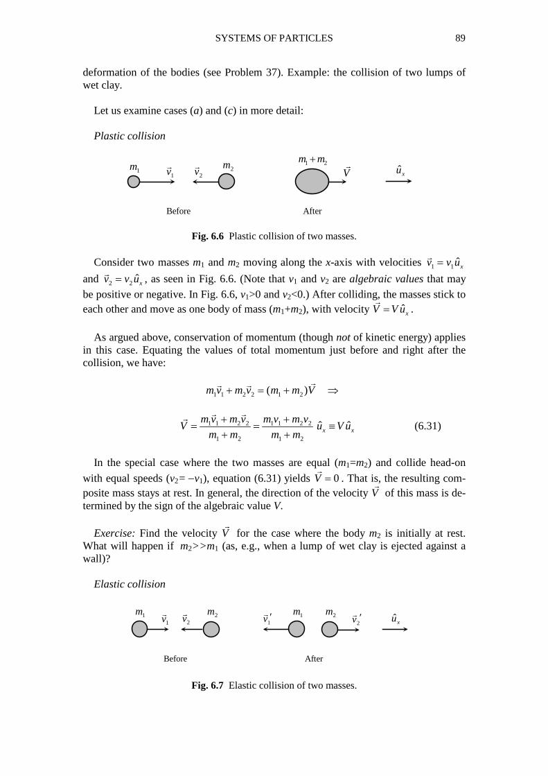
SYSTEMS OF PARTICLES 89
deformation of the bodies (see Problem 37). Example: the collision of two lumps of wet clay. Let us examine cases (a) and (c) in more detail: Plastic collision
Fig. 6.6 Plastic collision of two masses. Consider two masses m1 and m2 moving along the x-axis with velocities 1 1 ˆxv v u=
�
and 2 2 ˆxv v u=�
, as seen in Fig. 6.6. (Note that v1 and v2 are algebraic values that may
be positive or negative. In Fig. 6.6, v1>0 and v2<0.) After colliding, the masses stick to each other and move as one body of mass (m1+m2), with velocity ˆxV V u=
�
.
As argued above, conservation of momentum (though not of kinetic energy) applies in this case. Equating the values of total momentum just before and right after the collision, we have: 1 1 2 2 1 2( )m v m v m m V+ = + ⇒
�� �
1 1 2 2 1 1 2 2
1 2 1 2
ˆ ˆx x
m v m v m v m vV u V u
m m m m
+ += = ≡
+ +
� ��
(6.31)
In the special case where the two masses are equal (m1=m2) and collide head-on
with equal speeds (v2= −v1), equation (6.31) yields 0V =�
. That is, the resulting com-posite mass stays at rest. In general, the direction of the velocity V
�
of this mass is de-termined by the sign of the algebraic value V. Exercise: Find the velocity V
�
for the case where the body m2 is initially at rest. What will happen if m2>>m1 (as, e.g., when a lump of wet clay is ejected against a wall)? Elastic collision
Fig. 6.7 Elastic collision of two masses.
1m 2m 1 2m m+
1v�
2v�
V� ˆxu
AfterBefore
1m 2m 2m1m1v�
1v ′�
2v ′�2v�
ˆxu
Before After
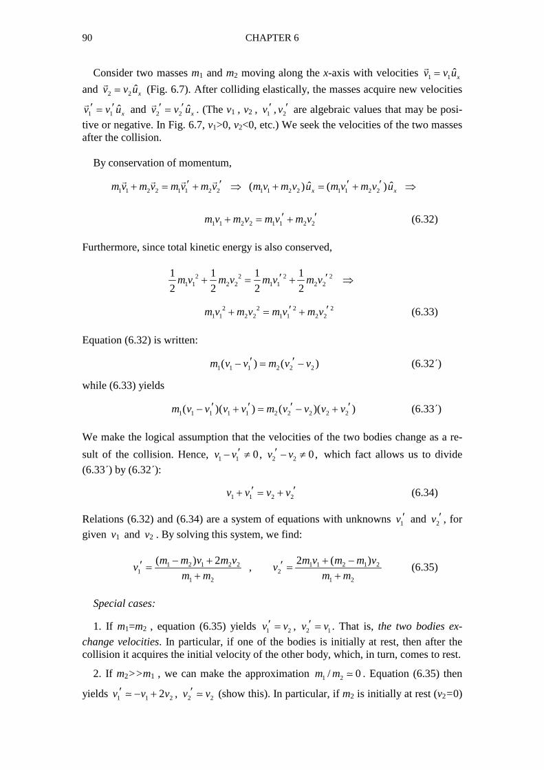
90 CHAPTER 6
Consider two masses m1 and m2 moving along the x-axis with velocities 1 1 ˆxv v u=�
and 2 2 ˆxv v u=�
(Fig. 6.7). After colliding elastically, the masses acquire new velocities
1 1 ˆxv v u′ ′=�
and 2 2 ˆxv v u′ ′=�
. (The v1 , v2 , 1v ′ , 2v ′ are algebraic values that may be posi-
tive or negative. In Fig. 6.7, v1>0, v2<0, etc.) We seek the velocities of the two masses after the collision. By conservation of momentum,
1 1 2 2 1 1 2 2 1 1 2 2 1 1 2 2ˆ ˆ( ) ( )x xm v m v m v m v m v m v u m v m v u′ ′ ′ ′+ = + ⇒ + = + ⇒� � � �
1 1 2 2 1 1 2 2m v m v m v m v′ ′+ = + (6.32)
Furthermore, since total kinetic energy is also conserved,
2 2 2 21 1 2 2 1 1 2 2
1 1 1 1
2 2 2 2m v m v m v m v′ ′+ = + ⇒
2 2 2 21 1 2 2 1 1 2 2m v m v m v m v′ ′+ = + (6.33)
Equation (6.32) is written:
1 1 1 2 2 2( ) ( )m v v m v v′ ′− = − (6.32)
while (6.33) yields
1 1 1 1 1 2 2 2 2 2( )( ) ( )( )m v v v v m v v v v′ ′ ′ ′− + = − + (6.33)
We make the logical assumption that the velocities of the two bodies change as a re-
sult of the collision. Hence, 1 1 2 20, 0,v v v v′ ′− ≠ − ≠ which fact allows us to divide
(6.33 ) by (6.32):
1 1 2 2v v v v′ ′+ = + (6.34)
Relations (6.32) and (6.34) are a system of equations with unknowns 1v ′ and 2v ′ , for
given v1 and v2 . By solving this system, we find:
1 2 1 2 2 1 1 2 1 21 2
1 2 1 2
( ) 2 2 ( ),
m m v m v m v m m vv v
m m m m
− + + −′ ′= =+ +
(6.35)
Special cases:
1. If m1=m2 , equation (6.35) yields 1 2 2 1,v v v v′ ′= = . That is, the two bodies ex-
change velocities. In particular, if one of the bodies is initially at rest, then after the collision it acquires the initial velocity of the other body, which, in turn, comes to rest.
2. If m2>>m1 , we can make the approximation 1 2/ 0m m ≃ . Equation (6.35) then
yields 1 1 2 2 22 ,v v v v v′ ′− +≃ ≃ (show this). In particular, if m2 is initially at rest (v2=0)

SYSTEMS OF PARTICLES 91
then 1 1 2, 0v v v′ ′−≃ ≃ . That is, after the collision the body m2 remains at rest, while
the direction of motion of m1 is reversed with no change in this body’s speed.
References
1. C.J. Papachristou, Foundations of Newtonian Dynamics: An Axiomatic Ap-proach for the Thinking Student, Nausivios Chora, Vol. 4 (2012) 1532
2. J.B. Marion, S.T. Thornton, Classical Dynamics of Particles and Systems, 4th Edition (Saunders College, 1995)
3. D.J. Griffiths, Introduction to Electrodynamics, 4th Edition (Pearson, 2013)
2 http://nausivios.snd.edu.gr/docs/partC2012.pdf ; new version: https://arxiv.org/abs/1205.2326
92
CHAPTER 7
RIGID-BODY MOTION 7.1 Rigid Body A system of particles constitutes a rigid body if the relative positions and distances of the particles remain fixed when external forces or torques act on the system. Hence, a rigid body maintains its shape during its motion.1 A rigid body may execute two kinds of motion:
1. Translational motion, when all particles move with the same velocity and de-scribe parallel trajectories, so that the body stays parallel to itself at all times.
2. Rotational motion, when the particles describe circular paths about an axis of ro-tation. This axis may or may not be fixed in space during the rotation of the body. The most general motion of a rigid body is a combination of translation and rota-tion (notice, for example, the motion of a ball or a car wheel). An example of such a composite motion is a translation of the center of mass C of the body, with a simulta-neous rotation of the body about an axis passing through C. As we will see, the center of mass plays an important role in the dynamics of a rigid body. 7.2 Center of Mass of a Rigid Body We have seen (Sec. 6.2) that the center of mass C of a system of particles moves in space as if it were a particle of mass equal to the total mass M of the system, subject to the total external force acting on the system. The same is true for a rigid body if this body is viewed as a structure composed of a number of particles of masses mi . Let us assume that the only external forces acting on the system (or the rigid body) are those due to gravity. The total external force is then equal to the total weight of the system:
( )i i ii i i
w w m g m g
= = = ⇒
∑ ∑ ∑� � � �
w M g=� �
where ii
M m=∑ (7.1)
The acceleration of gravity, g
�
, is constant in a limited region of space where the gravitational field may be considered uniform. Note that w
�
is a sum of forces acting on separate particles mi located at various points of space. The question now is whether there exists some specific point of appli-cation of the total weight w
�
of the system and, in particular, of a rigid body. A rea-sonable assumption is that this point could be the center of mass C of the body, given that, as mentioned above, the point C behaves as if it concentrates the entire mass Μ 1 More generally, a rigid body may consist of mobile parts. We will examine this case in Sec. 7.7.
RIGID-BODY MOTION 93
of the body and the total external force acting on it. And, in our case, w�
is indeed the total external force, due to gravity alone. There is a subtle point here, however. In contrast to a point particle (such as the hy-pothetical “particle” of mass M moving with the center of mass C ) that simply changes its location in space, a rigid body may execute a more complex motion; spe-cifically, a combination of translation and rotation. The translational motion of the body under the action of gravity is indeed represented by the motion of the center of mass C, if this point is regarded as a “particle” of mass Μ on which the total force w
�
is applied. For the rotational motion of the body, however, it is the torques of the ex-ternal forces, rather than the forces themselves, that are responsible. Where should we place the total force w
�
in order that the rotational motion it produces on the body be the same as that caused by the simultaneous action of the elementary gravitational forces i iw m g=
� �
? Equivalently, where should we place w�
in order that its torque with
respect to any point O be equal to the total torque of the iw�
with respect to O ?
You may have guessed the answer already: at the center of mass C (this will be shown analytically in Appendix A). In conclusion:
By placing the total weight w�
of the body at the center of mass C, we manage to describe both the translational and the rotational motion of the body under the action of gravity.
It is for this reason that C is frequently called the center of gravity of the body. Note that this point does not necessarily belong to the body (consider, for example, the cases of a ring or a spherical shell). In most cases a rigid body is an object exhibiting continuous mass distribution. Such an object can be considered as a system consisting of an enormous (practically infinite) number of particles of infinitesimal masses dmi , placed in such a way that the distance between any two neighboring particles is zero. The total mass of the body is
ii
M dm dm= =∑ ∫ (7.2)
where the sum has been replaced by an integral due to the fact that the dmi are infini-tesimal and the distribution of mass is continuous. A point in a rigid body can be specified by its position vector r
�
, or its coordinates (x, y, z), relative to the origin Ο of some frame of reference. Let dV be an infinitesimal volume centered at ( , , )r x y z≡
�
, and let dm be the infinitesimal mass contained in this volume element. The density ρ of the body at point r
�
is defined as
( ) ( , , )dm
r x y zdV
ρ ρ= =�
(7.3)
Then,
( )dm r dVρ=�

94 CHAPTER 7
and therefore, relation (7.2) for the total mass of the body is written:
( )M r dVρ= ∫�
(7.4)
where the integration takes place over the entire volume of the body. (The integral is in fact a triple one, since, in Cartesian coordinates, dV=dxdydz.) The center of mass C of the body is found by using (6.2):
1 1( )C i i
i
r dm r rdmM M
= = ⇒∑ ∫� � �
1
( )Cr r r dVM
ρ= ∫� � �
(7.5)
where the r
�
and Cr�
are measured relative to the origin Ο of our coordinate system.
(Remember, however, that the location of C with respect to the body is uniquely de-termined and is independent of the choice of the reference point Ο.) In a homogeneous body the density has a constant value ρ, independent of r
�
. Then,
M dV dV Vρ ρ ρ= = =∫ ∫ (7.6)
where V is the total volume of the body. Also, from (7.5) we have:
1
Cr r dV r dVM V
ρ= =∫ ∫� � �
(7.7)
Imagine now that, instead of a mass distribution in space, we have a linear distribu-tion of mass (e.g., a very thin rod) along the x-axis. We define the linear density of the distribution as
( )dm
xdx
ρ = (7.8)
The total mass of the distribution is
( )M dm x dxρ= =∫ ∫ (7.9)
The position of the center of mass of the distribution is given by
1 1
( )Cx x dm x x dxM M
ρ= =∫ ∫ (7.10)
If the density ρ is constant, independent of x, then
M dx dx lρ ρ ρ= = =∫ ∫ (7.11)

RIGID-BODY MOTION 95
ii x0x=
O C
Cxa a l+
where l is the total length of the distribution. Furthermore,
1
Cx x dx x dxM l
ρ= =∫ ∫ (7.12)
Fig. 7.1 The center of mass of a thin, homogeneous rod is at the center of the rod. As an example, consider a thin, homogeneous rod of length l, placed along the x-axis from x=a to x=a+l , as shown in Fig. 7.1. By equation (7.12),
2 21 1( )
2 2
a l
C a
lx x dx a l a a
l l
+ = = + − = + ∫ .
That is, the center of mass C of the rod is located at the center of the rod. Notice that the location of C on the rod is uniquely determined, independently of the choice of the origin Ο of the x-axis (although the value of the coordinate xC does, of course, depend on this choice). 7.3 Revolution of a Particle About an Axis As we have said, a rigid body can be viewed as a system of particles mi (or dmi , for a continuous mass distribution) the relative positions and distances of which are fixed. So, before we study the rotational motion of a rigid body, it would be helpful to exam-ine the revolution of a single particle m about an axis. The following analysis is fairly detailed and most of it may be skipped in a first reading; the student may thus concen-trate on the main physical conclusions.
Fig. 7.2 Circular motion of a particle about the z-axis. The right figure is a view of the left figure “from above”.
i
⋅
xy
zˆzu
+
R
m
L�
ˆTu
v�
i
r�
O
O′
•'x
'y
'Oθ
R�
+
v�
m
ˆRuˆTu
ˆRuˆTu
ˆzu
96 CHAPTER 7
•
O
O′
z
ˆzur�
R�
mˆRu
We choose the z-axis of our coordinate system to coincide with the axis of revolu-tion and we call R the (constant) perpendicular distance of m from this axis (see Fig. 7.2). The particle m thus describes a circle of radius R, centered at some point Ο΄ of the z-axis, where Ο΄ is the normal projection of m on the axis. The axes x΄ and y΄ in the right figure are parallel to the axes x and y, respectively, while the z-axis is normal to the page and the unit vector ˆzu is directed outward (toward the reader).
In accordance with the conventions established in Sections 2.6 and 2.7, the positive direction of traversing the circle is determined by the direction of the unit tangent vec-tor ˆTu and is independent of the actual direction of motion (in Fig. 7.2 the motion is in
the positive direction). By convention, the positive direction of revolution is related to the direction of zu by means of the right-hand rule; that is, by rotating our fingers in
the positive direction of revolution (i.e., in the direction of ˆTu ) our right thumb points
in the direction of zu . If R�
is the position vector of m relative to Ο΄, and if ˆRu is the
unit vector in the direction of R�
(so that ˆRR Ru=�
), the ordered triad ˆ ˆ ˆ( , , )R T zu u u
forms a right-handed rectangular system of unit vectors. This means that ˆ ˆ ˆ ˆ ˆ ˆ ˆ ˆ, ,R T z T z R z R Tu u u u u u u u u× = × = × = (7.13)
The velocity of the particle m is, according to (2.32) and (2.34), ˆTv vu=
�
where v R vω= = ±�
(7.14)
The angular velocity ω is positive for counterclockwise motion (as in Fig. 7.2) and negative for clockwise motion. The position vector of m with respect to Ο is (see Fig. 7.3)
ˆ ˆz Rr OO R zu Ru′= + = +����� ��
(7.15)
where the distance ΟΟ΄= z of Ο΄ from Ο is one of the three coordinates of m. In Fig. 7.3 the unit vector Tu (which determines the positive direction of revolution) is nor-
mal to the page and directed into it.
Fig. 7.3 The position vector of m, relative to O, is the sum of components in the z- and R-directions.
RIGID-BODY MOTION 97
O
z
L�
ˆzu
zL
The angular momentum of m with respect to the origin Ο of coordinates is ( )L m r v= ×
� � �
. By substituting for r�
and v�
from (7.15) and (7.14), respectively, and by using (7.13), we have: 2ˆ ˆ ˆ ˆ ˆ ˆ ˆ( ) ( ) ( ) ( )R z T R T z TL m Ru zu R u mR u u mzR u uω ω ω= + × = × + × ⇒
�
2 ˆ ˆz RL mR u mzR uω ω= −�
(7.16)
The z-component of angular momentum, i.e., the projection of L�
onto the z-axis (see Fig. 7.4) is the coefficient of zu in (7.16):
2
zL mRω= (7.17)
We notice that Lz has the same sign as ω. Thus, Lz is positive or negative, depending on whether the particle revolves in the positive or the negative direction, respectively. (In Fig. 7.4, Lz is positive.)
Fig. 7.4 Projection of the angular momentum vector onto the z-axis. It is of interest to compare the angular momentum L
�
relative to Ο with the angular momentum L′
�
relative to the center Ο΄ of the circular path. The position vector of m with respect to Ο΄ is R
�
; hence, by using (7.13) and (7.14), 2ˆ ˆ ˆ( ) ( ) ( )R T zL m R v m Ru R u mR uω ω′ = × = × =
� � �
(7.18)
The z-component of L′�
is
2z zL mR Lω′ = = (7.19)
where we have taken (7.17) into account. We notice that the component Lz of the an-gular momentum in the direction of the axis of revolution is independent of the point of the axis relative to which the angular momentum is taken. (Of course, the vector L
�
of the angular momentum does depend on the choice of that point!) This conclusion is of more general validity:

98 CHAPTER 7
The component of the total angular momentum of a rotating system in the di-rection of the axis of rotation assumes a unique value, independent of the choice of reference point on that axis (i.e., of the point of the axis relative to which the angular momentum is taken).
The quantity
2I mR= (7.20) is called the moment of inertia of m with respect to the axis of revolution. Thus, (7.17) takes on the form zL Iω= (7.21)
Relation (7.21) connects the z-component Lz of the angular momentum with the angu-lar velocity ω, in the same way that the relation p=mv connects the linear momentum with the linear velocity. Note the correspondence between m and I in these two rela-tions: the moment of inertia I is for rotational motion what the mass m is for linear motion. Let F
�
be the total force on m at some point of the particle’s circular trajectory. The torque of F
�
with respect to Ο (equal to the vector sum of the torques of all forces act-ing on m) is T r F= ×
� ��
. If L�
is the angular momentum of m relative to Ο, and if our reference frame, with origin Ο, is assumed to be inertial, then, by (3.38),
dL
Tdt
= ⇒
�
�
ˆ ˆ ˆ ˆ ˆ ˆ ˆ ˆ ˆ( ) .yx zx x y y z z x x y y z z x y z
dLd dL dLT u T u T u L u L u L u u u u
dt dt dt dt+ + = + + = + +
By equating the coefficients of ˆzu and by using (7.21), we have:
( )zz
dL d dT I I
dt dt dt
ωω= = =
(since I is time-independent). Calling
d
dt
ωα =
the angular acceleration of m, we finally have: zT Iα= (7.22)
If T R F′ = ×
� � �
is the torque of F�
with respect to Ο΄, then
zz
dL dLT T
dt dt
′ ′′′ = ⇒ =
�
�
.

RIGID-BODY MOTION 99
But, by (7.19) and (7.21),
z zL L Iω′ = = .
Thus, again,
z zT I Tα′ = = (7.23)
We conclude that
the component of the total torque in the direction of the axis of revolution as-sumes a unique value independent of the choice of reference point on that axis.
Note the formal analogy between (7.22) and Newton’s law, F=ma . Relation (7.22) allows us to determine the angular acceleration of m, given the z-component of the total torque (equivalently, the torque of the total force) acting on the particle. All we need now is a practical way to evaluate Tz . First off, the particle always moves in the x΄y΄-plane, which is parallel to the xy-plane. This means that the total force F
�
on m is a vector on the x΄y΄-plane. Such a vector can be decomposed into two orthogonal components in the directions of the unit vectors Ru and ˆTu :
ˆ ˆR R T TF F u F u= +�
(7.24)
In the above relation, FT is the component of F
�
in the tangential direction relative to the circular path of m, while FR is the component of F
�
in the radial direction. By us-ing (7.15) and (7.24) we find the torque of F
�
with respect to Ο :
ˆ ˆ ˆ ˆ( ) ( )
ˆ ˆ ˆ ˆ ˆ ˆ( ) ( ) ( )R z R R T T
T R T R z R T z T
T r F Ru zu F u F u
RF u u zF u u zF u u
= × = + × +
= × + × + × ⇒
� ��
ˆ ˆ ˆT z R T T RT RF u zF u zF u= + −�
(7.25)
The z-component of the torque is the coefficient of ˆzu in (7.25):
z TT RF= (7.26)
Note that Tz is independent of the location of the reference point Ο on the axis of revolution (since Tz is independent of z), in agreement with a remark made earlier.
Assume now that F�
is the resultant of a set of forces 1 2, , ,F F� �
⋯ acting on m :
1 2 ii
F F F F= + + =∑� � � �
⋯ .
If FiR and FiT are the components (radial and tangential, respectively) of iF�
, the
components FR and FT of the total force F�
are, in the spirit of equation (1.10),
,R i R T i Ti i
F F F F= =∑ ∑ .
100 CHAPTER 7
By (7.26), the z-component of the total torque on m is
1 2 1 2( )z i T T T T Ti
T R F R F F RF RF= = + + = + +∑ ⋯ ⋯
or
1 2z z z i zi
T T T T= + + =∑⋯ (7.27)
where
i z i TT RF= (7.28)
is the z-component of the torque of iF
�
. Note that (7.27) represents a sum of quantities
that may be positive or negative. Specifically, Tiz is positive (negative) when the com-ponent FiT of iF
�
in the direction of Tu is positive (negative). This, in turn, means that
iF�
tends to cause a revolution of m in the positive (negative) direction about the z-axis
when m is initially at rest. [As already mentioned, the positive direction of revolution (i.e., the direction of Tu ) is related to the direction of ˆzu by the right-hand rule.]
As an example, consider the case where the particle m is subject to three forces
1 2 3, , ,F F F� � �
as shown in Fig. 7.5. In this figure the z-axis is normal to the page and ˆzu
is directed outward (toward the reader). On the other hand, ˆTu is, by definition, in the
positive direction of revolution, which, in turn, is related to the direction of ˆzu by the
right-hand rule (in Fig. 7.5 the positive direction is counterclockwise).
•⋅O′
R
+
ˆTu
1θ
2θ
1F�
2F�
3F�
m
1TF
2TF
Fig. 7.5 Revolution of a particle subject to three forces, about the z-axis (only the projection O of this axis is shown).
Let F1 , F2 , F3 be the magnitudes of the three forces. The components of these forces in the direction of Tu (tangential components) are
1 1 1 2 2 2 3cos , cos , 0T T TF F F F Fθ θ= = − = .
The signs of 1TF and 2TF are consistent with the fact that 1F�
tends to produce a revo-
lution in the positive direction, while 2F�
tends to generate a revolution in the opposite
RIGID-BODY MOTION 101
direction. The vanishing of 3TF means that 3F�
(which passes through the center Ο΄)
cannot produce a revolution of m about the z-axis when m is initially at rest. The z-components of the torques are, according to (7.28), 1 1 1 1 2 2 2 2 3 3cos , cos , 0z T z T z TT RF RF T RF RF T RFθ θ= = = = − = = .
The z-component of the total torque is given by (7.27): 1 2 3 1 1 2 2( cos cos )z z z zT T T T R F Fθ θ= + + = − .
Finally, the angular acceleration of m is found from (7.22) and (7.20):
1 1 2 22
1( cos cos )z zT TF F
I mR mRα θ θ= = = − .
7.4 Angular Momentum of a Rigid Body Consider now a rigid body rotating about an axis, which we arbitrarily choose to be the z-axis (see Fig. 7.6). As always, the direction of ˆzu also defines the positive direc-
tion of rotation according to the right-hand rule. We assume that the body consists of a number of particles mi located at corresponding perpendicular distances Ri from the axis of rotation. In the course of the rotation every particle mi executes circular motion of radius Ri , centered at the normal projection of mi on the z-axis. All particles have the same angular velocity ω, equal to the angular velocity of rotation of the rigid body. (Can you explain this?)
i
i
i
zˆ zu
ω
+
iRim
iv�
ir�
iL�
O
Fig. 7.6 As the rigid body rotates about the z-axis, all particles composing the body revolve
about this axis with common angular velocity ω.
102 CHAPTER 7
In Fig. 7.6 the body rotates in the positive direction with angular velocity ω. The angular momentum of a particle mi , with respect to a point Ο of the axis of rotation, is
( )i i i iL m r v= � � �
.
The total angular momentum of the body, relative to Ο, is
( )i i i ii i
L L m r v= = ×∑ ∑� � � �
(7.29)
According to equation (1.10), the z-component of L�
equals the algebraic sum of the z-components of the iL
�
:
z izi
L L=∑ .
But, by (7.21) and (7.20),
2iz i i iL I m Rω ω= = .
Hence,
()z i ii i
L I Iω ω= =∑ ∑
where we have taken into account that ω is the same for all mi . We now define the moment of inertia of the body with respect to the axis of rota-tion:
2i i i
i i
I I m R= =∑ ∑ (7.30)
(Notice that this is the sum of the moments of inertia of all particles making up the rigid body.) Thus, finally, zL Iω= (7.31)
Relation (7.31) gives the z-component of the angular momentum of the body, with respect to Ο. It is clear from (7.30) and (7.31) that
the component of the angular momentum of a rigid body in the direction of the axis of rotation is independent of the choice of reference point on that axis, relative to which point the angular momentum is taken.
Indeed, the moment of inertia I in (7.31) is dependent only on the perpendicular dis-tances Ri of the mi from the axis of rotation, not on the distances r i of the particles from the reference point Ο. For this reason we (somewhat improperly) call Lz the “angular momentum of the rigid body with respect to the axis of rotation”. The vector L�
of the angular momentum, of course, is only defined relative to the point Ο and de-pends, in general, on the location of Ο on the axis of rotation.
RIGID-BODY MOTION 103
7.5 Rigid-Body Equations of Motion To the extent that a rigid body can be treated as a system of particles, its motion is governed by the physical laws stated in the previous chapter. This system can perform two kinds of motion, namely, translation and rotation. The former motion is deter-mined by the total external force acting on the body, while the latter motion is af-fected by the total external torque. The momentum of a rigid body represents the total momentum of the system of particles making up the body and is given by equation (6.9): CP M v=
� �
(7.32)
where Μ is the mass of the body and where Cv
�
is the velocity of the body’s center of
mass, C. If 1 2, ,F F� �
⋯ are the external forces acting on the body (such a force is the
weight w�
, having C as its point of application) the total external force on the body is
ext 1 2F F F F= + + =∑� � � �
⋯ (7.33)
From (6.7) and (7.32) we then have:
CC
dP dvF M M a
dt dt= = =∑� �
� �
(7.34)
where Ca
�
is the acceleration of the center of mass of the body. Relation (7.34) is the
equation for translational motion of the rigid body. Note that, for translational motion
it doesn’t matter where the component forces 1 2, ,F F� �
⋯ act on the body; all we need to consider is the resultant of these forces. On the other hand, the rotational motion of the body is determined by the total ex-ternal torque. This motion, therefore, is dependent upon the points of application of
the external forces. Let 1 2, ,T T� �
⋯ be the torques of 1 2, ,F F� �
⋯ relative to some point Ο
in space. The total external torque on the body, relative to Ο, is
ext 1 2T T T T= + + =∑� � � �
⋯ (7.35)
Also, let L
�
be the angular momentum of the body with respect to Ο, equal to the vec-tor sum of angular momenta of all particles making up the body. According to (6.17),
dL
Tdt
=∑�
�
(7.36)
In Sec. 6.3 we noted that this relation is valid in either of two cases: (a) when Ο is a fixed point in some inertial frame of reference, or (b) when Ο coincides with the cen-ter of mass C, even if that point is accelerating (hence cannot be fixed in any inertial frame).
104 CHAPTER 7
In the case of rotation about an axis, conventionally chosen to be the z-axis of our coordinate system, the torques and angular momenta will always be taken with respect to a point Ο of that axis. In accordance with what was said above, relation (7.36) can be used in either of two cases: (a) rotation about an axis passing through a point Ο that is either fixed or moving with constant velocity in some inertial frame, or (b) ro-tation about an axis passing through the center of mass C of the body, where C may move with constant velocity or may accelerate relative to an inertial observer, depend-ing on whether the total external force on the body is zero or different from zero, re-spectively [see (7.34)]. The vector equation (7.36) can be resolved into three algebraic equations by taking components. We have:
ˆ ˆ ˆx x y y z zT u T u T u T= + +∑ ∑ ∑ ∑�
[see (1.10)] where, e.g., ΣTz is the algebraic sum of the z-components of all torques acting on the body, with respect to the reference point Ο. Moreover,
ˆ ˆ ˆ ˆ ˆ ˆ( ) yx zx x y y z z x y z
dLdL d dL dLL u L u L u u u u
dt dt dt dt dt= + + = + +
�
.
Equating coefficients of zu , we get:
zz
dLT
dt=∑ (7.37)
But, by (7.31), zL Iω= , where ω is the angular velocity of rotation and where Ι is the
moment of inertia of the body with respect to the z-axis of rotation [see equation (7.30)]. By assuming that Ι is constant, we have:
( )zdL d dI I I
dt dt dt
ωω α= = =
where α=dω/dt is the angular acceleration of the rotating body. Thus, finally,
zT Iα=∑ (7.38)
Relation (7.38) is the equation for rotational motion of the body. Relations (7.34) and (7.38) together constitute the equations of motion of a rigid body. From (7.38) it follows that
the component of the total external torque in the direction of the axis of rota-tion is independent of the reference point on that axis, relative to which point the torques of the external forces are taken.
Indeed, the moment of inertia Ι in (7.38) depends only on the perpendicular distances of the masses making up the body from the z-axis. For this reason the algebraic sum ΣTz is often (albeit somewhat improperly) called the “total torque with respect to the axis of rotation”. Remember, however, that the vector representing the total external torque is always defined with respect to a point Ο of the axis.
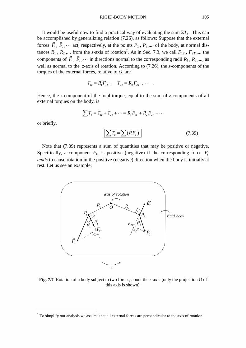
RIGID-BODY MOTION 105
•
+
⋅
⋅
O1P
2P
1R2R
1θ 2θ
1F�
2F�
1TF2TF
⋅
⋅
ˆTu′
ˆTu′′
axis of rotation
rigid body
It would be useful now to find a practical way of evaluating the sum ΣTz . This can be accomplished by generalizing relation (7.26), as follows: Suppose that the external
forces 1 2, ,F F� �
⋯ act, respectively, at the points P1 , P2 ,... of the body, at normal dis-
tances R1 , R2 ,... from the z-axis of rotation2. As in Sec. 7.3, we call F1T , F2T ,... the
components of 1 2, ,F F� �
⋯ in directions normal to the corresponding radii R1 , R2 ,..., as well as normal to the z-axis of rotation. According to (7.26), the z-components of the torques of the external forces, relative to Ο, are
1 1 1 2 2 2, ,z T z TT R F T R F= = ⋯ .
Hence, the z-component of the total torque, equal to the sum of z-components of all external torques on the body, is
1 2 1 1 2 2z z z T TT T T R F R F= + + = + +∑ ⋯ ⋯
or briefly,
( )z TT RF=∑ ∑ (7.39)
Note that (7.39) represents a sum of quantities that may be positive or negative. Specifically, a component FiT is positive (negative) if the corresponding force iF
�
tends to cause rotation in the positive (negative) direction when the body is initially at rest. Let us see an example:
Fig. 7.7 Rotation of a body subject to two forces, about the z-axis (only the projection O of
this axis is shown).
2 To simplify our analysis we assume that all external forces are perpendicular to the axis of rotation.
106 CHAPTER 7
In Fig. 7.7 the z-axis of rotation is normal to the page. The unit vector ˆzu is directed
outward (toward the reader), thus the positive direction of rotation is counterclock-wise. The external forces 1F
�
and 2F�
, acting at the points P1 and P2 of the body, are
normal to the z-axis (only the projection Ο of which axis is shown in the figure) and may belong to different planes parallel to each other and normal to the z-axis. The points P1 and P2 describe circular paths of radii R1 and R2 , respectively, where R1 and R2 are the perpendicular distances of these points from the axis of rotation. (The direc-tion of rotation of the body is not specified in the figure and is of no interest to us in
this particular problem.) The unit vectors ˆTu ′ and ˆTu ′′ , tangent to the circular paths of
P1 and P2 , respectively, always point toward the positive direction of rotation, regard-less of the actual direction of rotation of the body. The tangential components of 1F
�
and 2F�
are
1 1 1 2 2 2cos , cosT TF F F Fθ θ= = −
where F1 and F2 are the magnitudes of the two forces. The physical significance of the signs of F1T and F2T is that 1F
�
tends to rotate the body in the positive direction, while
2F�
tends to generate a rotation in the negative direction. The z-components of the ex-
ternal torques are
1 1 1 1 1 1 2 2 2 2 2 2cos , cosz T z TT R F R F T R F R Fθ θ= = = = − .
Thus, the total torque with respect to the axis of rotation is
1 2 1 1 1 2 2 2cos cosz z zT T T R F R Fθ θ= + = −∑ .
Finally, the angular acceleration of the body is, according to (7.38),
1 1 1 2 2 2
1 1( cos cos )zT R F R F
I Iα θ θ= = −∑
where I is the moment of inertia of the body with respect to the axis of rotation. 7.6 Moment of Inertia and the Parallel-Axis Theorem In the case of a rigid body consisting of a discrete set of particles m1, m2,..., the mo-ment of inertia with respect to an axis is 2 2 2
1 1 2 2i ii
I m R m R m R= = + +∑ ⋯ (7.40)
where Ri is the perpendicular distance of mi from the axis. As an example, consider two spheres of masses m1 and m2 connected to each other by a thin, weightless rod of length L, as seen in Fig. 7.8 (the role of the rod is simply to keep the spheres at a con-stant distance L from each other; the rod is thus not counted as part of the rigid body).
RIGID-BODY MOTION 107
x
L
O1m 2m1R 2R
Fig. 7.8 Rotating system of two spheres connected by a thin, weightless rod of length L. The moment of inertia of this system, with respect to an axis passing through Ο, is
2 2 2 21 1 2 2 1 2( )I m R m R m x m L x= + = + −
where we have put x=R1 . In particular, if the axis of rotation passes through m1, then x=0 and I=m2L
2 . As can be proven (see below) the moment of inertia assumes a minimum value when the axis of rotation passes through the center of mass C of the system. It is thus easier to rotate the system about such an axis, since a given external torque will then produce a maximum angular acceleration, according to (7.38). For rigid bodies consisting of a continuous distribution of matter, the sum in (7.40) must be replaced by an integral:
2I R dm= ∫ (7.41)
where R is the perpendicular distance of the elementary mass dm from the axis of rotation. This mass is written dm=ρdV , where ρ is the density of the body at the point where dm is located, and where dV is the volume occupied by dm. For a homogeneous body the density ρ is constant, equal to ρ=M/V , where M is the mass and V is the total volume of the body. Relation (7.41) is then written:
2 2 2MI R dV R dV R dV
Vρ ρ= = =∫ ∫ ∫ (7.42)
To evaluate the above integrals one must know the specific geometrical characteristics of the rigid body. A table of moments of inertia for the most common geometries is given in Appendix C. The parallel-axis theorem (or Steiner’s theorem) allows us to calculate the moment of inertia of a rigid body with respect to an axis, given the moment of inertia with re-spect to a parallel axis passing through the center of mass of the body. We state this theorem without proof (see [1,2]). Consider a rigid body of mass Μ. Let I be the mo-ment of inertia of the body with respect to an axis, and let IC be the moment of inertia with respect to a parallel axis passing through the center of mass C of the body. If the perpendicular distance between the two axes is equal to a, then
2CI I M a= + (7.43)
According to (7.43), given an infinite set of axes parallel to one another, the mo-ment of inertia of a rigid body becomes a minimum when taken with respect to the axis passing through the center of mass of the body. It is for this reason that, as men-
108 CHAPTER 7
i i
A C
2
l
2
l
2
l−
x0x =
dx
dm
x
S
tioned earlier, it is easiest to rotate a body about an axis passing through its center of mass C. (Of course, an infinite number of axes pass through C, each axis defining a separate infinity of parallel axes.) As an application of (7.42), we will calculate the moment of inertia of a thin rod of length l and mass M (see Fig. 7.9) with respect to an axis perpendicular to the rod and passing through its center C (which point coincides with the center of mass of the rod, as shown in an example at the end of Sec. 7.2). We call S the cross-sectional area of the rod and we assume that the rod lies on the x-axis.
Fig. 7.9 A thin rod of length l, lying along the x-axis.
We assume that the center C of the rod is located at the point x=0 of the axis, so that the rod extends from x= −l/2 to x= l/2 (this choice has no effect on the value of the moment of inertia, since this value depends only on the position of the axis of ro-tation relative to the body). We consider an elementary section of the rod, from x to x+dx. The volume of this section is dV=Sdx, while the total volume of the rod is V=S l. The distance R of the point x from the center of mass C (thus also the perpen-dicular distance of x from the axis that passes through C ) is R=|x| . Relation (7.42) is written (with I=I C for an axis passing through C ):
/ 23/ 2 2
/ 2/ 2
3
ll
C ll
M M xI S x dx
V l−−
= = ⇒
∫
21
12CI M l= (7.44)
To find the moment of inertia of the rod with respect to a parallel axis passing through an end of it – say, the end Α of the rod – we use (7.43) with a=l /2 :
2 2 21 1
12 4A CI I M a M l M l= + = + ⇒
21
3AI M l= (7.45)
Of course, the same result can be found directly from (7.42) (show this).

RIGID-BODY MOTION 109
7.7 Conservation of Angular Momentum Up to this point we have treated the moment of inertia Ι as a constant quantity, un-changed with time. This is true as long as the shape of the rigid body doesn’t change in the course of the body’s motion. We will now relax this requirement and consider rigid bodies whose shape may change while they move. This is, e.g., the case with the human body and, in general, with rigid bodies consisting of mobile parts. In such cases the moment of inertia with respect to an axis is a variable quantity and its change with time may significantly affect the rotational motion of the body even in the absence of external torques. The treatment of such complex problems, as well as of many others of a different nature (e.g., problems combining collision with rotational motion; see Problems 44 and 45) is simplified by using conservation of angular momentum, provided, of course, that the conditions for validity of this principle are fulfilled. As we know (Sec. 7.5) the angular momentum of a rigid body and the total external torque on the body are related by
dL
Tdt
=∑�
�
(7.46)
As stressed in Sec. 7.5, the above relation is valid for rotation about an axis passing through the common reference point Ο of L
�
and T�
, where Ο may be a fixed point in some inertial reference frame or may coincide with the center of mass C of the body
(even if C accelerates relative to an inertial observer). We notice that, if Σ 0T =�
, then
/ 0 .dL dt L const= ⇒ =� �
; that is,
when the total external torque on a rigid body, relative to a point Ο, is zero, the angular momentum of the body relative to Ο is constant in time.
This conclusion constitutes the principle of conservation of angular momentum for a rigid body. Note carefully that the vector relation (7.46) is always understood to be valid with respect to a point Ο. By taking the z-component of (7.46), however, we find an alge-braic relation that is valid with respect to the z-axis of rotation, regardless of the posi-tion of the reference point Ο on that axis (see Sec. 7.5):
zz
dLT
dt=∑ (7.47)
In particular, when ΣTz=0 , the component Lz of angular momentum is constant:
When the total external torque on the body relative to the axis of rotation is zero, the angular momentum of the body relative to this axis is constant in time.
110 CHAPTER 7
The above statement expresses the principle of conservation of angular momentum with respect to the axis of rotation. We remark that the choice of the z-axis of our coordinate system as coincident with the axis of rotation is totally arbitrary! We could have named our axes differently so that, e.g., the axis of rotation would be the x-axis or the y-axis. Relation (7.47) would then have to be rewritten with x or y in place of z. Now, according to (7.31), Lz=Iω, where ω is the angular velocity of rotation and where I is the moment of inertia of the rigid body relative to the z-axis of rotation. Thus, the constancy of angular momentum with respect to this axis is expressed as 1 1 2 2constantI I Iω ω ω= ⇔ = (7.48)
where the indices 1 and 2 refer to two moments t1 and t2 . If Ι is constant (Ι1=Ι2), which occurs when the geometry of the body is unchanged, the angular velocity ω is constant in time (ω1=ω2). This conclusion also follows from (7.38), according to which the angular acceleration α is zero (hence, the angular velocity ω is constant) when the total torque with respect to the axis of rotation vanishes. We talked earlier about a basic difference between the vector relation (7.46) and the algebraic relation (7.47). In (7.46) the L
�
and T�
are evaluated with respect to a point Ο of the axis of rotation and, generally, depend on the choice of this point, whereas in (7.47) the Lz and Tz are taken with respect to the axis itself and do not depend on the location of the reference point Ο on this axis. For each body, however, there is always a special set of axes of rotation, each of which passes through the center of mass C of the body and possesses the following property: the vector L
�
of the angular momen-
tum of the body [thus, by (7.46), the total external torque T�
also] does not depend on the choice of reference point Ο on that axis but assumes a unique value for all points of the axis. Furthermore, the angular momentum L
�
is directed parallel to the axis. An axis of rotation having these properties is called a principal axis. In particu-lar, every axis of symmetry passing through the center of mass C of the body is a principal axis for this body. Thus, in the case of a sphere, every axis passing through its center is a principal axis. For a cylinder, the central axis as well as every axis nor-mal to it and going through the center of mass are principal axes. For a cube, the three axes normal to the faces and passing through the center of the cube are principal axes. (More on principal axes will be said in Appendix D. See also [2,3].) Assume now that the z-axis of rotation is a principal axis of the rigid body (as men-tioned above, such an axis always passes through the center of mass C of the body). The angular momentum L
�
of the body, with respect to any point of this axis, will be independent of the location of that point on the axis and equal to ˆzL I uω=
�
(7.49)
where ω is the angular velocity of rotation and where Ι is the moment of inertia with respect to the principal axis (remember that ω may be positive or negative, depending on the direction of rotation).

RIGID-BODY MOTION 111
We define the angular velocity vector ˆzuω ω=
�
(7.50)
Equation (7.49) is then written:
L I ω=� �
(7.51) Relation (7.51) gives the angular momentum of a rigid body with respect to any point of a principal axis. Note that the angular momentum is directed parallel to the princi-pal axis. It must be noted here that a relation of the form (7.51) may sometimes be valid for axes that are not principal. For example, (7.51) gives the angular momentum L
�
of a thin flat plate rotating about an axis perpendicular to the plate, or of a rod rotating about an axis normal to it. Careful, however: In each of these examples the angular momentum L
�
is taken with respect to the point Ο of the body through which the axis passes! For any other point, (7.51) is not valid, unless the axis of rotation is a princi-pal axis (such as is, e.g., the axis normal to a circular disk and passing through the center of the disk, or, the axis intersecting a rod perpendicularly at its center). Let us now assume that, for any of the above reasons, relation (7.51) is valid rela-tive to a point O of the rotation axis. The fundamental equation (7.46) is then written, relative to this point,
( )dL d
T Idt dt
ω= =∑�
� �
(7.52)
If the moment of inertia Ι is constant,
d
T I Idt
ωα= =∑
�� �
(7.53)
where α
�
is the angular acceleration vector. If it happens that the total external torque
on the body, relative to O, is zero ( 0TΣ =�
), then, by (7.52), the angular momentum
L�
with respect to that point is constant:
1 1 2 2constantL I I Iω ω ω= = ⇔ =� � � �
(7.54)
Moreover, if Ι is constant, the angular acceleration α
�
is zero and the angular velocity ω�
is constant, as follows from (7.53) and (7.54). Let us see some examples: 1. Consider a body of mass Μ moving in space under the sole action of gravity; that is, no forces act on the body other than its weight w M g=
� �
. Hence, as explained in Sec. 7.2, the total external force on the body can be considered acting at the center of mass C (even if that point does not belong to the body, as, e.g., in the cases of a ring

112 CHAPTER 7
or a spherical shell). Then, the total torque with respect to C is zero and, according to (7.46), the angular momentum L
�
of the body relative to C is constant:
If a body moves under the sole action of gravity, the angular momentum of the body relative to its center of mass is constant.
What does a diver do in order to increase his angular speed and make several som-ersaults in the air? He allows his body to contract as much as possible by pulling hands and feet close to the trunk of his body, thus decreasing his moment of inertia relative to the axis of rotation (which axis is horizontal and passes through the center of mass C of the athlete). According to (7.48) and (7.54), this results in an increase of the magnitude of the angular velocity of rotation, ω
�
, of the body. [We assume that (7.51) is approximately valid when L
�
is taken with respect to C.] 2. You may have observed the spinning motion of a figure skater on ice. The skater is subject to two forces, namely, her weight and the normal reaction from the ice (we assume that friction is negligible). None of these forces produces torque with respect to the center of mass C of the skater; hence, the angular momentum of the skater rela-tive to C is constant. Moreover, the vertical axis of rotation is a principal axis, relative to which the conservation of angular momentum is expressed in the form (7.54) [or, algebraically, in the form (7.48)]. To increase her angular speed, the skater pulls her hands close to the trunk of her body, which has the effect of decreasing her moment of inertia. She does exactly the opposite in order to decrease her angular speed. 3. Why is a bicycle harder to overturn when it is in motion? Consider, for simplic-ity, a single bicycle wheel and call L
�
the angular momentum of the wheel with re-spect to its (principal) axis of rotation at time t. If T
�
is the total external torque on the wheel at this instant, the change of angular momentum within an infinitesimal time interval dt is dL T dt=
� �
. Now, an overturn of the wheel is accompanied by a change of
direction of L�
, which change requires a torque T�
perpendicular to L�
(in the same way that a force perpendicular to the velocity of a body is needed to produce a change of the direction of motion of the body). Then, the infinitesimal change dL
�
of the an-gular momentum will be normal to L
�
, as shown in Fig. 7.10.3
θL�
LdL+��
dL� T
�
Fig. 7.10 A torque normal to the angular momentum is needed in order to change the direction of the latter.
We notice that
| | | |
tan| | | |
dL T dt
L Lθ = =
� �
� � (7.55)
3 The figure is not drawn to scale. In fact, if the torque is normal to the angular momentum, then for dt→0 the magnitudes of the latter at times t and t+dt tend to be equal (see Sec. 7.12, below).
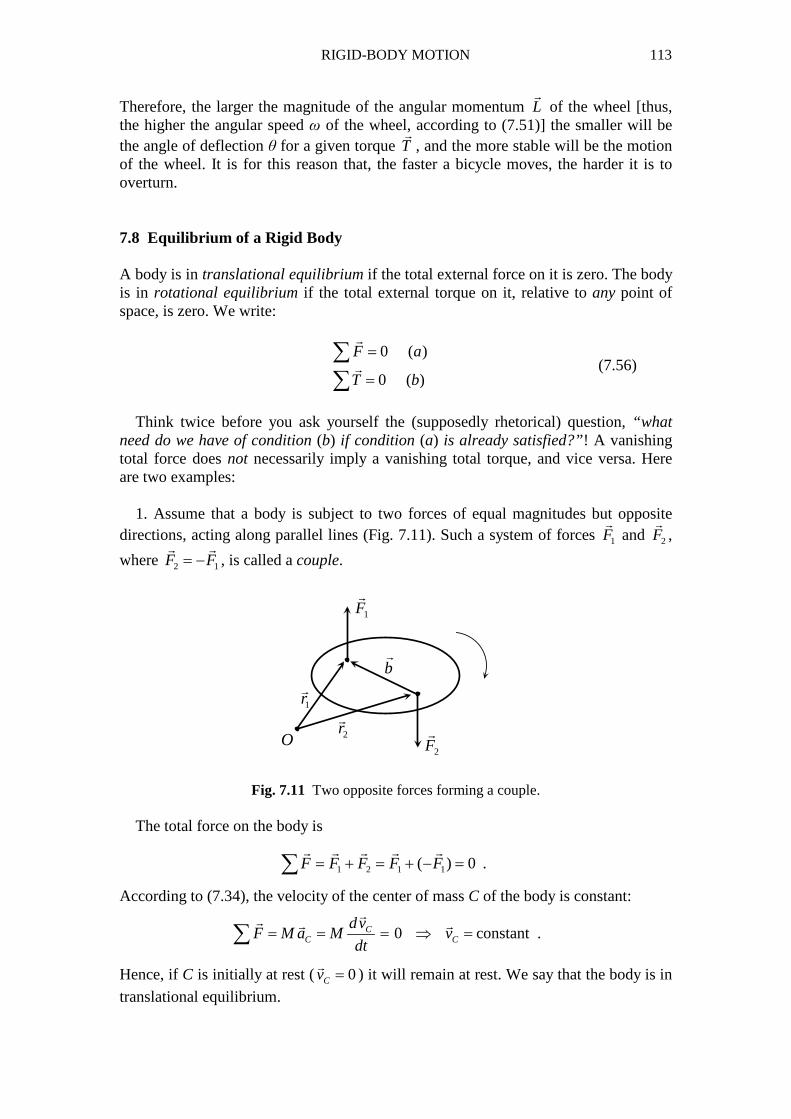
RIGID-BODY MOTION 113
Therefore, the larger the magnitude of the angular momentum L�
of the wheel [thus, the higher the angular speed ω of the wheel, according to (7.51)] the smaller will be the angle of deflection θ for a given torque T
�
, and the more stable will be the motion of the wheel. It is for this reason that, the faster a bicycle moves, the harder it is to overturn. 7.8 Equilibrium of a Rigid Body A body is in translational equilibrium if the total external force on it is zero. The body is in rotational equilibrium if the total external torque on it, relative to any point of space, is zero. We write:
0 ( )
0 ( )
F a
T b
=
=
∑∑
�
� (7.56)
Think twice before you ask yourself the (supposedly rhetorical) question, “what need do we have of condition (b) if condition (a) is already satisfied?”! A vanishing total force does not necessarily imply a vanishing total torque, and vice versa. Here are two examples: 1. Assume that a body is subject to two forces of equal magnitudes but opposite directions, acting along parallel lines (Fig. 7.11). Such a system of forces 1F
�
and 2F�
,
where 2 1F F= −� �
, is called a couple.
O
1r�
2r�
b�
1F�
2F�
Fig. 7.11 Two opposite forces forming a couple. The total force on the body is
1 2 1 1( ) 0F F F F F= + = + − =∑� � � � �
.
According to (7.34), the velocity of the center of mass C of the body is constant:
0 constantCC C
dvF M a M v
dt= = = ⇒ =∑
�� � �
.
Hence, if C is initially at rest ( 0Cv =�
) it will remain at rest. We say that the body is in
translational equilibrium.
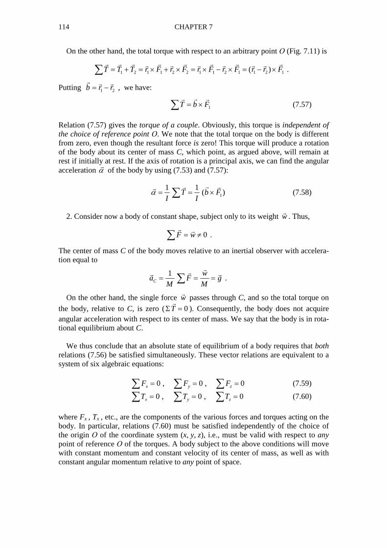
114 CHAPTER 7
On the other hand, the total torque with respect to an arbitrary point Ο (Fig. 7.11) is
1 2 1 1 2 2 1 1 2 1 1 2 1( )T T T r F r F r F r F r r F= + = × + × = × − × = − ×∑� � � � � � � �� � � � � �
.
Putting 1 2b r r= −�� �
, we have:
1T b F= ×∑�� �
(7.57)
Relation (7.57) gives the torque of a couple. Obviously, this torque is independent of the choice of reference point Ο. We note that the total torque on the body is different from zero, even though the resultant force is zero! This torque will produce a rotation of the body about its center of mass C, which point, as argued above, will remain at rest if initially at rest. If the axis of rotation is a principal axis, we can find the angular acceleration α
�
of the body by using (7.53) and (7.57):
1
1 1( )T b F
I Iα = = ×∑
�� ��
(7.58)
2. Consider now a body of constant shape, subject only to its weight w
�
. Thus,
0F w= ≠∑� �
.
The center of mass C of the body moves relative to an inertial observer with accelera-tion equal to
1
C
wa F g
M M= = =∑
��� �
.
On the other hand, the single force w�
passes through C, and so the total torque on
the body, relative to C, is zero ( 0TΣ =�
). Consequently, the body does not acquire angular acceleration with respect to its center of mass. We say that the body is in rota-tional equilibrium about C. We thus conclude that an absolute state of equilibrium of a body requires that both relations (7.56) be satisfied simultaneously. These vector relations are equivalent to a system of six algebraic equations: 0 , 0 , 0x y zF F F= = =∑ ∑ ∑ (7.59)
0 , 0 , 0x y zT T T= = =∑ ∑ ∑ (7.60)
where Fx , Tx , etc., are the components of the various forces and torques acting on the body. In particular, relations (7.60) must be satisfied independently of the choice of the origin Ο of the coordinate system (x, y, z), i.e., must be valid with respect to any point of reference Ο of the torques. A body subject to the above conditions will move with constant momentum and constant velocity of its center of mass, as well as with constant angular momentum relative to any point of space.
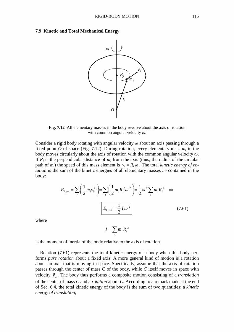
RIGID-BODY MOTION 115
7.9 Kinetic and Total Mechanical Energy
i
i
i
ω
iRim
iv�
ir�
O
Fig. 7.12 All elementary masses in the body revolve about the axis of rotation with common angular velocity ω.
Consider a rigid body rotating with angular velocity ω about an axis passing through a fixed point O of space (Fig. 7.12). During rotation, every elementary mass mi in the body moves circularly about the axis of rotation with the common angular velocity ω. If Ri is the perpendicular distance of mi from the axis (thus, the radius of the circular path of mi) the speed of this mass element is vi = Ri ω . The total kinetic energy of ro-tation is the sum of the kinetic energies of all elementary masses mi contained in the body:
2 2 2 2 2,rot
1 1 1
2 2 2k i i i i i ii i i
E m v m R m Rω ω = = = ⇒
∑ ∑ ∑
2,rot
1
2kE Iω= (7.61)
where
2i i
i
I m R=∑
is the moment of inertia of the body relative to the axis of rotation. Relation (7.61) represents the total kinetic energy of a body when this body per-forms pure rotation about a fixed axis. A more general kind of motion is a rotation about an axis that is moving in space. Specifically, assume that the axis of rotation passes through the center of mass C of the body, while C itself moves in space with velocity Cv
�
. The body thus performs a composite motion consisting of a translation
of the center of mass C and a rotation about C. According to a remark made at the end of Sec. 6.4, the total kinetic energy of the body is the sum of two quantities: a kinetic energy of translation,
116 CHAPTER 7
2,trans
1
2k CE M v= (7.62)
(where Μ is the mass of the body and vC is the speed of the center of mass C) and a kinetic energy of rotation about C,
2,rot
1
2k CE I ω= (7.63)
(where ω is the angular velocity of rotation about an axis passing through C, while IC is the moment of inertia of the body relative to that axis). The total kinetic energy of the body is, therefore,
2 2,trans ,rot
1 1
2 2k k k C CE E E M v I ω= + = + (7.64)
If the body is subject to external forces that are conservative, we can define an ex-ternal potential energy Ep as well as a total mechanical energy E, the latter assuming a constant value during the motion of the body:
2 21 1.
2 2k p C C pE E E M v I E constω= + = + + = (7.65)
For example, if the body moves under the sole action of gravity, its potential energy is p CE M g y= (7.66)
where yC is the vertical distance (the height) of the center of mass C with respect to an arbitrary horizontal plane of reference. Indeed, by relation (6.3),
1C i i
i
y m yM
= ∑
where yi is the height above the reference plane, of the location of the elementary mass mi in the body. The total gravitational potential energy of the body, equal to the sum of the potential energies of all elementary masses mi , is then
( )p i i i i Ci i
E m g y g m y M g y= = =∑ ∑ .
The total mechanical energy of the body is constant and equal to
2 21 1
2 2C C CE M v I M g yω= + + (7.67)
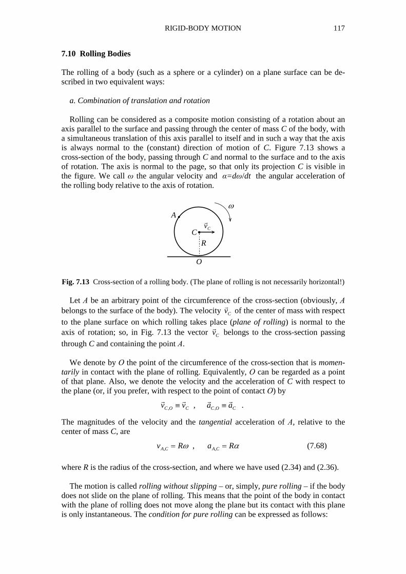
RIGID-BODY MOTION 117
7.10 Rolling Bodies The rolling of a body (such as a sphere or a cylinder) on a plane surface can be de-scribed in two equivalent ways: a. Combination of translation and rotation Rolling can be considered as a composite motion consisting of a rotation about an axis parallel to the surface and passing through the center of mass C of the body, with a simultaneous translation of this axis parallel to itself and in such a way that the axis is always normal to the (constant) direction of motion of C. Figure 7.13 shows a cross-section of the body, passing through C and normal to the surface and to the axis of rotation. The axis is normal to the page, so that only its projection C is visible in the figure. We call ω the angular velocity and α=dω/dt the angular acceleration of the rolling body relative to the axis of rotation.
i
O
C
R
Aω
Cv�
Fig. 7.13 Cross-section of a rolling body. (The plane of rolling is not necessarily horizontal!) Let Α be an arbitrary point of the circumference of the cross-section (obviously, Α belongs to the surface of the body). The velocity Cv
�
of the center of mass with respect
to the plane surface on which rolling takes place (plane of rolling) is normal to the axis of rotation; so, in Fig. 7.13 the vector Cv
�
belongs to the cross-section passing
through C and containing the point Α. We denote by Ο the point of the circumference of the cross-section that is momen-tarily in contact with the plane of rolling. Equivalently, Ο can be regarded as a point of that plane. Also, we denote the velocity and the acceleration of C with respect to the plane (or, if you prefer, with respect to the point of contact Ο) by
, ,,C O C C O Cv v a a≡ ≡� � � �
.
The magnitudes of the velocity and the tangential acceleration of Α, relative to the center of mass C, are
, ,,A C A Cv R a Rω α= = (7.68)
where R is the radius of the cross-section, and where we have used (2.34) and (2.36). The motion is called rolling without slipping – or, simply, pure rolling – if the body does not slide on the plane of rolling. This means that the point of the body in contact with the plane of rolling does not move along the plane but its contact with this plane is only instantaneous. The condition for pure rolling can be expressed as follows:
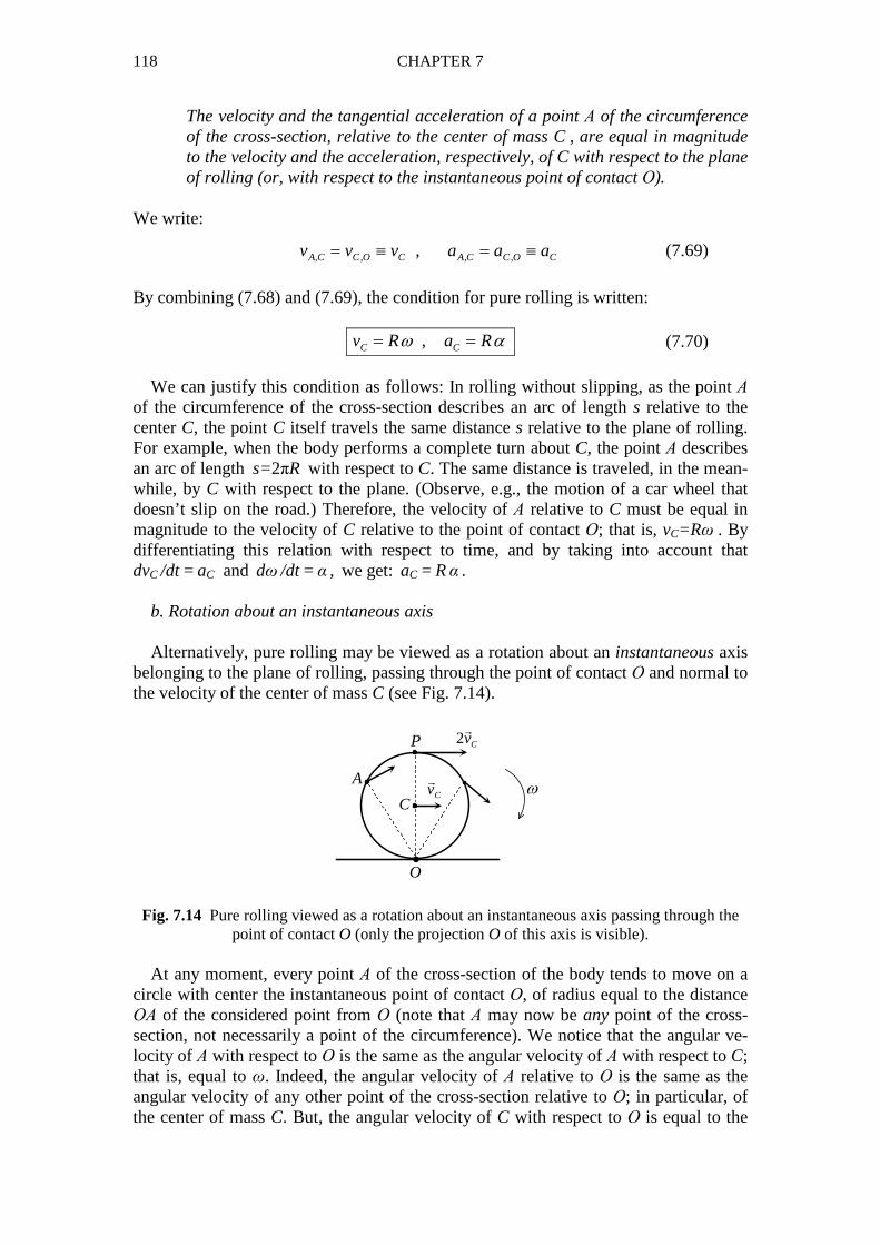
118 CHAPTER 7
The velocity and the tangential acceleration of a point Α of the circumference of the cross-section, relative to the center of mass C , are equal in magnitude to the velocity and the acceleration, respectively, of C with respect to the plane of rolling (or, with respect to the instantaneous point of contact Ο).
We write:
, , , ,,A C C O C A C C O Cv v v a a a= ≡ = ≡ (7.69)
By combining (7.68) and (7.69), the condition for pure rolling is written: ,C Cv R a Rω α= = (7.70)
We can justify this condition as follows: In rolling without slipping, as the point Α of the circumference of the cross-section describes an arc of length s relative to the center C, the point C itself travels the same distance s relative to the plane of rolling. For example, when the body performs a complete turn about C, the point Α describes an arc of length s=2πR with respect to C. The same distance is traveled, in the mean-while, by C with respect to the plane. (Observe, e.g., the motion of a car wheel that doesn’t slip on the road.) Therefore, the velocity of Α relative to C must be equal in magnitude to the velocity of C relative to the point of contact Ο; that is, vC=Rω . By differentiating this relation with respect to time, and by taking into account that dvC /dt = aC and dω /dt = α , we get: aC = R α . b. Rotation about an instantaneous axis Alternatively, pure rolling may be viewed as a rotation about an instantaneous axis belonging to the plane of rolling, passing through the point of contact Ο and normal to the velocity of the center of mass C (see Fig. 7.14).
iO
C
A
P
ωCv�
2 Cv�
Fig. 7.14 Pure rolling viewed as a rotation about an instantaneous axis passing through the
point of contact O (only the projection O of this axis is visible). At any moment, every point Α of the cross-section of the body tends to move on a circle with center the instantaneous point of contact Ο, of radius equal to the distance ΟΑ of the considered point from Ο (note that Α may now be any point of the cross-section, not necessarily a point of the circumference). We notice that the angular ve-locity of Α with respect to Ο is the same as the angular velocity of Α with respect to C; that is, equal to ω. Indeed, the angular velocity of Α relative to Ο is the same as the angular velocity of any other point of the cross-section relative to Ο; in particular, of the center of mass C. But, the angular velocity of C with respect to Ο is equal to the

RIGID-BODY MOTION 119
angular velocity of Ο with respect to C, which, in turn, is equal to ω. (Think of it as follows: Within an infinitesimal time interval dt, the angle described by C relative to the point Ο of the plane of rolling is the same as the angle described by the point Ο of the body relative to C.) Given that, momentarily, the motion of Α is circular about Ο, the speed of Α rela-tive to Ο (that is, relative to the plane of rolling) is
, ( )A Ov OAω= (7.71)
while the direction of motion of A is normal to the radius ΟΑ. If Α coincides with Ο, then (ΟΑ)=0 and
, 0O Ov = (7.72)
On the other hand, if Α coincides with C, then (ΟΑ)=(ΟC)=R and
,C O Cv v Rω≡ = (7.73)
By differentiating this with respect to time, we get:
,C O Ca a Rα≡ = (7.74)
We have thus recovered the condition (7.70) for pure rolling. Finally, if Α coincides with the top point Ρ of the cross-section (see Fig. 7.14) then (ΟΑ)=(ΟΡ)=2R and
, 2 2P O P Cv v R vω≡ = = (7.75)
Differentiating this with respect to time, we have:
, 2 2P O P Ca a R aα≡ = = (7.76)
7.11 The Role of Static Friction in Rolling In many cases (though not always) friction is necessary for rolling on a surface. Imag-ine, for example, a car at rest attempting to start moving on an icy road! The role of friction can be appreciated with the aid of the following example.
O
C
w�
f�
N�
Cv�
Fig. 7.15 Static friction is needed for pure rolling of a cylinder on an inclined plane.
120 CHAPTER 7
Consider a cylinder that is rolling without slipping on an inclined plane (Fig. 7.15). The angular velocity of the cylinder about the axis of rotation (which is a principal axis passing through the center of mass C ) increases as the cylinder rolls down the incline, which indicates the presence of an external torque with respect to C. What force can be responsible for that torque? Certainly, neither the weight w
�
nor the nor-mal reaction N
�
from the plane, since both these forces pass through C. The only re-
maining force is static friction f�
, the role of which is to prevent the cylinder from sliding on the incline (otherwise the motion would not be a pure rolling and, in that case, friction would be kinetic). We thus conclude that pure rolling would be impossi-ble on an inclined plane without the presence of static friction. (This conclusion is not valid, however, if the plane of rolling is horizontal; see Problem 47.) It should be noted that
in pure rolling the static friction does not produce work and thus has no effect on the conservation of mechanical energy.
[This is in contrast to rolling with slipping, where the friction is kinetic and does pro-duce (negative) work; see Sec. 4.7.] Indeed, in pure rolling the point of application Ο
of the static friction f�
does not move along the plane of rolling, since, according to (7.72), the instantaneous velocity of this point relative to the plane is zero. No work is
thus produced by f�
. 7.12 Gyroscopic Motion Generally speaking, the rotational motion of a body is characterized as gyroscopic if the axis of rotation passes through a fixed point of space but the direction of the axis changes with time. If the axis of rotation is a principal axis (e.g., an axis of symmetry, passing through the center of mass of the body) then, according to (7.49), the angular momentum L
�
of the body is directed parallel to that axis. Thus, in gyroscopic motion about a principal axis the direction of the angular momentum may change with time. In general, a change of the body’s angular momentum L
�
requires an external torque T
�
, where the vectors L�
and T�
are evaluated with respect to any point of the principal axis of rotation and are independent of the choice of that point. According to (7.46),
dL
T dL T dtdt
= ⇔ =
�
� � �
.
We notice that the infinitesimal change dL�
of the angular momentum is in the direc-tion of the external torque. If the torque T
�
is normal to the angular momentum L�
(see Fig. 7.10) the change dL�
is normal to L�
, so that 0L dL⋅ =� �
. But,
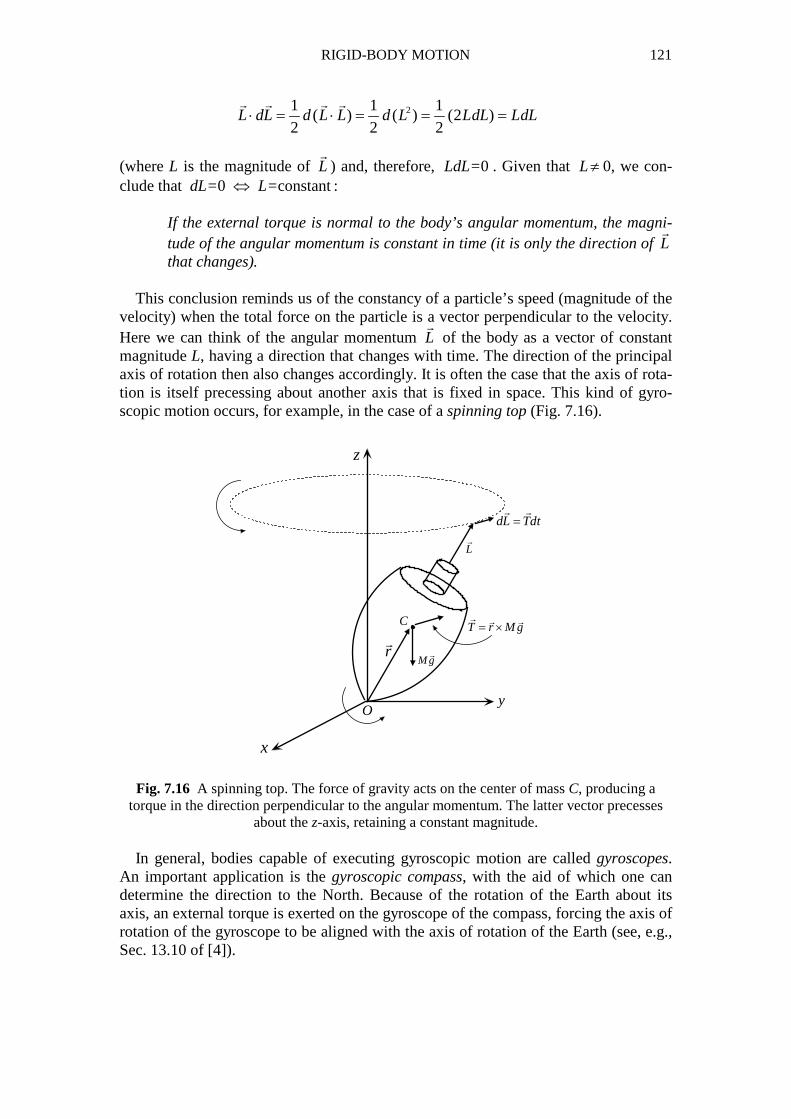
RIGID-BODY MOTION 121
21 1 1( ) ( ) (2 )
2 2 2L dL d L L d L LdL LdL⋅ = ⋅ = = =� � � �
(where L is the magnitude of L�
) and, therefore, LdL=0 . Given that L≠ 0, we con-clude that dL=0 ⇔ L=constant :
If the external torque is normal to the body’s angular momentum, the magni-tude of the angular momentum is constant in time (it is only the direction of L
�
that changes).
This conclusion reminds us of the constancy of a particle’s speed (magnitude of the velocity) when the total force on the particle is a vector perpendicular to the velocity. Here we can think of the angular momentum L
�
of the body as a vector of constant magnitude L, having a direction that changes with time. The direction of the principal axis of rotation then also changes accordingly. It is often the case that the axis of rota-tion is itself precessing about another axis that is fixed in space. This kind of gyro-scopic motion occurs, for example, in the case of a spinning top (Fig. 7.16).
Fig. 7.16 A spinning top. The force of gravity acts on the center of mass C, producing a
torque in the direction perpendicular to the angular momentum. The latter vector precesses about the z-axis, retaining a constant magnitude.
In general, bodies capable of executing gyroscopic motion are called gyroscopes. An important application is the gyroscopic compass, with the aid of which one can determine the direction to the North. Because of the rotation of the Earth about its axis, an external torque is exerted on the gyroscope of the compass, forcing the axis of rotation of the gyroscope to be aligned with the axis of rotation of the Earth (see, e.g., Sec. 13.10 of [4]).
x
y
z
O
C
r�
M g�
T r M g= � � �
L�
dL Tdt=� �
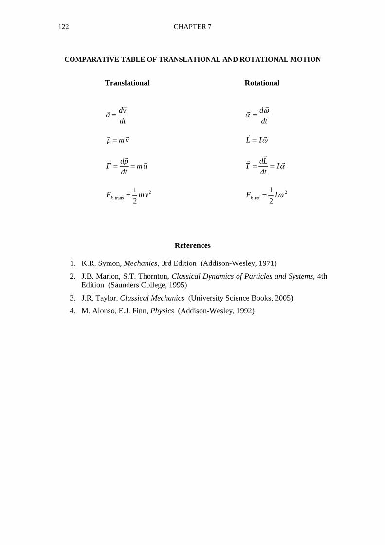
122 CHAPTER 7
COMPARATIVE TABLE OF TRANSLATIONAL AND ROTATIONAL M OTION
Translational Rotational
dv
adt
=�
�
d
dt
ωα =
�
�
p mv=
� �
L Iω=� �
dp
F madt
= =�
� �
dL
T Idt
α= =
�
� �
2,trans
1
2kE mv= 2,rot
1
2kE Iω=
References
1. K.R. Symon, Mechanics, 3rd Edition (Addison-Wesley, 1971)
2. J.B. Marion, S.T. Thornton, Classical Dynamics of Particles and Systems, 4th Edition (Saunders College, 1995)
3. J.R. Taylor, Classical Mechanics (University Science Books, 2005)
4. M. Alonso, E.J. Finn, Physics (Addison-Wesley, 1992)
123
CHAPTER 8
ELEMENTARY FLUID MECHANICS
8.1 Ideal Fluid The term “fluid” signifies a continuous medium that can flow. Depending on their physical properties (such as, e.g., compressibility) fluids are separated into liquids and gases. In this chapter we focus our attention to the study of liquids, and it is in this sense that the term “fluid” will be used henceforth. The mechanics of fluids can be separated into two parts; namely, Fluid Statics or Hydrostatics, which studies fluids at rest, and Fluid Dynamics or Hydrodynamics, which studies fluids in motion. Nothing in this world is ideal! This is not a pessimistic thought but simply an inter-pretation of the term “ideal” , which originates from the Greek word “ ιδέα” . It means something that exists only in our mind, an entity that is nonexistent in reality. Given that real fluids have physical characteristics (such as, e.g., viscosity) that make the theoretical study of these substances difficult, we invent an idealization of fluids with the generic name ideal fluid and with the following properties:
1. An ideal fluid is absolutely incompressible. This means that the density of an ideal fluid is the same at all points in the fluid. (As will be seen in Sec. 8.3, this assumption facilitates the derivation of the fundamental equation of Hy-drostatics.)
2. An ideal fluid is absolutely non-viscous (there is no internal friction within the fluid). This is particularly important in Hydrodynamics since it allows us to use conservation of mechanical energy for the study of fluid motion (this will be discussed in Sec. 8.12).
Many real fluids (e.g., water) have properties that are close to those of an ideal fluid. Note, however, that the characteristics of real fluids are not always undesirable. For example, if fluids were perfectly incompressible they would not allow the propa-gation of elastic waves (such as sound) in their interior. And, of course, you wouldn’t enjoy honey so much if it didn’t have that familiar thick texture! 8.2 Hydrostatic Pressure To begin our study of Hydrostatics we consider a liquid at rest in a vessel and we let ds be an elementary (i.e., infinitesimal) surface located at some point Σ in the fluid (see Fig. 8.1). The element ds may be part of the surface of an immersed object or may belong to a fictitious surface within the fluid (that is, a surface consisting of points belonging to the fluid itself). Such an elementary surface may be treated, at least approximately, as a plane surface. We call dF
�
the elementary force exerted by the fluid on ds.
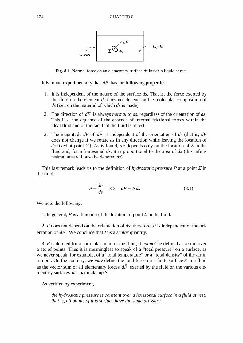
124 CHAPTER 8
Σ ds
dF�
vessel
liquid
Fig. 8.1 Normal force on an elementary surface ds inside a liquid at rest.
It is found experimentally that dF
�
has the following properties:
1. It is independent of the nature of the surface ds. That is, the force exerted by the fluid on the element ds does not depend on the molecular composition of ds (i.e., on the material of which ds is made).
2. The direction of dF�
is always normal to ds, regardless of the orientation of ds. This is a consequence of the absence of internal frictional forces within the ideal fluid and of the fact that the fluid is at rest.
3. The magnitude dF of dF�
is independent of the orientation of ds (that is, dF does not change if we rotate ds in any direction while leaving the location of ds fixed at point Σ ). As is found, dF depends only on the location of Σ in the fluid and, for infinitesimal ds, it is proportional to the area of ds (this infini-tesimal area will also be denoted ds).
This last remark leads us to the definition of hydrostatic pressure Ρ at a point Σ in the fluid:
dF
P dF Pdsds
= ⇔ = (8.1)
We note the following: 1. In general, Ρ is a function of the location of point Σ in the fluid. 2. Ρ does not depend on the orientation of ds; therefore, P is independent of the ori-entation of dF
�
. We conclude that Ρ is a scalar quantity. 3. Ρ is defined for a particular point in the fluid; it cannot be defined as a sum over a set of points. Thus it is meaningless to speak of a “total pressure” on a surface, as we never speak, for example, of a “total temperature” or a “total density” of the air in a room. On the contrary, we may define the total force on a finite surface S in a fluid as the vector sum of all elementary forces dF
�
exerted by the fluid on the various ele-mentary surfaces ds that make up S. As verified by experiment,
the hydrostatic pressure is constant over a horizontal surface in a fluid at rest; that is, all points of this surface have the same pressure.
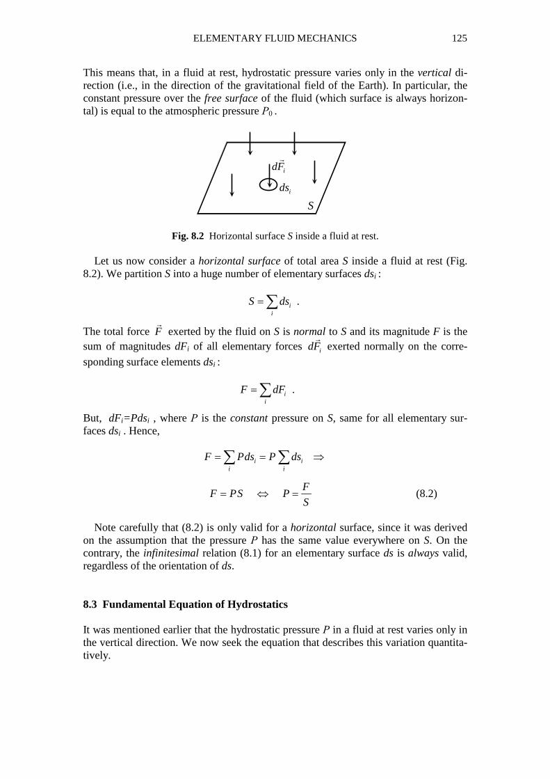
ELEMENTARY FLUID MECHANICS 125
This means that, in a fluid at rest, hydrostatic pressure varies only in the vertical di-rection (i.e., in the direction of the gravitational field of the Earth). In particular, the constant pressure over the free surface of the fluid (which surface is always horizon-tal) is equal to the atmospheric pressure Ρ0 .
S
ids
idF�
Fig. 8.2 Horizontal surface S inside a fluid at rest. Let us now consider a horizontal surface of total area S inside a fluid at rest (Fig. 8.2). We partition S into a huge number of elementary surfaces dsi : i
i
S ds= ∑ .
The total force F�
exerted by the fluid on S is normal to S and its magnitude F is the sum of magnitudes dFi of all elementary forces idF
�
exerted normally on the corre-
sponding surface elements dsi : i
i
F dF= ∑ .
But, dFi=Pdsi , where Ρ is the constant pressure on S, same for all elementary sur-faces dsi . Hence,
i ii i
F Pds P ds= = ⇒∑ ∑
F
F PS PS
= ⇔ = (8.2)
Note carefully that (8.2) is only valid for a horizontal surface, since it was derived on the assumption that the pressure Ρ has the same value everywhere on S. On the contrary, the infinitesimal relation (8.1) for an elementary surface ds is always valid, regardless of the orientation of ds. 8.3 Fundamental Equation of Hydrostatics It was mentioned earlier that the hydrostatic pressure Ρ in a fluid at rest varies only in the vertical direction. We now seek the equation that describes this variation quantita-tively.
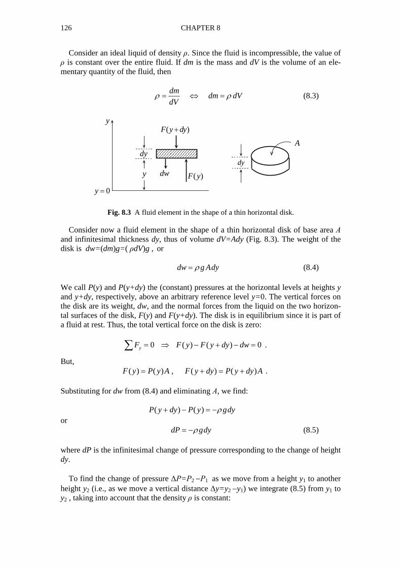
126 CHAPTER 8
Consider an ideal liquid of density ρ. Since the fluid is incompressible, the value of ρ is constant over the entire fluid. If dm is the mass and dV is the volume of an ele-mentary quantity of the fluid, then
dm
dm dVdV
ρ ρ= ⇔ = (8.3)
y
0y =
y
dy
dw ( )F y
( )F y dy+
dy
A
Fig. 8.3 A fluid element in the shape of a thin horizontal disk.
Consider now a fluid element in the shape of a thin horizontal disk of base area Α and infinitesimal thickness dy, thus of volume dV=Ady (Fig. 8.3). The weight of the disk is dw=(dm)g=( ρdV)g , or dw g Adyρ= (8.4) We call P(y) and P(y+dy) the (constant) pressures at the horizontal levels at heights y and y+dy, respectively, above an arbitrary reference level y=0. The vertical forces on the disk are its weight, dw, and the normal forces from the liquid on the two horizon-tal surfaces of the disk, F(y) and F(y+dy). The disk is in equilibrium since it is part of a fluid at rest. Thus, the total vertical force on the disk is zero: 0 ( ) ( ) 0yF F y F y dy dw= ⇒ − + − =∑ .
But, ( ) ( ) , ( ) ( )F y P y A F y dy P y dy A= + = + . Substituting for dw from (8.4) and eliminating Α, we find: ( ) ( )P y dy P y gdyρ+ − = − or dP gdyρ= − (8.5) where dP is the infinitesimal change of pressure corresponding to the change of height dy. To find the change of pressure ∆Ρ=Ρ2 −Ρ1 as we move from a height y1 to another height y2 (i.e., as we move a vertical distance ∆y=y2 −y1) we integrate (8.5) from y1 to y2 , taking into account that the density ρ is constant:
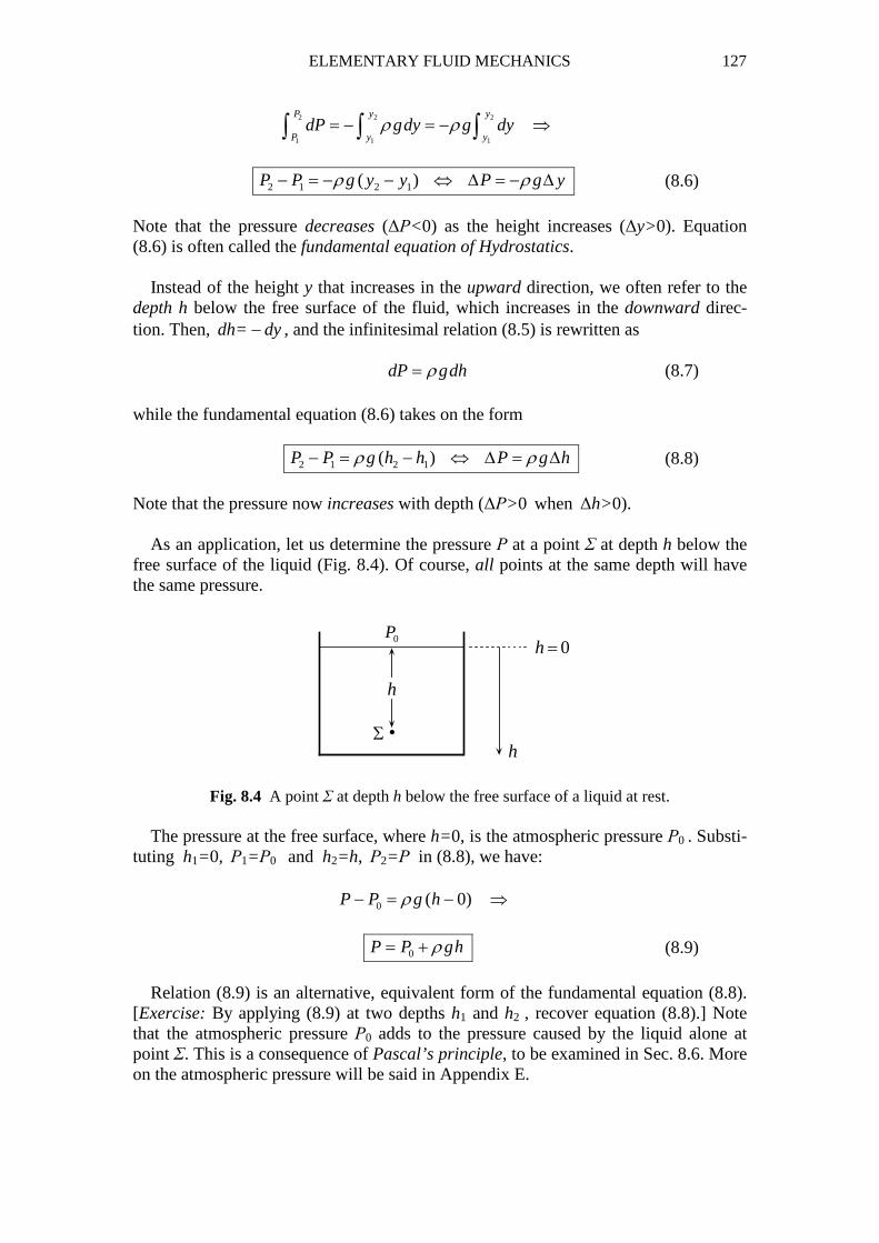
ELEMENTARY FLUID MECHANICS 127
2 2 2
1 1 1
P y y
P y ydP gdy g dyρ ρ= − = − ⇒∫ ∫ ∫
2 1 2 1( )P P g y y P g yρ ρ− = − − ⇔ ∆ = − ∆ (8.6)
Note that the pressure decreases (∆Ρ<0) as the height increases (∆y>0). Equation (8.6) is often called the fundamental equation of Hydrostatics. Instead of the height y that increases in the upward direction, we often refer to the depth h below the free surface of the fluid, which increases in the downward direc-tion. Then, dh= − dy , and the infinitesimal relation (8.5) is rewritten as dP gdhρ= (8.7) while the fundamental equation (8.6) takes on the form 2 1 2 1( )P P g h h P g hρ ρ− = − ⇔ ∆ = ∆ (8.8)
Note that the pressure now increases with depth (∆Ρ>0 when ∆h>0). As an application, let us determine the pressure Ρ at a point Σ at depth h below the free surface of the liquid (Fig. 8.4). Of course, all points at the same depth will have the same pressure.
h
hiΣ
0P0h =
Fig. 8.4 A point Σ at depth h below the free surface of a liquid at rest. The pressure at the free surface, where h=0, is the atmospheric pressure Ρ0 . Substi-tuting h1=0, Ρ1=Ρ0 and h2=h, Ρ2=Ρ in (8.8), we have: 0 ( 0)P P g hρ− = − ⇒
0P P ghρ= + (8.9)
Relation (8.9) is an alternative, equivalent form of the fundamental equation (8.8). [Exercise: By applying (8.9) at two depths h1 and h2 , recover equation (8.8).] Note that the atmospheric pressure Ρ0 adds to the pressure caused by the liquid alone at point Σ. This is a consequence of Pascal’s principle, to be examined in Sec. 8.6. More on the atmospheric pressure will be said in Appendix E.
128 CHAPTER 8
8.4 Units of Pressure Hydrostatic pressure is expressed in a variety of units, depending on the application of interest. The following units are commonly used in Physics. 1. In the S.I. system of units (m, kg, s) the unit of pressure is the Pascal (Pa):
2
1 1N
Pam
= where 21 1N kg m s−= ⋅ ⋅ .
In the cgs system (cm, g, s) the unit of pressure is
2
1dyn
cm where 21 1dyn g cm s−= ⋅ ⋅ .
Given that 1kg=103 g and that 1m=102 cm, we find that 1N=105 dyn, and therefore,
2
1 10dyn
Pacm
= .
2. The Bar unit is defined as follows:
6 52
1 10 10dyn
Bar Pacm
= = .
Hence,
62
1 10 1dyn
Bar Barcm
µ−= = .
3. As 1Torr or 1mmHg we define the pressure exerted at the base of a column of mercury (Hg) of height 1mm=0.1cm. Thus, 1Torr is the pressure change ∆Ρ that rela-tion (8.8) will yield by putting ρ=13.6 g/cm3 (density of Hg), g=9.8 m/s2 and ∆h=0.1cm :
3 2
2
1 (13.6 ) (980 ) (0.1 )
1332.8 1332.8 .
g cmTorr cm
cm sdyn
Barcm
µ
= × ×
= =
4. An atmosphere (1atm) is defined as the pressure exerted at the base of a column of Hg of height 76cm=760mm :
1 760 760 760 1332.8
1.01 .
atm mmHg Torr Bar
Bar
µ= = = ×
≃
This is equal to the standard atmospheric pressure P0 at sea level: 0 1 760P atm Torr= = (sea level, 20ο C ) .
Application: Variation of hydrostatic pressure inside the sea
It is known empirically that the hydrostatic pressure inside the sea increases ap-proximately by 1atm for every extra 10 meters of depth. This can be verified numeri-
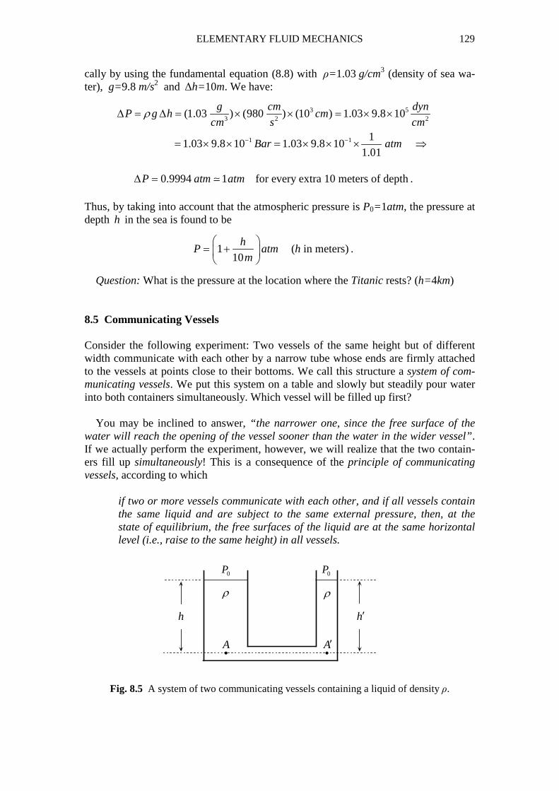
ELEMENTARY FLUID MECHANICS 129
cally by using the fundamental equation (8.8) with ρ=1.03 g/cm3 (density of sea wa-ter), g=9.8 m/s2 and ∆h=10m. We have:
3 53 2 2
1 1
(1.03 ) (980 ) (10 ) 1.03 9.8 10
11.03 9.8 10 1.03 9.8 10
1.01
g cm dynP g h cm
cm s cm
Bar atm
ρ
− −
∆ = ∆ = × × = × ×
= × × = × × × ⇒
0.9994 1P atm atm∆ = ≃ for every extra 10 meters of depth . Thus, by taking into account that the atmospheric pressure is P0=1atm, the pressure at depth h in the sea is found to be
110
hP atm
m
= +
(h in meters) .
Question: What is the pressure at the location where the Titanic rests? (h=4km) 8.5 Communicating Vessels Consider the following experiment: Two vessels of the same height but of different width communicate with each other by a narrow tube whose ends are firmly attached to the vessels at points close to their bottoms. We call this structure a system of com-municating vessels. We put this system on a table and slowly but steadily pour water into both containers simultaneously. Which vessel will be filled up first? You may be inclined to answer, “the narrower one, since the free surface of the water will reach the opening of the vessel sooner than the water in the wider vessel”. If we actually perform the experiment, however, we will realize that the two contain-ers fill up simultaneously! This is a consequence of the principle of communicating vessels, according to which
if two or more vessels communicate with each other, and if all vessels contain the same liquid and are subject to the same external pressure, then, at the state of equilibrium, the free surfaces of the liquid are at the same horizontal level (i.e., raise to the same height) in all vessels.
i i
ρ ρ
h h′
A A′
0P 0P
Fig. 8.5 A system of two communicating vessels containing a liquid of density ρ.

130 CHAPTER 8
The theoretical proof of the principle is as follows (see Fig. 8.5; for convenience, only two vessels are drawn). Consider two points Α and Α΄ located at different vessels but belonging to the same horizontal plane. The hydrostatic pressure is thus the same at the two points. Call h and h the heights of the free surfaces of the liquid above Α and Α΄, respectively. By relation (8.9), 0 0A AP P P gh P gh h hρ ρ ′ ′= ⇒ + = + ⇒ = .
Notice that the validity of this result is independent of the geometrical characteristics of the vessels. There are two cases where the principle of communicating vessels does not apply; namely, (a) when the vessels contain two or more liquids that do not mix, and (b) when the external pressures on the free surfaces of the contained liquid are different in different vessels. Let us see two examples: a. Vessels containing immiscible liquids of different densities
i i
A A′
0P 0P
i i
B B′
1ρ2ρ
1h 2h
interface
Fig. 8.6 A system of communicating vessels containing two liquids that do not mix.
The two vessels in Fig. 8.6 contain liquids of densities ρ1 and ρ2 , where we assume that ρ1 > ρ2 . We call h1 and h2 the heights of the free surfaces of the two liquids rela-tive to the horizontal level of their interface (the existence of such an interface is re-lated to the fact that the liquids do not mix). We consider the points Α and Α΄ belong-ing to the same horizontal plane within the liquid ρ1. We also consider the point Β in the liquid ρ1 , at the same horizontal level with the point Β΄ at the interface of the two liquids. Since Α and Α΄ are points in the same liquid, the hydrostatic pressures at these points are equal. By the fundamental equation (8.8),
1 1
1 1
( ) ( ) ,
( ) ( ) .A B A B
A΄ B΄ A΄ B΄
P P g AB P P g AB
P P g AB΄ P P g AB΄
ρ ρ
ρ ρ
− = ⇒ = +
− = ⇒ = +
Given that ΡΑ = ΡΑ΄ and ΑΒ=Α΄Β΄, we conclude that ΡΒ = ΡΒ΄ . Relation (8.9), then, yields:
0 1 1 0 2 2 1 1 2 2P g h P g h h hρ ρ ρ ρ+ = + ⇒ = ⇒
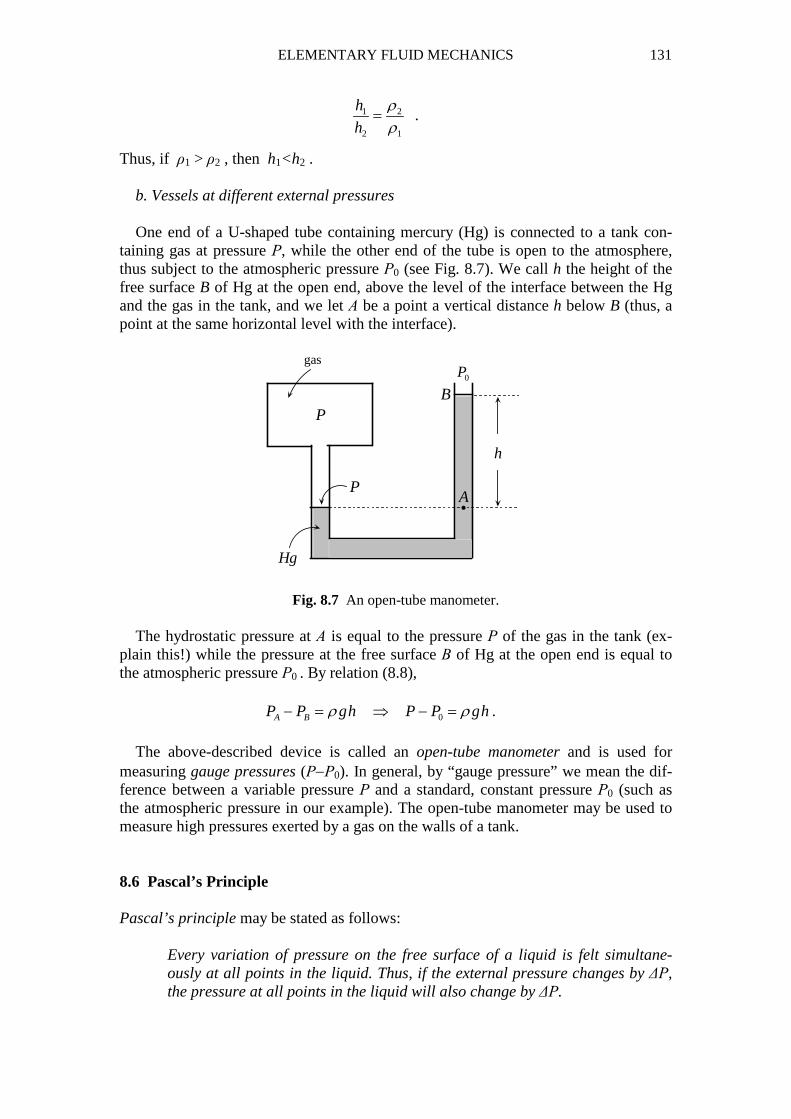
ELEMENTARY FLUID MECHANICS 131
1 2
2 1
h
h
ρρ
= .
Thus, if ρ1 > ρ2 , then h1<h2 . b. Vessels at different external pressures One end of a U-shaped tube containing mercury (Hg) is connected to a tank con-taining gas at pressure Ρ, while the other end of the tube is open to the atmosphere, thus subject to the atmospheric pressure Ρ0 (see Fig. 8.7). We call h the height of the free surface B of Hg at the open end, above the level of the interface between the Hg and the gas in the tank, and we let Α be a point a vertical distance h below B (thus, a point at the same horizontal level with the interface).
P
i
0P
h
A
B
P
Hg
gas
Fig. 8.7 An open-tube manometer. The hydrostatic pressure at Α is equal to the pressure Ρ of the gas in the tank (ex-plain this!) while the pressure at the free surface Β of Hg at the open end is equal to the atmospheric pressure Ρ0 . By relation (8.8), 0A BP P gh P P ghρ ρ− = ⇒ − = .
The above-described device is called an open-tube manometer and is used for measuring gauge pressures (Ρ−Ρ0). In general, by “gauge pressure” we mean the dif-ference between a variable pressure Ρ and a standard, constant pressure Ρ0 (such as the atmospheric pressure in our example). The open-tube manometer may be used to measure high pressures exerted by a gas on the walls of a tank. 8.6 Pascal’s Principle Pascal’s principle may be stated as follows:
Every variation of pressure on the free surface of a liquid is felt simultane-ously at all points in the liquid. Thus, if the external pressure changes by ∆Ρ, the pressure at all points in the liquid will also change by ∆Ρ.

132 CHAPTER 8
Proof: When the external pressure is Ρ0 , the pressure at a point Σ at depth h below the free surface of the liquid is Ρ=Ρ0+ρgh. If the external pressure increases by ∆Ρ, so that its new value is Ρ0΄=Ρ0+∆Ρ, the pressure at Σ will become Ρ΄ = Ρ0΄ + ρgh = (Ρ0+∆Ρ) + ρgh = (Ρ0 + ρgh) + ∆Ρ = Ρ +∆Ρ . Pascal’s principle has a useful practical application in the hydraulic lever. In its simplest form, this consists of two communicating cylindrical vessels of cross-sectional areas S1 and S2, where S1< S2 (see Fig. 8.8). The vessels contain a fluid such as oil or water. At the top of each cylinder there is a piston by which pressure can be exerted on the fluid at both sides. Assume now that we exert a downward force F1 on the smaller piston. What force F2 must be applied to the larger piston in order for the system to be in balance?
1S 2S
1F2F
2F ′
Fig. 8.8 A simplified form of a hydraulic lever.
The smaller piston exerts a pressure Ρ=F1 / S1 on the fluid. According to Pascal’s principle, this pressure is transferred to the larger piston, to which is thus exerted an upward force equal to
12 2 2
1
FF PS S
S′ = = .
In order for that piston to be in balance we must therefore exert on it a downward force of magnitude F2=F2΄ ; that is,
22 1
1
SF F
S= (8.10)
We notice that F2>F1. Thus, by a small effort (force F1) we can, e.g., lift a heavy ob-ject such as an automobile (force F2). 8.7 Archimedes’ Principle Archimedes’ principle is among the most important principles of Hydrostatics. It is stated as follows:
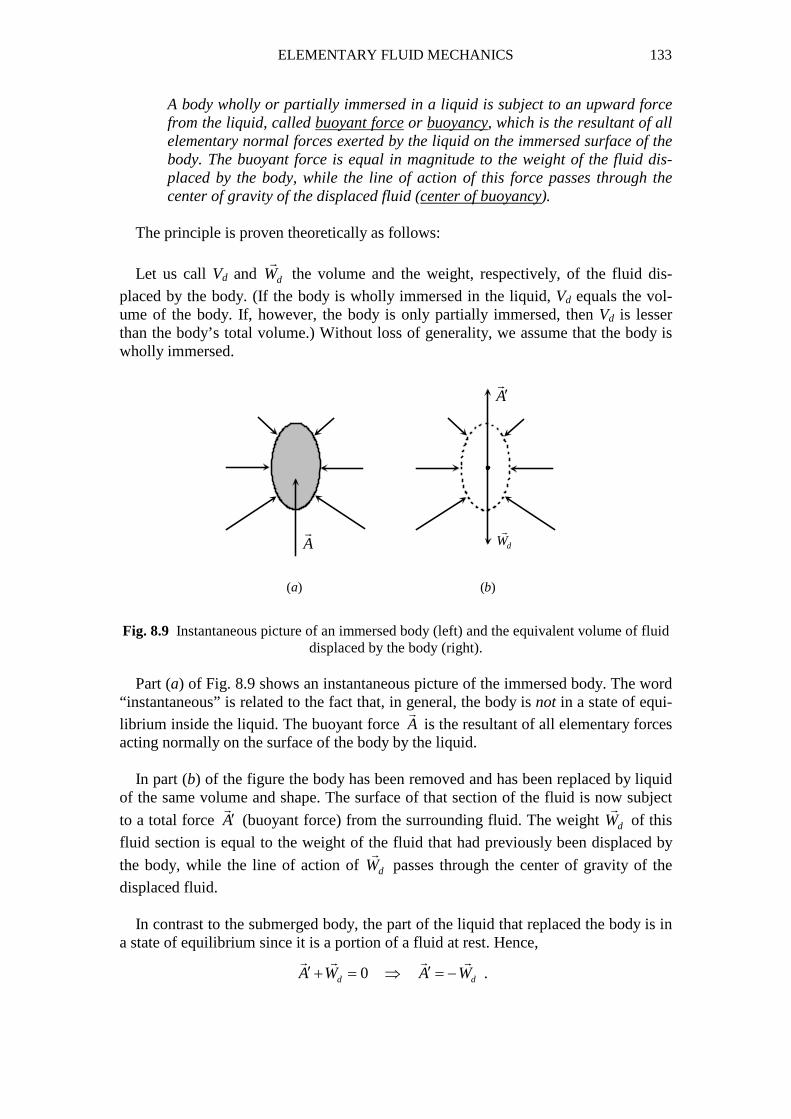
ELEMENTARY FLUID MECHANICS 133
A body wholly or partially immersed in a liquid is subject to an upward force from the liquid, called buoyant force or buoyancy, which is the resultant of all elementary normal forces exerted by the liquid on the immersed surface of the body. The buoyant force is equal in magnitude to the weight of the fluid dis-placed by the body, while the line of action of this force passes through the center of gravity of the displaced fluid (center of buoyancy).
The principle is proven theoretically as follows:
Let us call Vd and dW�
the volume and the weight, respectively, of the fluid dis-
placed by the body. (If the body is wholly immersed in the liquid, Vd equals the vol-ume of the body. If, however, the body is only partially immersed, then Vd is lesser than the body’s total volume.) Without loss of generality, we assume that the body is wholly immersed.
A�
A′�
dW�
( )a ( )b
Fig. 8.9 Instantaneous picture of an immersed body (left) and the equivalent volume of fluid
displaced by the body (right). Part (a) of Fig. 8.9 shows an instantaneous picture of the immersed body. The word “instantaneous” is related to the fact that, in general, the body is not in a state of equi-librium inside the liquid. The buoyant force A
�
is the resultant of all elementary forces acting normally on the surface of the body by the liquid. In part (b) of the figure the body has been removed and has been replaced by liquid of the same volume and shape. The surface of that section of the fluid is now subject
to a total force A′�
(buoyant force) from the surrounding fluid. The weight dW�
of this
fluid section is equal to the weight of the fluid that had previously been displaced by
the body, while the line of action of dW�
passes through the center of gravity of the
displaced fluid. In contrast to the submerged body, the part of the liquid that replaced the body is in a state of equilibrium since it is a portion of a fluid at rest. Hence,
0d dA W A W′ ′+ = ⇒ = −� �� �
.
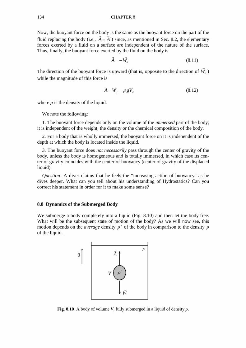
134 CHAPTER 8
Now, the buoyant force on the body is the same as the buoyant force on the part of the fluid replacing the body (i.e., A A′=
� �
) since, as mentioned in Sec. 8.2, the elementary forces exerted by a fluid on a surface are independent of the nature of the surface. Thus, finally, the buoyant force exerted by the fluid on the body is
dA W= −� �
(8.11)
The direction of the buoyant force is upward (that is, opposite to the direction of dW�
)
while the magnitude of this force is d dA W gVρ= = (8.12)
where ρ is the density of the liquid. We note the following:
1. The buoyant force depends only on the volume of the immersed part of the body; it is independent of the weight, the density or the chemical composition of the body.
2. For a body that is wholly immersed, the buoyant force on it is independent of the depth at which the body is located inside the liquid.
3. The buoyant force does not necessarily pass through the center of gravity of the body, unless the body is homogeneous and is totally immersed, in which case its cen-ter of gravity coincides with the center of buoyancy (center of gravity of the displaced liquid).
Question: A diver claims that he feels the “increasing action of buoyancy” as he dives deeper. What can you tell about his understanding of Hydrostatics? Can you correct his statement in order for it to make some sense? 8.8 Dynamics of the Submerged Body We submerge a body completely into a liquid (Fig. 8.10) and then let the body free. What will be the subsequent state of motion of the body? As we will now see, this motion depends on the average density ρ΄ of the body in comparison to the density ρ of the liquid.
u
V
ρ
ρ ′
A�
W�
Fig. 8.10 A body of volume V, fully submerged in a liquid of density ρ.
ELEMENTARY FLUID MECHANICS 135
Let m, V, W be the mass, the volume and the weight, respectively, of the submerged body. The average density of the body is defined as
m
m VV
ρ ρ′ ′= ⇔ = (8.13)
Hence,
W mg gVρ ′= = (8.14)
Since the body is fully immersed, Vd =V, where Vd is the volume of the fluid dis-placed by the body. By (8.12), then, the buoyant force on the body has magnitude
A gVρ= .
In vector form, by taking the positive direction (defined by the direction of the unit vector u in Fig. 8.10) upward, we have:
ˆ ˆ ˆ ˆ,A A u gV u W W u gV uρ ρ ′= = = − = −� �
.
The total force on the body is
ˆ ˆ ˆ( ) ( )F A W A W u gV u F uρ ρ ′= + = − = − ≡�� �
.
Note that the direction of F�
depends on the sign of the algebraic value
( )F A W gVρ ρ ′= − = − (8.15)
Specifically:
• If ρ΄ > ρ , then F < 0 and the body sinks.
• If ρ΄ = ρ , then F = 0 and the body attains a state of equilibrium, fully sub-merged in the liquid.
• If ρ΄ < ρ , then F > 0 and the body rises toward the surface of the liquid and finally floats in equilibrium, partially submerged in the fluid.
The average density ρ΄ of a submarine can be varied with the inflow or outflow of seawater, thus becoming larger, smaller or equal to the density ρ of the water. In this way one can achieve diving, surfacing or equilibrium, respectively, of the submarine in the water. 8.9 Equilibrium of a Floating Body As we have seen, for a body to float partially submerged in a liquid (as shown in Fig. 8.11) the average density ρ΄ of the body must be smaller than the density ρ of the liq-uid (ρ΄< ρ). We call V and W the volume and the weight, respectively, of the body, and we let Vd be the volume of the immersed part of the body, equal to the volume of the displaced liquid. In addition to its weight W, the body is subject to the buoyant force Α exerted by the fluid on the immersed surface of the body. We want to evaluate the fraction of the total volume of the body that is submerged.
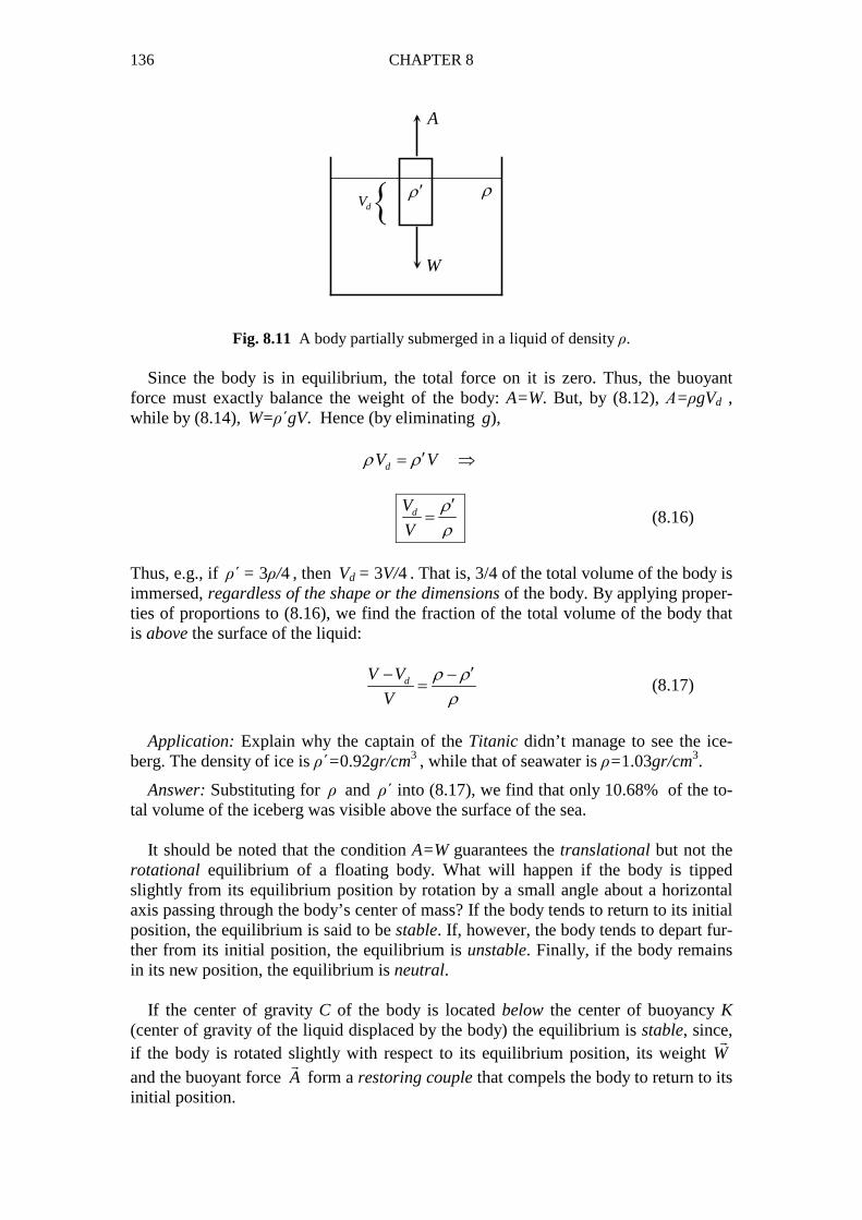
136 CHAPTER 8
A
W
ρρ ′{dV
Fig. 8.11 A body partially submerged in a liquid of density ρ.
Since the body is in equilibrium, the total force on it is zero. Thus, the buoyant force must exactly balance the weight of the body: A=W. But, by (8.12), Α=ρgVd , while by (8.14), W=ρ΄gV. Hence (by eliminating g), dV Vρ ρ ′= ⇒
dV
V
ρρ
′= (8.16)
Thus, e.g., if ρ΄ = 3ρ/4 , then Vd = 3V/4 . That is, 3/4 of the total volume of the body is immersed, regardless of the shape or the dimensions of the body. By applying proper-ties of proportions to (8.16), we find the fraction of the total volume of the body that is above the surface of the liquid:
dV V
V
ρ ρρ
′− −= (8.17)
Application: Explain why the captain of the Titanic didn’t manage to see the ice-berg. The density of ice is ρ΄=0.92gr/cm3
, while that of seawater is ρ=1.03gr/cm3.
Answer: Substituting for ρ and ρ΄ into (8.17), we find that only 10.68% of the to-tal volume of the iceberg was visible above the surface of the sea. It should be noted that the condition A=W guarantees the translational but not the rotational equilibrium of a floating body. What will happen if the body is tipped slightly from its equilibrium position by rotation by a small angle about a horizontal axis passing through the body’s center of mass? If the body tends to return to its initial position, the equilibrium is said to be stable. If, however, the body tends to depart fur-ther from its initial position, the equilibrium is unstable. Finally, if the body remains in its new position, the equilibrium is neutral. If the center of gravity C of the body is located below the center of buoyancy K (center of gravity of the liquid displaced by the body) the equilibrium is stable, since, if the body is rotated slightly with respect to its equilibrium position, its weight W
�
and the buoyant force A
�
form a restoring couple that compels the body to return to its initial position.
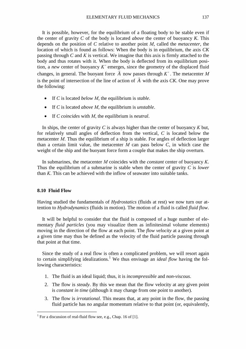
ELEMENTARY FLUID MECHANICS 137
It is possible, however, for the equilibrium of a floating body to be stable even if the center of gravity C of the body is located above the center of buoyancy K. This depends on the position of C relative to another point Μ, called the metacenter, the location of which is found as follows: When the body is in equilibrium, the axis CK passing through C and Κ is vertical. We imagine that this axis is firmly attached to the body and thus rotates with it. When the body is deflected from its equilibrium posi-tion, a new center of buoyancy Κ΄ emerges, since the geometry of the displaced fluid changes, in general. The buoyant force A
�
now passes through Κ΄ . The metacenter Μ
is the point of intersection of the line of action of A�
with the axis CK. One may prove the following:
• If C is located below Μ, the equilibrium is stable.
• If C is located above Μ, the equilibrium is unstable.
• If C coincides with Μ, the equilibrium is neutral. In ships, the center of gravity C is always higher than the center of buoyancy Κ but, for relatively small angles of deflection from the vertical, C is located below the metacenter Μ. Thus the equilibrium of a ship is stable. For angles of deflection larger than a certain limit value, the metacenter Μ can pass below C, in which case the weight of the ship and the buoyant force form a couple that makes the ship overturn. In submarines, the metacenter Μ coincides with the constant center of buoyancy Κ. Thus the equilibrium of a submarine is stable when the center of gravity C is lower than Κ. This can be achieved with the inflow of seawater into suitable tanks. 8.10 Fluid Flow Having studied the fundamentals of Hydrostatics (fluids at rest) we now turn our at-tention to Hydrodynamics (fluids in motion). The motion of a fluid is called fluid flow. It will be helpful to consider that the fluid is composed of a huge number of ele-mentary fluid particles (you may visualize them as infinitesimal volume elements) moving in the direction of the flow at each point. The flow velocity at a given point at a given time may thus be defined as the velocity of the fluid particle passing through that point at that time. Since the study of a real flow is often a complicated problem, we will resort again to certain simplifying idealizations.1 We thus envisage an ideal flow having the fol-lowing characteristics:
1. The fluid is an ideal liquid; thus, it is incompressible and non-viscous.
2. The flow is steady. By this we mean that the flow velocity at any given point is constant in time (although it may change from one point to another).
3. The flow is irrotational. This means that, at any point in the flow, the passing fluid particle has no angular momentum relative to that point (or, equivalently,
1 For a discussion of real-fluid flow see, e.g., Chap. 16 of [1].
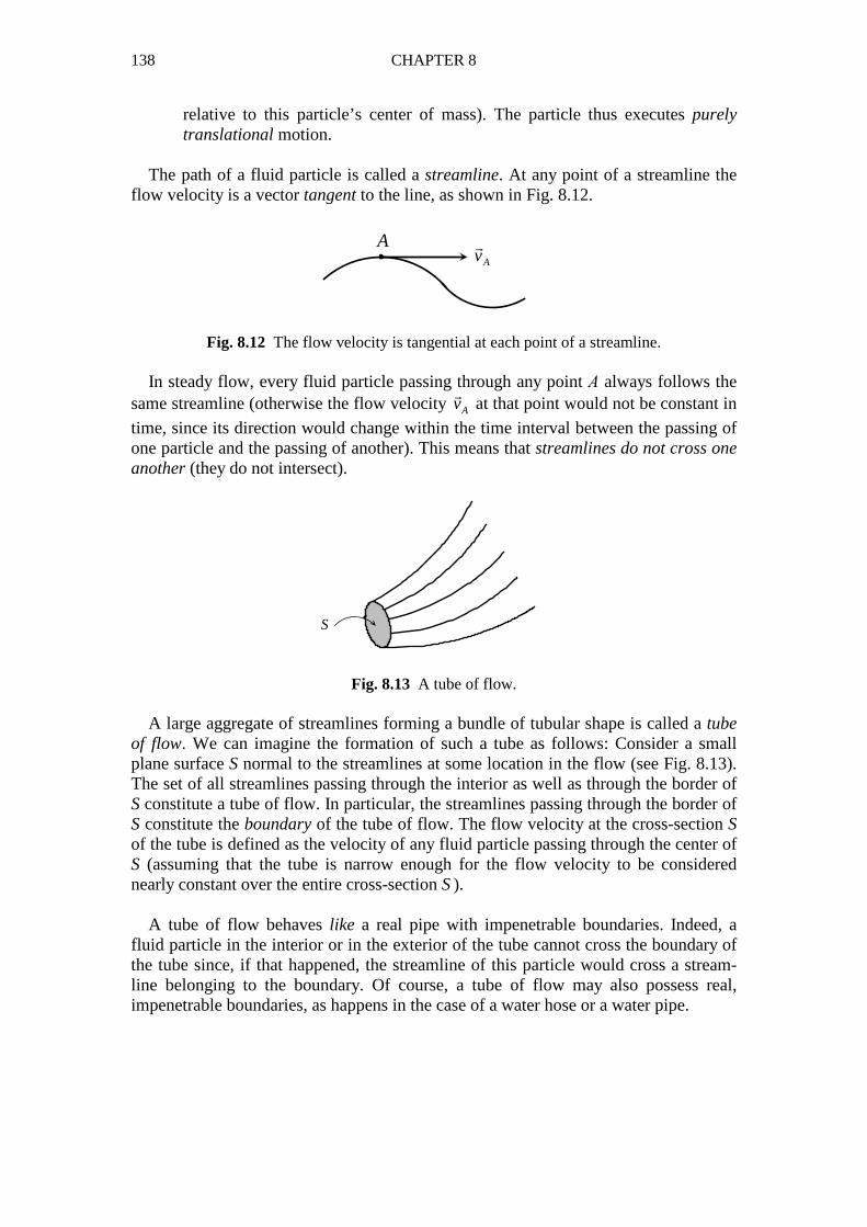
138 CHAPTER 8
relative to this particle’s center of mass). The particle thus executes purely translational motion.
The path of a fluid particle is called a streamline. At any point of a streamline the flow velocity is a vector tangent to the line, as shown in Fig. 8.12.
AAv�
Fig. 8.12 The flow velocity is tangential at each point of a streamline. In steady flow, every fluid particle passing through any point Α always follows the same streamline (otherwise the flow velocity Av
�
at that point would not be constant in
time, since its direction would change within the time interval between the passing of one particle and the passing of another). This means that streamlines do not cross one another (they do not intersect).
S
Fig. 8.13 A tube of flow. A large aggregate of streamlines forming a bundle of tubular shape is called a tube of flow. We can imagine the formation of such a tube as follows: Consider a small plane surface S normal to the streamlines at some location in the flow (see Fig. 8.13). The set of all streamlines passing through the interior as well as through the border of S constitute a tube of flow. In particular, the streamlines passing through the border of S constitute the boundary of the tube of flow. The flow velocity at the cross-section S of the tube is defined as the velocity of any fluid particle passing through the center of S (assuming that the tube is narrow enough for the flow velocity to be considered nearly constant over the entire cross-section S ). A tube of flow behaves like a real pipe with impenetrable boundaries. Indeed, a fluid particle in the interior or in the exterior of the tube cannot cross the boundary of the tube since, if that happened, the streamline of this particle would cross a stream-line belonging to the boundary. Of course, a tube of flow may also possess real, impenetrable boundaries, as happens in the case of a water hose or a water pipe.
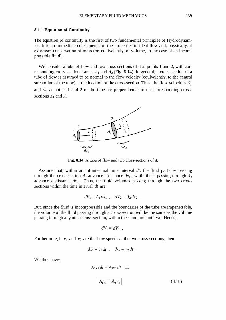
ELEMENTARY FLUID MECHANICS 139
8.11 Equation of Continuity The equation of continuity is the first of two fundamental principles of Hydrodynam-ics. It is an immediate consequence of the properties of ideal flow and, physically, it expresses conservation of mass (or, equivalently, of volume, in the case of an incom-pressible fluid). We consider a tube of flow and two cross-sections of it at points 1 and 2, with cor-responding cross-sectional areas Α1 and Α2 (Fig. 8.14). In general, a cross-section of a tube of flow is assumed to be normal to the flow velocity (equivalently, to the central streamline of the tube) at the location of the cross-section. Thus, the flow velocities 1v
�
and 2v�
at points 1 and 2 of the tube are perpendicular to the corresponding cross-
sections Α1 and Α2 .
{{
1
2
1A2A1v
�
2v�
1dx2dx
Fig. 8.14 A tube of flow and two cross-sections of it. Assume that, within an infinitesimal time interval dt, the fluid particles passing through the cross-section Α1 advance a distance dx1 , while those passing through Α2 advance a distance dx2 . Thus, the fluid volumes passing through the two cross-sections within the time interval dt are dV1 = A1 dx1 , dV2 = A2 dx2 . But, since the fluid is incompressible and the boundaries of the tube are impenetrable, the volume of the fluid passing through a cross-section will be the same as the volume passing through any other cross-section, within the same time interval. Hence, dV1 = dV2 . Furthermore, if v1 and v2 are the flow speeds at the two cross-sections, then dx1 = v1 dt , dx2 = v2 dt . We thus have:
A1v1 dt = A2v2 dt ⇒
1 1 2 2A v A v= (8.18)
140 CHAPTER 8
Given that the points 1 and 2 of the tube are chosen arbitrarily, relation (8.18) is equivalently restated as follows: A v⋅ = constant along the tube of flow (8.19) Relations (8.18) and (8.19) are alternate versions of the equation of continuity for a tube of flow. Note that the proof of this equation was based on the assumption that the boundaries of the tube are impenetrable, which means that it is impossible for any quantity of fluid to either enter or exit the tube. This implies that the quantity of fluid passing through any cross-section of the tube per unit time must be the same for all cross-sections of the tube. The product A.v carries a particular physical significance, which becomes evident by noting that
dx dV
A v Adt dt
= =
where dV is the volume of fluid passing through the cross-section Α within time dt. Thus, the product A.v represents the fluid volume per unit time passing through the cross-section Α of the tube; it is called the volume flow rate (or volume flux):
Π = Α v = dV
dt = volume flow rate (8.20)
According to the equation of continuity (8.19), the flow rate is constant along the tube. That is, the same volume of fluid passes per unit time through every cross-section of the tube, in accordance with a remark made earlier. 8.12 Bernoulli’s Equation Bernoulli’s equation, to be proven in Appendix F, is an expression of conservation of mechanical energy for a fluid (here, a liquid). Specifically, it is the analog of relation (6.28) for the case of a mechanical system consisting of elementary fluid particles. Consider a tube of flow of a liquid of density ρ. Consider also two cross-sections of the tube, of areas Α1 and Α2 , at the corresponding points 1 and 2 of the tube (Fig. 8.15). The flow velocities, of magnitudes v1 and v2 , are normal to the corresponding cross-sections. We call Ρ1, Ρ2 the hydrostatic pressures at the two cross-sections, and we call y1, y2 the heights at which the centers of these cross-sections are located above an arbitrary reference level.

ELEMENTARY FLUID MECHANICS 141
1
2
1A2A1v
�
2v�
1P 2P1y
2y
y
0y =
Fig. 8.15 A tube of flow and two cross-sections at different heights above an
arbitrary reference level. To understand how the pressures Ρ1 and Ρ2 are defined, let us consider the section of the tube extending from point 1 to point 2. This section is bounded by the cross-sections Α1 and Α2 . Assuming that, at any point of the tube, the hydrostatic pressure is constant (or approximately constant) over the entire cross-section at that point, we write:
1 21 2
1 2
,F F
P PA A
= =
where F1, F2 are the forces exerted normally on the cross-sections Α1, Α2 , respec-tively, by the fluid surrounding the considered section of the tube. (These forces must be normal to the corresponding cross-sections, given that, in general, every cross-section of the tube moves in a direction perpendicular to itself.) According to Bernoulli’s equation, for any two points 1 and 2 of the tube of flow,
2 21 1 1 2 2 2
1 1
2 2P v g y P v g yρ ρ ρ ρ+ + = + + (8.21)
or, equivalently,
21
2P v g yρ ρ+ + = constant along the tube of flow (8.22)
If we overlook, for a moment, the presence of the pressure Ρ, the left-hand side of (8.22) looks like a total mechanical energy in the gravitational field of the Earth, ex-cept that in place of the mass m we now have the density ρ of the fluid. The quantity Ρ here is related to the work required to change this mechanical energy, according to relation (6.28). To be specific, in addition to being subject to the conservative force of gravity, the considered section of the tube is subject to the normal forces F1, F2 by the surrounding fluid. The work of these forces is represented by the term Ρ in Bernoulli’s equation. This work is responsible for the change of total mechanical energy of the section of the tube (for more details, see Appendix F).
142 CHAPTER 8
In the trivial case where the flow velocity is zero, the equations of Hydrodynamics must reduce to those of Hydrostatics. For a fluid at rest, we must put v1=v2=0 into Bernoulli’s equation (8.21). This equation then yields: 2 1 2 1( )P P g y yρ− = − − (8.23)
Relation (8.23) is precisely the fundamental equation (8.6) of Hydrostatics. 8.13 Horizontal Flow We say that a tube of flow is horizontal if the central streamline (which does not have to be rectilinear) lies on a horizontal plane. All cross-sections of a horizontal tube of flow are centered at the same height y above a horizontal reference level. Thus, by putting y1=y2 into Bernoulli’s equation (8.21) the y-dependent terms cancel out and the equation reduces to
2 21 1 2 2
1 1
2 2P v P vρ ρ+ = + (8.24)
or
21
2P vρ+ = constant (8.25)
For a fluid at rest (v=0) it follows from (8.25) that the hydrostatic pressure Ρ is constant along any horizontal path. This conclusion is in perfect agreement with Hy-drostatics. Things are different in Hydrodynamics, however, where v≠ 0. According to (8.25), in order for the pressure Ρ along a horizontal tube of flow to be constant, the flow speed v must be constant along the tube. On the other hand, by the equation of continuity, the product A.v is constant along the tube, where Α is the cross-sectional area of the tube. Hence Α must be constant as well. We conclude that
the hydrostatic pressure is constant along a horizontal tube of flow having a constant cross-sectional area.
According to (8.25), in horizontal flow the hydrostatic pressure Ρ increases where the flow speed v decreases. Now, according to the equation of continuity, the flow speed decreases where the cross-sectional area A of the tube increases. Therefore,
in a horizontal tube of flow the hydrostatic pressure increases (decreases) where the cross-sectional area of the tube increases (decreases).
As an application, consider a horizontal pipe of variable cross-sectional area Α (Fig. 8.16). Consider two points – say, 1 and 2 – of the pipe and let Α1 and Α2 be the cross-sectional areas of the pipe at these points, where Α1>Α2 . A liquid of density ρ flows in the pipe. The pressure difference (Ρ1–Ρ2) between the two points is measured and found equal to ∆Ρ. What is the volume flow rate of this horizontal flow?
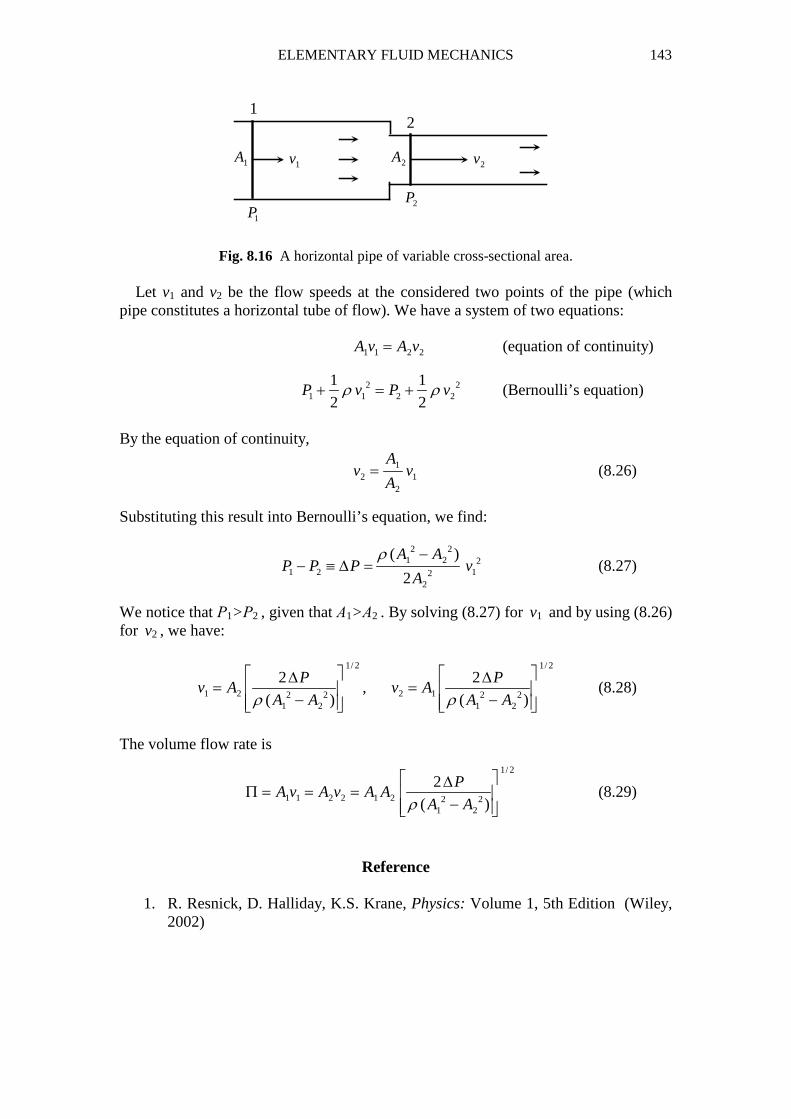
ELEMENTARY FLUID MECHANICS 143
12
1A 2A1v 2v
1P2P
Fig. 8.16 A horizontal pipe of variable cross-sectional area. Let v1 and v2 be the flow speeds at the considered two points of the pipe (which pipe constitutes a horizontal tube of flow). We have a system of two equations:
1 1 2 2A v A v= (equation of continuity)
2 21 1 2 2
1 1
2 2P v P vρ ρ+ = + (Bernoulli’s equation)
By the equation of continuity,
12 1
2
Av v
A= (8.26)
Substituting this result into Bernoulli’s equation, we find:
2 2
1 2 21 2 12
2
( )
2
A AP P P v
A
ρ −− ≡ ∆ = (8.27)
We notice that Ρ1>Ρ2 , given that Α1>Α2 . By solving (8.27) for v1 and by using (8.26) for v2 , we have:
1/ 2 1/ 2
1 2 2 12 2 2 21 2 1 2
2 2,
( ) ( )
P Pv A v A
A A A Aρ ρ
∆ ∆= =
− − (8.28)
The volume flow rate is
1/ 2
1 1 2 2 1 2 2 21 2
2
( )
PA v A v A A
A Aρ
∆Π = = =
− (8.29)
Reference
1. R. Resnick, D. Halliday, K.S. Krane, Physics: Volume 1, 5th Edition (Wiley, 2002)
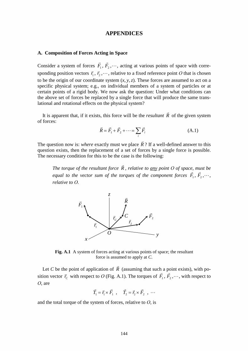
144
APPENDICES
A. Composition of Forces Acting in Space Consider a system of forces 1 2, ,F F
� �
⋯ , acting at various points of space with corre-
sponding position vectors 1 2, ,r r� �
⋯ , relative to a fixed reference point Ο that is chosen
to be the origin of our coordinate system (x, y, z). These forces are assumed to act on a specific physical system; e.g., on individual members of a system of particles or at certain points of a rigid body. We now ask the question: Under what conditions can the above set of forces be replaced by a single force that will produce the same trans-lational and rotational effects on the physical system? It is apparent that, if it exists, this force will be the resultant R
�
of the given system of forces:
1 2 ii
R F F F= + + =∑� � � �
⋯ (A.1)
The question now is: where exactly must we place R�
? If a well-defined answer to this question exists, then the replacement of a set of forces by a single force is possible. The necessary condition for this to be the case is the following:
The torque of the resultant force R�
, relative to any point Ο of space, must be
equal to the vector sum of the torques of the component forces 1 2, ,F F� �
⋯ ,
relative to Ο.
xy
z
O
C
1r� 2r
�Cr�
1F�
2F�
R�
Fig. A.1 A system of forces acting at various points of space; the resultant force is assumed to apply at C.
Let C be the point of application of R
�
(assuming that such a point exists), with po-
sition vector Cr�
with respect to Ο (Fig. A.1). The torques of 1 2, ,F F� �
⋯ , with respect to
Ο, are
1 1 1 2 2 2, ,T r F T r F= × = ×� � � �� �
⋯
and the total torque of the system of forces, relative to Ο, is
APPENDICES 145
1 2 i i ii i
T T T T r F= + + = = ×∑ ∑� � � � ��
⋯ (A.2)
On the other hand, the torque of R�
relative to Ο is
C C ii
r R r F× = × ∑� �� �
.
Thus, the necessary condition stated above is written:
C i i Ci i
r F T r R T× = ⇔ × =∑ ∑� � � �� �
(A.3)
The question then is whether the vector equation (A.3) has a solution for Cr�
, for given
R�
and T�
and for arbitrary choice of reference point Ο. A particular situation is that in which all forces iF
�
act at the same point Α, which
has position vector r�
. Then ir r=� �
, for all values of i, and
i i i ii i i
T r F r F r F r R= × = × = × = ×∑ ∑ ∑� � � � �� � � �
.
Hence, relation (A.3) has the solution Cr r=� �
. We conclude that
a system of forces that are concurrent at a point A may be replaced by their resultant, applied at the same point A .
Things aren’t that simple in the case of non-concurrent forces, since the equation (A.3) may not admit a solution for Cr
�
in that case. We can state, however, two neces-
sary conditions for the existence of such a solution:
1. The resultant force R�
must not be zero ( 0R ≠�
). Indeed, if the resultant is zero, equation (A.3) will either be impossible to solve for Cr
�
(if 0T ≠�
) or will
be indeterminate (if 0T =�
). For example, in the case of a couple F�
and F−�
(see Sec. 7.8) the vector Cr
�
is not defined, since 0R =�
while 0T ≠�
; hence the
solution of (A.3) is impossible.
2. The total torque T�
of the system, relative to any point O, must be normal to the resultant force R
�
. This follows from (A.3) and from the definition of the vector product.
We remark that, although the position vector Cr
�
of the point of application C of the
resultant force depends on the choice of the reference point Ο, the location of C rela-tive to the system of forces must be uniquely determined, independently of the choice of Ο. A case where all the above conditions are fulfilled is that of a system of parallel forces:
ˆ , 1,2,i iF F u i= =�
⋯ (A.4)
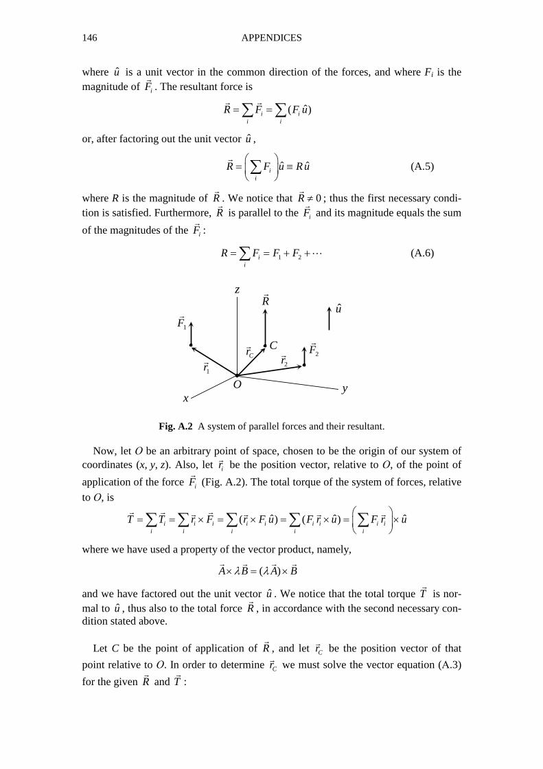
146 APPENDICES
where u is a unit vector in the common direction of the forces, and where Fi is the magnitude of iF
�
. The resultant force is
ˆ( )i ii i
R F F u= =∑ ∑� �
or, after factoring out the unit vector u ,
ˆ ˆii
R F u Ru
= ≡ ∑
�
(A.5)
where R is the magnitude of R�
. We notice that 0R ≠�
; thus the first necessary condi-tion is satisfied. Furthermore, R
�
is parallel to the iF�
and its magnitude equals the sum
of the magnitudes of the iF�
:
1 2ii
R F F F= = + +∑ ⋯ (A.6)
xy
z
O
C
1r� 2r
�Cr�
1F�
2F�
R�
u
Fig. A.2 A system of parallel forces and their resultant. Now, let Ο be an arbitrary point of space, chosen to be the origin of our system of coordinates (x, y, z). Also, let ir
�
be the position vector, relative to Ο, of the point of
application of the force iF�
(Fig. A.2). The total torque of the system of forces, relative
to Ο, is
ˆ ˆ ˆ( ) ( )i i i i i i i i ii i i i i
T T r F r F u F r u F r u
= = × = × = × = ×
∑ ∑ ∑ ∑ ∑� � �� � � �
where we have used a property of the vector product, namely,
( )A B A Bλ λ× = ×� �� �
and we have factored out the unit vector u . We notice that the total torque T�
is nor-mal to u , thus also to the total force R
�
, in accordance with the second necessary con-dition stated above. Let C be the point of application of R
�
, and let Cr�
be the position vector of that
point relative to Ο. In order to determine Cr�
we must solve the vector equation (Α.3)
for the given R�
and T�
:
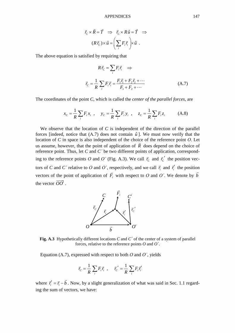
APPENDICES 147
ˆ
ˆ ˆ( ) .
C C
C i ii
r R T r Ru T
R r u F r u
× = ⇒ × = ⇒
× = ×
∑
� � �� �
� �
The above equation is satisfied by requiring that
C i ii
R r F r= ⇒∑� �
1 1 2 2
1 2
1C i i
i
F r F rr F r
R F F
+ += =
+ +∑� �
� � ⋯
⋯
(A.7)
The coordinates of the point C, which is called the center of the parallel forces, are
1 1 1
, ,C i i C i i C i ii i i
x F x y F y z F zR R R
= = =∑ ∑ ∑ (A.8)
We observe that the location of C is independent of the direction of the parallel forces [indeed, notice that (Α.7) does not contain u ]. We must now verify that the location of C in space is also independent of the choice of the reference point Ο. Let us assume, however, that the point of application of R
�
does depend on the choice of reference point. Thus, let C and C΄ be two different points of application, correspond-
ing to the reference points Ο and Ο΄ (Fig. A.3). We call Cr�
and Cr ′� the position vec-
tors of C and C΄ relative to Ο and Ο΄, respectively, and we call ir�
and ir ′� the position
vectors of the point of application of iF�
with respect to Ο and Ο΄. We denote by b�
the vector OO′�����
.
ii
O O′b�
C C′
ir�
ir ′� Cr ′�Cr�
iF�
Fig. A.3 Hypothetically different locations C and C of the center of a system of parallel forces, relative to the reference points O and O .
Equation (Α.7), expressed with respect to both Ο and Ο΄, yields
1 1
,C i i C i ii i
r F r r F rR R
′ ′= =∑ ∑� � � �
where i ir r b′ = −�
� �
. Now, by a slight generalization of what was said in Sec. 1.1 regard-
ing the sum of vectors, we have:
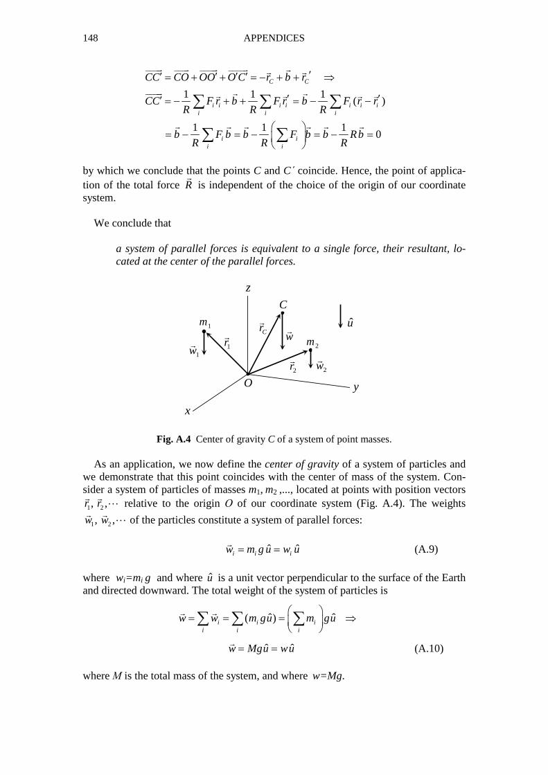
148 APPENDICES
1 1 1
( )
1 1 10
C C
i i i i i i ii i i
i ii i
CC CO OO O C r b r
CC F r b F r b F r rR R R
b F b b F b b RbR R R
′′ ′ ′ ′= + + = − + + ⇒
′ ′′ = − + + = − −
= − = − = − =
∑ ∑ ∑
∑ ∑
����� ���� ����� ����� �� �
����� � �� � � �
� � � � � �
by which we conclude that the points C and C΄ coincide. Hence, the point of applica-tion of the total force R
�
is independent of the choice of the origin of our coordinate system. We conclude that
a system of parallel forces is equivalent to a single force, their resultant, lo-cated at the center of the parallel forces.
x
y
z
O
C
1r�
2r�
Cr� u
1w�
2w�
w�
1m
2m
Fig. A.4 Center of gravity C of a system of point masses. As an application, we now define the center of gravity of a system of particles and we demonstrate that this point coincides with the center of mass of the system. Con-sider a system of particles of masses m1, m2 ,..., located at points with position vectors
1 2, ,r r� �
⋯ relative to the origin Ο of our coordinate system (Fig. A.4). The weights
1 2, ,w w� �
⋯ of the particles constitute a system of parallel forces:
ˆ ˆi i iw m g u w u= =
�
(A.9)
where wi=mi g and where u is a unit vector perpendicular to the surface of the Earth and directed downward. The total weight of the system of particles is
ˆ ˆ( )i i ii i i
w w m gu m gu
= = = ⇒
∑ ∑ ∑� �
ˆ ˆw Mgu wu= =�
(A.10) where Μ is the total mass of the system, and where w=Mg.
APPENDICES 149
The center of gravity of a system of particles is the center C of the parallel forces
iw�
; that is, the point of application of the total weight w�
of the system. (Note that the
location of this point does not have to coincide with that of a particle!) The position of C relative to Ο is found from equation (A.7) by setting Fi= wi and R= w :
1 1 1
C i i i i i ii i i
r w r m gr g m rw Mg Mg
= = = ⇒∑ ∑ ∑� � � �
1
C i ii
r m rM
= ∑� �
(A.11)
We observe that
the center of gravity of a system of particles coincides with the center of mass of the system
[see equation (6.2)]. As shown previously,
the location of this point with respect to the system of particles is uniquely de-termined; in particular, it does not depend on the choice of the origin of our coordinate system.
The Cartesian coordinates of the center of gravity (equivalently, of the center of mass) of the system are given by the algebraic equations
1 1 1
, ,C i i C i i C i ii i i
x m x y m y z m zM M M
= = =∑ ∑ ∑ (A.12)
150 APPENDICES
B. Some Theorems on the Center of Mass Consider a system of particles of masses mi (i= 1,2,...). The total mass of the system is 1 2 3 i
i
M m m m m= + + + = ∑⋯ (B.1)
The center of mass of the system is defined as the point C with position vector
1 1 2 2
1 1( )C i i
i
r m r m r m rM M
= + + = ∑� � � �
⋯ (B.2)
relative to the origin O of our coordinate system (see Fig. 6.1). Theorem 1. The location of C relative to the system of particles does not depend on the choice of the reference point Ο. Proof: See Appendix A. For a more direct proof, note first that equation (B.2) be-comes identical to (A.7) if we put Fi and R in place of mi and M, respectively; then, simply follow the discussion after equation (A.8). The total angular momentum of the system of particles mi at time t, relative to an arbitrary reference point O, is
( )i i i ii i
L L m r v= = ×∑ ∑� � � �
(B.3)
In particular, the total angular momentum relative to the center of mass C of the sys-tem is
( )i i ii
L m r v′ ′′ = ×∑� � �
(B.4)
where primed quantities are measured with respect to C. Theorem 2. The total angular momentum of the system, with respect to a point O, is the sum of the angular momentum relative to the center of mass (“spin angular mo-mentum”) and the angular momentum, relative to O, of a hypothetical particle of mass equal to the total mass of the system, moving with the center of mass (“orbital angu-lar momentum”). Proof: We have:
,i i C i i Cr r r v v v′ ′= + = +� � � � � �
.
Substituting these into (B.3), and using (B.1) and (B.4), we get:
( )C C i i C C i ii i
L L M r v m r v r m v ′ ′′= + × + × + × ∑ ∑
� � � � � � � �
.
APPENDICES 151
But, 0i im r′Σ =�
and 0i im v′Σ =�
, since these sums are proportional to the position
vector and the velocity, respectively, of the center of mass relative to itself. Thus, fi-nally,
( )C CL L M r v′= + ×� � � �
(B.5)
Now, suppose O is the origin of an inertial reference frame. Let iF�
be the external
force acting on mi at time t. The total external torque acting on the system at this time, relative to O, is given by
ext i ii
T r F= ×∑� ��
(B.6)
If we make the assumption that all internal forces in the system are central, then the following relation exists between the total angular momentum and the total external torque, both quantities measured with respect to O (see Sec. 6.3):
extdL
Tdt
=
�
�
(B.7)
Equation (B.7) is always valid relative to the origin O of an inertial frame. How about its validity relative to the center of mass C of the system? If C moves at con-stant velocity relative to O, then C is a proper choice of point of reference for the vec-tor relation (B.7). But, what if C is accelerating relative to O ? Theorem 3. Equation (B.7) is always valid with respect to the center of mass C, even if C is accelerating relative to an inertial frame of reference. Proof: By differentiating (B.5) with respect to time, by using (B.7) and (B.6), and
by taking into account that the total external force on the system is ext CF M a=� �
(see
Sec. 6.2), we have:
( )( ) ( ) , which vanishesC C C CdL dL
M r a M v vdt dt
′= + × + × ⇒
� �
� � � �
ext ext( )i i Ci
dLT r F r F
dt
′≡ × = + × ⇒∑
�
� � �� �
ext
( )i i C i i C ii i i
i ii
dLr F r F r r F
dt
r F T
′= × − × = − ×
′ ′= × =
∑ ∑ ∑
∑
�
� � �� � � �
� ��
where extT ′�
is the total external torque with respect to the center of mass.
The above theorem justifies using (B.7) to analyze the motion of a rolling body on an inclined plane, even though the axis of rotation passes through the accelerating center of mass of the body.
152 APPENDICES
The total kinetic energy of the system of particles, relative to an external observer O, is
21
2k i ii
E m v= ∑ (B.8)
The total kinetic energy with respect to the center of mass C is
21
2k i ii
E m v′ ′= ∑ (B.9)
where, as before, primed quantities are measured relative to C. Theorem 4. The total kinetic energy of the system, relative to an observer O, is the sum of the kinetic energy relative to the center of mass and the kinetic energy, relative to O, of a hypothetical particle of mass equal to the total mass of the system, moving with the center of mass. Proof: We have:
2 2 2 2i i C i i i i C i Cv v v v v v v v v v′ ′ ′= + ⇒ = ⋅ = + + ⋅� � � � � � �
.
Substituting this into (B.8), and using (B.1) and (B.9), we get:
21
2k k C i i Ci
E E M v m v v ′ ′= + + ⋅ ∑ � �
.
But, as noted previously, the sum in the last term vanishes, being proportional to the velocity of the center of mass relative to itself. Thus, finally,
21
2k k CE E M v′= + (B.10)
Theorem 5.
(a) Consider a system of N particles of masses m1 , m2 , ... , mN . Let C be the center of mass of the system. If a new particle, of mass m , is placed at C, the center of mass of the enlarged system of (N+1) particles will still be at C.
(b) Consider a system of N particles of masses m1 , m2 , ... , mN . It is assumed that the location of one of the particles, say of mN , coincides with the center of mass C of the system. If we now remove this particle from the system, the center of mass of the remaining system of (N–1) particles will still be at C. Proof:
(a) The total mass of the original system of N particles is M=m1+m2+...+mN . The center of mass of this system is located at the point C with position vector
1 1 2 21
( )C N Nr m r m r m rM
= + + +� � � �
⋯
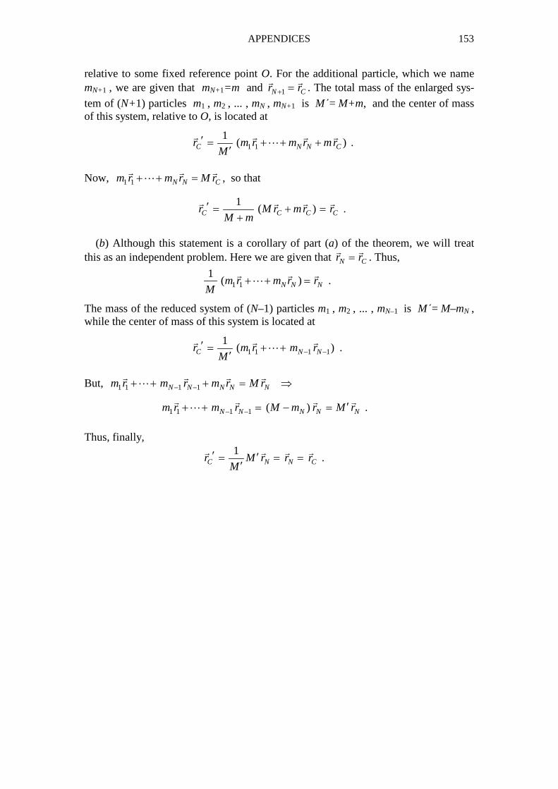
APPENDICES 153
relative to some fixed reference point O. For the additional particle, which we name mN+1 , we are given that mN+1=m and 1N Cr r+ =
� �
. The total mass of the enlarged sys-
tem of (N+1) particles m1 , m2 , ... , mN , mN+1 is M΄= M+m, and the center of mass of this system, relative to O, is located at
1 11
( )C N N Cr m r m r mrM
′ = + + +′
� � � �
⋯ .
Now, 1 1 N N Cm r m r M r+ + =� � �
⋯ , so that
1
( )C C C Cr M r mr rM m
′ = + =+
� � � �
.
(b) Although this statement is a corollary of part (a) of the theorem, we will treat this as an independent problem. Here we are given that N Cr r=
� �
. Thus,
1 11
( )N N Nm r m r rM
+ + =� � �
⋯ .
The mass of the reduced system of (N–1) particles m1 , m2 , ... , mN–1 is M΄= M–mN , while the center of mass of this system is located at
1 1 1 11
( )C N Nr m r m rM − −
′ = + +′
� � �
⋯ .
But, 1 1 1 1N N N N Nm r m r m r M r− −+ + + = ⇒� � � �
⋯
1 1 1 1 ( )N N N N Nm r m r M m r M r− − ′+ + = − =� � � �
⋯ .
Thus, finally,
1
C N N Cr M r r rM
′ ′= = =′
� � � �
.
154 APPENDICES
C. Table of Moments of Inertia1
Solid cylinder of radius R, relative to its axis: 21
2I MR=
Cylindrical shell of radius R, relative to its axis: 2I MR=
Circular disk of radius R, relative to a normal axis through
its center: 21
2I MR=
Ring of radius R, relative to a normal axis through its center: 2I MR=
Solid sphere of radius R, relative to an axis through its center: 22
5I MR=
Spherical shell of radius R, relative to an axis through its center: 22
3I MR=
Thin rod of length l, relative to a normal axis through
its center: 21
12I M l=
Thin rod of length l, relative to a normal axis through one
end (not a principal axis): 21
3I M l=
1 By M we denote the mass of the rigid body.
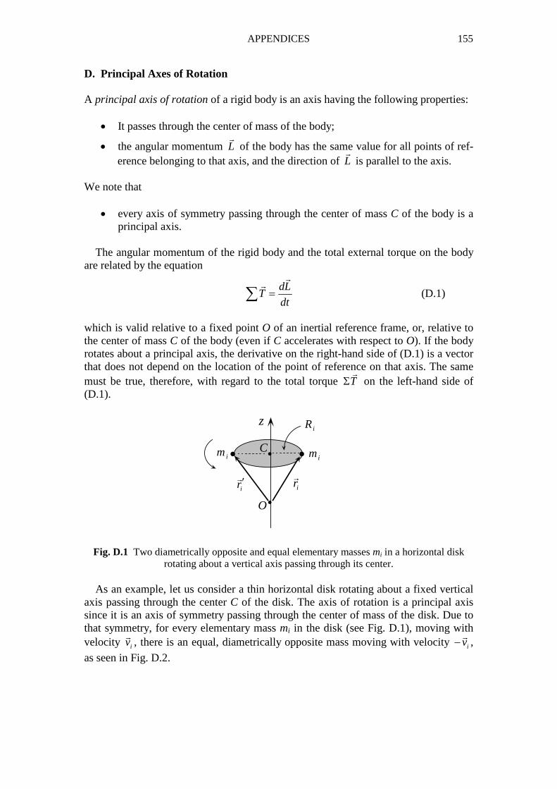
APPENDICES 155
D. Principal Axes of Rotation A principal axis of rotation of a rigid body is an axis having the following properties:
• It passes through the center of mass of the body;
• the angular momentum L�
of the body has the same value for all points of ref-erence belonging to that axis, and the direction of L
�
is parallel to the axis. We note that
• every axis of symmetry passing through the center of mass C of the body is a principal axis.
The angular momentum of the rigid body and the total external torque on the body are related by the equation
dL
Tdt
=∑�
�
(D.1)
which is valid relative to a fixed point O of an inertial reference frame, or, relative to the center of mass C of the body (even if C accelerates with respect to O). If the body rotates about a principal axis, the derivative on the right-hand side of (D.1) is a vector that does not depend on the location of the point of reference on that axis. The same must be true, therefore, with regard to the total torque TΣ
�
on the left-hand side of (D.1).
•
•
O
C •• imim
z
ir�
ir ′�
iR
Fig. D.1 Two diametrically opposite and equal elementary masses mi in a horizontal disk rotating about a vertical axis passing through its center.
As an example, let us consider a thin horizontal disk rotating about a fixed vertical axis passing through the center C of the disk. The axis of rotation is a principal axis since it is an axis of symmetry passing through the center of mass of the disk. Due to that symmetry, for every elementary mass mi in the disk (see Fig. D.1), moving with velocity iv
�
, there is an equal, diametrically opposite mass moving with velocity iv−�
,
as seen in Fig. D.2.
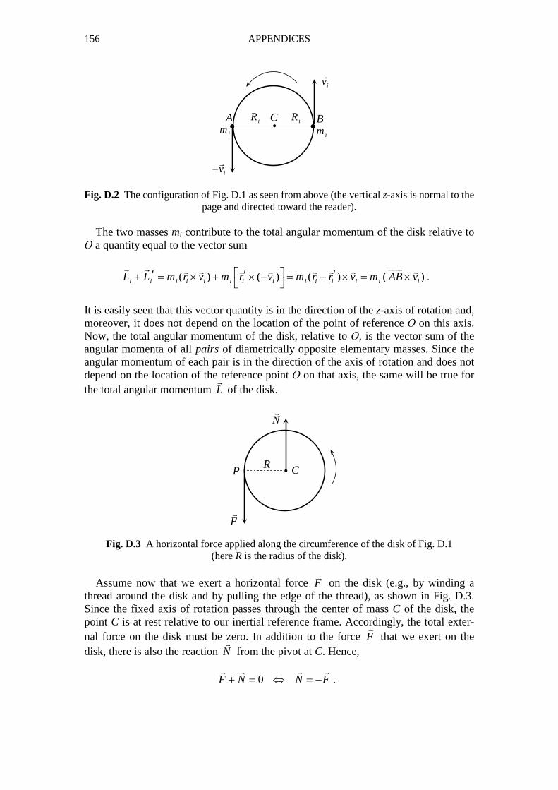
156 APPENDICES
i• •imim
C iRiR
iv�
iv−�
A B
Fig. D.2 The configuration of Fig. D.1 as seen from above (the vertical z-axis is normal to the page and directed toward the reader).
The two masses mi contribute to the total angular momentum of the disk relative to Ο a quantity equal to the vector sum
( ) ( ) ( ) ( )i i i i i i i i i i i i i iL L m r v m r v m r r v m AB v ′ ′ ′+ = × + × − = − × = ×
����� � � � � � � � � �
.
It is easily seen that this vector quantity is in the direction of the z-axis of rotation and, moreover, it does not depend on the location of the point of reference Ο on this axis. Now, the total angular momentum of the disk, relative to Ο, is the vector sum of the angular momenta of all pairs of diametrically opposite elementary masses. Since the angular momentum of each pair is in the direction of the axis of rotation and does not depend on the location of the reference point Ο on that axis, the same will be true for the total angular momentum L
�
of the disk.
i C
F�
N�
PR
Fig. D.3 A horizontal force applied along the circumference of the disk of Fig. D.1 (here R is the radius of the disk).
Assume now that we exert a horizontal force F
�
on the disk (e.g., by winding a thread around the disk and by pulling the edge of the thread), as shown in Fig. D.3. Since the fixed axis of rotation passes through the center of mass C of the disk, the point C is at rest relative to our inertial reference frame. Accordingly, the total exter-nal force on the disk must be zero. In addition to the force F
�
that we exert on the disk, there is also the reaction N
�
from the pivot at C. Hence, 0F N N F+ = ⇔ = −
� � � �
.
APPENDICES 157
We notice that F�
and N�
form a couple. As shown in Sec. 7.8, the torque of a couple with respect to Ο, equal here to the total torque TΣ
�
on the disk, is
T CP F= ×∑����� �
.
We observe that TΣ
�
does not depend on the location of the reference point Ο on the axis of rotation, in accordance with a remark made earlier in connection with equation (D.1). In the case of a rolling body, as well as in gyroscopic motion (Sec. 7.12), the prin-cipal axis of rotation is not fixed in our inertial reference frame. Indeed, this axis often accelerates with the center of mass C through which it passes. Nevertheless, relation (D.1) is always valid with respect to C, thus with respect to any point of the principal axis. All our previous conclusions, therefore, remain valid.
158 APPENDICES
E. Variation of Pressure in the Atmosphere The infinitesimal differential relation dP = − ρgdy (E.1) derived in Sec. 8.3, is valid for all fluids, both liquids and gases (remember that, to prove this equation, we did not make any specific assumption regarding the com-pressibility or not of the fluid). In particular, because of the compressibility of the at-mospheric air, the density ρ of the air is not constant but varies with the altitude y above the surface of the Earth. The air density ρ at a given altitude is approximately proportional to the pressure P of the air at that altitude. Indeed, let us consider a fixed quantity of air, of mass m. As-sume that this mass can move to various altitudes, thus be subject to various condi-tions of pressure and temperature. Consider two specific conditions, called 1 and 2. The volumes occupied by the considered quantity of air are V1 and V2 , respectively. Applying the equation of state for an (almost) ideal gas to the mass m of air, we have:
1 1 2 2
1 2
P V P V
T T= .
If we make the isothermal approximation Τ1 ≅ Τ2 , then
1 21 1 2 2 1 2
1 2 1 2
constantP Pm m P
P V P V P Pρ ρ ρ ρ ρ
= ⇒ = ⇒ = ⇒ = .
Thus, if Ρ=Ρ0 and ρ=ρ0 are values at sea level (y=0) and if Ρ, ρ are the correspond-ing values at an arbitrary altitude y, then
0 0
0 0
PPP
P
ρρ
ρ ρ= ⇒ = .
Now, by (E.1),
0
0
dPdP P gdy dy
P P
ρα
= − ⇒ = −
, where we have put 0
0
g
P
ρα = .
By integrating,
0 0
0
lnP y
P
dP Pdy y
P Pα α
= − ⇒ = − ⇒
∫ ∫ 0
yP P e α−= .
(Show that, then, ρ=ρ0 e
−αy.) With ρ0=1.20Kg/m3 (200C), P0=1atm and g=9.8m/s2,
the value of the constant α is found to be α = 0.116 Km−1 .
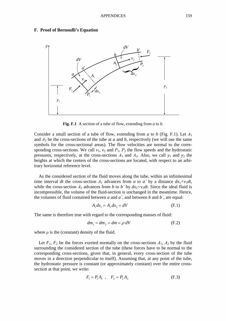
APPENDICES 159
F. Proof of Bernoulli’s Equation
y
1y
2y1F
2F
1P
2P
{
{
1dx
2dx1A
2A
1v
2vdV
dV
aa′
bb′
Fig. F.1 A section of a tube of flow, extending from a to b. Consider a small section of a tube of flow, extending from a to b (Fig. F.1). Let Α1 and Α2 be the cross-sections of the tube at a and b, respectively (we will use the same symbols for the cross-sectional areas). The flow velocities are normal to the corre-sponding cross-sections. We call v1, v2 and Ρ1, Ρ2 the flow speeds and the hydrostatic pressures, respectively, at the cross-sections Α1 and Α2. Also, we call y1 and y2 the heights at which the centers of the cross-sections are located, with respect to an arbi-trary horizontal reference level. As the considered section of the fluid moves along the tube, within an infinitesimal time interval dt the cross-section Α1 advances from a to a by a distance dx1=v1dt, while the cross-section Α2 advances from b to b by dx2=v2dt. Since the ideal fluid is incompressible, the volume of the fluid-section is unchanged in the meantime. Hence, the volumes of fluid contained between a and a , and between b and b , are equal:
1 1 2 2A dx A dx dV= = (F.1)
The same is therefore true with regard to the corresponding masses of fluid:
1 2dm dm dm dVρ= = = (F.2)
where ρ is the (constant) density of the fluid. Let F1, F2 be the forces exerted normally on the cross-sections Α1, Α2 by the fluid surrounding the considered section of the tube (these forces have to be normal to the corresponding cross-sections, given that, in general, every cross-section of the tube moves in a direction perpendicular to itself). Assuming that, at any point of the tube, the hydrostatic pressure is constant (or approximately constant) over the entire cross-section at that point, we write:
1 1 1 2 2 2,F P A F P A= = (F.3)
160 APPENDICES
We notice that F1 is in the direction of the flow, while F2 is opposite to the flow. This means that F1 produces work (its work is positive) while F2 consumes work (its work is negative). The total work of F1 and F2 for an elementary displacement of the sec-tion ab of the tube within time dt, is 1 1 2 2 1 1 1 2 2 2W F dx F dx P A dx P A dx= − = − ⇒
1 2( )W P P dV= − (F.4)
where we have used (F.3) and (F.1). From the discussion in Sec. 6.5, extended here to the case of a continuous medium, it follows that the work W of the forces F1 and F2 on the fluid-section ab, within a time dt, equals the change of the total mechanical energy of this section: ( )k p k pW E E E E= ∆ + = ∆ + ∆ (F.5)
We have:
( ) ( ) ( ) ( )k k a b k ab k bb k aaE E E E E′ ′ ′ ′∆ = − = − (F.6)
[Since the flow is steady, the quantity ( )k a bE ′ , for fixed a΄ and b, is constant in time;
thus it is eliminated by subtracting.] Now, by using (F.2), equation (F.6) is written:
2 2 2 22 1 2 1
1 1 1( ) ( ) ( )
2 2 2kE dm v dm v v v dm∆ = − = − ⇒
2 22 1
1( )
2kE v v dVρ∆ = − (F.7)
By similar reasoning, 2 1 2 1( ) ( ) ( ) ( ) ( ) ( )p p bb p aaE E E dm g y dm g y dm g y y′ ′∆ = − = − = − ⇒
2 1( )pE g y y dVρ∆ = − (F.8)
Substituting (F.4), (F.7) and (F.8) into (F.5), and eliminating dV, we find:
2 21 2 2 1 2 1
1( ) ( )
2P P v v g y yρ ρ− = − + − ⇒
2 21 1 1 2 2 2
1 1
2 2P v g y P v g yρ ρ ρ ρ+ + = + +
This is Bernoulli’s equation for an ideal flow. We note that both the equation of continuity (in the form we wrote it) and Ber-noulli’s equation can approximately be used for a gas (e.g., atmospheric air) in some limited region of space where the gas density does not vary appreciably from one point to another (the gas may thus be treated as an almost incompressible fluid in that region).
161
SOLVED PROBLEMS
PROBLEMS FOR CHAP. 2 – 3 1. The position of a particle moving along the x-axis is given as a function of time by the equation x=2t 3−3t 2+6t−5 , where x is in meters and t is in seconds. Find (a) the direction of motion at all times and (b) the time intervals during which the motion is accelerated or retarded. Does the particle ever stop? Solution: The algebraic values of velocity and acceleration are
26( 1) , 6(2 1) .dx dv
v t t a tdt dt
= = − + = = −
Hence, 236( 1)(2 1) .va t t t= − + − We notice that t2 – t+1>0 , for all values of t. Thus v>0 for all t, which means that the particle always moves in the positive direction of the x-axis, never stopping (even momentarily). Also, it is easy to verify that va>0 when t>0.5, while va<0 when t<0.5. Hence (cf. Sec. 2.4) the motion is retarded for t<0.5s and accelerated for t>0.5s. 2. A particle moves on the x-axis, having started at time t=0 from the point x=0 with initial velocity v=v0 . Find the velocity v and the position x of the particle as functions of time, as well as the velocity as a function of position x, if the acceleration of the particle is given as a function of velocity by (a) a= − kv ; (b) a= − kv 2 (where k is a positive constant). Solution: (a) Let a= − kv :
0 0
0
00
ln
(1)
v t
v
k t k t
dv dv dv vkv kdt k dt kt
dt v v v
ve v v e
v− −
= − ⇒ = − ⇒ = − ⇒ = − ⇒
= ⇒ =
∫ ∫
00 0 00 0
(1 ) (2)x tk t k t k t k tdx v
v e dx v e dt dx v e dt x edt k
− − − −= ⇒ = ⇒ = ⇒ = −∫ ∫
Eliminating e –kt from (1) and (2), we find: 0 (3)v v k x= −
Alternatively, dv = adt , dx = vdt , and, by dividing these,
0
00(3)
v x
v
dv ak dv kdx dv k dx v v k x
dx v= = − ⇒ = − ⇒ = − ⇒ − = − ⇒∫ ∫
(b) Let a= − kv 2 . Working similarly, show that
162 PROBLEMS
00 0
0
1, ln(1 ) , .
1k xv
v x kv t v v ekv t k
−= = + =+
3. A body moves on the x-axis with acceleration a=(4x–2)m/s 2, where x is the instan-taneous position of the body. The initial velocity of the body is v0=10m/s, at the initial location x0=0. Find the velocity v of the body as a function of position x. Solution: Since the acceleration a is given as a function of x, we use equation (2.5):
0
2 2 2 2 20 0
2 10 2 (4 2) 4( 25) .x x
xv v adx x dx v x x= + = + − ⇒ = − +∫ ∫
We notice that x2 – x+25>0 , for all values of x. Hence, 2 1/ 22( 25)v x x= ± − + . We
drop the negative sign, since it would yield v0= −10 for x=0, contrary to the given ini-tial condition. Thus, finally,
v = 2 (x2 – x+ 25)1/2 m/s . 4. A particle moves on the circumference of a circle. Its position at time t is given by the equation s=t 3+2t 2, where s is measured in meters along the circumference and where t is in seconds. The magnitude of the acceleration of the particle at time t=2s is
a=16 2 m/s 2. Find the radius R of the circle.
Solution: The magnitude of the velocity of the particle is 23 4ds
v t tdt
= = + .
We know that 22 2
2 2 2T N
dv va a a
dt R
= + = +
.
Hence, 2 4
2 22
(3 4 )(6 4)
t ta t
R
+= + + .
Setting t=2 and a=16 2 , and solving for R, we find: R=25m . 5. A particle moves on the xy-plane. Its coordinates x and y are given as functions of time t by the equations: x= t
2, y= (t−1)2, where t ≥ 1. Find: (a) The equation of the trajectory in the form F(x,y)= constant; (b) the components aT and aN of the acceleration, for all t; (c) the radius of curvature ρ, for all t. Solution: (a) Noting that x≥ 0, y≥ 0, and taking into account that t ≥ 1, we write:
x t= , 1y t= − . Eliminating t, we find: ( , ) 1F x y x y≡ − = .
(b) We have:
2 , 2( 1) , 2 , 2 .yxx y x y
dvdx dy dvv t v t a a
dt dt dt dt= = = = − = = = =

PROBLEMS 163
If |v�
| = v and |a�
| = a , a2 = ax
2 + ay2 = 8 , v2 = vx
2 + vy2 = 8t2 – 8t + 4 .
Hence, v = 2(2t2 – 2t + 1)1/2 . Note that v > 0 for all t.
Then, 2 1/ 2
4 2
(2 2 1)T
dv ta
dt t t
−= =
− + .
For aN we cannot make direct use of the relation aN = v2/ρ , since we do not yet know ρ. We thus proceed as follows:
2 2 2 2 22 2 1/ 2
4 28 8 .
2 2 1 (2 2 1)T N N T Na a a a a at t t t
+ = = ⇒ = − = ⇒ =− + − +
(c) 2 2
2 3/ 22(2 2 1) .NN
v va t t
aρ
ρ= ⇒ = = − +
6. Study the motion of a projectile (see figure). Find: (a) The time tA for the projectile to reach the highest point Α of the trajectory; (b) the maximum height h; (c) the time tB at which the projectile hits the ground at point Β; (d) the total horizontal distance R=OB; show that, for a given initial speed v0 , R is a maximum when the angle α is equal to 45 ο . (e) Show that the speed at Β is the same as the initial speed at Ο; also show that the angles α and β are equal. ( f ) Find the equation of the trajectory, in the form y=f(x).
i i x
y
O
R
A
B
h
α
βˆxu
ˆ yu
0v�
Av�
Bv�
g�
Fig. Problem 6 Solution: We assume that the projectile is ejected from Ο at time t=0, with initial ve-locity 0v
�
. The projectile moves with constant acceleration ˆya g gu= = −� �
; thus, its mo-
tion takes place in a constant vertical plane defined by the vectors of the initial veloc-
164 PROBLEMS
ity and the acceleration (cf. Sec. 2.5). Consider an arbitrary point of the trajectory, with position vector r
�
, and let v�
be the velocity of the projectile at that point. The vectors r
�
and v�
are given as functions of time by the equations (Sec. 2.5)
20 0
1,
2v v at r v t at= + = +� � � � � �
or, in component form,
0 0
20 0
ˆ ˆ ˆ ˆ ˆ( ) ,
1ˆ ˆ ˆ ˆ ˆ( ) .
2
x x y y x x y y y
x y x x y y y
v u v u v u v u gt u
xu yu v u v u t gt u
+ = + −
+ = + −
By equating the coefficients of ˆxu and ˆyu on the two sides of each equation, we ob-
tain the equations of motion of the projectile in the xy-plane:
0 0
20 0
. ,
1,
2
x x y y
x y
v v const v v gt
x v t y v t gt
= = = −
= = −
where 0 0 0 0 0 0cos , sin ( | |) .x yv v v v v vα α= = =
�
(Note that the motion is uniform in the horizontal direction and uniformly accelerated in the vertical direction.)
(a) At the highest point Α, 0 00
sin0 0 .y
y y A A
v vv v gt t
g g
α= ⇒ − = ⇒ = =
(b) 2 2 2
02 00
1 sin.
2 2 2y
A y A A
v vh y v t gt h
g g
α= = − ⇒ = =
(c) 020
210 0 2 .
2y
B y B B B A
vy v t gt t t
g= ⇒ − = ⇒ = =
(d ) 2 2
0 0 0 00
2 2 sin cos sin 2.x y
B x B
v v v vR x v t R
g g g
α α α= = = = ⇒ =
We notice that R=max when sin 2α=1 or α= 45ο . (e) At the return point Β, 0 0 0 0 0, 2 .x x y y B y y yv v v v gt v v v= = − = − = −
Thus, 2 2 2 2 2 20 0 0 0 0| | | | | | .B x y x y Bv v v v v v v v v= + = + = ⇒ = =
� � �
Moreover, 0
0
| |tan tan .
| |y y
x x
v v
v vβ α β α= = = ⇒ =
( f ) 00 0
.cosx
x
x xx v t t
v v α= ⇒ = = Then,
2 20 2 2
0
1(tan )
2 2 cosy
gy v t gt y x x
vα
α= − ⇒ = − +
which is an equation of the form y = κ x2 + λ x (equation of a parabola).
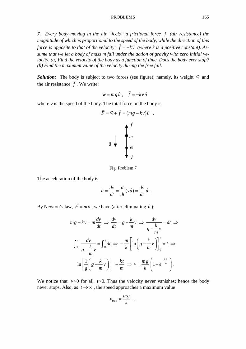
PROBLEMS 165
7. Every body moving in the air “feels” a frictional force f�
(air resistance) the magnitude of which is proportional to the speed of the body, while the direction of this
force is opposite to that of the velocity: f kv= −�
�
(where k is a positive constant). As-sume that we let a body of mass m fall under the action of gravity with zero initial ve-locity. (a) Find the velocity of the body as a function of time. Does the body ever stop? (b) Find the maximum value of the velocity during the free fall. Solution: The body is subject to two forces (see figure); namely, its weight w
�
and
the air resistance f�
. We write:
ˆ ˆ,w mg u f kvu= = −�
�
where v is the speed of the body. The total force on the body is
ˆ( )F w f mg kv u= + = −�� �
.
Fig. Problem 7
The acceleration of the body is
ˆ ˆ( )dv d dv
a vu udt dt dt
= = =�
�
.
By Newton’s law, F ma=
� �
, we have (after eliminating u ):
0 0
0
ln
1ln 1 .
vv t
k t
m
dv dv k dvmg kv m g v dt
kdt dt m g vm
dv m kdt g v t
k k mg vm
k kt mgg v v e
g m m k
−
− = ⇒ = − ⇒ = ⇒−
= ⇒ − − = ⇒ −
− = − ⇒ = −
∫ ∫
We notice that v>0 for all t>0. Thus the velocity never vanishes; hence the body never stops. Also, as t → ∞ , the speed approaches a maximum value
max
mgv
k= .
m
w�
f�
v�
u
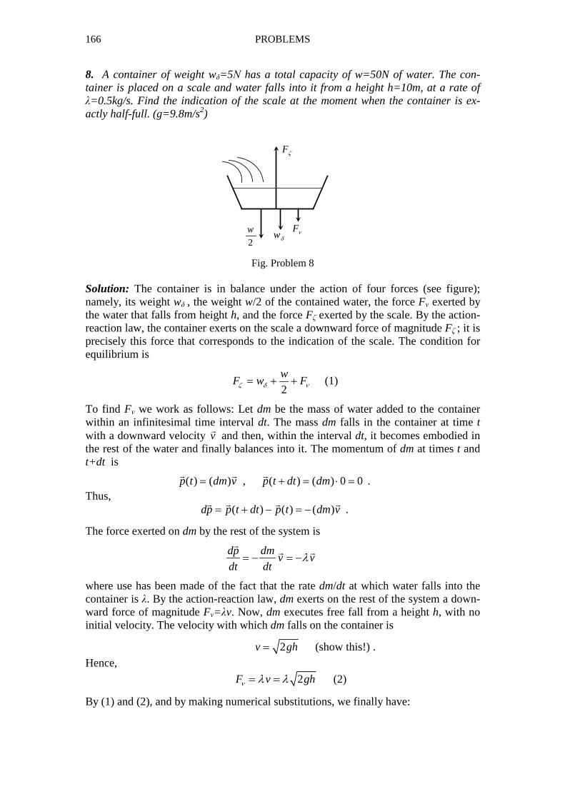
166 PROBLEMS
8. A container of weight wδ=5Ν has a total capacity of w=50N of water. The con-tainer is placed on a scale and water falls into it from a height h=10m, at a rate of λ=0.5kg/s. Find the indication of the scale at the moment when the container is ex-actly half-full. (g=9.8m/s2)
2
wwδ
Fν
Fζ
Fig. Problem 8 Solution: The container is in balance under the action of four forces (see figure); namely, its weight wδ , the weight w/2 of the contained water, the force Fν exerted by the water that falls from height h, and the force Fζ exerted by the scale. By the action-reaction law, the container exerts on the scale a downward force of magnitude Fζ ; it is precisely this force that corresponds to the indication of the scale. The condition for equilibrium is
2
wF w Fζ δ ν= + + (1)
To find Fν we work as follows: Let dm be the mass of water added to the container within an infinitesimal time interval dt. The mass dm falls in the container at time t with a downward velocity v
�
and then, within the interval dt, it becomes embodied in the rest of the water and finally balances into it. The momentum of dm at times t and t+dt is
( ) ( ) , ( ) ( ) 0 0p t dm v p t dt dm= + = ⋅ =� � �
. Thus, ( ) ( ) ( )dp p t dt p t dm v= + − = −
� � � �
.
The force exerted on dm by the rest of the system is
dp dm
v vdt dt
λ= − = −�
� �
where use has been made of the fact that the rate dm/dt at which water falls into the container is λ. By the action-reaction law, dm exerts on the rest of the system a down-ward force of magnitude Fν=λv. Now, dm executes free fall from a height h, with no initial velocity. The velocity with which dm falls on the container is
2v gh= (show this!) .
Hence,
2F v ghν λ λ= = (2)
By (1) and (2), and by making numerical substitutions, we finally have:
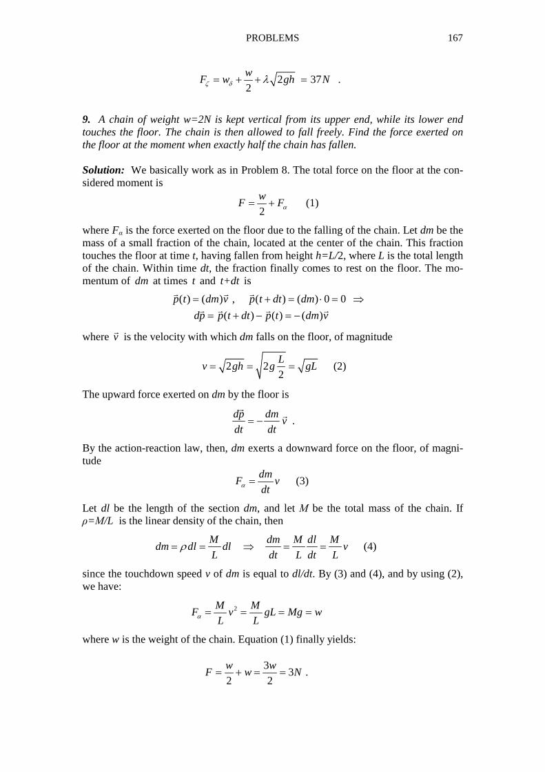
PROBLEMS 167
2 372
wF w gh Nζ δ λ= + + = .
9. A chain of weight w=2N is kept vertical from its upper end, while its lower end touches the floor. The chain is then allowed to fall freely. Find the force exerted on the floor at the moment when exactly half the chain has fallen. Solution: We basically work as in Problem 8. The total force on the floor at the con-sidered moment is
2
wF Fα= + (1)
where Fα is the force exerted on the floor due to the falling of the chain. Let dm be the mass of a small fraction of the chain, located at the center of the chain. This fraction touches the floor at time t, having fallen from height h=L/2, where L is the total length of the chain. Within time dt, the fraction finally comes to rest on the floor. The mo-mentum of dm at times t and t+dt is
( ) ( ) , ( ) ( ) 0 0
( ) ( ) ( )
p t dm v p t dt dm
dp p t dt p t dm v
= + = ⋅ = ⇒
= + − = −
� � �
� � � �
where v�
is the velocity with which dm falls on the floor, of magnitude
2 22
Lv gh g gL= = = (2)
The upward force exerted on dm by the floor is
dp dm
vdt dt
= −�
�
.
By the action-reaction law, then, dm exerts a downward force on the floor, of magni-tude
dm
F vdtα = (3)
Let dl be the length of the section dm, and let Μ be the total mass of the chain. If ρ=Μ/L is the linear density of the chain, then
M dm M dl M
dm dl dl vL dt L dt L
ρ= = ⇒ = = (4)
since the touchdown speed v of dm is equal to dl/dt. By (3) and (4), and by using (2), we have:
2M MF v gL Mg w
L Lα = = = =
where w is the weight of the chain. Equation (1) finally yields:
3
3 .2 2
w wF w N= + = =
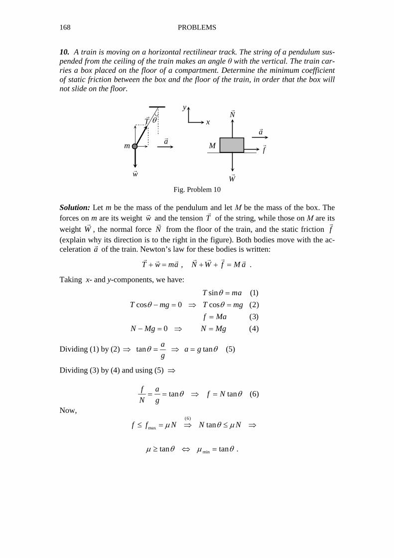
168 PROBLEMS
10. A train is moving on a horizontal rectilinear track. The string of a pendulum sus-pended from the ceiling of the train makes an angle θ with the vertical. The train car-ries a box placed on the floor of a compartment. Determine the minimum coefficient of static friction between the box and the floor of the train, in order that the box will not slide on the floor.
m
w�
T�
θ x
y
a�
a�
W�
M
N�
f�
Fig. Problem 10
Solution: Let m be the mass of the pendulum and let Μ be the mass of the box. The forces on m are its weight w
�
and the tension T�
of the string, while those on Μ are its
weight W�
, the normal force N�
from the floor of the train, and the static friction f�
(explain why its direction is to the right in the figure). Both bodies move with the ac-celeration a
�
of the train. Newton’s law for these bodies is written:
,T w ma N W f M a+ = + + =�� � �� � �
.
Taking x- and y-components, we have:
sin (1)
cos 0 cos (2)
(3)
0 (4)
T ma
T mg T mg
f Ma
N Mg N Mg
θθ θ
=
− = ⇒ =
=
− = ⇒ =
Dividing (1) by (2) tan tana
a gg
θ θ⇒ = ⇒ = (5)
Dividing (3) by (4) and using (5) ⇒
tan tanf a
f NN g
θ θ= = ⇒ = (6)
Now,
(6)
max
min
tan
tan tan .
f f N N Nµ θ µ
µ θ µ θ
≤ = ⇒ ≤ ⇒
≥ ⇔ =
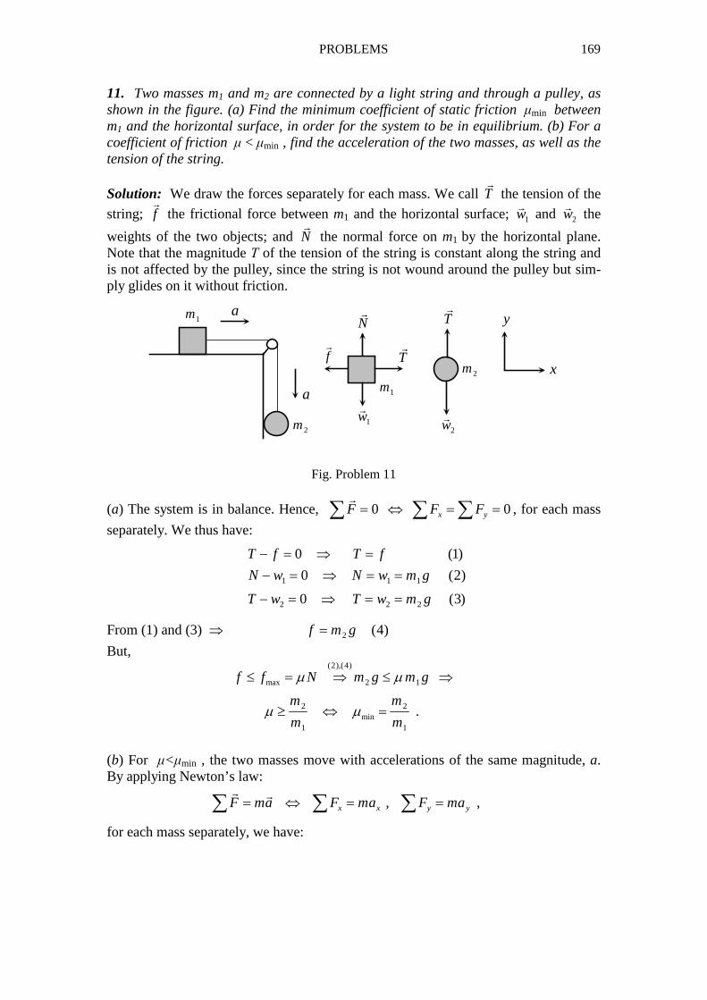
PROBLEMS 169
11. Two masses m1 and m2 are connected by a light string and through a pulley, as shown in the figure. (a) Find the minimum coefficient of static friction µmin between m1 and the horizontal surface, in order for the system to be in equilibrium. (b) For a coefficient of friction µ < µmin , find the acceleration of the two masses, as well as the tension of the string. Solution: We draw the forces separately for each mass. We call T
�
the tension of the
string; f�
the frictional force between m1 and the horizontal surface; 1w�
and 2w�
the
weights of the two objects; and N�
the normal force on m1 by the horizontal plane. Note that the magnitude Τ of the tension of the string is constant along the string and is not affected by the pulley, since the string is not wound around the pulley but sim-ply glides on it without friction.
1m
1m
2m
2m
a
a
T�
T�
N�
f�
1w�
2w�
x
y
Fig. Problem 11
(a) The system is in balance. Hence, 0 0x yF F F= ⇔ = =∑ ∑ ∑
�
, for each mass
separately. We thus have:
1 1 1
2 2 2
0 (1)
0 (2)
0 (3)
T f T f
N w N w m g
T w T w m g
− = ⇒ =
− = ⇒ = =
− = ⇒ = =
From (1) and (3) ⇒ 2 (4)f m g=
But,
(2),(4)
max 2 1
2 2min
1 1
.
f f N m g m g
m m
m m
µ µ
µ µ
≤ = ⇒ ≤ ⇒
≥ ⇔ =
(b) For µ<µmin , the two masses move with accelerations of the same magnitude, a. By applying Newton’s law:
,x x y yF ma F ma F ma= ⇔ = =∑ ∑ ∑� �
,
for each mass separately, we have:
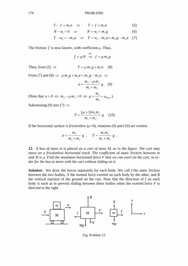
170 PROBLEMS
1 1
1 1 1
2 2 2 2 2 2
(5)
0 (6)
(7)
T f m a T f m a
N w N w m g
T w m a T w m a m g m a
− = ⇒ = +
− = ⇒ = =
− = − ⇒ = − = −
The friction f is now kinetic, with coefficient µ. Thus,
(6)
1 .f N f m gµ µ= ⇒ =
Then, from (5) ⇒ 1 1T m g m aµ= + (8)
From (7) and (8) 1 1 2 2m g m a m g m aµ⇒ + = − ⇒
2 1
1 2
m ma g
m m
µ−=
+ (9)
(Note that 22 1 min
1
0 0m
a m mm
µ µ µ> ⇔ − > ⇔ < = .)
Substituting (9) into (7) ⇒
1 2
1 2
( 1)m mT g
m m
µ +=
+ (10)
If the horizontal surface is frictionless (µ=0), relations (9) and (10) are written:
2 1 2
1 2 1 2
,m m m
a g T gm m m m
= =+ +
.
12. A box of mass m is placed on a cart of mass Μ, as in the figure. The cart may move on a frictionless horizontal track. The coefficient of static friction between m and Μ is µ. Find the maximum horizontal force F that we can exert on the cart, in or-der for the box to move with the cart without sliding on it. Solution: We draw the forces separately for each body. We call f the static friction between the two bodies, Ν the normal force exerted on each body by the other, and R the vertical reaction of the ground on the cart. Note that the direction of f on each body is such as to prevent sliding between these bodies when the exerted force F is directed to the right.
m
mM M
a
F Ff
MgN
NR
f
mg
x
y
Fig. Problem 12

PROBLEMS 171
If no sliding occurs, the two bodies move with a common acceleration, a. We apply Newton’s law in the x- and y-directions, for each body separately:
(1)
0 (2)
(3)
0 (4)
F f Ma F Ma f
R Mg N R Mg N
f ma
N mg N mg
− = ⇒ = +
− − = ⇒ = +
=
− = ⇒ =
From (2) and (4) ⇒ R= (M+m) g . From (1) and (3) ⇒ F= (M+m) a (5) [equation (5) is simply Newton’s law for the system (M+m)]. Now,
(3),(4)
max (6)f f N ma mg a gµ µ µ≤ = ⇒ ≤ ⇒ ≤
Equation (6) gives the allowed values of the acceleration in order that the masses move together, with no sliding on each other. From (5) and (6) we find the allowed values of the external force F : max( ) ( ) .F M m g F M m gµ µ≤ + ⇔ = +
13. A cart, moving on a horizontal track, pushes a box, as shown in the figure. Find the values of the acceleration of the cart in order that the box will not fall to the ground. The coefficient of static friction between the box and the cart is µ. Solution: Let a be the common acceleration of the box and the cart. We call m the mass of the box, f the static friction between the box and the cart, and Ν the normal force on the box by the cart.
m
a
f
N
mgx
y
Fig. Problem 13
By Newton’s law for the box: ,x x y yF ma F ma F maΣ = ⇔ Σ = Σ =
� �
, we have:
(1)
0 (2)
N ma
f mg f mg
=
− = ⇒ =
But,
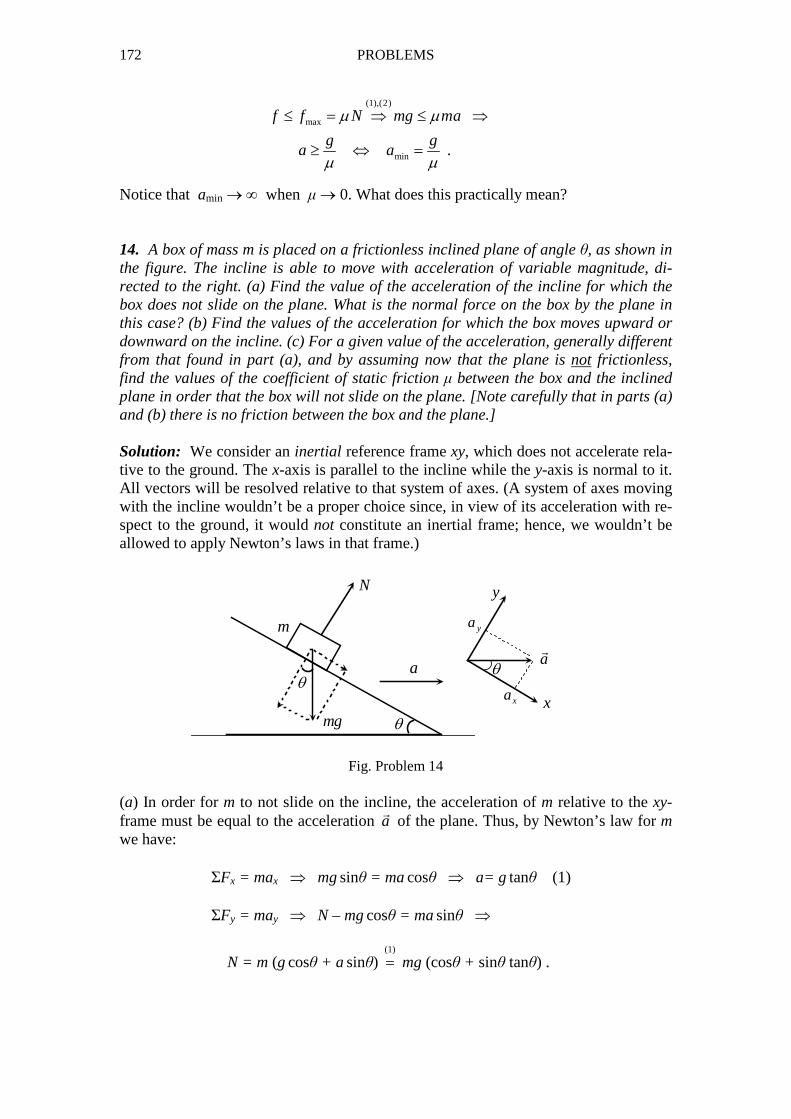
172 PROBLEMS
(1),(2)
max
min .
f f N mg ma
g ga a
µ µ
µ µ
≤ = ⇒ ≤ ⇒
≥ ⇔ =
Notice that amin → ∞ when µ → 0. What does this practically mean? 14. A box of mass m is placed on a frictionless inclined plane of angle θ, as shown in the figure. The incline is able to move with acceleration of variable magnitude, di-rected to the right. (a) Find the value of the acceleration of the incline for which the box does not slide on the plane. What is the normal force on the box by the plane in this case? (b) Find the values of the acceleration for which the box moves upward or downward on the incline. (c) For a given value of the acceleration, generally different from that found in part (a), and by assuming now that the plane is not frictionless, find the values of the coefficient of static friction µ between the box and the inclined plane in order that the box will not slide on the plane. [Note carefully that in parts (a) and (b) there is no friction between the box and the plane.] Solution: We consider an inertial reference frame xy, which does not accelerate rela-tive to the ground. The x-axis is parallel to the incline while the y-axis is normal to it. All vectors will be resolved relative to that system of axes. (A system of axes moving with the incline wouldn’t be a proper choice since, in view of its acceleration with re-spect to the ground, it would not constitute an inertial frame; hence, we wouldn’t be allowed to apply Newton’s laws in that frame.)
θ
θ
a a�
m
mg
N
x
y
θ
xa
ya
Fig. Problem 14 (a) In order for m to not slide on the incline, the acceleration of m relative to the xy-frame must be equal to the acceleration a
�
of the plane. Thus, by Newton’s law for m we have: ΣFx = max ⇒ mg sinθ = ma cosθ ⇒ a= g tanθ (1) ΣFy = may ⇒ N – mg cosθ = ma sinθ ⇒
N = m (g cosθ + a sinθ) (1)
= mg (cosθ + sinθ tanθ) .
PROBLEMS 173
(b) In order for m to slide on the incline, its acceleration a′�
must differ from the ac-celeration a
�
of the plane. Here we only need to consider the x-component of the ac-celeration (the one parallel to the plane): ΣFx = max΄ ⇒ mg sinθ = max΄ ⇒ ax΄= g sinθ . The body will slide downward if ax΄ > ax or g sinθ > a cosθ ⇒ a < g tanθ (downward) (2) while it will slide upward if ax΄ < ax or g sinθ < a cosθ ⇒ a > g tanθ (upward) (3) (c) Conditions (2) and (3) describe the tendency of m to move downward or upward, respectively, relative to the incline when no static friction is present. Hence, friction is necessary in order that m doesn’t slide on the plane, for accelerations a of the incline that are different from that given by relation (1). Obviously, the friction f will be di-rected upward or downward along the plane, depending on whether the acceleration of the latter obeys (2) or (3), respectively. Taking cases (2) and (3) separately, as well as taking into account that
f < fmax = µΝ , show that
| sin cos |
.cos sin
g a
g a
θ θµ
θ θ−
≥+
15. A satellite moves in a circular orbit about the Earth. Inside the satellite an ob-server is studying the motion of an object of mass m. (a) Explain why a use of New-ton’s laws would lead this observer to physically incorrect conclusions. (b) As an ex-ample, show that, according to this observer, the object m is weightless! Solution: The satellite is in free fall since it moves under the sole action of gravity, with acceleration equal to the acceleration of gravity, g
�
. (Don’t be deceived by the fact that it moves circularly rather than falling straight down to the Earth! The vector g�
is always directed toward the Earth and plays here the role of centripetal accelera-tion. The satellite would fall straight down hadn’t it been given an initial velocity per-pendicular to the local direction of the radius of the Earth.) The accelerating satellite is an example of a non-inertial frame of reference. An observer moving with the satel-lite (non-inertial observer) will come to incorrect conclusions if she tries to interpret her measurements physically by using Newton’s laws. To understand this, we need to say a few things regarding measurements in non-inertial frames, in general. We consider two observers: an inertial one, Ο, at rest on the surface of the Earth, and a non-inertial one, Ο΄, moving with an acceleration A
�
relative to O. Both observers study the motion of a particle of mass m and record respective accelerations a
�
and a′�
. By recalling what was said in Sec. 2.8 regarding relative acceleration, it is not hard to see that

174 PROBLEMS
a a A′ = −�� �
(1)
Since Ο is an inertial observer, he may use Newton’s law to relate the measured ac-celeration a
�
with the total force F�
acting on the particle, which force is due to all interactions in which this particle participates. We thus have:
(1)
( ) (2)F ma F m a A ma F mA F′ ′ ′= ⇒ = + ⇒ = − ≡� �� � � �� � �
The vector a′
�
on the left-hand side of (2) is the acceleration of m as measured by ob-server Ο΄. We notice that, if observer Ο΄ chooses to use Newton’s law in her non-inertial frame of reference, she will come to the conclusion that, in addition to the ac-tual force F
�
(which has the same value for all inertial observers; cf. Sec. 3.2) the par-
ticle is subject to another, fictitious force (“pseudo-force”) equal to mA−�
, which, of course, does not result from any real interactions but is simply an effect related to the acceleration of Ο΄. Thus, if observer Ο΄ insists on using Newton’s law after measuring the acceleration a′
�
, she will make a wrong evaluation, F ′�
, of the total force on m, different from the real force F
�
evaluated by the inertial observer Ο.
Fig. Problem 15 As an example, assume that the observer Ο΄ is in a chamber moving with acceleration A�
relative to the Earth (thus, relative to the inertial observer Ο who is at rest on the surface of the Earth). Observer O΄ wants to determine the weight of an object of mass m by using a scale hanging from the ceiling of the chamber, as shown in the figure. The true total force on the body is F mg T= +
� ��
, where T�
is the tension of the string
from which the body is suspended. The magnitude Τ of T�
corresponds to the indica-tion of the scale. The acceleration of m with respect to the inertial observer Ο is A
�
. Thus, Newton’s law for this observer is written:
F mg T mA= + =�� ��
(3)
O′
A�
m
T�
mg�
O
Earth
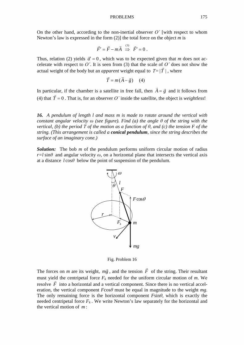
PROBLEMS 175
On the other hand, according to the non-inertial observer Ο΄ [with respect to whom Newton’s law is expressed in the form (2)] the total force on the object m is
(3)
0 .F F mA F′ ′= − ⇒ =�� � �
Thus, relation (2) yields 0a′ =�
, which was to be expected given that m does not ac-celerate with respect to Ο΄. It is seen from (3) that the scale of Ο΄ does not show the actual weight of the body but an apparent weight equal to Τ= |T
�
| , where
( )T m A g= −�� �
(4)
In particular, if the chamber is a satellite in free fall, then A g=� �
and it follows from
(4) that 0T =�
. That is, for an observer Ο΄ inside the satellite, the object is weightless! 16. A pendulum of length l and mass m is made to rotate around the vertical with constant angular velocity ω (see figure). Find (a) the angle θ of the string with the vertical, (b) the period Τ of the motion as a function of θ, and (c) the tension F of the string. (This arrangement is called a conical pendulum, since the string describes the surface of an imaginary cone.) Solution: The bob m of the pendulum performs uniform circular motion of radius r=l sinθ and angular velocity ω, on a horizontal plane that intersects the vertical axis at a distance l cosθ below the point of suspension of the pendulum.
⋅
•r
ω
lθF
m
mg
v
kF
cosF θ
Fig. Problem 16 The forces on m are its weight, mg
�
, and the tension F�
of the string. Their resultant must yield the centripetal force Fk needed for the uniform circular motion of m. We resolve F
�
into a horizontal and a vertical component. Since there is no vertical accel-eration, the vertical component Fcosθ must be equal in magnitude to the weight mg. The only remaining force is the horizontal component Fsinθ, which is exactly the needed centripetal force Fk . We write Newton’s law separately for the horizontal and the vertical motion of m :
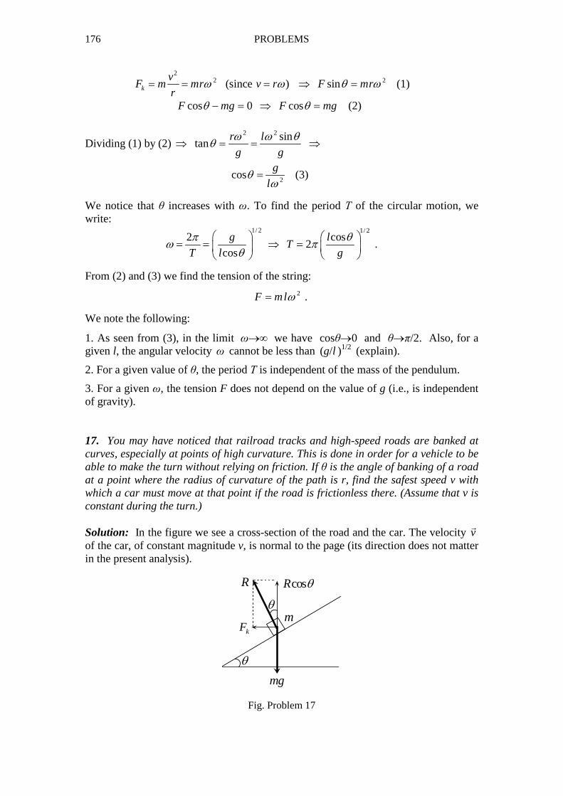
176 PROBLEMS
2
2 (since )k
vF m mr v r
rω ω= = = 2sinF mrθ ω⇒ = (1)
cos 0 cosF mg F mgθ θ− = ⇒ = (2)
Dividing (1) by (2) 2 2 sin
tanr l
g g
ω ω θθ⇒ = = ⇒
2
cosg
lθ
ω= (3)
We notice that θ increases with ω. To find the period Τ of the circular motion, we write:
1/ 2 1/ 2
2 cos2
cos
g lT
T l g
π θω π
θ
= = ⇒ =
.
From (2) and (3) we find the tension of the string:
2F mlω= .
We note the following:
1. As seen from (3), in the limit ω→∞ we have cosθ→0 and θ→π/2. Also, for a given l, the angular velocity ω cannot be less than (g/l )
1/2 (explain).
2. For a given value of θ, the period Τ is independent of the mass of the pendulum.
3. For a given ω, the tension F does not depend on the value of g (i.e., is independent of gravity). 17. You may have noticed that railroad tracks and high-speed roads are banked at curves, especially at points of high curvature. This is done in order for a vehicle to be able to make the turn without relying on friction. If θ is the angle of banking of a road at a point where the radius of curvature of the path is r, find the safest speed v with which a car must move at that point if the road is frictionless there. (Assume that v is constant during the turn.) Solution: In the figure we see a cross-section of the road and the car. The velocity v
�
of the car, of constant magnitude v, is normal to the page (its direction does not matter in the present analysis).
θ
θm
mg
R
kF
cosR θ
Fig. Problem 17
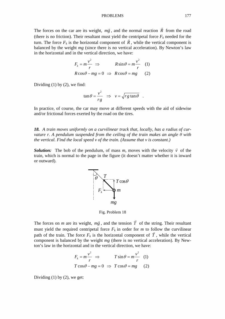
PROBLEMS 177
The forces on the car are its weight, mg�
, and the normal reaction R�
from the road (there is no friction). Their resultant must yield the centripetal force Fk needed for the turn. The force Fk is the horizontal component of R
�
, while the vertical component is balanced by the weight mg (since there is no vertical acceleration). By Newton’s law in the horizontal and in the vertical direction, we have:
2 2
sin (1)
cos 0 cos (2)
k
v vF m R m
r rR mg R mg
θ
θ θ
= ⇒ =
− = ⇒ =
Dividing (1) by (2), we find:
2
tan tanv
v rgrg
θ θ= ⇒ = .
In practice, of course, the car may move at different speeds with the aid of sidewise and/or frictional forces exerted by the road on the tires. 18. A train moves uniformly on a curvilinear track that, locally, has a radius of cur-vature r. A pendulum suspended from the ceiling of the train makes an angle θ with the vertical. Find the local speed v of the train. (Assume that v is constant.) Solution: The bob of the pendulum, of mass m, moves with the velocity v
�
of the train, which is normal to the page in the figure (it doesn’t matter whether it is inward or outward).
m
mg
T
kF
cosT θθ
Fig. Problem 18 The forces on m are its weight, mg
�
, and the tension T�
of the string. Their resultant must yield the required centripetal force Fk in order for m to follow the curvilinear path of the train. The force Fk is the horizontal component of T
�
, while the vertical component is balanced by the weight mg (there is no vertical acceleration). By New-ton’s law in the horizontal and in the vertical direction, we have:
2 2
sin (1)
cos 0 cos (2)
k
v vF m T m
r rT mg T mg
θ
θ θ
= ⇒ =
− = ⇒ =
Dividing (1) by (2), we get:
178 PROBLEMS
2
tan tanv
v rgrg
θ θ= ⇒ = .
19. According to Newton’s Law of Gravity, two masses m1 and m2 , a distance r apart, attract each other with a force
1 22
m mF G
r=
where G is a constant. (For a rigid body, the distance r is measured from the center of mass of the body.) We call Μ the mass and R the radius of the Earth. (a) Find an ex-pression for the acceleration g of gravity near the surface of the Earth. (b) A satellite moves in a circular orbit about the Earth, with constant speed and at a height h above the surface of the Earth. Find the speed v of the satellite, as well as the period Τ of the circular motion. Solution: (a) Consider a body of mass m located near the surface of the Earth, thus at a distance r=R from its center. The Earth attracts the body with a force equal to the weight of the body:
2
mMF G
R= (1)
Now, if g is the acceleration of gravity near the surface of the Earth, and if the body is only subject to the gravitational interaction, then, by Newton’s second law,
F mg= (2)
By comparing (1) and (2), we have:
2
Mg G
R= .
Note that g does not depend on m. This means that, near the surface of the Earth, all bodies move under the action of gravity with a common acceleration g (provided, of course, that they are not subject to any additional, non-gravitational interactions). (b) The radius of the circular path of the satellite is r=R+h. Since the speed v of the satellite is constant, the satellite is only subject to a centripetal force equal to the gravitational attraction from the Earth. Hence, if m is the mass of the satellite,
2
2
v mM GM GMm G v
r r r R h= ⇒ = =
+ (3)
Note again that the result is independent of m. We also have:
3/ 2(3)2 2 2 ( )r r R h
v r T TT v GM
π π πω
+= = ⇒ = ⇒ = .
PROBLEMS 179
20. A particle moves on the xy-plane under the action of a force F v A= �� �
, where v�
is the velocity of the particle and where A�
is a constant vector parallel to the z-axis. (a) Show that F
�
is a vector belonging to the xy-plane and determine the direction of F�
relative to the trajectory of the particle. (b) Show that v�
and F�
are vectors of constant magnitude. (c) Show that the particle executes uniform circular motion.
Solution: (a) Let ˆ ˆx x y yv v u v u= +�
and ˆzA Au=�
, where | |A A=�
(we chose A�
to be in
the positive direction of the z-axis). Then,
ˆ ˆ ˆ ˆ ˆ( ) ( ) ( )x x y y z y x x yF v A v u v u Au A v u v u= × = + × = −�� �
which is a vector in the xy-plane. Moreover, by the definition of the vector product, F�
is normal to the velocity v�
, hence normal to the trajectory. This can also be seen as follows:
ˆ ˆ ˆ ˆ( ) ( ) ( ) 0y x x y x x y y y x x yF v A v u v u v u v u A v v v v⋅ = − ⋅ + = − =� �
.
(b) Since the total force F�
is normal to the velocity, the speed | |v v=�
is constant (only the direction of motion changes). Furthermore,
| | | || | sin constant2
F F v A vAπ
≡ = = =�� �
.
(c) Let ρ be the radius of curvature at an arbitrary point of the trajectory, and let m be the mass of the particle. Since F
�
is centripetal at all points of the path,
2 2
constantv mv
F mF
ρρ
= ⇒ = =
(since both v and F are constant). We thus have a uniform motion on a plane, along a path with constant radius of curvature. What kind of motion is this? 21. A particle of mass m is moving on the xy-plane. Its coordinates are given as func-tions of time by the equations: x = A cos ωt , y = A sin ωt , where A , ω are positive constants. (a) Find the equation of the trajectory of the particle, in the form F(x,y)= const. (b) Find the velocity ( , )x yv v v≡
�
and the acceleration ( , )x ya a a≡�
of the particle as
functions of time and show that these vectors are mutually perpendicular at every point of the trajectory. What do you conclude about the speed of the particle? Verify your conclusion by calculating this speed directly. (c) Find the tangential and the normal acceleration as functions of time. (d) Find the radius of curvature, ρ, as a function of time and show that your result is consistent with that of part (a). Characterize the type of motion of the particle. (e) Show that the particle is subject to a total force of constant magnitude. How is this force oriented relative to the trajectory? (f ) Show that the angular momentum of the particle, with respect to the origin Ο of the coordinate system (x, y), is constant in time. What do you conclude regarding the total torque on the particle about O?
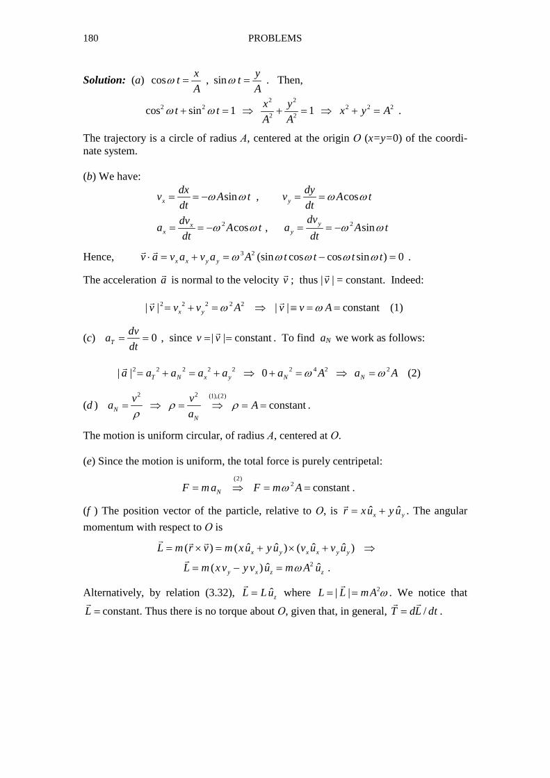
180 PROBLEMS
Solution: (a) cos , sinx y
t tA A
ω ω= = . Then,
2 2
2 2 2 2 22 2
cos sin 1 1x y
t t x y AA A
ω ω+ = ⇒ + = ⇒ + = .
The trajectory is a circle of radius Α, centered at the origin Ο (x=y=0) of the coordi-nate system. (b) We have:
2 2
sin , cos
cos , sin
x y
yxx y
dx dyv A t v A t
dt dtdvdv
a A t a A tdt dt
ω ω ω ω
ω ω ω ω
= = − = =
= = − = = −
Hence, 3 2 (sin cos cos sin ) 0x x y yv a v a v a A t t t tω ω ω ω ω⋅ = + = − =� �
.
The acceleration a�
is normal to the velocity v�
; thus |v�
| = constant. Indeed: 2 2 2 2 2| | | | constantx yv v v A v v Aω ω= + = ⇒ ≡ = =
� �
(1)
(c) 0T
dva
dt= = , since | |v v= =
�
constant . To find aN we work as follows:
2 2 2 2 2 2 4 2 2| | 0T N x y N Na a a a a a A a Aω ω= + = + ⇒ + = ⇒ =�
(2)
(d ) 2 2 (1),(2)
constantNN
v va A
aρ ρ
ρ= ⇒ = ⇒ = = .
The motion is uniform circular, of radius Α, centered at Ο. (e) Since the motion is uniform, the total force is purely centripetal:
(2)
2 constantNF m a F m Aω= ⇒ = = .
(f ) The position vector of the particle, relative to Ο, is ˆ ˆx yr xu y u= +�
. The angular
momentum with respect to Ο is
2
ˆ ˆ ˆ ˆ( ) ( ) ( )
ˆ ˆ( ) .
x y x x y y
y x z z
L m r v m xu yu v u v u
L m xv y v u m A uω
= × = + × + ⇒
= − =
� � �
�
Alternatively, by relation (3.32), ˆzL Lu=�
where 2| |L L mAω= =�
. We notice that
L =�
constant. Thus there is no torque about Ο, given that, in general, /T dL dt=� �
.
PROBLEMS 181
PROBLEMS FOR CHAP. 4 – 6 22. A particle of mass m is moving on a circle of radius R. We call L the magnitude of the angular momentum of the particle relative to the center Ο of the circle. (a) Show that the kinetic energy of the particle is
2 2
22 2k
L LE
mR I= =
where I=mR2 is the moment of inertia of m with respect to the axis of rotation (this axis is normal to the plane of the circle and passes through the center of the circle). (b) If the circular motion is uniform, show that the magnitude of the total force on the particle is
2
3
LF
mR= .
Solution: (a) We know that
2
21
2 2k
pE mv
m= = where p mv= .
Moreover, for circular motion [see equation (3.32)],
L
L mRv R p pR
= = ⇒ = .
Thus,
2 2 2
2
1
2 2 2k
L L LE
m R mR I = = =
.
(b) If the motion is uniform, the total force is purely centripetal:
22 2
3
v m L LF m
R R mR mR = = =
.
23. An electrically charged particle of charge q, moving with velocity v
�
inside a magnetic field of strength B
�
, is subject to a magnetic force ( )F q v B= � ��
. (a) Show
that F�
does not produce any work. (b) If no other forces act on the particle, what do you conclude regarding the particle’s kinetic energy? Solution: (a) The work of F
�
from a point a to a point b is
( ) 0b b b
a a a
drW F dr F dt F v dt
dt= ⋅ = ⋅ = ⋅ =∫ ∫ ∫
�� � �� �
since ( ) 0F v q v B v⋅ = × ⋅ =
� �� � �
(explain why!) .
(b) By the work-energy theorem, W=∆Ek = 0 ⇒ Ek = constant . Alternatively, since the total force F
�
is normal to the velocity v�
, the speed v is constant. Hence, Ek = mv2/2 = constant.
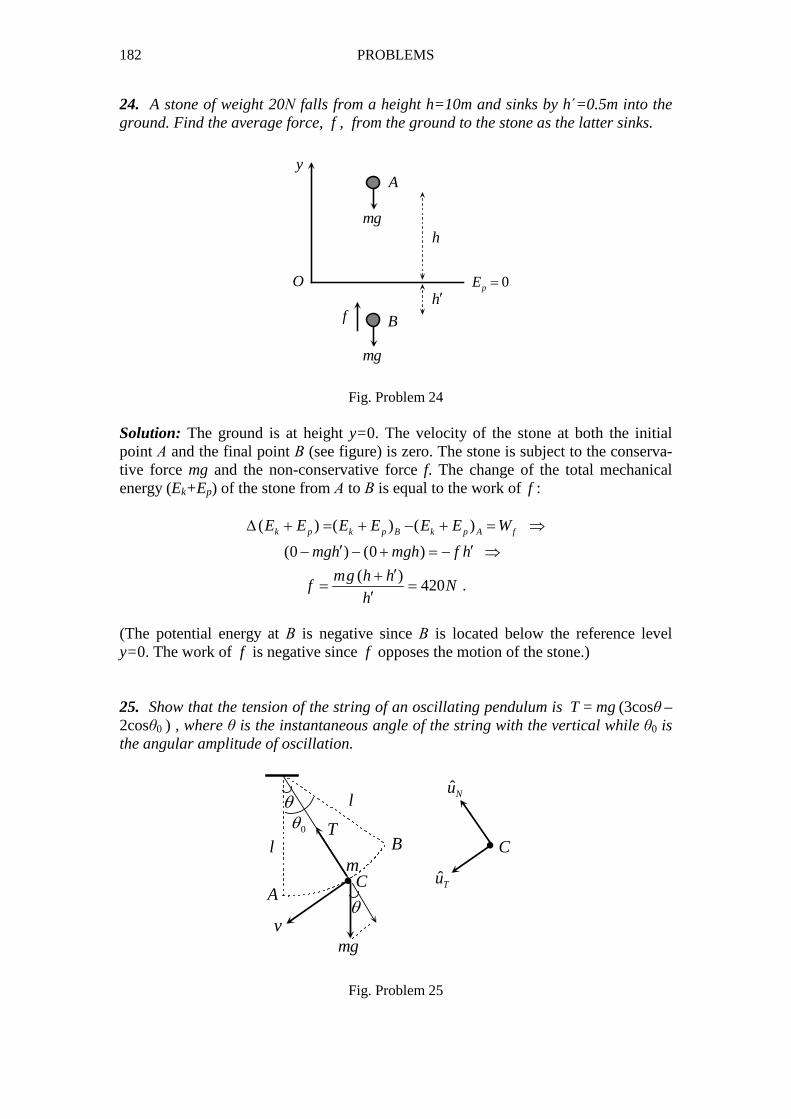
182 PROBLEMS
24. A stone of weight 20Ν falls from a height h=10m and sinks by h΄=0.5m into the ground. Find the average force, f , from the ground to the stone as the latter sinks.
Fig. Problem 24 Solution: The ground is at height y=0. The velocity of the stone at both the initial point Α and the final point Β (see figure) is zero. The stone is subject to the conserva-tive force mg and the non-conservative force f. The change of the total mechanical energy (Ek+Ep) of the stone from Α to Β is equal to the work of f :
( ) ( ) ( )
(0 ) (0 )
( )420 .
k p k p B k p A fE E E E E E W
mgh mgh f h
mg h hf N
h
∆ + = + − + = ⇒
′ ′− − + = − ⇒
′+= =
′
(The potential energy at Β is negative since Β is located below the reference level y=0. The work of f is negative since f opposes the motion of the stone.) 25. Show that the tension of the string of an oscillating pendulum is T = mg (3cosθ –
2cosθ0 ) , where θ is the instantaneous angle of the string with the vertical while θ0 is the angular amplitude of oscillation.
•
θ0θ
•
A
B
C
Cm
θ
l
l
T
vmg
ˆTu
ˆNu
Fig. Problem 25
O
y
0pE =
A
B
mg
mg
f
h
h′
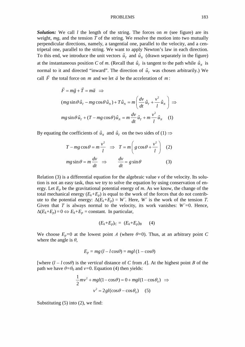
PROBLEMS 183
Solution: We call l the length of the string. The forces on m (see figure) are its weight, mg, and the tension Τ of the string. We resolve the motion into two mutually perpendicular directions, namely, a tangential one, parallel to the velocity, and a cen-tripetal one, parallel to the string. We want to apply Newton’s law in each direction. To this end, we introduce the unit vectors ˆTu and ˆNu (drawn separately in the figure)
at the instantaneous position C of m. (Recall that Tu is tangent to the path while ˆNu is
normal to it and directed “inward”. The direction of ˆTu was chosen arbitrarily.) We
call F�
the total force on m and we let a�
be the acceleration of m :
2
2
ˆ ˆ ˆ ˆ ˆ( sin cos )
ˆ ˆ ˆ ˆsin ( cos ) (1)
T N N T N
T N T N
F mg T ma
dv vmg u mg u T u m u u
dt l
dv vmg u T mg u m u m u
dt l
θ θ
θ θ
= + = ⇒
− + = + ⇒
+ − = +
� �� �
By equating the coefficients of ˆNu and ˆTu on the two sides of (1) ⇒
2 2
cos cos (2)
sin sin (3)
v vT mg m T m g
l l
dv dvmg m g
dt dt
θ θ
θ θ
− = ⇒ = +
= ⇒ =
Relation (3) is a differential equation for the algebraic value v of the velocity. Its solu-tion is not an easy task, thus we try to solve the equation by using conservation of en-ergy. Let Ep be the gravitational potential energy of m. As we know, the change of the total mechanical energy (Ek+Ep) is equal to the work of the forces that do not contrib-ute to the potential energy: ∆(Ek+Ep) = W΄. Here, W΄ is the work of the tension Τ. Given that Τ is always normal to the velocity, its work vanishes: W΄=0. Hence, ∆(Ek+Ep) = 0 ⇔ Ek+Ep = constant. In particular, (Ek+Ep)C = (Ek+Ep)B (4) We choose Ep=0 at the lowest point Α (where θ=0). Thus, at an arbitrary point C where the angle is θ, Ep = mg (l – l cosθ) = mgl (1 – cosθ) [where (l – l cosθ) is the vertical distance of C from Α]. At the highest point Β of the path we have θ=θ0 and v=0. Equation (4) then yields:
2
0
20
1(1 cos ) 0 (1 cos )
22 (cos cos ) (5)
mv mgl mgl
v gl
θ θ
θ θ
+ − = + − ⇒
= −
Substituting (5) into (2), we find:
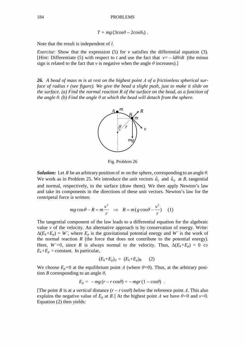
184 PROBLEMS
T = mg (3cosθ – 2cosθ0) . Note that the result is independent of l.
Exercise: Show that the expression (5) for v satisfies the differential equation (3). [Hint: Differentiate (5) with respect to t and use the fact that v= – ldθ/dt (the minus sign is related to the fact that v is negative when the angle θ increases).] 26. A bead of mass m is at rest on the highest point Α of a frictionless spherical sur-face of radius r (see figure). We give the bead a slight push, just to make it slide on the surface. (a) Find the normal reaction R of the surface on the bead, as a function of the angle θ. (b) Find the angle θ at which the bead will detach from the sphere.
••
i
θ
AB
m
m
mg
r v
R
Fig. Problem 26 Solution: Let Β be an arbitrary position of m on the sphere, corresponding to an angle θ. We work as in Problem 25. We introduce the unit vectors ˆTu and ˆNu at Β, tangential
and normal, respectively, to the surface (draw them). We then apply Newton’s law and take its components in the directions of these unit vectors. Newton’s law for the centripetal force is written:
2 2
cos ( cos )v v
mg R m R m gr r
θ θ− = ⇒ = − (1)
The tangential component of the law leads to a differential equation for the algebraic value v of the velocity. An alternative approach is by conservation of energy. Write: ∆(Ek+Ep) = W΄, where Ep is the gravitational potential energy and W΄ is the work of the normal reaction R (the force that does not contribute to the potential energy). Here, W΄=0, since R is always normal to the velocity. Thus, ∆(Ek+Ep) = 0 ⇔ Ek+Ep = constant. In particular,
(Ek+Ep)Α = (Ek+Ep)B (2)
We choose Ep=0 at the equilibrium point Α (where θ=0). Thus, at the arbitrary posi-tion Β corresponding to an angle θ,
Ep = − mg (r – r cosθ) = − mgr (1 – cosθ) .
[The point Β is at a vertical distance (r – r cosθ) below the reference point Α. This also explains the negative value of Ep at Β.] At the highest point Α we have θ=0 and v=0. Equation (2) then yields:
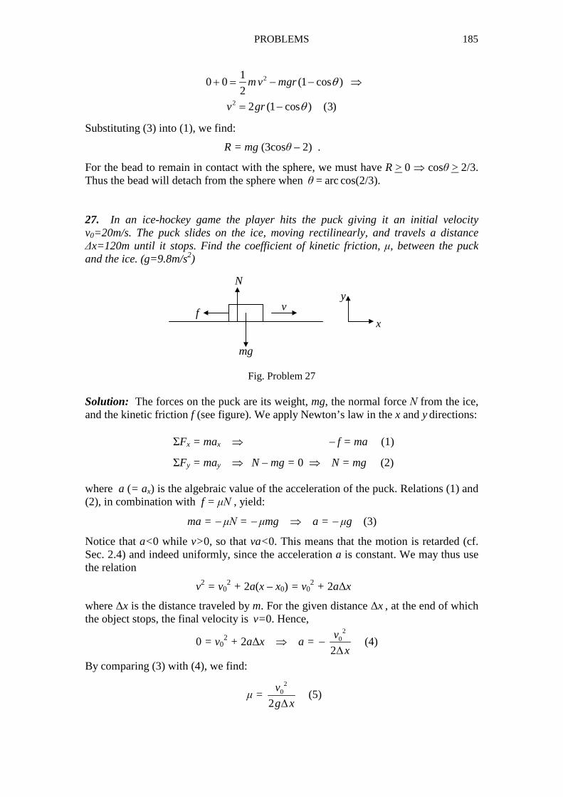
PROBLEMS 185
2
2
10 0 (1 cos )
22 (1 cos ) (3)
m v mgr
v gr
θ
θ
+ = − − ⇒
= −
Substituting (3) into (1), we find:
R = mg (3cosθ – 2) .
For the bead to remain in contact with the sphere, we must have R > 0 ⇒ cosθ > 2/3. Thus the bead will detach from the sphere when θ = arc cos(2/3). 27. In an ice-hockey game the player hits the puck giving it an initial velocity v0=20m/s. The puck slides on the ice, moving rectilinearly, and travels a distance ∆x=120m until it stops. Find the coefficient of kinetic friction, µ, between the puck and the ice. (g=9.8m/s2)
Fig. Problem 27 Solution: The forces on the puck are its weight, mg, the normal force Ν from the ice, and the kinetic friction f (see figure). We apply Newton’s law in the x and y directions: ΣFx = max ⇒ − f = ma (1)
ΣFy = may ⇒ N – mg = 0 ⇒ N = mg (2) where a (= ax) is the algebraic value of the acceleration of the puck. Relations (1) and (2), in combination with f = µΝ , yield:
ma = − µΝ = − µmg ⇒ a = − µg (3)
Notice that a<0 while v>0, so that va<0. This means that the motion is retarded (cf. Sec. 2.4) and indeed uniformly, since the acceleration a is constant. We may thus use the relation
v2 = v02 + 2a(x – x0) = v0
2 + 2a∆x
where ∆x is the distance traveled by m. For the given distance ∆x , at the end of which the object stops, the final velocity is v=0. Hence,
0 = v02 + 2a∆x ⇒ a =
20
2
v
x−
∆ (4)
By comparing (3) with (4), we find:
µ = 2
0
2
v
g x∆ (5)
mg
f
N
v
x
y

186 PROBLEMS
Alternatively, we can make use of the work-energy theorem. The forces Ν and mg do not produce work since they are normal to the velocity. Thus the total work on m is done by the friction f alone and is equal to the change of the kinetic energy of m:
∆Ek = Wf ⇒ 0 − 1
2mv0
2 = − f ∆x .
(Explain the negative sign in the expression for Wf .) We have:
1
2mv0
2 = f ∆x = µΝ ∆x = µmg∆x ⇒ µ = 2
0
2
v
g x∆ ,
which is the same as (5). Substituting for the given values, we find: µ= 0.17. 28. A cube is let to slide down form the top of an inclined plane of length l and angle of inclination θ, which plane rests on a horizontal table (see figure). There is no fric-tion between the cube and the incline, while the coefficient of kinetic friction between the cube and the table is µ. How far from the base of the incline will the cube go be-fore it stops?
i
A
B C
h
N
mgθ f
N′
mg
0v=
Fig. Problem 28 Solution: Along the path ΑΒ, of length ΑΒ=l , the cube is subject to the conservative force mg and the normal reaction Ν, which produces no work (why?). Thus, ∆(Ek+Ep) = WN = 0 ⇒ Ek+Ep = constant .
In particular, (Ek+Ep)Α = (Ek+Ep)Β . Taking Ep=0 at the base of the inclined plane, and using the fact that vA=0, we have:
0 + mgh = 1
2mvB
2 + 0 ⇒ vB 2 = 2gh = 2glsinθ (1)
Along the path BC (where C is the point at which the cube stops) only the friction f produces work (why?), which work is negative since f opposes the motion of the cube. By the work-energy theorem,
∆Ek = Ek,C – Ek,B = Wf ⇒ 0 − 1
2mvB
2 = − f (BC) ⇒
mvB 2 = 2 f (BC) = 2µΝ΄(BC) = 2µmg(BC) ⇒ vB
2 = 2µg(BC) (2)
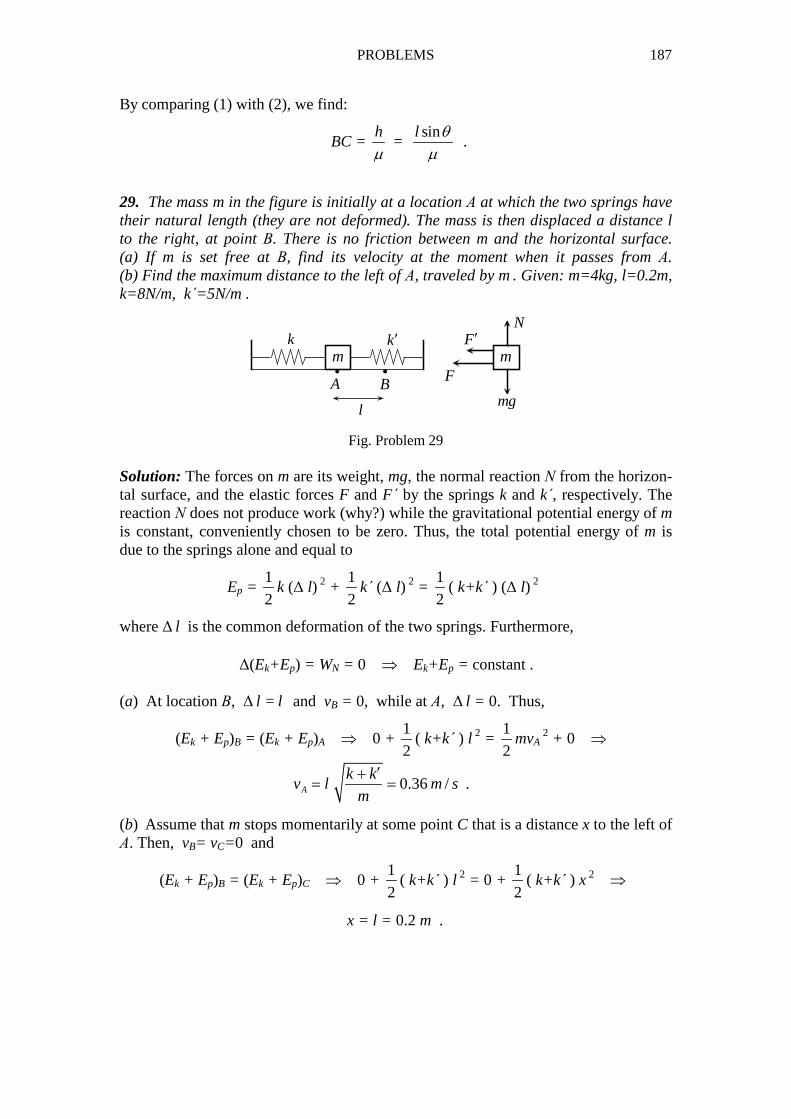
PROBLEMS 187
By comparing (1) with (2), we find:
BC = h
µ =
sinl θµ
.
29. The mass m in the figure is initially at a location Α at which the two springs have their natural length (they are not deformed). The mass is then displaced a distance l to the right, at point Β. There is no friction between m and the horizontal surface. (a) If m is set free at Β, find its velocity at the moment when it passes from Α. (b) Find the maximum distance to the left of Α, traveled by m . Given: m=4kg, l=0.2m, k=8N/m, k=5N/m .
m mi i
k k′
A B
lmg
N
F
F ′
Fig. Problem 29 Solution: The forces on m are its weight, mg, the normal reaction Ν from the horizon-tal surface, and the elastic forces F and F΄ by the springs k and k΄, respectively. The reaction Ν does not produce work (why?) while the gravitational potential energy of m is constant, conveniently chosen to be zero. Thus, the total potential energy of m is due to the springs alone and equal to
Ep = 1
2k (∆ l) 2 +
1
2k΄ (∆ l) 2 =
1
2( k+k΄ ) (∆ l) 2
where ∆ l is the common deformation of the two springs. Furthermore, ∆(Ek+Ep) = WN = 0 ⇒ Ek+Ep = constant . (a) At location Β, ∆ l = l and vB = 0, while at Α, ∆ l = 0. Thus,
(Ek + Ep)B = (Ek + Ep)A ⇒ 0 + 1
2( k+k΄ ) l 2 =
1
2mvA
2 + 0 ⇒
0.36 / .A
k kv l m s
m
′+= =
(b) Assume that m stops momentarily at some point C that is a distance x to the left of Α. Then, vB= vC=0 and
(Ek + Ep)B = (Ek + Ep)C ⇒ 0 + 1
2( k+k΄ ) l 2 = 0 +
1
2( k+k΄ ) x 2 ⇒
x = l = 0.2 m .
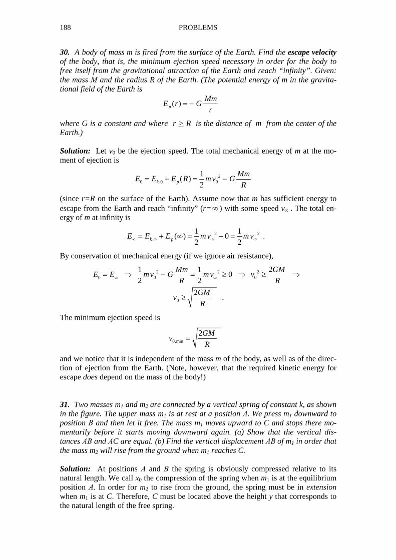
188 PROBLEMS
30. A body of mass m is fired from the surface of the Earth. Find the escape velocity of the body, that is, the minimum ejection speed necessary in order for the body to free itself from the gravitational attraction of the Earth and reach “infinity”. Given: the mass Μ and the radius R of the Earth. (The potential energy of m in the gravita-tional field of the Earth is
( )p
MmE r G
r= −
where G is a constant and where r > R is the distance of m from the center of the Earth.) Solution: Let v0 be the ejection speed. The total mechanical energy of m at the mo-ment of ejection is
20 ,0 0
1( )
2k p
MmE E E R mv G
R= + = −
(since r=R on the surface of the Earth). Assume now that m has sufficient energy to escape from the Earth and reach “infinity” (r= ∞ ) with some speed v∞ . The total en-ergy of m at infinity is
2 2,
1 1( ) 0
2 2k pE E E m v m v∞ ∞ ∞ ∞= + ∞ = + = .
By conservation of mechanical energy (if we ignore air resistance),
2 2 20 0 0
0
1 1 20
2 2
2.
Mm GME E mv G mv v
R R
GMv
R
∞ ∞= ⇒ − = ≥ ⇒ ≥ ⇒
≥
The minimum ejection speed is
0,min
2GMv
R=
and we notice that it is independent of the mass m of the body, as well as of the direc-tion of ejection from the Earth. (Note, however, that the required kinetic energy for escape does depend on the mass of the body!) 31. Two masses m1 and m2 are connected by a vertical spring of constant k, as shown in the figure. The upper mass m1 is at rest at a position Α. We press m1 downward to position Β and then let it free. The mass m1 moves upward to C and stops there mo-mentarily before it starts moving downward again. (a) Show that the vertical dis-tances ΑΒ and ΑC are equal. (b) Find the vertical displacement ΑΒ of m1 in order that the mass m2 will rise from the ground when m1 reaches C. Solution: At positions Α and Β the spring is obviously compressed relative to its natural length. We call x0 the compression of the spring when m1 is at the equilibrium position Α. In order for m2 to rise from the ground, the spring must be in extension when m1 is at C. Therefore, C must be located above the height y that corresponds to the natural length of the free spring.

PROBLEMS 189
O
y
0xA
B
C
kk
k
1m
1m
1m
2m 2m 2m
free spring
Fig. Problem 31 The equilibrium condition for m1 at point Α is
k x0 = m1 g (1)
The total mechanical energy of m1 at an arbitrary position y is
E = Ek + Ep = 1
2m1v
2 + m1 g y + 1
2k x2
where x is the deformation of the spring (compression or extension) relative to its natural length. At positions Β and C, vB=vC=0. Also, xB=x0+AB, xC=AC–x0 . By con-servation of mechanical energy, EB = EC ⇒
0 + m1 g yΒ + 1
2k (x0 + AB)2 = 0 + m1 g yC +
1
2k (AC – x0)
2 ⇒
1
2k [(x0 + AB)2 − (AC – x0)
2 ] = m1 g ( yC – yB ) = m1 g (BC) ⇒
1
2k [(AB)2 − (AC)2 ] + k x0 (AB+AC) = m1 g (BC)
or, given that AB+AC = BC ,
1
2k [(AB)2 − (AC)2 ] = (m1 g − k x0)(BC) = 0
due to (1). Thus, finally, AB = AC (2)
In order for the mass m2 to rise (even slightly), the extended spring must exert on it an upward force at least equal to its weight:
k xC > m2 g ⇒ k (AC – x0) > m2 g .
Substituting AC = AB and k x0 = m1 g, according to (1) and (2), we find:
ΑΒ > 1 2( )m m g
k
+ .

190 PROBLEMS
32. A pump raises water at a height H above a tank, at a rate of α kg/s (mass of wa-ter per unit time). The water reaches its final height having acquired a speed v. Find the work supplied per unit time by the pump.
Tank
H
1h
2h
0v =
v h
Fig. Problem 32 Solution: The heights h1 and h2 (see figure) are measured relative to an arbitrary ref-erence level. Let dm be the mass of water arriving at height h2 and, within time dt, added to the quantity of water already existing there. The rate at which water is deliv-ered at h2 is
dm
dtα= (1)
The work dW supplied by the pump within time dt is equal to the change of the total mechanical energy of dm between the levels h1 and h2 :
dW = ∆ (Ek+Ep) = (Ek+Ep)2 − (Ek+Ep)1 = [1
2(dm)v2 + (dm)gh2] – [0 + (dm)gh1] .
That is,
dW = 1
2(dm)v2 + (dm)g(h2 – h1) =
1
2(dm)v2 + (dm)gH .
The work supplied per unit time by the pump is, therefore,
(1)
21
2
dW dm dmv gH
dt dt dt= + ⇒
21
2
dWv gH
dtα α= + .
33. A particle performs simple harmonic motion on the x-axis, according to the equa-tion x = A cosωt, where ω=2π/Τ. Determine the time intervals in which the motion is accelerated or retarded. Solution: In accordance with the discussion in Sec. 2.4, we need to examine the sign of the product va, where v and a are the algebraic values of the velocity and the accel-eration, respectively. We have:
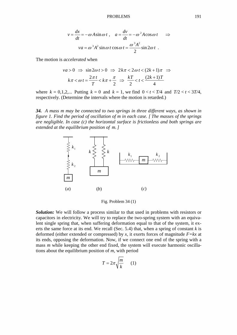
PROBLEMS 191
2sin , cosdx dv
v A t a A tdt dt
ω ω ω ω= = − = = − ⇒
3 2
3 2 sin cos sin 22
Ava A t t t
ωω ω ω ω= = .
The motion is accelerated when
0 sin 2 0 2 2 (2 1)
2 (2 1)
2 2 4
va t k t k
t kT k Tk t k t
T
ω π ω ππ π
π ω π
> ⇒ > ⇒ < < + ⇒
+< = < + ⇒ < <
where k = 0,1,2,... Putting k = 0 and k = 1, we find 0 < t < T/4 and T/2 < t < 3T/4, respectively. (Determine the intervals where the motion is retarded.)
34. A mass m may be connected to two springs in three different ways, as shown in figure 1. Find the period of oscillation of m in each case. [ The masses of the springs are negligible. In case (c) the horizontal surface is frictionless and both springs are extended at the equilibrium position of m. ]
1k
2k
m
i
m
kk1k 2k
m
( )a ( )b ( )c
Fig. Problem 34 (1)
Solution: We will follow a process similar to that used in problems with resistors or capacitors in electricity. We will try to replace the two-spring system with an equiva-lent single spring that, when suffering deformation equal to that of the system, it ex-erts the same force at its end. We recall (Sec. 5.4) that, when a spring of constant k is deformed (either extended or compressed) by x, it exerts forces of magnitude F=kx at its ends, opposing the deformation. Now, if we connect one end of the spring with a mass m while keeping the other end fixed, the system will execute harmonic oscilla-tions about the equilibrium position of m, with period
2m
Tk
π= (1)
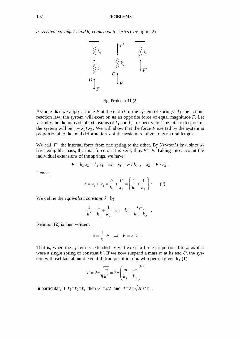
192 PROBLEMS
a. Vertical springs k1 and k2 connected in series (see figure 2)
1k
2k
i
iO
F
2k
i
iO
F
F ′
i
1k
F ′
Fig. Problem 34 (2) Assume that we apply a force F at the end Ο of the system of springs. By the action-reaction law, the system will exert on us an opposite force of equal magnitude F. Let x1 and x2 be the individual extensions of k1 and k2 , respectively. The total extension of the system will be x= x1+x2 . We will show that the force F exerted by the system is proportional to the total deformation x of the system, relative to its natural length. We call F΄ the internal force from one spring to the other. By Newton’s law, since k2 has negligible mass, the total force on it is zero; thus F΄=F . Taking into account the individual extensions of the springs, we have:
F = k2 x2 = k1 x1 ⇒ x1 = F / k1 , x2 = F / k2 .
Hence,
1 21 2 1 2
1 1F Fx x x F
k k k k
= + = + = +
(2)
We define the equivalent constant k΄ by
1 2
1 2 1 2
1 1 1 k kk΄
k΄ k k k k= + ⇔ =
+ .
Relation (2) is then written:
1
x F F k xk΄
= ⇒ = .
That is, when the system is extended by x, it exerts a force proportional to x, as if it were a single spring of constant k΄. If we now suspend a mass m at its end Ο, the sys-tem will oscillate about the equilibrium position of m with period given by (1):
1/ 2
1 2
2 2m m m
Tk΄ k k
π π
= = +
.
In particular, if k1=k2=k, then k΄=k/2 and Τ=2π 2 /m k .
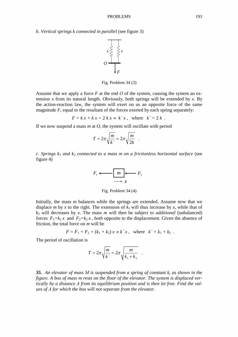
PROBLEMS 193
b. Vertical springs k connected in parallel (see figure 3)
kk
O
F
Fig. Problem 34 (3) Assume that we apply a force F at the end Ο of the system, causing the system an ex-tension x from its natural length. Obviously, both springs will be extended by x. By the action-reaction law, the system will exert on us an opposite force of the same magnitude F, equal to the resultant of the forces exerted by each spring separately:
F = k x + k x = 2 k x ≡ k x , where k΄ = 2 k .
If we now suspend a mass m at O, the system will oscillate with period
2 22
m mT
k΄ kπ π= = .
c. Springs k1 and k2 connected to a mass m on a frictionless horizontal surface (see figure 4)
m1F 2F
x
Fig. Problem 34 (4) Initially, the mass m balances while the springs are extended. Assume now that we displace m by x to the right. The extension of k1 will thus increase by x, while that of k2 will decreases by x. The mass m will then be subject to additional (unbalanced) forces F1=k1 x and F2=k2 x , both opposite to the displacement. Given the absence of friction, the total force on m will be
F = F1 + F2 = (k1 + k2) x ≡ k΄ x , where k΄ = k1 + k2 .
The period of oscillation is
1 2
2 2m m
Tk΄ k k
π π= =+
.
35. An elevator of mass Μ is suspended from a spring of constant k, as shown in the figure. A box of mass m rests on the floor of the elevator. The system is displaced ver-tically by a distance Α from its equilibrium position and is then let free. Find the val-ues of Α for which the box will not separate from the elevator.

194 PROBLEMS
Fig. Problem 35 Solution: We assume that the elevator and the box move together like a single body, with common acceleration a. The situation is thus equivalent to that of a mass (M+m) hanging from a spring k. Such a system executes harmonic oscillations about its equi-librium position, of angular frequency ω= [k /(M+m)]1/2. If y is the instantaneous dis-placement from the equilibrium position, the corresponding total force on the system has magnitude F=ky [see Sec. 5.4, equation (5.20)]. Thus, the magnitude of the in-stantaneous acceleration of the system is
F k y
aM m M m
= =+ +
.
Given that the maximum displacement equals the amplitude Α of oscillation, the maximum value of the acceleration is
max
k Aa
M m=
+ (1)
Now, the box may separate from the floor of the elevator only when the system accel-erates downward. Thus, if separation is to be avoided, the downward acceleration a of the elevator must never exceed the acceleration g of free fall of the box:
(1)
max
( )M m ga g A
k
+≤ ⇒ ≤ .
36. Consider two particles m1 and m2 subject only to their mutual interaction (iso-lated system). Call 12F
�
the force on m1 due to m2 , and 12a�
the acceleration of m1 rela-
tive to m2 . (Then, 21 12F F= −� �
and 21 12a a= −� �
.) Show that
12 12F aµ=� �
(1)
where µ is the reduced mass of the system:
1 2
1 2 1 2
1 1 1m m
m m m mµ
µ= ⇔ = +
+ .
Solution: Let 1 2,a a� �
be the accelerations of m1 , m2 , relative to an inertial frame of
reference. By Newton’s law, and given the absence of external forces, we have:
12 21 121 2
1 2 2
,F F F
a am m m
= = = −
� � �
� �
.
m
M
k
a
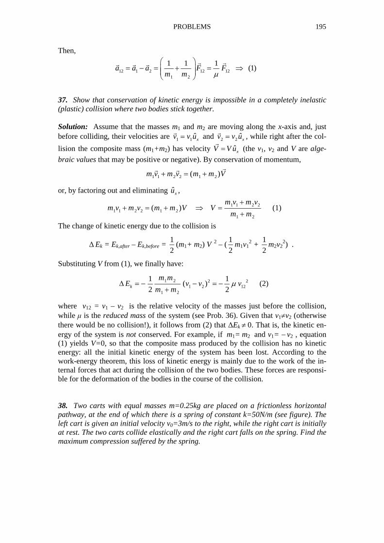
PROBLEMS 195
Then,
12 1 2 12 121 2
1 1 1(1)a a a F F
m m µ
= − = + = ⇒
� �� � �
37. Show that conservation of kinetic energy is impossible in a completely inelastic (plastic) collision where two bodies stick together. Solution: Assume that the masses m1 and m2 are moving along the x-axis and, just before colliding, their velocities are 1 1 ˆxv v u=
�
and 2 2 ˆxv v u=�
, while right after the col-
lision the composite mass (m1+m2) has velocity ˆxV V u=�
(the v1, v2 and V are alge-
braic values that may be positive or negative). By conservation of momentum,
1 1 2 2 1 2( )m v m v m m V+ = +�� �
or, by factoring out and eliminating ˆxu ,
1 1 2 21 1 2 2 1 2
1 2
( )m v m v
m v m v m m V Vm m
++ = + ⇒ =
+ (1)
The change of kinetic energy due to the collision is
∆ Ek = Ek,after – Ek,before = 1
2(m1+ m2) V
2 – (1
2m1v1
2 + 1
2m2v2
2) .
Substituting V from (1), we finally have:
1 2 2 21 2 12
1 2
1 1( )
2 2k
m mE v v v
m mµ∆ = − − = −
+ (2)
where v12 = v1 – v2 is the relative velocity of the masses just before the collision, while µ is the reduced mass of the system (see Prob. 36). Given that v1≠v2 (otherwise there would be no collision!), it follows from (2) that ∆Ek ≠ 0. That is, the kinetic en-ergy of the system is not conserved. For example, if m1= m2 and v1= − v2 , equation (1) yields V=0, so that the composite mass produced by the collision has no kinetic energy: all the initial kinetic energy of the system has been lost. According to the work-energy theorem, this loss of kinetic energy is mainly due to the work of the in-ternal forces that act during the collision of the two bodies. These forces are responsi-ble for the deformation of the bodies in the course of the collision. 38. Two carts with equal masses m=0.25kg are placed on a frictionless horizontal pathway, at the end of which there is a spring of constant k=50N/m (see figure). The left cart is given an initial velocity v0=3m/s to the right, while the right cart is initially at rest. The two carts collide elastically and the right cart falls on the spring. Find the maximum compression suffered by the spring.
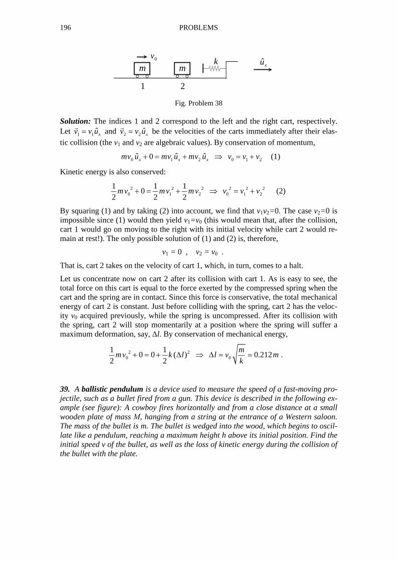
196 PROBLEMS
m� �
m� �
0v
1 2
k ˆxu
Fig. Problem 38 Solution: The indices 1 and 2 correspond to the left and the right cart, respectively. Let 1 1 ˆxv v u=�
and 2 2 ˆxv v u=�
be the velocities of the carts immediately after their elas-
tic collision (the v1 and v2 are algebraic values). By conservation of momentum,
0 1 2 0 1 2ˆ ˆ ˆ0x x xmv u mv u mv u v v v+ = + ⇒ = + (1)
Kinetic energy is also conserved:
2 2 2 2 2 20 1 2 0 1 2
1 1 10
2 2 2mv mv mv v v v+ = + ⇒ = + (2)
By squaring (1) and by taking (2) into account, we find that v1v2=0. The case v2=0 is impossible since (1) would then yield v1=v0 (this would mean that, after the collision, cart 1 would go on moving to the right with its initial velocity while cart 2 would re-main at rest!). The only possible solution of (1) and (2) is, therefore,
v1 = 0 , v2 = v0 .
That is, cart 2 takes on the velocity of cart 1, which, in turn, comes to a halt.
Let us concentrate now on cart 2 after its collision with cart 1. As is easy to see, the total force on this cart is equal to the force exerted by the compressed spring when the cart and the spring are in contact. Since this force is conservative, the total mechanical energy of cart 2 is constant. Just before colliding with the spring, cart 2 has the veloc-ity v0 acquired previously, while the spring is uncompressed. After its collision with the spring, cart 2 will stop momentarily at a position where the spring will suffer a maximum deformation, say, ∆l. By conservation of mechanical energy,
2 20 0
1 10 0 ( ) 0.212 .
2 2
mmv k l l v m
k+ = + ∆ ⇒ ∆ = ≃
39. A ballistic pendulum is a device used to measure the speed of a fast-moving pro-jectile, such as a bullet fired from a gun. This device is described in the following ex-ample (see figure): A cowboy fires horizontally and from a close distance at a small wooden plate of mass Μ, hanging from a string at the entrance of a Western saloon. The mass of the bullet is m. The bullet is wedged into the wood, which begins to oscil-late like a pendulum, reaching a maximum height h above its initial position. Find the initial speed v of the bullet, as well as the loss of kinetic energy during the collision of the bullet with the plate.
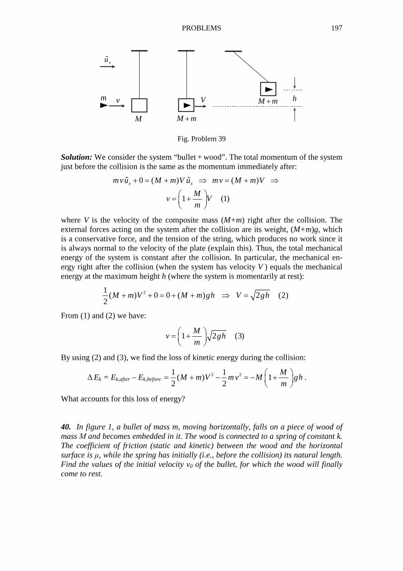
PROBLEMS 197
ˆxu
vm
M
V
M m+
M m+ h
Fig. Problem 39 Solution: We consider the system “bullet + wood”. The total momentum of the system just before the collision is the same as the momentum immediately after:
ˆ ˆ0 ( ) ( )
1 (1)
x xmvu M m V u mv M m V
Mv V
m
+ = + ⇒ = + ⇒
= +
where V is the velocity of the composite mass (M+m) right after the collision. The external forces acting on the system after the collision are its weight, (M+m)g, which is a conservative force, and the tension of the string, which produces no work since it is always normal to the velocity of the plate (explain this). Thus, the total mechanical energy of the system is constant after the collision. In particular, the mechanical en-ergy right after the collision (when the system has velocity V ) equals the mechanical energy at the maximum height h (where the system is momentarily at rest):
21( ) 0 0 ( ) 2 (2)
2M m V M m gh V gh+ + = + + ⇒ =
From (1) and (2) we have:
1 2 (3)M
v ghm
= +
By using (2) and (3), we find the loss of kinetic energy during the collision:
∆ Ek = Ek,after – Ek,before 2 21 1
( ) 12 2
MM m V mv M gh
m = + − = − +
.
What accounts for this loss of energy? 40. In figure 1, a bullet of mass m, moving horizontally, falls on a piece of wood of mass Μ and becomes embedded in it. The wood is connected to a spring of constant k. The coefficient of friction (static and kinetic) between the wood and the horizontal surface is µ, while the spring has initially (i.e., before the collision) its natural length. Find the values of the initial velocity v0 of the bullet, for which the wood will finally come to rest.
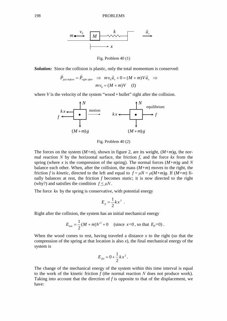
198 PROBLEMS
0v k ˆxum M•
x
Fig. Problem 40 (1)
Solution: Since the collision is plastic, only the total momentum is conserved:
0
0
ˆ ˆ0 ( )
( ) (1)
just before right after x xP P mv u M m V u
mv M m V
= ⇒ + = + ⇒
= +
� �
where V is the velocity of the system “wood + bullet” right after the collision.
•
N
( )M m g+
•
N
( )M m g+
f fk xk x motion
equilibrium
Fig. Problem 40 (2) The forces on the system (M+m), shown in figure 2, are its weight, (M+m)g, the nor-mal reaction Ν by the horizontal surface, the friction f, and the force kx from the spring (where x is the compression of the spring). The normal forces (M+m)g and Ν balance each other. When, after the collision, the mass (M+m) moves to the right, the friction f is kinetic, directed to the left and equal to f = µN = µ(M+m)g. If (M+m) fi-nally balances at rest, the friction f becomes static; it is now directed to the right (why?) and satisfies the condition f < µΝ .
The force kx by the spring is conservative, with potential energy
21
2pE k x= .
Right after the collision, the system has an initial mechanical energy
21( ) 0
2initE M m V= + + (since x=0 , so that Ep=0) .
When the wood comes to rest, having traveled a distance x to the right (so that the compression of the spring at that location is also x), the final mechanical energy of the system is
210
2finE k x= + .
The change of the mechanical energy of the system within this time interval is equal to the work of the kinetic friction f (the normal reaction Ν does not produce work). Taking into account that the direction of f is opposite to that of the displacement, we have:
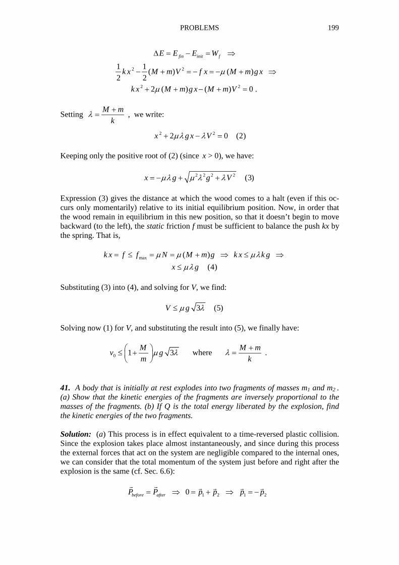
PROBLEMS 199
2 2
2 2
1 1( ) ( )
2 22 ( ) ( ) 0 .
fin init fE E E W
k x M m V f x M m g x
k x M m g x M m V
µ
µ
∆ = − = ⇒
− + = − = − + ⇒
+ + − + =
Setting M m
kλ
+= , we write:
2 22 0 (2)x g x Vµλ λ+ − = Keeping only the positive root of (2) (since x > 0), we have:
2 2 2 2 (3)x g g Vµλ µ λ λ= − + +
Expression (3) gives the distance at which the wood comes to a halt (even if this oc-curs only momentarily) relative to its initial equilibrium position. Now, in order that the wood remain in equilibrium in this new position, so that it doesn’t begin to move backward (to the left), the static friction f must be sufficient to balance the push kx by the spring. That is,
max ( )
(4)
k x f f N M m g k x k g
x g
µ µ µλ
µλ
= ≤ = = + ⇒ ≤ ⇒
≤
Substituting (3) into (4), and solving for V, we find:
3 (5)V gµ λ≤ Solving now (1) for V, and substituting the result into (5), we finally have:
0 1 3M
v gm
µ λ ≤ +
where M m
kλ
+= .
41. A body that is initially at rest explodes into two fragments of masses m1 and m2 . (a) Show that the kinetic energies of the fragments are inversely proportional to the masses of the fragments. (b) If Q is the total energy liberated by the explosion, find the kinetic energies of the two fragments. Solution: (a) This process is in effect equivalent to a time-reversed plastic collision. Since the explosion takes place almost instantaneously, and since during this process the external forces that act on the system are negligible compared to the internal ones, we can consider that the total momentum of the system just before and right after the explosion is the same (cf. Sec. 6.6):
1 2 1 20before afterP P p p p p= ⇒ = + ⇒ = −� � � � � �
200 PROBLEMS
where 1p�
and 2p�
are the momenta of the two fragments. If p1 and p2 are the magni-
tudes of the momenta, then p1= p2 ≡ p . Now, in general, the kinetic energy of a body of mass m and momentum p is equal to
2
2k
pE
m= .
Hence,
2 2 2 2
1 2,1 ,2
1 1 2 2
,2 2 2 2k k
p p p pE E
m m m m= = = =
and, by dividing these relations,
2,1
,2 1
(1)k
k
mE
E m=
(b) Assume now that
Ek,1 + Ek,2 = Q . By applying a well-known property of proportions to (1), we have:
2 1 2,1 ,1 ,2
,1 ,2 1 2 ,2 1
,k k k
k k k
m m mE E E
E E m m E m
++= =
+ + .
Thus,
2 1,1 ,2
1 2 1 2
,k k
m mE Q E Q
m m m m= =
+ + .
Notice that, if m1<< m2 , then Ek,2 ≈ 0 and Ek,1 ≈ Q . That is, almost all of the liber-ated energy Q goes off as kinetic energy of the smaller fragment. This is what hap-pens, for example, in a radioactive decay of an atomic nucleus.
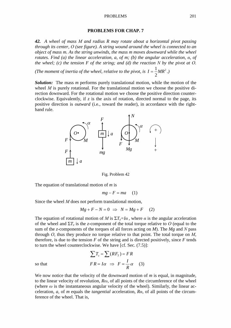
PROBLEMS 201
PROBLEMS FOR CHAP. 7 42. A wheel of mass Μ and radius R may rotate about a horizontal pivot passing through its center, Ο (see figure). A string wound around the wheel is connected to an object of mass m. As the string unwinds, the mass m moves downward while the wheel rotates. Find (a) the linear acceleration, a, of m; (b) the angular acceleration, α, of the wheel; (c) the tension F of the string; and (d) the reaction Ν by the pivot at Ο.
(The moment of inertia of the wheel, relative to the pivot, is 21
2I MR= .)
Solution: The mass m performs purely translational motion, while the motion of the wheel Μ is purely rotational. For the translational motion we choose the positive di-rection downward. For the rotational motion we choose the positive direction counter-clockwise. Equivalently, if z is the axis of rotation, directed normal to the page, its positive direction is outward (i.e., toward the reader), in accordance with the right-hand rule.
i m i
m
+
+
M M
O O
F
F
F
F
mgMg
N
a
a
αα
Fig. Problem 42 The equation of translational motion of m is
mg F ma− = (1)
Since the wheel Μ does not perform translational motion,
0Mg F N N Mg F+ − = ⇒ = + (2)
The equation of rotational motion of Μ is ΣTz=Iα , where α is the angular acceleration of the wheel and ΣTz is the z-component of the total torque relative to Ο (equal to the sum of the z-components of the torques of all forces acting on M). The Mg and Ν pass through Ο, thus they produce no torque relative to that point. The total torque on Μ, therefore, is due to the tension F of the string and is directed positively, since F tends to turn the wheel counterclockwise. We have [cf. Sec. (7.5)]:
( )z TT RF F R= =∑ ∑
so that I
F R I FR
α α= ⇒ = (3)
We now notice that the velocity of the downward motion of m is equal, in magnitude, to the linear velocity of revolution, Rω, of all points of the circumference of the wheel (where ω is the instantaneous angular velocity of the wheel). Similarly, the linear ac-celeration, a, of m equals the tangential acceleration, Rα, of all points of the circum-ference of the wheel. That is,
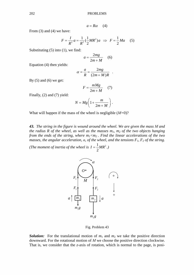
202 PROBLEMS
a Rα= (4) From (3) and (4) we have:
22 2
1 1 1( )2 2
IF a MR a F Ma
R R= = ⇒ = (5)
Substituting (5) into (1), we find:
2
2
mga
m M=
+ (6)
Equation (4) then yields:
2
(2 )
a mg
R m M Rα = =
+ .
By (5) and (6) we get:
2
mMgF
m M=
+ (7)
Finally, (2) and (7) yield:
12
mN Mg
m M = + +
.
What will happen if the mass of the wheel is negligible (Μ=0)? 43. The string in the figure is wound around the wheel. We are given the mass Μ and the radius R of the wheel, as well as the masses m1, m2 of the two objects hanging from the ends of the string, where m1<m2 . Find the linear accelerations of the two masses, the angular acceleration, α, of the wheel, and the tensions F1, F2 of the string.
(The moment of inertia of the wheel is 21
2I MR= .)
i
1m2m
α
a a
O
M1F
1F
2F
2F
1m g
2m g
+
+
Fig. Problem 43 Solution: For the translational motion of m1 and m2 we take the positive direction downward. For the rotational motion of Μ we choose the positive direction clockwise. That is, we consider that the z-axis of rotation, which is normal to the page, is posi-
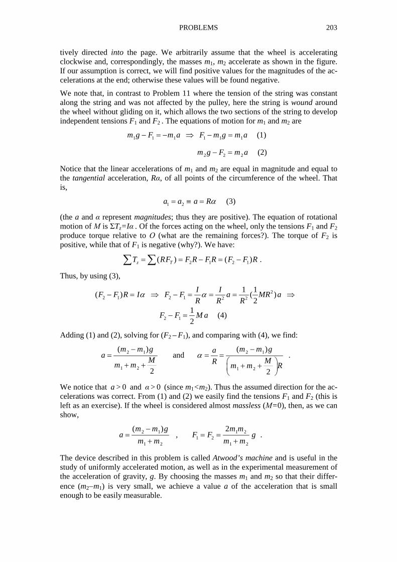
PROBLEMS 203
tively directed into the page. We arbitrarily assume that the wheel is accelerating clockwise and, correspondingly, the masses m1, m2 accelerate as shown in the figure. If our assumption is correct, we will find positive values for the magnitudes of the ac-celerations at the end; otherwise these values will be found negative.
We note that, in contrast to Problem 11 where the tension of the string was constant along the string and was not affected by the pulley, here the string is wound around the wheel without gliding on it, which allows the two sections of the string to develop independent tensions F1 and F2 . The equations of motion for m1 and m2 are
1 1 1 1 1 1m g F m a F m g m a− = − ⇒ − = (1)
2 2 2m g F m a− = (2)
Notice that the linear accelerations of m1 and m2 are equal in magnitude and equal to the tangential acceleration, Rα, of all points of the circumference of the wheel. That is,
1 2a a a Rα= ≡ = (3)
(the a and α represent magnitudes; thus they are positive). The equation of rotational motion of Μ is ΣTz=Iα . Of the forces acting on the wheel, only the tensions F1 and F2 produce torque relative to Ο (what are the remaining forces?). The torque of F2 is positive, while that of F1 is negative (why?). We have:
2 1 2 1( ) ( ) .z TT RF F R F R F F R= = − = −∑ ∑
Thus, by using (3),
22 1 2 1 2 2
1 1( ) ( )
2
I IF F R I F F a MR a
R R Rα α− = ⇒ − = = = ⇒
2 1
1
2F F M a− = (4)
Adding (1) and (2), solving for (F2 – F1), and comparing with (4), we find:
2 1
1 2
( )
2
m m ga
Mm m
−=
+ + and 2 1
1 2
( )
2
m m gaMR m m R
α−
= = + +
.
We notice that a > 0 and α > 0 (since m1<m2). Thus the assumed direction for the ac-celerations was correct. From (1) and (2) we easily find the tensions F1 and F2 (this is left as an exercise). If the wheel is considered almost massless (Μ=0), then, as we can show,
2 1 1 21 2
1 2 1 2
( ) 2,
m m g m ma F F g
m m m m
−= = =
+ +.
The device described in this problem is called Atwood’s machine and is useful in the study of uniformly accelerated motion, as well as in the experimental measurement of the acceleration of gravity, g. By choosing the masses m1 and m2 so that their differ-ence (m2−m1) is very small, we achieve a value a of the acceleration that is small enough to be easily measurable.
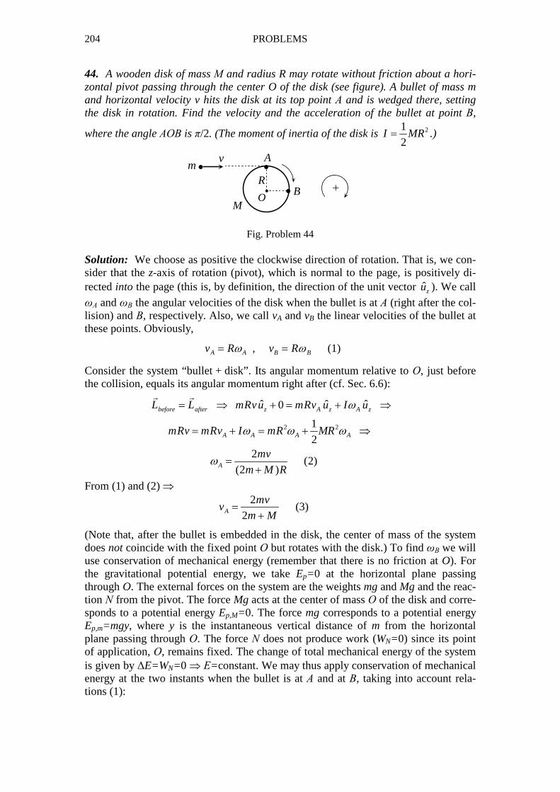
204 PROBLEMS
44. A wooden disk of mass Μ and radius R may rotate without friction about a hori-zontal pivot passing through the center O of the disk (see figure). A bullet of mass m and horizontal velocity v hits the disk at its top point Α and is wedged there, setting the disk in rotation. Find the velocity and the acceleration of the bullet at point Β,
where the angle ΑΟΒ is π/2. (The moment of inertia of the disk is 21
2I MR= .)
••
•i
mv A
BO
R
M
+
Fig. Problem 44 Solution: We choose as positive the clockwise direction of rotation. That is, we con-sider that the z-axis of rotation (pivot), which is normal to the page, is positively di-rected into the page (this is, by definition, the direction of the unit vector zu ). We call
ωΑ and ωΒ the angular velocities of the disk when the bullet is at Α (right after the col-lision) and Β, respectively. Also, we call vA and vB the linear velocities of the bullet at these points. Obviously,
,A A B Bv R v Rω ω= = (1)
Consider the system “bullet + disk”. Its angular momentum relative to Ο, just before the collision, equals its angular momentum right after (cf. Sec. 6.6):
2 2
ˆ ˆ ˆ0
1
22
(2)(2 )
before after z A z A z
A A A A
A
L L mRvu mRv u I u
mRv mRv I mR MR
mv
m M R
ω
ω ω ω
ω
= ⇒ + = + ⇒
= + = + ⇒
=+
� �
From (1) and (2) ⇒
2
2A
mvv
m M=
+ (3)
(Note that, after the bullet is embedded in the disk, the center of mass of the system does not coincide with the fixed point Ο but rotates with the disk.) To find ωΒ we will use conservation of mechanical energy (remember that there is no friction at O). For the gravitational potential energy, we take Ep=0 at the horizontal plane passing through O. The external forces on the system are the weights mg and Mg and the reac-tion Ν from the pivot. The force Mg acts at the center of mass Ο of the disk and corre-sponds to a potential energy Ep,M=0. The force mg corresponds to a potential energy Ep,m=mgy, where y is the instantaneous vertical distance of m from the horizontal plane passing through Ο. The force Ν does not produce work (WN=0) since its point of application, Ο, remains fixed. The change of total mechanical energy of the system is given by ∆E=WN=0 ⇒ Ε=constant. We may thus apply conservation of mechanical energy at the two instants when the bullet is at Α and at Β, taking into account rela-tions (1):
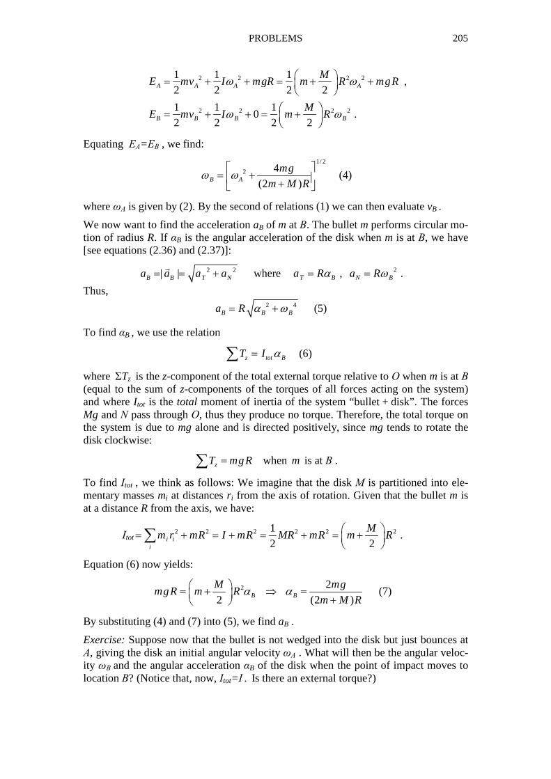
PROBLEMS 205
2 2 2 2
2 2 2 2
1 1 1,
2 2 2 2
1 1 10 .
2 2 2 2
A A A A
B B B B
ME mv I mgR m R mgR
ME mv I m R
ω ω
ω ω
= + + = + +
= + + = +
Equating ΕΑ=ΕΒ , we find:
1/ 2
2 4
(2 )B A
mg
m M Rω ω
= + +
(4)
where ωΑ is given by (2). By the second of relations (1) we can then evaluate vB .
We now want to find the acceleration aB of m at Β. The bullet m performs circular mo-tion of radius R. If αB is the angular acceleration of the disk when m is at Β, we have [see equations (2.36) and (2.37)]:
2 2| |B B T Na a a a= = +�
where 2, .T B N Ba R a Rα ω= =
Thus,
2 4B B Ba R α ω= + (5)
To find αB , we use the relation
z tot BT I α=∑ (6)
where ΣTz is the z-component of the total external torque relative to Ο when m is at Β (equal to the sum of z-components of the torques of all forces acting on the system) and where Itot is the total moment of inertia of the system “bullet + disk”. The forces Mg and Ν pass through Ο, thus they produce no torque. Therefore, the total torque on the system is due to mg alone and is directed positively, since mg tends to rotate the disk clockwise:
zT mgR=∑ when m is at Β .
To find Ιtot , we think as follows: We imagine that the disk Μ is partitioned into ele-mentary masses mi at distances r i from the axis of rotation. Given that the bullet m is at a distance R from the axis, we have:
Ιtot2 2 2 2 2 21
.2 2i i
i
Mm r mR I mR MR mR m R = + = + = + = +
∑
Equation (6) now yields:
2 2
2 (2 )B B
M mgmgR m R
m M Rα α = + ⇒ = +
(7)
By substituting (4) and (7) into (5), we find aB .
Exercise: Suppose now that the bullet is not wedged into the disk but just bounces at Α, giving the disk an initial angular velocity ωΑ . What will then be the angular veloc-ity ωΒ and the angular acceleration αB of the disk when the point of impact moves to location Β? (Notice that, now, Ιtot=Ι . Is there an external torque?)
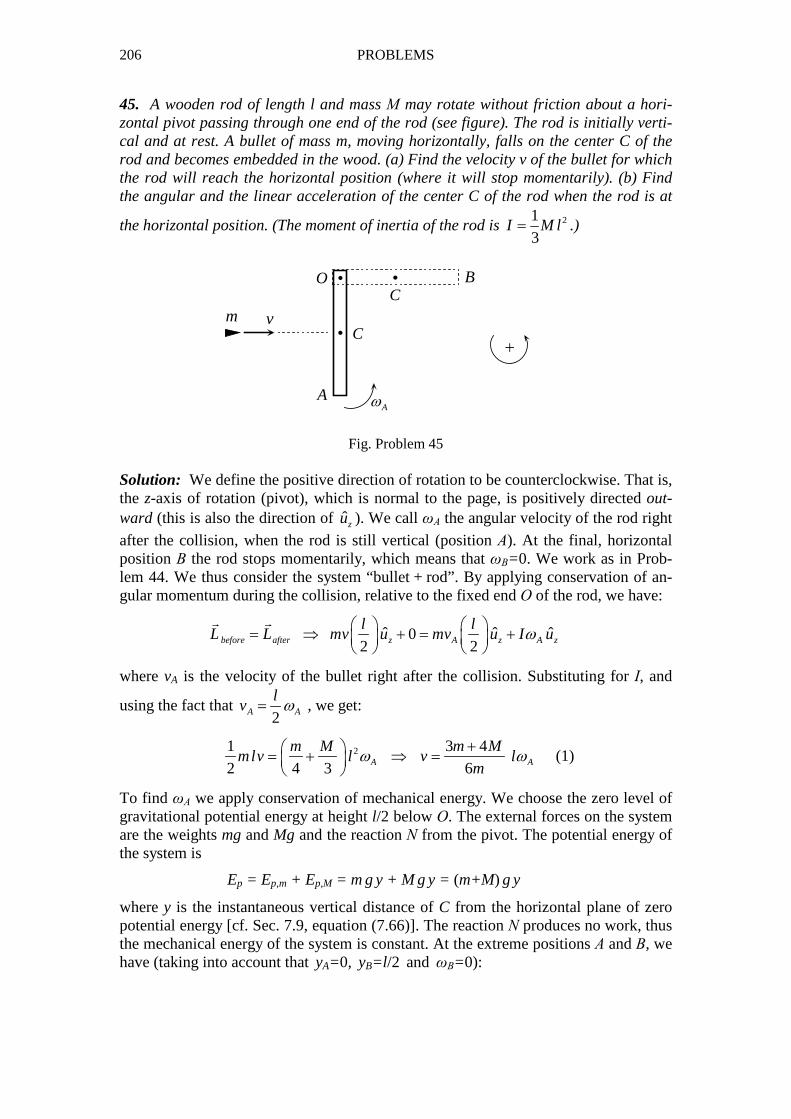
206 PROBLEMS
45. A wooden rod of length l and mass Μ may rotate without friction about a hori-zontal pivot passing through one end of the rod (see figure). The rod is initially verti-cal and at rest. A bullet of mass m, moving horizontally, falls on the center C of the rod and becomes embedded in the wood. (a) Find the velocity v of the bullet for which the rod will reach the horizontal position (where it will stop momentarily). (b) Find the angular and the linear acceleration of the center C of the rod when the rod is at
the horizontal position. (The moment of inertia of the rod is 21
3I M l= .)
i i
ii
m vC
A
BC
O
+
Aω
Fig. Problem 45 Solution: We define the positive direction of rotation to be counterclockwise. That is, the z-axis of rotation (pivot), which is normal to the page, is positively directed out-ward (this is also the direction of ˆzu ). We call ωΑ the angular velocity of the rod right
after the collision, when the rod is still vertical (position Α). At the final, horizontal position Β the rod stops momentarily, which means that ωΒ=0. We work as in Prob-lem 44. We thus consider the system “bullet + rod”. By applying conservation of an-gular momentum during the collision, relative to the fixed end Ο of the rod, we have:
ˆ ˆ ˆ02 2before after z A z A z
l lL L mv u mv u I uω = ⇒ + = +
� �
where vA is the velocity of the bullet right after the collision. Substituting for Ι, and
using the fact that 2A A
lv ω= , we get:
21 3 4
2 4 3 6A A
m M m Mmlv l v l
mω ω
+ = + ⇒ =
(1)
To find ωΑ we apply conservation of mechanical energy. We choose the zero level of gravitational potential energy at height l/2 below Ο. The external forces on the system are the weights mg and Mg and the reaction Ν from the pivot. The potential energy of the system is
Ep = Ep,m + Ep,M = m g y + M g y = (m+M) g y
where y is the instantaneous vertical distance of C from the horizontal plane of zero potential energy [cf. Sec. 7.9, equation (7.66)]. The reaction Ν produces no work, thus the mechanical energy of the system is constant. At the extreme positions Α and Β, we have (taking into account that yA=0, yB=l /2 and ωΒ=0):
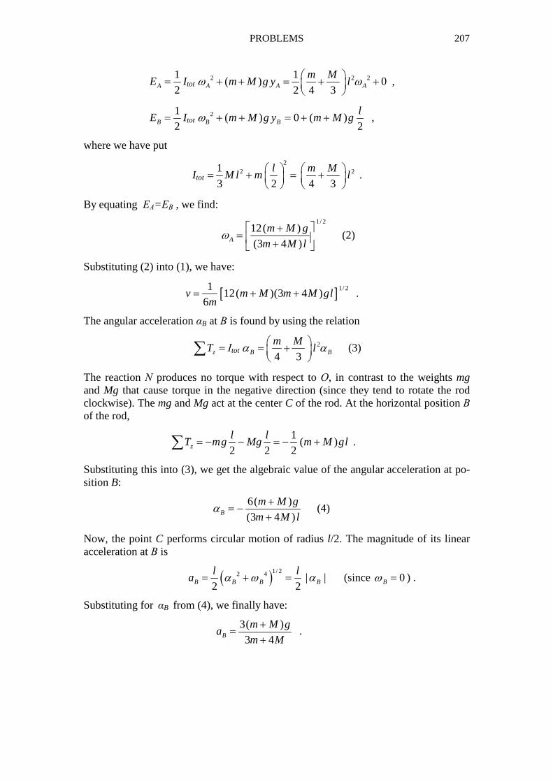
PROBLEMS 207
1
2AE = Itot 2 2 21
( ) 0 ,2 4 3A A A
m Mm M g y lω ω + + = + +
1
2BE = Itot 2 ( )B Bm M g yω + + 0 ( )
2
lm M g= + + ,
where we have put
Itot
22 21
3 2 4 3
l m MM l m l
= + = +
.
By equating ΕΑ=ΕΒ , we find:
1/ 2
12( )
(3 4 )A
m M g
m M lω
+= +
(2)
Substituting (2) into (1), we have:
[ ] 1/ 2112( )(3 4 )
6v m M m M gl
m= + + .
The angular acceleration αB at Β is found by using the relation
zT =∑ Ιtot 2
4 3B B
m Mlα α = +
(3)
The reaction Ν produces no torque with respect to Ο, in contrast to the weights mg and Mg that cause torque in the negative direction (since they tend to rotate the rod clockwise). The mg and Mg act at the center C of the rod. At the horizontal position Β of the rod,
1
( )2 2 2z
l lT mg Mg m M gl= − − = − +∑ .
Substituting this into (3), we get the algebraic value of the angular acceleration at po-sition B:
6( )
(3 4 )B
m M g
m M lα
+= −
+ (4)
Now, the point C performs circular motion of radius l/2. The magnitude of its linear acceleration at Β is
( )1/ 22 4 | |2 2B B B B
l la α ω α= + = (since 0Bω = ) .
Substituting for αB from (4), we finally have:
3( )
3 4B
m M ga
m M
+=
+ .
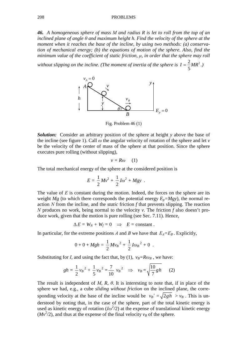
208 PROBLEMS
46. A homogeneous sphere of mass Μ and radius R is let to roll from the top of an inclined plane of angle θ and maximum height h. Find the velocity of the sphere at the moment when it reaches the base of the incline, by using two methods: (a) conserva-tion of mechanical energy; (b) the equations of motion of the sphere. Also, find the minimum value of the coefficient of static friction, µ, in order that the sphere may roll
without slipping on the incline. (The moment of inertia of the sphere is 22
5I MR= .)
hy
θ
A
B
y
0pE =
0Av =
v
Bv
Fig. Problem 46 (1) Solution: Consider an arbitrary position of the sphere at height y above the base of the incline (see figure 1). Call ω the angular velocity of rotation of the sphere and let v be the velocity of the center of mass of the sphere at that position. Since the sphere executes pure rolling (without slipping),
v = Rω (1)
The total mechanical energy of the sphere at the considered position is
E = 1
2Mv2 +
1
2Ιω
2 + Mgy .
The value of Ε is constant during the motion. Indeed, the forces on the sphere are its weight Mg (to which there corresponds the potential energy Ep=Mgy), the normal re-action Ν from the incline, and the static friction f that prevents slipping. The reaction Ν produces no work, being normal to the velocity v. The friction f also doesn’t pro-duce work, given that the motion is pure rolling (see Sec. 7.11). Hence,
∆ Ε = WN + Wf = 0 ⇒ E = constant .
In particular, for the extreme positions Α and Β we have that ΕΑ=ΕΒ . Explicitly,
0 + 0 + Mgh = 1
2MvB
2 + 1
2ΙωB
2 + 0 .
Substituting for Ι, and using the fact that, by (1), vB=RωΒ , we have:
gh = 1
2vB
2 + 1
5vB
2 =7
10 vB
2 ⇒ vB =
10
7gh (2)
The result is independent of Μ, R, θ. It is interesting to note that, if in place of the sphere we had, e.g., a cube sliding without friction on the inclined plane, the corre-
sponding velocity at the base of the incline would be vB΄ = 2gh > vB . This is un-
derstood by noting that, in the case of the sphere, part of the total kinetic energy is used as kinetic energy of rotation (Ιω
2/2) at the expense of translational kinetic energy (Mv2/2), and thus at the expense of the final velocity vB of the sphere.
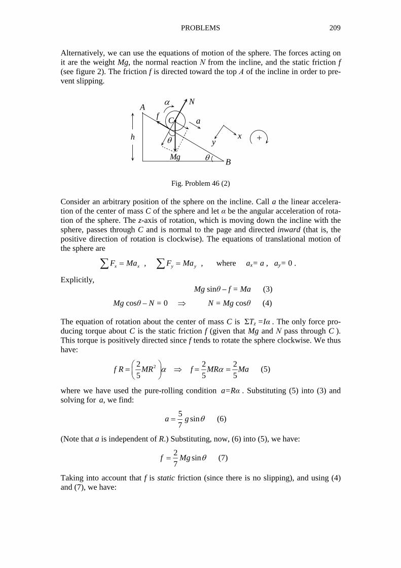
PROBLEMS 209
Alternatively, we can use the equations of motion of the sphere. The forces acting on it are the weight Mg, the normal reaction Ν from the incline, and the static friction f (see figure 2). The friction f is directed toward the top Α of the incline in order to pre-vent slipping.
i
θ
θh
A
B
C a
α
Mg
f
N
xy +
Fig. Problem 46 (2) Consider an arbitrary position of the sphere on the incline. Call a the linear accelera-tion of the center of mass C of the sphere and let α be the angular acceleration of rota-tion of the sphere. The z-axis of rotation, which is moving down the incline with the sphere, passes through C and is normal to the page and directed inward (that is, the positive direction of rotation is clockwise). The equations of translational motion of the sphere are
, ,x x y yF Ma F Ma= =∑ ∑ where ax= a , ay= 0 .
Explicitly, Mg sinθ – f = Ma (3)
Mg cosθ – N = 0 ⇒ N = Mg cosθ (4) The equation of rotation about the center of mass C is ΣTz =Iα . The only force pro-ducing torque about C is the static friction f (given that Mg and Ν pass through C ). This torque is positively directed since f tends to rotate the sphere clockwise. We thus have:
22 2 2
5 5 5f R MR f MR Maα α = ⇒ = =
(5)
where we have used the pure-rolling condition a=Rα . Substituting (5) into (3) and solving for a, we find:
5
sin7
a g θ= (6)
(Note that a is independent of R.) Substituting, now, (6) into (5), we have:
2
sin7
f Mg θ= (7)
Taking into account that f is static friction (since there is no slipping), and using (4) and (7), we have:
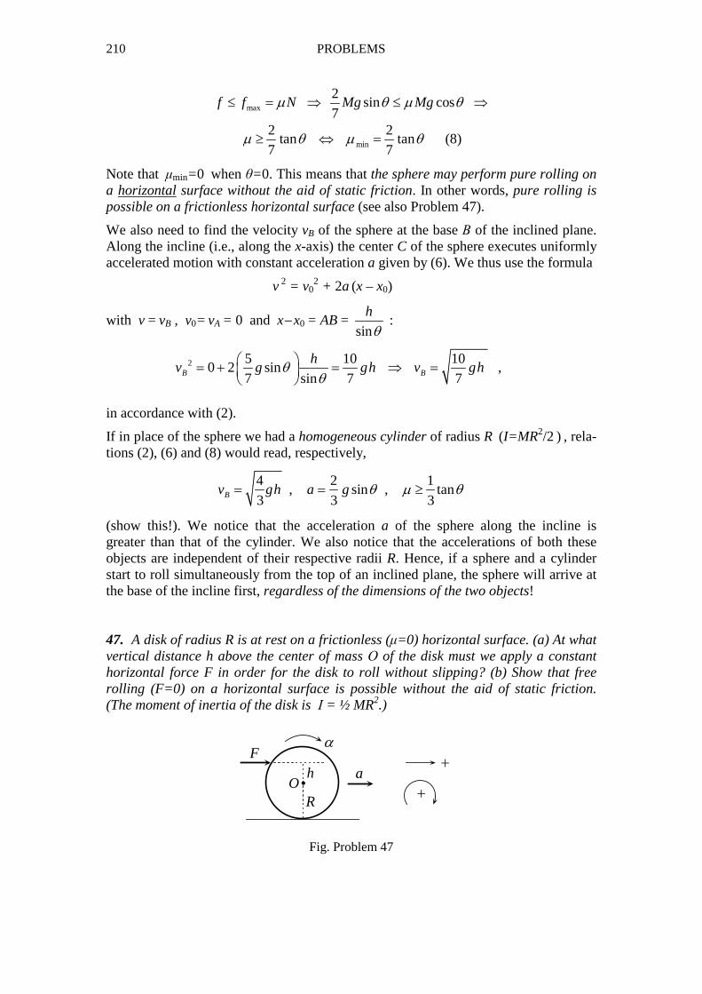
210 PROBLEMS
max
2sin cos
7f f N Mg Mgµ θ µ θ≤ = ⇒ ≤ ⇒
min
2 2tan tan
7 7µ θ µ θ≥ ⇔ = (8)
Note that µmin=0 when θ=0. This means that the sphere may perform pure rolling on a horizontal surface without the aid of static friction. In other words, pure rolling is possible on a frictionless horizontal surface (see also Problem 47).
We also need to find the velocity vB of the sphere at the base Β of the inclined plane. Along the incline (i.e., along the x-axis) the center C of the sphere executes uniformly accelerated motion with constant acceleration a given by (6). We thus use the formula
v 2 = v02 + 2a (x – x0)
with v = vB , v0= vA = 0 and x− x0 = AB = sin
h
θ :
2 5 10 100 2 sin
7 sin 7 7B B
hv g gh v ghθ
θ = + = ⇒ =
,
in accordance with (2).
If in place of the sphere we had a homogeneous cylinder of radius R (I=MR2/2 ) , rela-tions (2), (6) and (8) would read, respectively,
4 2 1
, sin , tan3 3 3Bv gh a g θ µ θ= = ≥
(show this!). We notice that the acceleration a of the sphere along the incline is greater than that of the cylinder. We also notice that the accelerations of both these objects are independent of their respective radii R. Hence, if a sphere and a cylinder start to roll simultaneously from the top of an inclined plane, the sphere will arrive at the base of the incline first, regardless of the dimensions of the two objects! 47. A disk of radius R is at rest on a frictionless (µ=0) horizontal surface. (a) At what vertical distance h above the center of mass Ο of the disk must we apply a constant horizontal force F in order for the disk to roll without slipping? (b) Show that free rolling (F=0) on a horizontal surface is possible without the aid of static friction. (The moment of inertia of the disk is Ι = ½ MR2.)
iOh
R
Fα
a+
+
Fig. Problem 47
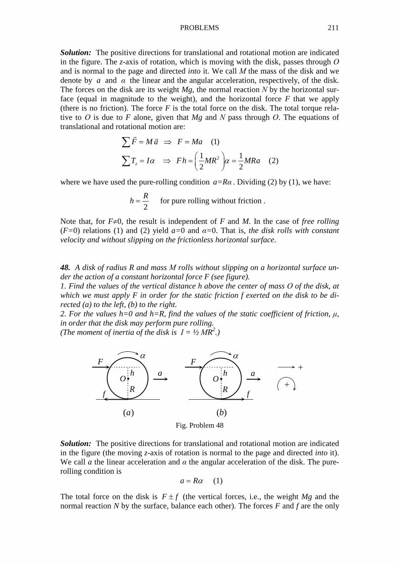
PROBLEMS 211
Solution: The positive directions for translational and rotational motion are indicated in the figure. The z-axis of rotation, which is moving with the disk, passes through Ο and is normal to the page and directed into it. We call Μ the mass of the disk and we denote by a and α the linear and the angular acceleration, respectively, of the disk. The forces on the disk are its weight Mg, the normal reaction Ν by the horizontal sur-face (equal in magnitude to the weight), and the horizontal force F that we apply (there is no friction). The force F is the total force on the disk. The total torque rela-tive to Ο is due to F alone, given that Mg and Ν pass through Ο. The equations of translational and rotational motion are:
2
(1)
1 1(2)
2 2z
F M a F Ma
T I Fh MR MRaα α
= ⇒ =
= ⇒ = =
∑
∑
� �
where we have used the pure-rolling condition a=Rα . Dividing (2) by (1), we have:
2
Rh = for pure rolling without friction .
Note that, for F≠0, the result is independent of F and M. In the case of free rolling (F=0) relations (1) and (2) yield a=0 and α=0. That is, the disk rolls with constant velocity and without slipping on the frictionless horizontal surface. 48. A disk of radius R and mass Μ rolls without slipping on a horizontal surface un-der the action of a constant horizontal force F (see figure). 1. Find the values of the vertical distance h above the center of mass Ο of the disk, at which we must apply F in order for the static friction f exerted on the disk to be di-rected (a) to the left, (b) to the right. 2. For the values h=0 and h=R, find the values of the static coefficient of friction, µ, in order that the disk may perform pure rolling. (The moment of inertia of the disk is Ι = ½ ΜR2.)
+
+iOh
R
Fα
aiOh
R
Fα
a
f f
( )a ( )b
Fig. Problem 48 Solution: The positive directions for translational and rotational motion are indicated in the figure (the moving z-axis of rotation is normal to the page and directed into it). We call a the linear acceleration and α the angular acceleration of the disk. The pure-rolling condition is a Rα= (1)
The total force on the disk is F ± f (the vertical forces, i.e., the weight Mg and the normal reaction N by the surface, balance each other). The forces F and f are the only
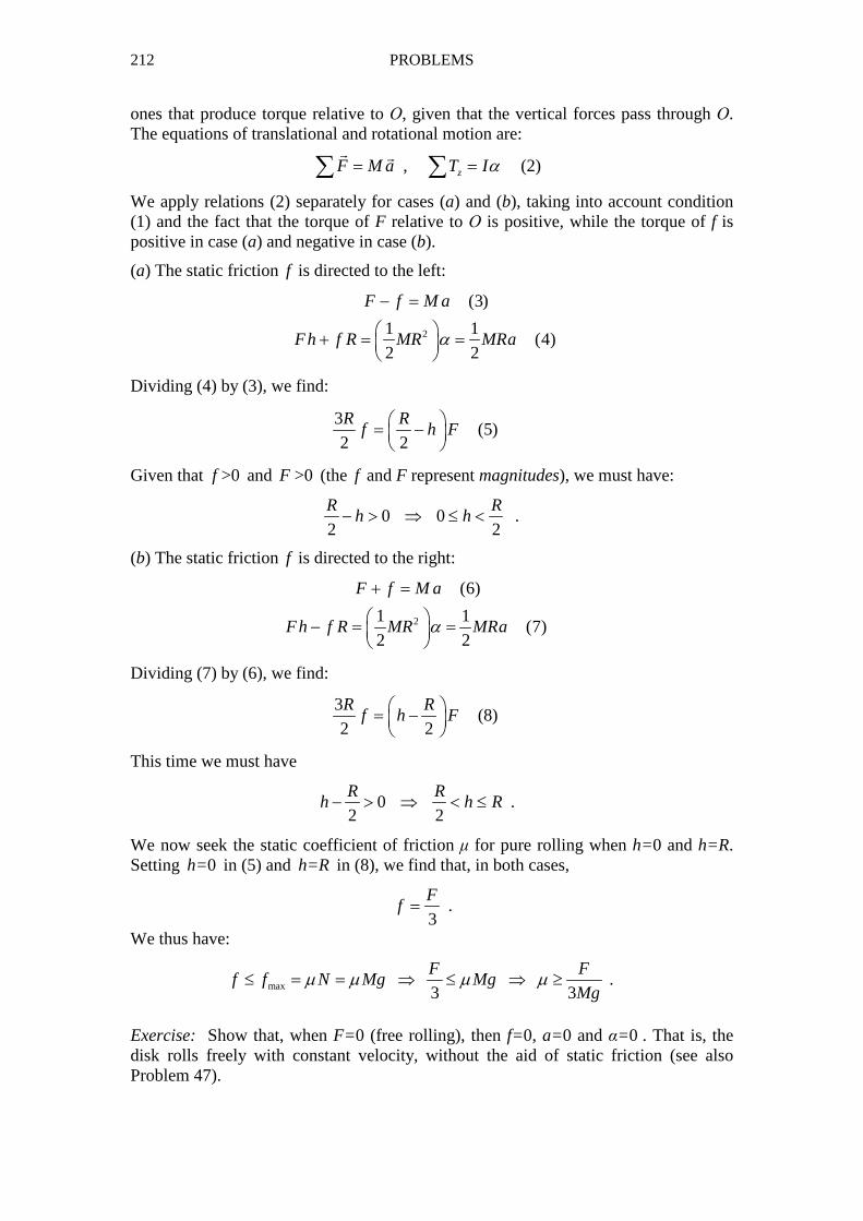
212 PROBLEMS
ones that produce torque relative to Ο, given that the vertical forces pass through Ο. The equations of translational and rotational motion are:
, zF M a T Iα= =∑ ∑� �
(2)
We apply relations (2) separately for cases (a) and (b), taking into account condition (1) and the fact that the torque of F relative to Ο is positive, while the torque of f is positive in case (a) and negative in case (b).
(a) The static friction f is directed to the left:
2
(3)
1 1(4)
2 2
F f M a
Fh f R MR MRaα
− =
+ = =
Dividing (4) by (3), we find:
3
(5)2 2
R Rf h F = −
Given that f >0 and F >0 (the f and F represent magnitudes), we must have:
0 02 2
R Rh h− > ⇒ ≤ < .
(b) The static friction f is directed to the right:
2
(6)
1 1(7)
2 2
F f M a
Fh f R MR MRaα
+ =
− = =
Dividing (7) by (6), we find:
3
(8)2 2
R Rf h F = −
This time we must have
02 2
R Rh h R− > ⇒ < ≤ .
We now seek the static coefficient of friction µ for pure rolling when h=0 and h=R. Setting h=0 in (5) and h=R in (8), we find that, in both cases,
3
Ff = .
We thus have:
max 3 3
F Ff f N Mg Mg
Mgµ µ µ µ≤ = = ⇒ ≤ ⇒ ≥ .
Exercise: Show that, when F=0 (free rolling), then f=0, a=0 and α=0 . That is, the disk rolls freely with constant velocity, without the aid of static friction (see also Problem 47).

PROBLEMS 213
49. A disk of radius R and mass Μ has a string wound around it. A mass m is at-tached to the end of the string, as shown in figure 1. As the string is unwound, the mass m moves downward while the disk rolls without slipping on the horizontal sur-face. Find the accelerations a1 and a2 of the disk and the mass, the tension F of the string, and the static friction f (magnitude and direction) at the point of contact Ο. (The moment of inertia of the disk is I = ½ MR2.)
i
mM
O
RC
P F
2a
⋅1a
Fig. Problem 49 (1)
Solution: Since we don’t yet know the direction of the friction f, we will arbitrarily assume that it is to the right. If we find a negative magnitude for f at the end, our as-sumption will prove to be incorrect. The acceleration a1 of the disk is, by definition, the acceleration of its center of mass C relative to the horizontal surface, or, equiva-lently, relative to the point of contact Ο: a1= aC,O . The acceleration a2 of m with re-spect to the horizontal surface (directed downward) is equal in magnitude to the ac-celeration of the highest point P of the disk, relative to the surface (or, relative to Ο): a2= aP,O . In Sec. 7.10 we showed that aP,O= 2aC,O . Therefore,
a2 = 2a1 (1) We set a1 = a , a2 = 2a .
If α is the angular acceleration of the disk relative to C, the condition for pure rolling demands that a1 = a = Rα (2)
M
Cα
Mg
N
R
R
F
f
am
F
mg
2a+
+
+
Fig. Problem 49 (2) In figure 2 we draw the forces on each body separately. The positive directions for translation and rotation are as indicated in the figure (the moving z-axis of rotation of the disk is normal to the page and directed into it). The total force on Μ is (F+f ) (since N=Mg), while that on m is (mg−F ). The Mg and Ν do not produce torque rela-tive to C, since they both pass through C. Thus, the total torque on Μ relative to C is
214 PROBLEMS
( )zT F R f R F f R= − = −∑
(notice that the torque of F is positive, while that of f is negative). We write the equa-tions of translational motion for m and for Μ, as well as the equation of rotational mo-tion for Μ :
mg – F = m(2a) = 2ma (3)
F + f = Ma (4)
(2)
21 1( )
2 2F f R I MR F f M aα α − = = ⇒ − =
(5)
Dividing (4) by (5) ⇒ F = 3f (6)
From (4) and (6) ⇒ f = 4
Ma (7)
From (6) and (7) ⇒ F = 3
4
Ma (8)
From (3) and (8) ⇒ a = a1 = 4
8 3
mg
m M+ (9) √
From (1) and (9) ⇒ a2 = 8
8 3
mg
m M+ (10) √
From (7), (8) and (9) ⇒ f = 8 3
M mg
m M+ , F =
3
8 3
M mg
m M+ (11) √
We notice that f > 0; thus, the arbitrarily chosen direction for f was correct. Equations (9), (10) and (11) constitute the solution to the problem.
50. A student is sitting on a stool that can rotate about a frictionless vertical axis. The student is holding, with both arms extended, a pair of dumbbells, each of mass m, while the stool is rotating with an initial angular velocity ω1 . The student now pulls the dumbbells closer to his body, so that their initial distance R1 from the axis of rota-tion decreases to R2 . (a) Find the new angular velocity ω2 of the stool. Assume, ap-proximately, that the moment of inertia of the system “stool + student” (without the dumbbells) remains unchanged, equal to Ι0 . (b) Compare the initial with the final ki-netic energy of the system (with the dumbbells). Solution: Consider the system “stool + student + dumbbells”. Its initial and its final moment of inertia is, respectively,
I1 = I0 + mR12 + mR1
2 = I0 + 2mR12 ,
I2 = I0 + 2mR22 .
The angular momentum of the system, relative to any point of the z-axis of rotation (which is a principal axis), is directed parallel to the axis. Its initial and its final value is, respectively,
PROBLEMS 215
L1 = I1 1ω = (I0 + 2mR12) 1ω ,
L2 = I2 2ω = (I0 + 2mR22) 2ω .
The external forces on the system are the weights of the bodies and the reaction of the floor on the stool. Since all of these forces are in the vertical direction, none of them produces torque about the axis of rotation. Hence, ΣTz=0, so that the angular momen-tum of the system is constant:
1 2 1 1 2 2L L I Iω ω= ⇒ = ⇒
2
0 112 1 12
2 0 2
2
2
I mRI
I I mRω ω ω
+= =
+ .
Note that ω2>ω1 , given that R1>R2 .
The initial and the final kinetic energy of the system is, respectively, Ek,1= ½ I1ω12
and Ek,2= ½ I2 ω22 . Thus,
2 2
2,2 2 2 1 1
,1 1 1 1 2 2
1k
k
E I I I I
E I I I I
ω
ω
= = = >
.
That is, Ek,2 > Ek,1 . Given that the external forces produce no work (why?) the in-crease of total kinetic energy is due to the work of the internal forces (specifically, the work done by the student in pulling the dumbbells closer to his body).

216 PROBLEMS
PROBLEMS FOR CHAP. 8 51. A homogeneous sphere of density ρ1 is let to sink inside a vessel containing a liq-uid of density ρ (where ρ<ρ1), as seen in the figure. The height of the free surface of the liquid above the bottom of the vessel is h. (a) Find the time t1 it will take the sphere to reach the bottom. (b) If a second sphere of density ρ2>ρ1 is let to sink simul-taneously with the first sphere, which sphere will reach the bottom first?
O
y ρh
1w
1a ˆ yu
1A
Fig. Problem 51
Solution: (a) Call m1 , V1 , w1 the mass, the volume and the weight, respectively, of the first sphere. Then, m1=ρ1V1 and
1 1 1 1w m g gVρ= = .
The buoyant force on the sphere is equal to the weight of the displaced liquid:
1 1A gVρ= .
The total force on the sphere is
1 1 1 1 1 1 1 1 1ˆ ˆ ˆ ˆ( ) ( ) ( )y y y yF w A w u A u w A u gV uρ ρ= + = + − = − = −�� �
.
By Newton’s law,
1 1 1 1 1 1 1 1ˆ ˆ( )y yF m a m a u V a uρ= = =� �
.
Hence,
1 1 1 1 1 11
( ) 1V a gV a gρ
ρ ρ ρρ
= − ⇒ = −
(1)
Since a1= constant, the motion of the sphere is uniformly accelerated. Therefore,
20 0 1
1
2y y v t a t= + +
where, in our case, y0=0, v0=0, y=h and t=t1 . Thus,
21 1 1
1
1 2
2
hh a t t
a= ⇒ = , where a1 is given by (1).
(b) Similarly, for the second sphere we have:
22
2ht
a= where 2
2
1a gρρ
= −
.
Given that ρ1< ρ2 , we see that a1< a2 , so that t1>t2 . That is, the denser sphere ρ2 will reach the bottom first, regardless of the dimensions of the two spheres !
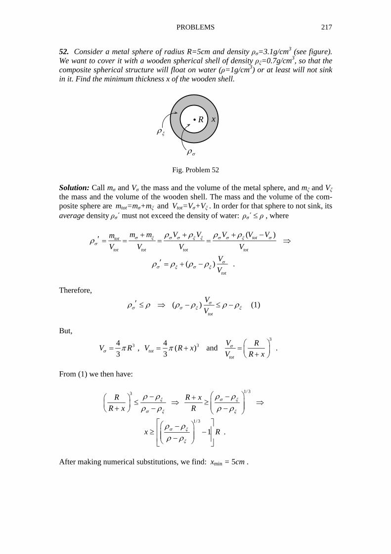
PROBLEMS 217
52. Consider a metal sphere of radius R=5cm and density ρσ=3.1g/cm3 (see figure). We want to cover it with a wooden spherical shell of density ρξ=0.7g/cm3, so that the composite spherical structure will float on water (ρ=1g/cm3) or at least will not sink in it. Find the minimum thickness x of the wooden shell.
i R x
σρ
ξρi
Fig. Problem 52 Solution: Call mσ and Vσ the mass and the volume of the metal sphere, and mξ and Vξ the mass and the volume of the wooden shell. The mass and the volume of the com-posite sphere are mtot=mσ+mξ and Vtot=Vσ+Vξ . In order for that sphere to not sink, its average density ρσ΄ must not exceed the density of water: ρσ΄ ≤ ρ , where
( )
( ) .
tottot
tot tot tot tot
tot
m m V V V V Vm
V V V V
V
V
σ ξ σ σ ξ ξ σ σ ξ σσ
σσ ξ σ ξ
ρ ρ ρ ρρ
ρ ρ ρ ρ
+ + + −′ = = = = ⇒
′ = + −
Therefore,
( )tot
V
Vσ
σ σ ξ ξρ ρ ρ ρ ρ ρ′ ≤ ⇒ − ≤ − (1)
But,
3 34 4, ( )
3 3totV R V R xσ π π= = + and 3
.tot
V R
V R xσ = +
From (1) we then have:
1/ 33
1/3
1 .
R R x
R x R
x R
ξ σ ξ
σ ξ ξ
σ ξ
ξ
ρ ρ ρ ρ
ρ ρ ρ ρ
ρ ρ
ρ ρ
− −+ ≤ ⇒ ≥ ⇒ + − −
− ≥ − −
After making numerical substitutions, we find: xmin = 5cm .
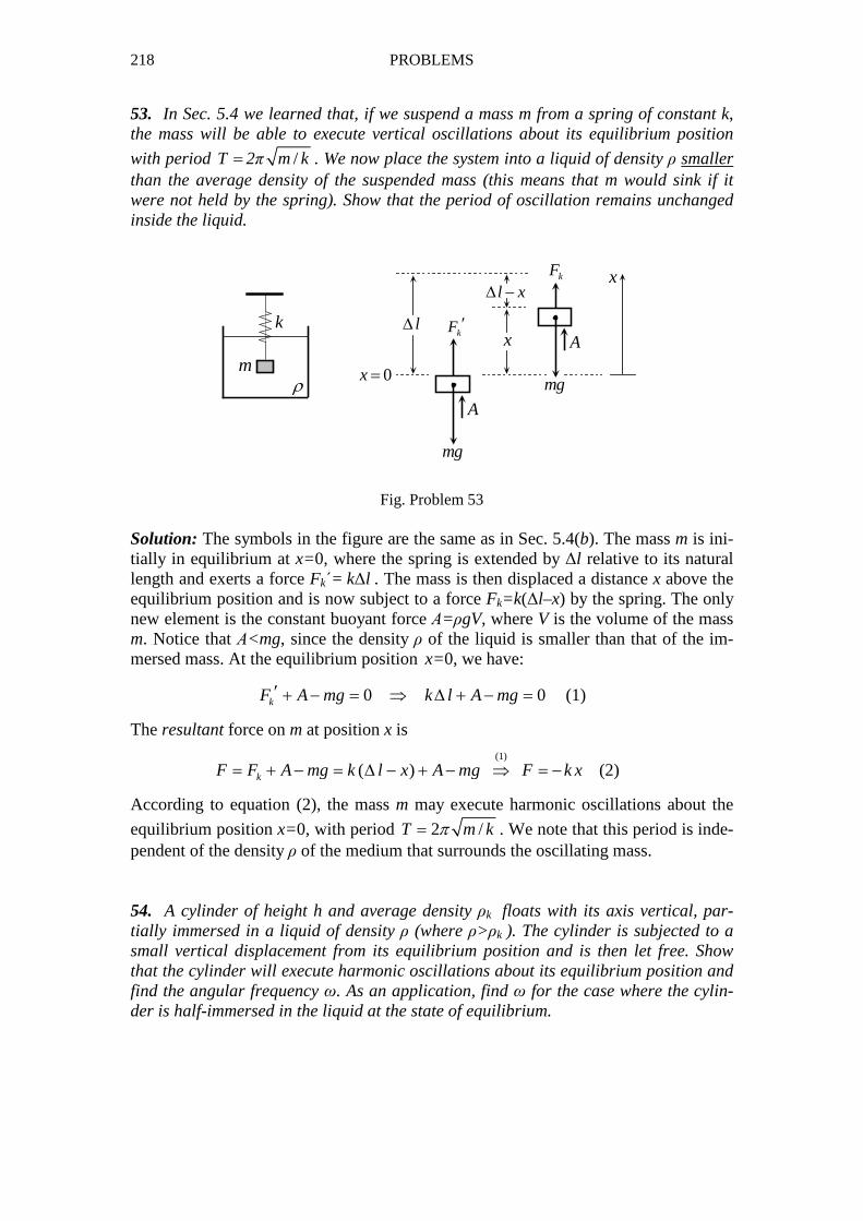
218 PROBLEMS
53. In Sec. 5.4 we learned that, if we suspend a mass m from a spring of constant k, the mass will be able to execute vertical oscillations about its equilibrium position
with period T = 2π /m k . We now place the system into a liquid of density ρ smaller than the average density of the suspended mass (this means that m would sink if it were not held by the spring). Show that the period of oscillation remains unchanged inside the liquid.
Fig. Problem 53 Solution: The symbols in the figure are the same as in Sec. 5.4(b). The mass m is ini-tially in equilibrium at x=0, where the spring is extended by ∆l relative to its natural length and exerts a force Fk΄= k∆l . The mass is then displaced a distance x above the equilibrium position and is now subject to a force Fk=k(∆l–x) by the spring. The only new element is the constant buoyant force Α=ρgV, where V is the volume of the mass m. Notice that Α<mg, since the density ρ of the liquid is smaller than that of the im-mersed mass. At the equilibrium position x=0, we have:
0 0kF A mg k l A mg′ + − = ⇒ ∆ + − = (1)
The resultant force on m at position x is
(1)
( )kF F A mg k l x A mg F k x= + − = ∆ − + − ⇒ = − (2)
According to equation (2), the mass m may execute harmonic oscillations about the
equilibrium position x=0, with period 2 /T m kπ= . We note that this period is inde-pendent of the density ρ of the medium that surrounds the oscillating mass. 54. A cylinder of height h and average density ρk floats with its axis vertical, par-tially immersed in a liquid of density ρ (where ρ>ρk ). The cylinder is subjected to a small vertical displacement from its equilibrium position and is then let free. Show that the cylinder will execute harmonic oscillations about its equilibrium position and find the angular frequency ω. As an application, find ω for the case where the cylin-der is half-immersed in the liquid at the state of equilibrium.
m
k
ρ
mg
A
kF ′
mg
A
kF
0x=
l∆x
l x∆ −x
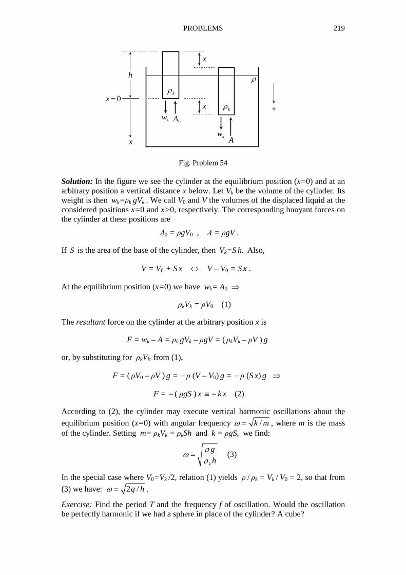
PROBLEMS 219
kρ
kw0A
kρ
kwA
ρ
+
x
x
x
0x=
h
Fig. Problem 54 Solution: In the figure we see the cylinder at the equilibrium position (x=0) and at an arbitrary position a vertical distance x below. Let Vk be the volume of the cylinder. Its weight is then wk=ρk gVk . We call V0 and V the volumes of the displaced liquid at the considered positions x=0 and x>0, respectively. The corresponding buoyant forces on the cylinder at these positions are
Α0 = ρgV0 , Α = ρgV .
If S is the area of the base of the cylinder, then Vk=S h. Also,
V = V0 + S x ⇔ V – V0 = S x .
At the equilibrium position (x=0) we have wk= A0 ⇒
ρkVk = ρV0 (1)
The resultant force on the cylinder at the arbitrary position x is
F = wk – A = ρk gVk – ρgV = ( ρkVk – ρV ) g
or, by substituting for ρkVk from (1),
F = ( ρV0 – ρV ) g = − ρ (V – V0) g = − ρ (S x) g ⇒
F = − ( ρgS ) x ≡ − k x (2)
According to (2), the cylinder may execute vertical harmonic oscillations about the
equilibrium position (x=0) with angular frequency /k mω = , where m is the mass of the cylinder. Setting m= ρkVk = ρkSh and k = ρgS, we find:
k
g
h
ρω
ρ= (3)
In the special case where V0=Vk /2, relation (1) yields ρ / ρk = Vk / V0 = 2, so that from
(3) we have: 2 /g hω = .
Exercise: Find the period Τ and the frequency f of oscillation. Would the oscillation be perfectly harmonic if we had a sphere in place of the cylinder? A cube?
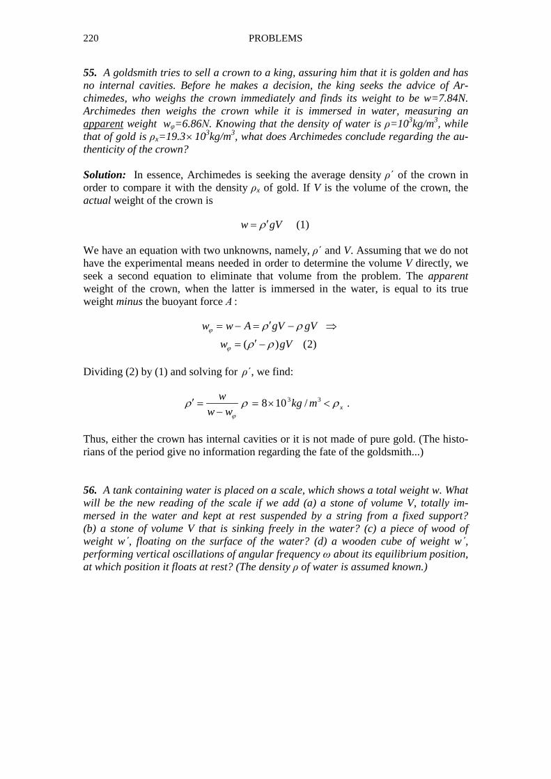
220 PROBLEMS
55. A goldsmith tries to sell a crown to a king, assuring him that it is golden and has no internal cavities. Before he makes a decision, the king seeks the advice of Ar-chimedes, who weighs the crown immediately and finds its weight to be w=7.84N. Archimedes then weighs the crown while it is immersed in water, measuring an apparent weight wφ=6.86Ν. Knowing that the density of water is ρ=103kg/m3, while that of gold is ρx=19.3×10³kg/m3, what does Archimedes conclude regarding the au-thenticity of the crown? Solution: In essence, Archimedes is seeking the average density ρ΄ of the crown in order to compare it with the density ρx of gold. If V is the volume of the crown, the actual weight of the crown is
w gVρ ′= (1)
We have an equation with two unknowns, namely, ρ΄ and V. Assuming that we do not have the experimental means needed in order to determine the volume V directly, we seek a second equation to eliminate that volume from the problem. The apparent weight of the crown, when the latter is immersed in the water, is equal to its true weight minus the buoyant force Α :
( ) (2)
w w A gV gV
w gV
ϕ
ϕ
ρ ρ
ρ ρ
′= − = − ⇒
′= −
Dividing (2) by (1) and solving for ρ΄, we find:
3 38 10 / .x
wkg m
w wϕ
ρ ρ ρ′ = = × <−
Thus, either the crown has internal cavities or it is not made of pure gold. (The histo-rians of the period give no information regarding the fate of the goldsmith...) 56. A tank containing water is placed on a scale, which shows a total weight w. What will be the new reading of the scale if we add (a) a stone of volume V, totally im-mersed in the water and kept at rest suspended by a string from a fixed support? (b) a stone of volume V that is sinking freely in the water? (c) a piece of wood of weight w, floating on the surface of the water? (d) a wooden cube of weight w, performing vertical oscillations of angular frequency ω about its equilibrium position, at which position it floats at rest? (The density ρ of water is assumed known.)
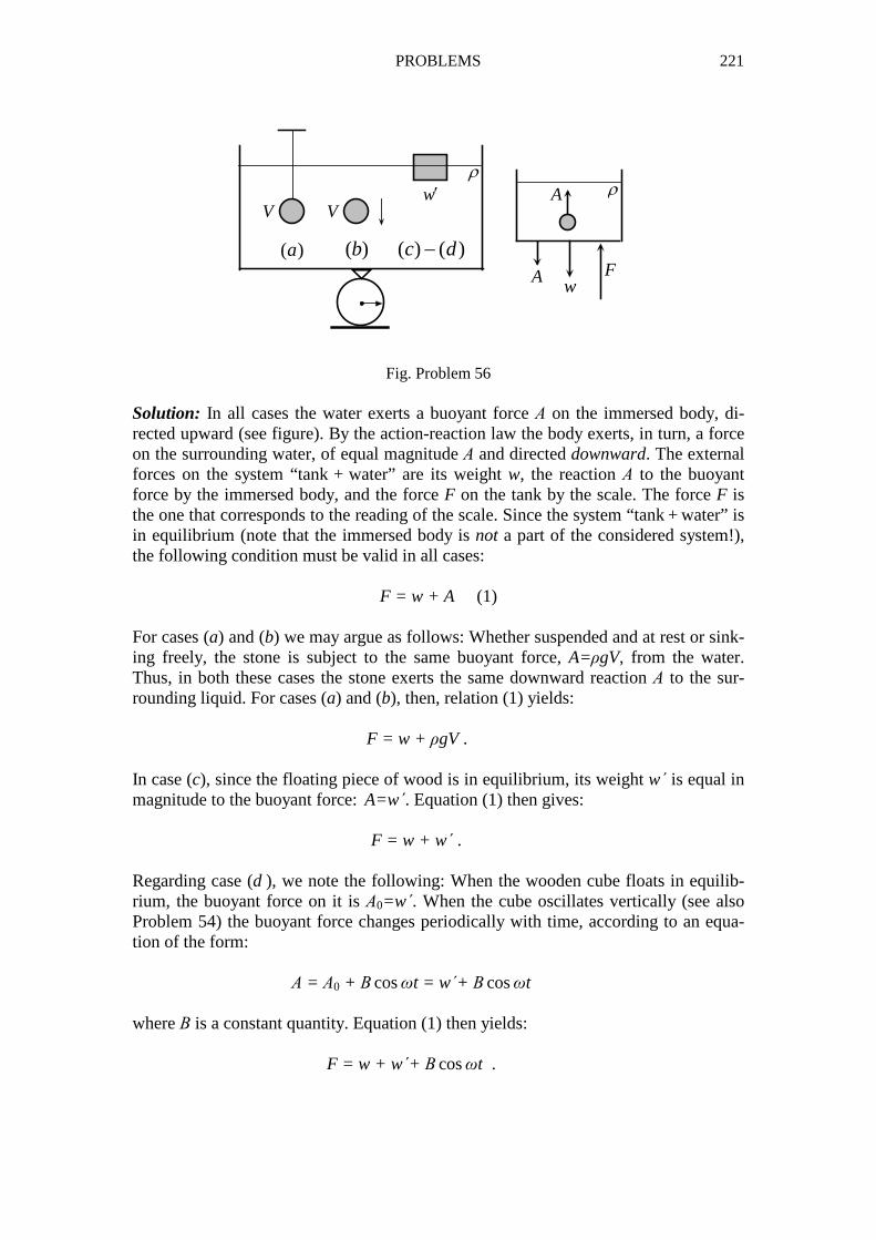
PROBLEMS 221
A
A wF
ρ
( )a ( )b ( ) ( )c d−
V Vw′
ρ
Fig. Problem 56 Solution: In all cases the water exerts a buoyant force Α on the immersed body, di-rected upward (see figure). By the action-reaction law the body exerts, in turn, a force on the surrounding water, of equal magnitude Α and directed downward. The external forces on the system “tank + water” are its weight w, the reaction Α to the buoyant force by the immersed body, and the force F on the tank by the scale. The force F is the one that corresponds to the reading of the scale. Since the system “tank + water” is in equilibrium (note that the immersed body is not a part of the considered system!), the following condition must be valid in all cases: F = w + A (1) For cases (a) and (b) we may argue as follows: Whether suspended and at rest or sink-ing freely, the stone is subject to the same buoyant force, A=ρgV, from the water. Thus, in both these cases the stone exerts the same downward reaction Α to the sur-rounding liquid. For cases (a) and (b), then, relation (1) yields: F = w + ρgV . In case (c), since the floating piece of wood is in equilibrium, its weight w΄ is equal in magnitude to the buoyant force: A=w΄. Equation (1) then gives: F = w + w΄ . Regarding case (d ), we note the following: When the wooden cube floats in equilib-rium, the buoyant force on it is Α0=w΄. When the cube oscillates vertically (see also Problem 54) the buoyant force changes periodically with time, according to an equa-tion of the form: Α = Α0 + Β cos ωt = w΄+ Β cos ωt where Β is a constant quantity. Equation (1) then yields: F = w + w΄+ Β cos ωt .
222 PROBLEMS
57. A container of uniform cross-sectional area Α is filled with a liquid of density ρ. On the wall of the container, at a vertical distance h below the free surface of the liq-uid, we open a hole of area a, where a<<A . Find the initial velocity of outflow of the liquid from the hole, as well as the volume flow rate of the initial outflow. (The liquid is considered ideal.)
1
2
0P
0P
h
1y
2yv
y
0y =
Fig. Problem 57 Solution: As soon as we open the hole, a tube of flow (a few streamlines of which are shown in the figure) is formed, extending from the free surface of the liquid (cross-section Α2=Α) to the hole (cross-section Α1= a). The hydrostatic pressure at both these cross-sections is equal to the atmospheric pressure: P1=P2=P0 . We call v1= v and v2 the flow velocities at the considered cross-sections, and we call y1, y2 the heights at which these cross-sections are located above an arbitrary horizontal reference level. By the equation of continuity,
11 1 2 2 2 1 2
2
0A a
A v A v v v v vA A
= ⇒ = = ⇒ ≃ (1)
since a<<A , by assumption, so that a /A≃ 0. By Bernoulli’s equation,
(1)2 2
1 1 1 2 2 2
2 20 1 0 2 2 1
1 1
2 21
2 ( )2
2 .
P v g y P v g y
P v g y P g y v g y y
v gh
ρ ρ ρ ρ
ρ ρ ρ
+ + = + + ⇒
+ + = + ⇒ = − ⇒
=
Notice that the velocity of initial outflow is independent of the density ρ of the liquid. The volume flow rate is
2 .a v a ghΠ = =
Exercise: Do the problem again, this time assuming that the area a of the hole is not negligible compared to the cross-sectional area Α of the container. Show that the exact value of the initial velocity of outflow is
1/ 2
2
2
1
ghv
aA
= −
( 2gh≃ when 1a
A<< ) .
PROBLEMS 223
58. A horizontal tube of cross-sectional area Α1 narrows to a coaxial tube of cross-section Α2 (Α2<Α1), as shown in the figure. A vertical tube is attached at position 1 of the wider section, while another vertical tube is attached at position 2 of the narrower section. Water flows inside this horizontal coaxial system of tubes, while inside the vertical tubes the (static) water rises to corresponding heights h1 and h2 . (a) In which of the two vertical tubes does the water rise higher? (b) Find the volume flow rate of the horizontal flow, given the Α1 , Α2 , h1 , h2 .
12
0P 0P
1h2h
1A 2A1v 2v
Fig. Problem 58 Solution: We assume that the water columns in the two vertical tubes are measured, approximately, from the axis of the horizontal system of tubes. Since the water is static inside the vertical tubes, we can use the fundamental equation of Hydrostatics to find the pressures at the cross-sections 1 and 2:
1 0 1 2 0 2,P P gh P P ghρ ρ= + = + (1)
where ρ is the density of water and Ρ0 is the atmospheric pressure. Now, as we showed in Sec. 8.13, in horizontal flow the pressure is greater where the cross-section of the tube of flow is greater. Given that Α1>Α2 , we must have Ρ1>Ρ2 . It thus follows from relations (1) that h1>h2 . That is, the water rises to a greater height at the vertical tube attached to the wider section of the coaxial system.
By the equation of continuity,
11 1 2 2 2 1
2
AA v A v v v
A= ⇒ = (2)
where v1, v2 are the flow velocities at the two cross-sections. By Bernoulli’s equation for horizontal flow,
2 21 1 2 2
1 1
2 2P v P vρ ρ+ = + (3)
Substituting (1) and (2) into (3), and solving for v1, we find:
1/ 2
1 21 2 2 2
1 2
2 ( )g h hv A
A A
−=
− .
The flow rate is
1/ 2
1 21 1 1 2 2 2
1 2
2 ( )g h hA v A A
A A
−Π = =
− .
224 PROBLEMS
59. At the bottom of a very large tank we open a hole of area a=1cm2 (which is con-sidered negligible compared to the cross-sectional area of the tank). We now place the tank under a faucet from which water flows at a volume rate of Π=140cm3/s. At what height h will the free surface of the water rise in the tank? (g=980cm/s2)
ρ
h
a
v
Π
Fig. Problem 59 Solution: There is an incoming flow of water in the tank, of constant volume flow rate Π (see figure). At the same time there is an outgoing flow through the hole. The level of the water in the tank is initially rising, since the outgoing flow rate, equal to a.v (where v is the velocity of outflow from the hole) is less than the incoming flow rate Π. The water level will stop rising as soon as the two flow rates become equal:
avΠ = (1)
Now, the hole is at a vertical distance h below the free surface of water in the tank. As we showed in Problem 57, the outflow velocity for a given (albeit now variable) h is
2v gh= (2)
(it makes no difference that this time the hole is at the bottom, rather than on the wall, of the tank). From (1) and (2) we have:
2
210 .
2h cm
ga
Π= =
60. Water is running from a faucet of cross-sectional area A, at a constant volume flow rate Π. Find the cross-sectional area of the column of water at a vertical dis-tance h below the faucet, as a function of Π, A and h.
y
0y =
0y
y
h
A
a
0P
0P
0v
v
Fig. Problem 60
PROBLEMS 225
Solution: Let a be the cross-sectional area of the column of water at distance h below the faucet; let v be the flow velocity at that cross-section; and let y be the height at which the cross-section a is located above an arbitrary horizontal reference level (see figure). At the “mouth” of the faucet (cross-section Α) the corresponding quantities are v0 and y0. The pressure at both cross-sections Α and a is equal to the atmospheric pressure Ρ0 . We apply the laws of Hydrodynamics at these cross-sections, assuming that all conditions of ideal flow are satisfied.
By the equation of continuity, 0Av a vΠ = = (1)
By Bernoulli’s equation,
2 2
0 0 0 0
2 2 20 0 0
1 1
2 2
2 ( ) 2 (2)
P v g y P v g y
v v g y y v v gh
ρ ρ ρ ρ+ + = + + ⇒
= + − ⇒ = +
From (1) ⇒
0vA
Π= (3) and a
v
Π= (4)
where the flow rate Π is assumed known. By substituting (2) and (3) into (4), we fi-nally have:
2
2
a
ghA
Π=
Π +
.
226
MATHEMATICAL SUPPLEMENT
1. Differential of a Function Consider a function y= f (x) . Let ∆x be an arbitrary change of the independent vari-able, from its initial value x to x+∆x . The corresponding change of y is
( ) ( )y f x x f x∆ = + ∆ − .
Note that ∆y is a function of two independent variables, x and ∆x. The derivative of f at a point x is defined as
0 0
( ) ( )( ) lim lim
x x
f x x f x yf ΄ x
x x∆ → ∆ →
+ ∆ − ∆= =
∆ ∆ (1)
It follows from (1) that a function ( , )x xε ∆ must exist such that
( ) ( , )y
f ΄ x x xx
ε∆
= + ∆∆
where 0
lim ( , ) 0x
x xε∆ →
∆ = (2)
Thus, y∆ = f (x) x∆ + ( , )x x xε ∆ ∆ (3) The product f ΄(x)∆x is linear (i.e., of the first degree) in ∆x, while the product
( , )x x xε ∆ ∆ must only contain terms that are at least of the second degree in ∆x (that is, it may not contain a constant or a linear term). We write, symbolically,
2( , ) ( )x x x O xε ∆ ∆ ≡ ∆ where ∆ x2 ≡ (∆ x)2 ( ≠∆ (x
2) ! ) .
Equation (3) is then written as
y∆ = f (x) x∆ + 2( )O x∆ (4) We notice that ∆y is the sum of a linear and a higher-order term in ∆x. Furthermore, the derivative of f at x is the coefficient of ∆x in the linear term. Example: Let y = f (x) = x 3
. Then,
∆y = f (x+∆x) – f (x) = (x+∆x) 3 – x 3 = 3x 2 ∆x + (3x∆x 2 + ∆x 3) ,
by which we have that f ΄ (x) = 3x 2 and 2( )O x∆ = 3x∆x 2 + ∆x 3 .
The linear term in (4), which is a function of x and ∆x, is called the differential of the function y = f (x) and is denoted dy : ( )dy df x= = f (x) x∆ (5)
227
Equation (4) is then written:
y dy∆ = + 2( )O x∆ (6)
If ∆x is infinitesimal (|∆x|<< 1) we can make the approximation 2( ) 0O x∆ ≃ . Hence,
y dy∆ ≃ = f ΄ (x) x∆ for infinitesimal ∆ x (7) Careful, however: for finite (i.e., non-infinitesimal) ∆x, the difference ∆y and the dif-ferential dy are, in general, separate quantities! An exception to the above general remark occurs in the case of linear functions. Let y = f (x) = ax+b . Then, ∆y = f (x+∆x) – f (x) = [a(x+∆x)+b] – (ax+b) = a∆x
and dy = f ΄ (x) x∆ = (ax+b)΄ ∆x = a∆x = ∆y . That is, for linear functions (and only for such functions) the differential dy is the same as the difference ∆y, even if these quantities assume finite values. This means that, for these functions, 2( ) 0O x∆ = . Let us see a few applications of the definition (5) of the differential:
For 1( ) ( ) ( )a a a af x x d x x x ax x−′= ⇒ = ∆ = ∆ ;
for ( ) ( ) ( )x x x xf x e d e e x e x′= ⇒ = ∆ = ∆ ;
for 1
( ) ln (ln ) (ln )f x x d x x x xx
′= ⇒ = ∆ = ∆ .
In particular, for f (x)=x , we have: ( ) 1dx x x x′= ∆ = ⋅ ∆ ⇒ x dx∆ = (8) in accordance with the remark made earlier regarding linear functions. Equation (5) may thus be rewritten in a more symmetric form: ( )dy df x= = f (x)dx (9) By dividing the above relation by dx, we can express the derivative as follows:
f ΄ (x)( )dy df x
dx dx= = (10)
In words: The derivative of a function is equal to the differential of the function di-vided by the differential (or, the change) of the independent variable.

228
2. Differential Operators We introduce a notation that proves to be important in higher mathematics:
( )
( )df x d
f xdx dx
≡ (11)
Note that this notation tries to “mimic” the properties of ordinary multiplication of numbers:
α β α
βγ γ⋅
= ⋅
except that the expression d
dx is not a number! The symbol
d
dx is called a differential
operator and, when placed in front of a function f (x), it instructs us to take the de-rivative of f (x). We thus write:
f ΄ (x)( )
( )df x d
f xdx dx
= = (12)
Relation (12) contains three different notations for the derivative of a function. Higher-order derivatives can also be expressed in terms of differential operators. Thus, the second derivative of y= f (x) is written:
f ΄΄ (x)2 2
2
( )( ) ( ) ( )
d df x d d d df x f x f x
dx dx dx dx dx dx = = = =
or
f ΄΄ (x)2 2
2 2
( )d f x d y
dx dx= = (13)
Exercise: Verify the following properties of the differential:
1. [ ( ) ( )] ( ) ( )d f x g x df x dg x± = ±
2. [ ( ) ( )] ( ) ( ) ( ) ( )d f x g x f x dg x g x df x= +
3. [ ( )] ( )d c f x cdf x= (c=const.)
4. 2
( ) ( ) ( ) ( ) ( )
( ) [ ( )]
f x g x df x f x dg xd
g x g x
−=
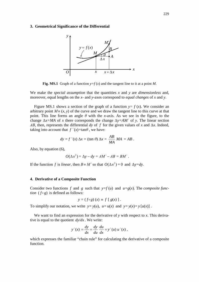
229
3. Geometrical Significance of the Differential
i
i
ii
Ox
y
θMA
B
x x x+∆
x∆
M ′( )y f x=
Fig. MS.1 Graph of a function y=f (x) and the tangent line to it at a point M. We make the special assumption that the quantities x and y are dimensionless and, moreover, equal lengths on the x- and y-axes correspond to equal changes of x and y. Figure MS.1 shows a section of the graph of a function y= f (x). We consider an arbitrary point Μ≡ (x, y) of the curve and we draw the tangent line to this curve at that point. This line forms an angle θ with the x-axis. As we see in the figure, to the change ∆x=MA of x there corresponds the change ∆y=AM΄ of y. The linear section ΑΒ, then, represents the differential dy of f for the given values of x and ∆x. Indeed, taking into account that f ΄ (x)= tanθ , we have:
dy = f (x) ∆x = (tan θ) ∆x = AB
MAMA
= AB .
Also, by equation (6),
2( )O x∆ = ∆y – dy = ΑΜ΄ – ΑΒ = ΒΜ΄ .
If the function f is linear, then Β≡Μ΄ so that 2( )O x∆ = 0 and ∆y=dy. 4. Derivative of a Composite Function Consider two functions f and g such that y=f (u) and u=g(x). The composite func-tion ( f �g) is defined as follows:
y = ( f �g) (x) ≡ f [ g(x) ] .
To simplify our notation, we write y= y(u), u= u(x) and y= y(x)= y [u(x)] . We want to find an expression for the derivative of y with respect to x. This deriva-tive is equal to the quotient dy/dx . We write:
y΄ (x) dy dy du
dx du dx= = = y΄ (u) u΄ (x) ,
which expresses the familiar “chain rule” for calculating the derivative of a composite function.
230
5. Differential Equations In the case of an algebraic equation the solution is a set of numbers (real or complex). On the other hand, the solution of a differential equation is a set of functions. A first-order differential equation is an algebraic relation involving the derivative of an un-known function as well as, possibly, the function itself. An equation of this kind ad-mits an infinite number of solutions. In order to specify a particular solution, in addi-tion to the differential equation one must also be provided with an initial condition. Let us see a few examples:
1. Determine the function y=y(x) that satisfies the differential equation
y΄ = 2xe (14)
as well as the initial condition
y = 1 for x = 0 (15) Solution: Equation (14) is written:
2 2x xdye dy e dx
dx= ⇒ = (16)
We can proceed in two ways:
(a) Take the indefinite integral of (16) in order to find the general solution of (14):
2 2 21 2 2 1
1 1( )
2 2x x xdy e dx y C e C y e C C= ⇒ + = + ⇒ = + −∫ ∫
or, since the constants C1, C2 are arbitrary,
21
2xy e C= + (17)
Note that the general solution (17) represents an infinite set of functions correspond-ing to the various values of the arbitrary constant C. By applying the initial condition (15) to (17), we can determine the value of the constant C :
01 11
2 2e C C= + ⇒ = .
By (17) we then find the particular solution
21( 1)
2xy e= + .
(b) Take the definite integrals of the two sides of (16), putting as lower limits the corresponding values of y and x given by the initial condition (15) (as upper limits simply place the variables y and x):
2 2 2 0 2
1 00
1 1 1 11 ( 1)
2 2 2 2
xy x x x x xdy e dx y e e e y e = ⇒ − = = − ⇒ = + ∫ ∫ .
Note that this second way is the shortest if we are only interested in finding a particu-lar solution of the differential equation.
231
2. Solve the differential equation y΄ = 5y , with the initial condition: y=3 for x=0. Solution:
[ ] 33 0
5
5 5 5 ln 5
ln 5 3 .3
y x y
x
dy dy dyy dx dx y x
dx y y
yx y e
= ⇒ = ⇒ = ⇒ = ⇒
= ⇒ =
∫ ∫
3. Solve the equation y΄ =2
2 1x + , with the initial condition: y=0 for x=0.
Solution:
0 0
0
2 22
2 1 2 1 2 1
12 ln(2 1) ln(2 1) .
2
y x
x
dy dx dxdy dy
dx x x x
y x x
= ⇒ = ⇒ = ⇒+ + +
= + = +
∫ ∫
4. Solve the equation y΄ = 2 xy, with the initial condition: y=5 for x=1. Solution:
2
5 1
2 1
2 2 2
ln 1 5 .5
y x
x
dy dy dyx y xdx xdx
dx y y
yx y e −
= ⇒ = ⇒ = ⇒
= − ⇒ =
∫ ∫
Exercise: Find the particular solutions of the differential equations of Examples (2)–(4), this time by first finding the general solutions of the equations and then ap-plying the initial conditions to determine the values of the corresponding constants, as in Example 1(a).
232
BASIC INTEGRALS
dx x C= +∫
1
( 1)1
aa x
x dx C aa
+
= + ≠ −+∫
ln | |dx
x Cx
= +∫
x xe dx e C= +∫
2
2
cos sin
sin cos
tancos
cotsin
xdx x C
x dx x C
dxx C
x
dxx C
x
= +
= − +
= +
= − +
∫
∫
∫
∫
2arcsin
1
dxx C
x= +
−∫
2arctan
1
dxx C
x= +
+∫
2
1 1ln
1 2 1
dx xC
x x
−= +
− +∫
( )2
2ln 1
1
dxx x C
x= + ± +
±∫
233
INDEX Accelerated motion, 17 Acceleration, 12, 16, 21 Acceleration of gravity, 34, 178 Amplitude (SHM), 64 Angular acceleration, 25, 98 Angular acceleration vector, 111 Angular frequency (SHM), 64 Angular momentum, 41, 81, 101 Angular velocity, 25 Angular velocity vector, 111 Archimedes’ principle, 132-134 Atmosphere (unit), 128 Atmospheric pressure, 128, 158 Atwood’s machine, 203 Average density, 135 Ballistic pendulum, 196 Bar (unit), 128 Bernoulli’s equation, 140-142, 159, 160 Buoyant force (buoyancy), 133 Cartesian coordinates, 6 Center of buoyancy, 133 Center of curvature, 23 Center of gravity, 93, 148, 149 Center of mass, 76, 79, 92, 149, 150-153 Center-of-mass frame (C-frame), 81, 82 Center of parallel forces, 147 Central force, 46, 82, 151 Centripetal acceleration, 21 Centripetal force, 40 Circular motion, 24, 43 Closed line integral, 55, 56 Coefficients of friction, 36 Collision, 87 Communicating vessels, 129-131 Completely inelastic collision, 88, 195 Concurrent forces, 145 Conical pendulum, 175 Conservation of angular momentum, 45, 82, 88, 109-113 Conservation of mechanical energy, 56, 85 Conservation of momentum, 31, 79, 87 Conservative force, 53, 54, 85 Coulomb force, 47, 61 Couple, 113, 145 Curvilinear motion, 15 Density, 93 Differential equation, 48, 230, 231 Differential equation of SHM, 74
234
Differential of a function, 226 Differential operator, 228 Displacement, 12 Distance between points, 6, 7 Elastic collision, 88, 89, 90 Elastic force, 60, 68 Equation for rotational motion (rigid body), 104 Equation for translational motion (rigid body), 103 Equation of continuity, 139, 140 Equilibrium, 34, 113 Equilibrium position (SHM), 67 Escape velocity, 188 External force, 76, 78 External potential energy, 85, 116 Floating body, 135-137 Flow velocity, 137 Fluid flow, 137 Force, 30 Force field, 46, 48, 53 Force of gravity, 34, 58 Frame of reference, 26 Free fall, 173 Free particle, 29 Frequency (SHM), 66 Frequency (uniform circular motion), 26 Friction, 35, 36, 62, 119 Fundamental equation of Hydrostatics, 127, 142 Gauge pressure, 131 Gyroscope, 121 Gyroscopic compass, 121 Gyroscopic motion, 120, 121 Harmonic oscillation, 64 Hertz (unit), 26, 66 Horizontal flow, 142, 143 Hydraulic lever, 132 Hydrostatic pressure, 124 Ideal flow, 137 Ideal fluid, 123 Inelastic collision, 88 Inertia, 30 Inertial frame of reference, 29 Inertial observer, 29 Initial condition, 12, 48, 230 Internal force, 32, 76 Internal potential energy, 85 Isolated system, 31, 79 Joule (unit), 51 Kinetic energy, 52, 83, 88 Kinetic energy of rotation, 115, 116 Kinetic energy of translation, 115, 116
235
Kinetic friction, 36, 62 Law of Action and Reaction (Newton’s Third Law), 32 Law of Inertia (Newton’s First Law), 29 Line integral, 50 Linear density, 94 Linear momentum, 30 Mass, 30 Mass-spring system, 68-72 Metacenter, 137 Moment of inertia, 98, 102, 106, 154 Momentum, 30, 77 Neutral equilibrium, 136 Newton (unit), 33 Newton’s Law of Gravity, 34, 178 Newton’s Second Law, 30, 78 Non-conservative force, 54, 57, 62, 85, 86 Non-inertial frame of reference, 173 Open-tube manometer, 131 Parallel-axis theorem, 107 Parallel forces, 145-148 Pascal (unit), 128 Pascal’s principle, 127, 131, 132 Pendulum, 72, 74 Period (SHM), 65 Period (uniform circular motion), 26 Periodic motion, 64 Phase (SHM), 64 Plane of rolling, 117 Plastic collision, 88, 89, 195 Polar coordinates, 6 Position vector, 5, 6 Potential energy, 54, 85 Power, 51 Principal axis, 110, 155-157 Projectile motion, 14, 163 Pure rolling, 117, 118 Radius of curvature, 23 Rectilinear motion, 11, 24 Reduced mass, 194 Relative acceleration, 27 Relative motion, 26 Relative velocity, 26 Restoring couple, 136 Restoring force, 69, 73 Resultant (total) force, 33, 144 Retarded motion, 17 Rigid body, 92 Rolling body, 117-120 Rolling without slipping, 117 Rotational equilibrium, 113
236
Scalar (dot) product, 7, 8 Simple harmonic motion (SHM), 64 Speed, 11, 16, 17 Spinning top, 121 Stable equilibrium, 136 Static friction, 35, 36, 119, 120 Steiner’s theorem, 107 Streamline, 138 Tangential and normal acceleration, 21 Tangential and normal force, 40 Torque, 43 Torque of a couple, 114 Torr (unit), 128 Total angular momentum, 81, 150 Total external force, 78 Total external torque, 81, 151 Total kinetic energy, 84, 152 Total mechanical energy, 56, 85, 116 Total momentum, 77 Translational equilibrium, 113 Tube of flow, 138 Uniform circular motion, 25, 40, 64, 65 Uniform motion, 17, 24, 49 Uniform rectilinear motion, 13, 24 Uniformly accelerated motion, 13 Unit vector, 1 Unstable equilibrium, 136 Vector, 1 Vector (cross) product, 8, 9 Velocity, 11, 15, 20 Volume flow rate (volume flux), 140 Watt (unit), 51 Weight, 34, 92 Work, 49 Work-energy theorem, 52, 53, 83, 84