See discussions, stats, and author profiles for this publication at: https://www.researchgate.net/publication/349104699

Introduction to Mathematical Logic, Edition 2021

Book · February 2021

CITATIONS

0READ

1

2 authors, including:

Some of the authors of this publication are also working on these related projects:

Truth Demystified View project

Philosophy of Modeling in 1870s: a Tribute to Hans Vaihinger View project

Karlis Podnieks

University of Latvia

75 PUBLICATIONS   273 CITATIONS   

SEE PROFILE

All content following this page was uploaded by Karlis Podnieks on 07 February 2021.

The user has requested enhancement of the downloaded file.

1

Version released: February 7, 2021

This edition is dedicated to the memory of Professor Elliott Mendelson, 1931-2020

Introduction to Mathematical Logic

Textbook for students

Edition 2021

by Vilnis Detlovs, Dr. math.,and Karlis Podnieks, Dr. math.

University of Latvia

This work is licensed under a Creative Commons License and iscopyrighted © 2000-2021 by us, Vilnis Detlovs and Karlis Podnieks.

Sections 1, 2, 3 of this book represent an extended translation of the corresponding chapters of the book: V. Detlovs, Elements of Mathematical Logic, Riga, University of Latvia, 1964, 252 pp. (in Latvian). With kind permission of Dr. Detlovs.

Vilnis Detlovs, 1923-2007. Memorial Page

This textbook contains links to:Wikipedia, the free encyclopedia;

MacTutor History of Mathematics archive of the University of St Andrews;MathWorld of Wolfram Research.

2

Table of ContentsReferences..........................................................................................................31. Introduction. What Is Logic, Really?.............................................................4

1.1. Total Formalization is Possible!..............................................................41.2. Predicate Languages.............................................................................111.3. Axioms of Logic: Minimal System, Constructive System and Classical System..........................................................................................................271.4. The Flavor of Proving Directly.............................................................401.5. Deduction Theorems.............................................................................44

2. Propositional Logic......................................................................................522.1. Proving Formulas Containing Implication only...................................522.2. Proving Formulas Containing Conjunction..........................................532.3. Proving Formulas Containing Disjunction...........................................562.4. Formulas Containing Negation – Minimal Logic.................................582.5. Formulas Containing Negation – Constructive Logic..........................632.6. Formulas Containing Negation – Classical Logic................................652.7. Constructive Embedding: Glivenko's Theorem....................................692.8. Axiom Independence. Using Computers in Mathematical Proofs........71

3. Predicate Logic.............................................................................................873.1. Proving Formulas Containing Quantifiers and Implication only..........873.2. Formulas Containing Negations and a Single Quantifier.....................913.3. Proving Formulas Containing Conjunction and Disjunction..............1003.4. Replacement Theorems.......................................................................1013.5. Constructive Embedding.....................................................................107

4. Completeness Theorems (Model Theory)..................................................1164.1. Interpretations and models..................................................................1164.2. Completeness of Classical Propositional Logic..................................1324.3. Classical Predicate Logic − Gödel's Completeness Theorem.............1434.4. Constructive Propositional Logic – Kripke Semantics.......................164

5. Normal Forms.............................................................................................1845.1. Negation Normal Form.......................................................................1845.2. Conjunctive and Disjunctive Normal Forms......................................1865.3. Prenex Normal Form..........................................................................1905.4. Skolem Normal Form.........................................................................1985.5. Clause Form........................................................................................202

6. Tableaux Method........................................................................................2096.1. Tableaux Method for Propositional Formulas....................................2106.2. Tableaux Method for Pure Predicate Formulas..................................217

7. Resolution Method.....................................................................................2277.1. Resolution Method for Propositional Formulas..................................2307.2. Resolution Method for Predicate Formulas........................................235

3

8. Miscellaneous.............................................................................................2478.1. Negation as Contradiction or Absurdity.............................................2478.2. Herbrand's Theorem............................................................................254

ReferencesDetlovs V. [1964] Elements of Mathematical Logic, University of Latvia, 1964, 252 pp. (in Latvian).

Hilbert D., Bernays P. [1934] Grundlagen der Mathematik. Vol. I, Berlin, 1934, 471 pp. (Russian translation available)

Kleene S.C. [1952] Introduction to Metamathematics. Van Nostrand, 1952 (Russian translation available)

Kleene S.C. [1967] Mathematical Logic. John Wiley & Sons, 1967 (Russian translation available)

Mendelson E. [1997] Introduction to Mathematical Logic. Fourth Edition. International Thomson Publishing, 1997, 440 pp. (Russian translation available)

Podnieks K. [1997] What is Mathematics: Gödel's Theorem and Around. 1997-2015 (see ResearchGate for English and Russian online versions).

4

1. Introduction. What Is Logic, Really?

Attention! In this book,

predicate language is used as a synonym of first order language,

formal theory – as a synonym of formal system, deductive system,

predicate logic – as a synonym of first order logic without equality.

constructive logic – as a synonym of intuitionistic logic,

algorithmically solvable – as a synonym of recursively solvable,

algorithmically enumerable – as a synonym of recursively enumerable.

1.1. Total Formalization is Possible!

What is logic? Of course, logic is “about reasoning”. Parts of our knowledgemay be inter-dependent, so, one part may be derived from some other ones. Atrivial example:

All fathers are male persons.

No person can be male and female simultaneously.

Miranda is a female person.

Hence, Miranda is not a father.

Of course, we knew the latter “fact” in advance. But imagine, we are trying toteach this kind of reasoning to a computer. A computer may know in advanceonly that part of our knowledge that is stored in its knowledge base. But, it isimpossible to store all of our knowledge. Thus, we must avoid storing of theknowledge that is easily derivable from the one already stored. For example, ifthe first three of the above propositions have been already stored, then we neednot to store the fourth one – it can be derived by reasoning:

Assume, Miranda is a father. Then Miranda is a male person. But Miranda is a female person.Hence, Miranda is male and female simultaneously. This is impossible. Hence, Miranda is nota father.

Therefore, we must implement on our computer not only the knowledge base,but also the necessary means of reasoning (an advanced kind of queryprocessing).

Hence, today, we have a very fundamental reason to formulate our knowledge

5

and means of reasoning explicitly: only in this way we can transmit theknowledge and the ability of reasoning to computers.

Of course, explicit reasoning started long before computers – probably, in the6th century BC when Greeks proved the first mathematical theorems. Let usconsider one of them:

Theorem. There are more prime numbers than any prescribed amount. (In modern terms:there are infinitely many prime numbers.)

Proof (modern notation is used). Assume the contrary, that p1 , ... , pk is the complete list

of all primes, and consider the number N=p1⋅...⋅pk+1 . We know that such N is

divisible by none of p1 , ... , pk . But we know also that any (natural) number is divisible bya prime. So, N must be divisible by a prime that does not belong to the alleged “complete”list. Q.E.D.

Here, the statement of Theorem is derived from other statements that “weknow”. How do we know them? Either we or other people have proved thesestatements earlier – by deriving them from some other statements, or, theywere forced to adopt them without proof, for example, as “obvious” ones.Indeed, asking for proofs over and again indefinitely long time is hopeless. Atsome moment, such a process must be stopped – by a decision to adopt someof the statements without proof, as “axioms”.

Additional stimulus to explicit reasoning was a contradiction found ingeometrical reasoning. The early Pythagoreans arrived at an implicit beliefthat any two line segments must possess a common measure. Namely (inmodern terms), if x and y are lengths of two line segments, then there exists a(usually, smaller) segment z such that x=pz ; y=qz , where p, q are somenatural numbers. Of course, if z is the maximum common measure, then p, qpossess no common divisors. Now, let us try to find the common measure of xand y being the side and the diagonal of a square. By Pythagorean Theorem:x2+x2=2 x2= y2 . But there is a maximum z such that

x=pz ; y=qz ;2 p2 z2=q2 z2 ;2 p2=q2 .

Hence, q is even: q=2r ;q2=4 r2; p2=2 r2 . Thus, p is even as well, but weknow that p and q do not possess common divisors. We have arrived at acontradiction! According to a legend, this caused a serious conflict amongPythagoreans. The solution was found by abandoning the belief in theuniversal existence of common measures, and by re-building the geometryaccordingly.

Note. Of course, in modern terms, Pythagoreans discovered that √2 is anirrational number, i.e., that there are no natural numbers p, q such that

√2= qp

(or, 2 p2=q2 , see above).

6

How far can people proceed with explication? Can any implicit knowledge(intuition) be converted into an explicit knowledge represented as a list ofaxioms? Can any sophisticated human skills of reasoning be converted into anexplicit list of rules of inference? Is this really possible?

It took more than 2000 years to develop the necessary methods. The processended in 1870s and subsequent decades – in the work of Georg Cantor,Gottlob Frege, Charles S. Peirce, Bertrand Russell, David Hilbert, of theircolleagues and followers. Today, the logical techniques developed by thesepeople allow for an axiomatic reconstruction of any theory that is based on astable system of principles (in particular, of any mathematical theory).

Total axiomatic reconstruction is called formalization. The results of suchreconstruction are called formal theories (the terms “formal systems” and“deductive systems” also are used) emphasizing that in these theories no stepof reasoning can be done without a reference to an exactly formulated list ofaxioms and rules of inference. Even the most "self-evident" logical principles(like as, "if A implies B, and B implies C, then A implies C") must be eitherformulated in the list of axioms and rules explicitly, or must be derived from it.

Modern students can think of formal theories as knowledge bases. In thesebases, knowledge is stored in the form of propositions, also called axioms.The simplest kind of axioms are facts representing data of the usual databases,for example, personal data of people, such as “Miranda is a female person”.The second kind of axioms are rules representing data constraints, such as“All fathers are male persons”. Knowledge bases are equipped with queryprocessing software. However, the situation with query processing is heremore complicated than in the case of the usual databases. For example,imagine, we would wish to ask “Is Miranda a father?” This would mean, infact, asking the question: which of the propositions, “Miranda is a father” or“Miranda is not a father” follows from the axioms stored in the knowledgebase?

The first distinctive feature of a formal theory (or, knowledge base) must be aprecisely defined ("formal") language used to express its propositions."Precisely defined" means here that there is an algorithm allowing todetermine, is a given character string a correct proposition, or not.(Algorithms are mechanically applicable procedures that do not refer toimplicit knowledge or human skills. Algorithms can be implemented ascomputer programs. For more details, see Algorithm in Wikipedia)

The second distinctive feature of a formal theory must be a precisely defined("formal") notion of proof. Each proof proves some proposition, that is called(after being proved) a theorem. Thus, theorems form a subset of propositions.

What could mean here “precisely defined”? Curiously enough, the most

7

general definition is very simple, and it does not mention neither axioms, norrules of inference: precisely defined notion of proof means that there is analgorithm allowing to determine, is a given text a correct proof, or not.

Neither "self-evident" axioms, nor "plausible" rules of inference are distinctivefeatures of the "formality". Speaking strictly, "self-evident" is synonymous to"accepted without argument". Hence, axioms and/or rules of inference may be"good, or bad", "true, or false", and so may be the theorems obtained by meansof them. The only definitely verifiable thing is here the fact that some theoremhas been, indeed, proved by using some definite set of axioms, and by meansof some definite set of inference rules. And this fact must be verifiable bymeans of an algorithm – by a procedure that can be implemented on acomputer.

Thus, a theory T is called a formal theory if and only if there are twoalgorithms:

a) an algorithm allowing to verify, is a given character string a correctproposition of T, or not;

b) an algorithm allowing to verify, is a given text a correct proofaccording to the principles of T, or not.

If somebody is going to publish a "mathematical text" calling it "proof of atheorem in theory T", then we must be able to verify whether the text inquestion is really a correct proof according to the standards of provingaccepted in theory T. Thus, in a formal theory, the standards of reasoningshould be defined precisely enough to implement verification of proofs on acomputer. But note that we are discussing here verification of ready proofs,and not the much more difficult problem – is some proposition provable in Tor not, see below.

Axioms and rules of inference represent the most popular of the possibletechniques of formalization (see Exercise 1.1.7 below).

Chess game as a formal “theory”

As an unpractical example of a formal theory let us consider the game ofchess, let us call this "theory" CHESS. Let 's define as propositions of CHESSall the possible positions – i.e., allocations of some of the pieces (kingsincluded) on a chessboard – plus the flag: "white to move" or "black to move".Thus, the set of all the possible positions represents the language of CHESS.The only axiom of CHESS is the initial position (“white to move” included),and the rules of inference – the well-known rules of the game. Rules define“proof steps” – they allow correct passing from some propositions of CHESSto some other ones. Starting with the axiom and iterating moves allowed bythe rules we obtain theorems of CHESS. Thus, theorems of CHESS aredefined as all the possible positions (i.e., propositions of CHESS) that can be

8

obtained from the initial position (the axiom of CHESS) by moving piecesaccording to the rules of the game (i.e., by using the inference rules ofCHESS). Note that here, correct silly moves are considered as correct “proofsteps”.

Exercise 1.1.1 (optional). Could you provide an unprovable proposition of CHESS? Tryproving that your proposition is unprovable, indeed, i.e., that your position cannot be obtainedfrom the initial position by moving pieces according to the rules of the game.

Note. By the way, as you see it now, and will see later again: in logic,“negative” proving, i.e., proving that something cannot be proved, may be amore complicated task than “positive” proving.

Why could CHESS be called a formal theory? When somebody offers a"mathematical text" P as a proof of a theorem A in CHESS, this means that Pis a record of some chess-game stopped in the position A. Checking thecorrectness of such "proofs" is a boring, but an easy task. The rules of thegame are formulated precisely enough – we could write a computer programthat will execute the task.

Exercise 1.1.2 (optional). Try estimating the size of this program in some programminglanguage.

Another toy example

Our second example of a formal theory is only a bit more serious. It wasproposed by Paul Lorenzen, so let us call this theory Lo. Propositions of Loare all the possible (non-empty) "words" made of letters a, b, for example: a,b, aa, aba, baab. Thus, the set of all these "words" represents the language ofLo. The only axiom of Lo is the word a, and Lo has two rules of inference:

X├ Xb; X├ aXa.

This means that (in Lo) from a proposition X we can infer immediately thepropositions Xb and aXa. For example, the proposition aababb is a theorem ofLo:

a ├ ab ├ aaba ├ aabab ├ aababbrule1 rule2 rule1 rule1

This fact is expressed usually as Lo├ aababb ( "Lo proves aababb", ├ being a"fallen T").

Exercise 1.1.3. a) Verify that Lo is a formal theory. (Hint: describe analgorithm allowing to determine, is a sequence of propositions of Lo a correctproof, or not.)

b) (P. Lorenzen) Verify the following property of theorems of Lo: for any X, if Lo├ X, then Lo├ aaX.

9

General properties of formal theories

One of the most important properties of formal theories is given in thefollowing

Exercise 1.1.4. Show that the set of all theorems of a formal theory isalgorithmically enumerable, i.e., show that, for any formal theory T, one canbuild an algorithm AT that generates and prints out on an endless paper tape all

theorems of this theory (and nothing else). (Hint: we will call T a formaltheory if and only if we can present an algorithm for checking texts as correctproofs via principles of reasoning of T. Thus, assume, you have 4 functions:GenerateFirstText() – returns Text, GenerateNextText() – returns Text,IsCorrectProof(Text) – returns true or false, ExtractTheorem(Text) – returnsText, and you must implement the functions GenerateFirstTheorem() – returnsText, GenerateNextTheorem() – returns Text).

Unfortunately, such generating algorithms cannot solve the problem thatthe mathematicians are mainly interested in: is a given proposition Aprovable in T or not? Indeed, when, executing the algorithm AT, we see our

proposition A printed out, this means that A is provable in T. Still, in general,until that moment, we cannot know in advance whether A will be printed outsome time later or it will not be printed at all.

Note. According to the official terminology, algorithmically enumerable sets are called"recursively enumerable sets", in some texts – also "listable sets".

Exercise 1.1.5. a) Describe an algorithm determining whether a proposition ofLo is a theorem or not.

b) (optional) Could you imagine such an algorithm for CHESS? Of course,you could, yet... Thus you see that even, having a relatively simple algorithmfor checking the correctness of proofs, the problem of determining provabilitycan be a very complicated one.

T is called a solvable theory (more precisely – algorithmically solvabletheory) if and only if there is an algorithm allowing to check whether someproposition is provable by using the principles of T or not.

In the Exercise 1.1.5(a) you proved that Lo is a solvable theory. Still, in theExercise 1.1.5(b) you established that it is hard to state whether CHESS is a"feasibly solvable" theory or not. Determining the provability ofpropositions is a much more complicated task than checking thecorrectness of ready proofs. It can be proved that most mathematicaltheories are unsolvable, the elementary (first order) arithmetic of naturalnumbers included (see, for example, Mendelson [1997], or Podnieks [1997],Section 6.3). There is no algorithm allowing to determine, is some arithmeticalproposition provable from the axioms of arithmetic, or not.

10

Note. According to the official terminology, algorithmically solvable sets are called "recursivesets".

Normally, formal theories contain the negation symbol not. In such theories,solving of the problem stated in a proposition A means proving either A, orproving notA ("disproving A", "refuting A"). We could try to solve the problemby using the enumeration algorithm of the Exercise 1.1.4: let us wait until A ornotA is printed. In general, we have four possibilities here:

a) A will be printed, but notA will not (then the problem A has a positivesolution);

b) notA will be printed, but A will not (then the problem A has a negativesolution);

c) A and notA will be printed both;

d) neither A, nor notA will be printed.

In the case c), by using principles of T, some proposition and its negation canbe proved simultaneously, i.e., T is an inconsistent theory. This means thatthe principles of T must be re-examined (to determine the cause ofinconsistency) and corrected.

In the case d) we may be waiting forever, yet nothing interesting will happen:by using the principles of T one can neither prove nor disprove the propositionA, and for this reason such a theory is called an incomplete theory. Thefamous Incompleteness Theorem proved by Kurt Gödel in 1930 says that mostmathematical theories are either inconsistent or incomplete (seeMendelson [1997] or Podnieks [1997], Section 6.1).

Exercise 1.1.6. Show that any (simultaneously) consistent and completeformal theory is solvable. (Hint: use the algorithm of the Exercise 1.1.4, i.e.,assume that you have the functions GenerateFirstTheorem() − returns Text,GenerateNextTheorem() − returns Text, and implement the functionIsProvable(Text) that returns true or false. Where the consistency andcompleteness come in here?)

Exercise 1.1.7 (optional). a) Verify that "fully axiomatic theories" are formal theories in thesense of the above general definition. (Hint: assume, that you have the following functions:GenerateFirstText() − returns Text, GenerateNextText() − returns Text, IsPropositon(Text) −returns true or false, IsAxiom(Proposition) − returns true or false, there is a finite list ofinference rule names: {R1, ..., Rn}, function Apply(RuleName, ListOfPropositions) − returns

Proposition or false, and you must implement the functions IsCorrectProof(ListOfPropositions) − returns true or false, ExtractTheorem(Proof) − returns Proposition).

b) (for smart students) What, if, instead of {R1, ..., Rn}, we would have an infinite list of

inference rules, i.e., functions GenerateFirstRule(), GenerateNextRule() returning RuleName?

11

1.2. Predicate Languages

History

Aristotle (384-322 BC) – in a sense, the "first logician", "... was not primarily a mathematicianbut made important contributions by systematizing deductive logic." (according to MacTutorHistory of Mathematics archive).

Gottlob Frege: "In 1879 Frege published his first major work Begriffsschrift, eine derarithmetischen nachgebildete Formelsprache des reinen Denkens. ... In this work Fregepresented for the first time what we would recognise today as a logical system with negation,implication, universal quantification, essentially the idea of truth tables etc." (according toMacTutor History of Mathematics archive).

Hilary Putnam. Peirce the Logician. Historia Mathematica, Vol. 9, 1982, pp. 290-301 (anonline excerpt available, published by John F. Sowa).

Imagine, we are trying to build a knowledge base (or, a formal theory) bymaking explicit some piece of our (until now – mainly implicit) knowledge.How should we proceed?

We have an informal vision of some domain consisting of “objects”. Whenspeaking about it, we are uttering various propositions, and some of thesepropositions we regard as “true” statements about the domain. Thus, our firstformalization task must be defining of some formal language, allowing to putall our propositions about the domain in a uniform and precise way.

After this, we can start considering propositions that we are regarding as“true” statements about the domain. There may be an infinity of suchstatements, hence, we can't store into knowledge base all of them, so we mustorganize them somehow. Some minimum of the statements we will declare asaxioms, and store in the knowledge base. The other ones we will try to derivefrom the axioms by using some precisely defined rules of inference.

Formulation of axioms (in knowledge bases they are called facts and rules)and rules of inference (i.e., logic) is an absolutely necessary next step, if wewish to transmit our knowledge to computers. In advance, computers “do notknow” even the most trivial things about the human society, such as “personscannot be parents of themselves”. Or, about natural numbers: we must submitto our computer, for example, x+0=x as an axiom, if we wish it to learnproving of mathematical theorems.

In mathematics and computer science, the most common approach to the firstphase of formalization is using of the so-called predicate languages, firstintroduced by G. Frege and C. S. Peirce.

(In most textbooks, they are called first order languages, however, see below the warningabout second order languages.)

12

Usually, we are taught to analyze the sentence "John loves Britney" as follows:John – subject, loves – predicate, Britney – object. The approach of predicatelanguages is different: instead of "John loves Britney", let us write

loves(John, Britney),

where loves(x, y) is a two-argument predicate, and John, and Britney areobjects. By the way, following this principle literally, we should write =(x, y)instead of x=y.

Another example: in a predicate language, to say “All people are mortal”, wewill write: “for all x, if x is a person, then x is mortal”, or,

∀ x( person(x)→mortal(x)) .

This approach – reducing of human language sentences to variables,constants, functions, predicates and quantifiers, appears to be extremelyflexible, and it is much more uniform when compared to the variety ofconstructs used in natural human languages. A unified approach is much easierto use for communication with computers.

Yet another example: "Britney works for BMI as a programmer". In a predicate language, wemust introduce a 3-argument predicate "x works for y as z", or works(x, y, z). Then, we mayput the above fact as: works(Britney, BMI, Programmer).

Note. Representing data in the form of predicates was the main idea of Edgar F. Codd when heintroduced relational databases (“SQL databases”) in 1970. Database tables representpredicates.

Language primitives

The informal vision behind the notion of predicate languages is centered onthe so-called "domain" – a non-empty collection of "objects", their"properties" and the "relations" between them, that we wish to describe byusing the language. This vision serves as a guide in defining the formallanguage, and further – when selecting axioms and rules of inference.

Object variables

The first kind of language elements we will need are object variables(sometimes called also individual variables, or simply, variables). We need anunlimited number of them):

x, y, z, x1, y1, z1,...

The above-mentioned "domain" is the intended “range” of all these variables.

Examples. 1) Building a language that should describe the "domain of people", we must start by introducing "variables for people": x denotes an arbitrary person.

2) Building the language of the so-called first order arithmetic, we are thinking about "all

13

natural numbers" as the range of variables: 0, 1, 2, 3, 4, …: x denotes here an arbitrary naturalnumber.

3) Building the language of set theory, we think about "all sets" as the range of variables: x denotes an arbitrary set.

“Domain of people” represented as a UML class diagram

Note. Since our screens and printers allow only a limited number of pixels perinch, in principle, we should generate variable names by using a finite set ofcharacters. This can be achieved, for example, by using a single letter x:

x, xx, xxx, xxxx, xxxxx,...

Object constants

The next possibility we may wish to have in our language are the so-calledobject constants (sometimes called individual constants, constant letters, orsimply, constants) – names or symbols denoting some specific "objects" of our"domain".

Examples. 1) In our "language about people" we may introduce constants identifyingparticular people: John, Britney etc.

2) In the language of first order arithmetic, we may wish to introduce two constants – 0 and 1to denote "zero" and "one" – two natural numbers having specific properties.

3) In the language of set theory, we could introduce a constant denoting the empty set, butthere is a way to do without it as well (for details, Podnieks [1997], Section 2.3).

Function constants

In some languages we may need also the so-called function constants(sometimes called function letters) – names or symbols denoting specificfunctions, i.e., mappings between "objects" of our "domain", or operations on

14

these objects.

Examples. 1) In our "language about people" we will not use function constants.

2) In the language of first order arithmetic, we introduce two function constants "+" and "*"denoting the usual addition and multiplication of natural numbers, i.e., the two-argumentfunctions x+y and x*y.

3) In the language of set theory, we could introduce function constants denoting setintersections x∩y , unions x∪ y , set differences x – y , power sets P (x) etc.,but there is a way to do without these symbols as well (for details, Podnieks [1997], Section2.3).

In mathematics, normally, we are writing f(x, y) to denote the value of thefunction f for the argument values x, y. This (the so-called "prefix" notation) isa uniform way suitable for functions having any number of arguments: f(x),g(x, y), h(x, y, z) etc. In our everyday mathematical practice some of the two-argument functions (in fact, operations) are represented by using the moreconvenient "infix" notation (x+y, x*y instead of the uniform +(x, y), *(x, y),etc.).

Note. In a sense, object constants can be viewed as a special case of functionconstants – an object constant is a “zero-argument function”.

Predicate constants

The last (but the most important!) kind of primitives we need in our languageare the so-called predicate constants (sometimes called predicate letters) –names or symbols denoting specific properties (of) or relations between"objects" of our "domain".

Note. Using "predicate" as the unifying term for "property" and "relation" mayseem somewhat unusual. But some kind of such unifying term is necessary.Properties are, in fact, unary (i.e., one-argument) "predicates", for example, "xis red". Relations are, two- or more-argument "predicates", for example, "x isbetter than y", or "x sends y to z".

Examples. 1) In our "language about people" we will use the following predicate constants(see the class diagram above):

Male(x) − means "x is a male person";

Female(x) − means "x is a female person";

Mother(x, y) − means "x is mother of y";

Father(x, y) − means "x is father of y";

Married(x, y) − means "x and y are married";

x=y − means "x and y are the same person".

The first two constants represent, in fact, "properties" (or, "classes") of our objects. The other4 constants represent "relations" between our objects. The term "predicate" is used to include

15

both versions. We do not introduce Person(x) as a separate predicate because our domainsconsists of persons only.

2) It may seem strange to non-mathematicians, yet the most popular relation of objects used inmost mathematical theories, is equality (or identity). Still, this is not strange formathematicians. We can select an object x in our "domain" by using a very specificcombination of properties and relations of it, and then – select another object y – by using adifferent combination. And after this (sometimes it may take many years to do) we prove thatx=y, i.e., that these two different combinations of properties and relations are possessed by asingle object. Many of the discoveries in mathematics could be reduced to this form.

In the language of first order arithmetic, equality "=" is the only necessary predicate constant.Other "basic" relations must be reduced to equality. For example, the relation x<y for naturalnumbers x, y can be reduced to equality by using the addition function and the formula

z(x+z+1=y).∃z(x+z+1=y).

3) In the language of set theory a specific predicate constant "in" denotes the set membershiprelation: x∈ y means "x is a member of y". The equality predicate x=y also is used – itmeans "the sets x and y possess the same members".

The uniform way of representation suitable for predicates having any numberof arguments is again the "prefix" notation: p(x), q(x, y), r(x, y, z) etc. In thereal mathematical practice, some of the two-argument predicates arerepresented by using the "infix" notation (for example, x=y instead of theuniform =(x, y), etc.).

Zero-argument predicate constants? In an interpretation (see Section 4.1 below), each suchpredicate must become either "true", or "false". Hence, paradoxically, zero-argument predicateconstants would behave like as "propositional variables" – they represent assertions that do notpossess a meaning, but possess a "truth value".

Summary of language primitives

Thus, the specification of a predicate language includes the followingprimitives:

1) A countable set of object variable names.

2) An empty, finite, or countable set of object constants.

3) An empty, finite, or countable set of function constants. To each functionconstant a fixed argument number must be assigned.

4) A finite, or countable set of predicate constants. To each predicate constant afixed argument number must be assigned.

Different sets of primitives yield different predicate languages.

Examples. 1) Our "language about people" is based on: a) object variables x, y, z, ...; b) objectconstants: John, Britney, ...; c) function constants: none; d) predicate constants: Male(x),Female(x), Mother(x, y), Father(x, y), Married(x, y), x=y.

2) The language of first order arithmetic is based on: a) object variables x, y, z, ...; b) objectconstants: 0, 1; c) function constants: x+y, x*y; d) predicate constant: x=y.

16

3) The language of set theory is based on: a) object variables x, y, z, ...; b) object constants:none; c) function constants: none; d) predicate constants: x∈ y , x= y .

The remaining part of the language definition is common for all predicatelanguages.

Terms and formulas

By using the language primitives, we can build terms, atomic formulas and(compound) formulas.

Terms are expressions used to denote objects and functions:

a) Object variables and object constants (if any), are terms.

b) If f is a k-argument function constant, and t1, ..., tk are terms, then the string

f(t1, ..., tk) is a term.

c) There are no other terms.

Examples. 1) In our "language about people" only variables x, y, z, ..., and object constantsJohn, Britney, ... are terms.

2) In the language of first order arithmetic, for addition and multiplication the "infix" notationis used: if t1, t2 are terms, then (t1+t2) and (t1*t2) are terms. Of course, the object constants 0, 1

and variables x, y, z, ... are terms. Examples of more complicated terms: (x+y), ((1+1)*(1+1)),(((1+1)*x)+1).

3) In the language of set theory, variables x, y, z, ... represent the only kind of terms.

If a term does not contain variable names, then it denotes an "object" of our"domain" (for example, ((1+1)+1) denotes a specific natural number – thenumber 3). If a term contains variables, then it denotes a function. Forexample, (((x*x)+(y*y))+1) denotes the function x2+y2+1.

Attention! Note that the language of first order arithmetic does not contain a functionconstant denoting the exponentiation xy, thus, for example, we must write x*x instead ofx1+1.

Of course, the key element of our efforts in describing "objects", theirproperties and relations, will be assertions, for example, the commutative lawin arithmetic: ((x+y)=(y+x)). In predicate languages, assertions are calledformulas (or, sometimes, well formed formulas – wff-s, sentences, orstatements).

Atomic formulas

(In some other textbooks: elementary formulas, prime formulas.) Atomicformulas are defined as follows:

a) If p is a k-argument predicate constant, and t1, ..., tk are terms, then the

17

string p(t1, ..., tk) is an atomic formula.

b) There are no other atomic formulas.

For the equality symbol, the "infix" notation is used: if t1, t2 are terms, then

(t1=t2) is an atomic formula.

Examples. 1) In our "language about people", the following represent examples of atomicformulas: Male(x), Female(Britney), Male(Britney) (not all formulas that are well formed,must be true!), Father(x, Britney), Mother(Britney, John), Married(x, y).

2) Summary of the atomic formulas of the language of first order arithmetic: a) constants 0and 1, and all variables are terms; b) if t1 and t2 are terms, then (t1+t2) and (t1*t2) also are

terms; c) atomic formulas are built only as (t1=t2), where t1 and t2 are terms.

3) In the language of set theory, there are only two kinds of atomic formulas: x∈ y , andx=y (where x and y are arbitrary variables).

In the language of first order arithmetic, even by using the only availablepredicate constant "=", atomic formulas can express a lot of clever things, forexample,

((x+0)=x); ((x+y)=(y+x)); ((x+(y+z))=((x+y)+z));((x*0)=0); ((x*1)=x); ((x*y)=(y*x)); ((x*(y*z))=((x*y)*z));

(((x+y)*z)=((x*z)+(y*z))).

Exercise 1.2.1. As the next step, translate the following assertions into thelanguage of first order arithmetic (do not use abbreviations!): 2*2=4, 2*2=5,(x+y)2 = x2+2xy+y2.

Formulas

The following definition is common for all predicate languages. Eachlanguage is specific only by its set of language primitives.

To write more complicated assertions, we need compound formulas, built ofatomic formulas by using a fixed set of propositional connectives andquantifiers (an invention due to G. Frege and C. S. Peirce). In this book, wewill use the following set of symbols:

Implication symbol: B→C means "if B, then C", or "B implies C", or "Cfollows from B".

Conjunction symbol: B∧C means "B and C".

Disjunction symbol: B∨C means "B, or C, or both".

Attention! Thus, our disjunction symbol means the so-called non-exclusive"or". If B and C both are true, then B∨C is true as well. The so-calledexclusive OR (programmers would wish to write it as B xor C ) is used todenote “either B, or C, but not both”.

18

Negation symbol: ¬B means "not B”.

Universal quantifier: ∀x B means "for all x, B".

Existential quantifier: ∃z(x+z+1=y). x B means "there is x such that B".

The widely used equivalence connective ↔ can be derived in the followingway: B↔C stands for (( B →C )∧(C → B)) . If you wish to use theexclusive OR (“either B, or C, but not both”), you can define B xorC as¬(B ↔C) .

Attention! For programmers, conjunction, disjunction and negation are familiar "logicaloperations" – unlike the implication that is not used in "normal" programming languages. Inprogramming, the so-called IF-statements, when compared to logic, mean a different thing: inthe statement IF x=y THEN z:=17, the condition, x=y is, indeed, a formula, but the"consequence" z:=17 is not a formula – it is an executable statement. In logic, in B→C ("if B,then C"), B and C both are formulas.

Now, we can define the notion of formula of a predicate language as follows:

a) Atomic formulas are formulas.

b) If B and C are formulas, then (B → C ) ,(B∧C ) ,( B∨C ) , and (¬B)also are formulas (B and C are called sub-formulas).

c) If B is a formula, and x is an object variable, then (∀ x B) and (∃z(x+z+1=y). x B)also are formulas (B is called a sub-formula).

d) There are no other formulas.

Warning about omitting of parentheses! To make formulas easier for humanreading, usually, some of the formally necessary parentheses are omittedaccording to the so-called priority rules. For example,

B∨C → D∧F means (B∨C )→( D∧F ) , and not (B∨(C → D)∧F ) .

Thus, implication has lower priority than disjunction and conjunction. For fulltreatment of priority rules see the section “Omitting Parentheses” below.

Knowledge representation by means of predicate languages

Do not be surprised by the trivial character of the most of the assertionsexpressed in the formulas below. Even such trivial assertions must besubmitted to computers, if we wish them to make conclusions and answerquestions about people, natural numbers, or sets.

Examples. 1) In our "language about people", the following are examples of compoundformulas:

((Father ( x , y))∨(Mother (x , y ))) "x is a parent of y"

19

(∀ x (∀ y ((Father ( x , y ))→(Male (x)))))

"fathers are males" – could serve as an axiom. Looks somewhat artificial, but represents the most natural way of saying that "fathers are males" in a predicate language!

(∀ x (∀ y ((Mother ( x , y))→(¬Male ( x)))))"mothers are not males" – could be derived from the axioms formulated below.

(∀ x (∃z(x+z+1=y). y (Mother ( y , x )))) "each x has some y as a mother" – couldserve as an axiom.

(∀ x (Male (x)∨Female (x ))) What does it mean? It could serve as an axiom.

(∀ x ¬(Male (x)∧Female (x ))) What does it mean? It could serve as an axiom.

∃z(x+z+1=y).z (Father(x , z )∧(Father (z , y)∨Mother (z , y ))) “x is a grandfather of y”

∀ x (∀ y (∀ z ((Mother ( x , z)∧Mother ( y , z))→(x= y ))))

∀ x (∀ y (∀ z ((Father (x , z )∧Father ( y , z ))→( x=y ))))

What does this mean? These formulas could serve as axioms. They look somewhat artificial, but represent the most natural way of saying "no more than one" in a predicate language!

2) Some simple examples of compound formulas in the language of first order arithmetic.

Attention! Speaking strictly, predicate symbols "<", ">", "≤", "≥", "≠" etc. do not belong tothe language of first order arithmetic. For example, x<y should be replaced by their fullversion of the kind ∃z(x+z+1=y).u((((x+u)+1)= y )) .

(∃z(x+z+1=y).u(x=(u+u))) "x is an even number"

(∃z(x+z+1=y).u(((x+u)+1)= y)) "x is less than y", or, x<y

(0< y∧∃z(x+z+1=y).u(x=( y∗u )))"x is divisible by y". Speaking strictly, x<y must be replaced by

∃z(x+z+1=y).u (((x+u)+1)= y ) .

((1<x )∧(¬(∀ y (∃z(x+z+1=y). z ((( y< x)∧(z<x ))∧(x=( y∗z))))))) ,

formula prime(x), "x is a prime number".

20

∀ w(∃z(x+z+1=y). x ((w<x )∧( prime (x))))

"There are infinitely many prime numbers" (one of the first mathematical theorems, 6th century BC). Speaking strictly, w<x must be replaced by

∃z(x+z+1=y).u ((((w+u)+1)=x )) , and prime(x) must be replaced by the above long formula.

∀ x ∀ y (0< y →∃z(x+z+1=y). z∃z(x+z+1=y).u (u< y∧x= y∗z+u)) What does it mean?

3) Some simple examples of compound formulas in the language of set theory:

(∃z(x+z+1=y). y ( y∈x )) "x is a non-empty set"

(∀ z (( z∈x )→(z∈ y))) "x is a subset of y", or x≤y

((∀ z ((z∈x )↔(z∈ y)))→ (x=y )) What does it mean? Will serve as an axiom.

(∀ y (∀ z (( y∈x)∧(z∈x ))→ y=z)) "x contains zero or one member"

(∀u ((u∈ x)↔ ((u∈ y )∨(u∈ z)))) "x is union of y and z", or x= y∪z

Of course, once again, having a predicate language is not enough forexpressing all of our knowledge formally, i.e., for communicating it tocomputers. Computers do not know in advance, for example, how to handlesexes. We must tell them how to handle these notions by introducing axioms.Thus, the above-mentioned formulas like as Female (Britney ) ,

∀ x (Male( x)∨Female( x)) , or ∀ x ∀ y(Father ( x , y)→(Male (x)))

will be absolutely necessary as axioms (facts and rules). As we will see later,

knowledge base = language+facts+rules+query processor,

or, in mathematics,

theory = language + axioms + logic,

i.e., in fact, to formulate all of our knowledge formally, we must createtheories.

Exercise 1.2.2. Translate the following assertions into our "language aboutpeople":

"x is child of y";"x is grand-mother of y"; "x is a grand-father"

"x is brother of x”; “x and y are sisters";“x is cousin of y”; “x is nephew of y”; “x is uncle of y”.

Exercise 1.2.3. Translate the following assertion to the language of first order

21

arithmetic:

"x and y do not have common divisors" (note: 1 is not counted as a divisor!);

" √2 is an irational number"; (Attention! ¬∃z(x+z+1=y). p∃z(x+z+1=y).q(√2= pq

) , and ∃z(x+z+1=y). x (x∗x=2)

are not correct solutions. Why?)

Exercise 1.2.4. Imagine an alternative language of arithmetic that does notcontain function constants + and *, but contains predicates sum(x, y, z) andprod(x, y, z) instead (meaning x+y=z and x*y=z correspondingly). Translatethe following assertions into this language:

x+0=x ; x+ y= y+x ; x+( y+1)=(x+ y)+1 ; (x+ y)∗z=(x∗z )+( y∗z ) .

Exercise 1.2.5. Try inventing your own predicate language. Prepare and doyour own Exercise 1.2.2 for it.

Exercise 1.2.6 (optional). In computer science, one of the popular means ofknowledge representation are the so-called UML class diagrams and OCL(UML − Unified Modeling Language, OCL − Object Constraint Language ).The above diagram representing our “domain of people” is an example. In our“language of people”, put down as many axioms of the domain you can noticein the diagram. For example, “every person is either male, or female”, “allfathers are males”, “every person has exactly one mother”, “a person canmarry no more than one person” etc.

Many-sorted Languages

Maybe, you have to describe two or more kinds of "objects" that you do not wish to reduce to"sub-kinds" of one kind of "objects" (for example, integer numbers and character strings).Then you may need introducing for each of your "domains" a separate kind ("sort") of objectvariables. In this way you arrive to the so-called many-sorted predicate languages. In suchlanguages: a) a finite number of sorts can be introduced; b) each variable and each objectconstant must be assigned to some sort; b) for each function constant, each of its argumentsmust be assigned to some some sort, and function values must be assigned to a (single) sort; c)for each predicate constant, each of its argument must be assigned to some sort. In many-sorted predicate languages, the term and atomic formula definitions are somewhat morecomplicated: building of the term f(t1, ..., tk) or the formula p(t1, ..., tk) is allowed only, if the

sort of the term ti values coincides with the sort of the i-th argument of f or p respectively. And

the "meaning" of quantifiers depends on the sort of the variable used with them. For example,∀x means "for all values of x from the domain of the sort of x".

Theoretically, many-sorted languages can be reduced to one-sorted languages by introducingthe corresponding predicates Sort i(x) ("the value of x belongs to the sort i"). Still, in someapplications of logic (for example, in computer science) the many-sorted approach is usuallymore natural and more convenient.

22

Warning about second order languages!

In our definition of predicate languages only the following kinds of primitives were used:object variables, object constants, function constants and predicate constants. You may ask:how about function variables and predicate variables? For, you may wish to denote by r "anarbitrary property" of your "objects". Then, r(x) would mean "x possess the property r", andyou would be able to say something about "all properties", for example,

∀ r∀ x∀ y (x= y→r(x)↔r ( y)) . In this way you would have arrived at a second orderlanguage! In such languages, function and predicate variables are allowed. But properties leadto sets of objects, for example, {x | r(x)} would mean the set of all objects that possess theproperty r. But, why should we stop at the properties of objects? How about "properties of setsof objects" etc.? As it was detected long ago, all kinds of sets can be fully treated only in settheory! Thus, instead of building your own second order language, you should better tryapplying your favorite ("first order") set theory. An unpleasant consequence: the existence ofthe (much less significant) notion of second order languages forces many people to callpredicate languages "first order languages" − to emphasize that, in these languages, the onlykind of variables allowed are object variables.

On the other hand, when trying to implement realistic formal reasoning software, then usingof some second order constructs is, as a rule, more efficient than implementing of a pure firstorder reasoning. See, for example, Notices of the AMS, Special Issue on Formal Proof, Vol. 55,N 11, 2008 (available online).

For details, see: Second-order-logic in Wikipedia.

Omitting parentheses

Our formal definitions of terms and formulas lead to expressions containingmany parentheses. Let us remind, for example, our formula expressing that "xis a prime number":

((1< x)∧(¬(∃z(x+z+1=y). y (∃z(x+z+1=y). z ((( y<x)∧( z<x))∧(x=( y∗z ))))))) .

Such formulas are an easy reading for computers, yet inconvenient for humanreading (and even more inconvenient – for writing them correctly). In theusual mathematical practice (and in programming languages) we are allowedto improve the look of our formulas by omitting some of the parentheses −according to (some of) the following rules:

a) Omit the outermost parentheses, for example, we may write A→(B→C)instead of the formally correct (A→(B→C)). In this way we may improve thefinal look of our formulas. Still, if we wish to use such formulas as parts ofmore complicated formulas, we must restore the outermost parentheses, forexample: (A→(B→C))→D.

b) We may write, for example, simply:

x+ y+ z+u , x∗y∗z∗u ,A∧B∧C∧D , A∨B∨C∨D ,

∃z(x+z+1=y). x∀ y∃z(x+z+1=y). z∀ u F .

23

instead of the more formal((x+ y)+ z)+u ,((x∗y)∗z )∗u ,

((A∧B)∧C )∧D ,((A∨B)∨C )∨D ,

(∃z(x+z+1=y). x (∀ y (∃z(x+z+1=y). z (∀u F )))) .

In this way we can simplify the above expression "x is a prime number" as:

(1<x)∧(¬(∃z(x+z+1=y). y∃z(x+z+1=y). z (( y<x)∧( z< x)∧(x=( y∗z ))))) .

c) We can apply the so-called priority rules. For example, the priority rank ofmultiplications is supposed to be higher than the priority rank of additions.This rule allows writing x+y*z instead of the more formal x+(y*z) − becauseof its higher priority rank, multiplication must be performed first. The mostpopular priority rules are the following:

c1) The priority rank of function constants is higher than the priority rank ofpredicate constants. This allows, for example, writing x*y = y*x instead of(x*y)=(y*x), or x∈ y∪z − instead of x∈( y∪ z) .

c2) The priority rank of predicate constants is higher than the priority rank ofpropositional connectives and quantifiers. This allows, for example, writing

y< x∧z< x instead of ( y< x )∧( z< x) .

c3) The priority rank of quantifiers is higher than the priority rank ofpropositional connectives. This allows, for example, writing∃z(x+z+1=y). x F∧∀ yG instead of (∃z(x+z+1=y). x ( F ))∧(∀ y (G)) , or writing ¬∃z(x+z+1=y). x F

instead of ¬(∃z(x+z+1=y). x (F )) .

c4) The priority rank of negations is higher than the priority rank ofconjunctions and disjunctions. This allows, for example, writing¬A∧¬B instead of (¬ A)∧(¬ B) .

c5) The priority rank of conjunctions and disjunctions is higher than thepriority rank of implications. This allows, for example, writing

A∧B →C∨D instead of (A∧B)→(C∨D) .

In the usual mathematical practice, some additional priority rules are used, butsome of them are not allowed in the common programming languages. Toavoid confusions do not use too many priority rules simultaneously!

According to the above priority rules, we can simplify the above expression "xis a prime number" even further, obtaining a form that is much easier forhuman reading (but is somewhat complicated for a computer program to“parse” it):

1<x∧¬∃z(x+z+1=y). y∃z(x+z+1=y). z ( y<x∧ z<x∧x=y∗z) .

As you see, all the above rules are mere abbreviations. In principle, you coulduse any other set of abbreviation rules accepted by your audience. If

24

computers would do logic themselves, they would not need such rules at all(except, maybe, for displaying some of their results to humans).

Exercise 1.2.6. "Translate" the following assertions to our "language aboutpeople":

"x and y are siblings";"x and y are brothers"; “x and y are sisters”; “x is cousin of y”;

“parents of x and y are married”; “x and y are married people” (formalize both possible meanings);

“nobody is married to everybody”.

Exercise 1.2.7. Translate the following assertions to the language of first orderarithmetic:

"x and y are twin primes" (examples of twin pairs: 3,5; 5,7; 11,13; 17,19;...),"There are infinitely many pairs of twin primes" (the famous Twin Prime

Conjecture), "Each positive even integer ≥4 can be expressed as a sum of two primes"

(the famous Goldbach Conjecture),

"x is a power of 2" (Attention! n(x=2∃z(x+z+1=y). n) is not a correct solution. Why? Think aboutprime divisors of x instead.).

Free variables and bound variables

Usually, people use these notions without definitions. Anyway, a precisetreatment follows.

The above expression "x is a prime number":

1<x∧¬∃z(x+z+1=y). y∃z(x+z+1=y). z ( y<x∧ z<x∧x=y∗z)

contains 3 variables: x − occurs 4 times in terms, y − 2 times in terms and 1time in quantifiers, z − occurs 2 times in terms and 1 time in quantifiers. Ofcourse, x is here a "free" variable – in the sense that the "truth value" of theformula depends on particular "values" taken by x. On the contrary, the "truthvalue" of the formula does not depend on the particular "values" taken by thetwo "bound" variables y and z − the quantifiers y, z force these variables to∃z(x+z+1=y). ∃z(x+z+1=y)."run across their entire range".

To make the notion precise, first, let count only the occurrences of variables interms, not in quantifiers. And second, let us define a particular occurrence ox

of a variable x in (a term of) a formula F as a free occurrence or a boundoccurrence according to the following rules:

a) If F does not contain quantifiers x, x, then o∃z(x+z+1=y). ∀ x is free in F.

b) If F is xG or xG, then o∃z(x+z+1=y). ∀ x is bound in F.

25

c1) If F is G∧H , G∨H , or G→H, and ox is free in G (or in H), then ox is

free in F.

c2) If F is ¬G, yG, or yG, where y ∃z(x+z+1=y). ∀ is not x, and ox is free in G, then ox is

free in F.

d1) If F is G∧H , G∨H , or G→H, and ox is bound in G (or in H), then ox is

bound in F.

d2) If F is ¬G, yG, or yG (where y is any variable, x included), and o∃z(x+z+1=y). ∀ x is

bound in G, then ox is bound in F.

Thus, the above formula 1<x∧¬∃z(x+z+1=y). y∃z(x+z+1=y). z ( y<x∧ z<x∧x=y∗z) contains 4free occurrences of x, 2 bound occurrences of y, and 2 bound occurrences of z.

Exercise 1.2.8. Verify that an occurrence of x in F cannot be free and boundsimultaneously. (Hint: assume that it is not the case, and consider the sequenceof all sub-formulas of F containing this particular occurrence of x.)

Formally, we can use formulas containing free and bound occurrences of asingle variable simultaneously, for example, x>1→∃z(x+z+1=y). x(x>1) . Or, manybound occurrences of a single variable, for example,

(∀ x F (x)∧∃z(x+z+1=y). x G (x))∨∀ x H (x)

means the same as

(∀ x F (x)∧∃z(x+z+1=y). y G ( y))∨∀ z H ( z) .

Still, it is not recommended using a single variable in too many different rolesin a single formula. Such formulas do not cause problems for computers, butthey may become inconvenient for human reading.

If a formula contains free occurrences of variables, i.e., occurrences ofvariables that are not bound by quantifiers (for example: x=0∨ x=1 ), thenthe "truth value" of such formulas may depend on particular values assigned tofree variables. For example, the latter formula is "true" for x=1, yet it is "false"for x=2. Formulas that do not contain free occurrences of variables, are calledclosed formulas, for example:

∀ w∃z(x+z+1=y). x(w< x∧ prime( x)) .

Closed formulas represent "definite assertions about objects of theory", theyare expected to be (but not always really are) either "true", or "false".

Term substitution

To say that x is a free variable of the formula F, we may wish to write F(x)instead of simply F. Replacing all free occurrences of x by a term t yields an

26

"instance" of the formula F. It would be natural to denote this "instance" byF(t).

For example, if F(x) is y(y+y=x) and t is z*z+z, then F(t), or F(z*z+z) will∃z(x+z+1=y).denote y(y+y=z*z+z).∃z(x+z+1=y).

However, if t would be y*y+y, then F(t), or F(y*y+y) would bey(y+y=y*y+y). Is this really F(y*y+y)?∃z(x+z+1=y).

Thus, sometimes, formal substitutions can lead to crazy results. Anotherexample: in our expression "x is a prime number", let us replace x by y. Willthe resulting formula mean "y is a prime number"? Let's see:

1< y∧¬∃z(x+z+1=y). y∃z(x+z+1=y). z ( y< y∧ z< y∧ y= y∗z ) .

Since y<y is always false, the second part ¬ y z(...) is true, hence, the latter∃z(x+z+1=y). ∃z(x+z+1=y).formula means simply that "1 is less than y", and not that "y is a primenumber".

Of course, we failed because we replaced a free variable x by a variable y insuch a way that some free occurrence of x became bound by a quantifiers fory. In this way we deformed the initial meaning of our formula.

The following simple rule allows to avoid such situations. Suppose, x is a freevariable of the formula F. We will say that the substitution F(x/t) (i.e., thesubstitution of the term t for x in the formula F) is admissible if and only if nofree occurrences of x in F are located under quantifiers that bind variablescontained in t. If the substitution F(x/t) is admissible, then, by replacing allfree occurrences of x in F by t, of course, we do not change the initial meaningof the formula F(x), and hence, we may safely denote the result of thissubstitution by F(t).

Exercise 1.2.9. Is x/y an admissible substitution in the following formulas?Why?

x=0∨∃z(x+z+1=y). y( y> z ) ;x=0∨∃z(x+z+1=y). y ( y>x) .

Exercise 1.2.10 (optional). a) Mathematicians: think over the analogy between boundvariables in logic and bound variables in sum expressions and integrals.b) Programmers: think over the analogy between bound variables in logic and loop counters inprograms.

27

1.3. Axioms of Logic: Minimal System, Constructive System and Classical System

Now we go on in detail to the second phase of formalization:

a) after having defined a formal language (predicate language) allowing to putdown propositions about objects in our domain of interest,

b) and having formulated as axioms some of the propositions, that we think tobe “true” of the objects in the domain,

c) we must introduce some means of reasoning allowing to derive otherstatements that are as “true” of the objects as are the axioms.

Indeed, having formulated some fragment of our knowledge as a set of axiomsA1, ..., An in some predicate language L, and put them into a knowledge base,

we do not think that A1, ..., An are all the statements that are “true” of the

objects we are trying to describe. Many other “true” statements follow fromA1, ..., An as consequences.

The problem of reasoning:

"formula G follows from the formulas A1, ..., An",

what exactly does it mean? Since we wish to teach reasoning to computers,the answer must be absolutely explicit.

Tentative solution of the problem

Axioms of a theory can formulate facts and rules. Facts are formulated usuallyas atomic formulas that do not contain variables, for example,

Male (John);

Female (Britney ) .

Rules are formulated as formulas that contain logical connectives andquantifiers, for example,

∀ x(Male(x)∨Female(x)) ;¬∃z(x+z+1=y). x (Male( x)∧Female( x));

∀ x ∀ y(Father ( x , y)→ Male (x)).

Thus, to teach reasoning to computers, we must, first of all, teach them how tomanipulate logical connectives and quantifiers. The necessary principles ofmanipulation will be represented as logical axioms and rules of inference.Since the “meaning” of connectives and quantifiers does not depend on the

28

“meaning” of the specific primitives of each predicate language, these axiomsand rules of inference must be applicable to any predicate languages. This isbecause, sometimes, such axioms and rules are called “generally valid”,“logically valid”, or “purely logical”.

For example, assume that some formula F has the following form:

(B → D)→ ((C → D)→ (B∨C → D)) ,

where B, C, D are some formulas. Then F is “true” independently of thespecific language primitives used in the formulas B, C, D. This is why it isaccepted below as the logical axiom L8.

Similarly, the following rule of inference (Modus Ponens) is applicableindependently of the language primitives contained in the formulas B, C:

Having derived the formulas B, B→C, derive the formula C.

For example, if we have B→D and C→D already derived, then – by applyingtwice this rule to the above long formula F – we can derive that B∨C → D .

We will try to formulate a complete (as complete as possible) system of such"purely logical" principles (logical axioms and rules of inference).Establishing the existence of such a system is the result of a 2500 year longhistory of great discoveries and inventions.

Aristotle (384-322 BC),

Gottlob Frege (1848-1925), Charles Sanders Peirce (1839-1914).

Bertrand Russell (1872-1970), David Hilbert (1862-1943).

D.Hilbert, W.Ackermann. Grundzüge der theoretischen Logik. Berlin (Springer), 1928 (seealso: Hilbert and Ackermann's 1928 Logic Book by Stanley N. Burris).

The first version of logical axioms was introduced in 1879 by G. Frege in his above-mentioned Begriffsschrift. The next important version was proposed in 1910-1913 by B.Russell and A. Whitehead in their famous book Principia Mathematica. And finally, in 1928D. Hilbert and W. Ackermann published in their above-mentioned book, in a sense, the finalversion of logical axioms. Equivalent modifications of this version are now used in alltextbooks of mathematical logic.

In our version, logical axioms will be represented by means of the so-calledaxiom schemas (programmers might call them templates). Each schema(template) represents an infinite, yet easily recognizable collection of singleaxioms. For example, schema L3: B∧C → B may represent the following

axioms ("instances of the schema") in the language of first order arithmetic:

x= y∧x=x → x= y ,

1∗1=1∧1+ 1=1+ 1→ 1∗1=1 ,

and many other axioms: take any formulas B, C in your predicate language,and you will obtain an instance of the axiom schema B∧C → B .

29

We will not specify properties of the equivalence connective in axioms. Wewill regard this connective as a derived one (as a “macro”): B ↔C will beused as an abbreviation of (B →C )∧(C → B) . Similarly, A xor B(“exclusive OR”) can be used as an abbreviation of ¬(B ↔C) .

Axioms of logic

Suppose, we have specified some predicate language L. We adopt thefollowing 15 axiom schemas as the logical axioms for the language L.

In the first 11 axiom schemas L1-L11 below, B, C and D are any formulas in

the language L.

The first two axiom schemas L1, L2 represent the "definition" of the

implication connective:

L1: B →(C → B) (try thinking over, what does it mean?),

L2: (B →(C → D))→((B →C )→( B → D)) (think over, what does it

mean?).

Such (or similar) definition of implication is necessary, if we wish computersto handle implications correctly.

Note. The axioms L1, L2 represent the (currently) most popular version of "defining" the

implication connective. About other (equivalent) versions − containing 3 or 4 axioms − seeHilbert, Bernays [1934] (Chapter III) and Exercise 1.5.2 below.

The following axiom schemas L3–L5 represent the "definition" of the AND-

connective (conjunction):

L3: B∧C → B (what does it mean?),

L4: B∧C →C (what does it mean?),

L5: B →(C → B∧C) (what does it mean?).

Such (or similar) definition of conjunction is necessary, if we wish computersto handle conjunctions correctly.

The following axiom schemas L6–L8 represent the "definition" of the (non-

exclusive!) OR-connective (disjunction):

L6: B → B∨C (what does it mean?),

L7: C → B∨C (what does it mean?),

L8: (B → D)→ ((C → D)→ (B∨C → D)) (what does it mean?).

30

Such (or similar) definition of disjunction is necessary, if we wish computersto handle disjunctions correctly.

Attention! Once again, as the above three axioms show, the disjunctionconnective is intended as the non-exclusive OR: B∨C is meant as “B, or C,or both”.

The next axiom schema L9 represents the "definition" of the negation

connective. In fact, it is a formal version of a proof method well-known inmathematics − refutation by deriving a contradiction (Reductio ad absurdum):

L9: (B →C)→((B →¬C )→¬B) (what does it mean?).

Note. The axiom L9 represents the (currently) most popular version of "defining" the negation

connective. About other (equivalent) versions − see Hilbert, Bernays [1934] (Chapter III) andExercise 2.4.2 below.

The next axiom schema L10 represents the famous principle "Contradiction

Implies Anything" (Ex contradictione sequitur quodlibet, or Ex falso sequiturquodlibet):

L10: ¬B →( B →C) (try thinking over, what does it mean?).

The following axiom schema L11 represents the famous Law of Excluded

Middle (Tertium non datur):

L11: B∨¬B (try thinking over, what does it mean?).

The above 11 schemas (plus the Modus Ponens rule of inference, see below)represent the classical propositional logic in the language L.

Now, the "definitions" of the universal and existential quantifiers follow.

In the following axiom schemas L12, L13, F is any formula, and t is a term

such that F(x/t) is an admissible substitution (in particular, t may be x itself):

L12: ∀ x F (x)→ F (t ) (in particular, ∀ x F (x)→ F (x) , what does it

mean?),

L13: F (t )→∃z(x+z+1=y). x F ( x) (in particular, F (x)→∃z(x+z+1=y). x F (x) , what does it

mean?).

In the following schemas L14, L15, F is any formula, and G is a formula that

does not contain free occurrences of the variable x:

L14: ∀ x (G → F (x))→(G →∀ x F (x )) (what does it mean?),

L15: ∀ x (F (x)→G)→(∃z(x+z+1=y). x F (x)→G ) (what does it mean?).

31

Rules of inference

In the following rules of inference, B, C and F are any formulas.

Modus Ponens (MP): B→C; B├ C, or,B →C ; B

C(what could this mean?).

Generalization (Gen):F (x)

∀ x F (x)(what could this mean?).

This list of logical axioms and rules of inference represents the so-calledclassical predicate logic in the predicate language L (or, simply − theclassical logic in the language L).

Note. In the above axioms, properties of the equality predicate x=y (such as reflexivity,symmetry, transitivity etc.) are not defined. So, equality is considered here as a non-logicalsymbol. As a rule, the concept of equality is specific in each particular theory. For example, inset theories, two sets are considered as equal, if and only of they possess the same members,i.e., x=y means ∀ z (z∈x↔z∈ y) . The necessary properties of equality must beformulated in the specific axioms of theory, or must be provable by using these axioms. This iswhy, in some texts, the above axioms of logic are called first order logic without equality.For an alternative version of logic, in which equality is considered as a logical symbol, seeF irst order logic with equality in Wikipedia.

Possible misconceptions

1. Modus Ponens rule allows to derive C, if we have B and B→C (C follows from B) already derived. The “converse” version B→C; C├ B is wrong as alogical principle. Knowing B→C and C can serve as an argument in favor of B being true, but not as a reliable proof of B.

2. No formal restrictions are put on the formula F(x) when applying Generalization rule. However, be careful when using Gen in a proof: the result ∀ x F (x) will be valid only if F(x) was derived putting no restrictions on x. If our proof contains such restrictions, i.e., if F(x) was derived by using some hypothesis H(x), then, from F(x), we cannot conclude∀ x F (x) . If one is applying Gen to F(x), one has in mind that F(x) is

“true for all values of x”. For details, see Deduction Theorem 2 in Section 1.5 below.

Some of the logical axioms are "wrong, but useful"!

Three of the above axiom schemas seem to be (at least partly) problematic.

For example, how do you find the funny axiom L10: ¬B →( B →C) ? If ¬B

and B were true simultaneously, then anything were true? Ex contradictionesequitur quodlibet? Is this a really "true" axiom? Of course, it is not. Still, thisdoes not matter: we do not need to know, were C "true" or not, if ¬B and B

32

were "true" simultaneously. By assuming that "if ¬B and B were truesimultaneously, then anything were true" we greatly simplify our logicalapparatus. For example, we will prove in Section 2.6 that, in the classicallogic, ¬¬B→B. This simple formula can't be proved without the "crazy" axiomL10 (see Section 2.8).

In fact, the first axiom L1: B→(C→B) is funny as well. If B is

(unconditionally) true, then B follows from C, even if C has nothing incommon with B? Moreover, in Exercise 1.4.2 below we will prove that theaxioms L1, L9 allow proving that ¬B, B├ ¬C, i.e., if ¬B and B were true

simultaneously, then anything were false (thus, in a sense, L1 contains already

50% of L10!). After this, could we think of L1 as a really "true" axiom? Of

course, we can't. Still, this does not matter: if B is already known as true, thenit may be too complicated to explore all C’s from which B could follow. Byassuming that "if B is true, then B follows from anything" we greatly simplifyour logical apparatus.

The above two phenomena are called paradoxes of the material implication,see Paradoxes of Material Implication by Peter Suber, and Falsity ImpliesAnything by Alexander Bogomolny.

May our decision to "greatly simplify" the logical apparatus have also someundesirable consequences? Let us consider the following formula F(x):∀ y (Child (x , y)→Female( y)) . It seems, F(x) is intended to mean: "All

the children of x are female". However, in our system of logic, F(x) is regardedas true also, if x does not have children at all! If you do not have children atall, then all your children are female! Or male? Or smart? Etc. Sounds funny,but is, in fact, harmless...

Thus, it would be an exaggeration to call the above system of axioms and rulesof inference “a system of principles of correct reasoning”. As we saw it, notall logical axioms represent such principles, some of them were introducedsolely in order to simplify the system. It would be better to call this system “agood engine of reasoning”. Though not perfect, it is extremely efficient,much more efficient than the more complicated systems proposed in order toovercome its seeming deficiencies (see, for example, Relevance logic inWikipedia).

Constructive logic

Still, it appears that the most serious problem is caused not by L1 and L10, it is

caused by the axiom L11: B∨¬B − the Law of Excluded Middle. How can

we think of L11 as a "true" axiom, if (according to Gödel's Incompleteness

33

Theorem) each sufficiently strong consistent theory contains undecidablepropositions? We postulate that either B, or ¬B "must be true", yet for some Bwe will unable to prove neither B, nor ¬B! Knowing that B∨¬B is "true"inspires us to work on the problem, but it may appear useless, if we do notsucceed... Should we retain L11 as an axiom after this?

For this (and some other, see below) reasons some people reject L11 as a

"valid" logical axiom.

The above list of 15 axiom schemas as it stands is called the classical logic.

By excluding L11 from the list we obtain the so-called constructive

(historically, and in most textbooks − intuitionistic) logic. As a concept, it wasintroduced by Luitzen Egbertus Jan Brouwer in 1908:

L. E. J. Brouwer. De onbetrouwbaarheid der logische principes (The unreliability of thelogical principles), Tijdschrift voor Wijsbegeerte, 2 (1908), pp.152-158.

Brouwer's main objection was against non-constructive proofs that are enabledmainly by an "improper" use of the Law of Excluded Middle.

An elegant very short non-constructive proof proposes to use either the paira=b=√2 , or the pair a=√2;b=√2√2 to prove that there are two irrational

numbers a, b such that ab is rational. The possibly shortest constructive proofof this fact is by using the pair a=√2;b=2 log23 instead.

Exercise 1.3.1. Elaborate on these two proofs.

For the entire history, see The Root-2 Proof as an Example of Non-constructivity by J. RogerHindley.

Note. A similar kind of non-constructive reasoning is represented by the so-called Double Negation Law: ¬¬B→B, see Section 2.6.

As a formal system, the intuitionistic logic was formulated by Arend Heytingin 1930:

A. Heyting. Die formalen Regeln der intuitionistischen Mathematik. Sitzungsberichte derPreussischen Akademie der Wissenschaften, Physikalisch-mathematische Klasse, 1930, pp.42-56.

The constructive concept of logic differs from the classical one mainly in itsinterpretation of disjunction and existence assertions:

− To prove B∨C constructively, you must prove B, or prove C. To proveB∨C by using the classical logic, you are allowed to assume ¬(B∨C )

as a hypothesis and derive a contradiction. Having only such a “negative"proof, you may be unable to determine, which part of the disjunction B∨Cis true − B, or C, or both. Knowing that B∨C is "true" may inspire you towork on the problem, but it may appear useless, if you do not succeed…

34

− To prove ∃z(x+z+1=y).x B(x) constructively, you must provide a particular value of xsuch that B(x) is true. To prove ∃z(x+z+1=y).x B(x) by using the classical logic, you areallowed to assume ∀x¬B(x) as a hypothesis to derive a contradiction.Having only such a "negative" proof, you may be unable to find a particular xfor which B(x) is true. Knowing that ∃z(x+z+1=y).x B(x) is "true" may inspire you towork on the problem, but it may appear useless, if you do not succeed...

Note. As a joke, we could regard existence assertions as "huge disjunctions". For example, inthe language of first order arithmetic, ∃z(x+z+1=y).x B(x) could be "thought" of as

B(0)∨B(1)∨B(2)∨.. . , i.e., as an infinite "formula". Thus, the above two theses are, in asense, "equivalent".

The constructive (intuitionist) logic is one of the great discoveries inmathematical logic − surprisingly, a system of constructive reasoning can beobtained simply by dropping the Law of Excluded Middle from the list ofvalid logical principles.

See also Intuitionistic Logic by Joan Moschovakis in Stanford Encyclopedia of Philosophy.

See also on Markov's Principle in Wikipedia.

Exercise 1.3.2. Explain, why the following formulas cannot be proved in theconstructive logic:

a) ¬¬B→B ;

b) ¬∀ F ( x)→∃z(x+z+1=y). x¬F (x ) ;

c) ¬(B∧C)→¬B∨¬C .

Minimal logic

By excluding both L10 and L11 we obtain the so-called minimal logic. It was

introduced by Ingebrigt Johansson in 1936:

I.Johansson. Der Minimalkalkül, ein reduzierter intuitionistischer Formalismus. CompositioMathematica, 1936, Vol. 4, N1, pp.119-136.

As a separate concept, the minimal logic is much less significant than theconstructive logic. Indeed, since it allows proving of [L1, L9, MP]: B, ¬B├ ¬C

(in a sense, 50% of L10!), dropping of L10 is not a very big step.

Exercise 1.3.3 (optional). Reconsider Exercise 1.1.7 and verify that, for anypredicate language, minimal, constructive and classical predicate logic areformal theories (with empty sets of non-logical axioms) according to thedefinition given in Section 1.1.

35

First order theories

Thus, as the result of the formalization process, we obtain the so-called firstorder theories.

Each first order theory T includes:

a) a specific predicate language L(T);

b) logical axioms and rules of inference for this language (classical orconstructive version may be adopted);

c) a set of specific (non-logical) axioms of T (the specific knowledge,represented in T, the specific knowledge stored in the knowledge base).

Specific axioms are called “non-logical” because they provide informationabout the intended object domain of the theory. As such, they cannot bederived from logical axioms that are valid independently of any domains. Seethe examples below.

As we will prove in Section 4.3, we will never need to introduce specific(non-logical) rules of inference. All the consequences of the axioms of a firstorder theory, can be derived by using the logical axioms and two rules ofinference – Modus Ponens and Generalization.

Thus, we have arrived at a tentative solution to the problem of reasoning: wehave now a precise answer to the question stated above: "formula G followsfrom A1, ..., An", what does it mean? It means: there is a correct proof (a

sequence of formulas) that proves (the notation is explained below):

[L1-L15, MP, Gen]: A1, A2, ..., An├ G (if we intend to use the classical logic),

or proves

[L1-L10, L12-L15, MP, Gen]: A1, A2, ..., An├ G (if we intend to use the

constructive logic).

Is this solution, indeed, only a tentative one? In Section 4.3 we will proveGödel’s Completeness Theorem showing that, at least for the classicalpredicate logic, this solution is, in a sense, the only possible.

As the first example, let's use our "language about people" to build a “theory about people”.

First of all, this theory includes instances of logical axioms for the “language about people”, for example:

L1: Male(x)→(Female (x)→ Male (x)) ;

L6: Mother (x , y )→ Mother ( x , y )∨Father( x , y) ;

L11: Male (John)∨¬Male (John) ;

L13: Female (Britney)→∃z(x+z+1=y). x Female( x) .

As we see here, the logical axioms are “content-free” – being applicable to

36

any languages, they cannot provide specific information about John, Britney,sexes and parents. This information must be provided by non-logical axioms.

This is why we must include as many as possible non-logical axioms, expressing what wethink is “true” of our intended domain, for example:

∀ x (Male (x )∨Female (x)) ;¬∃z(x+z+1=y). x (Male(x )∧Female (x)) ;∀ x ∀ y (Father (x , y)→ Male (x)) ;∀ x ∀ y ∀ z ((Mother (x , z )∧Mother ( y , z ))→ x=y ) .

Exercise 1.3.4. Extend this list of axioms as far as you can. Is your list complete? What doyou mean by “complete”?

Another example of a first order theory − the so-called first order arithmetic PA (also calledPeano arithmetic):

The language of PA:

a) Constants 0 and 1, and all variables are terms.

b) If t1 and t2 are terms, then (t1+t2) and (t1*t2) also are terms.

c) Atomic formulas are built as (t1=t2), where t1 and t2 are terms.

Since we can use, for example, the expression 2x2-3y2-1=0 as an abbreviation of(1+1)*x*x=(1+1+1)*y*y+1, we can say simply that, in first order arithmetic, atomic formulasrepresent Diophantine equations.

Examples of instances of logical axioms for the language of first order arithmetic:L1: x=0 →( y=1→ x=0) ;

L6: x=y → x=y∨z=1 ;

L11: 0=1∨¬(0=1) ;

L12: ∀x(x=1)→ x=1 .

Once again, we see here, that the logical axioms are “content-free” – beingapplicable to any languages, they cannot provide specific information aboutnatural numbers.

The specific (non-logical) axioms of first order arithmetic:

x=x,x=y→y=x,x=y→(y=z→x=z),x=y→x+1=y+1,¬(0=x+1),x+1=y+1→x=y,x+0=x,x+(y+1)=(x+y)+1,x*0=0,x*(y+1)=(x*y)+x,

B(0)∧∀ x (B(x)→ B(x+1))→∀ x B(x) , where B is any formula in the language ofarithmetic.

The axioms 7-10 represent recursive definitions of addition and multiplication. As the last the

37

so-called induction schema is listed.

Note. But how about the exponentiation? Why didn't we include the function x y in thelanguage of arithmetic (and the corresponding axioms: x0=1; xy+1=(xy)*x)? This is notnecessary, because it appears that exponentiation can be defined as a (very complicated)formula containing only addition and multiplication. See Mendelson [1997], or Podnieks[1997], Section 3.3.

For the most popular axiom system of set theory – see ZFC (see Zermelo-Fraenkel's settheory in Wikipedia).

Proofs and theorems

In general, any sequence of formulas F1, F2, ..., Fm could be regarded as a

(correct or incorrect) formal proof (or simply, a proof) of its last formula Fm.

In a correct proof, formulas can play only the following roles:

a) Axioms. Some formulas may be logical or non-logical axioms (or instancesof the corresponding schemas).

b) Consequences of earlier formulas, obtained by using the rules of inference.For example, if F25 is A, and F34 is A→B, and F51 is B, then we can say that

F51 has been obtained from F25 and F34 by using the Modus Ponens rule. Or, if

F62 is C(x), and F63 is xC(x), then we can say that F∀ 63 has been obtained

from F62 by using the Generalization rule.

c) Hypotheses. Some formulas may appear in the proof without any formaljustification, simply by assuming that (for this proof) they are "true".

Thus, to describe the actual status of a formal proof, we need the followingnotation:

[T]: A1, A2, ..., An├ F,

where T is a first order theory (it determines which formulas are axioms andwhich are not), A1, A2, ..., An are all the hypotheses used in the proof, and F is

the formula proved by the proof. Each formula in such a proof must be eitheran axiom, or a hypothesis from the set A1, A2, ..., An, or it must be obtained

from earlier formulas (in this proof) by using a rule of inference. You may readthe above notation as "in theory T, by using formulas A1, A2, ..., An as

hypotheses, the formula F is proved".

As the first example, let us consider the following proof:

[L5, MP]: B ,C ├ B∧C .

38

(1) B Hypothesis given.

(2) C Hypothesis given.

(3) B →(C → B∧C ) It's the axiom schema L5.

(4) C → B∧C It follows from (1) and (3) byModus Ponens.

(5) B∧C It follows from (2) and (4) byModus Ponens.

For more serious examples of formal proofs see the next Section 1.4 (Theorem1.4.1 and Theorem 1.4.2).

Using previously proved formulas

In practice, when proving [T]: A1, A2, ..., An├ B, we may wish to apply some

theorem Q that already has been proved earlier. If we would simply insert Qinto our formal proof, then, formally, this would yield only a proof of [T]: A1, A2, ..., An, Q├ B, i.e., we will be forced to qualify Q as a hypothesis.

To obtain the desired formal proof of [T]: A1, A2, ..., An├ B, we must insert

not only Q itself, but the entire proof of Q! In this way we obtain thefollowing

Theorem 1.3.1. If there is a proof [T]: A1, A2, ..., An, Q├ B, and a proof [T]:

A1, A2, ..., An├ Q, then there is a proof [T]: A1, A2, ..., An├ B.

Proof. The proof [T]: A1, A2, ..., An, Q├ B is a sequence of formulas F1,

F2, ..., Fk, Q, ..., Fm, B, and the proof [T]: A1, A2, ..., An├ Q is some sequence

of formulas G1, G2, ..., Gp, Q. Let us replace Q by G1, G2, ..., Gp, Q:

F1, F2, ..., Fk, G1, G2, ..., Gp, Q, ..., Fm, B,

and (if we wish so) eliminate the duplicate formulas. This sequence is a proof[T]: A1, A2, ..., An├ B. Q.E.D.

In practice, we are not interested in writing down full formal proofs in thesense of the above definition, where only axioms and hypotheses were allowedin proofs. Theorem 1.3.1 allows to assert the existence of such proofswithout writing them down fully.

If, in some proof, hypotheses are not used at all, then we may write simply[T]:├ B, or even T├ B, and say that B is a theorem of theory T.

39

Corollary 1.3.1. If there is a proof [T]: A1, A2, ..., An├ B, and proofs [T]:├

A1, [T]: ├ A2, ..., [T]:├ An, then there is a proof [T]:├ B. In other words, if

there is a proof [T]: A1, A2, ..., An├ B, and A1, A2, ..., An are previously

proved theorems of T, then B is a theorem of T as well.

Proof. Immediately, by Theorem 1.3.1.

Consistency

Sometimes, a seemingly plausible set of axioms allows deriving ofcontradictions (the most striking example − Russell's paradox in the "naive"set theory). A formula F is called a contradiction in the theory T, if [T]:├ Fand [T]:├ ¬F, i.e., if T both proves and disproves F. Theories allowing toderive contradictions are called inconsistent theories. Thus, T is called aconsistent theory if and only if T does not allow deriving of contradictions.

Normally, for a first order theory, the set of all theorems is infinite, and,therefore, consistency cannot be verified empirically. We may only hope toestablish this desirable property by means of some theoretical proof (seePodnieks [1997], Section 5.4 for a more detailed discussion of this problem).

For theories adopting the above logical axioms, inconsistency is, in a sense,"the worst possible property". Indeed, the axiom L10: ¬B →( B →C) says

that in an inconsistent theory anything is provable. In Exercise 1.4.2 we will −without L10 − prove 50% of it: [L1, L9, MP]: B, ¬B├ ¬C. Thus, even without

L10 (but with L1): in an inconsistent theory anything is disprovable.

Is consistency enough for a theory to be "perfect", “non-empty” etc? InSection 4.3 we will prove the so-called Model Existence Theorem: if a firstorder theory is consistent, then there is a "model" (a kind of a "mathematicalreality") where all its axioms and theorems are "true", i.e., a consistent theoryis at least “non-empty”.

Completeness

If a formula contains free occurrences of variables, i.e., variables that are notbound by quantifiers (for example: x=0∨x=1 ), then the "truth value" ofsuch formulas may depend on particular values assigned to the free variables.For example, the latter formula is "true" for x=1, yet it is "false" for x=2.Formulas that do not contain free occurrences of variables, are called closedformulas, for example:

∀ w∃z(x+z+1=y). x(w< x∧ prime( x)) .

40

Closed formulas represent "definite assertions about the objects of a theory",and they are expected to be either "true", or "false". Or, in a first order theory,they are expected to be either provable, or disprovable (refutable). The aboveclosed formula (stating that "there are infinitely many prime numbers") isprovable − if our theory is first order arithmetic.

T is called a complete theory if and only if for each closed formula F in thelanguage of T: [T]:├ F or [T]:├ ¬F, i.e., if and only if T proves or disprovesany closed formula of its language. In other words: a complete theory cansolve any problem from the domain of its competence.

In an incomplete theory, some closed formulas ("definite assertions about theobjects of theory") can be neither proved, not disproved. Thus, an incompletetheory does not solve some of the problems from the domain of itscompetence.

Formally, according to this definition, an inconsistent theory is complete.Indeed, the axiom L10: ¬B→(B→C) says that if a theory allows deriving a

contradiction, then, in this theory, anything is provable, i.e., it is a completetheory.

Of course, if T would be both consistent and complete, then we could call it"absolutely perfect". Unfortunately, Gödel's Incompleteness Theorem says thatall fundamental mathematical theories are either inconsistent orincomplete, i.e., none of them is absolutely perfect (see Mendelson [1997] orPodnieks [1997], Section 6.1).

Exercise 1.3.5 (optional). Re-formulate the above axiom system for a many-sorted predicatelanguage.

1.4. The Flavor of Proving Directly

Theorem 1.4.1. [L1, L2, MP]: A→A for any formula A. What does it mean?

It's the so-called reflexivity property of implication.

The following sequence of formulas represents a proof of the formula A→A(C can be here any formula, for, example, A itself):

(1)(A→((C→A)→A))→((A→(C→A))→(A→A))

It's the axiom schema L2:

(B→(C→D))→((B→C)→(B→D)), with B = A, C = C→A,D = A.

41

(2) A→((C→A)→A)It's the axiom schema L1:

B→(C→B), with B = A, C = C→A.

(3) (A→(C→A))→(A→A)It follows from (1) and (2) by Modus Ponens.

(4) A→(C→A)It's the axiom schema L1:

B→(C→B), with B = A, C = C.

(5) A→AIt follows from (3) and (4) by Modus Ponens.

As you can see, the proof is easy to verify as a correct one, but it seems hard tobuild it from scratch. "Why" should we take "the axiom L2 with B = A, C =

C→A, D = A" as the first step?

How could one invent a proof like the above one? One of the versions could be as follows.First, let's try to find an axiom, from which we could get A→A as a consequence. By tryingL1, i.e., B→(C→B), and setting B=C=A, we could obtain A→(A→A), a dead end. So, let's try

L2, i.e., (B→(C→D))→((B→C)→(B→D)). By setting B=D=A we obtain

(A→(C→A))→((A→C)→(A→A)). It seems to be a good decision − because the first premiseA→(C→A) is, in fact, L1. Hence, by applying the MP rule, we obtain (A→C)→(A→A). Now,

how to make A→C "provable"? Since C is, in fact, an arbitrary formula, we can replace C byC→A, obtaining (A→(C→A))→(A→A). The premise is here, again, L1, hence, by applying

the MP rule, we obtain A→A. Q.E.D. By performing all our replacements from the verybeginning, we obtain the above proof of the formula A→A.

Hint. If, in your future formal proofs, you need to obtain an instance of theformula A→A, then just insert 5 formulas of the above proof (more precisely,insert the necessary instances of these formulas).

Theorem 1.4.2. [L1, L2, MP]: A→B, B→C├ A→C, for any formulas A, B, C.

What does it mean? It's the so-called Law of Syllogism (by Aristotle), or thetransitivity property of implication.

The following sequence of formulas represents a proof of the formula A→Cfrom the hypotheses A→B and B→C:

(1) A→B Hypothesis given.

(2) B→C Hypothesis given.

42

(3)(A→(B→C))→((A→B)→(A→C))

It's the axiom schema L2:

(B→(C→D))→((B→C)→(B→D)), with B = A, C = B, D = C.

(4) (B→C)→(A→(B→C))It's the axiom schema L1: B→(C→B),

with B = B→C, C = A.

(5) A→(B→C)It follows from (2) and (4) by Modus Ponens.

(6) (A→B)→(A→C)It follows from (3) and (5) by Modus Ponens.

(7) A→CIt follows from (1) and (6) by Modus Ponens.

Hint. If, in your future proofs, you need to apply the transitivity property ofimplication, then just insert the last 5 formulas of the above proof (moreprecisely, insert the corresponding instances of these formulas).

Note. Only the axiom schemas L1 and L2, and the inference rule Modus

Ponens are used for proving the Theorems 1.4.1 and 1.4.2. Hence, thesetheorems will remain valid for any logical system containing L1, L2 and

Modus Ponens.

Theorem 1.4.3. a) [L1, L2, MP]: A→(B→C)├ B→(A→C). What does it

mean? It's the so-called Premise Permutation Law.

b) [L3, L4, L9, MP]: ¬(A∧¬A) . What does it mean? It's the so-called Law

of Non-Contradiction.

Proof. Do Exercises 1.4.1, 1.4.2.

Exercise 1.4.1. Build sequences of formulas representing the following proofs(only the axiom schemas L1 and L2 and Modus Ponens are necessary):

a) [L1, MP]: A├ B→A (a sequence of 3 formulas). What does it mean?

b) [L2, MP]: A→B, A→(B→C)├ A→C (a sequence of 5 formulas). What

does it mean?

c) Prove Theorem 1.4.3(a) (a sequence of 9 formulas − thanks to PavelAndreyev for the idea).

d) [L1, L2, MP]: A→(A→B)├ A→B (easy solution – a sequence of 9

formulas, a smarter solution proposed by Arnold Ostrovsky – 8 formulas).What does it mean?

43

e) (for smart students) [L1, L2, MP]: (A→(A→B))→(A→B) (a sequence of 7

formulas! – a surprising sophisticated solution proposed by Ilmārs Cīrulis).

Exercise 1.4.2. Build sequences of formulas representing the following proofs:

b) [L3-L5, MP]: A∧B ├ B∧A (a sequence of 8 formulas). What does it

mean?

c) [L6-L8, MP]: A∨B → B∨A (a sequence of 5 formulas). What does it

mean?

d) [L1, L9, MP]: B, ¬B ├ ¬C (a sequence of 9 formulas). What does it mean?

It's a weak form of the "crazy" axiom L10: ¬A→(A→B). The axiom says:

"Contradiction implies anything". As we see, in the minimal logic we canprove 50% of L10: "Contradiction implies that all is wrong". Of course, this

50%-provability of L10 decreases the significance of the minimal logic

accordingly.

e) Theorem 1.4.3(b) (a sequence of 5 formulas).

f) [L1, L8, L10, MP]: ¬A∨B →( A→ B) (a sequence of 5 formulas). What

does it mean?

fx) [L1, L9, MP]: A→B, ¬B ├ ¬A (a sequence of 7 formulas). What does it

mean? It's the so-called Modus Tollens rule.

g) [L8, L11, MP]: A→B, ¬A→B ├ B (a sequence of 7 formulas). What does it

mean?

h) [L1-L8, MP]: A → B ├ A∨C → B∨C (a sequence of 11 formulas).

What does it mean?

i) [L1-L11, MP]: A∨( A→ B) (a sequence of 14 formulas, a smarter solution

by Ilmārs Cīrulis – 13 formulas). What does it mean? Does it mean anything atall?

Exercise 1.4.3 (optional, for smart students). Could you build shorter sequences proving theformulas of Exercise 1.4.1(c, d) and Exercise 1.4.2(b, d)? Evgeny Vihrov verified in 2011 thatany proof of the formula of Exercise 1.4.1(d) will take more than 5 formulas.

44

1.5. Deduction Theorems

If, by assuming B as a hypothesis, we have proved C, then we have provedthat B implies C. This natural way of reasoning is formalized in the so-calleddeduction theorems (introduced by Jacques Herbrand and Alfred Tarski):

J. Herbrand. Recherches sur la théorie de la démonstration. PhD Thesis, University of Paris,1930 (approved in April 1929).

A. Tarski. Ueber einige fundamentale Begriffe der Metamathematik. "Comptes Rendus deSéances de la Société des Sciences et des Lettres de Varsovie, Classe III", 1930, Vol.23, pp.22-29.

We will prove two such theorems – Deduction Theorem 1 (for propositionallogic) and Deduction Theorem 2 (for predicate logic).

Theorem 1.5.1 (Deduction Theorem 1). If T is a first order theory, and thereis a proof of

[T, MP]: A1, A2, ..., An, B├ C,

then there is a proof of

[L1, L2, T, MP]: A1, A2, ..., An├ B→C.

In other words, having a Modus Ponens proof of C from the hypotheses A1,

A2, ..., An, B, we can build a Modus Ponens proof of B→C from the

hypotheses A1, A2, ..., An.

It appears that, usually, proving of [T, MP]: ... B├ C is much easier(technically simpler) than proving of [T, MP]: ...├ B→C.

Exercise 1.5.1 (optional, for smart students). Do not read the proof below. Try provingyourself.

Proof (thanks to Sergey Kozlovich for the idea, see also Kleene [1967],Exercise 10C). We must define a procedure allowing to convert any proof [T, MP]: A1, A2, ..., An, B├ C into a proof [L1, L2, T, MP]: A1, A2, ..., An├

B→C.

The easy way to do this would be using an induction by the number offormulas in the proof [T, MP]: A1, A2, ..., An, B├ C. But we will apply a more

elegant idea. Any proof [T, MP]: A1, A2, ..., An, B├ C is a sequence of

formulas F1, F2, …, Fm. We will replace each formula Fi by 3 or 5 formulas,

the last of these being the formula B→Fi, yet retaining our sequence as a valid

45

proof.

We must consider the following cases:

1) F is an axiom (i.e., an instance of a logical axiom or a non-logical axiom ofT). Replace F by 3 formulas: F, F→(B→F), B→F. The second formula is aninstance of L1, the third formula is obtained from the first two ones by using

Modus Ponens.

2) F is one of the hypotheses Ai. Replace F by 3 formulas: F, F→(B→F),

B→F. The second formula is an instance of L1, the third formula is obtained

from the first two ones by using Modus Ponens.

3) F is B. Replace F by the 5 formulas from the proof of Theorem 1.4.1, whereD can be here any formula, for, example, B itself:

(B→((D→B)→B))→((B→(D→B))→(B→B)) (an instance of L2),

B→((D→B)→B) (an instance of L1),

B→(D→B))→(B→B) (by Modus Ponens),

B→(D→B) (an instance of L1),

B→B (by Modus Ponens).

The last formula is here, of course, B→F.

4) F is derived from some previous formulas Fi and Fj by Modus Ponens, Fi

having the form Fj→F (i.e., Fj→F and Fj yield F by Modus Ponens). Then, the

formulas B→Fj, B→(Fj→F) are already present in the converted proof (they

appeared during the replacement operations applied to the formulas Fj and

Fj→F). So, replace F by 3 formulas:

(B→(Fj→F))→((B→Fj)→(B→F)) (an instance of L2),

(B→Fj)→(B→F) (by Modus Ponens),

B→F (by Modus Ponens).

Thus, what we have now, is a correct proof in [L1, L2, MP] that is using the

hypotheses A1, A2, ..., An, but not B! The last formula of this proof is B→C

(because C is the last formula of our initial proof [L1, L2, MP]: A1, A2, ..., An,

B├ C). Thus, we have a proof [L1, L2, MP]: A1, A2, ..., An├ B→C.

Q.E.D.

The above proof of Deduction Theorem 1 includes, in fact, an algorithm

46

allowing to obtain a proof [L1, L2, MP]: A1, A2, ..., An├ B→C from a given

proof [L1, L2, MP]: A1, A2, ..., An, B├ C. The resulting proof is much longer

than the given one: if the given proof consists of m formulas, then the resultingproof consists of 3m or 3(m–1)+5=3m+2 formulas.

Corollaries 1.5.1. 1) If there is a proof

[T, MP]: A1, A2, ..., An, B1, B2, ..., Bk├ C,

then there is a proof

[L1, L2, T, MP]: A1, A2, ..., An├ (B1→(B2→(...→(Bk→C)...))).

In particular, if [T, MP ]: B ├ C, then [T, MP]:├ B→C.

And, if [T, MP ]: B, C├ D, then [T, MP]:├ B→(C→D).

2) If T includes (or proves) schemas L1, L2, then, if there is a proof [T, MP]:

A1, A2, ..., An, B├ C, then there is a proof [T, MP]: A1, A2, ..., An├ B→C.

Proof. 1) By iterating Deduction Theorem 1.

2) If T is a theory which includes or proves the schemas L1, L2, then [L1, L2,

T, MP] is equivalent to [T, MP]. Q.E.D.

Exercise 1.5.2 (optional, for smart students). In earlier versions of logical axioms, instead ofthe axiom L2, in some texts, the following 3 axioms were used:

L21: (A→(A→B))→(A→B),

L22: (A→(B→C))→(B→(A→C)) (Premise Permutation Law),

L23: (A→B)→((B→C)→(A→C)) (Law of Syllogism, or the transitivity property of

implication).

Verify that both versions, i.e., [L1, L2, MP] and [L1, L21, L23, L23, MP] are equivalent. (Hints:

a) See Section 2.1 to verify that [L1, L2, MP] proves L21, L23, L23. b) Verify that [L1, L21, L23,

L23, MP] proves L2 either directly, or by proving the Deduction Theorem 1 for [L1, L21, L23,

L23, MP].)

Exercise 1.5.3 (optional, thanks to Sergey Kozlovich for the idea).

a) Prove the following generalization of the Modus Ponens rule:

[L1, L2, MP]: (D1→(D2→...(Dk→B)...), (D1→(D2→...(Dk→(B→C))...)├

(D1→(D2→...(Dk→C)...).

b) Prove the following generalization of the axiom L14 (formulas D1, D2, ...,

Dk do not contain x as a free variable):

47

[L1, L2, L14, MP]:├ x(D∀ 1→(D2→...(Dk→F(x))...) → (D1→(D2→...

(Dk→ xF(x))...).∀

Exercise 1.5.4 (optional, for smart students). Investigate the size (the number of formulas) ofthe proof of [L1, L2, MP]: A1, A2, ..., An, B→C as a function f(m) of the size m of the proof⊢ B→C as a function f(m) of the size m of the proof

of [L1, L2, MP]: A1, A2, ..., An, B C. You may wish to ⊢ B→C as a function f(m) of the size m of the proof report your result. We will publish

your report on the web as an appendix to this book. The current record holder is SergeyKozlovich, 2004 : f(m) ≤ 3m+2. Improve this result, or prove that it is the best one possible.

Exercise 1.5.5 (optional, for smart students). Investigate the size (the number of instances ofatomic formulas) of the proof of [L1, L2, MP]: A1, A2, ..., An, B→C as a function g(m) of⊢ B→C as a function f(m) of the size m of the proof

the size m of the proof of [L1, L2, MP]: A1, A2, ..., An, B C. You may wish to ⊢ B→C as a function f(m) of the size m of the proof report your

result. We will publish your report on the web as an appendix to this book. The current recordholder is Kirils Solovjovs, 2008 : g(m, n) ≤ 7m+24n−2, where n is the number of instances ofatomic formulas in the formula B. Improve this result, or prove that it is the best one possible.

Attention! Generalization involved...

Now, what, if in the proof of A1, A2, ..., An, B├ C not only Modus Ponens, yet

also Generalization rule is used?

We must be careful, because, trying to apply Deduction Theorem 1 formally,we can obtain crazy results. Indeed, having a formula F(x), by Gen, we obtainthe formula xF(x). Thus, F(x)├ xF(x). If Deduction Theorem 1 could be∀ ∀extended to application of Gen without any restrictions, then we couldconclude that├ F(x)→ xF(x). If this is true for any x, it is true also for x=2,∀hence, ├ F(2)→ xF(x). Thus, if the number 2 is prime, then all numbers are∀prime?

So, let us try deriving a restricted formulation of the Deduction Theorem − itseems, we should prohibit application of Gen to the variables that occur asfree in B − in the hypothesis "to be moved".

Theorem 1.5.2 (Deduction Theorem 2). If there is a proof

[T, MP, Gen]: A1, A2, ..., An, B├ C,

where, after B appears in the proof, Generalization is not applied to thevariables that occur as free in B, then there is a proof of

[L1, L2, L14, T, MP, Gen]: A1, A2, ..., An├ B→C.

Proof. Let us modify the above proof of the Deduction Theorem 1.

We must define a procedure allowing to convert any correct proof [T, MP,Gen]: A1, A2, ..., An, B├ C into a proof [L1, L2, L14, T, MP, Gen]: A1, A2, ...,

48

An├ B→C.

Unlike the proof of the Deduction Theorem 1, let us leave unchanged all theformulas of the proof of [T, MP]: A1, A2, ..., An, B├ C before B appears in

the proof. After this, starting with B, we will replace each formula F by 3 or5 formulas, one of them being the formula B→F.

So, F is B or appears after B. We must consider the following cases:

1), 2), 3) − like as in the proof of the Deduction Theorem 1.

4) F is derived from some previous formulas Fi and Fj by Modus Ponens, Fi

having the form Fj→F (i.e., Fj→F and Fj yield F by Modus Ponens). Then, 4

sub-cases are possible.

4a) Fj and Fj→F both appear before B, i.e., they remain unchanged in the

converted proof. Let us replace F by the following 3 formulas: F, F→(B→F),B→F. The second formula is an instance of L1, the third formula is obtained

by using Modus Ponens from the first two ones.

4b) Fj appears before B, and Fj→F is B or appears after B. Then, the formulas

Fj and B→(Fj→F) are already present in the converted proof. Let us replace F

by the following 5 formulas:

(B→(Fj→F))→((B→Fj)→(B→F)) (an instance of L2),

(B→Fj)→(B→F) (by Modus Ponens),

Fj→(B→Fj) (an instance of L1),

B→Fj (by Modus Ponens),

B→F (by Modus Ponens).

4c) Fj is B or appears after B, and Fj→F appears before B. Then, the formulas

B→Fj and Fj→F are already present in the converted proof. Let us replace F

by the following 5 formulas from the proof of Theorem 1.4.2:

(B→(Fj→F))→((B→Fj)→(B→F)) (an instance of L2),

(Fj→F)→(B→(Fj→F)) (an instance of L1),

B→(Fj→F) (by Modus Ponens),

(B→Fj)→(B→F) (by Modus Ponens),

B→F (by Modus Ponens).

49

4d) Fj and Fj→F both are B or appear after B. Then, the formulas B→Fj and

B→(Fj→F) are already present in the converted proof (they appeared during

the replacement operations applied to the formulas Fj and Fj→F). Let us

replace F by the following 3 formulas:

(B→(Fj→F))→((B→Fj)→(B→F)) (an instance of L2),

(B→Fj)→(B→F) (by Modus Ponens),

B→F (by Modus Ponens).

5) F is derived from some previous formula Fi by Generalization, thus, F is in

the form xF∀ i. By the assumption of Deduction Theorem 2, B does not

contain free occurrences of x. Then, 2 sub-cases are possible.

5a) Fi appears before B. Let us replace F by the following 3 formulas:

F, F→(B→F), B→F. The second formula is an instance of L1, the third

formula is obtained by using Modus Ponens from the first two ones.

5b) Fi is B or appears after B. Then the formula B→Fi is already present in the

converted proof (it appeared during the replacement operation applied to theformula Fi). Let us replace F by the following 3 formulas:

x(B→F∀ i) (by Generalization, B does not contain x as a free variable),

x(B→F∀ i)→(B→ xF∀ i) (B does not contain x as a free variable, thus, we

have here an instance of L14, and xF∀ i is F),

B→F (by Modus Ponens).

Thus, what we have now, is a correct proof in [L1, L2, L14, T, MP, Gen] that is

using the hypotheses A1, A2, ..., An, but not B! The last formula of this proof is

B→C (because C is the last formula our initial proof of [T, MP, Gen]: A1,

A2, ..., An, B├ C). Thus, we have a proof [L1, L2, L14, T, MP, Gen]: A1, A2, ...,

An├ B→C. Q.E.D.

In textbooks, the following restricted form of Deduction Theorem 2 is morepopular:

Theorem 1.5.2A (Deduction Theorem 2A). If T is a first order theory, andthere is a proof of

[T, MP, Gen]: A1, A2, ..., An, B├ C,

where Generalization is not applied to the variables occurring as free in B,

50

then there is a proof of

[L1, L2, L14, T, MP, Gen]: A1, A2, ..., An├ B→C.

Proof. Since, Gen is not applied to the variables occurring as free in B at all, itis not applied after B appears in the proof. Q.E.D.

Corollaries 1.5.2. 1) If there is a proof

[T, MP, Gen]: A1, A2, ..., An, B1, B2, ..., Bk├ C,

where Generalization is not applied to the variables appearing as free in theformulas B1, B2, ..., Bk, then there is a proof

[L1, L2, L14, T, MP, Gen]: A1, A2, ..., An├ (B1→(B2→(...→(Bk→C)...))).

2) If B is a closed formula, and there is a proof

[T, MP, Gen]: A1, A2, ..., An, B├ C,

then there is a proof

[L1, L2, L14, T, MP, Gen]: A1, A2, ..., An├ B→C.

3) If T is a theory whose axioms include (or prove) the schemas L1, L2, L14,

then, if there is a proof

[T, MP, Gen]: A1, A2, ..., An, B├ C,

where Generalization is not applied to the variables occurring as free in B,then there is a proof of

[T, MP, Gen]: A1, A2, ..., An├ B→C.

Proof. Similar to the proof of the above Corollaries of Deduction Theorem 1.

Exercise 1.5.6 (optional). In some other textbooks, a somewhat different system of logicalaxioms is used: instead of the axioms L14, L15 and the Generalization rule the following two

rules of inference are used:

G→F(x) G→ xF(x) ( -Introduction);⊢ B→C as a function f(m) of the size m of the proof ∀xF(x) (∀-Introduction); ∀xF(x) (∀-Introduction);

F(x)→G xF(x)→G ( -Introduction).⊢ B→C as a function f(m) of the size m of the proof ∃xF(x)→G (∃-Introduction). ∃xF(x)→G (∃-Introduction).

Of course, here, G is a formula that does not contain x as a free variable. Verify that bothsystems are equivalent in all of their versions (minimal, constructive, and classical).

The surprising efficiency of Deduction Theorems

Try proving of

[L1- L4, MP]: (A →(B →C ))→( A∧B →C ) . (*)

51

For proving directly – an almost impossible task!

But now, having Deduction Theorems, we can simplify the task of proving (*)and make it feasible. More precisely – we can make feasible the task ofproving that (*) is provable. We will not propose a full proof of (*), we willpropose a shorter proof that such a full proof exists!

Indeed, by introducing of two hypotheses, we can proceed as follows:

(1) A →(B → C ) Hypothesis assumed.

(2) A∧B Hypothesis assumed.

(3) A∧B → AAxiom L3: B∧C → B with B = A,

C = B.

(4) A∧B → BAxiom L4: B∧C →C with B = A,

C = B.

(5) A By MP, from (2), (3).

(6) B By MP, from (2), (4).

(7) B→C By MP, from (1), (5).

(8) C By MP, from (6), (7).

Thus, we have established that

[L3- L4, MP]: A →(B → C ) , A∧B ├ C .

Now, by Deduction Theorem 1,

[L1- L4, MP]: A →(B →C ) ├ A∧B →C .

And let us apply this theorem once more,

[L1- L4, MP]: ⊢ B→C as a function f(m) of the size m of the proof (A→(B →C ))→(A∧B →C ) .

In fact, we did not prove (*), i.e., we did not produce a sequence offormulas proving (*). We just proved that such a sequence does exist! Toproduce it really, we must apply (twice!) the algorithm described in the proofof Deduction Theorem 1. As the result, we will obtain a full proof consistingof 3(3∗8+2)+2=80 formulas!

52

2. Propositional Logic

George Boole (1815-1864): "In 1854 he published An Investigation into the Laws of Thought,on Which are founded the Mathematical Theories of Logic and Probabilities. Booleapproached logic in a new way reducing it to a simple algebra, incorporating logic intomathematics. He pointed out the analogy between algebraic symbols and those that representlogical forms. It began the algebra of logic called Boolean algebra which now findsapplication in computer construction, switching circuits etc." (according to MacTutor Historyof Mathematics archive).

See also:

G.Boole. The Calculus of Logic. The Cambridge and Dublin Mathematical Journal, vol. 3(1848) (available online, published by David R. Wilkins).

2.1. Proving Formulas Containing Implication only

Experience once more the power of Deduction Theorems as means of“proving provability” of formulas.

Exercise 2.1.1. a) Produce a sequence of 4 formulas proving

[L1, L2, MP]: A→(A→B), A├ B.

b) Apply the algorithm described in the proof of Deduction Theorem 1producing a sequence of 3∗4+2=14 formulas proving

[L1, L2, MP]: A→(A→B)├ A→B.

c) (optional) Apply the algorithm once more – producing a sequence of 44formulas proving

[L1, L2, MP]: ( A→(A→B))→(A→B).

Compare these numbers with the currently best solution proposed by humansolvers – a sophisticated sequence of 7 formulas instead of the generated 44ones! See Exercise 1.4.1.

Attention! Be careful when assuming hypotheses.

For example, in order to prove the strange formula (the so-called Peirce's Law,see below) ((A→B)→A)→A, the only correct move would be assuming of(A→B)→A as a hypothesis, and trying to prove A, i.e., trying to prove that(A→B)→A├ A.

Assuming of any further hypotheses would be wrong, for example, assuming

53

of A→B and A. Why? Because, after proving (easily) that A→B, A├ A, byDeduction Theorem 1, it follows that A→B├ A→A and├ (A→B)→(A→A),or A├ (A→B)→A and├ A→((A→B)→A). Where do you see Peirce’s Lawhere:├ ((A→B)→A)→A?

Exercise 2.1.2. Use Deduction Theorem 1 to prove the following [L1, L2,

MP]:

a) ((A→B)→(A→C))→(A→(B→C)). Be careful when assuming hypotheses:assume (A→B)→(A→C), A, B – in this order, no other possibilities!

b) (A→B)→((B→C)→(A→C)). It's another version of the Law of Syllogism(by Aristotle), or the transitivity property of implication. Explain thedifference between this formula and Theorem 1.4.2: A→B, B→C├ A→C.

c) (A→(B→C))→(B→(A→C)). It's another version of the PremisePermutation Law. Explain the difference between this formula and Theorem1.4.3(a): A→(B→C)├ B→(A→C).

2.2. Proving Formulas Containing Conjunction

The following simple theorem allows to make some or our “proofs of provability” shorter:

Theorem 2.2.1. a) (C-introduction) [L5, MP]: A, B├ A∧B .

b) (C-elimination) [L3, L4, MP]: A∧B ├ A, A∧B ├ B.

c) If there is a proof of [T, MP]: A1, A2, ..., An, A, B├ C, then there is a proof

of [T, L3, L4, MP]: A1, A2, ..., An, A∧B ├ C.

Exercise 2.2.1. Prove (a, b) of Theorem 2.2.1.

Let us prove (c).

(1) A∧B Hypothesis given.

(2) A∧B → AAxiom L3: B∧C → B with B = A,

C = B.

(3) A∧B → BAxiom L4: B∧C →C with B = A,

C = B.

(4) A By MP, from (1) and (2).

54

(5) B By MP, from (1) and (3).

(6) A1, A2, ..., An, A, B├ C Insert the given proof here.

Theorem 2.2.1(a, b) can be used as additional rules of inference allowing to further simplify our “proofs of provability”, for example, the latter one:

(1) A∧B Hypothesis given.

(4) A By C-elimination, from (1).

(5) B By C-elimination, from (1).

(6) A1, A2, ..., An, A, B├ C Insert the given proof here.

Theorem 2.2.1 allows especially to simplify proving of equivalences. Let us remind that B↔C is defined as an abbreviation of (B →C)∧(C → B) . Of course, we will call B and C equivalent formulas if and only if├ B↔C. For example, by Theorem 1.4.1, [L1, L2, MP]: A→A, hence,

[L1, L2, L5, MP]: (A → A)∧( A→ A) , i.e.,

[L1, L2, L5, MP]: A↔A.

Theorem 2.2.2. a) [L1, L2, L5, MP]: (A→(B→C)) ↔ ((A→B)→(A→C))

(extension of the axiom L2).

b) [L1-L4, MP]: (A → B)∧( B →C )→( A→C) (another form of the Law of

Syllogism, or transitivity property of implication).

Proof. a) Of course, (a) of the Exercise 2.1.2(b) is the reverse formula of the axiom L2. Hence, by C-introduction we obtain (a).

Let us prove b):

(1) (A→ B)∧(B → C ) Hypothesis assuned.

(2) A Hypothesis assumed.

(3) A→B By C-elimination, from (1).

(4) B→C By C-elimination, from (1).

(5) B By MP, from (2), (3).

(6) C By MP, from (4), (5).

Thus, we have established that [L1-L4, MP]: (A → B)∧( B →C ) , A├ C. By

55

applying twice Deduction Theorem 1,├ (( A→ B)∧(B →C ))→( A→C) .

Exercise 2.2.2. Prove the following [L1- L5, MP]:

a) A→B, A→C├ A → B∧C . What does it mean?

b) (A → B)∧( A →C )→(A → B∧C ) . What does it mean?

c) A → B∧C ├ A→B. What does it mean?

d) A → B∧C ├ A→C. What does it mean?

e) (A → B∧C )→( A→ B)∧( A →C ) . (Hint: apply transitivity of implication.) What does it mean? Hence,

[L1- L5, MP]: (A → B∧C )↔( A→ B)∧( A →C ) .

Theorem 2.2.3 (properties of the conjunction connective). [L1- L5, MP]:

a) A∧B ↔B∧A . What does it mean? Conjunction is commutative.

b) A∧(B∧C)↔( A∧B)∧C . What does it mean? Conjunction isassociative.

c) A∧A↔ A . What does it mean? Conjunction is idempotent.

Exercise 2.2.3. Prove Theorem 2.2.3.

Exercise 2.2.4. Prove the following, [L1- L5, MP]:

a) (A →(B →C ))↔(A∧B →C) . What does it mean?

b) (A → B)→ (A∧C → B∧C) . What does it mean? The converse formula(A∧C → B∧C)→( A→ B) cannot be true. Explain, why.

c) A├ B ↔ B∧A . What does it mean?

Let us remind once more that the equivalence connective A↔B is defined asan abbreviation of (A → B)∧( B → A) .

Theorem 2.2.4 (properties of the equivalence connective). [L1- L5, MP]:

a) A↔A (reflexivity),

b) (A↔B)→(B↔A) (symmetry),

c) (A↔B)→((B↔C) →((A↔C)) (transitivity).

Exercise 2.2.5. Prove Theorem 2.2.4.

56

2.3. Proving Formulas Containing Disjunction

Like as Theorem 2.2.1, the following theorem allows to make some of our“proofs of provability” shorter.

Theorem 2.3.1. a) (D-introduction) [L6, L7, MP]: A├ A∨B ; B├ A∨B

b) (D-elimination) If there is a proof

[T, MP]: A1, A2, ..., An, B├ D,

and a proof

[T, MP]: A1, A2, ..., An, C├ D,

then there is a proof

[T, L1, L2, L8, MP]: A1, A2, ..., An, B∨C ├ D.

Exercise 2.3.1. a) Prove Theorem 2.3.1(a).

b) Elaborate on the following proof of Theorem 2.3.1(b). By DeductionTheorem 1, there are proofs of A1, A2, ..., An├ B→D and A1, A2, ..., An├

C→D. Write down these two proofs one after another, append the axiom L8

and B∨C as a hypothesis, and apply (three times) MP.

Theorem 2.3.1(b) is called “D-elimination” because of its mode of application:to prove B∨C ├ D, we “eliminate” the disjunction, by trying to proveseparately B├ D and C├ D, and after this, apply Theorem 2.3.1(b).

Theorem 2.3.2. a) [ L5, L6-L8, MP]: A∨B ↔B∨A . What does it mean?

Disjunction is commutative.

b) [L1, L2, L5, L6-L8, MP]: A∨A ↔ A . What does it mean? Disjunction is

idempotent.

Exercise 2.3.2. Prove Theorem 2.3.2.

Theorem 2.3.3. Disjunction is associative:

[L1, L2, L5, L6-L8, MP]: A∨(B∨C)↔( A∨B)∨C .

Proof. Let us prove, for example,

A∨(B∨C) ├ (A∨B)∨C .

By D-elimination, we can first try proving separately A├ (A∨B)∨C andB∨C ├ (A∨B)∨C . So, part 1 of the proof:

(1) A Hypothesis given.

57

(2) A∨B By D-introduction, from (1).

(3) (A∨B)∨C By D-introduction, from (2).

In part 2, we apply D-elimination once more, trying to prove separatelyB├ (A∨B)∨C and C├ (A∨B)∨C :

Part 2a:

(1) B Hypothesis given.

(2) A∨B By D-introduction, from (1).

(3) (A∨B)∨C By D-introduction, from (2).

Part 2b:

(1) C Hypothesis given.

(2) (A∨B)∨C By D-introduction, from (1).

From Parts 2a, 2b, by D-elimination theorem, we obtain B∨C ├(A∨B)∨C , and from Parts 1, 2 again, by D-elimination theorem, we

obtain A∨(B∨C ) ├ (A∨B)∨C .

The second part of the proof (←) can be reduced in a similar way. Q.E.D.

Exercise 2.3.3. a) Prove

[L1, L2, L6-L8, MP]: (A → B)→ (A∨C → B∨C) . What does it mean? The

converse formula (A∨C → B∨C )→( A → B) cannot be true. Explain, why.

b) Prove [L1, L2, L6-L8, MP]: A→B, C→D├ A∨C → B∨D . What does it

mean?

The following theorem resembles the well-known distributive property of(number) addition to multiplication: (a+b)c = ac+bc. Of course, the "dual"distributive property (of multiplication to addition) does not hold for numbers:ab+c=(a+c)(b+c) would imply ab+c=ab+ac+bc+cc, c=ac+bc+cc, and, if c<>0,then 1=a+b+c. Still, surprisingly, in logic,

Theorem 2.3.4. Conjunction is distributive to disjunction, and disjunctionis distributive to conjunction:

a) [L1-L8, MP]: (A∧B)∨C ↔(A∨C)∧(B∨C) .

b) [L1-L8, MP]: (A∨B)∧C ↔(A∧C)∨(B∧C) .

Exercise 2.3.4. Prove of Theorem 2.3.4. (Hint: apply D-elimination and D-introduction.)

58

2.4. Formulas Containing Negation – Minimal Logic

The following is another theorem allowing to make some of our “proofs ofprovability” shorter:

Theorem 2.4.1. (N-elimination) If there is a proof

[T, MP]: A1, A2, ..., An, B├ C,

and a proof

[T, MP]: A1, A2, ..., An, B├ ¬C,

then there is a proof

[T, L1, L2, L9, MP]: A1, A2, ..., An├ ¬B.

What does it mean?

Proof. a) By Deduction Theorem 1, there are proofs of A1, A2, ..., An├ B→C

and A1, A2, ..., An├ B→¬C. Write down these two proofs one after another,

append the axiom L9, and apply (twice) MP. Q.E.D.

Theorem 2.4.1 is called “N-elimination” because of its mode of application: toprove├ ¬B , we “eliminate” the negation, by trying to prove separately B├C and B├ ¬C , and after this, apply Theorem 2.4.1.

Theorem 2.4.2. a) [L1, L2, L9, MP]: A, ¬B├ ¬(A→B). What does it mean?

b) [L1-L4, L9, MP]: A∧¬B →¬( A→ B) .

Proof.

(1) A Hypothesis given.

(2) ¬B Hypothesis given.

(3) A→B Hypothesis (N-elimination).

(4) B By MP, from (1) and (3).

Thus, in (2) and (4) we have a contradiction. By N-elimination theorem, itfollows that A, ¬B├ ¬(A→B). Q.E.D.

Exercise 2.4.1. a) Prove Theorem 2.4.2(b).

b) Prove that: [L1, L2, L9, MP]: (A→¬A)→¬A. What does it mean? (Hint:

apply N-elimination.)

59

Exercise 2.4.1A (optional, for smart students) Investigate the size (the number of formulas) of the proof of [L1, L2, L9, MP]: A1, A2, ..., An├ ¬B as a function f(k, m) of the sizes k, m of the

proofs of [L1, L2, L9, MP]: A1, A2, ..., An, B├ C and A1, A2, ..., An, B├ ¬C. You may wish to

report your result. We will publish your report on the web as an appendix to this book. The current record holder is Aiga Romane, 2008: f(k, m) ≤ 3(k+m)+7. Improve this result, or provethat it is the best possible one.

Attention: non-constructive reasoning! In Section 2.6, we will use theclassical logic [L1-L11, MP] to prove the converse of (b):

¬(A → B)→ A∧¬ B , i.e., the equivalence ¬(A → B)↔ A∧¬ B . Thisconverse formula cannot be proved in the constructive logic [L1-L10, MP] (see

Section 2.8).

Theorem 2.4.3. [L1, L2, L9, MP]: (A→B)→(¬B→¬A). What does it mean?

It's the so-called Contraposition Law.

Note. The following rule form of Contraposition Law is called Modus Tollens:

[L1, L2, L9, MP]: A→B, ¬B├ ¬A, or, A→ B ;¬B¬A

.

Attention: non-constructive reasoning! In Section 2.6, we will use theclassical logic [L1-L11, MP] to prove the converse formula

(¬B→¬A)→(A→B), i.e., the equivalence (A→B)↔(¬B→¬A). We will seealso that this converse formula cannot be proved in the constructive logic [L1-

L10, MP] (see Section 2.8).

Exercise 2.4.2. a) Prove Contraposition Law in two ways: by using N-elimination, and without it.

b) (optional, for smart students) Verify that, in our axiom system, Law of Non-Contradictionand Contraposition Law could be used instead of the axiom L9. More precisely: prove L9 in

the logic [L1-L5, Law of Non-Contradiction, Contraposition Law, MP]. Be careful: do not use

theorems depending on the axiom L9.

Theorem 2.4.4. [L1, L2, L9, MP]: A→¬¬A. What does it mean?

Attention: non-constructive reasoning! In Section 2.6, we will use theclassical logic [L1-L11, MP] to prove the converse formula ¬¬A→A (the so-

called Double Negation Law). We will see also (Section 2.8) that thisconverse formula cannot be proved in the constructive logic [L1-L10, MP].

Exercise 2.4.3. a) Prove Theorem 2.4.4.

b) Prove [L1-L9, MP]: (A→¬B)↔(B→¬A). What does it mean?

Attention: non-constructive reasoning! The formula (¬A→B)↔(¬B→A)

60

(very similar to the formula of Theorem 2.4.3) can be proved only in theclassical logic. See Section 2.8.

Still, curiously, in the minimal logic we can prove:

Theorem 2.4.5. [L1, L2, L9, MP]: ¬¬¬A↔¬A. What does it mean?

Proof. Indeed, by Theorem 2.4.4,├ ¬A→¬¬¬A. By Contraposition Law,├ (A→¬¬A)→(¬¬¬A→¬A). Hence, by Theorem 2.4.4 and MP,├ ¬¬¬A→¬A.Q.E.D.

Theorem 2.4.5 (and some of the following formulas in this and in the nextsection containing double negations) may seem uninteresting to peoplebelieving unconditionally in the equivalence ¬¬A↔A. Still, it seemsinteresting (at least – for a mathematician) to obtain a general characterizationof logical formulas that do not depend on the Law of Excluded Middle. InSection 2.7 we will use these formulas to prove the elegant and non-trivialGlivenko's theorem: a) A is provable in the classical propositional logic (in[L1-L11, MP]) if and only if ¬¬A is provable in the constructive propositional

logic (in [L1-L10, MP]), b) ¬A is provable in the classical propositional logic if

and only if ¬A is provable in the constructive propositional logic.

Theorem 2.4.6. a) [L1, L2, L9, MP]: (¬A→A)→¬¬A. What does it mean?

b) [L1, L2, L6, L7, L9, MP]: ¬¬( A∨¬A) . What does it mean? This is a

“weak form” of the Law of Excluded Middle that can be provedconstructively. The formula ¬¬( A∨¬A) can be proved in the constructivelogic, but A∨¬A can't – as we will see in Section 2.8.

Exercise 2.4.4. Prove (a) and (b) of Theorem 2.4.6. The axiom L11 must not be

used in these proofs! (Hint for (b): use axioms to derive a contradiction from¬(A∨¬A) ).)

We will need the results of the following theorem to prove Glivenko’sTheorem in Section 2.7.

Theorem 2.4.7. [L1-L9, MP]:

a) (A→B)→(¬¬A→¬¬B). What does it mean?

b) ¬¬(A→B)→(¬¬A→¬¬B). What does it mean?

c) (A→(B→C))→(¬¬A→(¬¬B→¬¬C)). What does it mean?

d) ¬¬(A→B), ¬¬(B→C)├ ¬¬(A→C). What does it mean?

e) ¬¬A, ¬¬(A→B)├ ¬¬B. What does it mean?

The converse of (a): (¬¬A→¬¬B)→(A→B) cannot be proved in theconstructive logic (see Section 2.8).

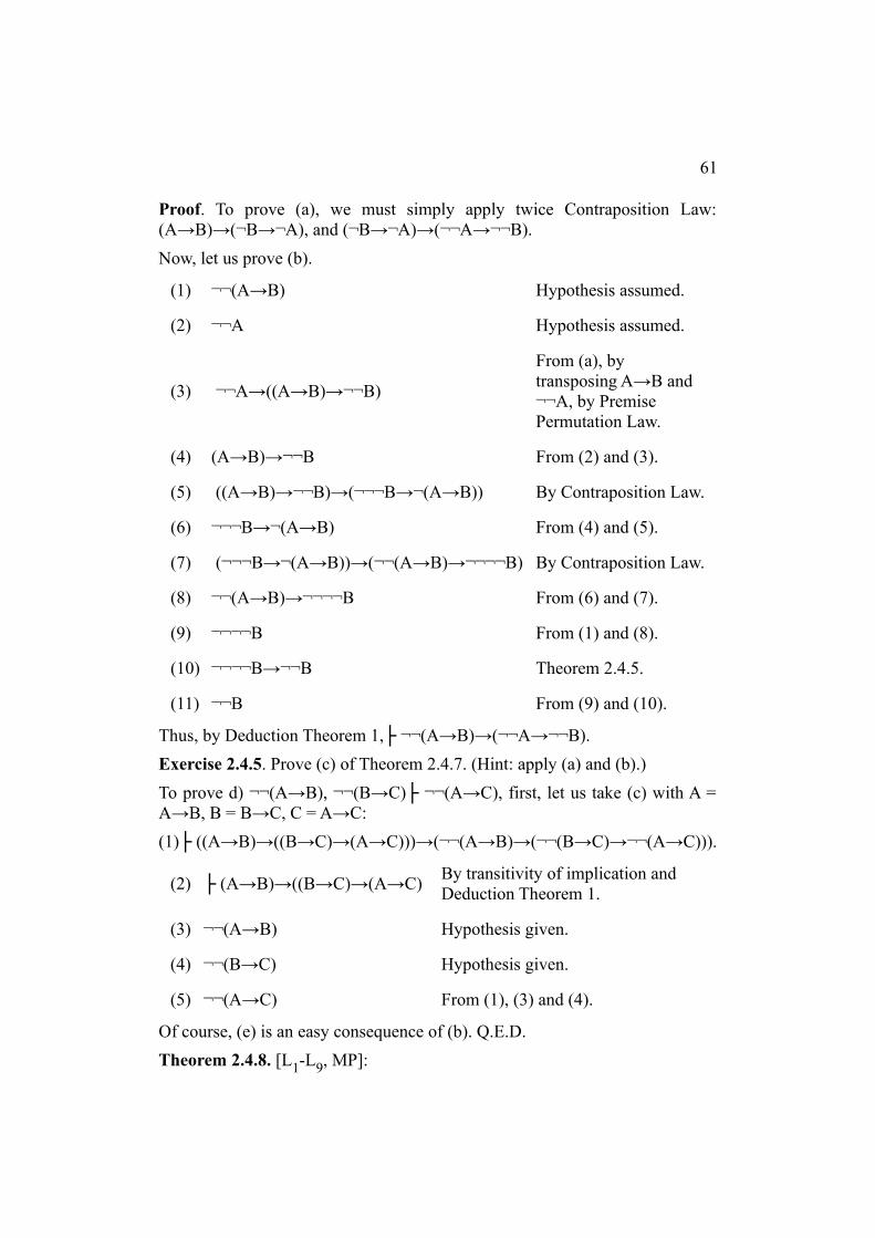
61

Proof. To prove (a), we must simply apply twice Contraposition Law:(A→B)→(¬B→¬A), and (¬B→¬A)→(¬¬A→¬¬B).

Now, let us prove (b).

(1) ¬¬(A→B) Hypothesis assumed.

(2) ¬¬A Hypothesis assumed.

(3) ¬¬A→((A→B)→¬¬B)

From (a), by transposing A→B and ¬¬A, by Premise Permutation Law.

(4) (A→B)→¬¬B From (2) and (3).

(5) ((A→B)→¬¬B)→(¬¬¬B→¬(A→B)) By Contraposition Law.

(6) ¬¬¬B→¬(A→B) From (4) and (5).

(7) (¬¬¬B→¬(A→B))→(¬¬(A→B)→¬¬¬¬B) By Contraposition Law.

(8) ¬¬(A→B)→¬¬¬¬B From (6) and (7).

(9) ¬¬¬¬B From (1) and (8).

(10) ¬¬¬¬B→¬¬B Theorem 2.4.5.

(11) ¬¬B From (9) and (10).

Thus, by Deduction Theorem 1,├ ¬¬(A→B)→(¬¬A→¬¬B).

Exercise 2.4.5. Prove (c) of Theorem 2.4.7. (Hint: apply (a) and (b).)

To prove d) ¬¬(A→B), ¬¬(B→C)├ ¬¬(A→C), first, let us take (c) with A =A→B, B = B→C, C = A→C:

(1)├ ((A→B)→((B→C)→(A→C)))→(¬¬(A→B)→(¬¬(B→C)→¬¬(A→C))).

(2) ├ (A→B)→((B→C)→(A→C)By transitivity of implication and Deduction Theorem 1.

(3) ¬¬(A→B) Hypothesis given.

(4) ¬¬(B→C) Hypothesis given.

(5) ¬¬(A→C) From (1), (3) and (4).

Of course, (e) is an easy consequence of (b). Q.E.D.

Theorem 2.4.8. [L1-L9, MP]:

62

a) ¬¬( A∧B)↔(¬¬A∧¬¬B) . What does it mean?

b) ¬¬ A∨¬¬ B →¬¬( A∨B) . What does it mean?

Exercise 2.4.6. a) Prove Theorem 2.4.8(a). (Hint: apply Contraposition Law –several times, and Theorem 2.4.7(b).)

b) Prove Theorem 2.4.8(b). (Hint: apply D-elimination, D-introduction andContraposition Law.)

Attention: non-constructive reasoning! The converse of (b):¬¬( A∨B)→¬¬ A∨¬ ¬ B cannot be proved in the constructive logic (see

Section 2.8). If we simply succeed in deriving a contradiction from¬(A∨B) , then, perhaps, we do not have a method allowing to decide,

which part of ¬¬ A∨¬¬ B is true – ¬¬A, or ¬¬B?

Augustus de Morgan (1806-1871): "He recognised the purely symbolic nature of algebra andhe was aware of the existence of algebras other than ordinary algebra. He introduced deMorgan's laws and his greatest contribution is as a reformer of mathematical logic."(according to MacTutor History of Mathematics archive).

Theorem 2.4.9.

a) [L1, L2, L8, L9, MP]: ¬A∨¬B →¬( A∧B) . It's the constructive half of

the so-called First de Morgan Law. What does it mean?

b) [L1-L9, MP]: ¬(A∨B)↔¬A∧¬B . It's the so-called Second de Morgan

Law. What does it mean?

Attention: non-constructive reasoning! The second half of (a) – the converseimplication ¬(A∧B)→¬A∨¬B can be proved in the classical logic, butnot in the constructive logic (see Section 2.8). Explain, why.

Proof. Let us prove (a).

(1) ¬ A∨¬ B Hypothesis assumed.

(2) A∧B Hypothesis (N-elimination).

(3) A C-elimination from (2).

(4) B C-elimination from (2).

(5) ¬A D-elimination from (1) ¬B D-elimination from (1)

(6) A ;¬A Contradiction. B ;¬B Contradiction.

(7)¬A ;¬¬A Unified

contradiction.¬A ;¬¬A Unified contradiction.

The last step is necessary, if we wish to apply D-elimination theorem. In this

63

theorem, it is supposed that in both branches a common formula is derived,and not two different ones. To unify both contradictions, we applied here the“50% L10 theorem” (“contradiction implies that all is wrong”) proved in

Exercise 1.4.2: [L1, L9, MP]: B ;¬B ├ ¬A ;¬¬A . Since we are operating

in the minimal logic, we could not apply L10 itself.

Exercise 2.4.7. Prove Theorem 2.4.9(b). (Hint: apply N- and D-elimination,the above-mentioned contradiction-unification included.)

Q.E.D.

Exercise 2.4.8. Prove:

a) [L1-L9, MP]: (A→ B)→ ¬( A∧¬ B) . What does it mean? Compare with

Theorem 2.4.2(b): A∧¬B →¬( A → B) .

b) [L1-L8, MP]: A∨B →(( A →B)→ B) . What does it mean?

Attention: non-constructive reasoning! The converse implications of (a, b),¬(A∧¬ B)→( A → B) and (( A→ B)→ B)→ A∨B cannot be proved in

the constructive logic (see Section 2.8). Explain, why. Still, we will provethese formulas in the classical logic.

2.5. Formulas Containing Negation – Constructive Logic

In this book, constructive logic is used as a synonym of intuitionistic logic!

Constructive logic includes the axiom L10: ¬B→(B→C), but rejects the Law

of Excluded Middle L11: B∨¬B as a general logical principle.

Exercise 2.5.1. a) [L10, MP]: A, ¬A├ B. What does it mean?

b) [L1, L2, L8, L10, MP]: A∨B →(¬ A→ B) . What does it mean?

We will verify in Section 2.8 that the formula (b) cannot be proved in theminimal logic [L1-L9, MP] (and even not in [L1-L9, L11, MP]), i.e., it cannot

be proved without L10.

Attention: non-constructive reasoning! The converse of (b), i.e.,(¬ A→ B)→ A∨B cannot be proved in the constructive logic (see Section

2.8). Explain, why.

Theorem 2.5.1. a) [L1, L8, L10, MP]: ¬A∨B →( A→ B) . What does it

mean?

64

b) [L1, L2, L6, MP]: A∨B →(¬A → B) ├ ¬A→(A → B) . What does it

mean? It means that the “natural” rule A∨B ;¬ A ├ B implies L10!

We will verify in Section 2.8 that the formula Theorem 2.5.1(a) cannot beproved in the minimal logic [L1-L9, MP] (and even not in [L1-L9, L11, MP]),

i.e., it cannot be proved without L10.

Attention: non-constructive reasoning! The converse of (a), i.e.,(A → B)→¬ A∨B cannot be proved in constructive logic (see Section 2.8).

Explain, why.

Proof. a) When proving (a), we cannot use Deduction Theorem 1 (because ofthe missing axiom L2). So, let us simply build a sequence of 5 formulas

representing the proof of (a):

(1)(¬A→(A → B))→((B →( A→ B))→(¬A∨B →( A→ B)))

(Axiom L8)

(2) ¬A→(A → B) Axiom L10.

(3) B →( A→ B) Axiom L1.

(4)(B →( A→ B))→

(¬A∨B →(A → B)) By MP, from (1), (2).

(5) ¬A∨B →( A→ B) By MP, from (4), (3).

b) Surprisingly, the rule A∨B ,¬ A ├ B seems to be a quite a "natural"logical principle, yet it cannot be proved without the axiom L10! Why not?

Because it implies L10! Indeed,

(1) A∨B →(¬ A→ B) Hypothesis given.

(2) ¬AHypothesis assumed (¬A→(A→B) to prove!)

(3) A Hypothesis assumed.

(4) A∨B By D-introduction, from (3).

(5) B By MP, from (1), (4) and (2).

Hence, by Deduction Theorem 1,

65

[L1, L2, L6, MP]: A∨B →(¬ A → B) ├ ¬A→(A→B). Q.E.D.

Theorem 2.5.2. [L1-L10, MP]:

a) (¬¬A→¬¬B)→¬¬(A→B). It's the converse of Theorem 2.4.7(b). Hence,[L1-L10, MP]:├ ¬¬(A→B)↔(¬¬A→¬¬B).

b) ¬¬A→(¬A→A). It's the converse of Theorem 2.4.6(a). Hence, [L1-L10, MP]: ¬¬A↔(¬A→A).

c) A∨¬ A →(¬ ¬ A → A) . What does it mean?

d) ¬¬(¬¬A→A). What does it mean? It’s a “weak” form of the DoubleNegations Law – provable in constructive logic.

We will verify in Section 2.8 that formulas (a, b, c, d) cannot be proved in theminimal logic [L1-L9, MP] (and even not in [L1-L9, L11, MP]), i.e., they

cannot be proved without L10.

Proof. Of course, (b) is an instance of the axiom L10.

To prove (a), prove in Exercise 2.5.2 that ¬¬A→¬¬B, ¬(A→B)├ ¬B, ¬¬B.Then, by N-elimination theorem,├ (¬¬A→¬¬B)→¬¬(A→B).

To prove (c) and (d) do Exercise 2.5.2(b). Q.E.D.

Exercise 2.5.2. a) Prove that [L1-L10, MP]: ¬¬A→¬¬B, ¬(A→B)├ ¬B, ¬¬B.

b) Prove (c) and (d) of Theorem 2.5.2.

Exercise 2.5.3. Prove that in [L1-L10, MP]:

a) A├ B ↔ B∨¬ A . What does it mean?

b) B∨( A∧¬ A)↔B . What does it mean?

c) (( A∧¬ A)∧B)∨C ↔C . What does it mean?

2.6. Formulas Containing Negation – Classical Logic

If you agree to adopt the axiom L11: B∨¬ B , i.e., the Law of Excluded

Middle, you can prove, first of all:

Theorem 2.6.1. (Double Negation Law)

[L1, L2, L8, L10, L11, MP]: ¬¬A → A.

Hence, [L1-L11, MP]: ¬¬A ↔ A.

66

Exercise 2.6.1. Prove Theorem 2.6.1.

We will verify in Section 2.8 that the formula ¬¬A → A cannot be proved inthe minimal logic [L1-L9, MP] (and even not in [L1-L9, L11, MP]), i.e., it

cannot be proved without L10.

In the minimal logic we proved Theorem 2.4.4: [L1, L2, L9, MP]: A→¬¬A.

Hence, [L1-L11, MP]: ¬¬A ↔ A.

Attention: non-constructive reasoning! The formula ¬¬A→A cannot beproved in the constructive logic, see Section 2.8. Why? Because it represents akind of non-constructive reasoning. Indeed, imagine, you wish to prove that

xB(x). Assume the contrary, ¬ xB(x), and derive a contradiction. Thus you∃z(x+z+1=y). ∃z(x+z+1=y).have proved the negation of ¬ xB(x), i.e., ¬ ¬ xB(x). To conclude xB(x)∃z(x+z+1=y). ∃z(x+z+1=y). ∃z(x+z+1=y).from ¬ ¬ xB(x), you need the Double Negation Law. Hence, by adopting this∃z(x+z+1=y).law as a logical principle, you would allow non-constructive existence proofs– if you prove xB(x) by assuming ¬ xB(x), and deriving a contradiction,∃z(x+z+1=y). ∃z(x+z+1=y).then you may not obtain a method allowing to find a particular x satisfyingB(x).

Theorem 2.6.2. [L8, L11, MP]: A→B, ¬A→B├ B. Or, by Deduction Theorem

1, [L1, L2, L8, L11, MP]: (A→B)→((¬A→B)→B). What does it mean?

This formula cannot be proved in the constructive logic (see Section 2.8).Explain, why.

Exercise 2.6.2. Prove Theorem 2.6.2.

In the classical logic, you can prove also the converse of ContrapositionLaw:

Theorem 2.6.3. [L1-L11, MP]: (¬B→¬A)→(A→B). Hence, [L1-L11, MP]:

(A→B) ↔ (¬B→¬A).

Attention: non-constructive reasoning! The formula (¬B→¬A)→(A→B)cannot be proved in the constructive logic, see Section 2.8. Explain, why.

Exercise 2.6.2. Prove that in [L1-L11, MP]:

a) Theorem 2.6.3. (Hint: apply Double Negation Law.)

b) (¬A→B)↔(¬B→A). Compare with Exercise 2.4.3(b): [L1-L9, MP]:

(A→¬B)↔(B→¬A).

Attention: non-constructive reasoning! The formula (b) cannot be proved inthe constructive logic, see Section 2.8.

Theorem 2.6.3. [L1-L9, L11, MP]: ˫ ¬(A∧B)→¬A∨¬B . Hence, [L1-L9,

67

L11, MP]: ˫ ¬(A∧B)↔¬A∨¬B .

The equivalence represents the First de Morgan Law.

Let us remind also the Second de Morgan Law:

[L1-L9, MP]: ¬(A∨B)↔¬ A∧¬ B .

Thus, both of de Morgan laws can be proved in [L1-L9, L11, MP], i.e., they do

not depend on the axiom L10.

Proof. The constructive half of the First Law we proved in the minimal logicas Theorem 2.4.9(a): [L1-L9, MP]: ¬ A∨¬ B → ¬(A∧B) . Let us prove the

remaining half: [L1-L9, L11, MP]: ¬( A∧B)→¬ A∨¬ B . The axiom L10

will not be used in this proof.

Let us apply a pretty general method of proving formulas in the classicallogic: start the proof by introducing instances of L11 as hypotheses and

applying D-elimination.

Our particular proof starts by assuming (0) ¬( A∧B) as the hypothesis, afterthis we introduce A∨¬A ; B∨¬B as additional hypotheses. Then, by D-elimination, we obtain 4 branches starting with the following hypotheses:

1) A ;B , 2) A ;¬B , 3) ¬A ; B , 4) ¬A;¬B .

In branches (2, 3, 4) we obtain the required formula ¬ A∨¬ B simply by D-introduction.

In the branch (1):

(1) A Hypothesis assumed.

(2) B Hypothesis assumed.

(3) A∧BBy C-introduction, from (1), (2). Contradiction with our initial hypothesis: (0) ¬( A∧B) .

(4) ¬ A

From (0) and (3), but not by L10!

By[L1, L9, MP]: B, ¬B├ ¬C, proved

in Exercise 1.4.2.

(5) ¬ A∨¬B By D-introduction, from (4).

Thus, we have proved 4 cases:

[L1-L9, MP]: ¬(A∧B); xA; yB ├ ¬A∨¬B ,

68

where each of x, y is either an empty symbol, or a negation symbol. By D-elimination theorem, we obtain 2 cases:

[L1-L9, MP]: ¬(A∧B); xA; B∨¬B ├ ¬A∨¬B ,

and, finally: [L1-L9, MP]: ¬(A∧B); A∨¬B ; B∨¬B ├ ¬A∨¬B and

[L1-L9, L11, MP]: ¬(A∧B) ├ ¬A∨¬B . Q.E.D.

It appears that, in the classical logic, we can express implication by usingnegation and disjunction (let us call it I-elimination). Indeed, we alreadyknow that [L1, L8, L10, MP]: ¬ A∨B →( A→ B) (Theorem 2.5.1).

Exercise 2.6.3. Prove that [L1-L8, MP]: A∨C ├ (A→ B)→ B∨C .

Hence, [L1-L8, MP]: A∨¬ A ├ (A→ B)→¬ A∨B , i.e.,

Theorem 2.6.4. [L1-L8, L11, MP]: (A→ B)→ ¬ A∨B . Hence,

(I-elimination) [L1-L11, MP]: (A→ B)↔ ¬ A∨B .

Exercise 2.6.4. Prove that in [L1-L11, MP]:

a) B∧( A∨¬ A)↔ B . What does it mean?

b) (( A∨¬ A)∨B)∧C ↔C . What does it mean?

c) (( A→ B)→ B)→ A∨B . What does it mean? By adding the result ofExercise 2.4.7, [L1-L11, MP]: A∨B ↔((A → B)→ B) .Thus, in the classical

logic, disjunctions can be replaced by implications.

Theorem 2.6.5. [L1-L11, MP]: ¬(A→ B)→ A∧¬B .

Hence, together with Theorem 2.4.2(b): [L1-L11, MP]: ¬(A→ B)↔ A∧¬B .

Proof. Do Exercise 2.6.5(b).

Thus, in the classical logic, an implication is false if and only if the premise istrue, and the conclusion is false.

In the constructive logic, if an implication is false, it follows only that theconclusion is false. Indeed, from L1: B →( A→ B) , by Contraposition Law:

[L1, L2, L9, MP]: ¬(A→ B)→¬B . But the formula ¬(A→ B)→ A can

be proved in the classical logic only (see Theorem 2.8.5 in Section 2.8).

Exercise 2.6.5. Prove that in [L1-L11, MP]:

a) (A → B)↔¬( A∧¬ B) . What does it mean?

b) ¬(A → B)↔ A∧¬ B .

69

c) A∨B ↔(¬ A→ B) . What does it mean?

d) A∧B ↔¬( A→ ¬ B) . What does it mean?

e) (optional, for smart students) Try detecting, which parts of theseequivalences are provable in the constructive logic. (Hint: take a look atTheorem 2.8.5.)

Strange formulas

Exercise 2.6.6. Prove in the classical logic the following strange formulas.(Hint: the easy way – apply the method used above to prove Theorem 2.6.3.)

a) [L1, L2, L6–L 8, L10, L11, MP]: A∨( A→ B) . What does it mean? Does it

mean anything at all? Compare with Exercise 1.4.2.

b) [L1, L2, L6–L8, L10, L11, MP]: (A → B)∨( B → A) . What does it mean?

Does it mean anything at all?

c) [L1–L11, MP]: (( A→ B)→ A)→ A . What does it mean? Does it mean

anything at all? It is the so-called Peirce's Law from:

C. S. Peirce. On the algebra of logic: A contribution to the philosophy of notation. AmericanJournal of Mathematics, 1885, vol.7, pp.180-202.

2.7. Constructive Embedding: Glivenko's Theorem

Let us remind some of the results of previous sections concerning doublenegations:

Theorem 2.4.4. [L1, L2, L9, MP]: A→¬¬A.

Theorem 2.4.5. [L1–L9, MP]: ¬¬¬A↔¬A.

Theorem 2.4.6(b). [L1–L9, MP]: ¬¬( A∨¬ A) . In this weak form, the Law

of Excluded Middle can be proved constructively.

Theorem 2.4.7. [L1–L9, MP]: a) (A→B)→(¬¬A→¬¬B).

b) ¬¬(A→B)→(¬¬A→¬¬B).

c) (A→(B→C))→(¬¬A→(¬¬B→¬¬C)).

d) ¬¬(A→B), ¬¬(B→C)├ ¬¬(A→C).

e) ¬¬A, ¬¬(A→B)├ ¬¬B.

Theorem 2.4.8. [L1-L9, MP]:

a) ¬¬( A∧B)↔ (¬¬ A∧¬¬ B) .

70

b) ¬¬ A∨¬¬ B →¬¬( A∨B) .

Theorem 2.5.2. [L1-L10, MP]:

a) (¬¬A→¬¬B)→¬¬(A→B). It's the converse of Theorem 2.4.7(b).

d) ¬¬(¬¬A→A).

Theorem 2.6.1. [L1-L11, MP]: ¬¬A ↔ A.

Does it mean that for any formula A:

If [L1-L11, MP]:├ A, then [L1-L10, MP]:├ ¬¬A?

(The converse is obvious: if [L1-L10, MP]:├ ¬¬A, then [L1-L11, MP]:├ A by

Theorem 2.6.1.)

Imagine, we have a proof of [L1-L11, MP]:├ A. It is a sequence of formulas

R1, R2, ..., Rn, where Rn = A. If this sequence does not contain instances of the

axiom L11, then it is a proof of [L1-L10, MP]:├ A as well. Hence, according to

Theorem 2.4.4, [L1-L10, MP]:├ ¬¬A

If the sequence R1, R2, ..., Rn contains some instances of L11, i.e., formulas

having the form B∨¬ B , then, according to Theorem 2.4.6(b), we could tryreplacing each such formula by a sequence proving that [L1-L9, MP]:

¬¬(B∨¬ B) . It appears that each of the formulas ¬¬R1, ¬¬R2, ..., ¬¬Rn is

provable in [L1-L10, MP].

a) If Rk is an instance of the axioms L1-L10, then [L1-L10, MP]:├ ¬¬Rk

(Theorem 2.4.4).

b) If Rk is an instance of the axiom L11, then [L1-L10, MP]:├ ¬¬Rk (Theorem

2.4.6(b)).

c) Now, let us assume that i, j < k, and Ri, Rj├ Rk directly by MP, i.e., Rj is

Ri→Rk. We know already that [L1-L10, MP]:├ ¬¬Ri and [L1-L10, MP]:├

¬¬(Ri→Rk). By Theorem 2.4.7(b),

[L1-L9, MP]:├ ¬¬(Ri→Rk)→ (¬¬Ri→¬¬Rk).

Hence, [L1-L10, MP]:├ ¬¬Rk.

Because A = Rn, we have proved the remarkable Glivenko's theorem from

1929:

V. Glivenko. Sur quelques points de la logique de M. Brouwer. Academie Royale de Belgique,Bulletins de la classe des sciences, 1929, ser.5, vol.15, pp.183-188.

71

Valery Ivanovich Glivenko (1897-1940) is best known by the so-called Glivenko-Cantellitheorem in probability theory.

Theorem 2.7.1 (Glivenko's Theorem).

[L1-L11, MP]:├ A if and only if [L1-L10, MP]:├ ¬¬A.

Or: a formula A is provable in the classical propositional logic if and only if itsdouble negation ¬¬A is provable in the constructive propositional logic.

This theorem provides a kind of a "constructive embedding" for the classicalpropositional logic: any classically provable formula can be "proved" in theconstructive logic, if you put two negations before it.

Corollary 2.7.1. [L1-L11, MP]:├ ¬A if and only if [L1-L10, MP]:├ ¬A.

Or: a "negative" formula ¬A is provable in the classical propositional logic ifand only if it is provable in the constructive propositional logic.

Indeed, if [L1-L11, MP]:├ ¬A, then by Glivenko's theorem, [L1-L10, MP]:├

¬¬¬A, and by Theorem 2.4.5, [L1-L10, MP]:├ ¬A. Q.E.D.

Exercise 2.7.1. Prove the following version of Glivenko's theorem (see Kleene[1952]):

a) If [L1-L11, MP]: A1, A2, ..., An├ C, then

[L1-L10, MP]: ¬¬A1, ¬¬A2, ..., ¬¬An├ ¬¬C.

b) If [L1-L11, MP]: ¬A1, ¬A2, ..., ¬An, B1, B2, ..., Bp├ ¬C, then

[L1-L10, MP]: ¬A1, ¬A2, ..., ¬An , ¬¬B1, ¬¬B2, ..., ¬¬Bp├ ¬C.

2.8. Axiom Independence. Using Computers in Mathematical Proofs

If one of our axioms Li could be proved by using the other axioms only, then

we could simplify our logical system by dropping Li as an axiom. A striking

example:

Theorem 2.8.1. The axiom L9: (A→B)→((A→¬B)→¬A) can be proved in

[L1, L2, L8, L10, L11, MP].

This fact was established by Augusts Kurmītis (on the web, also: A. A. Kurmit):

A. A. Kurmitis. On independence of a certain axiom system of the propositional calculus.Proc. Latvian State University, 1958, Vol. 20, N3, pp. 21-25 (in Russian).

72

The following proof of L9 in [L1, L2, L8, L10, L11, MP] is due to Jānis Sedols.

First, let us establish that the formula (A→¬A)→¬A can be proved in [L1, L2,

L8, L10, L11, MP] (in Exercise 2.4.1 we established that [L1, L2, L9, MP]:

(A→¬A)→¬A):

(1) (A →¬ A)→((¬ A →¬ A)→( A∨¬ A)→¬ A) Axiom L8.

(2) A→¬A Hypothesis.

(3) ¬A→¬AThis is provable in [L1, L2,

MP] (Theorem 1.4.1).

(4) A∨¬ A Axiom L11.

(4) ¬AFrom (1), (2), (3) and (4), by MP.

(6) (A→¬A)→¬A

By Deduction Theorem 1 (which is valid for any propositional system containing [L1, L2, MP]).

Now let us establish that in [L1, L2, L10, MP]: A→B, A→¬B├ A→¬A.

(7) A→B Hypothesis.

(8) A→¬B Hypothesis.

(9) A Hypothesis.

(9) B From (7), (9), by MP.

(10) ¬B From (8), (9), by MP.

(11) ¬B→(B→¬A) Axiom L10.

(12) ¬A From (9), (10) and (11) by MP.

(13) A→B, A→¬B├ A→¬ABy Deduction Theorem 1 (which is valid for any propositional system containing [L1, L2, MP]).

Finally, let us merge the proofs of (6) and (13), then by MP we obtain ¬A, i.e.,

[L1, L2, L8, L10, L11, MP]: A→B, A→¬B├ ¬A.

73

Now, by Deduction Theorem 1 (which is valid for any propositional systemcontaining [L1, L2, MP]) we obtain the axiom L9:

[L1, L2, L8, L10, L11, MP]: (A→B)→((A→¬B)→¬A).

Q.E.D.

What should we do after establishing that one of our axioms is "dependent"?Do you think, we should drop L9 as an axiom of our logical system?

First, let's note that we have proved L9 by using three problematic axioms:

L1, L10, L11. But L9 itself is not problematic!

Secondly, L9 cannot be proved in [L1-L8, L10, MP] (see Theorem 2.8.2

below). Hence, if we would drop L9, then, instead of a simple definition

classical logic = constructive logic + L11,

we would need a more complicated one:

constructive logic = classical logic – L11 + L9.

So, let us retain L9 in our list of logical axioms.

But now, the question of questions:

Is the Law of Excluded Middle an independent logical principle?

Are constructive logic and classical logic really different? Of course, they are,but how could one prove that?

Could we prove the Law of Excluded Middle (the axiom L11: B∨¬ B ) by

using the other axioms [L1-L10, MP] – as we proved L9 in [L1, L2, L8, L10,

L11, MP]? If not, how could we demonstrate that this is impossible? How

could we demonstrate that some logical principle is independent, i.e., that itcannot be derived from other principles?

Let us assume, we have designed an algorithm q that calculates for eachformula A some its "property" q(A) in such a way that:

a) q(L1) is true, q(L2) is true, ..., q(L10) is true (i.e., the axioms L1-L10 possess

the property q).

b) If q(A) is true and q(A→B) is true, then q(B) is true (i.e., Modus Ponens"preserves" the property q).

If so, then q(F) is true for all the formulas F that can be proved in [L1-L10,

MP].

74

c) q(L11) is false (i.e., L11 does not possess the property q).

If we could develop such an algorithm q, then this would demonstrate that L11

cannot be proved in [L1-L10, MP], i.e., that the Law of Excluded Middle is an

independent logical principle.

Multi-valued logics

One of the ways way how to introduce remarkable properties of formulas arethe so-called "multi-valued logics" or "many-valued logics", introduced by JanLukasiewicz and Emil Post:

J. Lukasiewicz. O logice trojwartosciowej. Ruch Filozoficzny (Lwow), 1920, vol. 5, pp. 169-171

E. Post. Introduction to a general theory of elementary propositions. Amer. journ. math., 1921,vol. 21, pp.163-195

Read more: Many-Valued Logic by Siegfried Gottwald in Stanford Encyclopedia ofPhilosophy.

For example, let us consider a kind of "three-valued logic", where 0 means"false", 1 – "unknown" (or NULL – in terms of SQL), and 2 means "true".Then it would be natural to define “truth values” of conjunction anddisjunction as

A∧B=min( A , B) ;A∨B=max(A , B) .

But how should we define “truth values” of implication and negation?

A B A∧B A∨B A→B

0 0 0 0 i1

0 1 0 1 i2

0 2 0 2 i3

1 0 0 1 i4

1 1 1 1 i5

1 2 1 2 i6

2 0 0 2 i7

2 1 1 2 i8

75

2 2 2 2 i9

A ¬A

0 i10

1 i11

2 i12

Thus, theoretically, we have here 39 = 19683 variants of implicationdefinitions and 33 = 27 negation definitions.

Do you think, it would be natural to set the values of ¬A and A→B as follows?

A ¬A

0 2

1 1

2 0

A B A→B

0 0 2

0 1 2

0 2 2

1 0 1

1 1 1

1 2 2

2 0 0

2 1 1

2 2 2

Yes, it would be natural, if we would try building a natural three-valued logic,in which "1" would mean, indeed, "unknown". In this way we would obtain

76

the “natural” three-valued logic used, for example, for handling of NULL-values in SQL.

However, for our purpose, we must separate two different classes of formulasprovable in the classical logic. For this task, the above “natural” logic isuseless: under it, the axioms L1- L11 “behave” irregularly (verify).

Thus, here, our aim must be just the opposite to inventing of a “natural” logic– creating of a “bad” logic.

Let us consider

"under our truth tables, formula A always takes "true" values (the value 2)"

as a kind of the above-mentioned "property" q(A). We are trying to prove thatthe axiom L11 cannot be derived from the axioms L1- L10. Hence, we must try

to define our truth tables in such a way that:

a) the axioms L1, L2, ..., L10 always take the value 2,

b) Modus Ponens preserves taking always the valuec2 (i.e., if the formulas Aand A→B are always 2, then B also is always 2),

c) the axiom L11 sometimes takes the value 0 or 1.

As we saw above, the truth tables, having these properties, cannot be 100%natural. So, we must explore the "unnatural" versions as well.

However, let us retain the “natural” definitions of conjunction and disjunction:

A∧B=min( A , B) ;A∨B=max(A , B) .

Exercise 2.8.1 (optional). Develop a simple (recursive) computer program receiving as input:

a) any truth tables of implication and negation,

b) Any formula F consisting of letters A, B, C, propositional connectives and parentheses,

and printing out "truth values" of the formula F, for example, if F = B→(A→B):

A B B→(A→B)

0 0 2

0 1 2

0 2 2

1 0 2

1 1 2

77

1 2 2

2 0 2

2 1 2

2 2 2

In this example the axiom L1 always takes "true" values. Perhaps, we should be interested

only in those variants of our truth tables that "satisfy" at least the axioms L1, L2, ..., L8 forcing

them always to take "true" values.

Thus, we consider

"under the selected truth tables, formula A always takes "true" values"

as a kind of the "property" q(A).

Will MP preserve this property? If A is "true", and A→B is "true", how couldB be not? Let us consider the relevant part of the truth table for implication(the part where A is "true"):

A B A→B

2 0 i7 i7=0,1

2 1 i8 i8=0,1

2 2 i9 2

If we would consider only those variants of our truth tables where i7 = 0 or 1,

i8 = 0 or 1, and i9 = 2, then, if B would not be 2 for some values of its

arguments, then A→B also would not be 2 for the same values of arguments.

Hence, if we restrict ourselves to truth tables with i7 = 0 or 1, i8 = 0 or 1, and

i9 = 2, then MP preserves the property of "being true". i.e., from "true"

formulas MP will derive only "true" formulas.

The next idea: if we wish the axiom L6: A→ A∨B always taking the value

2, then, if A≤B, then A→B must be 2.

Thus, of all the 39 = 19683 possible implication definition variants only thefollowing 3*2*2 = 12 variants are worth of exploring:

A B A→B

0 0 2

78

0 1 2

0 2 2

1 0 i4=0,1,2

1 1 2

1 2 2

2 0 i7=0,1

2 1 i8=0,1

2 2 2

Exercise 2.8.2. a) Verify that under any of these 12 implication definitions theaxioms L3, L4, L6, L7 always take the value 2, i.e., you do not need testing

these axioms any more.

b) For each of the axioms, L1, L2, L5 and L8, determine all the possible

combinations of the values of i4, i7, i8 forcing it to take always the value 2.

Note. The "intersection" of b) consists of 5 variants only.

Exercise 2.8.3 (optional) Extend your previous computer program by adding 6nested loops: for i4=0 to 2, for i7=0 to 1, for i8=0 to1, for iaa=0 to 2, for ib=0 to

2, for ic=0 to 2. Let the program print out only those variants of truth tables

that make "true" all the axioms L1-L8. (My own program produced 135 such

variants, see the results file #00).

Thus, now we have 135 variants of truth tables which make "true" all theaxioms L1-L8 and for which “truth” is retained when MP is applied. So, let us

search among them for the variants that allow proving of axiom independenceresults we are interested in.

Axiom L9

In Theorem 2.8.1 we established that the axiom L9: (A→B)→((A→¬B)→¬A)

can be proved in [L1-L8, L10, L11, MP]. Still,

Theorem 2.8.2. The axiom L9 cannot be proved in [L1-L8, L10, MP].

Proof. Let your program print out only those variants of truth tables that make"true" all the axioms L1-L8, and make: L9 – not "true", and L10 – "true". My

program yields 66 such variants, see the results file #01. Let us consider, for

79

example, the variant #33 (the unnatural clauses are marked bold):

Implication variant #3:2 2 2 2 2 2 0 1 2 L1-L8 true. Variant #33. Negation: 2 1 0 L9 not true. L10 true. L11 not true.

A B A→B

0 0 2

0 1 2

0 2 2

1 0 2

1 1 2

1 2 2

2 0 0

2 1 1

2 2 2

A ¬A

0 2

1 1

2 0

See the extended results file #1 for this variant.

Under this variant the axioms L1-L8 and L10 are "true". As we know, under

this variant, by MP, from "true" formulas only "true" formulas can be derived.The axiom L9 is not "true" under this variant:

A B (A→B)→((A→¬B)→¬A)

0 0 2

0 1 2

0 2 2

80

1 0 1

1 1 1

1 2 1

2 0 2

2 1 2

2 2 2

Hence, L9 cannot be proved in [L1-L8, L10, MP]. Q.E.D.

In a similar way, we can obtain some other independence results as well.

Axiom L10

Theorem 2.8.3. The axiom L10: ¬B→(B→C) cannot be proved in the minimal

logic [L1-L9, MP], and even not in [L1-L9, L11, MP].

Proof. Let your program print out only those variants of truth tables that make"true" all the axioms L1-L8, and make: L9 – "true", L10 – not "true", and L11 –

"true". My program yields 6 such variants, see the results file #02. Let usconsider, for example, the variant #1 (the unnatural clauses are marked bold):

Implication variant #1:2 2 2 0 2 2 0 1 2 L1-L8 true. Variant #1. Negation: 2 2 1 L9 true. L10 not true. L11 true.

See the extended results file #2 for this variant.

Under this variant the axioms L1-L9 and L11 are "true". As we know, under

this variant, by MP, from "true" formulas only "true" formulas can be derived.The axiom L10 is not "true" under this variant:

A B ¬A→(A→B)

0 0 2

0 1 2

0 2 2

1 0 2

1 1 2

81

1 2 2

2 0 0

2 1 1

2 2 2

Hence, L10 cannot be proved in [L1-L9, L11, MP]. Q.E.D.

Axiom L11

Now, let us prove the main result of this section:

Theorem 2.8.4. The Law of Excluded Middle L11: B∨¬ B cannot be

proved in the constructive propositional logic [L1-L10, MP]. The Law of

Excluded Middle is an independent logical principle.

Proof. Let your program print out only those variants of truth tables that make"true" all the axioms L1-L8, and make: L9 – "true", L10 – "true", L11 – not

"true". My program yields only one such variant, see the results file #03:

Implication variant #1 (the unnatural clauses are marked bold):2 2 2 0 2 2 0 1 2 L1-L8 true. Variant #1. Negation: 2 0 0 L9 true. L10 true. L11 not true.

See the extended results file #3 for this variant. (As we see, the implicationdefinition coincides here with the one used above to “discredit” L10, but the

negation definition is different.)

Under this variant the axioms L1-L10 are "true". As we know, under this

variant, by MP, from "true" formulas only "true" formulas can be derived. Theaxiom L11 is not "true" under this variant:

B ¬B B∨¬ B

0 2 2

1 0 1

2 0 2

Hence, L11 cannot be proved in [L1-L10, MP]. Q.E.D.

The results file #03 proves also the following

Theorem 2.8.5 (thanks to Pavels Mihailovs for a correction). The followingclassically provable formulas cannot be proved in the constructive

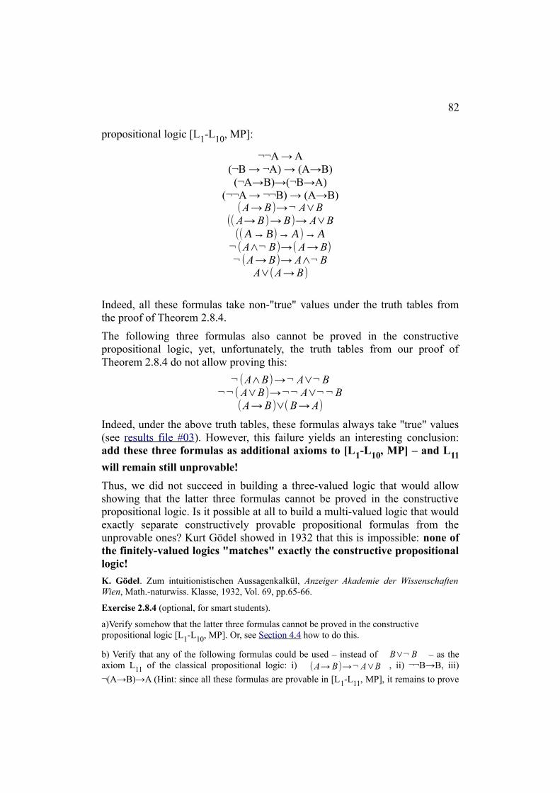
82

propositional logic [L1-L10, MP]:

¬¬A → A(¬B → ¬A) → (A→B)(¬A→B)→(¬B→A)

(¬¬A → ¬¬B) → (A→B)(A → B)→¬ A∨B

(( A→ B)→ B)→ A∨B((A→B)→A)→A

¬(A∧¬ B)→( A → B)¬(A → B)→ A∧¬ B

A∨(A → B)

Indeed, all these formulas take non-"true" values under the truth tables fromthe proof of Theorem 2.8.4.

The following three formulas also cannot be proved in the constructivepropositional logic, yet, unfortunately, the truth tables from our proof ofTheorem 2.8.4 do not allow proving this:

¬(A∧B)→¬ A∨¬ B¬¬( A∨B)→¬¬ A∨¬ ¬ B

(A → B)∨( B → A)

Indeed, under the above truth tables, these formulas always take "true" values(see results file #03). However, this failure yields an interesting conclusion:add these three formulas as additional axioms to [L1-L10, MP] – and L11

will remain still unprovable!

Thus, we did not succeed in building a three-valued logic that would allowshowing that the latter three formulas cannot be proved in the constructivepropositional logic. Is it possible at all to build a multi-valued logic that wouldexactly separate constructively provable propositional formulas from theunprovable ones? Kurt Gödel showed in 1932 that this is impossible: none ofthe finitely-valued logics "matches" exactly the constructive propositionallogic!

K. Gödel. Zum intuitionistischen Aussagenkalkül, Anzeiger Akademie der WissenschaftenWien, Math.-naturwiss. Klasse, 1932, Vol. 69, pp.65-66.

Exercise 2.8.4 (optional, for smart students).

a)Verify somehow that the latter three formulas cannot be proved in the constructive propositional logic [L1-L10, MP]. Or, see Section 4.4 how to do this.

b) Verify that any of the following formulas could be used – instead of B∨¬ B – as theaxiom L11 of the classical propositional logic: i) (A→ B)→ ¬ A∨B , ii) ¬¬B→B, iii)

¬(A→B)→A (Hint: since all these formulas are provable in [L1-L11, MP], it remains to prove

83

L11 in [L1-L10, MP] + (i), in [L1-L10, MP] + (ii), and in [L1-L10, MP] + (iii)).

c) Verify that with ¬¬B→B instead of L11 the axiom L10 becomes 100% derivable from the

other axioms. Perhaps, this is why many textbooks prefer the combination L1-L9 + ¬¬B→B as

the axiom list for the classical propositional logic. But, then, we are forced to define theconstructive propositional logic not as a subset of the classical one, but as the classical logicwith the axiom ¬¬B→B replaced by the axiom L10: ¬B→(B→C)!

Axiom L10 again...

Finally, let us check which of the main results of Section 2.5 (constructive logic) and Section 2 .6 (classical logic) depend on the axiom L10. Let your

program print out only those variants of truth tables that make "true" all the axioms L1-L8, and make: L9 – "true", L10 – not "true". My program yields 6

such variants, see the results file #04. Surprisingly, in all these variants L11 is

"true" (thus, the results file #04 equals the results file #02 ). As the most productive appears

Implication variant #1:2 2 2 0 2 2 0 1 2 L1-L8 true. Variant #1. Negation: 2 2 1 L9 true. L10 not true. L11 true.

Constructively provable formulas:Not true: (A∨B)→((¬ A)→ B)Not true: ((¬ A)∨B)→(A → B)Not true: ((¬¬A)→(¬¬B))→(¬¬(A→B))Not true: (¬¬A)→((¬A)→A)Not true: (A∨(¬ A))→ ((¬ ¬ A)→ A)Not true: ¬¬((¬¬A)→A)

Classically provable formulas:True: (¬¬( A∨B))→((¬¬ A)∨(¬ ¬ B))True: (¬(A∧B))→((¬ A)∨(¬ B))Not true: (¬¬A)→ANot true: ((¬B)→(¬A))→(A→B)Not true: ((¬A)→B)→((¬B)→A)Not true: ((¬¬A)→(¬¬B))→(A→B)True: (A → B)→ ((¬ A)∨B)Not true: (( A→ B)→ B)→ (A∨B)Not true: ((A→B)→A)→ANot true: (¬(A∧(¬ B)))→( A→ B)True: (A→B)→(((¬A)→B)→B)Not true: (¬(A → B))→( A∧(¬ B))Not true: A∨(A → B)

84

True: (A → B)∨( B → A)Not true: (A→B)→(((¬A)→(¬B))→(B→A))

Thus, the following constructively provable formulas cannot be proved in theminimal logic [L1-L9, MP] (and even not in [L1-L9, L11, MP]), i.e., they

cannot be proved without the axiom L10:

(A∨B)→(¬ A → B)¬ A∨B →( A→ B)

(¬¬A→¬¬B) → ¬¬(A→B)¬¬A → (¬A→A)

A∨¬ A →(¬¬ A → A)¬¬(¬¬A→A)

And the following classically provable formulas cannot be proved without theaxiom L10 (thanks to Pavels Mihailovs for a correction):

¬¬A→A(¬B→¬A)→(A→B)(¬A→B)→(¬B→A)

(¬¬A→¬¬B)→(A→B)(( A→ B)→ B)→ A∨B

((A→B)→A)→A¬(A∧¬ B)→( A → B)¬(A → B)→ A∧¬ B

A∨(A → B)(A→B)→((¬A→¬B)→(B→A))

But how about the remaining five (classically provable) formulas (thanks toStanislav Golubcov for the idea):

a) (A → B)→ ¬ A∨B ,b) ¬(A∧B)→¬ A∨¬ B ,c) ¬¬(A∨B)→¬¬ A∨¬¬ B ,d) (A→B)→((¬ A→B)→B) ,e) (A → B)∨( B → A) ?

Formulas (a, b, d) can be proved without without L10, see Section 2.6.

Exercise 2.8.5. Show that also the formula (c) can be proved without L10, i.e

prove it in [L1-L9, L11, MP]. Smart students: how about the remaining formula

(e)?

Using computers in mathematical proofs

Do you trust the above “proofs of unprovability”? Of course, you do not need trusting my

85

(or your own) program generating the results files #00, #01, #02, #03 and #04. We used thesefiles only to select the truth table variants allowing to prove our independence results. Youmay remove your worries by verifying directly (“manually”) that under all the 3 truth tablevariants used above:

a) the axioms L1-L8 are true;

b) the axioms L9, L10, L11 and other formulas are true or not true according to the goal of each

particular proof;

c) in all variants, 2→0 ≠ 2, 2→1 ≠ 2, 2→2 = 2, hence, from true formulas, Modus Ponens canderive only true formulas.

After this, you may forget about programs, the result does not depend any more on theircorrectness.

Unfortunately, in more complicated cases the situation does not allow for the above simpleexit (imanual verification of the solution found by the computer). The historically first andmost famous example is Four Colour Theorem (4CT, see in Wikipedia).

The proof of the Four Colour Theorem was completed in 1976 by Kenneth Appel (1932-2013)and Wolfgang Haken:

K. Appel and W. Haken, ‘Every map is four colourable’, Bulletin of the AmericanMathematical Society 82 (1976), 711–12.

K. Appel and W. Haken, ‘Every map is four colourable, Part I: Discharging’, Illinois Journalof Mathematics 21 (1977), 429–90.

K. Appel and W. Haken, ‘Every map is four colourable, Part II: Reducibility’, Illinois Journalof Mathematics 21 (1977), 491–567.

"The best-known, and most debated, instance is the use of computer analysis by KennethAppel and Wolfgang Haken of the University of Illinois in their 1976 proof of the four-colourconjecture (that four colours suffice to colour in any map drawn upon a plane in such a waythat countries which share a border are given different colours). First put forward in 1852, theconjecture had become perhaps the most famous unsolved problem in mathematics, resisting amultitude of efforts at proof for over a century. Appel and Haken's demonstration rested uponcomputerized analysis, occupying 1,200 hours of computer time, of over 1,400 graphs. Theanalysis of even one of those graphs typically went beyond what an unaided human beingcould plausibly do: the ensemble of their demonstration certainly could not be checked indetail by human beings. In consequence, whether that demonstration constituted "proof" wasdeeply controversial..." (according to Donald MacKenzie. Computers and the Sociology ofMathematical Proof. In: Trends in the History and Philosophy of Mathematics, Odense:University of Southern Denmark, 2004, pp.67-86).

Technically, Appel and Haken created a set of 1476 small graphs (“configurations”) and a setof more than 300 “discharging rules”, such that (put somewhat roughly):

a) every of the 1476 configurations is “reducible” in the sense that if some planar graph Gcontains this configuration, then one can reduce G to a smaller graph G’ such that any four-coloring of G’ can be extended to a four-coloring of G;

b) any minimal non-four-colorable graph, “unavoidably”, contains one of the 1476configurations, which can be found by applying the “discharging rules”.

Appel in 1998: “It is totally maddening that none of us seem to understand reducibility wellenough to prove good general theorems about useful enough classes of reducible

86

configurations and thus computers must be used to show each individual configurationreducible.” See Ken Appel on the 4CT proof, December 1998.

“… showing that a given configuration is reducible is fairly straightforward, but verylaborious: the number of cases to consider increases geometrically to about 20,000,000”(Gonthier) for many of the configurations. Thus, Appel and Haken used a computer to verifyand confirm that each of their 1476 configurations is reducible. In 1976, this verificationprocess took about 1200 hours of computer time. This is why the correctness of the analysis,by far, “could not be checked in detail by human beings” (MacKenzie).

In 1995, Neil Robertson, Daniel P. Sanders, Paul Seymour and Robin Thomas proposed an“elegant … revision of the proof” (as put by Gonthier). They introduced new ideas, allowingto reduce the set of configurations to be checked to 633, and the set of discharging rules – to32. However, even after this achievement, still, the proof remained non-human-verifiable: it“combined a textual argument, which could reasonably be checked by inspection, withcomputer code that could not [be checked by inspection]” (Gonthier, again). See The FourColor Theo rem , November 13, 1995, by Robin Thomas (1962-2020), and the officialpublication:

N. Robertson, D. Sanders, P. Seymour, and R. Thomas. ‘The Four-Colour Theorem’,Journal Combinatorial Theory, Series B 70 (1997), 2–44.

In 2004, the above-mentioned 1995 proof was revised, improved and formalized by G eorges G onthier :

“… we have written a formal proof script that covers both the mathematical andcomputational parts of the proof. We have run this script through the Coq proof checkingsystem..., which mechanically verified its correctness in all respects. Hence, even though thecorrectness of our proof still depends on the correct operation of several computer hardwareand software components (the processor, its operating system, the Coq proof checker, and theOcaml compiler that compiled it), none of these components are specific to the proof of theFour Colour Theorem.”

“… the … 60,000 or so lines of the proof can be read for insight or even entertainment, butneed not be reviewed for correctness. That is the job of the Coq proof assistant, a job forcomputers.”

G. Gonthier. Formal proof–the four-color theorem. Notices of the AMS 55 (11), December2008, 1382-1393

G. Gonthier. A computer-checked formalized proof of the Four Colour Theorem , 2016, pp.1-57

But it represented a correct (checked!) proof of 4CT from an accepted set of mathematicalaxioms.

Two other famous computer assisted mathematical proofs:

- In 1989, by using a Cray super-computer, Clement W. H. Lam finished his proof that finiteprojective plane of order 10 is impossible (for details see Projective plane in Wikipedia).

- In 1998, Thomas C. Hales finished his proof of Kepler conjecture about the densestarrangement of equal spheres in space (Johannes Kepler conjectured it in 1611, for details seeKepler conjecture in Wikipedia).

Visit The Coq Proof Assistant and Coq in Wikipedia.

87

3. Predicate Logic

3.1. Proving Formulas Containing Quantifiers and Implication only

Theorem 3.1.1. [L1, L2, L12, L13, MP]: ∀ x B(x)→∃z(x+z+1=y). x B (x) . What does it

mean? It prohibits "empty domains".

Proof. Indeed,

(1) ∀ x B (x) Hypothesis assumed.

(2) ∀ x B(x)→ B(x) Axiom L12.

(3) B(x) By MP.

(4) B(x)→∃z(x+z+1=y). x B(x) Axiom L13.

(5) ∃z(x+z+1=y). x B(x) By MP.

Thus, by [L1, L2, MP] Deduction Theorem 2, there is a proof of [L1, L2, L12,

L13, MP]: ∀ x B(x)→∃z(x+z+1=y). x B (x) . Q.E.D.

Theorem 3.1.2.

a) [L1, L2, L12, L14, MP, Gen]: ∀ x (B →C )→(∀ x B → ∀ x C ) . What does

it mean?

b) [L1, L2, L12-L15, MP, Gen]: ∀ x (B →C )→(∃z(x+z+1=y). x B →∃z(x+z+1=y). x C ) . What does

it mean?

Proof. Let us prove(a).

(1) x(B→C)∀ Hypothesis assumed.

(2) xB∀ Hypothesis assumed.

(3) x(B→C)→(B→C)∀ Axiom L12: xF(x)→F(x).∀

(4) B→C From (1) and (3), by MP.

88

(5) xB→B∀ Axiom L12: xF(x)→F(x).∀

(6) B From (2) and (5), by MP.

(7) C From (4) and (6), by MP.

(8) xC∀ From (7), by Gen.

In this proof, Gen is applied only to x, which is not a free variable in∀ x (B → C ) and ∀ x B . Thus, by Deduction Theorem 2, there is a proof

of [L1, L2, L12, L14, MP, Gen]: ∀ x (B →C )→(∀ x B → ∀ x C ) .

Let us prove (b).

(1) x(B→C)∀ Hypothesis assumed.

(2) x(B→C)→(B→C)∀ Axiom L12: xF(x)→F(x).∀

(3) B→C From (1) and (2), by MP.

(4) C→ xC∃z(x+z+1=y). Axiom L13: F(x)→ xF(x).∃z(x+z+1=y).

(5) B→ xC∃z(x+z+1=y).From (3) and (4), by transitivity of implication [L1, L2, MP].

(6) x(B→ xC)∀ ∃z(x+z+1=y). From (5), by Gen.

(7) x(B→ xC)→( xB→ xC)∀ ∃z(x+z+1=y). ∃z(x+z+1=y). ∃z(x+z+1=y).Axiom L15:

x(F(x)→G)→( xF(x)→G) (no ∀ ∃z(x+z+1=y).free occurrences of x in xC).∃z(x+z+1=y).

(8) xB→ xC∃z(x+z+1=y). ∃z(x+z+1=y). From (6) and (7), by MP.

In this proof, Gen is applied only to x, which is not a free variable in∀ x (B → C ) . Thus, by [L1, L2, L14, MP, Gen] Deduction Theorem 2, there

is a proof of [L1, L2, L12-L15, MP, Gen]: ∀ x (B →C )→(∃z(x+z+1=y). x B →∃z(x+z+1=y). x C ) .

Q.E.D.

Now, let us prove two theorems allowing to make our proofs shorter.

Theorems 3.1.3. If F is any formula, then:

a) (U-introduction) [Gen]: F (x) ├ ∀ x F (x) .

b) (U-elimination) [L12, MP, Gen]: ∀ x F (x) ├ F (x) . What does it

mean?

89

c) (E-introduction) [L13, MP, Gen]: F (x) ├ ∃z(x+z+1=y). x F (x ) . What does it

mean?

Proof. Obvious.

Theorems 3.1.4. If F is any formula, and G is a formula that does not containfree occurrences of x, then:

a) (U2-introduction) [L14, MP, Gen] G → F (x) ├ G →∀ x F (x) . What

does it mean?

b) (E2-introduction) [L15, MP, Gen]: F (x)→G ├ ∃z(x+z+1=y). x F (x )→G . What

does it mean?

Proof. Let us prove (a). The following sequence of formulas represents a proofof the formula G →∀ xF ( x) from the hypothesis G → F (x) :

(1) G→F(x) Hypothesis given.

(2) x(G→F(x))∀ Follows from (1) by Gen.

(3) x(G→F(x))→(G→ xF(x))∀ ∀The axiom schema L14 (no free

occurrences of x in G).

(4) G→ xF(x)∀ From (2) and (3) by MP.

The proof of (b) is similar. Q.E.D.

Attention! Note that U-introduction, U2-introduction and E2-introductioninvolve application of Gen, so, these rules fall under the restriction ofDeduction Theorem 2.

Let us apply the new rules to simplify the proof of Theorem 3.1.2.

(a):

(1) x(B→C)∀ Hypothesis assumed.

(2) xB∀ Hypothesis assumed.

(3) B→C From (1), by U-elimination.

(4) B From (2), by U-elimination.

(5) C From (3) and (4), by MP.

(6) xC∀ From (5), by Gen.

(b):

90

(1) x(B→C)∀ Hypothesis assumed.

(2) B→C From (1), by U-elimination.

(3) C→ xC∃z(x+z+1=y). Axiom L13: F(x)→ xF(x).∃z(x+z+1=y).

(4) B→ xC∃z(x+z+1=y).From (2) and (3), by transitivity of implication [L1, L2, MP].

(5) xB→ xC∃z(x+z+1=y). ∃z(x+z+1=y). From (4), by E2-introduction.

Theorem 3.1.5.

a) [L1, L2, L5, L12, L14, MP, Gen]: x yB(x, y) ↔ y xB(x, y). What does∀ ∀ ∀ ∀it mean?

b) [L1, L2, L5, L13, L15, MP, Gen]: x yB(x, y)↔ y xB(x, y). What does it∃z(x+z+1=y). ∃z(x+z+1=y). ∃z(x+z+1=y). ∃z(x+z+1=y).mean?

c) [L1, L2, L12-L15, MP, Gen]: x yB(x, y)→ y xB(x, y). What does it∃z(x+z+1=y). ∀ ∀ ∃z(x+z+1=y).mean? The converse implication x yB(x, y)→ y xB(x, y) cannot be true.∀ ∃z(x+z+1=y). ∃z(x+z+1=y). ∀Explain, why.

Proof.

Exercise 3.1.1. Prove (a) and (c) of Theorem 3.1.5.

Let us prove (b).

(1) B(x, y)→ xB(x, y)∃z(x+z+1=y). Axiom L13 with F(x) = B(x, y).

(2) xB(x, y)→ y xB(x, y)∃z(x+z+1=y). ∃z(x+z+1=y). ∃z(x+z+1=y). Axiom L13 with F(y) = xB(x, y).∃z(x+z+1=y).

(3) B(x, y)→ y xB(x, y)∃z(x+z+1=y). ∃z(x+z+1=y).From (1) and (2), by transitivity of implication [L1, L2, MP].

(4) yB(x, y)→ y xB(x, y)∃z(x+z+1=y). ∃z(x+z+1=y). ∃z(x+z+1=y). From (3), by E2-introduction.

(5) x yB(x, y)→ y xB(x, y)∃z(x+z+1=y). ∃z(x+z+1=y). ∃z(x+z+1=y). ∃z(x+z+1=y). From (4), by E2-introduction.

The proof of the converse implication [L1, L2, L13, L15, MP, Gen]: y x B(x,∃z(x+z+1=y). ∃z(x+z+1=y).y)→ x yB(x, y) is identical.∃z(x+z+1=y). ∃z(x+z+1=y).

By C-introduction [L5, MP] we obtain the equivalence (b). Q.E.D.

Exercise 3.1.2. Prove in the constructive logic,

[L1-L10, L12-L15, MP, Gen]: x(B(x)→C(x))→( xB(x)→ xC(x)).∃z(x+z+1=y). ∀ ∃z(x+z+1=y).

91

Dropping quantifiers

Theorem 3.1.6. If the formula B does not contain free occurrences of x, then

[L1-L2, L12-L15, MP, Gen]: (∀ x B)↔ B ;(∃z(x+z+1=y). x B)↔ B , i.e., quantifiers

∀ x ;∃z(x+z+1=y). x can be dropped or introduced as needed.

Proof. By L12 and L13: ∀ x B → B ; B →∃z(x+z+1=y). x B . By L14 and L15:

∀ x (B → B)→(B →∀ x B) ; ∀ x (B → B)→(∃z(x+z+1=y). x B → B) . By L1 and

L2, MP and Gen: ∀ x (B → B) . Q.E.D.

3.2. Formulas Containing Negations and a Single Quantifier

Attention: non-constructive reasoning! ¬ xB→ x¬B. This formula is∀ ∃z(x+z+1=y).accepted in the classical logic: if not all x-s possess the property B, then thereis an x that does not possess B. It represents non-constructive reasoning in itsultimate form: let us assume, all x-s possess the property B, if we succeed inderiving a contradiction from this assumption, then – what? Is this a proof thatthere is a particular x that does not possess the property B? Does our proofcontain a method allowing to build at least one such x? If not, do we have a"real" proof of x¬B?∃z(x+z+1=y).

How many formulas can be built of the formula B by using negations and asingle quantifier?

¬¬¬¬¬¬¬¬¬¬ x¬¬¬¬¬¬¬¬¬¬B∀

¬¬¬¬¬¬¬¬¬¬ x¬¬¬¬¬¬¬¬¬¬B∃z(x+z+1=y).

Classical logic

In the classical logic: [L1-L11, MP]:├ ¬¬A↔A, hence, any number of

negations can be reduced to zero or one, and we have to investigate thefollowing 8 formulas, in fact, 4 pairs or equivalent formulas:

¬ x¬B↔ xB; ¬ xB↔ x¬B; x¬B↔¬ xB; xB↔¬ x¬B; ∀ ∃z(x+z+1=y). ∀ ∃z(x+z+1=y). ∀ ∃z(x+z+1=y). ∀ ∃z(x+z+1=y).

All of them are provable in the classical logic. Indeed, the second equivalencecan be obtained from the first one by replacing B by ¬B, the third one – byContraposition Law. And finally, the fourth equivalence can be obtained fromthe third one by replacing B by ¬B. Thus, we need to prove only the firstequivalence:

92

Theorem 3.2.1. In the classical logic,

[L1-L15, MP, Gen]: ¬ x¬B ∀ ↔ xB.∃z(x+z+1=y).

Proof. a) ├ ¬ x¬B→ xB (this part can be proved in the classical logic only).∀ ∃z(x+z+1=y).

(1) B→ xB∃z(x+z+1=y). Axiom L13: F(x)→ xF(x).∃z(x+z+1=y).

(2) ¬ xB→¬B∃z(x+z+1=y). From (1), by Contraposition Law.

(3) ¬ xB→ x¬B∃z(x+z+1=y). ∀ From (2), by U2-introduction [L14, Gen]

(4) ¬ x¬B→¬¬ xB∀ ∃z(x+z+1=y). From (3), by Contraposition Law.

(5) ¬ x¬B→ xB∀ ∃z(x+z+1=y).From (4), in Classical logic, ├ ¬¬B → B, and transitivity of implication.

b) ├ x B→¬ x¬B (this part can be proved in the constructive logic).∃z(x+z+1=y). ∀

(1) x¬B→¬B∀ Axiom L12: xF(x)→F(x).∀

(2) ¬¬B→¬ x¬B∀ From (1), by Contraposition Law.

(3) B→¬ x¬B∀ From (4), in Constructive logic,├ B → ¬¬B, and transitivity of implication.

(4) xB→¬ x¬B∃z(x+z+1=y). ∀ From (3), by E2-introduction [L15, Gen].

Q.E.D.

Constructive logic

Here we have a weaker Theorem 2.4.5 [L1-L9, MP]: ¬¬¬A↔¬A. Hence, any

number of negations can be reduced to zero, one, or two, and thus we obtain3*2*3 = 18 formulas to be investigated. The following Table 3.2 represents theresults of this investigation from

A.Heyting. On weakened quantification. Journal of Symbolic Logic, 1936, vol.11, pp.119-121(see also Kleene [1952], Section 3.5).

Legend of Table 3.2. a) In the classical logic, within each of the 4 groups allformulas are equivalent, for example, in group III: ¬ xB↔ x¬B. Of course,∀ ∃z(x+z+1=y).formulas belonging to different groups cannot be equivalent (explain, why).

b) Two formulas within a group are constructively equivalent if and only ifthey have no separating lines between them. For example, in group II:constructively, ¬ x¬B↔¬¬ xB, but not ¬ x¬B↔ xB (explain, why). All∀ ∃z(x+z+1=y). ∀ ∃z(x+z+1=y).

93

the formulas of the group IV are constructively equivalent.

Table 3.2

I

xB∀--------------------------------------------

¬¬ xB∀==========================

x¬¬B∀¬¬ x¬¬B∀

¬ x¬B∃z(x+z+1=y).

III

x¬B∃z(x+z+1=y).---------------------------------------------

¬¬ x¬B∃z(x+z+1=y).¬ x¬¬B∀

==========================¬ xB∀

II

xB∃z(x+z+1=y).--------------------------------------------

x¬¬B∃z(x+z+1=y).--------------------------------------------

¬¬ xB∃z(x+z+1=y).¬¬ x¬¬B∃z(x+z+1=y).¬ x¬B∀

IV

x¬B∀¬¬ x¬B∀¬ x¬¬B∃z(x+z+1=y).

¬ xB∃z(x+z+1=y).

c) If two formulas F1, F2 within a group (F1 – above, F2 – below) are separated

by a single line, then: constructively, F1→F2, and ¬¬(F2→F1), but not F2→F1.

For example, in group II: constructively, xB→¬ x¬B, and∃z(x+z+1=y). ∀¬¬(¬ x¬B→ xB), but not ¬ x¬B→ xB (explain, why).∀ ∃z(x+z+1=y). ∀ ∃z(x+z+1=y).

d) If two formulas F1, F2 within a group (F1 – above, F2 – below) are

separated by a double line, then: constructively, F1→F2, but not F2→F1, and

even not ¬¬(F2→F1). For example, in group III: constructively,

x¬B→¬ xB, but not ¬ xB→ x¬B, and even not ¬¬(¬ xB→ x¬B) (try∃z(x+z+1=y). ∀ ∀ ∃z(x+z+1=y). ∀ ∃z(x+z+1=y).explaining, why). Thus, the implication ¬ xB→ x¬B could be called∀ ∃z(x+z+1=y).“super-non-constructive”.

End of Legend.

Let us prove the implications necessary for the positive part of the abovelegend to be true.

Note. Proofs necessary for the negative part are not considered in the current

94

version of this book. The necessary methods are considered in Section 4.4.

Group I

I-1. Constructively, [L1, L2, L9, MP]: xB→¬¬ xB. ∀ ∀

Immediately, by [L1, L2, L9, MP]: A→¬¬A.

I-2. Constructively, [L1-L9, L12, L14, MP, Gen]: ¬¬ xB→ x¬¬B.∀ ∀

(1) xB→B∀ Axiom L12: xF(x)→F(x)∀

(2) ¬¬ xB→¬¬B∀Theorem 2.4.7(a) [L1-L9, MP]:

(A→B)→(¬¬A→¬¬B)

(3) ¬¬ xB→ x¬¬B∀ ∀ U2-introduction [L14, Gen]

I-3. Constructively, [L1, L2, L9, MP]: x¬¬B→¬¬ x¬¬B.∀ ∀

Immediately, by [L1, L2, L9, MP]: A→¬¬A.

I-4. Constructively, [L1, L2, L9, L12, L15, MP, Gen]: ¬¬ x¬¬B→¬ x¬B.∀ ∃z(x+z+1=y).

(1) x¬¬B→¬¬B∀ Axiom L12: xF(x)→F(x)∀

(2) ¬¬¬B→¬ x¬¬B∀Contraposition Law [L1, L2, L9,

MP]

(3) ¬B→¬¬¬B [L1, L2, L9, MP]: A→¬¬A

(4) ¬B→¬ x¬¬B∀Transitivity of implication [L1, L2,

MP]

(5) x¬B→¬ x¬¬B∃z(x+z+1=y). ∀ E2-introduction [L15, Gen]

(6) ¬¬ x¬¬B→¬ x¬B∀ ∃z(x+z+1=y). Contraposition Law [L1, L2, L9, MP]

I-5. In the classical logic, [L1-L11, L13, L14, MP, Gen]: ¬ x¬B→ xB.∃z(x+z+1=y). ∀

(1) ¬B→ x¬B∃z(x+z+1=y). Axiom L13: F(x)→ xF(x)∃z(x+z+1=y).

(2) ¬ x¬B→¬¬B∃z(x+z+1=y). Contraposition Law [L1, L2, L9, MP]

(3) ¬¬B→B Classical logic, [L1-L11, MP]: ├ ¬¬A → A

95

(4) ¬ x¬B→B∃z(x+z+1=y). Transitivity of implication [L1, L2, MP]

(5) ¬ x¬B→ xB∃z(x+z+1=y). ∀ U2-introduction [L14, Gen]

Thus, we have proved that in Group I, constructively, F1→F2→F3→F4→F5,

and, in the classical logic, F5→F1, i.e., we have proved that in Group I: a) in

the classical logic, all the formulas are equivalent, and b) constructively, upperformulas imply lower formulas.

I-6. Constructively, [L1, L2, L9, L13, L14, MP, Gen]: ¬ x¬B→ x¬¬B.∃z(x+z+1=y). ∀

(1) ¬B→ x¬B∃z(x+z+1=y). Axiom L13: F(x)→ xF(x)∃z(x+z+1=y).

(2) ¬ x¬B→¬¬B∃z(x+z+1=y). Contraposition Law [L1, L2, L9, MP]

(3) ¬ x¬B→ x¬¬B∃z(x+z+1=y). ∀ U2-introduction [L14, Gen]

Thus, we have proved that in Group I, constructively, [L1, L2, L9, L12 -L15,

MP, Gen]: F3→F4→F5→F3, i.e., that formulas F3, F4, F5 are constructively

equivalent.

For Group I, it remains to prove

I-7. Constructively, [L1-L10, MP]: ¬¬(¬¬ xB→ xB).∀ ∀

Immediately, by Theorem 2.5.2(d) [L1-L10, MP]: ¬¬(¬¬A→A).

Group II

II-1. Constructively, [L1, L2, L9, L12-L15, MP, Gen]: xB→ x¬¬B.∃z(x+z+1=y). ∃z(x+z+1=y).

(1) B→¬¬B [L1, L2, L9, MP]: A→¬¬A

(2) x(B→¬¬B)∀ Gen

(3) xB→ x¬¬B∃z(x+z+1=y). ∃z(x+z+1=y).Theorem 3.1.2(b) [L1, L2, L12-L15, MP,

Gen]

II-2. Constructively, [L1-L9, L12-L15, MP, Gen]: x¬¬B→¬¬ xB.∃z(x+z+1=y). ∃z(x+z+1=y).

(1) B→ xB∃z(x+z+1=y). Axiom L13: F(x)→ xF(x)∃z(x+z+1=y).

(2) ¬¬B→¬¬ xB∃z(x+z+1=y).Theorem 2.4.7(a) [L1-L9, MP]:

(A→B)→(¬¬A→¬¬B)

96

(3) x(¬¬B→¬¬ xB)∀ ∃z(x+z+1=y). Gen

(4) x¬¬B→¬¬ xB∃z(x+z+1=y). ∃z(x+z+1=y).Theorem 3.1.2(b) [L1, L2, L12-L15, MP,

Gen]

II-3. Constructively, [L1-L9, L12-L15, MP, Gen]: ¬¬ xB→¬¬ x¬¬B.∃z(x+z+1=y). ∃z(x+z+1=y).

Immediately from II-1, by Theorem 2.4.7(a) [L1-L9, MP]:

(A→B)→(¬¬A→¬¬B).

II-4. Constructively, [L1-L9, L12, L15, MP, Gen]: ¬¬ x¬¬B→¬ x¬B.∃z(x+z+1=y). ∀

(1) x¬B→¬B∀ Axiom L12: xF(x)→F(x)∀

(2) ¬¬B→¬ x¬B∀ Contraposition Law [L1, L2, L9, MP]

(3) x¬¬B→¬ x¬B∃z(x+z+1=y). ∀ E2-introduction [L15, Gen]

(4) ¬¬ x¬¬B→¬¬¬ x¬B∃z(x+z+1=y). ∀Theorem 2.4.7(a) [L1-L9, MP]:

(A→B)→(¬¬A→¬¬B).

(6) ¬¬¬ x¬B→¬ x¬B∀ ∀ Theorem 2.4.5 [L1-L9, MP]: ¬¬¬A↔¬A

(7) ¬¬ x¬¬B→¬ x¬B∃z(x+z+1=y). ∀ Transitivity of implication [L1, L2, MP]

II-5. In the classical logic, [L1-L11, L13, L14, MP, Gen]: ¬ x¬B→ xB.∀ ∃z(x+z+1=y).

(1) ¬ x¬B→¬¬ xB∀ ∃z(x+z+1=y).II-6 [L1, L2, L9, L13, L14, MP, Gen], see

below.

(2) ¬¬ xB→ xB∃z(x+z+1=y). ∃z(x+z+1=y). Classical logic, [L1-L11, MP]: ¬¬A → A

(3) ¬ x¬B→ xB∀ ∃z(x+z+1=y).From (1) and (2), by transitivity of implication [L1, L2, MP].

Thus, we have proved that in Group II, constructively, F1→F2→F3→F4→F5,

and, in the classical logic, F5→F1, i.e., we have proved that in Group II: a) in

the classical logic, all the formulas are equivalent, and b) constructively, upperformulas imply lower formulas.

II-6. Constructively, [L1, L2, L9, L13, L14, MP, Gen]: ¬ x¬B→¬¬ xB.∀ ∃z(x+z+1=y).

(1) B→ xB∃z(x+z+1=y). Axiom L13: F(x)→ xF(x).∃z(x+z+1=y).

97

(2) ¬ xB→¬B∃z(x+z+1=y). Contraposition Law [L1, L2, L9, MP]

(3) x(¬ xB→¬B)∀ ∃z(x+z+1=y). Gen

(4) ¬ xB→ x¬B∃z(x+z+1=y). ∀ U2-introduction [L14, Gen]

(5) ¬ x¬B→¬¬ xB∀ ∃z(x+z+1=y). Contraposition Law [L1, L2, L9, MP]

Thus, we have proved that in Group II, constructively, [L1-L9, L12-L15, MP,

Gen]: F3→F4→F5→F3, i.e., that formulas F3, F4, F5 are constructively

equivalent.

II-7. Constructively, [L1-L10, MP]: ¬¬(¬¬ xB→ xB).∃z(x+z+1=y). ∃z(x+z+1=y).

Immediately, by Theorem 2.5.2, [L1-L10, MP]: ¬¬(¬¬A→A).

Thus, constructively, ¬¬(F3→F1), and F1→F2→F3→F4→F5→F3. By

Theorem 2.4.7(d), [L1-L9, MP] ¬¬(A→B), ¬¬(B→C) ├ ¬¬(A→C). Thus, in

fact, we have proved that in Group II, for all i, j, constructively, ¬¬(F i→Fj) (a

kind of "weak equivalence").

Group III

III-1. Constructively, [L1, L2, L9, MP]: x¬B→¬¬ x¬B∃z(x+z+1=y). ∃z(x+z+1=y).

Immediately, by Theorem 2.4.4 [L1, L2, L9, MP]: A→¬¬A.

III-2. Constructively, [L1, L2, L9, L12, L15, MP, Gen]: ¬¬ x¬B→¬ x¬¬B.∃z(x+z+1=y). ∀

(1) x¬¬B→¬¬ x¬¬B∀ ∀ I-3 [L1, L2, L9, MP], see above.

(2) ¬¬ x¬¬B→¬ x¬B∀ ∃z(x+z+1=y).I-4 [L1, L2, L9, L12, L15, MP, Gen], see

above.

(3) x¬¬B→¬ x¬B∀ ∃z(x+z+1=y). Transitivity of implication [L1, L2, MP]

(4) ¬¬ x¬B→¬ x¬¬B∃z(x+z+1=y). ∀ Contraposition Law [L1, L2, L9, MP]

III-3. Constructively, [L1-L9, L12, L14, MP, Gen]: ¬ x¬¬B→¬ xB.∀ ∀

(1) xB→¬¬ xB ∀ ∀ I-1 [L1, L2, L9, MP], see above.

(2) ¬¬ xB→ x¬¬B∀ ∀ I-2 [L1-L9, L12, L14, MP, Gen]

98

(3) xB→ x¬¬B∀ ∀ Transitivity of implication [L1, L2, MP]

(4) ¬ x¬¬B→¬ xB∀ ∀ Contraposition Law [L1, L2, L9, MP]

III-4. In the classical logic, [L1-L11, L13, L14, MP, Gen]: ¬ xB→ x¬B.∀ ∃z(x+z+1=y).

(1) ¬ x¬B→ xB∃z(x+z+1=y). ∀I-5: in the classical logic, [L1-L11, L13, L14,

MP, Gen]

(2) ¬ xB→¬¬ x¬B∀ ∃z(x+z+1=y). Contraposition Law [L1, L2, L9, MP]

(3) ¬¬ x¬B→ x¬B∃z(x+z+1=y). ∃z(x+z+1=y). Classical logic, [L1-L11, MP]: ├ ¬¬A → A

(4) ¬ xB→ x¬B∀ ∃z(x+z+1=y). Transitivity of implication [L1, L2, MP]

Thus, we have proved that in Group III, constructively, F1→F2→F3→F4, and,

in the classical logic, F4→F1, i.e., we have proved that in Group III: a) in the

classical logic, all the formulas are equivalent, and b) constructively, upperformulas imply lower formulas.

III-4. Constructively, [L1, L2, L9, L13, L14, MP, Gen]: ¬ x¬¬B→¬¬ x¬B.∀ ∃z(x+z+1=y).

(1) ¬ x¬B→ x¬¬B∃z(x+z+1=y). ∀ I-6 [L1, L2, L9, L13, L14, MP, Gen]

(2) ¬ x¬¬B→¬¬ x¬B∀ ∃z(x+z+1=y). Contraposition Law [L1, L2, L9, MP]

Thus, we have proved that in Group III, constructively, F2→F3→F2, i.e., that

formulas F2, F3 are constructively equivalent.

III-5. Constructively, [L1-L10, MP]: ¬¬(¬¬ x¬B→ x¬B).∃z(x+z+1=y). ∃z(x+z+1=y).

Immediately, by Theorem 2.5.2 [L1-L10, MP]: ¬¬(¬¬A→A).

Group IV

IV-1. Constructively, [L1, L2, L9, MP]: x¬B→¬¬ x¬B.∀ ∀

Immediately, by Theorem 2.4.4 [L1, L2, L9, MP]: A→¬¬A.

IV-2. Constructively, [L1-L9, L12-L15, MP, Gen]: ¬¬ x¬B→¬ x¬¬B.∀ ∃z(x+z+1=y).

(1) x¬¬B→¬ x¬B∃z(x+z+1=y). ∀From II-2, II-3, II-4 [L1-L9, L12-L15, MP,

Gen], by transitivity of implication [L1, L2,

MP].

99

(2) ¬¬ x¬B→¬ x¬¬B∀ ∃z(x+z+1=y). Contraposition Law [L1, L2, L9, MP]

IV-3. Constructively, [L1, L2, L9, L12-L15, MP, Gen]: ¬ x¬¬B→¬ xB.∃z(x+z+1=y). ∃z(x+z+1=y).

(1) xB→ x¬¬B∃z(x+z+1=y). ∃z(x+z+1=y). II-1 [L1, L2, L9, L12-L15, MP, Gen]

(2) ¬ x¬¬B→¬ xB∃z(x+z+1=y). ∃z(x+z+1=y). Contraposition Law [L1, L2, L9, MP]

IV-4. Constructively, [L1, L2, L9, L13, L14, MP, Gen]: ¬ xB→ x¬B.∃z(x+z+1=y). ∀

(1) B→ xB∃z(x+z+1=y). Axiom L13: F(x)→ xF(x)∃z(x+z+1=y).

(2) ¬ xB→¬B∃z(x+z+1=y). Contraposition Law [L1, L2, L9, MP]

(3) ¬ xB→ x¬B∃z(x+z+1=y). ∀ U2-introduction [L14, Gen]

Thus, we have proved that in Group IV all the formulas are constructivelyequivalent.

And thus, we have proved the positive part of the legend of Table 3.2. Thenegative part of the legend asserts that the following (classically provable)formulas cannot be proved constructively:

(1) ¬¬ xB→ xB∀ ∀ See Group I. Simply, an instance of (the non-constructive) ¬¬A→A.

(2) x¬¬B→¬¬ xB∀ ∀ See Group I. Super-non-constructive: even ¬¬(2) is non-constructive!

(3) ¬¬( x¬¬B→¬¬ xB)∀ ∀ ¬¬(2). See Group I.

(4) x¬¬B→ xB∃z(x+z+1=y). ∃z(x+z+1=y). See Group II. Nearly, an instance of (the non-constructive) ¬¬A→A.

(5) ¬¬ xB→ x¬¬B∃z(x+z+1=y). ∃z(x+z+1=y). See Group II. Stronger than simply non-constructivity of ¬¬A→A?

(6) ¬¬ x¬B→ x¬B∃z(x+z+1=y). ∃z(x+z+1=y). See Group III. Simply, an instance of (the non-constructive) ¬¬A→A.

(7) ¬ xB→¬ x¬¬B∀ ∀ See Group III. Super-non-constructive: even ¬¬(7) is non-constructive!

(8) ¬¬(¬ xB→¬ x¬¬B)∀ ∀ ¬¬(7). See Group III.

Still, the most striking (classically provable) non-constructive quantifierimplications correspond to existence proofs via reductio ad absurdum:

100

(8) ¬ x¬B→ xB∀ ∃z(x+z+1=y).

¬¬(8) is constructively provable, but (8) is not,see Group II. If we know how to derive a contradiction from x¬B, then may be, we do ∀not know how to find a particular x such that B.

(9) ¬ x¬B→¬¬ x¬¬B∀ ∃z(x+z+1=y).

(9) is weaker than (8), but still non-constructive, see Group II. If we know how to derive a contradiction from x¬B, then may ∀be, we do not know how to derive a contradiction from ¬ x¬¬B.∃z(x+z+1=y).

(10) ¬ xB→ x¬B∀ ∃z(x+z+1=y).

Even ¬¬(10) is non-constructive, see Group III. If we know how to derive a contradiction from xB, then may be, we do not know how ∀to find a particular x such that ¬B.

(11) ¬ xB→¬¬ x¬B∀ ∃z(x+z+1=y).

(11) is weaker than (10), but still super-non-constructive (i.e., even ¬¬(11) is non-constructive), see Group III. If we know how to derive a contradiction from xB, then may ∀be, we do not know how to derive a contradiction from ¬ x¬B.∃z(x+z+1=y).

3.3. Proving Formulas Containing Conjunction and Disjunction

Theorem 3.3.1.

a) [L1-L5, L12, L14, MP, Gen]: ∀ x (B∧C )↔∀ x B∧∀ x C .

b) [L1, L2, L6-L8, L12, L14, MP, Gen]: ├ ∀ x B∨∀ x C →∀ x(B∨C ) . The

converse formula ∀ x (B∨C )→∀ x B∨∀ x C cannot be true. Explain,why.

Proof. Before proving (a), do Exercise 3.3.1.

Exercise 3.3.1. Prove:

a) [L3-L5, L12, MP, Gen]: ∀ x (B∧C ) ├ ∀ x B∧∀ x C ;

b) [L3-L5, L12, MP, Gen]: ∀ x B∧∀ x C ├ ∀ x (B∧C ) .

Since, in your first proof, Gen has been applied only to x, which does not

101

appear as a free variable in ∀ x (B∧C ) , then, by Deduction Theorem 2 [L1,

L2, L14, MP, Gen] we obtain

[L1-L5, L12, L14, MP, Gen]: ∀ x (B∧C )→∀ x B∧∀ x C .

Similarly, in your second proof, Gen has been applied only to x, which doesnot appear as a free variable in ∀ x B∧∀ x C , then, by Deduction Theorem2 [L1, L2, L14, MP, Gen] we obtain

[L1- L5, L12, L14, MP, Gen]: ∀ x B∧∀ x C →∀ x(B∧C ) .

Now, by C-introduction [L5] we obtain the equivalence (a) of Theorem 3.3.1.

Exercise 3.3.2. Use D-elimination to prove (b) of Theorem 3.3.1.

Q.E.D.

Theorem 3.3.2.

a) [L1-L8, L12-L15, MP, Gen]: ∃z(x+z+1=y). x(B∨C )↔∃z(x+z+1=y). x B∨∃z(x+z+1=y). x C .

b) [L1-L5, L13-L15, MP, Gen]: ∃z(x+z+1=y). x(B∧C )→∃z(x+z+1=y). x B∧∃z(x+z+1=y). x C . The converse

implication ∃z(x+z+1=y). x B∧∃z(x+z+1=y). x C →∃z(x+z+1=y). x(B∧C ) cannot be true. Explain, why.

Exercise 3.3.3. a) Prove (a→) of Theorem 3.3.2. (Hint: start by assumingB∨C , apply D-elimination, etc., and finish by E2-introduction.)

b) Prove (a←) of Theorem 3.3.2. (Hint: start by proving B →∃z(x+z+1=y). x (B∨C ) andC →∃z(x+z+1=y). x (B∨C ) , apply D-introduction and finish E2-introduction.)

c) Prove (b) of Theorem 3.3.2. (Hint: start by assuming B∧C , derive∃z(x+z+1=y). x B∧∃z(x+z+1=y). x C , and finish by E2-introduction.)

3.4. Replacement Theorems

An example: we know that log xy=log x+ log y . Hence,

log 2a 3b=log 2a+log 3b .

The latter formula represents an instance of the former one. But we know alsothat log x y= y⋅log x , hence:

log 2a 3b=log 2a+log 3b=a⋅log 2+b⋅log 3 .

Here, we applied the formula log x y= y⋅log x to replace sub-formulaslog 2a and log 3b by a⋅log 2 and b⋅log 3 . In school algebra, a legal

move.

102

Now, logic: we know the following theorem of the classical logic:(A→ B)↔ ¬ A∨B . This equivalence could be used to replace implications

by negations and disjunctions, for example, in the formula ( X →Y )→ Z .The first step is straightforward:

( X → Y )→ Z ↔ ¬( X → Y )∨Z .

But the next step, allowing to obtain the formula ¬(¬ X ∨Y )∨Z meansalready that the equivalence (A → B)↔¬ A∨B is applied to the sub-formula X →Y : it was replaced by ¬ X ∨Y .

We know also that ¬(A∨B)↔¬ A∧¬ B , hence, we could continue,obtaining further formulas (¬¬ X ∧¬Y )∨Z and ( X∧¬Y )∨Z (since¬¬A↔A). Again, we replaced sub-formulas by equivalent formulas..

But we would wish to conclude that the final result of our transformations isequivalent to the initial formula:

( X →Y )→ Z ↔( X ∧¬Y )∨Z .

Until now, in our proofs, we were not allowed to use this very natural kind ofmathematical argument: if we replace sub-formulas of some formula F byequivalent sub-formulas, then we obtain a formula F ' that is equivalent toF .

In this section we will prove meta-theorems filling this gap, the so-calledreplacement theorems.

We will prove also that the meaning of a formula does not depend on thenames of bound variables used in it. For example,

( xB(x)→C)↔( yB(y)→C).∃z(x+z+1=y). ∃z(x+z+1=y).

Note. To prove all these replacement theorems we will need only the minimallogic [L1-L9, L12-L15, MP, Gen].

Sub-formulas and Occurrences

Intuitively, B is a sub-formula of the formula C, if B is a formula, and B is apart (substring) of C. But note that a sub-formula may appear in the sameformula more than once, as, for example, in the following instance of theaxiom L1: xB(x)∃z(x+z+1=y). →( xC(x)→∃z(x+z+1=y). xB(x)∃z(x+z+1=y). ). Thus, it would be more correctly to

speak about occurrences of sub-formulas. In the above example, there are twooccurrences of the formula xB(x).∃z(x+z+1=y).

The formal definition is as follows:

a) o(B) is an occurrence of B in B.

103

b) If o(B) is an occurrence of B in C, then o(B) is an occurrence of B in ¬C, inC∧D , D∧C ,C∨D , D∨C , C→D, and D→C.

b) If o(B) is an occurrence of B in C, then o(B) is an occurrence of B in xC,∃z(x+z+1=y).and xC.∀

We can define also the notion of propositional occurrences:

a) o(B) is a propositional occurrence of B in B.

b) If o(B) is a propositional occurrence of B in C, then o(B) is a propositionaloccurrence of B in ¬C, in C∧D , D∧C ,C∨D , D∨C , C→D, and D→C.

Intuitively, o(B) is a propositional occurrence of B in C, if, in C, no quantifiersstand over o(B).

Replacement Lemma 1. In the minimal logic, [L1-L9, MP]:

(a) A↔B├ (A→C)↔(B→C) [L1-L5, MP]

(b) A↔B├ (C→A)↔(C→B) [L1-L5, MP]

(c) A↔B├ A∧C ↔ B∧C [L1-L5, MP]

(d) A↔B├ C∧A↔C∧B [L1-L5, MP]

(e) A↔B├ A∨C ↔ B∨C [L1-L8, MP]

(f) A↔B├ C∨A↔C∨B [L1-L8, MP]

(g) A↔B├ ¬A↔¬B [L1-L9, MP]

Proof. To prove (a), we will first prove that [L1, L2, L4, MP]: A↔B ├

(A→C)→(B→C).

(1) (A → B)∧( B → A) A↔B – hypothesis assumed.

(2) A→C Hypothesis assumed.

(3) B→A From (1), by Axiom L4.

(4) B→CFrom (3) and (2), by transitivity of implication [L1, L2, MP].

Thus, by [L1, L2, MP] Deduction Theorem 1, [L1, L2, L4, MP]: A↔B ├

(A→C)→(B→C).

In a similar way, we can prove that

104

[L1, L2, L3, MP]: A↔B ├ (B→C)→(A→C).

Now, by C-introduction [L5, MP], we obtain (a).

Exercise 3.4.1. Prove (b, c, d) of Replacement Lemma 1.

Exercise 3.4.2. Prove (e, f, g) of Replacement Lemma 1.

Q.E.D.

Replacement Theorem 1. Let us consider three formulas: B, B', C, where B isa sub-formula of C, and o(B) is a propositional occurrence of B in C. Let usdenote by C' the formula obtained from C by replacing o(B) by B'. Then, in theminimal logic,

[L1-L9, MP]: B↔B'├ C↔C'.

Proof. Induction by the "depth" of the propositional occurrence o(B).

Induction base: depth = 0. Then C is B, and C' is B'. The conclusion isobvious.

Induction step. If C is not B, then one of the following holds:

a) C is F→G, and o(B) is in F.

b) C is F→G, and o(B) is in G.

c) C is F∧G , and o(B) is in F.

d) C is F∧G , and o(B) is in G.

e) C is F∨G , and o(B) is in F.

f) C is F∨G , and o(B) is in G.

g) C is ¬F, and o(B) is in F.

Case (a). By induction assumption, [L1-L9, MP]: B↔B'├ F↔F'. By

Replacement Lemma 1(a), [L1-L9, MP]: F↔F' ├ (F→G)↔(F'→G). Thus,

[L1-L9, MP]: B↔B' ├ C↔C'.

Exercise 3.4.3. Repeat the above argument for the remaining cases (b, c, d, e,f, g).

Q.E.D.

Now, we can use the replacement argument mentioned at the beginning of thissection – at least, for propositional occurrences of equivalent sub-formulas.

Replacement Lemma 2. In the minimal logic, [L1-L9, L12-L15, MP, Gen]:

105

(a) B↔C ├ xB↔ xC∀ ∀ [L1-L5, L12, L14, MP, Gen]

(b) B↔C ├ xB↔ xC∃z(x+z+1=y). ∃z(x+z+1=y). [L1-L5, L12-L15, MP, Gen]

Exercise 3.4.4. Prove Replacement Lemma 2.

Replacement Theorem 2. Let us consider three formulas: B, B', C, where B isa sub-formula of C, and o(B) is any occurrence of B in C. Let us denote by C'the formula obtained from C by replacing o(B) by B'. Then, in the minimallogic,

[L1-L9, L12-L15, MP, Gen]: B↔B'├ C↔C'.

Proof. Induction by the "depth" of the occurrence o(B).

Induction base: depth = 0. Then C is B, and C' is B'. The conclusion isobvious.

Induction step. If C is not B, then one of the following holds:

a)-g) – as in the proof of Replacement Theorem 1.

h) C is xF, and o(B) is in F.∀

i) C is xF, and o(B) is in F.∃z(x+z+1=y).

Case (h). By induction assumption, [L1-L9, L12-L15, MP, Gen]: B↔B'├

F↔F'. By Replacement Lemma 2(a), [L1-L9, L12-L15, MP, Gen]: F↔F'├

xF↔ xF'. Thus, [L∀ ∀ 1-L9, L12-L15, MP, Gen]: B↔B'├ C↔C'.

Case (i). By induction assumption, [L1-L9, L12-L15, MP, Gen]: B↔B'├ F↔F'.

By Replacement Lemma 2(b), [L1-L9, L12-L15, MP, Gen]: F↔F'├

xF↔ xF'. Thus, [L∃z(x+z+1=y). ∃z(x+z+1=y). 1-L9, L12-L15, MP, Gen]: B↔B'├ C↔C'.

Q.E.D.

Now (only now!), we may use in our proofs the replacement argumentmentioned at the beginning of this section. And, for any equivalent sub-formulas!

Finally, let us prove that the meaning of a formula does not depend on thenames of bound variables used in it. Intuitively, it "must be so", but now wewill prove this intuition as a meta-theorem.

Replacement Lemma 3. If the formula B does not contain the variable y, then(in the minimal logic):

a) [L5, L12, L14, MP, Gen]: xB(x)↔ yB(y);∀ ∀

b) [L5, L13, L15, MP, Gen]: xB(x)↔ yB(y).∃z(x+z+1=y). ∃z(x+z+1=y).

106

Proof. a) First, let us prove [L12, L14, MP, Gen]: xB(x)→ yB(y).∀ ∀

(1) xB(x)→B(y)∀Axiom L12: xF(x)→F(t). B(x) ∀does not contain y, hence, B(x/y) is an admissible substitution.

(2) ( xB(x)→ yB(y))∀ ∀ By U2-introduction [L14, Gen].

The converse [L12, L14, MP, Gen(x)]: yB(y)→ xB(x) is proved in a similar∀ ∀way. Now, by C-introduction [L5, MP], we obtain (a).

b) First, let us prove [L5, L13, L15, MP, Gen]: xB(x)→ yB(y).∃z(x+z+1=y). ∃z(x+z+1=y).

(1) B(x)→ yB(y)∃z(x+z+1=y).Axiom L13: F(t)→ yF(y). B(y) does∃z(x+z+1=y).not contain x, hence, B(y/x) is an admissible substitution.

(2) xB(x)→ yB(y)(∃z(x+z+1=y). ∃z(x+z+1=y). By E2-introduction [L15, Gen].

The converse [L13, L15, MP, Gen(x)]: yB(y)→ xB(x) is proved in a similar∃z(x+z+1=y). ∃z(x+z+1=y).way. Now, by C-introduction [L5, MP], we obtain (b).

Q.E.D.

Replacement Theorem 3. Let y be a variable that does not occur in a formulaF, containing an occurrence of a quantifier x (or x). Let us replace by ∀ ∃z(x+z+1=y). y alloccurrences of the variable x bound by this particular quantifier occurrence.Let us denote the resulting formula by F'. Then, in the minimal logic,

[L1-L9, L12-L15, MP, Gen]:├ F↔F'.

Proof. Thus, the formula F contains a sub-formula xB(x) (or xB(x)), and∀ ∃z(x+z+1=y).we wish to replace it by y(B(y) (or yB(y)), where y does not occur in F. By∀ ∃z(x+z+1=y).Replacement Lemma 3, in the minimal logic, xB(x)↔ yB(y), and∀ ∀

xB(x)↔ yB(y). Hence, by Replacement Lemma 2, in the minimal logic,∃z(x+z+1=y). ∃z(x+z+1=y).F↔F'. Q.E.D.

Now let us repeat our example. We know that (in the classical logic):(A → B)↔ ¬ A∨B . Hence, the formula (X→Y)→Z is equivalent to¬( X → Y )∨Z , and to ¬(¬ X ∨Y )∨Z . We know also that¬(A∨B)↔¬ A∧¬ B , hence, we can continue: (X→Y)→Z is equivalent to(¬¬ X ∧¬ Y )∨Z , and to ( X ∧¬Y )∨Z (since ¬¬A↔A).

Now, in our logic, we can use freely this very natural kind of mathematicalargument. And we will do that in the subsequent sections.

107

3.5. Constructive Embedding

Glivenko's Theorem (see Section 2.7) provides a simple "constructiveembedding" for the classical propositional logic: any classically provableformula can be "proved" in the constructive logic, if you put two negationsbefore it. This theorem does not hold for the predicate logic. For example (seeSection 3.2),

II-5. In the classical logic, [L1-L11, L13, L14, MP, Gen]: ¬ x¬B→ xB.∀ ∃z(x+z+1=y).

The double negation of this formula, i.e., the formula ¬¬(¬ x¬B→ xB)∀ ∃z(x+z+1=y).cannot be proved in the constructive predicate logic. Thus, instead of thesimple operation ¬¬F, we must search for a more complicated embeddingoperation.

However,

Exercise 3.5.1 (optional, for smart students). Verify that a formula F is provable in theclassical predicate logic if and only if ¬¬F is provable in the constructive predicate logic plusthe following axiom schema: x¬¬B→¬¬ xB (the so-called ∀ ∀ Double Negation Shift schema,see Intuitionistic Logic by Joan Moschovakis in Stanford Encyclopedia of Philosophy.

The first embedding operation was introduced by Andrey Nikolaevich Kolmogorov (1903-1987) in

A.N.Kolmogorov. On the principle tertium non datur. Matem. sbornik, 1925, vol.32, pp.646-667 (in Russian).

A quote from A Short Biography of A.N. Kolmogorov by Paul M.B. Vitanyi follows:

"K. got interested in mathematical logic, and in 1925 published a paper in MathematicheskiiSbornik on the law of the excluded middle, which has been a continuous source for later workin mathematical logic. This was the first Soviet publication on mathematical logic containing(very substantial) new results, and the first systematic research in the world on intuitionisticlogic. K. anticipated to a large extent A. Heyting 's formalization of intuitionistic reasoning,and made a more definite correlation between classical and intuitionistic mathematics. K.defined an operation for `embedding' one logical theory in another. Using this – historicallythe first such operation, now called the `Kolmogorov operation' – to embed classical logic inintuitionistic logic, he proved that application of the law of the excluded middle in itselfcannot lead to a contradiction."

See also Kolmogorov Centennial.

We will investigate the following version of an embedding operation: to obtainO(F), in a formula F, put two negations before: a) every atomic formula, b)every disjunction, c) every existential quantifier. More precisely, let us definethe following embedding operation O (you may wish to compare it with someother versions possessing similar properties):

108

Operation ODetlovs [1964]

Operation KKolmogorov [1925]

Operation O'Gödel [1933],see Kleene [1952]

Operation Oo Gentzen [1936],see Kleene [1952]

If F is an atomic formula, then O(F) is ¬¬F.

K(F) is ¬¬F. O'(F) is F. Oo(F) is F.

O(F→G) is O(F)→O(G).

¬¬(K(F)→K(G)) ¬(O ' (F )∧¬O ' (G)) Oo(F)→Oo(G)

O (F∧G) isO (F )∧O (G ) .

¬¬(K ( F )∧K (G)) O' (F )∧O' (G ) Oo( F )∧O o(G)

O (F∨G) is¬¬(O ( F )∨O (G))

¬¬(K ( F )∨K (G)) ¬(¬O ' (F )∧¬O ' (G)) ¬(¬Oo (F )∧¬Oo(G ))

O(¬F) is ¬O(F). ¬¬¬K(F), or ¬K(F)* ¬O'(F) ¬Oo(F)

O( xF) is xO(F).∀ ∀ ¬¬ xK(F)∀ xO'(F)∀ xO∀ o(F)

O( xF) is ∃z(x+z+1=y).¬¬ xO(F).∃z(x+z+1=y). ¬¬ xK(F)∃z(x+z+1=y). ¬ x¬O'(F)∀ ¬ x¬O∀ o(F)

(*) By Theorem 2.4.5, [L1-L9, MP]: ¬¬¬K(F)↔¬K(F).

For example, let us take the above formula ¬ x¬B→ xB. If B is an atomic∀ ∃z(x+z+1=y).formula, then

O(¬ x¬B→ xB) is ¬ x¬¬¬B→¬¬ x¬¬B, i.e., ¬ x¬B→¬¬ x¬¬B.∀ ∃z(x+z+1=y). ∀ ∃z(x+z+1=y). ∀ ∃z(x+z+1=y).

The latter formula is constructively provable (see Section 3.2, Group II).

Lemma 3.5.1. For any formula F, in the classical logic, F↔O(F).

Proof. By induction. Let us remind that [L1-L11, MP]: ¬¬A ↔ A.

1. Induction base: F is an atomic formula. Then O(F) is ¬¬F. Since [L1-L11,

MP]: ¬¬F↔F, in the classical logic, O(F)↔F.

2. Induction step.

Case 2a: F is B∨C . Then O(F) is ¬¬(O(B)∨O (C )) .

(1) O(B)↔B Induction assumption.

(2) O(C)↔C Induction assumption.

(3) B∨C ↔O( B)∨C From (1), by Replacement Theorem 1.

109

(4) O(B)∨C ↔O( B)∨O(C ) From (2), by Replacement Theorem 1.

(5) O(B)∨O (C)↔¬¬(O( B)∨O(C )) [L1-L11, MP]: ¬¬A ↔ A.

(6)B∨C ↔¬¬(O (B)∨O(C )) , i.e.,

F↔O(F)By transitivity of implication.

Case 2b: F is xB. Then O(F) is ¬¬ xO(B).∃z(x+z+1=y). ∃z(x+z+1=y).

(1) O(B)↔B Induction assumption.

(2) xB↔ xO(B)∃z(x+z+1=y). ∃z(x+z+1=y). From (1), by Replacement Theorem 2.

(3) xO(B)↔¬¬ xO(B)∃z(x+z+1=y). ∃z(x+z+1=y). [L1-L11, MP]: ¬¬A ↔ A.

(4)xB↔¬¬ xO(B), i.e., ∃z(x+z+1=y). ∃z(x+z+1=y).

F↔O(F)By transitivity of implication.

Case 2c: F is B→C.

Case 2d: F is B∧C .

Case 2e: F is ¬B.

Case 2f: F is xB.∀

Exercise 3.5.2. Prove (c, d, e, f).

Q.E.D.

Still, the key feature of the formulas having the form O(F) is given in

Lemma 3.5.2. For any formula F, there is a proof of

[L1-L9, L12, L14, MP, Gen]: ¬¬O(F)↔O(F).

Thus, in the minimal logic, we may drop the double negation before O(F)(before an arbitrary formula, we can do this only in the classical logic).

Note. In some textbooks, if ¬¬G↔G can be proved in the constructive logic,then G is called a stable formula. Thus, the embedding O(F) is a stableformula for any F.

Proof. [L1, L2, L9, MP]: A→¬¬A. Thus, it remains to prove ¬¬O(F)→O(F).

Let us proceed by induction.

1. Induction base: F is an atomic formula. Then O(F) is ¬¬F, and¬¬O(F)→O(F) is ¬¬¬¬F→¬¬F. Let us remind that [L1-L9, MP]: ¬¬¬A↔¬A.

Hence, by taking A = ¬F:

110

[L1-L9, MP]: ¬¬¬¬F→¬¬F, and [L1-L9, MP]: ¬¬O(F)→O(F).

2. Induction step.

Case 2a: F is B∨C , or xB, or ¬B. Then O(F) is ∃z(x+z+1=y). ¬¬(O( B)∨O(C )) ,or ¬¬ xO(B), or ¬O(B). Hence, ∃z(x+z+1=y). ¬¬O(F)→O(F) is ¬¬¬G→¬G, where G is

¬(O(B)∨O (C)) , or ¬ xO(B), or O(B). ∃z(x+z+1=y). Let us remind that [L1-L9, MP]:

¬¬¬A↔¬A. Hence,

[L1-L9, MP] ¬¬¬G→¬G, and [L1-L9, MP]: ¬¬O(F)→O(F).

Case 2b: F is B→C. Then O(F) is O(B)→O(C). By induction assumption,

[L1, L2, L12, L14, MP, Gen]: ¬¬O(B)→O(B), and ¬¬O(C)→O(C).

(1) ¬¬O(C)→O(C) Induction assumption.

(2) ¬¬(O(B)→O(C)) ¬¬O(F) – hypothesis.

(3) ¬¬O(B)→¬¬O(C)By Theorem 2.4.7(b): [L1-L9, MP]:

¬¬(A→B)→(¬¬A→¬¬B).

(4) O(B)→¬¬O(B) [L1, L2, L9, MP]: A→¬¬A.

(5)O(B)→O(C), i.e., O(F)

From (4), (3) and (1), by transitivity of implication [L1, L2, MP].

Hence, since Gen is not applied here at all, by Deduction Theorem 1 [L1, L2,

MP] we obtain that [L1-L9, L12, L14, MP, Gen]: ¬¬O(F)→O(F).

Case 2c: F is B∧C . Then O(F) is O(B)∧O (C) . By inductionassumption,

[L1, L2, L12, L14, MP, Gen]: ¬¬O(B)→O(B), and ¬¬O(C)→O(C).

(1) ¬¬(O( B)∧O(C )) ¬¬O(F) – hypothesis.

(2) ¬¬O (B)∧¬¬ O(C )From (1), by Theorem 2.4.8(a), [L1-L9, MP]:

¬¬( A∧B)↔(¬¬ A∧¬¬ B) .

(3) ¬¬O(B) From (2), by Axiom L3.

(4) ¬¬O(C) From (2), by Axiom L4.

(5) O(B) From (3), by induction assumption.

111

(6) O(C) From (4), by induction assumption.

(7)O(B)∧O (C) , i.e.,

O(F)From (5) and (6), by Axiom L5.

Hence, since Gen is not applied here at all, by Deduction Theorem 1 [L1, L2,

MP] we obtain that [L1-L9, L12, L14, MP, Gen]: ¬¬O(F)→O(F).

Case 2d: F is xB. Then O(F) is xO(B). By induction assumption∀ ∀ ,

[L1-L9, L12, L14, MP, Gen]: ¬¬O(B)→O(B). We must prove that

¬¬ xO(B)→ xO(B).∀ ∀

(1) ¬¬ xO(B)→ x¬¬O(B)∀ ∀Section 3.2, I-2: [L1-L9, L12, L14, MP,

Gen]: ¬¬ xB→ x¬¬B∀ ∀

(2) ├ ¬¬O(B)→O(B) Induction assumption

(3) ├ x(¬¬O(B)→O(B))∀ By Gen.

(4) ├ x¬¬O(B)→ xO(B)∀ ∀From (3), by Theorem 3.1.2(a), [L1, L2, L12,

L14, MP, Gen]: x(B→C)→( xB→ xC).∀ ∀ ∀

(5) ├ ¬¬ xO(B)→ xO(B)∀ ∀From (1) and (4), by transitivity of implication [L1, L2, MP].

Q.E.D.

Lemma 3.5.3. If F is one of the (classical) axioms L1-L11, L12-L15, then, in

the constructive logic, [L1-L10, L12-L15, MP, Gen]: ├ O(F).

Note. The axiom L10 will be used in the proof of Lemma 3.5.3 only once – to

prove that O(L10) is provable in the constructive logic. But, of course, O(L10)

cannot be proved in the minimal logic, hence, in the Lemma 3.5.3, theconstructive logic cannot be replaced by the minimal one.

Proof.

Case 1. F (as an axiom schema) does not contain disjunctions and existentialquantifiers, i.e., if F is L1, L2, L3, L4, L5, L9, L10, L12, or L14, then O(F) is an

instance of the same axiom as F, thus, [F]: ├ O(F). For example, if F is L1, i.e.,

B→(C→B), then O(F) is O(B)→(O(C)→O(B)), i.e., O(F) is an instance of thesame axiom L1.

Case 2a. F is L6: B → B∨C . Then O(F) is O(B)→ ¬¬(O(B)∨O(C )) ,

112

and [[L1, L2, L6, L9, MP] ├ O(F). Indeed:

(1) O(B)→O(B)∨O (C) Axiom L6.

(2)

O(B)∨O (C)→¬¬(O( B)∨O(C ))[L1, L2, L9, MP]: A→¬¬A.

(3) O(B)→¬¬(O(B)∨O(C ))By transitivity of implication [L1, L2, MP].

Case 2b. F is L7: C → B∨C . Then O(F) is O(C )→¬ ¬(O(B)∨O(C)) ,

and [[L1, L2, L7, L9, MP] ├ O(F). Proof is similar to Case 2a.

Case 2c. F is L8: (B → D)→ ((C → D)→(B∨C → D)) . Then O(F) is

(O(B)→O(D))→ ((O(C )→O(D))→(¬¬(O(B)∨O (C))→O (D))) .

(1) ¬¬O(D)→O(D)By Lemma 3.5.2, [L1-L9, L12,

L14, MP, Gen]: ¬¬O(F)→O(F).

(2) O(B)→O(D) Hypothesis.

(3) (O(C)→O(D) Hypothesis.

(4) ¬¬(O( B)∨O(C )) Hypothesis.

(5)(O(B)→O(D))→((O(C )→O (D))→(O (B)∨O(C )→O (D))) .

Axiom L8.

(6) O (B)∨O (C )→O (D) By MP.

(7) ¬¬(O( B)∨O(C ))→¬¬O (D)From (6), by Theorem 2.4.7(a), [L1-L9, MP]:

(A→B)→(¬¬A→¬¬B)

(8) ¬¬O(D) By MP.

(9) O(D) From (1), by MP.

Hence, since Gen is not applied after hypotheses appear in the proof, byDeduction Theorem 2A [L1, L2, L14, MP, Gen] we obtain that [L1-L9, L12,

L14, MP, Gen] ├ O(F).

Case 2d. F is L11: B∨¬ B . Then O(F) is ¬¬(O( B)∨¬O( B)) . Let us

remind Theorem 2.4.6(b): [L1-L9, MP]: ¬¬( A∨¬ A) . Hence, [L1-L9, MP]

113

├ O(F).

Case 2e. F is L13: F(t)→ xF(x). Then O(F) is O(F(t))→¬¬ xO(F(x))), and∃z(x+z+1=y). ∃z(x+z+1=y).[[L1, L2, L9, L13, MP] ├ O(F). Indeed:

(1) O(F(t))→ xO(F(x))∃z(x+z+1=y). Axiom L13.

(2)

xO(F(x))→∃z(x+z+1=y). ¬¬ xO(F(x))∃z(x+z+1=y).[L1, L2, L9, MP]: A→¬¬A.

(3) ├ O(F(t))→¬¬ xO(F(x))∃z(x+z+1=y).By transitivity of implication [L1, L2,

MP].

Case 2f. F is L15: x(F(x)→G)→( xF(x)→G). Then O(F) is∀ ∃z(x+z+1=y).

x(O(F(x))→O(G))→(¬¬ xO(F(x))→O(G)).∀ ∃z(x+z+1=y).

(1) ¬¬O(G)→O(G)By Lemma 3.5.2, [L1-L9, L12, L14, MP,

Gen]: ¬¬O(F)→O(F).

(2) x(O(F(x))→O(G))∀ Hypothesis.

(3) ¬¬ xO(F(x))∃z(x+z+1=y). Hypothesis.

(4)x(O(F(x))→O(G))→ ( xO(F(x))→O(G)). Axiom L∀ ∃z(x+z+1=y). 15:

x(F(x)→G)→( xF(x)→G).∀ ∃z(x+z+1=y).

(5) xO(F(x))→O(G)∃z(x+z+1=y). By MP.

(6) ¬¬ xO(F(x))→¬¬O(G)∃z(x+z+1=y).From (4), by Theorem 2.4.7(a), [L1-L9,

MP]: (A→B)→(¬¬A→¬¬B)

(7) ¬¬O(G) By MP.

(8) O(G) From (1), by MP.

Hence, since Gen is not applied after hypotheses appear in the proof, byDeduction Theorem 2A [L1, L2, L14, MP, Gen] we obtain that [L1-L9, L12,

L14, L15, MP, Gen] ├ O(F).

Q.E.D.

114

Theorem 3.5.4. In the classical logic,

[L1-L11, L12-L15, MP, Gen]: B1, B2, ..., Bn├ C

if and only if, in the constructive logic,

[L1-L10, L12-L15, MP, Gen]: O(B1), O(B2), ..., O(Bn)├ O(C).

In particular, a formula F is provable in the classical logic if and only if theformula O(F) is provable in the constructive logic.

Proof.

1. Let [L1-L11, L12-L15, MP, Gen]: B1, B2, ..., Bn├ C. Induction by the length

of the shortest proof.

Induction base. If C is an axiom, then, by Lemma 3.5.3, in the constructivelogic, ├ O(C). If C is Bi, then O(Bi)├ O(C) in any logic.

Induction step.

If C is derived by MP from B and B→C, then, by induction assumption, in theconstructive logic: O(B1), O(B2), ..., O(Bn)├ O(B), and O(B1), O(B2), ...,

O(Bn) ├ O(B→C). Let us merge these two proofs. Since O(B→C) is

O(B)→O(C), then, by MP, in the constructive logic: O(B1), O(B2), ..., O(Bn)├

O(C).

If C is xB(x), and is derived by Gen from B(x), then, by induction∀assumption, in the constructive logic: O(B1), O(B2), ..., O(Bn)├ O(B(x)).

Hence, by Gen, in the constructive logic:

O(B1), O(B2), ..., O(Bn)├ xO(B(x)), ∀

i.e., O(B1), O(B2), ..., O(Bn)├ O(F).

Q.E.D.

2. Let in the constructive logic: O(B1), O(B2), ..., O(Bn)├ O(C). By Lemma

3.5.1, in the classical logic, Bi→O(Bi) for all i, and O(C)→C. Hence, in the

classical logic, B1, B2, ..., Bn├ C.

Q.E.D.

Corollary 3.5.5. If, in the classical logic, B1, B2, ..., Bn├ C∧¬C , then, in

the constructive logic, O(B1), O(B2), ..., O(Bn)├ O(C )∧¬O (C) . I.e., if the

postulates B1, B2, ..., Bn are inconsistent in the classical logic, then the

postulates O(B1), O(B2), ..., O(Bn) are inconsistent in the constructive logic.

115

Or: if the postulates O(B1), O(B2), ..., O(Bn) are consistent in the constructive

logic, then the postulates B1, B2, ..., Bn are consistent in the classical logic.

Corollary 3.5.6. If, for some predicate language, the classical logic would beinconsistent, then so would be the constructive logic. Or: if, for somepredicate language, the constructive logic is consistent, then so is theclassical logic (Gödel [1933], Gentzen [1936]).

Note. In Section 4.3, we will prove that the classical predicate logic isconsistent for any predicate language. This will make Corollary 3.5.6 obsolete.

Attention! Corollary 3.5.6 does not extend immediately to first ordertheories, having their own specific non-logical axioms. Consistency must beverified separately for each theory! For example,

Exercise 3.5.3 (optional, for smart students). Verify that, if the constructive first orderarithmetic is consistent, then so is the classical first order arithmetic (Gödel [1933], Gentzen[1936]). (Hint: verify that, a) atomic formulas of arithmetic are stable – this is the hard part ofthe proof, b) if F is an axiom of arithmetic, then so is O(F).)

Thus, the non-constructivity does not add contradictions (at least) toarithmetic. If it would, then we could derive "constructive" arithmeticalcontradictions as well.

Kurt Gödel. Zur intuitionistischen Arithmetik und Zahlentheorie. Ergebnisse einesmathematischen Kolloquiums, 1933, Vol. 4, pp. 34-38.

Gerhard Gentzen. Die Widerspruchsfreiheit der reinen Zahlentheorie. MathematischeAnnalen, 1936, Vol. 112, pp. 493-565.

About constructive embedding operations as a general notion see

Nikolai A.Shanin. Embedding the classical logical-arithmetical calculus into the constructivelogical-arithmetical calculus. Dokladi AN SSSR, 1954, vol. 94, N2, pp.193-196 (in Russian).

116

4. Completeness Theorems (Model Theory)

4.1. Interpretations and models

In Chapter 1 we formulated the axioms and rules of inference of constructiveand classical logic, and in Chapters 2 and 3 we explored many of theirconsequences. However, did we succeed in formulation of all the necessarylogical axioms and rules of inference, without any omissions? Is the classicallogical [L1–L15, MP, Gen] “complete”? And, in which sense could be

“complete” the constructive logic, in which the formula B∨¬B cannot beproved? What could such questions mean precisely?

Moreover, our logics are, in fact, reconstructions, and not copies of “rules ofcorrect thinking”. Indeed, let us recall that the axioms L1, L10 were introduced

to keep the system simple enough, and not because of their “truth”. How todefine “completeness” of such artificial systems?

In Section 1.3 we introduced the following definition of completeness: atheory is called complete, if it proves or disproves any closed formula of itslanguage. Most mathematical theories are not complete in this sense (Gödel’sIncompleteness Theorem).

However, this definition does not apply, if we wish to define the completenessof a logical system (constructive or classical logic). Applied to a particularpredicate language, such a system represents a theory that does not possessany specific axioms. Such an “empty” theory cannot pretend to prove ordisprove all the closed formulas of the language. For example, no logicalsystem will be able to prove or disprove the formula∀ x (Male( x)∨Female( x)) .

In Section 1.3 we formulated the logical axioms and rules of inference toformalize the manipulation of logical connectives and quantifiers. Theseaxioms and rules are intended to be valid for any predicate languages,independently of the “meanings” of the language primitives (object constants,functions, predicates). Hence, we could qualify a logical system as“complete”, if this system could prove all the formulas that are valid (“true”)for any predicate languages, independently of the “meanings” of the languageprimitives.

Thus, we must introduce an explicit general definition of “assigning meaningsto the language primitives”.

117

An axiom-less predicate language can limit this assigning only in very limitedways.

Example for mathematicians

The formal language of first order arithmetic (language primitives are x, y, ...,0, 1 +, *, =) can be used not only to discuss natural numbers, but also todiscuss any rings, such as, for example, Z 2={0,1} , with addition andmultiplication performed modulo 2. Then,

a) variables are thought to range over the set {0, 1} only;

b) the object constant 1 means the object 1, the object constant 0 – the object0;

c) to the function constant "+" the addition operation in Z 2 is assigned, tothe function constant "*" – the multiplication operation in Z 2 ;

d) to the predicate constant "=" the equality predicate for the set {0, 1} isassigned.

Thus,

x y x+ y x∗y x= y

0 0 0 0 true

0 1 1 0 false

1 0 1 0 false

1 1 0 1 true

In Z 2 , the simplest axiom of arithmetic: ¬(0= x+1) is false. Indeed, inZ 2 , 1+1=0.

On the other hand, such unusual formulas as

x+x=0 ; – x=x ; x2=x

are true in Z 2 , but they would be false, if, instead of Z 2 , the usualarithmetic of natural numbers would be used to assign “meanings” to languageprimitives (details below).

In mathematical logic, for axiom-less predicate languages, a particular“assignment of meanings to language primitives” is called an interpretation.

As we see, if two different theories share the same language, then we canobtain for this language two different interpretations. Some formulas that aretrue under one of the interpretations, may become false in the second one, an

118

vice versa.

Another example

In Section 1.2, in our "language about people" we used four names of people(Britney, John, Paris, Peter) as object constants and the following predicateconstants:

Male(x) − means "x is a male person"; Female(x) − means "x is a female person";Mother(x, y) − means "x is mother of y";Father(x, y) − means "x is father of y";Married(x, y) − means "x and y are married";x=y − means "x and y are the same person".

Now, let us consider the following interpretation of the language – a specific“small four person world”:

a) The domain of interpretation – and the range of variables – is:

D = {br, jo, pa, pe} (no people, four character strings only!).

Interpretations of predicate constants are defined by the following truth tables:

x Male(x) Female(x)

br false true

jo true false

pa false true

pe true false

x y Father(x, y) Mother(x, y) Married(x, y) x=y

br br false false false true

br jo false false false false

br pa false false false false

br pe false false false false

jo br false false false false

jo jo false false false true

jo pa false false false false

jo pe false false false false

119

pa br false true false false

pa jo false true false false

pa pa false false false true

pa pe false false true false

pe br true false false false

pe jo true false false false

pe pa false false true false

pe pe false false false true

As we see, in this interpretation (“in this small world”):

character strings br and pa are female persons, jo and pe – male persons;

pe is father of br and jo; pa is mother of br and jo;

pe and pa are married;

equality means equality of character strings.

And in this interpretation (“in this small world”) it is true that:

“all people are either males, or females (but not both)”, because in thisinterpretation, the corresponding formulas ∀ x(Male(x)∨Female(x)) and∀ x¬(Male(x)∧Female(x)) qualify as true.

"all mothers are females": formula ∀ x ∀ y (Mother (x , y)→ Female (x))qualifies as true;

"all fathers are married people" (in this interpretation, in this artificial smallworld, not in the real world!): the corresponding formula

∀ x ∀ y (Father ( x , y)→∃z(x+z+1=y). z Married (x , z)) qualifies as true.

But, in this interpretation (“in this small world”), it is not true that

"every person possess a mother", because the corresponding formula∀ x∃z(x+z+1=y). y Mother ( y , x) qualifies as false for x=pe and x=pa.

Exercise 4.1.1. Build another interpretation (a crazy one!) of the above “fourpeople language”, under which the following formulas would be true: “somepeople are both male and female”, “there are sexless people”, “there arepersons married on herself”, “there is a person having a sexless father”, “thereis a person having two mothers”.

120

By introducing specific non-logical axioms, i.e., by introducing “theory aboutpeople” instead of pure axiom-less “language about people” we coulddisqualify your crazy interpretation of Exercise 4.1.1 – because, for example,the following axioms of “theory about people” are false under it:

∀ x(Male (x)∨Female(x)) ;∀ x¬(Male (x)∧Female(x)) .

An interpretation of the language of some theory T under which all axioms of T qualify as true, is called a model of T. Thus, models of T form a subset of allthe possible interpretations of the language of T.

Model theory

Investigation of language interpretations (some of them are models of theories)is called model theory. It represents a specific approach to investigation offormal theories.

Note. For mathematicians: model theory is using (up to) the full power of set theory. In modeltheory, formal theories are investigated by using set theory as a meta-theory.

Paul Bernays, in 1958: "As Bernays remarks, syntax is a branch of number theory andsemantics the one of set theory." See p. 470 of

Hao Wang. EIGHTY YEARS OF FOUNDATIONAL STUDIES. Dialectica, Vol. 12, Issue 3-4, pp. 466-497, December 1958.

In Sections 4.1-4.3 we will develop a model theory for the classical logic,and in Section 4.4 – a model theory for the constructive propositional logic.

Now, let us present an explicit general definition of interpretations: of theways of assigning precise meanings to the language primitives. In the resultwe will obtain a precise notion of “true formulas”. Formulas become true orfalse only under interpretations. Any particular predicate language allows formultiple ways of assigning meanings to its primitives – multipleinterpretations.

Interpretation of a language – the language-specific part

Let L be a predicate language containing:

(a possibly empty) set of object constants c1, ..., ck, ... ,

(a possibly empty) set of function constants f1, ..., fm, ..., and

(a non empty) set of predicate constants p1, ..., pn, ....

An interpretation J of the language L consists of the following two entities(a set and a mapping):

121

a) A non-empty finite or infinite set DJ – the domain of interpretation (it will

serve first of all as the range of object variables). (For infinite domains, settheory comes in here.)

b) A mapping intJ that assigns:

- to each object constant ci – a member intJ(ci) of the domain DJ (thus, object

constants denote particular objects in DJ),

- to each function constant fi – a function intJ(fi) from DJ x ... x DJ into DJ (of

course, intJ(fi) possess the same number of arguments as fi),

- to each predicate constant pi – a predicate intJ(pi) on DJ, i.e., a subset of

DJ x ... x DJ (of course, intJ(pi) possess the same number of arguments as pi).

Thus, in a sense, the mapping intJ assigns "meanings" to the language

primitives.

Example. The above interpretation of the “language about people” put in the terms of thegeneral definition:

a) D = {br, jo, pa, pe}.

b) intJ(Britney)=br, intJ(John)=jo, intJ(Paris)=pa, intJ(Peter)=pe.

c) intJ(Male) = {jo, pe}; intJ(Female) = {br, pa}.

d) intJ(Mother) = {(pa, br), (pa, jo)}; intJ(Father) = {(pe, jo), (pe, br)}.

e) intJ(Married) = {(pa, pe), (pe, pa)}.

f) intJ(=) = {(br, br), (jo, jo), (pa, pa), (pe, pe)}.

As the next popular example let us consider the so-called standardinterpretation S of first order arithmetic PA (it is called also Peanoarithmetic):

a) The domain is DS = {0, 1, 2, ...} − the set of all natural numbers "as we

know it" (more precisely – as we define it in set theory).

b) The mapping intS assigns:

to the object constant 0 (the letter 0) – the number 0∈DS ;

to the object constant 1 (the letter 1) – the number 1∈DS ;

to the function constant "+" − the function x+y (addition of natural numbers),to the function constant "*" − the function x*y (multiplication of naturalnumbers),

to the predicate constant "=" − the predicate x=y (equality of natural numbers).

Yet another interpretation J1 of the same language:

122

a) The domain is DJ1 = {e, a, aa, aaa, ...} − the set of all strings built of the letter "a" (e is the

empty string).

b) The mapping intJ1 assigns: to the object constant 0 – the empty string e, to the object

constant 1 – the string "a", to the function constant "+" − the concatenation function of strings,to the function constant "*" − y times concatenation of x, to the predicate constant "=" − thestring equality predicate.

Yet another interpretation J2 (there is no way to disqualify it as a formally correctinterpretation of the axiom-less language of first order arithmetic):

a) The domain is DJ2 = {o} – a single object o.

b) The mapping intJ2 assigns: to the object constant 0 – the object o, to the object constant 1 –

the same object o, to the function constant "+" − the only possible function f(o, o)=o, to thefunction constant "*" − the only possible function f(o, o)=o, to the predicate constant "=" − thepredicate {(o, o)}.

Some time later, we will introduce specific non-logical axioms that willdisqualify (at least some of) the above "inadequate" interpretations.

Having an interpretation J of the language L, we can define the notion of trueformulas (more precisely − the notion of formulas that are true under theinterpretation J).

As the first step, terms of the language L are interpreted as members of DJ or

as functions over DJ. Indeed, terms are defined as object constants, or object

variables, or their combinations by means of function constants. The term ci is

interpreted as the member intJ(ci) of DJ, in other words, as a constant (zero-

argument) function. The variable xi is interpreted as the function Xi(xi) = xi.

And, if t = fi(t1, ..., tq), then intJ(t) is defined as the function obtained by

substituting the functions intJ(t1), ..., intJ(tq) into the function intJ(fi).

For example (in first order arithmetic), the standard interpretation of the term(1+1)+1 is the number 3, the interpretation of (x+y+1)*(x+y+1) is the function(x+y+1)2.

Important − non-constructivity! Note that, for an infinite domain DJ, the

interpretations of function constants are allowed to be non-computablefunctions. However, if these interpretations were all computable (as in thestandard interpretation of arithmetic), then we could compute the "value" ofany term t for any combination of values of variables appearing in t.

As the next step, the notion of true atomic formulas is defined. Of course, ifa formula contains variables (as, for example, the formula x+y=1), then its"truth-value" must be defined for each combination of the values of thesevariables. Thus, to obtain the truth-value of the formula pi(t1, ..., tq) for some

123

fixed values of the variables appearing in the terms t1, .., tq, we must first take

(“compute") the values of these terms, and then substitute these values into thepredicate intJ(pi).

For example (in first order arithmetic), under the standard interpretation S, theformula x+y=1 will be true if and only if either x takes the value 0, and y takesthe value 1, or x takes the value 1, and y takes the value 0. Otherwise, thisformula is false.

Important − non-constructivity! Note that, for an infinite domain DJ, the

interpretations of predicate constants are allowed to be non-computablepredicates. However, if these interpretations were all computable (as in thestandard interpretation of arithmetic), then we could compute the "truth value"of any atomic formula F for any combination of values of variables appearingin F.

Interpretations of languages − the standard common part

Finally, we define the notion of true formulas of the language L under theinterpretation J (of course, for a fixed combination of values of their freevariables – if any):

a) Truth-values of the formulas ¬B , B∧C , B∨C , B →C must be computedfrom the truth-values of B and C by using the well-known classical truthtables (see Section 4.2).

b) The formula ∀x B is true under J if and only if B(c) is true under J for allmembers c of the domain DJ.

c) The formula ∃z(x+z+1=y).x B is true under J if and only if there is a member c of thedomain DJ such that B(c) is true under J.

For example (in first order arithmetic), the formula

∃z(x+z+1=y). y((x= y+ y)∨( x=y+ y+1))

is intended to say that "x is even or odd". Under the standard interpretation Sof arithmetic, this formula is true for all values of its free variable x. Similarly,

∀x∀y(x+ y=y+x) is a closed formula that is true under thisinterpretation.

The notion “a closed formula F is true under the interpretation J” is nowprecisely defined.

Attention! What about a formula F(x) containing x as free variable? Inprinciple, under the interpretation J, such formula may be true for some valuesof x, and false – for some other values. So, if some formula contains free

124

variables, let us say that it is true under the interpretation J if and only if it istrue for all combinations of the values of its free variables.

Important − non-constructivity! It may seem that, under an interpretation,any closed formula is "either true or false". However, note that, for an infinitedomain DJ, the notion of "true formulas under J" is extremely non-

constructive. To establish, for example, the truth-value of the formulax y(x+y=y+x), we must verify the truth of a+b=b+a for infinitely many∀ ∀

values of a and b. Of, course, such a verification cannot be performed on acomputer. It can only (sometimes) be proved in some theory. The "degree ofconstructivity" of the formulas like as x yC(x,y), x y zD(x,y,z) etc. is∀ ∃z(x+z+1=y). ∀ ∃z(x+z+1=y). ∀even less...

Empty Domains? Do you think, we should consider also empty domains of interpretation?According to the axiom L13: (B→B)→ x(B→B), hence, x(B→B). In an empty domain, this∃z(x+z+1=y). ∃z(x+z+1=y).formula would be false. Thus, to cover the case of empty domain, we would be forced tomodify our axioms of predicate logic. In this way one obtains the so-called free logic. Fordetails, see Free logic in Wikipedia, and Section 2.16 in Mendelson [1997].

Three kinds of formulas

If one explores some formula F of the language L under variousinterpretations, then three situations are possible:

a) F is true in all interpretations of the language L. Formulas of this kind arecalled logically valid formulas.

b) F is true in some interpretations of L, and false − in some otherinterpretations of L.

c) F is false in all interpretations of L Formulas of this kind are calledunsatisfiable formulas.

Formulas that are "not unsatisfiable" (formulas of classes (a) and (b)) arecalled, of course, satisfiable formulas: a formula is satisfiable, if it is true inat least one interpretation.

Note. These definitions are pretty clear for a close formula F. However,remember that, if some formula contains free variables, we say that it is trueunder the interpretation J if and only if it is true for all combinations of thevalues of its free variables. This convention allows to apply the abovedefinitions also to the formulas containing free variables. In particular, we willcall a formula F, containing free variables, satisfiable, if there in aninterpretation under which F is true for some values of its free variables.

Theorem 4.1.1. a) F is logically valid if and only if ¬ F is unsatisfiable.

b) F is satisfiable if and only if ¬F is not logically valid.

125

Exercise 4.1.2. a) Verify (a, b) of Theorem 4.1.1.

b) Assume, F contains free variables x1 , ... , xk . Verify that:

F is logically valid if and only if so is ∀ x1 ...∀ xk F ;

F is satisfiable if and only if so is ∃z(x+z+1=y). x1 ...∃z(x+z+1=y). x k F .

Logically valid formulas

Some formulas are true under all interpretations, for example:

(B →C )∧(C → D)→(B → D) ,

F (x)→∃z(x+z+1=y). x F (x) ,

∀ x F (x)→ F (x) ,

∀ x (F (x)→G (x))→(∀ x F (x)→∀ x G (x)) ,

∀ x (F (x)→G (x))→(∃z(x+z+1=y). x F (x)→∃z(x+z+1=y). x G (x)) ,

∀ x (G (x)∧H (x))→(∀ x G (x)∧∀ x H (x)) ,

∃z(x+z+1=y). x(G (x)∨H (x))→(∃z(x+z+1=y). x G ( x)∨∃z(x+z+1=y). x H (x)) .

Such formulas are called logically valid.

Thus, a logically valid formula is true independently of its "meaning" − theparticular interpretations of constants, functions and predicates used in it. Butnote that here, the (classical!) “meanings” of propositional connectives andquantifiers remain fixed.

Hence, in a sense, logically valid formulas are “content-free”: being true inall interpretations, they do not provide any specific information about thefeatures of objects they are “speaking” about.

Important − non-constructivity! The notion of logically valid formulas isdoubly non-constructive in the sense that the universal quantifier "for allinterpretations" is added to the (already) non-constructive definition of aformula true in a particular interpretation.

As we will it in Section 4.3, all the axioms of classical logic [L1–L15, MP,

Gen] are logically valid formulas. And it appears also that, from logically validformulas, the inference rules MP and Gen generate only logically validformulas. In this way we will prove that all the formulas that can be provedin the classical logic [L1–L15, MP, Gen], are logically valid (the so-called

soundness theorem of the classical predicate logic, see Section 4.3).

As an example, let us verify in detail that the axiom L12: xF(x)→F(t) (where∀the substitution F(x/t) is admissible) is logically valid.

126

Let us assume the contrary: that, under some interpretation J, for some valuesof its free variables (if any), L12 is false. According to the classical truth tables,

this could happen only, if xF(x) were true, and F(t) were false (under the∀interpretation J, for the same above-mentioned values of free variables). Let us"compute" the value of the term t for these values of free variables (since thesubstitution F(x/t) is admissible, t may contain only these variables), anddenote it by c. Thus, F(c) is false. But xF(x) is true, hence, F(a) is true for all∀

a∈D J , i.e., F(c) also is true. Contradiction. Hence, L12 is true under all

interpretations for all combinations of its free variables (if any).

Another example

Let us verify that the following formula

∃z(x+z+1=y). x(G (x)∨H (x))→(∃z(x+z+1=y). x G ( x)∨∃z(x+z+1=y). x H (x))

is logically valid as well. Knowing the soundness theorem, instead ofverification, we could “simply” prove this formula in the classical logic.However, the proof is somewhat complicated. The direct verification is heremuch simpler.

Let us assume that there is an interpretation J such that the formula is false forsome values of its free variables, and let us derive a contradiction.

The implication can be false only if the premise ∃z(x+z+1=y). x(G (x)∨H (x)) is true,and the conclusion ∃z(x+z+1=y). x G ( x)∨∃z(x+z+1=y). x H (x) is false. Thus, there is an object

a∈DJ for which G(a) is true, or H(a) is true. In the first case, ∃z(x+z+1=y). x G ( x) istrue, in the second case ∃z(x+z+1=y). x H (x) is true. Hence, in both cases∃z(x+z+1=y). x G ( x)∨∃z(x+z+1=y). x H (x) is true. Contradiction. The formula under question is

logically valid.

Yet another example

Let us verify that the following formula

∀ x (F (x)→G (x))→(∀ x F (x)→∀ x G (x))

is logically valid. Let us assume that there is an interpretation J such that theformula is false for some values of its free variables, and let us derive acontradiction.

The implication can be false only if:

1) the premise ∀ x (F (x)→G (x)) is true, and

2) the conclusion ∀ x F (x)→∀ x G (x) is false.

3) (2) can be false only if ∀ x F (x) is true, and

4) ∀ x G (x) is false.

127

5) (4) means that there is an object a∈DJ for which G(a) is false.

6) (5) means that F(a) is true.

7) (6) and (5) mean that F (a)→ G (a) is false, hence, (1) is false as well.

Contradiction. The formula under question is logically valid.

Exercise 4.1.3. Verify in detail that the remaining 4 of the above formulas arelogically valid as well.

Is our axiom system of logic powerful enough to prove ALL the logicallyvalid formulas? The answer is positive − see Gödel's CompletenessTheorem in Section 4.3: if a formula is logically valid, then it can be provedin the classical predicate logic [L1−L11, L12−L15, MP, Gen].

But, of course, there are formulas that are not logically valid. For example,negations of logically valid formulas are false in all interpretations, they arecannot be logically valid. Such formulas are called unsatisfiable formulas.But there are formulas that are true in some interpretations (are satisfiable),and false − in some other ones (are not logically valid). Examples of suchformulas:

– ∀ x(Male(x)∨Female(x)) . We already know that this formula can bemade true or false by choosing a specific interpretation of the “language aboutpeople”.

– The axiom of arithmetic ¬(0=x+1) considered above. It is true under thestandard interpretation S, but it is false in the Z 2 - interpretation (becauseunder it, 1+1=0, see above).

To conclude that some formula is not logically valid, we must build aninterpretation J such that the formula under question is false (for some valuesof its free variables – if any).

As an example, let us verify that the formula

∀x ( p( x)∨q( x))→∀ x p(x )∨∀ x q(x )

is not logically valid (p, q are predicate constants). Why it is not? Because thetruth-values of p(x) and q(x) may behave in such a way that p (x )∨q (x ) isalways true, but neither x p(x), nor x q(x) is true. Indeed, let us take the∀ ∀domain D = {a, b}, and set (in fact, we are using one of two possibilities):

x p(x) q(x)

a true false

b false true

128

In this interpretation, p (a)∨q (a) = true, p (b)∨q(b) = true, i.e., thepremise ∀x ( p( x)∨q(x )) is true. But the formulas x p(x), x q(x) both∀ ∀are false. Hence, in this interpretation, the conclusion ∀x p (x )∨∀x q (x ) isfalse, and ∀x ( p( x)∨q( x))→∀ x p(x )∨∀ x q(x ) is false. We have built aninterpretation, making the formula false. Hence, it is not logically valid.Q.E.D.

On the other hand, this formula is satisfiable – there is an interpretation underwhich it is true. Indeed, let us take D={a} as the domain of interpretation, andlet us set p(a)=q(a)=true. Then all the formulas

∀x ( p( x)∨q( x)) ,∀x p (x ) ,∀x q( x)

become true, and so becomes the entire formula. Q.E.D.

Exercise 4.1.4. Verify that the following formulas are satisfiable, but notlogically valid (p, q, r are predicate constants):

a) p (x , y )∧p ( y , z )→ p( x , z ) ,

b) q(x)→ x q(x),∀

c) ( x q(x)→ x r(x))→ x(q(x)→r(x)),∀ ∀ ∀

c1) x(p(x)→B)→( x p(x)→B), where B does not contain x,∃z(x+z+1=y). ∃z(x+z+1=y).

d) x y p(x, y)→ y x p(x, y),∀ ∃z(x+z+1=y). ∃z(x+z+1=y). ∀

e) ∃z(x+z+1=y). x q( x)∧∃z(x+z+1=y). x r ( x)→∃z(x+z+1=y). x (q( x)∧r ( x)) ,

f) ∀x ¬ p(x , x)∧∀ x∀ y ∀z ( p( x , y)∧p( y , z)→ p (x , z )) →

∀x ∀ y (x= y∨p( x , y)∨p( y , x)) .

Hint. For the domain D={a, b}, it is convenient to use separate tables to defineyour interpretations of unary (see above) and binary predicates, for example,

x y r(x, y)

a a false

a b true

b a true

b b false

Exercise 4.1.5. Are the following formulas logically valid, or not (p, q arepredicate constants):

( x p(x)→ x q(x))→ x(p(x)→q(x));∃z(x+z+1=y). ∃z(x+z+1=y). ∃z(x+z+1=y).

129

( x p(x)→ x q(x))→ x(p(x)→q(x)).∃z(x+z+1=y). ∃z(x+z+1=y). ∀

Satisfiability

We already know that, in a predicate language L, a formula F is calledsatisfiable if and only if there is an interpretation of the language L suchthat F is true for some values of its free variables.

Examples. a) Formula x p(x) is, of course, not logically valid, but it is∃z(x+z+1=y).satisfiable, because it is true in the following interpretation J: DJ={b},

p(b)=true.

b) Despite their importance, the formulas x+0=x, x+y=y+x etc. are notlogically valid (consider “crazy” interpretations of equality and/or addition),but they are satisfiable, for example, they are true under the standardinterpretation of arithmetic.

A set of formulas A1, ..., An, ... is called simultaneously satisfiable if and

only if there is an interpretation under which the formulas F1, ..., Fn, ... all are

satisfied. If there is no such interpretation, the set is called unsatisfiablesimultaneously (a particular formula of the set can be satisfiable, but there isno interpretation making true all the formulas of it.)

Lemma 4.1.2. a) A finite set of formulas A1, ... , An is simultaneouslysatisfiable if and only if the conjunction A1∧...∧An is satisfiable.

b) If x1 , ... , xk is the set of all the variables appearing as free in the formulas,A1, ... , An then the set A1, ... , An is simultaneously satisfiable if and only if

the formula ∃z(x+z+1=y). x1 ...∃z(x+z+1=y). x k (A1∧...∧An) is satisfiable.

Exercise 4.1.6. Verify (a, b) of Lemma 4.1.2.

Exercise 4.1.7. a) Verify that the formula ∀ x ∀ y ( p(x)→ p( y)) is true inall one-element interpretations (the interpretation domain consists of a singleelement), but is false in at least one two-element interpretation (p is a predicateconstant).

b) Verify that the formula

∀ x ∀ y ∀ z [( p (x)↔ p( y))∨(q( y)↔ q( z))∨(r ( z )↔r (x))]

is true in all one- and two-element interpretations, but is false in at least onethree-element interpretation (p, q, r are predicate constants).

c) Prove that the formula x y F(x, y) is logically valid if and only if so is the∃z(x+z+1=y). ∀formula x F(x, g(x)), where g is a function constant that does not appear in F.∃z(x+z+1=y).

d) Prove that the formula x y z F(x, y, z) is satisfiable if and only if so is∀ ∀ ∃z(x+z+1=y).the formula x y F(x, y, h(x, y)), where h is a function constant that does not∀ ∀appear in F.

130

The problem of reasoning revisited

At the beginning of Section 1.3 we asked the question:

"formula G follows from the formulas A1, ... , An ", what exactly does it mean?

Since we wish to teach reasoning to computers, the answer must be absolutelyexplicit.

At the end of Section 1.3, having formulated the logical axioms and rules ofinference, we arrived at a tentative, but an absolutely precise answer to thisquestion (let us call it Explication 1): the assertion “formula G follows fromthe formulas A1, ... , An ” means that there is a correct proof (a sequence offormulas) that proves

[L1-L15, MP, Gen]: A1, A2, ..., An├ G (if we intend to use the classical logic),

or proves

[L1-L10, L12-L15, MP, Gen]: A1, A2, ..., An├ G (if we intend to use the

constructive logic).

But now we have a completely new possibility to approach this question:“formula G follows from formulas A1, ..., An", what does it mean? Doesn’t it

mean that “if A1, ..., An all are true, then G is true”? We have now a formalized

notion of "true" as "true under an interpretation". Thus, we can now formalizethe notion of consequence as follows (Explication 2):

The assertion “G follows from A1, ..., An“ means that G is true under any

interpretation, under which A1, ..., An are all true.

Or, equivalently:

The assertion “G follows from A1, ..., An“ means that G is true in any model

of theory {A1, ..., An} (see below).

Lemma 4.1.3. Formula G is true under any interpretation, under which theformulas A1, ..., An all are true, if and only if the formula A1∧...∧An →G is

logically valid.,

Proof. a) Assume, G is true under any interpretation, under which A1, ..., An

all are true. Consider A1∧...∧An →G under an arbitrary interpretation J. Ifone of the formulas Ai is false under J, then the implication is true. If all theformulas Ai are true under J, then so is G and the implication is true. Thus,

A1∧...∧An →G is logically valid. Q.E.D.

131

b) Assume, A1∧...∧An →G is logically valid, and all the formulas A1, ..., An

are true under an interpretation J. Since the implication is true under J as well,so is G. Q.E.D.

Lemma 4.1.4. Assume, G is a closed formula. Then,

[L1-L15, MP, Gen]: A1, A2, ..., An├ G,

if and only if

[L1-L15, MP, Gen]: A1∧...∧An →G .

Proof. a) →. Let us start with A1∧...∧An , obtain by C-elimination theformulas A1, A2, ..., An, insert here the given proof of G from the hypotheses

A1, A2, ..., An, and apply Deduction Theorem 2 (G is closed formula). Q.E.D.

b) ←. Let us start with the hypotheses A1, ..., An, obtain by C-introduction

A1∧...∧An , insert here the given proof of A1∧...∧An →G , and applyMP. Q.E.D.

In Section 4.3 we will prove Gödel’s Completeness Theorem. It will followfrom this theorem that a formula is logically valid if and only if it is provablein the classical predicate logic. Together with the above lemmas, this meansthat (for a closed formula G):

Formula G is true under any interpretation, under which all the formulasA1, ..., An are true, if and only if [L1-L15, MP, Gen]: A1, A2, ..., An├ G.

Thus, for the classical predicate logic, Explication 1 and Explication 2 of theproblem of reasoning are equivalent.

At first sight, Explication 2 could seem preferable, being simpler and looking“more fundamental”, than the very complicated (and therefore, seeminglytentative) Explication 1. But, for the classical logic, both explications areequivalent, so, in fact, Explication 1 is equally “fundamental”.

Thus, we can speak simply about “G following from A1 ,… , An ”, and –depending on the situation – switch to the more convenient of the explications.

Transitive predicates and recursion

How about the predicate Ancestor(x, y) − "x is an ancestor of y"? Could it be expressed as aformula of our "language about people"? The first idea − let us "define" this predicaterecursively:

∀ x ∀ y (Father (x , y)∨Mother (x , y)→ Ancestor (x , y )) ;∀ x ∀ y ∀ z ( Ancestor (x , y)∧Ancestor ( y , z)→ Ancestor (x , z)) .

The second rule declares the transitivity property of the predicate. The above two formulas can

132

be used as axioms, allowing to derive essential properties of the predicate Ancestor(x, y). Buthow about a single formula F(x, y) in the "language about people", expressing that "x is anancestor of y"? Such a formula should be a tricky combination of formulas Father(x, y),Mother(x, y) and x=y. But such a formula is impossible! See Transitive closure in Wikipedia,and Theorem 1.2 (and its proof) in:

Carlos Areces. Logic Engineering. The Case of Description and Hybrid Logics. Ph.D. Thesis,University of Amsterdam, Amsterdam, The Netherlands, 2000.

Exercise 4.1.7 (optional, for smart students). Explain the precise meaning of the statement: inthe "language about people", formula F(x, y) expresses that "x is an ancestor of y". Such aformula is impossible, but what does it mean?

Theories and their models

If T is a first order theory, and J is an interpretation of its language, and Jmakes true the specific axioms of T, then J is called a model of T.

For non-mathematical people, the term "model of a theory" may seem strange("upside down"): in other branches of science, theories serve as a basis forbuilding models of natural phenomena, of technical devices etc. But only theterm is strange here, the process is the same as in other branches of science:first order theories "generate" their models, and these models can be used formodeling of natural phenomena, of technical devices etc.

Attention! Specific axioms of a non-empty first order theory T cannot belogically valid formulas! They cannot be true in all interpretations, they can betrue only in the models of T. Models of T form a proper subclass of all thepossible interpretations.

How precisely could the axioms of a theory specify its interpretations? Up toisomorphism? No, it appears that, for example, there are many non-standardinterpretations making the axioms of first order arithmetic true! By meansof first order axioms we cannot exclude the existence of “non-standard”natural numbers, following after all “standard” numbers. More in Non-standard model of arithmetic in Wikipedia.

4.2. Completeness of Classical Propositional Logic

Emil Leon Post (1897-1954): "... Post's Ph.D. thesis, in which he proved the completeness andconsistency of the propositional calculus described in the Principia Mathematica byintroducing the truth table method. He then generalised his truth table method, which wasbased on the two values "true" and "false", to a method which had an arbitrary finite numberof truth-values." (According to MacTutor History of Mathematics archive).

First, let us consider the classical propositional logic. Here, each formula isbuilt of some “atoms” B1, B2, ..., Bn by using propositional connectives only:

133

B∧C , B∨C ,¬ B , B →C . Our axioms for this logic we represented asaxiom schemas L1-L11, and the Modus Ponens rule of inference, in which the

letters B, C, D can be replaced by any formulas.

The problem of completeness

Is our list L1-L11 of classical propositional axiom schemas plus the MP rule of

inference “complete”? Aren't some necessary axiom schemas missing there? Ifsomething necessary would be missing, we should add it to the list of axioms.

This problem was solved by Emil L. Post in 1920. He proved that if onewould add to the system [L1-L11, MP] any formula that can't be proved

from this system, then one would obtain an inconsistent system in whichall formulas are provable. Thus, in fact, nothing is missing in our list ofclassical propositional axioms.

Post proved his theorem by using the so-called classical truth tables. Eachpropositional atom may take any of two truth-values – true and false. And, ifwe already know truth-values of the formulas B, C, then we can use truthtables to compute truth-values of the formulas B∧C , B∨C ,¬ B , B →C .

If B is false, and C is false, then B∧C is false.If B is false, and C is true, then B∧C is false.If B is true, and C is false, then B∧C is false.If B is true, and B is true, then B∧C is true.

B C B∧C

0 0 0

0 1 0

1 0 0

1 1 1

If B is false, and C is false, then B∨C is false.If B is false, and C is true, then B∨C is true.If B is true, and C is false, then B∨C is true.If B is true, and C is true, then B∨C is true.

B C B∨C

0 0 0

0 1 1

134

1 0 1

1 1 1

If B is false, then ¬B is true.If B is true, then ¬B is false.

B ¬B

0 1

1 0

No problems so far.

If B is false, and C is false, then B→C is what? True? False? But, why?If B is false, and C is true, then B→C is what? True? False? But, why?If B is true, and C is false, then B→C is false, of course.If B is true, and C is true, then B→C is what? Perhaps, not false? Hence, true?

How to answer these questions? If B is false, then B→C possesses no realmeaning. And, if we already know that B is true, and C is true, then B→C isnot very interesting. But, if a definite "truth-value" for B→C is mandatory inall cases, then we can greatly simplify the situation by assuming that B→C istrue, except, when B is true, and C is false. Thus:

If B is false, and C is false, then B→C is true.If B is false, and C is true, then B→C is true.If B is true, and C is false, then B→C is false.If B is true, and C is true, then B→C is true.

B C B→C

0 0 1

0 1 1

1 0 0

1 1 1

This definition is equivalent to saying that B→C is true if and only if¬(B∧¬ C) is true.

In this way, having any formula F and some assignment of truth-values to itsatoms, we can compute the truth-value of F.

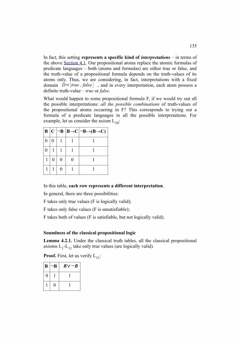
135

In fact, this setting represents a specific kind of interpretations – in terms ofthe above Section 4.1. Our propositional atoms replace the atomic formulas ofpredicate languages – both (atoms and formulas) are either true or false, andthe truth-value of a propositional formula depends on the truth-values of itsatoms only. Thus, we are considering, in fact, interpretations with a fixeddomain D={true , false } , and in every interpretation, each atom possess adefinite truth-value – true or false.

What would happen to some propositional formula F, if we would try out allthe possible interpretations: all the possible combinations of truth-values ofthe propositional atoms occurring in F? This corresponds to trying out aformula of a predicate languages in all the possible interpretations. Forexample, let us consider the axiom L10:

B C ¬B B→C ¬B→(B→C)

0 0 1 1 1

0 1 1 1 1

1 0 0 0 1

1 1 0 1 1

In this table, each row represents a different interpretation.

In general, there are three possibilities:

F takes only true values (F is logically valid);

F takes only false values (F is unsatisfiable);

F takes both of values (F is satisfiable, but not logically valid).

Soundness of the classical propositional logic

Lemma 4.2.1. Under the classical truth tables, all the classical propositionalaxioms L1-L11 take only true values (are logically valid).

Proof. First, let us verify L11:

B ¬B B∨¬ B

0 1 1

1 0 1

136

And L10 is, in fact, verified in the table above.

Exercise 4.2.1. Verify that the axioms L1-L9 take only true values as well.

Q.E.D.

See also:"Truth Tables" from The Wolfram Demonstrations Project. Contributed by Hector Zenil.

Lemma 4.2.2. If, under the classical truth tables, the formulas B and B→Ctake only true values, then so does C. I. e. from "always true" formulas, ModusPonens allows deriving only of "always true" formulas.

Proof. Let us assume that, in some interpretation, C takes a false value. In thesame interpretation, B and B→C take true values. If B is true, and C is false,then B→C is false. Contradiction. Hence, C takes only true values. Q.E.D.

Note. In the proof of Lemma 4.2.2, only the third row of implication truthtable was significant: if B is true, and C is false, then B→C is false!

Theorem 4.2.3 (soundness of the classical propositional logic).

If [L1-L11, MP]:├ F, then, under the classical truth tables, F takes only true

values (is logically valid).

Proof. By induction, from Lemmas 4.2.1 and 4.2.2.

In particular: the classical propositional logic is consistent – in the sense thatone cannot prove both [L1-L11, MP]:├ G and [L1-L11, MP]:├ ¬G , for

any formula G. Indeed, a formula and its negation cannot both be true.

Completeness of classical propositional logic

How about the converse statement of Theorem 4.2.3: if, under the classicaltruth tables, formula F takes only true values, then [L1-L11, MP]:├ F? Is our

system powerful enough to prove any formula that is taking only truevalues? The answer is "yes":

Theorem 4.2.4 (completeness of the classical propositional logic). Assume,the formula F has been built of the formulas B1, B2, ..., Bn by using

propositional connectives only. If, under the classical truth tables, for anytruth-values of B1, B2, ..., Bn, formula F takes only true values, then:

a) in the constructive logic,

[L1-L10, MP]: B1∨¬ B1 , B2∨¬ B2 , ... , Bn∨¬ Bn ├ F,

b) in the classical logic, [L1-L11, MP]:├ F.

137

Of course, (b) follows from (a) immediately − all the premisesB1∨¬ B1 , B2∨¬ B2 , ... , Bn∨¬ Bn are instances of the axiom L11.

Corollary 4.2.4. The classical propositional logic [L1-L11, MP] is "complete"

also in the sense that if one would add any formula that can't be proved in thislogic, then one would obtain a system, in which all formulas are provable, i.e.,an inconsistent system.

Proof of the corollary. Indeed, according to the soundness theorem, if someformula F cannot be proved in [L1-L11, MP], then it takes false value for some

combination of truth-values of its atoms. Replace each true atom by theformula A→A, and each false atom – by ¬(A→A). In this way we obtain aformula F' that takes only false values, hence, ¬F' takes only true values, andhence, according to the completeness theorem, it can be proved in [L1-L11,

MP]. Thus, if we would add F to [L1-L11, MP] as an axiom schema, then, in

this system, the formulas F' and ¬F' will be provable, and by L10 – any

formula will be provable. Q.E.D.

Note. Assume, the formula F is built of atoms B1, B2, ..., Bn by using

propositional connectives only. If, under the classical truth tables, for any(possible and impossible) truth-values of B1, B2, ..., Bn, formula F takes only

true values, then F is called a tautology. Thus, Theorem 4.2.4 says that anytautology can be proved in the classical propositional logic.

Completeness of the classical propositional logic was first proved by Emil L.Post in his 1920 Ph.D. thesis, and published as

E. Post. Introduction to a general theory of elementary propositions. American Journal ofMathematics, 1921, vol. 43, pp.163-185.

About the history, see also:

Richard Zach. Completeness before Post: Bernays, Hilbert, and the development ofpropositional logic. The Bulletin of Symbolic Logic, 1999, vol. 5, N3, pp.331-366.

Now, let us prove Theorem 4.2.2. Following an elegant later idea by LaszloKalmar we need two simple lemmas before trying to prove the theorem.

L. Kalmar. Über Axiomatisiebarkeit des Aussagenkalküls. Acta scientiariummathematicarum (Szeged). 1934-35. vol. 7, pp. 222-243.

Lemma 4.2.5. In the constructive logic, one can "compute" the classical truth-values of ¬ B , B →C , B∧C , B∨C as in the Table 4.1.

Note. Thus, to "compute" the classical truth-values, the axiom L11 is not

necessary!

Proof.

138

¬B ├ ¬B

Immediately, in any logic.

B ├ ¬ ¬B

By Theorem 2.4.4. [L1, L2, L9, MP]: A→¬¬A.

¬B, C ├ B→C

¬B, ¬C ├ B→C

By axiom L10: ¬B→(B→C) we obtain ¬B ├ B→C. This covers both cases.

B, ¬C ├ ¬(B→C)

This is exactly Theorem 2.4.2(a) [L1, L2, L9, MP].

B, C ├ B→C

By axiom L1: C→(B→C) we obtain C ├ B→C.

Table 4.1.

Negation Implication Conjunction Disjunction

[ ]:

¬B ├ ¬B

[L10, MP]:

¬B, ¬C ├ B→C

[L1, L2, L3, L9, MP]:

¬B, ¬C ├¬(B∧C )

[L1-L4, L8, L9,

MP]: ¬B,¬C ├¬(B∨C )

[L1, L2, L9,

MP]:

B ├ ¬¬B

[L10, MP]:

¬B, C ├ B→C

[L1, L2, L3, L9, MP]:

¬B, C ├ ¬(B∧C )

[L7, MP]:

¬B, C ├ B∨C

[L1, L2, L9, MP]:

B, ¬C ├ ¬(B→C)

[L1, L2, L4, L9, MP]:

B, ¬C ├ ¬(B∧C )

[L6, MP]:

B, ¬C ├ B∨C

[L1, MP]:

B, C ├ B→C

[L5, MP]:

B, C ├ B∧C

[L6, MP]:

B, C ├ B∨C

¬B, ¬C ├ ¬(B∧C )

¬B, C ├ ¬(B∧C )

By axiom L3: B∧C → B and the Contraposition Law [L1, L2, L9, MP]:

(A→B)→(¬B→¬A) we obtain ¬ B →¬(B∧C) , and ¬B ├

139

¬(B∧C ) . This covers both cases.

B, ¬C ├ ¬(B∧C )

By axiom L4: B∧C → C and the Contraposition Law [L1, L2, L9, MP]:

(A→B)→(¬B→¬A) we obtain ¬C → ¬(B∧C ) , and ¬C ├ ¬(B∧C ) .

B, C ├ B∧C

By axiom L5: B →(C → B∧C ) we obtain B, C ├ B∧C .

¬B, ¬C ├ ¬ (B∨C )

The most complicated case. By de Morgan Laws, in the minimal logic:¬B∧¬C →¬(B∧C ) . You may wish to verify that even less – [L1-L4, L8,

L9, MP] is sufficient.

¬B, C ├ B∨C

By axiom L7: C → B∨C we obtain C ├ B∨C .

B, ¬C ├ B∨C ; B, C ├ B∨C

By axiom L6: B → B∨C we obtain B ├ B∨C . This covers both cases.

Q.E.D.

As the next step, let us generalize Lemma 4.2.5 by showing how to "compute"truth-values of arbitrary formula F, which is built of formulas B1, B2, ..., Bn by

using more than one propositional connective. For example, let us take theformula B∨C → B∧C :

B C B∨C B∧C B∨C → B∧C

0 0 0 0 1

0 1 1 0 0

1 0 1 0 0

1 1 1 1 1

We will show that, in the constructive logic [L1-L10, MP]:

¬B, ¬C ├ B∨C → B∧C ,¬B, C ├ ¬(B∨C → B∧C) ,

B, ¬C ├ ¬(B∨C → B∧C) ,

¬B, ¬C ├ B∨C → B∧C .

140

Lemma 4.2.6. Assume, the formula F has been built of the formulas B1,

B2, ..., Bn by using propositional connectives only. Assume that, if the

formulas B1, B2, ..., Bn take the truth-values v1, v2, ..., vn respectively, then,

for these values, formula F takes the truth-value w. Then, in the constructivelogic, we can "compute" the truth-value of F in the following sense:

[L1-L10, MP]: v1B1, v2B2, ..., vnBn├ wF,

where: wF denotes F, if w is true, and ¬F, if w is false, and viBi denotes Bi, if

vi is true, and ¬Bi, if vi is false.

Proof. By induction.

Induction base. F is one of the formulas Bi. Then w=vi, and, of course, in any

logic, viBi├ wF.

Induction step.

Note that Lemma 4.2.5 represents the assertion of Lemma 4.2.6 for formulasbuilt of B1, B2, ..., Bn by using a single propositional connective.

1. F is ¬G. By the induction assumption,

[L1-L10, MP]: v1B1, v2B2, ..., vnBn├ w'G,

where w' represents the truth-value of G. By Lemma 4.2.5,

[L1-L10, MP]: w'G├ wF, hence, [L1-L10, MP]: v1B1, v2B2, ..., vnBn├ wF.

2. F is GoH, where o is implication, conjunction, or disjunction. By theinduction assumption,

[L1-L10, MP]: v1B1, v2B2, ..., vnBn├ w'G,

where w' represents the truth-value of G, and

[L1-L10, MP]: v1B1, v2B2, ..., vnBn├ w''H,

where w'' represents the truth-value of H. By Lemma 4.2.5,

[L1-L10, MP]: w'G, w''H├ wF,

hence, [L1-L10, MP]: v1B1, v2B2, ..., vnBn├ wF.

Q.E.D.

Proof of Theorem 4.2.4(a). By Lemma 4.2.6:

[L1-L10, MP]: B1, v2B2, ..., vnBn├ F,

[L1-L10, MP]: ¬B1, v2B2, ..., vnBn├ F,

141

because F takes only true values. Then, by [L1, L2, L8, MP] D-elimination

theorem:

[L1-L10, MP]: B1v¬B1, v2B2, ..., vnBn├ F.

By repeating this operation we obtain Theorem 4.2.4(a):

[L1-L10, MP]: B1∨¬ B1 , B2∨¬ B2 , ... , Bn∨¬ Bn ├ F.

Q.E.D.

The above proof of the Completeness Theorem contains, in fact, an algorithmallowing to build a (very long) proof of any propositional formula that takesonly true values.

Computational complexity of the problem

From now on, in principle, we could forget our great ability of provingformulas in the classical propositional logic that we developed in Section 2.Indeed, in order to verify, is a formula provable in [L1-L11, MP], or not, we

can simply check, under the classical truth tables, takes this formula only truevalues, or not. If it takes, then, by the Completeness Theorem, formula isprovable, if not – it is not provable.

For example, instead of trying to prove Peirce’s Law a la Section 2, we cansimply verify that it takes only true values:

A B A→ B (A→ B)→ A (( A→ B)→ A)→ A

0 0 1 0 1

0 1 1 0 1

1 0 0 1 1

1 1 1 1 1

Thus, by Theorem 4.2.4 (completeness of the classical propositional logic),

[L1-L11, MP]: (( A→ B)→ A)→ A .

For formulas containing one, two or three atoms, this method is really simplerthan direct proving of formulas in [L1-L11, MP]. However, for longer

formulas, this method allows for building automatically (by using Lemmas4.2.5 and 4.2.6) only of extremely long proofs.

Indeed, if the formula F contains n different atoms A, B, C, ..., then its truth

142

table contains 2n rows for which the truth values of F must be checked oneby one. Of course, if the formula contains 2 atoms (like as Peirce’s Law, or 3atoms (like as the Axiom L2), then its truth table consists of 4 or 8 rows − for

most people this is a feasible task. But the truth table for a formula containing100 atoms contains 2100≈1030 rows to check!

So, let us try inventing a more efficient algorithm? Unfortunately, until now,all the attempts have produced only algorithms the running time of which (forchecking of formulas of length n, as n→∞ ), exceeds any power nk .

And it seems, we will never really succeed, because of the Cook-LevinTheorem proved in 1971.

Cook-Levin Theorem. The problem of determining, is a propositionalformula satisfiable, or not, belongs to the complexity class NP-complete.

For details, see Cook-Levin Theorem, Stephen Co ok and Leonid Levin in Wikipedia.

Corollary. The problem of determining, is a propositional formula provablein the classical propositional logic, or not, belongs to the complexity classco-NP-complete.

Indeed, a propositional formula is provable in the classical propositional logicif and only if it takes only true values.

It is believed that the running time of any algorithm solving problems of thesetwo classes (for checking of formulas of length n, as n→∞ ), exceeds anypower nk . It is believed, but not yet proved (see P versus NP problem inWikipedia) – it is one of the “major unsolved problems in computer science”.

The problem of determining the constructive provability of propositionalformulas is believed to be even harder – it belongs to the complexity classP SPACE-complete , as proved by Richard Statman in 1979:

R. Statman. Intuitionistic propositional logic is polynomial-space complete, TheoreticalComputer Science 9 (1979), pp. 67–72 (online copy available).

It is believed that PSPACE-complete problems are strictly harder than co-NP-complete problems.

Worst case estimates and practical experience

When trying to assess the performance of some algorithm, for example, of analgorithm A, which is determining correctly the provability of formulas, wecan start by considering of some abstract functions, such as:

TIME A(F ) – the time that A is spending to process the formula F,

SPACE A(F ) – the memory space that A is using to process F.

143

Then, the “overall performance” of A can be estimated as follows:

maxTIME A(n) – the time that A is spending to process the “worst” of the formulas having length n;

maxSPACE A(n) – similarly, for the memory space.

For example, when analyzing the simplest algorithms, that are determiningcorrectly the provability of formulas in the classical propositional logic, onecan verify easily that

maxTIME A(n)=2Cn ,

where C is a numerical constant (the less constant, the better the algorithm).

However, this does not imply that all such algorithms are useless in solving ofpractical problems. The above estimate represents the so-called worst caseestimate: there exist, indeed, formulas of length n, the processing time ofwhich by the algorithm is unacceptable. But how about the majority offormulas? Or, about specific types of formulas appearing when solving aspecific practical problem? Experience shows that some of the universalalgorithms showing unacceptable worst case results, perform really good inmany practical cases. For examples, see the tableaux method and theresolution method considered in Section 6 and Section 7.

4.3. Classical Predicate Logic − Gödel's Completeness Theorem

Kurt Gödel (1906-1978) "He is best known for his proof of Gödel's Incompleteness Theorems.In 1931 he published these results in Über formal unentscheidbare Sätze der PrincipiaMathematica und verwandter Systeme . ...Gödel's results were a landmark in 20th-centurymathematics, showing that mathematics is not a finished object, as had been believed. It alsoimplies that a computer can never be programmed to answer all mathematical questions."(According to MacTutor History of Mathematics archive).

As David Hilbert and Wilhelm Ackermann published in

D. Hilbert, W. Ackermann. Grundzüge der theoretischen Logik. Berlin (Springer), 1928

their, in a sense, "final" version of the axioms of classical logic, they noted:"Whether the system of axioms is complete at least in the sense that all thelogical formulas which are correct for each domain of individuals can actuallybe derived from them, is still an unsolved question."

(quoted afterS. C. Kleene. The Work of Kurt Gödel. "The Journal of Symbolic Logic", December 1976, Vol.41, N4, pp.761-778See also: Hilbert and Ackermann's 1928 Logic Book by Stanley N. Burris).

144

Indeed, as we will verify below,

a) all axioms of the classical logic (L1-L15) are logically valid,

b) the inference rules MP, Gen, from logically valid formulas, infer onlylogically valid formulas.

Hence, in the classical logic, only logically valid formulas can be proved(soundness theorem). Still, is our list of logical axioms and rules of inferencecomplete in the sense that all logically valid formulas can be proved? − thequestion asked by Hilbert and Ackermann in 1928. The answer is "yes" − asKurt Gödel established in 1929, in his doctoral dissertation "Über dieVollständigkeit des Logikkalküls" (visit Gödel's archive at the PrincetonUniversity Library). The corresponding paper was published in 1930:

K. Gödel. Die Vollständigkeit der Axiome des logischen Funktionenkalküls. "Monatsheftefuer Mathematik und Physik", 1930, Vol.37, pp.349-360.

Theorem 4.3.1 (Gödel's Completeness Theorem). In any predicate language,if a formula is logically valid, then it can be proved by using the classical logic[L1-L15, MP, Gen].

In fact, a more general theorem can be proved:

Theorem 4.3.2 (Thanks to Sune Foldager for the idea.). If T is a first ordertheory with classical logic, then, if some formula F is true in all models of T,then T proves F.

Thus (as noted in Section 1.3), in principle, we will never need to introducespecific (non-logical) rules of inference. All the consequences of the axioms ofa first order theory can be derived by using our logical axioms and two rules ofinference – Modus Ponens and Generalization.

Gödel's Completeness Theorem follows from Theorem 4.3.2 (simply considera theory T with an empty set of specific axioms).

Soundness of the classical predicate logic

First, let us prove the Soundness Theorem − that all the formulas that can beproved by using the classical logic [L1-L15, MP, Gen] are logically valid.

Lemma 4.3.1. All the axioms of the classical logic (L1-L15) are logically

valid.

Proof.

1) Under the classical truth tables, the propositional axioms L1-L11 take only

true values (Lemma 4.2.1). Hence, these axioms are true under allinterpretations.

145

2a) L12: xF(x)→F(t), where F is any formula, and t is a term such that the∀substitution F(x/t) is admissible.

We proved the logical validity of this axiom in Section 4.1.

2b) L13: F(t)→ xF(x), where F is any formula, and t is a term such that the∃z(x+z+1=y).substitution F(x/t) is admissible.

Similarly, do Exercise 4.3.1.

2c) L14: x(G→F(x))→(G→ xF(x)), where F is any formula, and G is a∀ ∀formula that does not contain x as a free variable.

Let us assume that, under some interpretation J, for some values of its freevariables, L14 is false. According to the classical truth tables, this could be

only, if x(G→F(x)) were true, and G→ xF(x) were false (under the∀ ∀interpretation J, for the same above-mentioned values of free variables)

If x(G→F(x)) is true, then G→F(c) is true for all∀ c∈D J . Since G does notcontain x, this means that if G is true, then F(c) is true for all c∈DJ .

On the other hand, if G→ xF(x) is false, then G is true, and xF(x) is false.∀ ∀And finally, if xF(x) is false, then F(c) is false for some∀ c∈DJ . But, as weestablished above, if G is true, then F(c) is true for all c∈DJ . Contradiction.Hence, under all interpretations, L14 is true for all combinations of its free

variables.

2d) L15: x(F(x)→G)→( xF(x)→G), where F is any formula, and G is a∀ ∃z(x+z+1=y).formula that does not contain x as a free variable.

Similarly, do Exercise 4.3.1.

Q.E.D.

Exercise 4.3.1. Verify that the axioms L13 and L15 are logically valid as well.

Lemma 4.3.2. a) For any interpretation J, from formulas true under J, theinference rules MP and Gen allow deriving only of formulas true under J.

b) From logically valid formulas, the inference rules MP and Gen allowderiving only of logically valid formulas.

Proof. Of course, (b) follows from (a). Let us prove (a).

1. Modus Ponens. Assume, B and B→C are true under J. By MP, we derive C.Assume, C is false under J, for some values of its free variables. For thesevalues of the free variables of C, the formulas B and B→C are true under J.Then, according to the classical truth tables, C also must be true.Contradiction. Hence, C is true under J.

146

2. Generalization. Assume, F(x) is true under J, but xF(x) is false under J,∀for some values of its free variables. Hence, under J, for these values of freevariables of xF(x), there is∀ c∈DJ such that F(c) is false. But F(x) is trueunder J, i.e., F(c) is true as well. Contradiction. Hence, xF(x) is true under J.∀

Q.E.D.

Theorem 4.3.3 (soundness of the classical predicate logic). All the formulasthat can be proved by using the classical logic [L1-L15, MP, Gen], are logically

valid.

Proof. Immediately, by Lemmas 4.3.1 and 4.3.2(b).

Corollary 4.3.3. If T is a first order theory with the classical logic, the specificaxioms of which are true under some interpretation J, then:

a) All theorems of T are true under J as well. In other words, theorems of Tare true in any model of T.

b) T is consistent (i.e., it does not prove contradictions).

Proof. a) In T, each proof consists of instances of logical axioms (true underany interpretation, Lemma 4.3.1), of instances of specific axioms of T (trueunder J), and of formulas that can be obtained from these by (repeated)application of MP and Gen. By Lemma 4.3.2(a), the latter are true under J aswell.

b) Assume, T proves a contradiction – some formula B and simultaneously –¬B . Then, by (a) these formulas both are true under J. This is impossible.

Q.E.D.

Completeness of the classical predicate logic

The following 12 pages present a proof of Gödel's Completeness Theorem.

Model Existence Theorem

Gödel's Completeness Theorem (and Theorem 4.3.2) are easy consequences ofthe so-called Model Existence Theorem (see below), first proved in the above-mentioned Gödel's paper of 1930.

Gödel's initial proof was simplified in 1947, when Leon Henkin presented inhis Ph.D. thesis a new proof of the Model Existence Theorem. The result waspublished in 1949:

L. Henkin. The completeness of the first-order functional calculus. "J. Symbolic Logic",1949, vol.14, pp.159-166.

147

See also Henkin's later account of his discovery:

L. Henkin. The discovery of my completeness proofs. "The Bulletin of Symbolic Logic",1996, vol.2, N2, pp.127-158.

An even simpler version Henkin's proof was found independently and almostsimultaneously by Gisbert Hasenjäger (during WWII, “was responsible for thesecurity of the Enigma machine”). However, when publishing, Hasenjägeracknowledged Henkin's priority:

G. Hasenjäger. Eine Bemerkung zu Henkin's Beweis für die Vollständigkeit desPrädikatenkalküls der ersten Stufe. "J. Symbolic Logic", 1953, vol.18, pp.42-48.

If T is an inconsistent theory, then there are no models of T. Indeed, if T provesa contradiction, i.e., a formula of the kind B∧¬B , then, in a model of T, theformula B must be true and false simultaneously. This is impossible.

Hence, if there is a model of T, then T is consistent.

The converse question: could it be possible that T is a consistent theory, butthere are no models of T? The answer is given in the

Theorem 4.3.4 (Model Existence Theorem). If a first order formal theorywith classical logic is consistent (in the sense that, by using the classical logic,it does not prove contradictions), then there is a finite or countable model ofthis theory (an interpretation with a finite or countable domain, under whichall axioms and theorems of theory are true).

In the 1920s, some people insisted that mere consistency of a theory (in thesyntactic sense of the word − as the lack of contradictions) is not sufficient toregard it as a meaningful theory − as a "theory of something". ModelExistence Theorem says the contrary − (syntactic!) consistency of a theory issufficient: if a theory does not contain contradictions, then it is a "theoryof something" − it describes at least some kind of "mathematical reality". Forexample, you may think that Euclidean geometry is "meaningless" − because itdoes not describe 100% correctly the spacial properties of the Universe. Butit's your problem, not Euclid's − use another theory, if necessary. Euclideangeometry describes its own kind of "mathematical reality" – and 100%correctly!

Let us assume the Model Existence Theorem (we will prove it later in thisSection).

Proof of Theorem 4.3.2.

If T proves F, then F is true in all models of T (Corollary 4.3.3).

Now, let us assume that some formula F is true in all models of theory T (forall values of its free variables, if any), yet it cannot be proved in T. Let us

148

consider the theory T' in the language of T which contains (besides the axiomsof T) an additional non-logical axiom − the negation of F, i.e., the formula¬ x∀ 1... x∀ nF, where x1, .., xn are exactly all the free variables appearing in F

(if F contains free variables x1, .., xn, then, to negate its assertion, we must add

the quantifiers x∀ 1... x∀ n). Since F cannot be proved from the axioms of T, T'

is a consistent theory.

Indeed, if T' would be inconsistent, i.e., we could prove in T' some formula Cand its negation ¬C, then we had proofs of [T]: ¬ x∀ 1... x∀ nF├ C, and [T]:

¬ x∀ 1... x∀ nF├ ¬C. Since ¬ x∀ 1... x∀ nF is a closed formula, by Deduction

Theorem 2, [T]:├ ¬ x∀ 1... x∀ nF →C, and [T]:├ ¬ x∀ 1... x∀ nF →¬C. Now, by

axiom L9: (B→C)→(B→¬C)→¬B, we obtain that [T]:├ ¬¬ x∀ 1... x∀ nF. By

the (classical) Double Negation Law, this implies [T]:├ x∀ 1... x∀ nF, and by

axiom L12: xB(x)→B(x) we obtain [T]:├ F. But, by our assumption, F∀cannot be proved in T. Hence, T' is a consistent theory, indeed.

Now, by the Model Existence Theorem, there is a model of T' – aninterpretation J that makes all its axioms true. Under this interpretation, allaxioms of T are true, thus, J is a model of T. And the formula ¬ x∀ 1... x∀ nF (as

an axiom of T') is true under J as well. On the other hand, since F is true in allmodels of T, it is true also under the interpretation J. Hence, formulas

x∀ 1... x∀ nF and ¬ x∀ 1... x∀ nF both are true under J. This is impossible, hence,

F must be provable in T. Q.E.D.

Notes. a) Such a simple proof seems almost impossible! We are proving thatthe logical axioms and rules of inference are strong enough to prove all theformulas that are true in all models of T, but where come these axioms in?They come in − in the proof of the Model Existence Theorem. This theoremsays that if some formal theory T does not have models, then the logicalaxioms and rules of inference are strong enough to derive a contradiction fromthe axioms of T. But the proof of the Model Existence Theorem that we willconsider below, is positive, not negative!

b) The above simple proof seems to be extremely non-constructive! "If F istrue in all models of T, then it can be proved in T". How could we obtain thisproof? Still, how do we know that F is true in all models of T? Only, if we hada constructive procedure that is verifying this, we could ask for an algorithmconverting such procedures into proofs in T!

Exercise 4.3.2 (optional, for smart students). Prove the Model ExistenceTheorem by using the following smart ideas due to Gödel, Henkin andHasenjäger. Let T be a consistent theory. We must build a model of T. Whatkind of "bricks" could we use for this "building"? Idea #1: let us use object

149

constants of the language! So, let us add to the language of T an infinite set ofnew object constants d1, d2, d3, ... (and adopt the corresponding additional

instances of logical axioms). Prove that this extended theory T0 is consistent.

The model we are building must contain all "objects" whose existence can beproved in T0. Idea #2: for each formula F of T0 having exactly one free

variable (for example, x) let us add to the theory T0 the axiom xF(x)→F(d∃z(x+z+1=y). i),

where the constant di is unique for each F. If T0 proves xF(x), then this∃z(x+z+1=y).constant di will represent in our model the object x having the property F.

Prove that this extended theory T1 is consistent. Idea #3: prove the (non-

constructive) Lindenbaum's Lemma: the axiom set of any consistent theorycan be extended in such a way, that the extended theory is consistent andcomplete (the axiom set of this extended theory may be not algorithmicallysolvable, let us allow this). By using this lemma, extend T1 to a consistent

complete theory T2. Idea #4: let us start building of a model M of T by taking

as the domain of M the set of all those terms of T0 that do not contain

variables. And let us interpret each function constant f as the "syntacticconstructor function" f', i.e., let us define the value f'(t1, ..., tn) simply as the

character string "f(t1, ..., tn)". Finally, let us interpret each predicate constant p

as a (non-constructive) relation p' such that p'(t1, ..., tn) is true in M if and only

if T2 proves p'(t1, ..., tn). To complete the proof, prove that an arbitrary formula

G is true in M if and only if T2 proves G. Hence, all theorems of the initial

theory T are true in M.

Adolf Lindenbaum (1904-1941), his wife Janina Hosiasson-Lindenbaum (1899-1942).

Lemma 4.3.4 (Lindenbaum's Lemma). Any consistent first order theory canbe extended to a consistent complete theory. More precisely, if T is aconsistent first order theory, then, in the language of T, there is a set A ofclosed formulas such that T+A is a consistent complete theory.

Note. a) By T+A we denote the first order theory in the language of T,obtained from T by adding the formulas of the set A as non-logical axioms.

b) In general, T+A is not a formal theory in the sense of Section 1.1 – the set Anot always is algoritmically solvable.

Exercise 4.3.3. Verify that, in any predicate language L, only countably manyformulas can be generated: produce an algorithm for printing out a sequenceF0, F1, F2, ... containing all the formulas of L.

Proof of Lindenbaum's Lemma (Attention: non-constructive reasoning!)

150

Let us use the algorithm of the Exercise 4.3.3 printing out the sequence F0, F1,

F2, ... of all formulas in the language of T, and let us run through this

sequence, processing only those formulas Fi that are closed.

At the very beginning, the set of new axioms A0 is empty.

At the step i, we already have some set Ai-1 of new axioms. If the formula Fi is

not closed, let us ignore it, and set Ai=Ai-1. Now, let us suppose that Fi is a

closed formula. If T+Ai-1 proves Fi, or T+Ai-1 proves ¬Fi, then we can ignore

this formula, and set Ai=Ai-1. If T+A does not prove neither Fi, nor ¬Fi, then

let us simply add Fi (or ¬Fi, if you like it better) to our set of new axioms, i.e.,

set Ai=Ai−1∪{F i} .

Etc., ad infinitum. As the result of this process we obtain a set of closedformulas A=A0∪A1∪A2∪...∪Ai∪ ... .

Let us prove that T+A is a consistent complete theory.

Consistency. If T+A would be inconsistent, we would have a proof of [T+A]:C∧¬C for some formula C. If, in this proof, no axioms from the set A

would be used, we would have a proof of [T]: C∧¬C , i.e., T would beinconsistent.

Otherwise, the proof of [T+A]: C∧¬C contains a finite number of axiomsB1, ..., Bk from the set A. Let us arrange these axioms in the sequence, as we

added them to the set A. Thus we have a proof of [T]: B1, ..., Bk├ C∧¬C .

Then, by the N-elimination theorem, we have a proof of [T]: B1, ..., Bk-1├

¬Bk. But this is impossible − we added Bk to the set A just because T+Ai-1

could not prove neither Bk, nor ¬Bk. Q.E.D.

Completeness. We must verify that, for any closed formula F in the languageof T, either T+A├ F, or T+A├ ¬F. Let us assume, this is not the case for someclosed formula F. Of course, F appears in the above sequence F0, F1, F2, ... as

some Fi. If neither T+A├ F, nor T+A├ ¬F, then neither T+Ai-1├ Fi, nor

T+Ai-1├ ¬Fi. In such a situation we would add F or ¬F to the set A, hence, we

would have T+A├ F or T+A├ ¬F. Q.E.D.

This completes the proof of Lindenbaum's Lemma.

Attention: non-constructive reasoning! T+A is a somewhat strange theory,because, in general, we do not have an algorithmic decision procedure for itsset of axioms. Indeed, to decide, is some closed formula F an axiom of T+A,or not, we must identify F in the sequence F0, F1, F2, ... as some Fi, and after

151

this, we must verify, whether T+Ai-1 proves Fi, or T+Ai-1 proves ¬Fi, or none

of these. Thus, in general, T+A is not a formal theory in the sense of Section1.1.

Proof of the Model Existence Theorem

(Attention: non-constructive reasoning!)

Inspired by the beautiful exposition in Mendelson [1997].

Step 1. We must build a model of T. What kind of "bricks" should we use forthis "building"? Idea #1: let us use object constants of the language! So, inorder to prepare enough "bricks", let us add to the language of T a countableset of new object constants d1, d2, d3, ... (and extend the definitions of terms,

atomic formulas and formulas accordingly, and add new instances of logicalaxioms accordingly). Let us prove that, if T is consistent, then this extendedtheory T0 also is consistent.

If T0 would be inconsistent, then, for some formula C, we could obtain a proof

of [T0]: C∧¬C . If, in this proof, object constants from the set {d1, d2,

d3, ...} would not appear at all, then, in fact, we had a proof of [T]: C∧¬C ,

i.e., we could conclude that T is inconsistent. But what, if some of the newobject constants do appear in the proof of [T0]: C∧¬C ? Then, let us

replace these constants by any variables of T that do not appear in this proof(this is possible, since each predicate language contains a countable set ofobject variables). After these substitutions, the proof becomes a valid proof ofT, because:

a) The logical axioms remain valid.

b) The non-logical axioms of T do not contain the object constants d1, d2,

d3, ..., so, they do not change.

c) Applications of inference rules MP and Gen remain valid.

Hence, [T]: C ' ∧¬C ' , where the formula C' has been obtained from C bythe above substitutions. Thus, if T0 would be inconsistent, then so would be T.

Step 2. The model we are building must contain all "objects" whose existencecan be proved in T0. Idea #2: for each formula F of T0 having exactly one free

variable (for example, x) let us add to the theory T0 the axiom xF(x)→F(d∃z(x+z+1=y). i),

where the constant di is unique for each F. If T0 proves xF(x), then this d∃z(x+z+1=y). i

will represent in our model the object x having the property F. Let us provethat, if T is consistent, then this extended theory T1 also is consistent. Note that

152

in T1 the same language is used as in T0.

To implement the Idea #2 correctly, first let us use the algorithm of theExercise 4.3.3 printing out the sequence F0, F1, F2, ... of all formulas in the

language of T0, and let us run through this sequence, processing only those

formulas Fi that have exactly one free variable. Let us assign to each such

formula Fi a unique constant dc(i) in such a way that dc(i) does not appear

neither in the non-logical axioms of T, nor in Fi, nor in the axioms

yF∃z(x+z+1=y). j(y)→Fj(dc(j)) for all formulas Fj preceding Fi in the sequence F0, F1,

F2, .... And, if x is the (only) free variable of Fi, let us adopt xF∃z(x+z+1=y). i(x)→Fi(dc(i))

as an axiom of T1.

Now, let us assume that the extended theory T1 is inconsistent, i.e., that, for

some formula C in the language of T0, we have a proof of [T1]: C∧¬C . In

this proof, only a finite number n of axioms xF∃z(x+z+1=y). i(x)→Fi(dc(i)) could be used.

Let us arrange these n axioms in order of increasing indices i, and let us denotethis list by A1, A2, ..., An.

If n=0, then we have [T0]: C∧¬C , i.e., then T0 is inconsistent. This is

impossible.

If n>0, then let us consider An – the last axiom of the list: xF(x)→F(d∃z(x+z+1=y). c(F)).

And, in the proof of [T1]: C∧¬C , let us replace the constant d c(F ) by

some variable y that does not appear in this proof (this is possible, since eachpredicate language contains a countable set of variables). After thissubstitution, the proof remains a valid proof of T1, because:

a) The logical axioms remain valid.

b) The non-logical axioms of T do not contain the constant c(F), they do notchange.

c) The axiom xF(x)→F(d∃z(x+z+1=y). c(F)) becomes xF(x)→F(y). Since F does not∃z(x+z+1=y).contain the constant c(F), the premise xF(x) does not change.∃z(x+z+1=y).

d) The remaining n-1 axioms yF∃z(x+z+1=y). j(y)→Fj(dc(j)) of T1 , i.e., the formulas of the

list A1, A2, ..., An-1 do not contain the constant d c(F ) , they do not change.

e) Applications of inference rules MP and Gen remain valid.

Thus we have now a new proof of a contradiction:

[T0]: A1, A2, ..., An-1, xF(x)→F(y)├∃z(x+z+1=y). C '∧¬C ' ,

153

where the formula C' has been obtained from C by substituting y for d c(F ) .Then, by N-elimination theorem, there is a proof:

[T0]: A1, A2, ..., An-1├ ¬( xF(x)→F(y)).∃z(x+z+1=y).

By Theorem 2.6.5, [L1-L11, MP]: ¬(A→ B)→ A∧¬B . Thus, from

¬( xF(x)→F(y)) we can conclude∃z(x+z+1=y). ∃z(x+z+1=y). x F (x )∧¬F ( y) , and we have a proofof xF(x), and a proof of ¬F(y). By applying Gen to the second formula, we∃z(x+z+1=y).obtain y¬F(y), that is equivalent to ¬ yF(y) (indeed, let us remind ∀ ∃z(x+z+1=y). Section3.2, Table 3.2, Group IV, constructively, x¬B↔¬ xB). By Replacement∀ ∃z(x+z+1=y).Theorem 3, ¬ yF(y) is equivalent to ¬ xF(x). Thus, we have a proof of a∃z(x+z+1=y). ∃z(x+z+1=y).contradiction ∃z(x+z+1=y). x F (x )∧¬∃z(x+z+1=y). x F (x) , where only the axioms [T0]: A1, A2, ...,

An-1 are used.

Let us repeat the above chain of reasoning another n−1 times to eliminateall occurrences of the axioms xF∃z(x+z+1=y). i(x)→F(dc(i)) from our proof of a

contradiction. In this way we obtain a proof of a contradiction in T0. This is

impossible. Hence, T1 is a consistent theory.

Step 3. Idea #3: let us use the (non-constructive!) Lindenbaum's Lemma, andextend T1 to a consistent complete theory T2. Note that in T2 the same

language is used as in T0.

Step 4. Let us define an interpretation M of the language of T0, in which all

theorems of T2 will be true. Since all theorems of the initial theory T are

theorems of T2, this will complete our proof.

Idea #4: let us take as the domain DM of the interpretation M the (countable!

− verify!) set of all constant terms of T0, i.e., terms that do not contain

variables (this set of terms is not empty, it contains at least the countable set ofobject constants added in Step 1). And let us define interpretations of objectconstants, function constants and predicate constants as follows.

a) The interpretation of each object constant c is the constant c itself.

b) The interpretation of a function constant f is the "syntactic constructorfunction" f’’, i.e., if f is an n-ary function constant, and t1, ..., tn are constant

terms, then the value f”(t1, ..., tn) is defined simply as the character string "f(t1,

..., tn)" (quotation marks ignored).

c) The interpretation of a predicate constant p is the relation p” such, if p is ann-ary predicate constant, and t1, ..., tn are constant terms, then p”(t1, ..., tn) is

154

defined as true in M if and only if T2 proves p(t1, ..., tn) (note that T2 is a

consistent complete theory, it proves either p(t1, ..., tn), or ¬p(t1, ..., tn), but not

both!).

Step 5. To complete the proof, we must verify that, in the language of T0, an

arbitrary formula G is true in M if and only if T2 proves G (let us denote this,

as usual, by T2├ G). This will be done, if we will prove that, if x1, ..., xm is

any list of variables, containing all the free variables contained in the formulaG, and t1, ..., tm are constant terms, then

G(t1, ..., tm) is true in M if and only if T2├ G(t1, ..., tm).

Note. Since T2 is a consistent and complete theory, this is equivalent to

G(t1, ..., tm) is false in M if and only if T2├ ¬G(t1, ..., tm).

Indeed, G(t1, ..., tm) is a closed formula. If F is a closed formula, assume that F

is true in M if and only if T2├ F. Then, a) if F is false, then T2├ F is

impossible, hence, T2├ ¬F; and b) if T2├ ¬F, then T2├ F is impossible, hence,

F cannot be true, and is false. Thus, F is false if and only if T2├ ¬F.

The proof will proceed by induction on the number of connectives andquantifiers in G.

Induction base: Here, G is an atomic formula p(s1, ..., sn), where p is a

predicate constant and s1, ..., sn are terms. Then, s1, ..., sn contain some of the

variables x1, ..., xm . In s1, ..., sn, let us substitute for x1, ..., xm the (constant)

terms t1, ..., tm respectively. In this way we obtain constant terms s'1, ..., s'n.

Thus, G(t1, ..., tm) is simply p(s'1, ..., s'n). By definition (see Step 4), p(s'1, ...,

s'n) is true if and only if T2├ p(s'1, ..., s'n), i.e., if and only if T2├ G(t1, ..., tm).

Q.E.D.

Induction step.

Let us consider a closed formula G(t1, ..., tm). Let us denote G(t1, ..., tm),

H(t1, ..., tm), K(t1, ..., tm) simply by G, H, K correspondingly.

Case 1: G is ¬H. Then, H contains exactly the free variables of G, and we canconsider H(t1, ..., tm). According to the classical truth tables, G is true in M if

and only if H is false in M. By the induction assumption and the above note, His false in M if and only if T2├ ¬H, i.e., if and only if T2├ G. Q.E.D.

Case 2: G is H→K. Then, H and K contain subsets of the free variables of G,

155

and we can consider H(t1, ..., tm) and K(t1, ..., tm). According to the classical

truth tables, G is false in M if and only if H is true in M, and K is false in M.By the induction assumption and the above note, H is true in M if and only ifT2├ H, and K is false in M if and only if T2├ ¬K. Hence,

G is false in M if and only if T2├ H and T2├ ¬K.

Let us remind Theorem 2.2.1 and an equivalence from Section 2.6:

[L1-L11, MP]: ¬(A→ B)↔ A∧¬B .

In T2, all the axioms of the classical logic are adopted, hence,

G is false in M if and only if T2├ ¬(H→K),

G is true in M if and only if T2├ H→K (by the above note),

G is true in M if and only if T2├ G.

Q.E.D.

Case 3: G is H ∧K . Then, H and K contain subsets of the free variables ofG, and we can consider H(t1, ..., tm) and K(t1, ..., tm). According to the

classical truth tables, G is true in M if and only if H is true in M, and K is truein M. By the induction assumption, H is true in M if and only if T2├ H, and K

is true in M if and only if T2├ K. In T2, all the axioms of the classical logic are

adopted, hence, by Theorem 2.2.1,

T2├ H and T2├ K if an only if T2├ H ∧K ,

G is true in M if and only if T2├ H ∧K ,

G is true in M if and only if T2├ G.

Q.E.D.

Case 4: G is H∨K . Then, H and K contain subsets of the free variables ofG, and we can consider H(t1, ..., tm) and K(t1, ..., tm). According to the

classical truth tables, G is true in M if and only if is true in M, or K is true inM. By the induction assumption and the above note, H is false in M if andonly if T2├ ¬H, and K is false in M if and only if T2├ ¬K (a somewhat smart

idea to consider falsity instead of truth). Let us remind Theorem 2.2.1 and theSecond de Morgan Law:

[L1-L9, MP]: ¬(A∨B)↔¬ A∧¬ B .

In T2, all the axioms of the classical logic are adopted, hence,

156

G is false in M if and only if T2├ ¬(H∨K ) ,

G is true in M if and only if T2├ H ∨K (by the above note),

G is true in M if and only if T2├ G.

Q.E.D.

From now on, let us denote G(t1, ..., tm), H(x, t1, ..., tm) simply by G, H(x)

correspondingly.

Case 5: G is xH. Then, H contains all the free variables of G and, probably, x∃z(x+z+1=y).as a free variable, thus, we can consider H(x). Then, by definition, G is true inM if and only if H(x) is "true for some x", i.e., if and only if H(t) is true in Mfor some constant term t. By the induction assumption, H(t) is true in M if andonly if T2├ H(t).

If H does not contain x, then H(t) is true in M if and only if G is true in M.And, by Theorem 3.1.6,

[L1, L2, L12-L15, MP, Gen]: G ↔ H .

Q.E.D.

If H contains x as a free variable, let us remind our above Step 2. Since H(x) isa formula containing exactly one free variable, in T2 we have the axiom

xH(x)→H(c∃z(x+z+1=y). H), where cH is an object constant.

First, let us assume that G is true in M. Then H(t) is true in M for someconstant term t in M, hence, T2├ H(t) for this particular t. Remind the axiom

L13: F(t)→ xF(x). Since t is a constant term, this axiom is valid for t. We need∃z(x+z+1=y).the following instance of L13: H(t)→ xH(x). In T∃z(x+z+1=y). 2, all the axioms of the

classical logic are adopted, hence, T2├ H(t)→ xH(x), and, by MP, T∃z(x+z+1=y). 2├

xH(x), i.e., T∃z(x+z+1=y). 2├ G.

Now, let us assume that T2├ G, i.e., T2├ xH(x). By the above-mentioned∃z(x+z+1=y).axiom, T2├ xH(x)→H(c∃z(x+z+1=y). H), where cH is an object constant. Thus, T2├ H(cH).

Since cH is a constant term, by the induction assumption, if T2├ H(cH), then

H(cH) is true in M. Hence, H(cH) is true in M, i.e., xH(x) is true in M, and G∃z(x+z+1=y).is true in M. Q.E.D.

Case 6: G is xH. Then, H contains all the free variables of G and, probably,∀x as a free variable, thus, we can consider H(x). Then, by definition, G is truein M if and only if H(x) is "true for all x", i.e., if and only if H(t) is true in Mfor all constant terms t. By the induction assumption, H(t) is true in M if and

157

only if T2├ H(t).

Let us prove that

G is false in M if and only if T2├ x¬H(x) ∃z(x+z+1=y).

(a somewhat smart idea to consider falsity instead of truth).

First, let us assume that G is false in M. Then, by definition, H(t) is false in Mfor some constant term t. By the induction assumption, and by the above note,T2├ ¬H(t). Let us remind the axiom L13: ¬H(t)→ x¬H(x). In T∃z(x+z+1=y). 2, all the

axioms of the classical logic are adopted, hence, by MP, T2├ x¬H(x).∃z(x+z+1=y).

Now, let us assume that T2├ x¬H(x). Since H(x) is a formula containing∃z(x+z+1=y).exactly one free variable, in T2 we have the axiom introduced in Step2:

x¬H(x)→¬H(c∃z(x+z+1=y). ¬H), where c¬H is an object constant. Hence, by MP, T2├

¬H(c¬H), i.e., T2 does not prove H(c¬H). Then, by the induction assumption

and the above note, H(c¬H) is false in M, i.e., xH(x) is false in M, i.e G is∀false in M.

Thus, we know that G is true in M if and only if T2 does not prove x¬H(x).∃z(x+z+1=y).Since T2 is a complete theory, G is true in M if and only if T2├ ¬ x¬H(x).∃z(x+z+1=y).Now, let us remind from Section 3.2, Table 3.2, Group I, [L1-L15, MP, Gen]:

¬ x¬B↔ xB. In T∃z(x+z+1=y). ∀ 2, all the axioms of the classical logic are adopted, hence,

T2├ ¬ x¬H(x) if and only if T∃z(x+z+1=y). 2├ xH(x), i.e., G is true in M if and only if∀T2├ G. Q.E.D.

This completes the proof of the Model Existence Theorem.

Attention: non-constructive reasoning! The above construction of the modelM may seem "almost constructive". The domain DM consists of all constant

terms from the language of T0. The axiom set of T1 is algorithmically solvable

(verify!). The interpretations of function constants are computable functions(verify!). But the interpretations of predicate constants? We interpreted eachpredicate constant p as the relation p” such that p”(t1, ..., tn) is true if and only

if T2 proves p(t1, ..., tn). This relation would be, in general, not algorithmically

solvable, even if the axiom set of T2 would be solvable! But, in general, the

axiom set of theory T2 (obtained by means of Lindenbaum's Lemma) is not

algorithmically solvable! Thus, our construction of the model M is essentiallynon-constructive.

Exercise 4.3.4 (optional, course-work for smart students). Verify that the "degree of non-

158

constructivity" of the Model Existence Theorem is Δ20 in the so-called arithmetical hierarchy.

This became possible due to the improvements introduced by G. Hasenjäger. Hint: verify thatall the predicates necessary for the proof are "computable in the limit". A function p(x) iscalled computable in the limit if and only if there is a computable function g(x,n) such that, for

all x, p(x)=limn→∞

g (x ,n) ).

Exercise 4.3.5 (optional, course-work for smart students). If the language of first order theoryT contains the equality predicate constant x=y, how this constant will be interpreted in themodels, built for T according to the Model Existence Theorem? If the axioms of T imply thebasic properties of equality (reflexivity, symmetry, transitivity and “indiscernibility ofidenticals”) then only the following is guaranteed for the interpretation of x=y: it will alwaysbe interpreted as some equivalence relation over the domain of interpretation. In somecontexts, the so-called normal models are preferable, where equality interpreted as equalityof domain elements. Re-prove Model Existence Theorem by using normal models only. Or,see Mendelson [1997].

Consequences of Gödel's Completeness Theorem

From now on, in principle, we could forget our great ability of provingformulas in the classical predicate logic, that we developed in Section 3.Indeed, in order to verify, is a formula provable in [L1-L15, MP, Gen], or not,

we can, instead of trying to build a proof from the axioms, try to verify, is thisformula logically valid, or not. If it is, then, by Gödel’s CompletenessTheorem, it is provable in the classical logic, if not – it is not provable. Forsimple formulas, this method is really simpler than proving of formulas in [L1-

L15, MP, Gen]. However, for the general case, this method does not work at all

(see the Unsolvability Theorem below).

A second consequence was derived at the end of Section 4.1: both ourexplications of the assertion “G follows from A1, ..., An” are equivalent,

either as

[L1-L15, MP, Gen]: A1 , ... , An ├ G, or as

“G is true under any interpretation, under which A1, ..., An all are true”.

The third consequence: Gödel’s Completeness Theorem establishes afundamental connection between provability/consistency and satisfiability.

Theorem 4.3.5. Consider a set of formulas A1, ..., An in some predicate

language.

a) It is consistent in the classical logic, if and only of it is simultaneouslysatisfiable;

159

b) It is inconsistent in the classical logic, if and only of it is unsatisfiablesimultaneously.

c) For any closed formula G, [L1-L15, MP, Gen]: A1 , ... , An ├ G if and only

if the set A1 , ... , An ,¬G is unsatisfiable simultaneously.

Proof. Of course, (b) is a trivial reformulation of (a).

a) First, if a set of formulas is simultaneously satisfiable, i.e., its formulas areall true under some common interpretation J, then it is consistent according toCorollary 4.3.3(b).

On the other hand, if the set A1, ..., An is consistent, then, according to the

Model Existence Theorem, there is a model of A1, ..., An, i.e., an interpretation

making all these formulas true.

c) First, assume [L1-L15, MP, Gen]: A1 , ... , An ├ G (Explication 1). This is

equivalent to: G is true under any interpretation, under which A1, ..., An are all

true (Explication 2). Now, assume, there is an interpretation J making true allthe formulas A1 , ... , An ,¬G . Then, since A1, ..., An are all true under J, so is

G. But G is false under J. Contradiction, hence, the set A1 , ... , An ,¬G isunsatisfiable simultaneously.

On the other hand, assume, there is an interpretation J making true all theformulas A1 , ... , An ,¬G . Then, A1, ..., An are all true under J, but G is false

under J. Hence (Explication 2), G does not follow from A1, ..., An. This is

equivalent to: in the classical logic, G cannot be proved from the hypothesesA1, ..., An (Explication 1).

Q.E.D.

When trying to teach reasoning to computers, the conclusion of Theorem4.3.5(c) is extremely important: one of the powerful proof procedures that canbe implemented on computers, the so-called Method of analytic tableaux(Wikipedia), is based on the idea that in many practical situations, verifying ofunsatisfiability is easier than proof searching. This method is explained inSection 6 below.

Extremely significant is also the fourth consequence of Gödel's CompletenessTheorem: it shows that the "doubly non-constructive" notion of logicallyvalidity is at least 50% constructive – semi-constructive! Semi-solvable forcomputers!

Theorem 4.3.6 (Semi-solvability Theorem). There is an algorithm applicableto any predicate language and processing its formulas such that:

a) if the formula is logically valid, then the algorithm terminates and returns

160

“yes”;

b) if the formula is not logically valid, then the algorithm terminates andreturns “no”, or it does not terminate.

Proof. According to the results of Exercises 1.1.4 and 1.1.7, the set of allformulas of the predicate language L provable in the classical logic, isalgorithmically enumerable. Hence, by Gödel's Completeness Theorem, so isthe set of all logically valid formulas in the language L: we can build analgorithm which, given the definition of the language L and working adinfinitum, prints out all the logically valid formulas of L (and only theseformulas).

So, when processing a formula F, let us start this algorithm, and watch itsoutput:

If we see the formula F printed, let us terminate and return “yes” (then F is,indeed, logically valid).

If we see the formula ¬F printed, let us terminate and return “no” (then F isnot logically valid, in fact, it is unsatisfiable).

If neither F, nor ¬F will be printed at all, our processing will continue adinfinitum (in fact, such F is satisfiable, but not logically valid, but we maynever become aware of it).

Q.E.D.

Computational complexity of the problem

Still, unfortunately, logical validity, being “50% constructive”, is not a 100%constructive notion. In 1936, Alonzo Church and Alan Turing proved thatsome predicate languages do not allow for an algorithm determining in allcases, is a given formula logically valid or not:

A. Church. A note on the Entscheidungsproblem. "Journal of Symb. Logic", 1936, vol.1, pp.40-41.

A. M. Turing. On Computable Numbers, with an Application to the Entscheidungsproblem.“Proceedings of the London Mathematical Society”, 2 (published 1937), 42 (1), pp. 230–265(see also Turing’s proof in Wikipedia).

By applying a reduction theorem established by L á szl ó Kalm á r , this result canbe greatly generalized:

L. Kalmar. Die Zurückführung des Entscheidungsproblems auf den Fall von Formeln miteiner einzigen, binären Funktionsvariablen. "Compositio Math.", 1937, Vol.4, pp.137-144.

Unsolvability Theorem. If a predicate language contains at least onepredicate constant that is at least binary, then this language does not allow foran algorithm determining, is a given closed formula of this language logically

161

valid or not.

For details of the history, see Entscheidungsproblem in Wikipedia.

Thus, none of serious predicate languages allows for such an algorithm (thelanguages of first order arithmetic and set theory ZFC included). For details,see Mendelson [1997].

Of course, Gödel’s Completeness Theorem implies the following equivalent

Unsolvability Theorem. If a predicate language contains at least one predicateconstant that is at least binary, then this language does not allow for analgorithm determining, is a given closed formula provable in the classicalpredicate logic, or not.

Unsolvability Theorem and knowledge bases

If we have our knowledge base built by using some predicate language L,then, as noted above, we are interested in a query processor answering thequestions:

“does formula G follow from the formulas A1, ..., An?”,

where A1, ..., An (axioms) represent the knowledge stored in the knowledge

base, and G is a query.

Thus, to build, for our knowledge base, a query processor, we must apply (or,invent) some algorithm allowing to determine (as fast as possible), given anyformula G, does G follow from the axioms A1, ..., An of the knowledge base,

or not.

How universal could be made such a query processor? Could it be applicable:

a) only to our specific knowledge base A1, ..., An, or

b) to any knowledge base that is using a specific predicate language L, or even,

c) to any knowledge base using any predicate language?

According to Lemma 4.1.3, G follows from A1, ..., An if and only if the

formula A1∧...∧An →G is logically valid. Hence:

Semi-solvability Theorem for knowledge bases. There is a universalalgorithm applicable to any predicate language L, to any knowledge basesA1, ..., An and any queries G in L, such that:

a) if G follows from A1, ..., An, then the algorithm terminates and returns

“yes”;

162

b) if ¬G follows from A1, ..., An, then the algorithm terminates and returns

“no”;

c) otherwise (i.e., neither G, nor ¬G follow from A1, ..., An) then the

algorithm either terminates and returns “undecidable”, or does not terminate.

Exercise 4.3.6. Verify this. (Hint: refine the above proof of the Semi-solvability Theorem.)

As we already know from the Exercise 1.1.6 (Section 1.1), if the set of axiomsA1, ..., An is complete (in the sense that for any closed formula G, either G, or

¬G follows from the axioms), then the above situation (c) cannot occur:

Solvability Theorem for complete knowledge bases. If the set of axiomsA1, ..., An is complete, then the universal algorithm of the Semi-solvability

Theorem terminates for any closed formula G giving a correct answer to thequestion “does G follow from A1, ..., An“.

Thus, the happy situation depends on specific features of the set A1, ..., An. In

general, determining, is our set of axioms complete, or not, usually, is a veryhard task (remind our “language for people” and your attempts to proposecomplete system of axioms for it).

And, in general, the situation (c) cannot be excluded:

Unsolvability Theorem for knowledge bases. If a predicate language Lcontains at least one predicate constant that is at least binary, then L does notallow for an algorithm processing any knowledge bases A1, ..., An, and any

closed queries G in L, terminating in all cases and giving a correct answer tothe question “does G follow from A1, ..., An“.

Exercise 4.3.7. Verify this.

Thus, a serious predicate language L does not allow for a universal queryprocessor, applicable to any knowledge bases A1, ..., An using the language L.

Note. We can try to improve the situation by exploring in parallel the queries Gand ¬G . If our algorithm will answer “yes” for ¬G , that will mean theanswer “no” for G (if our the axioms stored in our knowledge base areconsistent). But, if the axioms are incomplete, i.e., they do not allow todecide between G and ¬G , then the process will not terminate,nevertheless.

This conclusion affects all the universal enough reasoning procedures forcomputers known today, such as Tableaux Method and Resolution Methodconsidered in Section 6 and Section 7.

163

Note. In principle, one can build even a specific knowledge base A1, ..., An that

does not allow for a query processor applicable to any closed queries G. As anexample, we can take any finitely axiomatizable unsolvable mathematicaltheory, such as Von Neumann–Bernays–Gödel set theory (NBG). One canprove that, if NBG is consistent, then it is unsolvable: it does not allow for analgorithm, determining correctly in all cases, is a closed formula provable inNBG, or not. Thus, by taking the language of NBG and the (finite) set ofaxioms of NBG as A1, ..., An, we obtain a single knowledge base that does not

allow for a query processor applicable to any closed queries G.

However, the experience shows that the best universal algorithms (such as theabove-mentioned Tableaux Method and Resolution Method) showingunacceptable worst case results (this is inevitable because of theUnsolvalility Theorem) perform really good in many practical cases.

Another approach allowing to build really usable knowledge bases: let usrestrict our predicate language to make the problem of reasoningalgorithmically solvable. For a successful attempt of this kind, see D escription logic in Wikipedia.

Skolem's paradox

Initially, the Model Existence Theorem was proved in a weaker form in 1915(by Leopold Löwenheim) and 1919 (by Thoralf Skolem): if a first order theoryhas a model, then it has a finite or countable model (Löwenheim-SkolemTheorem). Proof (possible after 1949): if T has a model, then T is consistent,hence, by Model Existence Theorem, T has a finite or countable model.

L. Löwenheim. Über Möglichkeiten im Relativkalkül. "Mathematische Annalen", 1915,Vol.76, pp. 447-470.

Th. Skolem. Logisch-kombinatorische Untersuchungen über die Erfüllbarkeit undBeweisbarkeit mathematischen Sätze nebst einem Theoreme über dichte Mengen.Videnskabsakademiet i Kristiania, Skrifter I, No. 4, 1920, pp. 1-36.

Löwenheim-Skolem theorem (and the Model Existence Theorem) is steadilyprovoking the so-called Skolem's Paradox, first noted by Skolem in hisaddress before the 5th Congress of Scandinavian Mathematicians (July 4-7,1922):

Th. Skolem. Einige Bemerkungen zur axiomatischen Begründung der Mengenlehre.Matematikerkongressen i Helsingfors den 4-7 Juli 1922, Den femte skandinaviskamatematikerkongressen, Redogörelse, Akademiska Bokhandeln, Helsinki, 1923, pp. 217-232.

Skolem called the effect "relativity of set-theoretic notions". Namely, in allformal set theories (for example, in ZFC) we can prove the existence ofuncountable sets. Still, according to the Model Existence Theorem, if our

164

formal set theory is consistent, then there is a countable model in which all itsaxioms and theorems are true. Thus, a theory proves the existence ofuncountable sets, yet it has a countable model! How could this be possible?Does it mean that all formal set theories are inconsistent?

In fact, Skolem's paradox is not a paradox at all. It should be rather calledSkolem's effect − like as the photoelectric effect, it represents simply astriking phenomenon. Indeed, let J be a countable model of our formal settheory. In this theory, we can prove that the set r of all real numbers isuncountable:

¬ f (f is 1-1 function from r into w), ∃z(x+z+1=y). (1)

where w is the set of all natural numbers. What is the meaning of this theoremin the countable model J? Interpretations of rJ and wJ are subsets of the

domain DJ, i.e., they both are countable sets, hence,

f (f is 1-1 function from r∃z(x+z+1=y). J into wJ). (2)

Interpretation of (1) in J is

¬ f((∃z(x+z+1=y). f ∈DJ ) and (f is 1-1 function from rJ into wJ)).

Hence, the mapping f of (2) does exist, yet it exists outside the model J! Doyou think that f of (2) "must" be located in the model? Why? If you are living(as an "internal observer") within the model J, the set rJ seems uncountable to

you (because you cannot find, in your world J, a 1-1 function from rJ into wJ).

Still, for me (an "external observer") your uncountable rJ is countable − in my

world I have a 1-1 function from rJ into wJ!

Hence, indeed, Skolem's Paradox represents simply a striking phenomenon. Itis worth of knowing, yet there is no danger in it.

4.4. Constructive Propositional Logic – Kripke Semantics

Saul Aaron Kripke

S. Kripke (1965). Semantical analysis of intuitionistic logic. In: J. N. Crossley, M. A. E.Dummet (eds.), Formal systems and recursive functions. Amsterdam, North Holland, 1965, pp.92-129.

Let us assume, again, that the formula F has been built of formulas B1, B2, ...,

Bn (“atoms”) by using propositional connectives only. According to the

Completeness Theorem, F is provable in the classical propositional logic if

165

and only if it takes true values for any truth value assignments of B1, B2, ...,

Bn. We know that many classically provable formulas cannot be proved in the

constructive logic. Does that mean that constructive logic is “incomplete”?The so-called Kripke semantics shows a reasonable sense in which this logiccan be regarded as complete.

Instead of simply computing truth values of F from truth values of B1, B2, ...,

Bn, Kripke proposed to consider the behavior of F when the truth values of

B1, B2, ..., Bn are changing gradually from false to true according to some

"scenario".

Thus, Kripke proposed to replace the classical semantics (interpretation) of thepropositional connectives (as defined by the classical truth tables) by a morecomplicated dynamic semantics.

Instead of simply saying that ¬F is true if and only if F is false, let us say that,¬F is true at some point in a scenario if and only if, at this point, F is false andremains false, when the truth values of B1, B2, ..., Bn are changing according

to the scenario.

Let o stand for implication, conjunction or disjunction. Instead of simplysaying that FoG is true if and only if FoG is true according to the classicaltruth tables, let us say that, FoG is true at some point in a scenario if and onlyif, at this point, it is true and remains true, when the truth values of B1, B2, ...,

Bn are changing according to the scenario.

Example 4.4.1. Let us consider the behavior of the classical axiom L11:

B∨¬ B in the scenario, where, at first, B is false, and at the next step itbecomes true:

0 -------------- 1

How about ¬B? It becomes false at the next step, so, it cannot be qualified astrue at the starting point, and must be qualified as false. Here we see the mainidea: at the next step, ¬B becomes false, therefore, in a Kripke scenario, ¬B isqualified as false at the starting point as well. For a formula to be qualified astrue at some point, it must remain true at all the subsequent points.

Since, at the starting point, B and ¬B both are qualified as false, then, at thispoint, the formula B∨¬ B must be qualified as false as well.

Thus, there is a simple Kripke scenario in which, at some point, B∨¬ B isfalse. Surprisingly, some time later (Lemma 4.4.3), we will derive from thissimple fact that B∨¬ B cannot be proved in the constructive logic (wealready know a much more complicated way of proving this fact from Section2.8).

166

Example 4.4.2. Let us consider the behavior of that half of the First deMorgan Law: ¬(A∧B)→¬ A∨¬ B , that we failed to prove in theconstructive logic. Let us consider a Kripke scenario, in which, at first, A andB both are false, and at the next step, two branches appear in the scenario: inthe first branch: A remains false, and B becomes true, and in the secondbranch: A becomes true, and B remains false:

├--0100-├---------

├--10

At the starting point: A is false, ¬A – also is false (for ¬A to be true, A mustremain false at the next step, but in the second branch it doesn't). Similarly, atthe starting point: B is false, ¬B – also false (for ¬B to be true, B must remainfalse at the next step, but in the first branch it doesn't). This means that, at thestarting point, ¬ A∨¬ B is false, but ¬(A∧B) is true (because A∧B isfalse, and it remains false in the both of branches), hence, at the starting point,

¬(A∧B)→¬ A∨¬ B is false. Thus, there is a Kripke scenario in which, atsome point, ¬(A∧B)→¬ A∨¬ B is false. Surprisingly, some time later(Lemma 4.4.3), we will derive from this simple fact that the this half of theFirst de Morgan Law cannot be proved in the constructive logic. We failed todo this at all in Section 2.8!

Exercise 4.4.1. Investigate, in appropriate Kripke scenarios, the behavior ofthe following (only) classically provable formulas:

¬¬( A∨B)→¬¬ A∨¬ ¬ B ,(A→ B)→((¬A → B)→ B) ,

(A → B)∨( B → A) ,

and verify that, in some Kripke scenarios, these formulas are not true. Sometime later (Lemma 4.4.3), we will derive from this simple fact that theseformulas cannot be proved in the constructive logic. We failed to do this at allin Section 2.8! (Hint: consider the most simple scenarios first: 00--01, 00-10,00-11, etc.)

More precisely, the definition of the Kripke semantics for the propositionallanguage is as follows. Assume, the formula F has been built of the formulasB1, B2, ..., Bn (“atoms”) by using propositional connectives only. Instead of

simply considering truth values of F for all the possible assignments of truthvalues to B1, B2, ..., Bn, let us consider the behavior of F in all the possible

Kripke scenarios, defined as follows.

Definition of Kripke scenarios. Each scenario s is a triple (b, ≤, t) of thefollowing objects. First, b is a finite set of objects called nodes (or, states).

The second member ≤ is a partial ordering relationship between the nodes, i.e.,

167

for all x , y , z∈b : x≤ y →( y≤z → x≤z ) (transitivity).

The third member t of the triple is a function (t means "true"). It associateswith each node x a "growing" set t(x) of atoms, i.e., a subset of {B1, B2, ...,

Bn} in such a way that for all x , y∈b : x≤ y →t (x)⊆t ( y) . If

B i∈t( x) , we say that Bi is true at the node x.

Note. In some other textbooks, Kripke scenarios are called Kripke models, orKripke structures.

Thus, Bi is true at the node x if and only if B i∈t( x) . We will denote this

fact as x |= Bi ("at x, Bi is true", or "x forces Bi"). Since t is monotonic, if x |=

Bi, then y |= Bi for all y after x, i.e., for all y∈b such that x≤ y . Thus, if

Bi is true at some node x, then Bi remains true at all nodes after x.

Let us define the truth value of x |= F ("F is true at x", or "x forces F") for anyformula F that has been built of the atoms B1, B2, ..., Bn by using propositional

connectives only.

1. Negation. Suppose, the truth value of x |= F is already defined for allx∈b . Then, x |= ¬F is defined to be true if and only if, for all y∈b such

that x≤ y , y |= F is false (i.e., ¬(y |= F) is true according to the classicaltruth table of the negation connective). Else, x |= ¬F is defined to be false.

2. Implication, conjunction or disjunction. Suppose, the truth values of x |= Fand x |= G are already defined for all x∈b . Then, x |= FoG is defined to betrue if and only if, for all y∈b such that x≤ y , (y |= F)o(y |= G) is trueaccording to the classical truth table of the connective o. Else, x |= FoG isdefined to be false.

Lemma 4.4.1. For any formula F, any Kripke scenario (b, ≤, t), and any nodex∈b : if x |= F, then y |= F for all y∈b such that x≤ y . Thus, if, in a

Kripke scenario, a formula becomes true at some node, then it remains true atall the subsequent nodes. And, if a formula is false at some node in a Kripkescenario, then it is false at the starting node of this scenario as well.

Proof. By induction.

Induction base. See the definition above: if x |= Bi, then y |= Bi for all y after

x, i.e., for all y∈b such that x≤ y .

Induction step.

1. Negation. Assume that x |= ¬F is true, i.e., that y |= F is false for all y∈bsuch that x≤ y . If x≤ y , then is y |= ¬F true or false? By definition, y |=¬F would be true if and only if z |= F would be false for all z∈b such that

168

y≤z . By transitivity of ≤, if x≤ y and y≤z , then x≤z . By ourassumption, if x≤z , then z |= F is false. Hence, y |= ¬F is true. Q.E.D.

2. Implication, conjunction or disjunction. Assume, x |= FoG, i.e., accordingto the truth table of the connective o, (y |= F)o(y |= G) is true for all y∈bsuch that x≤ y . If x≤ y , then is y |= FoG true or false? By definition, y |=FoG would be true if and only if (z |=F)o(z |= G) would be true for all z∈bsuch that y≤z . By transitivity of ≤, if x≤ y and y≤z , then x≤z .By our assumption, if x≤z , then (z |= F)o(z |= G) is true. Hence, y |= FoG.Q.E.D.

Exercise 4.4.2. Verify that if x is a maximal node in a scenario (b, ≤, t), thenx |= F if and only if F is true at x according to the classical truth tables.

Kripke established that a formula is provable in the constructivepropositional logic if and only if it is true at all nodes in all Kripkescenarios.

Theorem 4.4.2 (S. Kripke, completeness of the constructive propositionallogic). A formula F is provable in the constructive propositional logic (i.e.,[L1-L10, MP]:├ F) if and only if F is true at the starting point of any Kripke

scenario.

As usual, the hard part of the proof is establishing that "true is provable", i.e.,if F is true at all nodes in all Kripke scenarios, then [L1-L10, MP]:├ F (see

Corollary 4.4.7 below). The easy part of the proof is, as usual, the soundnesslemma:

Lemma 4.4.3. If [L1-L10, MP]:├ F, then F is true at all nodes in all Kripke

scenarios.

This lemma will follow from

Lemma 4.4.4. If F is any of the constructive axioms L1-L10, then, for any

Kripke scenario (b, ≤, t), and any node x∈b : x |= F. Thus, the constructiveaxioms are true at all nodes in all Kripke scenarios.

and

Lemma 4.4.5. If, in a Kripke scenario (b, ≤, t), at the node x∈b : x |= F andx |= F→G, then x |= G. Hence, if F and F→G are true at all nodes in all Kripkescenarios, then so is G.

Proof of Lemma 4.4.3. Indeed, by Lemma 4.4.4, all the constructive axiomsL1-L10 are true at all nodes in all scenarios, and, by Lemma 4.4.5, the Modus

Ponens rule preserves the property of being "true at all nodes in all scenarios".Q.E.D.

169

Note. Let us return to the above Example 4.4.2 and Exercise 4.4.1. Weestablished that formulas

¬(A∧B)→¬ A∨¬ B ;¬¬( A∨B)→¬¬ A∨¬ ¬ B ;

(A→B)→((¬A→B)→B)

are false at the starting nodes of some scenarios. Hence, by Lemma 4.4.3,these formulas cannot be proved in the constructive logic [L1-L10, MP]. We

failed to prove this fact in Section 2.8!

Proof of Lemma 4.4.5. We know that x |= F→G means that (y |= F)→(y |= G)is true (according to the truth table of implication) for all y∈b such that

x≤ y . By Lemma 4.4.1, we know that y |= F for all y∈b such thatx≤ y . Hence, if y |= G would be false, then (y |= F)→(y |= G) also would

be false. Hence, x |= G. Q.E.D.

Proof of Lemma 4.4.4.

L1: B→(C→B)

x |= B→(C→B) is true if and only if (y |= B)→(y |= C→B) is true for all y≥x.

x |= B→(C→B) is false if and only if (y |= B)→(y |= C→B) is false for somey≥x.

How could (y |= B)→(y |= C→B) be false for some y≥x? According to theclassical implication truth table, this could be only if and only if y |= B is true,and y |= C→B is false.

y |= C→B is true if and only if (z |= C)→(z |= B) is true for all z≥y.

y |= C→B is false if and only if (z |= C)→(z |= B) is false for some z≥y.

How could (z |= C)→(z |= B) be false for some z≥y? According to the classicalimplication truth table, this could be if and only if z |= C is true, and z |= B isfalse.

Summary:

x |= B→(C→B) is falseif and only if

y≥x (∃z(x+z+1=y). y |= B is true and y |= C→B is false)if and only if

z≥y (z |= C is true and ∃z(x+z+1=y). z |= B is false)

Hence, if x |= B→(C→B) is false, then there are y and z such that: x≤y≤z, y |=B is true, z |= C is true, and z |= B is false. By Lemma 4.4.1, if y≤z and y |= Bis true, then z |= B is true. Contradiction with "z |= B is false". Thus, x |=B→(C→B) is true.

170

L10: ¬B→(B→C)

x |= ¬B→(B→C) is false if and only if (y |= ¬B)→(y |= B→C) is false forsome y≥x, i.e., if and only if y |= ¬B is true, and y |= B→C is false.

y |= ¬B is true if and only if z |=B is false for all z≥y.

y |= B→C is false if and only if (z |= B)→(z |= C) is false for some z≥y, i.e., ifand only if z |= B is true, and z |= C is false.

Summary:

x |= ¬B→(B→C) is falseif and only if

y≥x (y |= ¬B is true and y |= B→C is false)∃z(x+z+1=y).if and only if if and only if

z≥y (∀ z |=B is false) z≥y (∃z(x+z+1=y). z |= B is true and z |= C is false)

Hence, if x |= ¬B→(B→C) is false, then there is y≥x such that: a) z≥y (∀ z |=Bis false), and b) z≥y (∃z(x+z+1=y). z |= B is true). Contradiction. Thus, x |= ¬B→(B→C)is true.

L3: B∧C → B

x |= B∧C → B is falseif and only if

y≥x (y |=∃z(x+z+1=y). B∧C is true and y |= B is false)if and only if

z≥y ∀ (z |=B is true and z |= C is true)

Hence, there is y such that x≤y and y |= B is false. From z≥y ∀ (z |=B is true)we obtain that y |= B is true. Contradiction. Thus, x |= B∧C → C is true.

L4: B∧C →C

Similarly.

L5: B →(C → B∧C )

x |= B →(C → B∧C ) is falseif and only if

y≥x (∃z(x+z+1=y). y |=B is true and y |= C → B∧C is false)if and only if

z≥y ∃z(x+z+1=y). (z |=C is true and z |= B∧C is false)

Hence, there are y, z such that x≤y≤z, y |= B is true, and z |= C is true, and z |=B∧C is false. Then, by Lemma 4.4.1, u |= B is true, and u |= C is true, for

all u≥z, i.e., z |= B∧C is true. Contradiction. Thus, x |=B →(C → B∧C ) is true.

171

L6: B → B∨C

x |= B → B∨C is falseif and only if

y≥x (∃z(x+z+1=y). y |=B is true and y |= B∨C is false)if and only if

z≥y (∃z(x+z+1=y). z |= B is false and z |= C is false)

Hence, there are y, z such that x≤y≤z, y |= B is true, and z |= B is false. ByLemma 4.4.1, this is a contradiction. Thus, x |= B → B∨C is true.

L7: C → B∨C

Similarly.

L8: (B → D)→((C → D)→( B∨C → D))

x |= (B → D)→ ((C → D)→(B∨C → D)) is falseif and only if

y≥x (∃z(x+z+1=y). y |=B→D is true and y |= (C → D)→( B∨C → D) is false)if and only if

z≥y (∃z(x+z+1=y). z |= C→D is true and z |= B∨C → D is false)if and only if

u≥z (u |=∃z(x+z+1=y). B∨C is true and u |= D is false)

Hence, there are y, z, u such that x≤y≤z≤u, y |= B→D is true, z |= C→D istrue, and u |= D is false. By Lemma 4.4.1, u |= B→D is true, and u |= C→D istrue. Thus, if u |= B would be true, then u |= D also would be true. Hence, u |=B is false. Similarly, u |= C also is false. Hence, u |= B∨C is false. But weknow that it is true. Contradiction. Thus, x |= L8 is true.

L2: (B→(C→D))→((B→C)→(B→D))

x |= (B→(C→D))→((B→C)→(B→D)) is falseif and only if

y≥x (y |= B→(C→D) is true and y |= (B→C)→(B→D) is false)∃z(x+z+1=y).if and only if if and only if

z≥y ((z |= B)→(z |= C→D))∀

z≥y (z ∃z(x+z+1=y). |= B→C is true and z |= B→D is false)if and only if if and only if

u≥z ((u |= B)→(u |= C))∀ u≥z (u |= B is true and u |= D is false)∃z(x+z+1=y).

Hence, there are y, z, u such that x≤y≤z≤u, u |= B is true and u |= D is false.From u≥z ((u |= B)→(u |= C)) we obtain that u |=C also is true, and from∀

z≥y ((z |= B)→(z |= C→D)) – that z |= C→D is true. Then, by ∀ Lemma 4.4.1,u |= C→D also is true, i.e., v≥u ((v |= C)→(v |= D)), in particular, (u |=∀

172

C)→(u |= D). Hence, u|= D is true. Contradiction. Thus, x |= L2 is true.

L9: (B→C)→((B→¬C)→¬B)

x |= (B→C)→((B→¬C)→¬B) is falseif and only if

y≥x (y |= B→C is true and y |= (B→¬C)→¬B is false)∃z(x+z+1=y).if and only if if and only if

z≥y ((z |= B)→(z |= C))∀ z≥y (z |= B→¬C is true and z |= ¬B is false)∃z(x+z+1=y).if and only if if and only if

u≥z ((u |= B)→(u |= ¬C))∀ u≥z (∃z(x+z+1=y). u |= B is true)

Hence, there are y, z, u such that x≤y≤z≤u , and u |= B is true. From z≥y ((z∀|= B)→(z |= C)) we obtain that u |= C is true. From u≥z ((u |= B)→(u |=∀¬C)) we obtain that u |= ¬C is true, i.e., v |= C is false for some v≥u. ByLemma 4.4.1, if u |= C is true, then v |= C is true. Contradiction with "v |= C isfalse". Hence, x |= L9 is true.

Exercise 4.4.3. Verify that, in the above recursive definition of x |= F, theitem

2. Implication, conjunction or disjunction: x |= FoG is defined to be true if andonly if, according to the truth table of the connective o, (y |= F)o(y |= G) istrue for all y∈b such that x≤ y .

can be replaced by

2a. Implication ("non-monotonic" connective): x |= F→G is defined to be trueif and only if, according to the truth table of implication, (y |= F)→(y |= G) istrue for all y∈b such that x≤ y .

2b. Conjunction or disjunction ("monotonic" connectives): x |= FoG is definedto be true if and only if, according to the truth table of the connective o, (x |= F)o(x |= G) is true.

The hard part of the proof

Now, let us prove that, if F is true at all nodes in all Kripke scenarios, then F isprovable in the constructive propositional logic. We will follow the paper

Judith L. Underwood. A Constructive Completeness Proof for Intuitionistic PropositionalCalculus. TR-90-1179, December 1990, Department of Computer Science, Cornell University.

The smart idea is to generalize the problem in the following way. Instead ofconsidering constructive provability of single formulas, let us consider theconstructive provability of D1, D2, ..., Dm├ C1∨C2∨...∨Cn for arbitrary

formulas D1, D2, ..., Dm, C1, C2, ..., Cn, i.e., let us consider ordered pairs of

173

sets ({D1, D2, ..., Dm}, {C1, C2, ..., Cn}). Let us call such pairs sequents. If S1,

S2 are sets of formulas (S1 may be empty), let us call the sequent (S1, S2)

constructively provable if and only if [L1-L10, MP]: S1├ VS2, where VS2

denotes the disjunction of formulas contained in S2. Moreover, let us consider

sets of sequents. This will allow to carry out a specific induction argument(considering single formulas or single sequents does not allow such anargument!).

Let us say that a Kripke scenario (b, ≤, t) contains a counterexample for thesequent (S1, S2) if and only if the sequent is false at some node in the scenario

(or, more precisely, if and only if there is x∈b such that x |= F for allformulas F∈S1 and not x |= G for all formulas G∈S 2 ).

Additionally, let us apply Corollary 8.1.2(b) of Theorem 8.1.1 to replace allnegations ¬F by F→f, where f is an atomic formula, which is "always false",i.e., which, in a sequent (S1, S2), never belongs to S1. Thus, formulas

mentioned in the proof of the following Theorem 4.4.6 do not containnegations (but they may contain the specific atomic formula f).

Theorem 4.4.6. For any set S of sequents, either some sequent of S isconstructively provable, or there is a Kripke scenario (b, ≤, t), which containscounterexamples for each sequent in S.

Proof. Let us start with a proof overview. We will consider the followingcases:

Case 1. S contains (S1, S2) such that A∧B∈S 1∧¬( A∈S1∧B∈S 1) . Let us

consider the set S' obtained from S by adding the "missing" formulas A, B toS1, i.e., by replacing (S1, S2) by ( S 1∪{A , B} , S2). Let us verify that if

Theorem is true for S', then it is true for S...

Case 2. S contains (S1, S2) such that A∧B∈S 2∧¬(A∈S 2∨B∈S2) . Let us

consider the following two sets: a) S' – obtained from S by adding the formulaA to S2, i.e., by replacing (S1, S2) by (S1, S 2∪{A} ). b) S'' – obtained from S

by adding the formula B to S2, i.e., by replacing (S1, S2) by (S1, S 2∪{B} ).

Let us verify that if Theorem is true for S' and S'', then it is true for S...

Case 3. S contains (S1, S2) such that A∨B∈S 1∧¬( A∈S1∨B∈S 1) . Let us

consider the following two sets: a) S' – obtained from S by adding the formulaA to S1, i.e., by replacing (S1, S2) by ( S 1∪{A} , S2). b) S'' – obtained from

S by adding the formula B to S1, i.e., by replacing (S1, S2) by ( S 1∪{B} ,

S2). Let us verify that if Theorem is true for S' and S'', then it is true for S...

174

Case 4. S contains (S1, S2) such that A∨B∈S 2∧¬(A∈S 2∧B∈S 2) . Let us

consider the set S' obtained from S by adding the "missing" formulas A, B toS2, i.e., by replacing (S1, S2) by (S1, S 2∪{A , B} ). Let us verify that if

Theorem is true for S', then it is true for S...

Case 5. S contains (S1, S2) such that A → B∈S 1∧¬(A∈S 2∨B∈S1) . Let us

consider the following two sets: a) S' – obtained from S by adding the formulaA to S2, i.e., by replacing (S1, S2) by (S1, S 2∪{A} ). b) S'' – obtained from S

by adding the formula B to S1, i.e., by replacing (S1, S2) by ( S 1∪{B} , S2).

Let us verify that if Theorem is true for S' and S'', then it is true for S...

Case 6. S contains (S1, S2) such that A → B∈S 2 and for every sequent

(T 1, T 2)∈S , ¬(S 1⊆T 1∧A∈T 1∧B∈T 2) . Let us consider the set S'obtained from S by adding the sequent ( S 1∪{A} , B) to it. Let us verify thatif Theorem is true for S', then it is true for S...

Case 7. None of the above cases hold for S. Then, Theorem is true for S – easyto verify...

The first six cases represent the induction argument: proving of Theorem for asequent set S is reduced to proving it for some other sets – S' and S". Byiterating this reduction, we always arrive happily to the Case 7, whereTheorem is easy to verify.

Indeed, let us denote by universe (S1, S2) the set of all formulas and sub-formulas (of the formulas) contained in S 1∪S2 . Let us denote by

universe (S ) the union of the universes of sequents from S.

Exercise 4.4.4. Verify that:

a) When, in the Cases 1-5, the sequent (S1, S2) is replaced by some other

sequent (T1, T2), then

universe (T 1, T 2)⊆universe (S 1, S 2) .

b) When, in the Case 6, because of the sequent (S1, S2), the sequent

(S1∪{A}, B) is added to S, then

universe (S1∪{A}, B)⊆universe(S 1, S 2) .

c) For a given universe (S ) , there exist no more than N=2∣universe(S )∣+ 1

different sequents (S1, S2) such that universe (S1 , S2)≤ universe (S ) . And, no

more than 2N different sets of sequents.

Thus, any chain of iterated Cases 1-6 cannot be longer than 2N+1 – either wewill arrive at a set of sequents already built at a previous step, or we will arrive

175

at the Case 7.

Now – the proof as it should be.

Case 1. S contains (S1, S2) such that A∧B∈S 1∧¬( A∈S1∧B∈S 1) . Let us

consider the set S' obtained from S by adding the "missing" formulas A, B toS1, i.e., by replacing (S1, S2) by (S1∪{A ,B }, S 2) .

Let us verify that if Theorem is true for S', then it is true for S.

Assume, some sequent of S' is constructively provable, then it is(S1∪{A ,B }, S 2) or some other sequent. If it is some other sequent, then it

belongs to S, i.e., some sequent of S is constructively provable. If(S1∪{A ,B }, S 2) is constructively provable, then so is (S1, S2). Indeed, if

S 1∪{A , B} ├ VS2 is constructively provable, how to prove S1├ VS2? Since

S1 contains A∧B , by axioms L3 and L3 we can derive A and B. After this,

we can apply the proof of S 1∪{A , B} ├ VS2. Hence, S1├ VS2 is

constructively provable.

On the other hand, if there is a Kripke scenario (b, ≤, t), which contains acounterexample for each sequent in S', then it contains also a counterexamplefor each sequent in S. Indeed, a sequent in S is either (S1, S2), or some other

sequent. If it is some other sequent, then it belongs to S', i.e., (b, ≤, t) containsa counterexample for it. Does (b, ≤, t) contain a counterexample also for (S1,

S2)? We know that it contains a counterexample for (S1∪{A ,B }, S 2) , i.e.,

for some x∈b , x |= F for all formulas F∈S1∪{A , B} and not x |= G forall formulas G∈S 2 . Hence, (b, ≤, t) contains a counterexample also for (S1,

S2). Q.E.D.

Case 2. S contains (S1, S2) such that A∧B∈S 2∧¬(A∈S 2∨B∈S2) . Let us

consider the following two sets:

a) S' – obtained from S by adding the formula A to S2, i.e., by replacing (S1,

S2) by (S1 , S2∪{A}) .

b) S'' – obtained from S by adding the formula B to S2, i.e., by replacing (S1,

S2) by (S1 , S2∪{B}) .

Let us verify that if Theorem is true for S' and S'', then it is true for S.

Assume, some sequent of S' and some sequent of S'' is constructively provable.The sequent of S' is (S1 , S2∪{A}) or some other sequent. If it is some othersequent, then it belongs to S, i.e., some sequent of S is constructively provable.The sequent of S'' is (S1 , S2∪{B}) or some other sequent. If it is some other

176

sequent, then it belongs to S, i.e., some sequent of S is constructively provable.So, let us consider the situation, when (S1 , S2∪{A}) and (S1 , S2∪{B})both are constructively provable.

If S1├ A∨S 2 and S1├ B∨S 2 both are constructively provable, how to

prove S1├ VS2 (we know that S2 contains A∧B )?

By Theorem 2.3.1, conjunction is distributive to disjunction:

[L1-L8, MP]: (A∧B)∨C ↔(A∨C)∧(B∨C) .

Hence, [L1-L8, MP]: (A∨S 2)∧(B∨S2)→ (A∧B)∨S 2 . So, let us merge the

proofs of S1├ A∨S 2 and S1├ B∨S 2 , and let us append the proof of

Theorem 2.3.1. Thus, we have obtained a proof of S1├ (A∧B)∨S 2 .

From Section 2.3 we know that in [L1-L8, MP] disjunction is associative,

commutative and idempotent. And, by Replacement Lemma 1(e):

[L1-L8, MP] A↔B ├ A∨C ↔ B∨C . Since S2 contains A∧B , these facts

allow, from a proof of S1├ (A∧B)∨S 2 , to derive a proof of S1├ VS2.

On the other hand, if there is a Kripke scenario (b, ≤, t), which contains acounterexample for each sequent in S', then it contains also a counterexamplefor each sequent in S. Indeed, a sequent in S is either (S1, S2), or some other

sequent. If it is some other sequent, then it belongs to S', i.e., (b, ≤, t) containsa counterexample for it. Does (b, ≤, t) contain a counterexample also for (S1,

S2)? We know that it contains a counterexample for (S1 , S2∪{A}) , i.e., for

some x∈b , x |= F for all formulas F∈S1 and not x |= G for all formulasG∈S 2∪{A} . Hence, (b, ≤, t) contains a counterexample also for (S1, S2).

Q.E.D.

If there is a Kripke scenario (b, ≤, t), which contains a counterexample foreach sequent in S'', then it contains also a counterexample for each sequent inS. The argument is similar to the above.

Case 3. S contains (S1, S2) such that A∨B∈S 1∧¬( A∈S1∨B∈S 1) . Let us

consider the following two sets:

a) S' – obtained from S by adding the formula A to S1, i.e., by replacing (S1,

S2) by (S1∪{A}, S 2) .

b) S'' – obtained from S by adding the formula B to S1, i.e., by replacing (S1,

S2) by (S1∪{B}, S2) .

177

Let us verify that if Theorem is true for S' and S'', then it is true for S.

Assume, some sequent of S' and some sequent of S'' is constructively provable.The sequent of S' is (S1∪{A}, S 2) or some other sequent. If it is some othersequent, then it belongs to S, i.e., some sequent of S is constructively provable.The sequent of S'' is (S1∪{B}, S2) or some other sequent. If it is some othersequent, then it belongs to S, i.e., some sequent of S is constructively provable.So, let us consider the situation, when (S1∪{A}, S 2) and (S1∪{B}, S2)both are constructively provable.

Let us remind Exercise 2.3.2 [L1, L2, L8, MP]: if A1, A2, ..., An, B├ D, and A1,

A2, ..., An, C├ D, then A1, A2, ..., An , B∨C ├ D. Thus, if S 1∪{A} ├ VS2

and S 1∪{B} ├ VS2 both are constructively provable, then (since S1 contains

A∨B ) so is S1U{B}├ VS2.

On the other hand, if there is a Kripke scenario (b, ≤, t), which contains acounterexample for each sequent in S', then it contains also a counterexamplefor each sequent in S. Indeed, a sequent in S is either (S1, S2), or some other

sequent. If it is some other sequent, then it belongs to S', i.e., (b, ≤, t) containsa counterexample for it. Does (b, ≤, t) contain a counterexample also for (S1,

S2)? We know that it is contains counterexample for (S1∪{A}, S 2) , i.e., for

some x∈b , x |= F for all formulas F∈S1∪{A} and not x |= G for allformulas G∈S 2 . Hence, (b, ≤, t) contains a counterexample also for (S1,

S2). Q.E.D.

If there is a Kripke scenario (b, ≤, t), which contains a counterexample foreach sequent in S'', then it is also contains counterexample for each sequents inS. The argument is similar to the above.

Case 4. S contains (S1, S2) such that A∨B∈S 2∧¬(A∈S 2∧B∈S 2) . Let us

consider the set S' obtained from S by adding the "missing" formulas A, B toS2, i.e., by replacing (S1, S2) by (S1 , S2∪{A , B}) .

Let us verify that if Theorem is true for S', then it is true for S.

Assume, some sequent of S' is constructively provable, then it is(S1 , S2∪{A , B}) or some other sequent. If it is some other sequent, then it

belongs to S, i.e., some sequent of S is constructively provable. If(S1 , S2∪{A , B}) is constructively provable, then so is (S1, S2). Indeed, if

S1├ (A∨B)∨S 2 is constructively provable, how to prove S1├ VS2 (where

S2 contains A∨B )?

From Section 2.3 we know that in [L1-L8, MP] disjunction is associative,

178

commutative and idempotent. And, by Replacement Lemma 1(e):

[L1-L8, MP]: A↔B├ A∨C ↔ B∨C . Since that S2 contains AvB, these

facts allow, from a proof of S1├ (A∨B)∨S 2 , to derive a proof of S1├ VS2.

On the other hand, if there is a Kripke scenario (b, ≤, t), which contains acounterexample for each sequent in S', then it contains also a counterexamplefor each sequent in S. Indeed, a sequent in S is either (S1, S2), or some other

sequent. If it is some other sequent, then it belongs to S', i.e., (b, ≤, t) containsa counterexample for it. Does (b, ≤, t) contain a counterexample also for (S1,

S2)? We know that it contains a counterexample for (S1 , S2∪{A , B}) , i.e.,

for some x∈b , x |= F for all formulas F∈S1 and not x |= G for allformulas G∈S 2∪{A , B} . Hence, (b, ≤, t) contains a counterexample alsofor (S1, S2). Q.E.D.

If there is a Kripke scenario (b, ≤, t), which contains a counterexample foreach sequent in S'', then it contains also a counterexample for each sequent inS. The argument is similar to the above.

Case 5. S contains (S1, S2) such that A → B∈S 1∧¬(A∈S 2∨B∈S1) . Let us

consider the following two sets:

a) S' – obtained from S by adding the formula A to S2, i.e., by replacing (S1,

S2) by (S1 , S2∪{A}) .

b) S'' – obtained from S by adding the formula B to S1, i.e., by replacing (S1,

S2) by (S1∪{B}, S2) .

Let us verify that if Theorem is true for S' and S'', then it is true for S.

Assume, some sequent of S' and some sequent of S'' is constructively provable.The sequent of S' is (S1 , S2∪{A}) or some other sequent. If it is some othersequent, then it belongs to S, i.e., some sequent of S is constructively provable.The sequent of S'' is (S1∪{B}, S2) or some other sequent. If it is some othersequent, then it belongs to S, i.e., some sequent of S is constructively provable.So, let us consider the situation, when (S1 , S2∪{A}) and (S1∪{B}, S2)both are constructively provable.

We have two proofs: S1├ A∨S 2 and S1, B├ VS2, and we know that S1

contains A→B. How to derive a proof of S1├ VS2?

Since S1 contains A→B, we have a proof of S1, A├ B. Together with S1, B├

VS2 this yields a proof of S1, A├ VS2. Of course, VS2├ VS2. Now, let us

remind Exercise 2.3.2 [L1, L2, L8, MP]:

179

If A1, A2, ..., An, B ├ D, and A1, A2, ..., An, C ├ D, then A1, A2, ..., An,

B∨C ├ D. Thus, S1, A∨S 2 ├ VS2. Since we have a proof of S1├

A∨S 2 , we have also a proof of S1├ A∨S 2 .

On the other hand, if there is a Kripke scenario (b, ≤, t), which contains acounterexample for each sequent in S', then it contains also a counterexamplefor each sequent in S. Indeed, a sequent in S is either (S1, S2), or some other

sequent. If it is some other sequent, then it belongs to S', i.e., (b, ≤, t) containsa counterexample for it. Does (b, ≤, t) contain a counterexample also for (S1,

S2)? We know that it contains a counterexample for (S1 , S2∪{A}) , i.e., for

some x∈b , x |= F for all formulas F∈S1 and not x |= G for all formulasG∈S 2∪{A} . Hence, (b, ≤, t) contains a counterexample also for (S1, S2).

Q.E.D.

If there is a Kripke scenario (b, ≤, t), which contains a counterexample foreach sequent in S'', then it contains also a counterexample for each sequent inS. The argument is similar to the above.

Case 6. S contains (S1, S2) such that A → B∈S 2 and for every sequent

(T 1, T 2)∈S , ¬(S 1⊆T 1∧A∈T 1∧B∈T 2) . Let us consider the set S'obtained from S by adding the sequent (S1U A , B) to it.

Let us verify that if Theorem is true for S', then it is true for S.

Assume, some sequent of S' is constructively provable, then it is(S1∪{A}, B) or some other sequent. If it is some other sequent, then it

belongs to S, i.e., some sequent of S is constructively provable. If(S1∪{A}, B) is constructively provable, then so is (S1, S2). Indeed, if S1,

A├ B is constructively provable, then, by Deduction Theorem 1, S1├ A→B,

and S1├ VS2 (since S2 contains A→B).

On the other hand, if there is a Kripke scenario (b, ≤, t), which contains acounterexample for each sequent in S', then, since S is a subset of S', thisscenario contains also a counterexample for each sequent in S.

Case 7. None of the above cases hold for S. Hence, for every sequent(S1 , S2)∈S the following holds:

1) If A∧B∈S 1 , then A∈S 1∧B∈S1 ,

2) If A∧B∈S 2 , then A∈S 2∨B∈S 2 ,

3) If A∨B∈S 1 , then A∈S 1∨B∈S1 ,

4) If A∨B∈S 2 , then A∈S 2∧B∈S 2 ,

180

5) If A → B∈S 1 , then A∈S 2∨B∈S1 ,

6) If A → B∈S 2 , then there is

(T1 , T2)∈S such that S 1⊆T 1∧A∈T 2∧B∈T 2 .

For this kind of sequent sets we have a very simple situation:

a) If, in some sequent (S1 , S2)∈S the sets S1, S2 contain the same formula

A, then from L6: A → A∨B we can derive easily that [L1-L8, MP]: S1├

VS2.

b) If the sets S1, S2 are disjoint for all sequents (S1 , S2)∈S , then we must

(and will) build a scenario, containing a counterexample for each sequent in S.

So, let us suppose that the sets S1, S2 are disjoint for all sequents (S1, S 2)∈S

, and let us define the following Kripke scenario (b, ≤, t):

b = S,

x≤y must be defined for every two members x, y of b, i.e., for every twosequents (S1, S2) and (T1, T2) in S. Let us define (S1, S2) ≤ (T1, T2) if and only

if S 1⊆T 1 . Of course, '⊆' is a partial ordering of b.

t must be a monotonic mapping from members of b to sets of atomic formulas.Let us define t(S1, S2) as the set of all atomic formulas in S1. Of course, t is

monotonic for '⊆' . (And, of course, f – our atomic "false", never belongs tot(S1, S2)).

Thus, (b, ≤, t) is a Kripke scenario. Let us prove that it contains acounterexample for each sequent in S. In fact, we will prove that for eachsequent (S1 , S2)∈S , and each formula F:

If F∈S1 , then (S1, S2) |= F.

If F∈S2 , then not (S1, S2) |= F.

This will mean that, (S1, S2) represents a counterexample for (S1, S2).

Of course, our proof will be by induction along the structure of the formula F.

a) F is an atomic formula.

If F∈S1 , then F∈t (T 1, T 2) for every (T 1 , T 2)∈S such that (S1,

S2)≤(T1, T2). Hence, (S1, S2) |= F.

If F∈S2 , then, since S1 and S2 are disjoint sets, F∉S1 , and

F∉t (S1, S 2) , i.e., not (S1, S2) |= F.

181

b) F is A∧B .

If F∈S1 , then, by (1), A∈S 1∧B∈S1 . Hence, by induction assumption,(S1, S2) |= A and (S1, S2) |= B, i.e., by Exercise 4.4.3, (S1, S2) |= A∧B .

If F∈S2 , then, by (2), A∈S 2∨B∈S 2 . If A∈S 2 , then, by inductionassumption, not (S1, S2) |= A, i.e., by Exercise 4.4.3, not (S1, S2) |= A∧B .

If B∈S 2 – the argument is similar.

c) F is A∨B .

If F∈S1 , then, by (3), A∈S 1∨B∈S1 . If A∈S 1 , then, by inductionassumption, (S1, S2) |= A, i.e., by Exercise 4.4.3, (S1, S2) |= A∨B . If

B∈S 1 – the argument is similar.

If F∈S2 , then, by (4), A∈S 2∧B∈S 2 . By induction assumption, not (S1,

S2) |= A and not (S1, S2) |= B, i.e., by Exercise 4.4.3, not (S1, S2) |= A∨B .

d) F is A→B.

d1) F∈S1 . We must prove that (S1, S2) |= A→B, i.e., that (T1, T2) |= A→B

for each (T 1 , T 2)∈S such that (S1, S2)≤(T1, T2). So, let us assume that not

(T1, T2) |= A→B, i.e., that (U1, U2) |= A and not (U1, U2) |= B for some

(U 1,U 2)∈S such that (T1, T2)≤ (U1, U2).

Since A → B∈S 1 , then also A → B∈U 1 , and, by (5), A∈U 2∨B∈U 1 .By induction assumption, this means that not (U1, U2) |= A or (U1, U2) |= B.

Contradiction, hence, (S1, S2) |= A→B.

d2) F∈S2 . We must prove that not (S1, S2) |= A→B, i.e., that there is

(T 1,T 2)∈S such that (S1, S2)≤(T1, T2) and (T1, T2) |= A and not (T1, T2) |=

B.

Since A→ B∈S 2 , by (6), there is (T 1, T 2)∈S such that (S1, S2)≤(T1, T2)

and A∈T 1 and B∈T 2 . By induction assumption, this means that

(T1, T2) |= A and not (T1, T2) |= B. Q.E.D.

This completes the proof of Theorem 4.4.6.

Note. The above proof contains an algorithm allowing to find, for each set Sof sequents, either a constructive proof of some sequent of S, or a Kripkescenario containing counterexamples for each sequent of S.

Corollary 4.4.7. If a formula F is true at the starting node of any Kripkescenario, then [L1-L10, MP]:├ F (i.e., F is provable in the constructive

182

propositional logic).

Indeed, let us consider the set of sequents {(0, {F})} consisting of a singlesequent (0, {F}), where 0 is empty set. By Theorem 4.4.6, either the sequent(0, {F}) is constructively provable, or there is a Kripke scenario (b, ≤, t),which contains a counterexample for (0, {F}). Since F is true at all nodes in allKripke scenarios, it cannot have counterexamples; hence, the sequent (0, {F})(i.e., the formula F) is constructively provable.

Together with Lemma 4.4.3 this Corollary implies the above Theorem 4.4.2 –Kripke's theorem on the completeness of the constructive propositionallogic: F is true at the starting point of any Kripke scenario if and only if F isprovable in the constructive propositional logic.

It implies also

Corollary 4.4.8 (solvability of the constructive propositional logic). Thereis an algorithm allowing to determine for any propositional formula F, is thisformula provable in the constructive propositional logic [L1-L10, MP], or not.

Thus, we have proved what Gerhard Gentzen established in 1934:

G. Gentzen. Untersuchungen über das logische Schliessen II. Mathematische Zeitschrift,1934, Vol. 39, pp. 405-431.

The problem solved by this algorithm (determining the constructiveprovability of propositional formulas) belongs to the complexity classP SPACE-complete , as established by Richard Statman in 1979:

R. Statman. Intuitionistic propositional logic is polynomial-space complete, TheoreticalComputer Science 9 (1979), pp. 67–72 (online copy available).

Corollary 4.4.9. If F∨G is true at the starting point of any Kripke scenario,then so is F, or so is G.

Proof. Assume, there is a scenario (b1, ≤1, t1) such that x1 |= F is false for

some x1∈b1 , and a scenario (b2, ≤2, t2) such that x2 |= G is false for some

x2∈b2 . We may assume that the (node) sets b1 and b2 do not intersect. Let

us merge these scenarios by adding a new common starting node x0, where all

Bi are false. Then, x0 |= F is false (Lemma 4.4.1), and x0 |= G is false

(similarly). Hence, according to the disjunction truth table, x0 |= F∨G is

false. But, x |= F∨G is true. Hence, x |= F is true, or x |= G is true. Q.E.D.

Now, we can prove a remarkable result established by Kurt Gödel in 1932:

K. Gödel. Zum intuitionistischen Aussagenkalkül. Akademie der Wissenschaften in Wien,Mathematisch- naturwissenschaftliche Klasse, Anzeiger, 1932, Vol.69, pp.65-66.

183

Theorem 4.4.10. If [L1-L10, MP]:├ B∨C , then [L1-L10, MP]:├ B or

[L1-L10, MP]:├ C. Thus, if the disjunction B∨C is constructively provable,

then one of the formulas B, C also is constructively provable.

Proof. If [L1-L10, MP]: ├ B∨C , then, by Kripke's Completeness Theorem

4.4.2, B∨C is true at all nodes in all scenarios. Then, by Corollary 4.4.9, sois B or so is C. By Kripke's Completeness Theorem 4.4.2, this means that oneof the formulas B, C is constructively provable. Q.E.D.

Let us remind the constructive interpretation of disjunction from Section 1.3:

- To prove B∨C constructively, you must prove B, or prove C. To proveB∨C classically, you may assume ¬(B∨C ) as a hypothesis, and derive a

contradiction. Having only such a "negative" proof, you may be unable todetermine, which part of the disjunction B∨C is true – B, or C, or both.

Thus, according to Theorem 4.4.10, the constructive propositional logic [L1-

L10, MP] supports the constructive interpretation of disjunction.

Exercise 4.4.5 (optional, for smart students). By adding the schema (B →C)∨(C → B) tothe axioms of the constructive logic, we obtain the so-called Gödel-Dummett logic (MichaelDummett). Verify, that a propositional formula F is provable in Gödel-Dummett logic if andonly if F is true at all nodes in all linear Kripke scenarios (i.e., in the scenarios that do notallow for branching). See also Intuitionistic Logic by Joan Moschovakis in StanfordEncyclopedia of Philosophy.

184

5. Normal Forms

Attention! The principal results of this Section are only valid for the classicallogic.

The algorithms solving the problem of reasoning and implementable oncomputers, include, as the first step, transformation of formulas to more or lessequivalent specific forms (the so-called normal forms) that are moreconvenient for efficient processing.

5.1. Negation Normal Form

See also Negation normal form in Wikipedia.

The first and simplest steps are elimination of equivalence and implicationconnectives.

Step 1: eliminate equivalence

We can eliminate all equivalence connectives, because B ↔C is only anabbreviation for (B →C)∧(C → B) . Why should we? Because, proving ofB↔C consists of proving of B→C and proving (frequently, by a differentmethod) of C→B. However, note that replacing of B ↔C by(B →C)∧(C → B) (or, by two formulas: B→C and C→B) doubles the

length of formulas to be processed.

Step 2: eliminate implication

After Step1, our formula will contain only implication, conjunction,disjunction and negation connectives. As the next step, we can eliminateimplications.

Why should we eliminate implications? Because conjunction and disjunctionare associative and commutative operations – very much like the addition andmultiplication of numbers! See the example below.

The classical logic allows to do that. In Section 2.6 we proved that,

[L1-L11, MP]: (A → B)↔¬ A∨B .

By using this equivalence and replacement theorems, we can completelyeliminate implication connectives, introducing negations and disjunctions

185

instead. For example, the formula B →(C → D) can be transformed, first,into ¬B∨(C → D) , and then – into ¬ B∨(¬ C∨D) . The latter formula isequivalent (in the classical logic only!) to the initial B →(C → D) .

Step 3: move negations down to atoms

Thus, after Step 2, our formula contains only conjunction, disjunction andnegation connectives. Now, let us remind the two de Morgan Laws:

[L1-L11, MP]: ¬( A∧B)↔¬ A∨¬ B ;

[L1-L9, MP]: ¬( A∨B)↔¬ A∧¬ B ,

and the classical quantifier rules:

[L1-L15, MP, Gen]: ¬∃z(x+z+1=y). x F (x)↔ ∀ x¬F (x) ;

[L1-L15, MP, Gen]: ¬∀ x F (x)↔∃z(x+z+1=y). x¬F (x) .

By using these equivalencies, we can shift negations down – until the atoms ofthe formula. For example, let us transform the formula

(( A→ B)→C)→ B∧C .

First, eliminate implications:

¬(( A→ B)→C)∨(B∧C) ,¬(¬( A → B)∨C)∨(B∧C ) ,¬(¬(¬ A∨B)∨C)∨(B∧C ).

Apply de Morgan Laws:

(¬¬(¬ A∨B)∧¬ C)∨(B∧C ) ,(¬(¬¬ A∧¬ B)∧¬C )∨( B∧C ) ,

((¬ ¬¬ A∨¬¬ B)∧¬C )∨(B∧C) .

Now, let us remind the equivalence involving the classical Double NegationLaw:

[L1-L11, MP]: ¬¬A ↔ A.

It allows dropping of the excessive negations – we can replace ¬¬¬A by ¬Aand ¬¬B – by B:

((¬ A∨B)∧¬C )∨( B∧C ) .

This kind of formulas is called negation normal forms (NNF). Namely, aformula is in a negation normal form, if it is built of atoms with or withoutnegations by using conjunctions and disjunctions only. A formula in negationnormal form contains only conjunctions, disjunctions and negations, andnegations are located at the atoms only. Thus, we have obtained:

Theorem 5.1.1. In the classical logic, any formula of a predicate language canbe transformed to an equivalent formula in a negation normal form. More

186

precisely, if F is a formula, then, following a simple algorithm, a formula F'can be constructed such that:

a) F' is in a negation normal form,

b) F' has the same free variables as F,

c) [L1-L15, MP, Gen]: F↔F'. If F does not contain quantifiers, then [L1-L11,

MP, Gen]: F↔F'.

Proof. All the above-mentioned operations are replacing sub-formulas byequivalent formulas (in the classical logic). By Replacement Theorem 2, inthis way, we obtain a formula that is equivalent to the initial formula. Q.E.D.

Negation normal forms represent the starting point for one of the efficientpractical methods of reasoning that is implemented on computers – the so-called Method of Analytic Tableaux. This method is explained in Section 6.

Exercise 5.1.1. Transform to negation normal form the following formulas:

a) (( A→ B)→ A)→ A (Peirce’s Law);

b) Axioms L14 and L15.

Length of NNF

Exercise 5.1.2 (optional, for smart students). Verify that Step 2 and Step 3increase the length of the formula linearly, and that these steps can beperformed in linear time (see Time complexity in Wikipedia).

5.2. Conjunctive and Disjunctive Normal Forms

The next step is applicable to formulas or sub-formulas that do not containquantifiers, i.e., to propositional formulas. After our formula is transformedinto negation normal form, we can apply the following

Step 4: two algebras

After Step 3, our formula is built up by using:

a) atoms or atomic formulas

b) atoms or atomic formulas preceded by a negation,

c) conjunction and disjunction connectives.

Conjunction and disjunction are associative and commutative operations. Bythe behavior of "truth values", conjunction seems to be a kind ofmultiplication:

187

0∧0=0,0∧1=1∧0=0,1∧1=1 ,

and disjunction – a kind of addition:

0∨0=0,0∨1=1∨0=1,1∨1=1 .

However, for these operations two distributive laws are valid (Section 2.3 ) –conjunction is distributive to disjunction, and disjunction is distributive toconjunction:

[L1-L8, MP]: (A∧B)∨C ↔(A∨C)∧(B∨C) ,

[L1-L8, MP]: (A∨B)∧C ↔(A∧C)∨(B∧C) .

Thus, both of the two decisions are justified:

1) (Our first "algebra") Let us treat conjunction as multiplication anddisjunction – as addition (+). Then the above formula

((¬ A∨B)∧¬C )∨(B∧C ) takes the form ((A'+B)C')+BC (let us replace ¬Aby the "more algebraic" A'). After this, the usual algebraic transformationsyield the formula A'C'+BC'+BC. By the transformation back to logic wewould obtain: (¬A∧¬C)∨(B∧¬C )∨(B∧C ) .

2) (Our second "algebra") Let us treat conjunction as addition (+) anddisjunction – as multiplication. Then the above formula

((¬ A∨B)∧¬C )∨( B∧C ) takes the form (A'B+C')(B+C). After this, theusual algebraic transformations yield the formula A'BB+A'BC+C'B+C'C. Bythe transformation back to logic we obtain:

(¬A∨B∨B)∧(¬A∨B∨C)∧(¬C∨B)∧(¬C∨C ) .

However, additional non-numerical simplifying rules can be applied in these"algebras".

First rule – conjunction and disjunction are idempotent operations:

[L1- L5, MP]: A∧A ↔ A (see Section 2.2).

[L1, L2, L5, L6-L8, MP]: A∨A ↔ A (see Section 2. 3 ).

Thus, in both of our "algebras": A+A = AA = A.

Second rule – A∧¬ A (i.e., "false") is a kind of "zero" in the first "algebra",and a kind of "one" – in the second "algebra" (see Section 2.5):

[L1-L10, MP]: B∨( A∧¬ A)↔ B ;

[L1-L10, MP]: (( A∧¬ A)∧B)∨C ↔C .

Indeed, in the first "algebra", these formulas mean B+AA' = B and AA'B+C =C, i.e., we may think that AA'=0, B0=0, C+0=C. In the second "algebra", theseformulas mean B(A+A') = B and (A+A'+B)C = C, i.e., we may think that

188

A+A'=1, B1=B, C+1=1.

Third rule – A∨¬ A (i.e., "true") is a kind of "one" in the first "algebra", anda kind of "zero" – in the second "algebra" (see Section 2.5):

[L1-L11, MP]: B∧( A∨¬ A)↔ B ;

[L1-L11, MP]: (( A∨¬ A)∨B)∧C ↔C .

Indeed, in the first "algebra", these formulas mean B(A+A') = B and(A+A'+B)C = C, i.e., we may think that A+A'=1, B1=1, C+1=1. In the second"algebra". these formulas mean B+AA' = B and AA'B+C = C, i.e., we maythink that AA'=0, B0=0, C+0=C.

Thus, in both algebras,

AA'=0, B0=0, C+0=C, A+A'=1, B1=B, C+1=1.

Let us continue our example:

1) (The first "algebra") The formula A'C'+BC'+BC is equivalent toA'C'+B(C'+C) = A'C'+B, or, if we return to logic: (¬ A∧¬C )∨B . Suchdisjunctions consisting of conjunctions are called disjunctive normal forms(DNFs). In a DNF, each conjunction contains each atom no more than once –either without negation, or with it. Indeed, if it contains some atom X twice,then: a) replace XX by X, or b) replace X'X' by X', or c) replace XX' by 0 (inthe latter case – drop the entire conjunction from the expression).

In this way, for some formulas, we may obtain "zero", i.e., an empty DNF. Ofcourse, such formulas take only false values ("false" is "zero" in the first"algebra"), i.e., are unsatisfiable.

And for some formulas, we may obtain "one", i.e., a kind of a "full" DNF.Such formulas take only true values ("true" is "one" in the first "algebra"), i.e.,are logically valid.

2) (The second "algebra") The formula A'BB+A'BC+C'B+C'C is equivalent toA'B+A'BC+BC' = A'B(1+C)+BC' = A'B+BC', or, if we return to logic:(¬ A∨B)∧(B∨¬ C) . Such conjunctions consisting of disjunctions are

called conjunctive normal forms (CNFs). In a CNF, each disjunctioncontains each atom no more than once – either without negation, or with it.Indeed, if it contains some atom X twice, then: a) replace XX by X, or b)replace X'X' by X', or c) replace XX' by 0 (in the latter case – drop the entiredisjunction from the expression).

In this way, for some formulas, we may obtain "zero", i.e., an empty CNF. Ofcourse, such formulas take only true values ("true" is "zero" in the second"algebra"), i.e., are logically valid.

And for some formulas, we may obtain "one", i.e., a kind of "full" CNF. Such

189

formulas take only false values ("false" is "one" in the second "algebra"), i.e.,are unsatisfiable.

Thus, we have proved the following

Theorem 5.2.1. In the classical logic, every propositional formula can betransformed into an equivalent DNF and into an equivalent CNF. Moreprecisely, assume, the formula F has been built of the formulas B1, B2, ..., Bn

by using propositional connectives only. Then:

a) There is a formula F1, which is in a (possibly empty or full) disjunctive

normal form over B1, B2, ..., Bn such that [L1-L11, MP]: F ↔ F1.

b) There is a formula F2, which is in a (possibly empty or full) conjunctive

normal form over B1, B2, ..., Bn such that [L1-L11, MP]: F ↔ F2.

Proof. All the above-mentioned operations are replacing sub-formulas byequivalent formulas (in the classical logic). By Replacement Theorem 1, inthis way, we obtain a formula that is equivalent to the initial formula. Q.E.D.

Exercise 5.2.1. a) Build DNFs and CNFs of the following formulas:

¬(A∧B →C ) ,(A → B)↔ (C → D) ,

A∨B ↔C∨D ,A∧B ↔C∧D .

b) Build DNFs and CNFs of the following formulas:

¬(A∨¬ A) ,(( A→ B)→ A)→ A ,

(A → B)→ ((¬ A → B)→ B) .

The notion of disjunctive normal form was known already in 1885 to Oscar Howard Mitchell:

O. H. Mitchell. On a New Algebra of Logic. In: Studies in Logic by Members of the Johns Hopkins University, 1885, pp. 72-106.

Length of CNF and DNF

Application of Step 4 may increase the length of the formula exponentially(see CNF example and DNF example in Wikipedia).

190

5.3. Prenex Normal Form

Let us consider an interpretation J of some predicate language L, such that thedomain DJ contains an infinite set of objects. Under such interpretation, the

"meaning" of formulas containing quantifiers may be more or less non-constructive, or, at least, "constructively difficult".

For example, the formula xB(x) will be true, if B(x) will be true for all∀objects x in the (infinite!) set DJ. Thus, it is impossible to verify directly

("empirically"), is xB(x) true or not. Saying that the formula∀x y(x+y=y+x) is true under the standard interpretation of first order∀ ∀

arithmetic, does not mean that we have verified this fact empirically – bychecking x+y=y+x for all pairs of natural numbers x, y. Then, how do weknow that x y(x+y=y+x) is true? We could either postulate this feature of∀ ∀natural numbers directly (i.e., derive it inductively from partial "empiricalevidence"), or prove it by using some set of axioms (i.e., derive it from otherpostulates). But, in general, formulas having the form xB(x), are∀"constructively difficult".

The formula x yC(x, y) may appear even more difficult: it will be true, if∀ ∃z(x+z+1=y).for each x in DJ we will be able to find y in DJ such that C(x, y) is true. Thus,

thinking constructively, we could say that x yC(x, y) is true, only, if there is∀ ∃z(x+z+1=y).an algorithm, which, for each x in DJ can find y in DJ such that C(x, y) is true.

For example, under the standard interpretation of first order arithmetic, theformula

∀ x∃z(x+z+1=y).(x< y∧ prime( y))

is true ("there are infinitely many prime numbers"). How do we know this?This “fact” was proved in 6th century BC. But a similarly quantified formula

,

represents the famous twin prime conjecture. Is it true or not? Until now,nobody knows the answer.

Exercise 5.3.1 (optional). Verify that the "meaning" of the formulas ∀ x∃z(x+z+1=y). y ∀ z D (x , y , z)and ∀ x∃z(x+z+1=y). y ∀ z ∃z(x+z+1=y).u F ( x , y , z , u) may be even more non-constructive.

But how about the formula xG(x)→ yH(y)? Is it constructively more∃z(x+z+1=y). ∃z(x+z+1=y).difficult than x yC(x, y), or less? In general, we could prove that∀ ∃z(x+z+1=y).

xG(x)→ yH(y) is true, if we had an algorithm, which, for each∃z(x+z+1=y). ∃z(x+z+1=y). x∈D J

such that G(x) is true, could find y∈DI such that H(y) is true, i.e., ifx y(G(x)→H(y)) would be true. We will establish below, that, in the∀ ∃z(x+z+1=y).

classical logic, if G does not contain y, and H does not contain x, then the

191

formula xG(x)→ yH(y) is equivalent to x y(G(x)→H(y)). Thus, in∃z(x+z+1=y). ∃z(x+z+1=y). ∀ ∃z(x+z+1=y).general, the formula xG(x)→ yH(y) is constructively as difficult as is the∃z(x+z+1=y). ∃z(x+z+1=y).formula x y(G(x)→H(y)).∀ ∃z(x+z+1=y).

To generalize this approach to comparing "constructive difficulty" of predicateformulas, the so-called prenex normal forms have been introduced:

a formula is in a prenex normal form if and only if it has all its quantifiersgathered in front of a formula that does not contain quantifiers. An example:∀ x∃z(x+z+1=y). y ∀ z∃z(x+z+1=y).u F (x , y , z ,u) , where the formula F does not contain

quantifiers.

It appears, that in the classical logic, each formula can be transformed to anappropriate equivalent formula in a prenex normal form. To obtain this normalform, the following Lemmas 5.3.1–5.3.3 are used.

Lemma 5.3.1. If the formula G does not contain x as a free variable, then:

a) [L1, L2, L5, L12, L14, MP, Gen]: (G→ xF(x)) ∀ ↔ x(G→F(x)).∀

b) [L1, L2, L5, L12-L15, MP, Gen]: (∃z(x+z+1=y).xF(x)→G) ↔ ∀x(F(x)→G). What does

it mean precisely?

c) [L1-L11, L12-L15, MP, Gen]: (G→ xF(x)) ↔ x(G→F(x)). More precisely:∃z(x+z+1=y). ∃z(x+z+1=y).

[L1-L11, L12-L15, MP, Gen]: (G→ xF(x)) → x(G→F(x)). This formula ∃z(x+z+1=y). ∃z(x+z+1=y).cannot be proved constructively! Explain, why. But the converse formula can be proved constructively:

[L1, L2, L13-L15, MP, Gen]: x(G→F(x)) → (G→ xF(x)). ∃z(x+z+1=y). ∃z(x+z+1=y).

d) [L1-L11, L12-L15, MP, Gen]: (∀xF(x)→G) ↔ ∃z(x+z+1=y).x(F(x)→G). What does it

mean precisely? More precisely:

[L1-L11, L12-L15, MP, Gen]: (∀xF(x)→G) → ∃z(x+z+1=y).x(F(x)→G). This formula

cannot be proved constructively! Explain, why. But the converse formula can be proved constructively:

[L1, L2, L13-L15, MP, Gen]: ∃z(x+z+1=y).x(F(x)→G) → (∀xF(x)→G).

Proof. First, let us note that (a)← is an instance of the axiom L14, and that

(b)← is an instance of the axiom L15.

Prove (a)→, (b)→, (c)←, (d)← as the Exercise 5.3.2 below.

It remains to prove (c)→ and (d)→ in the classical logic (constructive proofsare impossible here).

Let us prove (c)→: (G→ xF(x)) → x(G→F(x)).∃z(x+z+1=y). ∃z(x+z+1=y).

192

First, let us prove: ¬G → ((G→ xF(x))→ x(G→F(x)))∃z(x+z+1=y). ∃z(x+z+1=y).

(1) ¬G→(G→F(x)) Axiom L10.

(2) (G→F(x))→ x(G→F(x))∃z(x+z+1=y). Axiom L13: F(x)→ xF(x).∃z(x+z+1=y).

(3) ¬G→ x(G→F(x))∃z(x+z+1=y). From (1) and (2).

(4)¬G → ((G→ xF(x)) → ∃z(x+z+1=y).

x(G→F(x)))∃z(x+z+1=y).By L1: B→(C→B).

Now, let us prove: G → ((G→ xF(x))→ x(G→F(x)))∃z(x+z+1=y). ∃z(x+z+1=y).

(5) G Hypothesis assumed.

(6) G→ xF(x)∃z(x+z+1=y). Hypothesis assumed.

(7) xF(x)∃z(x+z+1=y). From (5) and (6).

(8) F(x)→(G→F(x)) L1: B→(C→B).

(9) x(F(x)→(G→F(x)))∀ Gen.

(10) xF(x)→ x(G→F(x))∃z(x+z+1=y). ∃z(x+z+1=y).By [L1, L2, L12-L15, MP, Gen]:

x(B→C)→( xB→ xC), ∀ ∃z(x+z+1=y). ∃z(x+z+1=y).Section 3.1.

(11) x(G→F(x))∃z(x+z+1=y). From (7) and (10).

(12)G → ((G→ xF(x))→ ∃z(x+z+1=y).

x(G→F(x)))∃z(x+z+1=y).By Deduction Theorem 2 (x is not a free variable in G and in G→ xF(x).∃z(x+z+1=y).

(13)Gv¬G → ((G→ xF(x))→ ∃z(x+z+1=y).

x(G→F(x)))∃z(x+z+1=y).From (4) and (12), by L8. The total is

[L1, L2, L8, L10, L12-L15, MP, Gen]

(14) (G→ xF(x)→ x(G→F(x))∃z(x+z+1=y). ∃z(x+z+1=y). L11: Gv¬G.

Finally, let us prove (d)→: (∀xF(x)→G) → ∃z(x+z+1=y).x(F(x)→G). Let us denote thisformula by H.

First, let us prove: xF(x)∀ →H

(1) xF(x)∀ Hypothesis assumed.

(2) xF(x)→G∀ Hypothesis assumed.

193

(3) G From (1) and (2).

(4) F(x)→G By L1: B→(C→B).

(5) x(F(x)→G)∃z(x+z+1=y). By L13: F(x)→ xF(x).∃z(x+z+1=y).

(6) xF(x) →H∀ By Deduction Theorem 2.

Now, let us prove: x¬F(x)∃z(x+z+1=y). →H

(5) ¬F(x) Hypothesis assumed.

(6) ¬F(x)→(F(x)→G) L10.

(7) F(x)→G From (5) and (6).

(8) x(F(x)→G)∃z(x+z+1=y). By L13: F(x)→ xF(x).∃z(x+z+1=y).

(9) ( xF(x)→G) → x(F(x)→G)∀ ∃z(x+z+1=y). By L1: B→(C→B).

(10) ¬F(x)→H By Deduction Theorem 2.

(11) x¬F(x)∃z(x+z+1=y). →HGen and L15: x(¬F(x)→H)→ ∀( x¬F(x)→H).∃z(x+z+1=y).

(12) ¬ xF(x)∀ →H

By Section 3.2, III-4. [L1-L11,

L13, L14, MP, Gen]:

¬ xF(x)→ x¬F(x). ∀ ∃z(x+z+1=y). Axiom L11

is used here!

(13) xF(x) v ¬ xF(x)∀ ∀ → H From (4) and (12), by L8.

(14) H By L11: xF(x) v ¬ xF(x)∀ ∀

Q.E.D.

Exercise 5.3.2. a) Prove (a)→ of Lemma 5.3.1.

b) Prove (b)→ of Lemma 5.3.1.

c) Prove (c)← of Lemma 5.3.1. (Hint: prove (G→F(x))→(G→ xF(x)), apply∃z(x+z+1=y).Gen and L15.)

d) Prove (d)← of Lemma 5.3.1. (Hint: prove(F(x)→G)→(∀xF(x)→G), applyGen and L15.)

194

Lemma 5.3.2. If the formula G does not contain x as a free variable, then

a) [L1-L5, L13-L15, MP, Gen]: ∃z(x+z+1=y). x F (x)∧G ↔∃z(x+z+1=y). x (F (x )∧G ) .

b) [L1-L5, L12, L14, MP, Gen]: ∀ x F (x)∧G ↔∀ x (F ( x)∧G) .

c) [L1-L8, L13-L15, MP, Gen]: ∃z(x+z+1=y). x F (x)∨G ↔∃z(x+z+1=y). x (F (x )∨G ) .

d) [L1-L8, L12, L14, MP, Gen]: ∀ x F (x)∨G ↔∀ x (F ( x)∨G) .

Proof.

Prove (a, b, c, d) as the Exercise 5.3.3 below.

Q.E.D

Exercise 5.3.3. a) Prove (a, b) of Lemma 5.3.2. (Hint: to prove (a)→, firstprove F ( x)→(G →∃z(x+z+1=y). x (F (x )∧G)) , and apply L15.)

b) Prove (c) of Lemma 5.3.2. (Hint: to prove (c)→, first proveF (x)→∃z(x+z+1=y). x(F (x)∨G ) , apply Gen and Axiom Axiom L15; to prove (c)←,

first prove F (x)∨G →∃z(x+z+1=y). xF (x)∨G , apply Theorem 2.3.1, if necessary.)

c) Prove (d) of Lemma 5.3.2. (Hint: to prove (d)→, apply D-elimination; toprove (d)←, apply L12 and D-elimination to obtain ∀ x (F (x)∨G ) ├

∀ x F (x)∨G .)

Lemma 5.3.3. a) [L1-L10, L12-L15, MP, Gen]: ¬∃z(x+z+1=y).xF(x) ↔ ∀x¬F(x).

b) [L1-L11, L12-L15, MP, Gen]: ¬∀xF(x) ↔ ∃z(x+z+1=y).x¬F(x). More precisely:

[L1-L11, L13, L14, MP, Gen]: ¬∀xF(x) → ∃z(x+z+1=y).x¬F(x). This formula cannot be

proved constructively! Why? But,

[L1-L10, L13, L14, MP, Gen]: ∃z(x+z+1=y).x¬F(x) → ¬∀xF(x).

Proof.

a) See Section 3.2, Group IV.

b)→. This is exactly Section 3.2, III-4.

b)←. See Section 3.2, Group III.

Q.E.D.

Let us remind that a formula is in a prenex normal form if and only if it has allits quantifiers gathered in front of a formula that does not contain quantifiers.

Theorem 5.3.4. In the classical logic, any formula of a predicate language canbe transformed into an equivalent formula in a prenex normal form. Moreprecisely, if F is a formula, then, following a simple algorithm, a formula F'

195

can be constructed such that:

a) F' is in a prenex normal form,

b) F' has the same free variables as F,

c) [L1-L15, MP, Gen]: F↔F'.

Proof. Let us start by an example:

xG(x)→ yH(y).∃z(x+z+1=y). ∃z(x+z+1=y).

If H did not contain x as a free variable, then, by Lemma 5.3.1(b): ∃z(x+z+1=y).xF(x)→G↔ ∀x(F(x)→G), i.e., this formula would be equivalent to

x(G(x)→ yH(y)). Now, let us consider the sub-formula G(x)→ yH(y). If G∀ ∃z(x+z+1=y). ∃z(x+z+1=y).did not contain y as a free variable, then, by Lemma 5.3.1(c): G→ xF(x) ↔∃z(x+z+1=y).

x(G→F(x)), the sub-formula would be equivalent to y(G(x)→H(y)).∃z(x+z+1=y). ∃z(x+z+1=y).Hence, by Replacement Theorem 2, x(G(x)→ yH(y)) would be equivalent∀ ∃z(x+z+1=y).to x y(G(x)→H(y)).∀ ∃z(x+z+1=y).

But, if H would contain x as a free variable, and/or G would contain y as a freevariable? Then our "shifting quantifiers up" would be wrong – the formula

x y(G(x)→H(y)) would ∀ ∃z(x+z+1=y). not be equivalent to xG(x)→ yH(y).∃z(x+z+1=y). ∃z(x+z+1=y).

To avoid this problem, let us use Replacement Theorem 3, which says that themeaning of a formula does not depend on the names of bound variables usedin it. Thus, as the first step, in xG(x), let us replace x by another variable x∃z(x+z+1=y). 1

that does not occur neither in G, nor in H. Then, by Replacement Theorem 3,xG(x) is equivalent to x∃z(x+z+1=y). ∃z(x+z+1=y). 1G(x1), and by Replacement Theorem 2,

xG(x)→ yH(y) is equivalent to x∃z(x+z+1=y). ∃z(x+z+1=y). ∃z(x+z+1=y). 1G(x1)→ yH(y).∃z(x+z+1=y).

Now, x∀ 1(G(x1)→ yH(y)) is really equivalent to x∃z(x+z+1=y). ∃z(x+z+1=y). 1G(x1)→ yH(y). As the∃z(x+z+1=y).next step, in yH(y), let us replace y by another variable y∃z(x+z+1=y). 1 that does not occur

neither in G, nor in H. Then, by Replacement Theorem 3, yH(y) is equivalent∃z(x+z+1=y).to y∃z(x+z+1=y). 1H(y1), and by Replacement Theorem 2, G(x1)→ y∃z(x+z+1=y). 1H(y1) is equivalent

to y∃z(x+z+1=y). 1(G(x1)→H(y1)). And, finally, xG(x)→ yH(y) is equivalent to∃z(x+z+1=y). ∃z(x+z+1=y).x∀ 1 y∃z(x+z+1=y). 1(G(x1)→H(y1)).

Now, we can start the general proof. In the formula F, let us find the leftmostquantifier having a propositional connective over it. If such a quantifier doesnot exist, the formula is in a prenex normal form. If such a quantifier exists,then F is in one of the following forms:

QqQq...Qq(...(¬QxG)...), or QqQq...Qq(...(QxGooH)...), or QqQq...Qq(...

(GooQxH)...),

where QqQq...Qq are the quantifiers "already in the prefix", Q is the quantifier

196

in question, and oo is the propositional connective standing directly over Q.

In the first case, by Lemma 5.3.3, ¬QxG is equivalent to Q'x¬G, where Q' isthe quantifier opposite to Q. By Replacement Theorem 2, QqQq...Qq(...

(¬QxG)...) is then equivalent to QqQq...Qq(...(Q'x¬G)...), i.e., Q' has now one

propositional connective less over it ( (than had Q).

In the second case, as the first step, in QxG, let us replace x by anothervariable x1 that does not occur in the entire formula F at all. Then, by

Replacement Theorem 3, QxG is equivalent to Qx1G1, and by Replacement

Theorem 2, QqQq...Qq(...(QxGooH)...) is equivalent to QqQq...Qq(...

(Qx1G1ooH)...). Now, we can apply the appropriate case of Lemma 5.3.1 or

Lemma 5.3.2, obtaining that Qx1G1ooH is equivalent to Q'x1(G1ooH), where

Q' is the quantifier determined by the lemma applied. Then, by ReplacementTheorem 2, QqQq...Qq(...(Qx1G1ooH)...) is equivalent to QqQq...Qq(...

(Q'x1(G1ooH))...), i.e., Q' has now one propositional connective less over it

(than had Q).

In the third case, the argument is similar.

By iterating this operation a finite number of times, we arrive at a formula F'which is in a prenex normal form, and which is (in the classical logic)equivalent to F. Q.E.D.

Note. In principle, the above-mentioned operations may be applied to thequantifiers of the formula in a different order. This is why many formulasadmit several different prenex normal forms. For example, the above formula

xG(x)→ xH(x) is equivalent not only to x∃z(x+z+1=y). ∃z(x+z+1=y). ∀ 1 x∃z(x+z+1=y). 2(G(x1)→H(x2)), but also to

x∃z(x+z+1=y). 2 x∀ 1(G(x1)→H(x2)) (verify). This may come as a surprise, but it should

not: G(x1) does not contain x2, but H(x2) does not contain x1.

As an example, let us obtain a prenex normal form of the following formula:

∀ x B(x)∨∀ x C ( x)→∀ x D(x)∧(¬∀ x F (x)) .

First, assign unique names to bound variables:

∃z(x+z+1=y). x1 B(x1)∨∀ x2 C (x2)→∀ x3 D(x3)∧(¬∀ x4 F (x4)) .

Process disjunction:

∃z(x+z+1=y). x1∀ x2(B(x1)∨C (x2))→∀ x3 D (x3)∧(¬∀ x4 F (x 4)) .

Process negation ( changes to !∀ ∃z(x+z+1=y). ):

∃z(x+z+1=y). x1∀ x2(B(x1)∨C (x2))→∀ x3 D (x3)∧∃z(x+z+1=y). x4¬F (x4) .

197

Process conjunction:

∃z(x+z+1=y). x1∀x2( B(x1)∨C (x2))→∀x3∃z(x+z+1=y). x4( D(x3)∧¬ F (x4)) .

Process implication premise ( changes to , changes to ∃z(x+z+1=y). ∀ ∀ ∃z(x+z+1=y).):

∀ x1∃z(x+z+1=y). x2(B(x1)∨C (x2)→∀ x3∃z(x+z+1=y). x4(D (x3)∧¬F (x4))) .

Process implication conclusion:

∀ x1∃z(x+z+1=y). x2∀ x3∃z(x+z+1=y). x4(B(x1)∨C (x2)→ D (x3)∧¬F (x 4)) .

The last two steps could be performed in the reverse order as well.

Attention! The step “assign unique names to bound variables” is essential!Without it, senseless results would be obtained. For example, converting of∀ x G (x)∨∀ x H (x) into ∀ x ∀ x(G ( x)∨H (x)) is senseless. In less

emotional terms: formally, ∀ x ∀ x(G ( x)∨H (x)) is equivalent to theformula ∀ x (G (x)∨H (x)) that is not equivalent to∀ x G (x)∨∀ x H (x) .

Exercise 5.3.4. Transform each of the following formulas into prenex normalforms. Write down every single step of the process. (Hint: the algorithm isexplained in the proof of Theorem 5.3.4.)

a) ∃z(x+z+1=y). x B(x)→(∃z(x+z+1=y). x C (x)→∃z(x+z+1=y). x D(x)) ,

b) ∀ x∃z(x+z+1=y). y B(x , y)∧∃z(x+z+1=y). x C (x)→∀ y∃z(x+z+1=y). x D(x , y) ,

c) ∀ x B(x , y , z )→∀ x C (x , y)∨∃z(x+z+1=y). y D ( y , z ) ,

d) ∀ x B(x)→(∀ x C (x)→(∀ x D (x)→∀ x F (x))) ,

e) ((∃z(x+z+1=y). x B(x)→∃z(x+z+1=y). x C (x))→∃z(x+z+1=y). x D (x))→∃z(x+z+1=y). x F (x) .

Note. From a programmer's point of view, prenex normal forms are, in a sense,a crazy invention. In computer programming, you always try to reduce loopbodies, not to extend them as much as possible!

Exercise 5.3.5 (optional, for smart students). We may use transformation to prenex normalforms in proofs. More precisely, let us try extending the classical logic by introducing of thefollowing additional inference rule (let us call it PNF-rule): given a formula F, replace it bysome its prenex normal form F'. Verify, that, in fact, this rule does not extend the classicallogic, i.e., if there is a proof of F1, F2, ..., Fn├ G in [L1-L15, MP, Gen, PNF-rule], then there is

a proof of the same in [L1-L15, MP, Gen]. (In some other texts, such rules are called

admissible rules. Thus, the PNF-rule is an admissible rule in the classical logic.)

The notion of prenex normal forms and a version of Theorem 5.3.4 wereknown to Charles S. Peirce in 1885:

C. S. Peirce. On the algebra of logic: A contribution to the philosophy of notation. AmericanJournal of Mathematics, 1885, vol.7, pp.180-202.

As noted by Alasdair Urquhart in the message [FOM] Prenex Normal Forms, Jul 14, 2007

198

(FOM is an automated e-mail list for discussing foundations of mathematics):

"On page 196 of that article, he [Peirce] gives a brief sketch of conversion to prenex normalform, remarking that it "can evidently be done."".

5.4. Skolem Normal Form

Skolem normal form was first introduced by Thoralf Skolem in 1928:

Th.Skolem. Über die mathematische Logik. "Norsk matematisk tidsskrift", 1928, vol.10,pp.125-142.

But the first very important idea was proposed by Skolem already in 1920:

Th. Skolem. Logisch-kombinatorische Untersuchungen über die Erfüllbarkeit undBeweisbarkeit mathematischen Sätze nebst einem Theoreme über dichte Mengen.Videnskabsakademiet i Kristiania, Skrifter I, No. 4, 1920, pp. 1-36.

In the previous sections, we considered only equivalent transformations: if theformula F is transformed into F’, then [L1-L15, MP, Gen]: F ↔ F ' . Skolem

proposed to consider a wider class of transformations having the followingproperty: if F is transformed into F’, then the transformed formula F’ is only“loosely equivalent” to the initial formula F. It appears that in this way weobtain the possibility of further “normalization” of formulas.

Let us remind that, in a predicate language L, a formula F is called satisfiableif and only if there is an interpretation of the language L under which F is truefor some values of its free variables (if any). Skolem proposed to developtransformations having the following property: the transformed formula F’is satisfiable if and only if so is the initial formula F. Thus, two formulas Fand F’ are considered as “loosely equivalent”, if we can prove that F issatisfiable, if and only so is F’.

Such transformations can be used in refutation proofs: to prove G, we assume¬G and try to derive a contradiction. Indeed, it follows from Gödel’s

Completeness Theorem that G is provable in the classical logic if and only if¬G is unsatisfiable. Thus, instead of trying to build a proof of a

contradiction, we may try to detect, is ¬G satisfiable or not. Hence, if wewill transform ¬G into a “better normalized” formula G’ by retaining onlysatisfiability, then G’ will be unsatisfiable if and only so is ¬G , i.e., if andonly if G is provable.

Skolem's second idea: introduction of new object constants and functionconstants allows to eliminate existential quantifiers. This idea can bedemonstrated on the following example: how could we simplify the formula∀ x∃z(x+z+1=y). y F ( x , y) ? It asserts that for each x there is y such that F(x, y) is

true. Thus, it asserts, that there is a function g, which selects for each value of

199

x a value of y such that F(x, y) is true. Thus, in a sense, ∀ x∃z(x+z+1=y). y F ( x , y) is"equivalent" to ∀ x F (x , g (x)) . In which sense? Exactly in the above-mentioned sense of “loose equivalence”:

∀ x∃z(x+z+1=y). y F ( x , y) is satisfiable if and only if ∀ x F (x , g (x)) is satisfiable.

Indeed,

1. If ∀ x∃z(x+z+1=y). y F ( x , y) is satisfiable, then there is an interpretation J underwhich it is true, i.e., for each value of x there is a value of y such that F(x, y) istrue. This allows us to define the following interpretation of the functionconstant g: g(x) is one of y-s such that F(x, y) is true under J. If we extend J byadding this interpretation of the function constant g, then we obtain aninterpretation J' under which ∀ x F (x , g (x)) is true, i.e., this formula issatisfiable.

2. If ∀ x F (x , g (x)) is satisfiable, then there is an interpretation J underwhich it is true, i.e., for each value of x the formula F(x, g(x)) is true. Hence,in this interpretation, for each value of x there is a value of y (namely, g(x))such that F(x, y) is true in J. Thus, ∀ x∃z(x+z+1=y). y F ( x , y) is true under J, i.e., thisformula is satisfiable.

Note. In the first part of this proof, to define the function g, we need, in general, the Axiom ofChoice. Indeed, if there is a non-empty set Yx of y-s such that F(x, y) is true, to define g(x),

we must choose a single element of Yx. If we know nothing else about the interpretation J, we

are forced to use the Axiom of Choice. But, if we know that the interpretation J has acountable domain, then we can define g(x) as the "least" y from the set Yx. In this way we can

avoid the Axiom of Choice.

The third idea is even simpler: the formula ∃z(x+z+1=y). x F (x) asserts that there is xsuch that F(x) is true, so, let us denote by (an object constant) c one of these x-s, thus obtaining F(c) as a "normal form" of ∃z(x+z+1=y). x F (x) . Of course (verify),

∃z(x+z+1=y). x F (x) is satisfiable if and only if F(c) is satisfiable.

These ideas allow for transformation of any quantifier prefix Qx1...Qxn into a

sequence of universal quantifiers only:

Theorem 5.4.1 (Th. Skolem). Let L be a predicate language. There is analgorithm allowing to construct, for each closed formula F of this language, aclosed formula F' (in a language L' obtained from L by adding a finite set ofnew object constants and new function constants – depending on F) such that:

a) F' is satisfiable if and only if F is satisfiable,

b) F' is in the form ∀ x1 ...∀ xnG , where n≥0, and G does not containquantifiers.

If a formula is in the form ∀ x1 ...∀ xnG , where n≥0, and G does not

200

contain quantifiers, let us call it Skolem normal form. Thus, each closedformula can be transformed into a Skolem normal form in the following sense:for each closed formula F of a language L there is a Skolem normal form |F|Sk

(in the language L extended by a finite set of Skolem constants and Skolemfunctions), which is satisfiable if and only if so is F.

Note. Computer science slang: the transformation procedure leading toSkolem normal forms is called "skolemization".

Note. Theorem 5.4.1 does not assert that a formula and its Skolem normalform are equivalent. It asserts only that the satisfiability problem of the firstformula is equivalent to the satisfiability problem of the second formula. Asalready mentioned above, this is enough to allow using of skolemization inrefutation proofs.

If we are interested in determining the satisfiability of formulas, thentransformation to Skolem normal forms seems to be a promising method.Indeed, formulas ∀ x1 ...∀ xnG (where G does not contain quantifiers) are,perhaps, easier to analyze than formulas involving more complicatedcombinations of different quantifiers.

Proof of Theorem 5.4.1 First, let us obtain a prenex normal form F1 of the

formula F (see Section 5. 3 ). Indeed, by Theorem 5.3.4, there is a simplealgorithm, allowing to construct a closed formula F1 such that F1 is a prenex

normal form, and, in the classical logic, F↔F1. Of course, F1 is satisfiable if

and only if so is F.

If the quantifier prefix of F1 starts with a sequence of existential quantifiers (

∃z(x+z+1=y).∃z(x+z+1=y). ...∃z(x+z+1=y).∀ .. . ), we will need the following lemma to eliminate thesequantifiers:

Lemma 5.4.2. A closed formula ∃z(x+z+1=y). x1 ...∃z(x+z+1=y). xn H (x1 , ... , xn) is satisfiable if andonly if H (c1 , ... , cn) is satisfiable, where c1 , ... , cn are new objectconstants that do not occur in H.

After this operation, we have a closed prenex formula H (c1 , ... , cn) (in alanguage obtained from L by adding a finite set of new object constants, calledSkolem constants), which is satisfiable if and only if so is F1 (and F). The

quantifier prefix of H (c1 , ... , cn) (if any) starts with a sequence of universalquantifiers ( ∀ ∀ ...∀∃z(x+z+1=y). .. . ).

To proceed, we need the following

Lemma 5.4.3. A closed formula ∀ x1 ...∀ xn∃z(x+z+1=y). y K (x1 , ... , xn , y) issatisfiable if and only if ∀ x1 ...∀ xn∃z(x+z+1=y). y K (x1 , ... , xn , , g ( x1 , ... , xn)) issatisfiable, where g is a new n-ary function constant (called Skolem function),

201

which does not occur in K.

By iterating these lemmas, we can transform the entire quantifier prefix ofH (c1 , ... , cn) to a sequence of universal quantifiers only ( ∀ ∀ ...∀ ).

For example, the formula

∃z(x+z+1=y). t∀ x∀ y∃z(x+z+1=y). z∀u∃z(x+z+1=y).w F(t , x , y , z , u ,w)

is satisfiable if and only if so is

∀ x∀ y∃z(x+z+1=y). z∀u∃z(x+z+1=y).wF (c , x , y , z ,u ,w)

(where c is a constant that does not occur in F), and if and only if so is

∀ x∀ y∀u∃z(x+z+1=y).w F (c , x , y , g(x , y) , u ,w) ,

and finally if and only if so is the Skolem normal form:

∀ x∀ y∀u F(c , x , y , g(x , y),u ,h(x , y , u)) ,

where g and h are functions that do not occur in F.

Exercise 5.4.1. a) Prove Lemma 5.4.2.

b) Prove Lemma 5.4.3.

How many new object constants and new function constants (Skolemconstants and functions) do we need to obtain the final formula F'? Thenumber of new symbols is determined by the number of existential quantifiersin the quantifier prefix of the prenex formula F1. Indeed, a) the number of new

object constants is determined by the number of existential quantifiers in frontof the prefix, and b) the number of new function constants is determined bythe number of existential quantifiers that follow after the universal ones.

This completes the proof of Theorem 5.4.1.

Exercise 5.4.2. Obtain Skolem normal forms of the formulas mentioned inExercise 5.3.4.

See also:"Skolemization" from The Wolfram Demonstrations Project. Contributed by Hector Zenil.

Now, let us obtain the existential form of Skolem’s theorem.

Let F be a closed formula. F is logically valid if and only if ¬F isunsatisfiable. Obtain a Skolem normal form of ¬F : ∀ x1 ...∀ xnG (wheren≥0, and G does not contain quantifiers). Hence, by Theorem 5.4.1, F islogically valid if and only if ∀ x1 ...∀ xnG is unsatisfiable, hence, if andonly if ¬∀ x1...∀ x nG is logically valid. Thus, F is logically valid if andonly so is ∃z(x+z+1=y). x1 ...∃z(x+z+1=y). xn¬G .

Thus we have proved the following

202

Theorem 5.4.4. Let L be a predicate language. There is an algorithm allowingto construct, for each closed formula F of this language, a closed formula F' (ina language L' obtained from L by adding a finite set of new object constantsand new function constants – depending on F) such that:

a) F' is logically valid (or, provable in the classical logic) if and only if F islogically valid (or, provable in the classical logic),

b) F' is in form ∃z(x+z+1=y). x1 ...∃z(x+z+1=y). xn G , where n≥0, and G does not containquantifiers.

Exercise 5.4.3 (optional, for smart students). In his above-mentioned 1920 paper, forquantifier elimination, Skolem proposed introduction of new predicate constants (to theidea that function constants will do better, he arrived only in the 1928 paper). Do not readneither Skolem's papers, nor the above-mentioned online comments, and prove yourself thatby introduction of new predicate constants, the satisfiability problem of any closed formulacan be reduced to the satisfiability problem of a formula having the form∀ x1 ...∀ xm∃z(x+z+1=y). y1...∃z(x+z+1=y). yn G , where m, n≥0, and G does not contain quantifiers. Thus,

function constants "will do better", indeed, see Theorem 5.4.1.

Exercise 5.4.4 (optional, compare with Exercise 5.3.5). Since, in general, Skolem normal formis not equivalent to the initial formula, we cannot use transformation to Skolem normal formsin the usual ("positive", or affirmative) proofs. But we may use it in "negative" (or, refutation)proofs, i.e., in proofs aimed at deriving a contradiction! More precisely, let us try extendingthe classical logic by introducing of the following additional inference rule (let us call it SNF-rule): given a formula F, replace it by some its Skolem normal form F' (such that the newlyintroduced object constants and function constants do not occur in the proof before F'). Verify,that, in fact, this rule does not extend the classical logic for refutation proofs, i.e., if, from a setof formulas F1, F2, ..., Fn, one can derive a contradiction by using [L1-L15, MP, Gen, SNF-

rule], then one can do the same by using [L1-L15, MP, Gen]. (Thus, the SNF-rule is

admissible for refutation proofs in the classical logic.)

5.5. Clause Form

Attention! The principal results of this Section are valid only for the classicallogic!

Clause forms of propositional formulas

Which form is more "natural" – DNF, or CNF? Of course, CNF is morenatural. Indeed, a DNF D1∨D 2∨...∨Dm asserts that one (or more) of theformulas Di is true. This is a very complicated assertion – sometimes D1 is

true, sometimes D2 is true, etc. But, if we have a CNF instead –

C1∧C2∧...∧Cn ? It asserts that all the formulas Ci are true, i.e., we can

203

replace the long formula C1∧C2∧...∧Cn by a set of shorter formulas C1,

C2, ..., Cn. For human reading and for computer processing, a set of shorter

formulas is much more convenient than a single long formula.

Let us return to our example formula (( A→ B)→C)→ B∧C of Section 5. 2 ,for which we obtained a DNF (¬ A∧¬C )∨B and a CNF:

(¬ A∨B)∧( B∨¬ C) .

Without a transformation, DNF may be hard for reading and understanding.The CNF is more convenient – it says simply that ¬ A∨B is true and

B∨¬ C is true.

As another step, making the formulas easier to understand, we could apply thefollowing equivalences:

[L1-L11, MP]: ¬ A∨B ↔ A → B ,

[L1-L11, MP]: ¬ A∨¬ B∨C ↔ A∧B →C ,

[L1-L11, MP]: ¬ A∨B∨C ↔ A→ B∨C ,

[L1-L11, MP]: ¬ A∨¬ B∨C∨D ↔ A∧B →C∨D ,

etc.

Exercise 5.5.1. Verify these equivalences by proving that, generally (in theclassical logic),

[L1-L11, MP]: ¬ A1∨¬ A2∨...∨¬ Am∨B1∨B2∨...∨Bn ↔

(A1∧A2∧...∧Am → B1∨B2∨...∨Bn) .

Thus, we can replace our set of two formulas ¬ A∨B , B∨¬C by the setA → B ,C → B . The conjunction of these two formulas is equivalent to the

initial formula (( A→ B)→C)→ B∧C .

Formulas having the form

A1∧A2∧...∧Am → B1∨B2∨...∨Bn ,

or, equivalently,

¬ A1∨¬ A2∨...∨¬ Am∨B1∨B2∨...∨Bn ,

where A1, A2, ... , Am, B1, B2, ... , Bn are atoms, are called clauses. Clauses are

well suited for computer processing. Indeed, in the computer memory, we canrepresent the above formula simply as a pair of sets of atoms – the negative set{A1, A2, ... , Am} and the positive set {B1, B2, ... , Bn}.

What, if one (or both) of these sets is (are) empty?

204

If, in the formula ¬ A1∨¬ A2∨...∨¬ Am∨B1∨B2∨...∨Bn , we have m = 0and n > 0, then, of course, this formula asserts simply that B1∨B2∨...∨Bn ,i.e., "converting" it into an implication with empty premise

→ B1∨B2∨...∨Bn

leads us to the following definition: the clause → B1∨B2∨...∨Bn means thesame as B1∨B2∨...∨Bn .

If, in the formula ¬ A1∨¬ A2∨...∨¬ Am∨B1∨B2∨...∨Bn , we have m > 0and n = 0, then, of course, this formula asserts simply that

¬ A1∨¬ A2∨...∨¬ Am , i.e., "converting" it into an implication with emptyconsequence

A1∧A2∧...∧Am →

leads us to the following definition: the clause A1∧A2∧...∧Am → means thesame as ¬(A1∧A2∧...∧Am) .

If m=n=0, then, as an empty disjunction, the clause must be qualified as false.

Note. Clauses are similar to sequents – pairs of sets of formulas (S1, S2), used in the proof of

Theorem 4.4.5 (completeness of the constructive propositional logic) in Section 4.4. In asequent (S1, S2), the sets S1, S2 could contain arbitrary formulas, but, in a clause, S1, S2 are

sets of atoms.

Sets (i.e., conjunctions) of clauses are called clause forms (in some texts –clausal forms). By Theorem 5.2.1, every propositional formula can betransformed to a (possibly empty, i.e., true) CNF. Since every conjunctionmember of a CNF represents, in fact, a clause, we have established thefollowing

Theorem 5.5.1. In the classical logic, every propositional formula can betransformed to an equivalent clause form. More precisely, assume, the formulaF is built of formulas B1, ..., Bn by using propositional connectives only. Then

there is a (possibly empty) clause form F' (i.e., a set of clauses) over B1, ..., Bn

such that [L1-L11, MP]: F ↔ conj(F'), where conj(F') denotes the conjunction

of the clauses contained in the set F'.

For example, as we established above, the set ¬ A∨B ,B∨¬C (or,alternatively, A → B ,C → B ) is a clause form of the formula(( A→ B)→C)→ B∧C .

Exercise 5.5.2. Obtain clause forms of the formulas mentioned in the Exercise5.2.1.

Clause forms (in a sense, “clouds of simple disjunctions”) are well suited forcomputer processing. In the computer memory, every clause

205

¬ A1∨¬ A2∨...∨¬ Am∨B1∨B2∨...∨Bn

can be represented as a pair of sets of atoms:

(−{A1, A2, ..., Am}, +{B1, B2, ..., Bn}),

and every clause form – as a set of such pairs – i.e., it means less characterstring processing and less expression parsing.

Clause forms of predicate formulas

Of course (unfortunately), if we would insist that the clause form must beequivalent to the initial formula, then nothing comparable to clause formscould be obtained for predicate formulas. Still, transformation of predicateformulas to "clause forms" becomes possible, if we drop this requirement, andreplace it by the requirement that the clause form must be simultaneouslysatisfiable if and only if the initial formula is satisfiable (or, equivalently, ifproceeding, we wish only to retain the possibility of deriving contradictions).And – if we allow the Skolem style extending of the language by adding newobject constants and new function constants.

Then, by Skolem's Theorem (Theorem 5.4.1), for each closed formula F, wecan obtain a Skolem normal form ∀ x1 ...∀ xk G , where k≥0, the formulaG does not contain quantifiers, and this form is satisfiable if and only if so is F.

As the next step, let us drop the universal quantifiers in front of G. In thisway the satisfiability is retained: G is satisfiable if and only if so is∀ x1 ...∀ xk G . (Remember that G, as a formula containing free variables,

is considered as true in an interpretation if and only if it is true, in thisinterpretation, for all values of its free variables.)

Exercise 5.5.3. There is another way how to verify this. Use the Gen-rule andthe axiom L12 to verify that G allows for deriving of contradictions if and only

if ∀ x1 ...∀ xk G allows for it.

Thus, if we drop the universal quantifiers, then nothing is lost. The possibilityof deriving contradictions is retained.

As the next step, by Theorem 5.2.1, let us convert G into a CNF, and then –into a clause form G', i.e., into a set of clauses G' = {C1, C2, ..., Cm} (with

atomic sub-formulas of G playing the role of atoms B1, B2, ..., Bn). Since

conj(G') is equivalent to G, conj(G') is satisfiable if and only if so is F. Thus,the possibility of deriving contradictions is retained, again.

However, one more step is necessary to make processing of clauses easier:their “meanings” can be separated completely by renaming of variables in

206

such a way that no two clauses contain common variables.

Indeed, remember that we obtained the clauses from a closed formula inSkolem normal form: ∀ x1 ...∀ xk G . Since conj(G') is equivalent to G,

∀ x1 ...∀ xk conj (G ' ) is equivalent to ∀ x1 ...∀ xk G .

But ∀ x1 ...∀ xk conj (G ' ) is equivalent to

(∀ x1 ...∀ xk C 1)∧...∧(∀ x1 ...∀ xk C m) .

According to the Replacement Theorem 3, we will obtain an equivalentformula, if we will rename the variables xi in such a way that no two clauseswill contain common variables.

Let us denote by G'' = {C'1, C'2, ..., C'm} the set of separated clauses obtained

by renaming of variables. The set G'' is called a clause form of the formula F.

Remember that clauses are disjunctions of atomic formulas (with, or withoutnegation), i.e., disjunctions of formulas having the form p (t 1,... , tm) , or¬ p(t 1, ... , tm) , where p is a predicate constant, and t1, ..., tm are terms

(containing variables and/or object constants).

In general, we are calling clause form any set of clauses, in which no twoclauses contain common variables.

Thus, we have proved the following

Theorem 5.5.2. Let L be a predicate language. There is an algorithm allowingto construct, for each closed formula F of this language, a clause form, i.e., afinite set S of clauses (in a language L' obtained from L by adding a finite setof new object constants and new function constants – depending on F), suchthat no two clauses contain common variables, and the set S is simultaneouslysatisfiable if and only if F is satisfiable.

As an example, let us consider the formula asserting (in the language of firstorder arithmetic) that there are infinitely many prime numbers:

prime ( x) : x>1∧¬∃z(x+z+1=y). y∃z(x+z+1=y). z ( y>1∧ z>1∧x= y∗z ) ,

∀ u∃z(x+z+1=y). x (x>u∧ prime(x)) ,

∀ u∃z(x+z+1=y). x (x>u∧x>1∧¬∃z(x+z+1=y). y∃z(x+z+1=y). z ( y>1∧z>1∧x=y∗z)) . (1)

First, let us convert it into a prenex normal form:

∀ u∃z(x+z+1=y). x ∀ y ∀ z (x>u∧x>1∧¬( y>1∧ z>1∧x= y∗z )) .

After this, let us eliminate x by introducing a Skolem function x=g(u):∃z(x+z+1=y).

∀ u∀ y∀ z (g (u)>u∧g (u)>1∧¬( y>1∧z>1∧g (u)= y∗z )) .

This is a Skolem normal form, so, let us drop the universal quantifiers:

207

g (u)>u∧g (u)>1∧¬( y>1∧z>1∧g (u)=y∗z) ,

and let us convert this quantifier-free formula into a conjunctive normal form:

g (u)>u∧g (u)>1∧(¬( y>1)∨¬( z>1)∨¬(g (u)=y∗z )) .

By dropping the conjunctions we obtain 3 clauses:

g (u)>u , g (u)>1 , ¬( y>1)∨¬( z>1)∨¬(g (u)= y∗z ) .

As the last step, we must rename the variables in such a way that no twoclauses contain common variables:

g (u1)>u1 ,g (u2)> 1 ,

¬( y> 1)∨¬(z> 1)∨¬(g (u3)= y∗z) .

or, alternatively,

→ g (u1)> u1 ,→ g (u2)> 1 ,

y> 1, z> 1, g (u3)= y∗z → .

These sets of 3 formulas are clause forms of the formula (1). They aresimultaneously satisfiable if and only if satisfiable is the initial formula (1).

By renaming of variables, the “meanings” of clauses become completelyseparated. For example, the clause g (u1)> u1 means ∀ u1 g (u1)>u1 ,independently of what is meant in other clauses.

Exercise 5.5.4. Obtain clause forms of the formulas mentioned in the Exercise5.3.4 (assume that B, C, D, F are predicate constants).

Clause form of a set of formulas

Knowledge bases are, as a rule, large sets of closed formulas F 1 , F 2 , ... , F n ,i.e., theoretically, large conjunctions F1∧F 2∧...∧F n of closed formulas.The clause form of this set can be obtained, simply as the union of clauseforms of separate formulas Fi. However, each formula must be “kept

separated” during the entire process:

a) when transforming to Skolem normal forms, the name of each new Skolemconstant and Skolem function must be chosen as “completely new” withrespect to the entire process;

b) when renaming clause variables, at the end, we must guarantee that no twoclauses of the entire process contain common variables.

If these conditions are respected, then a clause form of the setF 1 , F 2 , ... , F n is simultaneously satisfiable if and only if so is the set itself:

208

Theorem 5.5.3. Let L be a predicate language. There is an algorithm allowingto construct, for each finite set of closed formulas F={F 1 , ... , F n} of thislanguage, a clause form, i.e., a finite set S of clauses (in a language L' obtainedfrom L by adding a finite set of new object constants and new functionconstants – depending on F), such that no two clauses contain commonvariables, and the set S is simultaneously satisfiable if and only if so is F.

209

6. Tableaux Method

Attention! The principal results of this section are valid only for the classicallogic!

In Section 6 and Section 7, we consider two practical methods for solving theproblem of reasoning for the classical logic (in other words: how to build aquery processor for knowledge bases that are using predicate languages andthe classical logic).

Let us remind the problem: given a predicate language L, we are interested inmethods allowing to answer the following questions:

“does some formula G (a query) follow from the formulas A1 ,… , An

(the axioms, stored in a knowledge base)?”

In Section 1.3 and Section 4.1 we introduced two different explications ofthese informal questions:

1) Can the formula F be derived from the hypotheses A1 ,… , An by using theclassical predicate logic? In other words, does there exist a proof

[L1-L15, MP, Gen]: A1 ,… , An ├ G?

2) Is the formula G true in every interpretation of the language L, in which aretrue all the formulas A1 ,… , An ?

It follows from Gödel’s Completeness Theorem, that these two explicationsare equivalent (see Section 4.3). Thus, we can speak simply about “Gfollowing from A1 ,… , An ”, and – depending on the situation – switch to themore convenient of the explications.

However, a serious obstacle is posed by the Unsolvability Theorem: noalgorithm will be able solve all cases of the reasoning problem correctly, i.e.,in all cases answer the above questions correctly, “yes” or “no”. On the otherhand, the Semi-solvability Theorem guarantees at least the possibility ofalgorithms giving correctly the positive answers “yes”. We will notice thisphenomenon in the algorithms of both of the above-mentioned methods: if theformula F follows, indeed, from the formulas A1 ,… , An , then algorithmswill terminate and answer “yes”, but otherwise the processing, instead ofanswering “no”, frequently, will not terminate.

Note. We can try to improve the situation by exploring in parallel the queries Gand ¬G . If our algorithm will answer “yes” for ¬G , that will mean the

210

answer “no” for G (if our the axioms stored in our knowledge base areconsistent). But, if the axioms are incomplete, i.e., they do not allow to decidebetween G and ¬G , then the process will not terminate, nevertheless.

Both methods will start by applying one of the well known approaches toproving theorems in mathematics – and, it appears, it is especially convenientfor computers as well – the so-called refutation proofs (reductio adabsurdum) – proofs by deriving a contradiction: assume ¬G , i.e., considerthe set of formulas A1 ,… , An ,¬G and try deriving a contradiction within it(Resolution Method). Or, equivalently (Theorem 4.3.5.(c)), try showing thatthe set A1 ,… , An ,¬G is unsatisfiable simultaneously (Tableaux Method).

Re-read the text around Theorem 4.3.5 in Section 4.3. This will make readingof Section 6 more convenient.

Tableaux method was proposed by Evert Willem Beth and Jaakko Hintikka in1955 and Kurt Schütte in 1956.

E. W. Beth (1955). Semantic entailment and formal derivability. Mededelingen KoninklijkeNederlandse Akademie van Wetenschappen, Nieuwe Reeks, 18, 13, 309-342.

K. J. J. Hintikka (1955). Form and content in quantification theory. Acta PhilosophicaFennica, 8, 7–55.

K. Schütte (1956). Ein System des verknüpfenden Schließens. Archiv für mathematischeLogik und Grundlagenforschung, Bd. 2 Heft 2–4, 34–67.

More about Beth – see EVERT W. BETH by Giorgio T. Bagni, Dipartimento di Matematica -Università di Torino.

The exposition below follows the elegant formulation of the method proposedby Raimond Smullian:

R. Smullyan (1968). First-Order Logic. Springer, New York.

See also Method of analytic tableaux in Wikipedia.

6.1. Tableaux Method for Propositional Formulas

Given the propositional formulas (i.e., formulas built of atoms by using logicalconnectives only) A1 ,… , An , G , we wish to establish, does G follow from

A1 ,… , An , or not.

Of course, the case n=0 is included here: we may wish to establish, is Gprovable in the classical propositional logic, or not.

Phase 1. Instead of trying to build a proof

211

[L1-L11, MP]: A1 ,… , An ├ G,

let us assume ¬G, and consider the set of formulas A1 ,… , An ,¬G , trying todetermine, is this set simultaneously satisfiable, or not.

If the set A1 ,… , An ,¬G is simultaneously satisfiable (i.e., if there is anassignment of truth values to atoms such that all the n+1 formulas becometrue), then G does not follow from A1 ,… , An (adding of ¬G does not causecontradictions).

If A1 ,… , An ,¬G is unsatisfiable simultaneously, then G follows fromA1 ,… , An (adding of ¬G to A1 ,… , An leads to contradictions).

Phase 2. Let us apply the method described in Section 5.1 to transform all theformulas A1 ,… , An ,¬G into their negation normal forms (NNFs), i.e., letus obtain a set of formulas equivalent to the respective initial formulas, that(the set) consists of atoms, conjunctions, disjunctions and negations (the latterare located at the atoms only). An example:

(¬A∨B)∧(¬B∨(¬C∧D))∧(A∨B∨C) .

Because of the equivalence, the set of NNFs is true under the same truth-valueassignments, as the initial set, In particular, the set of NNFs is simultaneouslysatisfiable, if and only so is initial set.

Phase 3. In order to reduce the satisfiability of our set of formulas to thesatisfiability of their sub-formulas, let us build a specific tree of formulas.Indeed:

A∧B is satisfiable, if A and B both are simultaneously satisfiable, so, we

could follow the pattern:A∧B

AB

.

A∨B is satisfiable, if A is satisfiable, or B is satisfiable, so, we could

follow the branching pattern: A∧BA B

.

Before proposing a general algorithm, let us first consider an example, startingwith the formula

(A∨¬B)∧(B∨¬C ) .

This formula will be satisfied, if both of conjunction members will besatisfied:

( A∨¬B)∧( B∨¬C )A∨¬BB∨¬C

212

Further, A∨¬B will be satisfied, if one of the disjunction members will besatisfied:

( A∨¬B)∧( B∨¬C )A∨¬BB∨¬CA ¬B

B∨¬C will be satisfied, if one of the disjunction members will be satisfied.But, since we must ensure that A∨¬B and B∨¬C are satisfiedsimultaneously, the branching to B ;¬C must be performed twice – after A,and after ¬B :

( A∨¬B)∧( B∨¬C )A∨¬BB∨¬CA ¬B

B ¬C B ¬C

This represents the entire tree that will be built by the tableaux method for theformula (A∨¬B)∧(B∨¬C ) . It contains four branches:

1) In the first branch, assigning B=1 makes B∨¬C true, an assigning A=1makes A∨¬B true, hence, all that makes (A∨¬B)∧(B∨¬C ) true.

2) In the second branch, assigning C=0 and A=1 does the same.

3) The third branch contains a contradiction: both B and ¬B .

4) In the fourth branch, assigning C=0 and B=0 make (A∨¬B)∧(B∨¬C )true, like as in the first and second branches.

Thus, if, in a tree, all formulas are reduced to atoms, then, it seems, each of thebranches that does not contain contradictions yields an assignment of truthvalues to atoms making the root formula true, i.e., such a branch proves thatthe root formula is satisfiable.

But what about unsatisfiable formulas? If our above guess is valid and everybranch without contradictions makes the root formula true, then the tree builtfor an unsatisfiable formula must contain contradictions in every branch!

Let us consider an example of such a formula – the negation of the axiom L8:

¬[(B → D)→((C → D)→(B∨C → D))] , or, in the negation normal form:(¬B∨D)∧(¬C∨D)∧(B∨C )∧¬D . The corresponding tree looks as

follows:

213

¬B∨D¬C∨DB∨C¬D

¬B D¬C D ¬C D

B C B C B C B C

Each of the eight branches contains a contradiction (verify). In fact, toconclude this, building of an incomplete smaller tree would be enough:

¬B∨D¬C∨DB∨C¬D

¬B D¬C D .B C .

So, our guess seems to be confirmed: the tree built for any unsatisfiableformula will, indeed, contain contradictions in every branch.

Now we can formulate the tree-building algorithm in full generality:

1) The tree starts with a single chain containing the negation normal forms ofthe formulas A1 ,… , An ,¬G . This corresponds to the processing rule forconjunctions (see below), because a set of formulas is meant as equivalent tothe conjunction of all its formulas.

2) Now let us describe the processing step. Each step is processing of a singleformula located in the tree. After this, the formula is marked as “processed” (inthe above examples the processed formulas are marked bold). For the nextstep, one of the unprocessed formulas is selected.

2a) If the outer connective of the selected formula F is conjunction:F 1∧...∧F k , then the sequential pattern F 1 , ... , F k is appended to each

branch of the tree traversing the node of the formula F.

2b) If the outer connective of the selected formula F is disjunction:

F 1∨...∨F k , then the branching pattern F 1∨...∨F k

F 1 F 2 ... F k

is appended

to each branch of the tree traversing the node of the formula F.

3) The tree is terminated, if no formulas to be processed are left. At thismoment, its nodes contain either processed formulas, or atoms (with orwithout negations). See the above examples.

Phase 4. Let us explore the branches of the tree and draw conclusions. If a

214

branch contains, for some atom A, both A and ¬A , such a branch isqualified as closed. Otherwise, i.e., if a branch contains, for every atom A,either A, or ¬A , or none of these, then it is qualified as open.

We will prove below Theorem 6.1.2 allowing us to conclude the following:

a) If the tree contains an open branch, then the set of formulasA1 ,… , An ,¬G is satisfiable simultaneously, and hence, the formula G

does not follow from the formulas A1 ,… , An . For the case n=0 this meansthat G is not provable in the classical logic.

b) If all branches of the tree are closed, then the set of formulasA1 ,… , An ,¬G is unsatisfiable simultaneously, and hence, the formula G

follows from the formulas A1 ,… , An . For the case n=0 this means that Gis provable in the classical logic.

Note. The tableaux method, as described above, can be used also for checkingthe consistency of a set of formulas (the set of axioms of our knowledge base,for example). Indeed, the set is consistent, if and only of it is simultaneouslysatisfiable. Thus, we must simply start the process with the set A1 ,… , An . InPhase 4, the case (a) will correspond to the consistency of the set, the case (b)– to inconsistency.

Exercise 6.1.1. Use the tableaux method to determine:

a) Is the following formula provable in the classical propositional logic:(B →(C → D))→((B →C )→(B → D)) ?

b) Does the formula B →C follow from B∨D→C∨D ?

Now we will prove a theorem that will justify our conclusions in the Phase 4.

Lemma 6.1.1. (Hintikka’s Lemma 1). Consider a finite set S of propositionalformulas, all in the negation normal form. Assume, it possess the followingproperties:

– with every its member-formula F 1∧...∧F k , it contains also all theformulas F 1 , ... , F k ,

– with every its member-formula F 1∨...∨F k , it contains also at least one ofthe formulas F 1 , ... , F k ,

– for every atom A, it contains either A, or ¬A , or none of these (but notboth).

Then the set S is simultaneously satisfiable, i.e., there is an assignment oftruth-values to atoms making true all the formulas of S.

Proof. Let us assign the truth-values to all atoms appearing in S (with orwithout negation) in the following way: if A appears in it, then assign A=1, if

215

¬A appears, then assign A=0, if none of both appear, the truth value of Acan be set arbitrary. Under this assignment (let us denote it by Γ)), all the“atomic” members of S (i.e., atoms with or without negations) are true.

Let us verify, that all the other member-formulas of S are true under Γ) as well.Indeed, if some members of S are false, let us consider among these falsemembers the “smallest” one containing the minimum number of conjunctionsand disjunctions. If this minimal false formula is F 1∧...∧F k , then one ofthe formulas F 1 , ... , F k must be false as well. This is impossible, because Scontains all these “smaller” formulas. If the minimal false formula is

F 1∨...∨F k , then all the formulas F 1 , ... , F k must be false as well. Thisis impossible, because S contains at least one of these “smaller” formulas.

Contradiction. Thus, all the member-formulas of S are true under Γ).

Q.E.D.

Theorem 6.1.2 (convergence, correctness and completeness of the tableauxmethod). For any set of propositional formulas, the tableaux methodterminates being generated a finite tree of formulas such that:

a) If the tree contains an open branch, then the set is simultaneouslysatisfiable, and hence, consistent.

b) If all branches of the tree are closed, then the set is unsatifiablesimultaneously, and, hence, inconsistent.

Proof. 1) Convergence. The method terminates for any set of propositionalformulas. Indeed, each of the (finite number of) conjunctions an disjunctionscontained in the negation normal forms of the formulas, is processed onlyonce.

2) Assume, the generated tree contains an open branch O, and consider the setS of all formulas located at the nodes of O. Let us show that S satisfies all theconditions of Hintikka’s Lemma 1. Then, according to this lemma, the set S issimultaneously satisfiable. And then, so is also a subset of S – the initial set offormulas for which the tree was generated.

Indeed, if S contains F 1∧...∧F k , then, when processing this formula, allthe formulas F 1 , ... , F k will appear in every branch traversing

F 1∧...∧F k , hence, in the branch O as well. Thus, all of F 1 , ... , F k

belong to S.

If S contains F 1∨...∨F k , then, when processing this formula, the branching

pattern F 1∨...∨F k

F 1 F 2 ... F k

will appear in every branch traversing

F 1∨...∨F k , hence, one of the formulas F 1 , ... , F k will appear on thebranch O. This formula belongs to S.

216

Now, consider an atom A. Since O is an open branch, A and ¬A cannot bothappear on it, hence, they cannot both belong to S.

Q.E.D.

3) Now, on the other hand, assume that the initial set of formulas issimultaneously satisfiable, i.e., all these formulas are true for a single commonassignment Γ) of truth-values to atoms. Let us show that then, the treegenerated by the tableaux method, contains an open branch.

Let us scan the generated tree in breadth-first mode, erasing all sub-trees,starting at the formulas that are false under the assignment Γ). At the root of thetree – all the initial formulas will remain, of course.

Now, consider any other moment: the scan process has reached a nodecontaining a true formula H. All the other nodes in the branch until H, containtrue formulas as well (see below). What could follow after H in the tree? Twosituations are possible:

a) There follows a sequential pattern F 1 , ... , F k generated when processingsome true formula F 1∧...∧F k (in the branch of H, or H itself). Then all theformulas F 1 , ... , F k are true es well. Continue scanning, i.e., process thenext formula at the level of H (if any), or the left formula of the next level (ifany).

b) There follows a branching pattern F 1∨...∨F k

F 1 F 2 ... F k

generated when

processing some true formula F 1∨...∨F k (in the branch of H, or H itself).Then at least one of the formulas F i is true as well, so, let us erase all thefalse formulas F i together with their sub-trees. Continue scanning, i.e.,process the next formula at the level of H (if any), or the left formula of thenext level (if any).

After scanning-erasing is finished, the reduced tree cannot contain incompletebranches, i.e., branches that are extended in the original tree. Indeed, if, in theoriginal tree, some branch is extended after a true formula H, then so is thebranch in the reduced tree.

And all branches of the reduced tree are open – this tree consists of trueformulas only, hence, contradictions in its branches are impossible. Hence, theinitial tree contains at least one open branch.

Q.E.D.

Possible improvements

1. When generating a tree, after inserting a formula F (or ¬F ) into it, wemight notice that the branch already contains ¬F (or, F). Usually, this

217

happens when F is an atom. In any such case, we can stop extending thebranch by marking it as already closed. This could save both generation timeand space.

2. If there is a choice, process conjunctions F 1∧...∧F k first, processingdisjunctions F 1∨...∨F k as late as possible. This could make the resultingtree smaller.

Computational complexity

The time and space used by the tableaux method depends mainly on the size ofthe tree that is generated for a particular set of formulas A1 ,… , An ,¬G .Estimating roughly, the size of the tree is most affected by the number d ofdisjunctions in NNFs of the given formulas. In the worst case, the number ofnodes in the tree does not exceed p (l)2d , where l is the total length of theformulas A1 ,… , An ,¬G , and p – a polynomial.

Exercise 6.1.2 (optional, for smart students). Verify this.

This estimate corresponds well to the general complexity problem, mentionedat the end of Section 4.2: the problem of determining, is a propositionalformula provable in the classical propositional logic, or not, belongs to thecomplexity class co-NP-complete. Of course, tableaux method cannotovercome this problem.

But in many practical situations, experience shows that tableaux methodsolves its task in an acceptable time.

6.2. Tableaux Method for Pure Predicate Formulas

Attention! Tableaux method applies only to the so-called pure predicatelanguages.

Such languages do not contain functions constants, thus, their only kinds ofterms are object variables and object constants (if any).

Given a set of formulas A1 ,… , An , G in some pure predicate language, wewish to establish, does G follow from A1 ,… , An , or not.

Of course, the case n=0 is included here: trying to establish, is G provable inthe classical logic, or not.

Of course, solving of our new task will be more complicated when comparedwith the case of propositional formulas considered in the previous section.

218

Phase 1. Instead of trying to build a proof

[L1-L15, MP, Gen]: A1 ,… , An ├ G,

let us assume ¬G, and consider the set of formulas A1 ,… , An ,¬G , trying todetermine, is this set simultaneously satisfiable, or not.

If the set A1 ,… , An ,¬G is simultaneously satisfiable (i.e., if there is aninterpretation under which all the n+1 formulas are true), then G does notfollow from A1 ,… , An (adding of ¬G does not cause contradictions).

If A1 ,… , An ,¬G is unsatisfiable simultaneously, then G follows fromA1 ,… , An (adding of ¬G to A1 ,… , An leads to contradictions).

For predicate formulas, the following additional step is necessary in Phase 1: ifsome of the formulas A1 ,… , An ,¬G contain free variables, for example,

x1 ,… , x m , then replace the entire set by a single formula

∃z(x+z+1=y). x1 ...∃z(x+z+1=y). xm( A1∧…∧An∧¬G ) . (*)

Exercise 6.1.3. Verify that this formula is satisfiable if and only if the setA1 ,… , An ,¬G is simultaneously satisfiable.

Thus, we can assume that all the formulas to be processed are closedformulas.

Phase 2. Let us apply the method described in Section 5.1 to transform all theformulas A1 ,… , An ,¬G (or the formula (*)) into their negation normalforms (NNFs), i.e., let us obtain a set of formulas, equivalent to the respectiveinitial formulas, that consist of atomic formulas, quantifiers, conjunctions,disjunctions and negations (the latter are located at the atomic formulas only).An example:

∀ x (¬ p(x)∨∃z(x+z+1=y). y(q( y)∧∀ z (¬r (x , z)∨s ( z)))) .

Because of the equivalence, the set of NNFs is true under the sameinterpretations as the initial set. In particular, the set of NNFs issimultaneously satisfiable, if and only so is initial set.

Phase 3. In order to reduce the satisfiability of our set of formulas to thesatisfiability of their sub-formulas, let us build a specific tree of formulas.

Let us formulate the tree-building algorithm at once in full generality:

1) The tree starts with a single chain containing the negation normal forms ofthe formulas A1 ,… , An ,¬G (or, with the negation normal form of theformula (*)).

2) Now let us describe the processing step. Each step is processing a singleformula located in the tree. After this, the formula is marked as “processed”.

219

For the next step, one of the unprocessed formulas is selected.

The first two variants of the step coincide with the propositional case.

2a) If the outer connective of the selected formula F is conjunction:F 1∧...∧F k , then the sequential pattern F 1 , ... , F k is appended to every

branch of the tree traversing the node of the formula F. Motivation: to makeF 1∧...∧F k true, we must first ensure that F 1 , ... , F k are true all

simultaneously.

2b) If the outer connective of the selected formula F is disjunction:

F 1∨...∨F k , then the branching pattern F 1∨...∨F k

F 1 F 2 ... F k

is appended

to every branch of the tree traversing the node of the formula F. Motivation: tomake F 1∨...∨F k true, we must ensure that at least one formula of

F 1 , ... , F k is true.

The remaining two variants are new.

2c) If the selected formula is an existential one – ∃z(x+z+1=y). x F (x) , then a newobject constant c is introduced, and the formula F (c) is appended toevery branch of the tree traversing the node of the formula ∃z(x+z+1=y). x F (x) .“New” means here that c does not appear in the branch, ending in∃z(x+z+1=y). x F (x) . Motivation: if, in some interpretation F (c) will be made true,

then so will be ∃z(x+z+1=y). x F (x) .

2d) If the selected formula is a universal one – ∀ x F (x) , then thefollowing sequential pattern is appended to every branch of the tree traversingthe node of the formula ∀ x F (x) :

F (c) , F (d ) , ... ,∀ x F (x) .

Here: c, d, ... are all the object constants that appear in the branch, and forwhich, the instances F (c) , F (d ) , .. . have not yet been placed in the branch.(If no object constants appear in the branch ending in ∀ x F (x) , then a newconstant c is introduced. See Example 3 below how this works.) As we see,here, the formula ∀ x F (x) is repeated at the end of the pattern. Motivation:to make ∀ x F (x) true, we must ensure that F(c) is true at least for all theconstants appearing in the branch. And, since new constants may appear in thebranch over and again, ∀ x F (x) must be repeated over and again as well!

3) A branch is marked as terminated (i.e., closed) immediately, when acontradiction appears in it. The tree is terminated, if all of its branches aremarked as terminated, or, if no formulas to be processed are left.Unfortunately, because of the steps (2d) repeatedly processing universalquantifiers, in some cases, the termination may not occur. Then, we can onlyimagine “termination in infinity” and infinite branches in the tree.

220

However, we will prove below that, if the initial set of formulas isunsatisfiable simultaneously, then the tree will terminate after a finite numberof steps, with contradictions in all of its branches (i.e., with all branchesclosed).

Phase 4. Let us imagine, we are exploring the branches of the tree and trydrawing conclusions. Sometimes, we can only imagine this – because, as notedabove, some of the branches may grow infinitely.

We will prove below Theorem 6.2.2 allowing us to conclude the following:

a) Assume, the set A1 ,… , An ,¬G is unsatisfiable simultaneously, i.e., theformula G follows from the formulas A1 ,… , An (for the case n=0 thismeans that G is provable in the classical logic). Then and only then, the treeterminates after a finite number of steps, with contradictions in all of itsbranches (i.e., with all branches closed).

Hence, if the formula G follows from the formulas A1 ,… , An , the tableauxmethod allows to establish this after a finite number of steps.

b) If the tree contains an open (finite or infinite) branch, then the set offormulas A1 ,… , An ,¬G is simultaneously satisfiable, and hence, theformula G does not follow from the formulas A1 ,… , An . For the case n=0this means that G is not provable in the classical logic.

Unfortunately, not always, the situation (b) can be recognized after a finitenumber of steps.

Example 1. Let n=0 and G be ∃z(x+z+1=y). x p∨∃z(x+z+1=y). x q→∃z(x+z+1=y). x( p∨q) .

Negation normal form of ¬G : (∃z(x+z+1=y). x p∨∃z(x+z+1=y). x q)∧∀ x(¬ p∧¬q) .

Let the tableaux method to start processing:

∃z(x+z+1=y). x p∨∃z(x+z+1=y). x q∀ x (¬ p∧¬q)∃z(x+z+1=y). x p ∃z(x+z+1=y). x qp(c1) q (c1)

¬p(c1)∧¬q(c1) ¬ p(c1)∧¬q(c1)¬ p(c1) ¬q(c1)

No need to continue: both branches are closed already. Thus, ¬G isunsatisfiable, and G – provable in the classical logic (compare with Section3.3).

Example 2. Let n=0 and G be ∃z(x+z+1=y). x p∧∃z(x+z+1=y). x q→∃z(x+z+1=y). x( p∧q) .

Negation normal form of ¬G : (∃z(x+z+1=y). x p∧∃z(x+z+1=y). x q)∧∀ x(¬ p∨¬q) .

Let us start processing:

221

∃z(x+z+1=y). x p∧∃z(x+z+1=y). x q∀ x (¬p∨¬q)

∃z(x+z+1=y). x p∃z(x+z+1=y). x qp (c1)q(c2)

¬ p(c1)∨¬q(c1)¬p(c2)∨¬q(c2)∀ x (¬ p∨¬q)

¬p(c1) ¬q (c1)closed ¬ p(c2) ¬q(c2)

closed

Formally, in the branch after ¬p(c2) , we must process the marked formula∀ x (¬ p∨¬q) again, but in fact, this is not necessary: no new constants

have appeared in the branch. Thus, we see that our tree contains an openbranch. Hence, the formula ¬G is satisfiable, and G cannot be proved inthe classical logic – “as it should be” (explain, why).

From the open branch, we can derive an interpretation making ¬G true.Indeed, take: D={c1 , c2}; p(c1)=1,q (c2)=1,q(c1)=0, p(c2)=0 (verify).

Here we have the happy situation being able to detect an open branch after afinite number of steps. In general, this is impossible – because of theUnsolvability Theorem. There are formulas that can be satisfied only ininfinite domains. The tableaux-trees of such formulas will contain infiniteopen branches only.

Exercise 6.2.1 (optional, for smart students). Construct a formula that can be satisfied only inan nfinite domain. Try processing with the tableaux method.

Example 3. Let n=0 and G be ∀ x p(x)→∃z(x+z+1=y). x p(x) .

Negation normal form of ¬G : ∀ x p(x)∧∀ x¬ p(x) .

Let us start processing:

∀ x p(x)∀ x¬ p(x)

p(c0)¬ p(c0)

No need to continue: the only branch is closed already. Thus, ¬G isunsatisfiable, and G – provable in the classical logic (compare with Section3.1). As noted above in the description of step (2d): to enable processing of theuniversal quantifier, we were forced here to introduce a new object constant.

222

Exercise 6.2.2. Use the tableaux method to determine which of the followingformulas are provable in the classical logic (G does not contain x as a freevariable):

a) ∀ x (F (x)→G)→(∃z(x+z+1=y). x F (x)→G ) ;

b) ∃z(x+z+1=y). x( p∧q)→∃z(x+z+1=y). x p∧∃z(x+z+1=y). x q ?

Now let us prove the theorem that will justify our conclusions in the Phase 4.

Lemma 6.2.1. (Hintikka’s Lemma 2). Consider a (finite or infinite) set S ofclosed formulas in some predicate language, all in the negation normal form.Assume, it possess the following properties:

– with every its member-formula F 1∧...∧F k , it contains also all theformulas F 1 , ... , F k ,

– with every its member-formula ∃z(x+z+1=y). x F (x) and ∀ x F (x) , it contains alsoat least one formula F (c) , where c is an object constant,

– with every its member-formula ∀ x F (x) , it contains also at least oneformula F(c), and all the formulas F (c) for all object constants appearing inS,

– for every atomic formula p (c1, ... , ck) , where p is a predicate constant, andc i are object constants, it contains either p (c1, ... , ck) , or ¬p(c1, ... ,c k) ,

or none of these (but not both).

Then, the set S is simultaneously satisfiable, i.e., there is an interpretation ofthe language making true all the formulas of S.

Proof. Let us take as the domain of the desired interpretation the set D of allobject constants appearing in S. And let us assign the truth-values to predicateconstants in the following way:

if an atomic formula p (c1, ... , ck) appears in S, then set p (c1, ... , ck)=1 ,

if, instead, ¬p(c1, ... ,c k) appears, then set p (c1, ... , ck)=0 ,

if none of both appear, the truth-value of p (c1, ... , ck) can be set arbitrary.

Note. If the set S is infinite, we may never get to know, when to apply the third of the aboverules. In this situation, we can guarantee only that the interpretation of the predicate constant pis an algorithmically (recursively) enumerable predicate, but cannot guarantee that thispredicate is algorithmically solvable (recursive, computable).

Under the above interpretation (let us denote it by J), all the “atomic” membersof S (i.e., atomic formulas with or without negations) are true.

Let us verify, that all the other member-formulas of S are true under J as well.Indeed, if some members of S are false under J, let us consider among thesefalse members the “smallest” one containing the minimum number of

223

conjunctions, disjunctions and quantifiers.

If this minimal false formula is F 1∧...∧F k , then one of the formulasF 1 , ... , F k must be false as well. This is impossible, because S contains all

these “smaller” formulas.

If the minimal false formula is F 1∨...∨F k , then all the formulasF 1 , ... , F k must be false as well. This is impossible, because S contains at

least one of these “smaller” formulas.

The minimal false formula cannot be ∃z(x+z+1=y). x F (x) , because S contains at leastone formula F (c) , which is true.

The minimal false formula cannot be ∀ x F (x) as well, because S containsat least one formula F (c) , and all formulas F (c) in S are true.

Contradiction. Thus, all the member-formulas of S are true under J.

Q.E.D.

Theorem 6.2.2 (correctness, completeness and semi-convergence of thetableaux method). For any set of formulas in some predicate language, thetableaux method generates a finite or infinite tree of formulas such that:

a) If the set is unsatisfiable simultaneously, then the method terminates after afinite number of steps, the generated tree is finite, and all of its branches areclosed.

b) If the set is simultaneously satisfiable, then the generated tree contains atleast one, finite or infinite, open branch.

Proof. 1) First, assume that the generated tree contains an open (finite orinfinite) branch O, and consider the set S of all formulas located at the nodesof O. Let us show that S satisfies all the conditions of Hintikka’s Lemma 2.Then, according to this lemma, the set S is simultaneously satisfiable. Andthen, so is also a subset of S – the initial set of formulas for which the tree wasgenerated.

Indeed, if S contains F 1∧...∧F k , then, when processing this formula, allthe formulas F 1 , ... , F k will appear in every branch traversing

F 1∧...∧F k , hence, in the branch O as well. Thus, all of F 1 , ... , F k

belong to S.

If S contains F 1∨...∨F k , then, when processing this formula, the branching

pattern F 1∨...∨F k

F 1 F 2 ... F k

will appear in every branch traversing

F 1∨...∨F k , hence, one of the formulas F 1 , ... , F k will appear on thebranch O. Then, this formula belongs to S.

224

If S contains ∃z(x+z+1=y). x F (x) , then, when processing this formula, some formulaF (c) will appear in every branch traversing ∃z(x+z+1=y). x F (x) , hence, in the

branch O as well. This formula belongs to S.

If S contains ∀ x F (x) , then, processing this formula repeatedly, theformulas F (c) , for all the object constants c appearing in O will appearin every branch traversing ∀ x F (x) , hence, in the branch O as well. Thus,all these formulas belong to S.

Now, consider an atomic formula p (c1 , ... , ck ) . Since O is an open branch,p (c1 , ... , ck ) and ¬p(c1 , ... , ck) cannot both appear on it, hence, they

cannot both belong to S. Q.E.D.

2) Now, on the other hand, assume that the initial set of formulas issimultaneously satisfiable, i.e., all these formulas are true under someinterpretation J. Let us show that then, the tree generated by the tableauxmethod contains an open branch.

Since each level of the generated tree contains a finite number of nodes, let usscan the entire tree in the breadth-first mode, level by level, erasing all sub-trees, that are starting at the formulas that are false under J. At the root of thetree – all the initial formulas will remain, of course.

The interpretations of all the object constants appearing in the initial formulas,are already defined in J.

Now, consider any other moment: the scan process has reached a nodecontaining a true formula H. All the other nodes in the branch above H,contain true formulas as well. What could follow immediately after H in thetree? Four situations are possible:

a) There follows a sequential pattern F 1 , ... , F k generated when processingsome true formula F 1∧...∧F k (in the branch above H, or H itself). Then allthe formulas F 1 , ... , F k are true es well. Thus, H is immediately followed bytrue formulas only. Continue scanning, i.e., process the next formula at thelevel of H (if any), or the left formula of the next level (if any).

b) There follows a branching pattern F 1∨...∨F k

F 1 F 2 ... F k

generated when

processing some true formula F 1∨...∨F k (in the branch above H, or Hitself). Then at least one of the formulas F i is true as well, so, let us erase allthe false formulas F i together with their sub-trees. Thus, after erasing, H isimmediately followed by true formulas only. Continue scanning, i.e., processthe next formula at the level of H (if any), or the left formula of the next level(if any).

c) There follows the formula F (c) generated when processing some true

225

formula ∃z(x+z+1=y). x F (x) (in the branch above H, or H itself). Since the objectconstant c was introduced as new for the entire branch, we can freelydefine the interpretation of c as one of the objects of J making ∃z(x+z+1=y). x F (x)true. Then the formula F (c) will be true as well. Thus, H is immediatelyfollowed by a true formula. Continue scanning, i.e., process the next formulaat the level of H (if any), or the left formula of the next level (if any).

d) There follows a sequence of formulas

F (c) , F (d ) , ... ,∀ x F (x)

generated, when processing some true formula ∀ x F (x) (in the branchabove H, or H itself). Here: c, d, ... are all the object constants that appear inthe branch of H, and for which, the instances F (c) , F (d ) , .. . have not yet beplaced in the branch. The interpretations of c, d,… are already defined earlier.If no object constants appear in the branch ending in ∀ x F (x) , then a newconstant c was introduced, the interpretation of it now can be defined freelyas any object of J (all of them make F (x) true). Thus, H is followed by trueformulas only.

After scanning-erasing is finished (maybe, “in the limit” only), the reducedtree contains only formulas that are true under the interpretation J, hence,contradictions in its branches are impossible. Thus, all branches of such a tree(finite or infinite ones) are open. And such a tree cannot contain incompletebranches, i.e., branches that are extended in the original tree. Indeed, if, in theoriginal tree, some branch is extended after a true formula H, then so isextended the branch of the reduced tree. Hence, the initial tree contains at leastone open branch. Q.E.D.

3) Thus, we have proved that the initial set of formulas is simultaneouslysatisfiable if and only if, the tree generated by the tableaux method, contains a(finite or infinite) open branch.

Hence, the initial set is unsatisfiable simultaneously if and only if, all branchesof the generated tree are closed. A closed branch is finite – it is marked asclosed immediately when a contradiction appears in its nodes. According toK ő nig’s Lemma , an infinite finitely branching tree contains an infinite branch.

See D énes Kőnig in Wikipedia.

The generated tree is finitely branching, indeed (see above the only branchingsteps (2b)). Hence, if the initial set is unsatisfiable simultaneously, then thegenerated tree is finite – and, of course, this can be established after a finitenumber of steps.

If the initial set is simultaneously satisfiable, then the generated tree containsan open (finite or infinite) branch. In this case, the process may or may notterminate. Q.E.D.

226

Computational complexity

The latter conclusions correspond well to the general complexity problem,mentioned at the end of Section 4.3: by the Unsolvability Theorem, theproblem of determining, is a predicate formula provable in the classicalpredicate logic, or not, is not algorithmically solvable. Tableaux methodrepresents a universal algorithm that terminates and answers correctly “yes” inall positive cases (G follows from A1 , ... , An , i.e., the initial set

A1 , ... , An ,¬G is unsatisfiable simultaneously). In the negative cases (Gdoes not follow from A1 , ... , An , i.e., the initial set A1 , ... , An ,¬G issimultaneously satisfiable) the algorithm may terminate and answer correctly“no”, but it may not terminate as well.

But experience shows that in many practical situations, the tableaux methodsolves its task, and – in an acceptable time.

Attention: non-constructive reasoning! If the tree generated by the tableauxmethod and contains a finite open branch, then, from this branch, a finiteinterpretation can be extracted that is making true all the formulas of the initialset. However, if the open branch is infinite, then the interpretation extractedfrom it, may have in infinite domain of objects, and – correspondingly – theinterpretations of the predicate constants may be or may not be computable(see the above note about the algorithmic enumerability). To understand this indetail – do Exercise 4.3.5 in Section 4.3.

227

7. Resolution Method

Attention! The principal results of this Section are valid only for the classicallogic!

To start, re-read the introductory part of Section 6.

Main steps

Let us consider only refutation proofs as a means to derive consequences andprove theorems. Thus, in order to prove that some formula G follows from aset of formulas F1, ..., Fn, let us add ¬G to the set and try deriving a

contradiction.

Let us try developing a practical method of deriving contradictions from aninconsistent set of assumptions. This (at first glance – trivial) decision is oneof the most important steps in the whole story – it will allow for conversion ofthe formulas F1, ..., Fn, ¬G into a form that does not contain existential

quantifiers (Skolem normal form, see Section 5.4). And after this, havinguniversal quantifiers only, we will simply drop them at all, and continueworking with quantifier-free formulas only (clause forms, see Section 5. 5 ).

Thus, when trying to prove that F1, ..., Fn, ¬G is an inconsistent set of

formulas, let us first "normalize" these formulas as far as possible.

The first step is reducing into the so-called prenex normal form – moving allthe quantifiers to left. For example, the formula

((∃z(x+z+1=y). x B(x)→∃z(x+z+1=y). x C (x))→∃z(x+z+1=y). x D (x))→∃z(x+z+1=y). x F (x)

is equivalent (in the classical logic) to the following formula in prenex normalform:

∀ x1∃z(x+z+1=y). x2∀ x3∃z(x+z+1=y). x4(((B(x1)→C (x2))→ D (x3))→ F (x 4)) .

When moving quantifiers to left, some of them must be changed from to ,∃z(x+z+1=y). ∀or from to (see ∀ ∃z(x+z+1=y). Section 5. 3 ).

The second step allows elimination of existential quantifiers. Indeed,∀ x1∃z(x+z+1=y). x2 means that x2= f ( x1) , and ∀ x1∀ x3∃z(x+z+1=y). x4 means thatx4=g ( x1, x3) , where f and g are some functions (see Section 5. 4 ). In this

way we obtain the so-called Skolem normal form, containing universalquantifiers only:

228

∀ x1∀ x3((B (x1)→C ( f (x1))→ D (x3))→ F (g (x1, x3))) .

Note that a formula and its Skolem normal form are not equivalent in theclassical logic, they are only "loosely equivalent": a set of formulas allowsderiving of contradictions if and only if the set of their Skolem normal formsallows deriving of contradictions as well (and conversely).

Now, since, our formula, in its prefix, contains universal quantifiers only, wemay drop these quantifiers:

(B( x1)→ C ( f (x1))→ D (x3))→ F (g ( x1, x3)) .

Nothing is lost here. The possibility of deriving contradictions is retained – thequantifiers can be restored by applying the Gen-rule.

The third step – reduction of quantifier-free formulas to the so-calledconjunctive normal form (CNF, a conjunction of disjunctions of atomicformulas – with or without negations, see Section 5. 2 ). For example, the aboveformula can be reduced to the following form:

(¬ B (x1)∨C ( f (x1))∨F (g (x1, x3)))∧(¬ D( x3)∨F (g ( x1, x3))) .

By assuming that a set of formulas means a conjunction of these formulas, wecan drop the conjunction(s) obtaining a set of the so-called clauses:

¬ B(x1)∨C ( f (x1))∨F (g (x1, x3)) ;

¬ D(x3)∨F (g (x1, x3)) .

Each clause is a disjunction of atomic formulas – with or without negations.

To separate clearly the meaning of each clause, let us note that∀ x (B(x)∧C (x))↔∀ x B(x)∧∀ y C ( y) (see Section 3). Thus, we can

rename some of the variables – and no two clauses will contain commonvariables:

¬ B (x1)∨C ( f ( x1))∨F ( g (x1, x3)) ;

¬ D(x5)∨F (g (x4, x5)) .

In this way, instead of our initial set of assumptions F1, ..., Fn, ¬G, we obtain a

set of separate clauses, which allows for deriving of contradictions if and onlyif the initial set F1, ..., Fn, ¬G allows for it.

The last step is working with the obtained set of clauses – “a large cloud ofsimple disjunctions”.

It appears that a set of clauses allows deriving of contradictions if and only if acontradiction can be derived from it by using term substitution and the so-called resolution rule:

229

F∨C , ¬ C∨GF∨G

.

Details below.

History

J. A. Robinson. Theorem-proving on the computer. "Jour. Assoc. Comput. Mach.", vol.10,N2, 1963, pp.163-174

J. A. Robinson. A machine-oriented logic based on the resolution principle, "Jour. Assoc.Comput. Mach.", vol.12, N1, January 1965, pp.23-41 (available online, Russian translationavailable: "Kib. sbornik (novaya seriya)", 7, 1970, pp.194-218)

John Alan Robinson: "Born in Yorkshire in 1930, Robinson came to the United States in1952 with a classics degree from Cambridge University. He studied philosophy at theUniversity of Oregon before moving to Princeton where he received his PhD in philosophy in1956. Temporarily ``disillusioned with philosophy,`` he went to work as an operationsresearch analyst for Du Pont, where he learnt programming and taught himself mathematics.Robinson moved to Rice University in 1961, spending his summers as a visiting researcher atthe Argonne National Laboratory's Applied Mathematics Division. Its then Director, WilliamF. Miller, pointed Robinson in the direction of theorem proving...

Miller showed Robinson a 1960 paper by Martin Davis and Hilary Putnam (coincidentally, thelatter had been Robinson's PhD supervisor) proposing a predicate-calculus proof procedurethat seemed potentially superior to Gilmore's, but which they had not yet turned into apractical computer program. Miller suggested that Robinson use his programming skills toimplement Davis and Putnam's procedure on the Argonne IBM 704. Robinson quickly foundthat their procedure remained very inefficient. However, while implementing a differentprocedure also suggested in 1960 by Dag Prawitz, Robinson came to see how the two sets ofideas could be combined into a new, far more efficient, automated proof procedure for first-order predicate logic: "resolution"..." (According to D. A. MacKenzie, The Automation ofProof: A Historical and Sociological Exploration, "IEEE Annals of the History of Computing",vol.17, N3, 1995, pp. 7-29).

Almost at the same time when J. A. Robinson invented the resolution method, SergeiYur i evich Maslov invented his inverse method, which has a similar range of applications:

S. Yu. Maslov. An inverse method of establishing deducibilities in the classical predicatecalculus, "Soviet Mathematics, Doklady", 1964, N5, pp.1420-1423.

See also: Maslov S. Y. (1939-1982), human rights activist in ENCYCLOPAEDIA OF SAINTPETERSBURG.

About the history of the problem see:

J. A. Robinson. Computational Logic: Memories of the Past and Challenges for the Future.Computational Logic – CL 2000, First International Conference, London, UK, 24-28 July,2000, Proceedings, Springer, Lecture Notes in Computer Science, 2000, Vol. 1861, pp. 1-24(online copy).

M. Davis. The Early History of Automated Deduction.In: Handbook of Automated Reasoning,ed. by A. Robinson and A. Voronkov, Elsevier Science, 2001, vol. I, pp. 3-15.

230

7.1. Resolution Method for Propositional Formulas

The Method

Propositional formulas are built of atoms by using logical connectives only.Accordingly, their clause forms consist of disjunctions of atoms with orwithout negations.

How to work with a “cloud” of such disjunctions efficiently?

Assume that, in a set of clauses, two clauses are contained such that an atom Cappears as a positive member in the first clause, and as a negative member inthe second one:

¬ A1∨¬ A2∨...∨¬ Am∨B1∨B2∨...∨Bn∨C , (1)

¬C∨¬ D1∨¬ D 2∨...∨¬ Dp∨E1∨E2∨...∨Eq , (2)

or, simply,

F∨C , (1a)

¬C∨G . (2a)

If C is false, then (1a) yields F, and, if C is true, then (2a) yields G. Thus, from(1a) and (2a) we have derived F∨G , i.e., deriving of F∨G from

F∨C and ¬C∨G is "logically correct", and it is called the resolutionrule (J. A. Robinson proposed to use it in the above 1963 paper):

F∨C ,¬C∨GF∨G

.

Taking into account the rule (of the classical logic) ¬ A∨B ↔( A→ B) , wecan obtain an alternative form of the resolution rule:

¬F →C ,C → G¬F →G

.

In the classical logic, this form is equivalent to the Law of Syllogism(transitivity of implication).

If F is empty, then this form derives G from C and C→G, i.e., resolution ruleincludes Modus Ponens as a special case.

If G is empty, then from ¬ F∨C ,¬ C (i.e., F→C, ¬C), the resolution rulederives ¬F, i.e., it includes Modus Tollens as a special case.

Exercise 7.1.1. a) Derive the resolution rule in the constructive logic, i.e.,prove that [L1-L10, MP]: F∨C ,¬C∨G ├ F∨G .

231

b) (optional, for smart students) Verify that it cannot be proved in the minimal logic [L1-L9,

MP]. (Hint: in the positive part – use Theorem 2.5.1(b) [L1, L2, L8, L10, MP]:

F∨C , ¬C ├ F . In the negative part – verify that in the minimal logic, theresolution rule allows proving of L10, see Section 2.5).

Thus, from the clauses (1) and (2), resolution rule allows deriving of thefollowing clause:

¬ A1∨¬ A2∨...∨¬ Am∨¬ D1∨¬ D2∨...∨¬ D p∨B1∨B2∨...∨Bn∨E1∨E 2∨...∨Eq

At first glance, this approach leads to nothing, because this formula seems tobe much longer than (1), and than (2). Still, this is not 100% true, because,additionally, we can reduce the repeating atoms, and, finally, the set ofdifferent atoms, used in a clause form, is fixed! If, in our set of clauses, thereare N different atoms, then none of the clauses (initial, or generated byresolution rule) will contain more than N atoms (each with or withoutnegation). And the total number of different clauses will never exceed 3N

(missing, without negation, with negation). Thus, repeated applications of theresolution rule will "rotate" within this restricted "search space".

The smart idea behind the resolution rule is as follows: it is a universal toolfor deriving of contradictions from inconsistent sets of clauses! No otheraxioms and rules of inference are necessary! More precisely, it is universal, ifused together with the following trivial rules of inference:

F∨C∨D∨GF∨D∨C∨G

(permutation),

F∨C∨C∨GF∨C∨G

(reduction).

The permutation rule allows for arbitrary reordering of atoms in a clause (forexample, moving C to the right, and moving ¬C to the left). The reduction ruleallows for reduction of repeating identical atoms.

Exercise 7.1.2. Derive these inference rules in the minimal logic, namely,prove that:

a) [L1-L8, MP]: F∨C∨D∨G ├ F∨D∨C∨G .

b) [L1-L8, MP]: F∨C∨C∨G ├ F∨C∨G .

Theorem 7.1.1 (J. A. Robinson). In the classical propositional logic [L1-L11,

MP], a finite set of propositional clauses is inconsistent if and only if theresolution rule (together with permutation and reduction rules) allows forderiving of a contradiction from it.

Note. In some other texts, this fact is called "the refutation-completeness of the resolution

232

rule" for the propositional logic.

Proof. 1. As you have proved in the Exercises 7.1.1 and 7.1.2, all the formulas,derived from a set of formulas K 1 , K 2 , ... , K s by using the permutation,resolution and reduction rules are consequences of K 1 , K 2 , ... , K s . Hence, ifthese rules allow deriving a contradiction from this set of formulas, then it (theset) is inconsistent.

2. Now, let us assume that a set of propositional clauses K 1 , K 2 , ... , K s isinconsistent, i.e., a contradiction A∧¬ A can be derived from it:

[L1-L11, MP]: K 1 , K 2 , ... , K s ├ A∧¬ A .

Then, under the classical truth tables, the conjunction K1∧K2∧...∧K s takesonly false values (Completeness Theorem). Let us mark one of the atoms (theatom C) in it. Let us denote:

- by C∨F i – the clauses containing C without negation,

- by ¬C∨G j – the clauses containing C with negation,

- by Hk – the clauses that do not contain C.

All the formulas Fi, Gj, Hk are disjunctions of atoms (with or without

negations) that do not contain the atom C.

Thus K1∧K2∧...∧K s is equivalent to

conj(C∨F i)∧conj(¬ C∨G j)∧conj(H k ) . (4)

Let us apply (the strange) one of the logical distribution rules:

[L1-L8, MP]├ (A∧B)∨C ↔(A∨C )∧(B∨C ) .

Hence, K1∧K2∧...∧K s is equivalent to

(C∨conj(F i))∧(¬C∨conj(G j))∧conj (H k) .

If C is false, then this formula is equivalent to conj( F i)∧conj (H k ) , i.e.conj( F i)∧conj (H k ) takes only false values. If C is true, then it is

equivalent to conj (G j)∧conj (H k ) , i.e. conj (G j)∧conj (H k ) takes onlyfalse values. Thus the disjunction

(conj (F i)∧conj(H k))∨(conj(G j)∧conj (H k )) (5)

also takes only false values. Now, let us, apply (the "normal") one of thelogical distribution rules:

[L1-L8, MP] ├ (A∨B)∧C ↔(A∧C)∨(B∧C) ,

obtaining that (5) is equivalent to

233

(conj (F i)∨conj(G j))∧conj (H k ) , (6)

i.e., this formula also takes only false values. And – important note! – it doesnot contain the atom C at all.

Finally, by applying, again, (the strange) one of the distribution rules we canconclude that (6) is equivalent to conj (conj(F i∨G j))∧conj(H k ) , i.e., tothe set of clauses F i∨G j and Hk (where i, j, k run over their initial ranges).

What does this achievement mean? If the set of propositional clausesK 1 , K 2 , ... , K s is inconsistent, then there is a set of clauses F i∨G j and

Hk (where i, j, k run over their initial ranges), which is inconsistent as well, but

which contains one different atom less than K 1 , K 2 , ... , K s .

Now, imagine, that, in the clause form (4), we have applied the resolution rulefor the atom C in all the possible ways (before applying, apply thepermutation rule to reorder atoms moving C to right, and ¬C – to left):

F i∨C ,¬C∨G j

F i∨G j.

After this, apply the permutation and reduction rules to reduce identical atoms.In this way we have obtained exactly the above-mentioned inconsistent set ofclauses F i∨G j and Hk (where i, j, k run over their initial ranges).

Thus, if some set of propositional formulas K 1 , K 2 , ... , K s is inconsistent,then the resolution rule (together with the permutation and reduction rules)allows to derive from it another inconsistent set of propositional formulas,which contains one different atom less.

By iterating this process, at the end of it, we will have an inconsistent set ofpropositional formulas built of a single atom B. In a clause form, there can beonly one such set – the set B, ¬B. This set represents a contradiction.

Q.E.D.

As an example, let us use the resolution rule to prove that

B∨C ,C → B , B → D ├ B∧D .

Let us add ¬(B∧D) to the premises B∨C ,C →B , B → D . We mustprove that this set of 4 formulas is inconsistent. First, let us obtain clauseforms:

B∨C in clause form is B∨C ,

C → B in clause form is ¬C∨B ,

B → D in clause form is ¬ B∨D ,

¬(B∧D) in clause form is ¬ B∨¬ D .

234

Now, let us apply resolution to derive a contradiction from this set of 4clauses: B∨C ,¬C∨B ,¬B∨D ,¬B∨¬D :

From B∨C ,¬ C∨B we derive B, and have now 5 clauses:

B∨C ,¬C∨B ,¬ B∨D ,¬ B∨¬ D , B .

From ¬ B∨D ,¬ B∨¬ D we derive ¬B, and have now 6 clauses:

B∨C ,¬C∨B ,¬ B∨D ,¬ B∨¬ D , B ,¬ B .

We have derived a contradiction: B, ¬B. This proves that the formula B∧Dfollows from B∨C ,C → B , B → D . Q.E.D.

Exercise 7.1.3. Use the resolution rule to prove the following:

a) A→B, ¬A→B ├ B.b) (A→B)→A ├ A (Peirce's Law).c) B→(C→D), B→C ├ B→D (Axiom L2).

d) B→D, C→D ├ B∨C → D . (Axiom L8).

e) A∨B∨C , B → A∨C , A→C ├ C.

For really usable general resolution algorithms for propositional logic that canbe implemented on computers, see Davis–Putnam algorithm in Wikipedia.

Computational complexity

The resolution method cannot overcome the general complexity problem,mentioned at the end of Section 4.2: the problem of determining, is apropositional formula provable in the classical propositional logic, or not,belongs to the complexity class co-NP-complete. Indeed, imagine a set S ofclauses of summary length n. A closer analysis shows that, in the worstpossible case, the time required for the resolution method to derive acontradiction from S is exponential – about 2nC

seconds (where C>0 is anabsolute constant), see:

Ran Raz. Resolution lower bounds for the weak pigeonhole principle. Journal of theAssociation for Computing Machinery 51(2) (2004) pp. 115-138.

But in many practical situations, experience shows that resolution methodsolves its task in an acceptable time.

235

7.2. Resolution Method for Predicate Formulas

If we are interested only in deriving of contradictions from inconsistent sets offormulas, then we can note that a set of closed predicate formulas isinconsistent (i.e., allows deriving a contradiction in the classical logic) if andonly if the conjunction of these formulas is unsatisfiable. Thus, instead of theinitial set, we can analyze the set of clause forms of these formulas. If wederive a contradiction from (the union of) the set of clause forms, then thisunion is unsatisfiable, i.e., by Theorem 5.5.2, so is the initial set, and hence,the initial set is inconsistent. And conversely, if the initial set of formulas isconsistent, then it is simultaneously satisfiable, i.e., so is the set of clauseforms, i.e., we will be not able to derive a contradiction from it.

Note that clauses are disjunctions of atomic formulas (with or withoutnegations), and, in clause forms, no two clauses contain common variables.Thus, clauses are completely separated, and this separation greatly simplifiesprocessing of clauses by means of term substitution (see below).

Attention! To retain this principle working during the entire process ofderivation, from now on, we must:

a) after any application of permutation and reduction rules: mark the processedclause as “processed”, and replace it by the newly obtained one;

b) after any application of the resolution rule: in the newly obtained clause,rename all its variables, giving them names never used before. This isequivalent to applying an appropriate (invertible) substitution.

Will the resolution rule remain a universal tool for deriving contradictions alsofrom inconsistent sets of predicate formulas (after reduction, from sets of non-quantified clauses)?

Imagine, we have derived the following two clauses (p is a unary predicateconstant, 0 – an object constant):

p (x1)∨F ( x1 , y1) , ¬ p(0)∨G (x2 , y2) .

To apply the resolution rule, we must first, in p(x1), substitute 0 for x1:

p (0)∨F (0, y1) , ¬ p(0)∨G (x2 , y2) .

Now, we can apply the resolution rule, obtaining the clause

F (0, y1)∨G ( x2 , y2) .

And finally, to keep the meaning of the newly obtained clause separate fromthe meanings of all the other ones, let us rename its variables giving themnames never used before, for example: F (0, y3)∨G (x3 , y4) .

236

Surprisingly, this simple idea of "unification by substitution" is sufficient tomake the resolution rule a universal tool for deriving of contradictions frominconsistent sets of predicate formulas!

Note. In fact, unification is a very general phenomenon in human and computer reasoning – itappears to be one of the main components in deductive, inductive and analogical reasoning:

John F. Sowa, Arun K. Majumdar. Analogical Reasoning. In: Conceptual Structures forKnowledge Creation and Communication, Proceedings of ICCS 2003, LNAI 2746, Springer-Verlag, Berlin, 2003, pp. 16-36. (available online).

In general, the substitution rule allows, for any formula F, and any term tsuch that F(x/t) is an admissible substitution, replace by t all the freeoccurrences of the variable x. The result of the substitution is denoted usuallyby F(t).

Exercise 7.2.1. Derive the substitution rule, namely, show that [L12, MP,

Gen]: F (x) ├ F (t) .

Theorem 7.2.1 (J. A. Robinson). In the classical predicate logic [L1-L15, MP,

Gen], a set of predicate clauses (containing no common variables) isinconsistent if and only if the resolution rule (together with substitution,permutation and reduction rules) allows for deriving a contradiction from it.

Note. In some other texts, this fact is called "the refutation-completeness of the resolutionrule".

Proof. Let us denote our set of clauses by S={C1 , ... ,C k } . Imagine aprocess during which the substitution, resolution, permutation and reductionrules are applied iteratively to the clauses C i . If the set S is consistent, thennone of such processes can lead to contradictions.

However, having in mind Herbrand's Theorem (Theorem 8.2.4), let us restrictthe process in the following way: select a number n, and in the first stage,apply only the substitution rule – n times to each clause, substituting termsfrom the Hebrand’s universe HUS. And, in the second stage, apply only

resolution, permutation and reduction rules.

Since no two clauses contain common variables, let us denote by xij the j-thvariable appearing in the clause C i , i.e., we can put C i as C i(x i) ,where x i is the list of variables xij appearing in C i . Then, the result ofthe first stage represents a set of nk ground clauses

C i(t is)(1≤i≤k ,1≤s≤n) , where t is is the s-th of n lists of terms t ijs

replacing the variables of C i and taken from HUS. Thus, from each clause

C i n ground clauses C i( t is)(1≤s≤n) are generated.

237

Clauses that do not contain variables, are called ground clauses.

The first stage is determined by the number n and a finite collection T of termst ijs(1≤i≤k ,1≤s≤n) from HUS ( t ijs is the s-th replacement for the j-th

variable in the i-th clause C i ).

By Lemma 8.2.5, the set of ground clauses C i(t is)(1≤i≤k ,1≤s≤n) cannotbe satisfied simultaneously if and only if, considered as a set of propositionalclauses, it cannot be satisfied simultaneously under the classical truth tables,i.e., if and only if this set of propositional clauses is inconsistent. By Theorem7.1.1, a finite set of propositional clauses is inconsistent if and only if theresolution rule (together with permutation and reduction rules) allows forderiving a contradiction from it.

So, let us, in the second stage, apply the algorithm of Theorem 7.1.1 involvingonly resolution, permutation and reduction rules.

To summarize:

a) In the first stage, we select a number n and a finite collection T of termst ijs(1≤i≤k ,1≤s≤n) from HUS. And, by applying the substitution rule n

times (1≤s≤n) to each clause C i , we substitute each t ijs for the j-thvariable of C i , obtaining kn ground clauses as the result.

b) In the second stage, we apply the algorithm of Theorem 7.1.1, using onlyresolution, permutation and reduction rules, and deriving (or not) acontradiction from the set of ground clauses obtained in the first stage.

By Herbrand's Theorem (Theorem 8.2.4), the collection T can be selected insuch a way that the set of kn ground clauses C i(t is)(1≤i≤k ,1≤s≤n) willnot be satisfiable simultaneously if and only if the set S is not. So, let us selectthe collection T for the first stage of our process exactly in this way.

A set of formulas is inconsistent if and only if it cannot be satisfiedsimultaneously. Hence, in the second stage of the process a contradiction willderived if and only if the above collection of ground clauses cannot besatisfied simultaneously. And hence, if and only the initial set S cannot.

To summarize: the initial set S of clauses is inconsistent if and only if theresolution rule (together with substitution, permutation and reduction rules)allows for deriving a contradiction from it.

Q.E.D.

However, the “proof strategy” proposed in the above proof, is hopeless!

Indeed, to achieve our goal (deriving a contradiction, if the set S isinconsistent) we must try out (in parallel) all the possible (finite) sets of

238

terms t ijs taken from the infinite set HUS, and for each of them, try to derive

a contradiction by using resolution, permutation and reduction rules. ByHerbrand's Theorem (Theorem 8.2.4), in this way, if the initial set S isinconsistent, then we will succeed, indeed (will derive a contradiction). Buthere, there is a huge performance problem that does not destroy our theoreticalconsiderations, but makes their result practically useless. The smart ideas #1and #2 introduced below, will allow to restrict the substitution search space forthe sets of terms t ijs considerably and in many practical cases – make thetask feasible.

Unifiers

Imagine, we succeed in the second stage, deriving a contradiction:po(t 0) ,¬p0(t o) , where p0 is a predicate constant. By applying the

resolution rule once again to these formulas we can obtain an empty formula.

Let us follow this derivation back to the ground clauses obtained in the firststage. In this way, we will mark the minimal subset G of all ground clausesinvolved in the derivation.

Now, imagine, we are starting the second stage with the formulas of thecontradiction-involved subset G only, and the process ends up in an emptyformula. This means that each occurrence of an atomic formula p (t )participating in the ground clauses of G will be eliminated by some applicationof reduction or resolution rules:

F∨ p(t )∨ p( t )∨HF∨ p(t )∨H

;F∨¬ p(t )∨¬ p(t)∨H

F∨¬ p( t)∨H;

F∨ p(t ) ,¬ p(t )∨HF∨H

.

In the clauses of set G (subset of S), the occurrences of p (t ) wererepresented by some atomic formulas p (x1 , t1) , p(x2 , t 2) , ... . After thesubstitutions of the first stage all these formulas became equal to p (t ) .Thus, the useful substitutions of the first stage possess a specific property –they are unifiers of atomic formulas.

Smart idea #1: to derive a contradiction (if it exists), we can do with onespecific kind of the substitution rule – the unification rule:

a) Take one or two clauses such that one can mark in them two positive atomsp (x j , t j) , p( xk , t k) , or two negative ¬p( x j , t j) ,¬ p(xk , t k) , or positive

and negative p (x j , t j) ,¬ p(xk , t k) atoms containing the same predicateconstant.

b) Try to find for these clauses (or, one clause) a substitution sb making themarked atomic formulas p (x j , t j) , p( xk , t k) equal.

239

c) If successful, perform the substitutions sb. This can be done safely becauseno two clauses of S contain common variables.

After this operation, the following situations are possible:

1) We have two identical atomic formulas p (t )∨ p( t ) or ¬p(t )∨¬ p(t)in a single clause. Then, apply the reduction rule.

Note. In some other texts, such a combination of unification and reduction iscalled factoring,

2) We have two opposite atomic formulas p (t )∨¬ p(t) in a single clause.Then, drop this clause – being logically valid, it is useless when trying toderive a contradiction.

3) We have two identical atomic formulas p (t ) (or two ¬p(t ) ) in twodifferent clauses. Then, nothing can be done.

4) We have two opposite atomic formulas p (t ) and ¬p(t ) in two differentclauses. Then, apply the resolution rule.

Substitution "algebra"

Let us generalize the setting.

In general, a substitution involves a list of distinct variables x1, ..., xk and a list

of terms t1, ...,tk (which may contain variables again). All occurrences of the

variable xi are replaced by the term ti. Thus, this operation can be most

naturally represented by the list of pairs { x1/t1, ..., xk/tk }. The result of

application of some substitution sb to some expression F (term, formula, or aset of them), is denoted by F.sb.

For example, if F is p(x, f(y)) and sb = { x/f(z), y/z }, then F.sb is p(f(z), f(z)).

The empty list of pairs {} represents the empty substitution. Of course, F.{} isF, for any expression F.

The most important operation on substitutions is composition. If sb1 and sb2

are two substitutions, then sb1.sb2 denotes the composed substitution "apply

first sb1, and after this, apply sb2". For example, if

sb1 = { x/f(z), y/z }; sb2 = { z/f(w) },

then

sb1.sb2 = { x/f(f(w)), y/f(w), z/f(w) }.

240

Lemma 7.2.2. Assume, the clause K is obtained from the clause K’ by a chain of substitutions, permutations and reductions. This derivation can be convertedinto a proof starting with a single substitution followed by a chain of permutations and reductions.

Exercise 7.2.2. Prove Lemma 7.2.2.

Most general unifier (mgu)

How do behave unifiers in the substitution "algebra"? Assume, sb1 and sb2 are

two different unifiers of the same pair of expressions F and G:

F.sb1 = G.sb1 ; F.sb2 = G.sb2.

If there would be a substitution sb’ such that sb2=sb1.sb’, then we could say

that sb1 is a more general unifier than sb2 (“no less general” would be here a

more appropriate term). For example, let us try to unify the first members ofthe following two formulas:

p (x1)∨F ( x1 , y1) , ¬ p( f ( x2))∨G( x2, y2) .

It would be natural to use the substitution sb1={x1 / f ( z ) , x2 / z} , obtaining

p ( f (z ))∨F ( f (z ) , y1) , ¬ p( f (z ))∨G( z , y2) .

But, in principle, one could use also the substitutionsb2={x1/ f ( f ( z )) , x 2/ f ( z)} , obtaining

p ( f ( f (z )))∨F ( f ( f (z )) , y1) , ¬ p( f ( f ( z)))∨G( f (z ) , y2) .

Of course, sb1 is "better", because sb2 = sb1.{ z/f(z) }. Why? If our purpose

was unifying p(x1) with p(f(x2)), then sb1 performs this (as well as sb2), but it

"leaves more space" for subsequent substitutions (than sb2). Indeed, to

continue after sb1, instead of sb2 = sub1.{ z/f(z) }, we can choose also sub3 =

sub1.{ z/g(z) } etc. Thus, using a more general unifier is preferable.

So, let us call a unifier sb of a finite set F of (two or more) expressions a mostgeneral unifier (mgu) of F if and only if, for any other unifier sb' of F, thereis a substitution sb'' such that sb' = sb.sb''.

Let us generalize the setting even further: let us consider a set F ofexpression lists F i , where F i={F i 1 , F i 2 , ...} , and let us ask: are theseexpressions lists unifiable? A unifier must unify each of the following sets ofexpressions {F 11 , F 12 , ...}; {F 21 , F 22 , ...}; .. .

241

Lemma 7.2.3. There is an algorithm allowing to detect, is the given set ofexpression lists unifiable, or not, and, if they are, constructing an mgu.

Proof. The proof below presents the idea of the original Robinson’s 1965algorithm.

Let us call symbols all object constants, variables, function and predicateconstants appearing in the lists.

Algorithm MGU-R (parameter F: set of expression lists; returns false or mgu)

Let us parse the lists F i in parallel, symbol by symbol, from left to right. Ifall lists are identical (as sequences of symbols), then they are unifiable, andtheir mgu is the empty substitution {}. Return {}.

Else, the empty substitution sb={} will be our starting point. In the process ofparsing, we will add to sb a list of new susbtitutions (building, in the result, anmgu of the list).

If not all of the lists are identical, then, when parsing, we will arrive at theleftmost difference.

The following cases are possible:

a) One of the lists ends before an other one. Such lists are not unifiable. Returnfalse.

b) We have arrived at two different constants c and c’, or at a constant c and afunction f, or at two different functions/predicates f and f’. Then the lists arenot unifiable. No substitution will be able to change this difference. Returnfalse.

c) We have arrived at a set of variables x (each in its list) and a set of equalconstants c. Then any unifier of F must contain the substitutions x/c. Let usperform these substitutions all over in F. And let us append x/c to sb. Thenumber of distinct variables in F is decreased at least by one, and F does notcontain the variables affected by substitutions.

d) We have arrived at a set of variables only. Any unifier of F must replacethese variables by identical terms. But the most general way to unify thesevariables is replacing them by a single variable, for example, by a newvariable z that does not appear in F. Let us perform these substitutions all overin F. And let us append them to sb. The number of distinct variables in F isdecreased at least by one, and F does not contain the variables affected bysubstitutions.

e) We have arrived at a function/predicate f, followed by one or more differentargument lists – lists of terms: f (t j) , or f (t j 1 , ... , t kk) . Then, any unifierof F must unify the set of lists {t1 , t 2 , ...} . To do this, let us call recursivelyour algorithm MGU-R (this can be done safely because the set {t1 , t 2 , ...}

242

does not contain the variables affected by the previous substitutions includedin sb). If it returns false, do the same.

If it returns mgu – a substitution sb’, then let us perform sb’ all over in F andappend sb’ to sb. The number of distinct variables in F is decreased at least byone, and F does not contain the variables affected by substitutions.

d) We have arrived at a set of variables x and a function/predicate f, followedby one or more different argument lists – lists of terms: f (t j) . If one ofthese lists, say t j , contains a variable x from the set x, then no substitutionwill be able to unify x and f (t j) . In this case, F is not unifiable. Returnfalse.

e) But if none of the lists t j contain the variables of x, then any unifier of Fmust, first of all, unify the set of lists {t1 , t 2 , ...} , obtaining the unified list

t , and replace all the variables of x by f (t ) . To do this, let us callrecursively our algorithm MGU-R (this can be done safely because{t1 , t 2 , ...} does not contain the variables affected by the previous

substitutions included in sb). If it returns false, do the same.

If it returns mgu – a substitution sb’, then let us perform sb’ all over in F and,after this, let us replace all the variables of x by f (t ) . Also, append sb’ and

x / f (t ) to sb. The number of distinct variables in F is decreased at least byone, and F does not contain the variables affected by substitutions.

Having resolved the first difference, let us start the process from thebeginning, parsing the modified F. Of course, if the lists of F are still notidentical, then, by parsing, we will stop at the next difference following afterthe place where the first difference occurred.

Let us try repeating these parsing steps until no more differences are found,i.e., until all the modified lists of F are identical. If the process will not exit byreturning false, then this will happen inevitably because each modificationdecreases the number of distinct variables in F. If it happens, return thesubstitution sb.

End of algorithm MGU-R.

Exercise 7.2.3. a) Verify that the above resulting substitution sb is an mgu ofthe set F. b) Verify that any mgu of F can be obtained from any other one byrenaming variables.

Q.E.D.

The above proof presents the idea of the original Robinson’s 1965 algorithm.For faster algorithms invented later see Unification (computer science) inWikipedia.

Let us return to our main task.

243

Smart idea #2: to derive contradictions, we can do with an even morespecific kind of the unification rule – the mgu-rule.

To formulate this rule, we can simply repeat the above formulation of theunification rule – replacing “substitutions sb“ by mgu. The analysis of fourabove-mentioned situations with application of reduction and resolution rulesremains the same.

Lemma 7.2.4. Any proof K 1 , K 2 , ... , K s ├ K (all K-s are clauses, they donot contain common variables), where only permutation, reduction,substitution and resolution rules are used, can be converted into a proof

K 1 , K 2 , ... , K s ├ K' such that:

a) in the proof, only permutation, reduction, mgu and resolution rules areused;

b) K can be obtained from K' by a single substitution followed by a chain ofpermutations and reductions.

Proof. Induction by the number n of resolutions applied in the proofK 1 , K 2 , ... , K s ├ K.

Induction base: n=0, i.e., no resolutions applied in the proof K 1 , K 2 , ... , K s

├ K. Then K is obtained from some Ki by a chain of permutations, reductions

and substitutions. Let us build an "empty" proof K 1 , K 2 , ... , K s ├ K i .And let us compose all the substitutions used in the initial proof into a singlesubstitution converting K i into K.

Induction step. Assume, we have a proof K 1 , K 2 , ... , K s ├ K, containingn+1 resolutions. Imagine the last resolution in this proof (C is an atomicformula):

F∨C ,¬C∨GF '∨G '

(*).

The formula F '∨G ' has been obtained (F∨G) . sb0 where thesubstitution sb0 is uniquely renaming all variables of F∨G . In the proof,the step (*) is followed by a chain of permutations, reductions andsubstitutions. Hence, K is derived via such a chain either from the formula

F '∨G ' , or from a formula preceding (*).

In the latter case, we can drop from the proof the step (*) and all the formulasderived from F '∨G ' . In this way, we obtain a proof of K containing nresolutions only, and so, can refer directly to the induction assumption.

It remains to consider the case when K has been obtained exactly from theformula F '∨G ' by a chain of permutations, reductions and substitutions.

The proofs of the formulas F∨C ,¬C∨G contain no more than n

244

resolutions each. Thus, by induction assumption, we can convert these proofsinto permutation-reduction-mgu-resolution proofs of some formulas

F 1∨C1,¬C 2∨G2 such that:

a) F∨C is obtained from F 1∨C 1 as (F 1∨C1) . sb1 by some substitutionsb1. Under sb1, the atomic formula C1 is converted into C.

b) ¬C∨G can be obtained from ¬C 2∨G2 as (¬C 2∨G2) . sb2 by somesubstitution sb2. Under sb2, the atomic formula C2 is converted into C.

Since the clauses F 1∨C 1 ,¬C2∨G2 do not contain common variables, thesubstitutions sb1 and sb2 do not intersect, hence, their union sb=sb1∪sb2 is

a unifier of C1 and C2. Thus, by Lemma 7.2.3, there exists an mgu12 of C1

and C2. Then, sb=mgu12 . sb ' , where sb‘ is some substitutions.

Let us append to the permutation-reduction-mgu-resolution proofs of theclauses F 1∨C1,¬C 2∨G2 :

a) two applications of mgu12 obtaining the formulas F 1 .mgu12∨C ,¬C∨G2.mgu12 ;

b1) an application of the resolution rule obtaining the formulaF 1.mgu12∨G2. mgu12 ;

b2) an application of some substitution sb’’ ensuring that the variables ofF 1.mgu12∨G2. mgu12 are uniquely renamed.

In this way we have obtained a permutation-reduction-mgu-resolution proof ofthe formula (F 1. mgu12∨G2. mgu12) . sb ' ' .

At this point, to complete the proof, we must build a substitution convertingformula (F 1. mgu12∨G2. mgu12) . sb ' ' into formula F '∨G ' . Let us applythe substitution (sb ' ' )−1 . sb ' . sb0 , After (sb ' ' )−1 we obtain the formula

F 1.mgu12∨G2. mgu12 , after sb’ (because sb=mgu12 . sb ' ) – the formula(F 1∨G2) . sb , i.e., F∨G . And, finally, (F∨G) . sb0 is F '∨G ' .

Since the clause K has been obtained from the formula F '∨G ' by a chainof permutations, reductions and substitutions, let us take as K’ the formula(F 1. mgu12∨G2. mgu12) . sb ' ' , and compose with (sb ' ' )−1. sb ' . sb0 all the

substitutions used in the above chain, obtaining the substitution SB. ByLemma 7.2.2, K can be obtained from K’.SB by a chain of reductions andpermutations.

Q.E.D.

245

Theorem 7.2.5 (J. A. Robinson). In the classical predicate logic [L1-L11, L12-

L15, MP, Gen], a set of predicate clauses is inconsistent if and only if the

resolution rule (together with mgu-, permutation and reduction rules) allowsderiving a contradiction from it.

Proof. Assume, the set of clauses K1, K2, ... , Ks is inconsistent. Then, by

Theorem 7.2.1, there are two proofs K1, K2, ... , Ks ├ B, K1, K2, ... , Ks ├ ¬B,

where where only permutation, reduction, substitution and resolution rulesare used. From clauses, these rules allow deriving only of clauses. Hence, B isan atomic formula.

By Lemma 7.2.4, both proofs can be converted into proofs K1, K2, ... , Ks ├

B1, K1, K2, ... , Ks ├ ¬B2 such that: a) in the proofs, only permutation,

reduction, mgu and resolution rules are used; b1) B can be obtained from B1

by a single (possibly empty) substitution (permutations and reductions do notapply to atomic formulas), b2) B can be obtained from B2 by a single (possibly

empty) substitution.

Thus, B1 and B2 are unifiable. Let us take their mgu, and apply it. As the

result, we obtain a contradiction B', ¬B', where B' is B1.mgu (= B2.mgu). And

we have obtained this contradiction from the clauses K1, K2, ... , Ks by using

only permutation, reduction, mgu- and resolution rules.

Q.E.D.

Why is this refinement of Theorem 7.2.1 important? After Theorem 7.2.1, wewere forced to try out all the possible sets of substitutions on Hebrand’suniverse HS. Theorem 7.2.5 allows to restrict the substitution search spaceconsiderably. Indeed, now, we can concentrate on searching for mgu-sunifying the pairs of atomic formulas (having the same predicate constant)appearing in our clauses.

The next step – development of really working resolution strategies, for anoverview, see

Stanford Introduction to Logic. An Online Course on Symbolic Logic. Stanford University,2021, Section 12.9 “Strategies”.

Computational complexity

The resolution method cannot overcome the general complexity problem,mentioned at the end of Section 4.3: by the Unsolvability Theorem, theproblem of determining, is a predicate formula provable in the classicalpredicate logic, or not, is not algorithmically solvable. And indeed, all

246

computer programs implementing the resolution method run into loop in manysituations, when the set of clauses to be processed, in fact, does not containcontradictions (and hence, they cannot be derived). But experience shows thatin many practical situations, the resolution method solves its task, and – in anacceptable time.

For additional references, see Resolution (logic) in Wikipedia.

Horn clauses

The problem of deriving a contradiction (if it exists) from a set of clausesbecomes somewhat less complicated, if in clauses

¬ A1∨¬ A2∨...∨¬ Am∨B1∨B2∨...∨Bn

( Ai , B j are atomic formulas), or, alternatively,

A1∧A2∧...∧Am → B1∨B2∨...∨Bn ,

we allow only n=1 or n=0. Then, we consider

¬ A1∨¬ A2∨...∨¬ Am∨B ,

or alternatively A1∧A2∧...∧Am → B , or even (n=0): A1∧A2∧...∧Am .

Such clauses are called Horn clauses and they were named after Alfred Horn,who first noticed their significance:

A. Horn. "On sentences which are true of direct unions of algebras", Journal of SymbolicLogic, 1951, 16, 14-21.

There are formulas that cannot be reduced to Horn clauses.

The resolution rule refined for Horn clauses (the so-called SLD resolution) isused to implement the programming language Prolog.

For more details and references, see Horn clause and SLD resolution inWikipedia.

247

8. Miscellaneous

8.1. Negation as Contradiction or Absurdity

The idea behind this approach is as follows: let us define ¬B (i.e., "B is false")as "B implies absurdity". So, let us add to our first order language a predicateconstant f (meaning "false", or "absurdity"), and let us replace all negationexpressions ¬F by F→f. Then, the three negation axioms will take thefollowing forms:

L9: (B→C)→((B→¬C)→¬B),

L9': (B→C)→((B→(C→f))→(B→f)),

L10: ¬B→(B→C),

L10': (B→f)→(B→C),

L11: B∨¬ B ,

L11': B∨(B → f ) .

After this, surprisingly, the axiom L9' becomes derivable from L1-L2! Indeed,

(1) B→C Hypothesis assumed.

(2) B→(C→f) Hypothesis assumed.

(3) B Hypothesis assumed.

(4) C→f By MP, from (2) and (3)

(5) C By MP, from (1) and (3)

(6) f By MP, from (4) and (5)

Hence, by Deduction Theorem 1,

[L1, L2, MP]: (B→C)→((B→(C→f))→(B→f)).

Second observation. The axiom L10': (B→f)→(B→C) can be replaced simply

248

by f→C. Indeed, if we assume f→C, then L10' becomes derivable:

(1) B→f Hypothesis assumed.

(2) B Hypothesis assumed.

(3) f By MP, from (1) and (2)

(4) f→C f→C

(5) C By MP, from (3) and (4)

Hence, by Deduction Theorem 1, [L1, L2, f→C, MP]: (B→f)→(B→C).

Third observation. As we know from Section 2.4: [L1, L2, L9, MP]:

¬B→(B→¬C), i.e., in the minimal logic we can prove 50% of L10:

"Contradiction implies that all is wrong". After our replacing negations byB→f the formula (B→f)→(B→(C→f) becomes derivable from L1-L2. Indeed,

(1) B→f Hypothesis assumed.

(2) B Hypothesis assumed.

(3) f By MP, from (1) and (2)

(4) f→(C→f) Axiom L1

(5) C→f By MP, from (3) and (4)

Hence, by Deduction Theorem 1, [L1, L2, MP]: (B→f)→(B→(C→f)).

Thus, we see that L1 (and not L9!) is responsible for the provability of the 50%

"crazy" formula ¬B→(B→¬C). Is L1 50% as "crazy" as L10? Yes! Let us

compare:

L10: ¬B→(B→C) states that "Contradiction implies anything".

L1: B→(C→B) states that "If B is true, then B follows from anything".

Let us remind our "argument" in favour of L10 in Section 1.3: "...we do not

need to know, were C "true" or not, if ¬B and B were "true" simultaneously.By assuming that "if ¬B and B were true simultaneously, then anything weretrue" we greatly simplify our logical apparatus."

Now, similarly: if B is (unconditionally) true, then we do not need to know,follows B from C or not. By assuming that "if B is true, then B follows from

249

anything" we greatly simplify our logical apparatus.

In a sense, the axiom L9 "defines" the negation of the minimal logic, the

axioms L9 and L10 "define" the negation of the constructive logic, and L9-L11

"define" the negation of the classical logic. Is our definition of ¬B as B→fequivalent to these "definitions"? Yes!

Theorem 8.1.1. For any formula F, let us denote by F' the formula obtainedfrom F by replacing all sub-formulas ¬G by G→f. Then, for any formulasB1, ..., Bn, C:

[L1-L9, MP]: B1, ..., Bn├ C if and only if [L1-L8, MP]: B'1, ..., B'n├ C'.

Proof.

1) →.

Let us consider a proof of [L1-L9, MP]: B1, ..., Bn├ C. In this proof:

− let us replace each formula G by its "translation" G',

− before each instance of L9, let us insert a proof of the corresponding instance

of L'9 in [L1, L2, MP] (see above).

In this way we obtain a proof of [L1-L8, MP]: B'1, ..., B'n├ C'. Indeed,

a) If some formula B is an instance of L1-L8, then B' is an instance of the same

axiom (verify!).

b) (B→D)' is B'→D', hence, if the initial proof contains a conclusion by MPfrom B and B→D to D, then, in the derived proof, it is converted into aconclusion by MP from B' and B'→D' to D'.

c) If the initial proof contains an instance of L9, then the derived proof

contains the corresponding instance of L'9 preceded by its proof in [L1, L2,

MP].

Q.E.D.

2) ←.

Let us remind the above translation operation: for any formula F, we denotedby F' the formula obtained from F by replacing all sub-formulas ¬G by G→f.Now, let us introduce a kind of a converse operation – the re-translationoperation: for any formula F, let us denote by F" the formula obtained from F:a) by replacing all sub-formulas G→f by ¬G, and after this, b) by replacing allthe remaining f's (f means "false"!) by ¬(a→a), where a is some closedformula of the language considered.

250

Of course, for any formula F, (F')" is F (verify).

Note. Replacing f by a formula preceded by negation, is crucial – it will allowapplying of [L1-L9, MP]: ¬B→(B→¬C) instead of the Axiom L10:

¬B→(B→C).

Now, let us consider a proof of [L1-L8, MP]: B'1, ..., B'n├ C'. In this proof, let

us replace each formula G by its re-translation G". Then C' becomes C, andB'1, ..., B'n become B1, ..., Bn, but what about the remaining formulas

contained in the proof?

a) Instances of the axioms L1-L8.

L1: B→(C→B)

If B is not f, then (B→(C→B))" is B"→(C"→B"), i.e., re-translation yieldsagain an instance of L1.

If B is f, then (f→(C→f))" is ¬(a→a)→¬C". This formula is provable in [L1-

L9, MP]. Indeed,

(1) ¬(a→a) Hypothesis assumed.

(2) ¬(a→a)→((a→a)→¬C") [L1-L9, MP]: ¬B→(B→¬C)

(3) a→a [L1-L2, MP]: A→A

(4) ¬C" By MP, from (1), (2) and (3).

Thus, re-translation of any instance of L1 is provable in [L1-L9, MP].

L2: (B→(C→D))→((B→C)→(B→D))

If C and D are not f, then re-translation yields again an instance of L2.

If C is f, and D is not, then re-translation yields

(B"→(¬(a→a)→D"))→(¬B"→(B"→D")).

This formula is provable in [L1-L9, MP]. Indeed,

(1) B"→(¬(a→a)→D") Hypothesis assumed.

(2) ¬B" Hypothesis assumed.

(3) B" Hypothesis assumed.

251

(4) ¬(a→a)→D" By MP, from (1) and (3).

(5) ¬B"→(B"→¬(a→a)) [L1,L2, L9, MP]: ¬B→(B→¬C)

(6) ¬(a→a) By MP, from (2), (3) and (5).

(7) D" By MP, from (4) and (6).

Hence, by Deduction Theorem 1,

[L1-L9, MP]: (B"→(¬(a→a)→D"))→(¬B"→(B"→D")).

If D is f, and C is not, then re-translation yields

(B"→¬C")→((B"→C")→¬B").

This formula is provable in [L1-L9, MP]. Indeed,

(1) B"→¬C" Hypothesis assumed.

(2) B"→C" Hypothesis assumed.

(3) ¬B" By MP, from Axiom L9.

Hence, by Deduction Theorem 1,

[L1-L9, MP]: (B"→¬C")→((B"→C")→¬B").

If C and D both are f, then re-translation yields

(B"→¬¬(a→a))→(¬B"→¬B").

This formula is provable in [L1-L9, MP]. Indeed,

(1) ¬B"→¬B" [L1-L2, MP]: A→A

(2) (¬B"→¬B")→ (X→(¬B"→¬B"))

Axiom L1.

(3) X→(¬B"→¬B") By MP, X is B"→¬¬(a→a).

Thus, re-translation of any instance of L2 is provable in [L1-L9, MP].

L3: B∧C → B

If B is not f, then re-translation yields again an instance of L3.

If B is f, then re-translation yields via ¬( f ∧C) the formula¬(¬(a→ a)∧C ) . This formula is provable in [L1-L9, MP]. Indeed,

252

(1) ¬(a →a)∧C →¬(a→ a) Axiom L3.

(2) ¬¬(a →a)→¬(¬(a→ a)∧C ) From (1), by Contraposition Law.

(3) (a→a)→¬¬(a→a) [L1, L2, L9, MP]: A→¬¬A

(4) a→a [L1-L2, MP]: A→A

(5) ¬(¬(a→ a)∧C ) By MP, from (3), (4) and (2).

Thus, re-translation of any instance of L3 is provable in [L1-L9, MP].

L4: B∧C → C

Similarly to L3 – re-translation of any instance of L4 is provable in [L1-L9,

MP].

L5: B →(C → B∧C )

Re-translation yields again an instance of L5.

L6: B → B∨C

Re-translation yields again an instance of L6.

L7: C → B∨C

Re-translation yields again an instance of L8.

L8: (B → D)→((C → D)→(B∨C → D))

If D is not f, then re-translation yields again an instance of L8.

If D is f, then re-translation yields ¬ B →(¬C →¬(B∨C )) . This formula isprovable in [L1-L9, MP].

Exercise 8.1.1. Verify that.

Thus, re-translation of any instance of L8 is provable in [L1-L9, MP].

Hence, re-translations of all (i.e., L1-L8) axiom instances are provable in [L1-

L9, MP]. What about applications of MP in the initial proof? If the initial proof

contains a conclusion by MP from B and B→D to D, then the followingsituations are possible:

a) If B and D are not f, then, in the derived proof, this conclusion is convertedinto a conclusion by MP from B" and B"→D" to D".

253

b) If B is f, and D is not, then, in the derived proof, this conclusion isconverted into a conclusion by MP from ¬(a→a) and ¬(a→a)→D" to D".

c) If D is f, and B is not, then, in the derived proof, this conclusion isconverted into three formulas: B", ¬B", ¬(a→a). To derive ¬(a→a) from B"and ¬B", we can use MP and

[L1-L9, MP]: ¬B"→(B"→¬(a→a)).

d) If B and D are both f, then, in the derived proof, this conclusion isconverted into three formulas: ¬(a→a), ¬¬(a→a), ¬(a→a). Simply drop thethird formula from the proof.

Thus, the re-translation operation, when applied to all formulas of a proof of[L1-L8, MP]: B'1, ..., B'n├ C', yields a sequence of formulas that are provable

in [L1-L9, MP] from hypotheses B1, ..., Bn. Hence, so is C.

Q.E.D.

This completes the proof of Theorem 8.1.1.

Corollary 8.1.2. a) A formula C is provable in the minimal propositional logic[L1-L9, MP] if and only if [L1-L8, MP]:├ C'.

b) A formula C is provable in the constructive propositional logic [L1-L10,

MP] if and only if [L1-L8, f→B, MP]:├ C'.

c) A formula C is provable in the classical propositional logic [L1-L11, MP] if

and only if [L1-L8, f→B, L'11, MP]:├ C'.

Proof. a) Consider an empty set of hypotheses in Theorem 8.1.1.

b) If [L1-L10, MP]:├ C, then [L1-L9, MP]: B1, ..., Bn├ C, where hypotheses

are instances of the axiom L10. By Theorem 8.1.1,

[L1-L8, MP]: B'1, ..., B'n├ C'.

As established above, B'1, ..., B'n can be proved by using the axiom schema

f→B, i.e., [L1-L8, f→B, MP]:├ C'. Q.E.D.

Now, if [L1-L8, f→B, MP]:├ C', then,

c) If [L1-L11, MP]:├ C, then [L1-L9, MP]: B1, ..., Bn├ C, where hypotheses

are instances of the axioms L10 and L11. Return to case (b). Q.E.D.

Corollary 8.1.3. a) A formula C is provable in the minimal predicate logic[L1-L9, L12-L15, MP, Gen] if and only if [L1-L8, L12-L15, MP, Gen]:├ C'.

254

b) A formula C is provable in the constructive predicate logic [L1-L10, L12-

L15, MP, Gen] if and only if [L1-L8, f→B, L12-L15, MP, Gen]:├ C'.

c) A formula C is provable in the classical predicate logic [L1-L11, L12-L15,

MP, Gen] if and only if [L1-L8, f→B, L11', L12-L15, MP, Gen]:├ C'.

Exercise 8.1.2. Prove Corollary 6.1.3.

8.2. Herbrand's Theorem

Attention! The principal results of this Section are valid only for the classical logic!

Jacques Herbrand (1908-1931) "... After leaving Göttingen, Herbrand decided on a holiday inthe Alps before his intended return to France. However he was never to complete his plans forhe died in a mountaineering accident in the Alps only a few days after his holiday began. Hisdeath at the age of 23 in one of the tragic losses to mathematics." (according to MacTutorHistory of Mathematics archive ).

Herbrand proved his famous theorem in 1929:

J.Herbrand. Recherches sur la théorie de la démonstration. Ph.D. Thesis, University of Paris,1930 (approved in April 1929).

Unlike the proof presented below, the original proof of Herbrand's Theorem does not dependon Gödel's Completeness Theorem (or Model Existence Theorem). Herbrand completed hisPh.D. thesis in 1929. In the same 1929 Gödel completed his doctoral dissertation aboutcompleteness (see Section 4.3). In fact, Herbrand's method allows proving of Gödel'sCompleteness Theorem, but he (Herbrand) "did not notice it". Why? See

Samuel R. Buss. On Herbrand's Theorem. "Lecture Notes in Computer Science", Vol. 960,1995, Springer-Verlag, pp.195-209 (available online).

The flavor of Hebrand’s theorem can be best presented in its simplest version.In this version, F(x) is a quantifier-free formula containing only one variable xin a predicate language, containing at least one object constant. Then,Herbrand's Theorem says:

The formula ∃z(x+z+1=y). x F (x) is provable in the classical logic if and only if there isa finite set of constant terms t1, ..., tn such that the disjunction

F ( t1)∨...∨F (t n) is provable in the classical logic.

As we will see in the proof, Herbrand's theorem is "caused" by the simple factthat in any proof of ∃z(x+z+1=y). x F (x) only a finite set of terms can be used.

Now, more precisely:

Let L be a predicate language, containing at least one object constant, and let F

255

be a quantifier-free formula.

Idea #1. The formula p (c1)∧q(c2 , f (x )) is quantifier-free (c1, c2 are object

constants, f – a function constant, p, q – predicate constants). In a sense, any"closed" interpretation domain for this formula must contain objects denotedby the terms c1, c2, f(c1), f(c2), f(f(c1)), f(f(c2)),...

So, let us define the so-called Herbrand's universe of the formula F (let usdenote it by HUF) as the minimum set of all constant terms such that:

a) If c is an object constant occurring in F, then c is in HUF.

b) If F does not contain object constants, then one of the constants of thelanguage L is in HUF.

c) If terms t1, ..., tk are in HUF, and f is a k-ary function constant occurring in

F, then the term f(t1, ..., tk) is in HUF.

Exercise 8.2.1. Verify that HUF is a non-empty finite or countable set (provide

an algorithm generating all members of HUF).

Theorem 8.2.1 (Herbrand's Theorem – the simplest case I). Let L be apredicate language, containing at least one object constant, and let F(x) be aquantifier-free formula containing only one free variable x. Then the formula∃z(x+z+1=y). x F (x) is provable in the classical predicate logic if and only if there is

a finite set of terms t1, ..., tn from the Herbrand’s universe HUF such that the

disjunction F ( t1)∨...∨F (t n) is provable in the classical predicate logic.

Proof. A formula is provable in the classical logic if and only if it is logicallyvalid (Gödel’s Completeness Theorem).

So, let us assume the contrary – that none of the disjunctionsF ( t1)∨...∨F (t n) is provable in the classical logic (ti-s are terms from

HUF). Idea #2 – then the following theory T is consistent:

T = { ¬F(t) | t is a term from HUF}.

Indeed, if T would be inconsistent, then there would be a T-proof of someformula B∧¬B . In this proof, only a finite set of the axioms ¬F(t) would beused, i.e., for some terms t1, ..., tn from HUF:

[L1-L15, MP, Gen]: ¬F (t 1) , ... ,¬F (t n) ├ B∧¬ B .

Hence, by Deduction Theorem 2 (it is applicable here, because F(x) containsonly one free variable, and ti-s are constant terms, i.e., every ¬F (t i) is a

256

closed formula):

[L1-L15, MP, Gen]:├ ¬F (t1)∧...∧¬F (t n)→ B∧¬B ,

[L1-L15, MP, Gen]:├ ¬(F (t1)∨...∨¬F (t n))→ B∧¬B ,

and thus,

[L1-L15, MP, Gen]:├ F ( t1)∨...∨F (t n) .

This contradicts our assumption, that none of the disjunctionsF ( t1)∨...∨F (t n) is provable. Hence, T is a consistent theory.

Idea #3 – if T is consistent, then, by the Model Existence Theorem, there is amodel J of T. In this model, all the axioms of T are true, i.e., so are all theformulas ¬F (t ) with t from HUF.

Idea #4 – let us restrict the domain of the model J to those elements of it,which are interpretations of terms from HUF, and let us restrict the entire

interpretation correspondingly. Let us denote this new interpretation by J1.

Then,

a) All the formulas ¬F (t ) (with t from HUF) are true in J1. Indeed,

¬F (t ) contains only constant terms from HUF (idea #1 working!), and all

of them have the same interpretations in J1 that they had in J. Thus, if

¬F (t ) was true in J, it remains true in J1.

b) Hence, the formula ∀ x¬F (x) is true in J1 (because the domain of J1

consists only of those elements, which are interpretations of terms from HUF).

c) Hence, the formula ∃z(x+z+1=y). x F (x) is false in J1.

This contradicts the logical validity of ∃z(x+z+1=y). x F (x) .

Q.E.D.

Exercise 8.2.2. Repeat the above proof, proving a more general form ofHerbrand's Theorem:

Theorem 8.2.2 (Herbrand's Theorem – the simplest case II). Let L be apredicate language, containing at least one object constant, and let

F (x1 , ... , xm) be a quantifier-free formula containing only m free variablesx1 , ... , xm . The formula ∃z(x+z+1=y). x1 ...∃z(x+z+1=y). xm F (x1 , ... , xm) is provable in the

classical predicate logic if and only if there is a finite set of m-tuplest 1 , ... , t n of terms from Herbrand’s universe HUF such that the disjunction

F (t 1)∨...∨F (t n) is provable in the classical predicate logic.

257

Any formula G is logically valid if and only if ¬G is unsatisfiable. Thus,∃z(x+z+1=y). x1 ...∃z(x+z+1=y). xm F (x1 , ... , xm) is logically valid if and only if its negation

∀ x1 ...∀ xm¬F (x1 , ... , xm)

is unsatisfiable. On the other hand, F (t 1)∨...∨F (t n) is logically valid if andonly if its negation ¬F (t 1)∧...∧¬F (tn) is unsatisfiable. Now, let us replaceF by ¬F, and we have proved

Theorem 8.2.3 (Herbrand's Theorem – a more useful alternative form). Let Lbe a predicate language, containing at least one object constant, and let

F (x1 , ... , xm) be a quantifier-free formula containing only m free variablesx1 , ... , xm . The formula ∀ x1 ...∀ xm F (x1 , ... , xm) is unsatisfiable if and

only if there is a finite set of m-tuples t 1 , ... , t n of terms from HUF such that

the formulas F (t 1) , ... , F (tn) cannot be satisfied simultaneously.

Why is this form "more useful"? Let us try applying it to sets of formulas inclause form. An interesting effect!

1) A clause is a disjunction of atomic formulas or their negations. For example,¬ p(c1)∨p (c2)∨q (x , f ( y )) , or p ( z)∨¬ q(u , f (w)) . A clause form is

a set of clauses, in which no two clauses contain common variables.

2) As we know from the Section 5. 5 , any finite set of closed formulasF 1 , F 2 , ... , F k can be reduced to a clause form, i.e., a set S={C1 , ... ,C K }

of clauses (in a language obtained by adding a finite set of new objectconstants and new function constants) that cannot be satisfied simultaneouslyif and only if the set F 1 , F 2 , ... , F k cannot.

3) Formally, a set S of clauses represents a single formula – a universallyquantified conjunction of all clauses from S. For the above example, it wouldbe the formula:

∀ x ∀ y ∀ z∀ u∀ w (¬ p(c1)∨ p(c2)∨q (x , f ( y )))∧( p( z )∨¬q(u , f (w)))

So, let us apply to the set S the above form of Herbrand's Theorem (Theorem8.2.3).

Let x1 , ... , xm be the complete list of variables appearing in S. Since no twoclauses contain common variables, let us denote by xij the j-th variableappearing in the clause C i , i.e., we can put C i as C i(x i) .

Thus, S represents the formula ∀ x1 ...∀ xm D(x1 , ... , xm) , where D is theconjunction C1( x1)∧...∧C K (x K ) and x1∪...∪xK={x1 , ... , xm} .

Now, let us apply Theorem 8.2.3: there exists a collection of m-tuplest s(1≤s≤n) of terms from Herbrand’s universe HUS such that the set

258

D(t 1) , ... , D(t n) cannot be satisfied simultaneously if and only if the set Scannot.

In fact, we have here a collection of terms t ijs(1≤i≤K ,1≤s≤n) , wheret ijs is substituted for the j-th variable of the clause C i in the formulaD( t s) . By re-grouping these terms by j as t is(1≤i≤K ,1≤s≤n) , we can

rewrite D( t s) as C1(t 1 s)∧...∧C K(t Ks) . Thus, we have obtained acollection of nK variable-free clauses C i(t is)(1≤i≤K ,1≤s≤n) that cannotbe satisfied simultaneously if and only if the initial set of formulas

F 1 , F 2 , ... , F k cannot.

If we take a clause, and substitute some terms from HUS for all its variables,

then we obtain a variable-free clause, the so-called ground clause of S. Forexample, if

S = { ¬ p(c1)∨p (c2)∨q( x , f ( y)) ; p ( z)∨¬ q(u , f (w)) },

then the substitution f (c1)/ x ; c2/ y ; c1/ z ; c2/u ; f (c2)/w yields thefollowing two ground clauses:

¬ p(c1)∨p (c2)∨q ( f (c1) , f (c2)) , p (c1)∨¬ q (c2, f ( f (c2))) .

Thus, we have obtained

Theorem 8.2.4 (Herbrand's Theorem – an even more useful form, author –Herbert B.Enderton?). Let L be a predicate language, and F 1 , F 2 , ... , F k be aset of of closed formulas in L. Let us obtain a clause form of this set – a set

S={C1 , ... ,C K } of K clauses in the language obtained from L by adding afinite set of new object constants and new function constants. Then there existsa number n and a finite set of terms t ijs(1≤i≤K ,1≤s≤n) from theHerbrand’s universe HUS such that after substituting each t ijs for the j-th

variable of C i we obtain a set of Kn ground clausesC i(t is)(1≤i≤K ,1≤s≤n) , that cannot be satisfied simultaneously if and

only if the initial formulas F 1 , F 2 , ... , F k cannot.

Now, it remains one final step, and we will obtain Herbrand’s original result –a kind of “reduction of predicate logic to propositional logic”.

The above example set of ground clauses: ¬ p(c1)∨p (c2)∨q( f (c1) , f (c2)) ,

p (c1)∨¬ q (c2, f ( f (c2))) ,

contains 4 different atomic formulas:

p (c1) , p(c2) , q( f (c1) , f (c2)) , q (c2, f ( f (c2))) .

259

Let us denote these atoms by Q1 , Q2 ,Q3 ,Q4 . In this way, we have obtainedtwo propositional clauses:

¬Q1∨Q2∨Q3 ;Q1∨¬Q4 .

1. If these formulas could not be satisfied simultaneously under the classicaltruth tables, then we could not assign truth values to predicates p, q in a waymaking the respective ground clauses simultaneously true.

2. But, in fact, these formula can be satisfied under the classical truth tables –we can find a truth-value assignment making it true, for example:

Q1=false (this makes the first disjunction true),

Q4=false (this makes the second disjunction true).

After this, we can define the following interpretation J making all therespective ground clauses true:

DJ = { c1, c2, f(c1), f(c2), f(f(c1), f(f(c2), ... } (Herbrand’s universe);

interpretations of predicate constants:

p(c1)=false,

q(c2, f(f(c2))=false.

These assignments make both ground clauses true. All the other truth-values ofp and q are irrelevant, so, we can define them in an arbitrary way (all as true,for example).

Now, the general case:

Lemma 8.2.5. A finite set of ground clauses cannot be satisfiedsimultaneously if and only if these clauses considered as propositionalclauses cannot be satisfied simultaneously under the classical truth tables.

Proof. We have a set of ground clauses C1 ,C 2 , ... ,C B . Let us denote theatomic formulas contained in them by Q1 ,Q2 , .. . . In this way clausesbecome propositional clauses G1 ,G2 , ... ,G B . In every interpretation of outpredicate language, every atom Qi obtains a definite truth value.

There are two possibilities:

a) Under the classical truth tables, the set G1 ,G2 , ... ,G B cannot be satisfiedsimultaneously. Then no interpretation can make all of our ground clauses

C1 ,C 2 , ... ,C B true.

b) The set G1 ,G2 , ... ,G B can be satisfied simultaneously. Then there is a

260

truth-value assignment to Q1 ,Q2 , .. . making every clause G j true. Let usdefine the following interpretation J making true all the ground clauses

C1 ,C 2 , ... ,C B :

DJ = Herbrand's universe of the terms (as character strings) contained inour ground clauses.

Each Qi is an atomic formula p (t1 , ... , t r) , where p is a predicateconstant, and t i are terms – elements of DJ . So, let us define theinterpretation of p (t1 , ... , t r) as true or false according to the truth-value of

Qi . These assignments are consistent because each Qi represents adifferent formula. All the other truth-values of predicates do not matter andcan be defined (for example) as true.

Let us define interpretations of function constants like as in the proof of theModel Existence Theorem – as the "syntactic constructor functions", i.e., if f isan k-ary function constant, and t1, ..., tk are constant terms, then the interpreted

value f(t1, ..., tk) is defined simply as the character string "f(t1, ..., tk)"

(quotation marks ignored).

And interpretations of object constants we define as these constantsthemselves.

The interpretation J makes all our ground clauses C1 ,C 2 , ... ,C B true,indeed. So, they can be satisfied simultaneously.

Q.E.D.

View publication statsView publication stats