mathematical logic for mathematicians · 1.1 the nature of mathematical logic mathematical logic...
TRANSCRIPT
Mathematical Logic for Mathematicians
Joseph R. Mileti
May 5, 2016

2

Contents
1 Introduction 51.1 The Nature of Mathematical Logic . . . . . . . . . . . . . . . . . . . . . . . . . . . . . . . . . 51.2 The Language of Mathematics . . . . . . . . . . . . . . . . . . . . . . . . . . . . . . . . . . . 61.3 Syntax and Semantics . . . . . . . . . . . . . . . . . . . . . . . . . . . . . . . . . . . . . . . . 101.4 The Point of It All . . . . . . . . . . . . . . . . . . . . . . . . . . . . . . . . . . . . . . . . . . 111.5 Terminology, Notation, and Countable Sets . . . . . . . . . . . . . . . . . . . . . . . . . . . . 12
2 Induction and Recursion 132.1 Induction and Recursion on N . . . . . . . . . . . . . . . . . . . . . . . . . . . . . . . . . . . . 132.2 Generation . . . . . . . . . . . . . . . . . . . . . . . . . . . . . . . . . . . . . . . . . . . . . . 15
2.2.1 From Above . . . . . . . . . . . . . . . . . . . . . . . . . . . . . . . . . . . . . . . . . . 172.2.2 From Below: Building by Levels . . . . . . . . . . . . . . . . . . . . . . . . . . . . . . 182.2.3 From Below: Witnessing Sequences . . . . . . . . . . . . . . . . . . . . . . . . . . . . . 202.2.4 Equivalence of the Definitions . . . . . . . . . . . . . . . . . . . . . . . . . . . . . . . . 21
2.3 Step Induction . . . . . . . . . . . . . . . . . . . . . . . . . . . . . . . . . . . . . . . . . . . . 222.4 Freeness and Step Recursion . . . . . . . . . . . . . . . . . . . . . . . . . . . . . . . . . . . . . 232.5 An Illustrative Example . . . . . . . . . . . . . . . . . . . . . . . . . . . . . . . . . . . . . . . 26
2.5.1 Proving Freeness . . . . . . . . . . . . . . . . . . . . . . . . . . . . . . . . . . . . . . . 272.5.2 The Result . . . . . . . . . . . . . . . . . . . . . . . . . . . . . . . . . . . . . . . . . . 292.5.3 An Alternate Syntax - Polish Notation . . . . . . . . . . . . . . . . . . . . . . . . . . . 31
3 Propositional Logic 353.1 The Syntax of Propositional Logic . . . . . . . . . . . . . . . . . . . . . . . . . . . . . . . . . 35
3.1.1 Standard Syntax . . . . . . . . . . . . . . . . . . . . . . . . . . . . . . . . . . . . . . . 353.1.2 Polish Notation . . . . . . . . . . . . . . . . . . . . . . . . . . . . . . . . . . . . . . . . 373.1.3 Official Syntax and Our Abuses of It . . . . . . . . . . . . . . . . . . . . . . . . . . . . 393.1.4 Recursive Definitions . . . . . . . . . . . . . . . . . . . . . . . . . . . . . . . . . . . . . 39
3.2 Truth Assignments and Semantic Implication . . . . . . . . . . . . . . . . . . . . . . . . . . . 413.3 Boolean Functions and Connectives . . . . . . . . . . . . . . . . . . . . . . . . . . . . . . . . . 473.4 Syntactic Implication . . . . . . . . . . . . . . . . . . . . . . . . . . . . . . . . . . . . . . . . . 493.5 Soundness and Completeness . . . . . . . . . . . . . . . . . . . . . . . . . . . . . . . . . . . . 553.6 Compactness and Applications . . . . . . . . . . . . . . . . . . . . . . . . . . . . . . . . . . . 61
4 First-Order Logic: Languages and Structures 674.1 Terms and Formulas . . . . . . . . . . . . . . . . . . . . . . . . . . . . . . . . . . . . . . . . . 674.2 Structures . . . . . . . . . . . . . . . . . . . . . . . . . . . . . . . . . . . . . . . . . . . . . . . 734.3 Substructures and Homomorphisms . . . . . . . . . . . . . . . . . . . . . . . . . . . . . . . . . 814.4 Definability . . . . . . . . . . . . . . . . . . . . . . . . . . . . . . . . . . . . . . . . . . . . . . 87
3

4 CONTENTS
4.5 Elementary Substructures . . . . . . . . . . . . . . . . . . . . . . . . . . . . . . . . . . . . . . 914.6 Substitution . . . . . . . . . . . . . . . . . . . . . . . . . . . . . . . . . . . . . . . . . . . . . . 95
5 Theories and Models 995.1 Semantic Implication and Theories . . . . . . . . . . . . . . . . . . . . . . . . . . . . . . . . . 995.2 Counting Models of Theories . . . . . . . . . . . . . . . . . . . . . . . . . . . . . . . . . . . . 1035.3 Equivalent Formulas . . . . . . . . . . . . . . . . . . . . . . . . . . . . . . . . . . . . . . . . . 1085.4 Quantifier Elimination . . . . . . . . . . . . . . . . . . . . . . . . . . . . . . . . . . . . . . . . 1095.5 Algebraically Closed Fields . . . . . . . . . . . . . . . . . . . . . . . . . . . . . . . . . . . . . 115
6 Soundness, Completeness, and Compactness 1196.1 Syntactic Implication and Soundness . . . . . . . . . . . . . . . . . . . . . . . . . . . . . . . . 1196.2 Completeness . . . . . . . . . . . . . . . . . . . . . . . . . . . . . . . . . . . . . . . . . . . . . 1266.3 Compactness and Applications . . . . . . . . . . . . . . . . . . . . . . . . . . . . . . . . . . . 1366.4 Random Graphs . . . . . . . . . . . . . . . . . . . . . . . . . . . . . . . . . . . . . . . . . . . 1426.5 Nonstandard Models of Arithmetic . . . . . . . . . . . . . . . . . . . . . . . . . . . . . . . . . 1486.6 Nonstandard Models of Analysis . . . . . . . . . . . . . . . . . . . . . . . . . . . . . . . . . . 154
7 Introduction to Axiomatic Set Theory 1617.1 Why Set Theory? . . . . . . . . . . . . . . . . . . . . . . . . . . . . . . . . . . . . . . . . . . . 1617.2 Motivating the Axioms . . . . . . . . . . . . . . . . . . . . . . . . . . . . . . . . . . . . . . . . 1627.3 Formal Axiomatic Set Theory . . . . . . . . . . . . . . . . . . . . . . . . . . . . . . . . . . . . 1667.4 Working from the Axioms . . . . . . . . . . . . . . . . . . . . . . . . . . . . . . . . . . . . . . 1677.5 ZFC as a Foundation for Mathematics . . . . . . . . . . . . . . . . . . . . . . . . . . . . . . . 169
8 Developing Basic Set Theory 1718.1 First Steps . . . . . . . . . . . . . . . . . . . . . . . . . . . . . . . . . . . . . . . . . . . . . . 1718.2 The Natural Numbers and Induction . . . . . . . . . . . . . . . . . . . . . . . . . . . . . . . . 1768.3 Sets and Classes . . . . . . . . . . . . . . . . . . . . . . . . . . . . . . . . . . . . . . . . . . . 1808.4 Finite Sets and Finite Powers . . . . . . . . . . . . . . . . . . . . . . . . . . . . . . . . . . . . 1828.5 Definitions by Recursion . . . . . . . . . . . . . . . . . . . . . . . . . . . . . . . . . . . . . . . 1858.6 Infinite Sets and Infinite Powers . . . . . . . . . . . . . . . . . . . . . . . . . . . . . . . . . . . 188
9 Well-Orderings, Ordinals, and Cardinals 1919.1 Well-Orderings . . . . . . . . . . . . . . . . . . . . . . . . . . . . . . . . . . . . . . . . . . . . 1919.2 Ordinals . . . . . . . . . . . . . . . . . . . . . . . . . . . . . . . . . . . . . . . . . . . . . . . . 1959.3 Arithmetic on Ordinals . . . . . . . . . . . . . . . . . . . . . . . . . . . . . . . . . . . . . . . 2009.4 Cardinals . . . . . . . . . . . . . . . . . . . . . . . . . . . . . . . . . . . . . . . . . . . . . . . 2039.5 Addition and Multiplication Of Cardinals . . . . . . . . . . . . . . . . . . . . . . . . . . . . . 204
10 The Axiom Of Choice 20710.1 The Axiom of Choice in Mathematics . . . . . . . . . . . . . . . . . . . . . . . . . . . . . . . 20710.2 Equivalents of the Axiom of Choice . . . . . . . . . . . . . . . . . . . . . . . . . . . . . . . . . 20910.3 The Axiom of Choice and Cardinal Arithmetic . . . . . . . . . . . . . . . . . . . . . . . . . . 210
11 Set-theoretic Methods in Analysis and Model Theory 21311.1 Subsets of R . . . . . . . . . . . . . . . . . . . . . . . . . . . . . . . . . . . . . . . . . . . . . . 21311.2 The Size of Models . . . . . . . . . . . . . . . . . . . . . . . . . . . . . . . . . . . . . . . . . . 21611.3 Ultraproducts and Compactness . . . . . . . . . . . . . . . . . . . . . . . . . . . . . . . . . . 218

Chapter 1
Introduction
1.1 The Nature of Mathematical Logic
Mathematical logic originated as an attempt to codify and formalize the following:
1. The language of mathematics.
2. The basic assumptions of mathematics.
3. The permissible rules of proof.
One of the successful results of this program is the ability to study mathematical language and reasoningusing mathematics itself. For example, we will eventually give a precise mathematical definition of a formalproof, and to avoid confusion with our current intuitive understanding of what a proof is, we will callthese objects deductions. You should think of our eventual definition of a deduction as analogous to theprecise mathematical definition of continuity, which replaces the fuzzy “a graph that can be drawn withoutlifting your pencil”. Once we have codified the notion in this way, we will have turned deductions intoprecise mathematical objects, allowing us to prove mathematical theorems about deductions using normalmathematical reasoning. For example, we will open up the possibility of proving that there is no deductionof certain mathematical statements.
Some newcomers to mathematical logic find the whole enterprise perplexing. For instance, if you come tothe subject with the belief that the role of mathematical logic is to serve as a foundation to make mathematicsmore precise and secure, then the description above probably sounds rather circular, and this will almostcertainly lead to a great deal of confusion. You may ask yourself:
Okay, we’ve just given a decent definition of a deduction. However, instead of proving things aboutdeductions following this formal definition, we’re proving things about deductions using the usualinformal proof style that I’ve grown accustomed to in other math courses. Why should I trustthese informal proofs about deductions? How can we formally prove things (using deductions)about deductions? Isn’t that circular? Is that why we are only giving informal proofs? I thoughtthat I would come away from this subject feeling better about the philosophical foundations ofmathematics, but we have just added a new layer to mathematics, so we now have both informalproofs and deductions, which makes the whole thing even more dubious.
Other newcomers do not see a problem. After all, mathematics is the most reliable method we have toestablish truth, and there was never any serious question as to its validity. Such a person might react to theabove thoughts as follows:
5

6 CHAPTER 1. INTRODUCTION
We gave a mathematical definition of a deduction, so what’s wrong with using mathematics toprove things about deductions? There’s obviously a “real world” of true mathematics, and we arejust working in that world to build a certain model of mathematical reasoning that is susceptibleto mathematical analysis. It’s quite cool, really, that we can subject mathematical proofs to amathematical study by building this internal model. All of this philosophical speculation andworry about secure foundations is tiresome, and probably meaningless. Let’s get on with thesubject!
Should we be so dismissive of the first, philosophically inclined, student? The answer, of course, dependson your own philosophical views, but I will give my views as a mathematician specializing in logic with adefinite interest in foundational questions. It is my firm belief that you should put all philosophical questionsout of your mind during a first reading of the material (and perhaps forever, if you’re so inclined), and cometo the subject with a point of view that accepts an independent mathematical reality susceptible to themathematical analysis you’ve grown accustomed to. In your mind, you should keep a careful distinctionbetween normal “real” mathematical reasoning and the formal precise model of mathematical reasoning weare developing. Some people like to give this distinction a name by calling the normal mathematical realmwe’re working in the metatheory.
We will eventually give examples of formal theories, such as first-order set theory, which are able tosupport the entire enterprise of mathematics, including mathematical logic itself. Once we have developedset theory in this way, we will be able to give reasonable answers to the first student, and provide otherrespectable philosophical accounts of the nature of mathematics.
The ideas and techniques that were developed with philosophical goals in mind have now found applicationin other branches of mathematics and in computer science. The subject, like all mature areas of mathematics,has also developed its own very interesting internal questions which are often (for better or worse) divorcedfrom its roots. Most of the subject developed after the 1930s is concerned with these internal and tangentialquestions, along with applications to other areas, and now foundational work is just one small (but stillimportant) part of mathematical logic. Thus, if you have no interest in the more philosophical aspects of thesubject, there remains an impressive, beautiful, and mathematically applicable theory which is worth yourattention.
1.2 The Language of Mathematics
The first, and probably most important, issue we must address in order to provide a formal model ofmathematics is how to deal with the language of mathematics. In this section, we sketch the basic ideas andmotivation for the development of a language, but we will leave precise detailed definitions until later.
The first important point is that we should not use English (or any other natural language) because itis constantly changing, often ambiguous, and allows the construction of statements that are certainly notmathematical and/or arguably express very subjective sentiments. Once we’ve thrown out natural language,our only choice is to invent our own formal language. At first, the idea of developing a universal languageseems quite daunting. How could we possibly write down one formal language that can simultaneouslyexpress the ideas in geometry, algebra, analysis, and every other field of mathematics, not to mention thosewe haven’t developed yet? Our approach to this problem will be to avoid (consciously) doing it all at once.
Instead of starting from the bottom and trying to define primitive mathematical statements which can’tbe broken down further, let’s first think about how to build new mathematical statements from old ones. Thesimplest way to do this is take already established mathematical statements and put them together usingand, or, not, and implies. To keep a careful distinction between English and our language, we’ll introducesymbols for each of these, and we’ll call these symbols connectives.
1. ∧ will denote and.

1.2. THE LANGUAGE OF MATHEMATICS 7
2. ∨ will denote or.
3. ¬ will denote not.
4. → will denote implies.
In order to ignore the nagging question of what constitutes a primitive statement, our first attempt willsimply be to take an arbitrary set whose elements we think of as the primitive statements, and put themtogether in all possible ways using the connectives.
For example, suppose we start with the set P = {A,B,C}. We think of A, B, and C as our primitivestatements, and we may or may not care what they might express. We now want to put together the elementsof P using the connectives, perhaps repeatedly. However, this naive idea quickly leads to a problem. Shouldthe “meaning” of A ∧ B ∨ C be “A holds, and either B holds or C holds”, corresponding to A ∧ (B ∨ C), orshould it be “Either both A and B holds, or C holds”, corresponding to (A ∧ B) ∨ C? We need some way toavoid this ambiguity. Probably the most natural way to achieve this is to insert parentheses to make it clearhow to group terms (we will eventually see other natural ways to overcome this issue). We now describe thecollection of formulas of our language, denoted by FormP . First, we put every element of P in FormP , andthen we generate other formulas using the following rules:
1. If ϕ and ψ are in FormP , then (ϕ ∧ ψ) is in FormP .
2. If ϕ and ψ are in FormP , then (ϕ ∨ ψ) is in FormP .
3. If ϕ is in FormP , then (¬ϕ) is in FormP .
4. If ϕ and ψ are in FormP , then (ϕ→ ψ) is in FormP .
Thus, the following is an element of FormP :
((¬(B ∨ ((¬A)→ C))) ∨ A).
This simple setup, called propositional logic, is a drastic simplification of the language of mathematics,but there are already many interesting questions and theorems that arise from a careful study. We’ll spendsome time on it in Chapter 3.
Of course, mathematical language is much more rich and varied than what we can get using propositionallogic. One important way to make more complicated and interesting mathematical statements is to makeuse of the quantifiers for all and there exists, which we’ll denote using the symbols ∀ and ∃, respectively. Inorder to do so, we will need variables to act as something to quantify over. We’ll denote variables by letterslike x, y, z, etc. Once we’ve come this far, however, we’ll have have to refine our naive notion of primitivestatements above because it’s unclear how to interpret a statement like ∀xB without knowledge of the roleof x “inside” B.
Let’s think a little about our primitive statements. As we mentioned above, it seems daunting to comeup with primitive statements for all areas of mathematics at once, so let’s think of the areas in isolation.For instance, take group theory. A group is a set G equipped with a binary operation · (that is, · takes intwo elements x, y ∈ G and produces a new element of G denoted by x · y) and an element e satisfying thefollowing:
1. Associativity: For all x, y, z ∈ G, we have (x · y) · z = x · (y · z).
2. Identity: For all x ∈ G, we have x · e = x = e · x.
3. Inverses: For all x ∈ G, there exists y ∈ G such that x · y = e = y · x.
8 CHAPTER 1. INTRODUCTION
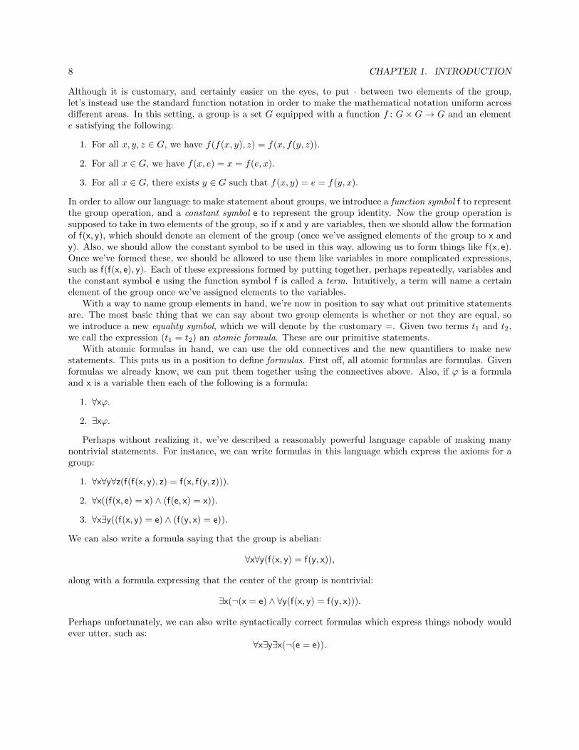
Although it is customary, and certainly easier on the eyes, to put · between two elements of the group,let’s instead use the standard function notation in order to make the mathematical notation uniform acrossdifferent areas. In this setting, a group is a set G equipped with a function f : G×G→ G and an elemente satisfying the following:
1. For all x, y, z ∈ G, we have f(f(x, y), z) = f(x, f(y, z)).
2. For all x ∈ G, we have f(x, e) = x = f(e, x).
3. For all x ∈ G, there exists y ∈ G such that f(x, y) = e = f(y, x).
In order to allow our language to make statement about groups, we introduce a function symbol f to representthe group operation, and a constant symbol e to represent the group identity. Now the group operation issupposed to take in two elements of the group, so if x and y are variables, then we should allow the formationof f(x, y), which should denote an element of the group (once we’ve assigned elements of the group to x andy). Also, we should allow the constant symbol to be used in this way, allowing us to form things like f(x, e).Once we’ve formed these, we should be allowed to use them like variables in more complicated expressions,such as f(f(x, e), y). Each of these expressions formed by putting together, perhaps repeatedly, variables andthe constant symbol e using the function symbol f is called a term. Intuitively, a term will name a certainelement of the group once we’ve assigned elements to the variables.
With a way to name group elements in hand, we’re now in position to say what out primitive statementsare. The most basic thing that we can say about two group elements is whether or not they are equal, sowe introduce a new equality symbol, which we will denote by the customary =. Given two terms t1 and t2,we call the expression (t1 = t2) an atomic formula. These are our primitive statements.
With atomic formulas in hand, we can use the old connectives and the new quantifiers to make newstatements. This puts us in a position to define formulas. First off, all atomic formulas are formulas. Givenformulas we already know, we can put them together using the connectives above. Also, if ϕ is a formulaand x is a variable then each of the following is a formula:
1. ∀xϕ.
2. ∃xϕ.
Perhaps without realizing it, we’ve described a reasonably powerful language capable of making manynontrivial statements. For instance, we can write formulas in this language which express the axioms for agroup:
1. ∀x∀y∀z(f(f(x, y), z) = f(x, f(y, z))).
2. ∀x((f(x, e) = x) ∧ (f(e, x) = x)).
3. ∀x∃y((f(x, y) = e) ∧ (f(y, x) = e)).
We can also write a formula saying that the group is abelian:
∀x∀y(f(x, y) = f(y, x)),
along with a formula expressing that the center of the group is nontrivial:
∃x(¬(x = e) ∧ ∀y(f(x, y) = f(y, x))).
Perhaps unfortunately, we can also write syntactically correct formulas which express things nobody wouldever utter, such as:
∀x∃y∃x(¬(e = e)).

1.2. THE LANGUAGE OF MATHEMATICS 9
What if you want to consider an area other than group theory? Commutative ring theory doesn’t posemuch of a problem, so long as we’re allowed to alter the number of function symbols and constant symbols.We can simply have two function symbols a and m which take two arguments (a to represent addition andm to represent multiplication) and two constant symbols 0 and 1 (0 to represent the additive identity and 1to represent the multiplicative identity). Writing the axioms for commutative rings in this language is fairlystraightforward.
To take something fairly different, what about the theory of partially ordered sets? Recall that a partiallyordered set is a set P equipped with a subset ≤ of P × P , where we write x ≤ y to mean than (x, y) is anelement of this subset, satisfying the following:
1. Reflexive: For all x ∈ P , we have x ≤ x.
2. Antisymmetric: If x, y ∈ P are such that x ≤ y and y ≤ x, then x = y.
3. Transitive: If x, y, z ∈ P are such that x ≤ y and y ≤ z, then x ≤ z.
Analogous to the syntax we used when handling the group operation, we will use notation which puts theordering in front of the two arguments. Doing so may seem odd at this point, given that we are puttingequality in the middle, but we will see that such a convention provides a unifying notation for other similarobjects. We thus introduce a relation symbol R (intuitively representing ≤), and we keep the equality symbol=, but we no longer have a need for constant symbols or function symbols.
In this setting (without constant or function symbols), the only terms that we have (i.e. the only namesfor elements of the partially ordered set) are the variables. However, our atomic formulas are more interestingbecause now there are two basic things we can say about elements of the partial ordering: whether they areequal and whether they are related by the ordering. Thus, our atomic formulas are things of the form t1 = t2and R(t1, t2) where t1 and t2 are terms. From these atomic formulas, we build up all our formulas as above.
We can now write formulas expressing the axioms of partial orderings:
1. ∀xR(x, x).
2. ∀x∀y((R(x, y) ∧ R(y, x))→ (x = y)).
3. ∀x∀y∀z((R(x, y) ∧ R(y, z))→ R(x, z)).
We can also write a formula saying that the partial ordering is a linear ordering:
∀x∀y(R(x, y) ∨ R(y, x)),
along with a formula expressing that there exists a maximal element:
∃x∀y(R(x, y)→ (x = y)).
The general idea is that by leaving flexibility in the types and number of constant symbols, relationsymbols, and function symbols, we’ll be able to handle many areas of mathematics. We call this setupfirst-order logic. An analysis of first-order logic will consume the vast majority of our time.
Now we don’t claim that first-order logic allows us to express everything in mathematics, nor do weclaim that each of the setups above allow us to express everything of importance in that particular field. Forexample, take the group theory setting. We can express that every nonidentity element has order two withthe formula
∀x(f(x, x) = e),
but it seems difficult to say that every element of the group has finite order. The natural guess is
∀x∃n(xn = e),

10 CHAPTER 1. INTRODUCTION
but this poses a problem for two reasons. The first is that our variables are supposed to quantify overelements of the group in question, not the natural numbers. The second is that we put no construction inour language to allow us to write something like xn. For each fixed n, we can express it (for example, forn = 3, we can write f(f(x, x), x) and for n = 4, we can write f(f(f(x, x), x), x)), but it’s not clear how to writeit in a general way without allowing quantification over the natural numbers.
For another example, consider trying to express that a group is simple (i.e. has no nontrivial normalsubgroups). The natural instinct is to quantify over all subsets H of the group G, and say that if it sohappens that H is a normal subgroup, then H is either trivial or everything. However, we have no way toquantify over subsets. It’s certainly possible to allow such constructions, and this gives second-order logic.We can even go further and allow quantifications over sets of subsets (for example, one way of expressingthat a ring is Noetherian is to say that every nonempty set of ideals has a maximal element), which givesthird-order logic, etc.
Newcomers to the field often find it strange that we focus primarily on first-order logic. There aremany reasons to give special attention to first-order logic that we will develop throughout our study, butfor now you should think of it as providing a simple example of a language which is capable of expressingmany important aspects of various branches of mathematics. In fact, we’ll eventually understand that thelimitations of first-order logic are precisely what allow us to prove powerful theorems about it. Moreover,these powerful theorems allow us to deduce interesting mathematical consequences.
1.3 Syntax and Semantics
In the above discussion, we introduced symbols to denote certain concepts (such as using ∧ in place of“and”, ∀ in place of “for all”, and a function symbol f in place of the group operation f). Building andmaintaining a careful distinction between formal symbols and how to interpret them is a fundamental aspectof mathematical logic.
The basic structure of the formal statements that we write down using the symbols, connectives, andquantifiers is known as the syntax of the logic that we’re developing. Syntax corresponds to the grammarof the language in question with no thought given to meaning. Imagine an English instructor who carednothing for the content of your writing, but only cared that it was grammatically correct. That is exactlywhat the syntax of a logic is all about. Syntax is combinatorial in nature and is based on simple rules thatprovide admissible ways to manipulate symbols devoid of any knowledge of their intended meaning.
The manner in which we are permitted (or forced) to interpret the symbols, connectives, and quantifiersis known as the semantics of the the given logic. In a logic, there are often some symbols that we are forcedto interpret in specific rigid way. For instance, in the above examples, we interpret the symbol ∧ to meanand. In the propositional logic setting, this doesn’t settle how to interpret a formula because we haven’tsaid how to interpret the elements of P . We have some flexibility here, but once we assert that we shouldinterpret certain elements of P as true and the others as false, our formulas express statements that areeither true or false.
The first-order logic setting is more complicated. Since we have quantifiers, the first thing that must bedone in order to interpret a formula is to fix a set X which will act as the set of objects over which thequantifiers will range. Once this is done, we can interpret each function symbol f taking k arguments as anactual function f : Xk → X, each relation R symbol taking k arguments as a subset of Xk, and each constantsymbol c as an element of X. Once we’ve fixed what we’re talking about by provided such interpretations,we can view them as expressing something meaningful. For example, if we’ve fixed a group G and interpretedf as the group operation and e as the identity, then the formula
∀x∀y(f(x, y) = f(y, x))
is either true or false, according to whether G is abelian or not.
1.4. THE POINT OF IT ALL 11
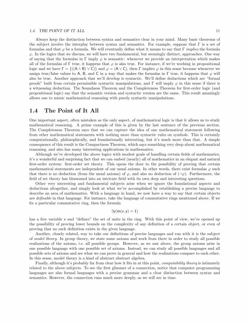
Always keep the distinction between syntax and semantics clear in your mind. Many basic theorems ofthe subject involve the interplay between syntax and semantics. For example, suppose that Γ is a set offormulas and that ϕ be a formula. We will eventually define what it means to say that Γ implies the formulaϕ. In the logics that we discuss, we will have two fundamental, but seemingly distinct, approaches. One wayof saying that the formulas in Γ imply ϕ is semantic: whenever we provide an interpretation which makesall of the formulas of Γ true, it happens that ϕ is also true. For instance, if we’re working in propositionallogic and we have Γ = {((A ∧ B) ∨ C)} and ϕ = (A ∨ C), then Γ implies ϕ in this sense because whenever weassign true/false values to A, B, and C in a way that makes the formulas in Γ true, it happens that ϕ willalso be true. Another approach that we’ll develop is syntactic. We’ll define deductions which are “formalproofs” built from certain permissible syntactic manipulations, and Γ will imply ϕ in this sense if there isa witnessing deduction. The Soundness Theorem and the Completeness Theorem for first-order logic (andpropositional logic) say that the semantic version and syntactic version are the same. This result amazinglyallows one to mimic mathematical reasoning with purely syntactic manipulations.
1.4 The Point of It All
One important aspect, often mistaken as the only aspect, of mathematical logic is that it allows us to studymathematical reasoning. A prime example of this is given by the last sentence of the previous section.The Completeness Theorem says that we can capture the idea of one mathematical statement followingfrom other mathematical statements with nothing more than syntactic rules on symbols. This is certainlycomputationally, philosophically, and foundationally interesting, but it’s much more than that. A simpleconsequence of this result is the Compactness Theorem, which says something very deep about mathematicalreasoning, and also has many interesting applications in mathematics.
Although we’ve developed the above logics with modest goals of handling certain fields of mathematics,it’s a wonderful and surprising fact that we can embed (nearly) all of mathematics in an elegant and naturalfirst-order system: first-order set theory. This opens the door to the possibility of proving that certainmathematical statements are independent of our usual axioms. In other words, there exist formulas ϕ suchthat there is no deduction (from the usual axioms) of ϕ, and also no deduction of (¬ϕ). Furthermore, thefield of set theory has blossomed into an intricate field with its own deep and interesting questions.
Other very interesting and fundamental subjects arise when we ignore the foundational aspects anddeductions altogether, and simply look at what we’ve accomplished by establishing a precise language todescribe an area of mathematics. With a language in hand, we now have a way to say that certain objectsare definable in that language. For instance, take the language of commutative rings mentioned above. If wefix a particular commutative ring, then the formula
∃y(m(x, y) = 1)
has a free variable x and “defines” the set of units in the ring. With this point of view, we’ve opened upthe possibility of proving lower bounds on the complexity of any definition of a certain object, or even ofproving that no such definition exists in the given language.
Another, closely related, way to take our definitions of precise languages and run with it is the subjectof model theory. In group theory, we state some axioms and work from there in order to study all possiblerealizations of the axioms, i.e. all possible groups. However, as we saw above, the group axioms arise inone possible language with one possible set of axioms. Instead, we can study all possible languages and allpossible sets of axioms and see what we can prove in general and how the realizations compare to each other.In this sense, model theory is a kind of abstract abstract algebra.
Finally, although it’s probably far from clear how it fits in at this point, computability theory is intimatelyrelated to the above subjects. To see the first glimmer of a connection, notice that computer programminglanguages are also formal languages with a precise grammar and a clear distinction between syntax andsemantics. However, the connection runs much more deeply, as we will see in time.

12 CHAPTER 1. INTRODUCTION
1.5 Terminology, Notation, and Countable Sets
Definition 1.5.1. We let N = {0, 1, 2, . . . } and we let N+ = N\{0}.
Definition 1.5.2. For each n ∈ N, we let [n] = {m ∈ N : m < n}, so [n] = {0, 1, 2, . . . , n− 1}.
We will often find a need to work with finite sequences, so we establish notation here.
Definition 1.5.3. Let X be a set. Given n ∈ N, we call a function σ : [n] → X a finite sequence from Xof length n. We denote the set of all finite sequences from X of length n by Xn. We use λ to denote theunique sequence of length 0, so X0 = {λ}. Finally, given a finite sequence σ from X, we use the notation|σ| to mean the length of σ.
Definition 1.5.4. Let X be a set. We let X∗ =⋃n∈NX
n, i.e. X∗ is the set of all finite sequences from X.
We denote finite sequences by simply listing the elements in order. For instance, if X = {a, b}, thesequence aababbba is an element of X∗. Sometimes for clarity, we’ll insert commas and instead writea, a, b, a, b, b, b, a.
Definition 1.5.5. If σ, τ ∈ X∗, we denote the concatenation of σ and τ by στ or σ ∗ τ .
Definition 1.5.6. If σ, τ ∈ X∗, we say that σ is an initial segment of τ , a write σ � τ , if σ = τ � [n] forsome n. We say that σ is a proper initial segment of τ , and write σ ≺ τ if σ � τ and σ 6= τ .
Definition 1.5.7. Given a set A, we let P(A) be the set of all subsets of A, and we call P(A) the power setof A.
For example, we have P({1, 2}) = {∅, {1}, {2}, {1, 2}} and P(∅) = {∅}. A simple combinatorial argumentshows that if |A| = n, then |P(A)| = 2n.
Definition 1.5.8. Let A be a set.
• We say that A is countably infinite if there exists a bijection f : N→ A.
• We say that A is countable if it is either finite or countably infinite.
Proposition 1.5.9. Let A be a nonempty set. The following are equivalent:
1. A is countable.
2. There exists a surjection g : N→ A.
3. There exists an injection h : A→ N.
Proposition 1.5.10. We have the following:
1. If A and B are both countable, then A×B is countable.
2. If A0, A1, A2, . . . are all countable, then⋃n∈NAn is countable.
Corollary 1.5.11. If A is countable, then A∗ is countable.
Theorem 1.5.12. The sets Z and Q are countably infinite, but R and P(N) are not countable.

Chapter 2
Induction and Recursion
Proofs by induction and definitions by recursion are fundamental tools when working with the naturalnumbers. However, there are many other places where variants of these ideas apply. In fact, more delicateand exotic proofs by induction and definitions by recursion are two central tools in mathematical logic. We’lleventually see transfinite versions of these ideas that the provide ways to continue into strange new infiniterealms, and these techniques are essential in both set theory and model theory. In this section, we developthe more modest tools of induction and recursion along structures which are generated by one-step processes,like the natural numbers. Occasionally, these types of induction and recursion are called “structural”.
2.1 Induction and Recursion on NWe begin by compiling the basic facts about induction and recursion on the natural numbers. We do notseek to “prove” that inductive arguments or recursive definitions on N are valid methods because they are“obvious” from the normal mathematical perspective which we are adopting. Besides, in order to do so, wewould first have to fix a context in which we are defining N. Eventually, we will indeed carry out such aconstruction in the context of axiomatic set theory, but that is not our current goal. Although the intuitivecontent of the results in this section are probably very familiar, our goal here is simply to carefully codifythese facts in more precise ways to ease the transition to more complicated types of induction and recursion.
Definition 2.1.1. We define S : N→ N by letting S(n) = n+ 1 for all n ∈ N.
We choose the letter S here because it is the first letter of successor. Induction is often stated in thefollowing form: “If 0 has a certain property, and we know that S(n) has the given property whenever nhas the property, then we can conclude that every n ∈ N has the given property”. We state this idea moreformally using sets (and thus avoiding explicit mention of “properties”) because we can always form the setX = {n ∈ N : n has the given property}.
Theorem 2.1.2 (Induction on N - Step Form). Suppose that X ⊆ N is such that 0 ∈ X and S(n) ∈ Xwhenever n ∈ X. We then have X = N.
Definitions by recursion are often described informally as follows: “When defining f(S(n)), we are allowedto refer to the value of f(n) in addition to referring to n”. For instance, let f : N→ N be the factorial functionf(n) = n!. One typically sees f defined by the following recursive definition:
f(0) = 1.
f(S(n)) = S(n) · f(n) for all n ∈ N.
13

14 CHAPTER 2. INDUCTION AND RECURSION
In order to be able to generalize recursion to other situations, we aim to formalize this idea a little moreabstractly and rigorously. In particular, we would prefer to avoid the direct self-reference in the definitionof f .
Suppose then that X is a set and we’re trying to define a function f : N → X recursively. What do weneed? We certainly want to know f(0), and we want to have a “method” telling us how to define f(S(n))from knowledge of n and the value of f(n). If we want to avoid the self-referential appeal to f when invokingthe value of f(n), we need a method telling us what to do next regardless of the actual particular value off(n). That is, we need a method that tells us what to do on any possible value, not just the one the endsup happening to be f(n). Formally, this “method” can be given by a function g : N ×X → X, which tellsus what to do at the next step. Intuitively, this function acts as an iterator. That is, it says if the the lastthing we were working on was input n and it so happened that we set f(n) to equal x ∈ A, then we shoulddefine f(S(n)) to be the value g(n, x).
With all this setup, we now state the theorem which says that no matter what value we want to assignto f(0), and no matter what iterating function g : N × X → X we have, there exists a unique functionf : N→ X obeying the rules.
Theorem 2.1.3 (Recursion on N - Step Form). Let X be a set, let y ∈ X, and let g : N ×X → X. Thereexists a unique function f : N→ X with the following two properties:
1. f(0) = y.
2. f(S(n)) = g(n, f(n)) for all n ∈ N.
In the case of the factorial function, we have X = N, y = 1, and g : N×N→ N defined by g(n, x) = S(n)·x.Theorem 2.1.3 implies that there is a unique function f : N→ N such that:
1. f(0) = y = 1.
2. f(S(n)) = g(n, f(n)) = S(n) · f(n) for all n ∈ N.
Notice how we moved any mention of self-reference out of the definition of g, and pushed all of the weightonto the theorem that asserts the existence and uniqueness of a function that behaves properly, i.e. thatsatisfies both the initial condition and the appropriate recursive equation.
There is another version of induction on N, sometimes called “strong induction”, which appeals to theordering of the natural numbers rather than the stepping of the successor function.
Theorem 2.1.4 (Induction on N - Order Form). Suppose that X ⊆ N is such that n ∈ X whenever m ∈ Xfor all m ∈ N with m < n. We then have X = N.
Notice that there is no need to deal with a separate base case of n = 0, because this is handled vacuouslybecause there is no m ∈ N with m < 0. In other words, if we successfully prove that statement “n ∈ Xwhenever m ∈ X for all m ∈ N with m < n” using no additional assumptions about n, then this statementis true when n = 0, from which we can conclude that 0 ∈ X because the “whenever” clause is trivially truefor n = 0. Of course, there is no harm in proving a separate base case if you are so inclined.
What about recursions that appeal to more than just the previous value? For example, consider theFibonacci sequence f : N→ N defined by f(0) = 0, f(1) = 1, and f(n) = f(n−1)+f(n−2) whenever n ≥ 2.We could certainly alter our previous version of recursion to codify the ability to look back two positions,but it is short-sighted and limiting to force ourselves to only go back a fixed finite number of positions.For example, what if we wanted to define a function f , so that if n ≥ 2 is even, then we use f(n/2) whendefining f(n)? To handle every such possibility, we want to express the ability to use all smaller values.Thus, instead of having a function g : N × X → X, where the second input codes the previous value of f ,we now want to package many values together. The idea is to code all of the previous values into one finitesequence. So when defining f(4), we should have access to the sequence (f(0), f(1), f(2), f(3)). Since we

2.2. GENERATION 15
defined sequences of length n as functions with domain [n], we are really saying that we should have accessto f � [4] when defining f(4). However, to get around this self-reference, we should define our function gthat will take as input an arbitrary finite sequence of elements of X, and tell us what to do next, assumingthat this sequence is the correct code of the first n values of f . Recall that given a set X, we use X∗ todenote the set of all finite sequences of elements of X.
Theorem 2.1.5 (Recursion on N - Order Form). Let X be a set and let g : X∗ → X. There exists a uniquefunction f : N→ X such that
f(n) = g(f � [n])
for all n ∈ N.
Notice that, in contrast to the situation in Theorem 2.1.3, we do not need to include a separate argumentto g that gives the current position n. The reason for this is that we can always obtain n by simply takingthe length of the sequence f � [n].
With this setup, here is how we can handle the Fibonacci numbers. Let X = N, and defined g : N∗ → Nby letting
g(σ) =
0 if |σ| = 0
1 if |σ| = 1
σ(n− 2) + σ(n− 1) if |σ| = n with n ≥ 2.
Theorem 2.1.5 implies that there is a unique function f : N → N with f(n) = g(f � [n]) for all n ∈ N. Wethen have the following:
• f(0) = g(f � [n]) = g(λ) = 0, where we recall that λ is the empty sequence.
• f(1) = g(f � [1]) = g(0) = 1, where the argument 0 to g is the sequence of length 1 whose only elementis 0.
• For all n ≥ 2, we have f(n) = g(f � [n]) = f(n− 2) + f(n− 1).
2.2 Generation
There are many situations throughout mathematics where we want to look at what a certain subset “gener-ates”. For instance, we might have a subset of a group (vector space, ring, etc.), and we want to consider thesubgroup (subspace, ideal, etc.) that the given subset generates. Another example is that we have a subsetof the vertices of a graph, and we want to consider the set of all vertices in the graph that are reachablefrom the ones in the given subset. In Chapter 1, we talked about generating all formulas from primitiveformulas using certain connectives. This situation will arise so frequently in what follows that it’s a goodidea to unify them all in a common framework.
Definition 2.2.1. Let A be a set and let k ∈ N+. A function h : Ak → A is called a k-ary function on A.The number k is called the arity of the function h. A 1-ary function is sometimes called unary and a 2-aryfunction is sometimes called binary.
Definition 2.2.2. Suppose that A is a set, B ⊆ A, and H is a collection of functions such that each h ∈ H isa k-ary function on A for some k ∈ N+. We call (A,B,H) a simple generating system. In such a situation,for each k ∈ N+, we denote the set of k-ary functions in H by Hk.
For example, let A be a group and let B ⊆ A be some subset that contains the identity of A. Supposethat we want to think about the subgroup of A that B generates. The operations in question here are thegroup operation and inversion, so we let H = {h1, h2}, whose elements are defined as follows:

16 CHAPTER 2. INDUCTION AND RECURSION
1. h1 : A2 → A is given by h1(x, y) = x · y for all x, y ∈ A.
2. h2 : A→ A is given by h2(x) = x−1 for all x ∈ A.
Taken together, we then have that (A,B,H) is a simple generating system.For another example, let V be a vector space over R and let B ⊆ V be some subset that contains the
zero vector. Suppose that we want to think about the subspace of V that B generates. The operationsin question consist of vector addition and scalar multiplication, so we let H = {g} ∪ {hr : r ∈ R} whoseelements are defined as follows:
1. g : V 2 → V is given by g(v, w) = v + w for all v, w ∈ V .
2. For each r ∈ R, hr : V → V is given by hr(v) = r · v for all v ∈ V .
Taken together, we then have that (V,B,H) is a simple generating system. Notice that H has uncountablymany functions (one for each r ∈ R) in this example.
There are some situations where the natural functions to put into H are not total, or are “multi-valued”.For instance, in the first example below, we’ll talk about the subfield generated by a certain subset of a field,and we’ll want to include multiplicative inverses for all nonzero elements. When putting a correspondingfunction in H, there is no obvious way to define it on 0.
Definition 2.2.3. Let A be a set and let k ∈ N+. A function h : Ak → P(A) is called a set-valued k-aryfunction on A. We call k the arity of h. A 1-ary set-valued function is sometimes called unary and a 2-aryset-valued function is sometimes called binary.
Definition 2.2.4. Suppose that A is a set, B ⊆ A, and H is a collection of functions such that each h ∈ His a set-valued k-ary function on A for some k ∈ N+. We call (A,B,H) a generating system. In such asituation, for each k ∈ N+, we denote the set of multi-valued k-ary functions in H by Hk.
For example, let K be a field and let B ⊆ K be some subset that contains both 0 and 1. We wantthe subfield of K that B generates. The operations in question here are addition, multiplication, and bothadditive and multiplicative inverses. We thus let H = {h1, h2, h3, h4}, whose elements are defined as follows:
1. h1 : K2 → P(K) is given by h1(a, b) = {a+ b} for all a, b ∈ K.
2. h2 : K2 → P(K) is given by h2(a, b) = {a · b} for all a, b ∈ K.
3. h3 : K → P(K) is given by h3(a) = {−a} for all a ∈ K.
4. h4 : K → P(K) is given by
h4(a) =
{{a−1} if a 6= 0
∅ if a = 0.
Taken together, we have that (K,B,H) is a generating system.For an example where we want to output multiple values, think about generating the vertices reachable
from a given subset of vertices in a directed graph. Since a vertex can have many arrows coming out of it,we may want to throw in several vertices once we reach one. Suppose then that G is a directed graph withvertex set V and edge set E, and let B ⊆ V . We think of the edges as coded by ordered pairs, so E ⊆ V 2.We want to consider the subset of V reachable from B using edges from E. Thus, we want to say that ifwe’ve generated v ∈ V , and w ∈ V is linked to v via some edge, then we should generate w. We thus letH = {h} where h : V → V is defined as follows:
h(v) = {u ∈ V : (v, u) ∈ E}.

2.2. GENERATION 17
Taken together, we have that (V,B,H) is a generating system.Notice that if we have a simple generating system (A,B,H), then we can associate to it the generating
system (A,B,H′) where H′ = {h′ : h ∈ H} where if h : Ak → A is an element of Hk, then h′ : Ak → P(A) isdefined by letting h′(a1, a2, . . . , ak) = {h(a1, a2, . . . , ak)}.
Given a generating system (A,B,H), we want to define the set of elements of A generated from Busing the functions in H. There are many natural ways to do this. We discuss three approaches: the firstapproach is “from above”, and the second and third are “from below”. Each of these descriptions can beslightly simplified for simple generating systems, but it’s not much harder to handle the more general case.Throughout, we will use the following three examples:
1. The first example is the simple generating system where A = N, B = {7}, and H = {h} whereh : R→ R is the function h(x) = 2x.
2. The second example is the simple generating system given by the following group. Let A = S4,B = {id, (1 2), (2 3), (3 4)}, and H = {h1, h2} where h1 is the binary group operation and h2 is theunary inverse function. Here the group operation is function composition, which happens from rightto left. Thus, for example, we have h1((1 2), (2 3)) = (1 2)(2 3) = (1 2 3).
3. The third example is the generating system given by the following directed graph: We have vertex setA = {1, 2, 3, . . . , 8}, edge set
E = {(1, 1), (1, 2), (1, 7), (2, 8), (3, 1), (4, 4), (5, 7), (6, 1), (6, 2), (6, 5), (8, 3)},
In this case, let B = {3} and H = {h} where h : A → A is described above for directed graphs. Forexample, we have h(1) = {1, 2, 7}, h(2) = {8}, and h(7) = ∅.
2.2.1 From Above
Our first approach is a “top-down” one. Given a generating system (A,B,H), we want to apply the elementsof H to tuples from B, perhaps repeatedly, until we form a kind of closure. Instead of thinking about theiteration, think about the final product. As mentioned, we want a set that is closed under the functions inH. This idea leads to the following definition.
Definition 2.2.5. Let (A,B,H) be a generating system, and let J ⊆ A. We say that J is inductive if it hasthe following two properties:
1. B ⊆ J .
2. If k ∈ N+, h ∈ Hk, and a1, a2, . . . , ak ∈ J , then h(a1, a2, . . . , ak) ⊆ J .
Notice that if we working with a simple generating system directly (i.e. not coded as set-valued functions),then we should replace h(a1, a2, . . . , ak) ⊆ J by h(a1, a2, . . . , ak) ∈ J .
Given a generating system (A,B,H), we certainly have a trivial example of an inductive set, since wecan just take A itself. Of course, we don’t want just any old inductive set. Intuitively, we want the smallestone. Let’s take a look at our three examples above in this context.
1. For the first example of a simple generating system given above (where A = R, B = {7}, and H = {h}where h : R→ R is the function h(x) = 2x). In this situation, each of the sets R, Z, N, and {n ∈ N : nis a multiple of 7} is inductive, but none of them seem to be what we want.
2. For the group theory example, we certainly have that S4 is an inductive set, but it’s not obvious ifthere are any others.

18 CHAPTER 2. INDUCTION AND RECURSION
3. In the directed graph example, each of the sets {1, 2, 3, 5, 7, 8}, {1, 2, 3, 4, 7, 8}, and {1, 2, 3, 7, 8} isinductive, and it looks reasonable the last one is the one we are after.
In general, if we want to talk about the smallest inductive subset of A, we need to prove that such anobject exists. Here is where the “from above” idea comes into play. Rather than constructing a smallestinductive set directly (which might be difficult), we instead just intersect them all.
Proposition 2.2.6. Let (A,B,H) be a generating system. There exists a unique inductive set I such thatI ⊆ J for every inductive set J .
Proof. We first prove existence. Let I be the intersection of all inductive sets, i.e.
I = {a ∈ A : a ∈ J for every inductive set J}.
Directly from the definition, we know that if J is inductive, then I ⊆ J . Thus, we need only show that theset I is inductive.
• Let b ∈ B be arbitrary. We have that b ∈ J for every inductive set J (by definition of inductive), sob ∈ I. Therefore, B ⊆ I.
• Suppose that k ∈ N+, h ∈ Hk and a1, a2, . . . , ak ∈ I are arbitrary. Given any inductive set J , wehave a1, a2, . . . , ak ∈ J (since I ⊆ J), hence h(a1, a2, . . . , ak) ⊆ J because J is inductive. Therefore,h(a1, a2, . . . , ak) ⊆ J for every inductive set J , and hence h(a1, a2, . . . , ak) ⊆ I by definition of I.
Putting these together, we conclude that I is inductive.
To see uniqueness, suppose that both I1 and I2 are inductive sets such that I1 ⊆ J and I2 ⊆ J for everyinductive set J . In particular, we then must have both I1 ⊆ I2 and I2 ⊆ I1, so I1 = I2.
Definition 2.2.7. Let (A,B,H) be a generating system. We denote the unique set of the previous propositionby I(A,B,H), or simply by I when the context is clear.
2.2.2 From Below: Building by Levels
The second idea is to make a system of levels, at each new level adding elements of A which are reachablefrom elements already accumulated by applying an element of H. In other words, we start with the elementsof B, then apply functions from H to elements of B to generate (potentially) new elements. From here, wemay need to apply functions from H again to these newly found elements to generate even more elements,etc. Notice that we still want to keep old elements around in this process, because if h ∈ H is binary, wehave b ∈ B, and we generated a new a in the first round, then we will need to include h(b, a) in the nextround. In other words, we should keep a running tab on the elements and repeatedly apply the elementsof H to all combinations generated so far in order to continue climbing up the ladder. Here is the formaldefinition:
Definition 2.2.8. Let (A,B,H) be a generating system. We define a sequence Vn(A,B,H), or simply Vn,of subsets of A recursively as follows:
V0 = B.
Vn+1 = Vn ∪ {c ∈ A : There exists k ∈ N+, h ∈ Hk, and a1, a2, . . . , ak ∈ Vn such that c ∈ h(a1, a2, . . . , ak)}.
Let V (A,B,H) = V =⋃n∈N
Vn = {a ∈ A : There exists n ∈ N with a ∈ Vn}.

2.2. GENERATION 19
Notice that if we work with a simple generating system directly (i.e. not coded as set-valued functions),then we should replace replace the definition of Vn+1 by
Vn+1 = Vn ∪ {h(a1, a2, . . . , ak) : k ∈ N+, h ∈ Hk, and a1, a2, . . . , ak ∈ Vn}.
Let’s take a look at our three examples above in this context.
1. For the first example of a simple generating system given above, we have V0 = B = {7}. Since V0 hasonly element and the unique element h in H is unary with h(7) = 14, we have V1 = {7, 14}. Applyh to each of these elements givens 14 and 28, so V2 = {7, 14, 28}. From here, it is straightforward tocheck that V3 = {7, 14, 28, 56}. In general, it appears that Vn = {7 · 2m : 0 ≤ m ≤ n}, and indeed it ispossible to show this by induction on N. From here, we can conclude that V = {7 · 2m : m ∈ N}. SeeExample 2.3.2.
2. For the group theory example, we start with V0 = B = {id, (1 2), (2 3), (3 4)}. To determine V1, weadd to the V0 the result of inverting all elements of V0, and the result of multiplying pairs of elements ofV0 together. Since every element of V0 is its own inverse, we just need to multiply distinct elements ofV0 together. We have (1 2)(2 3) = (1 2 3), (2 3)(1 2) = (1 3 2), etc. Computing all of the possibilities,we find that
V1 = {id, (1 2), (2 3), (3 4), (1 2 3), (1 3 2), (1 2)(3 4), (2 3 4), (2 4 3)}.
Notice that V1 is closed under inverses, but we now need to multiply elements of V1 together toform new elements of V2. For example, we have (1 2)(1 3 2) = (1 3), so (1 3) ∈ V2. We also have(1 2)(2 3 4) = (1 2 3 4), so (1 2 3 4) ∈ V2. In general, determining V2 explicitly involves performing allof these calculations and collecting the results together. It turns out that V3 has 20 of the 24 elementsin S4 (everything except (1 4), (1 4)(2 3), (1 3 2 4), and (1 4 2 3)), and that V4 = S4. From here, itfollows that Vn = S4 for all n ≥ 4.
3. For the directed graph example, we start with V0 = B = {3}. Now h(3) = {1}, so V1 = {1, 3}. Applyingh to each element of V1, we have h(1) = {1, 2, 7} and h(3) = {1}, so V2 = {1, 2, 3, 7}. Continuing on,we have h(2) = {8} and h(7) = ∅, so V3 = {1, 2, 3, 8}. At the next level, we see that V4 = {1, 2, 3, 8} aswell, and from here it follows that Vn = {1, 2, 3, 8} for all n ≥ 3, and hence V = {1, 2, 3, 8}.
Proposition 2.2.9. , Let (A,B,H) be a generating system. If m ≤ n, then Vm ⊆ Vn.
Proof. Notice that we have Vn ⊆ Vn+1 for all n ∈ N immediately from the definition. From here, thestatement follows by fixing an arbitrary m and inducting on n ≥ m.
Proposition 2.2.10. Let (A,B,H) be a generating system. For all c ∈ V , either c ∈ B or there existsk ∈ N+, h ∈ Hk, and a1, a2, . . . , ak ∈ V with c ∈ h(a1, a2, . . . , ak).
Proof. Let c ∈ V be arbitrary. Since V =⋃n∈N Vn, we know that there exists an n ∈ N with c ∈ Vn. By
well-ordering, there is a smallest m ∈ N with c ∈ Vm. We have two cases.
• Suppose that m = 0. We then have c ∈ V0, so c ∈ B.
• Suppose that m > 0. We then have m − 1 ∈ N, and by choice of m, we know that c /∈ Vm−1. Bydefinition of Vm, this implies that there exists k ∈ N+,h ∈ Hk, and a1, a2, . . . , ak ∈ Vn such thatc ∈ h(a1, a2, . . . , ak).
20 CHAPTER 2. INDUCTION AND RECURSION
2.2.3 From Below: Witnessing Sequences
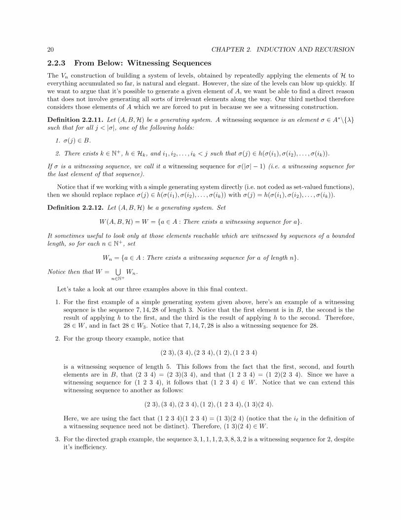
The Vn construction of building a system of levels, obtained by repeatedly applying the elements of H toeverything accumulated so far, is natural and elegant. However, the size of the levels can blow up quickly. Ifwe want to argue that it’s possible to generate a given element of A, we want be able to find a direct reasonthat does not involve generating all sorts of irrelevant elements along the way. Our third method thereforeconsiders those elements of A which we are forced to put in because we see a witnessing construction.
Definition 2.2.11. Let (A,B,H) be a generating system. A witnessing sequence is an element σ ∈ A∗\{λ}such that for all j < |σ|, one of the following holds:
1. σ(j) ∈ B.
2. There exists k ∈ N+, h ∈ Hk, and i1, i2, . . . , ik < j such that σ(j) ∈ h(σ(i1), σ(i2), . . . , σ(ik)).
If σ is a witnessing sequence, we call it a witnessing sequence for σ(|σ| − 1) (i.e. a witnessing sequence forthe last element of that sequence).
Notice that if we working with a simple generating system directly (i.e. not coded as set-valued functions),then we should replace replace σ(j) ∈ h(σ(i1), σ(i2), . . . , σ(ik)) with σ(j) = h(σ(i1), σ(i2), . . . , σ(ik)).
Definition 2.2.12. Let (A,B,H) be a generating system. Set
W (A,B,H) = W = {a ∈ A : There exists a witnessing sequence for a}.
It sometimes useful to look only at those elements reachable which are witnessed by sequences of a boundedlength, so for each n ∈ N+, set
Wn = {a ∈ A : There exists a witnessing sequence for a of length n}.
Notice then that W =⋃
n∈N+
Wn.
Let’s take a look at our three examples above in this final context.
1. For the first example of a simple generating system given above, here’s an example of a witnessingsequence is the sequence 7, 14, 28 of length 3. Notice that the first element is in B, the second is theresult of applying h to the first, and the third is the result of applying h to the second. Therefore,28 ∈W , and in fact 28 ∈W3. Notice that 7, 14, 7, 28 is also a witnessing sequence for 28.
2. For the group theory example, notice that
(2 3), (3 4), (2 3 4), (1 2), (1 2 3 4)
is a witnessing sequence of length 5. This follows from the fact that the first, second, and fourthelements are in B, that (2 3 4) = (2 3)(3 4), and that (1 2 3 4) = (1 2)(2 3 4). Since we have awitnessing sequence for (1 2 3 4), it follows that (1 2 3 4) ∈ W . Notice that we can extend thiswitnessing sequence to another as follows:
(2 3), (3 4), (2 3 4), (1 2), (1 2 3 4), (1 3)(2 4).
Here, we are using the fact that (1 2 3 4)(1 2 3 4) = (1 3)(2 4) (notice that the i` in the definition ofa witnessing sequence need not be distinct). Therefore, (1 3)(2 4) ∈W .
3. For the directed graph example, the sequence 3, 1, 1, 1, 2, 3, 8, 3, 2 is a witnessing sequence for 2, despiteit’s inefficiency.

2.2. GENERATION 21
The first simple observation is that if we truncate a witnessing sequence, what remains is a witnessingsequence.
Proposition 2.2.13. If σ is a witnessing sequence and |σ| = n, then for all m ∈ N+ with m < n we havethat σ � [m] is a witnessing sequence.
Another straightforward observation is that if we concatenate two witnessing sequences, the result is awitnessing sequence.
Proposition 2.2.14. If σ and τ are witnessing sequences, then so is στ .
Finally, since we can always insert “dummy” elements from B (assuming it’s nonempty because otherwisethe result is trivial), we have the following observation.
Proposition 2.2.15. Let (A,B,H) be a generating system. If m ≤ n, then Wm ⊆Wn.
2.2.4 Equivalence of the Definitions
We now prove that the there different constructions that we’ve developed all produce the same set.
Theorem 2.2.16. Given a generating system (A,B,H), we have
I(A,B,H) = V (A,B,H) = W (A,B,H).
Proof. Let I = I(A,B,H), V = V (A,B,H), and W = W (A,B,H).We first show that V is inductive, from which it follows I ⊆ V . Notice first that B = V0 ⊆ V . Suppose
now that k ∈ N+, h ∈ Hk and a1, a2, . . . , ak ∈ V . For each i with 1 ≤ i ≤ k, we can fix an ni withai ∈ Vni . Let m = max{n1, n2, . . . , nk}. Using Proposition 2.2.9, we then have ai ∈ Vm for all i, henceh(a1, a2, . . . , ak) ⊆ Vm+1, and therefore h(a1, a2, . . . , ak) ⊆ V . It follows that V is inductive. By definitionof I, we conclude that I ⊆ V .
We next show that W is inductive, from which it follows that I ⊆ W . Notice first that for every b ∈ B,the sequence b is a witnessing sequence, so b ∈W1 ⊆W . Thus, B ⊆W . Suppose now that k ∈ N+, h ∈ Hk,and a1, a2, . . . , ak ∈ W . Let c ∈ h(a1, a2, . . . , ak) be arbitrary. For each i with 1 ≤ i ≤ k, we can fix awitnessing sequence σi for ai. Using Proposition 2.2.14, we then have that the sequence σ1σ2 · · ·σk obtainedby concatenating all of the σi is a witnessing sequence. Since each of a1, a2, . . . , ak appear as entries in thiswitnessing sequence, if we append the element c onto the end to form σ1σ2 · · ·σkc, we obtain a witnessingsequence for c. Thus, c ∈W . Since c ∈ h(a1, a2, . . . , ak) was arbitrary, it follows that h(a1, a2, . . . , ak) ⊆W .It follows that W is inductive. By definition of I, we conclude that I ⊆W .
We next show that Vn ⊆ I by induction on n ∈ N, from which it follows V ⊆ I. Notice first thatV0 = B ⊆ I because I is inductive. For the inductive step, let n ∈ N be arbitrary with Vn ⊆ I. We showthat Vn+1 ⊆ I. By definition, we have
Vn+1 = Vn ∪ {c ∈ A : There exists k ∈ N+, h ∈ Hk, and a1, a2, . . . , ak ∈ Vn such that c ∈ h(a1, a2, . . . , ak)}.
Now Vn ⊆ I by the inductive hypothesis. Suppose then that k ∈ N+, h ∈ Hk, and a1, a2, . . . , ak ∈ Vn, andfix an arbitrary c ∈ h(a1, a2, . . . , ak). Since Vn ⊆ I, we have a1, a2, . . . , ak ∈ I, hence h(a1, a2, . . . , ak) ⊆ Ibecause I is inductive. Thus, c ∈ I. Since c was arbitrary, we conclude that Vn+1 ⊆ I. By induction, Vn ⊆ Ifor every n ∈ N, hence V ⊆ I.
We finally show that Wn ⊆ I by induction on n ∈ N+, from which it follows W ⊆ I. Since a witnessingsequence of length 1 must just be an element of B, we have W1 = B ⊆ I because I is inductive. For theinductive step, let n ∈ N+ be arbitrary with Wn ⊆ I. We show that Wn+1 ⊆ I. Let σ be an arbitrarywitnessing sequence of length n+1. By Proposition 2.2.13, we then have that that σ � [m+1] is a witnessingsequence of length m + 1 for all m < n. Thus, σ(m) ∈ Wm+1 for all m < n. Since Wm+1 ⊆ Wn whenever

22 CHAPTER 2. INDUCTION AND RECURSION
m < n by Proposition 2.2.15, we conclude that σ(m) ∈ Wn for all m < n, and hence by induction thatσ(m) ∈ I for all m < n. By definition of a witnessing sequence, we know that either σ(n) ∈ B or there existsi1, i2, . . . , ik < n such that σ(n) = h(σ(i1), σ(i2), . . . , σ(ik)). In either case, σ(n) ∈ I because I is inductive.It follows that Wn+1 ⊆ I. By induction, Wn ⊆ I for every n ∈ N+, hence W ⊆ I.
Definition 2.2.17. Let (A,B,H) be a generating system. We denote the common value of I, V,W byG(A,B,H) or simply G.
The ability the view the elements generated in three different ways is often helpful, as we can use themost convenient one when proving a theorem. For example, using Proposition 2.2.10, we obtain the followingcorollary.
Corollary 2.2.18. Let (A,B,H) be a generating system. For all c ∈ G, either c ∈ B or there exists k ∈ N+,h ∈ Hk, and a1, a2, . . . , ak ∈ G with c ∈ h(a1, a2, . . . , ak).
2.3 Step Induction
Now that we have developed the idea of generation, we can formalize the concept of inductive proofs ongenerated sets. In this case, using our top-down definition of I makes the proof trivial.
Proposition 2.3.1 (Step Induction). Let (A,B,H) be a generating system. Suppose that X ⊆ A satisfiesthe following:
1. B ⊆ X.
2. h(a1, a2, . . . , ak) ⊆ X whenever k ∈ N+, h ∈ Hk, and a1, a2, . . . , ak ∈ X.
We then have that G ⊆ X. Thus, if X ⊆ G, we have X = G.
Proof. Our assumption simply asserts that X is inductive, hence G = I ⊆ X immediately from the definitionof I.
Notice that if we are working with a simple generating system directly (i.e. not coded as set-valuedfunctions), then we should replace replace h(a1, a2, . . . , ak) ⊆ X by h(a1, a2, . . . , ak) ∈ X. Proofs thatemploy Proposition 2.3.1 are simply called “proofs by induction” (on G). Proving the first statement thatB ⊆ X is the base case, where we show that all of the initial elements lie in X. Proving the second statementis the inductive step, where we show that if we have some elements of X and apply some h to them, theresult consists entirely of elements of X.
The next example (which was our first example in each of the above constructions) illustrates how wecan sometimes identify G explicitly. Notice that we use two different types of induction in the argument.One direction uses induction on N and the other uses induction on G as just described.
Example 2.3.2. Consider the following simple generating system. Let A = R, B = {7}, and H = {h}where h : R→ R is the function h(x) = 2x. Determine G explicitly.
Proof. As described previously, it appears that we want the set {7, 14, 28, 56, . . . }, which we can write moreformally as {7 · 2n : n ∈ N}. Let X = {7 · 2n : n ∈ N}.
We first show that X ⊆ G by showing that 7 · 2n ∈ G for all n ∈ N by induction (on N). We have7 · 20 = 7 · 1 = 7 ∈ G because B ⊆ G, as G is inductive. Let n ∈ N be arbitrary such that 7 · 2n ∈ G. SinceG is inductive, we know that h(7 · 2n) ∈ G. Now h(7 · 2n) = 2 · 7 · 2n = 7 · 2n+1, so 7 · 2n+1 ∈ G. Therefore,7 · 2n ∈ G for all n ∈ N by induction on N, and hence X ⊆ G.
We now show that G ⊆ X by induction (on G). In other words, we use Proposition 2.3.1 by showingthat X is inductive. Notice that B ⊆ X because 7 = 7 · 1 = 7 · 20 ∈ X. Now let x ∈ X be arbitrary. Fixn ∈ N with x = 7 · 2n. We then have h(x) = 2 · x = 7 · 2n+1 ∈ X. Therefore G ⊆ X by induction.
Combining both containments, we conclude that X = G.

2.4. FREENESS AND STEP RECURSION 23
In many cases, it’s very hard to give a simple explicit description of the set G. This is where inductionin the form of Proposition 2.3.1 really shines, because it allows us to prove something about all elements ofG despite the fact that we might have a hard time getting a handle on what exactly the elements of G looklike. Here’s an example.
Example 2.3.3. Consider the following simple generating system. Let A = Z, B = {6, 183}, and H = {h}where h : A3 → A is given by h(k,m, n) = k ·m+ n. Show that every element of G is divisible by 3.
Proof. Let X = {n ∈ Z : n is divisible by 3}. We prove by induction that G ⊆ X. We first handle the basecase. Notice that 6 = 3 · 2 and 183 = 3 · 61, so B ⊆ X.
We now do the inductive step. Suppose that k,m, n ∈ X, and fix `1, `2, `3 ∈ Z with k = 3`1, m = 3`2,and n = 3`3. We then have
h(k,m, n) = k ·m+ n
= (3`1) · (3`2) + 3`3
= 9`1`2 + 3`3
= 3(3`1`2 + `3),
hence h(k,m, n) ∈ X.By induction (i.e. by Proposition 2.3.1), we hae G ⊆ X. Thus, every element of G is divisible by 3.
2.4 Freeness and Step Recursion
In this section, we restrict attention to simple generating systems for simplicity (and also because all examplesthat we’ll need which support definition by recursion will be simple). Naively, one might expect that astraightforward analogue of Step Form of Recursion on N (Theorem 2.1.3) will carry over to recursion ongenerated sets. The hope would then be that the following is true.
Hope 2.4.1. Suppose that (A,B,H) is a simple generating system and X is a set. Suppose also thatα : B → X and that for every h ∈ Hk, we have a function gh : (A × X)k → X. There exists a uniquefunction f : G→ X with the following two properties:
1. f(b) = α(b) for all b ∈ B.
2. f(h(a1, a2, . . . , ak)) = gh(a1, f(a1), a2, f(a2), . . . , ak, f(ak)) for all h ∈ Hk and all a1, a2, . . . , ak ∈ G.
In other words, suppose that we assign initial values for the elements of B should go (via α), and wehave iterating functions gh for each h ∈ H telling us what to do with each generated element, based onwhat happened to the elements that generated it. Is there necessarily a unique function that satisfies therequirements? Unfortunately, this hope is too good to be true. Intuitively, we may generate an elementa ∈ A in several very different ways, and our different iterating functions conflict on what value we shouldassign to a. Or we loop back and generate an element of A in multiple ways through just one function fromH. Here’s a simple example to see what can go wrong.
Example 2.4.2. Consider the following simple generating system. Let A = {1, 2}, B = {1}, and H = {h}where h : A → A is given by h(1) = 2 and h(2) = 1. Let X = N. Define α : B → N by letting α(1) = 1 anddefine gh : A × N → N by letting gh(a, n) = n + 1. There is no function f : G → N with the following twoproperties:
1. f(b) = α(b) for all b ∈ B.
2. f(h(a)) = gh(a, f(a)) for all a ∈ G.

24 CHAPTER 2. INDUCTION AND RECURSION
The intuition here is that we are starting with 1, which then generates 2 via h, which then loops backaround to generate 1 via h. Now f(1) must agree for each of these possibilities. Here’s the formal argument.
Proof. Notice first that G = {1, 2}. Suppose that f : G→ N satisfies (1) and (2) above. Since f satisfies (1),we must have f(1) = α(1) = 1. By (2), we then have that
f(2) = f(h(1)) = gh(1, f(1)) = f(1) + 1 = 1 + 1 = 2.
By (2) again, it follows that
f(1) = f(h(2)) = gh(2, f(2)) = f(2) + 2 = 1 + 2 = 3,
contradicting the fact that f(1) = 1.
To get around this problem, we want a definition of a “nice” simple generating system. Intuitively, wewant to say something like “every element of G is generated in a unique way”. The following definition is arelatively straightforward way to formulate this idea.
Definition 2.4.3. A simple generating system (A,B,H) is free if the following are true:
1. range(h � Gk) ∩B = ∅ whenever h ∈ Hk.
2. h � Gk is injective for every h ∈ Hk.
3. range(h1 � Gk) ∩ range(h2 � G`) = ∅ whenever h1 ∈ Hk and h2 ∈ H` with h1 6= h2.
Intuitively the first property is saying that we don’t loop around and generate an element of B again(like in the previous bad example), the second is saying that no element of H generates the same elementin two different ways, and the last is saying that there do no exist two different elements of H that generatethe same element.
Here’s a simple example that will be useful in the next section. We’ll see more subtle and importantexamples soon.
Example 2.4.4. Let X be a set. Consider the following simple generating system. Let A = X∗ be the set ofall finite sequences from X, let B = X (viewed as one element sequences), and let H = {hx : x ∈ X} wherehx : X∗ → X∗ is the unary function hx(σ) = xσ. We then have that G = X∗\{λ} and that (A,B,H) is free.
Proof. First notice that X∗\{λ} is inductive because λ /∈ B and hx(σ) 6= λ for all σ ∈ X∗. Next, a simpleinduction on n ∈ N+ shows that Xn ⊆ G for all n ∈ N+, so X∗\{λ} ⊆ G. It follows that G = X∗\{λ}.
We now show that (A,B,H) is free. We have to check the three properties.
• First notice that for any x ∈ X, we have that range(hx � G) ∩ X = ∅ because every element ofrange(hx � G) has length at least 2 (since λ /∈ G).
• For any x ∈ X, we have that hx � G is injective because if hx(σ) = hx(τ), then xσ = xτ , and henceσ = τ .
• Finally, notice that if x, y ∈ X with x 6= y, we have that range(hx � G) ∩ range(hy � G) = ∅ becauseevery elements of range(hx � G) begins with x while every element of range(hy � G) begins with y.
Therefore, (A,B,H) is free.
On to the theorem saying that if a simple generating system is free, then we can perform recursivedefinitions on the elements that are generated.

2.4. FREENESS AND STEP RECURSION 25
Theorem 2.4.5. Suppose that the simple generating system (A,B,H) is free and X is a set. Suppose alsothat α : B → X and that for every h ∈ Hk, we have a function gh : (A ×X)k → X. There exists a uniquefunction f : G→ X with the following two properties:
1. f(b) = α(b) for all b ∈ B.
2. f(h(a1, a2, . . . , ak)) = gh(a1, f(a1), a2, f(a2), . . . , ak, f(ak)) for all h ∈ Hk and all a1, a2, . . . , ak ∈ G.
It turns out that the uniqueness part of the theorem follows by a reasonably straightforward inductionon G, and in fact does not require the assumption that (A,B,H) is free. The hard part is proving existence.We need to define an f , and so we need to take an arbitrary a in A and determine where to send it. Howcan we do that? The basic idea is to build a new simple generating system whose elements are pairs (a, x)where a ∈ A and x ∈ X. Intuitively, we want to generate the pair (a, x) if something (either α or one of thegh functions) tells us that we’d better set f(a) = x if we want to satisfy the above conditions. We then go onto prove (by induction on G) that for every a ∈ A, there exists a unique x ∈ X such that (a, x) is in our newgenerating system. Thus, there are no conflicts, so we can use this to define our function. In other words,we watch the generation of elements of G happen, and carry along added information telling us where weneed to send the elements as we generate them. Now for the details.
Proof. Let A′ = A ×X, B′ = {(b, α(b)) : b ∈ B} ⊆ A′, and H′ = {g′h : h ∈ H} where for each h ∈ Hk, thefunction g′h : (A×X)k → A×X is given by
g′h(a1, x1, a2, x2, . . . , ak, xk) = (h(a1, a2, . . . , ak), gh(a1, x1, a2, x2, . . . , ak, xk)).
Let G′ = G(A′, B′,H′). A straightforward induction (on G′), which we omit, shows that if (a, x) ∈ G′, thena ∈ G. Let
Z = {a ∈ G : There exists a unique x ∈ X such that (a, x) ∈ G′}.We prove by induction (on G) that Z = G.
Base Case: Notice that for each b ∈ B, we have (b, α(b)) ∈ B′ ⊆ G′, hence there exists an x ∈ X suchthat (b, x) ∈ G′. Let b ∈ B be arbitrary, and suppose that y ∈ X is such that (b, y) ∈ G′ and y 6= α(b). Wethen have (b, y) /∈ B′, hence by Corollary 2.2.18 there exists h ∈ Hk and (a1, x1), (a2, x2), . . . , (ak, xk) ∈ G′such that
(b, y) = g′h(a1, x1, a2, x2, . . . , ak, xk)
= (h(a1, a2, . . . , ak), gh(a1, x1, a2, x2, . . . , ak, xk)).
In particular, we then have b = h(a1, a2, . . . , ak). Since a1, a2, . . . , ak ∈ G, this contradicts the fact thatrange(h � Gk) ∩ B = ∅. Therefore, for every b ∈ B, there exists a unique x ∈ X, namely α(b), such that(b, x) ∈ G′. Hence, B ⊆ Z.
Inductive Step: Let h ∈ Hk and a1, a2, . . . , ak ∈ Z be arbitrary. For each i, let xi be the unique elementof X with (ai, xi) ∈ G′. Since G′ is inductive, we have that
g′h(a1, x1, a2, x2, . . . , ak, xk) ∈ G′,
which means that
(h(a1, a2, . . . , ak), gh(a1, x1, a2, x2, . . . , ak, xk)) = g′h(a1, x1, a2, x2, . . . , ak, xk) ∈ G′.
Thus, there exists x ∈ X such that (h(a1, a2, . . . , ak), x) ∈ G′. Suppose now that y ∈ X is such that(h(a1, a2, . . . , ak), y) ∈ G′. We have (h(a1, a2, . . . , ak), y) /∈ B′ because range(h � Gk) ∩ B = ∅, hence by
Corollary 2.2.18 there exists h ∈ H` together with (c1, z1), (c2, z2), . . . , (c`, z`) ∈ G′ such that
(h(a1, a2, . . . , ak), y) = g′h(c1, z1, c2, z2, . . . , ck, zk)
= (h(c1, c2, . . . , c`), gh(c1, z1, c2, z2, . . . , c`, z`)).
26 CHAPTER 2. INDUCTION AND RECURSION
In particular, we have h(a1, a2, . . . , ak) = h(c1, c2, . . . , c`). Since c1, c2, . . . , c` ∈ G, it follows that h = h
because range(h � Gk) ∩ range(h � G`) = ∅ if h 6= h. Since h = h, we also have k = `. Now using the factthat h � Gk is injective, we conclude that ai = ci for all i. Therefore,
y = gh(c1, z1, c2, z2, . . . , c`, z`) = gh(a1, x1, a2, x2, . . . , ak, xk).
Hence, there exists a unique x ∈ X, namely gh(a1, x1, a2, x2, . . . , ak, xk), such that (h(a1, a2, . . . , ak), x) ∈ G′.It now follows by induction that Z = G.
Define f : G → X by letting f(a) be the unique x ∈ X such that (a, x) ∈ G′. We need to check that fsatisfies the required conditions. As stated above, for each b ∈ B, we have (b, α(b)) ∈ G′, so f(b) = α(b).Thus, f satisfies condition (1). Now let h ∈ Hk and a1, a2, . . . , ak ∈ G be arbitrary. We have (ai, f(ai)) ∈ G′for all i, hence
(h(a1, a2, . . . , ak), gh(a1, f(a1), a2, f(a2), . . . , ak, f(ak))) ∈ G′
by the argument in the inductive step above (since G = Z). It follows that
f(h(a1, a2, . . . , ak)) = gh(a1, f(a1), a2, f(a2), . . . , ak, f(ak)),
so f also satisfies condition (2).Finally, we need to show that f is unique. Suppose that f1, f2 : G → X satisfy the conditions (1) and
(2). Let Y = {a ∈ G : f1(a) = f2(a)}. We show that Y = G by induction on G. First notice that for anyb ∈ B we have
f1(b) = α(b) = f2(b),
hence b ∈ Y . It follows that B ⊆ Y . Now let h ∈ Hk and a1, a2, . . . , ak ∈ Y be arbitrary. Since ai ∈ Y foreach i, we have f1(ai) = f2(ai) for each i, and hence
f1(h(a1, a2, . . . , ak)) = gh(a1, f1(a1), a2, f1(a2), . . . , ak, f1(ak))
= gh(a1, f2(a1), a2, f2(a2), . . . , ak, f2(ak))
= f2(h(a1, a2, . . . , ak)).
Thus, h(a1, a2, . . . , ak) ∈ Y . It follows by induction that Y = G, hence f1(a) = f2(a) for all a ∈ G.
2.5 An Illustrative Example
We now embark on a careful formulation and proof of the following statement: If f : A2 → A is associative,i.e. f(a, f(b, c)) = f(f(a, b), c) for all a, b, c ∈ A, then any “grouping” of terms which preserves the orderingof the elements inside the grouping gives the same value. In particular, if we are working in a group A, thenwe can write things like acabba without parentheses, because any allowable insertion of parentheses gives thesame value. Of course, this result is not terribly surprising, and you’ve likely made extensive use of it whendoing algebra. However, a careful proof is a bit tricky, simply because it’s not immediately obvious how todefine “an allowable insertion of parentheses” in a rigorous way.
Throughout this section, let A be a set not containing the symbols [, ], or ?. The symbols [ and ] will codeour parentheses, and ? will code the application of our function. We choose to use square brackets for ourparentheses to distinguish them from the normal parentheses we will use as in our mathematical reasoning.For example, we will plug these symbols into normal mathematical functions, and writing something likeg(() is much more confusing than g([). In other words, we want to distinguish between the parentheses inour expressions and the parentheses we use in the mathematical metatheory to study the expressions. Wewill also use infix notation with ? as usual, rather than the standard function notation, i.e. we will write[a ? b] in place of f(a, b).

2.5. AN ILLUSTRATIVE EXAMPLE 27
Let SymA = A ∪ {[, ], ?}, so SymA is the collection of symbols that we are allowed to work with. Whenthinking about the expressions that we can form using the symbols in SymA, we want to treat everything ina purely syntactic manner. That is, we just want to write down valid sequence of symbols, without thinkingabout how to interpret them. For instance, we want to keep a distinction between the sequence of symbols[a ? b] and the result of evaluating f(a, b) for a given function f : A2 → A.
With all of that in mind, how do we define what a valid expression is? Since we are treating expressions assyntactic objects, every expression will be a sequence of symbols, i.e. will be an element of Sym∗A. However,we don’t want to include every element of Sym∗A, because a[? ? b][ should not considered a reasonableexpression. The way that we obtain all valid expressions is we start with the elements of A, and build upmore complicated expressions by inserting ? between valid expressions, and surrounding with parentheses.
Definition 2.5.1. Define a binary function h : (Sym∗A)2 → Sym∗A by letting h(σ, τ) be the sequence [σ ? τ ].We then have that (Sym∗A, A, {h}) is a simple generating system, where we are viewing the elements of A aslength 1 sequences in SymA. Let ExpA = G(Sym∗A, A, {h}).
For example, suppose that A = {a, b, c}. Typical elements of G(Sym∗A, A, {h}) are c, [b ? [a ? c]] and[c ? [[c ? b] ? a]]. Again, elements of ExpA are just certain special sequences of symbols, so they do not“mean” anything. In order to attach meaning, we need to have a function f : A2 → A that will serve as aninterpretation of ?. Once we have such an f , it seems reasonable that it will provide a way to evaluate theelements of ExpA. That is, with an f : A2 → A in hand, we should be able to define a function from ExpAto A, which essentially replaces each occurrance of the symbol ? by an application of f . The natural wayto define this function is recursively, but in order to do that, we need to know that the generating system isfree.
2.5.1 Proving Freeness
Notice that if we did not use parentheses, i.e. if we defined h′ : (Sym∗A)2 → Sym∗A by letting h′(σ, τ) bethe sequence σ ? τ , then (Sym∗A, A, {h′}) would not be free. For example if A = {a, b, c}, then a ? b ? cwould be an element of G, which can be built up in two distinct ways. More formally, we would haveh′(a ? b, c) = h′(a, b ? c), so h′ � G2 is not be injective.
However, the natural hope is that the inclusion of parentheses forces every element of ExpA to begenerated in a unique way. How can we argue this carefully? Suppose that we have element of ExpA. Couldit be written as both [ϕ1 ? ψ1] and [ϕ2 ? ψ2] in some nontrivial way (i.e. except in the case where ϕ1 = ϕ2
and ψ1 = ψ2)? Since [ϕ1 ? ψ1] and [ϕ2 ? ψ2] are the same sequence of symbols, either ϕ1 = ϕ2, or one of theϕi is a proper initial segment of the other. This is situation that happened in above without parentheses.The sequence a ? b ? c could be decomposed in two ways, and a was a proper initial segment of a ? b.
With this in mind, our first goal will be to prove that no element of ExpA is a proper initial segment ofanother elements of ExpA. To accomplish this task, we will employ a simple “weight” function. The idea isas follows. Given a sequence SymA of symbols, we scan it from left to right. We give the symbol [ a weightof −1, and when we encounter it in a sequence, we think about incurring a small debt that we need to payoff. Analogously, we give the symbol ] a weight of 1, and when we encounter it, we think about paying off asmall debt. Here is the formal definition.
Definition 2.5.2. Define W : Sym∗A → Z as follows. We begin by defining w : SymA → Z in the followingway:
• w(a) = 0 for all a ∈ A.
• w(?) = 0.
• w([) = −1.
• w(]) = 1.

28 CHAPTER 2. INDUCTION AND RECURSION
We then define W : Sym∗A → Z by letting W (λ) = 0 and letting
W (σ) =∑i<|σ|
w(σ(i))
for all σ ∈ Sym∗A\{λ}.
Notice that if σ, τ ∈ Sym∗A, then we trivially have W (στ) = W (σ) +W (τ), since W is just defined as thesums of the weights of the individual symbols. Now the following proposition is intuitively obvious, becauseany valid expression must have an equal number of left and right parentheses, so every debt will be payedoff. Formally, we prove it by induction on the generating system.
Proposition 2.5.3. If ϕ ∈ ExpA, then W (ϕ) = 0.
Proof. The proof is by induction on ϕ. In other words, we let X = {ϕ ∈ ExpA : W (ϕ) = 0}, and we proveby induction that X = ExpA. For the base case, notice that for every a ∈ A, we have that W (a) = 0. Forthe inductive step, let ϕ,ψ ∈ ExpA be arbitrary with W (ϕ) = 0 = W (ψ). We then have that
W ([ϕ ? ψ]) = W ([) +W (ϕ) +W (?) +W (ψ) +W (])
= −1 + 0 + 0 + 0 + 1
= 0.
By induction, it follows that X = ExpA, concluding the proof.
Recall that given σ and τ , we use the notation σ � τ to mean that σ is an initial segment of τ , and useσ ≺ τ to mean that σ is a proper initial segment of τ , i.e. that σ � τ and σ 6= τ .
Proposition 2.5.4. If ϕ ∈ ExpA and σ ≺ ϕ with σ 6= λ, then W (σ) ≤ −1.
Proof. Again, the proof is by induction on ϕ. That is, we let
X = {ϕ ∈ ExpA : For all σ ≺ ϕ with σ 6= λ, we have W (σ) ≤ −1},
and we prove by induction that X = ExpA. Notice that the base case is trivial, because given any a ∈ A,there is no σ 6= λ with σ ≺ a, and hence a ∈ X vacuously.
For the inductive step, let ϕ,ψ ∈ ExpA be arbitrary with ϕ,ψ ∈ X. We prove that [ϕ ? ψ] ∈ X. Letσ ≺ [ϕ ? ψ] be an arbitrary proper initial segment with σ 6= λ. We handle several cases.
• If σ is [, then W (σ) = −1.
• If σ is [τ where τ 6= λ and τ ≺ ϕ, then
W (σ) = −1 +W (τ)
≤ −1− 1 (by induction)
≤ −1.
• If σ is [ϕ or [ϕ?, then
W (σ) = −1 +W (ϕ)
= −1 + 0 (by Proposition 2.5.3)
= −1.

2.5. AN ILLUSTRATIVE EXAMPLE 29
• If σ is [ϕ ? τ , where τ 6= λ and τ ≺ ϕ, then
W (σ) = −1 +W (ϕ) +W (τ)
= −1 + 0 +W (τ) (by Proposition 2.5.3)
≤ −1 + 0− 1 (by induction)
≤ −1.
• Otherwise, σ is [ϕ ? ψ, and
W (σ) = −1 +W (ϕ) +W (ψ)
= −1 + 0 + 0 (by Proposition 2.5.3)
= −1.
Therefore, in all cases, we have W (σ) ≤ −1. Since σ was an arbitrary proper initial segment of [ϕ ? ψ] withσ 6= λ, we conclude that [ϕ ? ψ] ∈ X.
By induction, it follows that X = ExpA, concluding the proof.
Corollary 2.5.5. If ϕ,ψ ∈ ExpA, then ϕ 6≺ ψ.
Proof. This follows by combining Proposition 2.5.3 and Proposition 2.5.4, along with noting that λ /∈ ExpA(which follows by a trivial induction).
We now have the essential tool that will help us prove freeness.
Theorem 2.5.6. The generating system (Sym∗A, A, {h}) is free.
Proof. Notice that our simple generating system only has one binary function, so we need only check twothings.
• First notice that range(h � (ExpA)2) ∩A = ∅ because all elements of range(h) begin with [.
• We now show that range(h � (ExpA)2) is injective. Let ϕ1, ϕ2, ψ1, ψ2 ∈ ExpA be arbitrary withh(ϕ1, ψ1) = h(ϕ2, ψ2). We then have [ϕ1 ? ψ1] = [ϕ2 ? ψ2], hence ϕ1 ? ψ1 = ϕ2 ? ψ2. Since ϕ1 ≺ ϕ2 andϕ2 ≺ ϕ1 are both impossible by Corollary 2.5.5, it follows that ϕ1 = ϕ2. Therefore, ?ψ1 = ?ψ2, and soψ1 = ψ2. It follows that h � (ExpA)2 is injective.
Combining these two facts, we conclude that the generating system is free.
2.5.2 The Result
Since we have established freeness, we can define functions on ExpA recursively. The first such function wedefine is the “evaluation” function.
Definition 2.5.7. Let f : A2 → A. We define a function Evalf : ExpA → A recursively as follows:
• Evalf (a) = a for all a ∈ A.
• Evalf ([ϕ ? ψ]) = f(Evalf (ϕ), Evalf (ψ)) for all ϕ,ψ ∈ ExpA.
Formally, here is how we use freeness to justify the definition. Let α : A → A be the identity map, andlet gh : (Sym∗A×A)2 → A be the function defined by letting gh(σ, a, τ, b) = f(a, b). By Theorem 2.4.5, thereis a unique function Evalf : ExpA → A with the following two properties:

30 CHAPTER 2. INDUCTION AND RECURSION
1. Evalf (a) = α(a) for all a ∈ A.
2. Evalf (h(ϕ,ψ)) = gh(ϕ,Evalf (ϕ), ψ, Evalf (ψ)) for all ϕ,ψ ∈ ExpA.
Unravelling definitions, this is exactly what we wrote above. In the future, we will typically avoid this levelof formality, and just define recursive functions as in the above definition.
Recall that our goal is to prove the following: If f : A2 → A is associative, i.e. f(a, f(b, c)) = f(f(a, b), c)for all a, b, c ∈ A, then any “grouping” of terms which preserves the ordering of the elements inside thegrouping gives the same value. In order to define “preserves the ordering of the elements” carefully, we nowintroduce a function that eliminates all parentheses and occurrences of ? in an element of ExpA. In otherwords, it produces the sequence of elements from A within the given expression, in order of their occurrence.Since the function destroys characters, we’ll call it D. Notice that D is also defined recursively.
Definition 2.5.8. Define a function D : ExpA → A∗ recursively as follows:
• D(a) = a for all a ∈ A.
• D([ϕ?ψ]) = D(ϕ)D(ψ) for all ϕ,ψ ∈ ExpA, where D(ϕ)D(ψ) is just the concatenation of the sequencesD(ϕ) and D(ψ).
With these definitions in hand, we can now precisely state our theorem.
Theorem 2.5.9. Suppose that f : A2 → A is associative, i.e. f(a, f(b, c)) = f(f(a, b), c) for all a, b, c ∈ A.For all ϕ,ψ ∈ ExpA with D(ϕ) = D(ψ), we have Evalf (ϕ) = Evalf (ψ).
In order to prove our theorem, we need to a way to take a sequence σ ∈ A∗ of elements of A, and providea canonical element ϕ ∈ ExpA with D(ϕ) = σ that we can evaluate. The most natural way to do this isto pick a side to group terms on. We’ll choose to “associate to the right”, so that the sequence cabc willproduct [c? [a? [b?c]]]. The definition is intuitively clear, but to make it more precise, we define this groupingrecursively. We could define it recursively on the length of an element of A∗, but its more elegant to use thesimple generating system (A∗, A, {ha : a ∈ A}) where ha : A∗ → A∗ is defined by ha(σ) = aσ. As shown inExample 2.4.4, we know that (A∗, A, {ha : a ∈ A}) is free and we have that G = A∗\{λ}, which justifies thefollowing recursive definition.
Definition 2.5.10. We define R : A∗\{λ} → Sym∗A recursively by letting R(a) = a for all a ∈ A, and lettingR(aσ) = [a ? R(σ)] for all a ∈ A and all σ ∈ A∗\{λ}.
The following result can be proven by a simple induction on the generating system (A∗, A, {ha : a ∈ A}).
Proposition 2.5.11. For all σ ∈ A∗\{λ}, we have R(σ) ∈ ExpA.
Now in order to prove Theorem 2.5.9, we will show that Evalf (ϕ) = Evalf (R(D(ϕ))) for all ϕ ∈ ExpA,i.e. that we can take any ϕ ∈ ExpA, rip it apart so that we see the elements of A in order, and then associateto the right, without affecting the result of the evaluation. We first need the following lemma.
Lemma 2.5.12. Evalf ([R(σ) ? R(τ)]) = Evalf (R(στ)) for all σ, τ ∈ A∗\{λ}.
Proof. Let τ ∈ A∗\{λ} be arbitrary. We prove the result for this fixed τ by induction on A∗\{λ}. That is,we let
X = {σ ∈ A∗\{λ} : Evalf ([R(σ) ? R(τ)]) = Evalf (R(στ))},
and prove by induction on (A∗, A, {ha : a ∈ A}) that X = A∗\{λ}. Suppose first that a ∈ A. We then have
Evalf ([R(a) ? R(τ)]) = Evalf ([a ? R(τ)]) (by definition of R)
= Evalf (R(aτ)) (by definition of R),

2.5. AN ILLUSTRATIVE EXAMPLE 31
so a ∈ X. Suppose now that σ ∈ X and that a ∈ A. We show that aσ ∈ X. We have
Evalf ([R(aσ) ? R(τ)]) = Evalf ([[a ? R(σ)] ? R(τ)]) (by definition of R)
= f(Evalf ([a ? R(σ)]), Evalf (R(τ))) (by definition of Evalf )
= f(f(a,Evalf (R(σ))), Evalf (R(τ))) (by definition of Evalf , using Evalf (a) = a)
= f(a, f(Evalf (R(σ)), Evalf (R(τ)))) (since f is associative)
= f(a,Evalf ([R(σ) ? R(τ)])) (by definition of Evalf )
= f(a,Evalf (R(στ))) (since σ ∈ X)
= Evalf ([a ? R(στ)]) (by definition of Evalf , using Evalf (a) = a)
= Evalf (R(aστ)) (by definition of R),
so aσ ∈ X. The result follows by induction.
We can now prove our key lemma.
Lemma 2.5.13. Evalf (ϕ) = Evalf (R(D(ϕ))) for all ϕ ∈ ExpA.
Proof. By induction on ExpA. If a ∈ A, this is trivial because R(D(a)) = R(a) = a. Suppose thatϕ,ψ ∈ ExpA and the result holds for ϕ and ψ. We then have
Evalf ([ϕ ? ψ]) = f(Evalf (ϕ), Evalf (ψ)) (by definition of Evalf )
= f(Evalf (R(D(ϕ))), Evalf (R(D(ψ)))) (by induction)
= Evalf ([R(D(ϕ)) ? R(D(ψ))]) (by definition of Evalf )
= Evalf (R(D(ϕ)D(ψ))) (by Lemma 2.5.12)
= Evalf (R(D([ϕ ? ψ]))) (by definition of D).
Finally, we can finish the proof of our theorem.
Proof of Theorem 2.5.9. Let ϕ,ψ ∈ ExpA be arbitary such that D(ϕ) = D(ψ). We have
Evalf (ϕ) = Evalf (R(D(ϕ))) (by Lemma 2.5.13)
= Evalf (R(D(ψ))) (since D(ϕ) = D(ψ))
= Evalf (ψ) (by Lemma 2.5.13).
It’s certainly reasonable to ask if the amount of formality and rigor that we used to prove this theoremwas worth it. After all, the result was intuitive and reasonably obvious. These concerns are certainly valid,but working through all of the details in this simple setting will ease the transition to more complicatedarguments.
2.5.3 An Alternate Syntax - Polish Notation
It is standard mathematical practice to place binary operations like ? between two elements (called “infixnotation”) to signify the application of a binary function, and throughout this section we have followed thattradition in building up valid expressions. However, the price that we have pay is that we needed to useparentheses to avoid ambiguity, i.e. to provide freeness. As mentioned, without parentheses, it is not clear

32 CHAPTER 2. INDUCTION AND RECURSION
how to parse a ? b ? c. Should it be [[a ? b] ? c] or [a ? [b ? c]]? If the underlying function f is not associative,then the distinction really matters.
We can of course move the operation to the front and write ?[a, b] instead of [a ? b] similar to how wemight write f(x, y) for a function of two variables. At first sight, this looks even worse because now weintroduced a comma. However, it turns out that we can eliminate all of the extra symbols. That is, wesimply write ?ab without any additional punctuation ,and build further expressions up in this way, thenwe avoid any ambiguity. This syntactic approach is called “Polish notation”. For example, we have thefollowing translations in Polish notation.
• [[a ? b] ? c] =⇒ ? ? abc
• [a ? [b ? c]] =⇒ ?a ? bc.
• [[a ? b] ? [c ? d]] =⇒ ? ? ab ? cd.
We now go about proving that every expression in Polish notation is built up in a unique way. That is, weprove that the corresponding generating system is free. For this section, let A be a set not containing thesymbol ? and let SymA = A ∪ {?}. That is, we no longer include parentheses in SymA.
Definition 2.5.14. Define a binary function h : (Sym∗A)2 → Sym∗A by letting h(σ, τ) be the sequence ?στ .We then have that (Sym∗A, A, {h}) is a simple generating system, where we are viewing the elements of A aslength 1 sequences in Sym∗A. Let PolishExpA = G(Sym∗A, A, {h}).
In order to prove that (Sym∗A, A, {h}) is free, we follow the structure of our previous argument. We startby defining a weight function, but here it is less obvious how to proceed. Unlike the previous case, whereparentheses carried all of the weight and the elements of A were neutral, we now can only have the elementsof A to signify when we have paid off a debt. As a result, instead of giving elements of A a weight of 0, wewill give them weight 1. This leads to the following definition.
Definition 2.5.15. Define W : Sym∗A → Z as follows. We begin by defining w : SymA → Z in the followingway:
• w(a) = 1 for all a ∈ A.
• w(?) = −1.
We then define W : Sym∗A → Z by letting W (λ) = 0 and letting
W (σ) =∑i<|σ|
w(σ(i))
for all σ ∈ Sym∗A\{λ}.
Notice again that if σ, τ ∈ Sym∗A, then we trivially have W (στ) = W (σ) +W (τ). Now when we scan anelement of Sym∗A from left to right, we invoke a debt of −1 when we run across a ?, and end up paying back2 when we encounter elements of A. As a result, valid expressions now have weight 1 instead of weight 0.
Proposition 2.5.16. If ϕ ∈ PolishExpA, then W (ϕ) = 1.
Proof. The proof is by induction on ϕ. Notice that for every a ∈ A, we have that W (a) = 1 by definition.Let ϕ,ψ ∈ PolishExpA be arbitrary with W (ϕ) = 1 = W (ψ). We then have that
W (?ϕψ) = W (?) +W (ϕ) +W (ψ)
= W (ϕ)
= 1.
The result follows by induction.
2.5. AN ILLUSTRATIVE EXAMPLE 33
We now show that proper initial segments of valid expressions have smaller weight. In this case, we donot have to treat λ differently.
Proposition 2.5.17. If ϕ ∈ PolishExpA and σ ≺ ϕ, then W (σ) ≤ 0.
Proof. The proof is by induction on ϕ. Again the base case is trivial, because given any a ∈ A, the onlyσ ≺ a is σ = λ, and we have W (λ) = 0. For the inductive step, assume that ϕ,ψ ∈ PolishExpA and thatthe result holds for ϕ and ψ. We prove the result for ?ϕψ. Let σ ≺ ?ϕψ be arbitrary. We have several cases.
• If σ = λ, then W (σ) = 0.
• If σ is ?τ for some τ ≺ ϕ, then
W (σ) = W (?) +W (τ)
≤ −1 + 0 (by induction)
≤ −1
≤ 0.
• Otherwise, σ is ?ϕτ for some τ ≺ ψ, in which case
W (σ) = W (?) +W (ϕ) +W (τ)
= −1 + 1 +W (τ) (by Proposition 2.5.16)
≤ −1 + 1 + 0 (by induction)
≤ 0.
Thus, the result holds for ?ϕψ.
Corollary 2.5.18. If ϕ,ψ ∈ PolishExpA, then ϕ 6≺ ψ.
Proof. This follows by combining Proposition 2.5.16 and Proposition 2.5.17.
Theorem 2.5.19. The generating system (Sym∗A, A, {h}) is free.
Proof. Notice that our simple generating system only has one binary function, so we need only check twothings.
• First notice that range(h � (PolishExpA)2) ∩A = ∅ because all elements of range(h) begin with ?.
• We now show that range(h � (PolishExpA)2) is injective. Suppose that ϕ1, ϕ2, ψ1, ψ2 ∈ PolishExpAand that h(ϕ1, ψ1) = h(ϕ2, ψ2). We then have ?ϕ1ψ1 = ?ϕ2ψ2, hence ϕ1ψ1 = ϕ2ψ2. Since ϕ1 ≺ ϕ2
and ϕ2 ≺ ϕ1 are both impossible by Corollary 2.5.18, it follows that ϕ1 = ϕ2. Therefore, ψ1 = ψ2. Itfollows that h � (PolishExpA)2 is injective.
Combining these two facts, we conclude that the generating system is free.
If we wanted, we could recursively define an evaluation function (given an f : A2 → A), and proveanalogous results. However, now that we have become acquainted with Polish notation, we can move on toour study of logic.

34 CHAPTER 2. INDUCTION AND RECURSION

Chapter 3
Propositional Logic
3.1 The Syntax of Propositional Logic
We now embark on a careful study of Propositional Logic. As described in Chapter 1, in this setting, we startwith an arbitrary set P , which we think of as our collection of primitive statements. From here, we buildup more complicated statements by repeatedly applying connectives. As in Section 2.5, we have multiplesyntactic approaches that we can follow. We develop both here.
3.1.1 Standard Syntax
We start with the more human readable syntax that uses infix notation for binary connectives, and hencemust employ parentheses in order to avoid ambiguity. In Section 2.5, we used square brackets to distinguishthe formal syntactic constructs from their normal mathematical use. Since we have some experience now,we will forego that pedantic distinction here in order to have more natural looking objects.
Definition 3.1.1. Let P be a nonempty set not containing the symbols (, ),¬,∧,∨, and →, and defineSymP = P ∪ {(, ),¬,∧,∨,→}. Define a unary function h¬ and binary functions h∧, h∨, and h→ on Sym∗Pas follows:
h¬(σ) = (¬σ)
h∧(σ, τ) = (σ ∧ τ)
h∨(σ, τ) = (σ ∨ τ)
h→(σ, τ) = (σ → τ).
We then let FormP = G(Sym∗P , P,H) where H = {h¬, h∧, h∨, h→}.
In other words, we generate more complicated statements by starting with the elements of P and applyingthe functions that introduce connectives. We call the results syntactic objects formulas. We now argue thegenerating system is free by following the outline in Section 2.5.
Definition 3.1.2. Define W : Sym∗P → Z as follows. We begin by defining w : SymP → Z in the followingway:
• w(A) = 0 for all A ∈ P .
• w(3) = 0 for all 3 ∈ {¬,∧,∨,→}.
• w(() = −1.
35

36 CHAPTER 3. PROPOSITIONAL LOGIC
• w()) = 1.
We then define W : Sym∗P → Z by letting W (λ) = 0 and letting
W (σ) =∑i<|σ|
w(σ(i))
for all σ ∈ Sym∗P \{λ}.
With this weight function in hand, the proof that the generating system is free proceeds in the same wayas the example in Section 2.5.
Proposition 3.1.3. We have the following:
1. If ϕ ∈ FormP , then W (ϕ) = 0.
2. If ϕ ∈ FormP and σ ≺ ϕ with σ 6= λ, then W (σ) ≤ −1.
3. If ϕ ∈ FormP , then ϕ 6= λ, and either ϕ is an element of P , or ϕ begins with (.
Proof. These all follow using straightforward inductive arguments (with multiple inductive steps, since wenow have 4 generating functions), the first two of which are completely analogous to Proposition 2.5.3 andProposition 2.5.4.
Corollary 3.1.4. If ϕ,ψ ∈ FormP , then ϕ 6≺ ψ.
Proof. First notice that ϕ 6= λ by part (3) of Proposition 3.1.3. Now apply parts (1) and (2) of Proposition3.1.3.
Theorem 3.1.5. The generating system (Sym∗P , P,H) is free.
Proof. We have to check the three properties.
• First notice that range(h¬ � FormP )∩P = ∅ because all elements of range(h¬) begin with (. Similarly,for any 3 ∈ {∧,∨,→}, we have range(h3 � Form2
P )∩P = ∅ since all elements of range(h3) begin with(.
• We next need to check that each element of H is injective, when restricted to formulas.
Let ϕ,ψ ∈ FormP be arbitrary with h¬(ϕ) = h¬(ψ). We then have (¬ϕ) = (¬ψ), hence ϕ = ψ.Therefore, h¬ � FormP is injective.
Suppose 3 ∈ {∧,∨,→}. Let ϕ1, ϕ2, ψ1, ψ2 ∈ FormP be arbitrary with h3(ϕ1, ψ1) = h3(ϕ2, ψ2).We then have (ϕ13ψ1) = (ϕ23ψ2), hence ϕ13ψ1 = ϕ23ψ2. Since ϕ1 ≺ ϕ2 and ϕ2 ≺ ϕ1 are bothimpossible by Corollary 3.1.4, it follows that ϕ1 = ϕ2. Therefore, 3ψ1 = 3ψ2, and so ψ1 = ψ2. Itfollows that h3 � Form2
P is injective.
• Finally, we must show that two distinct elements of H have disjoint ranges, when restricted to formulas.
Suppose 3 ∈ {∧,∨,→}. Let ϕ,ψ1, ψ2 ∈ FormP be arbitrary with h¬(ϕ) = h3(ψ1, ψ2). We then have(¬ϕ) = (ψ13ψ2), hence ¬ϕ = ψ13ψ2, contradicting the fact that no element of FormP begins with ¬(by part (3) of Proposition 3.1.3). Therefore, range(h¬ � FormP ) ∩ range(h3 � Form2
P ) = ∅.Suppose 31,32 ∈ {∧,∨,→} with 31 6= 32. Let ϕ1, ϕ2, ψ1, ψ2 ∈ FormP be arbitrary with h31(ϕ1, ψ1) =h32
(ϕ2, ψ2). We then have (ϕ131ψ1) = (ϕ232ψ2), hence ϕ131ψ1 = ϕ232ψ2. Since ϕ1 ≺ ϕ2 andϕ2 ≺ ϕ1 are both impossible by Corollary 3.1.4, it follows that ϕ1 = ϕ2. Therefore, 31 = 32, acontradiction. It follows that range(h31
� Form2P ) ∩ range(h32
� Form2P ) = ∅.

3.1. THE SYNTAX OF PROPOSITIONAL LOGIC 37
3.1.2 Polish Notation
Definition 3.1.6. Let P be a set not containing the symbols ¬,∧,∨, and →, and define SymP = P ∪{¬,∧,∨,→}. Define a unary function h¬ and binary functions h∧, h∨, and h→ on Sym∗P as follows:
h¬(σ) = ¬σh∧(σ, τ) = ∧στh∨(σ, τ) = ∨στh→(σ, τ) = → στ.
We then let FormP = G(Sym∗P , P,H) where H = {h¬, h∧, h∨, h→}.
Definition 3.1.7. Define W : Sym∗P → Z as follows. We begin by defining w : SymP → Z in the followingway:
• w(A) = 1 for all A ∈ P .
• w(¬) = 0.
• w(3) = −1 for all 3 ∈ {∧,∨,→}.
We then define W : Sym∗P → Z by letting W (λ) = 0 and letting
W (σ) =∑i<|σ|
w(σ(i))
for all σ ∈ Sym∗P \{λ}.
Proposition 3.1.8. If ϕ ∈ FormP , then W (ϕ) = 1.
Proof. The proof is by induction on ϕ. Notice that for every A ∈ P , we have that W (A) = 1. Suppose thatϕ ∈ FormP is such that W (ϕ) = 1. We then have that
W (¬ϕ) = 0 +W (ϕ)
= W (ϕ)
= 1.
Suppose now that ϕ,ψ ∈ FormP are such that W (ϕ) = 1 = W (ψ), and 3 ∈ {∧,∨,→}. We then have that
W (3ϕψ) = −1 +W (ϕ) +W (ψ)
= −1 + 1 + 1
= 1.
The result follows by induction.
Proposition 3.1.9. If ϕ ∈ FormP and σ ≺ ϕ, then W (σ) ≤ 0.
Proof. The proof is by induction on ϕ. For every A ∈ P , this is trivial because the only σ ≺ A is σ = λ, andwe have W (λ) = 0.
Suppose that ϕ ∈ FormP and the result holds for ϕ. We prove the result for ¬ϕ. Suppose that σ ≺ ¬ϕ.If σ = λ, then W (σ) = 0. Otherwise, σ is ¬τ for some τ ≺ ϕ, in which case
W (σ) = 0 +W (τ)
≤ 0 + 0 (by induction)
≤ 0.

38 CHAPTER 3. PROPOSITIONAL LOGIC
Thus, the result holds for ¬ϕ.
Suppose that ϕ,ψ ∈ FormP and the result holds for ϕ and ψ. Let 3 ∈ {∧,∨,→}. We prove the resultfor 3ϕψ. Suppose that σ ≺ 3ϕψ. If σ = λ, then W (σ) = 0. If σ is 3τ for some τ ≺ ϕ, then
W (σ) = −1 +W (τ)
≤ −1 + 0 (by induction)
≤ −1
≤ 0.
Otherwise, σ is 3ϕτ for some τ ≺ ψ, in which case
W (σ) = −1 +W (ϕ) +W (τ)
= −1 + 1 +W (τ) (by Proposition 3.1.8)
≤ −1 + 1 + 0 (by induction)
≤ 0.
Thus, the result holds for 3ϕψ.
Corollary 3.1.10. If ϕ,ψ ∈ FormP , then ϕ 6≺ ψ.
Proof. This follows by combining Proposition 3.1.8 and Proposition 3.1.9.
Theorem 3.1.11. The generating system (Sym∗P , P,H) is free.
Proof. We have to check the three properties.
• First notice that range(h¬ � FormP )∩P = ∅ because all elements of range(h¬) begin with ¬. Similarly,for any 3 ∈ {∧,∨,→}, we have range(h3 � Form2
P )∩P = ∅ since all elements of range(h3) begin with3.
• We next need to check that each element of H is injective, when restricted to formulas.
Let ϕ,ψ ∈ FormP be arbitrary with h¬(ϕ) = h¬(ψ). We then have ¬ϕ = ¬ψ, hence ϕ = ψ. Therefore,h¬ � FormP is injective.
Suppose 3 ∈ {∧,∨,→}. Let ϕ1, ϕ2, ψ1, ψ2 ∈ FormP be arbitrary with h3(ϕ1, ψ1) = h3(ϕ2, ψ2). Wethen have 3ϕ1ψ1 = 3ϕ2ψ2, hence ϕ1ψ1 = ϕ2ψ2. Since ϕ1 ≺ ϕ2 and ϕ2 ≺ ϕ1 are both impossible byCorollary 3.1.10, it follows that ϕ1 = ϕ2. Therefore, ψ1 = ψ2. Therefore, h3 � Form2
P is injective.
• Finally, we must show that two distinct elements of H have disjoint ranges, when restricted to formulas.
Suppose 3 ∈ {∧,∨,→}. We have range(h¬ � FormP ) ∩ range(h3 � Form2P ) = ∅ because all elements
of range(h¬) begin with ¬ and all elements of range(h3) begin with 3.
Suppose 31,32 ∈ {∧,∨,→} with 31 6= 32. We have range(h31� Form2
P ) ∩ range(h32� Form2
P ) = ∅because all elements of range(h31
) begin with 31 and all elements of range(h32) begin with 32.

3.1. THE SYNTAX OF PROPOSITIONAL LOGIC 39
3.1.3 Official Syntax and Our Abuses of It
Since we should probably fix an official syntax, we’ll choose to use Polish notation. The ability to use fewersymbols is more elegant, and we’ll find that it is more natural to generalize to later context (when we talkabout the possibility of adding new connectives, and when we get to first-order logic). However, as withmany official definitions in mathematics, we’ll ignore and abuse this convention constantly in the interestof readability. For example, we’ll often write things in standard syntax or in more abbreviated forms. Forexample, we’ll write A ∧ B instead of either ∧AB or (A ∧ B). We’ll also write something like
A1 ∧ A2 ∧ · · · ∧ An−1 ∧ An
orn∧
i=1
Ai
in place of (A1 ∧ (A2 ∧ (· · · (An−1 ∧ An) · · · ))) in standard syntax or ∧A1 ∧ A2 · · · ∧ An−1An in Polish notation.Notice that each of these can be defined formally by using a variant of the function R defined in Section 2.5.In general, when we string together multiple applications of an operation (such as ∧) in order, we alwaysassociate to the right.
When it comes to mixing symbols, we’ll follow conventions about “binding” similar to how we think of ·as more binding than + (so that 3 · 5 + 2 is read as (3 · 5) + 2). We think of ¬ as the most binding, so weread ¬A ∧ B as ((¬A) ∧ B). After that, we consider ∧ and ∨ as the next most binding, and → has the leastbinding. We’ll insert parentheses when we wish to override this binding. For example, A ∧ ¬B→ C ∨ D isreally ((A ∧ (¬B))→ (C ∨ D)) while A ∧ (¬B→ C ∨ D) is really (A ∧ ((¬B)→ (C ∨ D))).
3.1.4 Recursive Definitions
Since we’ve shown that our generating system is free, we can define functions recursively. Now it is possibleto define some of functions directly, without appealing to recursion. In such cases, you may wonder why webother. Since our only powerful way to prove things about the set FormP is by induction, and definitionsof functions by recursion are well-suited to induction, it’s simply the easiest way to proceed.
Our first function takes as input a formula ϕ, and outputs the set of element of P that occur within theformula ϕ.
Definition 3.1.12. Given a set P , we define a function OccurProp : FormP → P(P ) recursively as follows:
• OccurProp(A) = {A} for all A ∈ P .
• OccurProp(¬ϕ) = OccurProp(ϕ).
• OccurProp(3ϕψ) = OccurProp(ϕ) ∪OccurProp(ψ) for each 3 ∈ {∧,∨,→}.
In order to make the definition precise, we’re starting with functions α : P → P(P ), gh¬ : Sym∗P×P(P )→P(P ) and gh3
: (Sym∗P × P(P ))2 → P(P ) for each 3 ∈ {∧,∨,→} defined as follows:
• α(A) = {A} for all A ∈ P .
• gh¬(σ, Z) = Z.
• gh3(σ1, Z1, σ2, Z2) = Z1 ∪ Z2 for each 3 ∈ {∧,∨,→}.
We are then appealing to Theorem 2.4.5, which tells us that there is a unique function OccurProp : FormP →P(P ) satisfying the necessary requirements. Of course, this method is more precise, but it’s significantlyless intuitive to use and understand. It’s a good exercise to make sure that you can translate a few more

40 CHAPTER 3. PROPOSITIONAL LOGIC
informal recursive definitions in this way, but once you understand how it works you can safely keep theformalism in the back of your mind (at least until we work to develop formal definitions of computation).
Here’s a basic example of using induction to prove a result based on a recursive definition.
Proposition 3.1.13. We have the following:
1. If Q ⊆ P , then FormQ ⊆ FormP .
2. For any ϕ ∈ FormP , we have ϕ ∈ FormOccurProp(ϕ).
Proof. The first is a straightforward induction on ϕ ∈ FormQ, and is left as an exercise.For the second, the proof is by induction on ϕ ∈ FormP . For the base case, let A ∈ P be arbitrary. Since
OccurProp(A) = {A} and A ∈ Form{A}, we have A ∈ FormOccurProp(A).Let ϕ ∈ FormP be such that the statement is true for ϕ, i.e. such that ϕ ∈ FormOccurProp(ϕ). Since
OccurProp(¬ϕ) = OccurProp(ϕ), it follows that ϕ ∈ FormOccurProp(¬ϕ). Hence, ¬ϕ ∈ FormOccurProp(¬ϕ).Finally, suppose that ϕ,ψ ∈ FormP , that 3 ∈ {∧,∨,→}, and that the statement is true for ϕ and ψ,
i.e. that we have ϕ ∈ FormOccurProp(ϕ) and ψ ∈ FormOccurProp(ψ). Since
OccurProp(ϕ) ⊆ OccurProp(3ϕψ) and OccurProp(ψ) ⊆ OccurProp(3ϕψ)
by definition, it follows from (1) that ϕ,ψ ∈ FormOccurProp(3ϕψ). Therefore, 3ϕψ ∈ FormOccurProp(3ϕψ).
On to some more important recursive definitions.
Definition 3.1.14. We define a function NumConn : FormP → N recursively as follows:
• NumConn(A) = 0 for all A ∈ P .
• NumConn(¬ϕ) = NumConn(ϕ) + 1.
• NumConn(3ϕψ) = NumConn(ϕ) +NumConn(ψ) + 1 for each 3 ∈ {∧,∨,→}.
Although we have defined propositional formulas as certain finite sequences of symbols, it’s more naturalto view them as tree structures. The idea is to view a formula like ∧AB as a tree having one internal node ∧,and then two leaves as children (with A to the left and B to the right). More complicated formulas lead tomore complex trees, but the connectives always serve as internal nodes, and the propositional symbols arethe leaves. In computer science, if we view our propositional formulas as code in a programming language,then these trees are called the syntax trees of the corresponding formulas. From this perspective, NumConngives the number of internal nodes of the corresponding tree. Viewing propositional formulas as trees leadsto another interesting an fundamental recursive function:
Definition 3.1.15. We define a function Depth : FormP → N recursively as follows:
• Depth(A) = 0 for all A ∈ P .
• Depth(¬ϕ) = Depth(ϕ) + 1.
• Depth(3ϕψ) = max{Depth(ϕ), Depth(ψ)}+ 1 for each 3 ∈ {∧,∨,→}.
For example, although NumConn(∨ ∧ AB ∨ CD) = 3, we have Depth(∨ ∧ AB ∨ CD) = 2. Intuitively, thedepth of a formula is the the height of the corresponding syntax tree (or 1 off from the height, depending onhow you count). If we view these syntax trees as electrical circuits built out of logical gates, then the depthis a good measure of how long it takes the electrical circuit to propagate from the inputs (the propositionalsymbols at the leaves) to the output (the root of the tree). In other words, an engineer building a circuit tocompute as quickly as possible would try to minimize the depth of a circuit, rather than just the number ofgates.

3.2. TRUTH ASSIGNMENTS AND SEMANTIC IMPLICATION 41
Definition 3.1.16. We define a function Subform : FormP → P(FormP ) recursively as follows:
• Subform(A) = {A} for all A ∈ P .
• Subform(¬ϕ) = {¬ϕ} ∪ Subform(ϕ).
• Subform(3ϕψ) = {3ϕψ} ∪ Subform(ϕ) ∪ Subform(ψ) for each 3 ∈ {∧,∨,→}.
In other words, Subform takes a formula as input, and produces the set of all formulas that went intobuilding up the formula recursively. For example, we have Subform(∧¬AB) = {∧¬AB,¬A,A,B}. In termsof the syntax trees, Subform(ϕ) is the set of all subtrees of the syntax tree of ϕ, obtained by taking eachnode as a new root. Since our formulas are formally defined as syntactic sequences, a natural question iswhether Subform(ϕ) is the set of subsequences of ϕ that happen to be formulas. This turns out to be true,but is left as an exercise.
We end with a recursive definition of substituting one formula for another.
Definition 3.1.17. Let θ, γ ∈ FormP . We define a function Substθγ : FormP → FormP recursively asfollows.
• Substθγ(A) =
{θ if γ = A
A otherwise.
• Substθγ(¬ϕ) =
{θ if γ = ¬ϕ¬Substθγ(ϕ) otherwise.
• Substθγ(3ϕψ) =
{θ if γ = 3ϕψ
3Substθγ(ϕ)Substθγ(ψ) otherwise.
for each 3 ∈ {∧,∨,→}.
For example, we have
Subst∧AB¬C (∨C→ ∨¬CA¬C) = ∨C→ ∨∧ ABA ∧ AB.
Intuitively, Substθγ(ϕ) finds all subtrees of the syntax tree of ϕ that equal the syntax tree of γ, and replacesall of those with the syntax tree of θ.
3.2 Truth Assignments and Semantic Implication
So far, we’ve treated formulas only as syntactic objects. We briefly alluded to thinking of the syntax treeof a formula as looking like a circuit that computes based on assigning inputs to the propositional symbols,and it is now time to formalize that idea. Recall that, in isolation, a formula like (A ∧ B) ∨ C does not haveany meaning. However, once we assign true/false values to each of A, B, and C, then the formula obtains anatural truth value. We start with the following definition to codify this assigning of values to the symbols.
Definition 3.2.1. Given a set P , a truth assignment on P is a function M : P → {0, 1}.
We are using the number 0 and 1 as natural codings of “false” and “true”. Once we have a truthassignment M on P , we can define the “truth value” of any formula. Of course, the definition is recursive.
Definition 3.2.2. Let P be a set and let M : P → {0, 1} be a truth assignment on P . We define a functionvM : FormP → {0, 1} recursively as follows:

42 CHAPTER 3. PROPOSITIONAL LOGIC
• vM (A) = M(A) for all A ∈ P .
• vM (¬ϕ) =
{1 if vM (ϕ) = 0
0 if vM (ϕ) = 1.
• vM (∧ϕψ) =
0 if vM (ϕ) = 0 and vM (ψ) = 0
0 if vM (ϕ) = 0 and vM (ψ) = 1
0 if vM (ϕ) = 1 and vM (ψ) = 0
1 if vM (ϕ) = 1 and vM (ψ) = 1.
• vM (∨ϕψ) =
0 if vM (ϕ) = 0 and vM (ψ) = 0
1 if vM (ϕ) = 0 and vM (ψ) = 1
1 if vM (ϕ) = 1 and vM (ψ) = 0
1 if vM (ϕ) = 1 and vM (ψ) = 1.
• vM (→ ϕψ) =
1 if vM (ϕ) = 0 and vM (ψ) = 0
1 if vM (ϕ) = 0 and vM (ψ) = 1
0 if vM (ϕ) = 1 and vM (ψ) = 0
1 if vM (ϕ) = 1 and vM (ψ) = 1.
Before moving on, we should note a couple of simple facts about what happens when we either shrink orenlarge the set P . Intuitively, if ϕ ∈ FormQ and Q ⊆ P , then we can extend the truth assignment from Qto P arbitrarily without affecting the value of vM (ϕ). In fact, it seems clear that the value vM (ϕ) dependsonly on the values M(A) for those A that actually occur in ϕ. The next result formalizes these ideas.
Proposition 3.2.3. Let P be a set.
1. Suppose that Q ⊆ P and that M : P → {0, 1} is a truth assignment on P . For all ϕ ∈ FormQ, wehave vM (ϕ) = vM�Q(ϕ).
2. Suppose ϕ ∈ FormP . Whenever M and N are truth assignments on P such that M(A) = N(A) forall A ∈ OccurProp(ϕ), we have vM (ϕ) = vN (ϕ).
Proof. The first part follows by a straightforward induction on ϕ ∈ FormQ, and is left as an exercise. Forthe second, let Q = OccurProp(ϕ). We then have that ϕ ∈ FormQ by Proposition 3.1.13, and so
vM (ϕ) = vM�Q(ϕ) (by part (1))
= vN�Q(ϕ) (since M � Q = N � Q)
= vN (ϕ) (by part (1)).
This completes the proof.
With a method of assigning true/false values to formulas in hand (once we’ve assigned them to P ), weare now in position to use our semantic definitions to given a precise meaning to “The set of formulas Γimplies the formula ϕ”.
Definition 3.2.4. Let P be a set, let Γ ⊆ FormP ,and let ϕ ∈ FormP . We write Γ �P ϕ to mean thatwhenever M is a truth assignment on P with the property that vM (γ) = 1 for all γ ∈ Γ, we have vM (ϕ) = 1.We pronounce Γ �P ϕ as Γ semantically implies ϕ.
3.2. TRUTH ASSIGNMENTS AND SEMANTIC IMPLICATION 43
For example, if P = {A,B,C}, then we claim that {A ∨ B,¬(A ∧ (¬C))} �P B ∨ C. To see this, letM : P → {0, 1} be a truth assignment such that vM (A ∨ B) = 1 and vM (¬(A ∧ (¬C))) = 1. We then havevM (A ∧ (¬C)) = 0, so either vM (A) = 0 or vM (¬C) = 0. We handle the two cases:
• Case 1: Suppose that vM (A) = 0. Since vM (A ∨ B) = 1, it follows that vM (B) = 1, and hencevM (B ∨ C) = 1.
• Case 2: Suppose that vM (¬C) = 0. We then have vM (C) = 1, and hence vM (B ∨ C) = 1.
Therefore, we have vM (B ∨ C) = 1 in either case. It follows that {A ∨ B,¬(A ∧ (¬C))} � B ∨ C.
For another example, we claim that for any set P and any ϕ,ψ ∈ FormP , we have {ϕ → ψ,ϕ} �P ψ.Again, let M : P → {0, 1} be an arbitrary truth assignment such that both vM (ϕ→ ψ) = 1 and vM (ϕ) = 1.If vM (ψ) = 0, it would follows that vM (ϕ→ ψ) = 0, a contradiction. Therefore, vM (ψ) = 1.
As above, it is intuitively clear that in order to understand whether Γ �P ϕ, we need only think aboutthe values of the truth assignments M : P → {0, 1} on the symbols that actually appear in Γ ∪ {ϕ}.
Proposition 3.2.5. Suppose that Q ⊆ P , that Γ ⊆ FormQ, and that ϕ ∈ FormQ. We then have thatΓ �P ϕ if and only if Γ �Q ϕ.
Proof. First notice that Γ ⊆ FormP and ϕ ∈ FormP by Proposition 3.1.13.
Suppose first that Γ �Q ϕ. Let M : P → {0, 1} be a truth assignment such that vM (γ) = 1 for allγ ∈ Γ. By Proposition 3.2.3, we then have that vM�Q(γ) = 1 for all γ ∈ Γ. Since Γ �Q ϕ, it follows thatvM�Q(ϕ) = 1. Using Proposition 3.2.3 again, we conclude that vM (ϕ) = 1. Therefore, Γ �P ϕ.
Suppose conversely that Γ �P ϕ. Let M : Q → {0, 1} be a truth assignment such that vM (γ) = 1 forall γ ∈ Γ. Define a truth assignment N : P → {0, 1} by letting N(A) = M(A) for all A ∈ Q and lettingN(A) = 0 for all A ∈ P\Q. Since N � Q = M , Proposition 3.2.3 implies that vN (γ) = vM (γ) = 1 for allγ ∈ Γ. Since Γ �P ϕ, it follows that vN (ϕ) = 1. Using Proposition 3.2.3 again, we conclude that vM (ϕ) = 1.Therefore, Γ �Q ϕ.
Since the ambient set P does not matter, we will almost always omit the P in �P . We also adopt thefollowing conventions in order to simplify notation.
Notation 3.2.6. Let P be a set.
1. If Γ = ∅, we write � ϕ instead of ∅ � ϕ.
2. If Γ = {γ}, we write γ � ϕ instead of {γ} � ϕ.
Given a finite set Γ ⊆ FormP and a formula ϕ ∈ FormP , there is a basic procedure that we can alwaysfollow in order to determine whether Γ � ϕ. By Proposition 3.2.5, instead of examining all truth assignmentson P , we need only consider truth assignments on the finite set Q of propositional symbols that actuallyoccur in Γ∪{ϕ}. Since Q is a finite set, there are only finitely many such truth assignments. Thus, one way ofdetermining whether Γ � ϕ is simply to check them all. We can systematically arrange the truth assignmentsin a table (see below), where we ensure that we put the the elements of Q in the first columns, and put allelements of Γ ∪ {ϕ} in later columns. We also ensure that if ψ is in a column, then all subformulas of ψappear in an earlier column, which allows us to fill in the table one column at a time. This simple-mindedexhaustive technique is called the method of truth tables.
For example, suppose that we want to show that {(A ∨ B) ∧ C,A→ (¬C)} � (¬C)→ B. We build thefollowing table:
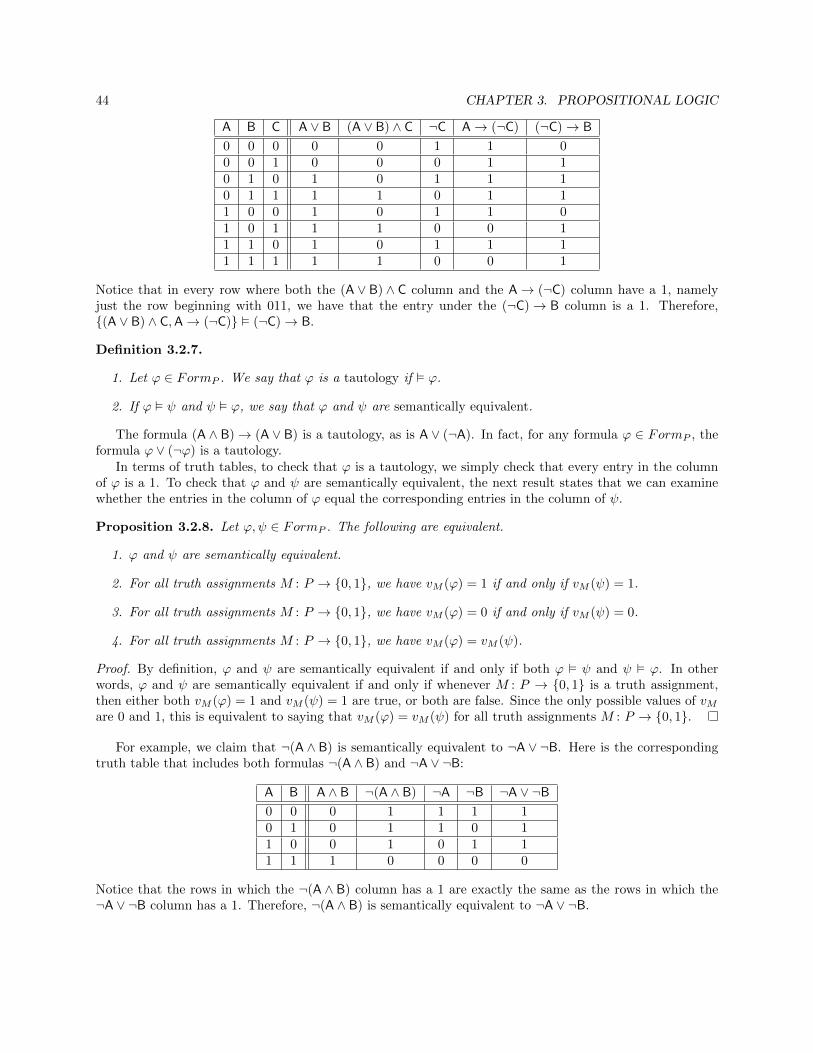
44 CHAPTER 3. PROPOSITIONAL LOGIC
A B C A ∨ B (A ∨ B) ∧ C ¬C A→ (¬C) (¬C)→ B
0 0 0 0 0 1 1 00 0 1 0 0 0 1 10 1 0 1 0 1 1 10 1 1 1 1 0 1 11 0 0 1 0 1 1 01 0 1 1 1 0 0 11 1 0 1 0 1 1 11 1 1 1 1 0 0 1
Notice that in every row where both the (A ∨ B) ∧ C column and the A→ (¬C) column have a 1, namelyjust the row beginning with 011, we have that the entry under the (¬C)→ B column is a 1. Therefore,{(A ∨ B) ∧ C,A→ (¬C)} � (¬C)→ B.
Definition 3.2.7.
1. Let ϕ ∈ FormP . We say that ϕ is a tautology if � ϕ.
2. If ϕ � ψ and ψ � ϕ, we say that ϕ and ψ are semantically equivalent.
The formula (A ∧ B)→ (A ∨ B) is a tautology, as is A ∨ (¬A). In fact, for any formula ϕ ∈ FormP , theformula ϕ ∨ (¬ϕ) is a tautology.
In terms of truth tables, to check that ϕ is a tautology, we simply check that every entry in the columnof ϕ is a 1. To check that ϕ and ψ are semantically equivalent, the next result states that we can examinewhether the entries in the column of ϕ equal the corresponding entries in the column of ψ.
Proposition 3.2.8. Let ϕ,ψ ∈ FormP . The following are equivalent.
1. ϕ and ψ are semantically equivalent.
2. For all truth assignments M : P → {0, 1}, we have vM (ϕ) = 1 if and only if vM (ψ) = 1.
3. For all truth assignments M : P → {0, 1}, we have vM (ϕ) = 0 if and only if vM (ψ) = 0.
4. For all truth assignments M : P → {0, 1}, we have vM (ϕ) = vM (ψ).
Proof. By definition, ϕ and ψ are semantically equivalent if and only if both ϕ � ψ and ψ � ϕ. In otherwords, ϕ and ψ are semantically equivalent if and only if whenever M : P → {0, 1} is a truth assignment,then either both vM (ϕ) = 1 and vM (ψ) = 1 are true, or both are false. Since the only possible values of vMare 0 and 1, this is equivalent to saying that vM (ϕ) = vM (ψ) for all truth assignments M : P → {0, 1}.
For example, we claim that ¬(A ∧ B) is semantically equivalent to ¬A ∨ ¬B. Here is the correspondingtruth table that includes both formulas ¬(A ∧ B) and ¬A ∨ ¬B:
A B A ∧ B ¬(A ∧ B) ¬A ¬B ¬A ∨ ¬B
0 0 0 1 1 1 10 1 0 1 1 0 11 0 0 1 0 1 11 1 1 0 0 0 0
Notice that the rows in which the ¬(A ∧ B) column has a 1 are exactly the same as the rows in which the¬A ∨ ¬B column has a 1. Therefore, ¬(A ∧ B) is semantically equivalent to ¬A ∨ ¬B.

3.2. TRUTH ASSIGNMENTS AND SEMANTIC IMPLICATION 45
For any ϕ ∈ FormP , it’s easy to see that the formulas ϕ and ¬¬ϕ are semantically equivalent. Here isa slightly more interesting example: The formulas ϕ → ψ and ¬ϕ ∨ ψ are semantically equivalent for anyϕ,ψ ∈ FormP . To see this, notice that given an arbitrary truth assignment M : P → {0, 1}, we have
vM (ϕ→ ψ) = 1⇐⇒ vM (ϕ) = 0 or vM (ψ) = 1
⇐⇒ vM (¬ϕ) = 1 or vM (ψ) = 1
⇐⇒ vM (¬ϕ ∨ ψ) = 1.
Thus, vM (ϕ → ψ) = vM (¬ϕ ∨ ψ) for all truth assignments M : P → {0, 1}. Alternatively, we could build atruth table like above, except starting with ϕ and ψ in the first columns rather than specific propositionalsymbols.
Since ϕ → ψ and ¬ϕ ∨ ψ are semantically equivalent for any ϕ,ψ ∈ FormP , it seems redundant toinclude the symbol →. Intuitively, we can replace every occurrence of → using this rule without affectingthe “meaning” of the formula. We now prove a formal version of this statement.
Proposition 3.2.9. Let Form−P be the subset of FormP obtained by omitting h→ from the generatingsystem, i.e. Form−P = G(Sym∗P , P, {h¬, h∧, h∨}). For all ϕ ∈ FormP , there exists ψ ∈ Form−P such that ϕand ψ are semantically equivalent.
Proof. Define a function h : FormP → Form−P recursively as follows:
• h(A) = A for all A ∈ P .
• h(¬ϕ) = ¬h(ϕ) for all ϕ ∈ FormP .
• h(∧ϕψ) = ∧h(ϕ)h(ψ) for all ϕ,ψ ∈ FormP .
• h(∨ϕψ) = ∨h(ϕ)h(ψ) for all ϕ,ψ ∈ FormP .
• h(→ ϕψ) = ∨¬h(ϕ)h(ψ) for all ϕ,ψ ∈ FormP .
We prove that ϕ and h(ϕ) are semantically equivalent for all ϕ ∈ FormP by induction. In other words, welet
X = {ϕ ∈ FormP : ϕ and h(ϕ) are semantically equivalent},and show that X = FormP by proving that X is an inductive set. For the base case, we have h(A) = A forall A ∈ P by definition, so trivially we have that A and h(A) are semantically equivalent for all A ∈ P . Wenow handle the four inductive steps.
• Let ϕ ∈ FormP be arbitrary such that ϕ and h(ϕ) are semantically equivalent. Let M : P → {0, 1} bean arbitrary truth assignment. We have
vM (h(¬ϕ)) = 1⇐⇒ vM (¬h(ϕ)) = 1 (by definition of h)
⇐⇒ vM (h(ϕ)) = 0
⇐⇒ vM (ϕ) = 0 (by Proposition 3.2.8)
⇐⇒ vM (¬ϕ) = 1.
Using Proposition 3.2.8, we conclude that ¬ϕ and h(¬ϕ) are semantically equivalent.
• Let ϕ,ψ ∈ FormP be arbitrary such that ϕ and h(ϕ) are semantically equivalent, and such that ψ andh(ψ) are semantically equivalent. Let M : P → {0, 1} be an arbitrary truth assignment. We have
vM (h(∧ϕφ)) = 1⇐⇒ vM (∧h(ϕ)h(ψ)) = 1 (by definition of h)
⇐⇒ vM (h(ϕ)) = 1 and vM (h(ψ)) = 1
⇐⇒ vM (ϕ) = 1 and vM (ψ) = 1 (by Proposition 3.2.8)
⇐⇒ vM (∧ϕψ) = 1.

46 CHAPTER 3. PROPOSITIONAL LOGIC
Using Proposition 3.2.8, we conclude that ∧ϕφ and h(∧ϕψ) are semantically equivalent.
• Let ϕ,ψ ∈ FormP be arbitrary such that ϕ and h(ϕ) are semantically equivalent, and such that ψ andh(ψ) are semantically equivalent. Let M : P → {0, 1} be an arbitrary truth assignment. We have
vM (h(∨ϕφ)) = 1⇐⇒ vM (∨h(ϕ)h(ψ)) = 1 (by definition of h)
⇐⇒ Either vM (h(ϕ)) = 1 or vM (h(ψ)) = 1
⇐⇒ Either vM (ϕ) = 1 or vM (ψ) = 1 (by Proposition 3.2.8)
⇐⇒ vM (∨ϕψ) = 1.
Using Proposition 3.2.8, we conclude that ∨ϕφ and h(∨ϕψ) are semantically equivalent.
• Let ϕ,ψ ∈ FormP be arbitrary such that ϕ and h(ϕ) are semantically equivalent, and such that ψ andh(ψ) are semantically equivalent. Let M : P → {0, 1} be an arbitrary truth assignment. We have
vM (h(→ ϕφ)) = 1⇐⇒ vM (∨¬h(ϕ)h(ψ)) = 1 (by definition of h)
⇐⇒ Either vM (¬h(ϕ)) = 1 or vM (h(ψ)) = 1
⇐⇒ Either vM (h(ϕ)) = 0 or vM (h(ψ)) = 1
⇐⇒ Either vM (ϕ) = 0 or vM (ψ) = 1 (by Proposition 3.2.8)
⇐⇒ vM (→ ϕψ) = 1.
Using Proposition 3.2.8, we conclude that → ϕφ and h(→ ϕψ) are semantically equivalent.
By induction, it follows that ϕ and h(ϕ) are semantically equivalent for all ϕ ∈ FormP .
In fact, it is possible to improve this result in several orthogonal ways. For instance, since ϕ ∨ ψ and¬((¬ϕ) ∧ (¬ψ)) are semantically equivalent for any ϕ,ψ ∈ FormP , a similar argument to Proposition 3.2.9shows that we can also do away with the function h∨. In other words, every element of FormP is semanticallyequivalent to a formula in G(Sym∗P , P, {h¬, h∧}). We can instead choose to eliminate the ∧ connective. Thatis, since ϕ∧ψ and ¬((¬ϕ)∨ (¬ψ)) are semantically equivalent for any ϕ,ψ ∈ FormP , it follows that elementof FormP is semantically equivalent to a formula in G(Sym∗P , P, {h¬, h∨}).
We can also follows a middle way by keeping both the ∧ and ∨ connectives, but only allow a very limitedversion of negations. In particular, we can restrict negations to only apply to the propositional symbolsdirectly. Here is the formal definition.
Definition 3.2.10. A literal is a element of P ∪ {¬A : A ∈ P}. We denote the set of literals by LitP .
Now we build up our restricted formulas by starting with the literals, and then generating using onlyh∧ and h∨. Following a recursive construction similar to the proof of Proposition 3.2.9, one can show thefollowing.
Proposition 3.2.11. For all ϕ ∈ FormP , there exists ψ ∈ G(Sym∗P , LitP , {h∨, h∧}) such that ϕ and ψ aresemantically equivalent.
Proof. Exercise, although we’ll see a nonrecursive way to prove this fact in the next section.
Finally, we end this section with a semantic way to say that a set of formulas is not contradictory.
Definition 3.2.12. Let P be a set and let Γ ⊆ FormP . We say that Γ is satisfiable if there exists a truthassignment M : P → {0, 1} such that vM (γ) = 1 for all γ ∈ Γ. Otherwise, we say that Γ is unsatisfiable.

3.3. BOOLEAN FUNCTIONS AND CONNECTIVES 47
For example, the set
{A ∨ (B ∧ C),A→ (¬C),B→ C}
is satisfiable, as witnessed by the truth assignment M : P → {0, 1} defined by M(A) = 1, M(B) = 0, andM(C) = 0. In contrast, the set
{A ∧ (B ∨ C),A→ (¬C),B→ C}
is unsatisfiable, which can be verified by a simple exhaustive check. In general, determining if a finiteset of formulas is satisfiable is very difficult. In fact, the computational problem that consists of taking afinite set of formulas, and determining whether it is satisfiable, is one of the most important problems incomputer science. We know of no efficient method that works in general. Any fast algorithm that solvesthe satisfiability problem can be repurposed to solve an enormous number of seemingly disparate problemsthroughout computer science (all problems in the complexity class NP). Unfortunately, we can’t delve intothe theory of NP-completeness here.
3.3 Boolean Functions and Connectives
After seeing that some of our connectives are unnecessary (i.e. can be removed without affecting the expressivepower of our formulas), it is natural to wonder if our choice of connectives is the “right” one. For example,why didn’t we introduce a new connective↔, allow ourselves to build the formula ϕ↔ ψ (or↔ ϕψ in Polishnotation) whenever ϕ,ψ ∈ FormP , and then extend our recursive definition of vM so that
vM (↔ ϕψ) =
1 if vM (ϕ) = 0 and vM (ψ) = 0
0 if vM (ϕ) = 0 and vM (ψ) = 1
0 if vM (ϕ) = 1 and vM (ψ) = 0
1 if vM (ϕ) = 1 and vM (ψ) = 1.
Of course, there is no real need to introduce this connective because for any ϕ,ψ ∈ FormP we would havethat ϕ ↔ ψ is semantically equivalent to (ϕ → ψ) ∧ (ψ → ϕ). Using a recursive construction analogous tothe proof of Proposition 3.2.9, it follows that every formula with this expanded connective is semanticallyequivalent to one without it.
Perhaps we could be more exotic and introduce a new connective � that takes three formulas, allowourselves to build the formula �ϕψθ (here’s an instance when Polish notation becomes important) wheneverϕ,ψ, θ ∈ FormP , and extend our definition of vM so that
vM (�ϕψθ) =
{1 if at least two of vM (ϕ) = 1, vM (ψ) = 1, and vM (θ) = 1
0 otherwise.
In other words, our new connective � is the “majority” connective, i.e. it evaluates the individual truthvalues of the three formulas, and outputs the one that occurs most. It’s not hard (and a good exercise) toshow that for any ϕ,ψ, θ ∈ FormP , there exists α ∈ FormP such that �ϕψθ is semantically equivalent to α.From here, we can again show that every formula with this expanded connective is semantically equivalentto one without it.
We want a general theorem which says that no matter how exotic a connective one invents, it’s alwayspossible to find an element of FormP which is semantically equivalent, and thus our choice of connectives issufficient to express everything we’d ever want. Rather than deal with arbitrary connectives, the real issuehere is whether we can express any possible function taking k true/false values to true/false values.
Definition 3.3.1. Let k ∈ N+. A function f : {0, 1}k → {0, 1} is called a boolean function of arity k.

48 CHAPTER 3. PROPOSITIONAL LOGIC
Definition 3.3.2. Suppose that P = {A0,A1, . . . ,Ak−1}. Given ϕ ∈ FormP , we define a boolean functionBϕ : {0, 1}k → {0, 1} as follows. Given σ ∈ {0, 1}k, define a truth assignment M : P → {0, 1} by lettingM(Ai) = σ(i) for all i, and set Bϕ(σ) = vM (ϕ).
Notice that when P = {A0,A1, . . . ,Ak−1}, then given arbitrary ϕ,ψ ∈ FormP , we have that ϕ and ψ aresemantically equivalent if and only if Bϕ = Bψ, because as we vary σ ∈ {0, 1}k, we are covering all possibletruth assignments. We now show that we can express all possible boolean functions using the connectivesthat we have.
Theorem 3.3.3. Let k ∈ N+ be arbitrary, and let P = {A0,A1, . . . ,Ak−1}. For any boolean functionf : {0, 1}k → {0, 1} of arity k, there exists ϕ ∈ FormP such that f = Bϕ.
In fact, we’ll prove a stronger theorem below which says that we may assume that our formula ϕ is in aparticularly simple form. Before diving into the general argument, let’s look at an example. Suppose thatf : {0, 1}3 → {0, 1} is given by the following table:
0 0 0 10 0 1 00 1 0 10 1 1 01 0 0 01 0 1 01 1 0 11 1 1 1
Suppose we wanted to come up with a formula ϕ such that f = Bϕ. One option is to use a lot of thoughtto come up with an elegant solution. Another is simply to think as follows. Since f(000) = 1, perhaps weshould put
¬A0 ∧ ¬A1 ∧ ¬A2
into the formula somewhere. This subformula will “light up” on the input 000, but not on any other inputs.Similarly, since f(010) = 1, we could imagine putting
¬A0 ∧ A1 ∧ ¬A2
into the formula somewhere to activate on the input 010. If we do the same to the other lines which havevalue 1, we can put all of these pieces together in a manner which makes them all play nice by connectingthem with ∨. Thus, our formula is
(¬A0 ∧ ¬A1 ∧ ¬A2) ∨ (¬A0 ∧ A1 ∧ ¬A2) ∨ (A0 ∧ A1 ∧ ¬A2) ∨ (A0 ∧ A1 ∧ A2).
Since we connecting the various subformulas with the ∨ connective, the entire formula will output 1 exactlywhen at least one of our special subformulas outputs a 1.
Notice the special form of the formula that we have produced in our previous example. We only appliedthe negation symbols to propositional symbols, i.e. the only use of negations was to form literals. From theliterals, we applied the ∧ connective repeatedly to form the subformulas. And then from these formulas weapplied the ∨ connective repeatedly to form our formula. The formulas that can be obtained in this way aresaid to be in disjunctive normal form. Here is the formal definition.
Definition 3.3.4. Let P be a set. We let ConjP = G(Sym∗P , LitP , {h∧}) be the formulas obtained bystarting with the literals and generating using only h∧, and call ConjP the set of conjunctive formulas. Fromhere, we define DNFP = G(Sym∗P , ConjP , {h∨}) to be the formulas obtained by starting with the conjunctiveformulas, and generating using only h∨. The elements of DNFP are said to be in disjunctive normal form.
3.4. SYNTACTIC IMPLICATION 49
We now prove the following theorem, which trivially implies Theorem 3.3.3.
Theorem 3.3.5. Let k ∈ N+ be arbitrary, and let P = {A0,A1, . . . ,Ak−1}. For any boolean functionf : {0, 1}k → {0, 1} of arity k, there exists ϕ ∈ DNFP such that f = Bϕ.
Proof. Let T = {σ ∈ {0, 1}k : f(σ) = 1}. If T = ∅, we may let ϕ be A0 ∧ (¬A0), which is trivially an elementof DNPP . Suppose then that T 6= ∅. For each σ ∈ T , let
ψσ =
k−1∧i=0
θi
where
θi =
{Ai if σ(i) = 1
¬Ai if σ(i) = 0.
For each σ ∈ T , notice that ψσ ∈ ConjP because θi ∈ LitP for all i. Finally, let
ϕ =∨σ∈T
ψσ
and notice that ϕ ∈ DNFP . We then have that f = Bϕ.
3.4 Syntactic Implication
We now work to define a different notion of implication, which is based on syntactic manipulations insteadof a detour through truth assignments and other semantic notions. Our goal is to set up a “proof system”that states the basic implications that we are allowed to write down, and then gives rules about how totransform certain implications into other implications. Although we will fix a choice of basic implicationsand transformation rules, there are many other choices that one can make. Some approaches pride themselveson being minimalistic by using very few basic implications and rules, often at the expense of making thesystem extremely unnatural to work with (but easier to prove things about!). We’ll take a different approachand set down our rules based on the types of steps in a proof that are used naturally throughout mathematics.
Since we will want our rules to be simple and mechanistic, we will ensure that everything in sight isfinite and easily coded by a computer. The objects that we will manipulate will be pairs, where the firstcomponent is a finite sequence of formulas, and the second is a formula. Given a finite sequence S ∈ Form∗Pand a formula ϕ ∈ FormP , we will write S ` ϕ to intuitively mean that there is a formal syntactic proof ofϕ from the assumptions that appear in the sequence S. We begin with the most basic proofs.
Trivial Implications: We can assert S ` ϕ if ϕ appears as an element in the sequence S, i.e. if there existsan i < |S| such that S(i) = γ. We denote these uses of this by writing (AssumeP ), since our conclusionappears in our assumptions.
With these in hand, we describe ways to generate new formal proof from ones that we already have estab-lished. To ease notation, we will write S, γ to mean that we add γ as a new element onto the end of thesequence S. In other words, S, γ means that we concatenate S with the one element sequence γ. In eachcase, we interpret these rules as follows: If we have already established the formal proof(s) appearing abovethe horizontal line, then we are allowed to conclude the formal proof appearing below the horizontal line.
Rules for ∧: We have two rules for ∧-elimination and one for ∧-introduction:
S ` ϕ ∧ ψS ` ϕ
(∧EL)S ` ϕ ∧ ψS ` ψ
(∧ER)S ` ϕ S ` ψS ` ϕ ∧ ψ
(∧I)

50 CHAPTER 3. PROPOSITIONAL LOGIC
Rules for ∨: We have two rules for introducing ∨:
S ` ϕS ` ϕ ∨ ψ
(∨IL)S ` ψ
S ` ϕ ∨ ψ(∨IR)
Rules for →: We have two rules here, one for elimination and for introduction:
S ` ϕ→ ψ
S, ϕ ` ψ(→ E)
S, ϕ ` ψS ` ϕ→ ψ
(→ I)
Rules for proofs by cases: We have two ways to give an argument based on cases:
S, ϕ ` θ S, ψ ` θS, ϕ ∨ ψ ` θ
(∨PC)S, ψ ` ϕ S,¬ψ ` ϕ
S ` ϕ(¬PC)
Rule for proof by contradiction:S,¬ϕ ` ψ S,¬ϕ ` ¬ψ
S ` ϕ(Contr)
Assumption transformation rules:
S ` ϕS, γ ` ϕ
(Expand)S, γ, γ ` ϕS, γ ` ϕ
(Delete)S1, γ1, γ2, S2 ` ϕS1, γ2, γ1, S2 ` ϕ
(Reorder)
As alluded to above, the idea is to start with the trivial formal proofs where the conclusion is included inthe assumptions, and the use the given rules to generate new formal proofs. For a very simple of how theserules can be iterated to form more complex implications, consider the following layering of two rules:
A ∧ B ` A ∧ B (AssumeP ) (1)
A ∧ B ` A (∧EL on 1) (2)
A ∧ B ` A ∨ B (∨I on 2) (3)
Therefore, we conclude that A ∧ B ` A ∨ B. From this example, it’s clear that we are generating newimplications from others, so we can really view this situation as a generating system. Each line of anargument like the one above is a pair, consisting of a sequence from FormP and an element of FormP ,leading us to the following definition.
Definition 3.4.1. Let LineP = Form∗P × FormP .
When viewing the formal proofs as the elements that arise from a generating system, we need to definethe set of elements that we start generating from.
Definition 3.4.2. Let AssumeP = {(S, ϕ) ∈ LineP : There exists i < |S| such that S(i) = ϕ}.
We next need to interpret the various rules as arising from functions in our generating system. In thiscase, it’s most natural to define a generating system that is not simple, although it’s possible to hack togethera simple one that works as well. For an example of one of the functions in our (non-simple) generating system,we define h∧EL : LineP → P(LineP ) as follows:
h∧EL(S, α) =
{{(S, ϕ)} if there exists ϕ,ψ ∈ FormP with α = ϕ ∧ ψ∅ otherwise.
Notice that the above definition makes sense because the system that generated formulas was free, so if thereexists ϕ,ψ ∈ FormP with α = ϕ ∧ ψ, then there is a unique such choice. The definition of h∧EL is similar.

3.4. SYNTACTIC IMPLICATION 51
For the ∧I rule, we define a function h∧I : (LineP )2 → P(LineP ) as follows:
h∧I((S1, ϕ1), (S2, ϕ2)) =
{{(S1, ϕ1 ∧ ϕ2)} if S1 = S2
∅ otherwise.
For the ∨IL rule, we define a function h∨IL : LineP → P(LineP ) as follows:
h∨IL(S, ϕ) = {(S, ϕ ∨ ψ) : ψ ∈ FormP }.
We define h∨IR similarly. It is more complicated, but reasonably straightforward, to write down functionsfor the other rules. Letting H be the collection of all of such functions, we arrive at the following definition.
Definition 3.4.3. Let S ∈ Form∗P and let ϕ ∈ FormP . We write S ` ϕ to mean that
(S, ϕ) ∈ G(LineP , AssumeP ,H).
Let’s go back and examine our argument showing that A ∧ B ` A ∨ B:
A ∧ B ` A ∧ B (AssumeP ) (1)
A ∧ B ` A (∧EL on 1) (2)
A ∧ B ` A ∨ B (∨I on 2) (3)
Notice that this is just a sequence where each line is either in AssumeP , or following from previous lines byapplications of the rules. In other words, we have just written down a witnessing sequence in our generatingsystem.
Definition 3.4.4. A deduction is a witnessing sequence in (LineP , AssumeP ,H).
In other words, a deduction is a kind of “formal proof”, where each step is governed by a limited collectionof simple syntactic manipulations. Here is an an example of deduction showing that ¬A,A ∨ B ` B. Noticethat our deduction here sometimes adds and loses assumptions as it progresses:
¬A,A,¬B ` A (AssumeP ) (1)
¬A,A,¬B ` ¬A (AssumeP ) (2)
¬A,A ` B (Contr on 1 and 2) (3)
¬A,B ` B (AssumeP ) (4)
¬A,A ∨ B ` B (∨PC on 3 and 4) (5)
We are now ready to define a syntactic analogue to our our semantic notion Γ � ϕ.
Definition 3.4.5. Let P be a set, let Γ ⊆ FormP , and let ϕ ∈ FormP . We write Γ ` ϕ if there exists afinite sequence S ∈ Γ∗ such that S ` ϕ. We pronounce Γ ` ϕ as “Γ syntactically implies ϕ”.
Notice the slight distinction between Γ and S in this definition. We are using Γ to denote a set offormulas, and it’s certainly possible that the set Γ is infinite. In contrast, S is a finite sequence of formulasfrom Γ. In particular, S is an ordered collection and allows repetition. More importantly, S must be finite.We enforce this condition because we want our formal proofs to be completely finite, and to follow simplesyntactic rules which can be mechanically checked. We showed above that ¬A,A ∨ B ` B, and hence we canconclude that {¬A,A ∨ B} ` B. If we have a countably infinite set P = {A1,A2,A3, . . . }, we still have that{A1,A2,A3, . . . } ` A1 ∧ A2 because we have A1,A2 ` A1 ∧ A2 (via a simple 3-line deduction).

52 CHAPTER 3. PROPOSITIONAL LOGIC
For a longer example, but reasonably straightforward, example, we give a deduction showing that{A ∨ (B ∧ C) ` (A ∨ B) ∧ (A ∨ C):
A ` A (AssumeP ) (1)
A ` A ∨ B (∨IL on 1) (2)
A ` A ∨ C (∨IL on 1) (3)
A ` (A ∨ B) ∧ (A ∨ C) (∧I on 2 and 3) (4)
B ∧ C ` B ∧ C (AssumeP ) (5)
B ∧ C ` B (∧EL on 5) (6)
B ∧ C ` A ∨ B (∨IR on 6) (7)
B ∧ C ` C (∧ER on 5) (8)
B ∧ C ` A ∨ C (∨IR on 8) (9)
B ∧ C ` (A ∨ B) ∧ (A ∨ C) (∧I on 7 and 9) (10)
A ∨ (B ∧ C) ` (A ∨ B) ∧ (A ∨ C) (∨PC on 4 and 10) (11)
We can also give deductions showing that Γ ` ϕ, even if we don’t have concrete formulas. For example, ourprevious deduction showing that {¬A,A ∨ B} ` B can be generalized to the following result.
Proposition 3.4.6. For any set P and any ϕ,ψ ∈ FormP , we have {¬ϕ,ϕ ∨ ψ} ` ψ.
Proof. Let ϕ,ψ ∈ FormP be arbitrary. We give a deduction.
¬ϕ,ϕ,¬ψ ` ϕ (AssumeP ) (1)
¬ϕ,ϕ,¬ψ ` ¬ϕ (AssumeP ) (2)
¬ϕ,ϕ ` ψ (Contr on 1 and 2) (3)
¬ϕ,ψ ` ψ (AssumeP ) (4)
¬ϕ,ϕ ∨ ψ ` ψ (∨PC on 3 and 4) (5)
Therefore, {¬ϕ,ϕ ∨ ψ} ` ψ.
For a more complicated example, consider the following deduction showing that {(¬ϕ)∨(¬ψ)} ` ¬(ϕ∧ψ)for all ϕ,ψ ∈ FormP :
¬ϕ,¬¬(ϕ ∧ ψ),¬(ϕ ∧ ψ) ` ¬(ϕ ∧ ψ) (AssumeP ) (1)
¬ϕ,¬¬(ϕ ∧ ψ),¬(ϕ ∧ ψ) ` ¬¬(ϕ ∧ ψ) (AssumeP ) (2)
¬ϕ,¬¬(ϕ ∧ ψ) ` ϕ ∧ ψ (Contr on 1 and 2) (3)
¬ϕ,¬¬(ϕ ∧ ψ) ` ϕ (∧EL on 3) (4)
¬ϕ,¬¬(ϕ ∧ ψ) ` ¬ϕ (AssumeP ) (5)
¬ϕ ` ¬(ϕ ∧ ψ) (Contr on 4 and 5) (6)
¬ψ,¬¬(ϕ ∧ ψ),¬(ϕ ∧ ψ) ` ¬(ϕ ∧ ψ) (AssumeP ) (7)
¬ψ,¬¬(ϕ ∧ ψ),¬(ϕ ∧ ψ) ` ¬¬(ϕ ∧ ψ) (AssumeP ) (8)
¬ψ,¬¬(ϕ ∧ ψ) ` ϕ ∧ ψ (Contr on 7 and 8) (9)
¬ψ,¬¬(ϕ ∧ ψ) ` ψ (∧ER on 9) (10)
¬ψ,¬¬(ϕ ∧ ψ) ` ¬ψ (AssumeP ) (11)
¬ψ ` ¬(ϕ ∧ ψ) (Contr on 10 and 11) (12)
(¬ϕ) ∨ (¬ψ) ` ¬(ϕ ∧ ψ) (∨PC on 6 and 12) (13)

3.4. SYNTACTIC IMPLICATION 53
We next show that ` ϕ ∨ ¬ϕ (i.e. that ∅ ` ϕ ∨ ¬ϕ) for all ϕ ∈ FormP , illustrating how we can obtain aconclusion with an empty sequence of assumptions:
ϕ ` ϕ (AssumeP ) (1)
ϕ ` ϕ ∨ ¬ϕ (∨IL on 1) (2)
¬ϕ ` ¬ϕ (AssumeP ) (3)
¬ϕ ` ϕ ∨ ¬ϕ (∨IR on 3) (4)
λ ` ϕ ∨ ¬ϕ (¬PC on 2 and 4) (5)
Just as we defined a semantic way to say that set Γ ⊆ FormP is not contradictory (see our definition ofsatisfiable), we now define a syntactic counterpart.
Definition 3.4.7. Γ is inconsistent if there exists θ ∈ FormP such that Γ ` θ and Γ ` ¬θ. Otherwise, wesay that Γ is consistent.
With all of these definitions and simple examples in hand, we can start to prove some simple results aboutthe relation `.
Proposition 3.4.8. Let Γ1 ⊆ FormP and Γ2 ⊆ FormP be such that Γ1 ⊆ Γ2. If ϕ ∈ FormP is such thatΓ1 ` ϕ, then Γ2 ` ϕ.
Proof. Suppose that Γ1 ` ϕ. We can then fix S ∈ Γ∗1 with S ` ϕ. Since S ∈ Γ∗1 and Γ1 ⊆ Γ2, we have thatS ∈ Γ∗2. Therefore, Γ2 ` ϕ.
Proposition 3.4.9. Suppose that S ∈ Form∗P and ϕ ∈ FormP are such that S ` ϕ. If T is any permutationof S, then T ` ϕ.
Proof. Using the Reorder rule, we can repeatedly flip adjacent elements of S until we form T . More formally,we are using the fact that the set of transpositions
{(1 2), (2 3), (3 4), . . . , (n− 1 n)}
generates the symmetric group on n symbols.
Proposition 3.4.10. If Γ ⊆ FormP is inconsistent, then Γ ` ϕ for all ϕ ∈ FormP .
Proof. Suppose that Γ is inconsistent. Fix θ ∈ FormP with both Γ ` θ and Γ ` ¬θ. By definition, we canthen fix S, T ∈ Γ∗ with both S ` θ and T ` ¬θ. Using the Expand rule together with Proposition 3.4.9, weconclude that ST ` θ and ST ` ¬θ, where ST is the result of concatenating the sequences S and T .
Now let ϕ ∈ FormP be arbitrary. By the Expand rule, we have that ST,¬ϕ ` θ and ST,¬ϕ ` ¬θ (wherethe notation just means that we are concatenating the one element sequence ¬θ onto the end of ST ). Usingthe Contr rule, we conclude that ST ` ϕ. Since ST ∈ Γ∗, it follows that Γ ` ϕ.
Proposition 3.4.11. Let Γ ⊆ FormP and let ϕ ∈ FormP .
1. If Γ ∪ {ϕ} is inconsistent, then Γ ` ¬ϕ.
2. If Γ ∪ {¬ϕ} is inconsistent, then Γ ` ϕ.
Proof.
1. Suppose that Γ ∪ {ϕ} is inconsistent. By Proposition 3.4.10, we then have that Γ ∪ {ϕ} ` ¬ϕ . FixS ∈ (Γ ∪ {ϕ})∗ such that S ` ¬ϕ. By the Expand rule, we then have S, ϕ ` ¬ϕ. Using Proposition3.4.9 and the Delete rule, we can fix T ∈ Γ∗ with T, ϕ ` ¬ϕ. Now we also trivially have T,¬ϕ ` ¬ϕfrom AssumeP . Using the ¬PC rule, it follows that T ` ¬ϕ. Since T ∈ Γ∗, we conclude that Γ ` ¬ϕ.
54 CHAPTER 3. PROPOSITIONAL LOGIC
2. Suppose that Γ ∪ {¬ϕ} is inconsistent. By Proposition 3.4.10, we then have that Γ ∪ {¬ϕ} ` ϕ . FixS ∈ (Γ ∪ {¬ϕ})∗ such that S ` ϕ. By the Expand rule, we then have S,¬ϕ ` ϕ. Using Proposition3.4.9 and the Delete rule, we can fix T ∈ Γ∗ with T,¬ϕ ` ϕ. Now we also trivially have T, ϕ ` ϕ fromAssumeP . Using the ¬PC rule, it follows that T ` ϕ. Since T ∈ Γ∗, we conclude that Γ ` ϕ.
Corollary 3.4.12. Let ϕ ∈ FormP . If Γ ⊆ FormP is consistent, then either Γ ∪ {ϕ} is consistent orΓ ∪ {¬ϕ} is consistent.
Proof. We prove the contrapositive. If both Γ ∪ {ϕ} and Γ ∪ {¬ϕ} are inconsistent, then both Γ ` ¬ϕ andΓ ` ϕ by Proposition 3.4.11, so Γ is inconsistent.
Proposition 3.4.13. Let Γ ⊆ FormP and let ϕ ∈ FormP .
1. If Γ ` ϕ and Γ ∪ {ϕ} ` ψ, then Γ ` ψ.
2. If Γ ` ϕ and Γ ` ϕ→ ψ, then Γ ` ψ.
Proof.
1. Suppose that Γ ` ϕ and Γ ∪ {ϕ} ` ψ. Using Proposition 3.4.8, we conclude that Γ ∪ {¬ϕ} ` ϕ. Nowwe also trivially have Γ ∪ {¬ϕ} ` ¬ϕ, so Γ is inconsistent. Using Proposition 3.4.10, it follows thatΓ ∪ {¬ϕ} ` ψ. By definition, together with the Expand rule, the Delete rule, and Proposition 3.4.9,we can fix S ∈ Γ∗ such that S,¬ϕ ` ψ. Similarly, using the fact that Γ ∪ {ϕ} ` ψ, we can fix T ∈ Γ∗
such that T, ϕ ` ψ. By using the Expand rule and Proposition 3.4.9 again, we have both ST,¬ϕ ` ψand ST, ϕ ` ψ. Applying the ¬PC rule, we conclude that ST ` ϕ. Since ST ∈ Γ∗, it follows thatΓ ` ψ.
2. Suppose that Γ ` ϕ and Γ ` ϕ → ψ. Fix S ∈ Γ with S ` ϕ → ψ. Using the → E rule, we haveS, ϕ ` ψ. Since S ∈ Γ∗, it follows that Γ ∪ {ϕ} ` ψ. Now apply (1).
Since deductions are defined entirely in terms of finite sequences, we also have the following simple result.
Proposition 3.4.14. Γ ` ϕ if and only if there is a finite Γ0 ⊆ Γ such that Γ0 ` ϕ.
Proof. The right-to-left direction is immediate from Proposition 3.4.8. For the left-to-right direction, supposethat Γ ` ϕ. Fix S ∈ Γ∗ such that S ` ϕ. Letting Γ0 be the finite subset of Γ consisting of those elementthat occur in S, we immediately conclude that Γ0 ` ϕ.
Corollary 3.4.15. If every finite subset of Γ is consistent, then Γ is consistent.
Proof. We prove the contrapositive. Suppose that Γ is inconsistent, and fix θ ∈ FormP such that Γ ` θ andΓ ` ¬θ. By Proposition 3.4.14, there exists finite sets Γ0 ⊆ Γ and Γ1 ⊆ Γ such that Γ0 ` θ and Γ1 ` ¬θ.Using Proposition 3.4.8, it follows that Γ0∪Γ1 ` θ and Γ0∪Γ1 ` ¬θ, so Γ0∪Γ1 is a finite inconsistent subsetof Γ.
3.5. SOUNDNESS AND COMPLETENESS 55
3.5 Soundness and Completeness
We now have two notions of implications: the semantic Γ � ϕ and the syntactic Γ ` ϕ. We also have twoways to say that a set of formulas is not contradictory: the semantic notion of satisfiability and the syntacticnotion of consistency. Although these concepts are defined in very different ways, it turns out that thesemantic and syntactic notions are the same in both cases. One direction of each of these equivalences isknown and the Soundness Theorem, and the other direction is known as the Completeness Theorem.
The heart of the Soundness Theorem is the statement that if Γ ` ϕ, then Γ � ϕ. Intuitively, if we have aformal proof of a statement, then whenever we assign true/false values in a way that makes the assumptionstrue, we should expect that the conclusion is also true. More formally, we need need to argue that if wehave a deduction witnessing that Γ ` ϕ, and we have a truth assignment M : P → {0, 1} with the propertythat vM (γ) = 1 for all γ ∈ Γ, then we must have vM (ϕ) = 1. A deduction is just a finite sequence of steps,and a deduction showing that Γ ` ϕ ends with a line T ` ϕ for some T ∈ Γ∗. Now in order to show thatΓ � ϕ, it suffices to show that whenever we have a truth assignment M : P → {0, 1} with the property thatvM (γ) = 1 for all γ that appear in T , then we must have vM (ϕ) = 1. Rather than deal with the last lineof the deduction directly, it is much easier to work through the deduction from beginning to end, and arguethat each line has this property. To do that, what we really want to show is that the elements of AssumePhave this property, and that each of our proof rules preserve this property. In other words, we want to givenan inductive argument on the generating set used to define syntactic implication. In order to carry out thisargument, we extend our notation for � to allow finite sequences of formulas.
Notation 3.5.1. Given S ∈ Form∗P and ϕ ∈ FormP , we write S � ϕ to mean that whenever M is a truthassignment on P with the property that vM (γ) = 1 for all γ that appear in S, we have vM (ϕ) = 1. In otherwords, whenever M is a truth assignment on P with the property that vM (S(i)) = 1 for all i < |S|, we havevM (ϕ) = 1.
Now we are ready to state and prove the Soundness Theorem. As alluded to above, instead of workingwith deductions directly and thinking about going line by line, it is more elegant to organize the argumentas induction on the generating system tied to syntactic implication.
Theorem 3.5.2 (Soundness Theorem). Let P be a set.
1. If Γ ` ϕ, then Γ � ϕ.
2. Every satisfiable set of formulas is consistent.
Proof.
1. We prove the following fact: If S ∈ Form∗P and ϕ ∈ FormP are such that S ` ϕ, then S � ϕ. To seewhy this suffices, suppose that Γ ` ϕ. By definition, we can then fix S ∈ Γ∗ with S ` ϕ. From here wecan conclude that S � ϕ. Since every element of S is an element of Γ, it follows that Γ � ϕ.
We prove the statement “Whenever S ` ϕ, we have S � ϕ” by induction. In other words, if G is theset generated by starting with AssumeP and using our proof rules, and we let
X = {(S, ϕ) ∈ G : S � ϕ},
then we show by induction on G that X = G. We begin by noting that if ϕ appears in the sequence S,then we trivially have S � ϕ by definition. Therefore, (S, ϕ) ∈ X for all (S, ϕ) ∈ AssumeP . We nowhandle the inductive steps, one for each rule.
• We first handle the ∧EL rule. Suppose that S � ϕ ∧ ψ. We need to show that S � ϕ. However,this is straightforward because if M : P → {0, 1} is such that vM (γ) = 1 for all γ appearing in S,then vM (ϕ ∧ ψ) = 1 because S � ϕ ∧ ψ, hence vM (ϕ) = 1. Therefore, S � ϕ. The other ∧ rulesand the ∨ rules are similar.
56 CHAPTER 3. PROPOSITIONAL LOGIC
• Consider→ E rule. Suppose that S � ϕ→ ψ. We need to show that S, ϕ � ψ. Let M : P → {0, 1}be such that vM (γ) = 1 for all γ appearing in S, ϕ. Since S � ϕ → ψ, we have vM (ϕ → ψ) = 1.Since vM (ϕ) = 1, it follows that we must have vM (ψ) = 1. Therefore, S, ϕ � ψ. The → I rule issimilar.
• We now handle the ¬PC rule. Suppose that S, ψ � ϕ and S,¬ψ � ϕ. We need to show that S � ϕ.Let M : P → {0, 1} be such that vM (γ) = 1 for all γ appearing in S. Now either vM (ψ) = 1 orvM (ψ) = 0. If vM (ψ) = 1, then we must have vM (ϕ) = 1 because S, ψ � ϕ. Otherwise, we havevM (ψ) = 0, hence vM (¬ψ) = 1, and thus vM (ϕ) = 1 because S,¬ψ � ϕ. Therefore, S � ϕ. The∨PC rule is similar.
• Consider the Contr rule. Suppose that S,¬ϕ � ψ and S,¬ϕ � ¬ψ. We need to show that S � ϕ.Let M : P → {0, 1} be such that vM (γ) = 1 for all γ appearing in S. Suppose instead thatvM (ϕ) = 0. We then have vM (¬ϕ) = 1, and using the fact that S,¬ϕ � ψ and S,¬ϕ � ¬ψ, weconclude that both vM (ψ) = 1 and vM (¬ψ) = 1 . This is a contradiction, hence we must havevM (ϕ) = 1. Therefore, S � ϕ.
• The assumption transformation rules are all completely straightforward.
By induction, it follows that X = G, which is to say that whenever S ` ϕ, we have S � ϕ. By thecomments above, statement (1) follows
2. Let Γ be a satisfiable set of formulas. Fix a truth assignment M : P → {0, 1} such that vM (γ) = 1 forall γ ∈ Γ. Suppose instead that Γ is inconsistent, and fix θ ∈ FormP such that Γ ` θ and Γ ` ¬θ. Wethen have Γ � θ and Γ � ¬θ by part (1), hence both vM (θ) = 1 and vM (¬θ) = 1, a contradiction. Itfollows that Γ must be consistent.
The Completeness Theorem is the converse (of both parts) of the Soundness Theorem. In order words, itsays that (1) If Γ � ϕ, then Γ ` ϕ and (2) every consistent set of formulas is satisfiable. Part (1) looks quitedifficult to tackle directly (think about the amount of cleverness that went into finding the simple deductionsabove), so instead we go after (2) first and then use it to prove (1).
Assume then that we have a consistent set of formulas Γ ⊆ FormP . We need to build a truth assignmentM : P → {0, 1} such that vM (γ) = 1 for all γ ∈ Γ. Suppose that we are trying to define M(A) for a givenA ∈ P . If A ∈ Γ, then we should certainly set M(A) = 1. Similarly, if ¬A ∈ Γ, then we should set M(A) = 0.But what should we do if both A /∈ Γ and ¬A /∈ Γ? What if every formula in Γ is very long and complex, sowe have no idea how to start defining the truth assignment? The idea is to expand Γ to a larger consistentset which has some “simpler” formulas that aid us in deciphering how to define M . Ideally, we would like toextend Γ to consistent set Γ′ such that for all A ∈ P , either A ∈ Γ′ or ¬A ∈ Γ′, because that would give usa clear way to define M . Once we have such a natural way to define M , we would then have to verify thatvM (γ) = 1 for all γ ∈ Γ′. In order to “move up” from the literals to more complicated formulas in Γ′, wewould prefer to have intermediate formulas along the way so that we can keep track of what is happening,which will aid an inductive argument. To this end, we generalize the idea of having either A or ¬A appearin our set to the following.
Definition 3.5.3. Let ∆ ⊆ FormP . We say that ∆ is complete if for all ϕ ∈ FormP , either ϕ ∈ ∆ or¬ϕ ∈ ∆.
Our first task is to show that if Γ is consistent, then it can be expanded to a consistent and completeset ∆. We begin by proving this in the special case when P is countable because the construction is moretransparent and avoids more powerful set-theoretic tools.
Proposition 3.5.4. Suppose that P is countable. If Γ is consistent, then there exists a set ∆ ⊇ Γ which isconsistent and complete.

3.5. SOUNDNESS AND COMPLETENESS 57
Proof. Since P is countable, we have that SymP = P ∪ {¬,∧,∨,→} is countable, and therefore Sym∗P iscountable by Corollary 1.5.11. Since FormP ⊆ Sym∗P , it follows that FormP is countable. Alternatively,we could use apply Problem 6 on Homework 1 to conclude that FormP is countable.
Since FormP is countable, we can list FormP as ψ1, ψ2, ψ3, . . . (formally, we are fixing a surjectionf : N+ → FormP ). We define a sequence of sets Γ0,Γ1,Γ2, . . . recursively as follows. We begin by lettingΓ0 = Γ. Suppose that n ∈ N and we that we have defined Γn. Let
Γn+1 =
{Γn ∪ {ψn} if Γn ∪ {ψn} is consistent
Γn ∪ {¬ψn} otherwise.
Using induction on N together with Corollary 3.4.12, it follows that Γn is consistent for all n ∈ N. Let∆ =
⋃n∈N Γn.
We first argue that ∆ is consistent. For any finite subset ∆0 of ∆, there exists an n ∈ N such that∆0 ⊆ Γn, and so ∆0 is consistent because every Γn is consistent (here we are using the fact that a finitesequence from ∆0 is a finite sequence from some Γn). Therefore, ∆ is consistent by Corollary 3.4.15. Weend by arguing that ∆ is complete. Let ϕ ∈ FormP be arbitrary, and fix n ∈ N+ such that ϕ = ψn. Byconstruction, we either have ϕ ∈ Γn+1 ⊆ ∆ or ¬ϕ ∈ Γn+1 ⊆ ∆. Therefore, ∆ is complete.
How can we handle the case where P is uncountable? Intuitively, we want to allow the listing of theformulas to continue “beyond” finite stages, and we will eventually develop the tools of transfinite inductionand recursion to accomplish such awe-inspiring tasks. Another approach is to invoke a useful tool knownas Zorn’s Lemma (which is really a transfinite recursion in disguise, as we will eventually see). The idea isthat a complete consistent set is just a maximal consistent set, where maximal means that it is not strictlycontained in any other consistent set. The connection here is that Zorn’s Lemma allows us to prove theexistence of maximal elements in certain partial orderings. If you are unfamiliar with Zorn’s Lemma, feelfree to focus only on the countable case until we cover set theory.
Definition 3.5.5. ∆ is maximal consistent if ∆ is consistent and there is no ∆′ ⊃ ∆ which is consistent.
Proposition 3.5.6. Let ∆ ⊆ FormP . ∆ is maximal consistent if and only if ∆ is consistent and complete.
Proof. Suppose that ∆ is maximal consistent. We certainly have that ∆ is consistent. Let ϕ ∈ FormP bearbitrary. By Corollary 3.4.12, either ∆∪{ϕ} is consistent or ∆∪{¬ϕ} is consistent. If ∆∪{ϕ} is consistent,then ϕ ∈ ∆ because ∆ is maximal consistent. Similarly, If ∆ ∪ {¬ϕ} is consistent, then ¬ϕ ∈ ∆ because ∆is maximal consistent. Therefore, either ϕ ∈ ∆ or ¬ϕ ∈ ∆.
Suppose conversely that ∆ is consistent and complete. Let ∆′ ⊃ ∆ be arbitrary and fix ϕ ∈ ∆′\∆. Since∆ is complete and ϕ /∈ ∆, we have ¬ϕ ∈ ∆. Since we have both ϕ,¬ϕ ∈ ∆′, we trivially have both ∆′ ` ϕand ∆′ ` ¬ϕ, so ∆′ is inconsistent. It follows that ∆ is maximal consistent.
Proposition 3.5.7. If Γ ⊆ FormP is consistent, then there exists a set ∆ ⊇ Γ which is consistent andcomplete.
Proof. Consider an arbitrary consistent Γ ⊆ FormP . Let Q = {Φ ⊆ FormP : Γ ⊆ Φ and Φ is consistent},and order Q by ⊆. Notice that Q is nonempty because Γ ∈ Q. Let C ⊆ Q be an arbitrary chain in Q. LetΨ =
⋃C = {ψ ∈ FormP : ψ ∈ Φ for some Φ ∈ C}. We need to argue that Ψ is consistent. Suppose that Ψ0
is a finite subset of Ψ, say Ψ0 = {ψ1, ψ2, . . . , ψn}. For each ψi, fix Φi ∈ C with ψi ∈ Φi. Since C is a chain,there exists j such that Φj ⊇ Φi for all i. Now Φj ∈ C ⊆ Q, so Φj is consistent, and hence Ψ0 is consistent.Therefore, Ψ is consistent by Corollary 3.4.15. It follows that Ψ ∈ Q and using the fact that Φ ⊆ Ψ for allΦ ∈ C, we may conclude that C has an upper bound.
Therefore, by Zorn’s Lemma, Q has a maximal element ∆. Notice that ∆ is maximal consistent, hence∆ is complete and consistent by Proposition 3.5.6.

58 CHAPTER 3. PROPOSITIONAL LOGIC
Lemma 3.5.8. Let ∆ ⊆ FormP be consistent and complete, and let ϕ ∈ FormP . If ∆ ` ϕ, then ϕ ∈ ∆.
Proof. Suppose that ∆ ` ϕ. Since ∆ is complete, we have that either ϕ ∈ ∆ or ¬ϕ ∈ ∆. Now if ¬ϕ ∈ ∆,then we would would trivially have ∆ ` ¬ϕ (in addition to our assumed ∆ ` ϕ), contradicting the fact that∆ is consistent. It follows that ϕ ∈ ∆.
Suppose now that we have a consistent and complete ∆ ⊆ FormP . For each A ∈ P , we then havethat either A ∈ ∆ or ¬A ∈ ∆, but not both. As mentioned above, this provides us with a natural truthassignment M : P → {0, 1} that will make all of the literals in ∆ true. Now we need to argue that the restof the formulas in ∆ are true under M , and the following lemma is the key inductive “glue” that we will useto work our up through more complicated formulas.
Lemma 3.5.9. Suppose that ∆ is consistent and complete. We have the following:
1. ¬ϕ ∈ ∆ if and only if ϕ /∈ ∆.
2. ϕ ∧ ψ ∈ ∆ if and only if ϕ ∈ ∆ and ψ ∈ ∆.
3. ϕ ∨ ψ ∈ ∆ if and only if either ϕ ∈ ∆ or ψ ∈ ∆.
4. ϕ→ ψ ∈ ∆ if and only if either ϕ /∈ ∆ or ψ ∈ ∆.
Proof.
1. Suppose first that ¬ϕ ∈ ∆. Now if ϕ ∈ ∆ as well, then we would have both ∆ ` ¬ϕ and ∆ ` ϕtrivially, contradicting the fact that ∆ is consistent. It follows that ϕ /∈ ∆.
Conversely, if ϕ /∈ ∆, then ¬ϕ ∈ ∆ because ∆ is complete.
2. Suppose first that ϕ ∧ ψ ∈ ∆. Since
ϕ ∧ ψ ` ϕ ∧ ψ (AssumeP ) (1)
ϕ ∧ ψ ` ϕ (∧EL on 1) (2)
and
ϕ ∧ ψ ` ϕ ∧ ψ (AssumeP ) (1)
ϕ ∧ ψ ` ψ (∧ER on 1) (2)
are both deductions, and ϕ∧ψ ∈ ∆, we have both ∆ ` ϕ and ∆ ` ψ. Using Lemma 3.5.8, we concludethat both ϕ ∈ ∆ and ψ ∈ ∆.
Conversely, suppose that ϕ ∈ ∆ and ψ ∈ ∆. Consider the following deduction:
ϕ,ψ ` ϕ (AssumeP ) (1)
ϕ,ψ ` ψ (AssumeP ) (2)
ϕ,ψ ` ϕ ∧ ψ (∨I on 2) (3).
Since ϕ,ψ ∈ ∆, we have ∆ ` ϕ ∧ ψ. Using Lemma 3.5.8, we conclude that ϕ ∧ ψ ∈ ∆.
3. Suppose first that ϕ∨ψ ∈ ∆. If ϕ ∈ ∆, then we are done, so assume that ϕ /∈ ∆. Since ∆ is complete,we have that ¬ϕ ∈ ∆. Now in Proposition 3.4.6, we showed that that ¬ϕ,ϕ ∨ ψ ` ψ, so since we haveboth ¬ϕ ∈ ∆ and ϕ ∨ ψ ∈ ∆, we conclude that ∆ ` ψ. Using Lemma 3.5.8, we conclude that ψ ∈ ∆.

3.5. SOUNDNESS AND COMPLETENESS 59
Conversely, suppose that either ϕ ∈ ∆ or ψ ∈ ∆. Since
ϕ ` ϕ (AssumeP ) (1)
ϕ ` ϕ ∨ ψ (∨IL on 1) (2)
and
ψ ` ψ (AssumeP ) (1)
ψ ` ϕ ∨ ψ (∨IR on 1) (2)
are both deductions, and we are assuming that either ϕ ∈ ∆ or ψ ∈ ∆, we conclude that either ∆ ` ϕor ∆ ` ψ. Using Lemma 3.5.8, we conclude that either ϕ ∈ ∆ or ψ ∈ ∆.
4. Suppose first that ϕ→ ψ ∈ ∆. If ϕ /∈ ∆, then we are done, so assume that ϕ ∈ ∆. Since
ϕ→ ψ ` ϕ→ ψ (AssumeP ) (1)
ϕ→ ψ,ϕ ` ψ (→ E on 1) (2)
is a deduction, and both ϕ → ψ ∈ ∆ and ϕ ∈ ∆, we have ∆ ` ψ. Using Lemma 3.5.8, we concludethat ψ ∈ ∆.
Conversely, suppose that either ϕ /∈ ∆ or ψ ∈ ∆.
Case 1: Suppose that ϕ /∈ ∆. Since ∆ is complete, we then have ¬ϕ ∈ ∆. Since
¬ϕ,ϕ,¬ψ ` ϕ (AssumeP ) (1)
¬ϕ,ϕ,¬ψ ` ¬ϕ (AssumeP ) (2)
¬ϕ,ϕ ` ψ (Contr on 1 and 2) (3)
¬ϕ ` ϕ→ ψ (→ I on 3) (4)
is a deduction, and ¬ϕ ∈ ∆, we have ∆ ` ϕ→ ψ. Using Lemma 3.5.8, we conclude that ϕ→ ψ ∈ ∆.
Case 2: Suppose that ψ ∈ ∆. Since
ψ,ϕ ` ψ (AssumeP ) (1)
ψ ` ϕ→ ψ (→ I on 1) (2)
is a deduction, and ψ ∈ ∆, we have ∆ ` ϕ→ ψ. Using Lemma 3.5.8, we conclude that ϕ→ ψ ∈ ∆.
Therefore, in either case, we have ϕ→ ψ ∈ ∆.
Proposition 3.5.10. If ∆ is consistent and complete, then ∆ is satisfiable.
Proof. Suppose that ∆ is complete and consistent. Define M : P → {0, 1} as follows:
M(A) =
{1 if A ∈ ∆
0 if A /∈ ∆.
We prove by induction on ϕ that ϕ ∈ ∆ if and only if vM (ϕ) = 1. For any A ∈ P , we have
A ∈ ∆⇔M(A) = 1⇔ vM (A) = 1
by our definition of M .
60 CHAPTER 3. PROPOSITIONAL LOGIC
Suppose that the result holds for ϕ. We have
¬ϕ ∈ ∆⇔ ϕ /∈ ∆ (by Lemma 3.5.9)
⇔ vM (ϕ) = 0 (by induction)
⇔ vM (¬ϕ) = 1
Suppose that the result holds for ϕ and ψ. We have
ϕ ∧ ψ ∈ ∆⇔ ϕ ∈ ∆ and ψ ∈ ∆ (by Lemma 3.5.9)
⇔ vM (ϕ) = 1 and vM (ψ) = 1 (by induction)
⇔ vM (ϕ ∧ ψ) = 1
and
ϕ ∨ ψ ∈ ∆⇔ ϕ ∈ ∆ or ψ ∈ ∆ (by Lemma 3.5.9)
⇔ vM (ϕ) = 1 or vM (ψ) = 1 (by induction)
⇔ vM (ϕ ∨ ψ) = 1
and finally
ϕ→ ψ ∈ ∆⇔ ϕ /∈ ∆ or ψ ∈ ∆ (by Lemma 3.5.9)
⇔ vM (ϕ) = 0 or vM (ψ) = 1 (by induction)
⇔ vM (ϕ→ ψ) = 1
Therefore, by induction, we have ϕ ∈ ∆ if and only if vM (ϕ) = 1. In particular, we have vM (ϕ) = 1 forall ϕ ∈ ∆, hence ∆ is satisfiable.
We now have all of the ingredients in place to prove Completeness Theorem. We state it for an arbitraryset P , but recall that the uncountable case used Zorn’s Lemma to extend to a complete and consistent set.
Theorem 3.5.11 (Completeness Theorem). Let P be a set.
1. Every consistent set of formulas is satisfiable.
2. If Γ � ϕ, then Γ ` ϕ.
Proof.
1. Suppose that Γ is consistent. By Proposition 3.5.7, we may fix ∆ ⊇ Γ which is consistent and complete.Now ∆ is satisfiable by Proposition 3.5.10, so we may fix M : P → {0, 1} such that vM (δ) = 1 for allδ ∈ ∆. Since Γ ⊆ ∆, it follows that vM (γ) = 1 for all γ ∈ Γ. Therefore, Γ is satisfiable.
2. Suppose that Γ � ϕ. We then have that Γ ∪ {¬ϕ} is unsatisfiable, hence Γ ∪ {¬ϕ} is inconsistent bypart 1. Using Proposition 3.4.11, it follows that that Γ ` ϕ.

3.6. COMPACTNESS AND APPLICATIONS 61
3.6 Compactness and Applications
We have done a lot of hard work to show that our semantic and syntactic definitions coincide. As aresult, we now know that it is possible, at least in principle, to find all semantic consequences by followingsimple syntactic rules on finite sequences. The primary way that will take advantage of this fact is byusing Proposition 3.4.14 and Corollary 3.4.15, which are formalizations of the intuition that any syntacticdeduction can only make use of finitely many of the assumptions. Translating to the semantic side, we arriveat the following fundamental, and surprising, result.
Corollary 3.6.1 (Compactness Theorem). Let P be a set.
1. If Γ � ϕ, then there exists a finite Γ0 ⊆ Γ such that Γ0 � ϕ.
2. If every finite subset of Γ is satisfiable, then Γ is satisfiable.
Proof. We first prove 1. Suppose that Γ � ϕ. By the Completeness Theorem, we have Γ ` ϕ. UsingProposition 3.4.14, we may fix a finite Γ0 ⊆ Γ such that Γ0 ` ϕ. By the Soundness Theorem, we haveΓ0 � ϕ.
We now prove 2. If every finite subset of Γ is satisfiable, then every finite subset of Γ is consistent by theSoundness Theorem, hence Γ is consistent by Corollary 3.4.15, and so Γ is satisfiable by the CompletenessTheorem.
We now show how to use the Compactness Theorem to prove mathematical results. We start with anexample about graphs. For our purposes here, a graph is an ordered pair (V,E), where V is a set, andE ⊆ V 2 is a binary relation on V that is symmetric, i.e. whenever (a, b) ∈ E, we also have (b, a) ∈ E. Inother words, instead of coding edges are (unordered) subsets of V of size 2, we simply code them as orderedpairs, and require that whenever we have an ordered pair, then we also have the reverse pair. If we wantedto define directed graphs in this way, we simply drop the symmetric assumption. Notice that our graphs alsoallow loops (since we could have (a, a) ∈ E), but does not permit multiple edges with the same endpoints.
Given a graph G, an interesting problem in both mathematical modeling and computer science is todetermine whether we can color the vertices of the graph (using a small number of colors), in such a waythat adjacent vertices have distinct colorings. We begin by formally defining these vertex colorings.
Definition 3.6.2. Let G = (V,E) be a graph and let k ∈ N+.
1. A k-coloring of G is a function f : V → [k].
2. We say that a k-coloring f of G is proper if f(u) 6= f(w) whenever (u,w) ∈ E.
3. We say that G is k-colorable if there exists a proper k-coloring of G.
Proposition 3.6.3. Let G = (V,E) be a (possibly infinite) graph and let k ∈ N+. If every finite subgraphof G is k-colorable, then G is k-colorable.
The idea is to introduce a propositional symbol Au,i for each ordered pair consisting of of a vertex u ∈ Vand possible color i ∈ [k]. Intuitively, a truth assignment M with M(Au,i) = 1 is an instruction to color thevertex u with the color i. We then code the various requirements on a coloring into formulas. Here is theargument.
Proof. Let P = {Au,i : u ∈ V and i ∈ [k]}, and let Γ be the union of the following sets:
• {k−1∨i=0
Au,i : v ∈ V }.
• {¬(Au,i ∧ Au,j) : u ∈ V and i, j ∈ [k] with i 6= j}.

62 CHAPTER 3. PROPOSITIONAL LOGIC
• {¬(Au,i ∧ Aw,i) : (u,w) ∈ E and i ∈ [k]}.
We use the Compactness Theorem to show that Γ is satisfiable. Let Γ0 ⊆ Γ be an arbitrary finite subset ofΓ. Let {u1, u2, . . . , un} be all of the elements u ∈ V such that Au,i occurs in some element of Γ0 for some i.Since every finite subgraph of G is k-colorable, we may fix a proper k-coloring f : {u1, u2, . . . , un} → [k] ofthe subgraph of G induced by {u1, u2, . . . , un}. If we define a truth assignment M : P → {0, 1} by
M(Aw,i) =
{1 if there exists ` with w = u` and f(u`) = i
0 otherwise,
then we have vM (ϕ) = 1 for all ϕ ∈ Γ0. Thus, Γ0 is satisfiable. By the Compactness Theorem, it followsthat Γ is satisfiable.
Fix a truth assignment M : P → {0, 1} such that vM (ϕ) = 1 for all ϕ ∈ Γ. Notice that for each u ∈ V ,there exists a unique i such that M(Au,i) = 1 because of the first two sets in the definition of Γ. If we definef : V → [k] by letting f(u) be the unique i such that v(Au,i) = 1, then whenever (u,w) ∈ E, we have thatf(u) 6= f(w) (because of the third set in the definition of Γ). Therefore, G is k-colorable.
Corollary 3.6.4. Every (possibly infinite) planar graph is 4-colorable.
Proof. Since every subgraph of a planar graph is planar, this follows trivially from the previous propositionand the highly nontrivial theorem that every finite planar graph is 4-colorable.
Our next result is about infinite binary trees. We could code binary trees as connected acyclic graphswith certain degree restrictions, but for our purposes here, it will be more convenient to think about themdifferently. We start with a root, and at each node, we can have at most 2 children. It is then natural tocode the two potential children of a node using two symbols, like 0 for left and 1 for right. In this way, wecan uniquely find our place in a tree using a finite sequence of 0’s and 1’s. As a result, we might as well codetrees by these binary sequenes.
Definition 3.6.5. A set T ⊆ {0, 1}∗ is called a tree if whenever σ ∈ T and τ � σ, we have τ ∈ T .
For example, the set {λ, 0, 1, 00, 01, 011, 0110, 0111} is a tree.
Theorem 3.6.6 (Weak Konig’s Lemma). Every infinite tree has an infinite branch. In other words, ifT ⊆ {0, 1}∗ is a tree with infinitely many elements, then there exists an f : N→ {0, 1} such that f � [n] ∈ Tfor all n ∈ N.
Proof. For each n ∈ N, let Tn = {σ ∈ T : |σ| = n}. Notice that each Tn is finite, because the set {0, 1}n isfinite. Since T is infinite, there must be infinitely many n ∈ N such that Tn 6= ∅. Since T is tree, and henceclosed under initial segments, we know that if Tn 6= ∅, then Tm 6= ∅ for all m < n. Combining these facts, itfollows that Tn 6= ∅ for all n ∈ N.
Let P = {Aσ : σ ∈ T}, and let Γ be the union of the following sets:
• {∨
σ∈TnAσ : n ∈ N}.
• {¬(Aσ ∧ Aτ ) : σ, τ ∈ Tn and σ 6= τ}.
• {Aσ → Aτ : σ, τ ∈ T, τ � σ}.
We use the Compactness Theorem to show that Γ is satisfiable. Suppose that Γ0 ⊆ Γ is finite. LetΣ = {σ1, σ2, . . . , σk} be all of the elements σ ∈ {0, 1}∗ such that Aσ occurs in some element of Γ0. Let n =

3.6. COMPACTNESS AND APPLICATIONS 63
max{|σ1|, |σ2|, . . . , |σk|}. Since Tn 6= ∅, we may fix τ ∈ Tn. If we define a truth assignment M : P → {0, 1}by
M(Aσ) =
{1 if σ � τ0 otherwise,
then we see that vM (ϕ) = 1 for all ϕ ∈ Γ0. Thus, Γ0 is satisfiable. By the Compactness Theorem, it followsthat Γ is satisfiable.
Fix a truth assignment M : P → {0, 1} such that vM (ϕ) = 1 for all ϕ ∈ Γ. Notice that for each n ∈ N+,there exists a unique σ ∈ Tn such that v(Aσ) = 1 because of the first two sets in the definition of Γ. Foreach n, denote the unique such σ by ρn and notice that ρm � ρn whenever m ≤ n. Define f : N→ {0, 1} byletting f(n) = ρn+1(n). We then have that f � [n] = ρn ∈ T for all n ∈ N.
We end with an interesting algebraic application about abelian groups. Since we will only discuss abeliangroups in this section, we will use + for the binary operation, 0 for the identity, and −a for the inverse ofa. We begin with a definition that captures when we can put a linear (or total) ordering on the elements ofthe group that respects the binary operation.
Definition 3.6.7. An ordered abelian group is an abelian group (A,+, 0) together with a relation ≤ on A2
with the following properties:
1. ≤ is a linear ordering on A, i.e. we have the following:
• For all a ∈ A, we have a ≤ a.
• For all a, b ∈ A, either a ≤ b or b ≤ a.
• If a ≤ b and b ≤ a, then a = b.
• If a ≤ b and b ≤ c, then a ≤ c.
2. If a ≤ b and c ∈ A, then a+ c ≤ b+ c.
For example, (Z,+, 0) with its usual ordering is an ordered abelian group. Similarly, both (Q,+, 0) and(R,+, 0) are ordered abelian groups with their usual orderings. Recall that given two groups G and H, wecan form the direct product G×H, where the operation on G×H happens componentwise. In fact, we canform the direct product G1 × G2 × · · · × Gn of finitely many groups (or even infinitely many). By takingthe finite direct product of Z with itself a finite number n many times, we obtain an abelian group Zn. Itturns out that we can equip Zn with several interesting orderings, but we focus on one here. Define ≤ onZn by using the lexicographic, or dictionary, ordering. In other words, given elements ~a = (a1, a2, . . . , an)
and ~b = (b1, b2, . . . , bn) in Zn, say that ~a ≤ ~b if either of the following holds:
1. ~a = ~b, i.e. ai = bi for all i.
2. ~a 6= ~b, and if i is least such that ai 6= bi, then ai <Z bi.
We can also state this by saying that ~a ≤ ~b if either ~b − ~a is the zero vector, or the first nonzero elementof ~b − ~a is positive. With this ordering, it’s straightforward to check that (Zn,+, 0) is an ordered abeliangroup. In fact, it’s relatively easy to generalize the construction to show that if G1, G2, . . . , Gn are all orderedabelian groups, then the direct product G1 ×G2 × · · · ×Gn equipped with the lexicographic ordering is anordered abelian group.
We want to understand what general ordered abelian groups look like, and which abelian groups we canequip with an ordering. To work toward this goal, we start with a simple property of ordered abelian groups.
Proposition 3.6.8. Let (A,+, 0,≤) be an ordered abelian group. If a ≤ b and c ≤ d, then a+ c ≤ b+ d.

64 CHAPTER 3. PROPOSITIONAL LOGIC
Proof. Let a, b, c, d ∈ A be arbitrary with a ≤ b and c ≤ d. Since a ≤ b and c ∈ A, we know that a+c ≤ b+c.Similarly, since c ≤ d and b ∈ A, we have c+ b ≤ d+ b. Using the fact that + is commutative, it follows thatb+ c ≤ b+ d. Finally, since we have both a+ c ≤ b+ c and also b+ c ≤ b+ d, we can use the transitivity of≤ to conclude that a+ c ≤ b+ d.
Now whenever we have a linear ordering ≤ on a set A, we can define a corresponding strict ordering <.
Proposition 3.6.9. Suppose that (A,+, 0,≤) is an ordered abelian group. Define < by letting a < b if a ≤ band a 6= b. We then have the following properties:
1. For all a, b ∈ A, exactly one of a < b, a = b, or b < a holds.
2. If a < b and c ∈ A, then a+ c < b+ c.
Proof.
1. Let a, b ∈ A be arbitrary. We first show that at least one of the three conditions holds. Assume thenthat a 6= b. By definition, we know that either a ≤ b or b ≤ a holds. If the former case we have a < b,while in the latter we have b < a.
We now show that at most one holds. Clearly, we can’t have both a < b and a = b, nor can we haveboth a = b and b < a. Suppose then that we have both a < b and b < a. We would then have botha ≤ b and b ≤ a, hence a = b, a contradiction.
2. Since a < b, we know that a ≤ b, and hence a+ c ≤ b+ c. Now if a+ c = b+ c, then by adding −c toboth sides we would have a = b, which is a contradiction. Therefore, a+ c < b+ c.
We are now ready to establish a simple restriction on the algebraic structure of any ordered abeliangroup.
Proposition 3.6.10. In any ordered abelian group, every nonzero element has infinite order.
Proof. Let (A,+, 0,≤) be an ordered abelian group. Let a ∈ A be arbitrary with a 6= 0. For any n ∈ N+,let n · a be the result of adding a to itself n times in the abelian group. Now 0 ∈ A and a 6= 0, and we havetwo possible cases.
• Case 1: Suppose that 0 < a. Adding a to both sides we conclude that a < a+ a. Using the fact that0 < a together with transitivity, it follows that 0 < a + a. If we add a to both sides again and followthe same argument, we conclude that 0 < a + a + a. From here, a simple induction establishes that0 < n · a for all n ∈ N+. In particular, n · a 6= 0 for all n ∈ N+, so a has infinite order.
• Case 2: Suppose that a < 0. Following the logic in Case 1, a simple induction shows that n · a < 0 forall n ∈ N+. In particular, n · a 6= 0 for all n ∈ N+, so a has infinite order.
Therefore, every nonidentity element of A has infinite order.
Somewhat surprisingly, the converse to this statement is also true, i.e. given an abelian group (A,+, 0) inwhich every nonzero element has infinite order, we can find an ordering ≤ such that (A,+, 0,≤) is an orderedabelian group. Attacking this problem directly is difficult, as it’s unclear how to define an ordering ≤ ona general group, using only the assumption that each nonidentity element has infinite order. The key ideais to use the Compactness Theorem to restrict to an appropriate “finite” case. We will need the followingimportant algebraic result.

3.6. COMPACTNESS AND APPLICATIONS 65
Theorem 3.6.11 (Fundamental Theorem of Finitely Generated Abelian Groups). Let G be a finitely gen-erated abelian group. There exists n ∈ N and m1,m2, . . . ,mk ∈ N+ with
A ∼= Zn × Z/m1Z× Z/m2Z× · · · × Z/mkZ.
In fact, it is possible (thought not necessary for our purposes) to say more. For example, one can choosem1,m2, . . . ,mk ∈ N+ with mi | mi+1 for all i with 1 ≤ i < k. Alternatively, one can choose the mi to beprime powers. Consult a standard algebra book for details.
Theorem 3.6.12. If (A,+, 0) is an abelian group in which every nonzero element has infinite order, we canfind an ordering ≤ such that (A,+, 0,≤) is an ordered abelian group.
Proof. We first prove the result for any finitely generated abelian group A. Given such a group A we knowfrom the Fundamental Theorem of Finitely-Generated Abelian Groups that A must be isomorphic to Znfor some n ∈ N+, because each Z/mZ for m ≥ 2 has nonidentity elements of finite order. Since Zn can beequipped with the lexicographic ordering, we can transfer this ordering across the isomorphism to order A.
Suppose now that A is an arbitrary torsion-free abelian group. Let P be the set {La,b : a, b ∈ A} and letΓ be the union of the following sets:
• {La,a : a ∈ A}.
• {La,b ∨ Lb,a : a, b ∈ A}.
• {¬(La,b ∧ Lb,a) : a, b ∈ A with a 6= b}.
• {(La,b ∧ Lb,c)→ La,c : a, b, c ∈ A}.
• {La,b → La+c,b+c : a, b, c ∈ A}.
We show that Γ is satisfiable. By Compactness, it suffices to show that any finite subset of Γ is satisfiable.Suppose that Γ0 ⊆ Γ is finite, and let S be the finite subset of A consisting of all elements of A appearing asa subscript of a symbol occurring in Γ0. Let B be the subgroup of A generated by S. We then have that Bis a finitely generated torsion-free abelian group, so from above we may fix an ordering ≤ on it. If we definea truth assignment v : P → {0, 1} by
M(La,b) =
{1 if a ≤ b0 otherwise.
we see that vM (ϕ) = 1 for all ϕ ∈ Γ0. Thus, Γ0 is satisfiable. By the Compactness Theorem, we concludethat Γ is satisfiable.
Fix a truth assignment M : P → {0, 1} such that vM (γ) = 1 for all γ ∈ Γ. Define ≤ on A2 by lettinga ≤ b if and only if M(La,b) = 1. We then have that ≤ is an ordering on A.
In the parlance of group theory, a group in which every element has infinite order is called torsion-free.Thus, we can state the above results as stating that an abelian group can be ordered if and only if it istorsion-free.

66 CHAPTER 3. PROPOSITIONAL LOGIC

Chapter 4
First-Order Logic: Languages andStructures
Now that we’ve succeeded in giving a decent analysis of propositional logic, together with proving a fewnontrivial theorems, it’s time to move on to a much more substantial and important logic: first-order logic.As summarized in the introduction, the general idea is as follows. Many areas of mathematics deal withmathematical structures consisting of special constants, relations, and functions, together with certain axiomsthat these objects obey. We want our logic to be able to handle many different types of situations, so weallow ourselves to vary the number and types of the symbols. For example, in group theory, we have aspecial identity element and a binary function corresponding to the group operation. If we wanted, we couldalso add in a unary function corresponding to the inverse operation. For ring theory, we have two constantsfor 0 and 1 along with two binary operations for addition and multiplication (and possibly a unary functionfor additive inverses). For partial orderings, we have one binary relation. Any such choice gives rise to alanguage.
Once we’ve fixed such a language, we can build up formulas that will express something meaningful. Asan example, we mentioned in the introduction that
∀x∀y(f(x, y) = f(y, x)),
is a formula in the language of group theory. Now in isolation, this formula is neither true nor false, just likethe propositional formula A ∧ (B ∨ C) is neither true nor false without a truth assignment. The analogueto a truth assignment in first-order logic is called a structure. In this setting, a structure provides aninterpretation for all of the symbols, and once we’ve fixed a structure (i.e. once we’ve fixed an actual group,ring, partial ordering, etc.), we can ask whether the formula is true in that world.
Building up the fundamental definitions (like formulas and structures) will take some time. Our experi-ence with propositional logic will certainly help here, but the complexity is considerably higher.
4.1 Terms and Formulas
Since our logic will have quantifiers, the first thing that we need is a collection of variables, like the x andy in the formula ∀x∀y(f(x, y) = f(y, x)). Since our formulas will consist of only finitely many characters, andsince we will want to ensure that we always have an extra variable around if we need it, we start with thefixing a large enough set.
Definition 4.1.1. Fix a countably infinite set V ar called variables.
67

68 CHAPTER 4. FIRST-ORDER LOGIC: LANGUAGES AND STRUCTURES
We now define a language. As mentioned, we want to allow flexibility in the number and types of symbolshere, depending on what field of mathematics we want to model.
Definition 4.1.2. A first-order language, or simply a language, consists of the following:
1. A set C of constant symbols.
2. A set F of function symbols together with a function ArityF : F → N+.
3. A set R of relation symbols together with a function ArityR : R → N+.
We also assume that C, R, F , V ar, and {∀,∃,=,¬,∧,∨,→} are pairwise disjoint. For each k ∈ N+, we let
Fk = {f ∈ F : ArityF (f) = k}
and we letRk = {R ∈ R : ArityR(R) = k}.
Finally, given a language L, we let SymL = C ∪ R ∪ F ∪ V ar ∪ {∀,∃,=,¬,∧,∨,→}.
We are now in a position to formally define a couple of languages. For a basic group theory language, welet C = {c}, let F = {f} where f has arity 2, and we let R = ∅. Intuitively, the symbol c will represent theidentity (we could use e, but the choice of symbol does not matter) and f will represent the group operation.For an enhanced group theory language, we let C = {c}, let F = {f, g} where f has arity 2 and g has arity1, and we let R = ∅. In this setting, g will represent the inverse operation in the group. In contrast, thelanguage of partial orderings has C = ∅, F = ∅, and R = {R} where R has arity 2.
Once we have chosen a language, we have fixed the collection of symbols that are available. The firstmajor task is to determine how to generate formulas, like ∀x∀y(f(x, y) = f(y, x)) in the group theory language.Before doing this, however, we need a way to name elements. Intuitively, our constant symbols and variablesname elements once we’ve fixed an interpretation (i.e. once we’ve fixed a structure, which we will define inour next section). However, we can form more complex names for elements if we have function symbols.For example, in our basic group theory language, if x and y are variables, then the f(x, y) in the aboveformula would also name an element. We can then go on to form more complex names from here, suchas f(f(x, y), x). The idea then is to start with the constant symbols and variables, and then generate newnames by repeatedly applying function symbols. As we’ve started to appreciate from our exposure to Polishnotation, it turns out that we can avoid the parentheses and commas. Putting it all together, we obtain thefollowing definition.
Definition 4.1.3. Let L be a language. For each f ∈ Fk, define hf : (Sym∗L)k → Sym∗L by letting
hf(σ1, σ2, . . . , σk) = fσ1σ2 · · ·σk.
We then defineTermL = G(Sym∗L, C ∪ V ar, {hf : f ∈ F}).
and call the elements of TermL the terms of the language.
Now that we have terms, which intuitively name elements once we’ve fixed an interpretation, we can startto think about formulas. In propositional logic, our most basic formulas were the symbols from P themselves.In this new setting, the basic formulas are more interesting. The idea is that the most fundamental things thatwe can say are whether or not two elements are equal, and whether or not a k-tuple is in the interpretationof some relation symbol R ∈ Rk.
Definition 4.1.4. Let L be a language. We let
AtomicFormL = {Rt1t2 · · · tk : k ∈ N+,R ∈ Rk, and t1, t2, . . . , tk ∈ TermL} ∪ {= t1t2 : t1, t2 ∈ TermL}.
and call the elements of AtomicFormL the atomic formulas of the language.

4.1. TERMS AND FORMULAS 69
Starting with atomic formulas, we now generate more complex formulas by introducing our old proposi-tional logic connectives, and by allowing the use of quantifiers.
Definition 4.1.5. Let L be a language. Define a unary function h¬ and binary functions h∧, h∨, and h→on Sym∗L as follows:
h¬(σ) = ¬σh∧(σ, τ) = ∧στh∨(σ, τ) = ∨στh→(σ, τ) = → στ.
Also, for each x ∈ V ar, define two unary functions h∀,x and h∃,x on Sym∗L as follows:
h∀,x(σ) = ∀xσ
h∃,x(σ) = ∃xσ.
LetFormL = G(Sym∗L, AtomicFormL, {h¬, h∧, h∨, h→} ∪ {h∀,x, h∃,x : x ∈ V ar}).
As with propositional logic, we’d like to be able to define things recursively, so we need to check that ourgenerating systems are free. Notice that in the construction of formulas, we have two generating systemsaround. We first generate all terms. With terms taken care of, we next describe the atomic formulas, andfrom them we generate all formulas. Thus, we’ll need to prove that two generating systems are free. Thegeneral idea is to make use of the insights gained by proving the corresponding result for Polish notation inpropositional logic.
Definition 4.1.6. Let L be a language. Define W : Sym∗L → Z as follows. We first define w : SymL → Zas follows:
w(c) = 1 for all c ∈ Cw(f) = 1− k for all f ∈ Fkw(R) = 1− k for all R ∈ Rkw(x) = 1 for all x ∈ V arw(=) = −1
w(Q) = −1 for all Q ∈ {∀,∃}w(¬) = 0
w(3) = −1 for all 3 ∈ {∧,∨,→}.
We then define W on all of Sym∗L by letting W (λ) = 0 and letting W (σ) =∑i<|σ| w(σ(i)) for all σ ∈
Sym∗L\{λ}.As usual, notice that if σ, τ ∈ Sym∗L, then W (στ) = W (σ) +W (τ).
Proposition 4.1.7. Let L be a language. For all t ∈ TermL, we have W (t) = 1.
Proof. The proof is by induction on t. Notice first that W (c) = 1 for all c ∈ C and W (x) = 1 for all x ∈ V ar.Suppose that k ∈ N+, f ∈ Fk, and t1, t2, . . . , tk ∈ TermL are such that W (ti) = 1 for all i. We then havethat
W (ft1t2 · · · tk) = W (f) +W (t1) +W (t2) + · · ·+W (tk)
= (1− k) + 1 + 1 + · · ·+ 1 (by induction)
= 1.
The result follows by induction.

70 CHAPTER 4. FIRST-ORDER LOGIC: LANGUAGES AND STRUCTURES
Proposition 4.1.8. If t ∈ TermL and σ ≺ t, then W (σ) ≤ 0.
Proof. The proof is by induction on t. For every c ∈ C, this is trivial because the only σ ≺ c is σ = λ andwe have W (λ) = 0. Similarly, for every x ∈ V ar, the only σ ≺ x is σ = λ and we have W (λ) = 0.
Suppose that k ∈ N+, f ∈ Fk, and t1, t2, . . . , tk ∈ TermL are such that the result holds for each ti. Weprove the result for ft1t2 · · · tk. Suppose that σ ≺ ft1t2 · · · tk. If σ = λ, then W (σ) = 0. Otherwise, thereexists i < k and τ ≺ ti such that σ = ft1t2 · · · ti−1τ , in which case
W (σ) = W (f) +W (t1) +W (t2) + · · ·+W (ti−1) +W (τ)
= (1− k) + 1 + 1 + · · ·+ 1 +W (τ) (by Proposition 4.1.7)
= (1− k) + i+W (τ)
≤ (1− k) + i+ 0 (by induction)
= 1 + (i− k)
≤ 0. (since i < k)
Thus, the result holds for ft1t2 · · · tk.
Corollary 4.1.9. If t, u ∈ TermL, then t 6≺ u.
Proof. This follows by combining Proposition 4.1.7 and Proposition 4.1.8.
Theorem 4.1.10. The generating system (Sym∗L, C ∪ V ar, {hf : f ∈ F}) is free.
Proof. First notice that for all f ∈ F , we have that range(hf � (TermL)k) ∩ (C ∪ V ar) = ∅ because allelements of range(hf) begin with f and we know that f /∈ C ∪ V ar.
Let f ∈ Fk. Suppose that t1, t2, . . . , tk, u1, u2, . . . , uk ∈ TermL and hf(t1, t2, . . . , tk) = hf(u1, u2, . . . , uk).We then have ft1t2 · · · tk = fu1u2 · · ·uk, hence t1t2 · · · tk = u1u2 · · ·uk. Since t1 ≺ u1 and u1 ≺ t1 are bothimpossible by Corollary 4.1.9, it follows that t1 = u1. Thus, t2 · · · tk = u2 · · ·uk, and so t2 = u2 for thesame reason. Continuing in this fashion, we conclude that ti = ui for all i. It follows that hf � (TermL)k isinjective.
Finally notice that for any f ∈ Fk and any g ∈ F` with f 6= g, we have that range(hf � (TermL)k) ∩range(hg � (TermL)`) = ∅ because all elements of range(hf � (TermL)k) begin with f while all elements ofrange(hg � (TermL)`) begin with g.
Proposition 4.1.11. If ϕ ∈ FormL, then W (ϕ) = 1.
Proof. The proof is by induction on ϕ. We first show that W (ϕ) = 1 for all ϕ ∈ AtomicFormL. Supposethat ϕ is Rt1t2 · · · tk where R ∈ Rk and t1, t2, . . . , tk ∈ TermL. We then have
W (Rt1t2 · · · tk) = W (R) +W (t1) +W (t2) + · · ·+W (tk)
= (1− k) + 1 + 1 + · · ·+ 1 (by Proposition 4.1.7)
= 1.
Suppose that ϕ is = t1t2 where t1, t2 ∈ TermL. We then have
W (= t1t2) = W (=) +W (t1) +W (t2)
= −1 + 1 + 1 (by Proposition 4.1.7)
= 1.
Thus, W (ϕ) = 1 for all ϕ ∈ AtomicFormL.

4.1. TERMS AND FORMULAS 71
Suppose that ϕ ∈ FormL is such that W (ϕ) = 1. We then have that
W (¬ϕ) = W (¬) +W (ϕ)
= 0 + 1
= 1.
For any Q ∈ {∀,∃} and any x ∈ V ar we also have
W (Qxϕ) = W (Q) +W (x) +W (ϕ)
= −1 + 1 + 1
= 1.
Suppose now that ϕ,ψ ∈ FormL are such that W (ϕ) = 1 = W (ψ), and 3 ∈ {∧,∨,→}. We then have that
W (3ϕψ) = −1 +W (ϕ) +W (ψ)
= −1 + 1 + 1
= 1.
The result follows by induction.
Proposition 4.1.12. If ϕ ∈ FormL and σ ≺ ϕ, then W (σ) ≤ 0.
Proof. The proof is by induction on ϕ. We first show that the results holds for all ϕ ∈ AtomicFormL.Suppose that ϕ is Rt1t2 · · · tk where R ∈ Rk and t1, t2, . . . , tk ∈ TermL. Suppose that σ ≺ Rt1t2 · · · tk. Ifσ = λ, then W (σ) = 0. Otherwise, there exists i < k and τ ≺ ti such that σ is Rt1t2 · · · ti−1τ , in which case
W (σ) = W (R) +W (t1) +W (t2) + · · ·+W (ti−1) +W (τ)
= (1− k) + 1 + 1 + · · ·+ 1 +W (τ) (by Proposition 4.1.7)
= (1− k) + i+W (τ)
≤ (1− k) + i+ 0 (by induction)
= 1 + (i− k)
≤ 0. (since i < k)
Thus, the result holds for Rt1t2 · · · tk. The same argument works for = t1t2 where t1, t2 ∈ TermL, so theresult holds for all ϕ ∈ AtomicFormL.
Suppose that the result holds for ϕ ∈ FormL. Suppose that σ ≺ ¬ϕ. If σ = λ, then W (σ) = 0.Otherwise, σ = ¬τ for some τ ≺ ϕ, in which case
W (σ) = W (¬) +W (τ)
= 0 +W (τ)
≤ 0. (by induction)
Suppose now that Q ∈ {∀,∃}, that x ∈ V ar, and that σ ≺ Qxϕ. If σ = λ, then W (σ) = 0, and if σ = Q,then W (σ) = −1. Otherwise, σ = Qxτ for some τ ≺ ϕ, in which case
W (σ) = W (Q) +W (x) +W (τ)
= −1 + 1 +W (τ)
= 0 (by induction)
72 CHAPTER 4. FIRST-ORDER LOGIC: LANGUAGES AND STRUCTURES
Suppose now that the result holds for ϕ,ψ ∈ FormL, and 3 ∈ {∧,∨,→}. Suppose that σ ≺ 3ϕψ. If σ = λ,then W (σ) = 0. If σ is 3τ for some τ ≺ ϕ, then
W (σ) = W (3) +W (τ)
= −1 +W (τ)
≤ −1. (by induction)
Otherwise, σ is 3ϕτ for some τ ≺ ψ, in which case
W (σ) = W (3) +W (ϕ) +W (τ)
= −1 + 0 +W (τ) (by Proposition 4.1.11)
≤ −1. (by induction)
Thus, the result holds for 3ϕψ.
Corollary 4.1.13. If ϕ,ψ ∈ FormL, then ϕ 6≺ ψ.
Proof. This follows by combining Proposition 4.1.11 and Proposition 4.1.12.
Theorem 4.1.14. The generating system (Sym∗L, AtomicFormL, {h¬, h∧, h∨, h→} ∪ {h∀,x, h∃,x : x ∈ V }) isfree.
Proof. Similar to the others.
Although we have a formal syntax using Polish notation, we will often write formulas in more naturaland intuitive way that employs parentheses and simple shortcuts in the interest of human readability. Forexample, we might write ∀x∀y(f(x, y) = f(y, x)) instead of ∀x∀y = fxyfyx. We will also sometimes employinfix notation for functions. For example, we could define the basic group theory language as having oneconstant symbol e and one binary function symbol ∗, and informally write ∗ between two arguments. Inother words, instead of writing the proper formula ∀x∀y = ∗xy ∗ yx in this language, we might refer to it bywriting ∀x∀y(x ∗ y = y ∗ x).
With these freeness results, we are now able to define functions recursively on TermL and FormL. Sincewe use terms in our definition of atomic formulas, which are the basic formulas, we will often need to maketwo recursive definitions (on terms first, then on formulas) in order to define a function on formulas. Here’san example of how to define a function that produces the set of variables that occur in a given formula.
Definition 4.1.15. Let L be a language.
1. We first define a function OccurV ar : TermL → P(V ar) recursively as follows:
• OccurV ar(c) = ∅ for all x ∈ C.
• OccurV ar(x) = {x} for all x ∈ V ar.• OccurV ar(ft1t2 · · · tk) = OccurV ar(t1) ∪ OccurV ar(t2) ∪ · · · ∪ OccurV ar(tk) for all f ∈ Fk andt1, t2, . . . , tk ∈ TermL.
2. We then define a function OccurV ar : FormL → P(V ar) recursively as follows:
• OccurV ar(Rt1t2 · · · tk) = OccurV ar(t1)∪OccurV ar(t2)∪ · · · ∪OccurV ar(tk) for all R ∈ Rk andt1, t2, . . . , tk ∈ TermL.
• OccurV ar(= t1t2) = OccurV ar(t1) ∪OccurV ar(t2) for all t1, t2 ∈ TermL.
• OccurV ar(¬ϕ) = OccurV ar(ϕ) for all ϕ ∈ FormL.
4.2. STRUCTURES 73
• OccurV ar(3ϕψ) = OccurV ar(ϕ) ∪OccurV ar(ψ) for each 3 ∈ {∧,∨,→} and ϕ,ψ ∈ FormL.
• OccurV ar(Qxϕ) = OccurV ar(ϕ) ∪ {x} for each Q ∈ {∀,∃}, x ∈ V ar, and ϕ ∈ FormL.
Technically, we should probably use two different names for the functions above, since they have verydifferent domains. However, there is little risk of confusion, so we just overload the function name. AlthoughOccurV ar does produce the set of variables in a formula, notice that variables can occur in different wayswithin a formula. For example, if we are working in the basic language of group theory, and we let ϕ be theformula ∀y(f(x, y) = f(y, x)), then OccurV ar(ϕ) = {x, y}. However, notice that the x and y “sit” differentlywithin the formula. Intuitively, the occurrences of y are bound by the quantifier, while the occurrences ofx are free (i.e. not bound). We will have a great deal more to say about the distinction between free andbound variables, but we first define the recursive functions that produce the set of free and bound variables.
Definition 4.1.16. Let L be a language.
1. We define a function FreeV ar : FormL → P(V ar) recursively as follows.
• FreeV ar(Rt1t2 · · · tk) = OccurV ar(t1) ∪OccurV ar(t2) ∪ · · · ∪ OccurV ar(tk) for all R ∈ Rk andt1, t2, . . . , tk ∈ TermL.
• FreeV ar(= t1t2) = OccurV ar(t1) ∪OccurV ar(t2) for all t1, t2 ∈ TermL.
• FreeV ar(¬ϕ) = FreeV ar(ϕ) for all ϕ ∈ FormL.
• FreeV ar(3ϕψ) = FreeV ar(ϕ) ∪ FreeV ar(ψ) for each 3 ∈ {∧,∨,→} and ϕ,ψ ∈ FormL.
• FreeV ar(Qxϕ) = FreeV ar(ϕ)\{x} for each Q ∈ {∀,∃}, x ∈ V ar, and ϕ ∈ FormL.
2. We define a function BoundV ar : FormL → P(V ar) recursively as follows.
• BoundV ar(Rt1t2 · · · tk) = ∅ for all R ∈ Rk and t1, t2, . . . , tk ∈ TermL.
• BoundV ar(= t1t2) = ∅ for all t1, t2 ∈ TermL.
• BoundV ar(¬ϕ) = BoundV ar(ϕ) for all ϕ ∈ FormL.
• BoundV ar(3ϕψ) = BoundV ar(ϕ) ∪BoundV ar(ψ) for each 3 ∈ {∧,∨,→} and ϕ,ψ ∈ FormL.
• BoundV ar(Qxϕ) = BoundV ar(ϕ) ∪ {x} for each Q ∈ {∀,∃}, x ∈ V ar, and ϕ ∈ FormL.
Returning to our example formula ϕ, which was in the basic language of group theory and equaled∀y(f(x, y) = f(y, x)), we now have that FreeV ar(ϕ) = {x} and BoundV ar(ϕ) = {y}. However, notice thatit is possible for a variable to be both free and bound. For example, if we work in the same language, butconsider the formula ψ equal to (f(x, x) = x) ∧ ∃x(x = c), then we have FreeV ar(ψ) = {x} = BoundV ar(ψ).In other words, some occurrences of x are free and others are bound.
Definition 4.1.17. Let L be a language and let ϕ ∈ FormL. We say that ϕ is an L-sentence, or simply asentence, if FreeV ar(ϕ) = ∅. We let SentL be the set of sentences.
As we will see, sentences will play an important role for us, since they do not have any “hanging” variablesthat not captured by quantifiers.
4.2 Structures
Up until this point, all that we’ve dealt with in first-order logic are sequences of symbols without meaning.Sure, our motivation was to capture meaningful situations with our languages and the way we’ve describedformulas, but all we’ve done so far is describe the grammar. If we want our formulas to actually expresssomething, we need to set up a context in which to interpret them. In propositional logic, we needed truth
74 CHAPTER 4. FIRST-ORDER LOGIC: LANGUAGES AND STRUCTURES
assignments on P to give a “meaning” to arbitrary formulas. Since we have quantifiers now, the first thingwe’ll need is a nonempty set M to serve as the domain of objects that the quantifiers range over. Once we’vefixed that, we need to interpret the symbols of our language as actual elements of our set (in the case ofconstant symbols c), actual k-ary relations on M (in the case of k-ary relation symbols R), and actual k-aryfunctions on M (in the case of k-ary function symbols f).
Definition 4.2.1. Let L be a language. An L-structure, or simply a structure, is a setM = (M, gC , gF , gR)where
• M is a nonempty set called the universe of M.
• gC : C →M .
• gR is a function on R such that gR(R) is a subset of Mk for all R ∈ Rk.
• gF is a function on F such that gF (f) is a k-ary function on M for all f ∈ Fk.
We use the following notation:
• For each c ∈ C, we use cM to denote gC(c).
• For each R ∈ Rk, we use RM to denote gR(R).
• For each f ∈ Fk, we use fM to denote gF (f).
For example, let L be the basic group theory language, so L = {c, f}, where c is a constant symbol and f isa binary function symbol. To given an L-structure, we need to provide a set of elements M (to serve as theuniverse of discourse), pick an element of M to serve as the interpretation of c, and pick a function from M2
to M to serve as the interpretation of f. Here are some examples of L-structures.
1. M = Z, cM = 3 and fM is the subtraction function (m,n) 7→ m−n (in other words, fM(m,n) = m−n).
2. M = R, cM = π and fM is the function (a, b) 7→ sin(a · b).
3. For any group (G, e, ·), we get an L-structure by letting M = G, cM = e, and letting fM be the groupoperation.
In particular, notice that in our basic group theory language L, there are L-structures that are not groups!In other words, an L-structure need not respect our intentions when writing down the symbols of L! An L-structure is any way to pick a set and a way to interpret the symbols as constants, relations, and functions.It is possible to carve out special collections of structures by only looking at those structures that makecertain formulas true, but we first have to define “truth”, as we will shortly!
For another example, let L = {R} where R is a binary relation symbol. Here are some examples ofL-structures:
1. M = N and RM = {(m,n) ∈M2 : m | n}.
2. M = {0, 1}∗ and RM = {(σ, τ) ∈M2 : σ � τ}.
3. M = R2 and RM = {((a1, b1), (a2, b2)) ∈M2 : a1 = a2}.
4. M = {0, 1, 2, 3, 4} and RM = {(0, 2), (3, 3), (4, 1), (4, 2), (4, 3)}.
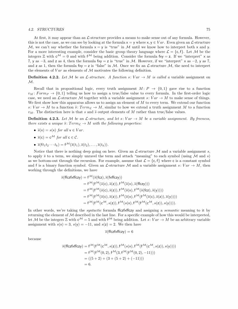
4.2. STRUCTURES 75
At first, it may appear than an L-structure provides a means to make sense out of any formula. However,this is not the case, as we can see by looking at the formula x = y where x, y ∈ V ar. Even given an L-structureM, we can’t say whether the formula x = y is “true” in M until we know how to interpret both x and y.For a more interesting example, consider the basic group theory language where L = {c, f}. Let M be theintegers Z with cM = 0 and with fM being addition. Consider the formula fxy = z. If we “interpret” x as7, y as −3, and z as 4, then the formula fxy = z is “true” in M. However, if we “interpret” x as −2, y as 7,and z as 1, then the formula fxy = z is “false” in M. Once we fix an L-structure M, the need to interpretthe elements of V ar as elements of M motivates the following definition.
Definition 4.2.2. Let M be an L-structure. A function s : V ar → M is called a variable assignment onM.
Recall that in propositional logic, every truth assignment M : P → {0, 1} gave rise to a functionvM : FormP → {0, 1} telling us how to assign a true/false value to every formula. In the first-order logiccase, we need an L-structure M together with a variable assignment s : V ar →M to make sense of things.We first show how this apparatus allows us to assign an element of M to every term. We extend our functions : V ar → M to a function s : TermL → M , similar to how we extend a truth assignment M to a functionvM . The distinction here is that s and s output elements of M rather than true/false values.
Definition 4.2.3. Let M be an L-structure, and let s : V ar → M be a variable assignment. By freeness,there exists a unique s : TermL →M with the following properties:
• s(x) = s(x) for all v ∈ V ar.
• s(c) = cM for all c ∈ C.
• s(ft1t2 · · · tk) = fM(s(t1), s(t2), . . . , s(tk)).
Notice that there is nothing deep going on here. Given an L-structure M and a variable assignment s,to apply s to a term, we simply unravel the term and attach “meaning” to each symbol (using M and s)as we bottom-out through the recursion. For example, assume that L = {c, f} where c is a constant symboland f is a binary function symbol. Given an L-structure M and a variable assignment s : V ar → M , thenworking through the definitions, we have
s(ffczfxffczy) = fM(s(fcz), s(fxffczy))
= fM(fM(s(c), s(z)), fM(s(x), s(ffczy)))
= fM(fM(s(c), s(z)), fM(s(x), fM(s(fcz), s(y))))
= fM(fM(s(c), s(z)), fM(s(x), fM(fM(s(c), s(z)), s(y))))
= fM(fM(cM, s(z)), fM(s(x), fM(fM(cM, s(z)), s(y)))).
In other words, we’re taking the syntactic formula ffczfxffczy and assigning a semantic meaning to it byreturning the element ofM described in the last line. For a specific example of how this would be interpreted,letM be the integers Z with cM = 5 and with fM being addition. Let s : V ar →M be an arbitrary variableassignment with s(x) = 3, s(y) = −11, and s(z) = 2. We then have
s(ffczfxffczy) = 6
because
s(ffczfxffczy) = fM(fM(cM, s(z)), fM(s(x), fM(fM(cM, s(z)), s(y))))
= fM(fM(0, 2), fM(3, fM(fM(0, 2),−11)))
= ((5 + 2) + (3 + (5 + 2) + (−11)))
= 6.
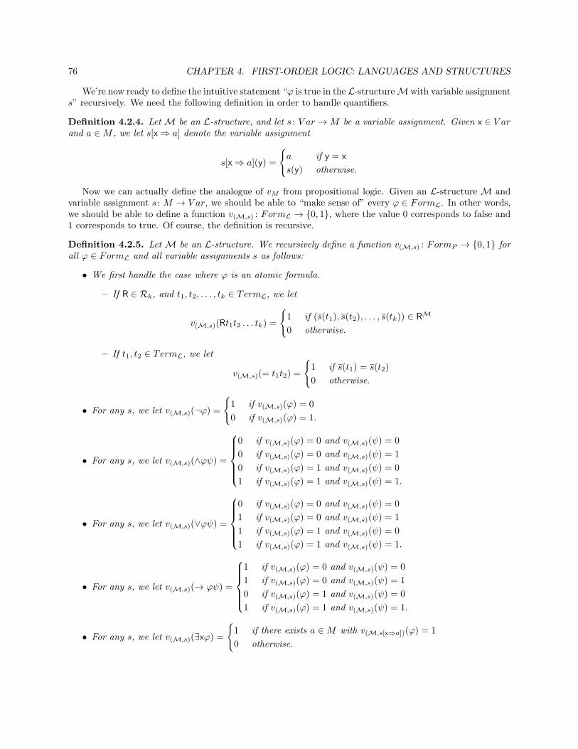
76 CHAPTER 4. FIRST-ORDER LOGIC: LANGUAGES AND STRUCTURES
We’re now ready to define the intuitive statement “ϕ is true in the L-structureM with variable assignments” recursively. We need the following definition in order to handle quantifiers.
Definition 4.2.4. Let M be an L-structure, and let s : V ar →M be a variable assignment. Given x ∈ V arand a ∈M , we let s[x⇒ a] denote the variable assignment
s[x⇒ a](y) =
{a if y = x
s(y) otherwise.
Now we can actually define the analogue of vM from propositional logic. Given an L-structure M andvariable assignment s : M → V ar, we should be able to “make sense of” every ϕ ∈ FormL. In other words,we should be able to define a function v(M,s) : FormL → {0, 1}, where the value 0 corresponds to false and1 corresponds to true. Of course, the definition is recursive.
Definition 4.2.5. Let M be an L-structure. We recursively define a function v(M,s) : FormP → {0, 1} forall ϕ ∈ FormL and all variable assignments s as follows:
• We first handle the case where ϕ is an atomic formula.
– If R ∈ Rk, and t1, t2, . . . , tk ∈ TermL, we let
v(M,s)(Rt1t2 . . . tk) =
{1 if (s(t1), s(t2), . . . , s(tk)) ∈ RM
0 otherwise.
– If t1, t2 ∈ TermL, we let
v(M,s)(= t1t2) =
{1 if s(t1) = s(t2)
0 otherwise.
• For any s, we let v(M,s)(¬ϕ) =
{1 if v(M,s)(ϕ) = 0
0 if v(M,s)(ϕ) = 1.
• For any s, we let v(M,s)(∧ϕψ) =
0 if v(M,s)(ϕ) = 0 and v(M,s)(ψ) = 0
0 if v(M,s)(ϕ) = 0 and v(M,s)(ψ) = 1
0 if v(M,s)(ϕ) = 1 and v(M,s)(ψ) = 0
1 if v(M,s)(ϕ) = 1 and v(M,s)(ψ) = 1.
• For any s, we let v(M,s)(∨ϕψ) =
0 if v(M,s)(ϕ) = 0 and v(M,s)(ψ) = 0
1 if v(M,s)(ϕ) = 0 and v(M,s)(ψ) = 1
1 if v(M,s)(ϕ) = 1 and v(M,s)(ψ) = 0
1 if v(M,s)(ϕ) = 1 and v(M,s)(ψ) = 1.
• For any s, we let v(M,s)(→ ϕψ) =
1 if v(M,s)(ϕ) = 0 and v(M,s)(ψ) = 0
1 if v(M,s)(ϕ) = 0 and v(M,s)(ψ) = 1
0 if v(M,s)(ϕ) = 1 and v(M,s)(ψ) = 0
1 if v(M,s)(ϕ) = 1 and v(M,s)(ψ) = 1.
• For any s, we let v(M,s)(∃xϕ) =
{1 if there exists a ∈M with v(M,s[x⇒a])(ϕ) = 1
0 otherwise.

4.2. STRUCTURES 77
• For any s, we let v(M,s)(∀xϕ) =
{1 for all a ∈M, we have v(M,s[x⇒a])(ϕ) = 1
0 otherwise.
The above recursive definition takes a little explanation, because some recursive “calls” change thevariable assignment. Thus, we are not fixing an L-structureM and a variable assignment s onM, and thendoing a recursive definition on ϕ ∈ FormL. To fit this recursive definition into our framework from Chapter2, we can adjust it as follows. Fix an L-structureM. Let V arAssignM be the set of all variable assignmentson M. We then define a function gM : FormP → V arAssignM recursively using the above rules as guides,with the intention that v(M,s)(ϕ) = 1 to mean that s ∈ gM(ϕ). Here are three representative examples ofhow we define gM:
gM(Rt1t2 . . . tk) = {s ∈ V arAssignM : (s(t1), s(t2), . . . , s(tk)) ∈ RM}gM(∧ϕψ) = gM(ϕ) ∩ gM(ψ)
gM(∃xϕ) =⋃a∈M{s ∈ V arAssignM : s[x⇒ a] ∈ gM(ϕ)}.
From here, we then define v(M,s)(ϕ) = 1 to mean that s ∈ gM(ϕ), and check that it has the requiredproperties.
Let’s consider a simple example. Let L = {R, f} where R is a unary relation symbol and f is a unaryfunction symbol. Let M be the following L-structure:
• M = {0, 1, 2, 3}.
• RM = {1, 3}.
• fM : M →M is the function defined by
fM(0) = 3 fM(1) = 1 fM(2) = 0 fM(3) = 3
We now explore the values of v(M,s)(ϕ) for various choices of variable assignments s and formulas ϕ.
1. Given any variable assignment s : V ar →M , we have
v(M,s)(¬Rx) = 1⇔ v(M,s)(Rx) = 0
⇔ s(x) /∈ RM
⇔ s(x) = 0 or s(x) = 2.
2. Given any variable assignment s : V ar →M , we have
v(M,s)(∃xRx) = 1⇔ There exists a ∈M such that v(M,s[x⇒a])(Rx) = 1
⇔ There exists a ∈M such that s[x⇒ a](x) ∈ RM
⇔ There exists a ∈M such that s[x⇒ a](x) ∈ RM
⇔ There exists a ∈M such that a ∈ RM.
Since RM 6= ∅, it follows that v(M,s)(∃xRx) = 1 for all variable assignments s : V ar →M .

78 CHAPTER 4. FIRST-ORDER LOGIC: LANGUAGES AND STRUCTURES
3. Given any variable assignment s : V ar →M , we have
v(M,s)(∀x(Rx→ (fx = x))) = 1⇔ For all a ∈M, we have v(M,s[x⇒a])((Rx→ (fx = x))) = 1
⇔ For all a ∈M, we have either
v(M,s[x⇒a])(Rx) = 0 or v(M,s[x⇒a])(fx = x) = 1
⇔ For all a ∈M, we have either
s[x⇒ a](x) /∈ RM or s[x⇒ a](fx) = s[x⇒ a](x)
⇔ For all a ∈M, we have either
s[x⇒ a](x) /∈ RM or fM(s[x⇒ a](x)) = s[x⇒ a](x)
⇔ For all a ∈M, we have either
s[x⇒ a](x) /∈ RM or fM(s[x⇒ a](x)) = s[x⇒ a](x)
⇔ For all a ∈M, we have either a /∈ RM or fM(a) = a.
Since 0 /∈ RM, fM(1) = 1, 2 /∈ RM, and fM(3) = 3, it follows that v(M,s)(∀x(Rx→ (fx = x))) = 1 forall variable assignments s : V ar →M .
In the above examples, notice that only the values of s on the free variables in ϕ affect whether or notv(M,s) = 1. In general, this seems intuitively clear, and we now state the corresponding precise result
Proposition 4.2.6. Let M be an L-structure.
1. Suppose that t ∈ TermL and s1, s2 : V ar → M are two variable assignments such that s1(x) = s2(x)for all x ∈ OccurV ar(t). We then have s1(t) = s2(t).
2. LetM be an L-structure. Suppose that ϕ ∈ FormL and s1, s2 : V ar →M are two variable assignmentssuch that s1(x) = s2(x) for all x ∈ FreeV ar(ϕ). We then have
v(M,s1)(ϕ) = 1 if and only if v(M,s2)(ϕ) = 1.
Proof. Each of these is a straightforward induction, the first on t ∈ TermL and the second on ϕ ∈ FormL.
We introduced the notation v(M,s)(ϕ) to correspond to our old notation vM (ϕ). In propositional logic,we need a truth assignment M : P → {0, 1} to assign true/false values to all formulas. In first-order logic,we need both an L-structure M and a variable assignment s : V ar → M to assign true/false values to allformulas. Despite the advantages of the similar notation, it is tiresome to keep writing so much in thesubscripts, and so people who work in mathematical logic have adopted other standard notation, which wenow introduce.
Notation 4.2.7. Let L be a language, let M be an L-structure, let s : V ar →M be a variable assignment,and let ϕ ∈ FormL. We write (M, s) � ϕ to mean that v(M,s)(ϕ) = 1, and write (M, s) 6� ϕ to mean thatv(M,s)(ϕ) = 0.
In some ways, using the symbol � is natural, because we are defining the semantic notion that ϕ is truein (M, s). However, in other ways, this notation is incredibly confusing. In propositional logic, we usedthe symbol � only in Γ � ϕ where Γ ⊆ FormP and ϕ ∈ FormP . In other words, we used � for semanticimplication, not semantic truth. Our new first-order logic notation would be akin to also writing M � ϕin propositional logic to mean that vM (ϕ) = 1. Although we could have done that in the Chapter 3, weavoided the temptation to overload the notation at that stage. We will eventually define Γ � ϕ in first-orderlogic when Γ ⊆ FormL and ϕ ∈ FormL, and at that point we will just have to know which version of � weare using based on what type of object appears on the left. Consider yourself warned!
With this new notation in hand, we can rewrite the recursive definition of v(M,s) in the following way:

4.2. STRUCTURES 79
• Suppose first that ϕ is an atomic formula.
– If ϕ is Rt1t2 · · · tk,, we have (M, s) � ϕ if and only if (s(t1), s(t2), . . . , s(tk)) ∈ RM.
– If ϕ is = t1t2, we have (M, s) � ϕ if and only if s(t1) = s(t2).
• For any s, we have (M, s) � ¬ϕ if and only if (M, s) 6� ϕ.
• For any s, we have (M, s) � ϕ ∧ ψ if and only if (M, s) � ϕ and (M, s) � ψ.
• For any s, we have (M, s) � ϕ ∨ ψ if and only if either (M, s) � ϕ or (M, s) � ψ.
• For any s, we have (M, s) � ϕ→ ψ if and only if either (M, s) 6� ϕ or (M, s) � ψ.
• For any s, we have (M, s) � ∃xϕ if and only if there exists a ∈M such that (M, s[x⇒ a]) � ϕ.
• For any s, we have (M, s) � ∀xϕ if and only if for all a ∈M , we have (M, s[x⇒ a]) � ϕ.
We now introduce some other notation in light of Proposition 4.2.6.
Notation 4.2.8. Let L be a language.
1. If x1, x2, . . . , xn ∈ V ar are distinct, and we refer to a formula ϕ(x1, x2, . . . , xn) ∈ FormL we mean thatϕ ∈ FormL and FreeV ar(ϕ) ⊆ {x1, x2, . . . , xn}.
2. Suppose that M is an L-structure, ϕ(x1, x2, . . . , xn) ∈ FormL, and a1, a2, . . . , an ∈ M . We write(M, a1, a2, . . . , an) � ϕ to mean that (M, s) � ϕ for some (any) s : V ar →M with s(xi) = ai for all i.
3. As a special case of 2, we have the following. Suppose that M is an L-structure and σ ∈ SentL. Wewrite M � σ to mean that (M, s) � σ for some (any) s : V ar →M .
As we’ve seen, given a language L, an L-structure can be any set M together with any interpretationof the symbols. In particular, although we might only have certain structures in mind when we describea language, the structures themselves need not respect our desires. However, since we have now formallydefined the intuitive notion that a sentence ϕ ∈ SentL is true in an L-structure M (recall that a sentencehas no free variables, so we don’t need a variable assignment), we now carve out classes of structures whichsatisfy certain sentences of our language.
Definition 4.2.9. Let L be a language, and let Σ ⊆ SentL. We let Mod(Σ) be the class of all L-structuresM such that M � σ for all σ ∈ Σ. If σ ∈ SentL, we write Mod(σ) instead of Mod({σ}).
Definition 4.2.10. Let L be a language and let K be a class of L-structures.
1. K is an elementary class if there exists σ ∈ SentL such that K = Mod(σ).
2. K is a weak elementary class if there exists Σ ⊆ SentL such that K = Mod(Σ).
By taking conjunctions, we have the following simple proposition.
Proposition 4.2.11. Let L be a language and let K be a class of L-structures. K is an elementary class ifand only if there exists a finite Σ ⊆ SentL such that K = Mod(Σ).
For example, let L = {R} where R is a binary relation symbol.
1. The class of partially ordered sets is an elementary class as we saw in Chapter 1, because we can let Σbe the following collection of sentences:
(a) ∀xRxx.
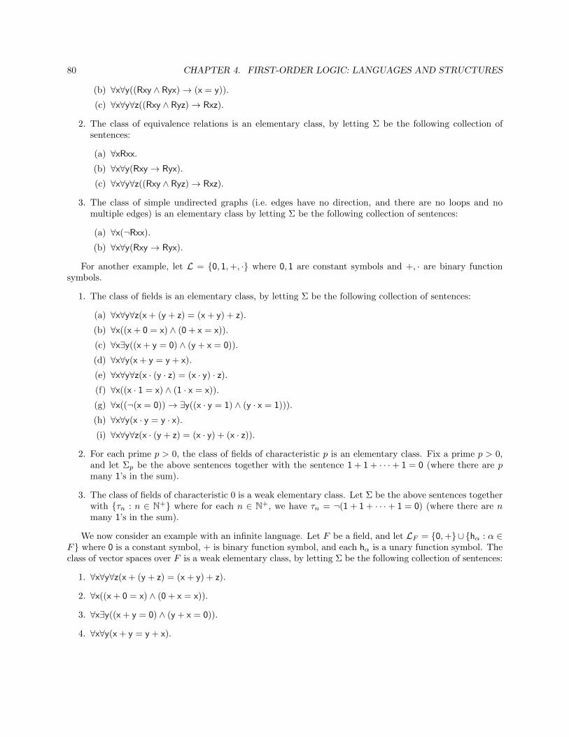
80 CHAPTER 4. FIRST-ORDER LOGIC: LANGUAGES AND STRUCTURES
(b) ∀x∀y((Rxy ∧ Ryx)→ (x = y)).
(c) ∀x∀y∀z((Rxy ∧ Ryz)→ Rxz).
2. The class of equivalence relations is an elementary class, by letting Σ be the following collection ofsentences:
(a) ∀xRxx.
(b) ∀x∀y(Rxy→ Ryx).
(c) ∀x∀y∀z((Rxy ∧ Ryz)→ Rxz).
3. The class of simple undirected graphs (i.e. edges have no direction, and there are no loops and nomultiple edges) is an elementary class by letting Σ be the following collection of sentences:
(a) ∀x(¬Rxx).
(b) ∀x∀y(Rxy→ Ryx).
For another example, let L = {0, 1,+, ·} where 0, 1 are constant symbols and +, · are binary functionsymbols.
1. The class of fields is an elementary class, by letting Σ be the following collection of sentences:
(a) ∀x∀y∀z(x + (y + z) = (x + y) + z).
(b) ∀x((x + 0 = x) ∧ (0 + x = x)).
(c) ∀x∃y((x + y = 0) ∧ (y + x = 0)).
(d) ∀x∀y(x + y = y + x).
(e) ∀x∀y∀z(x · (y · z) = (x · y) · z).
(f) ∀x((x · 1 = x) ∧ (1 · x = x)).
(g) ∀x((¬(x = 0))→ ∃y((x · y = 1) ∧ (y · x = 1))).
(h) ∀x∀y(x · y = y · x).
(i) ∀x∀y∀z(x · (y + z) = (x · y) + (x · z)).
2. For each prime p > 0, the class of fields of characteristic p is an elementary class. Fix a prime p > 0,and let Σp be the above sentences together with the sentence 1 + 1 + · · ·+ 1 = 0 (where there are pmany 1’s in the sum).
3. The class of fields of characteristic 0 is a weak elementary class. Let Σ be the above sentences togetherwith {τn : n ∈ N+} where for each n ∈ N+, we have τn = ¬(1 + 1 + · · ·+ 1 = 0) (where there are nmany 1’s in the sum).
We now consider an example with an infinite language. Let F be a field, and let LF = {0,+}∪{hα : α ∈F} where 0 is a constant symbol, + is binary function symbol, and each hα is a unary function symbol. Theclass of vector spaces over F is a weak elementary class, by letting Σ be the following collection of sentences:
1. ∀x∀y∀z(x + (y + z) = (x + y) + z).
2. ∀x((x + 0 = x) ∧ (0 + x = x)).
3. ∀x∃y((x + y = 0) ∧ (y + x = 0)).
4. ∀x∀y(x + y = y + x).

4.3. SUBSTRUCTURES AND HOMOMORPHISMS 81
5. ∀x∀y(hα(x + y) = hα(x) + hα(y)) for each α ∈ F .
6. ∀x(hα+β(x) = (hα(x) + hβ(x))) for each α, β ∈ F .
7. ∀x(hα·β(x) = hα(hβ(x))) for each α, β ∈ F .
8. ∀x(h1(x) = x).
Notice that if F is infinite, then we really have infinitely many formulas here, because three of the sentencesare parametrized by elements of F .
Finally, notice that given any language L and any n ∈ N+, the class of L-structures of cardinality atleast n is an elementary class as witnessed by the formula
∃x1∃x2 · · · ∃xn(∧
1≤i<j≤n
(xi 6= xj)).
Furthermore, the class of L-structures of cardinality equal to n is an elementary class. To see this, let σn bethe above formula for n, and consider the sentence σn ∧ (¬σn+1).
At this point, it’s often clear how to show that a certain class of structures is a (weak) elementary class:simply exhibit the correct sentences. However, it may seem very difficult to show that a class is not a (weak)elementary class. For example, is the class of fields of characteristic 0 an elementary class? Is the class offinite groups a weak elementary class? There are no obvious ways to answer these questions affirmatively.We’ll develop some tools later which will allow us to resolve these questions negatively.
Another interesting case is that of Dedekind-complete ordered fields. Now the ordered field axioms areeasily written down in the first-order language L = {0, 1,≤,+, ·}. In contrast, the Dedekind-completenessaxiom, which says that every nonempty subset which is bounded above has a least upper bound, can notbe directly translated in the language L because it involves quantifying over subsets instead of elements.However, we are unable to immediately conclude that this isn’t due to a lack of cleverness on our part.Perhaps there is an alternative approach which captures Dedekind-complete ordered fields in a first-orderway (by finding a clever equivalent first-order expression of Dedekind-completeness). More formally, theprecise question is whether the complete ordered fields are a (weak) elementary class in the language L.We’ll be able to answer this question in the negative later as well.
4.3 Substructures and Homomorphisms
One of the basic ways to obtain new algebraic structures (whether vector spaces, groups, or rings) is tofind them “inside” already established ones. For example, when working in the vector space of all functionsf : R → R under the usual pointwise operations, we can form the subspace of continuous functions, or thesubspace of differentiable functions. Within the symmetric groups Sn, one naturally defines the alternatinggroups An and dihedral groups Dn. These ideas also arise in combinatorial structures, such as when ex-amining subgraphs of a given graph, or viewing a partial ordering as a piece of a larger one. The generalunifying concept here is that of a substructure.
Definition 4.3.1. Let L be a language and let M and A be L-structures. We say that A is a substructureof M if the following conditions hold:
1. A ⊆M , where A and M are the underlying sets of A and M, respectively.
2. cA = cM for all c ∈ C.
3. RA = RM ∩Ak for all R ∈ Rk.
4. fA = fM � Ak for all f ∈ Fk.
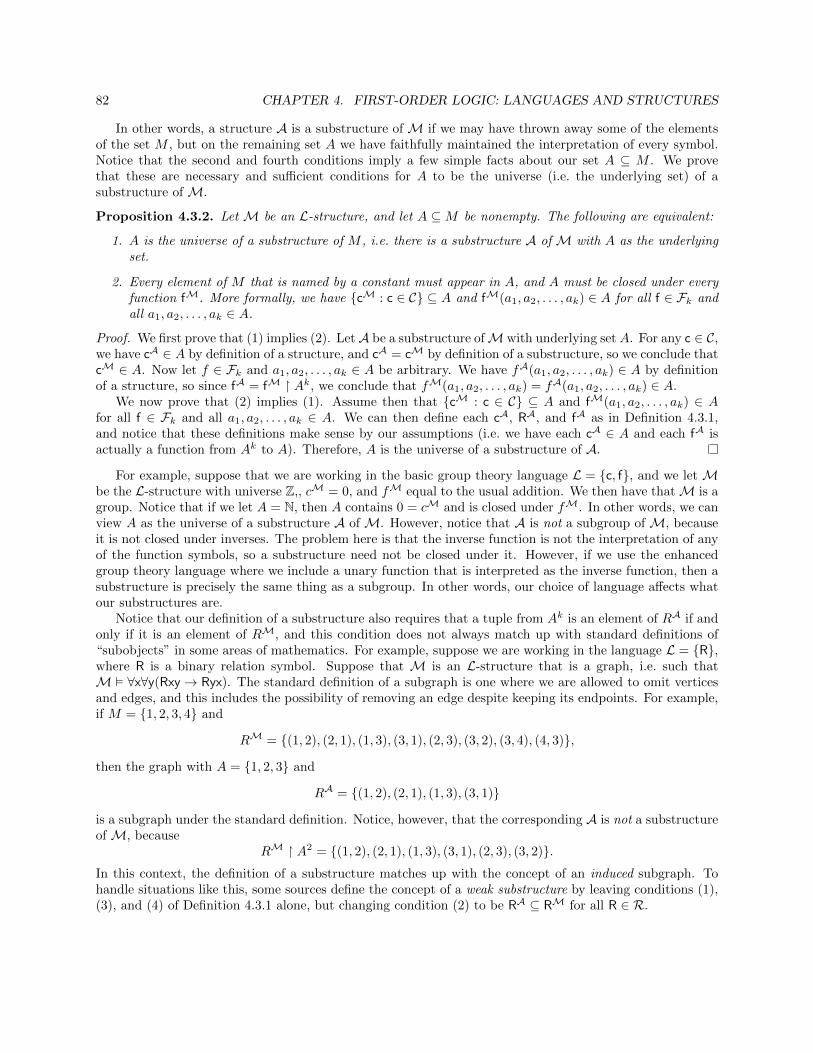
82 CHAPTER 4. FIRST-ORDER LOGIC: LANGUAGES AND STRUCTURES
In other words, a structure A is a substructure of M if we may have thrown away some of the elementsof the set M , but on the remaining set A we have faithfully maintained the interpretation of every symbol.Notice that the second and fourth conditions imply a few simple facts about our set A ⊆ M . We provethat these are necessary and sufficient conditions for A to be the universe (i.e. the underlying set) of asubstructure of M.
Proposition 4.3.2. Let M be an L-structure, and let A ⊆M be nonempty. The following are equivalent:
1. A is the universe of a substructure of M , i.e. there is a substructure A of M with A as the underlyingset.
2. Every element of M that is named by a constant must appear in A, and A must be closed under everyfunction fM. More formally, we have {cM : c ∈ C} ⊆ A and fM(a1, a2, . . . , ak) ∈ A for all f ∈ Fk andall a1, a2, . . . , ak ∈ A.
Proof. We first prove that (1) implies (2). LetA be a substructure ofM with underlying set A. For any c ∈ C,we have cA ∈ A by definition of a structure, and cA = cM by definition of a substructure, so we conclude thatcM ∈ A. Now let f ∈ Fk and a1, a2, . . . , ak ∈ A be arbitrary. We have fA(a1, a2, . . . , ak) ∈ A by definitionof a structure, so since fA = fM � Ak, we conclude that fM(a1, a2, . . . , ak) = fA(a1, a2, . . . , ak) ∈ A.
We now prove that (2) implies (1). Assume then that {cM : c ∈ C} ⊆ A and fM(a1, a2, . . . , ak) ∈ Afor all f ∈ Fk and all a1, a2, . . . , ak ∈ A. We can then define each cA, RA, and fA as in Definition 4.3.1,and notice that these definitions make sense by our assumptions (i.e. we have each cA ∈ A and each fA isactually a function from Ak to A). Therefore, A is the universe of a substructure of A.
For example, suppose that we are working in the basic group theory language L = {c, f}, and we let Mbe the L-structure with universe Z,, cM = 0, and fM equal to the usual addition. We then have thatM is agroup. Notice that if we let A = N, then A contains 0 = cM and is closed under fM. In other words, we canview A as the universe of a substructure A of M. However, notice that A is not a subgroup of M, becauseit is not closed under inverses. The problem here is that the inverse function is not the interpretation of anyof the function symbols, so a substructure need not be closed under it. However, if we use the enhancedgroup theory language where we include a unary function that is interpreted as the inverse function, then asubstructure is precisely the same thing as a subgroup. In other words, our choice of language affects whatour substructures are.
Notice that our definition of a substructure also requires that a tuple from Ak is an element of RA if andonly if it is an element of RM, and this condition does not always match up with standard definitions of“subobjects” in some areas of mathematics. For example, suppose we are working in the language L = {R},where R is a binary relation symbol. Suppose that M is an L-structure that is a graph, i.e. such thatM � ∀x∀y(Rxy→ Ryx). The standard definition of a subgraph is one where we are allowed to omit verticesand edges, and this includes the possibility of removing an edge despite keeping its endpoints. For example,if M = {1, 2, 3, 4} and
RM = {(1, 2), (2, 1), (1, 3), (3, 1), (2, 3), (3, 2), (3, 4), (4, 3)},
then the graph with A = {1, 2, 3} and
RA = {(1, 2), (2, 1), (1, 3), (3, 1)}
is a subgraph under the standard definition. Notice, however, that the corresponding A is not a substructureof M, because
RM � A2 = {(1, 2), (2, 1), (1, 3), (3, 1), (2, 3), (3, 2)}.In this context, the definition of a substructure matches up with the concept of an induced subgraph. Tohandle situations like this, some sources define the concept of a weak substructure by leaving conditions (1),(3), and (4) of Definition 4.3.1 alone, but changing condition (2) to be RA ⊆ RM for all R ∈ R.

4.3. SUBSTRUCTURES AND HOMOMORPHISMS 83
Suppose that we have a structureM, and we have an arbitrary set B ⊆M . How can we get a substructureA of M such that B ⊆ A? By Proposition 4.3.2, we need to ensure that A contains both B and theinterpretation of the constants, and is closed under the functions fM. Thus, we can build a substructure (infact the smallest substructure containing B) by starting with B and the various cM, and then generatingnew elements. In other words, we have the following result. Notice that we need to assume that either B 6= ∅or C 6= ∅ so that we start with a nonempty set, since we require that A 6= ∅.
Corollary 4.3.3. Let M be an L-structure and let B ⊆ M be an arbitrary set. Suppose either that B 6= ∅or C 6= ∅. If we let A = G(M,B ∪ {cM : c ∈ C}, {fM : f ∈ F}), then A is the universe of a substructure ofM. Moreover, if N is any substructure of M with B ⊆ N , then A ⊆ N .
We now seek to generalize the concept of a homomorphisms from their algebra roots to more generalstructures. In group theory, a homomorphism is an function that preserves the only binary operation. Inthis setting, it is straightforward to check that a group homomorphism automatically sends the identityto the identity. For rings with identity, it is possible to have a function that preserves both addition andmultiplication, but not the multiplicative identity. As a result, some sources enforce the additional conditionthat a ring homomorphism must also preserve the multiplicative identity. In first-order logic, we requirethat the interpretation of the all of the first-order symbols in L is preserved. In other words, if we chooseto include a constant symbol for the multiplicative identity in our language, then the multiplicative identityof the first ring must be sent to the multiplicative identity of the second. Thus, as with substructures, ourchoice of language will affect what functions we call homomorphisms.
Definition 4.3.4. Let L be a language, and let M and N be L-structures.
1. A function h : M → N is called a homomorphism if it satisfies the following conditions:
(a) For all c ∈ C, we have h(cM) = cN .
(b) For all R ∈ Rk and all a1, a2, . . . , ak ∈M , we have
(a1, a2, . . . , ak) ∈ RM if and only if (h(a1), h(a2), . . . , h(ak)) ∈ RN .
(c) For all f ∈ Fk and all a1, a2, . . . , ak ∈M , we have
h(fM(a1, a2, . . . , ak)) = fN (h(a1), h(a2), . . . , h(ak)).
2. A function h : M → N is called an embedding if it is an injective homomorphism.
3. A function h : M → N is called an isomorphism if it is a bijective homomorphism.
We now jump into our primary theorem about homomorphisms and isomorphisms. The last part of thistheorem gives one precise way to say that all “reasonable” properties are preserved by an isomorphism. It’snot an at all clear how to make this precise in algebra, but now we have a formal language that allowsus to codify (at least some) “reasonable” properties. Since first-order formulas are generated from atomicformulas using simple rules, we can prove by induction that all properties expressible by first-order formulasare preserved.
Theorem 4.3.5. Let L be a language, and let M and N be L-structures. Suppose that h : M → N is ahomomorphism, and suppose that s : V ar →M is a variable assignment. We have the following.
1. The function h ◦ s is a variable assignment on N .
2. For any t ∈ TermL, we have h(s(t)) = h ◦ s(t).

84 CHAPTER 4. FIRST-ORDER LOGIC: LANGUAGES AND STRUCTURES
3. For every quantifier-free ϕ ∈ FormL not containing the equality symbol, i.e. for all ϕ generated bystarting only with atomic formulas using elements of R, and generating with just the propositionalconnectives, we have
(M, s) � ϕ if and only if (N , h ◦ s) � ϕ.
4. If h is an embedding, then for every quantifier-free ϕ ∈ FormL, i.e. for all ϕ generated by startingwith all atomic formulas and using just the propositional connectives, we have
(M, s) � ϕ if and only if (N , h ◦ s) � ϕ.
5. If h is an isomorphism, then for every ϕ ∈ FormL, we have
(M, s) � ϕ if and only if (N , h ◦ s) � ϕ.
Proof.
1. This is immediate from the fact that s : V ar →M and h : M → N , so h ◦ s : V ar → N .
2. The proof is by induction on t. We have two base cases. For any c ∈ C, we have
h(s(c)) = h(cM)
= cN (since h is a homomorphism)
= h ◦ s(c).
Also, for any x ∈ V ar, we have
h(s(x)) = h(s(x))
= (h ◦ s)(x)
= h ◦ s(x).
For the inductive step, let f ∈ Fk and let t1, t2, . . . , tk ∈ TermL be such that the statement is true foreach ti. We then have
h(s(ft1t2 · · · tk)) = h(fM(s(t1), s(t2), . . . , s(tk))) (by definition of s)
= fM(h(s(t1)), h(s(t2)), . . . , h(s(tk))) (since h is a homomorphism)
= fN (h ◦ s(t1), h ◦ s(t2), . . . , h ◦ s(tk)) (by induction)
= h ◦ s(ft1t2 · · · tk) (by definition of h ◦ s).
Hence, the statement is true for ft1t2 · · · tk, which completes the induction.
3. Assume that h is an embedding. The proof is by induction ϕ. Let R ∈ Rk and t1, t2, . . . , tk ∈ TermLbe arbitrary. We have
(M, s) � Rt1t2 · · · tk ⇔ (s(t1), s(t2), . . . , s(tk)) ∈ RM
⇔ (h(s(t1)), h(s(t2)), . . . , h(s(tk))) ∈ RN (since h is a homomorphism)
⇔ (h ◦ s(t1), h ◦ s(t2), . . . , h ◦ s(tk)) ∈ RN (by part 1)
⇔ (N , h ◦ s) � Rt1t2 · · · tk.

4.3. SUBSTRUCTURES AND HOMOMORPHISMS 85
Suppose that the result holds for ϕ. We prove it for ¬ϕ. We have
(M, s) � ¬ϕ⇔ (M, s) 6� ϕ⇔ (N , h ◦ s) 6� ϕ (by induction)
⇔ (N , h ◦ s) � ¬ϕ.
Suppose that the result holds for ϕ and ψ. We have
(M, s) � ϕ ∧ ψ ⇔ (M, s) � ϕ and (M, s) � ψ
⇔ (N , h ◦ s) � ϕ and (N , h ◦ s) � ϕ (by induction)
⇔ (N , h ◦ s) � ϕ ∧ ψ,
and similarly for ∨ and →. The result follows by induction.
4. In light of the proof of (3), we need only show that if ϕ is = t1t2 where t1, t2 ∈ TermL, then (M, s) � ϕif and only if (N , h ◦ s) � ϕ. For any t1, t2 ∈ TermL, we have
(M, s) � = t1t2 ⇔ s(t1) = s(t2)
⇔ h(s(t1)) = h(s(t2)) (since h is injective)
⇔ h ◦ s(t1) = h ◦ s(t2) (by part 1)
⇔ (N , h ◦ s) � = t1t2.
5. Suppose that the result holds for ϕ and x ∈ V ar. We have
(M, s) � ∃xϕ⇔ There exists a ∈M such that (M, s[x⇒ a]) � ϕ
⇔ There exists a ∈M such that (N , h ◦ (s[x⇒ a])) � ϕ (by induction)
⇔ There exists a ∈M such that (N , (h ◦ s)[x⇒ h(a)] � ϕ
⇔ There exists b ∈ N such that (N , (h ◦ s)[x⇒ b]) � ϕ (since h is bijective)
⇔ (N , h ◦ s) � ∃xϕ,
and also
(M, s) � ∀xϕ⇔ For all a ∈M , we have (M, s[x⇒ a]) � ϕ
⇔ For all a ∈M , we have (N , h ◦ (s[x⇒ a])) � ϕ (by induction)
⇔ For all a ∈M , we have (N , (h ◦ s)[x⇒ h(a)]) � ϕ
⇔ For all b ∈ N , we have (N , (h ◦ s)[x⇒ b]) � ϕ (since h is bijective)
⇔ (N , h ◦ s) � ∀xϕ.
Definition 4.3.6. Let M and N be L-structures. We say that M and N are isomorphic if there exists anisomorphism h : M→N . In this case, we write M∼= N .
We now introduce one of the central definitions of logic.
Definition 4.3.7. Let L be a language, and let M and N be L-structures. We write M≡ N , and say thatM and N are elementarily equivalent, if for all σ ∈ SentL, we have M � σ if and only if N � σ.

86 CHAPTER 4. FIRST-ORDER LOGIC: LANGUAGES AND STRUCTURES
In other words, two structures are elementarily equivalent if the same sentences are true in each structure.Notice that, by Proposition 4.2.6 we do not need to include any variable assignments in our definition, sincesentences do not have free variables. The fact that a given sentence can be evaluated to a true/false valuewithout a variable assignment is precisely what allows us to compare sentences across structures with perhapsvery different underlying sets.
Corollary 4.3.8. Let L be a language, and let M and N be L-structures. If M∼= N , then M≡ N .
Proof. Let M and N be L-structures, and assume that M ∼= N . Fix an isomorphism h : M → N . Letσ ∈ SentL be arbitrary. Fix some (any) variable assignment on M . By Theorem 4.3.5, we have
(M, s) � σ if and only if (N , h ◦ s) � σ.
Now since σ has no free variables, the variable assignments don’t matter (see Notation 4.2.8), so we concludethat M � σ if and only if N � σ. Since σ ∈ SentL was arbitrary, it follows that M≡ N .
Somewhat surprisingly, the converse of Corollary 4.3.8 is not true. In other words, there are elementarilyequivalent structures that are not isomorphic. In fact, not only do such examples exist, but we will seethat for essentially every structure M, we can build a structure N with M ≡ N but M 6∼= N . Beyondhow intrinsically amazing this is, it turns out to be useful. If we want to show that M � σ for a givenσ ∈ SentL, we can think about going to an elementarily equivalent structure N that is easier to work withor understand, and show that N � σ. We will eventually see some extraordinary examples of arguments inthis style.
Returning to substructures, notice that if A is a substructure ofM, then we typically have A 6≡ M. Forexample, it’s possible that a subgroup of a nonabelian group is abelian. For example, if M is the group S3,and A is the substructure of M with underlying set {id, (1 2)} (where id is the identity function), then wehave
M 6� ∀x∀y(f(x, y) = f(y, x))
butA � ∀x∀y(f(x, y) = f(y, x)).
Nonetheless, there are connections between when some restricted types of formulas are true in A versus inM. To see this, we start with the following simple remark.
Proposition 4.3.9. Let L be a language and letM and A be L-structures with A ⊆M . We then have that Ais a substructure of M if and only if the inclusion function i : A→M given by i(a) = a is a homomorphism.
Proof. Immediate from the corresponding definitions.
Definition 4.3.10. Let L be a language, and let QuantFreeFormL be the set of all quantifier-free formulas.
1. A Σ1 formula is an element of G(Sym∗L, QuantFreeFormL, {h∃,x : x ∈ V ar}).
2. A Π1 formula is an element of G(Sym∗L, QuantFreeFormL, {h∀,x : x ∈ V ar}).
In other words, a Σ1 formula is a formula that begins with a block of existential quantifiers, and thenis followed by a quantifier-free formula. A Π1 formula instead begins with a block of universal quantifiers,followed by a quantifier-free formula. For example,
∀x∀y(f(x, y) = f(y, x))
is a Π1 formula in the language of group theory. We can now state and prove some simple connectionsbetween how the truth of these formulas can vary between a substructure and the bigger structure.

4.4. DEFINABILITY 87
Proposition 4.3.11. Suppose that A ⊆M.
1. For any quantifier-free formula ϕ and any s : V ar → A, we have
(A, s) � ϕ if and only if (M, s) � ϕ.
2. For any Σ1 formula ϕ and any s : V ar → A, we have
If (A, s) � ϕ, then (M, s) � ϕ.
3. For any Π1 formula ϕ and any s : V ar → A, we have
If (M, s) � ϕ, then (A, s) � ϕ.
Proof.
1. This follows from Proposition 4.3.9 and Theorem 4.3.5, using the embedding i (since i ◦ s = s).
2. We prove this by induction. If ϕ is quantifier-free, the part (1) can be directly applied. Suppose thatwe know the result for ϕ, and suppose that (A, s) � ∃xϕ. By definition, we can fix a ∈ A such that(A, s[x⇒ a]) � ϕ. By induction, we know that (M, s[x⇒ a]) � ϕ, hence (M, s) � ∃xϕ.
3. We prove this by induction. If ϕ is quantifier-free, the part (1) can be directly applied. Suppose thatwe know the result for ϕ, and suppose that (M, s) � ∀xϕ. By definition, we know that for everya ∈ A, we then have (M, s[x ⇒ a]) � ϕ, and hence (A, s[x ⇒ a]) � ϕ by induction. It follows that(A, s) � ∀xϕ.
For example, the sentence σ equal to ∀x∀y(f(x, y) = f(y, x)) is a Π1 formula. If M is a structure withM � σ, then whenever A is a substructure of M, we have that A � σ. In particular, every subgroup of anabelian group is abelian. As mentioned above, the converse does not hold, and this is the reason why weonly have one direction in Proposition 4.3.11 in the case of Σ1 and Π1 formulas.
For more complicated formulas, we may not be able to go in either direction. For example, consider thelanguage L = {0, 1,+, ·} of ring theory. Let σ be the sentence
∀x(¬(x = 0)→ ∃y(x · y = 1)),
which says that every nonzero element has a multiplicative inverse. Notice that σ is neither a Σ1 formulanor a Π1 formula. Now if we consider the L-structure M consisting of the rational field and let A be thesubstructure consisting of the integers, then M � σ but A 6� σ. In contrast, if we consider the L-structureM consisting of the polynomial ring R[x] and let A be the substructure consisting of the real numbers(i.e. constant polynomials), then M 6� σ but A � σ. In other words, if a formula is neither Σ1 nor Π1, it ispossible that the truth of the formula in a structure has no relation to its truth in a substructure.
4.4 Definability
A wonderful side-effect of developing a formal language is the ability to talk about what objects we candefine using that language.
Definition 4.4.1. Let M be an L-structure, let k ∈ N+, and let X ⊆ Mk. We say that X is definable inM if there exists ϕ(x1, x2, . . . , xk) ∈ FormL such that
X = {(a1, a2, . . . , ak) ∈Mk : (M, a1, a2, . . . , ak) � ϕ}.

88 CHAPTER 4. FIRST-ORDER LOGIC: LANGUAGES AND STRUCTURES
In other words, a set X ⊆Mk is definable inM if we can find a formula ϕ with k free variables such thatthe formula is true in M when when interpret the free variables as a k-tuple in X, and is false otherwise.For example, let L = {0, 1,+, ·} be the language of ring theory, where 0 and 1 are constant symbols and +and · are binary function symbols.
1. The set X = {(m,n) ∈ N2 : m < n} is definable in the structure (N, 0, 1,+, ·) as witnessed by theformula
∃z(z 6= 0 ∧ (x + z = y)).
2. The set X = {n ∈ N : n is prime} is definable in the structure (N, 0, 1,+, ·) as witnessed by the formula
¬(x = 1) ∧ ∀y∀z(x = y · z→ (y = 1 ∨ z = 1)).
3. The set X = {r ∈ R : r ≥ 0} is definable in the structure (R, 0, 1,+, ·) as witnessed by the formula
∃y(y · y = x).
Let’s consider another language. Let L = {<} where < is a binary relation symbol. For every n ∈ N,the set {n} is definable in (N, <). To see this, for each nN+, let ϕn(x) be the formula
∃y1∃y2 · · · ∃yn(∧
1≤i<j≤n
(yi 6= yj) ∧n∧
i=1
(yi < x)).
For each n ∈ N+, the formula ϕn(x) defines the set {k ∈ N : n ≤ k}. Now notice that {0} is definable aswitnessed by the formula
¬∃y(y < x),
and for each n ∈ N+, the set {n} is definable as witnessed by the formula
ϕn(x) ∧ ¬ϕn+1(x).
Finally, let L = {e, f} be the basic group theory language. Let (G, e, ·) be a group interpreted as anL-structure. The center of G is definable in (G, e, ·) as witnessed by the formula
∀y(f(x, y) = f(y, x))
Sometimes, there isn’t an obvious way to show that a set is definable, but some cleverness and/ornontrivial mathematics comes to the rescue. In each of the examples below, let L = {0, 1,+, ·} be thelanguage of ring theory.
1. The set N is definable in (Z, 0, 1,+, ·) as witnessed by the formula
∃y1∃y2∃y3∃y4(x = y1 · y1 + y2 · y2 + y3 · y3 + y4 · y4)
Certainly every element of Z that is a sum of squares must be an element of N. The fact that everyelement of N is a sum of four squares is Lagrange’s Theorem, an important result in number theory.
2. Let (R, 0, 1,+, ·) be a commutative ring. The Jacobson radical of R, denoted Jac(R) is the intersectionof all maximal ideal of R. As stated, it is not clear that this is definable in (R, 0, 1,+, ·) because itappears to quantify over subsets. However, a basic result in commutative algebra says that
a ∈ Jac(R)⇐⇒ ab− 1 is a unit for all b ∈ R⇐⇒ For all b ∈ R, there exists c ∈ R with (ab− 1)c = 1.
Using this, it follows that Jac(R) is definable in (R, 0, 1,+, ·) as witnessed by the formula
∀y∃z((x · y) · z = z + 1).

4.4. DEFINABILITY 89
3. The set Z is definable in (Q, 0, 1,+, ·). This is a deep result of Julia Robinson using some nontrivialnumber theory.
4. The set X = {(k,m, n) ∈ N3 : km = n} is definable in (N, 0, 1,+, ·), as is the set
{(m,n) ∈ N2 : m is the nth digit in the decimal expansion of π}.
In fact, every set C ⊆ Nk which is “computable” (i.e. for which it is possible to write a computerprogram that outputs yes on elements of C and no on elements of Nk\C) is definable in (N, 0, 1,+, ·).We will prove this challenging, but fundamental, result later.
The collection of definable sets in a structure have some simple closure properties.
Proposition 4.4.2. Let M be an L-structure, and let k ∈ N+. Let
Dk = {X ∈ P(Mk) : X is definable in M}.
We have the following:
1. If X,Y ∈ Dk, then X ∪ Y ∈ Dk.
2. If X,Y ∈ Dk, then X ∩ Y ∈ Dk.
3. If X ∈ Dk, then M\X ∈ Dk.
Proof. Each of these follow by taking the ∨, ∧, and ¬ of the respective formulas.
Determining which sets in a structure are definable is typically a challenging task, but classifying thecollection of definable sets is one of the primary goals when seeking to fully “understand” a structure. Let’sreturn to the language L = {0, 1,+, ·} of ring theory. Here we outline several important restrictions ondefinable sets in a few natural L-structures. We will prove each of these facts later.
1. In the structure (C, 0, 1,+, ·), every subset of C that is definable is either finite or cofinite (i.e. itscomplement is finite). The converse is not true. For example, any element of C that is transcendentalover Q is not an element of any finite definable set.
2. In the structure (R, 0, 1,+, ·), every subset of R that is definable is a finite union of intervals and points(but again, the converse is not true).
3. In the structure (N, 0, 1,+, ·), every computable subset of N is definable. In fact, many other subsetsof Z are also definable, and it is challenging to describe a subset of N that is not definable (althoughwe will eventually do this).
4. Since N is definable in (Z, 0, 1,+, ·), it turns out that the definable subsets of Z are also rich andcomplicated.
5. Since Z is definable in (Q, 0, 1,+, ·), the definable subsets of Q are similarly complicated.
As for elementary classes, it’s clear how to attempt to show that something is definable (although aswe’ve seen this may require a great deal of cleverness). However, it’s not at all obvious how one could showthat a set is not definable. Fortunately, Theorem 4.3.5 can be used to prove negative results.
Definition 4.4.3. Let M be an L-structure. An isomorphism h : M →M is called an automorphism.
Proposition 4.4.4. Suppose that M is an L-structure and k ∈ N+. Suppose also that X ⊆Mk is definablein M and that h : M →M is an automorphism. For every a1, a2, . . . , ak ∈M , we have
(a1, a2, . . . , ak) ∈ X if and only if (h(a1), h(a2), . . . , h(ak)) ∈ X.

90 CHAPTER 4. FIRST-ORDER LOGIC: LANGUAGES AND STRUCTURES
Proof. Fix ϕ(x1, x2, . . . , xk) ∈ FormL such that
X = {(a1, a2, . . . , ak) ∈Mk : (M, a1, a2, . . . , ak) � ϕ}.
By part 4 of Theorem 4.3.5, we know that for every a1, a2, . . . , ak ∈M , we have
(M, a1, a2, . . . , ak) � ϕ if and only if (M, h(a1), h(a2), . . . , h(ak)) � ϕ.
Therefore, for every a1, a2, . . . , ak ∈M , we have
(a1, a2, . . . , ak) ∈ X if and only if (h(a1), h(a2), . . . , h(ak)) ∈ X.
In other words, automorphisms of a structure must fix definable sets as a whole (note that this is notsaying must fix definable sets pointwise). Therefore, in order to show that a given set is not definable, wecan find an automorphism that does not fix the set.
Corollary 4.4.5. Suppose that M is an L-structure and k ∈ N+. Suppose also that X ⊆ Mk and thath : M → M is an automorphism. Suppose that there exists a1, a2, . . . , ak ∈ M such that exactly one of thefollowing holds:
• (a1, a2, . . . , ak) ∈ X.
• (h(a1), h(a2), . . . , h(ak)) ∈ X.
We then have that X is not definable in M.
For example, let L = {R} where R is a binary relation symbol, and let M be the L-structure whereM = Z and RM = {(a, b) ∈ Z2 : a < b}. We show that a set X ⊆ M is definable in M if and only if eitherX = ∅ or X = Z. First notice that ∅ is definable as witnessed by ¬(x = x) and Z as witnessed by x = x.Suppose now that X ⊆ Z is such that X 6= ∅ and X 6= Z. Fix a, b ∈ Z such that a ∈ X and b /∈ X. Defineh : M → M by letting h(c) = c + (b − a) for all c ∈ M . Notice that h is automorphism of M because it isbijective (the map g(c) = c− (b− a) is clearly an inverse) and a homomorphism. For the latter, notice thatif c1, c2 ∈ Z are arbitrary, then have have
(c1, c2) ∈ RM ⇔ c1 < c2
⇔ c1 + (b− a) < c2 + (b− a)
⇔ h(c1) < h(c2)
⇔ (h(c1), h(c2)) ∈ RM.
Notice also that h(a) = a+ (b− a) = b, so a ∈ X but h(a) /∈ X. Using Corollary 4.4.5, it follows that X isnot definable in M.
Definition 4.4.6. LetM be an L-structure. Suppose that k ∈ N+ and X ⊆Mk. We say that X is definablewith parameters inM if there exists ϕ(x1, x2, . . . , xk, y1, y2, . . . , yn) ∈ FormL together with b1, b2, . . . , bn ∈Msuch that
X = {(a1, a2, . . . , ak) ∈Mk : (M, a1, a2, . . . , ak, b1, b2, . . . , bn) � ϕ}
Intuitively, this means that we use elements of M inside our formulas to help us define sets. For example,for each n ∈ Z the set {n} is trivially definable with parameters in the structure M = (Z, <): simply letϕ(x, y) be the formula x = y, and notice that for each a ∈ Z, we have
(M, a, n) � ϕ⇔ a = n.
4.5. ELEMENTARY SUBSTRUCTURES 91
In fact, given any structure M, the set {m} is definable with parameters in M.Let’s return to the language L = {0, 1,+, ·}. Above, we talked about restrictions on definable sets in
several natural L-structures. We now discuss the situation when we switch to looking at those sets that aredefinable with parameters.
1. In the structure (C, 0, 1,+, ·), a subset of C is definable with parameters if and only if it is either finiteor cofinite.
2. In the structure (R, 0, 1,+, ·), a subset of R is definable with parameters if and only if it is finite unionof intervals and points.
3. In the structures with underlying sets N, Z, and Q, we can already define each specific element withoutparameters, so it turns out that a set is definable with parameters if and only if it is definable.
4.5 Elementary Substructures
Suppose that A is a substructure ofM. In Proposition 4.3.11, we showed that for all quantifier-free formulasϕ and all s : V ar → A, we have
(A, s) � ϕ if and only if (M, s) � ϕ.
Once we look at more general formulas involving quantifiers, this connection can easily break down. After all,a quantifier ranges over the entire underlying set, so if A is a proper subset of M , the recursive definitions of �will greatly differ. Regardless, it is at least conceivable that a proper substructure of a larger structure mightoccasionally satisfy the same formulas. We give these (at the moment seemingly magical) substructures aspecial name.
Definition 4.5.1. Let L be a language, let M be an L-structure, and let A be a substructure of M. We saythat A is an elementary substructure if for all ϕ ∈ FormL and all s : V ar → A, we have
(A, s) � ϕ if and only if (M, s) � ϕ.
We write A �M to mean that A is an elementary substructure of M.
Notice that if A is an elementary substructure ofM, then in particular we have that A ≡M, i.e. that Ais elementarily equivalent to M. To see this, simply notice that every σ ∈ SentL is in particular a formula,and that variable assignments do not affect the truth of sentences (since sentences have no free variables).
However, it is possible that to have a substructure A ofM with A ≡M, but where A 6� M. For example,let L = {f} where f is a unary function symbol. LetM be the L-structure with M = N and fM(n) = n+ 1.Let A be L-structure with A = N+ and fA(n) = n+ 1. We then have that A is a substructure of M. NowA ∼=M via the function h(m) = m−1, so A ≡M by Corollary 4.3.8. However, notice that A 6� M becauseif ϕ(x) is the formula ∃y(fy = x), we then have that (A, 1) 6� ϕ but (M, 1) � ϕ. Generalizing this example,one can show that the only elementary substructure of M is the structure M itself (noting that A has tohave a smallest element by well-ordering, then using the above argument to argue that this smallest elementis 0, and finally using the fact that A must be closed under the successor function).
Before jumping into a result that will greatly simplify the construction of elementary substructures, westart with a simple lemma that will allow us to turn one type of quantifier into the other.
Lemma 4.5.2. Let M be an L-structure, and let s : V ar → M be a variable assignment. For any ϕ ∈FormL, we have
(M, s) � ∀xϕ if and only if (M, s) � ¬∃x¬ϕ.

92 CHAPTER 4. FIRST-ORDER LOGIC: LANGUAGES AND STRUCTURES
Proof. Let ϕ ∈ FormL be arbitrary. Using the recursive definition of �, we have
(M, s) � ∀xϕ⇔ For all a ∈M, we have (M, s[x⇒ a]) � ϕ
⇔ For all a ∈M, we have (M, s[x⇒ a]) 6� ¬ϕ⇔ There does not exist a ∈M with (M, s[x⇒ a]) � ¬ϕ⇔ (M, s) 6� ∃x¬ϕ⇔ (M, s) � ¬∃x¬ϕ.
As mentioned above, the quantifiers are the obstacle in pushing Proposition 4.3.11 from simple formulasto more complex ones. The next test simplifies the process to that of checking one existential quantifier ata time. Notice that the condition it provides is only about truth in the structure M, and hence does notreference truth in A.
Theorem 4.5.3 (Tarski-Vaught Test). Suppose that A is a substructure ofM. The following are equivalent:
1. A �M, i.e. A is an elementary substructure of M.
2. Whenever ϕ ∈ FormL, x ∈ V ar, and s : V ar → A satisfy (M, s) � ∃xϕ, there exists a ∈ A such that
(M, s[x⇒ a]) � ϕ.
Proof. We first prove that 1 implies 2. Suppose then that A � M. Let ϕ ∈ FormL and s : V ar → A bearbitrary such that (M, s) � ∃xϕ. Using the fact that A �M, it follows that (A, s) � ∃xϕ. Fix a ∈ A suchthat (A, s[x⇒ a]) � ϕ. Using again the fact that A �M, we have (M, s[x⇒ a]) � ϕ.
We now prove that 2 implies 1. We prove by induction on ϕ ∈ FormL that for all s : V ar → A, we have(A, s) � ϕ if and only if (M, s) � ϕ. That is, we let
X = {ϕ ∈ FormL : For all s : V ar → A we have (A, s) � ϕ if and only if (M, s) � ϕ},
and prove that X = FormL by induction. First notice that ϕ ∈ X for all quantifier-free ϕ by Proposition4.3.11.
Suppose now that ϕ ∈ X. For any s : V ar → A, we have
(A, s) � ¬ϕ⇔ (A, s) 6� ϕ⇔ (M, s) 6� ϕ (since ϕ ∈ X)
⇔ (M, s) � ¬ϕ
Therefore, ¬ϕ ∈ X.Suppose now that ϕ,ψ ∈ X. For any s : V ar → A, we have
(A, s) � ϕ ∧ ψ ⇔ (A, s) � ϕ and (A, s) � ψ⇔ (M, s) � ϕ and (M, s) � ψ (since ϕ,ψ ∈ X)
⇔ (M, s) � ϕ ∧ ψ
Therefore, ϕ ∧ ψ ∈ X. Similarly, we have ϕ ∨ ψ ∈ X and ϕ→ ψ ∈ X.Suppose now that ϕ ∈ X and x ∈ V ar. For any s : V ar → A, we have
(A, s) � ∃xϕ⇔ There exists a ∈ A such that (A, s[x⇒ a]) � ϕ
⇔ There exists a ∈ A such that (M, s[x⇒ a]) � ϕ (since ϕ ∈ X)
⇔ (M, s) � ∃xϕ (by our assumption 2).

4.5. ELEMENTARY SUBSTRUCTURES 93
Therefore, ∃xϕ ∈ X.Suppose now that ϕ ∈ X and x ∈ V ar. We then have that ¬ϕ ∈ X from above, hence ∃x¬ϕ ∈ X from
above, hence ¬∃x¬ϕ ∈ X again from above. Thus, for any s : V ar → A, we have
(A, s) � ∀xϕ⇔ (A, s) � ¬∃x¬ϕ (by Lemma 4.5.2)
⇔ (M, s) � ¬∃x¬ϕ (since ¬∃x¬ϕ ∈ X)
⇔ (M, s) � ∀xϕ (by Lemma 4.5.2).
Therefore, ∀xϕ ∈ X.
The Tarski-Vaught Test gives an interesting way to build an elementary substructure of a given structureM. Start by taking the set A0 = {cM : c ∈ C}, which must be a subset of the universe of any substructure.Now we need to do two things. First, by Proposition 4.3.2, we need to ensure that our set is closed underthe functions fM. Suppose that we close off A0 under all of the functions and end up with a set A1.Now we need to make sure that the Tarski-Vaught criterion is satisfied. The idea is to look at a formulaϕ(y1, y2, . . . , yk, x) ∈ FormL together with an assignment sending each ∀yi to an ai ∈ A1. If we find that
(M, a1, a2, . . . , ak) � ∃xϕ(y1, y2, . . . , yk, x),
then we can fix an m ∈M with
(M, a1, a2, . . . , ak,m) � ϕ(y1, y2, . . . , yk, x).
The idea then is to add m to our set A1, so that our substructure will now have a witness to this existentialstatement. In fact, we want to fix a witnessing m for all formulas and assignments of free variables to A1,and add all of them to A1 in order form another set A2. Now A2 may not be closed under the functions fM.Moreover, if we allow variable assignments that take values in A2 (rather than just A1), then we may nowhave even more existential witnesses that we need to consider. The idea is to keep iterating the process ofclosing off under the functions fM and adding existential witnesses. In other words, we want to generate aset using these processes.
We formalize these ideas in the following fundamental theorem. We even generalize it a bit by allowingus to start with any countable set X that we want to include in our elementary substructure.
Theorem 4.5.4 (Countable Lowenheim-Skolem-Tarski Theorem). Suppose that L is countable (i.e. each ofthe set C, R, and F are countable), that M is an L-structure, and that X ⊆M is countable. There exists acountable A �M such that X ⊆ A.
Proof. Since structures are nonempty, we first fix an element d ∈M . We will use d as “dummy” element ofM to ensure that we always have something to go to when all else fails.
• For each ϕ ∈ FormL and x ∈ V ar such that FreeV ar(ϕ) = {x}, we define an element nϕ,x ∈ M asfollows. If M � ∃xϕ, fix an arbitrary m ∈M such that (M,m) � ϕ, and let nϕ,x = m. Otherwise, letnϕ,x = d.
• Now for each ϕ ∈ FormL and x ∈ V ar such that {x} ( FreeV ar(ϕ), we define a function. Suppose thatFreeV ar(ϕ) = {y1, y2, . . . , yk, x}. We define a function hϕ,x : Mk →M as follows. Let a1, a2, . . . , ak ∈M be arbitrary. If (M, a1, a2, . . . , ak) � ∃xϕ, fix some b ∈ M such that (M, a1, a2, . . . , ak, b) � ϕ, andlet hϕ,x(a1, a2, . . . , ak) = b. Otherwise, let hϕ,x(a1, a2, . . . , ak) = d.
We now start with a the set
B = X ∪ {d} ∪ {cM : c ∈ C} ∪ {nϕ,x : ϕ ∈ FormL, x ∈ V ar, and FreeV ar(ϕ) = {x}},
94 CHAPTER 4. FIRST-ORDER LOGIC: LANGUAGES AND STRUCTURES
and generate by closing off under the functions fM and hϕ,x. In other words, we let
A = G(M,B, {fM : f ∈ Fk} ∪ {hϕ,x : ϕ ∈ FormP , x ∈ FreeV ar(ϕ), and |FreeV ar(ϕ)| ≥ 2}).
Since L is countable, we have that FormL is countable by Problem 6 on Homework 1. Since V ar is alsocountable, it follows that FormL × V ar is countable. Combining this with the fact that both X and C arecountable, it follows that B is countable. Moreover, using the fact that F is countable, it follows that
{fM : f ∈ Fk} ∪ {hϕ,x : ϕ ∈ FormP , x ∈ FreeV ar(ϕ), and |FreeV ar(ϕ)| ≥ 2}
is countable. Using Problem 6 on Homework 1 again, we conclude that A is countable. Since A is closedunder the functions fM, Proposition 4.3.2 implies that A is the universe of a substructure A of M. Noticealso that X ⊆ A since X ⊆ B.
Thus, we need only show that A � M, which we do by using the Tarski-Vaught test. Let ϕ ∈ FormL,x ∈ V ar, and s : V ar → A be arbitrary such that (M, s) � ∃xϕ.
• Suppose first that x /∈ FreeV ar(ϕ). Since (M, s) � ∃xϕ, we may fix m ∈ M such that (M, s[x ⇒m]) � ϕ. Now using the fact that x /∈ FreeV ar(ϕ), it follows that (M, s[x⇒ d]) � ϕ.
• Suppose now that FreeV ar(ϕ) = {x}, and let a = nϕ,x ∈ A. Since M � ∃xϕ, we have (M, a) � ϕ bydefinition of nϕ,x, so there exists a ∈ A such that (M, s[x⇒ a]) � ϕ.
• Finally, suppose that FreeV ar(ϕ) = {y1, y2, . . . , yk, x}. For each i with 1 ≤ i ≤ k, let ai = s(yi), andlet b = hϕ,x(a1, a2, . . . , ak) ∈ A. Since (M, a1, a2, . . . , ak) � ∃xϕ, we have (M, a1, a2, . . . , ak, b) � ϕ bydefinition of hϕ,x, so there exists a ∈ A such that (M, s[x⇒ a]) � ϕ.
Therefore, we have A �M.
Corollary 4.5.5. Suppose that L is countable and that M is an L-structure. There exists a countableL-structure N such that N ≡M.
Proof. Applying Theorem 4.5.4 with X = ∅, we can fix a countable elementary substructure N � M. Forany σ ∈ SentL, we then have that N � σ if and only if M � σ, so N ≡M.
This is our first indication that first-order logic is not powerful enough to distinguish certain aspects ofcardinality, and we’ll see more examples of this phenomenon after the Compactness Theorem (for first-orderlogic) and once we talk about infinite cardinalities and extend the Lowenheim-Skolem-Tarski result.
This restriction already has some interesting consequences. For example, you may be familiar with theresult that (R, 0, 1, <,+, ·) is the unique (up to isomorphism) Dedekind-complete ordered field.
Corollary 4.5.6. The Dedekind-complete ordered fields are not a weak elementary class in the languageL = {0, 1, <,+, ·}.
Proof. Let K be the class of all Dedekind-complete ordered fields. Suppose that Σ ⊆ SentL is such thatK = Mod(Σ). By the Countable Lowenheim-Skolem-Tarski Theorem, there exists a countable N such thatN ≡ (R, 0, 1, <,+, ·). Since (R, 0, 1, <,+, ·) ∈ K, we have (R, 0, 1, <,+, ·) � σ for all σ ∈ Σ, so N � σ for allσ ∈ Σ, and hence N ∈ K. However, this is a contradiction because all Dedekind-complete ordered fields areisomorphic to (R, 0, 1, <,+, ·), hence are uncountable.
4.6. SUBSTITUTION 95
4.6 Substitution
Given an L-structure together with a variable assignment s : V ar →M , we know that every term names anelement of M . Specifically, the term t names the element s(t). In normal mathematical practice, if we knowthat a given statement is true for all elements of a set, then we can invoke the universal quantifier on anyspecific element. To make this idea precise, we want to think about “substituting” a term t for a variable.Roughly, one might naturally think that if ∀xϕ is true (M, s), then upon taking a term t and substitutingit in for x in the formula ϕ, the resulting formula would also be true in (M, s). We need a way to relatetruth before substituting with truth after substituting. The hope would be the following, where we use thenotation ϕtx to intuitively mean that you substitute t for x:
Hope 4.6.1. Let M be an L-structure, let s : V ar → M , let t ∈ TermL, and let x ∈ V ar. For allϕ ∈ FormL, we have
(M, s) � ϕtx if and only if (M, s[x⇒ s(t)]) � ϕ.
In order to make this precise, we first need to define substitution. However, even with the “correct”definition of substitution, the above statement is not true. We first define substitution for terms and showthat it behaves as expected.
Definition 4.6.2. Let x ∈ V ar and let t ∈ TermL. We define a function Substtx : TermL → TermL, wherewe use utx to denote Substtx(u), as follows:
1. ctx = c for all c ∈ C.
2. ytx =
{t if y = x
y otherwise
for all y ∈ V ar.
3. (fu1u2 . . . uk)tx = f(u1)tx(u2)tx · · · (uk)tx for all f ∈ Fk and all u1, u2, . . . , uk ∈ TermL.
Here’s the key lemma that relates how to interpret a term before and after substitition.
Lemma 4.6.3. Let M be an L-structure, let s : V ar → M , let t ∈ TermL, and let x ∈ V ar. For allu ∈ TermL, we have
s(utx) = s[x⇒ s(t)](u).
Although the statement of the lemma is symbol heavy, it expresses something quite natural. In orderto determine the “value” of the term utx according to the variable assignment imposed by s, we need onlychange s so that x now gets sent to s(t) (the “value” of t assigned by s), and evaluate u using this newvariable assignment.
Proof. The proof is by induction on TermL. For any c ∈ C, we have
s(ctx) = s(c)
= cM
= s[x⇒ s(t)](c)
= s[x⇒ s(t)](c).
We now handle the case where u ∈ V ar. If u = x, then
s(xtx) = s(t)
= s[x⇒ s(t)](x)
= s[x⇒ s(t)](x).

96 CHAPTER 4. FIRST-ORDER LOGIC: LANGUAGES AND STRUCTURES
On the other hand, if u = y ∈ V ar and y 6= x, then we have
s(ytx) = s(y)
= s(y)
= y
= s[x⇒ s(t)](y)
= s[x⇒ s(t)](y).
Finally, let f ∈ Fk be arbitrary, and that the statement is true for u1, u2, . . . , uk ∈ TermL. We then have
s((fu1u2 · · ·uk)tx) = s(f(u1)tx(u2)tx · · · (uk)tx)
= fM(s((u1)tx), s((u2)tx), . . . , s((uk)tx))
= fM(s[x⇒ s(t)](u1), s[x⇒ s(t)](u2), . . . , s[x⇒ s(t)](uk)) (by induction)
= s[x⇒ s(t)](fu1u2 · · ·uk)
This completes the induction.
Now that we have handled terms, we move to to define substitution for formulas. For terms, we naturallyreplaced every occurrence of x with the term t. However, we do have to be a bit more discriminating whenfaced with formulas. For example, we certainly don’t want to change ∀xϕ into ∀tϕ (which wouldn’t makesense), nor do we want to mess with an x inside the scope of such a quantifier. We thus make the followingrecursive definition.
Definition 4.6.4. We now define FreeSubsttx : FormL → FormL, again denoted ϕtx, as follows:
1. (Ru1u2 · · ·uk)tx = R(u1)tx(u2)tx · · · (uk)tx for all R ∈ Rk and all u1, u2, . . . , uk ∈ TermL.
2. We define (= u1u2)tx to be = (u1)tx(u2)tx for all u1, u2 ∈ TermL.
3. (¬ϕ)tx = ¬(ϕtx) for all ϕ ∈ FormL.
4. (3ϕψ)tx = 3ϕtxψtx for all ϕ,ψ ∈ FormL and all 3 ∈ {∧,∨,→}.
5. (Qyϕ)tx =
{Qyϕ if x = y
Qy(ϕtx) otherwise
for all ϕ ∈ FormL, y ∈ V ar, and Q ∈ {∃,∀}.
With the definition in hand, let’s analyze the above hope. Suppose that L = ∅, and consider the formulaϕ(x) ∈ FormL given by
∃y¬(y = x).
For any L-structure M and any s : V ar → M , we have (M, s) � ϕ if and only if |M | ≥ 2. Now notice thatthe formula ϕy
x is∃y¬(y = y)
so for any L-structure M and any s : V ar → M , we have (M, s) 6� ϕyx. Therefore, the above hope fails
whenever M is an L-structure with |M | ≥ 2. The problem is that the term we substituted (in this case y)had a variable which became “captured” by a quantifier, resulting in a fundamental change of the “meaning”of the formula. In order to define ourselves out of this obstacle, we define the following function.
Definition 4.6.5. Let t ∈ TermL and let x ∈ V ar. We define a function V alidSubsttx : FormL → {0, 1} asfollows.

4.6. SUBSTITUTION 97
1. V alidSubsttx(ϕ) = 1 for all ϕ ∈ AtomicFormL.
2. V alidSubsttx(¬ϕ) = V alidSubsttx(ϕ) for all ϕ ∈ FormL.
3. V alidSubsttx(3ϕψ) =
{1 if V alidSubsttx(ϕ) = 1 and V alidSubsttx(ψ) = 1
0 otherwise
for all ϕ,ψ ∈ FormL and all 3 ∈ {∧,∨,→}.
4. V alidSubsttx(Qyϕ) =
1 if x /∈ FreeV ar(Qyϕ)
1 if y /∈ OccurV ar(t) and V alidSubsttx(ϕ) = 1
0 otherwise
for all ϕ ∈ FormL, x, y ∈ V ar, and Q ∈ {∀,∃}.
Lemma 4.6.6. Let M be an L-structure, let s : V ar → M be a variable assignment, and let a ∈ M . Forany term t ∈ L and any x ∈ V ar with x /∈ OccurV ar(t), we have s[x⇒ a](t) = s(t).
Proof. A trivial induction on TermL.
Theorem 4.6.7 (Substitution Theorem). Let M be an L-structure, let s : V ar → M , let t ∈ TermL, andlet x ∈ V ar. For all ϕ ∈ FormL with V alidSubsttx(ϕ) = 1, we have
(M, s) � ϕtx if and only if (M, s[x⇒ s(t)]) � ϕ.
Proof. The proof is by induction on ϕ. We first handle the case when ϕ ∈ AtomicFormL. Suppose thatR ∈ Rk and that u1, u2, . . . , uk ∈ TermL. We then have
(M, s) � (Ru1u2 · · ·uk)tx ⇔ (M, s) � R(u1)tx(u2)tx · · · (uk)tx
⇔ (s((u1)tx), s((u2)tx), · · · , s((uk)tx)) ∈ RM
⇔ (s[x⇒ s(t)](u1), s[x⇒ s(t)](u2), · · · , s[x⇒ s(t)](uk)) ∈ RM (by Lemma 4.6.3)
⇔ (M, s[x⇒ s(t)]) � Ru1u2 · · ·uk.
If u1, u2 ∈ TermL, we have
(M, s) � (= u1u2)tx ⇔ (M, s) � = (u1)tx(u2)tx
⇔ s((u1)tx) = s((u2)tx)
⇔ s[x⇒ s(t)](u1) = s[x⇒ s(t)](u2) (by Lemma 4.6.3)
⇔ (M, s[x⇒ s(t)]) � = u1u2.
Suppose that the results holds for ϕ and that V alidSubsttx(¬ϕ) = 1. We then have that V alidSubsttx(ϕ) = 1,and hence
(M, s) � (¬ϕ)tx ⇔ (M, s) � ¬(ϕtx)
⇔ (M, s) 6� ϕtx⇔ (M, s[x⇒ s(t)]) 6� ϕ (by induction)
⇔ (M, s[x⇒ s(t)]) � ¬ϕ.
The connectives ∧,∨, and → are similarly uninteresting.
98 CHAPTER 4. FIRST-ORDER LOGIC: LANGUAGES AND STRUCTURES
We next handle the existential quantifier. Suppose that the statement is true for ϕ, that y ∈ V ar, andthat V alidSubsttx(∃yϕ) = 1. By definition of V alidSubsttx, we have two cases. If x /∈ FreeV ar(∃yϕ), thenwe have
(M, s) � (∃yϕ)tx ⇔ (M, s) � ∃yϕ
⇔ (M, s[x⇒ s(t)]) � ∃yϕ (by Proposition 4.2.6).
Otherwise, we have y /∈ OccurV ar(t) and V alidSubsttx(ϕ) = 1. Also, since we are not in the first case, wehave x ∈ FreeV ar(∃yϕ), and in particular x 6= y. Therefore,
(M, s) � (∃yϕ)tx ⇔ (M, s) � ∃y(ϕtx) (since x 6= y)
⇔ There exists a ∈M such that (M, s[y⇒ a]) � ϕtx
⇔ There exists a ∈M such that (M, (s[y⇒ a])[x⇒ s[y⇒ a](t)]) � ϕ (by induction)
⇔ There exists a ∈M such that (M, (s[y⇒ a])[x⇒ s(t)]) � ϕ (by Lemma 4.6.6)
⇔ There exists a ∈M such that (M, (s[x⇒ s(t)])[y⇒ a]) � ϕ (since x 6= y)
⇔ (M, s[x⇒ s(t)]) � ∃yϕ.
We finally handle the universal quantifier. Suppose that the statement is true for ϕ, that y ∈ V ar, andthat V alidSubsttx(∀yϕ) = 1. By definition of V alidSubsttx, we have two cases. If x /∈ FreeV ar(∀yϕ), thenwe have
(M, s) � (∀yϕ)tx ⇔ (M, s) � ∀yϕ
⇔ (M, s[x⇒ s(t)]) � ∀yϕ (by Proposition 4.2.6).
Otherwise, we have y /∈ OccurV ar(t) and V alidSubsttx(ϕ) = 1. Also, since we are not in the first case, wehave x ∈ FreeV ar(∀yϕ), and in particular x 6= y. Therefore,
(M, s) � (∀yϕ)tx ⇔ (M, s) � ∀y(ϕtx) (since x 6= y)
⇔ For all a ∈M , we have (M, s[y⇒ a]) � ϕtx
⇔ For all a ∈M , we have (M, (s[y⇒ a])[x⇒ s[y⇒ a](t)]) � ϕ (by induction)
⇔ For all a ∈M , we have (M, (s[y⇒ a])[x⇒ s(t)]) � ϕ (by Lemma 4.6.6)
⇔ For all a ∈M , we have (M, (s[x⇒ s(t)])[y⇒ a]) � ϕ (since x 6= y)
⇔ (M, s[x⇒ s(t)]) � ∀yϕ.

Chapter 5
Theories and Models
5.1 Semantic Implication and Theories
In propositional logic, we needed a truth assignment M : P → {0, 1} in order to assign true/false valuesto each formula ϕ ∈ FormP . For first-order logic, we need an L-structure M and a variable assignments : V ar →M in order to assign true/false values to each formula ϕ ∈ FormL. Since these pairs (M, s) nowprovide the context that truth assignments M did in propositional logic, we can now define a first-orderversion of semantic implication.
Definition 5.1.1. Let L be a language and let Γ ⊆ FormL. A model of Γ is a pair (M, s), where M is anL-structure and s : V ar →M is a variable assignment, such that (M, s) � γ for all γ ∈ Γ.
Notice that this use of the word model matches up with the symbolism Mod(Σ) from Definition 4.2.9.In that setting, we had a set Σ of sentences, and we were looking at all L-structures that made all of thesentences in Σ true. In other words, we were looking at the class of all models of Σ. Since sentences do nothave any free variables, we did not need to worry about the variable assignment in that case.
Definition 5.1.2. Let L be a language. Let Γ ⊆ FormL and let ϕ ∈ FormL. We write Γ � ϕ to mean thatwhenever (M, s) is a model of Γ, we have that (M, s) � ϕ. We pronounce Γ � ϕ as Γ semantically impliesϕ.
For example, let L = {f, g} where f and g are unary function symbols. We claim that
{∀x(fgx = x),∀x(gfx = x)} � ∀y∃x(fx = y) ∧ ∀y∃x(gx = y).
To see this, let (M, s) be an arbitrary model of {∀x(fgx = x),∀x(gfx = x)}. We then have that fM : M →Mand gM : M →M are inverses of each other. It follows that both of the functions fM and gM are bijective,and so in particular both are surjective. Therefore, (M, s) � ∀y∃x(fx = y) ∧ ∀y∃x(gx = y). Notice that thevariable assignment s played no role in any of our reasoning here, because all of the formulas in questionwere sentences.
For another example, let L = {f,R} where f is a unary function symbol and R is a unary relation symbol.We claim that
{∀y(Ry→ fy = y),Rx} � fx = x.
To see this formally, let (M, s) be an arbitrary model of {∀y(Ry→ fy = y),Rx}. Let a = s(x). Since(M, s) � Rx, we have s(x) ∈ RM, which means that a ∈ RM. Now we also have (M, s) � ∀y(Ry→ fy = y),so in particular we know that (M, s[y ⇒ a]) � Ry→ fy = y. Since (M, s[y ⇒ a]) � Ry, we conclude that(M, s[y⇒ a]) � fy = y, hence fM(a) = a. Since s(x) = a, it follows that (M, s) � fx = x.
99

100 CHAPTER 5. THEORIES AND MODELS
However, we claim that{∀y(Ry→ fy = y),Rx} 6� fy = y.
To see this, it suffices to give a model (M, s) of {∀y(Ry→ fy = y),Rx} such that (M, s) 6� fy = y. LetM bethe structure with M = {1, 2}, with RM = {1}, and with fM equal to the function with fM(1) = 1 andfM(2) = 1. Let s : V ar →M be the variable assignment with
s(z) =
{2 if z = y
1 otherwise.
It is then straightforward to check that (M, s) is a model of {∀y(Ry→ fy = y),Rx}, but (M, s) 6� fy = y.Now consider the basic group theory language L = {e, f}. The group axioms can be written as L-
sentences:
σ1 : ∀x∀y∀z(f(f(x, y), z) = f(x, f(x, y)))
σ2 : ∀x(f(x, e) = x ∧ f(e, x) = x)
σ3 : ∀x∃y(f(x, y) = e ∧ f(y, x) = e).
We then have{σ1, σ2, σ3} � ∀x∀y∀z((f(x, y) = f(x, z))→ y = z)
by simple properties of groups (i.e. if a, b, c ∈ G and ab = ac, then b = c). However, notice that we haveboth
{σ1, σ2, σ3} 6� ∀x∀y(f(x, y) = f(y, x))
and{σ1, σ2, σ3} 6� ¬∀x∀y(f(x, y) = f(y, x))
because there exist both nonabelian groups and abelian groups. In particular, given Γ and ϕ, it is possiblethat both Γ 6� ϕ and Γ 6� ¬ϕ. This is a key distinction between what happens when we have a structuretogether with a variable assignment (M, s) on the left of the �, versus a set of formulas. Recall that forevery formula ϕ, we have that exactly one of (M, s) � ϕ and (M, s) � ¬ϕ is true, because of our recursivedefinition of � in a structure. Always be mindful of how to interpret � by looking at the type of object onthe left.
Similarly, suppose that L = {R}, where R is a binary relation symbol. The partial ordering axioms canbe written as L-sentences:
σ1 : ∀xRxx
σ2 : ∀x∀y((Rxy ∧ Ryx)→ (x = y))
σ3 : ∀x∀y∀z((Rxy ∧ Ryz)→ Rxz).
We have both{σ1, σ2, σ3} 6� ∀x∀y(Rxy ∨ Ryx)
and{σ1, σ2, σ3} 6� ¬∀x∀y(Rxy ∨ Ryx)
because some partial ordering are not linear orderings, but others are.We can also define satisfiability in the first-order context, in analogy with how we defined it in proposi-
tional logic.
Definition 5.1.3. Let L be a language and let Γ ⊆ FormL. We say that Γ is satisfiable if there exists amodel of Γ. Otherwise, we say that Γ is unsatisfiable.

5.1. SEMANTIC IMPLICATION AND THEORIES 101
Theorem 5.1.4 (Countable Lowenheim-Skolem Theorem). Suppose that L is countable and that Γ ⊆ FormLis satisfiable. There exists a countable model (M, s) of Γ.
Proof. Since Γ is satisfiable, we may fix a model (N , s) of Γ. Let X = range(s) ⊆ N and notice that Xis countable. By the Countable Lowenheim-Skolem-Tarski Theorem, there exists a countable elementarysubstructure M � N such that X ⊆ M . Notice that s is also a variable assigment on M . Now for anyγ ∈ Γ, we have that (N , s) � γ because (N , s) is a model of Γ, hence (M, s) � γ becauseM� N . It followsthat (M, s) is a model of Γ.
As in the propositional logic, we have the same fundamental connection between semantic implicationand satisfiability.
Proposition 5.1.5. Let L be a language, let Γ ⊆ FormL, and let ϕ ∈ FormL. The following are equivalent.
1. Γ � ϕ.
2. Γ ∪ {¬ϕ} is unsatisfiable.
Proof. We prove the contrapositive of each direction. Suppose first that (1) is false, i.e. that Γ 6� ϕ. Bydefinition, we can fix an L-structure M and variable assignment s : V ar → M such that (M, s) � γ for allγ ∈ Γ, but (M, s) 6� ϕ. By the recursive definition of �, we then have (M, s) � ¬ϕ. Therefore, (M, s) is amodel of Γ ∪ {¬ϕ}, so Γ ∪ {¬ϕ} is satisfiable. Hence, (2) is false.
Suppose now that (2) is false, i.e. that Γ∪{¬ϕ} is unsatisfiable. By definition, we can fix a model (M, s)of Γ ∪ {¬ϕ}. We then have (M, s) � γ for all γ ∈ Γ, and also that (M, s) � ¬ϕ. By the recursive definitionof �, we have (M, s) 6� ϕ. We have found a model of (M, s) of Γ with (M, s) 6� ϕ, so Γ 6� ϕ. Hence, (1) isfalse.
Suppose that Γ is a finite set of formulas and ϕ is a formula. In propositional logic, we could use truthtables, i.e. try all of the finitely many truth assignments on the variables appearing in Γ ∪ {ϕ}, in orderto determine whether Γ � ϕ Similarly, we could simply try all truth assignments to determine whether afinite set is satisfiable. Although tedious and quite slow (both take exponential time), at least there wasan algorithm. In contrast, there is no obvious method that works in the first-order logic case. Intuitively,it appears that we would have to examine all possible L-structures and variable assignments to determinewhether Γ � ϕ. Of course, there are infinitely many L-structures. Even worse, many of these L-structuresare themselves infinite, so it’s not even clear whether it’s possible to check that a given pair (M, s) is amodel of Γ. We’ll have a lot more to say about these ideas later.
Definition 5.1.6. Let L be a language. An L-theory, or simply a theory, is a set Σ ⊆ SentL such thatwhenever τ ∈ SentL and Σ � τ , we have τ ∈ Σ.
In other words, a theory is a set of sentences that is closed under semantic implication (for sentences).There are two standard ways to get theories. The first way is to start with an arbitrary set of sentences, andclose it off under semantic implication.
Definition 5.1.7. Let L be a language and let Σ ⊆ SentL. We let Cn(Σ) = {τ ∈ SentL : Σ � τ}. We callCn(Σ) the set of consequences of Σ.
Before proving that Cn(Σ) is always a theory, we prove a simple fact.
Proposition 5.1.8. Let Σ ⊆ SentL and let M be an L-structure. M is a model of Σ if and only if M is amodel of Cn(Σ).

102 CHAPTER 5. THEORIES AND MODELS
Proof. Notice that for all σ ∈ Σ, we trivially have Σ � σ, so σ ∈ Cn(Σ). Therefore, Σ ⊆ Cn(Σ). It followsthat any model of Cn(Σ) is a model of Σ.
Conversely, suppose that M is a model of Σ. Let τ ∈ Cn(Σ) be arbitrary. By definition, we have Σ � τ .Since M is a model of Σ, we know by definition of semantic implication that M is a model of τ . Sinceτ ∈ Cn(Σ) was arbitrary, it follows that M is a model of Cn(Σ).
Proposition 5.1.9. For any language L and any Σ ⊆ SentL, we have that Cn(Σ) is an L-theory.
Proof. Let τ ∈ SentL be arbitrary such that Cn(Σ) � τ . We need to show that τ ∈ Cn(Σ), i.e. that Σ � τ .Let M be an arbitrary model of Σ. By Proposition 5.1.8, we know that M is a model of Cn(Σ). SinceCn(Σ) � τ , it follows thatM � τ . SinceM was an arbitrary model of Σ, we conclude that Σ � τ , and henceτ ∈ Cn(Σ).
For example, let L = {f, e} be the basic group theory language, and consider the following sentences:
σ1 : ∀x∀y∀z(f(f(x, y), z) = f(x, f(x, y)))
σ2 : ∀x(f(x, e) = x ∧ f(e, x) = x)
σ3 : ∀x∃y(f(x, y) = e ∧ f(y, x) = e).
The theory Grp = Cn({σ1, σ2, σ3}) is the theory of groups. The set Grp is the set of all first-order sentencesthat are true in every group.
The other standard way to construct a theory is to take a structureM, and consider all of the sentencesthat are true in that structure.
Definition 5.1.10. Let M be an L-structure. We let Th(M) = {τ ∈ SentL :M � τ}. We call Th(M) thetheory of M.
Proposition 5.1.11. Let L be a language and let M be an L-structure. Th(M) is an L-theory.
Proof. Let σ ∈ SentL be arbitrary such that Th(M) � σ. Since M is a model of Th(M) by definition, itfollows that M � σ, and hence σ ∈ Th(M).
For example, if L is the basic group theory language, and we let M be the group S5, then Th(M) isthe set of all first-order sentences that are true in the specific group S5. Notice that Grp ⊆ Th(M). Forexample, the sentence asserting that there are exactly 60 elements is an element of Th(M), but is not anelement of Grp.
Let’s compare the definitions of Cn(Σ) and Th(M). We have
Cn(Σ) = {τ ∈ SentL : Σ � τ}Th(M) = {τ ∈ SentL :M � τ}.
On the face of it, the definitions look identical. We’ve simply alternated between putting a set of sentenceson the left of � and putting a structure on the left of �. However, remember that there is a crucial differentbetween how we interpret � in these two situations. To elaborate on this, we introduce the followingdefinition.
Definition 5.1.12. An L-theory Σ is complete if for all τ ∈ SentL, either τ ∈ Σ or ¬τ ∈ Σ.
Proposition 5.1.13. Let L be a language and let M be an L-structure. Th(M) is a complete L-theory.
Proof. We’ve already seen in Proposition 5.1.11 that Th(M) is a theory. Let τ ∈ SentL be arbitrary. IfM � τ , we then have that τ ∈ Th(M). Otherwise, we have M 6� τ , so M � ¬τ (by the recursive definitionof � in a structure), and hence ¬σ ∈ Th(M).

5.2. COUNTING MODELS OF THEORIES 103
As mentioned above, if Σ is a set of sentences and τ is a sentence, then it is possible that both Σ 6� τand Σ 6� ¬τ are both true. In particular, the set Cn(Σ) may not be a complete theory. For example, Grpis not complete because it neither contains ∀x∀y(f(x, y) = f(y, x)) nor its negation (again because there areboth abelian groups and nonabelian group)s.
For another example, let L = {R} where R is a binary relation symbol. Consider the following sentences:
σ1 : ∀x¬Rxx
σ2 : ∀x∀y∀z((Rxy ∧ Ryz)→ Rxz)
σ3 : ∀x∀y(x = y ∨ Rxy ∨ Ryx).
The theory LO = Cn({σ1, σ2, σ3}) is called the theory of (strict) linear orderings. LO is not completebecause it neither contains ∃y∀x(x = y ∨ Rxy) nor its negation, because there are linear ordering with greatestelements and linear orderings without greatest elements.
5.2 Counting Models of Theories
Given a theory T and an n ∈ N+, we want to count the number of models of T of cardinality n up toisomorphism. There are some technical set-theoretic difficulties here which will be elaborated upon later,but the key fact that limits the number of isomorphism classes is the following result.
Proposition 5.2.1. Let L be a language and let n ∈ N+. For every L-structure M with |M | = n, thereexists an L-structure N with N = [n] such that M∼= N .
Proof. LetM be an L-structure with |M | = n. Fix a bijection h : M → [n]. Let N be the L-structure where
• N = [n].
• cN = h(cM) for all c ∈ C.
• RN = {(b1, b2, . . . , bk) ∈ Nk : (h−1(b1), h−1(b2), . . . , h−1(bk)) ∈ RN } for all R ∈ Rk.
• fN is the function from Nk to N defined by fN (b1, b2, . . . , bk) = h(fM(h−1(b1), h−1(b2), . . . , h−1(bk)))for all f ∈ Fk.
It is then straightforward to check that h is an isomorphism from M to N .
Proposition 5.2.2. If L is finite and n ∈ N+, then there are only finitely many L-structures with universe[n].
Proof. Since L is finite and we are working with the fixed universe [n], there are only a finite number ofchoices for each cM, RM, and fM.
Definition 5.2.3. Let L be a finite language and let T be an L-theory. For each n ∈ N+, let I(T, n) be thenumber of models of T of cardinality n up to isomorphism. Formally, we consider the set of all L-structureswith universe [n], and count the number of equivalence classes under the equivalence relation of isomorphism.
For example, if Grp is the theory of groups, then I(Grp, n) is a very interesting function that you studyin algebra courses. For example, you show that I(Grp, p) = 1 for all primes p, that I(Grp, 6) = 2, and thatI(Grp, 8) = 5.
Example 5.2.4. Let L = ∅ and let T = Cn(∅). We have I(T, n) = 1 for all n ∈ N+.
Proof. First notice that for every n ∈ N+, the L-structureM with universe [n] is a model of T of cardinalityn, so I(T, n) ≥ 1. Now notice that if M and N are models of T of cardinality n, then any bijectionh : M → N is an isomorphism (because L = ∅), so I(T, n) ≤ 1. It follows that I(T, n) = 1 for all n ∈ N.
104 CHAPTER 5. THEORIES AND MODELS
Example 5.2.5. I(LO, n) = 1 for all n ∈ N+.
Proof. First notice that for every n ∈ N, the L-structureM where M = [n] and RM = {(k, `) ∈ [n]2 : k < `}is a model of LO of cardinality n, so I(LO, n) ≥ 1. Next notice that any two linear orderings of cardinalityn are isomorphic. Intuitively, this works as follows. Notice (by induction on the number of elements) thatevery finite linear ordering has a least element. Let M and N be two linear orderings of cardinality n.Each must have a least element, so map the least element of M to that of N . Remove these elements, thenmap the least element remaining in M to the least element remaining in N , and continue. This gives anisomorphism. Formally, you can turn this into a proof by induction on n.
Example 5.2.6. Let L = {f} where f is a unary function symbol, and let T = Cn({∀x(ffx = x)}). We haveI(T, n) = bn2 c+ 1 for all n ∈ N+.
Proof. Let’s first analyze the finite models of T . Suppose thatM is a model of T of cardinality n. For everya ∈ M , we then have fM(fM(a)) = a. There are now two cases. Either fM(a) = a, or fM(a) = b 6= a inwhich case fM(b) = a. Let
• FixM = {a ∈M : fM(a) = a}.
• MoveM = {a ∈M : fM(a) 6= a}.
From above, we then have that |MoveM| is even and that |FixM| + |MoveM| = n. Now the idea is thattwo modelsM and N of T of cardinality n are isomorphic if and only if they have the same number of fixedpoints, because then we can match up the fixed points and then match up the “pairings” left over to get anisomorphism. Here’s a more formal argument.
We now show that if M and N are models of T of cardinality n, then M ∼= N if and only if |FixM| =|FixN |. Clearly, if M ∼= N , then |FixM| = |FixN |. Suppose conversely that |FixM| = |FixN |. We then
must have |MoveM| = |MoveN |. Let XM ⊆ MoveM be a set of cardinality |MoveM|2 such that fM(x) 6= y
for all x, y ∈ X (that is, we pick out one member from each pairing given by fM), and let XN be such aset for N . Define a function h : M → N . Fix a bijection α : FixM → FixN and a bijection β : XM → XN .Define h by letting h(a) = α(a) for all a ∈ FixM, letting h(x) = β(x) for all x ∈ XM, and lettingh(y) = fN (β(fM(y))) for all y ∈MoveM\X. We then have that h is an isomorphism from M to N .
Now we need only count how many possible values there are for |FixM|. Let n ∈ N+. Suppose first that nis even. Since |MoveM| must be even, it follows that |FixM| must be even. Thus, |FixM| ∈ {0, 2, 4, . . . , n},so there are n
2 + 1 many possibilities, and it’s easy to construct models in which each of these possibilitiesoccurs. Suppose now that n is odd. Since |MoveM| must be even, it follows that |FixM| must be odd.Thus, |FixM| ∈ {1, 3, 5, . . . , n}, so there are n−1
2 + 1 many possibilities, and it’s easy to construct models inwhich each of these possibilities occurs. Thus, in either case, we have I(T, n) = bn2 c+ 1.
Definition 5.2.7. Suppose that L is a finite language and σ ∈ SentL. Let
Spec(σ) = {n ∈ N+ : I(Cn(σ), n) > 0}.
The set Spec(σ) is called the spectrum of σ.
Proposition 5.2.8. There exists a finite language L and a σ ∈ SentL such that Spec(σ) = {2n : n ∈ N+}.
Proof. We give two separate arguments. First, let L = {e, f} be the language of group theory. Let σ be theconjunction of the group axioms with the sentence ∃x(¬(x = e) ∧ fxx = e) expressing that there is an elementof order 2. Now for every n ∈ N+, the group Z/(2n)Z is a model of σ of cardinality 2n because n is anelement of order 2. Thus, {2n : n ∈ N+} ⊆ Spec(σ). Suppose now that k ∈ Spec(σ), and fix a modelM of σwith cardinality k. We then have that M is a group with an element of order 2, so by Lagrange’s Theoremit follows that 2 | k, so k ∈ {2n : n ∈ N+}. It follows that Spec(σ) = {2n : n ∈ N+}.
For a second example, let L = {R} where R is a binary relation symbol. Let σ be the conjunction of thefollowing sentences:

5.2. COUNTING MODELS OF THEORIES 105
• ∀xRxx.
• ∀x∀y(Rxy→ Ryx).
• ∀x∀y∀z((Rxy ∧ Ryz)→ Rxz).
• ∀x∃y(¬(y = x) ∧ Rxy ∧ ∀z(Rxz→ (z = x ∨ z = y))).
Notice that a model of σ is simply an equivalence relation in which every equivalence class has exactly 2elements. It is now straightforward to show that Spec(σ) = {2n : n ∈ N+}.
Proposition 5.2.9. There exists a finite language L and a σ ∈ SentL such that Spec(σ) = {2n : n ∈ N+}.
Proof. Again, we give two separate arguments. First, let L = {e, f} be the language of group theory. Let σbe the conjunction of the group axioms with the sentences ∃x¬(x = e) and ∀x(fxx = e) expressing that thegroup is nontrivial and that there every nonidentity element has order 2. Now for every n ∈ N+, the group(Z/2Z)n is a model of σ of cardinality 2n. Thus, {2n : n ∈ N+} ⊆ Spec(σ). Suppose now that k ∈ Spec(σ),and fix a model M of σ of cardinality k. We then have that k > 1 and that M is a group such that everynonidentity element has order 2. Now for any prime p 6= 2, it is not the case that p divides k becauseotherwise M would have to have an element of order p by Cauchy’s Theorem. Thus, the only prime thatdivides k is 2, and so k ∈ {2n : n ∈ N+}. It follows that Spec(σ) = {2n : n ∈ N+}.
For a second example, let L = {0, 1,+, ·} be the language where 0, 1 are constant symbols and +, ·are binary function symbols. Let σ be the conjunction of the field axioms together with 1 + 1 = 0. Thus,the models of σ are exactly the fields of characteristic 2. By results in algebra, there is a finite field ofcharacteristic 2 of cardinality k if and only if k is a power of 2.
For the theory of linear orderings LO, we saw that I(LO, n) = 1 for all n ∈ N+. Now the theory of linearorderings is not complete, because some linear orderings have a maximum element, and some do not. Forexample, every finite linear ordering has a maximum element, but (N, <) does not. More formally, for thesentence τ equal to
∃x∀y(Ryx ∨ y = x),
we have both τ /∈ LO and also ¬τ /∈ LO. Similarly, some linear orderings have a minimum elements, andsome do not. Suppose that we start with our three linear ordering axioms σ1, σ2, σ3, and then add twoaxioms σ4 and σ5 saying that there is no minimum element and there is no maximum element. The theoryCn({σ1, σ2, σ3, σ4, σ5}) is called the theory of linear orderings without endpoints. It turns out that thistheory is also not complete. Consider the two models (Z, <) and (Q, <). The rational ordering is dense,i.e. between any two elements we can always find another. In other words, we have
(Q, <) � ∀x∀y(Rxy→ ∃z(Rxz ∧ Rzy)).
However, we have
(Z, <) 6� ∀x∀y(Rxy→ ∃z(Rxz ∧ Rzy))
because there is no element between 0 and 1. Thus, the theory of linear orderings without endpoints is alsonot complete, because it neither contains ∀x∀y(Rxy→ ∃z(Rxz ∧ Rzy)) nor its negation. If we add the densitycondition as an axiom, we obtain an important theory.

106 CHAPTER 5. THEORIES AND MODELS
Definition 5.2.10. Let L = {R} where R is a binary relation symbol. Consider the following sentences
σ1 : ∀x¬Rxx
σ2 : ∀x∀y∀z((Rxy ∧ Ryz)→ Rxz)
σ3 : ∀x∀y(x = y ∨ Rxy ∨ Ryx)
σ4 : ∀x∃yRxy
σ5 : ∀x∃yRyx
σ6 : ∀x∀y(Rxy→ ∃z(Rxz ∧ Rzy))
and let DLO = Cn({σ1, σ2, σ3, σ4, σ5, σ6, }). DLO is called the theory of dense (strict) linear orderingswithout endpoints.
Notice that I(DLO,n) = 0 for all n ∈ N+ because every finite linear ordering has a least element (seeExample 5.2.5). Of course, there are countable models of DLO, such as (Q, <). Somewhat amazingly, anytwo countably infinite models of DLO are isomorphic.
Theorem 5.2.11 (Cantor). Suppose that M and N are two countably infinite models of DLO. We thenhave that M∼= N .
Proof. Since M is countably infinite, we can list the elements of M without repetition as m0,m1,m2, . . . .Similarly, we an list the elements of N without repetition as n0, n1, n2, . . . . We now define a sequence of“partial isomorphisms” hk : M → N , i.e. each hk will be a function from some finite subset of M to N thatpreserves the relation. More formally, we will have the following for each k ∈ N:
• domain(hk) is a finite nonempty set.
• Each hk is injective.
• For each ` ∈ N, we have {m0,m1, . . . ,m`} ⊆ domain(h2`).
• For each ` ∈ N, we have {n0, n1, . . . , n`} ⊆ range(h2`+1).
• hk ⊆ hk+1, i.e. whenever a ∈ domain(hk), we have a ∈ domain(hk+1) and hk+1(a) = hk(a).
• Each hk is a partial isomorphism, i.e. for all a, b ∈ domain(hk), we have (a, b) ∈ RM if and only if(hk(a), hk(b)) ∈ RN .
We start by letting h0 be the partial function with domain {m0} where h0(m0) = n0, and then we let h1 = h0
(since n0 is already in range(h0)). Suppose that k ∈ N+ and we have defined hk. We have two cases.
• Case 1: Suppose that k is odd, and fix ` ∈ N with k = 2` − 1. If m` ∈ domain(hk), let hk+1 = hk.Suppose then that m` /∈ domain(hk). Notice that A = domain(hk) ∪ {m`} is a finite nonempty subsetof M , so when we restrict RM to this finite set, we obtain a finite linear ordering. Similarly, we havethat C = range(hk) is a finite nonempty subset of N , so when we restrict RN to this finite set, weobtain a finite linear ordering.
– Subcase 1: Suppose m` is the least element of the finite linear ordering A. Since C is a finitelinear ordering, it has a least element, say c. Since N is a model of DLO, we can fix d ∈ N with(d, c) ∈ RN . We now extend hk to hk+1 by letting hk+1(m`) = d.
– Subcase 2: Suppose m` is the greatest element of the finite linear ordering A. Since C is a finitelinear ordering, it has a greatest element, say c. Since N is a model of DLO, we can fix d ∈ Nwith (c, d) ∈ RN . We now extend hk to hk+1 by letting hk+1(m`) = d.

5.2. COUNTING MODELS OF THEORIES 107
– Subcase 3: Otherwise, m` has an immediate predecessor a and immediate successor b in the finitelinear ordering A. Since (a, b) ∈ RM, we have (hk(a), hk(b)) ∈ RN . As N is a model of DLO, wecan fix d ∈ N with (hk(a), d) ∈ RN and (d, hk(b)) ∈ RN . We now extend hk to hk+1 by lettinghk+1(m`) = d.
• Case 2: Suppose that k is even, and fix ` ∈ N with k = 2`. If n` ∈ range(hk), let hk+1 = hk.Suppose then that n` /∈ range(hk). Notice that A = domain(hk) is a finite nonempty subset of M ,so when we restrict RM to this finite set, we obtain a finite linear ordering. Similarly, we have thatC = range(hk) ∪ {n`} is a finite nonempty subset of N , so when we restrict RN to this finite set, weobtain a finite linear ordering.
– Subcase 1: Suppose n` is the least element of the finite linear ordering C. Since A is a finitelinear ordering, it has a least element, say a. SinceM is a model of DLO, we can fix b ∈M with(b, a) ∈ RM. We now extend hk to hk+1 by letting hk+1(b) = n`.
– Subcase 2: Suppose n` is the greatest element of the finite linear ordering C. Since A is a finitelinear ordering, it has a greatest element, say a. Since M is a model of DLO, we can fix b ∈ Mwith (a, b) ∈ RM. We now extend hk to hk+1 by letting hk+1(b) = n`.
– Subcase 3: Otherwise, n` has an immediate predecessor c and immediate successor d in the finitelinear ordering C. Fix a, b ∈ M with h(a) = c and h(b) = d. Since (c, d) ∈ RN , we have(h(a), h(b)) ∈ RN , so (a, b) ∈ RM. As M is a model of DLO, we can fix x ∈M with (a, x) ∈ RM
and (x, b) ∈ RM. We now extend hk to hk+1 by letting hk+1(x) = n`.
Now it is straightforward to check that if hk satisfies all of the above conditions, then hk+1 also satisfies allof the necessary conditions, regardless of which subcase we take.
Now define h : M → N by letting h(m`) = h2`(m`) for each ` ∈ N. Using the second through fifthconditions on the hk, we conclude that h is a bijection. Now let a, b ∈ M be arbitrary. Fix k, ` ∈ N witha = mk and b = m`. Let t = max{k, `}. Since a, b ∈ domain(h2t), we have (a, b) ∈ RM if and only if(h2t(a), h2t(b)) ∈ RM, which by fifth condition on the hk is if and only if (h(a), h(b)) ∈ RM. Therefore, h isan isomorphism.
Proposition 5.2.12. Let T be a theory. The following are equivalent.
1. T is complete.
2. Every two models of T are elementarily equivalent.
Proof. Suppose that T is not complete. Fix σ ∈ SentL such that σ /∈ T and also ¬σ /∈ T . Since T is theory,we have both T 6� σ and also T 6� ¬σ. Since T 6� σ, we can fix a model M of T ∪ {¬σ}. Since T 6� ¬σ, wecan fix a model N of T ∪{σ}. NowM � ¬σ and N � σ, soM 6≡ N . Thus, there exist two models of T thatare not elementarily equivalent.
Suppose that T is complete, and letM and N be two arbitrary models of T . Let σ ∈ SentL be arbitrary.If σ ∈ T , we then have that both M � σ and N � σ. Suppose that σ /∈ T . Since T is complete, we thenhave that ¬σ ∈ T , hence M � ¬σ and N � ¬σ. It follows that both M 6� σ and N 6� σ. Therefore, for allσ ∈ SentL, we have that M � σ if and only if N � σ, so M≡ N .
Theorem 5.2.13 (Countable Los-Vaught Test). Let L be a countable language. Suppose that T is an L-theory such that all models of T are infinite, and suppose also that every two countably infinite models of Tare isomorphic. We then have that T is complete.
Proof. We show that any two models of T are elementarily equivalent. Let M1 and M2 be two arbitrarymodels of T . By the Countable Lowenheim-Skolem-Tarski Theorem, we can fix countable elementary sub-structures N1 �M1 and N2 �M2. Now N1 and N2 are also both models of T , are hence are both infinite

108 CHAPTER 5. THEORIES AND MODELS
by assumption. Since any two countably infinite models of T are isomorphic, we conclude that N1∼= N2,
and hence N1 ≡ N2 by Corollary 4.3.8. Now since each Ni is an elementary substructure of Mi, we alsohave both M1 ≡ N1 and M2 ≡ N2. Therefore, M1 ≡M2.
Corollary 5.2.14. DLO is complete.
Proof. Immediate from Theorem 5.2.11 and the Countable Los-Vaught Test, together with the fact thatDLO has no finite models (since a finite linear ordering has a least element)
Corollary 5.2.15. In the language L = {R} where R is a binary relation symbol, we have (Q, <) ≡ (R, <).
Proof. Both (Q, <) and (R, <) are models of DLO, so this follows from Corollary 5.2.14 and Proposition5.2.12.
5.3 Equivalent Formulas
Given formulas ϕ and ψ, we use ϕ↔ ψ as shorthand for (ϕ→ ψ) ∧ (ψ → ϕ).
Definition 5.3.1. Let L be a language, and let ϕ,ψ ∈ FormL. We say that ϕ and ψ are semanticallyequivalent if ϕ � ψ and ψ � ϕ. This is equivalent to saying that ∅ � ϕ↔ ψ.
We now list a bunch of simple rules for manipulating formulas the preserve semantic equivalence.
Proposition 5.3.2. Let ϕ1, ϕ2, ψ1, ψ2 ∈ FormL, and suppose that ∅ � ϕ1 ↔ ψ1 and that ∅ � ϕ2 ↔ ψ2. Wehave the following:
1. ∅ � (¬ϕ1)↔ (¬ψ1).
2. ∅ � ∃xϕ1 ↔ ∃xψ1.
3. ∅ � ∀xϕ1 ↔ ∀xψ1.
4. ∅ � (ϕ1 ∧ ϕ2)↔ (ψ1 ∧ ψ2).
5. ∅ � (ϕ1 ∨ ϕ2)↔ (ψ1 ∨ ψ2).
6. ∅ � (ϕ1 → ϕ2)↔ (ψ1 → ψ2).
Proposition 5.3.3. For all ϕ,ψ ∈ FormL, we have the following:
1. ∅ � ¬(∃xϕ)↔ ∀x(¬ϕ).
2. ∅ � ¬(∀xϕ)↔ ∃x(¬ϕ).
3. If x /∈ FreeV ar(ψ), then ∅ � (∃xϕ) ∧ ψ ↔ ∃x(ϕ ∧ ψ).
4. If x /∈ FreeV ar(ψ), then ∅ � (∀xϕ) ∧ ψ ↔ ∀x(ϕ ∧ ψ).
5. If x /∈ FreeV ar(ψ), then ∅ � (∃xϕ) ∨ ψ ↔ ∃x(ϕ ∨ ψ).
6. If x /∈ FreeV ar(ψ), then ∅ � (∀xϕ) ∨ ψ ↔ ∀x(ϕ ∨ ψ).
7. If x /∈ FreeV ar(ψ), then ∅ � (∃xϕ)→ ψ ↔ ∀x(ϕ→ ψ).
8. If x /∈ FreeV ar(ψ), then ∅ � (∀xϕ)→ ψ ↔ ∃x(ϕ→ ψ).
Proposition 5.3.4. For any ϕ ∈ FormL and x ∈ V ar, we have the following:

5.4. QUANTIFIER ELIMINATION 109
1. If y /∈ OccurV ar(ϕ), then ∅ � ∃xϕ↔ ∃y(ϕyx).
2. If y /∈ OccurV ar(ϕ), then ∅ � ∀xϕ↔ ∀y(ϕyx).
Definition 5.3.5. Let L be a language. A literal is either an atomic formula over L, or the negation of anatomic formula. We let LitL be the set of literals.
Definition 5.3.6. Let L be a set. We let ConjP = G(Sym∗L, LitL, {h∧}) be the formulas obtained bystarting with the literals and generating using only h∧, and call ConjL the set of conjunctive formulas. Fromhere, we define DNFL = G(Sym∗L, ConjL, {h∨}) to be the formulas obtained by starting with the conjunctiveformulas, and generating using only h∨. The elements of DNFL are said to be in disjunctive normal form.
Proposition 5.3.7. Suppose that ϕ(x1, x2, . . . , xk) ∈ FormL is quantifier-free. There exists a quantifier-freeformula θ(x1, x2, . . . , xk) in disjunctive normal form such that ∅ � ϕ↔ θ.
Proof. As in Proposition 3.2.11, it’s possible to show by induction that every quantifier-free formula issemantically equivalent to one built up by starting with literals, and then generated using ∧ and ∨ (here weare using the fact that ϕ→ ψ is semantically equivalent to (¬ϕ)∨ψ, that ¬(ϕ∧ψ) is semantically equivalentto (¬ϕ)∨ (¬ψ), and that ¬(ϕ∨ψ) is semantically equivalent to (¬ϕ)∧ (¬ψ)). Now we can use the fact thatϕ∧ (ψ ∨ γ) is semantically equivalent to (ϕ∧ ψ)∨ (ϕ∧ γ) and that (ϕ∨ ψ)∧ γ is semantically equivalent to(ϕ ∧ γ) ∨ (ψ ∧ γ) to push the ∧ connectives to the inside.
Definition 5.3.8. A formula ϕ is called a prenex formula if it is an element of
G(Sym∗L, QuantFreeFormL, {h∀,x, h∃,x : x ∈ V ar}).
In other words, a prenex formula is a quantifier-free formula with a bock of quantifiers (potentially mixed∃ and ∀ quantifiers) at the front.
Proposition 5.3.9. For every ϕ ∈ FormL, there exists a prenex formula ψ such that ∅ � ϕ↔ ψ.
Proof. Repeatedly apply Proposition 5.3.4 and Proposition 5.3.3 to move all of the quantifiers to the frontof the formula.
5.4 Quantifier Elimination
In the previous section, we showed how to transform formulas into semantically equivalent ones that had aparticularly simple “structure”. In that setting, the equivalence was relative to the empty set. In other words,the two formulas had to have the same meaning in every choice of L-structure and variable assignments.What if we allow ourselves to include sets of formulas on the left to help us simplify the formulas even more?
For example, consider putting a theory T on the left of �. Now a theory is a set of sentences, but we canstill consider putting formulas with free variable on the right-hand side of �. In such circumstances, we haveto think about variable assignments as well, but the hope is that we can find a “simpler” equivalent formulato a given one. For example, let L = {R}, where R is a binary relation symbol. Notice that
∅ 6� ∃x(Rax ∧ Rbx)↔ Rab
because we can let M be the L-structure with M = {0, 1, 2} and RM = {(0, 2), (1, 2)}, and then
(M, 0, 1) � ∃x(Rax ∧ Rbx)
but(M, 0, 1) 6� Rab,

110 CHAPTER 5. THEORIES AND MODELS
so(M, 0, 1) 6� ∃x(Rax ∧ Rbx)↔ Rab).
Even though these formulas are not equivalent over the theory Cn(∅), it turns out that they are equivalentover the theory of equivalence relations. Let EqRel is the theory of equivalence relations, i.e. EqRel =Cn(σ1, σ2, σ3) where the σi express that the relation is reflexive, symmetric, and transitive. We then havethat
EqRel � ∃x(Rax ∧ Rbx)↔ Rab.
In other words, in every model (M, s) of EqRel, we have that
(M, s) � ∃x(Rax ∧ Rbx)↔ Rab.
Thus, relative to the theory EqRel, the formula ∃x(Rax ∧ Rbx), which has a quantifier and two free variables,is equivalent to the quantifier-free formula Rab in the same free variables. Notice that if we work with DLOinstead of EqRel, then we have
DLO � ∃x(Rax ∧ Rbx)↔ (a = a).
For another example, consider solving linear equations. If we are working in the real numbers, then wecan always solve the equation ax + b = 0, unless a = 0 and b 6= 0. More formally, let L = {0, 1,+, ·} bethe language of ring theory. If we let M be the ring R, and let a, b ∈ V ar, then so any variable assignments : V ar → R, we have
(M, s) � ∃x(a · x + b = 0)↔ (¬(a = 0) ∨ b = 0).
Notice that∅ 6� ∃x(a · x + b = 0)↔ (¬(a = 0) ∨ b = 0).
In fact, if R is the theory of rings, then we still have
R 6� ∃x(a · x + b = 0)↔ (¬(a = 0) ∨ b = 0),
because we can let M be the ring Z, and notice that we have
(M, 2, 1) 6� ∃x(a · x + b = 0)↔ (¬(a = 0) ∨ b = 0).
However, if F is the theory of fields, then we do have
F � ∃x(a · x + b = 0)↔ (¬(a = 0) ∨ b = 0).
Again, relative to a sufficiently strong theory, we can found a quantifier-free equivalent to a formula withtwo free variables.
Definition 5.4.1. Let T be a theory. We say that T has quantifier elimination, or has QE, if for everyk ≥ 1 and every ϕ(x1, x2, . . . , xk) ∈ FormL, there exists a quantifier-free ψ(x1, x2, . . . , xk) such that
T � ϕ↔ ψ.
This seems like an awful lot to ask of a theory. However, it is a pleasant surprise that several naturaland important theories have QE, and in several more cases we can obtain a theory with QE by only addinga few things to the language. We first prove that it suffices to eliminate one quantifier from formulas of avery specific form.
Proposition 5.4.2. Let T be a theory. The following are equivalent
1. T has QE.

5.4. QUANTIFIER ELIMINATION 111
2. For each formula ϕ(x1, x2, . . . , xk, y) that is a conjunction of literals, each of which has y as a freevaraible, there exists a quantifier-free ψ(x1, x2, . . . , xk) such that
T � (∃yϕ)↔ ψ.
Proof. The idea is to put a general formula in prenex form. If the innermost quantifier is ∀, change it to¬∃¬ so that the innermost block is a existential quantifier followed by a quantifier-free formula ϕ. Now finda formula θ that is in disjunctive normal form that is semantically equivalent to ϕ. From here, the key factto use is that
∅ � ∃x(θ1 ∨ θ2)↔ (∃xθ1) ∨ (∃xθ2).
We can then use the assumption to find quantifier-free equivalents (relative to T ) of each formulas that isan existential quantifier followed by a conjunction of literals. Now that we have eliminated the innermostquantifier, we can continue in turn to eliminate later quantifiers.
We now do the hard work of proving QE for two specific theories. We start with the very basic theoryof infinite structures in the empty language.
Theorem 5.4.3. Let L = ∅. For each n ∈ N+, let σn be the sentence
∃x1∃x2 · · · ∃xn∧
1≤i<j≤n
¬(xi = xj)
Let T = Cn({σn : n ∈ N+}). T has QE.
Proof. Suppose that k ≥ 1 and we have have a formula ϕ(x1, x2, . . . , xk, y) that is a conjunction of literals αi,each of which has y as a free variable. We want to find a quantifier-free formula ψ(x1, x2, . . . , xk) such that
T � ∃yϕ↔ ψ.
If one of the literals is y = xj (or xj = y) for some j, then
T � ∃yϕ↔ ϕxjy .
Suppose then that none of the literals is of the form y = xj . We can remove any literals of the form y = y,and if there is a literal of the form ¬(y = y), then the formula is trivially equivalent to ¬(x1 = x1). Thus, weneed only examine the case where every literal is of the form ¬(y = xj) or ¬(xj = y) for some j. We thenhave
T � ∃yϕ↔ (x1 = x1).
because every model of T has infinitely many elements.
We next show that DLO has QE. Before diving into the general proof, we first give a specific example.Suppose that we want to find a quantifier-free equivalent to
∃y(Rx2y ∧ ¬(y = x3) ∧ Ryx4 ∧ ¬(Rx1y)).
We begin by noticing thatDLO � ¬(Rx1y)↔ ((y = x1) ∨ Ryx1), so we want to find a quantifier-free equivalentto
∃y(Rx2y ∧ ¬(y = x3) ∧ Ryx4 ∧ ((y = x1) ∨ Ryx1)).
Since ∧ distributes over ∨, it suffices to find a quantifier-free equivalent to
∃y((Rx2y ∧ ¬(y = x3) ∧ Ryx4 ∧ (y = x1)) ∨ ((Rx2y ∧ ¬(y = x3) ∧ Ryx4 ∧ Ryx1))).

112 CHAPTER 5. THEORIES AND MODELS
Since this last formula is equivalent to
∃y(Rx2y ∧ ¬(y = x3) ∧ Ryx4 ∧ (y = x1)) ∨ ∃y(Rx2y ∧ ¬(y = x3) ∧ Ryx4 ∧ Ryx1),
it suffices to find a quantifier-free equivalent to each of
∃y(Rx2y ∧ ¬(y = x3) ∧ Ryx4 ∧ (y = x1))
and∃y(Rx2y ∧ ¬(y = x3) ∧ Ryx4 ∧ Ryx1).
Now we have
DLO � ∃y(Rx2y ∧ ¬(y = x3) ∧ Ryx4 ∧ (y = x1))↔ (Rx2x1 ∧ ¬(x1 = x3) ∧ Rx1x4),
and we haveDLO � ∃y(Rx2y ∧ ¬(y = x3) ∧ Ryx4 ∧ Ryx1)↔ (Rx2x4 ∧ Rx2x1),
where we use the fact that if a < b in a model of DLO, then there are infinitely many c with a < c < b.Thus, our original formula is equivalent over DLO to
(Rx2x1 ∧ ¬(x1 = x3) ∧ Rx1x4) ∨ (Rx2x4 ∧ Rx2x1).
We generalize this example in the following proof.
Theorem 5.4.4. DLO has QE.
Proof. Suppose that we have have a formula ϕ(x1, x2, . . . , xk, y) that is a conjunction of literals αi, each ofwhich has y as a free variable. We want to find a quantifier-free formula ψ(x1, x2, . . . , xk) such that
DLO � ∃yϕ↔ ψ.
If one of the literals is y = xj (or xj = y) for some j, then
DLO � ∃yϕ↔ ϕxjy .
Suppose then that none of the literals is of the form y = xj . If any of the literals is of the form ¬Rxjy, wecan replace it with (y = xj) ∨ Ryxj , distribute the various ∧ over the ∨, distribute the ∃ over ∨, and findquantifier-free equivalents to the two resulting clauses separately (as in the previous example). Similarly, ifany of the literals is of the form ¬Ryxj , we can replace it with (y = xj) ∨ Rxjy. Thus, we may assume thatall of the literals are of the form ¬(y = xj), Ryxj , or Rxjy. Let
• L = {j ∈ {1, 2, . . . , k} : There exists an αi equal to Rxjy}.
• U = {j ∈ {1, 2, . . . , k} : There exists an αi equal to Ryxj}.
Now if either L or U is empty, thenDLO � ∃yϕ↔ x1 = x1
because, if U = ∅ say, we need only notice that in any model M of DLO together with c1, c2, . . . , ck ∈ M ,there are infinitely many d ∈M such that (ci, d) ∈ RM for all i.
Suppose then that both L 6= ∅ and U 6= ∅. We claim that
DLO � ∃yϕ↔∧`∈L
∧u∈U
Rx`xu
To see this, consider an arbitrary model M of DLO together with c1, c2, . . . , ck ∈M .
5.4. QUANTIFIER ELIMINATION 113
• Assume that there exists a d ∈M with (c`, d) ∈ RM for all ` ∈ L and (d, cu) ∈ RM for all u ∈ U . Wethen have (c`, cu) ∈ RM for all ` ∈ L and u ∈ U by transitivity.
• For the converse, assume that we know that (c`, cu) ∈ RM for all ` ∈ L and u ∈ U . SinceM is a linearordering, there exists `∗ ∈ L with (c`, c`∗) for all ` ∈ L. Similarly, there exists u∗ ∈ U with (cu∗ , cu)for all u ∈ U . By assumption, we then have that (c`∗ , cu∗) ∈ RM. Now the DLO axioms imply thatthere exists infinitely many a ∈ M with (c`∗ , a) ∈ RM and (a, cu∗) ∈ RM. Thus, we can fix such an awith a 6= ci for all i, and this a will make be an existential witness for ϕ.
Therefore, DLO has QE.
Notice that in our definition of QE, we assumed that k ≥ 1. In other words, we did not require that wecould always find a quantifier-free equivalent sentence for each σ ∈ SentL. We chose to do this because ifour language does not have any constant symbols (such as the language for DLO), then there simply areno quantifier-free sentences! If our language does have a constant symbol, then the proof that a theory hasQE typically also applies in the case when there are no free variables. And in the case when our languagedoes not, we can perform an ugly hack by taking a sentence σ, and finding a quantifier-free equivalent tothe formula ϕ(x) equal to σ ∧ (x = x). Of course, in this case, the value of x does not affect the truth inany structure, so the truth value of the formula output by a quantifier elimination procedure must also notdepend on x in any fixed structure.
What do we gain by knowing that a formula has QE? The first advantage is that it is much easier tounderstand the definable sets in any model.
Proposition 5.4.5. Suppose that T is a theory with QE. Given any model M of T , a set X ⊆ Mk isdefinable in M if and only if it is definable by a quantifier-free formula.
Proof. Immediate.
Corollary 5.4.6. Let T be a theory that has QE, let M be a model of T , and let k ∈ N+. Let Z be theset of all subsets of Mk which are definable by atomic formulas. The set of definable subsets of Mk equalsG(P(Mk),Z, {h1, h2}) where h1 : P(Mk)→ P(Mk) is the complement function and h2 : P(Mk)2 → P(Mk)is the union function.
Proof. A quantifier-free formula is built up from atomic formulas using ¬, ∧, ∨, and →. Moreover, weknow that every quantifier-free formula is semantically equivalent to one that only uses ¬ and ∨. Sincethese operations correspond to complement and union on the corresponding definable sets, we obtain theresult.
For example, in (Q, <), which is a model of DLO, the only atomic formula with one free variable arex = x, ¬(x = x), x < x, and ¬(x < x). Each of these defines either ∅ or Q. Since the collection of sets {∅,Q}is closed under complement and union, we now have another proof (without using automorphisms) that ∅and Q are the only definable subsets of Q in (Q, <). We can also use this method to determine the definablesets of Q2 in the structure (Q, <) (see the homework).
Another interesting consequence of a theory having QE is the following surprising fact.
Proposition 5.4.7. Let T be a theory that has QE. Suppose that A and M are models of T and that A isa substructure of M. We then have that A �M.
Proof. Let ϕ ∈ FormL and let s : V ar → A be a variable assignment. Suppose first that ϕ /∈ SentL. SinceT has QE, we may fix a quantifier-free ψ ∈ FormL such that T � ϕ↔ ψ. We then have
(M, s) � ϕ⇔ (M, s) � ψ (since M is a model of T )
⇔ (A, s) � ψ (by Proposition 4.3.11)
⇔ (A, s) � ϕ (since A is a model of T ).

114 CHAPTER 5. THEORIES AND MODELS
Let σ ∈ SentL, then we can use the hack alluded to above. That is, let ϕ(x) be the formula σ ∧ (x = x).Since T has QE, we may fix a quantifier-free ψ(x) ∈ FormL such that T � ϕ↔ ψ. Now fix some a ∈ A. Bythe above argument, we then have that (M, s) � ϕ if and only if (A, s) � ϕ. Now notice that we triviallyhave (M, s) � σ if and only if (M, s) � ϕ, and similarly that (A, s) � σ if and only if (A, s) � ϕ. Therefore,we conclude that (M, s) � σ if and only if (A, s) � σ.
In particular, since DLO has QE, we now know that (Q, <) � (R, <). Recall that we already establishedthat (Q, <) ≡ (R, <), but this new result is stronger.
By a similar argument, we can also use QE in an interesting way to find connections between two modelsthat share a common substructure.
Proposition 5.4.8. Let T be a theory that has QE. Suppose that M and N are models of T , and thatM and N have a common substructure A (note that we are not assuming that A is a model of T ). For allϕ ∈ FormL and s : V ar → A, we have (M, s) � ϕ if and only if (N , s) � ϕ.
Proof. Let ϕ ∈ FormL be arbitrary and s : V ar → A be arbitrary. First, assume that ϕ is not a sentence.Since T has QE, we can fix a quantifier-free ψ with T � ϕ↔ ψ. We then have
(M, s) � ϕ⇔ (M, s) � ψ (since M is a model of T )
⇔ (A, s) � ψ (by Proposition 4.3.11)
⇔ (N , s) � ψ (by Proposition 4.3.11)
⇔ (N , s) � ϕ (since N is a model of T )
If ϕ is a sentence, then we can argue as in the previous result.
The final application of using QE using the same ideas is to show that certain theories are complete. QEitself is not sufficient, but a very mild additional assumption gives us what we want.
Proposition 5.4.9. Let T be a theory that has QE. If there exists an L-structure N such that for everymodel M of T there is an embedding h : N → M from N to M, then T is complete. (Notice, there is noassumption that N is a model of T .)
Proof. Fix an L-structure N such that for every modelM of T there is an embedding h : N →M from N toM, and fix n ∈ N . Let M1 and M2 be two models of T . Fix embeddings h1 : N → M1 and h2 : N → M2.For each i, let Ai = range(hi), and notice that Ai is the universe of a substructure Ai of Mi. Furthermore,notice that hi is an isomorphism from N to Ai.
Let σ ∈ SentL and let ϕ(x) ∈ FormL be the formula σ ∧ (x = x). Since T has QE, we may fix aquantifier-free ψ(x) ∈ FormL such that T � ϕ↔ ψ. We then have
M1 � σ ⇔ (M1, h1(n)) � ϕ
⇔ (M1, h1(n)) � ψ (since M1 is a model of T )
⇔ (A1, h1(n)) � ψ (by Proposition 4.3.11)
⇔ (N , n) � ψ (by Theorem 4.3.5)
⇔ (A2, h2(n)) � ψ (by Theorem 4.3.5)
⇔ (M2, h2(n)) � ψ (by Proposition 4.3.11)
⇔ (M2, h2(n)) � ϕ (since M2 is a model of T )
⇔M2 � σ

5.5. ALGEBRAICALLY CLOSED FIELDS 115
5.5 Algebraically Closed Fields
A field F is algebraically closed if every nonzero polynomial in F [x] has a root in F . We can write downinfinitely many first-order axioms, each one saying all polynomials of a given degree have a root. We chooseto work in the language L = {0, 1,+,−, ·}, where − is a unary function symbol, which the field axioms willuse as notation for the additive inverse of an element.
Definition 5.5.1. Let L = {0, 1,+,−, ·}. Let Σ ⊆ SentL be the field axioms together with the sentences
∀a0∀a1 · · · ∀an(an 6= 0→ ∃x(anxn + · · ·+ a1x + a0 = 0))
for each n ∈ N+. Let ACF = Cn(Σ). ACFp is the theory obtained by also adding 1 + 1 + · · ·+ 1 = 0 (wherethere are p many 1’s) to Σ, and ACF0 is the theory obtain by adding all of ¬(1 = 0), ¬(1 + 1 = 0), . . . toΣ.
We collect a few facts about algebraically closed fields.
• Every algebraically closed field is infinite.
• The Fundamental Theorem of Algebra is the statement that C is an algebraically closed field.
• The set Q, consisting of those elements of C that are algebraic over Q (i.e. are roots of some nonzeropolynomial over Q), is also an algebraically closed field.
• Every field can be embedded in an algebraically closed field.
Theorem 5.5.2. ACF has QE.
Proof Sketch. The first thing to notice is that every term corresponds to a polynomial in several variables.More formally, for all terms t with variables x1, x2, . . . , xk, there exists a term u that corresponds to apolynomial in Z[x1, x2, . . . , xn] such that ACF � t = u (in fact, t and u are equivalent over the theory offields). From here, the fundamental observation is that we can think of atomic formulas with free variablesin {y, x1, x2, . . . , xk} as equations p(~x, y) = 0 where p(~x, y) ∈ Z[~x, y] is a polynomial.
Thus, we have to find quantifier-free equivalents to formulas of the form
∃y[
m∧i=1
(pi(~x, y) = 0) ∧n∧j=1
(qj(~x, y) 6= 0)]
If we just have a bunch of negated atomic formulas, i.e. if m = 0, then the formula is equivalent to sayingthat each polynomial has a nonzero coefficient (since algebraically closed fields are infinite, and a nonzeropolynomial has only finitely many roots). Thus, we can assume that m ≥ 1. Also, if n ≥ 1, then by lettingq(~x, y) =
∏nj=1 qj(~x, y), our formula is equivalent over ACF to
∃y[
m∧i=1
(pi(~x, y) = 0) ∧ q(~x, y) 6= 0].
Thus, we can assume that m ≥ 1 and that n ∈ {0, 1}.Suppose now that R is an integral domain, thatm ≥ 2 and that p1, p2, . . . , pm, q ∈ R[y] listed in decreasing
order of degrees. Let the leading term of p1 be ayn and let the leading term of pm be byk (in our case, Rwill be the polynomial ring Z[x1, x2, . . . , xn]). We then have that there is a simultaneous root of polynomialsp1, p2, . . . , pm which is not a root of q if and only if either of the following happens:
1. b = 0 and there is simultaneous root of the polynomials p1, p2, . . . , pm−1, p∗m which is not a root of q,
where p∗m is the polynomial that results by deleting the leading term of pm.
116 CHAPTER 5. THEORIES AND MODELS
2. b 6= 0 and there is a simultaneous root of the polynomials bp1 − ayn−kpm, p2, . . . , pm which is not aroot of q.
If there is no q, i.e. if n = 0, then there is a simultaneous root of polynomials p1, p2, . . . , pm if and only ifeither of the following happens:
1. b = 0 and there is simultaneous root of the polynomials p1, p2, . . . , pm−1, p∗m, where p∗m is the polynomial
that results by deleting the leading term of pm.
2. b 6= 0 and there is a simultaneous root of the polynomials bp1 − ayn−kpm, p2, . . . , pm.
For example, we have that
∃y(((x31 + 2x1x2)y2 + (5x2 + x22x3)y + x2 = 0) ∧ (3x2 + x1x2x3)y + (x1 − x2) = 0)
is equivalent to the disjunction of
x31 + 2x1x2 = 0 ∧ ∃y(((5x2 + x22x3)y + x2 = 0) ∧ (3x2 + x1x2x3)y + (x1 − x2) = 0)
and∃y(((3x2 + x1x2x3)(5x2 + x22x3)− (x1 − x2))y + (3x2 + x1x2x3)x2 = 0)
Repeating this, we may assume that we have a formula of the form
∃y[p(~x, y) = 0 ∧ q(~x, y) 6= 0]
or∃y[p(~x, y) = 0].
In the latter case, then we may use the fact that in an algebraically closed field, the polynomial anyn + · · ·+
a1y + a0 has a root if and only if some ai 6= 0 for i > 0, or a0 = 0. Suppose then that we are in the formercase. The key fact is to use here is that if p and q are polynomials over an algebraically closed field and thedegree of p is at most n, then every root of p is a root of q if and only if p | qn.
Thus, suppose that we have two polynomials p and q, and we want to find a quantifier-free formulaequivalent to p | q. Suppose that p(y) =
∑mi=0 aiy
i and that q(y) =∑nj=0 bjy
j (where the ai and bj are reallypolynomials in x1, x2, . . . , xk). Now if m = 0, then we have p | q if and only if either of the following is true:
• a0 6= 0.
• a0 = 0 and each bj = 0.
If n = 0, then we have p | q if and only if either of the following is true:
• b0 = 0.
• b0 6= 0, a0 6= 0, and ai = 0 for 1 ≤ i ≤ m.
Suppose that 1 ≤ n < m. We then have that p | q if and only if either of the following is true:
• Each bj = 0.
• ai = 0 for all i with n < i ≤ m, and p∗ | q, where p∗ is the result of deleting all terms from p withdegree greater than n.
Finally, suppose that 1 ≤ m ≤ n. We then have that p | q if and only if either of the following is true:
• am = 0 and p∗ | q, where p∗, where p∗ is the polynomial that results by deleting the leading term of p.

5.5. ALGEBRAICALLY CLOSED FIELDS 117
• am 6= 0 and p | (amq − bnyn−mp).
Thus, in all cases, we’ve reduced the degree of one of the two polynomials. By repeatedly applying these lattertwo, and bottoming out as appropriate, we eventually obtain a quantifier-free equivalent to our formula.
Corollary 5.5.3. If F and K are algebraically closed fields such that F is a subfield of K, then (F, 0, 1,+, ·) �(K, 0, 1,+, ·).
Proof. Immediate from Proposition 5.4.7.
Since Q and C are both algebraically closed, and (Q, 0, 1,+, ·) is a substructure of (C, 0, 1,+, ·), we obtainthe following corollary.
Corollary 5.5.4. (Q, 0, 1,+, ·) � (C, 0, 1,+, ·).
Corollary 5.5.5. Suppose that F is an algebraically closed field. Every set X ⊆ F that is definable in(F, 0, 1,+, ·) is either finite or cofinite.
Proof. Every atomic formula in one variable is equivalent to either p(x) = 0 or ¬(p(x) = 0), for some choiceof polynomial p(x) in the variable x with integer coefficients. In the former case, notice that any nonzeropolynomial has only finitely many roots, so the corresponding definable set is finite. In the latter case, thesame argument shows that the corresponding definable set is cofinite. Now notice that the collection ofsubsets of F that are either finite or cofinite is closed under complement and union. Using Corollary 5.4.6,we conclude that every definable set is either finite or cofinite.
Corollary 5.5.6. ACF0 is complete and ACFp is complete for all primes p.
Proof. Apply Proposition 5.4.9, together with the fact that Q embeds in all fields of characteristic 0, andZ/pZ embeds in all fields of characteristic p.
118 CHAPTER 5. THEORIES AND MODELS

Chapter 6
Soundness, Completeness, andCompactness
6.1 Syntactic Implication and Soundness
Ever since we defined the syntactic construction of formulas we first-order logic, we have stayed on thesemantic side. That is, we talked about structures and variable assignments (which taken together formedthe analogue of truth assignments), and then we proceeded to define semantic implication in terms of theseobjects. We now extend the proof rules that we developed in propositional logic in order to define a conceptof syntactic implication in first-order logic. Most of our new rules will deal with quantifiers, but we also havethe special equality symbol in every first-order language.
Once again, the objects that we will manipulate will be pairs, where the first component is a finitesequence of formulas, and the second is a formula. Given a finite sequence S ∈ Form∗P and a formulaϕ ∈ FormP , we will write S ` ϕ to intuitively mean that there is a formal syntactic proof of ϕ from theassumptions that appear in the sequence S. We begin with the most basic proofs, and we now have two types.
Trivial Implications:
• We can assert S ` ϕ if ϕ appears as an element in the sequence S, i.e. if there exists an i < |S| suchthat S(i) = γ. We denote these uses of this by writing (AssumeL), since our conclusion appears inour assumptions.
• For any sequence S and any t ∈ TermL, we can assert S ` t = t. We denote a use of this rule bywriting (= Refl).
With these in hand, we describe ways to generate new formal proof from ones that we already have estab-lished. We begin with all of the old rules, but now add five new rules: one dealing with equality, and twofor each quantifier:
S ` ϕ ∧ ψS ` ϕ
(∧EL)S ` ϕ ∧ ψS ` ψ
(∧ER)S ` ϕ S ` ψS ` ϕ ∧ ψ
(∧I)
S ` ϕS ` ϕ ∨ ψ
(∨IL)S ` ψ
S ` ϕ ∨ ψ(∨IR)
S ` ϕ→ ψ
S, ϕ ` ψ(→ E)
S, ϕ ` ψS ` ϕ→ ψ
(→ I)
119

120 CHAPTER 6. SOUNDNESS, COMPLETENESS, AND COMPACTNESS
S, ϕ ` θ S, ψ ` θS, ϕ ∨ ψ ` θ
(∨PC)S, ψ ` ϕ S,¬ψ ` ϕ
S ` ϕ(¬PC)
S,¬ϕ ` ψ S,¬ϕ ` ¬ψS ` ϕ
(Contr)
S ` ϕS, γ ` ϕ
(Expand)S, γ, γ ` ϕS, γ ` ϕ
(Delete)S1, γ1, γ2, S2 ` ϕS1, γ2, γ1, S2 ` ϕ
(Reorder)
Equality Rules:
S ` ϕtx S ` t = u
S ` ϕuxif V alidSubsttx(ϕ) = 1 = V alidSubstux (ϕ) (= Sub)
Existential Rules:S ` ϕtxS ` ∃xϕ
if V alidSubsttx(ϕ) = 1 (∃I)
S, ϕyx ` ψ
S, ∃xϕ ` ψif y /∈ FreeV ar(S, ∃xϕ,ψ) and V alidSubstyx(ϕ) = 1 (∃P )
Universal Rules:S ` ∀xϕ
S ` ϕtxif V alidSubsttx(ϕ) = 1 (∀E)
S ` ϕyx
S ` ∀xϕif y /∈ FreeV ar(S, ∀xϕ) and V alidSubstyx(ϕ) = 1 (∀I)
To formalize these ideas, we follow the outline from propositional logic.
Definition 6.1.1. Let L be language. We define the following:
• LineL = Form∗L × FormL.
• AssumeL = {(S, ϕ) ∈ LineL : There exists i < |S| such that S(i) = ϕ}.
• EqReflL = {(S, t = t) : S ∈ Form∗L, t ∈ TermL}.
As in propositional logic, we then define a set-valued functions from LineL (or Line2L) to LineL for each
rule, and let H be the collection of all such functions. With this collection of function in hand, we define thefollowing.
Definition 6.1.2. Let S ⊆ Form∗L and let ϕ ∈ FormL. We write S ` ϕ to mean that
(S, ϕ) ∈ (LineL, AssumeL ∪ EqReflL,H).
Definition 6.1.3. A deduction is a witnessing sequence in (LineL, AssumeL ∪ EqReflL,H).
We have defined the concept of S ` ϕ when S is a finite sequence of formulas. Using this, we can defineΓ ` ϕ in the case where Γ is an arbitrary (possibly infinite) set of formulas.
Definition 6.1.4. Let L be a language, let Γ ⊆ FormL, and let ϕ ∈ FormL. We write Γ ` ϕ if there existsa finite sequence S ∈ Γ∗ such that S ` ϕ. We pronounce Γ ` ϕ as “Γ syntactically implies ϕ”.

6.1. SYNTACTIC IMPLICATION AND SOUNDNESS 121
For example, consider the language L = {f, g} where f and g are unary function symbols. Given distinctx, y ∈ V ar, here is an example of a deduction showing that ∀x(fgx = x) ` ∀y∃x(fx = y):
∀x(fgx = x) ` ∀x(fgx = x) (AssumeL) (1)
∀x(fgx = x) ` fgy = y (∀E on 2 with fgx = x) (2)
∀x(fgx = x) ` ∃x(fx = y) (∃I on 1 with fx = y) (3)
∀x(fgx = x) ` ∀y∃x(fx = y) (∀I on 3 with ∃x(fx = y)) (4)
Notice that this deduction is a formal syntactic derivation of the fact that if f is a left inverse of g (wheref and g are functions with the same common domain and codomain), then f is surjective. Furthermore, weare using the fact that V alidSubstyx(fgx = x) = 1 on line (2), that V alidSubstgxx (fx = y) = 1 on line (3), andthat both y /∈ FreeV ar(∀x(fgx = x),∀y∃x(fx = y)) and V alidSubstyy(∃x(fx = y)) = 1 on line (4).
For another example in the same language, given distinct x, y ∈ V ar, here a deduction showing that∀x(fgx = x) ` ∀x∀y(gx = gy→ x = y):
∀x(fgx = x), gx = gy ` ∀x(fgx = x) (AssumeL) (1)
∀x(fgx = x), gx = gy ` fgx = x (∀E on 1 with fgx = x) (2)
∀x(fgx = x), gx = gy ` fgy = y (∀E on 1 with fgx = x) (3)
∀x(fgx = x), gx = gy ` gx = gy (AssumeL) (4)
∀x(fgx = x), gx = gy ` fgx = fgx (= Refl) (5)
∀x(fgx = x), gx = gy ` fgx = fgy (= Sub on 4 and 5 with fgx = fz) (6)
∀x(fgx = x), gx = gy ` x = fgy (= Sub on 2 and 6 with z = fgy) (7)
∀x(fgx = x), gx = gy ` x = y (= Sub on 3 and 7 with x = z) (8)
∀x(fgx = x) ` gx = gy→ x = y (→ I on 8) (9)
∀x(fgx = x) ` ∀y(gx = gy→ x = y) (∀I on 9 with gx = gy→ x = y) (10)
∀x(fgx = x) ` ∀x∀y(gx = gy→ x = y) (∀I on 10 with ∀y(gx = gy→ x = y)) (11)
We leave it as an exercise to check that all of the restrictions on the rules are satisfied (i.e. thatV alidSubstequals 1 in all appropriate cases, and no variable is free in the wrong circumstance).
We now prove a few simple results that will be essential later.
Proposition 6.1.5. For any t, u ∈ TermL, we have t = u ` u = t.
Proof. Let t, u ∈ TermL be arbitrary. Consider the following deduction:
t = u ` t = t (= Refl) (1)
t = u ` t = u (AssumeL) (2)
t = u ` u = t (= Sub on 1 and 2 with x = t) (3)
Proposition 6.1.6. For any t, u, w ∈ TermL, we have t = u, u = w ` t = w.
Proof. Let t, u, w ∈ TermL be arbitrary.
t = u, u = w ` t = u (AssumeL) (1)
t = u, u = w ` u = w (AssumeL) (2)
t = u, u = w ` t = w (= Sub on 1 and 2 with t = x) (3)
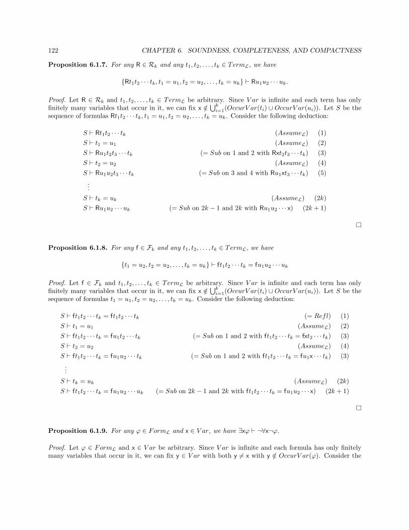
122 CHAPTER 6. SOUNDNESS, COMPLETENESS, AND COMPACTNESS
Proposition 6.1.7. For any R ∈ Rk and any t1, t2, . . . , tk ∈ TermL, we have
{Rt1t2 · · · tk, t1 = u1, t2 = u2, . . . , tk = uk} ` Ru1u2 · · ·uk.
Proof. Let R ∈ Rk and t1, t2, . . . , tk ∈ TermL be arbitrary. Since V ar is infinite and each term has onlyfinitely many variables that occur in it, we can fix x /∈
⋃ki=1(OccurV ar(ti) ∪ OccurV ar(ui)). Let S be the
sequence of formulas Rt1t2 · · · tk, t1 = u1, t2 = u2, . . . , tk = uk. Consider the following deduction:
S ` Rt1t2 · · · tk (AssumeL) (1)
S ` t1 = u1 (AssumeL) (2)
S ` Ru1t2t3 · · · tk (= Sub on 1 and 2 with Rxt2t3 · · · tk) (3)
S ` t2 = u2 (AssumeL) (4)
S ` Ru1u2t3 · · · tk (= Sub on 3 and 4 with Ru1xt3 · · · tk) (5)
...
S ` tk = uk (AssumeL) (2k)
S ` Ru1u2 · · ·uk (= Sub on 2k − 1 and 2k with Ru1u2 · · · x) (2k + 1)
Proposition 6.1.8. For any f ∈ Fk and any t1, t2, . . . , tk ∈ TermL, we have
{t1 = u2, t2 = u2, . . . , tk = uk} ` ft1t2 · · · tk = fu1u2 · · ·uk
Proof. Let f ∈ Fk and t1, t2, . . . , tk ∈ TermL be arbitrary. Since V ar is infinite and each term has onlyfinitely many variables that occur in it, we can fix x /∈
⋃ki=1(OccurV ar(ti) ∪ OccurV ar(ui)). Let S be the
sequence of formulas t1 = u1, t2 = u2, . . . , tk = uk. Consider the following deduction:
S ` ft1t2 · · · tk = ft1t2 · · · tk (= Refl) (1)
S ` t1 = u1 (AssumeL) (2)
S ` ft1t2 · · · tk = fu1t2 · · · tk (= Sub on 1 and 2 with ft1t2 · · · tk = fxt2 · · · tk) (3)
S ` t2 = u2 (AssumeL) (4)
S ` ft1t2 · · · tk = fu1u2 · · · tk (= Sub on 1 and 2 with ft1t2 · · · tk = fu1x · · · tk) (3)
...
S ` tk = uk (AssumeL) (2k)
S ` ft1t2 · · · tk = fu1u2 · · ·uk (= Sub on 2k − 1 and 2k with ft1t2 · · · tk = fu1u2 · · · x) (2k + 1)
Proposition 6.1.9. For any ϕ ∈ FormL and x ∈ V ar, we have ∃xϕ ` ¬∀x¬ϕ.
Proof. Let ϕ ∈ FormL and x ∈ V ar be arbitrary. Since V ar is infinite and each formula has only finitelymany variables that occur in it, we can fix y ∈ V ar with both y 6= x with y /∈ OccurV ar(ϕ). Consider the

6.1. SYNTACTIC IMPLICATION AND SOUNDNESS 123
following deduction:
ϕyx,¬¬∀x¬ϕ,¬∀x¬ϕ ` ¬∀x¬ϕ (AssumeL) (1)
ϕyx,¬¬∀x¬ϕ,¬∀x¬ϕ ` ¬¬∀x¬ϕ (AssumeL) (2)
ϕyx,¬¬∀x¬ϕ ` ∀x¬ϕ (Contr on 1 and 2) (3)
ϕyx,¬¬∀x¬ϕ ` ¬ϕy
x (∀E on 3) (4)
ϕyx,¬¬∀x¬ϕ ` ϕy
x (AssumeL) (5)
ϕyx ` ¬∀x¬ϕ (Contr on 4 and 5) (6)
∃xϕ ` ¬∀x¬ϕ (∃P on 6) (7)
Proposition 6.1.10. For any ϕ ∈ FormL and x ∈ V ar, we have ¬∃x¬ϕ ` ∀xϕ.
Proof. Let ϕ ∈ FormL and x ∈ V ar be arbitrary. Since V ar is infinite and each formula has only finitelymany variables that occur in it, we can fix y ∈ V ar with both y 6= x with y /∈ OccurV ar(ϕ). Consider thefollowing deduction:
¬∃x¬ϕ,¬ϕyx ` ¬∃x¬ϕ (AssumeL) (1)
¬∃x¬ϕ,¬ϕyx ` ¬ϕy
x (AssumeL) (2)
¬∃x¬ϕ,¬ϕyx ` ∃x¬ϕ (∃I on 2) (3)
¬∃x¬ϕ ` ϕyx (Contr on 1 and 3) (4)
¬∃x¬ϕ ` ∀xϕ (∀I on 4) (5)
The following definition and results following in precisely the same way as they did for propositional logic(because we still include all of the old proof rules).
Definition 6.1.11. Γ is inconsistent if there exists θ ∈ FormL such that Γ ` θ and Γ ` ¬θ. Otherwise, wesay that Γ is consistent.
Proposition 6.1.12. Let Γ1 ⊆ FormL and Γ2 ⊆ FormL be such that Γ1 ⊆ Γ2. If ϕ ∈ FormL is such thatΓ1 ` ϕ, then Γ2 ` ϕ.
Proof. See the proof of Proposition 3.4.8.
Proposition 6.1.13. Suppose that S ∈ Form∗L and ϕ ∈ FormL are such that S ` ϕ. If T is any permutationof S, then T ` ϕ.
Proof. See the proof of Proposition 3.4.9.
Proposition 6.1.14. If Γ is inconsistent, then Γ ` ϕ for all ϕ ∈ FormL.
Proof. See the proof of Proposition 3.4.10.
Proposition 6.1.15. Let Γ ⊆ FormL and let ϕ ∈ FormL.
1. If Γ ∪ {ϕ} is inconsistent, then Γ ` ¬ϕ.
2. If Γ ∪ {¬ϕ} is inconsistent, then Γ ` ϕ.
Proof. See the proof of Proposition 3.4.11.

124 CHAPTER 6. SOUNDNESS, COMPLETENESS, AND COMPACTNESS
Corollary 6.1.16. If Γ ⊆ FormL is consistent and ϕ ∈ FormL, then either Γ ∪ {ϕ} is consistent orΓ ∪ {¬ϕ} is consistent.
Proof. See the proof of Corollary 3.4.12.
Proposition 6.1.17. Let Γ ⊆ FormL and let ϕ ∈ FormL.
1. If Γ ` ϕ and Γ ∪ {ϕ} ` ψ, then Γ ` ψ.
2. If Γ ` ϕ and Γ ` ϕ→ ψ, then Γ ` ψ.
Proof. See the proof of Proposition 3.4.13.
Proposition 6.1.18. Γ ` ϕ if and only if there is a finite Γ0 ⊆ Γ such that Γ0 ` ϕ.
Proof. See the proof of Proposition 3.4.14.
Corollary 6.1.19. If every finite subset of Γ is consistent, then Γ is consistent.
Proof. See the proof of Corollary 3.4.15.
Theorem 6.1.20 (Soundness Theorem).
1. If Γ ` ϕ, then Γ � ϕ.
2. Every satisfiable set of formulas is consistent.
Proof.
1. As in the proof of the Soundness Theorem for propositional logic, we prove the following fact: IfS ∈ Form∗L and ϕ ∈ FormL are such that S ` ϕ, then S � ϕ. To see why this suffices, suppose thatΓ ` ϕ. By definition, we can then fix S ∈ Γ∗ with S ` ϕ. From here we can conclude that S � ϕ.Since every element of S is an element of Γ, it follows that Γ � ϕ.
We now prove the statement “Whenever S ` ϕ, we have S � ϕ” by induction. In other words, if G isthe set generated by starting with AssumeL ∪ EqReflL and using our proof rules, and we let
X = {(S, ϕ) ∈ G : S � ϕ},
then we show by induction on G that X = G. We begin by noting that if ϕ appears in the sequenceS, then we trivially have S � ϕ by definition. Therefore, (S, ϕ) ∈ X for all (S, ϕ) ∈ AssumeL. Also,for any S ∈ Form∗L and any t ∈ TermL, we have S � t = t because for any any model (M, s) of Swe trivially have s(t) = s(t), hence (M, s) � t = t. Therefore, (S, t = t) ∈ X for all S ∈ Form∗L andt ∈ TermL.
We now handle the inductive steps. All of the old rules go through in a similar manner as before.
• We first handle the = Sub rule. Suppose that S � ϕtx, that S � t = u, and that V alidSubsttx(ϕ) =1 = V alidSubstux (ϕ). We need to show that S � ϕux . Let (M, s) be an arbitrary model of S.Since S � ϕtx, we have that (M, s) � ϕtx. Also, since S � t = u, we have that (M, s) � t = u, andhence s(t) = s(u). Since
(M, s) � ϕtx
we can use Theorem 4.6.7 together with the fact that V alidSubsttx(ϕ) = 1 to conclude that
(M, s[x⇒ s(t)]).

6.1. SYNTACTIC IMPLICATION AND SOUNDNESS 125
Since s(t) = s(u), it follows that(M, s[x⇒ s(u)]).
Finally, we can use Theorem 4.6.7 together with the fact that V alidSubstux (ϕ) = 1 to concludethat
(M, s) � ϕux .
Since (M, s) was an arbitrary model of S, it follows that S � ϕux .
• We now handle the ∃I rule. Suppose that S � ϕtx where V alidSubsttx(ϕ) = 1. We need to showthat S � ∃xϕ. Let (M, s) be an arbitrary model of S. Since S � ϕtx, it follows that (M, s) � ϕtx.Using Theorem 4.6.7 together with the fact that V alidSubsttx(ϕ) = 1, we have
(M, s[x⇒ s(t)]).
Therefore, there exists a ∈M such that
(M, s[x⇒ a]),
from which we conclude that(M, s) � ∃xϕ.
Since (M, s) was an arbitrary model of S, it follows that S � ∃xϕ.
• Let’s next attack the ∃P rule. Suppose that S, ϕyx � ψ, that y /∈ FreeV ar(S,∃xϕ,ψ), and that
V alidSubstyx(ϕ) = 1. We need to show that S, ∃xϕ � ψ. Let (M, s) be an arbitrary model ofS, ∃xϕ. Since (M, s) � ∃xϕ, we may fix a ∈M such that (M, s[x⇒ a]) � ϕ. We first divide intotwo cases to show that (M, s[y⇒ a]) � ϕy
x.
– Case 1: Suppose that y = x. We then have ϕyx = ϕx
x = ϕ and s[x ⇒ a] = s[y ⇒ a], hence(M, s[y⇒ a]) � ϕy
x because (M, s[x⇒ a]) � ϕ.
– Case 2: Suppose that y 6= x. We know that (M, s[x ⇒ a]) � ϕ, so since y 6= x and y /∈FreeV ar(ϕ), we can conclude that
(M, (s[y⇒ a])[x⇒ a]) � ϕ.
From here, it follows that
(M, (s[y⇒ a])[x⇒ s[y⇒ a](y)]) � ϕ,
so using the Theorem 4.6.7 together with the fact that V alidSubstyx(ϕ) = 1, we conclude that
(M, s[y⇒ a]) � ϕyx.
Thus, (M, s[y⇒ a]) � ϕyx in either case. Now since (M, s) � γ for all γ ∈ S and y /∈ FreeV ar(S),
we have (M, s[y⇒ a]) � γ for all γ ∈ S. Since we are assuming that S, ϕyx � ψ, and we know that
(M, s[y⇒ a]) � γ for all γ ∈ S, and that (M, s[y⇒ a]) � ϕyx, we conclude that (M, s[y⇒ a]) � ψ.
Finally, since y /∈ FreeV ar(ψ), it follows that (M, s) � ψ.
• We next do the ∀E rule. Suppose that S � ∀xϕ and that t ∈ TermL is such that V alidSubsttx(ϕ) =1. We need to show that S � ϕtx. Let (M, s) be an arbitrary model of S. Since S � ∀xϕ, it followsthat that (M, s) � ∀xϕ. By definition, we conclude that (M, s[x ⇒ a]) � ϕ for all a ∈ M . Nows(t) ∈M , so in particular we have that
(M, s[x⇒ s(t)]) � ϕ
Using Theorem 4.6.7) together with the fact that V alidSubsttx(ϕ) = 1, it follows that
(M, s) � ϕtx.

126 CHAPTER 6. SOUNDNESS, COMPLETENESS, AND COMPACTNESS
• We finally end with the ∀I rule. Suppose that S � ϕyx, that y /∈ FreeV ar(S, ∀xϕ), and that
V alidSubstyx(ϕ) = 1. We need to show that S � ∀xϕ. Let (M, s) be an arbitrary model of S. Wehandle two cases.
– Case 1: Suppose that y = x. Since y = x, we have ϕyx = ϕx
x = ϕ. Let a ∈M be arbitrary. Since(M, s) is a model of S, we know that (M, s) � γ for all γ ∈ S. Now we are assuming thatx = y /∈ FreeV ar(S), so we may conclude that (M, s[x⇒ a]) � γ for all γ ∈ S. Since we arealso assuming that S � ϕy
x, it follows that (M, s[x ⇒ a]) � ϕyx, and hence (M, s[x ⇒ a]) � ϕ
(because ϕyx = ϕ in this case). Now a ∈ M was arbitrary, so (M, s[x ⇒ a]) � ϕ for every
a ∈M . Therefore, by definition, we have (M, s) � ∀xϕ.
– Case 2: Suppose that y 6= x. Let a ∈M be arbitrary. Since (M, s) is a model of S, we knowthat (M, s) � γ for all γ ∈ S. Now we are assuming that y /∈ FreeV ar(S), so we may concludethat (M, s[y ⇒ a]) � γ for all γ ∈ S. Since we are also assuming that S � ϕy
x, it follows that(M, s[y ⇒ a]) � ϕy
x. Using Theorem 4.6.7 together with the fact V alidSubstyx(ϕ) = 1, wehave
(M, (s[y⇒ a])[x⇒ s[y⇒ a](y)]) � ϕ,
and hence(M, (s[y⇒ a])[x⇒ a]) � ϕ.
Since we are assuming that y /∈ FreeV ar(ϕ) and y 6= x, it follows that
(M, s[x⇒ a]) � ϕ.
Now a ∈M was arbitrary, so (M, s[x⇒ a]) � ϕ for every a ∈M , hence (M, s) � ∀xϕ.
The result follows by induction.
2. Let Γ be an arbitrary satisfiable set of formulas. Fix a model (M, s) of Γ. Suppose that Γ is inconsistent,and fix θ ∈ FormL such that Γ ` θ and Γ ` ¬θ. We then have Γ � θ and Γ � ¬θ by part (1), hence(M, s) � θ and (M, s) � ¬θ, a contradiction. It follows that Γ is consistent.
6.2 Completeness
Let’s recall the outline of our proof of the Completeness Theorem for propositional logic. We wanted toshow that every consistent set was satisfiable. Suppose then that we had an arbitrary consistent set Γ. SinceΓ could consist of many very complex formulas, and perhaps no simple formulas, it seemed hard to definean appropriate truth assignment. Thus, our first step was to enlarge Γ to a consistent and complete set ∆.In particular, we then had that property that for every A ∈ P , either A ∈ ∆ or ¬A ∈ ∆. With this start,we were able to define an appropriate truth assignment M , and then continue to use the fact that ∆ wascomplete to verify that vM (δ) = 1 for all δ ∈ ∆.
Suppose now that we are in the first-order logic setting. Thus, we have a language L and a set Γ ⊆ FormLthat is consistent. We will take our cue from propositional logic, and first expand the set appropriately. Hereis the definition.
Definition 6.2.1. Suppose that L is a language and that ∆ ⊆ FormL. We say that ∆ is complete if for allϕ ∈ FormL, either ϕ ∈ ∆ or ¬ϕ ∈ ∆.
Notice that this definition resembles the definition of a complete theory, but differs in the fact thatwe are assuming that either ϕ ∈ ∆ or ¬ϕ ∈ ∆ for each formula ϕ (which is more general than for eachsentence). Let’s assume that we can indeed expand every consistent set Γ to a set ∆ that is both consistent

6.2. COMPLETENESS 127
and complete (the proof is completely analogous to the proof in the propositional logic case). In order toshow that Γ is satisfiable, it suffices to show that ∆ is satisfiable. Thus, we need to construct an L-structureM and a variable assignment s : V ar → M such that (M, s) � δ for all δ ∈ ∆. Now all that we have is thesyntactic information that ∆ provides, so it seems that the only way to proceed is to define our M fromthese syntactic objects. Since terms intuitively name elements, it is natural to try to define the universe Mto simply be TermL. We would then define the structure as follows:
1. cM = c for all c ∈ C.
2. RM = {(t1, t2, . . . , tk) ∈Mk : Rt1t2 . . . tk ∈ ∆} for all R ∈ Rk.
3. fM(t1, t2, . . . , tk) = ft1t2 · · · tk for all f ∈ Fk and all t1, t2, . . . , tk ∈M .
Finally, it seems reasonable to define s : V ar →M to be the variable assignment s(x) = x for all x ∈ V ar.Despite the promise and elegance of this approach, there is one minor problem and one major problem
that we must address. First, let’s think about the minor problem. Suppose that L = {f, e} is the basic grouptheory language, and that Γ is the set of group axioms. Suppose that ∆ ⊇ Γ is consistent and complete.We then have fee = e ∈ ∆ because Γ ` fee = e. However, the two terms fee and e are syntactically differentobjects. In other words, if we allow the above idea by letting M = TermL, we would run into a problembecause fee and e are distinct, despite the fact that ∆ says that they must be equal. Of course, when wehave distinct objects that we want to make equal, we should define an equivalence relation. The naturalrelation here is to define ∼ on TermL by letting t ∼ u mean that t = u ∈ ∆. We would then need to checkthat ∼ is an equivalence relation and that the definition of the structure above is independent of our choiceof representatives for the classes. This is all fairly straightforward, and we will carry the details below.
On to the more serious obstacle. Suppose that L = {P} where P is a unary relation symbol. LetΓ = {¬Px : x ∈ V ar} ∪ {¬(x = y) : x, y ∈ V ar with x 6= y} ∪ {∃xPx} and notice that Γ is consistent becauseit is satisfiable (let M = N, let s : V ar → N be s(xk) = k + 1, and let PM = {0}). Suppose that ∆ ⊇ Γ isconsistent and complete. In the structureM described above, we have M = TermL = V ar (notice that theequivalence relation defined above will be trivial in this case). Thus, since (M, s) � ¬Px for all x ∈ V ar, itfollows that (M, s) 6� ∃xPx. Hence, M is not a model of ∆.
The problem in the above example is that there was an existential statement in ∆, but whenever weplugged a term in for the quantified variable, the resulting formula was not in ∆. Since we are building ourstructure directly from the terms, this is a serious problem. However, if ∆ had the following property, thenthis problem would not arise.
Definition 6.2.2. Let L be a language and let Γ ⊆ FormL. We say that Γ contains witnesses if for allϕ ∈ FormL and all x ∈ V ar, there exists c ∈ C such that (∃xϕ)→ ϕc
x ∈ Γ.
Our goal then is to show that if Γ is consistent, then there exists a ∆ ⊇ Γ which is consistent, complete,and contains witnesses. On the face of it, this is not true, as the above example shows (because there are noconstant symbols). However, if we allow ourselves to expand our language with new constant symbols, wecan repeatedly add witnessing statements by using these fresh constant symbols as our witnesses. The keyquestion we need to consider is the following. Suppose that L is a language and Γ ⊆ FormL is consistent.If we expand the language L to a language L′ obtained by adding a new constant symbol, is the set Γ stillconsistent when viewed as a set of L′ formulas? It might seem absolutely harmless to add a new constantsymbol about which we say nothing (and it’s not hard very hard to see that it is semantically harmless),but we are introducing new deductions in L’. We need a way to convert a possibly bad L′-deduction into asimilarly bad L-deduction to argue that Γ is still consistent as a set of L′-formulas.
We can also define substitution of variables for constants in the obvious recursive fashion.
Definition 6.2.3. Let z ∈ V ar and let c ∈ TermC. We define a function Substzc : TermL → TermL, wherewe use tzc to denote Substzc(t), as follows:
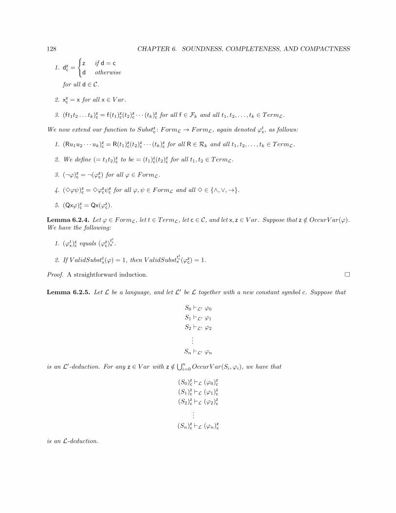
128 CHAPTER 6. SOUNDNESS, COMPLETENESS, AND COMPACTNESS
1. dzc =
{z if d = c
d otherwise
for all d ∈ C.
2. xzc = x for all x ∈ V ar.
3. (ft1t2 . . . tk)zc = f(t1)zc(t2)zc · · · (tk)zc for all f ∈ Fk and all t1, t2, . . . , tk ∈ TermL.
We now extend our function to Substzc : FormL → FormL, again denoted ϕtx, as follows:
1. (Ru1u2 · · ·uk)zc = R(t1)zc(t2)zc · · · (tk)zc for all R ∈ Rk and all t1, t2, . . . , tk ∈ TermL.
2. We define (= t1t2)zc to be = (t1)zc(t2)zc for all t1, t2 ∈ TermL.
3. (¬ϕ)zc = ¬(ϕzc) for all ϕ ∈ FormL.
4. (3ϕψ)zc = 3ϕzcψ
zc for all ϕ,ψ ∈ FormL and all 3 ∈ {∧,∨,→}.
5. (Qxϕ)zc = Qx(ϕzc).
Lemma 6.2.4. Let ϕ ∈ FormL, let t ∈ TermL, let c ∈ C, and let x, z ∈ V ar. Suppose that z /∈ OccurV ar(ϕ).We have the following:
1. (ϕtx)zc equals (ϕz
c)tzcx .
2. If V alidSubsttx(ϕ) = 1, then V alidSubsttzcx (ϕz
c) = 1.
Proof. A straightforward induction.
Lemma 6.2.5. Let L be a language, and let L′ be L together with a new constant symbol c. Suppose that
S0 `L′ ϕ0
S1 `L′ ϕ1
S2 `L′ ϕ2
...
Sn `L′ ϕn
is an L′-deduction. For any z ∈ V ar with z /∈⋃ni=0OccurV ar(Si, ϕi), we have that
(S0)zc `L (ϕ0)zc
(S1)zc `L (ϕ1)zc
(S2)zc `L (ϕ2)zc...
(Sn)zc `L (ϕn)zc
is an L-deduction.

6.2. COMPLETENESS 129
Proof. We prove by induction on i that
(S0)zc `L (ϕ0)zc
(S1)zc `L (ϕ1)zc
(S2)zc `L (ϕ2)zc...
(Si)zc `L (ϕi)
zc
is an L-deduction.If ϕ ∈ S, then ϕz
c ∈ Szc .
Suppose that line i is S ` t = t where t ∈ TermL′ . Since (t = t)zc equals tzc = tzc, we can place Szc ` tzc = tzc
on line i by the = Refl rule.Suppose that S `L′ ϕ∧ψ was a previous line and we inferred S `L′ ϕ. Inductively, we have Sz
c `L (ϕ ∧ ψ)zcon the corresponding line. Since (ϕ ∧ ψ)zc = ϕz
c ∧ ψzc, we may use the ∧EL rule to put Sz
c `L ϕzc on the
corresponding line. The other propositional rules are similarly uninteresting.Suppose that S `L′ ϕtx and S `L′ t = u were previous lines, that V alidSubsttx(ϕ) = 1 = V alidSubstux (ϕ),
and we inferred S `L′ ϕux . Inductively, we have Szc `L (ϕtx)
zc and Sz
c `L (t = u)zc on the corresponding lines.
Now (ϕtx)zc equals (ϕz
c)tzcx by the previous lemma, and (t = u)zc equals tzc = uzc. Thus, we have Sz
c `L (ϕzc)tzcx
and Szc `L tzc = uzc on the corresponding lines. Using the fact that V alidSubsttx(ϕ) = 1 = V alidSubstux (ϕ),
we can use the previous lemma to conclude that that V alidSubsttzcx (ϕz
c) = 1 = V alidSubstuzc
x (ϕzc). Hence, we
may use that = Sub rule to put Szc `L (ϕz
c)uzc
x on the corresponding line. We now need only note that (ϕzc)uzc
x
equals (ϕux )zc by the previous lemma.Suppose that S `L′ ϕtx where V alidSubsttx(ϕ) = 1 was a previous line and we inferred S `L′ ∃xϕ.
Inductively, we have Szc `L (ϕtx)
zc on the corresponding line. Now (ϕtx)
zc equals (ϕz
c)tzcx and V alidSubst
tzcx (ϕz
c) = 1by the previous lemma. Hence, we may use the ∃I rule to put Sz
c `L ∃x(ϕzc) on the corresponding line. We
now need only note that ∃x(ϕzc) equals (∃xϕ)zc.
The other rules are similar.
Corollary 6.2.6. Let L be a language, let Γ ⊆ FormL, and let ϕ ∈ FormL.
1. Let L′ be L together with a new constant symbol. If Γ `L′ ϕ, then Γ `L ϕ.
2. Let L′ be L together with finitely many new constant symbols. If Γ `L′ ϕ, then Γ `L ϕ.
3. Let L′ be L together with (perhaps infinitely many) new constant symbols. If Γ `L′ ϕ, then Γ `L ϕ.
Proof.
1. Since Γ `L′ ϕ, we may fix an L′-deduction
S0 `L′ ϕ0
S1 `L′ ϕ1
S2 `L′ ϕ2
...
Sn `L′ ϕn
such that each Si ⊆ Form∗L′ , and where Sn ∈ Γ∗ and ϕn = ϕ. Fix y ∈ V ar such that
y /∈n⋃i=0
OccurV ar(Si, ϕi).

130 CHAPTER 6. SOUNDNESS, COMPLETENESS, AND COMPACTNESS
From Lemma 6.2.5, we have that
(S0)yc `L (ϕ0)yc
(S1)yc `L (ϕ1)yc
(S2)yc `L (ϕ2)yc...
(Sn)yc `L (ϕn)yc
is an L-deduction. Since Sn ∈ Γ∗ ⊆ Form∗L and ϕ ∈ FormL, it follows that (Sn)yc = Sn and (ϕn)yc = ϕ.Thus, Sn `L ϕ and so Γ `L ϕ.
2. This is proved by induction on the number of new constant symbols, using part (1) for both the basecase and the inductive step.
3. Since Γ `L′ ϕ, we may fix an L′-deduction
S0 `L′ ϕ0
S1 `L′ ϕ1
S2 `L′ ϕ2
...
Sn `L′ ϕn
such that each Si ⊆ Form∗L′ , and where Sn ∈ Γ∗ and ϕn = ϕ. Let {c0, c1, . . . , cm} be all of theconstant symbols appearing in some Si or ϕi, and let L0 = L ∪ {c0, c1, . . . , cm}. We then have that
S0 `L0 ϕ0
S1 `L0 ϕ1
S2 `L0 ϕ2
...
Sn `L0 ϕn
is an L0-deduction, so Γ `L0 ϕ. Therefore, Γ `L ϕ by part (2).
Corollary 6.2.7. Let L be a language and let L′ be L together with (perhaps infinitely many) new constantsymbols. Let Γ ⊆ FormL. Γ is L-consistent if and only if Γ is L′-consistent.
Proof. Since any L-deduction is also a L′-deduction, if Γ is L-inconsistent then it is trivially L′-inconsistent.Suppose that Γ is L′-inconsistent. We then have that Γ `L′ ϕ for all ϕ ∈ FormL by Proposition 6.1.14,hence Γ `L ϕ for all ϕ ∈ FormL by Corollary 6.2.6. Therefore, Γ is L-inconsistent.
Corollary 6.2.8 (Generalization on Constants). Let L be a language, and let L′ be L together with a newconstant symbol c. Suppose that Γ ⊆ FormL and ϕ ∈ FormL. If Γ `L′ ϕc
x, then Γ `L ∀xϕ.

6.2. COMPLETENESS 131
Proof. Since Γ `L′ ϕcx, we may fix an L′-deduction
S0 `L′ ϕ0
S1 `L′ ϕ1
S2 `L′ ϕ2
...
Sn `L′ ϕn
such that each Si ⊆ Form∗L′ , and that Sn ∈ Γ∗ and ϕn = ϕcx. Fix y ∈ V ar such that
y /∈n⋃i=0
OccurV ar(Si, ϕi).
From Lemma 6.2.5, we have that
(S0)yc `L (ϕ0)yc
(S1)yc `L (ϕ1)yc
(S2)yc `L (ϕ2)yc...
(Sn)yc `L (ϕn)yc
is an L-deduction. Since Sn ∈ Γ∗ ⊆ Form∗L, we have (Sn)yc = Sn. Now (ϕn)yc = (ϕcx)
yc = ϕy
x. We thereforehave Sn `L ϕy
x. We may then use the ∀I rule to conclude that Sn `L ∀xϕ. Since Sn ∈ Γ∗, it follows thatΓ `L ∀xϕ.
Lemma 6.2.9. For all ϕ,ψ ∈ FormL, we have ¬(ϕ→ ψ) ` ϕ ∧ ¬ψ.
Proof. Let ϕ,ψ ∈ FormL be arbitrary. Consider the following deduction:
¬(ϕ→ ψ),¬ϕ,ϕ,¬ψ ` ϕ (AssumeL) (1)
¬(ϕ→ ψ),¬ϕ,ϕ,¬ψ ` ¬ϕ (AssumeL) (2)
¬(ϕ→ ψ),¬ϕ,ϕ ` ψ (Contr on 1 and 2) (3)
¬(ϕ→ ψ),¬ϕ ` ϕ→ ψ (→ I on 3) (4)
¬(ϕ→ ψ),¬ϕ ` ¬(ϕ→ ψ) (AssumeL) (5)
¬(ϕ→ ψ) ` ϕ (Contr on 4 and 5) (6)
¬(ϕ→ ψ),¬¬ψ,ϕ,¬ψ ` ¬ψ (AssumeL) (7)
¬(ϕ→ ψ),¬¬ψ,ϕ,¬ψ ` ¬¬ψ (AssumeL) (8)
¬(ϕ→ ψ),¬¬ψ,ϕ ` ψ (Contr on 7 and 8) (9)
¬(ϕ→ ψ),¬¬ψ ` ϕ→ ψ (→ I on 9) (10)
¬(ϕ→ ψ),¬¬ψ ` ¬(ϕ→ ψ) (AssumeL) (11)
¬(ϕ→ ψ) ` ¬ψ (Contr on 10 and 11) (12)
¬(ϕ→ ψ) ` ϕ ∧ ¬ψ (∧I on 6 and 12) (13)
Lemma 6.2.10. Let L be a language, and let L′ be L together with a new constant symbol c. Let Γ ⊆ FormLand let ϕ ∈ FormL. If Γ is L-consistent, then Γ ∪ {(∃xϕ)→ ϕc
x} is L′-consistent.

132 CHAPTER 6. SOUNDNESS, COMPLETENESS, AND COMPACTNESS
Proof. We prove the contrapositive. Suppose then that Γ∪{(∃xϕ)→ ϕcx} is L′-inconsistent. By Proposition
6.1.15, we then have thatΓ `L′ ¬((∃xϕ)→ ϕc
x).
From Lemma 6.2.9, we have¬((∃xϕ)→ ϕcx) `L′ (∃xϕ) ∧ ¬(ϕcx),
and henceΓ ∪ {¬((∃xϕ)→ ϕcx)} `L′ (∃xϕ) ∧ ¬(ϕcx).
Using Proposition 6.1.17, we conclude that
Γ `L′ (∃xϕ) ∧ ¬(ϕcx).
Using the ∧EL rule, we conclude that Γ `L′ ∃xϕ. Since ∃xϕ `L′ ¬∀x¬ϕ by Proposition 6.1.9, we can againuse Proposition 6.1.17 to conclude that Γ `L′ ¬∀x¬ϕ. Since Γ ⊆ FormL and ¬∀x¬ϕ ∈ FormL, Corollary6.2.6 allows us to conclude that
Γ `L ¬∀x¬ϕ.Using the ∧ER rule instead, together with the fact that ¬(ϕc
x) equals (¬ϕ)cx, we also have Γ `L′ (¬ϕ)cx, so
Γ `L ∀x¬ϕ
by Generalization on Constants. Therefore, Γ is L-inconsistent.
Lemma 6.2.11. Let L be a language and let Γ ⊆ FormL be L-consistent. There exists a language L′ ⊇ L,obtained from L by only adding constant symbols, and Γ′ ⊆ FormL′ with the following properties:
1. Γ ⊆ Γ′.
2. Γ′ is L′-consistent.
3. For all ϕ ∈ FormL and all x ∈ V ar, there exists c ∈ C such that (∃xϕ)→ ϕcx ∈ Γ′.
Proof. For each ϕ ∈ FormL and each x ∈ V ar, let cϕ,x be a new constant symbol (distinct from all symbolsin L). Let L′ = L ∪ {cϕ,x : ϕ ∈ FormL and x ∈ V ar}. Let
Γ′ = Γ ∪ {(∃xϕ)→ ϕcϕ,xx : ϕ ∈ FormL and x ∈ V ar}.
Conditions 1 and 3 are clear, so we need only check that Γ′ is L′-consistent. By Corollary 6.1.19, it sufficesto check that all finite subsets of Γ′ are L′-consistent, and for this it suffices to show that
Γ ∪ {(∃x1ϕ1)→ (ϕ1)cϕ1,x1x1 , (∃x2ϕ2)→ (ϕ2)
cϕ2,x2x2 , . . . , (∃xnϕn)→ (ϕn)
cϕn,xnxn }
is L′-consistent whenever ϕ1, ϕ2, . . . , ϕn ∈ FormL and x1, x2, . . . , xn ∈ V ar. Formally, one can prove this byinduction on n. A slightly informal argument is as as follows. Let ϕ1, ϕ2, . . . , ϕn ∈ FormL and x1, x2, . . . , xn ∈V ar be arbitrary. Since Γ is L-consistent, we can apply Lemma 6.2.10 to conclude that
Γ ∪ {(∃x1ϕ1)→ (ϕ1)cϕ1,x1x1 }
is (L ∪ {cϕ1,x1})-consistent. Applying Lemma 6.2.10, we conclude that
Γ ∪ {(∃x1ϕ1)→ (ϕ1)cϕ1,x1x1 , (∃x2ϕ2)→ (ϕ2)
cϕ2,x2x2 }
is (L ∪ {cϕ1,x1 , cϕ2,x2}). By repeated applications of Lemma 6.2.10, we eventually conclude that
Γ ∪ {(∃x1ϕ1)→ (ϕ1)cϕ1,x1x1 , (∃x2ϕ2)→ (ϕ2)
cϕ2,x2x2 , . . . , (∃xnϕn)→ (ϕn)
cϕn,xnxn }
is (L ∪ {cϕ1,x1 , cϕ2,x2 , . . . , cϕn,xn})-consistent. Therefore,
Γ ∪ {(∃x1ϕ1)→ (ϕ1)cϕ1,x1x1 , (∃x2ϕ2)→ (ϕ2)
cϕ2,x2x2 , . . . , (∃xnϕn)→ (ϕn)
cϕn,xnxn }
is L′-consistent by Corollary 6.2.7, which completes the proof by the above comments.

6.2. COMPLETENESS 133
Proposition 6.2.12. Let L be a language and let Γ ⊆ FormL be consistent. There exists a language L′ ⊇ L,obtained from L by only adding constant symbols, and Γ′ ⊆ FormL′ with the following properties:
1. Γ ⊆ Γ′.
2. Γ′ is L′-consistent.
3. Γ′ contains witnesses.
Proof. Let L0 = L and Γ0 = Γ. For each n ∈ N, use Lemma 6.2.11 to obtain Ln+1 and Γn+1 from Ln andΓn. Now let L′ =
⋃n∈N L and set Γ′ =
⋃n∈N Γn. We then clearly have properties (1) and (3), and property
(2) follows from Corollary 6.1.19 and Corollary 6.2.7.
Proposition 6.2.13. If Γ is consistent, then there exists a set ∆ ⊇ Γ which is consistent and complete.
Proof. Exactly the same proof as the propositional logic case, using Zorn’s Lemma in the uncountable case(see Proposition 3.5.4 and Proposition 3.5.7).
Proposition 6.2.14. Let L be a language. If Γ ⊆ L is consistent, then there a language L′ ⊇ L, obtainedfrom L by only adding constant symbols, and ∆ ⊆ FormL′ with the following properties:
• Γ ⊆ ∆.
• ∆ is consistent.
• ∆ is complete.
• ∆ contains witnesses.
Proof. First apply Proposition 6.2.12 to obtain L′ and Γ′, and then apply Proposition 6.2.13 to obtain ∆from Γ′
Lemma 6.2.15. Suppose that ∆ is consistent and complete. If ∆ ` ϕ, then ϕ ∈ ∆.
Proof. Suppose that ∆ ` ϕ. Since ∆ is complete, we have that either ϕ ∈ ∆ or ¬ϕ ∈ ∆. Now if ¬ϕ ∈ ∆,then we would would trivially have ∆ ` ¬ϕ (in addition to our assumed ∆ ` ϕ), contradicting the fact that∆ is consistent. It follows that ϕ ∈ ∆.
Lemma 6.2.16. Suppose that ∆ is consistent, complete, and contains witnesses. For every t ∈ TermL,there exists c ∈ C such that t = c ∈ ∆.
Proof. Let t ∈ TermL. Fix x ∈ V ar such that x /∈ OccurV ar(t). Since ∆ contains witnesses, we may fixc ∈ C such that (∃x(t = x))→ (t = c) ∈ ∆ (using the formula t = x). Now ∆ ` (t = x)tx, so we may use the∃I rule (because V alidSubsttx(t = x) = 1) to conclude that ∆ ` ∃x(t = x). Since we have both ∆ ` ∃x(t = x)and ∆ ` (∃x(t = x)) → (t = c), we can apply Proposition 6.1.17 to conclude that ∆ ` t = c. Using Lemma6.2.15, it follows that that t = c ∈ ∆.
Lemma 6.2.17. Suppose that ∆ is consistent, complete, and contains witnesses. We have
1. ¬ϕ ∈ ∆ if and only if ϕ /∈ ∆.
2. ϕ ∧ ψ ∈ ∆ if and only if ϕ ∈ ∆ and ψ ∈ ∆.
3. ϕ ∨ ψ ∈ ∆ if and only if ϕ ∈ ∆ or ψ ∈ ∆.
4. ϕ→ ψ ∈ ∆ if and only if ϕ /∈ ∆ or ψ ∈ ∆.

134 CHAPTER 6. SOUNDNESS, COMPLETENESS, AND COMPACTNESS
5. ∃xϕ ∈ ∆ if and only if there exists c ∈ C such that ϕcx ∈ ∆.
6. ∀xϕ ∈ ∆ if and only if ϕcx ∈ ∆ for all c ∈ C.
Proof. The proofs of the first four statements are identical to the proofs in the propositional logic case (seeLemma 3.5.9). We prove the last two.
5. Suppose first that ∃xϕ ∈ ∆. Since ∆ contains witnesses, we may fix c ∈ C such that (∃xϕ)→ ϕcx ∈ ∆.
We therefore have ∆ ` ∃xϕ and ∆ ` (∃xϕ)→ ϕcx, hence ∆ ` ϕc
x by Proposition 6.1.17. Using Lemma6.2.15, we conclude that ϕc
x ∈ ∆.
Conversely, suppose that there exists c ∈ C such that ϕcx ∈ ∆. We then have ∆ ` ϕc
x, hence ∆ ` ∃xϕusing the ∃I rule (notice that V alidSubstcx(ϕ) = 1). Using Lemma 6.2.15, we conclude that ∃xϕ ∈ ∆.
6. Suppose first that ∀xϕ ∈ ∆. We then have ∆ ` ∀xϕ, hence ∆ ` ϕcx for all c ∈ C using the ∀E rule
(notice that V alidSubstcx(ϕ) = 1 for all c ∈ C). Using Lemma 6.2.15, we conclude that ϕcx ∈ ∆ for all
c ∈ C.Conversely, suppose that ϕc
x ∈ ∆ for all c ∈ C. Since ∆ is consistent, this implies that there does notexist c ∈ C with ¬(ϕc
x) = (¬ϕ)cx ∈ ∆. Therefore, ∃x¬ϕ /∈ ∆ by part 5, so ¬∃x¬ϕ ∈ ∆ by part (1). Itfollows from Proposition 6.1.10 that ∆ ` ∀xϕ. Using Lemma 6.2.15, we conclude that ∀xϕ ∈ ∆.
Proposition 6.2.18. If ∆ is consistent, complete, and contains witnesses, then ∆ is satisfiable.
Proof. Suppose that ∆ is consistent, complete, and contains witnesses. Define a relation ∼ on TermL byletting t ∼ u if t = u ∈ ∆. We first check that ∼ is an equivalence relation. Reflexivity follows from the= Refl rule and Lemma 6.2.15. Symmetry and transitivity follow from Proposition 6.1.5 and Proposition6.1.6, together with Lemma 6.2.15.
We now define our L-structure M. We first let M = TermL/ ∼ be the set of all equivalence classesof our equivalence relation. For each t ∈ TermL, we let [t] denote the equivalence class of t. Notice thatM = {[c] : c ∈ C} by Lemma 6.2.16. We now finish our description of the L-structure M by saying how tointerpret the constant, relation, and function symbols. We define the following:
1. cM = [c] for all c ∈ C.
2. RM = {([t1], [t2], . . . , [tk]) ∈Mk : Rt1t2 · · · tk ∈ ∆} for all R ∈ Rk.
3. fM([t1], [t2], . . . , [tk]) = [ft1t2 · · · tk] for all f ∈ Fk.
Notice that our definitions of RM do not depend on our choice of representatives for the equivalence classesby Proposition 6.1.7. Similarly, our definitions of fM do not depend on our choice of representatives for theequivalences classes by Proposition 6.1.8. Finally, define s : V ar →M by letting s(x) = [x] for all x ∈ V ar.
We first show that s(t) = [t] for all t ∈ TermL by induction. We have s(c) = cM = [c] for all c ∈ C ands(x) = s(x) = [x] for all x ∈ V ar. Suppose that f ∈ Fk and t1, t2, . . . , tk ∈ TermL are such that s(ti) = [ti]for all i. We then have
s(ft1t2 · · · tk) = fM(s(t1), s(t2), . . . , s(tk))
= fM([t1], [t2], . . . , [tk]) (by induction)
= [ft1t2 · · · tk]
Therefore, s(t) = [t] for all t ∈ TermL.

6.2. COMPLETENESS 135
We now show that by induction that for all ϕ ∈ FormL, we have ϕ ∈ ∆ if and only if (M, s) � ϕ. Wefirst prove the result for ϕ ∈ AtomicFormL. Given arbitary R ∈ Rk and t1, t2, . . . , tk ∈ TermL, we have
Rt1t2 · · · tk ∈ ∆⇔ ([t1], [t2], . . . , [tk]) ∈ RM
⇔ (s(t1), s(t2), . . . , s(tk)) ∈ RM
⇔ (M, s) � Rt1t2 · · · tk.
Given arbirary t1, t2 ∈ TermL, we have
t1 = t2 ∈ ∆⇔ [t1] = [t2]
⇔ s(t1) = s(t2)
⇔ (M, s) � t1 = t2.
If the statement is true for ϕ, then
¬ϕ ∈ ∆⇔ ϕ /∈ ∆ (by Lemma 6.2.17)
⇔ (M, s) 6� ϕ (by induction)
⇔ (M, s) � ϕ.
Similarly, if the statement is true for ϕ and ψ, then
ϕ ∧ ψ ∈ ∆⇔ ϕ ∈ ∆ and ψ ∈ ∆ (by Lemma 6.2.17)
⇔ (M, s) � ϕ and (M, s) � ψ (by induction)
⇔ (M, s) � ϕ ∧ ψ
and
ϕ ∨ ψ ∈ ∆⇔ ϕ ∈ ∆ or ψ ∈ ∆ (by Lemma 6.2.17)
⇔ (M, s) � ϕ or (M, s) � ψ (by induction)
⇔ (M, s) � ϕ ∨ ψ
and finally
ϕ→ ψ ∈ ∆⇔ ϕ /∈ ∆ or ψ ∈ ∆ (by Lemma 6.2.17)
⇔ (M, s) 6� ϕ or (M, s) � ψ (by induction)
⇔ (M, s) � ϕ→ ψ.
If the statement is true for ϕ and x ∈ V ar is arbitrary, then
∃xϕ ∈ ∆⇔ There exists c ∈ C such that ϕcx ∈ ∆ (by Lemma 6.2.17)
⇔ There exists c ∈ C such that (M, s) � ϕcx (by induction)
⇔ There exists c ∈ C such that (M, s[x⇒ s(c)]) � ϕ (by the Substitution Theorem)
⇔ There exists c ∈ C such that (M, s[x⇒ [c]]) � ϕ
⇔ There exists a ∈M such that (M, s[x⇒ a]) � ϕ (since M = {[c] : c ∈ C})⇔ (M, s) � ∃xϕ

136 CHAPTER 6. SOUNDNESS, COMPLETENESS, AND COMPACTNESS
and also
∀xϕ ∈ ∆⇔ For all c ∈ C, we have ϕcx ∈ ∆ (by Lemma 6.2.17)
⇔ For all c ∈ C, we have (M, s) � ϕcx (by induction)
⇔ For all c ∈ C, we have (M, s[x⇒ s(c)]) � ϕ (by the Substitution Theorem)
⇔ For all c ∈ C, we have (M, s[x⇒ [c]])
⇔ For all a ∈M, we have (M, s[x⇒ a]) � ϕ (since M = {[c] : c ∈ C})⇔ (M, s) � ∀xϕ.
Therefore, by induction, we have ϕ ∈ ∆ if and only if (M, s) � ϕ. In particular, we have (M, s) � ϕ for allϕ ∈ ∆, hence ∆ is satisfiable.
Theorem 6.2.19 (Completeness Theorem). Let L be a language.
1. Every consistent set of formulas is satisfiable.
2. If Γ � ϕ, then Γ ` ϕ.
Proof.
1. Suppose that Γ is consistent. By Proposition 6.2.14, we may fix a language L′ ⊇ L and ∆ ⊆ FormL′
such that ∆ ⊇ Γ is consistent, complete, and contains witnesses. Now ∆ is satisfiable by Proposition6.2.18, so we may fix an L′-structure M′ together with s : V ar → M ′ such that (M′, s) � ϕ for allϕ ∈ ∆. We then have (M′, s) � γ for all γ ∈ Γ. LettingM be the restiction ofM′ to L, we then have(M, s) � γ for all γ ∈ Γ. Therefore, Γ is satisfiable.
2. Suppose that Γ � ϕ. We then have that Γ ∪ {¬ϕ} is unsatisfiable, hence Γ ∪ {¬ϕ} is inconsistent bypart 1. It follows from Proposition 6.1.15 that Γ ` ϕ.
We now give another proof of the Countable Lowenheim-Skolem Theorem which does not go through theconcept of elementary substructures.
Corollary 6.2.20 (Countable Lowenheim-Skolem Theorem). Suppose that L is countable and Γ ⊆ FormLis consistent. There exists a countable model of Γ.
Proof. Notice that if L is consistent, then the L′ formed in Lemma 6.2.11 is countable because FormL×V aris countable. Thus, each Ln in the proof of Proposition 6.2.12 is countable, so the L′ formed in Proposition6.2.12 is countable. It follows that TermL′ is countable, and since the L′-structure M we construct in theproof of Proposition 6.2.18 is formed by taking the quotient from an equivalence relation on the countableTermL′ , we can conclude that M is countable. Therefore, the L-structure which is the restriction of M toL from the proof of the Completeness Theorem is countable.
6.3 Compactness and Applications
Now that we have completed proofs of the Soundness and Completeness Theorems, we immediately obtainthe following result, which is one of the primary tools in logic.
Corollary 6.3.1 (Compactness Theorem). Let L be a language.
1. If Γ � ϕ, then there exists a finite Γ0 ⊆ Γ such that Γ0 � ϕ.

6.3. COMPACTNESS AND APPLICATIONS 137
2. If every finite subset of Γ is satisfiable, then Γ is satisfiable.
Proof.
1. Suppose that Γ � ϕ. By the Completeness Theorem, we have Γ ` ϕ. Using Proposition 6.1.18, we mayfix a finite Γ0 ⊆ Γ such that Γ0 ` ϕ. By the Soundness Theorem, we have Γ0 � ϕ.
2. If every finite subset of Γ is satisfiable, then every finite subset of Γ is consistent by the SoundnessTheorem, hence Γ is consistent by Corollary 6.1.19, and so Γ is satisfiable by the Soundness Theorem.
For our first application of Compactness, we prove another result expressing the fact that first-order logicis not powerful enough to distinguish certain aspects of cardinality. We already have the Lowenheim-SkolemTheorem saying that any satisfiable set has a countable model (assuming that L is countable), and hencefirst-order logic does not have the expressive power to force all models to be uncountable. In this case, ourdistinction is between large finite numbers and the infinite.
Proposition 6.3.2. Let L be a language. Suppose that Γ ⊆ FormL is such that for all n ∈ N, there existsa model (M, s) of Γ such that |M | > n. We then have that there exists a model (M, s) of Γ such that M isinfinite.
We give two proofs.
Proof 1. For each n ∈ N with n ≥ 2, let σn be the sentence
∃x1∃x2 . . . ∃xn
∧1≤i<j≤n
¬(xi = xj)
,
and letΓ′ = Γ ∪ {σn : n ≥ 2}.
We claim that every finite subset of Γ′ is satisfiable. Let Γ′0 ⊆ Γ′ be an arbitrary finite subset of Γ. We canthen fix N ∈ N such that
Γ′0 ⊆ Γ ∪ {σn : 2 ≤ n ≤ N}.By assumption, we may fix a model (M, s) of Γ such that |M | > N . Since |M | > N , we have that (M, s) � σnwhenever 2 ≤ n ≤ N , and hence (M, s) is a model of Γ′0. Therefore, every finite subset of Γ′ is satisfiable.
By the Compactness Theorem, it follows that Γ′ is satisfiable. Fix a model (M′, s) of Γ′. We then havethat (M′, s) is a model of Γ and that M ′ is infinite (because it is a model of σn for all n ≥ 2).
Our second proof changes the language in order to force many distinct elements.
Proof 2. Let L′ = L ∪ {ck : k ∈ N} where the ck are new distinct constant symbols, and let
Γ′ = Γ ∪ {¬(ck = c`) : k, ` ∈ N and k 6= `}.
We claim that every finite subset of Γ′ is satisfiable. Let Γ′0 ⊆ Γ′ be an arbitrary finite subset of Γ. We canthen fix N ∈ N such that
Γ′0 ⊆ Γ ∪ {¬(ck = c`) : k, ` ≤ N and k 6= `}.By assumption, we may fix a model (M, s) of Γ such that |M | > N . LetM′ be the L′ structureM togetherwith interpreting the constants c0, c1, . . . , cN as distinct elements of M , and interpreting each ci for i > Narbitrarily. We then have that (M′, s) is a model of Γ′. Therefore, every finite subset of Γ′ is satisfiable.
By the Compactness Theorem, it follows that Γ′ is satisfiable. Fix a model (M′, s) of Γ′. If we letM bethe restriction of M′ to L, then (M, s) is a model of Γ which is infinite.

138 CHAPTER 6. SOUNDNESS, COMPLETENESS, AND COMPACTNESS
As a simple application, we can show that many natural classes of finite structures are not weak elementaryclasses. Recall that if Σ ⊆ SentL, then we let Mod(Σ) be the class of all L-structures M such that M � σfor all σ ∈ Σ. Also recall that we say that a class K of L-structures is a weak elementary class if there existsΣ ⊆ SentL such that K = Mod(Σ). Furthermore, K is an elementary class if we can choose a finite suchΣ, which is equivalent to saying that we can choose just Σ to consist of just one sentence (by taking theconjunction of the finitely many sentences).
Corollary 6.3.3. The class K of all finite groups is not a weak elementary class in the language L = {f, e}.
Proof. Let Σ ⊆ SentL be arbitrary such that K ⊆ Mod(Σ). We show that there is an element of Mod(Σ)that is not in K. Using the trivial fact that there are arbitrarily large finite groups, we know that there forevery n ∈ N, there exists a element of K with at least n elements. Therefore, for every n ∈ N, there is amodel of Σ with at least n elements. By Proposition 6.3.2, we conclude that there an infinite model M ofΣ. We then have that M is an element of Mod(Σ) that is not a model of K.
In fact, we can greatly extend Proposition 6.3.2 to much larger structures. In this case, it is essentialto follow the second proof and add lots of symbols to the language (because if L is countable, then everysatisfiable set of formulas over L has a countable model by Lowenheim-Skolem).
Proposition 6.3.4. Let L be a language. Suppose that Γ ⊆ FormL is such that there exists a model (M, s)of Γ with M infinite. We then have that there exists a model (M, s) of Γ such that M is uncountable.
Proof. Let L′ = L ∪ {ca : a ∈ R} where the ca are new distinct constant symbols, and let
Γ′ = Γ ∪ {¬(ca = cb) : a, b ∈ R and a 6= b}.
We claim that every finite subset of Γ′ is satisfiable. Let Γ′0 ⊆ Γ′ be an arbitrary finite subset of Γ′. We canthen fix a finite Z ⊆ R such that
Γ′0 ⊆ Γ ∪ {¬(ca = cb) : a, b ∈ Z}.By assumption, we may fix a model (M, s) of Γ such that M is infinite. Let M′ be the L′ structure Mtogether with interpreting the constants ca for a ∈ Z as distinct elements of M , and interpreting each cb forb /∈ Z arbitrarily. We then have that (M′, s) is a model of Γ′. Hence, every finite subset of Γ′ is satisfiable.
By the Compactness Theorem, it follows that Γ′ is satisfiable. Fix a model (M′, s) of Γ′. If we letM bethe restriction of M′ to L, then (M, s) is a model of Γ which is uncountable.
By using the idea of adding a special new constant symbol to our language, we can show that othernatural classes are not weak elementary classes. As an example, consider the class of all torsion groups,i.e. the class of groups in which every element has finite order.
Proposition 6.3.5. The class K of all torsion groups is not a weak elementary class in the languageL = {f, e}.
Proof. Let Σ ⊆ SentL be arbitrary such that K ⊆ Mod(Σ). Let L′ = L ∪ {c} where c is a new constantsymbol. For each n ∈ N+, let τn ∈ SentL′ be ¬(cn = e). More formally, for each n ∈ N+, we let τn be thesentence ¬(fcfc · · · fcc = e), where there are n− 1 many f’s. Now let
Σ′ = Σ ∪ {τn : n ∈ N+}.
We claim that every finite subset of Σ′ has a model. Let Σ′0 ⊆ Σ′ be an arbitrary finite subset of Σ′. FixN ∈ N such that
Σ′0 ⊆ Σ ∪ {τn : n < N}.Notice that if we let M′ be the group Z/NZ and let cM
′= 1, then M′ is a model of Σ′0. Thus, every
finite subset of Σ′ has a model, so Σ′ has a model by Compactness. If we restrict this model to L, weobtain a structureM in Mod(Σ) which is not in K because it has an element (namely cM
′) of infinite order.
Therefore, K 6= Mod(Σ).
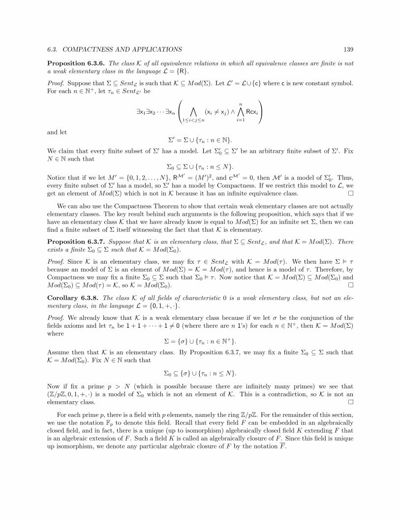
6.3. COMPACTNESS AND APPLICATIONS 139
Proposition 6.3.6. The class K of all equivalence relations in which all equivalence classes are finite is nota weak elementary class in the language L = {R}.
Proof. Suppose that Σ ⊆ SentL is such that K ⊆Mod(Σ). Let L′ = L∪{c} where c is new constant symbol.For each n ∈ N+, let τn ∈ SentL′ be
∃x1∃x2 · · · ∃xn
∧1≤i<j≤n
(xi 6= xj) ∧n∧i=1
Rcxi
and let
Σ′ = Σ ∪ {τn : n ∈ N}.We claim that every finite subset of Σ′ has a model. Let Σ′0 ⊆ Σ′ be an arbitrary finite subset of Σ′. FixN ∈ N such that
Σ0 ⊆ Σ ∪ {τn : n ≤ N}.Notice that if we let M ′ = {0, 1, 2, . . . , N}, RM
′= (M ′)2, and cM
′= 0, then M′ is a model of Σ′0. Thus,
every finite subset of Σ′ has a model, so Σ′ has a model by Compactness. If we restrict this model to L, weget an element of Mod(Σ) which is not in K because it has an infinite equivalence class.
We can also use the Compactness Theorem to show that certain weak elementary classes are not actuallyelementary classes. The key result behind such arguments is the following proposition, which says that if wehave an elementary class K that we have already know is equal to Mod(Σ) for an infinite set Σ, then we canfind a finite subset of Σ itself witnessing the fact that that K is elementary.
Proposition 6.3.7. Suppose that K is an elementary class, that Σ ⊆ SentL, and that K = Mod(Σ). Thereexists a finite Σ0 ⊆ Σ such that K = Mod(Σ0).
Proof. Since K is an elementary class, we may fix τ ∈ SentL with K = Mod(τ). We then have Σ � τbecause an model of Σ is an element of Mod(Σ) = K = Mod(τ), and hence is a model of τ . Therefore, byCompactness we may fix a finite Σ0 ⊆ Σ such that Σ0 � τ . Now notice that K = Mod(Σ) ⊆ Mod(Σ0) andMod(Σ0) ⊆Mod(τ) = K, so K = Mod(Σ0).
Corollary 6.3.8. The class K of all fields of characteristic 0 is a weak elementary class, but not an ele-mentary class, in the language L = {0, 1,+, ·}.
Proof. We already know that K is a weak elementary class because if we let σ be the conjunction of thefields axioms and let τn be 1 + 1 + · · ·+ 1 6= 0 (where there are n 1’s) for each n ∈ N+, then K = Mod(Σ)where
Σ = {σ} ∪ {τn : n ∈ N+}.Assume then that K is an elementary class. By Proposition 6.3.7, we may fix a finite Σ0 ⊆ Σ such thatK = Mod(Σ0). Fix N ∈ N such that
Σ0 ⊆ {σ} ∪ {τn : n ≤ N}.
Now if fix a prime p > N (which is possible because there are infinitely many primes) we see that(Z/pZ, 0, 1,+, ·) is a model of Σ0 which is not an element of K. This is a contradiction, so K is not anelementary class.
For each prime p, there is a field with p elements, namely the ring Z/pZ. For the remainder of this section,we use the notation Fp to denote this field. Recall that every field F can be embedded in an algebraicallyclosed field, and in fact, there is a unique (up to isomorphism) algebraically closed field K extending F thatis an algebraic extension of F . Such a field K is called an algebraically closure of F . Since this field is uniqueup isomorphism, we denote any particular algebraic closure of F by the notation F .
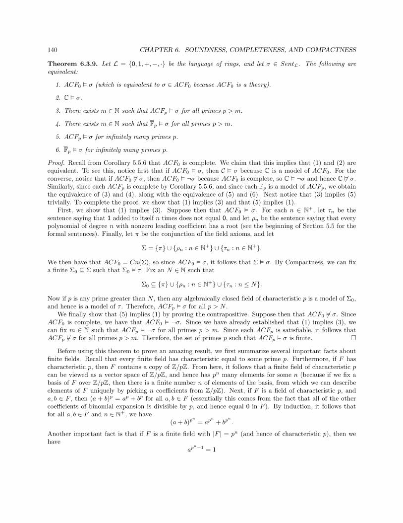
140 CHAPTER 6. SOUNDNESS, COMPLETENESS, AND COMPACTNESS
Theorem 6.3.9. Let L = {0, 1,+,−, ·} be the language of rings, and let σ ∈ SentL. The following areequivalent:
1. ACF0 � σ (which is equivalent to σ ∈ ACF0 because ACF0 is a theory).
2. C � σ.
3. There exists m ∈ N such that ACFp � σ for all primes p > m.
4. There exists m ∈ N such that Fp � σ for all primes p > m.
5. ACFp � σ for infinitely many primes p.
6. Fp � σ for infinitely many primes p.
Proof. Recall from Corollary 5.5.6 that ACF0 is complete. We claim that this implies that (1) and (2) areequivalent. To see this, notice first that if ACF0 � σ, then C � σ because C is a model of ACF0. For theconverse, notice that if ACF0 6� σ, then ACF0 � ¬σ because ACF0 is complete, so C � ¬σ and hence C 6� σ.Similarly, since each ACFp is complete by Corollary 5.5.6, and since each Fp is a model of ACFp, we obtainthe equivalence of (3) and (4), along with the equivalence of (5) and (6). Next notice that (3) implies (5)trivially. To complete the proof, we show that (1) implies (3) and that (5) implies (1).
First, we show that (1) implies (3). Suppose then that ACF0 � σ. For each n ∈ N+, let τn be thesentence saying that 1 added to itself n times does not equal 0, and let ρn be the sentence saying that everypolynomial of degree n with nonzero leading coefficient has a root (see the beginning of Section 5.5 for theformal sentences). Finally, let π be the conjunction of the field axioms, and let
Σ = {π} ∪ {ρn : n ∈ N+} ∪ {τn : n ∈ N+}.
We then have that ACF0 = Cn(Σ), so since ACF0 � σ, it follows that Σ � σ. By Compactness, we can fixa finite Σ0 ⊆ Σ such that Σ0 � τ . Fix an N ∈ N such that
Σ0 ⊆ {π} ∪ {ρn : n ∈ N+} ∪ {τn : n ≤ N}.
Now if p is any prime greater than N , then any algebraically closed field of characteristic p is a model of Σ0,and hence is a model of τ . Therefore, ACFp � σ for all p > N .
We finally show that (5) implies (1) by proving the contrapositive. Suppose then that ACF0 6� σ. SinceACF0 is complete, we have that ACF0 � ¬σ. Since we have already established that (1) implies (3), wecan fix m ∈ N such that ACFp � ¬σ for all primes p > m. Since each ACFp is satisfiable, it follows thatACFp 6� σ for all primes p > m. Therefore, the set of primes p such that ACFp � σ is finite.
Before using this theorem to prove an amazing result, we first summarize several important facts aboutfinite fields. Recall that every finite field has characteristic equal to some prime p. Furthermore, if F hascharacteristic p, then F contains a copy of Z/pZ. From here, it follows that a finite field of characteristic pcan be viewed as a vector space of Z/pZ, and hence has pn many elements for some n (because if we fix abasis of F over Z/pZ, then there is a finite number n of elements of the basis, from which we can describeelements of F uniquely by picking n coefficients from Z/pZ). Next, if F is a field of characteristic p, anda, b ∈ F , then (a + b)p = ap + bp for all a, b ∈ F (essentially this comes from the fact that all of the othercoefficients of binomial expansion is divisible by p, and hence equal 0 in F ). By induction, it follows thatfor all a, b ∈ F and n ∈ N+, we have
(a+ b)pn
= apn
+ bpn
.
Another important fact is that if F is a finite field with |F | = pn (and hence of characteristic p), then wehave
apn−1 = 1

6.3. COMPACTNESS AND APPLICATIONS 141
for all nonzero a ∈ F by Lagrange’s Theorem (because F\{0} is a finite group of order pn − 1 undermultiplication). Therefore, we have
apn
= a
for all a ∈ F , including 0. With all of this in mind, we have the following fact.
Proposition 6.3.10. Let p be prime. Every finitely generated subfield of Fp is finite.
Proof. Let p be an arbitrary prime. For each n ∈ N+, let Kn = {a ∈ Fp : apn
= a}, and notice that Kn is theset of roots of xp
n − x in Fp. Since Fp is algebraically closed, we know that xpn − x splits in Fp. Notice that
xpn − x is a separable polynomial because it has formal derivative equal to −1, which is trivially relatively
prime to xpn − x. Therefore, the roots of xp
n − x in Fp are distinct, and hence |Kn| = pn. Furthermore, wehave that each Kn is closed under addition and multiplication because if a, b ∈ Kn, then
(a+ b)pn
= apn
+ bpn
= a+ b
from above, and(ab)p
n
= apn
bpn
= ab.
Notice that −1 ∈ Kn because we have (−1)pn
= −1 whenever p is odd, and (−1)pn
= 1 = −1 when p = 2.Since Kn is closed under multiplication, it follows that if a ∈ Kn is arbitrary, then −a = (−1) · a ∈ Kn.Finally, if if a ∈ K is nonzero, then
(a−1)pn
= (apn
)−1 = a−1,
so Kn is closed under multiplicative inverses (of nonzero elements). Therefore, Kn is a subfield of Fp withpn elements. Moreover, if L is an arbitrary subfield of Fp with pn many elements, then ap
n
= a for all a ∈ Lfrom above, so L ⊆ K, and hence L = K because L and K are finite sets of the same cardinality. In otherwords, Kn is the unique subfield of Fp with pn elements.
Next, let we claim that if d | n, then Kd ⊆ Kn. To see this, let a ∈ Kd be arbitrary. We then have
apd
= a, so
ap2·d
= (apd
)pd
= apd
= a
henceap
3·d= (ap
2·d)pd
= apd
= a.
By a simple induction, it follows that apmd
= a for all m ∈ N+. Thus, if d | n, then Kd ⊆ Kn.Let K =
⋃n∈NKn. We claim that K = Fp. We clearly have that K ⊆ Fp. To show equality, it suffices
to show that K itself is algebraically closed. Let f(x) ∈ K[x] be an arbitrary nonconstant polynomial, andwrite f(x) = amx
m + am−1xm−1 + · · ·+ a1x+ a0 where each ai ∈ K. Using the fact that K =
⋃n∈NKn and
that Kd ⊆ Kn whenever d | n, there exists N ∈ N+ such that ai ∈ KN for all i (by taking a least commonmultiple). Now f(x) ∈ KN [x] ⊆ Fp[x], so since Fp is algebraically closed, we know that it has some rootα of f(x). We now have KN ⊆ KN (α) ⊆ Fp, and that KN (α) is a finite extension of KN . Since KN is afinite field, and KN (α) is a finite extension of KN , the field KN (α) is a finite subfield of Fp. Since everyfinite subfield of Fp equals some Kn, we conclude that KN (α) ⊆ K, and hence α ∈ K. Therefore, everypolynomial over K has a root in K, and hence K is algebraically closed. It follows that K = Fp.
We now prove the result. Let a1, a2, . . . , am ∈ Fp be arbitrary. Since Fp = K, we have a1, a2, . . . , am ∈ K.By taking a least common multiple, we can fix N ∈ N+ such that a1, a2, . . . , am ∈ KN . We then have thatthe subfield of Fp generated by a1, a2, . . . , am is a subfield of KN , and hence is finite.
Given a field F , each polynomial in F [x] determines a function from F to F via evaluation. Similarly,an element of F [x1, x2, . . . , xn], i.e. a polynomial of several variables, determines a function from Fn to Fvia evaluation. By putting several such polynomial functions (in the same number of variables) together,we can define polynomial functions from Fn to Fm. For example, if f1(x, y) = x2y + 5x and f2(x, y) =x5y − 3xy2 + 7y3, then f(x, y) = (f1(x, y), f2(x, y)) can be viewed as a polynomial function from Q2 to Q2
(or really from F 2 to F 2 for any field F ).

142 CHAPTER 6. SOUNDNESS, COMPLETENESS, AND COMPACTNESS
Theorem 6.3.11 (Ax-Grothendieck). Every injective polynomial map from Cn to Cn is surjective.
Proof. Let L = {0, 1,+,−, ·} be the language of rings. Notice that given any n, d ∈ N+, we can write asentence σn,d ∈ SentL expressing that every injective polynomial map from Fn to Fn, where each polynomialhas degree at most d, is surjective. We want to show that C � σn,d for all n, d ∈ N+. By Theorem 6.3.9, itsuffices to show that Fp � σn,d for all primes p and all n, d ∈ N+. Thus, it suffices to show that for all primes
p and all n ∈ N+, every injective polynomial map from Fnp to Fnp is surjective.
Let p, n ∈ N+ be arbitrary with p prime. Let f : Fnp → Fnp be an arbitrary injective polynomial map,
and let (b1, b2, . . . , bn) ∈ Fnp be arbitrary. We need to show that there exists (a1, a2, . . . , an) ∈ Fnp with
f(a1, a2, . . . , an) = (b1, b2, . . . , bn). Let f1, f2, . . . , fn ∈ Fp[x1, x2, . . . , xn] be such that f = (f1, f2, . . . , fn),and let C be the finite set of coefficients appearing in f1, f2, . . . , fn. Let K be the subfield of Fp generated byC ∪ {b1, b2, . . . , bn} and notice that K is a finite field by Proposition 6.3.10. Now f � Kn maps Kn into Kn
and is injective, so must be surjective because Kn is finite. Thus, there exists (a1, a2, . . . , an) ∈ Kn ⊆ Fnpsuch that f(a1, a2, . . . , an) = (b1, b2, . . . , bn).
6.4 Random Graphs
Throughout this section, we work in the language L = {R} where R is binary relation symbol. We considerloopless undirected graphs, which we view as L-structures that are models of {∀x¬Rxx,∀x∀y(Rxy→ Ryx)}.
Definition 6.4.1. For each n ∈ N+, let Gn be the set of of all models of {∀x¬Rxx,∀x∀y(Rxy→ Ryx)} withuniverse [n].
Definition 6.4.2. For each A ⊆ Gn, we let
Prn(A) =|A||Gn|
.
For each σ ∈ SentL, we let
Prn(σ) =|{M ∈ Gn :M � σ}|
|Gn|.
We use the suggestive Pr because we think of constructing a graph randomly by flipping a fair coin foreach 2-element subset {i, j} of [n] to determine whether or not there is an edge linking them. In this context,Prn(A) is the probability the graph so constructed with vertex set [n] is an element of A. Notice that if Aand B are both subsets of Gn, then we trivially have |A ∪ B| ≤ |A|+ |B|, and hence
Prn(A ∪ B) =|A ∪ B||Gn|
≤ |A|+ |B||Gn|
≤ |A||Gn|
+|B||Gn|
= Prn(A) + Prn(B).
More generally if A1,A2, . . . ,Ak are all subsets of Gn, then
Prn(A1 ∪ A2 ∪ · · · ∪ Ak) ≤ Prn(A1) + Prn(A2) + · · ·+ Prn(Ak).

6.4. RANDOM GRAPHS 143
Notice that if A ⊆ B ⊆ Gn, then
Prn(A) =|A||Gn|
≤ |B||Gn|
= Prn(B)
and for any A ⊆ Gn, we have
Prn(Gn\A) = 1− Prn(A).
Now given given two distinct 2-element subsets {i, j} and {i′, j′} of {1, 2, . . . , n}, the question of whetherthere is an edge linking i and j and the question of whether there is an edge linking i′ and j′ is independent.More formally, if
A1 = {M ∈ Gn : (i, j) ∈ RM}
and
A2 = {M ∈ Gn : (i′, j′) ∈ RM},
then we have
Prn(A1 ∩ A2) =1
4=
1
2· 1
2= Prn(A1) · Prn(A2).
More generally, suppose that we have sets E1, E2, . . . , Ek, where each Ei is set of 2-element subsets of [n].Suppose that we fix choices for whether each pair in Ei should be in the graph or not, and let Ai be the subsetof Gn consisting of those edges that meet the requirements for the edges in Ei. If the sets E1, E2, . . . , Ek arepairwise disjoint, then
Prn(A1 ∩ A2 ∩ · · · ∩ Ak) = Prn(A1) · Prn(A2) · · ·Prn(Ak).
In other words, the events saying that the edges in each of Ei behave according to a specified pattern aremutually independent when the Ei are pairwise disjoint.
For example, suppose that σ is the sentence
∃x∃y∃z(Rxy ∧ Ryz ∧ Rzx)
saying that the graph has a triangle. We want to understand Prn(σ). Determining the exact values forvarious n is difficult, but we can classify the long term behavior as n gets large. To see this, let n ∈ N+ bearbitrary. Consider partitioning the n vertices of [n] into bn3 c many set of size 3 (with perhaps 1 or 2 verticesleft over) by considering the sets {1, 2, 3}, then {4, 5, 6}, etc. Now for any one of these sets, the probabilitythat the vertices in the set forms a triangle is ( 1
2 )3 = 18 , so the probability that the vertices in a set does not
form a triangle is 1 − 18 = 7
8 . Since these events are mutually independent (as the corresponding potentialedge sets are disjoint), the probability that none of these families forms a triangle equals(
7
8
)bn3 c.
Therefore, the probability that there is no triangle, which is Prn(¬σ), satisfies the following inequality:
Prn(¬σ) ≤(
7
8
)bn3 c≤(
7
8
)n3
.

144 CHAPTER 6. SOUNDNESS, COMPLETENESS, AND COMPACTNESS
It follows that
Prn(σ) = 1− Prn(¬σ)
≥ 1−(
7
8
)n3
.
Since
limn→∞
(1−
(7
8
)n3
)= 1− 0 = 1,
and we trivially have Prn(σ) ≤ 1 for all n ∈ N+, we conclude that limn→∞
Prn(σ) = 1. In other words, when
n is large, a randomly constructed graph on [n] will almost surely have a triangle.For another example, consider the sentence
∀x1∀x2(¬(x1 = x2)→ ∃z(¬(z = x1) ∧ ¬(z = x2) ∧ Rx1z ∧ Rx2z))
saying that whenever we have two distinct vertices, we can find a common neighbor. Let n ∈ N with n ≥ 3be arbitrary. Consider arbitrary distinct a1, a2 ∈ [n]. For each c ∈ [n] distinct from the a1 and a2, let
Ac = {M ∈ Gn : c is adjacent to both a1 and a2},
so thatGn\Ac = {M ∈ Gn : c is not adjacent to at least one of a1 or a2}.
For each such c, we have Prn(Ac) = (12 )2 = 1
4 , so Prn(Gn\Ac) = 1− 14 = 3
4 . As we vary c through the n− 2other vertices, the corresponding events Gn\Ac are mutually independent, so the probability that no c is acommon neighbor for this particular pair {a1, a2} equals
Prn(⋂c
(Gn\Ac)) =∏c
Prn(Gn\Ac) =
(3
4
)n−2
.
Now there are(n2
)possible pairs of distinct vertices a1 and a2, so the probability that there exists such a
pair with no common neighbor is
Prn(¬σ) ≤(n
2
)·(
3
4
)n−2
=n(n− 1)
2·(
3
4
)n−2
.
Since
limn→∞
n(n− 1)
2·(
3
4
)n−2
= 0
(see the proof of Proposition 6.4.5), it follows that limn→∞
Pr(¬σ) = 0. Using the fact that Prn(σ) = 1 −Prn(¬σ), we conclude that lim
n→∞Prn(σ) = 1.
We aim to prove the following result, originally proven by Glebskii, Kogan, Liagonkii, and Talanov, butalso independently by Fagin.
Theorem 6.4.3. For all σ ∈ SentL, either limn→∞
Prn(σ) = 1 or limn→∞
Prn(σ) = 0.
The key step in proving this result is generalizing the last example.

6.4. RANDOM GRAPHS 145
Definition 6.4.4. For each r, s ∈ N with max{r, s} > 0, let σr,s be the sentence
∀x1∀x2 · · · ∀xr∀y1∀y2 · · · ∀ys(∧
1≤i<j≤r
(xi 6= xj) ∧∧
1≤i<j≤s
(yi 6= yj) ∧r∧
i=1
s∧j=1
(xi 6= yj)
→ ∃z(
r∧i=1
(z 6= xi) ∧s∧
j=1
(z 6= yj) ∧r∧
i=1
Rxiz ∧s∧
j=1
¬Ryjz))
If s = 0, we simply omit all quantifiers and conjuncts mentioning a yj. Similarly, if r = 0, we simply omitall quantifiers and conjuncts mentioning a xi.
Intuitively, a graph is model of σr,s if it has the property that whenever A and B are disjoint sets ofvertices with |A| = r and |B| = s, we can always find a vertex u /∈ A∪B that is adjacent to every element ofA, but not adjacent to any element of B. Peter Winkler has called the statements σr,s the Alice’s Restaurantaxioms, references Arlo Guthrie’s story/song containing the line “You can get anything you want at Alice’sRestaurant”.
Proposition 6.4.5. For all r, s ∈ N with max{r, s} > 0, we have limn→∞
Prn(σr,s) = 1.
Proof. Let r, s ∈ N be arbitrary with max{r, s} > 0. Let n ∈ N be arbitrary with n > r + s. Considerarbitrary disjoint subsets U and W of [n] with |U | = r and |W | = s. For each c ∈ [n]\(U ∪W ), let
Ac = {M ∈ Gn : c is adjacent to each element of U and to no element of W}
For each such c, we have Prn(Ac) = 12r+s , so Prn(Gn\Ac) = 1 − 1
2r+s . As we vary c through the n − r − svertices in [n]\(U ∪W ), the corresponding events Gn\Ac are mutually independent, so the probability thatno c works for this choice of U and W equals(
1− 1
2r+s
)n−r−s.
Now there are(nr
)·(n−rs
)possible choices for the sets U and W , so
Prn(¬σr,s) ≤(n
r
)(n− rs
)(1− 1
2r+s
)n−r−s≤ nr · ns ·
(1− 1
2r+s
)n−r−s=
(1− 1
2r+s
)−r−s· nr+s ·
(1− 1
2r+s
)n=
(1− 1
2r+s
)−r−s· nr+s ·
(2r+s − 1
2r+s
)n=
(1− 1
2r+s
)−r−s· nr+s(
2r+s
2r+s−1
)nNow we use the fact that if k ∈ N+ and r ∈ R with r > 1, then
limn→∞
nk
rn= 0
(i.e. that any exponential eventually dominates any polynomial) to conclude that limn→∞
Prn(¬σr,s) = 0.
Therefore limn→∞
Prn(σr,s) = 1.
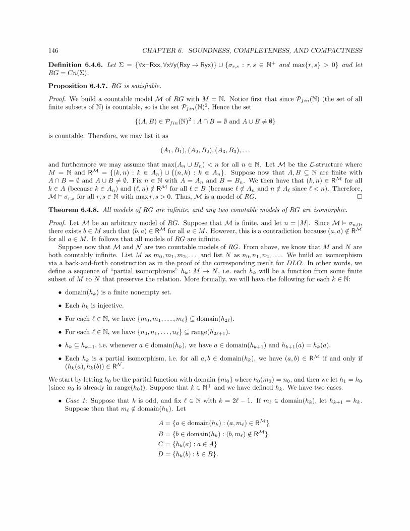
146 CHAPTER 6. SOUNDNESS, COMPLETENESS, AND COMPACTNESS
Definition 6.4.6. Let Σ = {∀x¬Rxx,∀x∀y(Rxy→ Ryx)} ∪ {σr,s : r, s ∈ N+ and max{r, s} > 0} and letRG = Cn(Σ).
Proposition 6.4.7. RG is satisfiable.
Proof. We build a countable model M of RG with M = N. Notice first that since Pfin(N) (the set of allfinite subsets of N) is countable, so is the set Pfin(N)2, Hence the set
{(A,B) ∈ Pfin(N)2 : A ∩B = ∅ and A ∪B 6= ∅}
is countable. Therefore, we may list it as
(A1, B1), (A2, B2), (A3, B3), . . .
and furthermore we may assume that max(An ∪ Bn) < n for all n ∈ N. Let M be the L-structure whereM = N and RM = {(k, n) : k ∈ An} ∪ {(n, k) : k ∈ An}. Suppose now that A,B ⊆ N are finite withA ∩ B = ∅ and A ∪ B 6= ∅. Fix n ∈ N with A = An and B = Bn. We then have that (k, n) ∈ RM for allk ∈ A (because k ∈ An) and (`, n) /∈ RM for all ` ∈ B (because ` /∈ An and n /∈ A` since ` < n). Therefore,M � σr,s for all r, s ∈ N with max r, s > 0. Thus, M is a model of RG.
Theorem 6.4.8. All models of RG are infinite, and any two countable models of RG are isomorphic.
Proof. Let M be an arbitrary model of RG. Suppose that M is finite, and let n = |M |. Since M � σn,0,there exists b ∈M such that (b, a) ∈ RM for all a ∈M . However, this is a contradiction because (a, a) /∈ RM
for all a ∈M . It follows that all models of RG are infinite.Suppose now thatM and N are two countable models of RG. From above, we know that M and N are
both countably infinite. List M as m0,m1,m2, . . . and list N as n0, n1, n2, . . . . We build an isomorphismvia a back-and-forth construction as in the proof of the corresponding result for DLO. In other words, wedefine a sequence of “partial isomorphisms” hk : M → N , i.e. each hk will be a function from some finitesubset of M to N that preserves the relation. More formally, we will have the following for each k ∈ N:
• domain(hk) is a finite nonempty set.
• Each hk is injective.
• For each ` ∈ N, we have {m0,m1, . . . ,m`} ⊆ domain(h2`).
• For each ` ∈ N, we have {n0, n1, . . . , n`} ⊆ range(h2`+1).
• hk ⊆ hk+1, i.e. whenever a ∈ domain(hk), we have a ∈ domain(hk+1) and hk+1(a) = hk(a).
• Each hk is a partial isomorphism, i.e. for all a, b ∈ domain(hk), we have (a, b) ∈ RM if and only if(hk(a), hk(b)) ∈ RN .
We start by letting h0 be the partial function with domain {m0} where h0(m0) = n0, and then we let h1 = h0
(since n0 is already in range(h0)). Suppose that k ∈ N+ and we have defined hk. We have two cases.
• Case 1: Suppose that k is odd, and fix ` ∈ N with k = 2` − 1. If m` ∈ domain(hk), let hk+1 = hk.Suppose then that m` /∈ domain(hk). Let
A = {a ∈ domain(hk) : (a,m`) ∈ RM}B = {b ∈ domain(hk) : (b,m`) /∈ RM}C = {hk(a) : a ∈ A}D = {hk(b) : b ∈ B}.

6.4. RANDOM GRAPHS 147
Since domain(hk) is finite, we have that A and B are finite disjoint subsets of M with A ∪ B =domain(hk). Since hk is injective, we have that C and D are disjoint subsets of N with C ∪ D =range(hk), and that |A| = |C| and |B| = |D|. Now N is model of RG and C ∩D = ∅, so we can fixw ∈ N\(C ∪D) such that (c, w) ∈ RN for all c ∈ C and (d,w) /∈ RN for all d ∈ D. We now extendhk to hk+1 by letting hk+1(m`) = w. It is straightforward to check that if hk satisfies all of the aboveconditions, then hk+1 also satisfies all of the necessary conditions.
• Case 2: Suppose that k is even, and fix ` ∈ N with k = 2`. If n` ∈ range(hk), let hk+1 = hk. Supposethen that n` /∈ range(hk). Let
C = {c ∈ range(hk) : (c, n`) ∈ RN }D = {d ∈ range(hk) : (d, n`) /∈ RN }A = {a ∈ domain(hk) : hk(a) ∈ C}B = {b ∈ domain(hk) : hk(b) ∈ D}.
Since domain(hk) is finite, we have that range(hk) is finite, and so C and D are finite disjoint subsetsof N with C ∪D = range(hk). Since hk is injective, we have that A and B are disjoint subsets of Mwith A ∪B = domain(hk), and that |A| = |C| and |B| = |D|. Now M is model of RG and A ∩B = ∅,so we can fix u ∈ M\(A ∪ B) such that (a, u) ∈ RM for all a ∈ A and (b, u) /∈ RM for all b ∈ B. Wenow extend hk to hk+1 by letting hk+1(u) = n`. It is straightforward to check that if hk satisfies all ofthe above conditions, then hk+1 also satisfies all of the necessary conditions.
Now define h : M → N by letting h(m`) = h2`(m`) for each ` ∈ N. Using the second through fifth conditionson the hk, we conclude that h is a bijection. Now let a, b ∈ M be arbitrary. Fix k, ` ∈ N with a = mk andb = m`. Let t = max{k, `}. Since a, b ∈ domain(h2t), we have (a, b) ∈ RM if and only if (h2t(a), h2t(b)) ∈ RM,which by fifth condition on the hk is if and only if (h(a), h(b)) ∈ RM. Therefore, h is an isomorphism.
Corollary 6.4.9. RG is a complete theory.
Proof. Immediate from the Countable Los-Vaught Test.
Theorem 6.4.10. Let τ ∈ SentL.
1. If τ ∈ RG, then limn→∞
Prn(τ) = 1.
2. If τ /∈ RG, then limn→∞
Prn(τ) = 0.
Proof.
1. Let τ ∈ RG be arbitrary. We then have Σ � τ , so by Compactness we may fix N ∈ N such that
{∀x¬Rxx,∀x∀y(Rxy→ Ryx)} ∪ {σr,s : r, s ≤ N} � τ.
We then have that if M∈ Gn is such that M � ¬τ , then
M �∨
0≤r,s≤N,max{r,s}>0
¬σr,s
Hence for every n ∈ N we have
Prn(¬τ) ≤∑
0≤r,s≤N,max{r,s}>0
Prn(¬σr,s)
Since limn→∞
Prn(¬σr,s) = 0 for each fixed choice of r and s, and since we have a finite sum, we conclude
that limn→∞
Prn(¬τ) = 0. Therefore, limn→∞
Prn(τ) = 1.

148 CHAPTER 6. SOUNDNESS, COMPLETENESS, AND COMPACTNESS
2. Suppose that τ /∈ RG. Since RG is complete, it follows that ¬τ ∈ RG. Thus, limn→∞
Prn(¬τ) = 1 by
part 1, and hence limn→∞
Prn(τ) = 0.
With this background, the theorem that we want to prove is now immediate.
Proof of Theorem 6.4.3. Apply the previous theorem together with the fact that RG is complete.
6.5 Nonstandard Models of Arithmetic
Throughout this section, we work in the language L = {0, 1, <,+, ·}, where 0, 1 are constant symbols, < isa binary relation symbol, and +, · are binary function symbols. We also let N = (N, 0, 1, <,+, ·) where thesymbol 0 is interpreted as the “real” 0, the symbol + is interpreted as “real” addition, etc. Be careful todistinguish when + means the symbol in the language L, and when it mean the addition function on N. Ourfirst question is whether Th(N) completely determines the model N.
Question 6.5.1. Are all models of Th(N) isomorphic to N?
Using Proposition 6.3.4, we can immediately give a negative answer to this question because there is anuncountable model of Th(N), and an uncountable model is certainly not isomorphic to N. What would sucha model look like? In order to answer this question, let’s think a little about the kinds of sentences that arein Th(N).
Definition 6.5.2. For each n ∈ N, we define a term n ∈ TermL as follows. Let 0 = 0 and let 1 = 1. Nowdefine n recursively by letting n+ 1 = n+ 1 for each n ≥ 1. Notice here that the 1 and the + in n+ 1 meansthe actual number 1 and the actual addition function, whereas the 1 and + in n+ 1 mean the symbols 1 and+ in our language L. Thus, for example, 2 is the term 1 + 1 and 3 is the term (1 + 1) + 1.
Definition 6.5.3. Let M be an L-structure. We know that given any t ∈ TermL containing no variables, tcorresponds to an element of M given by s(t) for some (any) variable assignment s : V ar →M . We denotethis value by tM.
Notice that nN = n for all n ∈ N be a simple induction. Here are some important examples of somesentences that are true in N, and hence are elements of Th(N):
1. 2 + 2 = 4 and in general m+ n = m+ n and m · n = m · n for all m,n ∈ N.
2. ∀x∀y(x + y = y + x).
3. ∀x(¬(x = 0)→ ∃y(y + 1 = x)).
4. ∀x¬(∃y((x < y) ∧ (y < x + 1))).
5. For each ϕ(x) ∈ FormL, the sentence
(ϕ0x ∧ ∀x(ϕ→ ϕx+1
x ))→ ∀xϕ
expressing that induction holds on the subset of N defined by ϕ(x) is in Th(N). We often write thissentence in the following informal way:
(ϕ(0) ∧ ∀x(ϕ(x)→ ϕ(x + 1)))→ ∀xϕ.
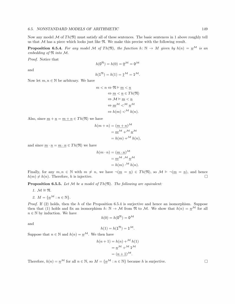
6.5. NONSTANDARD MODELS OF ARITHMETIC 149
Now any modelM of Th(N) must satisfy all of these sentences. The basic sentences in 1 above roughly tellus that M has a piece which looks just like N. We make this precise with the following result.
Proposition 6.5.4. For any model M of Th(N), the function h : N → M given by h(n) = nM is anembedding of N into M.
Proof. Notice thath(0N) = h(0) = 0M = 0M
andh(1N) = h(1) = 1M = 1M.
Now let m,n ∈ N be arbitrary. We have
m < n⇔ N � m < n
⇔ m < n ∈ Th(N)
⇔M � m < n
⇔ mM <M nM
⇔ h(m) <M h(n).
Also, since m+ n = m+ n ∈ Th(N) we have
h(m+ n) = (m+ n)M
= mM +M nM
= h(m) +M h(n),
and since m · n = m · n ∈ Th(N) we have
h(m · n) = (m · n)M
= mM ·M nM
= h(m) ·M h(n).
Finally, for any m,n ∈ N with m 6= n, we have ¬(m = n) ∈ Th(N), so M � ¬(m = n), and henceh(m) 6= h(n). Therefore, h is injective.
Proposition 6.5.5. Let M be a model of Th(N). The following are equivalent:
1. M∼= N.
2. M = {nM : n ∈ N}.Proof. If (2) holds, then the h of the Proposition 6.5.4 is surjective and hence an isomorphism. Supposethen that (1) holds and fix an isomorphism h : N → M from N to M. We show that h(n) = nM for alln ∈ N by induction. We have
h(0) = h(0N) = 0M
andh(1) = h(1N) = 1M.
Suppose that n ∈ N and h(n) = nM. We then have
h(n+ 1) = h(n) +M h(1)
= nM +M 1M
= (n+ 1)M.
Therefore, h(n) = nM for all n ∈ N, so M = {nM : n ∈ N} because h is surjective.

150 CHAPTER 6. SOUNDNESS, COMPLETENESS, AND COMPACTNESS
Definition 6.5.6. A nonstandard model of arithmetic is a model M of Th(N) such that M 6∼= N.
We’ve already seen that there are nonstandard models of arithmetic by cardinality considerations, butwe can also build countable nonstandard models of arithmetic using the Compactness Theorem and theCountable Lowenheim-Skolem Theorem.
Theorem 6.5.7. There exists a countable nonstandard model of arithmetic.
Proof. Let L′ = L ∪ {c} where c is a new constant symbol. Consider the following set of L′-sentences:
Σ′ = Th(N) ∪ {c 6= n : n ∈ N}
Notice that every finite subset of Σ′ is satisfiable (by taking N and interpreting c large enough), so Σ′
is satisfiable by the Compactness Theorem. Furthermore, by the Countable Lowenheim-Skolem Theorem(notice that L′ is countable), there is a countable model M of Σ′. Restricting this model to the originallanguage L, we may use Proposition 6.5.5 to conclude thatM is a countable nonstandard model of arithmetic.
For the rest of this section, we work with a structure M that is a nonstandard model of arithmetic. Asmentioned, anything that we can express in the first-order language of L that is true of N is in Th(N), andhence is true in M. For example, we have the following.
Proposition 6.5.8. Let M be a nonstandard model of arithmetic.
• +M is associative on M .
• +M is commutative on M .
• <M is a linear ordering on M .
• For all a ∈M with a 6= 0M, there exists b ∈M with a+ 1M = b.
Proof. Consider the following sentences:
• ∀x∀y∀z(x + (y + z) = (x + y) + x)
• ∀x∀y(x + y = y + x)
• ∀x∀y(x < y ∨ y < x ∨ x = y)
• ∀x(x 6= 0→ ∃y(y + 1 = x))
Each of these sentences is true in N, so is an element of Th(N), and hence is true in M.
Since we already know that N naturally embeds in M, and it gets tiresome to write +M, ·M, and <M,we’ll abuse notation by using just +, ·, and < to also denote the interpretations inM. Thus, these symbolsnow have three different meanings, depending on context: as formal symbols in our language, as the normalfunctions and relations in N, and as their interpretations in M.
Definition 6.5.9. Let M be a nonstandard model of arithmetic. We let Mfin = {nM : n ∈ N} and we callMfin the set of finite elements of M. We also let Minf = M\Mfin and we call Minf the set of infiniteelements of M.
The following proposition justifies our choice of name.
Proposition 6.5.10. Let M be a nonstandard model of arithmetic, and let a ∈ Minf . For any n ∈ N, wehave nM < a.

6.5. NONSTANDARD MODELS OF ARITHMETIC 151
Proof. For each n ∈ N, the sentence
∀x(x < n→n−1∨i=0
(x = i))
is in Th(N), and hence true in M. Since a ∈Minf , we have a 6= nM for all n ∈ N. Now given an arbitraryn ∈ N, we have that a 6< nM because the above sentence is true in M. Since < is a linear ordering on Mand a 6= nM for each n ∈ N, we conclude that nM < a for all n ∈ N.
Definition 6.5.11. LetM be a nonstandard model of arithmetic. Define a relation ∼ on M by letting a ∼ bif there exists n ∈ N such that either a+ nM = b or b+ nM = a.
In other words, we let a ∼ b if a and b are “finitely” far apart. Notice that if there exists n ∈ N witha+ nM = b, then we must have a ≤ b in M, because the sentence ∀x∀y((x = x + y) ∨ (x < x + y)) is true inN.
Proposition 6.5.12. If M be a nonstandard model of arithmetic, then ∼ is an equivalence relation on M .
Proof. ∼ is clearly reflexive and symmetric by definition. Let a, b, c ∈M be arbitrary such that both a ∼ band b ∼ c.
• Case 1: Suppose that we can fix m,n ∈ N with a+mM = b and b+ nM = c. We then have
a+ (m+ n)M = a+ (mM + nM) (by Proposition 6.5.4)
= (a+mM) + nM (since + is associative on M)
= b+ nM
= c,
so a ∼ c.
• Case 2: Suppose that we can fix m,n ∈ N with a+mM = b and c+ nM = b.
– Subcase 1: Suppose that m ≤ n. Let k = n−m ∈ N. We then have
(c+ kM) +mM = c+ (kM +mM) (since + is associative on M)
= c+ (k +m)M (by Proposition 6.5.4)
= c+ nM
= b
= a+mM.
Now ∀x∀y∀z(x + z = y + z→ x = y) is in Th(N), so is true in M. Therefore, we must havec+ kM = a, so a ∼ c.
– Subcase 2: Suppose that m > n. Let k = n −m ∈ N. Following the argument in Subcase 1, itfollows that a+ kM = c, so a ∼ c.
• The other two cases are similar.
Definition 6.5.13. Let M be a nonstandard model of arithmetic, and let a, b ∈ M . We write a � b tomean that a < b and a 6∼ b.
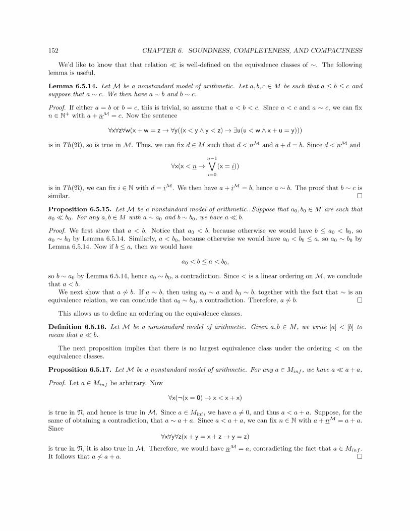
152 CHAPTER 6. SOUNDNESS, COMPLETENESS, AND COMPACTNESS
We’d like to know that that relation � is well-defined on the equivalence classes of ∼. The followinglemma is useful.
Lemma 6.5.14. Let M be a nonstandard model of arithmetic. Let a, b, c ∈ M be such that a ≤ b ≤ c andsuppose that a ∼ c. We then have a ∼ b and b ∼ c.
Proof. If either a = b or b = c, this is trivial, so assume that a < b < c. Since a < c and a ∼ c, we can fixn ∈ N+ with a+ nM = c. Now the sentence
∀x∀z∀w(x + w = z→ ∀y((x < y ∧ y < z)→ ∃u(u < w ∧ x + u = y)))
is in Th(N), so is true in M. Thus, we can fix d ∈M such that d < nM and a+ d = b. Since d < nM and
∀x(x < n→n−1∨i=0
(x = i))
is in Th(N), we can fix i ∈ N with d = iM. We then have a+ iM = b, hence a ∼ b. The proof that b ∼ c issimilar.
Proposition 6.5.15. Let M be a nonstandard model of arithmetic. Suppose that a0, b0 ∈ M are such thata0 � b0. For any a, b ∈M with a ∼ a0 and b ∼ b0, we have a� b.
Proof. We first show that a < b. Notice that a0 < b, because otherwise we would have b ≤ a0 < b0, soa0 ∼ b0 by Lemma 6.5.14. Similarly, a < b0, because otherwise we would have a0 < b0 ≤ a, so a0 ∼ b0 byLemma 6.5.14. Now if b ≤ a, then we would have
a0 < b ≤ a < b0,
so b ∼ a0 by Lemma 6.5.14, hence a0 ∼ b0, a contradiction. Since < is a linear ordering on M, we concludethat a < b.
We next show that a 6∼ b. If a ∼ b, then using a0 ∼ a and b0 ∼ b, together with the fact that ∼ is anequivalence relation, we can conclude that a0 ∼ b0, a contradiction. Therefore, a 6∼ b.
This allows us to define an ordering on the equivalence classes.
Definition 6.5.16. Let M be a nonstandard model of arithmetic. Given a, b ∈ M , we write [a] < [b] tomean that a� b.
The next proposition implies that there is no largest equivalence class under the ordering < on theequivalence classes.
Proposition 6.5.17. Let M be a nonstandard model of arithmetic. For any a ∈Minf , we have a� a+ a.
Proof. Let a ∈Minf be arbitrary. Now
∀x(¬(x = 0)→ x < x + x)
is true in N, and hence is true in M. Since a ∈ Minf , we have a 6= 0, and thus a < a+ a. Suppose, for thesame of obtaining a contradiction, that a ∼ a+ a. Since a < a+ a, we can fix n ∈ N with a+ nM = a+ a.Since
∀x∀y∀z(x + y = x + z→ y = z)
is true in N, it is also true in M. Therefore, we would have nM = a, contradicting the fact that a ∈Minf .It follows that a 6∼ a+ a.

6.5. NONSTANDARD MODELS OF ARITHMETIC 153
Lemma 6.5.18. Let M be a nonstandard model of arithmetic. For all a ∈M , one of the following holds:
1. There exists b ∈M such that a = 2M · b.
2. There exists b ∈M such that a = 2M · b+ 1M.
Proof. The sentence∀x∃y(x = 2 · y ∨ x = 2 · y + 1)
is in Th(N), and hence is true in M.
Proposition 6.5.19. LetM be a nonstandard model of arithmetic. For any a ∈Minf , there exists b ∈Minf
with b� a.
Proof. Let a ∈Minf be arbitrary. Using Lemma 6.5.18, we have two cases:
• Case 1: Suppose first that there exists b ∈ M such that a = 2M · b, and fix such a b. We then havea = b + b (because ∀x(2 · x = x + x) is in Th(N)). Notice that b /∈ Mfin because otherwise we wouldhave a ∈Mfin. Using Proposition 6.5.17, we conclude that b� b+ b = a.
• Case 2: Suppose now that there exists b ∈M such that a = 2M ·b+1M. We then have a = (b+b)+1M
because ∀x(2 · x + 1 = (x + x) + 1) is in Th(N). Notice that b /∈Mfin because otherwise we would havea ∈Mfin. By Proposition 6.5.17, we know that b� b+ b. Now b+ b ∼ b+ b+1M, so b� b+ b+1 = aby Proposition 6.5.15.
Proposition 6.5.20. Let M be a nonstandard model of arithmetic. For any a, b ∈Minf with a� b, thereexists c ∈Minf with a� c� b.
Proof. Let a, b ∈Minf with a� b be arbitrary. We again have two cases:
• Case 1: Suppose first that there exists c ∈ M with a + b = 2M · c, and fix such a c. We then havea+ b = c+ c. Since
∀x∀y∀z((x < y ∧ x + y = z + z)→ (x < z ∧ z < y))
is in Th(N) it follows that a < c < b. Thus, we need only show that a 6∼ c and c 6∼ b.Suppose that a ∼ c. Since a < c, we can fix n ∈ N with a+ nM = c. We then have that
a+ b = c+ c
= a+ a+ (2n)M.
Since additive cancellation is expressible as a first-order sentence that is true in N, we conclude thatb = a+ (2n)M, contradicting the fact that a� b. Therefore a 6∼ c.Suppose that c ∼ b. Since c < b, we can fix n ∈ N with c+ nM = b. We then have that
a+ (2n)M + b = a+ b+ (2n)M
= c+ c+ nM + nM
= (c+ nM) + (c+ nM)
= b+ b.
Since additive cancellation is expressible as a first-order sentence that is true in N, we conclude thata+ (2n)M = b, contradicting the fact that a 6∼ b. Therefore, b 6∼ c.

154 CHAPTER 6. SOUNDNESS, COMPLETENESS, AND COMPACTNESS
• Case 2: Otherwise, there exists c ∈ M with a + b = 2M · c + 1M. In this case, a similar argumentshows that a� c� b.
Now clearly [0M] is a smallest equivalence class in our ordering. If we omit this one equivalence class,then Proposition 6.5.17, Proposition 6.5.19, and Proposition 6.5.20 taken together say that the remainingequivalence classes form a dense linear ordering without endpoints. If our nonstandard modelM is countable,then we know that this ordering of (infinite) equivalence classes is isomorphic to (Q, <).
Our last proposition shows how nonstandard models can simplify quantifiers. It says that asking whethera first-order statement holds for infinitely many n ∈ N is equivalent to asking whether it holds for at leastone infinite element of a nonstandard model.
Proposition 6.5.21. Let M be a nonstandard model of arithmetic, and let ϕ(x) ∈ FormL. The followingare equivalent:
1. There are infinitely many n ∈ N such that (N, n) � ϕ.
2. There exists a ∈Minf such that (M, a) � ϕ.
Proof. Suppose first that there are infinitely many n ∈ N such that (N, n) � ϕ. In this case, the sentence
∀y∃x(y < x ∧ ϕ)
is in Th(N), so it holds in M. Fixing any b ∈ Minf , we may conclude that there exists a ∈ M with b < asuch that (M, a) � ϕ. Since b < a and b ∈Minf , we may conclude that a ∈Minf .
Conversely, suppose that there are only finitely many n ∈ N such that (N, n) � ϕ. Fix N ∈ N such thatn < N for all n with (N, n) � ϕ. We then have that the sentence
∀x(ϕ→ x < N)
is in Th(N), so it holds inM. Since there is no a ∈Minf with a < NM, it follows that there is no a ∈Minf
such that (M, a) � ϕ.
6.6 Nonstandard Models of Analysis
With a basic understanding of nonstandard models of arithmetic, let’s think about nonstandard models ofother theories. One of the more amazing and useful such theories is the theory of the real numbers. Theidea is that we will have nonstandard models of the theory of the reals which contain both “infinite” and“infinitesimal” elements. We can then transfer first-order statements back-and-forth, and do “calculus” inthis expanded structure where the basic definitions (of say continuity) are simpler and more intuitive.
The first thing we need to decide on is what our language will be. Since we want to do calculus, we wantto have analogs of all of our favorite functions (such as sin) in the nonstandard models. Once we throw thesein, it’s hard to know where to draw the line. In fact, there is no reason to draw a line at all. Simply throw inrelation symbols for every possible subset of Rk, and throw in function symbols for every possible functionf : Rk → R. Thus, throughout this section, we work in the language L = {r : r ∈ R} ∪ {P : P ⊆ Rk} ∪ {f :
f : Rk → R} where the various P and f have the corresponding arities. We also let R be the structure withuniverse R and where we interpret all symbols in the natural way.
Proposition 6.6.1. For any model M of Th(R), the function h : R → M given by h(r) = rM is anembedding of R into M.

6.6. NONSTANDARD MODELS OF ANALYSIS 155
Proof. Notice thath(rR) = h(r) = rM
for every r ∈ R. Now let P ⊆ Rk and let r1, r2, . . . , rk ∈ R be arbitrary. We have
(r1, r2, . . . , rn) ∈ PR ⇔ R � P r1 r2 · · · rk⇔ P r1 r2 · · · rk ∈ Th(R)
⇔M � P r1 r2 · · · rk⇔ (r1
M, r2M, . . . , rk
M) ∈ PM
⇔ (h(r1), h(r2), . . . , h(rk)) ∈ PM
Now let f : Rk → R and let r1, r2, . . . , rk ∈ R be arbitrary. Since f r1 r2 · · · rk = f(r1, r2, . . . , rk) ∈ Th(R)we have
h(fR(r1, r2, . . . , rk)) = h(f(r1, r2, . . . , rk))
= f(r1, r2, . . . , rk)M
= fM(r1M, r2
M, . . . , rkM)
= fM(h(r1), h(r2), . . . , h(rk))
Finally, for any r1, r2 ∈ R with r1 6= r2, we have ¬(r1 = r2) ∈ Th(R), so M � ¬(r1 = r2), and henceh(r1) 6= h(r2). Therefore, h is injective.
Proposition 6.6.2. Let M be a model of Th(R). The following are equivalent:
1. M∼= R.
2. M = {rM : r ∈ R}.
Proof. If (2) holds, then the h of the Proposition 6.6.1 is surjective and hence an isomorphism. Supposethen that (1) holds and fix an isomorphism h : R → M from R to M. For any r ∈ R, we must haveh(r) = h(rR) = rM. Therefore, M = {rM : r ∈ R} because h is surjective.
Definition 6.6.3. A nonstandard model of analysis is a model M of Th(R) such that M 6∼= R.
Theorem 6.6.4. There exists a nonstandard model of analysis.
Proof. Let L′ = L ∪ {c} where c is a new constant symbol. Consider the following set of L′-sentences.
Σ′ = Th(R) ∪ {¬(c = r) : r ∈ R}
Notice that every finite subset of Σ′ has a model (by taking R and interpreting c distinct from each rsuch that r appears in Σ′), so Σ′ has a model M by the Compactness Theorem. Restricting this model tothe original language L, we may use the Proposition 6.6.2 to conclude that M is a nonstandard model ofanalysis.
Definition 6.6.5. For the rest of this section, fix a nonstandard model of analysis and denote it by ∗R.Instead of wrting f
∗R for each f : Rk → R, we simply write ∗f . We use similar notation for each P ⊆ Rk.Also, since there is a natural embedding (the h above) from R into ∗R, we will identify R with it’s imageand hence think of R as a subset of ∗R. Finally, for operations like + and ·, we will abuse notation and omitthe ∗’s.
Proposition 6.6.6. There exists z ∈ ∗R such that z > 0 and z < ε for all ε ∈ R with ε > 0.
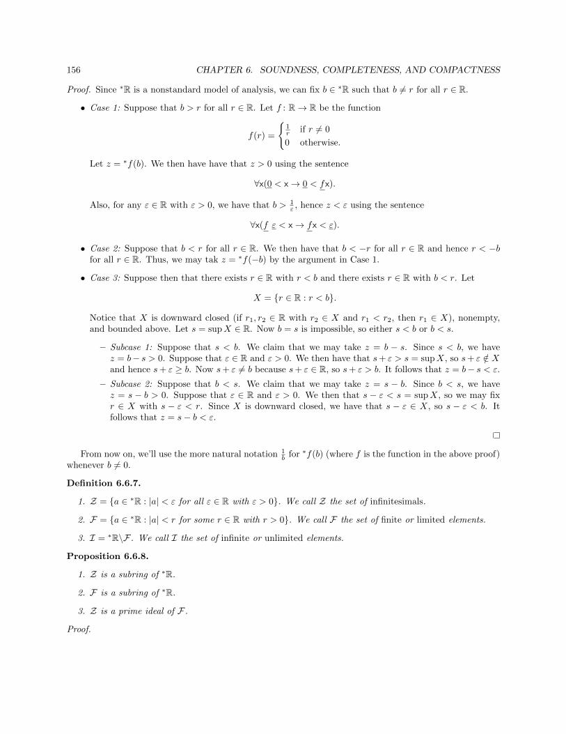
156 CHAPTER 6. SOUNDNESS, COMPLETENESS, AND COMPACTNESS
Proof. Since ∗R is a nonstandard model of analysis, we can fix b ∈ ∗R such that b 6= r for all r ∈ R.
• Case 1: Suppose that b > r for all r ∈ R. Let f : R→ R be the function
f(r) =
{1r if r 6= 0
0 otherwise.
Let z = ∗f(b). We then have have that z > 0 using the sentence
∀x(0 < x→ 0 < fx).
Also, for any ε ∈ R with ε > 0, we have that b > 1ε , hence z < ε using the sentence
∀x(f ε < x→ fx < ε).
• Case 2: Suppose that b < r for all r ∈ R. We then have that b < −r for all r ∈ R and hence r < −bfor all r ∈ R. Thus, we may tak z = ∗f(−b) by the argument in Case 1.
• Case 3: Suppose then that there exists r ∈ R with r < b and there exists r ∈ R with b < r. Let
X = {r ∈ R : r < b}.
Notice that X is downward closed (if r1, r2 ∈ R with r2 ∈ X and r1 < r2, then r1 ∈ X), nonempty,and bounded above. Let s = supX ∈ R. Now b = s is impossible, so either s < b or b < s.
– Subcase 1: Suppose that s < b. We claim that we may take z = b − s. Since s < b, we havez = b− s > 0. Suppose that ε ∈ R and ε > 0. We then have that s+ ε > s = supX, so s+ ε /∈ Xand hence s+ ε ≥ b. Now s+ ε 6= b because s+ ε ∈ R, so s+ ε > b. It follows that z = b− s < ε.
– Subcase 2: Suppose that b < s. We claim that we may take z = s − b. Since b < s, we havez = s − b > 0. Suppose that ε ∈ R and ε > 0. We then that s − ε < s = supX, so we may fixr ∈ X with s − ε < r. Since X is downward closed, we have that s − ε ∈ X, so s − ε < b. Itfollows that z = s− b < ε.
From now on, we’ll use the more natural notation 1b for ∗f(b) (where f is the function in the above proof)
whenever b 6= 0.
Definition 6.6.7.
1. Z = {a ∈ ∗R : |a| < ε for all ε ∈ R with ε > 0}. We call Z the set of infinitesimals.
2. F = {a ∈ ∗R : |a| < r for some r ∈ R with r > 0}. We call F the set of finite or limited elements.
3. I = ∗R\F . We call I the set of infinite or unlimited elements.
Proposition 6.6.8.
1. Z is a subring of ∗R.
2. F is a subring of ∗R.
3. Z is a prime ideal of F .
Proof.

6.6. NONSTANDARD MODELS OF ANALYSIS 157
1. First notice that Z 6= ∅ because 0 ∈ Z (or we can use Proposition 6.6.6). Let a, b ∈ Z be arbitrary.Let ε ∈ R with ε > 0. We have that ε
2 ∈ R and ε2 > 0, hence |a| < ε
2 and |b| < ε2 . It follows that
|a+ b| ≤ |a|+ |b|
<ε
2+ε
2= ε.
Therefore, a+ b ∈ Z. We also have that |a| < 1 and |b| < ε, hence
|a · b| = |a| · |b|< 1 · ε= ε.
Therefore, a · b ∈ Z. Finally, Z is clearly closed under negation.
2. Clearly, F 6= ∅. Let a, b ∈ F be arbitrary. Fix r1, r2 ∈ R with r1, r2 > 0 such that |a| < r1 and |b| < r2.We have
|a+ b| ≤ |a|+ |b|< r1 + r2,
so a− b ∈ F . We also have
|a · b| = |a| · |b|< r1 · r2
so a · b ∈ F . Finally, F is clearly closed under negation.
3. We first show that Z is an ideal of F . We already know from part (1) that Z is closed under additionand negation. Let a ∈ F and b ∈ Z be arbitrary. Fix r ∈ R with r > 0 and |a| < r. Let ε ∈ R withε > 0. We then have that ε
r ∈ R and εr > 0, hence |a| < ε
r . It follows that
|a · b| = |a| · |b|
<ε
r· r
= ε.
Therefore, a · b ∈ Z. It follows that Z is an ideal of F .
We now show that Z is a prime ideal of F . Let a, b ∈ F\Z be arbitrary. We show that a · b /∈ Z. Fixε, δ ∈ R with ε, δ > 0 such that |a| > ε and |b| > δ. We then have |a · b| = |a| · |b| > ε · δ, hence a · b /∈ Z.
Definition 6.6.9. Let a, b ∈ ∗R.
1. We write a ≈ b to mean that a− b ∈ Z.
2. We write a ∼ b to mean that a− b ∈ F .
Proposition 6.6.10. ≈ and ∼ are equivalence relations on ∗R.
Proof. Exercise using Proposition 6.6.8.
158 CHAPTER 6. SOUNDNESS, COMPLETENESS, AND COMPACTNESS
Definition 6.6.11. Let a ∈ ∗R. The ≈-equivalence class of a is called the halo of a. The ∼-equivalenceclass of a is called the galaxy of a.
Proposition 6.6.12. Let a1, b1, a2, b2 ∈ ∗R with a1 ≈ b1 and a2 ≈ b2. We have the following:
1. a1 + a2 ≈ b1 + b2.
2. a1 − a2 ≈ b1 − b2.
3. If a1, b1, a2, b2 ∈ F , then a1 · a2 ≈ b1 · b2.
4. If a1, b1 ∈ F and a2, b2 ∈ F\Z, then a1a2≈ b1
b2.
Proof.
1. We have a1 − b1 ∈ Z and a2 − b2 ∈ Z, hence
(a1 + a2)− (b1 + b2) = (a1 − b1) + (a2 − b2)
is in Z by Proposition 6.6.8.
2. We have a1 − b1 ∈ Z and a2 − b2 ∈ Z, hence
(a1 − a2)− (b1 − b2) = (a1 − b1)− (a2 − b2)
is in Z by Proposition 6.6.8.
3. We have a1 − b1 ∈ Z and a2 − b2 ∈ Z. Notice that
a1 · a2 − b1 · b2 = a1 · a2 − a1 · b2 + a1 · b2 − b1 · b2= a1 · (a2 − b2) + b2 · (a1 − b1).
Since a1 ∈ F and a2−b2 ∈ Z, we may use Proposition 6.6.8 to conclude that a1 ·(a2−b2) ∈ Z. Similarly,we have b2 · (a1 − b1) ∈ Z. Applying Proposition 6.6.8 again, we conclude that a1 · a2 − b1 · b2 ∈ Z.
4. We have a1 − b1 ∈ Z and a2 − b2 ∈ Z. Now
a1
a2− b1b2
=a1 · b2 − a2 · b1
a2 · b2
=1
a2 · b2· (a1 · b2 − a2 · b1),
and we know by part (3) that a1 · b2 − a2 · b1 ∈ Z. Since a2, b2 ∈ F\Z, it follows from Proposition6.6.8 that a2 · b2 ∈ F\Z. Therefore, 1
a2·b2 ∈ F (if ε > 0 is such that |a2 · b2| > ε, then | 1a2·b2 | <
1ε ), so
a1a2− b1
b2∈ Z by Proposition 6.6.8.
Proposition 6.6.13. For every a ∈ F , there exists a unique r ∈ R such that a ≈ r.
Proof. Fix a ∈ F . We first prove existence. Let
X = {r ∈ R : r < a}
and notice that X is downward closed, nonempty, and bounded above because a ∈ F . Now let s = supXand argue as in Case 3 of Proposition 6.6.6 that a ≈ s.
Suppose now that r1, r2 ∈ R are such that a ≈ r1 and a ≈ r2. We then have that r1 ≈ r2 because ≈ is
an equivalence relation. However, this is a contradiction because |r1 − r2| > |r1−r2|2 ∈ R.

6.6. NONSTANDARD MODELS OF ANALYSIS 159
Definition 6.6.14. We define a map st : F → R by letting st(a) be the unique r ∈ R such that a ≈ r. Wecall st(a) the standard part, or shadow, of a.
Corollary 6.6.15. The function st : F → R is a surjective ring homomorphism and ker(st) = Z.
Proposition 6.6.16. Suppose that f : R→ R, and that r, ` ∈ R. The following are equivalent:
1. limx→r
f(x) = `.
2. For all a ≈ r with a 6= r, we have ∗f(a) ≈ `.
Proof. Suppose first that limx→r
f(x) = `. Let a ∈ ∗R\{r} be arbitrary with a ≈ r. Let ε ∈ R with ε > 0.
Since limx→r
f(x) = `, we may fix δ ∈ R with δ > 0 such that |f(x)− `| < ε whenever 0 < |x− r| < δ. Notice
that the sentence
∀x((0 < |x− r| ∧ |x− r| < δ)→ |f(x)− `| < ε)
is in Th(R) = Th(∗R). Now we have a ∈ ∗R and 0 < |a− r| < δ, so |∗f(a)− `| < ε. Since ε was an arbitrarypositive element of R, it follows that ∗f(a)− ` ∈ Z, hence ∗f(a) ≈ `.
Suppose conversely that for all a ≈ r with a 6= r, we have ∗f(a) ≈ `. Fix z ∈ Z with z > 0. Let ε ∈ Rwith ε > 0. By assumption, whenever a ∈ ∗R and 0 < |a − r| < z, we have that ∗f(a) − ` ∈ Z. Thus, thesentence
∃δ(δ > 0 ∧ ∀x((0 < |x− r| ∧ |x− r| < δ)→ |f(x)− `| < ε))
is in Th(∗R) = Th(R). By fixing a witnessing δ, we see that the limit condition holds for ε.
Proposition 6.6.17. Suppose that f, g : R → R, and that r, `,m ∈ R. Suppose also that limx→r
f(x) = ` and
limx→r
g(x) = m. We then have the following:
1. limx→r
(f + g)(x) = `+m.
2. limx→r
(f − g)(x) = `+m.
3. limx→r
(f · g)(x) = ` ·m.
4. If m 6= 0, then limx→r
( fg )(x) = `m .
Proof. In each case, we use Proposition 6.6.16. Let a ≈ r be arbitrary with a 6= r. By assumption andProposition 6.6.16, we then have ∗f(a) ≈ ` and ∗g(a) ≈ m.
1. Notice that the sentence
∀x((f + g)x = fx + gx)
is in Th(∗R) = Th(R). Therefore, we have
∗(f + g)(a) = ∗f(a) + ∗g(a)
≈ `+m (by Proposition 6.6.12).
Using Proposition 6.6.16 again, we conclude that limx→r
(f + g)(x) = `+m.
2. Completely analogous to (1).

160 CHAPTER 6. SOUNDNESS, COMPLETENESS, AND COMPACTNESS
3. As in part (1), we have ∗(f · g)(a) = ∗f(a) · ∗g(a). Therefore,
∗(f + g)(a) = ∗f(a) · ∗g(a)
≈ ` ·m (by Proposition 6.6.12)
where we are using the fact that `,m, ∗f(a), ∗g(a) ∈ F , the latter two of which follow from the factthat they are infinitely close to the former two. Using Proposition 6.6.16 again, we conclude thatlimx→r
(f · g)(x) = ` ·m.
4. Notice that ∗f(a) ∈ F because ∗f(a) ≈ ` ∈ R, and ∗g(a) ∈ F because ∗g(a) ≈ m. We also have∗g(a) /∈ Z because m 6= 0. Therefore,
∗(f
g)(a) =
∗f(a)∗g(a)
≈ `
m(by Proposition 6.6.12).
Using Proposition 6.6.16 again, we conclude that limx→r
( fg )(x) = `m .
Since continuity and differentiability can be defined in terms of limits, we immediately obtain the followingtwo facts.
Corollary 6.6.18. Suppose that f : R→ R, and that r ∈ R. The following are equivalent:
1. f is continuous at r.
2. For all a ≈ r, we have ∗f(a) ≈ f(r).
Corollary 6.6.19. Suppose that f : R→ R and that r, ` ∈ R. The following are equivalent:
1. f is differentiable at r with f ′(r) = `.
2. For all a ≈ r with a 6= r, we have∗f(a)−f(r)
a−r ≈ `.
Proposition 6.6.20. If f is differentiable at r, then f is continuous at r.
Proof. Let a ≈ r be arbitrary with a 6= r. Since f is differentiable at r, we have
∗f(a)− f(r)
a− r≈ f ′(r).
Now f ′(r) ∈ F trivially, so∗f(a)−f(r)
a−r ∈ F . Furthermore, we have a− r ∈ Z, so
∗f(a)− f(r) =∗f(a)− f(r)
a− r· (a− r) ∈ Z
by Proposition 6.6.8. It follows that ∗f(a) ≈ f(r).

Chapter 7
Introduction to Axiomatic Set Theory
No one shall expel us from the paradise that Cantor has created. - David Hilbert
7.1 Why Set Theory?
Set theory originated in an attempt to understand and somehow classify “small” or “negligible” sets ofreal numbers. Cantor’s early explorations in the realm of the transfinite were motivated by a desire tounderstand the points of convergence of trigonometric series. The basic ideas quickly became a fundamentalpart of analysis.
Since then, set theory has become a way to unify mathematical practice, and the way in which math-ematicians deal with the infinite in all areas of mathematics. We’ve all seen the proof that the set of realnumbers is uncountable, but what more can be said? Exactly how uncountable is the set of real numbers?Does this taming of the infinite give us any new tools to prove interesting mathematical theorems? Is thereanything more that the set-theoretic perspective provides to the mathematical toolkit other than a crudenotion of size and cute diagonal arguments?
We begin by listing a few basic questions from various areas of mathematics that can only be tackledwith a well-defined theory of the infinite which set theory provides.
Algebra: A fundamental result in linear algebra is that every finitely generated vector space has a basis,and any two bases have the same size. We call the unique size of any basis of a vector space the dimensionof that space. Moreover, given two finitely generated vectors spaces, they are isomorphic precisely whenthey have the same dimension. What can be said about vector spaces that aren’t finitely generated? Doesevery vector space have a basis? Is there a meaningful way to assign a “dimension” to every vector spacein such a way that two vector spaces over the same field are isomorphic if and only if they have the same“dimension”? We need a well-defined and robust notion of infinite sets and infinite cardinality to deal withthese questions.
Analysis: Lebesgue’s theory of measure and integration require an important distinction between count-able and uncountable sets. Aside from this use, the study of the basic structure of the Borel sets or theprojective sets (an extension of the Borel sets) require some sophisticated use of set theory, in a way thatcan be made precise.
Foundations: A remarkable side-effect of our undertaking to systematically formalize the infinite is thatwe can devise a formal axiomatic and finitistic system in which virtually all of mathematical practice canbe embedded in an extremely faithful manner. Whether this fact is interesting or useful depends on yourphilosophical stance about the nature of mathematics, but it does have an important consequence. It puts usin a position to prove that certain statements do not follow from the axioms (which have now been formallydefined and are thus susceptible to a mathematical analysis), and hence can not be proven by the currently
161

162 CHAPTER 7. INTRODUCTION TO AXIOMATIC SET THEORY
accepted axioms. For better or worse, this feature has become the hallmark of set theory. For example, wecan ask questions like:
1. Do we really need the Axiom of Choice to produce a nonmeasurable set of real numbers?
2. Is there an uncountable set of real numbers which can not be in one-to-one correspondence with theset of all real numbers?
Aside from these ideas which are applicable to other areas of mathematics, set theory is a very activearea of mathematics with its own rich and beautiful structure, and deserves study for this reason alone.
7.2 Motivating the Axioms
In every modern mathematical theory (say group theory, topology, the theory of Banach spaces), we startwith a list of axioms, and derive results from these. In most of the fields that we axiomatize in this way,we have several models of the axioms in mind (many different groups, many different topological spaces,etc.), and we’re using the axiomatization to prove abstract results which will be applicable to each of thesemodels. In set theory, we may think that it is our goal to study one unique universe of sets, and so ouroriginal motivation in writing down axioms is simply to state precisely what we are assuming in an area thatcan often be very counterintuitive. Since we will build our system in first-order logic, it turns out that thereare many models of set theory as well (assuming that there is at least one...), and this is the basis for provingindependence results, but this isn’t our initial motivation. This section will be a little informal. We’ll givethe formal axioms (in a formal first-order language) and derive consequences starting in the next section.
Whether the axioms that we are writing down now are “obviously true”, “correct”, “justified”, or evenworthy of study are very interesting philosophical questions, but we will not spend much time on them here.Regardless of their epistemological status, they are now nearly universally accepted as the “right” axioms touse in the development of set theory. The objects of our theory are sets, and we have one binary relation ∈which represents set membership. That is, we write x ∈ y to mean that x is an element of y. We begin withan axiom which ensures that our theory is not vacuous.
Axiom of Existence: There exists a set.
We need to have an axiom which says how equality of sets is determined in terms of the membershiprelation. In mathematical practice using naive set theory, the most common way to show that two sets Aand B are equal is to show that each is a subset of the other. We therefore define A ⊆ B to mean that forall x ∈ A, we have x ∈ B, and we want to be able to conclude that A = B from the facts that A ⊆ B andB ⊆ A. That is, we want to think of a set as being completely determined by its members, thus linking =and ∈, but we need to codify this as an axiom.
Axiom of Extensionality: For any two sets A and B, if A ⊆ B and B ⊆ A, then A = B.
The Axiom of Extensionality implicitly implies a few, perhaps unexpected, consequences about the natureof sets. First, if a is a set, then we should consider the two sets {a} and {a, a} (if we are allowed to asserttheir existence) to be equal because they have the same elements. Similarly, if a and b are sets, then weshould consider {a, b} and {b, a} to be equal. Hence, whatever a set is, it should be inherently unorderedand have no notion of multiplicity. Also, since the only objects we are considering are sets, we are rulingout the existence of “atoms” other than the empty set, i.e. objects a which are not the empty set but whichhave no elements.
We next need some rules about how we are allowed to build sets. The naive idea is that any propertywe write down determines a set. That is, for any property P of sets, we may form the set {x : P (x)}. For

7.2. MOTIVATING THE AXIOMS 163
example, if we have a group G, we may form the center of G given by Z(G) = {x : x ∈ G and xy = yx forall y ∈ G}. Of course, this naive approach leads to the famous contradiction known as Russell’s paradox.Let P (x) be the property x /∈ x, and let z = {x : P (x)} = {x : x /∈ x}. We then have z ∈ z if and only ifz /∈ z, a contradiction.
This gives our first indication that it may be in our best interest to tread carefully when giving rules abouthow to build sets. One now standard reaction to Russell’s Paradox and other similar paradoxes in naive settheory is that the set-theoretic universe is too “large” to encapsulate into one set. Thus, we shouldn’t allowourselves the luxury of forming the set {x : P (x)} because by doing so we may package too much into oneset, and the set-theoretic universe is too “large” to make this permissible. In other words, we should onlychristen something as a set if it is not too “large”.
However, if we already have a set A and a property P , we should be allowed to from {x ∈ A : P (x)}because A is a set (hence not too “large”), so we should be allowed to assert that the subcollection consistingof those sets x in A such that P (x) holds is in fact a set. For example, if we have a group G (so G is alreadyknown to be a set), its center Z(G) is a set because Z(G) = {x ∈ G : xy = yx for all y ∈ G}. Following thisidea, we put forth the following axiom.
Axiom of Separation: For any set A and any property P of sets, we may form the set consisting ofprecisely those x ∈ A such that P (x), i.e. we may form the set {x ∈ A : P (x)}.
You may object to this axiom because of the vague notion of a “property” of sets, and that would certainlybe a good point. We’ll make it precise when we give the formal first-order axioms in the next section. TheAxiom of Separation allows us to form sets from describable subcollections of sets we already know exist,but we currently have no way to build larger sets from smaller ones. We now give axioms which allow us tobuild up sets in a permissible manner.
Our first axiom along these lines will allow us to conclude that for any two sets x and y, we may putthem together into a set {x, y}. Since we already have the Axiom of Separation, we will state the axiom inthe (apparently) weaker form that for any two sets x and y, there is a set with both x and y as elements.
Axiom of Pairing: For any two sets x and y, there is a set A such that x ∈ A and y ∈ A.
We next want to have an axiom which allows us to take unions. However, in mathematics, we oftenwant to take a union over a (possibly infinite) family of sets. For example, we may have a set An foreach natural number n, and then want to consider
⋃n∈NAn. By being clever, we can incorporate all of
these ideas of taking unions into one axiom. The idea is the following. Suppose that we have two setsA and B, say A = {u, v, w} and B = {x, z}. We want to be able to assert the existence of the union ofA and B, which is {u, v, w, x, z}. First, by by the Axiom of Pairing, we may form the set F = {A,B},which equals {{u, v, w}, {x, z}}. Now the union of A and B is the set of elements of elements of F . In theabove example, if we can form the set F = {A1, A2, A3, . . . } (later axioms will justify this), then
⋃n∈NAn
is the set of elements of elements of F . Again, in the presence of the Axiom of Separation, we state thisaxiom in the (apparently) weaker form that for any set F , there is set containing all elements of elements of F .
Axiom of Union: For any set F , there is a set U such that for all sets x, if there exists A ∈ F with x ∈ A,then x ∈ U .
We next put forward two axioms which really allow the set-theoretic universe to expand. The first is thePower Set Axiom which tells us that if we have a set A, it is permissible to form the set consisting of allsubsets of A.
Axiom of Power Set: For any set A, there is a set F such that for all sets B, if B ⊆ A, then B ∈ F .

164 CHAPTER 7. INTRODUCTION TO AXIOMATIC SET THEORY
Starting with the empty set ∅ (which exists using the Axiom of Existence and the Axiom of Separation),we can build a very rich collection of finite sets using the above axioms. For example, we can form {∅} usingthe Axiom of Pairing. We can also form {∅} by applying the Axiom of Power Set to ∅. We can then go onto form {∅, {∅}} and many other finite sets. However, our axioms provide no means to build an infinite set.
Before getting to the Axiom of Infinity, we will lay some groundwork about ordinals. If set theory is goingto serve as a basis for mathematics, we certainly need to be able to embed within it the natural numbers.It seems natural to represent the number n as some set which we think of as having n elements. Which setshould we choose? Let’s start from the bottom-up. The natural choice to play the role of 0 is ∅ because it isthe only set without any elements. Now that we have 0, and we want 1 to be a set with one element, perhapswe should let 1 be the set {0} = {∅}. Next, a canonical choice for a set with two elements is {0, 1}, so we let2 = {0, 1} = {∅, {∅}}. In general, if we have defined 0, 1, 2, . . . , n, we can let n+ 1 = {0, 1, . . . , n}. This wayof defining the natural numbers has many advantages which we’ll come to appreciate. For instance, we’llhave n < m if and only if n ∈ m, so we may use the membership relation to define the standard ordering ofthe natural numbers.
However, the . . . in the above definition of n+ 1 may make you a little nervous. Fortunately, we can giveanother description of n + 1 which avoids this unpleasantness. If we’ve defined n, we let n + 1 = n ∪ {n},which we can justify the existence of using the Axiom of Pairing and the Axiom of Union. The elements ofn + 1 will then be n, and the elements of n which should “inductively” be the natural numbers up to, butnot including, n.
Using the above outline, we can use our axioms to justify the existence of any particular natural numbern (or, more precisely, the set that we’ve chosen to represent our idea of the natural number n). However,we can’t justify the existence of the set of natural numbers {0, 1, 2, 3, . . . }. To enable us to do this, we makethe following definition. For any set x, let S(x) = x ∪ {x}. We call S(x) the successor of x. We want anaxiom which says that there is a set containing 0 = ∅ which is closed under successors.
Axiom of Infinity: There exists a set A such that ∅ ∈ A and for all x, if x ∈ A, then S(x) ∈ A.
With the Axiom of Infinity asserting existence, it’s not too difficult to use the above axioms to showthat there is a smallest (with respect to ⊆) set A such that ∅ ∈ A and for all x, if x ∈ A, then S(x) ∈ A.Intuitively, this set is the collection of all natural numbers. Following standard set-theoretic practice, wedenote this set by ω (this strange choice, as opposed to the typical N, conforms with the standard practiceof using lowercase greek letters to represent infinite ordinals).
With the set of natural numbers ω in hand, there’s no reason to be timid and stop counting. We startedwith 0, 1, 2, . . . , where each new number consisted of collecting the previous numbers into a set, and we’venow collected all natural numbers into a set ω. Why not continue the counting process by consideringS(ω) = ω ∪ {ω} = {0, 1, 2, . . . , ω}? We call this set ω + 1 for obvious reasons. This conceptual leap ofcounting into the so-called transfinite gives rise to the ordinals, the “numbers” which form the backbone ofset theory.
Once we have ω+ 1, we can then form the set ω+ 2 = S(ω+ 1) = {0, 1, 2, . . . , ω, ω+ 1}, and continue onto ω + 3, ω + 4, and so on. Why stop there? If we were able to collect all of the natural numbers into a set,what’s preventing us from collecting these into the set {0, 1, 2, . . . , ω, ω+1, ω+2, . . . }, and continuing? Well,our current axioms are preventing us, but we shouldn’t let that stand in our way. If we can form ω, surelywe should have an axiom allowing us to make this new collection a set. After all, if ω isn’t too “large”, thisset shouldn’t be too “large” either since it’s just another sequence of ω many sets after ω.
The same difficulty arises when you want to take the union of an infinite family of sets. In fact, theprevious problem is a special case of this one, but in this generality it may feel closer to home. Suppose wehave sets A0, A1, A2, . . . , that is, we have a set An for every n ∈ ω. Of course, we should be able to justifymaking the union
⋃n∈ω An into a set. If we want to apply the Axiom of Union, we should first form the
7.2. MOTIVATING THE AXIOMS 165
set F = {A0, A1, A2, . . . } and apply the axiom to F . However, in general, our current axioms don’t justifyforming this set despite its similarity to asserting the existence of ω.
To remedy these defects, we need a new axiom. In light of the above examples, we want to say somethingalong the lines of “if we can index a family of sets with ω, then we can form this family into a set”. Using thisprinciple, we should be able to form the set {ω, ω + 1, ω + 2, . . . } and hence {0, 1, 2, . . . , ω, ω + 1, ω + 2, . . . }is a set by the Axiom of Union. Similarly, in the second example, we should be able to form the set{A0, A1, A2, . . . }. In terms of our restriction of not allowing sets to be too “large”, this seems justifiedbecause if we consider ω to not be too “large”, then any family of sets it indexes shouldn’t be too “large”either.
There is no reason to limit our focus to ω. If we have any set A, and we can index a family of sets usingA, then we should be able to assert the existence of a set containing the elements of the family. We alsowant to make the notion of indexing more precise, and we will do it using the currently vague notion of aproperty of sets as used in the Axiom of Separation.
Axiom of Collection: Suppose that A is a set and P (x, y) is a property of sets such that for every x ∈ A,there is a unique set y such that P (x, y) holds. Then there is a set B such that for every x ∈ A, we havey ∈ B for the unique y such that P (x, y) holds.
Our next axiom is often viewed as the most controversial due to its nonconstructive nature and thesometimes counterintuitive results it allows us to prove. I will list it here as a fundamental axiom, but wewill avoid using it in the basic development of set theory below until we get to a position to see it’s usefulnessin mathematical practice.
The Axiom of Separation and the Axiom of Collection involved the somewhat vague notion of property,but whenever we think of a property (and the way we will make the notion of property precise using aformal language) we have a precise unambiguous definition which describes the property in mind. Our nextaxiom, the Axiom of Choice, asserts the existence of certain sets without the need for such a nice description.Intuitively, it says that if we have a set consisting only of nonempty sets, there is a function which picks anelement out each of these nonempty sets without requiring that there be a “definable” description of sucha function. We haven’t defined the notion of a function in set theory, and it takes a little work to do, sowe will state the axiom in the following form: For every set F of nonempty pairwise disjoint sets, there is aset C consisting of exactly one element from each element of F . We think of C as a set which “chooses” anelement from each of the elements of F . Slightly more precisely, we state the axiom as follows.
Axiom of Choice: Suppose that F is a set such every A ∈ F is nonempty, and for every A,B ∈ F , if thereexists a set x with x ∈ A and x ∈ B, then A = B. There exists a set C such that for every A ∈ F , there isa unique x ∈ C with x ∈ A.
Our final axiom is in no way justified by mathematical practice because it never appears in argumentsoutside set theory. It is also somewhat unique among our axioms in that in asserts that certain types of setsdo not exist. However, adopting it gives a much clearer picture of the set-theoretic universe and it will cometo play an important role in the study of set theory itself. As with the Axiom of Choice, we will avoid usingit in the basic development of set theory below until we are able to see its usefulness to us.
The goal is to eliminate sets which appear circular in terms of the membership relation. For example, wewant to forbid sets x such that x ∈ x (so there is no set x such that x = {x}). Similarly, we want to forbidthe existence of sets x and y such that x ∈ y and y ∈ x. In more general terms, we don’t want to have aset with an infinite descending chain each a member of the next, such as having sets xn for each n ∈ ω suchthat · · · ∈ x2 ∈ x1 ∈ x0. We codify this by saying every nonempty set A has an element which is minimalwith respect to the membership relation.

166 CHAPTER 7. INTRODUCTION TO AXIOMATIC SET THEORY
Axiom of Foundation: If A is a nonempty set, then there exists x ∈ A such that there is no set z withboth z ∈ A and z ∈ x.
7.3 Formal Axiomatic Set Theory
We now give the formal version of our axioms. We work in a first-order language L with a single binaryrelation symbol ∈. By working in this first-order language, we are able to make precise the vague notion ofproperty discussed above by using first-order formulas instead. However, this comes at the cost of replacingthe Axiom of Separation and the Axiom of Collection by infinitely many axioms (also called an axiom scheme)since we can’t quantify over formulas within the theory itself. There are other more subtle consequences offormalizing the above intuitive axioms in first-order logic which we will discuss below.
Notice also that we allow parameters (denoted by ~p) in the Axioms of Separation and Collection so thatwe will be able to derive statements which universally quantified over a parameter, such as “For all groupsG, the set Z(G) = {x ∈ G : xy = yx for all x ∈ G} exists”, rather than having to reprove that Z(G) isa set for each group G that we know exists. Finally, notice how we can avoid using defined notions (like∅, ⊆, and S(x) in the Axiom of Infinity) by expanding them out into our fixed language. For example, wereplace x ⊆ y by ∀w(w ∈ x→ w ∈ y) and replace ∅ ∈ z by ∃w(∀y(y /∈ w) ∧ w ∈ z) (we could also replace it∀w(∀y(y /∈ w)→ w ∈ z)).
In each of the following axioms, when we write a formula ϕ(x1, x2, . . . , xk), we implicitly mean that thexi’s are distinct variables and that every free variable of ϕ is one of the xi. We also use ~p to denote a finitesequence of variables p1, p2, . . . , pk. Notice that we don’t need the Axiom of Existence because it is true inall L-structures (recall that all L-structures are nonempty).
Axiom of Extensionality:∀x∀y(∀w(w ∈ x↔ w ∈ y)→ x = y)
Axiom (Scheme) of Separation: For each formula ϕ(x, y,~p) we have the axiom
∀~p∀y∃z∀x(x ∈ z↔ (x ∈ y∧ϕ(x, y,~p)))
Axiom of Pairing:∀x∀y∃z(x ∈ z ∧ y ∈ z)
Axiom of Union:∀x∃u∀z(∃y(z ∈ y ∧ y ∈ x)→ z ∈ u)
Axiom of Power Set:∀x∃z∀y(∀w(w ∈ y→ w ∈ x)→ y ∈ z)
Axiom of Infinity:
∃z(∃w(∀y(y /∈ w) ∧ w ∈ z) ∧ ∀x(x ∈ z→ ∃y(∀w(w ∈ y↔ (w ∈ x ∨ w = x)) ∧ y ∈ z)))
Axiom (Scheme) of Collection: For each formula ϕ(x, y,~p) we have the axiom
∀~p∀w((∀x(x ∈ w→ ∃yϕ(x, y,~p))∧∀x(x ∈ w→ ∀u∀v((ϕ(x, u,~p) ∧ ϕ(x, v,~p))→ u = v)))
→ ∃z∀x(x ∈ w→ ∃y(y ∈ z ∧ ϕ(x, y,~p))))
Axiom of Choice:
∀z((∀x(x ∈ z→ ∃w(w ∈ x)) ∧ ∀x∀y((x ∈ z ∧ y ∈ z ∧ ∃w(w ∈ x ∧ w ∈ y))→ x = y))
→ ∃c∀x(x ∈ z→ (∃w(w ∈ x ∧ w ∈ c) ∧ ∀u∀v((u ∈ x ∧ v ∈ x ∧ u ∈ c ∧ v ∈ c)→ u = v))))

7.4. WORKING FROM THE AXIOMS 167
Axiom of Foundation:
∀z(∃x(x ∈ z)→ ∃x(x ∈ z ∧ ¬(∃y(y ∈ z ∧ y ∈ x))))
Let AxZFC be the above set of sentences, and let ZFC = Cn(AxZFC) (ZFC stands for Zermelo-Fraenkelset theory with Choice). Other presentations state the axioms of ZFC a little differently, but they allgive the same theory. Some people refer to the Axiom of Separation as the Axiom of Comprehension, butComprehension is sometimes also used to mean the contradictory statement (via Russell’s Paradox) thatwe can always form the set {x : P (x)}, so I prefer to call it Separation. Also, some presentations refer tothe Axiom of Collection as the Axiom of Replacement, but this name is more applicable to the statementthat replaces the last → in the statement of Collection with a ↔, and this formulation implies the Axiom ofSeparation.
7.4 Working from the Axioms
We have set up ZFC as a first-order theory similar to the group axioms, ring axioms, or partial orderingsaxioms. The fact that we have created formal first-order axioms for set theory has several far-reachingand surprising consequences. For example, if ZFC is satisfiable, then since L is countable, there must bea countable model of ZFC. This shocking result may seem to contradict the fact that (as we will see) ZFCproves the existence of uncountable sets. How can these statements not contradict each other? This seemingparadox, known as Skolem’s paradox, can only be understood and resolved once we have a better sense ofwhat models of ZFC look like. Notice also that if ZFC is satisfiable, then there is an uncountable model ofZFC by Proposition 6.3.4. Therefore, if ZFC has a model, then it has several nonisomorphic models. It isvery natural to find all of these facts disorienting, because our original motivation was to write down axiomsfor “the” universe of sets.
What does a model of ZFC look like? Recall that we are working in a language L with just one binaryrelation symbol. An L-structure M in this language can be visualized as a directed graph, where we drawan arrow from vertex u to vertex v if (u, v) is an element of ∈M. Given a vertex v in such a directedgraph, the set of predecessors of v is just the set of vertices that have an arrow pointing to v. From thisperspective, the Axiom of Extensionality says that if two vertices have the same set of predecessors, theythen must be the same vertex. The Axiom of Pairing says that given any two vertices u and w, we canalways find a vertex v such that u and w are both predecessors of u. For a more interesting example, theAxiom of Separation says that given any vertex v, if we consider any subset of the predecessors of v thatis definable (with parameters), then there is a vertex u whose predecessors consist of exactly this definablesubset. Moreover, a defined notion like “u is a subset of w” just means that the set of predecessors of u is asubset of the set of predecessors of w.
For a concrete example, consider the L-structure N = (N, <). As a directed graph, we have a vertex mfor each natural number, and we have an arrow from m to n if and only if m < n. We determine which ofthe ZFC axioms are true in N:
• Axiom of Extensionality: In the structure N, this interprets as saying that whenever two elements ofN have the same elements of N less than them, then they are equal. This holds in N.
• Axiom (Scheme) of Separation: This does not hold in N. Let ϕ(x, y) be the formula ∃w(w ∈ x). Thecorresponding instance of Separation is:
∀y∃z∀x(x ∈ z↔ (x ∈ y ∧ ∃w(w ∈ x)))
In the structure N, this interprets as saying that for all n ∈ N, there is an m ∈ N such that for allk ∈ N, we have k < m if and only if k < n and k 6= 0. This does not hold in N because if we considern = 2, there is no m ∈ N such that 0 6< m and yet 1 < m.

168 CHAPTER 7. INTRODUCTION TO AXIOMATIC SET THEORY
• Axiom of Pairing: In the structure N, this interprets as saying that whenever m,n ∈ N, there existsk ∈ N such that m < k and n < k. This holds in N because given m,n ∈ N, we may take k =max{m,n}+ 1.
• Axiom of Union: In the structure N, this interprets as saying that whenever n ∈ N, there exists ` ∈ Nsuch that whenever k ∈ N has the property that there exists m ∈ N with k < m and m < n, thenk < `. This holds in N because given n ∈ N, we may take ` = n since if k < m and m < n, then k < nby transitivity of < in N (in fact, we may take ` = n− 1 if n 6= 0).
• Axiom of Power Set: In the structure N, this interprets as saying that whenever n ∈ N, there exists` ∈ N such that whenever m ∈ N has the property that every k < m also satisfies k < n, then m < `.This holds in N because given n ∈ N, we may take ` = n + 1 since if m ∈ N has the property thatevery k < m also satisfies k < n, then m ≤ n and hence m < n+ 1.
• Axiom of Infinity: In the structure N, this interprets as saying that there exists n ∈ N such that 0 < nand whenever m < n, we have m+ 1 < n. This does not hold in N.
• Axiom (Scheme) of Collection: This holds in N, as we now check. Fix a formula ϕ(x, y,~p). Interpretingin N, we need to check that if we fix natural numbers ~q and an n ∈ N such that for all k < n thereexists a unique ` ∈ N such that (N, k, `, ~q) � ϕ, then there exists m ∈ N such that for all k < n thereexists an ` < m such that (N, k, `, ~q) � ϕ. Let’s then fix natural numbers ~q and an n ∈ N, and supposethat for all k < n there exists a unique ` ∈ N such that (N, k, `, ~q) � ϕ. For each k < n, let `k bethe unique element of N such that (N, k, `k, ~q) � ϕ. Letting m = max{`k : k < n}+ 1, we see that msuffices. Therefore, this holds in N.
• Axiom of Choice: In the structure N, this interprets as saying that whenever n ∈ N is such that
– Every m < n is nonzero.
– For all `,m < n, there is no k with k < ` and k < m
then there exists m ∈ N such that for all k < n, there is exactly one ` ∈ N with ` < m and ` < n.Notice that the only n ∈ N satisfying the hypothesis (that is, the above two conditions) is n = 0. Nowfor n = 0, the condition is trivial because we may take m = 0 as there is no k < 0. Therefore, thisholds in N.
• Axiom of Foundation: In the structure N, this interprets as saying that whenever n ∈ N has theproperty that there is some m < n, there there exists m < n such that there is no k with k < m andk < n. Notice that n ∈ N has the property that there is some m < n if and only if n 6= 0. Thus, thisholds in N because if n 6= 0, then we have that 0 < n and there is no k with k < 0 and k < n.
Is ZFC, or equivalently AxZFC , satisfiable? Can we somehow construct a model of ZFC? These areinteresting questions with subtle answers. For now, we’ll just have to live with a set of axioms with noobvious models. How then do we show that an L-sentence σ is in ZFC? Since we have two notions ofimplication (semantic and syntactic), we can show that either AxZFC � σ or AxZFC ` σ. Given ourexperience with syntactic deductions, of course we will choose the the former. When attempting to showthat AxZFC � σ, we must take an arbitrary model of AxZFC and show that it is a model of σ. Even thoughwe do not have a simple natural example of such a model, we can still argue in this way, but we must bemindful of strange L-structures and perhaps unexpected models.
Thus, when we develop set theory below, we will be arguing semantically via models. Rather thatconstantly saying “Fix a model M of AxZFC” at the beginning of each proof, and proceeding by showingthat (M, s) � ϕ for various ϕ, we will keep the models in the background and assume that we are “living”inside one for each proof. When we are doing this, a “set” is simply an element of the universe M of

7.5. ZFC AS A FOUNDATION FOR MATHEMATICS 169
our model M, and given two “sets” a and b, we write a ∈ b to mean that (a, b) is an element of ∈M.Notice that this approach is completely analogous to what we do in group theory. That is, when provingthat statement is true in all groups, we take an arbitrary group, and “work inside” that group with theappropriate interpretations of the symbols.
Also, although there is no hierarchy of sets in our axioms, we will often follow the practice of usinglowercase letters a, b, c, etc. to represent sets that we like to think of as having no internal structure (suchas numbers, elements of a group, points of a topological space), use capital letters A,B,C, etc. to representsets whose elements we like to think of as having no internal structure, and use script letters A,F , etc. torepresent sets of such sets. Again, an arbitrary model of ZFC can be viewed as a directed graph, so everyelement of the model is a certain vertex (like any other) in this structure. In other words, our notationalchoices are just for our own human understanding.
7.5 ZFC as a Foundation for Mathematics
In the next few chapters, we’ll show how to develop mathematics quite faithfully within the framework ofZFC. This raises the possibility of using set theory as a foundation for mathematical practice. However, thisseems circular because our development of logic presupposed normal mathematical practice and “naive” settheory (after all, we have the set of axioms of ZFC). It seems that logic depends on set theory and set theorydepends on logic, so how have we gained anything from a foundational perspective?
It is indeed possible, at least in principle, to get out of this vicious circle and have a completely finististicbasis for mathematics. The escape is to buckle down and use syntactic arguments. In other words, we canshow that AxZFC ` σ instead of showing that AxZFC � σ. Now there are infinitely many axioms of ZFC(because of the two axioms schemes), but any given deductions will only use finitely many of the axioms.Furthermore, although there are infinitely many axioms, we can mechanically check if a given L-sentencereally is an axiom. Informally, the set of axioms is a “computable” set. In this way, it would be possible inprinciple to make every proof completely formal and finitistic, where each line follows from previous lines byone of our proof rules. If we held ourselves to this style, then we could reduce mathematical practice to agame with finitely many symbols (if we insisted on avoiding reference to the natural numbers explicity, wecould replace our infinite stock of variables V ar with one variable symbol x, introduce a new symbol ′, andrefer to x3 as x′′′, etc.) where each line could be mechanically checked according to our finitely many rules.Thus, it would even be possible to program a computer to check every proof.
In practice (for human beings at least), the idea of giving deductions for everything is outlandish. Leavingaside the fact that actually giving short deductions is often a painful endeavor, it turns out that even themost basic statements of mathematics, when translated into ZFC, are many thousands of symbols long, andelementary mathematical proofs (such as say the Fundamental Theorem of Arithmetic) are many thousandsof lines long. We’ll discuss how to develop the real numbers below, but any actual formulas talking aboutreal numbers would be ridiculously long and incomprehensible to the human reader. Due to these reasons,and since the prospect of giving syntactic deductions for everything should gives me nightmares, we willargue everything semantically in the style of any other axiomatic subject in mathematics. It is an interestingand worthwhile exercise, however, to imagine how everything could be done syntactically.

170 CHAPTER 7. INTRODUCTION TO AXIOMATIC SET THEORY

Chapter 8
Developing Basic Set Theory
8.1 First Steps
We first establish some basic set theoretic facts carefully from the axioms.
Definition 8.1.1. If A and B are sets, we write A ⊆ B to mean for all c ∈ A, we have c ∈ B.
Although the symbol ⊆ is not part of our language, we will often use ⊆ in our formulas and arguments.This use is justified because it can always be transcribed into our language by replacing it with the corre-sponding formula as we did in the axioms. As mentioned previously, if we have a model M of ZFC viewedas a directed graph, and we also have a, b ∈M , then a ⊆ b will be try in M if every vertex that points to aalso points to b. In other words, always remember that although we call elements “sets”, in any given model,these “sets” can be viewed as vertices of a directed graph with certain properties. From this perspective,the next result says that in any model of ZFC, there is a unique vertex that has no incoming arrows.
Proposition 8.1.2. There is a unique set with no elements.
Proof. Fix a set b (which exists by the Axiom of Existence, or because L-structures are nonempty bydefinition). By Separation applied to the formula x 6= x, there is a set c such that for all a, we have a ∈ c ifand only if a ∈ b and a 6= a. Now for all sets a, we have a = a, hence a /∈ c. Therefore, there is a set with noelements. If c1 and c2 are two sets with no elements, then by the Axiom of Extensionality, we may concludethat c1 = c2.
Definition 8.1.3. We use ∅ to denote the unique set with no elements.
As above, we will often use ∅ in our formulas and arguments despite the fact that there is no constant inour language representing it. Again, this use can always be eliminated by replacing it with a formula, as wedid in the Infinity, Choice, and Foundation axioms. We will continue to follow this practice without commentin the future when we introduce new definitions to stand for sets for which ZFC proves both existence anduniqueness. In each case, be sure to understand how these definitions could be eliminated.
We now show how to turn the idea of Russell’s Paradox into a proof that there is no universal set.
Proposition 8.1.4. There is no set u such that a ∈ u for every set a.
Proof. We prove this by contradiction. Suppose that u is a set with the property that a ∈ u for every set a.By Separation applied to the formula ¬(x = x), there is a set c such that for all sets a, we have a ∈ c if andonly if a ∈ u and a /∈ a. Since a ∈ u for every set a, it follows that for each set a, we have a ∈ c if and onlyif a /∈ a. Therefore, c ∈ c if and only if c /∈ c, a contradiction.
171

172 CHAPTER 8. DEVELOPING BASIC SET THEORY
Proposition 8.1.5. For all sets a and b, there is a unique set c such that, for all sets d, we have d ∈ c ifand only if either d = a or d = b.
Proof. Let a and b be arbitrary sets. By Pairing, there is a set e such that a ∈ e and b ∈ e. By Separationapplied to the formula x = a ∨ x = b (notice that we are using parameters a and b in this use of Separation),there is a set c such that for all d, we have d ∈ c if and only if both d ∈ e and either d = a or d = b. Itfollows that a ∈ c, b ∈ c, and for any d ∈ c, we have either d = a or d = b. Uniqueness again follows fromExtensionality.
Corollary 8.1.6. For every set a, there is a unique set c such that, for all sets d, we have d ∈ c if and onlyif d = a.
Proof. Apply the previous proposition with b = a.
Definition 8.1.7. Given two sets a and b, we use the notation {a, b} to denote the unique set guaranteed toexist by the Proposition 8.1.5. Given a set a, we use the notation {a} to denote the unique set guaranteedto exist by the Corollary 8.1.6.
Using the same style of argument, we can use Union and Separation to show that for every set F , thereis a unique set z consisting precisely of elements of elements of F .
Proposition 8.1.8. Let F be a set. There is a unique set U such that for all a, we have a ∈ U if and onlyif there exists B ∈ F with a ∈ B.
Proof. Exercise.
Definition 8.1.9. Let F be a set. We use the notation⋃F to denote the unique set guaranteed to exist by
the previous proposition. If A and B are sets, we use the notation A ∪B to denote⋃{A,B}.
We now introduce some notation which conforms with the normal mathematical practice of writing sets.
Definition 8.1.10. Suppose that ϕ(x, y,~p) is a formula (in our language L = {∈}), and that B and ~q aresets. By Separation and Extensionality, there is a unique set C such that for all sets a, we have a ∈ C ifand only if a ∈ B and ϕ(a,B, ~q). More formally, given a model M of ZFC and elements B, ~q of M , there isunique element C of M such that for all a, we have a ∈ C if and only if a ∈ M and (M, a, B, ~q) � ϕ. Wedenote this unique set by {a ∈ B : ϕ(a,B, ~q)}.
With unions in hand, what about intersections? As in unions, the general case to consider is when wehave a set F , which we think of as a family of sets. We then want to collect those a such that a ∈ B for allB ∈ F into a set. However, we do need to be a little careful. What happens if F = ∅? It seems that ourdefinition would want to make the the intersection of the sets in F consists of all sets, contrary to Proposition8.1.4. However, this is the only case which gives difficulty, because if F 6= ∅, we can take the intersection tobe a subset of one (any) of the elements of F .
Proposition 8.1.11. Let F be a set with F 6= ∅. There is a unique set I such that for all a, we have a ∈ Iif and only if a ∈ B for all B ∈ F .
Proof. Since F 6= ∅, we may fix C ∈ F . Let I = {a ∈ C : ∀B(B ∈ F → a ∈ B)}. For all a, we have a ∈ I ifand only if a ∈ B for all B ∈ F . Uniqueness again follows from Extensionality.
Definition 8.1.12. Let F be a set with F 6= ∅. We use the notation⋂F to denote the unique set guaranteed
to exist by the previous proposition. If A and B are sets, we use the notation A ∩B to denote⋂{A,B}.
If A is a set, then we can not expect the complement of A to be a set because the union of such a purportedset with A would be a set which has every set as an element, contrary to Proposition 8.1.4. However, if Aand B are sets, and A ⊆ B, we can take the relative complement of A in B.
8.1. FIRST STEPS 173
Proposition 8.1.13. Let A and B be sets with A ⊆ B. There is a unique set C such that for all a, we havea ∈ C if and only if a ∈ B and a /∈ A.
Proof. Exercise.
Definition 8.1.14. Let A and B be sets with A ⊆ B. We use the notation B\A, or B − A, to denote theunique set guaranteed to exist by the previous proposition.
Since sets have no internal order to them, we need a way to represent ordered pairs. Fortunately (sinceit means we don’t have to extend our notion of set), there is a hack that allows us to build sets capturingthe only essential property of an ordered pair.
Definition 8.1.15. Given two sets a and b, we let (a, b) = {{a}, {a, b}}.
Proposition 8.1.16. Let a, b, c, d be sets. If (a, b) = (c, d), then a = c and b = d.
Proof. Let a, b, c, d be arbitrary sets with {{a}, {a, b}} = {{c}, {c, d}}. We first show that a = c. Since{c} ∈ {{a}, {a, b}}, either {c} = {a} or {c} = {a, b}. In either case, we have a ∈ {c}, hence a = c. Wenow need only show that b = d. Suppose instead that b 6= d. Since {a, b} ∈ {{c}, {c, d}}, we have either{a, b} = {c} or {a, b} = {c, d}. In either case, we conclude that b = c (because either b ∈ {c}, or b ∈ {c, d}and b 6= d). Similarly, since {c, d} ∈ {{a}, {a, b}}, we have either {c, d} = {a} or {c, d} = {a, b}, and ineither case we conclude that d = a. Therefore, using the fact that a = c, it follows that b = d.
We next turn to Cartesian products. Given two sets A and B, we would like to form the set {(a, b) : a ∈ Aand b ∈ B}. Justifying that we can collect these elements into a set takes a little work, since we don’t have aset that we are “carving” out from. The idea is as follows. For each fixed a ∈ A, we can assert the existenceof {a} × B = {(a, b) : b ∈ B} using Collection (and Separation) because B is a set. Then using Collection(and Separation) again, we can assert the existence of {{a} × B : a ∈ A} since A is a set. The Cartesianproduct is then the union of this set. At later points, we will consider this argument sufficient, but we give aslightly more formal version here to really see how the axioms of Collection and Separation are applied andwhere the formulas come into play.
Proposition 8.1.17. For any two sets A and B, there exists a unique set, denoted by A×B, such that forall x, we have x ∈ A×B if and only if there exists a ∈ A and b ∈ B with x = (a, b).
Proof. Let ϕ(x, a, b) be a formula expressing that “x = (a, b)” (think about how to write this down). Letting∃! be shorthand for “there is a unique”, the following sentence follows (either semantically or syntactically)from AxZFC , and hence is an element of ZFC:
∀a∀B(∀b(b ∈ B→ ∃!xϕ(x, a, b))).
Therefore, by Collection, we may conclude that the following sentence is an element of ZFC:
∀a∀B∃C∀b(b ∈ B→ ∃x(x ∈ C ∧ ϕ(x, a, b))).
Next using Separation and Extensionality, we have the following:
∀a∀B∃!C∀b(b ∈ B↔ ∃x(x ∈ C ∧ ϕ(x, a, b))).
From here, it follows that
∀A∀B∀a(a ∈ A→ ∃!C∀b(b ∈ B↔ ∃x(x ∈ C ∧ ϕ(x, a, b)))).
Using Collection again, we may conclude that
∀A∀B∃F∀a(a ∈ A→ ∃C(C ∈ F ∧ ∀b(b ∈ B↔ ∃x(x ∈ C ∧ ϕ(x, a, b))))),

174 CHAPTER 8. DEVELOPING BASIC SET THEORY
and hence the following is an element of ZFC:
∀A∀B∃F∀a∀b((a ∈ A ∧ b ∈ B)→ ∃C(C ∈ F ∧ ∃x(x ∈ C ∧ ϕ(x, a, b)))).
Now let A and B be arbitrary sets. From the last line above, we may conclude that there exists F such thatfor all a ∈ A and all b ∈ B, there exists C ∈ F with (a, b) ∈ C. Let D =
⋃F . Given any a ∈ A and b ∈ B, we
then have (a, b) ∈ D. Now applying Separation to the set D and the formula ∃a∃b(a ∈ A ∧ b ∈ B ∧ ϕ(x, a, b)),there is a set E such that for all x, we have x ∈ E if and only if there exists a ∈ A and b ∈ B with x = (a, b).As usual, Extensionality gives uniqueness.
Now that we have ordered pairs and Cartesian products, we can really make some progress.
Definition 8.1.18. A relation is a set R such that every set x ∈ R is an ordered pair, i.e. if for every x ∈ R,there exists sets a, b such that x = (a, b).
Given a relation R, we want to define its domain to be the set of first elements of ordered pairs which areelements of R, and we want to define its range to be the set of second elements of ordered pairs which areelements of R. These are good descriptions which can easily (though not shortly) be turned into formulas,but we need to know that there is some set which contains all of these elements in order to apply Separation.Since the elements of an ordered pair (a, b) = {{a}, {a, b}} are “two deep”, a good exercise is to convinceyourself that
⋃⋃R will work. This justifies the following definitions.
Definition 8.1.19. Let R be a relation
1. domain(R) is the set of a such that there exists b with (a, b) ∈ R.
2. range(R) is the set of b such that there exists a with (a, b) ∈ R.
We can define the composition of two relations, generalizing the idea of a composition of functions (wetalk about this special case below).
Definition 8.1.20. Let R and S be relations. Let A = domain(R) and C = range(S). We define
S ◦R = {(a, c) ∈ A× C : There exists b with (a, b) ∈ R and (b, c) ∈ S}.
Definition 8.1.21. Let R be a relation. We write aRb if (a, b) ∈ R.
Definition 8.1.22. Let A be a set. We say that R is a relation on A if domain(R) ⊆ A and range(R) ⊆ A.
We define functions in the obvious way.
Definition 8.1.23. A function f is a relation which is such that for all a ∈ domain(f), there exists a uniqueb ∈ range(f) such that (a, b) ∈ f .
Definition 8.1.24. Let f be a function. We write f(a) = b if (a, b) ∈ f .
The definition of function composition is now a special case of the definition of the composition ofrelations. We do need the following result.
Proposition 8.1.25. If f and g are both functions, then g◦f is a function with domain(g◦f) ⊆ domain(f).
Definition 8.1.26. Let f be a function. f is injective (or an injection) if whenever f(a1) = b and f(a2) = b,we have a1 = a2.
Definition 8.1.27. Let A and B be sets. We write f : A→ B to mean that f is a function, domain(f) = Aand range(f) ⊆ B.

8.1. FIRST STEPS 175
We are now in a position to define when a function f is surjective and bijective. Notice that surjectivityand bijectivity are not properties of a function itself because these notions depend on a set which you considerto contain range(f). Once we have a fixed such set in mind, however, we can make the definitions.
Definition 8.1.28. Let A and B be sets, and let f : A→ B.
1. f is surjective (or a surjection) if range(f) = B.
2. f is bijective (or a bijection) if f is injective and surjective.
Definition 8.1.29. Let A and B be sets.
1. We write A � B to mean that there is an injection f : A→ B.
2. We write A ≈ B to mean that there is a bijection f : A→ B.
Proposition 8.1.30. Let A, B, and C be sets. If A � B and B � C, then A � C.
Proof. Use the fact that the composition of injective functions is injective.
Proposition 8.1.31. Let A, B, and C be sets.
1. A ≈ A.
2. If A ≈ B, then B ≈ A.
3. If A ≈ B and B ≈ C, then A ≈ C.
Definition 8.1.32. Let R be a relation on a set A.
1. R is reflexive on A if for all a ∈ A, we have aRa.
2. R is symmetric on A if for all a, b ∈ A, if aRb then bRa.
3. R is asymmetric on A if for all a, b ∈ A, if aRb then it is not the case that bRa.
4. R is antisymmetric on A if for all a, b ∈ A, if aRb and bRa, then a = b.
5. R is transitive on A if for all a, b, c ∈ A, if aRb and bRc, then aRc.
6. R is connected on A if for all a, b ∈ A, either aRb, a = b, or bRa.
Definition 8.1.33. Let R be a relation on a set A.
1. R is a (strict) partial ordering on A if R is transitive on A and asymmetric on A.
2. R is a (strict) linear ordering on A if R is a partial ordering on A and R is connected on A.
3. R is a (strict) well-ordering on A if R is a linear ordering on A and for every X ⊆ A with X 6= ∅,there exists m ∈ X such that for all x ∈ X, either m = x or mRx.

176 CHAPTER 8. DEVELOPING BASIC SET THEORY
8.2 The Natural Numbers and Induction
We specifically added the Axiom of Infinity with the hope that it captured the idea of the set of naturalnumbers. We now show how this axiom, in league with the others, allows us to embed the theory of thenatural numbers into set theory. We start by defining the initial natural number and successors of sets.
Definition 8.2.1. 0 = ∅
Definition 8.2.2. Given a set x, we let S(x) = x ∪ {x}, and we call S(x) the successor of x.
With 0 and the notion of successor, we can then go on to define 1 = S(0), 2 = S(1) = S(S(0)), andcontinue in this way to define any particular natural number. However, we want to form the set of all naturalnumbers.
Definition 8.2.3. A set I is inductive if 0 ∈ I and for all x ∈ I, we have S(x) ∈ I.
The Axiom of Infinity simply asserts the existence of some inductive set J . Intuitively, we have 0 ∈ J ,S(0) ∈ J , S(S(0)) ∈ J , and so on. However, J may very well contain more than just repeated applicationsof S to 0. We now use the top-down approach of generation to define the natural numbers (the other twoapproaches will not work yet because their very definitions rely on the natural numbers).
Proposition 8.2.4. There is a smallest inductive set. That is, there is an inductive set K such that K ⊆ Ifor every inductive set I.
Proof. By the Axiom of Infinity, we may fix an inductive set J . Let K = {x ∈ J : x ∈ I for every inductiveset I}. Notice that 0 ∈ K because 0 ∈ I for every inductive set I (and so, in particular, 0 ∈ J). Supposethat x ∈ K. If I is inductive, then x ∈ I, hence S(x) ∈ I. It follows that S(x) ∈ I for every inductive set I(and so, in particular, S(x) ∈ J), hence S(x) ∈ K. Therefore, K is inductive. By definition of K, we haveK ⊆ I whenever I is inductive.
By Extensionality, there is a unique smallest inductive set, so this justifies the following definition.
Definition 8.2.5. We denote the unique smallest inductive set by ω.
We think that ω captures our intuitive idea of the set of natural numbers, and it is now our goal to showhow to prove the basic statements about the natural numbers which are often accepted axiomatically. Wefirst define a relation < on ω. Remember our intuitive idea is that ∈ captures the order relationship on thenatural numbers.
Definition 8.2.6.
1. We define a relation < on ω by setting < = {(n,m) ∈ ω × ω : n ∈ m}.
2. We define a relation ≤ on ω by setting ≤ = {(n,m) ∈ ω × ω : n < m or n = m}.
3. We define a relation > on ω by setting > = {(n,m) ∈ ω × ω : m < n}.
4. We define a relation ≥ on ω by setting ≥ = {(n,m) ∈ ω × ω : n > m or n = m}.
Lemma 8.2.7. There is no n ∈ ω with n < 0.
Proof. Since 0 = ∅, there is no set x such that x ∈ 0. Therefore, there is no n ∈ ω with n < 0.
Lemma 8.2.8. Let m,n ∈ ω be arbitrary. We have m < S(n) if and only if m ≤ n.

8.2. THE NATURAL NUMBERS AND INDUCTION 177
Proof. Let m,n ∈ ω. We then have S(n) ∈ ω since ω is inductive, and
m < S(n)⇔ m ∈ S(n)
⇔ m ∈ n ∪ {n}⇔ Either m ∈ n or m ∈ {n}⇔ Either m < n or m = n
⇔ m ≤ n.
This proves the lemma.
Our primary objective is to show that < is a well-ordering on ω. Due to the nature of the definition ofω, it seems that only way to prove nontrivial results about ω is “by induction”. We state the Step InductionPrinciple in two forms. The first is much cleaner and seemingly more powerful (because it immediatelyimplies the second and we can quantify over sets but not over formulas), but the second is how one oftenthinks about induction in practice by using “properties” of natural numbers, and will be the only form thatwe can generalize to the collection of all ordinals.
Proposition 8.2.9 (Step Induction Principle on ω).
1. Suppose that X is a set, 0 ∈ X, and for all n ∈ ω, if n ∈ X then S(n) ∈ X. We then have ω ⊆ X.
2. For any formula ϕ(n,~p), the sentence
∀~p((ϕ(0,~p) ∧ (∀n ∈ ω)(ϕ(n,~p)→ ϕ(S(n),~p)))→ (∀n ∈ ω)ϕ(n,~p))
is in ZFC, where ϕ(0,~p) is shorthand for the formula
∃x(∀y(¬(y ∈ x)) ∧ ϕ(x,~p)),
and ϕ(S(n),~p) is shorthand for the formula
∃x(∀y(y ∈ x↔ (y ∈ n ∨ y = n)) ∧ ϕ(x,~p)).
Proof.
1. Let Y = X ∩ ω. Notice first that 0 ∈ Y . Suppose now that n ∈ Y = X ∩ ω. We then have n ∈ ωand n ∈ X, so S(n) ∈ ω (because ω is inductive), and S(n) ∈ X by assumption. Hence, S(n) ∈ Y .Therefore, Y is inductive, so we may conclude that ω ⊆ Y . It follows that ω ⊆ X.
2. Let ~q be an arbitrary sequence of sets, and suppose ϕ(0, ~q) and (∀n ∈ ω)(ϕ(n, ~q) → ϕ(S(n), ~q)). LetX = {n ∈ ω : ϕ(n, ~q)}, which exists by Separation. Notice that 0 ∈ X and for all n ∈ ω, if n ∈ X thenS(n) ∈ X by assumption. It follows from part 1 that ω ⊆ X. Therefore, we have (∀n ∈ ω)ϕ(n, ~q).
With the Step Induction Principle in hand, we can begin to prove the basic facts about the naturalnumbers. Our goal is to prove that < is a well-ordering on ω, but it will take some time to get there.We first give a very simple inductive proof. For this proof only, we will give careful arguments using bothversions of Step Induction to show how a usual induction proof can be formalized in either way.
Lemma 8.2.10. For all n ∈ ω, we have 0 ≤ n.
Proof. The following two proofs correspond to the above two versions of the Induction Principle.

178 CHAPTER 8. DEVELOPING BASIC SET THEORY
1. Let X = {n ∈ ω : 0 ≤ n}, and notice that 0 ∈ X. Suppose now that n ∈ X. We then have n ∈ ωand 0 ≤ n, hence 0 < S(n) by Lemma 8.2.8, so S(n) ∈ X. Thus, by Step Induction, we have ω ⊆ X.Therefore, for all n ∈ ω, we have 0 ≤ n.
2. Let ϕ(n) be the formula “0 ≤ n”. We clearly have ϕ(0) because 0 = 0. Suppose now that n ∈ ω andϕ(n). We then have 0 ≤ n, hence 0 < S(n) by Lemma 8.2.8. It follows that ϕ(S(n)). Therefore, byStep Induction, we have 0 ≤ n for all n ∈ ω.
We give a few more careful inductive proof using the second version of the Induction Principle to illustratehow parameters can be used. Afterwards, our later inductive proofs will be given in a more natural relaxedstyle.
Our relation < is given by ∈, but it is only defined on elements of ω. We thus need the followingproposition which says that every element of a natural number is a natural number.
Proposition 8.2.11. Suppose that n ∈ ω and m ∈ n. We then have m ∈ ω.
Proof. The proof is “by induction on n”; that is, we hold m fixed by treating it as a parameter. Thus, letm ∈ ω be arbitrary, and let X = {n ∈ ω : m ∈ n → m ∈ ω}. In other words, we have X = {n ∈ ω : m /∈n or m ∈ ω}. Notice that 0 ∈ X because m /∈ 0 = ∅. Suppose now that n ∈ X. We show that S(n) ∈ X.Suppose that m ∈ S(n) = n ∪ {n} (otherwise we trivially have m ∈ X). We then know that either m ∈ n,in which case m ∈ ω by induction (i.e. because n ∈ X), or m = n, in which case we clearly have m ∈ ω.It follows that S(n) ∈ X. Therefore, by Step Induction, we may conclude that X = ω. Since m ∈ ω wasarbitrary, the result follows.
Proposition 8.2.12. < is transitive on ω.
Proof. We prove the result by induction on n. Let k,m ∈ ω be arbitrary, and let
X = {n ∈ ω : (k < m ∧m < n)→ k < n}.
We then have that 0 ∈ X vacuously because we do not have m < 0 by Lemma 8.2.7. Suppose now thatn ∈ X. We show that S(n) ∈ X. Suppose that k < m and m < S(n) (if not, then S(n) ∈ X vacuously).By Lemma 8.2.8, we have m ≤ n, hence either m < n or m = n. If m < n, then k < n because n ∈ X. Ifm = n, then k < n because k < m. Therefore, in either case, we have k < n, and hence k < S(n) by Lemma8.2.8. It follows that S(n) ∈ X. Thus, by Step Induction, we may conclude that X = ω. Since k,m ∈ ωwere arbitrary, the result follows.
Lemma 8.2.13. Let m,n ∈ ω. We have S(m) ≤ n if and only if m < n.
Proof. Suppose first that m,n ∈ ω and S(m) ≤ n.
• Case 1: Suppose that S(m) = n. We have m < S(m) by Lemma 8.2.8, hence m < n.
• Case 2: Suppose that S(m) < n. We have m < S(m) by Lemma 8.2.8, hence m < n by Proposition8.2.12.
Therefore, for all n,m ∈ ω, if S(m) ≤ n, then m < n.We prove the converse statement that for all m,n ∈ ω, if m < n, then S(m) ≤ n by induction on n. Let
m ∈ ω be arbitrary, and let X = {n ∈ ω : m < n → S(m) ≤ n}. We have 0 ∈ X vacuously because wedo not have m < 0 by Lemma 8.2.7. Suppose now that n ∈ X. We show that S(n) ∈ X. Suppose thatm < S(n) (otherwise S(n) ∈ X vacuously). By Lemma 8.2.8, we have m ≤ n.
• Case 1: Suppose that m = n. We then have S(m) = S(n), hence S(n) ∈ X.

8.2. THE NATURAL NUMBERS AND INDUCTION 179
• Case 2: Suppose that m < n. Since n ∈ X, we have S(m) ≤ n. By Lemma 8.2.8, we know thatn < S(n). If S(m) = n, this immediately gives S(m) < S(n), while if S(m) < n, we may concludethat S(m) < S(n) by Proposition 8.2.12. Hence, we have S(n) ∈ X.
Thus, by Step Induction, we may conclude that X = ω. Since m ∈ ω was arbitrary, the result follows.
Lemma 8.2.14. There is no n ∈ ω with n < n.
Proof. This follows immediately from the Axiom of Foundation, but we prove it without that assumption.Let X = {n ∈ ω : ¬(n < n)}. We have that 0 ∈ X by Lemma 8.2.7. Suppose that n ∈ X. We prove thatS(n) ∈ X by supposing that S(n) < S(n) and deriving a contradiction. Suppose then that S(n) < S(n).By Lemma 8.2.8, we have S(n) ≤ n, hence either S(n) = n or S(n) < n. Also by Lemma 8.2.8, we haven < S(n). Therefore, if S(n) = n, then n < n, and if S(n) < n, then n < n by Proposition 8.2.12 (sincen < S(n) and S(n) < n), a contradiction. It follows that S(n) ∈ X. Therefore, there is no n ∈ ω withn < n.
Proposition 8.2.15. < is asymmetric on ω.
Proof. Suppose that n,m ∈ ω, n < m, and m < n. By Proposition 8.2.12, it follows that n < n, contradictingLemma 8.2.14
Proposition 8.2.16. < is connected on ω.
Proof. We prove that for all m,n ∈ ω, either m < n, m = n, or n < m by induction on n. Let m ∈ ω bearbitrary, and let X = {n ∈ ω : (m < n) ∨ (m = n) ∨ (n < m)}. We have 0 ≤ m by Lemma 8.2.10, henceeither m = 0 or 0 < m, and so 0 ∈ X. Suppose then that n ∈ X, so that either m < n, m = n, or n < m.
• Case 1: Suppose that m < n. Since n < S(n) by Lemma 8.2.8, we have m < S(n) by Proposition8.2.12.
• Case 2: Suppose that m = n. Since n < S(n) by Lemma 8.2.8, it follows that m < S(n).
• Case 3: Suppose that n < m. We have S(n) ≤ m by Lemma 8.2.13. Hence, either m = S(n) orS(n) < m.
Therefore, in all cases, either m < S(n), m = S(n), or S(n) < m, so S(n) ∈ X. The result follows byinduction.
In order to finish off the proof that < is a well-ordering on ω, we need a new version of induction. Youmay have heard it referred to as “Strong Induction”.
Proposition 8.2.17 (Induction Principle on ω).
1. Suppose that X is set and for all n ∈ ω, if m ∈ X for all m < n, then n ∈ X. We then have ω ⊆ X.
2. For any formula ϕ(n,~p), we have the sentence
∀~p((∀n ∈ ω)((∀m < n)ϕ(m,~p)→ ϕ(n,~p))→ (∀n ∈ ω)ϕ(n,~p))
Proof.
1. Let Y = {n ∈ ω : (∀m < n)(m ∈ X)}. Notice that Y ⊆ ω and 0 ∈ Y because there is no m ∈ ω withm < 0 by Lemma 8.2.7. Suppose that n ∈ Y . We show that S(n) ∈ Y . Suppose that m < S(n). ByLemma 8.2.8, we have m ≤ n, hence either m < n or m = n. If m < n, then m ∈ X because n ∈ Y .For the case m = n, notice that n ∈ X by assumption (because m ∈ X for all m < n). Therefore,S(n) ∈ Y . By Step Induction, it follows that ω ⊆ Y .
Now let n ∈ ω be arbitrary. We have n ∈ ω, hence S(n) ∈ ω because ω is inductive, so S(n) ∈ Y .Since n < S(n) by Lemma 8.2.8, it follows that n ∈ X. Therefore, ω ⊆ X.

180 CHAPTER 8. DEVELOPING BASIC SET THEORY
2. This follows from part 1 using Separation. Fix sets ~q, and suppose that
(∀n ∈ ω)((∀m < n)ϕ(m, ~q)→ ϕ(n, ~q))
Let X = {n ∈ ω : ϕ(n, ~q)}. Suppose that n ∈ ω and m ∈ X for all m < n. We then have(∀m < n)ϕ(m, ~q), hence ϕ(n, ~q) by assumption, so n ∈ X. It follows from part 1 that ω ⊆ X.Therefore, we have (∀n ∈ ω)ϕ(n, ~q).
It is possible to give a proof of part 2 which makes use of part 2 of the Step Induction Principle, thusavoiding the detour through sets and using only formulas. This proof simply mimics how we obtained part 1above, but uses formulas everywhere instead of working with sets. Although it is not nearly as clean, whenwe treat ordinals, there will times when we need to argue at the level of formulas.
Theorem 8.2.18. < is a well-ordering on ω
Proof. By Proposition 8.2.12, Proposition 8.2.15, and Proposition 8.2.16, it follows that < is a linear orderingon ω. Suppose then that Z ⊆ ω and there is no n ∈ Z such that for all m ∈ Z, either n = m or n < m. Weshow that Z = ∅. Notice that for every n ∈ Z, there exists m ∈ Z with m < n by Proposition 8.2.12.
Let Y = ω\Z. We show that Y = ω using the Induction Principle. Let n ∈ ω be arbitrary with theproperty that m ∈ Y for all m < n. We then have that m /∈ Z for all m < n. Therefore, by the last sentenceof the previous paragraph, we must have that n /∈ Z, and so n ∈ Y . By the Induction Principle, we havethat Y = ω, and hence Z = ∅.
Therefore, if Z ⊆ ω and Z 6= ∅, there exists n ∈ X such that for all m ∈ Z, either n = m or n < m. Itfollows that < is a well-ordering on ω.
8.3 Sets and Classes
We know from Proposition 8.1.4 that there is no set u such that a ∈ u for all sets a. Thus, our theory forbidsus from placing every set into one universal set which we can then play with and manipulate. However,this formal impossibility within our theory does not prevent us from thinking about or referring to the“collection” of all sets or other “collections” which are too “large” to form into a set. After all, our universalquantifiers do indeed range over the “collection” of all sets. Also, if we are arguing semantically, then givena model M of ZFC, we may “externally” work with the power set of M .
We want to be able to reason about such “collections” of sets in a natural manner within our theorywithout violating our theory. We will call such “collections” classes to distinguish them from sets. The ideais to recall that any first-order theory can say things about certain subsets of every model: the definablesubsets. In our case, a formula ϕ(x) is implicitly defining a certain collection of sets. Perhaps this collectionis too “large” to put together into a set inside the model, but we may nevertheless use the formula in variousways within our theory. For example, for any formulas ϕ(x) and ψ(x), the sentence ∀x(ϕ(x)→ ψ(x)) saysthat every set which satisfies ϕ also satisfies ψ. If there exist sets C and D such that ∀x(ϕ(x)→ x ∈ C) and∀x(ψ(x)→ x ∈ D), then we can use Separation to form the sets A = {x ∈ C : ϕ(x)} and B = {x ∈ D : ψ(x)},in which case the sentence ∀x(ϕ(x)→ ψ(x)) simply asserts that A ⊆ B. However, even if we can’t form thesesets (intuitively because {x : ϕ(x)} and {x : ψ(x)} are too “large” to be sets), the sentence is expressingthe same underlying idea. Allowing the possibility of parameters, this motivates the following “internal”’definition.
Definition 8.3.1. A class C is a formula ϕ(x,~p).

8.3. SETS AND CLASSES 181
Our course, this isn’t a very good way to think about classes. Externally, a class is simply a definableset (with the possibility of parameters). The idea is that once we fix sets ~q to fill in for the position of theparameters, the formula describes the collection of those sets a such that ϕ(a, ~q). The first class to consideris the class of all sets, which we denote by V. Formally, we define V to be the formula x = x, but we willcontent ourselves with defining classes in the following more informal “external” style.
Definition 8.3.2. V is the class of all sets.
Here’s a more interesting illustration of how classes can be used and why we want to consider them. LetCR be the class of all relations and let CF be the class of all functions. More formally, CR is the formulaϕR(x) given by
∀y(y ∈ x→ ∃a∃b(y = (a, b)))
while CF is the formula ϕF (x) given by
∀y(y ∈ x→ ∃a∃b(y = (a, b))) ∧ ∀a∀b1∀b2(((a, b1) ∈ x ∧ (a, b2) ∈ x)→ b1 = b2)
With this shorthand in place, we can write things like CF ⊆ CR to stand for the provable sentence∀x(ϕF (x) → ϕR(x)). Thus, by using the language of classes, we can express complicated formulas in asimplified, more suggestive, fashion. Of course, there’s no real need to introduce classes because we couldalways just refer to the formulas, but it is psychologically easier to think of a class as some kind of ultra-setwhich our theory is able to handle, even if we are limited in what we can do with classes.
With the ability to refer to classes, why deal with sets at all? The answer is that classes are much lessversatile than sets. For example, if C and D are classes, it makes no sense to write C ∈ D because thisdoesn’t correspond to a formula built from the implicit formulas giving C and D. This inability correspondsto the intuition that classes are too “large” to collect together into a set and then put into other collections.Hence, asking whether V ∈ V is meaningless. Also, since classes are given by formulas, we are restricted toreferring only to “definable” collections. Thus, there is no way to talk about or quantify over all “collections”of sets (something that is meaningless internally). However, there are many operation which do make senseon classes.
For instance, suppose that R is a class of ordered pairs (with parameters ~p). That is, R is a formulaϕ(x,~p) such that the formula ∀x(ϕ(x,~p) → ∃a∃b(x = (a, b))) is provable. We think of R as a class relation.Using suggestive notation, we can then go on to define domain(R) to be the class consisting of those setsa such that there exists a set b with (a, b) ∈ R. To be precise, domain(R) is the class which is the formulaψ(a,~p) given by ∃x∃b(x = (a, b) ∧ ϕ(x,~p)). Thus, we can think of domain(·) as a operation on classes (givenany formula ϕ(x,~p) which is a class relation, applying domain(·) results in the class given by the formula∃x∃b(x = (a, b) ∧ ϕ(x,~p))).
Similarly, we can talk about class functions. We can even use notation like F : V → V to mean thatF is a class function with domain(F) = V. Again, each of these expressions could have been written out asformulas in our language, but the notation is so suggestive that it’s clear how to do this without actuallyhaving to do it. An example of a general class function is U : V × V → V given by U(a, b) = a ∪ b.Convince yourself how to write U as a formula.
We can not quantify over classes within our theory in the same way that we can quantify over sets becausethere is no way to quantify over the formulas of set theory within set theory. However, we can, at the priceof considering one “theorem” as infinitely many (one for each formula), make sense of a theorem which doesuniversally quantify over classes. For example, consider the following.
Proposition 8.3.3. Suppose that C is a class, 0 ∈ C, and for all n ∈ ω, if n ∈ C then S(n) ∈ C. We thenhave ω ⊆ C.
This proposition is what is obtained from the first version of Step Induction on ω by replacing the setX with the class C. Although the set version can be written as one sentence which is provable in ZFC, this

182 CHAPTER 8. DEVELOPING BASIC SET THEORY
version can not because we can’t quantify over classes in the the theory. Unwrapping this proposition intoformulas, it says that for every formula ϕ(x,~p), if we can prove ϕ(0,~p) and (∀n ∈ ω)(ϕ(n,~p) → ϕ(S(n),~p)),then we can prove (∀n ∈ ω)ϕ(n,~p). That is, for each formula ϕ(x,~p), we can prove the sentence
∀~p((ϕ(0,~p) ∧ (∀n ∈ ω)(ϕ(n,~p)→ ϕ(S(n),~p)))→ (∀n ∈ ω)ϕ(n,~p)).
Thus, the class version is simply a neater way of writing the second version of Step Induction on ω which masksthe fact that the quantification over classes requires us to write it as infinitely many different propositions(one for each formula ϕ(x,~p)) in our theory.
Every set can be viewed as a class by making use of the class M given by the formula x ∈ p. That is,once we fix a set p, the class x ∈ p describes exactly the elements of p. For example, using M in class versionof Step Induction on ω, we see that the following sentence is provable:
∀p((0 ∈ p ∧ (∀n ∈ ω)(n ∈ p→ S(n) ∈ p))→ (∀n ∈ ω)(n ∈ p)).
Notice that this is exactly the set version of Step Induction on ω.
On the other hand, not every class can be viewed as a set (look at V, for example). Let C be a class.We say that C is a set if there exists a set A such that for all x, we have x ∈ C if and only if x ∈ A. Atthe level of formulas, this means that if C is given by the formula ϕ(x,~p), then we can prove the formula∃A∀x(ϕ(x,~p)↔ x ∈ A). By Separation, this is equivalent to saying that there is a set B such that for all x,if x ∈ C then x ∈ B (i.e. we can prove the formula ∃B∀x(ϕ(x,~p)→ x ∈ B)).
Definition 8.3.4. Let C be a class defined by a formula ϕ(x,~p). We say that C is a proper class if C isnot a set, i.e. if we can prove ¬(∃A∀x(ϕ(x,~p)↔ x ∈ A)).
For example, V is a proper class. The following proposition will be helpful to us when we discusstransfinite constructions. Intuitively, it says that proper classes are too large to embedded into any set.
Proposition 8.3.5. Let C be a proper class and let A be a set. There is no injective class function F : C→ A.
Proof. Suppose that F : C → A is an injective class function. Let B = {a ∈ A : ∃c(c ∈ C∧F(c) = a)} andnotice that B is a set by Separation (recall that C and F are given by formulas). Since for each b ∈ B, thereis a unique c ∈ C with F(c) = b (using the fact that F is injective), we may use Collection and Separationto conclude that C is a set, contradicting the fact that C is a proper class.
We end this section by seeing how to simply restate the Axiom of Separation and the Axiom of Collectionin the language of classes.
Axiom of Separation: Every subclass of a set is a set.
Axiom of Collection: If F is a class function and A is a set, then there is a set containing the image of Aunder F.
8.4 Finite Sets and Finite Powers
Definition 8.4.1. Let A be a set. A is finite if there exists n ∈ ω such that A ≈ n. If A is not finite, wesay that A is infinite.
Proposition 8.4.2. Suppose that n ∈ ω. Every injective f : n→ n is bijective.

8.4. FINITE SETS AND FINITE POWERS 183
Proof. The proof is by induction on n ∈ ω. Suppose first that n = 0 and f : 0→ 0 is injective. We then havef = ∅, so f is trivially bijective. Assume now that the result holds for n, i.e. assume that every injectivef : n→ n is bijective. Let f : S(n)→ S(n) be an arbitrary injective function. We then have f(n) ≤ n, andwe consider two cases.
• Case 1: Suppose that f(n) = n. Since f is injective, we have f(m) 6= n for every m < n, hencef(m) < n for every m < n (because f(m) < S(n) for every m < n). It follows that f � n : n → n.Notice that f � n : n → n is injective because f is injective, hence f � n is bijective by induction.Therefore, range(f � n) = n, and hence range(f) = S(n) (because f(n) = n). It follows that f issurjective, so f is bijective.
• Case 2: Suppose that f(n) < n. We first claim that n ∈ range(f). Suppose instead that n /∈ range(f).Notice that f � n : n → n is injective because f is injective, hence f � n is bijective by induction.Therefore, f(n) ∈ range(f � n) (because f(n) < n), so there exists ` < n with f(`) = f(n), contraryto the fact that f is injective. It follows that n ∈ range(f).
Fix k < n with f(k) = n. Define a function g : n→ n by
g(m) =
{f(m) if m 6= k
f(n) if m = k.
Notice that if m1,m2 < n with m1 6= m2 and m1,m2 6= k, then g(m1) 6= g(m2) since f(m1) 6= f(m2)(because f is injective). Also, if m < n with m 6= k, then g(m) 6= g(k) since f(m) 6= f(n) (againbecause f is injective). It follows that g : n→ n is injective, hence bijective by induction. From this wecan conclude that range(f) = S(n) as follows. Notice that f(n) ∈ range(f) trivially, and n ∈ range(f)because f(k) = n. Suppose that ` < n with ` 6= f(n). Since g : n→ n is bijective, there exists a uniquem < n with g(m) = `. Since ` 6= f(n), we have m 6= k, hence f(m) = g(m) = `, so ` ∈ range(f).Therefore, range(f) = S(n), and hence f is bijective.
Corollary 8.4.3 (Pigeonhole Principle). If n,m ∈ ω and m > n, then m 6� n.
Proof. Suppose that f : m → n is injective. It then follows that f � n : n → n is injective, hence f � n isbijective by Proposition 8.4.2. Therefore, since f(n) ∈ n, it follows that there exists k < n with f(k) = f(n),contradicting the fact that f is injective. Hence, m 6� n.
Corollary 8.4.4. If m,n ∈ ω and m ≈ n, then m = n.
Proof. Suppose that m 6= n so that either m > n or m < n. If m > n, then m 6� n be the PigeonholePrinciple, so m 6≈ n. If m < n, then n 6� m by the Pigeonhole Principle, so n 6≈ m and hence m 6≈ n.
Corollary 8.4.5. If A is finite, there exists a unique n ∈ ω such that A ≈ n.
Definition 8.4.6. If A is finite, the unique n ∈ ω such that A ≈ n is called the cardinality of A and isdenoted by |A|.
Proposition 8.4.7. Let A be a nonempty set and let n ∈ ω. The following are equivalent:
1. A � n.
2. There exists a surjection g : n→ A.
3. A is finite and |A| ≤ n.

184 CHAPTER 8. DEVELOPING BASIC SET THEORY
Proof. We prove four implications.
• 1 implies 2: Suppose that A � n and fix an injection f : A → n. Fix an element b ∈ A (which existssince A 6= ∅). Define a set g by letting
g = {(m, a) ∈ n×A : f(a) = m} ∪ {(m, a) ∈ n×A : m /∈ range(f) and a = b}.
Notice that g is a function because f is injective. Furthermore, we have that domain(g) = n andrange(g) = A, so the function g : n→ A is surjective.
• 2 implies 1: Suppose that g : n→ A is a surjection. Define a set f by letting
f = {(a,m) ∈ A× n : g(m) = a and g(k) 6= a for all k < m}.
Notice that f is a function because < is connected on ω by Proposition 8.2.16. Furthermore, using theassumption that g is a surjection together with the fact that < is a well-ordering on ω, it follows thatdomain(f) = A so f : A→ n. Finally, we have that f is injective because g is a function.
• 1 implies 3: Suppose that A � n. Since < is a well-ordering on ω, we may let m be the least elementof ω such that A � m. Notice that m ≤ n. By definition of A � m, we can fix an injection g : A→ m.We claim that g is also surjective. Suppose not, and fix ` < m such that ` /∈ range(g). Notice thatm 6= 0 because A is nonempty, so we may fix k ∈ ω with m = S(k). If ` = k, then we can view g asan injective function g : A→ k, contradicting our choice of m as least. Otherwise, we have ` < k, andthen the function h : A→ k defined by
h(a) =
{g(a) if g(a) 6= k
` otherwise
would be injective, a contradiction. Therefore, g is surjective, hence bijective, and so |A| = m ≤ n.
• 3 implies 1: Suppose that A is finite and |A| ≤ n. Let m = |A| ≤ n and fix a bijection f : A→ m. Wethen have that f : A→ n is an injection, so A � n.
Corollary 8.4.8. Suppose that n ∈ ω. Every surjective g : n→ n is bijective.
Proof. Suppose that g : n→ n is surjective. Let
f = {(a,m) ∈ n× n : g(m) = a and g(k) 6= a for all k < m}
and notice that f : n→ n is an injective function by the proof of “2 implies 1” above. By Proposition 8.4.2,we know that f is bijective. Now let k,m ∈ n be arbitrary with g(k) = g(m).
• Case 1: Suppose that k < m. Since f is bijective, we can fix b ∈ n with f(b) = m. We then have(b,m) ∈ f , so by definition, we must have g(m) = b and g(k) 6= b. However, this is a contradictionbecause g(m) = g(k).
• Case 2: Suppose that m < k. Since f is bijective, we can fix b ∈ n with f(b) = k. We then have(b, k) ∈ f , so by definition, we must have g(k) = b and g(m) 6= b. However, this is a contradictionbecause g(k) = g(m).
Since< is connected on ω, the only possibility is that k = m. Therefore, g is injective, and hence bijective.
8.5. DEFINITIONS BY RECURSION 185
It is possible to use ordered pairs to define ordered triples, ordered quadruples, and so on. For example,we could define the ordered triple (a, b, c) to be ((a, b), c). However, with the basic properties of ω in hand,we can give a much more elegant definition.
Proposition 8.4.9. Let A be a set. For all n ∈ ω, there is a unique set, denoted by An, such that for all f ,we have f ∈ An if and only if f : n→ A.
Proof. Let A be an arbitrary set. As usual, uniqueness follows from Extensionality, so we need only proveexistence. The proof is by induction on n. Suppose that n = 0. Since for all f , we have f : 0 → A if andonly if f = ∅, we may take A0 = {∅}. Suppose that the statement is true for a given n ∈ ω, i.e. there existsa set An such that for all f , we have f ∈ An if and only if f : n→ A. We prove it for S(n).
Let a ∈ A be arbitrary. Notice that for each f ∈ An, there is a unique function fa : S(n) → A suchthat fa(m) = f(m) for all m < n and fa(n) = a (let fa = f ∪ {(n, a)} and use Lemma 8.2.8). Therefore,by Collection (since An is a set), Separation, and Extensionality, there is a unique set Ca such that for allg, we have g ∈ Ca if and only if g = fa for some a ∈ A. Notice that for every g : S(n) → A with g(n) = a,there is an f : n → A such that g = fa (let f = g\{(n, a)}). Therefore, for every g, we have g ∈ Ca if andonly if g : S(n)→ A and g(n) = a.
By Collection (since A is a set), Separation, and Extensionality again, there is a set F such that forall D, we have D ∈ F if and only if there exists a ∈ A with D = Ca. Notice that for all sets g, we haveg ∈
⋃F if and only if there exists a ∈ A with g ∈ Ca. Let AS(n) =
⋃F . We then have g ∈ AS(n) if and
only g : S(n)→ A.
Proposition 8.4.10. Let A be a set. There is a unique set, denoted by A<ω, such that for all f , we havef ∈ A<ω if and only if f ∈ An for some n ∈ ω.
Proof. By Collection (since ω is a set), Separation, and Extensionality, there is a unique set F such that forall D, we have D ∈ F if and only if there exists n ∈ ω with D = An. Let A<ω =
⋃F . For every f , we then
have f ∈ A<ω if and only if f ∈ An for some n ∈ ω.
8.5 Definitions by Recursion
Theorem 8.5.1 (Step Recursive Definitions on ω - Set Form). Let A be a set, let b ∈ A, and let g : ω×A→ A.There exists a unique function f : ω → A such that f(0) = b and f(S(n)) = g(n, f(n)) for all n ∈ ω.
Proof. We first prove existence. Call a set Z ⊆ ω × A sufficient if (0, b) ∈ Z and for all (n, a) ∈ Z, we have(S(n), g(n, a)) ∈ Z. Notice that sufficient sets exists (since ω ×A is sufficient). Let
Y = {(n, a) ∈ ω ×A : (n, a) ∈ Z for every sufficient set Z}.
We first show that Y is sufficient. Notice that (0, b) ∈ Y because (0, b) ∈ Z for every sufficient set Z. Let(n, a) ∈ Y be arbitrary. For any sufficient set Z, we then have (n, a) ∈ Z, so (S(n), g(n, a)) ∈ Z. Therefore,(S(n), g(n, a)) ∈ Z for every sufficient set Z, so (S(n), g(n, a)) ∈ Y . It follows that Y is sufficient.
We next show that for all n ∈ ω, there exists a unique a ∈ A such that (n, a) ∈ Y . Let
X = {n ∈ ω : There exists a unique a ∈ A with (n, a) ∈ Y }.
Since Y is sufficient, we know that (0, b) ∈ Y . Let d ∈ A be arbitrary with d 6= b. Since the set (ω×A)\{(0, d)}is sufficient (because S(n) 6= 0 for all n ∈ ω), it follows that (0, d) /∈ Y . Therefore, there exists a uniquea ∈ A such that (0, a) ∈ Y (namely, a = b), so 0 ∈ X.
Now let n ∈ X be arbitrary, and let c be the unique element of A such that (n, c) ∈ Y . Since Yis sufficient, we have (S(n), g(n, c)) ∈ Y . Let d ∈ A be arbitrary with d 6= g(n, c). We then have thatY \{(S(n), d)} is sufficient (otherwise, there exists a ∈ A such that (n, a) ∈ Y and g(n, a) = d, contrary to

186 CHAPTER 8. DEVELOPING BASIC SET THEORY
the fact that in this case we have a = c by induction), so by definition of Y it follows that Y ⊆ Y \{(S(n), d)}.Hence, (S(n), d) /∈ Y . Therefore, there exists a unique a ∈ A such that (S(n), a) ∈ Y (namely, a = g(n, c)),so S(n) ∈ X.
By induction, we conclude that X = ω, so for all n ∈ ω, there exists a unique a ∈ A such that (n, a) ∈ Y .Let f = Y and notice that f : ω → A because X = ω. Since Y is sufficient, we have (0, b) ∈ Y , so f(0) = b.Let n ∈ ω be arbitary. Since (n, f(n)) ∈ Y and Y is sufficient, it follows that (S(n), g(n, f(n))) ∈ Y , sof(S(n)) = g(n, f(n)).
We now prove uniqueness. Suppose that f1, f2 : ω → A are arbitrary function with the following proper-ties:
1. f1(0) = b.
2. f2(0) = b.
3. f1(S(n)) = g(n, f1(n)) for all n ∈ ω.
4. f2(S(n)) = g(n, f2(n)) for all n ∈ ω.
Let X = {n ∈ ω : f1(n) = f2(n)}. Notice that 0 ∈ X because f1(0) = b = f2(0). Suppose that n ∈ X sothat f1(n) = f2(n). We then have
f1(S(n)) = g(n, f1(n))
= g(n, f2(n))
= f2(S(n)),
hence S(n) ∈ X. It follows by induction that X = ω, so f1(n) = f2(n) for all n ∈ ω. Therefore, f1 = f2.
As an example of how to use this result (assuming we already know how to multiply - see below), considerhow to define the factorial function. We want to justify the existence of a unique function f : ω → ω suchthat f(0) = 1 and f(S(n)) = f(n) · S(n) for all n ∈ ω. We can make this work as follows. Let A = ω,b = 1, and define g : ω× ω → ω by letting g(n, a) = S(n) · a (here we are thinking that the second argumentof g will contain the “accumulated” value f(n)). The theorem now gives the existence and uniqueness of afunction f : ω → ω such that f(0) = 1 and f(S(n)) = S(n) · f(n) for all n ∈ ω.
However, this begs the question of how to define multiplication. Let’s start by thinking about how todefine addition. The basic idea is to define it recursively. For any m ∈ ω, we let m+ 0 = m. If m ∈ ω, andwe know how to find m+ n for some fixed n ∈ ω, then we should define m+ S(n) = S(m+ n). It looks likean appeal to the above theorem is in order, but how do we treat the m that is fixed in the recursion? Weneed a slightly stronger version of the above theorem which allows a parameter to come along for the ride.
Theorem 8.5.2 (Step Recursive Definitions with Parameters on ω). Let A and P be sets, let h : P → A,and let g : P × ω × A → A. There exists a unique function f : P × ω → A such that f(p, 0) = h(p) for allp ∈ P , and f(p, S(n)) = g(p, n, f(p, n)) for all p ∈ P and all n ∈ ω.
Proof. One could reprove this from scratch following the above outline, but we give a simpler argumentusing Collection. For each p ∈ P , define gp : ω×A→ A by letting gp(n, a) = g(p, n, a) for all (n, a) ∈ ω×A.Using the above results without parameters, for each fixed p ∈ P , there exists a unique function fp : ω → Asuch that fp(0) = h(p) and fp(S(n)) = gp(n, fp(n)) for all n ∈ ω. By Collection and Separation, we mayform the set {fp : p ∈ ω}. Let f be the union of this set. It is then straightforward to check that f is theunique function satisfying the necessary properties.
Definition 8.5.3. Let h : ω → ω be defined by h(m) = m and let g : ω×ω×ω → ω be defined by g(m,n, a) =S(a). We denote the unique f from the previous theorem by +. Notice that +: ω × ω → ω, that m+ 0 = mfor all m ∈ ω, and that m+ S(n) = S(m+ n) for all m,n ∈ ω.
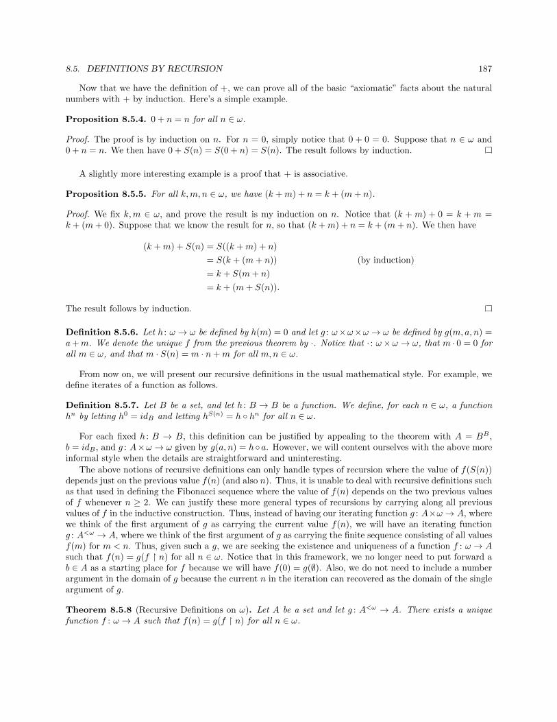
8.5. DEFINITIONS BY RECURSION 187
Now that we have the definition of +, we can prove all of the basic “axiomatic” facts about the naturalnumbers with + by induction. Here’s a simple example.
Proposition 8.5.4. 0 + n = n for all n ∈ ω.
Proof. The proof is by induction on n. For n = 0, simply notice that 0 + 0 = 0. Suppose that n ∈ ω and0 + n = n. We then have 0 + S(n) = S(0 + n) = S(n). The result follows by induction.
A slightly more interesting example is a proof that + is associative.
Proposition 8.5.5. For all k,m, n ∈ ω, we have (k +m) + n = k + (m+ n).
Proof. We fix k,m ∈ ω, and prove the result is my induction on n. Notice that (k + m) + 0 = k + m =k + (m+ 0). Suppose that we know the result for n, so that (k +m) + n = k + (m+ n). We then have
(k +m) + S(n) = S((k +m) + n)
= S(k + (m+ n)) (by induction)
= k + S(m+ n)
= k + (m+ S(n)).
The result follows by induction.
Definition 8.5.6. Let h : ω → ω be defined by h(m) = 0 and let g : ω×ω×ω → ω be defined by g(m, a, n) =a+m. We denote the unique f from the previous theorem by ·. Notice that · : ω×ω → ω, that m · 0 = 0 forall m ∈ ω, and that m · S(n) = m · n+m for all m,n ∈ ω.
From now on, we will present our recursive definitions in the usual mathematical style. For example, wedefine iterates of a function as follows.
Definition 8.5.7. Let B be a set, and let h : B → B be a function. We define, for each n ∈ ω, a functionhn by letting h0 = idB and letting hS(n) = h ◦ hn for all n ∈ ω.
For each fixed h : B → B, this definition can be justified by appealing to the theorem with A = BB ,b = idB , and g : A×ω → ω given by g(a, n) = h ◦a. However, we will content ourselves with the above moreinformal style when the details are straightforward and uninteresting.
The above notions of recursive definitions can only handle types of recursion where the value of f(S(n))depends just on the previous value f(n) (and also n). Thus, it is unable to deal with recursive definitions suchas that used in defining the Fibonacci sequence where the value of f(n) depends on the two previous valuesof f whenever n ≥ 2. We can justify these more general types of recursions by carrying along all previousvalues of f in the inductive construction. Thus, instead of having our iterating function g : A×ω → A, wherewe think of the first argument of g as carrying the current value f(n), we will have an iterating functiong : A<ω → A, where we think of the first argument of g as carrying the finite sequence consisting of all valuesf(m) for m < n. Thus, given such a g, we are seeking the existence and uniqueness of a function f : ω → Asuch that f(n) = g(f � n) for all n ∈ ω. Notice that in this framework, we no longer need to put forward ab ∈ A as a starting place for f because we will have f(0) = g(∅). Also, we do not need to include a numberargument in the domain of g because the current n in the iteration can recovered as the domain of the singleargument of g.
Theorem 8.5.8 (Recursive Definitions on ω). Let A be a set and let g : A<ω → A. There exists a uniquefunction f : ω → A such that f(n) = g(f � n) for all n ∈ ω.

188 CHAPTER 8. DEVELOPING BASIC SET THEORY
Proof. We first prove existence. Call a set Z ⊆ ω × A sufficient if for all n ∈ ω and all q ∈ An such that(k, q(k)) ∈ Z for all k < n, we have (n, g(q)) ∈ Z. Notice that sufficient sets exists (since ω×A is sufficient).Let
Y = {(n, a) ∈ ω ×A : (n, a) ∈ Z for every sufficient set Z}.
We first show that Y is sufficient. Let n ∈ ω and q ∈ An be arbitrary such that (k, q(k)) ∈ Y for all k < n.For any sufficient set Z, we have (k, q(k)) ∈ Z for all k < n, so (n, g(q)) ∈ Z. Therefore, (n, g(q)) ∈ Z forevery sufficient set Z, so (n, g(q)) ∈ Y . It follows that Y is sufficient.
We next show that for all n ∈ ω, there exists a unique a ∈ A such that (n, a) ∈ Y . Let
X = {n ∈ ω : There exists a unique a ∈ A such that (n, a) ∈ Y }.
Let n ∈ ω be arbitrary such that k ∈ X for all k < n. Let q = Y ∩ (n × A) and notice that q ∈ An. Since(k, q(k)) ∈ Y for all k < n and Y is sufficient, it follows that (n, g(q)) ∈ Y . Let b ∈ A be arbitrary withb 6= g(q). We then have that Y \{(n, b)} is sufficient (otherwise, there exists p ∈ An such that (k, p(k)) ∈ Yfor all k < n and g(p) = b, but this implies that p = q and hence b = a), so by definition of Y it follows thatY ⊆ Y \{(n, b)}. Hence, (n, b) /∈ Y . Therefore, there exists a unique a ∈ A such that (n, a) ∈ Y , so n ∈ X.
By induction, we conclude that X = ω, so for all n ∈ ω, there exists a unique a ∈ A such that (n, a) ∈ Y .Let f = Y and notice that f : ω → A because X = ω. Let n ∈ ω be arbitrary. Let q = Y ∩(n×A) and noticethat q ∈ An and q = f � n. Since (k, q(k)) ∈ Y for all k < n and Y is sufficient, it follows that (n, g(q)) ∈ Y ,so f(n) = g(q) = g(f � n).
We now prove uniqueness. Suppose that f1, f2 : ω → A are arbitrary functions with the following prop-erties:
1. f1(n) = g(f1 � n) for all n ∈ ω.
2. f2(n) = g(f2 � n) for all n ∈ ω.
Let X = {n ∈ ω : f1(n) = f2(n)}. We prove by induction that X = ω. Let n ∈ ω be arbitrary such thatk ∈ X for all k < n. We then have that f1 � n = f2 � n, hence
f1(n) = g(f1 � n)
= g(f2 � n)
= f2(n),
hence n ∈ X. It follows by induction that X = ω, so f1(n) = f2(n) for all n ∈ ω. Therefore, f1 = f2.
As above, there is a similar version when we allow parameters. If f : P × ω → A and p ∈ P , we use thenotation fp to denote the function fp : ω → A given by fp(n) = f(p, n) for all n ∈ ω.
Theorem 8.5.9 (Recursive Definitions with Parameters on ω). Let A and P be sets and let g : P×A<ω → A.There exists a unique function f : P × ω → A such that f(p, n) = g(p, fp � n) for all p ∈ P and n ∈ ω.
Proof. Similar to the proof of Theorem 8.5.2.
8.6 Infinite Sets and Infinite Powers
Theorem 8.6.1 (Cantor-Schroder-Bernstein). Let A and B be sets. If A � B and B � A, then A ≈ B.
Proof. We may assume that A and B are disjoint (otherwise, we can work with A× {0} and B × {1}, andtransfer the result back to A and B). Fix injections f : A→ B and g : B → A. We say that an element a ∈ Ais B-originating if there exists b0 ∈ B and n ∈ ω such that b0 /∈ range(f) and a = (g ◦ f)n(g(b0)). Similarly,

8.6. INFINITE SETS AND INFINITE POWERS 189
we say that an element b ∈ B is B-originating if there exists b0 ∈ B and n ∈ ω such that b0 /∈ range(f) andb = (f ◦ g)n(b0). Let
h = {(a, b) ∈ A×B : Either a is not B-originating and f(a) = b or a is B-originating and g(b) = a}.
Notice that h is a function (because f is a function and g is injective), domain(h) ⊆ A, and range(h) ⊆ B.We first show that domain(h) = A. Let a ∈ A be arbitrary. If a is not B-originating, then (a, f(a)) ∈ h,hence a ∈ domain(h). Suppose that a is B-originating, and fix b0 ∈ B and n ∈ ω with a = (g ◦ f)n(g(b0)).If n = 0, then a = g(b0), so (a, b0) ∈ h and hence a ∈ domain(h). Suppose that n 6= 0 and fix m ∈ ω withn = S(m). We then have
a = (g ◦ f)S(m)(g(b0))
= (g ◦ f)(((g ◦ f)m(g(b0))))
= g(f((g ◦ f)m(g(b0)))).
Therefore, (a, f((g ◦ f)m(g(b0)))) ∈ h, and hence a ∈ domain(h). It follows that domain(h) = A.We now know that h : A→ B, and we need only show that h is a bijection. Let a1, a2 ∈ A be arbitrary
with h(a1) = h(a2). We first show that either a1 and a2 are both B-originating or both a1 and a2 areboth not B-originating. Without loss of generality, suppose that a1 is B-originating and a2 is not, so thata1 = g(h(a1)) and h(a2) = f(a2). Since a1 is B-originating, we may fix b0 ∈ B and n ∈ ω such thatb0 /∈ range(f) and a1 = (g ◦ f)n(g(b0)). Notice that
(g ◦ f)n(g(b0)) = a1
= g(h(a1))
= g(h(a2))
= g(f(a2))
= (g ◦ f)(a2).
If n = 0, this implies that g(b0) = g(f(a2)), hence f(a2) = b0 (because g is injective), contrary to the factthat b0 /∈ range(f). Suppose that n 6= 0 and fix m ∈ ω with S(m) = n. We then have
(g ◦ f)((g ◦ f)m(g(b0))) = (g ◦ f)n(g(b0))
= (g ◦ f)(a2),
hence (g ◦ f)m(g(b0)) = a2 (because g ◦ f is injective), contrary to the fact that a2 is not B-originating.Therefore, either a1 and a2 are both B-originating or both a1 and a2 are both not B-originating. If a1 anda2 are both not B-originating, this implies that f(a1) = f(a2), hence a1 = a2 because f is injective. If a1
and a2 are both B-originating, we then have a1 = g(h(a1)) = g(h(a2)) = a2. It follows that h is injective.We finally show that h is surjective. Fix b ∈ B. Suppose first that b is B-originating, and fix b0 ∈ B and
n ∈ ω such that b0 /∈ range(f) and b = (f ◦ g)n(b0). We then have g(b) = g((f ◦ g)n(b0)) = (g ◦ f)n(g(b0)),hence g(b) ∈ A is B-originating. It follows that h(g(b)) = b, so b ∈ range(h). Suppose now that b isnot B-originating. We then must have b ∈ range(f), so we may fix a ∈ A with f(a) = b. If a is B-originating, we may fix b0 ∈ B and n ∈ ω such that b0 /∈ range(f) and a = (g ◦ f)n(g(b0)), and notice that(f ◦ g)S(n)(b0) = f((g ◦ f)n(g(b0))) = f(a) = b, contrary to the fact that b is not B-originating. Therefore,a is not B-originating, so h(a) = f(a) = b, and hence b ∈ range(h). It follows that h is surjective.
Definition 8.6.2. Let A and B be sets. We write A ≺ B to mean that A � B and A 6≈ B.
Definition 8.6.3. Let A be a set.
1. A is countably infinite if A ≈ ω.

190 CHAPTER 8. DEVELOPING BASIC SET THEORY
2. A is countable if A is either finite or countably infinite.
3. A is uncountable if A is not countable.
Proposition 8.6.4. Let A be a set. The following are equivalent:
1. A is countable.
2. A � ω.
3. There is a surjection g : ω → A.
Proof. Exercise.
Given a set A and an natural number n ∈ ω, we defined An be the set of all functions from n to A. Infact, there is no reason to restrict to powers that are natural numbers. In general, we want to define AB tobe the set of all functions from B to A. We can certainly make this definition, but it is the first instancewhere we really need to use Power Set.
Proposition 8.6.5. Let A and B be sets. There is a unique set, denoted by AB, such that for all f , wehave f ∈ AB if and only if f : B → A.
Proof. Notice that if f : B → A, then f ⊆ B ×A, hence f ∈ P(B ×A). Therefore, AB = {f ∈ P(B ×A) : fis a function, domain(f) = B, and range(f) = A}. As usual, uniqueness follows from Extensionality.
Theorem 8.6.6. For any set A, we have A ≺ P(A).
Proof. First, define a function f : A → P(A) by letting f(a) = {a} for every a ∈ A. Notice that f is aninjection, hence A � P(A). We next show that A 6≈ P(A) by showing that there is no bijection f : A→ P(A).SLet f : A → P(A) be an arbitrary function. Let B = {a ∈ A : a /∈ f(a)}, and notice that B ∈ P(A).Suppose that B ∈ range(f), and fix b ∈ A with f(b) = B. We then have b ∈ f(b) ↔ b ∈ B ↔ b /∈ f(b), acontradiction. It follows that B /∈ range(f), hence f is not surjective. Therefore, A ≺ P(A).
Chapter 9
Well-Orderings, Ordinals, andCardinals
9.1 Well-Orderings
The ability to do induction and make definitions by recursion on ω was essential to developing the basicproperties of the natural numbers. With such success, we now want to push inductive arguments andrecursive constructions to other structures. In Chapter 2, we successfully generalized the ”step” versionsof induction and recursive to other contexts where we generate elements one at a time. Now, we seek togeneralize the ”order” versions. The key property underlying the order versions is the fact that < is awell-ordering on ω. In fact, it is straightforward to see translate order induction to any well-ordering.
Proposition 9.1.1 (Induction on Well-Orderings). Let (W,<) be a well-ordering.
1. Suppose that X is set and for all z ∈W , if y ∈ X for all y < z, then z ∈ X. We then have W ⊆ X.
2. For any formula ϕ(z,~p), we have the sentence
∀~p((∀z ∈W )((∀y < z)ϕ(y,~p)→ ϕ(z,~p))→ (∀z ∈W )ϕ(z,~p))
3. Suppose that C is a class and for all z ∈W , if y ∈ C for all y < z, then z ∈ C. We then have W ⊆ C.
Proof.
1. Suppose that W * X so that W\X 6= ∅. Since (W,<) is a well-ordering, there exists z ∈ W\X suchthat for all y ∈ W\X, either z = y or z < y. Therefore, for all y ∈ W with y < z, we have y ∈ X(because y /∈ W\X). It follows from assumption that z ∈ X, contradicting the fact that z ∈ W\X.Thus, it must be the case that W ⊆ X.
2. This follows from part 1 using Separation. Fix sets ~q, and suppose that
(∀z ∈W )((∀y < z)ϕ(y, ~q)→ ϕ(z, ~q))
Let X = {z ∈ W : ϕ(n, ~q)}. Suppose that z ∈ W and y ∈ X for all y < z. We then have(∀y < z)ϕ(y, ~q), hence ϕ(z, ~q) by assumption, so z ∈ X. It follows from part 1 that W ⊆ X. Therefore,we have (∀z ∈W )ϕ(z, ~q).
3. This is just a restatement of 2 using the language of classes.
191

192 CHAPTER 9. WELL-ORDERINGS, ORDINALS, AND CARDINALS
This is all well and good, but are there other interesting well-orderings other than ω (and every n ∈ ω)?Well, any well-ordering has a smallest element. If there are any elements remaining, there must be a nextsmallest element. Again, if there are any elements remaining, there must be a next smallest element, and soon. In other words, any infinite well-ordering begins with a piece that looks like ω.
However, we can build another “longer” well-ordering by taking ω, and adding a new element which isgreater than every element of ω. This can be visualized by thinking of the following subset of R:
A =
{1− 1
n: n ∈ ω\{0}
}∪ {1}.
It’s a simple exercise to check that A, ordered by inheritance from the usual order on R, is a well-ordering.We can then add another new element which is greater than every element, and another and another andso on, to get a well-ordering that is a copy of ω with another copy of ω on top of the first. We can add anew element greater than all of these, and continue. These well-orderings “beyond” ω differ from ω (and alln ∈ ω) in that they have points that are neither initial points nor immediate successors of other points.
Definition 9.1.2. Let (W,<) be a well-ordering, and let z ∈W .
1. If z ≤ y for all y ∈W , we call z the initial point (such a z is easily seen to be unique).
2. If there exists y ∈W such that there is no x ∈W with y < x < z, we call z a successor point.
3. If z is neither an initial point nor a successor point, we call z a limit point.
A little thought will suggest that all well-orderings should be built up by starting at an initial point,taking successors (perhaps infinitely often), and then jumping to a limit point above everything previously.After all, if we already have an initial part that looks like ω, and we haven’t exhausted the well-ordering,then there must be a least element not accounted for, and this is the first limit point. If we still haven’texhausted it, there is another least element, which is a successor, and perhaps another successor, and so on.If this doesn’t finish off the well-ordering, there is another least element not accounted for which will be thesecond limit point. For example, as a subset of the real line, the set
A =
{1− 1
n: n ∈ ω\{0}
}∪{
2− 1
n: n ∈ ω\{0}
}∪ {2}.
is a well-ordering (under the inherited ordering from R) with two limit points (namely 1 and 2).This idea makes it seem plausible that we can take any two well-orderings and compare them by running
through this procedure until one of them runs out of elements. That is, if (W1, <1) and (W2, <2) are well-orderings, then either they are isomorphic, or one is isomorphic to an initial segment of the other. We nowdevelop the tools to prove this result. We first show that we can make recursive definitions along well-orderings. The proof is basically the same as the proof of the Induction Principle on ω because the onlyimportant fact that allowed that argument to work was the property of the order < on ω (not the fact thatevery element of ω was either an initial point or a successor point).
Definition 9.1.3. Let (W,<) be a well-ordering, and let z ∈W . We let W (z) = {y ∈W : y < z}.
Definition 9.1.4. Let (W,<) be a well-ordering. A set I ⊆ W is called an initial segment of W if I 6= Wand whenever x ∈ I and y < x, we have y ∈ I.
Proposition 9.1.5. Suppose that (W,<) is a well-ordering and I is an initial segment of W . There existsz ∈W with I = W (z).

9.1. WELL-ORDERINGS 193
Proof. Since I is an initial segment of W , we have I ⊆W and I 6= W . Therefore, W\I 6= ∅. Since (W,<) isa well-ordering, there exists z ∈W\I such that z ≤ y for all y ∈W\I. We claim that I = W (z).
• Let y ∈W (z) be arbitrary. Since y < z, we then have y /∈W\I, so y ∈ I. Therefore, W (z) ⊆ I.
• Let y ∈ I be arbitrary with y /∈W (z). We then have y 6< z, so y ≥ z because < is a well-ordering (andhence a linear ordering). Therefore, z ∈ I because I is an initial segment, contradicting the fact thatz ∈W\I. It follows that I ⊆W (z).
Combining these, it follows from Extensionality that I = W (z).
Definition 9.1.6. Let (W,<) be a well-ordering and let A be a set. We let
A<W = {f ∈ P(W ×A) : f is a function and f : W (z)→ A for some z ∈W}.
Theorem 9.1.7 (Recursive Definitions on Well-Orderings). Let (W,<) be a well-ordering, let A be a set,and let g : A<W → A. There exists a unique function f : W → A such that f(z) = g(f � W (z)) for allz ∈W .
Proof. We first prove existence. Call a set Z ⊆W ×A sufficient if for all z ∈W and all q ∈ AW (z) such that(y, q(y)) ∈ Z for all y < z, we have (z, g(q)) ∈ Z. Notice that sufficient sets exists (since W ×A is sufficient).Let
Y = {(z, a) ∈W ×A : (z, a) ∈ Z for every sufficient set Z}.
We first show that Y is sufficient. Let z ∈ W and q ∈ AW (z) be arbitrary such that (y, q(y)) ∈ Y for ally < z. For any sufficient set Z, we have (y, q(y)) ∈ Z for all y < z, so (z, g(q)) ∈ Z. Therefore, (z, g(q)) ∈ Zfor every sufficient set Z, so (z, g(q)) ∈ Y . It follows that Y is sufficient.
We next show that for all z ∈W , there exists a unique a ∈ A such that (z, a) ∈ Y . Let
X = {z ∈W : There exists a unique a ∈ A such that (z, a) ∈ Y }.
Let z ∈ W be arbitrary such that y ∈ X for all y < z. Let q = Y ∩ (W (z)× A) and notice that q ∈ AW (z).Since (y, q(y)) ∈ Y for all y < z and Y is sufficient, it follows that (z, g(q)) ∈ Y . Fix b ∈ A with b 6= g(q).We then have that Y \{(z, b)} is sufficient (otherwise, there exists p ∈ AW (z) such that (y, p(y)) ∈ Y for ally < z and g(p) = b, but this implies that p = q and hence b = a), so by definition of Y it follows thatY ⊆ Y \{(z, b)}. Hence, (z, b) /∈ Y . Therefore, there exists a unique a ∈ A such that (z, a) ∈ Y , so z ∈ X.
By induction, we conclude that X = W , so for all z ∈W , there exists a unique a ∈ A such that (z, a) ∈ Y .Let f = Y and notice that f : W → A because X = ω. Let z ∈W be arbitrary. Define q ∈ AW (z) by lettingq = Y ∩ (W (z) × A) and notice that q = f � W (z). Since (y, q(y)) ∈ Y for all y < z and Y is sufficient, itfollows that (z, g(q)) ∈ Y , so f(z) = g(q) = g(f �W (z)).
We now prove uniqueness. Suppose that f1, f2 : W → A are arbitrary functions with the followingproperties:
1. f1(z) = g(f1 �W (z)) for all z ∈ ω.
2. f2(z) = g(f2 �W (z)) for all z ∈ ω.
Let X = {z ∈W : f1(z) = f2(z)}. We prove by induction that X = W . Let z ∈W and suppose that y ∈ Xfor all y < z. We then have that f1 �W (z) = f2 �W (z), hence
f1(z) = g(f1 �W (z))
= g(f2 �W (z))
= f2(z),
hence z ∈ X. It follows by induction that X = W , so f1(z) = f2(z) for all z ∈W . Therefore, f1 = f2.

194 CHAPTER 9. WELL-ORDERINGS, ORDINALS, AND CARDINALS
Definition 9.1.8. Let (W1, <1) and (W2, <2) be well-orderings.
1. A function f : W1 →W2 is order-preserving if whenever x, y ∈W1 and x <1 y, we have f(x) <2 f(y).
2. A function f : W1 →W2 is an isomorphism if it is bijective and order-preserving.
3. If W1 and W2 are isomorphic, we write W1∼= W2.
Proposition 9.1.9. Suppose that (W,<) is a well-ordering and f : W → W is order-preserving. We thenhave f(z) ≥ z for all z ∈W .
Proof. We prove the result by induction on W . Suppose that z ∈ W and f(y) ≥ y for all y < z. Supposeinstead that f(z) < z, and let x = f(z). Since f is order-preserving and x < z, it follows that f(x) <f(z) = x, contradicting the fact that f(y) ≥ y for all y < z. Therefore, f(z) ≥ z. The result follows byinduction.
Proposition 9.1.10. Let (W1, <1) and (W2, <2) be well-orderings. If f : W1 → W2 is an isomorphism,then f−1 : W2 →W1 is also an isomorphism.
Proof. Exercise.
Corollary 9.1.11.
1. If (W,<) is a well-ordering and z ∈W , then W �W (z).
2. If (W,<) is a well-ordering, then its only automorphism is the identity.
3. If (W1, <1) and (W2, <2) are well-orderings, and W1∼= W2, then the isomorphism from W1 to W2 is
unique.
Proof.
1. Suppose that W ∼= W (z) for some z ∈ W and let f : W → W (z) be a witnessing isomorphism. Thenf : W →W is order-preserving and f(z) < z (because f(z) ∈W (z)), contrary to Proposition 9.1.9.
2. Let f : W → W be an arbitrary automorphism of W . Let z ∈ W be arbitrary. By Proposition 9.1.9,we have f(z) ≥ z. Since f−1 : W → W is also an automorphism of W , Proposition 9.1.9 implies thatf−1(f(z)) ≥ f(z), hence z ≥ f(z). Combining f(z) ≥ z and z ≥ f(z), we conclude that z = f(z).Since z ∈W was arbitrary, we conclude that f is the identity function.
3. Suppose that f : W1 →W2 and g : W1 →W2 are both isomorphisms. We then have that g−1 : W2 →W1
is an isomorphism, hence g−1 ◦ f : W1 →W1 is an automorphism. Hence, by part b, we may concludethat g−1 ◦ f is the identity on W1. It follows that f = g.
Theorem 9.1.12. Let (W1, <1) and (W2, <2) be well-orderings. Exactly one of the following holds:
1. W1∼= W2.
2. There exists z ∈W2 such that W1∼= W2(z).
3. There exists z ∈W1 such that W1(z) ∼= W2.
In each of the above cases, the isomorphism and the z (if appropriate) are unique.

9.2. ORDINALS 195
Proof. We first prove that one of the three options holds. Fix a set a such that a /∈ W1 ∪ W2 (such ana exists by Proposition 8.1.4). Our goal is to define a function f : W1 → W2 ∪ {a} recursively. Defineg : (W2 ∪ {a})<W1 → W2 ∪ {a} as follows. Let q ∈ (W2 ∪ {a})<W1 be arbitrary, and fix z ∈ W1 such thatq : W1(z) → W2 ∪ {a}. If a ∈ range(q) or range(q) = W2, let g(q) = a. Otherwise range(q) is a propersubset of W2, and we let g(q) be the <2-least element of W2\range(q). By Theorem 9.1.7, there is a uniquef : W1 →W2 ∪ {a} such that f(z) = g(f �W1(z)) for all z ∈W1.
Suppose first that a /∈ range(f) so that f : W1 → W2. We begin by showing that range(f � W1(z)) is aninitial segment of W2 for all z ∈W1 by induction. Let z ∈W1 be arbitrary such that range(f �W1(y)) is aninitial segment of W2 for all y < z. We have three cases:
• Case 1: Suppose that z is the initial point of W1. We then range(f �W1(z)) = ∅ is certainly an initialsegment of W2.
• Case 2: Suppose that z is a successor point of W1. Fix y ∈ W1 such that there is no x ∈ W1
with y < x < z. By induction, we know that range(f � W1(y)) is an initial segment of W2. Sincef(y) = g(f �W1(y)) is the <2-least element of W2\range(f �W1(y)), it follows that range(f �W1(z)) =range(f �W1(y)) ∪ {f(y)} is an initial segment of W2.
• Case 3: Suppose finally that z is a limit point of W1. It then follows that range(f � W1(z)) =⋃y<z range(f � W1(y)). Since every element of the union is an initial segment of W2, it follows that
range(f �W1(z)) is an initial segment of W2 (note that it can’t equal W2 because f(z) 6= a).
Therefore, range(f � W1(z)) is an initial segment of W2 for all z ∈ W1 by induction. It follows that forall y, z ∈ W1 with y < z, we have f(y) < f(z) (because range(f � W1(z)) is an initial segment of W1 andf(y) ∈ range(f �W1(z))), so f is order-preserving. This implies that f is an injection, so if range(f) = W2,we have W1
∼= W2. Otherwise, range(f) is an initial segment of W2, so by Proposition 9.1.5 there is a z ∈W2
such that W1∼= W2(z).
Suppose now that a ∈ range(f). Let z ∈ W1 be the <1-least element of W1 such that f(z) = a. Itthen follows that f � W1(z) : W1(z) → W2 is order-preserving by induction as above. Also, we must haverange(f � W1(z)) = W2 because f(z) = a. Therefore, f � W1(z) : W1(z) → W2 is an isomorphism. Thiscompletes the proof that one of the above 3 cases must hold.
The uniqueness of the case, the isomorphism, and the z (if appropriate), all follow from Corollary 9.1.11
With this result in hand, we now know that any well-ordering is uniquely determined by its “length”.The next goal is to find a nice system of representatives for the isomorphism classes of well-orderings. Forthat, we need to generalize the ideas that went into the construction of the natural numbers.
9.2 Ordinals
Our definition of the natural numbers had the advantage that the ordering was given by the membershiprelation ∈. This feature allowed us to define successors easily and to think of a natural number n as theset of all natural numbers less than n. We now seek to continue this progression to measure well-orderingslonger than ω. The idea is to define successors as in the case of the natural numbers, but now to take unionsto achieve limit points.
The key property of ω (and each n ∈ ω) that we want to use in our definition of ordinals is the fact that∈ well-orders ω (and each n ∈ ω). We need one more condition to ensure that there are no “holes” or “gaps”in the set. For example, ∈ well-orders the set {0, 2, 3, 5}, but we don’t want to consider it as an ordinalbecause it skipped over 1 and 4. We therefore make the following definition.
Definition 9.2.1. A set z is transitive if whenever x and y are sets such that x ∈ y and y ∈ z, we havex ∈ z.

196 CHAPTER 9. WELL-ORDERINGS, ORDINALS, AND CARDINALS
Definition 9.2.2. Let z be a set. We define a relation ∈z on z by setting ∈z= {(x, y) ∈ z × z : x ∈ y}.
Definition 9.2.3. An ordinal is a set α which is transitive and well-ordered by ∈α.
Our hard work developing the natural numbers gives us one interesting example of an ordinal.
Proposition 9.2.4. ω is an ordinal.
Proof. Proposition 8.2.11 says that ω is transitive, and Theorem 8.2.18 says that ω is well-ordered by< = ∈ω.
Proposition 9.2.5. If α is an ordinal and β ∈ α, then β is an ordinal.
Proof. We first show that β is transitive. Let x and y be sets with x ∈ y and y ∈ β. Since y ∈ β, β ∈ α, andα is transitive, it follows that y ∈ α. Since x ∈ y and y ∈ α, it follows that x ∈ α. Now since x, y, β ∈ α,x ∈ y, y ∈ β, and ∈α is transitive on α, we may conclude that x ∈ β. Therefore, β is transitive.
Notice that β ⊆ α because β ∈ α and α is transitive. Therefore, ∈β is the restriction of ∈α to the subsetβ ⊆ α. Since ∈α is a well-ordering on α, it follows that ∈β is a well-ordering on β. Hence, β is an ordinal.
Corollary 9.2.6. Every n ∈ ω is an ordinal.
Lemma 9.2.7. If α is an ordinal, then α /∈ α.
Proof. Suppose that α is an ordinal and α ∈ α. Since α ∈ α, it follows that ∈α is not asymmetric on α,contradicting the fact that ∈α is a well-ordering on α.
Proposition 9.2.8. If α is an ordinal, then S(α) is an ordinal.
Proof. We first show that S(α) is transitive. Suppose that x ∈ y ∈ S(α). Since y ∈ S(α) = α ∪ {α}, eithery ∈ α or y = α. Suppose first that y ∈ α. We then have x ∈ y ∈ α, so x ∈ α because α is transitive. Hence,x ∈ S(α). Suppose now that y = α. We then have x ∈ α because x ∈ y, so x ∈ S(α).
We next show that ∈S(α) is transitive on S(α). Let x, y, z ∈ S(α) with x ∈ y ∈ z. Since z ∈ S(α), eitherz ∈ α or z = α. Suppose first that z ∈ α. We then have y ∈ α (since y ∈ z ∈ α and α is transitive), andhence x ∈ α (since x ∈ y ∈ α and α is transitive). Thus, x, y, z ∈ α, so we may conclude that x ∈ z usingthe fact that ∈α is transitive on α. Suppose now that z = α. We then have x ∈ α = z because x ∈ y ∈ αand α is transitive.
We next show that ∈S(α) is asymmetric on S(α). Let x ∈ S(α). If x ∈ α, then x /∈ x because ∈α isasymmetric on α. If x = α, then x /∈ x by Lemma 9.2.7.
We now show that ∈S(α) is connected on S(α). Let x, y ∈ S(α). If x ∈ α and y ∈ α, then either x ∈ y,x = y, or y ∈ x because ∈α is connected on α. If x = α and y = α, we clearly have x = y. Otherwise, oneof x, y equals α, and the other is an element of α, if which case we’re done.
Finally, suppose that X ⊆ S(α) and X 6= ∅. If X ∩ α = ∅, then we must have X = {α}, in which caseX clearly has a ∈S(α)-least element. Suppose that X ∩ α 6= ∅. Since X ∩ α ⊆ α is nonempty and ∈α is awell-ordering on α, there exists a ∈α-least element β in X ∩α. For any γ ∈ X, either γ ∈ α in which case wehave have either β = γ or β ∈ γ by choice of β, or γ = α in which case β ∈ γ (because β ∈ α). Therefore,X has a ∈S(α)-least element.
Proposition 9.2.9. Suppose that α and β are ordinals. We then have α ⊆ β if and only if either α = β orα ∈ β.
Proof. (⇐) If α = β, then clearly α ⊆ β and if α ∈ β we can use the fact that β is transitive to concludethat α ⊆ β.
(⇒) Suppose that α ⊆ β and α 6= β. Notice that β\α is an nonempty subset of β, so there exists a∈β-least element of β\α, call it z. We show that α = z, hence α ∈ β. We first show that z ⊆ α. Let x ∈ z.

9.2. ORDINALS 197
Since z ∈ β and β is transitive, we have x ∈ β. Since x ∈ z, we can not have x ∈ β\α by choice of z, sox ∈ α. Thus, z ⊆ α. We next show that α ⊆ z. Let x ∈ α. Since α ⊆ β, we have x ∈ β. Using the factthat x, z ∈ β and ∈β is connected on β, we know that either x ∈ z, x = z, or z ∈ x. We can not have x = zbecause x ∈ α and z ∈ β\α. Also, we can not have z ∈ x, because if z ∈ x we can also conclude that z ∈ α(because z ∈ x ∈ α and α is transitive), contradicting the fact that z ∈ β\α. Thus, α ⊆ z. It follows thatz = α (by Extensionality), so α ∈ β.
Proposition 9.2.10. Suppose that α and β are ordinals. Exactly one of α ∈ β, α = β, or β ∈ α holds.
Proof. We first show that at least one of α ∈ β, α = β, β ∈ α holds. We first claim that α∩ β is an ordinal.If x ∈ y ∈ α ∩ β, then x ∈ y ∈ α and x ∈ y ∈ β, so x ∈ α and x ∈ β (because α and β are transitive), andhence x ∈ α∩β. Thus, α∩β is transitive. Notice that ∈α∩β is the restriction of ∈α to the subset α∩β ⊆ α.Since ∈α is a well-ordering on α, it follows that ∈α∩β is a well-ordering on α∩ β. Hence, α∩ β is an ordinal.
Now we have α ∩ β ⊆ α and α ∩ β ⊆ β. If α ∩ β 6= α and α ∩ β 6= β, then α ∩ β ∈ α and α ∩ β ∈ β byProposition 9.2.9, hence α ∩ β ∈ α ∩ β, contrary to Lemma 9.2.7. Therefore, either α ∩ β = α or α ∩ β = β.If α∩ β = α, we then have α ⊆ β, hence either α = β or α ∈ β by Proposition 9.2.9. Similarly, if α∩ β = β,we then have β ⊆ α, hence either β = α or β ∈ α by Proposition 9.2.9. Thus, in any case, at least one α ∈ β,α = β, or β ∈ α holds.
We finish by showing that exactly one of α ∈ β, α = β, or β ∈ α holds. If α ∈ β and α = β, then α ∈ α,contrary to Lemma 9.2.7. Similarly, if α = β and β ∈ α, then β ∈ β, contrary to Lemma 9.2.7. Finally, ifα ∈ β and β ∈ α, then α ∈ α (because α is transitive), contrary to Lemma 9.2.7.
Definition 9.2.11. If α and β are ordinals, we write α < β to mean that α ∈ β.
Proposition 9.2.12. Let α and β be arbitrary ordinals. We have α < S(β) if and only if α ≤ β.
Proof. Notice that S(β) is an ordinal by Proposition 9.2.8. Now
α < S(β)⇔ α ∈ S(β)
⇔ α ∈ β ∪ {β}⇔ Either α ∈ β or α ∈ {β}⇔ Either α < β or α = β
⇔ α ≤ β.
Proposition 9.2.13. Suppose that α and β are ordinals. If α ∼= β as well-orderings, then α = β.
Proof. If α 6= β, then either α < β or β < α by Proposition 9.2.10. Suppose without loss of generality thatβ < α. We then have that the well-ordering β is an initial segments of the well-ordering α (in the notationfor well-orderings, we have β = α(β)), hence α � β by Corollary 9.1.11.
By the above results, it seems that we are in a position to say that < is a linear ordering on the collectionof all ordinals. However, there is a small problem here. We do not know that the class of all ordinals is aset. In fact, we will see below that the collection of all ordinals is a proper class.
Definition 9.2.14. ORD is the class of all ordinals.
We first establish that nonempty sets of ordinals have least elements.
Proposition 9.2.15. If A is a nonempty subset of ORD, then A has a least element. Furthermore the leastelement is given by
⋂A.

198 CHAPTER 9. WELL-ORDERINGS, ORDINALS, AND CARDINALS
Proof. Since A 6= ∅, we may fix an ordinal α ∈ A. If A ∩ α = ∅, then for any β ∈ A, we can not have β ∈ α,hence either α = β or α ∈ β by Proposition 9.2.10. Suppose that A∩α 6= ∅. Since A∩α ⊆ α is nonempty, ithas an ∈α-least element, call it δ. Let β ∈ A and notice that β is an ordinal. By Proposition 9.2.10, eitherβ ∈ α, β = α, or α ∈ β. If β ∈ α, then β ∈ A ∩ α, so either δ = β or δ ∈ β by choice of δ. If β = α, thenδ ∈ β because δ ∈ α. If α ∈ β, we then have δ ∈ α ∈ β, so δ ∈ β because β is transitive. It follows that δ isthe least element of A.
Therefore, we know that A has a least element, call it δ. Since δ ∈ A, we certainly have⋂A ⊆ δ. For all
α ∈ A, we then have either δ = α or δ ∈ α, hence δ ⊆ α by Proposition 9.2.9. Therefore, δ ⊆⋂A. It follows
that δ =⋂A.
Proposition 9.2.16. If A is a subset of ORD, then⋃A is an ordinal. Furthermore, we have
⋃A = supA,
i.e. α ≤⋃A for all α ∈ A and
⋃A ≤ β whenever β is an ordinal with β ≥ α for all α ∈ A.
Proof. We first show that⋃A is transitive. Suppose that x ∈ y ∈
⋃A. Since y ∈
⋃A, there exists α ∈ A,
necessarily an ordinal, such that y ∈ α ∈ A. Since α is transitive and x ∈ y ∈ α, we can conclude that x ∈ α.It follows that x ∈
⋃A. Hence,
⋃A is transitive.
We next show that ∈⋃A is transitive on⋃A. Let x, y, z ∈
⋃A with x ∈ y ∈ z. Since z ∈
⋃A, there
exists α ∈ A, necessarily an ordinal, such that z ∈ α ∈ A. Since z ∈ α and α is an ordinal, we may useProposition 9.2.5 to conclude that z is an ordinal. Thus, z is transitive, so we may use the fact that x ∈ y ∈ zto conclude that x ∈ z.
We next show that ∈⋃A is asymmetric on⋃A. Let x ∈
⋃A and fix α ∈ A, necessarily an ordinal, such
that x ∈ α ∈ A. Using Proposition 9.2.5 again, it follows that x is an ordinal, hence x /∈ x by Lemma 9.2.7.We now show that ∈⋃A is connected on
⋃A. Let x, y ∈
⋃A. Fix α, β ∈ A, necessarily ordinals, such
that x ∈ α ∈ A and y ∈ β ∈ A. Again, using Proposition 9.2.5, we may conclude that x and y are ordinals,hence either x ∈ y, x = y, or y ∈ x by Proposition 9.2.10
Finally, suppose that X ⊆⋃A and X 6= ∅. Notice that for any y ∈ X, there exists α ∈ A, necessarily an
ordinal, such that y ∈ α ∈ A, and hence y is an ordinal by Proposition 9.2.10. Therefore, X is a nonemptysubset of ORD, so by Proposition 9.2.15 we may conclude that X has a least element (with respect to∈⋃A).
We now show that⋃A = supA. Suppose that α ∈ A. For any β ∈ α, we have β ∈ α ∈ A, hence
β ∈⋃A. It follows that α ⊆
⋃A, hence α ≤
⋃A by Proposition 9.2.9. Thus,
⋃A is an upper bound for A.
Suppose that γ is an upper bound for A, i.e. γ is an ordinal and α ≤ γ for all α ∈ A. For any β ∈⋃A, we
may fix α ∈ A such that β ∈ α and notice that β ∈ α ⊆ γ, so β ∈ γ. It follows that⋃A ⊆ γ, hence
⋃A ≤ γ
by Proposition 9.2.9. Therefore,⋃A = supA.
Proposition 9.2.17. ORD is a proper class.
Proof. Suppose that ORD is a set, so that there is a set O such that α is an ordinal if and only α ∈ O.In this case, O is a transitive set (by Proposition 9.2.5) which is well-ordered by ∈O (transitivity followsfrom the fact that ordinals are transitive sets, asymmetry follows from Lemma 9.2.7, connectedness followsfrom Proposition 9.2.10, and the fact that every nonempty subset has a least element is given by Proposition9.2.15). Therefore, O is an ordinal and so it follows that O ∈ O, contrary to Lemma 9.2.7. Hence, ORD isnot a set.
Since ORD is a proper class, there are subclasses of ORD which are not subsets of ORD. We thereforeextend Proposition 9.2.15 to the case of nonempty subclasses of ORD. The idea is that if we fix an α ∈ C,then α∩ C becomes a set of ordinals, so we can apply the above result.
Proposition 9.2.18. If C is a nonempty subclass of ORD, then C has a least element.
Proof. Since C 6= ∅, we may fix an ordinal α ∈ C. If C ∩α = ∅, then for any β ∈ C, we can not haveβ ∈ α, hence either α = β or α ∈ β by Proposition 9.2.10. Suppose that C ∩α 6= ∅. In this case, C ∩α is

9.2. ORDINALS 199
a nonempty set of ordinals by Separation, hence C ∩α has a least element δ by Proposition 9.2.15. It nowfollows easily that δ is the least element of C.
Proposition 9.2.19 (Induction on ORD). Suppose that C ⊆ ORD and that for all ordinals α, if β ∈ Cfor all β < α, then α ∈ C. We then have C = ORD.
Proof. Suppose that C ( ORD. Let B = ORD \ C and notice that B is a nonempty class of ordinals. ByProposition 9.2.18, it follows that B has a least element, call it α. For all β < α, we then have β /∈ B, henceβ ∈ C. By assumption, this implies that α ∈ C, a contradiction. It follows that C = ORD.
This gives a way to do “strong induction” on the ordinals, but there is a slightly more basic version.
Definition 9.2.20. Let α be an ordinal.
• We say that α is a successor ordinal if there exists an ordinal β with α = S(β).
• We say that α is a limit ordinal if α 6= 0 and α is not a successor ordinal.
Notice that α is a limit ordinal if and only if α 6= 0, and whenever β < α, we have S(β) < α. For example,ω is a limit ordinal. In an inductive argument, we can’t get around looking at many previous values at limitordinals, but we can by with just looking at the previous ordinal in the case of successors.
Proposition 9.2.21 (Step/Limit Induction on ORD). Suppose that C ⊆ ORD with the following proper-ties:
1. 0 ∈ C.
2. Whenever α ∈ C, we have S(α) ∈ C.
3. Whenever α is a limit ordinal and β ∈ C for all β < α, we have α ∈ C.
We then have C = ORD.
Proof. Suppose that C ( ORD. Let B = ORD \ C and notice that B is a nonempty class of ordinals. ByProposition 9.2.18, it follows that B has a least element, call it α. We can’t have α = 0 because 0 ∈ C. Also,it is not possible that α is a successor, say α = S(β), because if so, then β /∈ B (because β < α), so β ∈ C,hence α = S(β) ∈ C. Finally, suppose that α is a limit. Then for for all β < α, we have β /∈ B, hence β ∈C. By assumption, this implies that α ∈ C, a contradiction. It follows that C = ORD.
Theorem 9.2.22 (Recursive Definitions on ORD). Let G : V → V be a class function. There exists aunique class function F : ORD → V such that F(α) = G(F � α) for all α ∈ ORD.
Theorem 9.2.23 (Recursive Definitions with Parameters on ORD). Let P be a class and let G : P × V→ V be a class function. There exists a unique class function F : P × ORD → V such that F(p, α) =G(Fp � α) for all p ∈ P and all α ∈ ORD.
Theorem 9.2.24. Let (W,<) be a well-ordering. There exists a unique ordinal α such that W ∼= α.
Proof. Fix a set a such that a /∈ W (such an a exists by Proposition 8.1.4). We define a class function F :ORD →W ∪{a} recursively as follows. If a ∈ range(F � α) or range(F � α) = W , let F(α) = a. Otherwise,range(F � α) (W , and we let F(α) be the least element of W\range(F � α).
Since ORD is a proper class, it follows from Proposition 8.3.5 that F is not injective. From this it followsthat a ∈ range(F) (otherwise, a simple inductive proof gives that F would have to be injective). Let α bethe least ordinal such that F(α) = a. Now it is straightforward to prove (along the lines of the proof ofTheorem 9.1.12) that F � α : α→W is an isomorphism.
Uniqueness follows from Proposition 9.2.13
Definition 9.2.25. Let (W,<) be a well-ordering. The unique ordinal α such that W ∼= α is called theorder-type of (W,<).

200 CHAPTER 9. WELL-ORDERINGS, ORDINALS, AND CARDINALS
9.3 Arithmetic on Ordinals
Now that we have the ability to define functions recursively on all of the ordinals, we can extend ourdefinitions of addition, multiplication, and exponentiation of natural numbers into the transfinite.
Definition 9.3.1. We define ordinal addition (that is a class function +: ORD ×ORD → ORD) recur-sively as follows.
1. α+ 0 = α.
2. α+ S(β) = S(α+ β).
3. α+ β =⋃{α+ γ : γ < β} if β is a limit ordinal.
Similarly, we define ordinal multiplication recursively as follows.
1. α · 0 = 0.
2. α · S(β) = α · β + α.
3. α · β =⋃{α · γ : γ < β} if β is a limit ordinal.
Finally, we define ordinal exponentiation recursively as follows.
1. α0 = 1.
2. αS(β) = αβ · α.
3. αβ =⋃{αγ : γ < β} if β is a limit ordinal.
Notice that we have
ω + 1 = ω + S(0)
= S(ω + 0)
= S(ω).
On the other hand, since ω is a limit ordinal and + is commutative on ω (by the homework), we have
1 + ω =⋃{1 + n : n < ω}
=⋃{n+ 1 : n < ω}
=⋃{n+ S(0) : n < ω}
=⋃{S(n+ 0) : n < ω}
=⋃{S(n) : n ∈ ω}
= ω.
Therefore, we have ω + 1 6= 1 + ω, and hence addition of ordinals is not commutative in general. Moreover,notice that even though we have 0 < 1, we do not have 0 + ω < 1 + ω (because 0 + ω = ω as well. In otherwords, addition on the right does not preserve the strict ordering relation. In contrast, addition on the leftdoes preserve the ordering, as we now show. We start with the non-strict version.
Proposition 9.3.2. Let α, β, and γ be ordinals. If β ≤ γ, then α+ β ≤ α+ γ.

9.3. ARITHMETIC ON ORDINALS 201
Proof. Fix arbitrary ordinals α and β. We prove by induction on γ that if β ≤ γ, then α+ β ≤ α+ γ. Forthe base case, notice that the statement is trivial when γ = β. For the successor step, let γ ≥ β be arbitrarysuch that α+ β ≤ α+ γ. We then have
α+ β ≤ α+ γ
< S(α+ γ)
= α+ S(γ),
so the statement is true for S(γ). For the limit case, suppose that γ > β is a limit ordinal with the propertythat α+ β ≤ α+ δ whenever β ≤ δ < γ. We then have
α+ β ≤⋃{α+ δ : δ < γ} (since β < γ)
= α+ γ,
so the statement is true for γ. The result follows by induction.
Proposition 9.3.3. Let α, β, and γ be ordinals. We have β < γ if and only if α+ β < α+ γ.
Proof. Let α and β be arbitrary ordinals. Notice first that
α+ β < S(α+ β) = α+ S(β).
Now if γ is an arbitrary ordinal with γ > β, then we have S(β) ≤ γ, hence
α+ β < α+ S(β) ≤ α+ γ
by Proposition 9.3.2. Therefore, we have α + β < α + γ. For the converse, notice that if γ < β, thenα+ γ < α+ β by what we just proved.
Proposition 9.3.4. Let α and β be ordinals. If β is a limit ordinal, then α+ β is a limit ordinal.
Proof. Since β is a limit ordinal, we have
α+ β =⋃{α+ γ : γ < β}.
Let δ < α+ β be an arbitrary ordinal. We show that S(δ) < α+ β. We have
δ <⋃{α+ γ : γ < β},
so by Proposition 9.2.16, we can fix γ < β with δ < α+γ. Since β is a limit ordinal, we then have S(γ) < β,so
S(δ) ≤ α+ γ
< S(α+ γ)
= α+ S(γ)
≤ α+ β.
It follows that α+ β is a limit ordinal.
Proposition 9.3.5. For all ordinals α, β, and γ, we have (α+ β) + γ = α+ (β + γ).

202 CHAPTER 9. WELL-ORDERINGS, ORDINALS, AND CARDINALS
Proof. Fix ordinals α and β. We prove that (α+β)+γ = α+(β+γ) for all ordinals γ by induction. Supposefirst that γ = 0. We then have
(α+ β) + 0 = α+ β
= α+ (β + 0).
For the successor step, let γ be arbitrary such that (α+ β) + γ = α+ (β + γ). We then have
(α+ β) + S(γ) = S((α+ β) + γ)
= S(α+ (β + γ))
= α+ S(β + γ)
= α+ (β + S(γ)).
For the limit case, let γ be an arbitrary limit ordinal such that (α+ β) + δ = α+ (β + δ) for all δ < γ. Wethen have
(α+ β) + γ =⋃{(α+ β) + δ : δ < γ}
=⋃{α+ (β + δ) : δ < γ}
=⋃{α+ ε : β ≤ ε < β + γ}
=⋃{α+ ε : ε < β + γ}
= α+ (β + γ),
where the last line follows because β + γ is a limit ordinal.
Our recursive definitions of ordinal arithmetic are elegant, but there’s an easier way to visualize whatthey represent.
Proposition 9.3.6. Let (W1, <1) and (W2, <2) be well-orderings.
1. Let W = (W1 × {0}) ∪ (W2 × {1}), and define a relation < on W as follows.
• For any v, w ∈W1, we have (v, 0) < (w, 0) if and only if v <1 w.
• For any y, z ∈W2, we have (y, 1) < (z, 1) if and only if y <2 z.
• For any w ∈W1 and z ∈W2, we have (w, 0) < (z, 1).
We then have that (W,<) is well-ordering.
2. Let W = W1 ×W2, and define a relation < on W as follows. For any v, w ∈ W1 and y, z ∈ W2, wehave (v, y) < (w, z) if and only if either v <1 w or (v = w and y <2 z). We then have that (W,<) isa well-ordering.
Proof. Exercise (see homework).
Definition 9.3.7. Let (W1, <1) and (W2, <2) be well-orderings.
1. We call the ordering (W,<) from (1) above the sum of W1 and W2 and denote it by W1 ⊕W2.
2. We call the ordering (W,<) from (2) above the product of W1 and W2 and denote it by W1 ⊗W2.
Theorem 9.3.8. Let α and β be ordinals.
1. The well-ordering α⊕ β has order-type α+ β.
2. The well-ordering β ⊗ α has order-type α · β.
Proof. Exercise.

9.4. CARDINALS 203
9.4 Cardinals
Definition 9.4.1. A cardinal is an ordinal α such that α 6≈ β for all β < α.
Proposition 9.4.2. An ordinal α is a cardinal if and only if α 6� β for all β < α.
Proof. For any β < α, we trivially have β � α because β ⊆ α. Thus, the result is an immediate consequenceof the Cantor-Schroder-Bernstein Theorem.
Proposition 9.4.3. Every n ∈ ω is a cardinal, and ω is a cardinal.
Proof. Every n ∈ ω is a cardinal by Corollary 8.4.4. Now consider ω. If there existed n < ω when ω ≈ n,then by restricting a witnessing bijection g : ω → n to the domain S(n), we would obtain an injective functionfrom S(n) to n, contrary to the Pigeonhole Principle. Therefore, ω is a cardinal.
Proposition 9.4.4. If κ is a cardinal with κ 6< ω, then κ is a limit ordinal.
Proof. By the homework, we know that S(α) ≈ α whenever ω ≤ α. Therefore, any successor ordinal greaterthan or equal to ω must be a limit ordinal.
Proposition 9.4.5. Let A be a set. There is an ordinal α such that α 6� A.
Proof. Let F = {(B,R) ∈ P(A) × P(A × A) : R is a well-ordering on B} be the set of all well-orderingsand all subsets of A. By Collection and Separation, the set T = {order-type(B,R) : (B,R) ∈ F} is a set ofordinals. Let α be an ordinal such that α >
⋃T (such an α exists because ORD is a proper class).
We claim that α 6� A. Suppose instead that f : α → A was injective. Let B = range(f) and let R bethe well-ordering on B obtained by transferring the ordering of α to B via the function f . We would thenhave that (B,R) ∈ F and (B,R) has order-type α, so α ∈ T . This is a contradiction (because α >
⋃T ), so
α 6� A.
For example, letting A = ω, we conclude that there is an ordinal α such that α 6� ω. In particular, thereexists an uncountable ordinal.
Definition 9.4.6. Let A be a set. The least ordinal α such that α 6� A is called the Hartogs number of A,and is denoted by H(A).
Proposition 9.4.7. H(A) is a cardinal for every set A.
Proof. Let A be a set and let α = H(A). Suppose that β < α and α ≈ β. Let f : α → β be a bijection.Since β < α = H(A), there exists an injection g : β → A. We then have that g ◦ f : α → A is an injection,contrary to the fact that α 6� A. It follows that α 6≈ β for any β < α, so H(A) = α is a cardinal.
Definition 9.4.8. If κ is a cardinal, we let κ+ = H(κ).
Definition 9.4.9. We define ℵα for α ∈ ORD recursively as follows:
1. ℵ0 = ω.
2. ℵα+1 = ℵ+α .
3. ℵα =⋃{ℵβ : β < α} if α is a limit ordinal.
The following proposition can be proven with a straightforward induction.
Proposition 9.4.10. Let α and β be ordinals.
1. α ≤ ℵα.

204 CHAPTER 9. WELL-ORDERINGS, ORDINALS, AND CARDINALS
2. If α < β, then ℵα < ℵβ.
Proposition 9.4.11. Let κ be an ordinal. κ is an infinite cardinal if and only if there exists α ∈ ORD withκ = ℵα.
Proof. We first prove that ℵα is an infinite cardinal for all α ∈ ORD by induction. Notice that ℵ0 = ωis a cardinal by Proposition 9.4.3. Also, if ℵα is a cardinal, then ℵα+1 = ℵ+
α = H(ℵα) is a cardinal byProposition 9.4.7. Suppose then that α is a limit ordinal and that ℵβ is a cardinal for all β < α. Noticethat ℵα is an ordinal by Proposition 9.2.16. Let γ < ℵα be arbitrary. Since γ < ℵα =
⋃{ℵβ : β < α}, there
exists β < α such that γ < ℵβ . Since ℵβ is a cardinal, we know that ℵβ 6� γ. Now we also have ℵβ ≤ ℵα,so ℵβ ⊆ ℵα, from which we can conclude that ℵα 6� γ. Therefore ℵα 6≈ γ for any γ < ℵα, hence ℵα is acardinal.
Conversely, let κ be an arbitrary infinite cardinal. By Proposition 9.4.10, we have κ ≤ ℵκ. If κ = ℵκ,we are done. Suppose then that κ < ℵκ let α be the least ordinal such that κ < ℵα. Notice that α 6= 0because κ is infinite, and also α can not be a limit ordinal (otherwise, κ < ℵβ for some β < α). Thus, thereexists β such that α = S(β). By choice of α, we have ℵβ ≤ κ. If ℵβ < κ, then ℵβ < κ < ℵS(β) = H(ℵβ),contradicting the definition of H(ℵβ). It follows that κ = ℵβ .
Proposition 9.4.12. Let A be a set. The following are equivalent:
1. There exists an ordinal α such that A ≈ α.
2. A can be well-ordered.
Proof. Suppose first that there exists an ordinal α such that A ≈ α. We use a bijection between A and αto transfer the ordering on the ordinals to an ordering on A. Let f : A→ α be a bijection. Define a relation< on A by letting a < b if and only if f(a) < f(b). It is then straightforward to check that (A,<) is awell-ordering (using the fact that (α,∈α) is a well-ordering).
For the converse direction, suppose that A can be well-ordered. Fix a relation < on A so that (A,<) is awell-ordering. By Theorem 9.2.24, there is an ordinal α such that A ∼= α. In particular, we have A ≈ α.
Of course, this leaves open the question of which sets can be well-ordered. Below, we will use the Axiomof Choice to show that every set can be well-ordered.
Definition 9.4.13. Let A be a set which can be well-ordered. We define |A| to be the least ordinal α suchthat A ≈ α.
Proposition 9.4.14. If A can be well-ordered, then |A| is a cardinal.
Proof. Suppose that A can be well-ordered, and let α = |A|. Let β < α be arbitrary. If α ≈ β, then bycomposing a bijection from f : A → α with a bijection g : α → β, we would obtain a bijection from A to β,contradicting the definition of |A|. Therefore, α 6≈ β for all β < α, and hence α is a cardinal.
9.5 Addition and Multiplication Of Cardinals
Given ordinals α and β, we defined the ordinal sum α+ β and the ordinal product α · β. Since ordinals aremeasures of “lengths” of well-orderings, these recursive definitions reflected the “length” of the sum/productof the two well-orderings. In contrast, cardinals are raw measures of “number of elements”, not of a lengthof an ordering of the elements. We now define different notions of cardinal addition and multiplication. Letκ and λ be cardinals. Since both (κ× {0}) ∪ (λ× {1}) and κ× λ can be well-ordered by Proposition 9.3.6,we can make the following definition.
Definition 9.5.1. Let κ and λ be cardinals. We define the following:
9.5. ADDITION AND MULTIPLICATION OF CARDINALS 205
1. κ+ λ = |(κ× {0}) ∪ (λ× {1})|.
2. κ · λ = |κ× λ|.
Proposition 9.5.2. Let κ and λ be cardinals.
1. κ+ λ = λ+ κ.
2. κ · λ = λ · κ.
Proof. Notice that there is a natural bijection between (κ× {0}) ∪ (λ× {1}) and (λ× {0}) ∪ (κ× {1}), andthere is also a natural bijection between κ× λ and λ× κ.
Lemma 9.5.3. Let A1, A2, B1, B2 be sets with A1 ≈ A2 and B1 ≈ B2.
1. (A1 × {0}) ∪ (B1 × {1}) ≈ (A2 × {0}) ∪ (B2 × {1}).
2. A1 ×B1 ≈ A2 ×B2.
Proof. Exercise.
The definition of cardinal addition and multiplication is natural, but it is not obvious how to computemany values. Notice that ℵ0 + ℵ0 = ℵ0 because (ℵ0 × {0}) ∪ (ℵ0 × {1}) is countable (as the union of twocountable sets is countable). Similarly, we have ℵ0 · ℵ0 = ℵ0 because ℵ0 × ℵ0 is countable (as the Cartesianproduct of two countable sets is countable). However, what is ℵ1 · ℵ1? The key to answering this, andrelated, questions is the following important ordering on pairs of ordinals.
Definition 9.5.4. We define an ordering < on ORD×ORD as follows. Let α1, β1, α2, β2 be ordinals. Weset (α1, β1) < (α2, β2) if one of the following holds.
1. max{α1, β1} < max{α2, β2}.
2. max{α1, β1} = max{α2, β2} and α1 < α2.
3. max{α1, β1} = max{α2, β2}, α1 = α2, and β1 < β2.
Although this ordering looks strange at first, it fixes several issues with more natural orderings. Forexample, suppose that we try to order ORD×ORD lexicographically. We could then have that (0, α) <lex(1, 0) for all ordinals α, so the class of elements less than (1, 0) is actually a proper class. In contrast, noticethat given any (α, β) ∈ ORD×ORD, the class
{(γ, δ) ∈ ORD×ORD : (γ, δ) < (α, β)}
is a set, since it is contained in the set (max{α, β}+ 1)× (max{α, β}+ 1). Our ordering is a kind of “gradedlexicographic ordering” in that we first order by some kind of “size” (given by the max of the entries), andthen order lexicographically inside each “size”.
Lemma 9.5.5. < is a well-ordering on ORD × ORD.
Proof. Transitivity, asymmetry, and connectedness are easily shown by appealing to the transitivity, asym-metry, and connectedness of the ordering on ORD. Let C be a nonempty subclass of ORD × ORD.Notice that D = {max{α, β} : (α, β) ∈ C} is a nonempty subclass of ORD, hence has a least element δ byProposition 9.2.18. Now let A = {α ∈ δ : (α, δ) ∈ C}.
Suppose first that A 6= ∅, and let α0 be the least element of A (which exists by Proposition 9.2.15). Let(α, β) ∈ C be arbitrary. Notice that if max{α, β} > δ, we then have (α0, δ) < (α, β). Suppose then that
206 CHAPTER 9. WELL-ORDERINGS, ORDINALS, AND CARDINALS
max{α, β} = δ. If α = δ, we then have (α0, δ) < (α, β) because α0 < δ. If α 6= δ and β = δ, we then haveα0 ≤ α by choice of α0, hence (α0, δ) ≤ (α, β).
Suppose now that A = ∅. Let B = {β ∈ S(δ) : (δ, β) ∈ C} and notice that B 6= ∅. Let β0 be the leastelement of B (which exists by Proposition 9.2.15). Let (α, β) ∈ C. Notice that if max{α, β} > δ, we thenhave (δ, β0) < (α, β). Suppose then that max{α, β} = δ. Notice that we must have α = δ because A = ∅. Itfollows that β0 ≤ β by choice of β0, hence (δ, β0) ≤ (α, β).
Theorem 9.5.6. For all α ∈ ORD, we have ℵα · ℵα = ℵα.
Proof. The proof is by induction on α ∈ ORD. Suppose α is an ordinal and that ℵβ · ℵβ = ℵβ for all β < α.Notice that if we restrict the < relation on ORD ×ORD to ℵα × ℵα, we still get a well-ordering. Given(γ, δ) ∈ ℵα × ℵα, we let
Pγ,δ = {(θ1, θ2) ∈ ℵα × ℵα : (θ1, θ2) < (γ, δ)}.
Let (γ, δ) ∈ ℵα × ℵα be arbitrary. We claim that |Pγ,δ| < ℵα. To see this, let ε = max{γ, δ} + 1. Nowℵα is an infinite cardinal by Proposition 9.4.11, so we know that ℵα is a limit ordinal by Proposition 9.4.4.Since γ, δ < ℵα, it follows that ε < ℵα and hence |ε| < ℵα. Now if ε is finite, then Pγ,δ is finite, andhence |Pγ,δ| < ℵα trivially. Otherwise, ε is infinite, and so we can fix β < α such that |ε| = ℵβ . We thenhave Pγ,δ ⊆ ε × ε ≈ ℵβ × ℵβ ≈ ℵβ , by induction, so |Pγ,δ| ≤ ℵβ < ℵα. Therefore, |Pγ,δ| < ℵα for every(γ, δ) ∈ ℵα × ℵα.
Since ℵα × ℵα is well-ordered by <, it follows from Theorem 9.2.24 that ℵα × ℵα ∼= θ for some ordinalθ. Let f : ℵα × ℵα → θ be a witnessing isomorphism. Then f is injective, so we must have ℵα � θ, andhence ℵα ≤ θ. Suppose that ℵα < θ. Since f is an isomorphism, there exists (γ, δ) ∈ ℵα × ℵα such thatf((γ, δ)) = ℵα. We then have |Pγ,δ| = ℵα, a contradiction. It follows that θ = ℵα, so f witnesses thatℵα × ℵα ≈ ℵα. Hence ℵα · ℵα = ℵα.
Corollary 9.5.7. Suppose that κ and λ are cardinals, 1 ≤ κ ≤ λ, and λ ≥ ℵ0. We then have
1. κ+ λ = λ = λ+ κ.
2. κ · λ = λ = λ · κ.
Proof. By Proposition 9.4.11, we can fix α such that λ = ℵα . Notice that
κ · λ ≤ λ · λ = ℵα · ℵα = ℵα = λ.
Since we clearly have λ ≤ κ · λ, it follows that κ · λ = λ. Also, notice that
κ+ λ ≤ λ+ λ = 2 · λ = λ,
where the last line follows from what we just proved. Since we clearly have λ ≤ κ + λ, it follows thatκ+ λ = λ.

Chapter 10
The Axiom Of Choice
10.1 The Axiom of Choice in Mathematics
Definition 10.1.1. Let F be a family of nonempty sets. A choice function on F is a function h : F →⋃F
such that h(A) ∈ A for all A ∈ F .
Proposition 10.1.2. The following are equivalent (over ZF).
1. The Axiom of Choice: If F is a family of nonempty pairwise disjoint sets, then there is a set C suchthat C ∩A has a unique element for every A ∈ F .
2. Every family F of nonempty sets has a choice function.
3. Every family F of nonempty pairwise disjoint sets has a choice function.
Proof. • 1 implies 2: Let F be a family of nonempty sets. Let G = {{A} ×A : A ∈ F}, and notice thatG is a set by Collection and Separation. Furthermore, G is a family of nonempty pairwise disjoint sets.By 1, there is a set C such that there is unique element of C ∩B for every B ∈ G. By Separation, wemay assume that C ⊆
⋃G. Letting h = C, it now follows that h : F →
⋃F and h(A) ∈ A for every
A ∈ F . Therefore, F has a choice function.
• 2 implies 3: Trivial.
• 3 implies 1: Let F be a family of nonempty pairwise disjoint sets. By 3, there is choice function h forF . Let C = range(h) and notice that there is a unique element of C ∩A for every A ∈ F (because thesets in F are pairwise disjoint).
Here are some examples where the Axiom of Choice is implicitly used in mathematics.
Proposition 10.1.3. If f : A→ B is a surjective, there exists an injective g : B → A such that f ◦ g = idB.
The idea of constructing such a g is to let g(b) be an arbitrary a ∈ A such that f(a) = b. When youthink about it, there doesn’t seem to be a way to define g without making all of these arbitrary choices.
Proof. Define a function H : B → P(A) by letting H(b) = {a ∈ A : f(a) = b}. Notice that H(b) 6= ∅ forevery b ∈ B because f is surjective. Let h : P(A)\{∅} → A be a choice function, so h(D) ∈ D for every
207

208 CHAPTER 10. THE AXIOM OF CHOICE
D ∈ P(A)\{∅}. Set g = h ◦H and notice that g : B → A. We first show that (f ◦ g)(b) = b for every b ∈ B.Let b ∈ B be arbitrary. Since h(H(b)) ∈ H(b), it follows that f(h(H(b))) = b, hence
(f ◦ g)(b) = f(g(b))
= f(h(H(b)))
= b.
Therefore, f ◦ g is the identity function on B. We finally show that g is injective. Let b1, b2 ∈ B be arbitrarywith g(b1) = g(b2). We then have
b1 = (f ◦ g)(b1)
= f(g(b1))
= f(g(b2))
= (f ◦ g)(b2)
= b2.
Therefore, g is injective.
Proposition 10.1.4. If f : R → R and y ∈ R, then f is continuous at y if and only if for every sequence{xn}n∈ω with lim
n→∞xn = y, we have lim
n→∞f(xn) = f(y).
The standard proof of the left-to-right direction makes no use of the Axiom of Choice. For the right-to-left direction, the argument is as follows. Suppose that f is not continuous at y, and fix ε > 0 such thatthere is no δ > 0 such that whenever |x− y| < δ, we have |f(x)− f(y)| < ε. We define a sequence as follows.Given n ∈ ω, let xn be an arbitrary real number with |xn − y| < 1
n such that |f(xn) − f(y)| ≥ ε. Again,we’re making infinitely many arbitrary choices in the construction.
Proof. Suppose that f is not continuous at y, and fix ε > 0 such that there is no δ > 0 such that whenever|x−y| < δ, we have |f(x)−f(y)| < ε. Define a function H : R+ → P(R) by letting H(δ) = {x ∈ R : |x−y| < δand |f(x) − f(y)| ≥ δ. Notice that H(δ) 6= ∅ for every δ ∈ R+ by assumption. Let h : P(R)\{∅} → R be achoice function. For each n ∈ ω, let xn = h(H( 1
n )). One then easily checks that limn→∞
xn = y but it’s not the
case that limn→∞
f(xn) = f(y).
Another example is the proof is the countable union of countable sets is countable. Let {An}n∈ω becountable sets. The first step is to fix injections fn : An → ω for each n ∈ ω and then build an injectionf :⋃n∈ω An → ω from these. However, we are again making infinitely many arbitrary choices when we fix
the injections. We’ll prove a generalization of this fact using the Axiom of Choice below.
Example. Let F = P(ω)\{0}. Notice that⋃F = ω. We can prove the existence of a choice function for F
without the Axiom of Choice as follows. Define g : F → ω by letting g(A) be the <-least element of A forevery A ∈ P(ω)\{0}. More formally, we define g = {(A, a) ∈ F × ω : a ∈ A and a ≤ b for all b ∈ A} andprove that g is a choice function on F .
Proposition 10.1.5. Without the Axiom of Choice, one can prove that if F is a family of nonempty setsand F is finite, then F has a choice function.

10.2. EQUIVALENTS OF THE AXIOM OF CHOICE 209
10.2 Equivalents of the Axiom of Choice
Theorem 10.2.1 (Zermelo). The following are equivalent:
1. The Axiom of Choice.
2. Every set can be well-ordered.
Proof. 2 implies 1: We show that every family of nonempty sets has a choice function. Let F be a familyof nonempty sets. By 2, we can fix a well-ordering < of
⋃F . Define g : F →
⋃F by letting g(A) be the
<-least element of A. Notice that g is a choice function on F .
1 implies 2: Let A be a set. It suffices to show that there is an ordinal α such that α ≈ A. Our goal isto define a class function F : ORD → A recursively. First, let g : P(A)\{∅} → A be a choice function. Fixx /∈ A. We now define F as follows. If x ∈ range(F � α) or range(F � α) = A, let F(α) = x. Otherwise,range(F � α) ( A, and we let F(α) = g(A\range(F � α)). Since A is a set and ORD is a proper class,we know that F is not injective. It follows that we must have x ∈ range(F) (otherwise, a simple inductionshows that F is injective). Let α be the least ordinal such that F(α) = x. A straightforward induction nowshows that F � α : α → A is injective, and we notice that it is surjective because F(α) = x. It follows thatA ≈ α.
Definition 10.2.2. Zorn’s Lemma is the statement that if (P,<) is nonempty partially ordered set with theproperty that each chain in P has an upper bound in P , then P has a maximal element.
Theorem 10.2.3. The following are equivalent.
1. The Axiom of Choice.
2. Zorn’s Lemma.
Proof. 1 implies 2: Let (P,<) be nonempty partially ordered set with the property that each chain in P hasan upper bound in P . Let g : P(P )\{∅} → P be a choice function. Fix x /∈ P . We define a class functionF : ORD → P recursively as follows. If x ∈ range(F � α), let F(α) = x. Also, if range(F � α) ⊆ A andthere is no q ∈ P such that q > p for every p ∈ range(F � α), let F(α) = x. Otherwise, range(F � α) ⊆ Aand {q ∈ P : q > p for every p ∈ range(F � α)} 6= ∅, and we let F(α) = g({q ∈ P : q > p for everyp ∈ range(F � α)}). We know that F can not be injective, so as above we must have x ∈ range(F). Fix theleast ordinal α such that F(α) = x. A straightforward induction shows that range(F � α) is injective andthat range(F � α) is a chain in P .
Notice that α 6= 0 because P 6= ∅. Suppose that α is a limit ordinal. Since range(F � α) is a chain inP , we know by assumption that there exists q ∈ P with q ≥ p for all p ∈ range(F � α). Notice that we cannot have q = F(β) for any β < α because we would then have β + 1 < α (because α is a limit ordinal) andq < F(β + 1) by definition of F, contrary to the fact that q ≥ p for all p ∈ range(F � α). It follows thatq > p for all p ∈ range(F � α), hence F(α) 6= x, a contradiction. It follows that α is a successor ordinal, sayα = S(β). Since F(β) 6= x and F(S(β)) = x, it follows that F(β) is a maximal element of P .
2 implies 1: Let F be a family of nonempty sets. We use Zorn’s Lemma to show that F has a choicefunction. Let P = {q : q is a function, domain(q) ⊆ F , and q(A) ∈ A for every A ∈ domain(q)}. Givenp, q ∈ P , we let p < q if and only if p ( q. It is easy to check that (P,<) is a partial ordering. Notice thatP 6= ∅ because ∅ ∈ P . Also, if H is a chain in P , then
⋃H ∈ P , and p ≤
⋃H for all p ∈ H. It follows that
every chain in P has an upper bound in P . By Zorn’s Lemma, P has a maximal element which we call g. Weneed only show that domain(g) = F . Suppose instead that domain(g) ( F , and fix A ∈ F\domain(g). Fixa ∈ A. We then have g ∪ {(A, a)} ∈ P and g < g ∪ {(A, a)}, a contradiction. It follows that domain(g) = F ,so g is a choice function on F .

210 CHAPTER 10. THE AXIOM OF CHOICE
Definition 10.2.4. Let V be a vector space over a field F , and let S ⊆ V . We define
SpanF (S) =
{n∑i=1
λiwi : n ∈ N, λi ∈ F,wi ∈ S
}.
In other words, SpanF (S) is the set of all finite linearly combinations of elements of S.
Definition 10.2.5. Let V be a vector space over a field F , and let S ⊆ V .
• We say that S is linearly independent if for all distinct w1, w2, . . . , wn ∈ S and all λ1, λ2, . . . , λn ∈ Fwith λ1w1 + λ2w2 + · · ·+ λnwn = 0, we have λi = 0 for all i.
• We say that S is a basis of V if S is linearly independent and SpanF (S) = V .
Proposition 10.2.6. Let S be a linearly independent subset of V , and let v ∈ V \S. The following areequivalent:
1. v /∈ SpanF (S).
2. S ∪ {v} is linearly independent.
Proof. We prove the contrapositive of each direction. Suppose first that v ∈ SpanF (S). Fix distinctw1, w2, . . . , wn ∈ S and all λ1, λ2, . . . , λn ∈ F with λ1w1 + λ2w2 + · · · + λnwn = v. We then have (−1)v +λ1w1 + λ2w2 + · · ·+ λnwn = 0, so since −1 6= 0, we conclude that S ∪ {v} is linearly dependent.
Conversely, suppose that S ∪ {v} is linearly dependent. Fix w1, w2, . . . , wn ∈ V, and µ, λ1, λ2, . . . , λ ∈ F ,at least one of which is nonzero, with µv + λ1w1 + λ2w2 + · · ·+ λnwn = 0. Since S is linearly independent,we must have µ 6= 0. We then have
v =
(−λ1
µ
)w1 +
(−λ2
µ
)w2 + · · ·+
(−λnµ
)wn,
so v ∈ SpanF (S).
Theorem 10.2.7. If V is a vector space over F , then there exists a basis of V .
Proof. The key fact is that if G is a set of linearly independent subsets of V that is linearly ordered by⊆ (i.e. for all S1, S2 ∈ G, either S1 ⊆ S2 or S2 ⊆ S1), then
⋃G is linearly independent. To see this, let
w1, w2, . . . , wn ∈⋃G and λ1, λ2, . . . , λn ∈ F be arbitrary with λ1w1 + λ2w2 + · · · + λnwn = 0. For each
i, fix Si ∈⋃Gi with wi ∈ Si. Now the set G is linearly ordered with respect to ⊆, so we can fix k with
1 ≤ k ≤ n such that Si ⊆ Sk for all i. We then have wi ∈ Sk for all i, so since Sk is linearly independent andλ1w1 + λ2w2 + · · ·+ λnwn = 0, we conclude that λi = 0 for all i. Therefore,
⋃G is linearly independent.
We now apply either Zorn’s Lemma on the set of linearly independent subsets of V ordered by inclusion, oruse transfinite induction (taking unions of limit ordinals), to obtain a linearly independent set S that can notbe extended to another linearly independent set. Using Proposition 10.2.6, we conclude that SpanF (S) = V .Therefore, S is a basis for V .
10.3 The Axiom of Choice and Cardinal Arithmetic
Once we adopt the Axiom of Choice, it follows that every set can be well-ordered. Therefore, |A| is definedfor every set A.
Proposition 10.3.1. Let A and B be sets.
1. A � B if and only if |A| ≤ |B|.

10.3. THE AXIOM OF CHOICE AND CARDINAL ARITHMETIC 211
2. A ≈ B if and only if |A| = |B|.
Proof.
1. Suppose first that |A| ≤ |B|. Let κ = |A| and let λ = |B|, and fix bijections f : A→ κ and g : λ→ B.Since κ ≤ λ, we have κ ⊆ λ and so we may consider g ◦ f : A → B. One easily checks that this is aninjective function, so A � B.
Suppose now that A � B, and fix an injection h : A → B. Let κ = |A| and let λ = |B|, and fixbijections f : κ→ A and g : B → λ. We then have that g ◦ h ◦ f : κ→ λ is injective, so κ � λ. Since κis cardinal, we know from Proposition 9.4.2 that λ 6< κ, so κ ≤ λ.
2. Suppose first that A ≈ B. We then have that |A| ≤ |B| and |B| ≤ |A| by part 1, hence |A| = |B|.Suppose now that |A| = |B|. Let κ be this common value, and fix bijections f : A→ κ and g : κ→ B.We then have that g ◦ f : A→ B is a bijection, so A ≈ B.
Proposition 10.3.2. |A×A| = |A| for every infinite set A.
Proof. Since A is infinite, we can fix an ordinal α with |A| = ℵα by Proposition 9.4.11. We then haveA×A ≈ ℵα × ℵα ≈ ℵα by Theorem 9.5.6, so |A×A| = ℵα.
Proposition 10.3.3. Let F be a family of sets. Suppose that |F| ≤ κ and that |A| ≤ λ for every A ∈ F .We then have |
⋃F| ≤ κ · λ.
Proof. Let µ = |F| (notice that µ ≤ κ), and fix a bijection f : µ→ F . Also, for each A ∈ F , fix an injectiongA : A→ λ (using the Axiom of Choice). Define a function h :
⋃F → κ× λ as follows. Given b ∈
⋃F , let
α be the least ordinal such that b ∈ f(α), and set h(b) = (α, gf(α)(b)).We claim that h is injective. Let b1, b2 ∈
⋃F be arbitrary with h(b1) = h(b2). Let α1 be the least ordinal
such that b1 ∈ f(α1) and let α2 be the least ordinal such that b2 ∈ f(α2). Since h(b1) = h(b2), it followsthat α1 = α2, and we call their common value α. Therefore, using the fact that h(b1) = h(b2) again, weconclude that gf(α)(b1) = gf(α)(b2). Since gf(α) is an injection, it follows that b1 = b2. Hence, h : F → κ× λis injective, so we may conclude that |F| ≤ κ · λ.
Proposition 10.3.4. |A<ω| = |A| for every infinite set A.
Proof. Using Proposition 10.3.2 and induction (on ω), it follows that |An| = |A| for every n ∈ ω with n ≥ 1.Since A<ω =
⋃{An : n ∈ ω}, we may use Proposition 10.3.3 to conclude that |A<ω| ≤ ℵ0 · |A| = |A|. We
clearly have |A| ≤ |A<ω|, hence |A<ω| = |A|.
Definition 10.3.5. Let A and B be sets. We let AB be the set of all functions from B to A.
Proposition 10.3.6. Let A1, A2, B1, B2 be sets with A1 ≈ A2 and B1 ≈ B2. We then have AB11 ≈ AB2
2 .
Proof. Exercise.
Now that we’ve adopted the Axiom of Choice, we know that AB can be well-ordered for any sets A andB, so it makes sense to talk about |AB |. This gives us a way to define cardinal exponentiation.
Definition 10.3.7. Let κ and λ be cardinals. We use κλ to also denote the cardinality of the set κλ. (So,we’re using the same notation κλ to denote both the set of functions from λ to κ and also its cardinality).
Proposition 10.3.8. Let κ, λ, and µ be cardinals.
1. κλ+µ = κλ · κµ.

212 CHAPTER 10. THE AXIOM OF CHOICE
2. κλ·µ = (κλ)µ.
3. (κ · λ)µ = κµ · λµ.
Proof. Fix sets A, B, C such that |A| = κ, |B| = λ, and |C| = µ (we could just use κ, λ, and µ, but it’seasier to distinguish sets from cardinals).
1. It suffices to find a bijection F : AB×{0}∪C×{1} → AB × AC . We define F as follows. Given f : B ×{0} ∪ C × {1} → A, let F (f) = (g, h) where g : B → A is given by g(b) = f((b, 0)) and h : C → A isgiven by h(c) = f((c, 1)).
2. It suffices to find a bijection F : (AB)C → AB×C . We define F as follows. Given f : C → AB , letF (f) : B × C → A be the function defined by F (f)((b, c)) = f(c)(b) for all b ∈ B and c ∈ C.
3. It suffices to find a bijection F : AC × BC → (A × B)C . We define F as follows. Given g : C → Aand h : C → B, let F ((g, h)) : C → A×B be the function defined by F ((g, h))(c) = (g(c), h(c)) for allc ∈ C.
In each case, it is straightforward to check the given F is indeed a bijection.
Proposition 10.3.9. 2κ = |P(κ)| for all cardinals κ.
Proof. Let κ be an arbitrary cardinal. We define a function F : 2κ → P(κ) as follows. Given f : κ → 2, letF (f) = {α ∈ κ : f(α) = 1}. We then have that F is a bijection, hence 2κ = |P(κ)|.
Corollary 10.3.10. κ < 2κ for all cardinals κ.
Proof. We know that κ ≺ P(κ) from Theorem 8.6.6.
Proposition 10.3.11. If 2 ≤ λ ≤ κ, then λκ = 2κ
Proof. Notice that2κ ≤ λκ ≤ κκ ≤ (2κ)κ = 2κ·κ = 2κ,
so we must have λκ = 2κ.

Chapter 11
Set-theoretic Methods in Analysisand Model Theory
11.1 Subsets of RIn this section, we try to understand the real numbers using set-theoretic tools. The first connection isexpressing |R| in terms of cardinal exponentiation.
Proposition 11.1.1. |R| = 2ℵ0 .
Proof. The function f : R→ P(Q) given by f(x) = {q ∈ Q : q < x} is injective (because Q is dense in R), so
|R| ≤ |P(Q)| = 2|Q| = 2ℵ0 .
Now let F be the set of all functions from ω to 2. The function f : F → R defined by
f(q) =
∞∑n=0
q(n)
10n+1
is injective (by simple properties of decimal expansions). Therefore, 2ℵ0 = |F| ≤ |R|.
Although interesting, we have not yet determined 2ℵ0 . That is, we know that 2ℵ0 = ℵα for someα ∈ ORD, but we do not know the value of α. Since 2ℵ0 = |P(ω)|, we know that ℵ0 < 2ℵ0 , so α > 0. Anatural guess is that 2ℵ0 is the first uncountable cardinal ℵ1. This guess is called the Continuum Hypothesis.One way to attack this problem is to try to show that for every A ⊆ R, either A is countable or A ≈ R. Ifsuccessful, then we could conclude that every cardinal strictly less than 2ℵ0 is countable, which would solvethe Continuum Hypothesis affirmatively. We start by analyzing the simplest types of subsets of R.
Proposition 11.1.2. If a, b ∈ R and a < b, then |(a, b)| = 2ℵ0 .
Proof. If F is the set of all functions from ω to 2, then the function f : F → (0, 1) defined by
f(q) =
∞∑n=0
q(n) + 1
10n+1
is injective (by simple properties of decimal expansions as above). Thus, |(0, 1)| ≥ 2ℵ0 . Since (0, 1) ⊆ R, wealso have |(0, 1)| ≤ 2ℵ0 , so |(0, 1)| = 2ℵ0 .
Now given any a, b ∈ R with a < b, we have (0, 1) ≈ (a, b) via the function f(x) = a + x · (b − a), so|(a, b)| = |(0, 1)| = 2ℵ0 .
213

214 CHAPTER 11. SET-THEORETIC METHODS IN ANALYSIS AND MODEL THEORY
Proposition 11.1.3. If O is a nonempty open subset of R, then |O| = 2ℵ0 .
Proof. Every nonempty open subset of R contains an open interval.
Now that we have handled open sets, we move on to closed sets. We start with the following specialtypes of closed sets.
Definition 11.1.4. Let P ⊆ R. We say that P is perfect if it is closed and has no isolated points.
For example, the closed interval [a, b] is perfect for all a, b ∈ R with a < b. A more interesting exampleis given by the Cantor set defined by
C =
{ ∞∑n=0
q(n)
3n+1: q ∈ {0, 2}ω
}.
Consult your favorite analysis book to see that C is perfect.
Proposition 11.1.5. If P ⊆ R is perfect and a, b ∈ R with a < b and a, b /∈ P , then P ∩ [a, b] is perfect.
Proof. Since both P and [a, b] are closed, it follows that P ∩ [a, b] is closed. Let x ∈ P ∩ [a, b] be arbitrary,and notice that x > a and x < b since a, b /∈ P . Let ε > 0. Since P is perfect, we know that x is not isolatedin P , so there exists y ∈ P such that 0 < |x− y| < min{ε, x− a, b− x}. We then have that 0 < |x− y| < εand also that y ∈ [a, b] (by choice of ε). Therefore, x is not isolated in P ∩ [a, b]. It follows that P ∩ [a, b] isperfect.
Definition 11.1.6. Let A ⊆ R. We define diam(A) = sup{|x− y| : x, y ∈ A}.
Proposition 11.1.7. If P ⊆ R is a nonempty perfect set and ε > 0, then there exists nonempty perfect setsP1, P2 ⊆ R with the following properties:
1. P1 ∩ P2 = ∅.
2. P1 ∪ P2 ⊆ P .
3. diam(P1), diam(P2) < ε.
Proof. Let P ⊆ R be a nonempty perfect set and let ε > 0. Since P is nonempty, we may fix x ∈ P .
• Case 1: There exists δ > 0 such that [x − δ, x + δ] ⊆ P . We may assume (by making δ smaller ifnecessary) that δ < ε. In this case, let P1 = [x− δ, x− δ
2 ] and let P2 = [x+ δ2 , x+ δ].
• Case 2: Otherwise, for every δ > 0, there exists infinitely many y ∈ [x− δ, x+ δ]\P . Thus, there existspoints a, b, c, d ∈ [x − ε
4 , x + ε4 ]\P such that a < b < c < d. In this case, let P1 = P ∩ [a, b] and let
P2 = P ∩ [c, d].
Proposition 11.1.8. If P ⊆ R is a nonempty perfect set, then |P | = 2ℵ0 .
Proof. Since P ⊆ R, we know that |P | ≤ 2ℵ0 . By the Proposition 11.1.7, there exists a nonempty perfectset Q ⊆ P such that diam(Q) < 1. We can now use the Proposition 11.1.7 to recursively define a functionf : 2<ω → P(P ) with the following properties:
1. f(λ) = Q.
2. f(σ) is a nonempty perfect set for all σ ∈ 2<ω.

11.1. SUBSETS OF R 215
3. diam(f(σ)) < 12|σ|
for all σ ∈ 2<ω.
4. f(σ ∗ 0) ∪ f(σ ∗ 1) ⊆ f(σ) for all σ ∈ 2<ω.
5. f(σ ∗ 0) ∩ f(σ ∗ 1) = ∅ for all σ ∈ 2<ω.
Now define g : 2ℵ0 → P by letting g(q) be the unique element of⋂n∈ω f(q � n) for all q ∈ 2ℵ0 (notice that
such an element must exist because the intersection is of a nested sequence of compact sets, and that theelement is unique because the diameters go to 0). Finally, notice that g is injective by virtue of property 5of the function f .
Definition 11.1.9. Suppose that C ⊆ R is a closed set. We define
C ′ = C\{x ∈ R : x is an isolated point of C}.
We call C ′ the Cantor-Bendixson derivative of C.
Notice that a closed set C is perfect if and only if C = C ′.
Proposition 11.1.10. If C ⊆ R is a closed set, then C ′ ⊆ C is also closed.
Proof. Recall that a set is closed if and only if its complement is open. We show that C ′ is open. Letx ∈ C ′ be arbitrary. If x /∈ C, then since C is closed, we may fix δ > 0 such that (x − δ, x + δ) ⊆ C ⊆ C ′.Suppose then that x ∈ C. Since x /∈ C ′, we know that x is an isolated point of C. Fix δ > 0 such thatC ∩ (x− δ, x+ δ) = {x}. We then have that (x− δ, x+ δ) ⊆ C ′. Therefore, C ′ is open. It follows that C ′ isclosed.
Proposition 11.1.11. If C ⊆ R is a closed set, then C\C ′ = {x ∈ R : x is an isolated point of C} iscountable.
Proof. Define a function f : C\C ′ → Q × Q by letting f(x) = (q, r) where (q, r) is least (under some fixedwell-ordering of Q×Q) such that C∩ (q, r) = {x}. We then have that f is injective, hence C\C ′ is countablebecause Q×Q is countable.
In attempting to find a perfect set inside of a closed set, we begin by throwing out the isolated points.However, there might be new isolated points once we throw out the original ones. Thus, we may have torepeat this process. In fact, we may have to repeat it beyond ω. Let ω1 be the first uncountable ordinal(i.e. ω1 = ℵ1, but thought of as an ordinal rather than a cardinal).
Definition 11.1.12. Let C ⊆ R be a closed set. We define a sequence C(α) for α < ω1 recursively as follows:
1. C(0) = C.
2. C(α+1) = (C(α))′.
3. C(α) =⋂{C(β) : β < α} if α is a limit.
Notice that each C(α) is closed and that C(β) ⊆ C(α) whenever α < β < ω1 by a trivial induction.
Proposition 11.1.13. Let C ⊆ R be a closed set. There exists an α < ω1 such that C(α+1) = C(α).
Proof. Suppose that C(α+1) 6= C(α) for all α < ω1. Define a function f : ω1 → Q×Q by letting f(α) = (q, r)where (q, r) is least (under some fixed well-ordering of Q × Q) such that there is a unique element ofC(α) ∩ (q, r). We then have that f is injective, contrary to the fact that |Q×Q| = ℵ0.
Theorem 11.1.14. Let C ⊆ R be a closed set. There exists a perfect set P ⊆ R and a countable A ⊆ Rsuch that C = A ∪ P and A ∩ P = ∅.
216 CHAPTER 11. SET-THEORETIC METHODS IN ANALYSIS AND MODEL THEORY
Proof. Fix α < ω1 such that C(α+1) = C(α). Let P = C(α) and let A =⋃β<α(C(β)\C(β+1)). Notice that
C = A ∪ P and A ∩ P = ∅. Furthermore, P is perfect because P = P ′, and A is countable because it is thecountable union of countable sets.
Corollary 11.1.15. If C ⊆ R is an uncountable closed set, then |C| = 2ℵ0 .
Proof. Let C ⊆ R be an uncountable closed set. We have |C| ≤ 2ℵ0 because C ⊆ R. Let P be perfect andA countable such that C = A ∪ P and A ∩ P = ∅. Since C is uncountable, we have P 6= ∅, hence |P | = 2ℵ0 ,and so |C| ≥ 2ℵ0 .
In order to move on, we need to discuss more complicated types of subsets of R. The next most naturalclass of sets are the Borel sets.
Definition 11.1.16. Let O be the set of open subsets of R. We define the set B of Borel sets to be thesmallest subset of P(R) such that
1. O ⊆ B.
2. If A ∈ B, then R\A ∈ B.
3. If An ∈ B for all n ∈ ω, then⋃n∈ω An ∈ B.
It turns out that every Borel set is either countable or has size 2ℵ0 . However, this is harder to prove.Also, there are subsets of R that are not Borel, and it quickly becomes difficult to get a handle on these more“pathological” sets. The study of Borel sets and higher generalizations (such as analytic and projective sets)is part of a subject called descriptive set theory.
11.2 The Size of Models
Theorem 11.2.1 (Downward Lowenheim-Skolem-Tarski Theorem). Suppose that L is a language with |L| ≤κ (i.e. |C ∪ R ∪ F| ≤ κ), that M is an L-structure, and that X ⊆ M is such that |X| ≤ κ. There existsA �M such that X ⊆ A and |A| ≤ κ.
Proof. Follow the proof of Theorem 4.5.4, with an appropriate analogue of Problem 6 on Homework 1.
Corollary 11.2.2. Let L be a language and suppose that Γ ⊆ FormL is satisfiable. There exists a model(M, s) of Γ such that |M | ≤ |L|+ ℵ0.
Proof. Since Γ is satisfiable, we can fix a model (N , s) of Γ. Let X = range(s), By the Downward Lowenheim-Skolem-Tarski Theorem, we can fix M� N with range(s) ⊆M and |M | ≤ |L|+ ℵ0.
Theorem 11.2.3 (Lowenheim-Skolem Theorem). Let L be a language and suppose that Γ ⊆ FormL has aninfinite model. Let κ ≥ |L|+ ℵ0. There exists a model (M, s) of Γ such that |M | = κ.
Proof. Suppose that κ ≥ |L|. Let L′ be L together with new constant symbols cα for all α < κ. Notice that|L′| = |L|+ κ = κ. Let
Γ′ = Γ ∪ {cα 6= cβ : α, β < κ and α 6= β}
Notice that every finite subset of Γ′ has a model by using an infinite model of Γ and interpreting theconstants which appear in the finite subset as distinct elements. Therefore, by Compactness, we know thatΓ is satisfiable. By Corollary 11.2.2, there exists a model (M′, s) of Γ′ such that |M ′| ≤ |L′| + ℵ0 = κ.Notice that we must also have |M ′| ≥ κ, hence |M ′| = κ. Letting M be the restriction of the structure M′to the language L, we see that (M, s) is a model of Γ and that |M | = κ.

11.2. THE SIZE OF MODELS 217
Definition 11.2.4. Given a theory T in a language L and a cardinal κ, let I(T, κ) be the number of modelsof T of cardinality κ up to isomorphism.
Proposition 11.2.5. Let T be a theory in a language L with |L| = λ. For any infinite cardinal κ, we haveI(T, κ) ≤ 2κ·λ. In particular, if κ ≥ λ is infinite, then I(T, κ) ≤ 2κ.
Proof. Let κ be an infinite cardinal. We have
I(T, κ) ≤ κ|C| · |P(κ<ω)||R| · |P(κ<ω)||F|
≤ κ|C| · |P(κ)||R| · |P(κ)||F|
≤ κλ · (2κ)λ · (2κ)λ
≤ (2κ)λ · (2κ)λ · (2κ)λ
= 2κ·λ
Now if κ ≥ λ, we have κ · λ = κ, so I(T, κ) ≤ 2κ.
Proposition 11.2.6. If T is the theory of groups, then I(T,ℵ0) = 2ℵ0 .
Proof. Let P be the set of primes. Notice that the set of finite subsets of P is countable, so the set of infinitesubsets of P has cardinality 2ℵ0 . For each infinite A ∈ P(P ), let
GA = ⊕p∈AZ/pZ.
In other words, GA is the set of all functions f with domain A with the following properties:
• f(p) ∈ Z/pZ for each p ∈ A.
• {p ∈ A : f(p) 6= 0} is finite.
Notice that GA is countable for each infinite A ∈ P(P ). Now if A,B ∈ P(P ) are both infinite with A 6= B,then GA 6∼= GB , because if A * B, say, and we fix p ∈ A\B, then GA has an element of order p but GB doesnot.
Proposition 11.2.7. Let T be the theory of vector spaces over Q. We have I(T,ℵ0) = ℵ0 and I(T, κ) = 1for all κ ≥ ℵ1.
Proof. Notice first that if V is a vector space over Q and dimQ(V ) = n ∈ ω, then
|V | = |Qn| = ℵ0.
Now if V is a vector space over Q and dimQ(V ) = κ ≥ ℵ0, then since every element of V is a finite sum ofscaler multiples of elements of a basis, it follows that
|V | ≤ |(Q× κ)<ω| = |(ℵ0 · κ)<ω| = |κ<ω| = κ.
and we clearly have |V | ≥ κ, so |V | = κ.Since two vector spaces over Q are isomorphic if and only if they have the same dimension, it follows
that I(T,ℵ0) = ℵ0 (corresponding to dimensions in ω ∪ {ℵ0}) and I(T, κ) = 1 for all κ ≥ ℵ1 (correspondingto dimension κ).
In field theory, there is an analogue of dimension that is called transcendence degree. While the dimensionof a vector space is the cardinality of maximal linearly independent sets, the transcendence degree of a fieldextension is the cardinality of maximal algebraically independent sets. Following the above outline, it ispossible to prove that two algebraic closed fields of a fixed characteristic are isomorphic if and only if theyhave the same transcendence degree over their prime subfield. This leads to the following result.
218 CHAPTER 11. SET-THEORETIC METHODS IN ANALYSIS AND MODEL THEORY
Theorem 11.2.8. For any p, we have I(ACFp,ℵ0) = ℵ0 and I(ACFp, κ) = 1 for all κ ≥ ℵ1.
Definition 11.2.9. Let T be a theory and let κ be a cardinal. We say that T is κ-categorical if I(T, κ) = 1.
Proposition 11.2.10 ( Los-Vaught Test). Suppose that T is a theory such that all models of T are infinite.If there exists κ ≥ |L|+ ℵ0 such that T is κ-categorical, then T is complete.
Proof. Let T be a theory such that all models of T are infinite. We prove the contrapositive. Suppose thatT is not complete and fix σ ∈ SentL such that σ /∈ T and ¬σ /∈ T . We then have that T ∪{σ} and T ∪{¬σ}are both satisfiable with infinite models (because all models of T are infinite), so by the Lowenheim-SkolemTheorem we may fix a model M1 of T ∪ {σ} and a model M2 of T ∪ {¬σ} such that |M1| = κ = |M2|. Wethen have that M1 and M2 are models of T which are not isomorphic, hence I(T, κ) ≥ 2, and so T is notκ-categorical.
Corollary 11.2.11. If T is the theory of vector spaces over Q, then T is complete.
Corollary 11.2.12. ACF0 is complete, and each ACFp is complete.
The Lowenheim-Skolem says that a first-order theory is unable to control the cardinalities of the infinitemodels (since as soon as there is one infinite model, there is an infinite model of every cardinality greaterthan or equal to |L|). However, there are some surprising limitations on the number of models of variouscardinalities. For example, we have the following result.
Theorem 11.2.13 (Morley’s Theorem). Let L be a countable language and let T be a theory. If T isκ-categorical for some κ ≥ ℵ1, then T is κ-categorical for all κ ≥ ℵ1.
Morley’s Theorem is quite deep, and marks the beginning of modern model theory.
11.3 Ultraproducts and Compactness
Let L be a language, let I be a set, and suppose that for each i ∈ I we have an L-structure Mi. For initialclarity, think of the case where I = ω, so we have L-structures M0, M1, M2, . . . . We want a way toput together all of the Mi which “blends” the properties of the Mi together into one structure. An initialthought is to form a product of the structures Mi with underlying set
∏i∈IMi. That is, M consists of all
functions g : I →⋃i∈IMi such that g(i) ∈ Mi for all i ∈ I. Interpreting the constants and functions would
then be straightforward.For example, suppose that L = {e, f} where e is a constant symbol and f is a binary relation symbol.
Suppose that I = ω and that eachMi is a group. Elements of M would then be sequences 〈ai〉i∈ω, we wouldinterpret e as the sequence of each identity in each group, and we would interpret f as the componentwisegroup operation (i.e. fM(〈ai〉i∈ω, 〈bi〉i∈ω) = 〈fMi(ai, bi)〉i∈ω. For a general set I and language with relationsymbols, we would let cM be the function i 7→ cMi for each constant symbol c, and given f ∈ Fk we wouldlet fMi(g1, g2, . . . , gk) be the function i 7→ fMi(gi(i), g2(i), . . . , gk(i)).
This certainly works, but it doesn’t really “blend” the properties of the structures together particularlywell. For example, if each Mi is a group and all but one is abelian, the product is still nonabelian. Also,if we have relation symbols, it’s not clear what the “right” way to determine how to interpret the relationon M. For example, if L = {R} where R is a binary relation symbol and I = ω, do we say that the pair(〈ai〉i∈ω, 〈bi〉i∈ω) is an element of RM if some (ai, bi) ∈ RMi , if all (ai, bi) ∈ RMi , or something else? Whichis the “right” definition? In other words, if each Mi is a graph, do we put an edge between the sequences ifsome edge exists between the components, or if every pair has an edge?
To give a uniformly suitable answer to these questions, we want a more “democratic” approach of formingM that also gives a way to nicely interpret the relation symbols. If I were finite, perhaps we could do amajority rules (if most of the pairs were in the relation), but what if I is infinite?
11.3. ULTRAPRODUCTS AND COMPACTNESS 219
Definition 11.3.1. Let X be a set. A filter on X is a set F ⊆ P(X) such that
1. X ∈ F and ∅ /∈ F .
2. If A ∈ F and A ⊆ B ⊆ X, then B ∈ F .
3. A ∩B ∈ F whenever A,B ∈ F .
Example. Let X be a nonempty set, and let x ∈ X. The set
F = {A ∈ P(X) : x ∈ A}
is a filter on X. Such a filter is called a principal filter on X generated by x.
Proposition 11.3.2. Let X be an infinite set. The set
F = {A ∈ P(X) : A is cofinite}
is a filter on X.
Proof. Immediate from the fact that the intersection of two cofinite sets is cofinite.
Proposition 11.3.3. Let X be a set and let F be a filter on X. For every finite T ⊆ F , we have⋂T ∈ F .
In particular, for every finite T ⊆ F , we have T 6= ∅.
Proof. A straightforward induction on |T |.
Definition 11.3.4. Let X be a set and suppose that S ⊆ P(X). We say that S has the finite intersectionproperty if
⋂T 6= ∅ for all finite T ⊆ S.
Proposition 11.3.5. Let X be a set and suppose that S ⊆ P(X). The following are equivalent
1. S has the finite intersection property.
2. There exists a filter F on X such that S ⊆ F .
Proof. 1 implies 2: Let
F = {A ∈ P(X) :⋂T ⊆ A for some finite T ⊆ S}
We claim that F is a filter on X. Notice that we clearly have X ∈ F , and that ∅ /∈ F because S has the finiteintersection property. Now if A ∈ F , say
⋂T ⊆ A where T ⊆ S is finite, and A ⊆ B ⊆ X, then
⋂T ⊆ B,
so B ∈ F . Finally, suppose that A,B ∈ F , and fix finite T1, T2 ⊆ S such that⋂T1 ⊆ A and
⋂T2 ⊆ B. We
then have that⋂
(T1 ∪ T2) ⊆ A ∩B, hence A ∩B ∈ F .2 implies 1: Fix a filter F on X with S ⊆ F . Let T be a finite subset of S. Using Proposition 11.3.3, we
can immediately conclude that⋂T 6= ∅.
Definition 11.3.6. Let X be a set. An ultrafilter on X is filter U on X such that for all A ⊆ X, eitherA ∈ U or X\A ∈ U .
For example, every principal filter is an ultrafilter (because given x ∈ X, we have that for all A ∈ P(X),either x ∈ A or x ∈ X\A).
Proposition 11.3.7. Let F be a filter on X. F is an ultrafilter on X if and only if F is a maximal filteron X (i.e. there is no filter G on X with F ( G).
220 CHAPTER 11. SET-THEORETIC METHODS IN ANALYSIS AND MODEL THEORY
Proof. Suppose that F is not a maximal filter on X. Fix a filter G on X such that F ( G. Fix A ∈ G\F .Notice that X\A /∈ F because otherwise we would have X\A ∈ G and hence ∅ = A ∩ (X\A) ∈ G, acontradiction. Therefore, A /∈ F and X\A /∈ F , so F is not an ultrafilter on X.
Conversely, suppose that F is not an ultrafilter on X. Fix A ∈ P(X) such that A /∈ F and X\A /∈ F . Weclaim that F ∪ {A} has the finite intersection property. To see this, suppose that B1, B2, . . . , Bn ∈ F . Wethen have B1 ∩B2 ∩ · · · ∩Bn ∈ F , so B1 ∩B2 ∩ · · · ∩Bn 6= ∅. Furthermore, since B1 ∩B2 ∩ · · · ∩Bn ∈ F andX\A /∈ F , we must have B1 ∩B2 ∩ · · · ∩Bn * X\A, so B1 ∩B2 ∩ · · · ∩Bn ∩A 6= ∅. Therefore, F ∪ {A} hasthe finite intersection property. Using Proposition 11.3.5, we can fix a filter G on X such that F ∪ {A} ⊆ G.Since F ( G (as A ∈ G\F), it follows that F is not a maximal filter on X.
Proposition 11.3.8. Let F be a filter on X. There exists an ultrafilter U on X such that F ⊆ U .
Proof. Apply Zorn’s Lemma, using the fact that a union of a chain of filters on X is a filter on X.
Corollary 11.3.9. Let X be an infinite set. There exists a nonprincipal ultrafilter on X.
Proof. Let F be the filter on X consisting of all cofinite subsets of X. Fix an ultrafilter U on X such thatF ⊆ U . For all x ∈ X, we have X\{x} ∈ F ⊆ U , hence {x} /∈ U .
Ultrafilters (or even just filters) solve our democratic blending problem for relation symbols beautifully.Suppose that L = {R} where R is a binary relation symbol and I = ω. Suppose also that U is an ultrafilter onω. Given elements 〈ai〉i∈ω and 〈bi〉i∈ω of M , we could then say that the pair (〈ai〉i∈ω, 〈bi〉i∈ω) is an elementof RM if the set of indices i ∈ I such that (ai, bi) ∈ RMi is “large”, i.e. if {i ∈ I : (ai, bi) ∈ RMi} ∈ U . Ofcourse, our notion of “large” depends on the ultrafilter, but that flexibility is the beauty of the construction!
However, we have yet to solve the dictatorial problem of function symbols (such as the product of groupsin which each is abelian save one ending up nonabelian regardless of what we consider “large”). Wonderfully,and perhaps surpisingly, the ultrafilter can be used in another way to save the day. For concreteness, considerthe situation where L = {e, f} where e is a constant symbol and f is a binary relation symbol, I = ω, and eachMi is a group. The idea is to flat out ignore variations on “small” sets by considering two sequences 〈ai〉i∈ωand 〈bi〉i∈ω to be the same if the set of indices in which they agree is “large”, i.e. if {i ∈ I : ai = bi} ∈ U . Inother words, we should define an equivalence relation ∼ in this way and take a quotient! This is completelyanalagous to considering two function f, g : R → R to be the same if the set {x ∈ R : f(x) 6= g(x)} hasmeasure 0. What does this solve? Suppose that M0 was our rogue nonabelian group, and each Mi fori 6= 0 was an abelian group. Suppose also that ω\{0} ∈ U (i.e. our ultafilter is not the principal ultrafiltergenerated by {0}, and thus we are considering {0} to be a “small” set). Given a sequence 〈ai〉i∈ω, let [〈ai〉i∈ω]be the equivalence class of 〈ai〉i∈ω under the relation. Assuming that everything is well-defined (see below),we then have that 〈fMi(ai, bi)〉i∈ω ∼ 〈fMi(bi, ai)〉i∈ω and so
fM([〈ai〉i∈ω], [〈bi〉i∈ω]) = [〈fMi(ai, bi)〉i∈ω]
= [〈fMi(bi, ai)〉i∈ω]
= fM([〈bi〉i∈ω], [〈ai〉i∈ω])
and so we have saved abelianess by ignoring problems on “small” sets!To summarize before launching into details, here’s the construction. Start with a language L, a set I, and
L-structuresMi for each i ∈ I. Form the product∏i∈IMi, but take a quotient by considering two elements
of this product to be equivalent if the set of indices on which they agree is “large”. Elements of our structureare now equivalence classes, so we need to worry about things being well-defined, but the fundamental ideais to interpret constant symbols and functions componentwise, and interpret relation symbols by saying thatthat an k-tuple is in the interpretation of some R ∈ Rk if the set of indices on which the corresponding k-tuple is in RMi is “large”. Amazingly, this process behaves absolutely beautifully with regards to first-order
11.3. ULTRAPRODUCTS AND COMPACTNESS 221
logic. For example, if we denote this “blended” structure byM, we will prove below that for any σ ∈ SentLwe have
M � σ if and only if {i ∈ I :Mi � σ} ∈ U .
That is, an arbitrary sentence σ is true in the “blended” structure if and only if the set of indices i ∈ I inwhich σ is true in Mi is “large”!
Onward to the details. The notation is painful and easy to get lost in, but keep the fundamental ideasin mind and revert to thinking of I = ω whenever the situation looks hopelessly complicated. First we havethe proposition saying that the ∼ defined in this way is an equivalence relation and that our definitions arewell-defined.
Proposition 11.3.10. Let I be a set, and suppose that for each i ∈ I we have an L-structure Mi. Let Ube an ultrafilter on I. Define a relation ∼ on
∏i∈IMi by saying that g ∼ h if {i ∈ I : g(i) = h(i)} ∈ U .
1. ∼ is an equivalence relation on∏i∈IMi.
2. Suppose that g1, g2, . . . , gk, h1, h2, . . . , hk ∈∏i∈IMi are such that gj ∼ hj for all j.
(a) {i ∈ I : (g1(i), g2(i), . . . , gk(i)) = (h1(i), h2(i), . . . , hk(i))} ∈ U .
(b) For each R ∈ Rk, the following are equivalent:
• {i ∈ I : (g1(i), g2(i), . . . , gk(i)) ∈ RMi} ∈ U .
• {i ∈ I : (h1(i), h2(i), . . . , hk(i)) ∈ RMi} ∈ U .
(c) For each f ∈ Fk, we have {i ∈ I : fMi(g1(i), g2(i), . . . , gk(i)) = fMi(h1(i), h2(i), . . . , hk(i))} ∈ U .
Proof. Exercise.
Definition 11.3.11. Let I be a set, and suppose that for each i ∈ I we have an L-structureMi. Let U be anultrafilter on I. We define an L-structure M =
∏i∈IMi/U as follows. Define the relation ∼ on
∏i∈IMi
by saying that g ∼ h if {i ∈ I : g(i) = h(i)} ∈ U (as above), and let the universe of M be the correspondingquotient (i.e. set of equivalence classes). Interpret the symbols of L as follows:
1. For each c ∈ C, let cM = [i 7→ cMi ].
2. For each R ∈ Rk, let RM = {([g1], [g2], . . . , [gk]) ∈Mk : {i ∈ I : (g1(i), g2(i), . . . , gk(i)) ∈ RMi} ∈ U}.
3. For each f ∈ Fk, let fM([g1], [g2], . . . , [gk]) = [i 7→ fMi(g1(i), g2(i), . . . , gk(i))].
We call M the ultraproduct of the Mi over the ultrafilter U .
Definition 11.3.12. In the above situation, given variable assignments si : V ar → Mi for each i ∈ I, welet 〈si〉i∈I denote the variable assigment V ar →M given by 〈si〉i∈I(x) = [i 7→ si(x)].
Lemma 11.3.13. Let L be a language, let I be a set, and let U be an ultrafilter on I. Suppose that for eachi ∈ I, we have an L-structure Mi, and let M =
∏i∈IMi/U . For all t ∈ TermL and all si : V ar →Mi, we
have
〈si〉i∈I(t) = [i 7→ si(t)]
In other words, for all t(x1, x2, . . . , xk) ∈ TermL and all g1, g2, . . . , gk ∈∏i∈IMi, we have
tM([g1], [g2], . . . , [gk]) = [i 7→ tMi(g1(i), g2(i), . . . , gk(i))]

222 CHAPTER 11. SET-THEORETIC METHODS IN ANALYSIS AND MODEL THEORY
Proof. Suppose that c ∈ C. Let si : V ar →Mi be variable assignments. We then have
〈si〉i∈I(c) = cM
= [i 7→ cMi ]
= [i 7→ si(c)]
Suppose that x ∈ V ar. Let si : V ar →Mi be variable assignments. We then have
〈si〉i∈I(x) = 〈si〉i∈I(x)
= [i 7→ si(x)]
= [i 7→ si(x)]
Suppose that f ∈ Fk and t1, t2, . . . , tk ∈ TermL are such that the result holds for the ti. Let si : V ar →Mi
be variable assignments. We then have
〈si〉i∈I(ft1t2 · · · tk) = fM(〈si〉i∈I(t1), 〈si〉i∈I(t2), . . . , 〈si〉i∈I(tk))
= fM([i 7→ si(t1)], [i 7→ si(t2)], . . . , [i 7→ si(tk)])
= [i 7→ fMi(si(t1), si(t2), . . . , si(tk))]
= [i 7→ si(ft1t2 · · · tk)]
Theorem 11.3.14 ( Los). Let L be a language, let I be a set, and let U be an ultrafilter on I. Supposethat for each i ∈ I, we have an L-structure Mi, and let M =
∏i∈IMi/U . For all ϕ ∈ FormL and all
si : V ar →Mi, we have
(M, 〈si〉i∈I) � ϕ if and only if {i ∈ I : (Mi, si) � ϕ} ∈ U
In other words, for all ϕ(x1, x2, . . . , xk) ∈ FormL and all g1, g2, . . . , gk ∈∏i∈IMi, we have
(M, [g1], [g2], . . . , [gk]) � ϕ if and only if {i ∈ I : (Mi, g1(i), g2(i), . . . , gk(i)) � ϕ} ∈ U
In particular, for any σ ∈ SentL, we have
M � σ if and only if {i ∈ I :Mi � σ} ∈ U .
Proof. The proof is by induction.Suppose that t1, t2 ∈ TermL. Let si : V ar →Mi be variable assignments. We then have
(M, 〈si〉i∈I) � = t1t2 ⇔ 〈si〉i∈I(t1) = 〈si〉i∈I(t2)
⇔ [i 7→ si(t1)] = [i 7→ si(t2)]
⇔ {i ∈ I : si(t1) = si(t2)} ∈ U⇔ {i ∈ I : (Mi, si) � = t1t2} ∈ U
Suppose that R ∈ Rk and t1, t2, . . . , tk ∈ TermL. Let si : V ar →Mi be variable assignments. We then have
(M, 〈si〉i∈I) � Rt1t2 · · · tk ⇔ (〈si〉i∈I(t1), 〈si〉i∈I(t2), . . . , 〈si〉i∈I(tk)) ∈ RM
⇔ ([i 7→ si(t1)], [i 7→ si(t2)], . . . , [i 7→ si(tk)]) ∈ RM
⇔ {i ∈ I : (si(t1), si(t2), . . . , si(tk)) ∈ RMi} ∈ U⇔ {i ∈ I : (Mi, si) � Rt1t2 · · · tk} ∈ U

11.3. ULTRAPRODUCTS AND COMPACTNESS 223
Suppose that the result holds for ϕ and ψ. Let si : V ar →Mi be variable assignments. We then have
(M, 〈si〉i∈I) � ϕ ∧ ψ ⇔ (M, 〈si〉i∈I) � ϕ and (M, 〈si〉i∈I) � ψ⇔ {i ∈ I : (Mi, si) � ϕ} ∈ U and {i ∈ I : (Mi, si) � ψ} ∈ U⇔ {i ∈ I : (Mi, si) � ϕ} ∩ {i ∈ I : (Mi, si) � ψ} ∈ U⇔ {i ∈ I : (Mi, si) � ϕ and (Mi, si) � ψ} ∈ U⇔ {i ∈ I : (Mi, si) � ϕ ∧ ψ} ∈ U
Suppose that the result holds for ϕ. Let si : V ar →Mi be variable assignments. We then have
(M, 〈si〉i∈I) � ¬ϕ⇔ (M, 〈si〉i∈I) 6� ϕ⇔ {i ∈ I : (Mi, si) � ϕ} /∈ U⇔ {i ∈ I : (Mi, si) 6� ϕ} ∈ U⇔ {i ∈ I : (Mi, si) � ¬ϕ} ∈ U
Suppose that the result holds for ϕ. Let si : V ar →Mi be variable assignments. We then have
(M, 〈si〉i∈I) � ∃yϕ⇔ There exists a ∈M such that (M, 〈si〉i∈I [y⇒ a]) � ϕ
⇔ There exists g ∈∏i∈I
Mi such that (M, 〈si〉i∈I [y⇒ [g]]) � ϕ
⇔ There exists g ∈∏i∈I
Mi such that (M, 〈si[y⇒ g(i)]〉i∈I) � ϕ
⇔ There exists g ∈∏i∈I
Mi such that {i ∈ I : (Mi, si[y⇒ g(i)]) � ϕ} ∈ U
⇔ {i ∈ I : There exists a ∈Mi such that (Mi, si[y⇒ a]) � ϕ} ∈ U⇔ {i ∈ I : (Mi, si) � ∃yϕ} ∈ U .
Definition 11.3.15. Let N be an L-structure, let I be a set, and let U be an ultrafilter on I. If we letMi = N for all i ∈ I, then the ultraproduct M =
∏i∈IMi/U is called an ultrapower of N .
For example, let L = {0, 1,+, ·, <}, and let N = (N, 0, 1,+, ·, <). Let I = ω, and let U be an ultrafilter onω. Consider the corresponding ultrapower onM. Elements of M are equivalence classes of infinite sequencesof natural numbers. For example, [(2, 2, 2, 2, . . . )], [(0, 1, 0, 1, . . . )] and [(0, 1, 2, 3, . . . )] are all elements ofM.Given any σ ∈ SentL, we have M � σ if and only if {i ∈ I :Mi � σ} ∈ U . However, each Mi is just N, sosince ∅ /∈ U and ω ∈ U , it follows thatM � σ if and only if N � σ. Therefore,M≡ N, and soM is a modelof Th(N).
Notice hat 0M = [(0, 0, 0, 0, . . . )], that 1M = [(1, 1, 1, 1, . . . )]. Addition and multiplication on M aredefined componentwise on the equivalence classes, and ordering is determined by taking two equivalenceclasses, and asking if the set of i where the ith entry of the first element is less than the ith entry of the secondis an element of U . However, this latter fact requires knowledge of U . For example, let a = [(0, 1, 0, 1, . . . )]and let b = [(1, 0, 1, 0, . . . )]. We know that <M is a linear ordering on M (since M is a model of Th(N)),so one of a <M b, b <M a, or a =M b is true. The last is impossible because there is no i where the ai = bi(where ai is the ith entry of (0, 1, 0, 1, . . . ), and similarly for bi). Notice that
{i ∈ ω : ai < bi} = {2n : n ∈ ω} and {i ∈ ω : bi < ai} = {2n+ 1 : n ∈ ω}
Now either {2n : n ∈ ω} ∈ U or {2n + 1 : n ∈ ω} ∈ U , but not both, because U is an ultrafilter. In theformer case, we have a <M, while in the latter case we have b <M a.

224 CHAPTER 11. SET-THEORETIC METHODS IN ANALYSIS AND MODEL THEORY
We have a natural function f : N→M given by letting f(n) = [(n, n, n, n, . . . )] for all n ∈ N. Notice thatf is injective because if m 6= n, then the set of i ∈ ω where the ith element of (m,m,m,m, . . . ) equals the ith
element of (n, n, n, n, . . . ) is the empty set, which is not in U . Now if U is principal, then it is straightforwardto check that f is also surjective, and in fact that it gives an isomorphism from N to M. Suppose insteadthat U is nonprincipal. Consider the element [(0, 1, 2, 3, . . . )]. For each n ∈ ω, the set of places where(0, 1, 2, 3, . . . ) equals (n, n, n, n, . . . ) is a singleton, which is not in U . Thus, [(0, 1, 2, 3, . . . )] /∈ range(f). Infact, since no finite set is in U , we have [(n, n, n, n, . . . )] < [(0, 1, 2, 3, . . . )] for each n ∈ ω. Therefore, M isa nonstandardard model of arithmetic, and [(0, 1, 2, 3, . . . )] is an example of an infinite element.
We now use ultrapoducts to give a another, purely semantic, proof of the Compactness Theorem forfirst-order logic. For simplicity of notation, we prove it for a set of sentences.
Theorem 11.3.16. Let L be a language, and let Σ ⊆ SentL. If every finite subset of Σ has a model, thenΣ has a model.
Proof. Let I be the set of all finite subsets of Σ. For each Ψ ∈ I, fix a model MΨ of Ψ. For each σ ∈ Σ, letAσ = {Ψ ∈ I : σ ∈ Ψ}. Let S = {Aσ : σ ∈ Σ} ⊆ P(I) and notice that S has the finite intersection propertybecause
{σ1, σ2, . . . , σn} ∈ Aσ1∩Aσ2
∩ · · · ∩Aσn .
Since S has the finite intersection property, we can fix an ultrafilter U on I such that S ⊆ U . Let M be thecorresponding ultraproductM =
∏Ψ∈IMΨ/U . For any σ ∈ Σ, we then have that Aσ ⊆ {Ψ ∈ I :MΨ � σ},
hence {Ψ ∈ I :MΨ � σ} ∈ U , and so M � σ. Therefore, M is a model of Σ.