mathematical logic - lmu
TRANSCRIPT

Mathematical Logic
Iosif Petrakis
Mathematisches Institut der Universitat MunchenWinter term 2017/2018

Contents
Chapter 1. Constructive Mathematics and Classical Mathematics 11.1. The fundamental thesis of constructivism 11.2. The reals under the fundamental thesis of constructivism 51.3. The trichotomy of algebraic numbers 191.4. Notes 23
Chapter 2. Constructive Logic and Classical Logic 272.1. First-order languages 272.2. Derivations in minimal logic 372.3. Derivations in intuitionistic logic 482.4. Derivations in classical logic 502.5. The Godel-Gentzen translation 572.6. Notes 70
Chapter 3. Normalization 733.1. The Curry-Howard correspondence 733.2. Reductions of derivation terms 783.3. The Church-Rosser property 833.4. The strong normalization theorem 863.5. The subformula property 933.6. Notes 103
Chapter 4. Models 1054.1. Fan models 1054.2. Soundness of minimal logic 1114.3. Completeness of minimal logic 1174.4. Soundness and completeness of classical logic 1214.5. Notes 126
Bibliography 127
i


CHAPTER 1
Constructive Mathematics and ClassicalMathematics
1.1. The fundamental thesis of constructivism
One of the most fundamental concepts of mathematics is that of a nat-ural number. Maybe the best way to introduce it is though the followinginductive definition of the set of natural numbers N:
0 ∈ N,
n ∈ NS(n) ∈ N
,
where S(n) is called the successor of n. The natural numbers that aregenerated from these two inductive rules are called the canonical elementsof N i.e, a natural number is canonical if and only if it is 0, or the successorof some canonical natural number. E.g.,
S(S(S(S(0))))
is a canonical natural number. Since there are many sets that satisfy theabove rules, an essential complement to this inductive definition is its cor-responding induction principle:
A(0), ∀n∈N(A(n)⇒ A(S(n)))
∀n∈N(A(n)),
where A(n) is any property on natural numbers. According to this inductionprinciple, if A is a set that satisfies the defining rules of N, i.e., it is acompetitor set to N, then it has to be “larger” than N. In other words, Nis the least set that satisfies its defining rules. We can define the equalityn =N m on natural numbers also inductively, so that the other standardPeano axioms will hold.
In mathematical practice though, we usually work with representationsof natural numbers rather than with canonical natural numbers. E.g., wewrite
4 ≡ S(S(S(S(0)))),
1

2 1. CONSTRUCTIVE MATHEMATICS AND CLASSICAL MATHEMATICS
where the symbolσ ≡ τ
means that the mathematical expression σ is by definition the mathemati-cal expression τ , and that we can substitute σ, in any other expression thatcontains σ, by τ . E.g., the canonical natural number S(S(S(S(0)))) is rep-resented by the term 4 and S(0) by the term 1. The mathematical terms102 and 10100 are examples of representations of natural numbers, whichfacilitate the writing of mathematics dramatically. Note that, in principle,it is possible for someone to write down the canonical natural numbers thatcorrespond to 102 and 10100.
The question that arises naturally is if all representations of naturalnumbers are meaningful, and, if not, which of them are going to be acceptedas such.
If the property Goldbach(n) on natural numbers is defined by
Goldbach(n) ≡ n is the sum of two primes,
we consider the following representations of natural numbers:
n1 ≡
0 , ∀n∈N(
(4 ≤ n ≤ 102 & Even(n))⇒ Goldbach(n)
)1 , otherwise
n2 ≡
0 , ∀n∈N(
(4 ≤ n ≤ 10100 & Even(n))⇒ Goldbach(n)
)1 , otherwise
n3 ≡
0 , ∀n∈N(
(4 ≤ n & Even(n))⇒ Goldbach(n)
)1 , otherwise
With some patience a mathematician can compute n1, and, possiblywith the help of some computing machine, he can, in principle, compute n2.There is no known finite, purely routine, process to convert n3 to canonicalform. The provability of the formula
∀n∈N(
(4 ≤ n & Even(n))⇒ Goldbach(n)
)is known as the Goldbach conjecture, which is one of the oldest and best-known unsolved problems in number theory and all of mathematics. Thecurrent computing machines have verified the Goldbach conjecture up to4× 1018.

1.1. THE FUNDAMENTAL THESIS OF CONSTRUCTIVISM 3
Definition 1.1.1. A representation m of a natural number is called real,if it can be converted, in principle, to a canonical natural number m∗ bya finite, purely routine, process. If m is a real representation of a naturalnumber, we say that m is constructively defined. Two constructively definednatural numbers l,m are equal if their canonical forms l∗,m∗ are equal i.e.,
l =N m ≡ l∗ =N m∗.
The, necessarily unique, canonical form of a real representation of a naturalnumber is called the normal form of the representation. A representationof a natural number that cannot be accepted as real is called ideal.
Fundamental thesis of constructivism for the natural numbers(FTC-N): Only real representations of natural numbers are accepted con-structively.
Since the above representation of n3 is ideal, according to FTC-N, itcannot be accepted constructively. It might be the case though, to find afinite, purely routine, process to convert n3 to decimal form in the future.As we explain later, there are situations for which such processes are notexpected to be found even in the future!
Definition 1.1.2. An operation from N to N is a rule R that associatesto each canonical number n a canonical number R(n). A representation Rof an operation from N to N is a rule that associates to each representationof a natural number m a representation of a natural number R(m). Arepresentation R of an operation from N to N is called real, if it associatesto each constructively defined natural number m a constructively definednatural number R(m). A representation of an operation that cannot beaccepted as real is called ideal.
E.g., the rule f(n) ≡ SS(n), for every n ∈ N, is an operation from N toN, the rule
g(n) ≡ n10, n ∈ N,is a real operation from N to N, and the rule i.e., rules that define suchfunctions using representations of natural numbers. E.g., we define
h(n) ≡ n3, n ∈ Nis an ideal operation from N to N.
Fundamental thesis of constructivism for operations from N to N:Only real representations of operations from N to N are accepted construc-tively.

4 1. CONSTRUCTIVE MATHEMATICS AND CLASSICAL MATHEMATICS
Definition 1.1.3. A function f : N→ N from N to N is a real operationfrom N to N, which is extensional i.e., it satisfies the condition
n =N m⇒ f(n) =N f(m),
for every constructively defined natural numbers n,m. We denote by F(N,N)the set of functions from N to N. If f, g ∈ F(N,N) we define
f =F(N,N) g ≡ ∀n∈N(f(n) =N g(n)).
For simplicity we just write f = g.
Note that the extensional property of function f from N to N relies onthe fact that f is a real operation from N to N.
We can define the set of integers Z with its equality =Z, and the set ofrational numbers Q with its equality =Q in the standard manner. The notionof a real representation of an integer is similar to that of a real representationof a natural number and the fundamental thesis of constructivism for integers(FTC-Z) is formulated similarly to FTC-N.
Definition 1.1.4. A representation of a rational number is real, if it canbe converted, in principle, to the normal form k
l , where k, l are canonicalintegers and l 6= 0, by a finite, purely routine, process. If p is a rationalnumber with a real representation, we say that p is constructively defined.Two constructively defined rational numbers p, q are equal (p =Q q), if theirnormal forms are equal. A representation of a rational number that cannotbe accepted as real is called ideal.
The fundamental thesis of constructivism for rationals (FTC-Q) is for-mulated in a way similar to FTC-N. If p, q ∈ Q, the absolute value |q|, theoperations p + q, p − q, and the relations p < q and p ≤ q are defined asusual.
The operations from N to Z, or to Q, the operations from Z to Z orQ, and the operations from Q to Q are defined as in Definition 1.1.2. Thefundamental thesis of constructivism for operations from N to N is extendedto all these operations. The sets of functions F(N,Z), F(N,Q), F(Z,Z),F(Z,Q), F(Q,Q) with their corresponding equalities are defined as in Defi-nition 1.1.3. The functions in F(N,Q) from N to Q are called sequences ofrationals, while if
N+ ≡ {n ∈ N | n ≥ 1}and its equality is “inherited” from the equality of N, we call the functionsin F(N+,Q) from N+ to Q strict sequences of rationals.
Next we start fixing some fundamental logical notions, although we haveused many of them already.

1.2. THE REALS UNDER THE FUNDAMENTAL THESIS OF CONSTRUCTIVISM 5
Definition 1.1.5. If A is a mathematical formula and X is one ofN,N+,Z,Q, the universal formula “for all x in X, A” is denoted by ∀x∈XA.A proof of ∀x∈XA is a method that generates a proof of A, for every x in X.If A,B are formulas, their implication “if A, then B” is denoted by A⇒ B.A proof of A⇒ B is a method that generates a proof of B, given a proof ofA.
Although Q satisfies all expected properties e.g., with respect to itsorderings ≤, <, things change when we treat the real numbers constructively.The reason behind this different behavior is that the rationals are simple,or finite, objects, while the reals are infinite objects.
1.2. The reals under the fundamental thesis of constructivism
A real number is defined constructively as a special Cauchy sequence ofrational numbers.
Definition 1.2.1. A real number x is a strict sequence x : N+ → Q ofrationals, which is regular i.e.,
∀n,m∈N+
(|xm − xn| ≤
1
m+
1
n
).
We also denote a real number x by (xn)n∈N+ , and we write x ≡ (xn)n∈N+ .If x ≡ (xn)n∈N+ is a real number, we call xn the n-th rational approximationto x, for every n ∈ N+. The set of real numbers is denoted by R. Ifx ≡ (xn)n∈N+ and y ≡ (yn)n∈N+ are reals, we define their equality by
x =R y ≡ ∀n∈N+
(|xn − yn| ≤
2
n
).
Let X be one of the sets N,N+,Z,Q. A function f : X → R is a realoperation from X to R i.e., it associates to every constructively definedelement a of X a real number f(a), which is also extensional i.e., for everyconstructively defined elements a, b of X we have that
a =X b⇒ f(a) =R f(b).
A function g : R → X, is a real operation from R to X i.e., it associatesto each real number x a constructively defined element g(x) of X, which isalso extensional i.e., for every x, y ∈ R
x =R y ⇒ g(x) =X g(y).
6 1. CONSTRUCTIVE MATHEMATICS AND CLASSICAL MATHEMATICS
The definition of equality of the elements of the sets F(X,R),F(R, X) offunctions from X to R and of functions from R to X, respectively, is similarto Definition 1.1.3.
Corollary 1.2.2. If p ∈ Q, let p∗ : N+ → Q be defined by p∗(n) ≡ p,for every n ∈ N. The following hold:
(i) p∗ ∈ R.(ii) The rule ∗ that sends a rational p to p∗ is a function from Q to R.(iii) The function ∗ : Q → R is an injection i.e., p∗ =R q∗ ⇒ p =Q q, forevery p, q ∈ Q.
Proof. Exercise. �
Because of Corollary 1.2.2, we identify p with p∗.
Definition 1.2.3. If A is a mathematical formula and X is one of thesets N,N+,Z,Q, the existential formula “there exists x in X, such that A”is denoted by ∃x∈XA. A proof of ∃x∈XA is a method that generates anelement x of X and a proof of A for that x.
The conjunction of two mathematical formulas A,B is denoted by A∧Bi.e., we read A ∧ B as “A and B”. A proof of A ∧ B is a proof of A and aproof of B. The equivalence of two mathematical formulas A,B is denotedby A ⇔ B i.e., we read A ⇔ B as “A if and only if B”. The equivalenceA⇔ B is defined as the conjunction (A⇒ B) ∧ (B ⇒ A).
According to the next lemma, the equality of two reals means that theirrational approximations are eventually arbitrarily close.
Lemma 1.2.4. If x ≡ (xn)n∈N+ and y ≡ (yn)n∈N+, then
x =R y ⇔ ∀k∈N+∃Ek∈N+∀n≥Ek(|xn − yn| ≤
1
k
).
Proof. Suppose first that x =R y and fix k ∈ N+. We need to findEk ∈ N+ such that for every n ≥ Ek we have that |xn − yn|(≤ 2
n) ≤ 1k . We
take Ek ≡ 2k. For the converse we fix n ∈ N+ and l ∈ N+. Let m ∈ N+
such that m > max{l, El}. Hence
|xn − yn| ≤ |xn − xm|+ |xm − ym|+ |ym − yn|
≤(
1
n+
1
m
)+
1
l+
(1
m+
1
n
)<
1
n+
1
l+
1
l+
1
l+
1
n

1.2. THE REALS UNDER THE FUNDAMENTAL THESIS OF CONSTRUCTIVISM 7
=2
n+
3
l.
Since l is arbitrary, we get that |xn − yn| ≤ 2n . �
Proposition 1.2.5. The relation =R is an equivalence relation on R.
Proof. Exercise. �
Definition 1.2.6. The Royden number is the sequence % : N+ → Q,where, for every n ∈ N+,
%n ≡n∑k=1
ak2k,
ak =
0 , ∀n∈N(
(4 ≤ n ≤ k & Even(n))⇒ Goldbach(n)
)1 , otherwise
Note that each ak is a constructively defined natural number, and eachn-th rational approximation %n to % is a constructively defined rational.
Proposition 1.2.7. The Royden number % is a real number.
Proof. Exercise. �
In the previous proof we do not need to calculate the value of some ak,we only use that ak is in {0, 1}. We can also write the Royden number as
% ≡∞∑k=1
ak2k.
Definition 1.2.8. If x ≡ (xn)n∈N+ is a real number, we define
x is strictly positive ≡ ∃n∈N+
(xn >
1
n
),
x is positive ≡ ∀n∈N+
(xn ≥ −
1
n
),
Let R+ and R± be the sets of strictly positive and positive reals, respectively.
The next proposition expresses the fact that “x is strictly positive”means that its rational approximations are eventually above some 1
N , andthe fact that “x is positive” means that its rational approximations areeventually above every − 1
k .

8 1. CONSTRUCTIVE MATHEMATICS AND CLASSICAL MATHEMATICS
Proposition 1.2.9. If x ≡ (xn)n∈N+ is a real number, then
x ∈ R+ ⇔ ∃N∈N+∀m≥N(xm ≥
1
N
),
x ∈ R± ⇔ ∀k∈N+∃Pk∈N+∀m≥Pk(xm ≥ −
1
k
).
Proof. Exercise. �
Proposition 1.2.10. Let x, y ∈ R such that x =R y.
(i) If x ∈ R+, then y ∈ R+.(ii) If x ∈ R±, then y ∈ R±.
Proof. (i) Let N ∈ N+ such that ∀m≥N (xm ≥ 1N ). If N ′ = 4N and
m ≥ N ′, then |xm − ym| ≤ 2m ≤
24N = 1
2N . Hence
ym ≥ xm −1
2N
= (xm −1
N) +
1
2N
≥ 0 +1
2N
≥ 1
4N
≡ 1
N ′.
(ii) Since x ∈ R±, by Proposition 1.2.9 we get ∀k∈N+∃Pk∈N+∀m≥Pk(xm ≥− 1k ). Since x =R y, by Lemma 1.2.4 we get ∀k∈N+∃Ek∈N+∀n≥Ek(|xn − yn| ≤
1k ). If k ∈ N+ and Pk
′ ≡ max{P2k, E2k}, then for every m ≥ Pk ′ we get
ym = (ym − xm) + xm
≥ (− 1
2k) + (− 1
2k)
= −1
k.
�
Definition 1.2.11. If x ≡ (xn)n∈N+ and y ≡ (yn)n∈N+ are in R, wedefine
x+ y ≡ (x2n + y2n)n∈N+ ,

1.2. THE REALS UNDER THE FUNDAMENTAL THESIS OF CONSTRUCTIVISM 9
x ∨ y ≡ max{x, y} ≡ (max{xn, yn})n∈N+ ,
−x ≡ (−xn)n∈N+ ,
x− y ≡ x+ (−y)
x ∧ y ≡ min{x, y} ≡ −max{−x,−y},|x| ≡ x ∨ (−x).
It is immediate to see that the above sequences x+ y, x∨ y,−x are realnumbers, and, consequently, x − y, x ∧ y and |x| are also real numbers. Itis easy to show that these operations on reals preserve the equality of R,therefore these operations are functions, and that the embedding ∗ : Q→ Rpreserves the corresponding algebraic structure of Q.
Definition 1.2.12. If x, y ∈ R, we define
x < y (y > x) ≡ y − x ∈ R+,
x ≤ y (y ≥ x) ≡ y − x ∈ R±,
It is immediate to see that the embedding ∗ : Q→ R preserves the orderstructure of Q.
Proposition 1.2.13. If x ≡ (xn)n∈N+ ∈ R, then
x ∈ R+ ⇔ x > 0,
x ∈ R± ⇔ x ≥ 0.
Proof. It is easy to see that x′ ≡ (x2n)n∈N+ is also in R and x =R x′.
By Proposition 1.2.10 and Definition 1.2.11 we have that
x > 0 ≡ x− 0 ∈ R+
≡ x+ (−0) ∈ R+
≡ x′ ∈ R+
⇔ x ∈ R+.
�
Next we gather without proof some properties of (R,+, <,≤).
Proposition 1.2.14. Let x, y, z, w ∈ R.
(i) If x, y > 0, then x+ y > 0.(ii) If x > 0 and y ≥ 0, then x+ y > 0.(iii) |x| ≥ 0.(iv) If x > 0, then x ∨ y > 0.(v) If x > 0 and y > 0, then x ∧ y > 0.

10 1. CONSTRUCTIVE MATHEMATICS AND CLASSICAL MATHEMATICS
(vi) If x < y and y < z, then x < z.(vii) If x ≤ z and y ≤ w, then x+ y ≤ z + w.(viii) If x < y, then −x > −y.(ix) x ≤ x ∨ y.(x) x ∧ y ≤ x.(xi) |x+ y| ≤ |x|+ |y|.
Proof. Left to the reader. �
Definition 1.2.15. The disjunction of two mathematical formulas A,Bis denoted by A ∨ B i.e., we read A ∨ B as “A or B”. A proof of A ∨ B isa proof of A, or a proof of B. The negation of a A is denoted by ¬A i.e.,we read ¬A as “not A”. A proof of ¬A is a proof of a contradiction, like0 =N 1, given a proof of A.
Proposition 1.2.16. If x, y ∈ R such that x+y > 0, then x > 0 ∨ y > 0.
Proof. Since x+ y ≡ (x2n+ y2n)n∈N+ > 0⇔ x+ y ∈ R+, there is somen ∈ N+ such that x2n + y2n >
1n . Since x2n, y2n,
1n ∈ Q, if x2n ≤ 1
2n and
y2n ≤ 12n , we would have x2n + y2n ≤ 1
n , which contradicts our hypothesis.
Hence x2n >1
2n or y2n >1
2n . In the first case we get x ∈ R+ ⇔ x > 0, andsimilarly in the second we get y > 0. �
Note that in the previous proof we use the fact that if p, q, r ∈ Q, then¬(p ≤ r ∧ q ≤ r)⇒ p > r∨ q > r. As we explain later, this property cannotbe accepted for the order of reals, but since the rationals are finite objects,their ordering is decidable. In connection to the proposition that follows, wesee that the “logic” of the mathematical objects under study depends onthe objects themselves, and especially on their finite or infinite character.
Proposition 1.2.17. For the Royden number % the following hold.
(i) % ≥ 0.(ii) If there is a proof of the disjunction
% > 0 ∨ % = 0,
then the Goldbach conjecture is decided i.e., there is a proof of the Goldbachconjecture or a proof of the negation of the Goldbach conjecture.
Proof. Exercise. �
The above result explains why we gave a separate definition of x ≥ 0and didn’t define it as the disjunction x > 0 ∨ x = 0.
Proposition 1.2.18. If x ∈ R, such that x ≥ 0 and x ≤ 0, then x = 0.

1.2. THE REALS UNDER THE FUNDAMENTAL THESIS OF CONSTRUCTIVISM 11
Proof. Since x ≤ 0 ≡ (0 − x) ∈ R± ≡ (−x2n)n∈N+ ∈ R±, we get∀n∈N+(−x2n ≥ − 1
n). Since x ≥ 0 ≡ (x− 0) ∈ R± ≡ (x2n)n∈N+ ∈ R±, we get
∀n∈N+(x2n ≥ − 1n). Hence ∀n∈N+( 1
n ≤ x2n ≤ 1n) i.e., ∀n∈N+(|x2n| ≤ 1
n ≤2n),
and x′ ≡ (x2n)n∈N+ =R 0. Since x =R x′, we also get x =R 0. �
Consequently, (x ≤ y ∧ y ≤ x)⇒ x =R y, for every x, y ∈ R.
Corollary 1.2.19. If there is a proof of % ≤ 0, where % is the Roydennumber, then there is a proof of the Goldbach conjecture.
Proof. Suppose that there is a proof that % ≤ 0. Since by Proposi-tion 1.2.17(i) we have that ρ ≥ 0, by Proposition 1.2.18 we get ρ = 0, andwe use Proposition 1.2.17(ii). �
Note that, although we don’t have a proof of % ≤ 0, we cannot prove that% > 0, a fact which indicates that we cannot accept the classical property
¬(x ≤ 0)⇒ x > 0.
Next we use the notation A ∨B ∨ C ≡ A ∨ (B ∨ C).
Corollary 1.2.20. If there is a proof of the disjunction
% > 0 ∨ % = 0 ∨ % < 0,
then the Goldbach conjecture is decided.
Proof. If % < 0, then % < 0 ≤ %, which is absurd. The remainingdisjunction is Proposition 1.2.17(ii). �
Although constructively the classical trichotomy
x < y ∨ x = y ∨ x > y
cannot be accepted, the following property is its constructive alternative.
Proposition 1.2.21. If x, y, z ∈ R such that x < y, then
x < z ∨ z < y.
Proof. Since 0 < y − x = (y − z) + (z − x), by Proposition 1.2.16 wehave that y > z or z > x. �
Proposition 1.2.22. If x ∈ R, then
¬(x < 0)⇔ x ≥ 0.

12 1. CONSTRUCTIVE MATHEMATICS AND CLASSICAL MATHEMATICS
Proof. (⇒) We show that ∀n∈N+(xn ≥ − 1n). If n ∈ N+ such that
xn < − 1n , then −xn > 1
n , hence −x > 0, and consequently x < 0. By our
hypothesis ¬(x < 0) we get a contradiction. Hence, necessarily xn ≥ − 1n .
(⇐) Suppose that x < 0, hence by Proposition 1.2.14(viii) −x > 0, which bydefinition means that there is some n ∈ N+ such that −xn > 1
n ⇔ xn < − 1n .
Since x ≥ 0⇔ ∀n∈N+(xn ≥ − 1n), for this n we get − 1
n ≤ xn < −1n , which is
a contradiction. �
Consequently, ¬(x < y)⇔ x ≥ y, for every x, y ∈ R.
Proposition 1.2.23. Let x, y ∈ R.
(i) If x < x ∨ y, then x ≤ y.(ii) If x < x ∨ y, then x ∨ y = y.(iii) |x| > 0⇒ x > 0 ∨ x < 0.
Proof. (i) Suppose that x > y. It is easy to show that in this casex ∨ y = x, which contradicts the hypothesis x < x ∨ y. Hence x ≤ y.(ii) Clearly, y ≤ x ∨ y. Suppose that y < x ∨ y. By case (i) we get y ≤ x.By case (i) we also have that x ≤ y, hence x = y = x∨ y, which contradictsthe hypothesis x < x ∨ y. Hence, y ≥ x ∨ y, which together with y ≤ x ∨ yimply that y = x ∨ y.(iii) By Proposition 1.2.21 we have that 0 < x, or x < |x|. In the firstcase we get automatically the required disjunction. In the second case wehave that x < |x| ≡ x ∨ (−x), hence by case (ii) we get |x| = −x, therefore−x > 0⇔ x < 0. �
The converse implication to Proposition 1.2.23(iii) holds trivially. Thenext concept is a notion of inequality between real numbers, which is definedpositively i.e., without using negation.
Definition 1.2.24. If x, y ∈ R we define
x on y ≡ |x− y| > 0,
and we read x on y as “x is apart from y”.
By Proposition 1.2.23(iii) we have that
x on y ⇔ x > y ∨ x < y.
Proposition 1.2.25. Let x, y, z ∈ R.
(i) x on y ⇒ ¬(x =R y).(ii) ¬(x on x).(iii) x on y ⇒ y on x.

1.2. THE REALS UNDER THE FUNDAMENTAL THESIS OF CONSTRUCTIVISM 13
(iv) x on y ⇒ x on z ∨ z on y.(v) ¬(x on y)⇒ x =R y.
Proof. Left to the reader. �
Regarding the converse to Proposition 1.2.25(i), note that although wecannot prove % = 0, we cannot also prove that % on 0.
Definition 1.2.26. If x ≡ (xn)n∈N+ , y ≡ (yn)n∈N+ ∈ R, their multipli-cation x · y, or simpler xy, is defined by
x · y ≡ (x2kn · y2kn)n∈N+ ,
k ≡ max{kx, ky},where, for every x ∈ R, kx is the least natural number, which is larger than|x1|+ 2, and it is called the canonical bound of x.
Note that since
|xn| ≤ |xn − x1|+ |x1| ≤1
n+ 1 + |x1| ≤ 2 + |x1|,
we conclude that kx is a bound of the approximations of x i.e.,
∀n∈N+(|xn| < kx).
It is easy to see that x · y ∈ R and that the operation of multiplicationis a function. Next follows a positive definition of an irrational real number.
Definition 1.2.27. A real number x is called irrational, if
∀p∈Q(x on p).
We denote the set of irrational numbers by Ir.
Proposition 1.2.28. Let x : N+ → Q be defined recursively by
x1 ≡ 1,
xn+1 ≡1
2
(xn +
2
xn
).
If n ∈ N+, the following hold:
(i) xn > 0.(ii) x2
n+1 ≥ 2.(iii) xn+2 ≤ xn+1.(iv) x ∈ R.(v) x2 =R 2.
Proof. Left to the reader. �

14 1. CONSTRUCTIVE MATHEMATICS AND CLASSICAL MATHEMATICS
We denote the real number of the previous proposition by√
2.
Lemma 1.2.29. If k, l ∈ Z, such that l 6= 0, then
¬(k2
l2=Q 2
).
Proof. Without loss of generality k, l are natural numbers, which arenot both of them even (why?). If k2 = 2l2, then k2 is even, therefore kis even. Let k = 2m, for some m ∈ N+. Since then k2 = 4m2 = 2l2,we get l2 = 2m2, hence l2, and therefore l are even, which contradicts ourhypothesis. �
Proposition 1.2.30.√
2 ∈ Ir.Proof. We show that if k
l ∈ Q, then√
2 on kl . Since x2 ≡ 1
2(1 + 21) =
32 >
12 , we get that
√2 > 0. Hence, if k
l < 0, we have that kl <√
2. Clearly,√2 ≤ 2, since if
√2 > 2, then 2 > 4, which is absurd. Hence, if k
l > 2,
we get kl > 2 ≥
√2, hence k
l >√
2. Suppose next that 0 ≤ kl ≤ 2. By
Lemma 1.2.29 we have that |k2 − 2l2| ≥ 1, hence∣∣∣∣k2
l2− 2
∣∣∣∣ =
∣∣∣∣kl −√2
∣∣∣∣∣∣∣∣kl +√
2
∣∣∣∣=
∣∣∣∣k −√2l
l
∣∣∣∣∣∣∣∣k +√
2l
l
∣∣∣∣=∣∣k2 − 2l2
∣∣ 1
l2
≥ 1
l2.
Therefore, ∣∣∣∣kl −√2
∣∣∣∣ =
∣∣kl +√
2∣∣∣∣k
l +√
2∣∣∣∣∣∣kl −√2
∣∣∣∣≥ 1∣∣k
l +√
2∣∣ 1
l2
≥(
1
2 + 2
)1
l2
=1
4l2
> 0.
�

1.2. THE REALS UNDER THE FUNDAMENTAL THESIS OF CONSTRUCTIVISM 15
Proposition 1.2.31. Let % be the Royden number. If there is a proof ofthe disjunction
% ∈ Q ∨ % ∈ Ir,then the Goldbach conjecture is decided.
Proof. If % ∈ Q, then, since % ≥ 0, either % > 0, or % = 0. By Proposi-tion 1.2.17(ii) the Goldbach conjecture is in this case decided. If % ∈ Ir, then% on 0, which implies that % > 0, and we use again Proposition 1.2.17(ii). �
Hence, although Q ∪ Ir ⊆ R, we cannot show that R ⊆ Q ∪ Ir. Next weshow that larger approximations of x are closer to x.
Lemma 1.2.32. If x ≡ (xn)n∈N+ ∈ R, then
∀n∈N+
(|x− xn| ≤
1
n
).
Proof. If m ∈ N+, then unfolding the identifications made in the for-mulation of the formula we want to show we get
|x− xm| ≤1
m≡ |x− (xm)∗| ≤
(1
m
)∗≡ [x− (xm)∗] ∨ [−(x− (xm)∗)] ≤
(1
m
)∗≡ (x2n − xm)n∈N+ ∨ (xm − x2n)n∈N+ ≤
(1
m
)∗≡((x2n − xm) ∨ (xm − x2n)
)n∈N+ ≤
(1
m
)∗≡ (|x2n − xm|)n∈N+ ≤
(1
m
)∗.
Since |x2n − xm| ≤ 12n + 1
m , we have that
1
m− |x2n − xm| ≥
1
m−(
1
2n+
1
m
)= − 1
2n
≥ − 1
n,
and we use Definition 1.2.8 to conclude that 1m ≥ |x− xm|.
�

16 1. CONSTRUCTIVE MATHEMATICS AND CLASSICAL MATHEMATICS
The next proposition expresses the density of Q in R.
Proposition 1.2.33. If x ≡ (xn)n∈N+ , y ≡ (yn)n∈N+ ∈ R such thatx < y, there exists q ∈ Q such that
x < q < y ≡ x < q ∧ q < y.
Proof. Since y > x, there is some n ∈ N+ such that (y − x)n >1n ≡
y2n − x2n >1n , hence y2n − x2n = 1
n + σ, for some σ ∈ Q such that σ > 0.The midpoint of x2n, y2n is going to be <-between x and y. Let
q ≡ x2n + y2n
2.
By Lemma 1.2.32 we have that x2n − x ≥ − 12n , hence x2n − x = − 1
2n + τ ,for some τ ∈ Q such that τ ≥ 0. Using the obvious identifications andProposition 1.2.14(ii) we have that
q − x =x2n + y2n
2− x
= x2n −x2n
2+y2n
2− x
= (x2n − x) +1
2(y2n − x2n)
= − 1
2n+ τ +
1
2
(1
n+ σ
)= τ +
σ
2> 0.
Similarly we show that y − q > 0. �
Proposition 1.2.34. Let x, y, z ∈ R.
(i) If x < y and z < 0, then zx > zy.(ii) If x, y > 0, then xy > 0.(iii) |xy| = |x||y|.
Proof. Left to the reader. �
Proposition 1.2.35. Let x ∈ R, such that x on 0. Since there existsN ∈ N+, such that |xm| ≥ 1
N , for every m ≥ N , we define
yn ≡
1
xN3, n < N
1xnN2
, n ≥ N
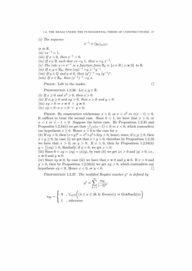
1.2. THE REALS UNDER THE FUNDAMENTAL THESIS OF CONSTRUCTIVISM 17
(i) The sequencex−1 ≡ (yn)n∈N+
is in R.(ii) xx−1 = 1.(iii) If x > 0, then x−1 > 0.(iv) If s ∈ R such that xs =R 1, then s =R x
−1.(v) The rule x 7→ x−1 is a function from R0 ≡ {x ∈ R | x on 0} to R.(vi) If x, y ∈ R0, then (xy)−1 =R x
−1y−1.(vii) If q ∈ Q and q 6= 0, then (q∗)−1 =R (q−1)∗.(viii) If x ∈ R0, then (x−1)−1 =R x.
Proof. Left to the reader. �
Proposition 1.2.36. Let x, y ∈ R.
(i) If x ≥ 0 and x2 > 0, then x > 0.(ii) If x, y ≥ 0 and xy > 0, then x > 0 and y > 0.(iii) xy > 0⇒ x on 0 ∧ y on 0.(iv) xy < 0⇒ x < 0 ∨ y < 0.
Proof. By constructive trichotomy x > 0, or x < x2 ⇔ x(x − 1) > 0.It suffices to treat the second case. Since 0 < 1, we have that x > 0, orx < 1 ⇔ x − 1 < 0. Suppose the latter case. By Proposition 1.2.35 andPropositin 1.2.34(i) we get that 1
x−1x(x−1) < 0⇔ x < 0, which contradictsour hypothesis x ≥ 0. Hence x > 0 is the case for x.(ii) If xy > 0, then (x+y)2 = x2+y2+2xy > 0, hence, since, if x, y ≥ 0, thenx+ y ≥ 0, by case (i) we get that x+ y > 0, therefore by Proposition 1.2.16we have that x > 0, or y > 0. If x > 0, then by Proposition 1.2.34(ii)y = 1
x(xy) > 0, Similarly, if y > 0, we get x > 0.(iii) Since 0 < xy = |xy| = |x||y|, by case (ii) we get |x| > 0 and |y| > 0, i.e.,x on 0 and y on 0.(iv) Since xy on 0, by case (iii) we have that x on 0 and y on 0. If x > 0 andy > 0, then by Proposition 1.2.34(ii) we get xy > 0, which contradicts ourhypothesis xy < 0. Hence x < 0, or y < 0. �
Proposition 1.2.37. The modified Royden number %∗ is defined by
%∗ ≡∞∑k=1
a2k
(−2)k,
a2k =
0 , ∀n∈N(
(4 ≤ n ≤ 2k & Even(n))⇒ Goldbach(n)
)1 , otherwise

18 1. CONSTRUCTIVE MATHEMATICS AND CLASSICAL MATHEMATICS
(i) %∗ ∈ R.(ii) If there is a proof of the disjunction
%∗ ≥ 0 ∨ %∗ ≤ 0,
then the Goldbach conjecture is decided.
Proof. (i) We work as in the proof of Proposition 1.2.7.(ii) We use the fact that, if l ∈ N+ is the first index such that a2l = 1, then
%∗ =∞∑k=l
1
(−2)k=
1
(−2)l
(1− 1
2+
1
22− 1
23+
1
24− 1
25+ . . .
)and the sign of %∗ is determined by l i.e., if l is odd, or even. �
Corollary 1.2.38. Consider the following equation (E):
x(x− %∗) = 0.
(i) The real number 0 ∧ %∗ is a solution of (E).(ii) If there is a proof of the disjunction
(0 ∧ %∗) = 0 ∨ (0 ∧ %∗) = %∗,
then the Goldbach conjecture is decided.(iii) If there is a proof of the implication
x(x− %∗) = 0⇒ (x = 0 ∨ x = %∗),
then the Goldbach conjecture is decided.
Proof. (i) Let (0 ∧ %∗)(0 ∧ %∗ − %∗) > 0. By Proposition 1.2.36(iii)we have that (0 ∧ %∗) on 0, or (0 ∧ %∗ − %∗) on 0. In the first case we get0 ≥ (0 ∧ %∗) > 0, which is a contradiction, or 0 ∧ %∗ < 0. Since 0 ∧ %∗ ≡−(−0 ∨ −%∗) = −(0 ∨ −%∗), we have that 0 ∧ %∗ < 0 ⇔ −(0 ∨ −%∗) < 0 ⇔(0 ∨ −%∗) > 0, therefore by Proposition 1.2.23(ii) we get (0 ∨ −%∗) = −%∗.Hence, 0 ∧ %∗ = −(−%∗) = %∗, and the hypothesis %∗ < 0 decides, accordingto Proposition 1.2.37(ii), the Goldbach conjecture. Hence, (0 ∧ %∗)(0 ∧ %∗ −%∗) ≤ 0.
If (0∧%∗)(0∧%∗−%∗) < 0, then by Proposition 1.2.36(iv) either 0∧%∗ < 0,or (0 ∧ %∗ − %∗) < 0. In the first case we work exactly as in the previouscase. In the second case we get 0 ∧ %∗ < %∗, and similarly we conclude that0 = 0 ∧ %∗ < %∗, hence by Proposition 1.2.37(ii) the Goldbach conjecture isdecided. Hence, (0 ∧ %∗)(0 ∧ %∗ − %∗) ≥ 0.(ii) If there is a proof of (0 ∧ %∗) = 0, then %∗ ≥ 0. If there is a proof of(0 ∧ %∗) = %∗, then %∗ ≤ 0.(iii) In this case (0 ∧ %∗) = 0 ∨ (0 ∧ %∗) = %∗, and we use (ii). �

1.3. THE TRICHOTOMY OF ALGEBRAIC NUMBERS 19
Consequently, the classical property of an integral domain
xy = 0⇒ (x = 0 ∨ y = 0)
cannot be accepted constructively for the real numbers. It is easy to showthough, that the following implication holds:
x2 = 0⇒ x = 0.
1.3. The trichotomy of algebraic numbers
Definition 1.3.1. A function f : R → R is called continuous, if forevery n ∈ N+ there is a function ωf,n : R+ → R+
0 < ε 7→ ωf,n(ε) > 0,
which is called the modulus of continuity of f on the closed interval [−n, n],and satisfies
|x− y| < ωf,n(ε)⇒ |f(x)− f(y)| ≤ ε,for every ε > 0, and x, y ∈ [−n, n]. We denote by B(R) the set of continuousfunctions from R to R.
Lemma 1.3.2. If x, y ∈ R, there is n ∈ N+ such that x, y ∈ [−n, n].
Proof. By Lemma 1.2.32 we have that x − xm ≤ 1m , hence x ≤ xm +
1m ≤ N , for some N ∈ N+. Similarly −x ≤ M ⇔ x ≥ −M , for someM ∈ N+. If k ≡ max{N,M}, then x ∈ [−k, k]. Similarly, there is l ∈ N+
such that y ∈ [−l, l]. Take n ≡ max{k, l}. �
Proposition 1.3.3. If f : R→ R is continuous and x, y ∈ R, then
f(x) on f(y)⇒ x on y.
Proof. By Lemma 1.3.2 there is n ∈ N+ such that x, y ∈ [−n, n]. Let0 < ε ≡ |f(x)−f(y)|. Suppose that |x−y| < ωf,n( ε2). Hence, |f(x)−f(y)| ≤ε2 , which contradicts our hypothesis. So, |x− y| ≥ ωf,n( ε2) > 0. �
Proposition 1.3.4. Let f, g ∈ B(R) and λ ∈ R.
(i) f + g ∈ B(R).(ii) λf ∈ B(R).(iii) f2 ∈ B(R).(iv) f · g ∈ B(R).
Proof. Exercise. For the proof of (iii) use without proof the fact thatif f ∈ B(R), then its restriction f|[−n,n] to [−n, n] is bounded i.e.,
∃Mn∈N+∀x∈[−n,n](|f(x)| ≤Mn).
�

20 1. CONSTRUCTIVE MATHEMATICS AND CLASSICAL MATHEMATICS
Definition 1.3.5. If p ∈ Q, then p : R → R denotes the constantfunction on R with value p. The set of polynomials with rational coefficientsQ[x] is defined by
Q[x] =⋃n∈N
Qn[x],
Q0[x] ≡ {p | p ∈ Q},
Qn[x] ≡{f ∈ F(R,R) | ∃p0,...,pn−1∈Q∃pn∈Q\{0}∀x∈R
(f(x) ≡
n∑i=0
pixi
)},
if n ∈ N+. If f ∈ Qn[x], where n > 0, then n = deg(f) is the degree of f . Iff ≡
∑ni=0 pix
i ∈ Q[x], we say that f is non-constant, if f ∈ Qn[x], for somen ∈ N+, and the derivative f ′ of f is the polynomial
f ′ ≡n∑i=1
ipixi−1.
A non-constant polynomial f ≡∑n
i=0 pixi is called monic, if pn = 1, Let
Q∗[x] ≡ Q[x] \ {0}. The set of algebraic real numbers A is defined by
A ≡ {x ∈ R | ∃f∈Q∗[x](f(x) = 0)}.
Clearly, Q ⊂ A, and if f(x) = 0, for some f ∈ Q∗[x], then f is non-constant. With the use of the Euclidean division algorithm one can showthat if f, g ∈ Q[x], such that their greatest common divisor (f, g) is 1,or, in other words, if f, g are relatively prime, there exist s, t ∈ Q[x] withsf + tg = 1.
Corollary 1.3.6. A polynomial f(x) in Q[x] is in B(R).
Proof. Exercise. Note that one can prove this without using Proposi-tion 1.3.4(iii). �
Lemma 1.3.7. Let x0 ∈ R, and f, g ∈ Q[x] such that (f, g) = 1. Then
f(x0)g(x0) = 0⇒ (f(x0) = 0 ∨ g(x0) = 0).
Proof. Let s, t ∈ Q[x] such that sf + tg = 1. Hence, s(x0)f(x0) +t(x0)g(x0) = 1, and
s(x0)f(x0) + t(x0)g(x0) > 0,
which by Proposition 1.2.16 implies
s(x0)f(x0) > 0 ∨ t(x0)g(x0) > 0.

1.3. THE TRICHOTOMY OF ALGEBRAIC NUMBERS 21
Suppose that s(x0)f(x0) > 0. Since
0 = s(x0)(f(x0)g(x0)
)=(s(x0)f(x0)
)g(x0),
we conclude that g(x0) = 0. Similarly, if we suppose that t(x0)g(x0) > 0,we conclude that f(x0) = 0. �
Lemma 1.3.8. If S = {f1, . . . , fn} is a finite set of monic polynomialsin Q[x], there is a finite set T = {g1, . . . , gm} of monic polynomials in Q[x]such that:
(i) If gi, gj ∈ T , thengi = gj ∨ (gi, gj) = 1.
(ii) If fk ∈ S, there are gi1 . . . , gil ∈ T such that for every x ∈ R:
fk(x) ≡il∏
j=i1
gj(x).
Proof. Left to the reader. �
E.g., if S1 = {x2, x3}, then T1 = {x}, and if S2 = {x2−4, (x−2)3}, thenT2 = {x − 2, x + 2}. Note that if S = {f} and f has a proper factor, thenthe degree of the elements of T is smaller than deg(f).
Lemma 1.3.9. Let g ∈ Q[x] a non-constant polynomial. There aref1, . . . , fr ∈ Q[x], for some r ∈ N+, and m1, . . . ,mr ∈ N+ such that:
(i) (fi, f′i) = 1, for every 1 ≤ i ≤ r.
(ii) (fmii , fmjj ) = 1, for every 1 ≤ i 6= j ≤ r.
(iii) For every x ∈ R we have that
g(x) =
r∏i=1
fmii (x).
Proof. Without loss of generality let g be monic. If deg(g) = 1, theng(x) = x + p0, for some p0 ∈ Q. Hence, (g, g′) = 1, and we take r = 1,f1 = g and m1 = 1. If deg(g) > 1, we compute (g, g′). If (g, g′) = 1, wework as in the previous case. If not, then (g, g′) is a proper factor of g,hence by Lemma 1.3.8 g is the product of monic polynomials h1, . . . , hmwith degree smaller than deg(g), which are pairwise relatively prime. Byinductive hypothesis we write them such that (i)-(iii) are satisfied, and thenthe required writing of g follows, since if (hi, hj) = 1 and
hi =s∏
ρ=1
ukρρ , hj =
t∏σ=1
wlσσ ,

22 1. CONSTRUCTIVE MATHEMATICS AND CLASSICAL MATHEMATICS
then (ukρρ , wlσσ ) = 1, for every ρ, σ. �
Theorem 1.3.10 (Julian, Mines, Richman). If a, b ∈ A, then
a < b ∨ a = b ∨ a > b.
Proof. Without loss of generality we can take monic polynomials g, hin Q[x] such that g(a) = 0 = h(b). If f = gh, then f is a monic polynomialin Q[x] such that
f(a) = 0 = f(b).
Since g, h are non-constant, f is also non-constant, hence by Lemma 1.3.9there are f1, . . . , fr ∈ Q[x] and m1, . . . ,mr ∈ N+ such that:(i) (fi, f
′i) = 1, for every 1 ≤ i ≤ r.
(ii) (fmii , fmjj ) = 1, for every 1 ≤ i 6= j ≤ r.
(iii) For every x ∈ R we have that
f(x) =
r∏i=1
fmii (x).
Since
f(a) =r∏i=1
fmii (a) = 0,
and because of condition (ii), by Lemma 1.3.7 we get some index i ∈{1, . . . , r} such that
fmii (a) = 0.
Similarly, we get some index j ∈ {1, . . . , r} such that
fmjj (b) = 0.
If i 6= j, and because of condition (ii), there are polynomials s(x), t(x) inQ[x] such that for every x ∈ R
s(x)fmii (x) + t(x)fmjj (x) = 1.
Hence, the equality
s(a)fmii (a) + t(a)fmjj (a) = 1
implies the equality t(a)fmjj (a) = 1, hence by Proposition 1.2.36(iii) t(a) on 0
and fmjj (a) on 0, therefore
fmjj (a) on f
mjj (b).
By Proposition 1.3.3 and the continuity of fmjj we get a on b.

1.4. NOTES 23
If i = j, then,fi(a)mi = 0 = fi(b)
mi ,
hencefi(a) = 0 = fi(b).
Using the elementary theory of Taylor series for the infinitely differentiablepolynomial functions we have that
fi(y) = (y − b)fi′(b) + (y − b)2K(y) = (y − b)[fi′(b) + (y − b)K(y)].
Hence(∗) 0 = fi(a) = (a− b)[fi′(b) + (a− b)K(a)].
Since (fi, fi′) = 1, there are k(x), l(x) in Q[x] such that
k(x)fi(x) + l(x)fi′(x) = 1,
for every x ∈ R. Since fi(b) = 0, we get fi′(b) on 0, and
0 on fi′(b) = fi
′(b) + (a− b)K(a)− (a− b)K(a)
= [fi′(b) + (a− b)K(a)] + [−(a− b)K(a)].
By the obvious generalisation of Proposition 1.2.16 we get
[fi′(b) + (a− b)K(a)] on 0 ∨ [−(a− b)K(a)] on 0,
and consequently
[fi′(b) + (a− b)K(a)] on 0 ∨ (a− b)K(a) on 0.
If [fi′(b)+(a−b)K(a)] on 0, then the equation (∗) implies a = b. If otherwise
(a− b)K(a) on 0, then by Proposition 1.2.36(iii) we get a on b. �
The classical behavior of the algebraic numbers A is anticipated from the“finite” information included in the definition of A, which makes A behavelike Q.
1.4. Notes
The fundamental thesis of constructivism is formulated in [5], an unpub-lished lecture of Bishop on which the first chapter is based. We also includesome notions and results from [6], a book of Bishop with Bridges, which hasa lot in common with Bishop’s original book [4], but it is a “different” bookin many respects.
With his remarkable book Foundations of constructive analysis ErrettBishop (1928-1983), an important analyst, wanted to revolutionize mathe-matics. Bishop’s achievement was to develop large parts of mathematicsusing intuitionistic logic without contradicting classical mathematics i.e.,
24 1. CONSTRUCTIVE MATHEMATICS AND CLASSICAL MATHEMATICS
mathematics based roughly on the principle of the excluded middle. BeforeBishop, it was the great topologist Luitzen Egbertus Jan Brouwer (1881-1966) who used intuitionistic logic in his intuitionistic mathematics, with-out avoiding though contradicting with classical mathematics. AlthoughBishop’s work didn’t influence the every day mathematician, it had an enor-mous impact on mathematical logic and formal studies on the foundationsof mathematics (see e.g., [2], for the influence of Bishop’s book in the logicalstudies of the 70’s and the 80’s). Today, the influence of Bishop’s paradigmis evident in theoretical computer science and especially in the current use oftype theory in Voevodsky’s univalent foundations of mathematics (see [23]).
One of the formal systems of the 70’s that was motivated a lot fromBishop’s book was Martin-Lof’s type theory (see [19] and [20]). A formalversion, or an implementation, of FTC-N in Martin-Lof’s type theory is thecanonicity property of the type of natural numbers, according to which everyclosed term of type N is reduced (simplified) to a numeral.
The definition of the equality =X between the elements of a set X isspecific to each set X and an essential part of the definition of X itself.This is a fundamental idea of Bishop’s set theory, which is in contrast to thestandard, “global” set-theoretic equality, and it is implemented in Martin-Lof’s type theory through the identity type x =A y.
The set-theoretical definition of a function f : X → Y is that f ⊆ X×Ysuch that (x, y) ∈ f and (x, z) ∈ f implies y = z, for every x ∈ X and y, z ∈Y . There are many reasons not to consider this definition of the conceptof function, since it does not reveal the dynamic character of the concept(see [12], section 2.1) In Bishop’s approach to constructive mathematics, andin many formalizations of Bishop’s constructive mathematics the notion offunction, or a rule, is taken as primitive, not reduced to some other concept,such the concept of set.
The definition of a real number, Definition 1.2.1, differs from the classi-cal one, as classically a real number is the equivalence class of the reals, asdefined here, with respect to the equivalence relation of their equality. Theavoidance of equivalence classes is a central feature of Bishop-style construc-tive mathematics.
The definition of x ≤ 0 is not given through the negation of x > 0,but it is defined positively in Definition 1.2.12. Since negation does notbehave constructively as in the classical setting, negatively defined conceptsare avoided when a positive formulation of them can be given.
In classical mathematics one finds important theorems in disjunctiveform for which no method is known (yet) that decides which disjunct is the

1.4. NOTES 25
case. E.g., Jensen proved in the early 70’s that the universe of sets V iseither “very close” to Godel’s constructible universe L, which is an innermodel of Zermelo-Fraenkel axiomatic set theory ZF in which the axiom ofchoice and the generalised continuum hypothesis are true in it, or “very far”from it.
Theorem 1.4.1. Exactly one of the following hold:
(i) Every singular cardinal γ is singular in L, and (γ+)L = γ+.(ii) Every uncountable cardinal is inaccessible in L.
Note that the proof of this theorem cannot specify which one of the twocases holds. The existence of large cardinals implies (ii), but this existenceis unprovable in ZFC, which is ZF with the axiom of choice. A similardichotomy for the inner model HOD was proved by Woodin a few yearsago. Assuming the existence of an extendible cardinal, the first alternativeof Woodin’s dichotomy implies that HOD is close to V , and the second thatHOD is far from V . At the moment there is no evidence which one of thetwo alternatives is the right one, a fact with important consequences for thefuture of set theory (see [1]).
Hence, a proof of the impossibility of (not A) and (not B) is not generallya constructive proof of A∨B (Definition 1.2.15), since such a proof does notalways imply a finite process that determines which one of the two disjunctsis the case.
Definitions 1.1.5, 1.2.3, and 1.2.15 constitute the so-called Brouwer-Heyting-Kolmogorov interpretation of logical connectives and quantifiers.
The definition of a continuous function (Definition 1.3.1) is one of themajor keys in Bishop’s development of constructive analysis. By “replacing”pointwise continuity of a real-valued function on R with uniform continuityon the compact intervals [−n, n] of R he managed to avoid clashing withclassical analysis.
Section 1.3 draws from the paper [17] of Julian, Mines and Richman.For a development of Bishop-style constructive algebra see [21].

CHAPTER 2
Constructive Logic and Classical Logic
2.1. First-order languages
Definition 2.1.1. Let Var = { vi | i ∈ N } be a fixed countably infiniteset of variables. We also denote the elements of Var by x, y, z, etc. . LetL = {→,∧,∨,∀,∃, (, ), , }, where each element of L is called a logical sym-bol. A first-order language over Var and L is a pair L = (Rel, Fun), whereVar, L, Rel, Fun are pairwise disjoint sets such that
Rel =⋃n∈N
Rel(n),
where for every n ∈ N, Rel(n) is a (possible empty) set of n-ary relation
symbols (or predicate symbols). Moreover, Rel(n) ∩ Rel(m) = ∅, for everyn 6= m. A 0-ary relation symbol is called a propositional symbol . Thesymbol ⊥ (read “falsum”) is required as a fixed propositional symbol (i.e.,
Rel(0) is inhabited by ⊥). The language will not, unless stated otherwise,contain the equality symbol =, which is a 2-ary relation symbol. Moreover,
Fun =⋃n∈N
Fun(n),
where for every n ∈ N, Fun(n) is a (possible empty) set of n-ary function
symbols. Moreover, Fun(n) ∩ Fun(m) = ∅, for every n 6= m. A 0-ary functionsymbol is called constant , and we define
Const ≡ Fun(0).
The pair (Rel, Fun) is called the signature of L.
Note that this definition uses the notion of set, therefore it is given withinsome theory of sets, which is the meta-theory of our theory of first-orderlanguages. Here we choose as meta-theory the classical theory of sets. Allproofs of properties of first-order languages are given within set-theory. Onecould use as meta-theory the constructive theory of sets that was roughly
27

28 2. CONSTRUCTIVE LOGIC AND CLASSICAL LOGIC
introduced in the previous chapter, and also use constructive arguments inthe related proofs.
If our formal language includes one more fixed countably infinite set ofvariables VAR = {Vi | i ∈ N}, where Vi is a variable of another sort, e.g., aset-variable, then one could define the notion of a second-order language ina similar fashion.
The first-order language of arithmetic has as signature the pair ({⊥,=}, {0, S,+, ·}), which is written for simplicity as (⊥,=, 0, S,+, ·) , such that
0 ∈ Const, S ∈ Fun(1), and +, · ∈ Fun(2). The first-order language of settheory has signature the pair ({⊥,=,∈}, ∅)}), which is written for simplicity
as (⊥,=,∈), such that ∈ is in Rel(2).Next, the terms TermL of a first-order language L are inductively defined.
For simplicity we omit the subscript L.
Definition 2.1.2. The terms Term of a first-order language L are definedby the following inductive rules:
x ∈ Var
x ∈ Term,
c ∈ Const
c ∈ Term,
n ∈ N+, t1, . . . , tn ∈ Term, f ∈ Fun(n)
f(t1, . . . , tn) ∈ Term.
In words, every variable is a term, every constant is a term, and ift1, . . . , tn are terms and f is an n-ary function symbol with n ≥ 1, thenf(t1, . . . , tn) is a term. If r, s are terms and ◦ is a binary function symbol,we usually write (r ◦ s) instead of ◦(r, s). E.g.,
0, S(0), S(S(0)), (S(0) + S(S(0)))
are terms of the language of arithmetic.As in the case of the inductive definition of N, we associate to Defini-
tion 2.1.2 the following induction principle:
∀x∈Var(P (x)),
∀c∈Const(P (c)),
∀n∈N+∀t1,...,tn∈Term∀f∈Fun(n)((P (t1) ∧ . . . ∧ P (tn))⇒ P (f(t1, . . . , tn))
∀t∈Term(P (t)),
where P (t) is any property of our meta-language that concerns the set ofterms. E.g., P (t) could be “the number of left parentheses, (, occurring int is equal to the number of right parentheses, ), occurring in t”. We needof course, to express this property in mathematical terms. As in the case

2.1. FIRST-ORDER LANGUAGES 29
of the induction principle for natural numbers, the induction principle forTerm expresses that Term is the least set satisfying its defining rules.
As one can show for N that if X is a set, x0 ∈ X and g : X → X, thereis a unique function f : N→ X such that
f(0) ≡ x0,
f(S(n)) ≡ g(f(n)),
for every n ∈ N, the following recursion theorem holds for Term.
Proposition 2.1.3 (Recursion theorem for Term). Let X be a set. Ifthere are functions
FVar : Var→ X,
FConst : Const→ X,
Ff,n : Xn → X,
for every f ∈ Fun(n) and n ∈ N+, then there is a unique function
F : Term→ X
such that, for every n ∈ N+, t1, . . . , tn ∈ Term, and f ∈ Fun(n),
F (x) ≡ FVar(x), x ∈ Var,
F (c) ≡ FConst(c), c ∈ Const,
F (f(t1, . . . , tn)) ≡ Ff,n(F (t1), . . . , F (tn)).
Proof. Let F ⊆ Term×X defined as follows:
F ≡ {(ui, FVar(ui)) | ui ∈ Var} ∪ {(c, FConst(c)) | c ∈ Const}∪{
(f(t1, . . . , tn), Ff,n(x1, . . . , xn) | t1, . . . , tn ∈ Term,
(t1, x1), . . . , (tn, xn) ∈ F, f ∈ Fun(n), n ∈ N+}.
Using the induction principle for Term we show that F is a function i.e.,
∀t∈Term(∀x,y∈X((t, x) ∈ F ∧ (t, y) ∈ F ⇒ x = y)
).
If t ≡ ui, for some i ∈ N, then (ui, x) ∈ F ⇔ x = FVar(ui) and (ui, y) ∈F ⇔ y = FVar(ui). Since FVar is a function, we get x = y. If t ≡ c, for somec ∈ Const, then (c, x) ∈ F ⇔ c = FConst(c) and (c, y) ∈ F ⇔ y = FConst(c).Since FConst is a function, we get x = y. If t ≡ f(t1, . . . , tn), for some
t1, . . . , tn ∈ Term and f ∈ Fun(n), then
(f(t1, . . . , tn), x) ∈ F ⇔ x = Ff,n(x1, . . . , xn)∧(t1, x1) ∈ F ∧ . . . (tn, xn) ∈ F,for some x1, . . . , xn ∈ X. Similarly,
(f(t1, . . . , tn), y) ∈ F ⇔ y = Ff,n(y1, . . . , yn) ∧ (t1, y1) ∈ F ∧ . . . (tn, yn) ∈ F,

30 2. CONSTRUCTIVE LOGIC AND CLASSICAL LOGIC
for some y1, . . . , yn ∈ X. By the inductive hypothesis on t1, . . . , tn we get
x1 = y1 ∧ . . . ∧ xn = yn,
and since Ff,n is a function, from
((x1, . . . , xn), x) ∈ Ff,n ∧ ((x1, . . . , xn), y) ∈ Ff,nwe get x = y. Using the induction principle for Term we get Term ⊆ dom(F )i.e.,
∀t∈Term(t ∈ dom(F )
).
If t ≡ ui, for some i ∈ N, then (ui, FVar(x)) ∈ F , therefore ui ∈ dom(F ). Ift ≡ c, for some c ∈ Const, then (c, FConst(c)) ∈ F , therefore c ∈ dom(F ).
If t ≡ f(t1, . . . , tn), for some t1, . . . , tn ∈ Term and f ∈ Fun(n), such thatt1, . . . , tn ∈ dom(F ). Hence, there are x1, . . . , xn ∈ such that (t1, x1) ∈F ∧ . . . (tn, xn) ∈ F . By the definition of F we get
(f(t1, . . . , tn), Ff,n(x1, . . . , xn) ∈ F,hence f(t1, . . . , tn) ∈ dom(F ). The uniqueness of F is also shown again withthe use of the induction principle for Term. If G : Term → X satisfies thedefining properties of F , it is easy to show now that
∀t∈Term(F (t) = G(t)
).
�
Using the recursion theorem for Term one can define e.g., the functionPleft : Term → N such that Pleft(t) is the number of left parentheses oc-curring in t ∈ Term. It suffice to define it on the variables, the constants,and the complex terms f(t1, . . . , tn) supposing that Pleft is defined on theterms t1, . . . , tn. Namely, we define
Pleft(ui) ≡ 0,
Pleft(c) ≡ 0,
Pleft(f(t1, . . . , tn)) ≡ 1 +
n∑i=1
Pleft(ti).
Here we used the recursion theorem for Term with respect the functions
FVar(x) ≡ 0 ≡ FConst(c),
Ff,n(x1, . . . , xn) ≡ 1 +
n∑i=1
xi.
Similarly, one defines the function Pright : Term → N such that Pright(t) isthe number of right parentheses occurring in t ∈ Term.

2.1. FIRST-ORDER LANGUAGES 31
Proposition 2.1.4. ∀t∈Term(Pleft(t) = Pright(t)
).
Proof. Exercise. �
Definition 2.1.5. The formulas Form of a first-order language L aredefined by the following inductive rules:
n ∈ N, t1, . . . , tn ∈ Term, R ∈ Rel(n)
R(t1, . . . , tn) ∈ Form,
A,B ∈ Form
(A→ B), (A ∧B), (A ∨B) ∈ Form,
A ∈ Form, x ∈ Var
∀xA, ∃xA ∈ Form.
The formulas of the form R(t1, . . . , tn) are called prime formulas, or atomicformulas, or just atoms. If r, s are terms and ∼ is a binary relation symbol,we also write (r ∼ s) for the prime formula ∼ (r, s). Since ⊥ ∈ Rel(0), weget ⊥ ∈ Form. The negation ¬A of a formula A is defined as the formula
¬A ≡ A→ ⊥.The formulas generated by the prime formulas are called complex, or non-atomic formulas. Usually, we denote (A�B) by A�B, where � ∈ {→,∧,∨}.We also define
A→ B → C ≡ A→ (B → C).
These are some examples of formulas:
(⊥ → ⊥), ∀x(⊥ → ⊥), ∃x(R(x) ∨ S(x)).
To the Definition 2.1.5 we associate the following induction principle:
∀n∈N∀t1,...,tn∈Term∀R∈Rel(n)(P (R(t1, . . . , tn))),
∀A,B∈Form(P (A) ∧ P (B)⇒
(P (A→ B) ∧ P (A ∧B) ∧ P (A ∨B)
)),
∀A∈Form∀x∈Var(P (A)⇒ P (∀xA) ∧ P (∃xA)
)∀A∈Form(P (A))
,
where P (A) is any property of our meta-language that concerns the set offormulas. E.g., P (A) could be “the number of left parentheses occurring inA is equal to the number of right parentheses occurring in A”. The inductionprinciple for Form expresses that Form is the least set satisfying its definingrules.
Note that the induction principle for Form consists of formulas of ourmeta-theory, where the same quantifiers and logical symbols, except fromthe meta-theoretic implication symbol ⇒, are used. Since the variables

32 2. CONSTRUCTIVE LOGIC AND CLASSICAL LOGIC
occurring in these meta-theoretic formulas are different from Var, it is easyto understand from the context the difference between the formulas in Form
and the formulas in our meta-theory. As in the case of terms, we have arecursion theorem for Form.
Proposition 2.1.6 (Recursion theorem for Form). Let X be a set. Ifthere are functions
FRel :{R(t1, . . . , tn) | R ∈ Rel(n), t1, . . . , tn ∈ Term, n ∈ N
}→ X
F→, F∧, F∨ : X ×X → X,
F∀,x, F∃,x : X → X,
for every x ∈ Var, then there is a unique function
F : Form→ X
such that
F (R(t1, . . . , tn)) ≡ FRel(R(t1, . . . , tn)),
F (A→ B) ≡ F→(F (A), F (B)),
F (A ∧B) ≡ F∧(F (A), F (B)),
F (A ∨B) ≡ F∨(F (A), F (B)),
F (∀xA) ≡ F∀,x(F (A)),
F (∃xA) ≡ F∃,x(F (A)).
Proof. We work similarly to the proof of Proposition 2.1.3. �
Definition 2.1.7. The function |.| : Form → N determines the height|A| of a formula A and it is defined by the clauses
|P | ≡ 0, P is atomic,
|A�B| ≡ max{|A|, |B|}+ 1, � ∈ {→,∧,∨},|4xA| ≡ |A|+ 1, 4 ∈ {∀,∃}.
In the previous definition we used the recursion theorem for Form withrespect the following functions:
FRel(P ) ≡ 0,
F�(a, b) ≡ max{a, b}+ 1,
F4,x(a) ≡ a+ 1.

2.1. FIRST-ORDER LANGUAGES 33
Definition 2.1.8. The function ||.|| : Form → N determines the length||A|| of a formula A and it is defined by the clauses ||.|| : Form → N by thefollowing conditions:
||P || ≡ 1, P is atomic,
||A � B|| ≡ ||A||+ ||B||, {→,∧,∨},||4xA|| = 1 + ||A||, 4 ∈ {∀,∃}.
Proposition 2.1.9. ∀A∈Form(||A||+ 1 ≤ 2|A|+1).
Proof. Exercise. �
Definition 2.1.10. The function FVTerm : Term → Pfin(Var), wherePfin(X) denotes the finite subsets of some set X, expresses the set of (free)variables occurring in a term and it is defined by the clauses
FVTerm(x) ≡ {x},FVTerm(c) ≡ ∅,
FVTerm(f(t1, . . . , tn)) ≡n⋃i=1
FVTerm(ti).
The function FVForm : Form → Pfin(Var) expresses the set of free variablesoccurring in a formula and it is defined by the clauses
FVForm(R) = ∅, R ∈ Rel(0),
FVForm(R(t1, . . . , tn)) ≡n⋃i=1
FVTerm(ti), R ∈ Rel(n), n ∈ N+,
FVForm(A�B) ≡ FVForm(A) ∪ FVForm(B),
FVForm(4xA) ≡ FVForm(A) \ {x}.If FV(A) = ∅, we call A a sentence, or a closed formula.
According to Definition 2.1.10, a variable y is free in a prime formula A,if just occurs in A, it is free in A�B, if it is free in A or free in B, and it isfree in 4xA, if it is free in A and y 6= x. E.g.,
∀y(R(y)→ S(y)), ∀y(R(y)→ ∀zS(z))
are sentences, and y is free in
(∀y(R(y))→ S(y).
Definition 2.1.11. W(L) is the set of finite lists of symbols from theset Var ∪ L ∪ Rel ∪ Fun. The set W(L) can be defined inductively, and itselements are called words of L.

34 2. CONSTRUCTIVE LOGIC AND CLASSICAL LOGIC
Note that Term, Form ⊂ W(L), and fR ∧ g(⊥, u8 is a word which isneither in Term nor in Form.
Definition 2.1.12. If s ∈ Term and x ∈ Var are fixed, the function
Subs/x : Term→W(L)
t 7→ t[x := s] ≡ Subs/x(t),
determines the word generated by substituting x from s in t and it is definedby the clauses
vi[x := s] ≡{s , x ≡ vivi , otherwise,
c[x := s] ≡ c,f(t1, . . . , tn)[x := s] ≡ f(t1[x := s], . . . , tn[x := s]).
Proposition 2.1.13. ∀t∈Term(t[x := s] ∈ Term).
Proof. Exercise. �
Proposition 2.1.14. ∀t∈Term(x /∈ FV(t)⇒ t[x := s] ≡ t).
Proof. We use induction on Term. If t ≡ vi, for some vi ∈ Var, thenx /∈ FV(vi) ↔ x /∈ {vi} ⇔ x 6= vi, hence vi[x := s] ≡ vi. If t ≡ c, forsome c ∈ Const, then x /∈ FV(c) ↔ x /∈ ∅, which is always the case. By
definition we get c[x := s] ≡ c. If t ≡ f(t1, . . . , tn), for some f ∈ Fun(n) andt1, . . . , tn ∈ Term, then x /∈ FV(f(t1, . . . , tn)) ↔ x /∈ FV(ti), for every i ∈{1, . . . , n}. By the inductive hypothesis on t1, . . . , tn we get ti[x := s] ≡ ti,for every i ∈ {1, . . . , n}. Hence,
f(t1, . . . , tn)[x := s] ≡ f(t1[x := s], . . . , tn[x := s]) ≡ f(t1, . . . , tn).
�
If we consider the formula
A ≡ ∃y(¬(y = x)),
then the possible substitution of x from y would generate the formula
∃y(¬(y = y)),
which cannot be true in any “interpretation” of these symbols i.e., when yranges over some collection of objects and = is the equality of the objects inthis collection. Hence, we need to be careful with substitution on semantical(see chapter 4), rather than syntactical, grounds. Note also that x is free inA, and if it is substituted by y, then y is bound in A. This is often called a“capture”, and we want to avoid them.

2.1. FIRST-ORDER LANGUAGES 35
Definition 2.1.15. Let s ∈ Term, such that FV(s) = {y1, . . . , ym}, andx ∈ Var. If 2 ≡ {0, 1}, the function
Frees,x : Form→ 2
expresses when “the variable x is substitutable (free to be substituted) froms in some formula” i.e., if Frees,x(A) = 1, then x is substitutable from sin A, and if Frees,x(A) = 0, then x is not substitutable from s in A. Thefunction Frees,x is defined by the clauses
Frees,x(P ) ≡ 1, P is atomic,
Frees,x(A�B) ≡ Frees,x(A) · Frees,x(B),
Frees,x(4yA) ≡
0 , x = y ∨ [x 6= y ∧ y ∈ {y1, . . . , ym}]1, , x 6= y ∧ x /∈ FV(A) \ {y}Frees,x(A) , x 6= y ∧ y /∈ {y1, . . . , ym} ∧ x ∈ FV(A).
According to Definition 2.1.15, x is substitutable from s in a primeformula, since there are no quantifiers in it that can generate a capture.It is substitutable in A�B, if it is substitutable both in A and B. In thecase of an ∃, or ∀-formula 4yA, if x is not free in A (which is equivalent tox 6= y ∧ x /∈ FV(A) \ {y}), then we set Frees,x(4yA) ≡ 1, since no captureis possible to be generated.
If A ≡ ∃y(¬(y = x)), then, according to Definition 2.1.15, we get
Freey,x(∃y(¬(y = x))
)= 0.
If x, y, z are distinct variables, it is easy to see that
Freez,x(R(x)) = 1,
Freez,x(∀zR(x)
)= 0,
Freef(x,z),x
(∀yS(x, y)
)= 1,
Freef(x,z),x
(∃z∀y(S(x, y)⇒ R(x))
)= 0.
From now on, when we define a function on Form that is based on afunction on Term, as in the case of FVForm and FVTerm, we omit the subscriptsand we understand from the context their domain of definition.
Definition 2.1.16. If s ∈ Term and x ∈ Var are fixed, the function
Subs/x : Form→W(L)
A 7→ A[x := s] ≡ Subs/x(A),
36 2. CONSTRUCTIVE LOGIC AND CLASSICAL LOGIC
determines the word generated by substituting x from s in A, and it isdefined as follows:
if Frees,x(A) = 0, then A[x := s] ≡ A,while if Frees,x(A) = 1, we use the following clauses:
R[x := s] ≡ R, R ∈ Rel(0),
R(t1, . . . , tn)[x := s] ≡ R(t1[x := s], . . . , tn[x := s]), R ∈ Rel(n), n ∈ N+,
(A�B)[x := s] ≡ (A[x := s]�B[x := s]),
(4yA)[x := s] ≡ 4y(A[x := s]).
Often, we write for simplicity A(s) instead of A[x := s].
Note that if Frees,x(A�B) = 1, then Frees,x(A) = Frees,x(B) = 1, andif Frees,x(4yA) = 1, then Frees,x(A) = 1.
Proposition 2.1.17. ∀A∈Form(A[x := s] ∈ Form).
Proof. Exercise. �
Proposition 2.1.18. ∀A∈Form(x /∈ FV(A)⇒ A[x := s] ≡ A).
Proof. We use induction on Form. If A ≡ R, for some R ∈ Rel(0), thenx /∈ FV(R)↔ x /∈ ∅, which is always the case. Since Frees,x(R) = 1, by de-finition of substitution we get R[x := s] ≡ R. If A ≡ R(t1, . . . , tn), for some
R ∈ Rel(n), n ∈ N+, and t1, . . . , tn ∈ Term, then x /∈ FV(R(t1, . . . , tn)) ↔x /∈
⋃ni=1 FV(ti), for every i ∈ {1, . . . , n}. By Proposition 2.1.14 we get
ti[x := s] ≡ ti, for every i ∈ {1, . . . , n}, hence, since Frees,x(R(t1, . . . , tn)) =1, we have that
R(t1, . . . , tn)[x := s] ≡ R(t1[x := s], . . . , tn[x := s]) ≡ R(t1, . . . , tn).
If our formula is of the the form A�B, then x /∈ FV(A�B)⇔ x /∈ FV(A)∪FV(B) ⇔ x /∈ FV(A) and x /∈ FV(B). If Frees,x(A�B) = 0, then we getimmediately what we want. If Frees,x(A�B) = 1, then by the inductivehypothesis on A,B we get A[x := s] ≡ A and B[x := s] ≡ B, hence byDefinition 2.1.16 we have that
(A�B)[x := s] ≡ (A[x := s]�B[x := s]) ≡ (A�B).
If our formula is of the form 4yA, then x /∈ FV(4yA) ⇔ x /∈ FV(A) \{y} ⇔ x /∈ FV(A) or x = y. If x = y, then Frees,x(4yA) = 0, hence(4yA)[x := s] ≡ 4yA. If x /∈ FV(A) \ {y} and x 6= y, then x /∈ FV(A), andby inductive hypothesis on A we get
(4yA)[x := s] ≡ 4y(A[x := s]) ≡ 4yA.

2.2. DERIVATIONS IN MINIMAL LOGIC 37
If x ∈ FV(A), and x 6= y ∧ y /∈ {y1, . . . , ym}, the required implicationfollows trivially. �
If ~x ≡ (x1, . . . , xn) is a given n-tuple of distinct variables in Var and~s ≡ (s1, . . . , sn) is a given n-tuple of terms in Term, for some n ∈ N+, wecan define similarly for every formula A the formula A[~x := ~s] generated bythe substitution of xi from si in A, for every i ∈ {1, . . . , n}.
2.2. Derivations in minimal logic
To motivate the rules for natural deduction, let us start with informalproofs of some simple logical facts. We consider the following formula
D ≡ (A→ B → C)→ (A→ B)→ A→ C,
which, according to our notational convention, is the formula
(A→ B → C)→ ((A→ B)→ (A→ C)).
First we give an informal proof of D using the Brouwer-Heyting-Kolmogorovinterpretation of → (Definition 1.1.5). According to it, a proof
p : (A→ B → C)→ ((A→ B)→ (A→ C))
is a rule that sends a supposed proof q : A→ B → C to a proof
p(q) : (A→ B)→ (A→ C),
which is a rule that sends a proof r : A→ B to a proof
p(q, r) ≡ [p(q)](r) : A→ C,
which is a rule that sends a proof s : A to a proof
p(q, r, s) ≡ {[p(q)](r)}(s) : C.
We define this proof by
p(q, r, s) ≡ q(s, r(s)).Another informal proof of D goes as follows: Assume A→ B → C. To show(A → B) → A → C, we assume A → B. To show A → C we assume A.We show C by using the third assumption twice and we have B → C by thefirst assumption, and B by the second assumption. From B → C and B weobtain C. Then we obtain A → C by cancelling the assumption on A, and(A → B) → A → C by cancelling the second assumption; and the resultfollows by cancelling the first assumption.
We consider next the formula
E ≡ ∀x(A→ B)→ A→ ∀xB, if x /∈ FV(A).

38 2. CONSTRUCTIVE LOGIC AND CLASSICAL LOGIC
First we give an informal proof of E using the Brouwer-Heyting-Kolmogorovinterpretation of →, ∀xA (Definition 1.1.5), without specifying though someset X in which the variable x ranges over. According to it, a proof
p : ∀x(A→ B)→ A→ ∀xB
is a rule that sends a supposed proof q : ∀x(A→ B) to a proof
p(q) : A→ ∀xB,
which is a rule that sends a proof r : A to some proof
p(q, r) : ∀xB.
The proof q : ∀x(A→ B) is understood as a family of proofs
q ≡(qx : A→ B
)x,
and, similarly, the required proof p(q, r) : ∀xB is a family of proofs
p(q, r) ≡([p(q, r)]x : B
)x.
We define this family of proofs by
[p(q, r)]x ≡ qx(r).
Another informal proof of E goes as follows: Assume ∀x(A→ B). To showA → ∀xB we assume A. To show ∀xB let x be arbitrary; note that wehave not made any assumptions on x. To show B we have A → B by thefirst assumption, and hence also B by the second assumption. Hence ∀xB.Hence A→ ∀xB, cancelling the second assumption. Hence E, cancelling thefirst assumption.
A characteristic feature of the second kind of informal proofs is thatassumptions are introduced and eliminated again. At any point in timeduring the proof the free or “open” assumptions are known, but as the proofprogresses, free assumptions may become cancelled or “closed” because ofthe implies-introduction rule.
We reserve the word proof for the informal level; a formal representationof a proof will be called a derivation.
An intuitive way to communicate derivations is to view them as labelledtrees each node of which denotes a rule application. The labels of the innernodes are the formulas derived as conclusions at those points, and the labelsof the leaves are formulas or terms. The labels of the nodes immediatelyabove a node k are the premises of the rule application. At the root ofthe tree we have the conclusion (or end formula) of the whole derivation.In natural deduction systems one works with assumptions at leaves of the

2.2. DERIVATIONS IN MINIMAL LOGIC 39
tree; they can be either open or closed (cancelled). Any of these assump-tions carries a marker . As markers we use assumption variables denotedu, v, w, u0, u1, . . . . The variables in Var will now often be called object vari-ables, to distinguish them from assumption variables. If at a node belowan assumption the dependency on this assumption is removed (it becomesclosed), we record this by writing down the assumption variable. Since thesame assumption may be used more than once (this was the case in the firstexample above), the assumption marked with u (written u : A) may appearmany times. Of course we insist that distinct assumption formulas musthave distinct markers.
An inner node of the tree is understood as the result of passing frompremises to the conclusion of a given rule. The label of the node then con-tains, in addition to the conclusion, also the name of the rule. In some casesthe rule binds or closes or cancels an assumption variable u (and henceremoves the dependency of all assumptions u : A thus marked). An appli-cation of the ∀-introduction rule similarly binds an object variable x (andhence removes the dependency on x). In both cases the bound assumptionor object variable is added to the label of the node.
First we have an assumption rule, allowing to write down an arbitraryformula A together with a marker u:
u : A assumption.
The other rules of natural deduction split into introduction rules (I-rules forshort) and elimination rules (E-rules) for the logical connectives which, forthe time being, are just→ and ∀. For implication→ there is an introductionrule →+ and an elimination rule →− also called modus ponens. The leftpremise A→ B in →− is called the major (or main) premise, and the rightpremise A the minor (or side) premise. Note that with an application of the→+-rule all assumptions above it marked with u : A are cancelled (whichis denoted by putting square brackets around these assumptions), and theu then gets written alongside. There may of course be other uncancelledassumptions v : A of the same formula A, which may get cancelled at a laterstage.
Definition 2.2.1. The introduction and elimination rules for implica-tion are:
[u : A]
|MB →+uA→ B
|MA→ B
| NA →−B

40 2. CONSTRUCTIVE LOGIC AND CLASSICAL LOGIC
For the universal quantifier ∀ there is an introduction rule ∀+ (againmarked, but now with the bound variable x) and an elimination rule ∀−whose right premise is the term r to be substituted. The rule ∀+x withconclusion ∀xA is subject to the following (eigen-)variable condition to avoidcapture: the derivation M of the premise A must not contain any openassumption having x as a free variable.
|MA ∀+x∀xA
|M∀xA r ∈ Term
∀−A(r)
For disjunction the introduction and elimination rules are
|MA ∨+
0A ∨B
| NB ∨+
1A ∨B
|MA ∨B
[u : A]
| NC
[v : B]
| KC ∨−u, v
C
For conjunction we have the rules
|MA
| NB ∧+
A ∧B
|MA ∧B
[u : A] [v : B]
| NC ∧− u, v
C
and for the existential quantifier we have the rules
r ∈ Term
|MA(r)
∃+∃xA
|M∃xA
[u : A]
| NB ∃−x, u (var.cond.)
B
Similar to ∀+x the rule ∃−x, u is subject to an (eigen-)variable condition:in the derivation N the variable x (i) should not occur free in the formulaof any open assumption other than u : A, and (ii) should not occur free inB. Again, in each of the elimination rules ∨−, ∧− and ∃− the left premise iscalled major (or main) premise, and the right premise is called the minor(or side) premise.
The rule ∨−u, v
|MA ∨B
[u : A]
| NC
[v : B]
| KC ∨−u, v
C

2.2. DERIVATIONS IN MINIMAL LOGIC 41
is understood as follows: given a derivation tree for A∨B and derivation treesfor C with assumption variables u : A and v : B, respectively, a derivationtree for C is formed, such that u : A and v : B are cancelled. Similarly weunderstand the rules →+u, ∧− u, v and ∃−x, u.
Definition 2.2.2. A formula A is called derivable (in minimal logic),written
` A,
if there is a derivation of A (without free assumptions) using the naturaldeduction rules of Definition 2.2.1. A formula A is called derivable fromassumptions A1, . . . , An, written
{A1, . . . , An} ` A, or simpler A1, . . . , An ` A,
if there is a derivation of A with free assumptions among A1, . . . , An. Thefollowing tree
u : A axA
is a derivation tree of a formula A from assumption A i.e., we always have
A ` A.
If Γ ⊆ Form, a formula A is called derivable from Γ, written
Γ ` A,
if A is derivable from finitely many assumptions A1, . . . , An ∈ Γ.
Note that the rules of Definition 2.2.1 are used in the presence of freeassumptions in the same way. E.g., next follows a derivation tree for C withassumption formula G:
w : G|M
A ∨B
[u : A]
| NC
[v : B]
| KC ∨−u, v
C
We now give derivations of the two example formulas D,E, treated in-formally above. Since in many cases the rule used is determined by theconclusion, we suppress in such cases the name of the rule. First we givethe derivation of D:

42 2. CONSTRUCTIVE LOGIC AND CLASSICAL LOGIC
[u : A→ B → C] [w : A]
B → C
[v : A→ B] [w : A]
BC →+wA→ C →+v
(A→ B)→ A→ C→+u
(A→ B → C)→ (A→ B)→ A→ C
Next we give the derivation of E:
[u : ∀x(A→ B)] x ∈ Var
A→ B [v : A]
B ∀+x∀xB →+vA→ ∀xB →+u∀x(A→ B)→ A→ ∀xB
Note that the variable condition is satisfied: In the derivation of B the stillopen assumption formulas are A and ∀x(A → B); by hypothesis x is notfree in A, and by Definition 2.1.10 it is also not free in ∀x(A→ B).
Proposition 2.2.3. The following formulas are derivable:(i) A→ A.(ii) A→ ¬¬A.(iii) (Brouwer) ¬¬¬A→ ¬A.
Proof. The derivation for (i) is
[u : A]ax
A →+uA→ A
The derivation for (ii) is
[v : A→ ⊥] [u : A]
⊥ →+v(A→ ⊥)→ ⊥
→+uA→ (A→ ⊥)→ ⊥
The derivation for (iii) is an exercise. �
Note that the formula DNS ≡ ¬¬A→ A, which is known as the doublenegation shift, is in general not derivable in minimal logic.

2.2. DERIVATIONS IN MINIMAL LOGIC 43
Proposition 2.2.4. The following are derivable.
(i) (A→ B)→ ¬B → ¬A,(ii) ¬(A→ B)→ ¬B,(iii) ¬¬(A→ B)→ ¬¬A→ ¬¬B,(iv) (⊥ → B)→ (¬¬A→ ¬¬B)→ ¬¬(A→ B),
(v) ¬¬∀xA→ ∀x¬¬A.
Proof. Exercise. �
Proposition 2.2.5. We consider the following formulas:
ax∨+0 ≡ A→ A ∨B,
ax∨+1 ≡ B → A ∨B,
ax∨− ≡ A ∨B → (A→ C)→ (B → C)→ C,
ax∧+ ≡ A→ B → A ∧B,ax∧− ≡ A ∧B → (A→ B → C)→ C,
ax∃+ ≡ A→ ∃xA,ax∃− ≡ ∃xA→ ∀x(A→ B)→ B (x /∈ FV(B)).
(i) The formulas ax∨+0 , ax∨
+1 and ax∨− are equivalent, as axioms, to the
rules ∨+0 , ∨+
1 and ∨−u, v over minimal logic.(ii) The formulas ax∧+ and ax∧− as axioms are equivalent, as axioms, tothe rules ∧+ and ∧− over minimal logic.(iii) The formulas ax∃+ and ax∃− are equivalent, as axioms, to the rules∃+ and ∃−x, u over minimal logic.
Proof. (i) First we show that from the axiom ax∨+0 , a derivation of
which is considered the formula itself, and a supposed derivation M of A weget the following derivation of A ∨B
A→ A ∨B|MA →−A ∨B
Similarly we show that from the formula ax∨+1 and a supposed derivation
N of A we get a derivation of A ∨ B. Next we show that from the formulaax∨− and supposed derivations M of A ∨ B, N of C with assumption A,

44 2. CONSTRUCTIVE LOGIC AND CLASSICAL LOGIC
and K of C with assumption B we get the following derivation of C
ax∨−|M
A ∨B →−(A→ C)→ (B → C)→ C
[u : A]
| NC →+uA→ C
→−(B → C)→ C
[v : B]
| KC →+uB → C
→−C
Conversely, from the rule ∨+0 we get the following derivation of ax∨+
0
[u : A]ax
A ∨+0A ∨B →+uA→ A ∨B
Similarly, from the rule ∨+1 we get a derivation of ax∨+
1 . From the elimina-tion rule for disjunction we get the following derivation of ax∨−
[u : A ∨B]ax
A ∨B[v : A→ C] [v′ : A]
C
[w : B → C] [w′ : B]
C ∨−v′, w′C →+w
(B → C)→ C→+v
(A→ C)→ (B → C)→ C→+u
A ∨B → (A→ C)→ (B → C)→ C
(ii) and (iii) Exercises. �
Note that in the above derivation of C
u : A ∨B axA ∨B
[v : A→ C] [v′ : A]
C
[w : B → C] [w′ : B]
C ∨−v′, w′C
we used the rule ∨−v′, w′ in the “extended” way described previously, wherethe assumption variable u : A∨B is still open. Of course, it will be cancelledlater in the derivation of ax∨−.
The notation B ← A means A→ B.
Proposition 2.2.6. The following formulas are derivable
(i) (A ∧B → C)↔ (A→ B → C),
(ii) (A→ B ∧ C)↔ (A→ B) ∧ (A→ C),

2.2. DERIVATIONS IN MINIMAL LOGIC 45
(iii) (A ∨B → C)↔ (A→ C) ∧ (B → C),
(iv) (A→ B ∨ C)← (A→ B) ∨ (A→ C),
(v) (∀xA→ B)← ∃x(A→ B) if x /∈ FV(B),
(vi) (A→ ∀xB)↔ ∀x(A→ B) if x /∈ FV(A),
(vii) (∃xA→ B)↔ ∀x(A→ B) if x /∈ FV(B),
(viii) (A→ ∃xB)← ∃x(A→ B) if x /∈ FV(A).
Proof. (i) - (vii) Exercise. A derivation of the final formula is
[u : ∃x(A→ B)]x ∈ Var
[w : A→ B] [v : A]
B∃xB ∃−x,w∃xB →+vA→ ∃xB →+u∃x(A→ B)→ A→ ∃xB
The variable condition for ∃− is satisfied since the variable x (i) is not freein the formula A of the open assumption v : A, and (ii) is not free in ∃xB.Of course, it is not a problem that it occurs free in A→ B. �
Proposition 2.2.7. If Γ,∆ ⊆ Form and A,B ∈ Form, the followingrules hold:
Γ ` A, Γ ⊆ ∆ext
∆ ` A
Γ ` A, ∆ ∪ {A} ` Bcut
Γ ∪∆ ` BProof. The ext-rule is an immediate consequence of the definition of
Γ ` A. Suppose next that there are C1, . . . , Cn ∈ Γ and D1, . . . , Dm ∈∆ such that C1, . . . , Cn ` A and D1, . . . , Dm, A ` B. The following is aderivation of B from assumptions in Γ ∪∆:
u1 : D1 . . . um : Dm [u : A]
|MB →+uA→ B
w1 : C1 . . . wn : Cn| NA →−B
�

46 2. CONSTRUCTIVE LOGIC AND CLASSICAL LOGIC
The following rules are special cases of the cut-rule for Γ = ∆ andΓ = ∆ = ∅, respectively.
Γ ` A, Γ ∪ {A} ` BΓ ` B
` A, A ` B` B
From now on, we also denote Γ ` A with the tree
Γ|MA
Proposition 2.2.8. Let Γ ⊆ Form and A,B ∈ Form.
(i) Γ ` (A→ B)⇒ (Γ ` A⇒ Γ ` B).(ii) (Γ ` A or Γ ` B)⇒ Γ ` A ∨B.(iii) Γ ` (A ∧B)⇔ (Γ ` A and Γ ` B).(iv) Γ ` ∀yA⇒ Γ ` A(s), for every s ∈ Term.(v) If s ∈ Term such that Γ ` A(s), then Γ ` ∃yA.
Proof. (i) If Γ ` (A → B) and Γ ` A, the following is a derivation ofB from Γ:
Γ|M
A→ B
Γ| NA →−B
(ii) If Γ ` A, the following is a derivation of A ∨B from Γ:
Γ|MA ∨+
0A ∨B(iii) If Γ ` A ∧B, the following is a derivation of A from Γ:
Γ|M
A ∧B[u : A][v : B]
axA ∧− u, v
AIf Γ ` A and Γ ` B, the following is a derivation of A ∧B from Γ:
Γ|MA
Γ| NB ∧+
A ∧B

2.2. DERIVATIONS IN MINIMAL LOGIC 47
(iv) and (v) If Γ ` ∀yA, the left derivation is a derivation of A(s) from Γ,and if Γ ` A(s), the right derivation is a derivation of ∃yA from Γ:
Γ|M∀yA s ∈ Term
∀−A(s)
s ∈ Term
Γ|M
A(s)∃+
∃yA�
Proposition 2.2.9. Let Γ ⊆ Form and A,B ∈ Form.
(i) Γ ∪ {A} ` B ⇔ Γ ` A→ B.(ii) If we define, for every A1, . . . , An, An+1 ∈ Form,
1∧i=1
Ai ≡ A1,
n+1∧i=1
Ai ≡( n∧i=1
Ai
)∧An+1,
then
∀n∈N+
(∀A1,...,An,A∈Form
({A1, . . . , An} ` A⇔ `
( n∧i=1
Ai
)→ A
)).
Proof. (i) If C1, . . . , Cn ∈ Γ such that C1, . . . , Cn, A ` B, then
u1 : C1 . . . un : Cn [u : A]
|MB →+uA→ B
is a derivation of A → B from Γ. Conversely, if C1, . . . , Cn ∈ Γ such thatC1, . . . , Cn,` A→ B, the following is a derivation of B from Γ ∪ {A}:
u1 : C1 . . . un : Cn|M
A→ Bu : A axA →−B
(ii) We use induction on N+. If n = 1, our goal-formula becomes
∀A,B∈Form({A} ` B ⇔ ` A→ B
),

48 2. CONSTRUCTIVE LOGIC AND CLASSICAL LOGIC
which follows from (i) for Γ = ∅. Our inductive hypothesis is
∀A1,...,An,A∈Form
({A1, . . . , An} ` A⇔ `
( n∧i=1
Ai
)→ A
),
and we show
∀A1,...,An,An+1,A∈Form
({A1, . . . , An, An+1} ` A⇔ `
( n+1∧i=1
Ai
)→ A
).
If we fix A1, . . . , An, An+1, A, we have that
{A1, . . . , An, An+1} ` A⇔ {A1, . . . , An} ∪ {An+1} ` A(i)⇔ {A1, . . . , An} ` An+1 → A
(∗)⇔ `( n∧i=1
Ai
)→ (An+1 → A)
(∗∗)⇔ `( n∧i=1
Ai
)∧An+1 → A
≡ `( n+1∧i=1
Ai
)→ A,
where (∗) follows by the inductive hypothesis on A1, . . . , An and the formulaAn+1 → A, and (∗∗) follows by the derivation
` (A→ B → C)↔ (A ∧B → C)
and the corollary of Proposition 2.2.8(i)
` A↔ B ⇒ (` A⇔ ` B).
�
2.3. Derivations in intuitionistic logic
Definition 2.3.1. Let Efq be the following set of formulas:
Efq ≡ {∀x1,...,xn(⊥ → R(x1, . . . , xn)) | n ∈ N+, R ∈ Rel(n), x1, . . . , xn ∈ Var}
∪ {⊥ → R | R ∈ Rel(0) \ {⊥}}.
We define when a formula A is intuitionistically derivable (from assumptionsΓ ⊆ Form) , written `i A (Γ `i A), by
`i A ≡ Efq ` A,

2.3. DERIVATIONS IN INTUITIONISTIC LOGIC 49
Γ `i A ≡ Γ ∪ Efq ` A.
The case ⊥ → ⊥ is not considered, as it is derived in minimal logic.Clearly, we have that
Γ ` A⇒ Γ `i A.Next we show that we can derive intuitionistically ⊥ → A, for an arbitraryformula A, using the introduction rules for the logical connectives.
Theorem 2.3.2 (Ex-falso-quodlibet). ∀A∈Form(`i (⊥ → A)
).
Proof. If A ≡ R(t1, . . . , tn), where n ∈ N+, R ∈ Rel(n) and t1, . . . , tn ∈Term, the following is an intuitionistic derivation of ⊥ → R(t1, . . . , tn):
∀x1,...,xn(⊥ → R(x1, . . . , xn)) t1 ∈ Term∀−∀x2,...,xn(⊥ → R(t1, x2 . . . , xn)) t2 ∈ Term
∀−∀x3,...,xn(⊥ → R(t1, t2, x3 . . . , xn))
. . . . . . . . . . . . . . . . . .
∀xn(⊥ → R(t1, . . . , tn−1, xn)) tn ∈ Term∀−⊥ → R(t1, t2 . . . , tn)
If we suppose that `i (⊥ → A) and `i (⊥ → B) i.e., that there are intuition-istic derivations Mi, Ni of ⊥ → A and ⊥ → B, respectively, the following areintuitionistic derivations of ⊥ → A→ B,⊥ → A∨B,⊥ → A∧B,⊥ → ∀xAand ⊥ → ∃xA:
| Ni
⊥ → B [v : ⊥]→−B →+u : AA→ B →+v⊥ → (A→ B)
|Mi
⊥ → A [u : ⊥]→−A
| Ni
⊥ → B [u : ⊥]→−B ∧+
A ∧B →+u⊥ → (A ∧B)
|Mi
⊥ → A [u : ⊥]→−A ∨+
0A ∨B →+u⊥ → (A ∨B)
|Mi
⊥ → A [u : ⊥]→−A ∀+x∀xA →+u⊥ → ∀xA

50 2. CONSTRUCTIVE LOGIC AND CLASSICAL LOGIC
x ∈ Var
|Mi
⊥ → A [u : ⊥]→−A ∃+
∃xA →+u⊥ → ∃xANote that in the above use of the ∀+x-rule the variable condition is
satisfied, as x /∈ FV(⊥) ≡ ∅. �
2.4. Derivations in classical logic
Definition 2.4.1. Let Stab be the following set of formulas:
Stab ≡ {∀x1,...,xn(¬¬R(x1, . . . , xn)→ R(x1, . . . , xn)) | n ∈ N+, R ∈ Rel(n),
x1, . . . , xn ∈ Var} ∪ {¬¬R→ R | R ∈ Rel(0) \ {⊥}}.We define when a formula A is classically derivable (from assumptions Γ ⊆Form) , written `c A (Γ `c A), by
`c A ≡ Stab ` A,Γ `c A ≡ Γ ∪ Stab ` A.
The case ¬¬⊥ → ⊥ is not considered, as it is derived in minimal logic:
[v : (⊥ → ⊥)→ ⊥]
[u : ⊥]ax⊥ →+u⊥ → ⊥→−⊥ →+v
((⊥ → ⊥)→ ⊥)→ ⊥Clearly, we have that
Γ ` A⇒ Γ `c A.Proposition 2.4.2. Let A ∈ Form and Γ ⊆ Form.
(i) ` (¬¬A→ A)→ (⊥ → A).(ii) Γ `i A⇒ Γ `c A.
Proof. (i) The required derivation is
[u : ¬¬A→ A]
[v : ⊥]ax⊥ →+w : ¬A¬¬A→−A →+v⊥ → A →+u
(¬¬A→ A)→ ⊥→ A

2.4. DERIVATIONS IN CLASSICAL LOGIC 51
(ii) If M is a derivation Γ `i A, then we add in all, finitely many, placesin M the derivation of the element of Efq by the corresponding element ofStab, using case (i). I.e., there is some derivation M(i) from case (i) suchthat
|M(i)
(¬¬R(~x)→ R(~x))→ (⊥ → R(~x))
∀~x(¬¬R(~x)→ R(~x)) ~x∀−¬¬R(~x)→ R(~x)
→−⊥ → R(~x)∀+~x∀~x(⊥ → R(~x))
Note that the variable condition above is satisfied, and the resulted tree isa classical derivation of A. �
Hence, we have that
Γ ` A⇒ Γ `i A⇒ Γ `c A.A result similar to Theorem 2.3.2 can be shown only for formulas that donot involve ∨,∃. These can be defined inductively as follows.
Definition 2.4.3. The formulas Form∗ without ∨,∃ are defined by thefollowing inductive rules:
P prime
P ∈ Form∗,
A,B ∈ Form∗
(A→ B), (A ∧B) ∈ Form∗,
A ∈ Form∗, x ∈ Var
∀xA ∈ Form∗.
To the definition of Form∗ corresponds the obvious induction principle.
Lemma 2.4.4. Let A,B ∈ Form.(i) ` (¬¬A→ A)→ (¬¬B → B)→ ¬¬(A ∧B)→ A ∧B.(ii) ` (¬¬B → B)→ ¬¬(A→ B)→ A→ B.(iii) ` (¬¬A→ A)→ ¬¬∀xA→ A.
Proof. For simplicity, in the derivation to be constructed we leave outapplications of →+ at the end.(i) Left to the reader.(ii)
u : ¬¬B → B
v : ¬¬(A→ B)
u1 : ¬Bu2 : A→ B w : A
B⊥ →+u2¬(A→ B)
⊥ →+u1¬¬BB

52 2. CONSTRUCTIVE LOGIC AND CLASSICAL LOGIC
(iii)
u : ¬¬A→ A
v : ¬¬∀xA
u1 : ¬Au2 : ∀xA x
A⊥ →+u2¬∀xA
⊥ →+u1¬¬AA
�
Theorem 2.4.5 (Stability). ∀A∈Form∗(`c ¬¬A→ A).
Proof. We use induction on Form∗. If A is atomic we work exactly as inthe corresponding case of the proof of Theorem 2.3.2. Next we suppose thatthere are classical derivations of `c ¬¬A → A,`c ¬¬B → B and we findclassical derivations of `c ¬¬(A → B) → A → B,`c ¬¬(A ∧ B) → A ∧ Band `c ¬¬∀xA → ∀xA. By Lemma 2.4.4(ii) there is a derivation M of(¬¬B → B)→ ¬¬(A→ B)→ A→ B, and the required classical derivationis
|M(¬¬B → B)→ ¬¬(A→ B)→ A→ B
|Mc
¬¬B → B→−¬¬(A→ B)→ A→ B
By Lemma 2.4.4(i) there is a derivation N of
C ≡ (¬¬A→ A)→ (¬¬B → B)→ ¬¬(A ∧B)→ A ∧B,
and the required classical derivation is
| NC
| Nc
¬¬A→ A →−(¬¬B → B)→ ¬¬(A ∧B)→ A ∧B
|Mc
¬¬B → B→−¬¬(A ∧B)→ A ∧B
By Lemma 2.4.4(iii) there is a derivation K of
D ≡ (¬¬A→ A)→ ¬¬∀xA→ A,

2.4. DERIVATIONS IN CLASSICAL LOGIC 53
and the required classical derivation, where the variable condition is easy tosee that it is satisfied, is
| KD
| Nc
¬¬A→ A →−¬¬∀xA→ A u : ¬¬∀xA →−A ∀+x∀xA →+u¬¬∀xA→ ∀xA
�
We distinguish between two kinds of “exists” and two kinds of “or”:the “weak” or classical ones and the “strong” or non-classical ones, withconstructive content. In the present context both kinds occur together andhence we must mark the distinction; we do so by writing a tilde above theweak disjunction and existence symbols thus
Definition 2.4.6. If A,B ∈ Form, we define
A ∨ B ≡ ¬A→ ¬B → ⊥,
∃xA ≡ ¬∀x¬A.
These are weak variants of ∨ and ∃, since
A ∨B → A ∨ B, ∃xA→ ∃xA.
are derivable by putting C ≡ ⊥ in ∨− and B ≡ ⊥ in ∃−. Note thatTheorem 2.4.5 implies the classical derivability of the double negation shiftof A ∨ B and ∃xA, if A,B ∈ Form∗. By Brouwer’s double negation shift ofa negated formula, Proposition 2.2.3(iii), though we get the derivability ofthese double negation shifts in minimal logic, for every A,B ∈ Form. Thecase ∃xA is immediate. For the case of A ∨ B we use Brouwer’s doublenegation shift of the negated formula ¬(¬A ∧ ¬B), the derivation
` A ∨ B ↔ ¬(¬A ∧ ¬B),
and the following fact.
Proposition 2.4.7. Let C,D ∈ Form such that ` C ↔ D. Then
` (¬¬C → C)⇒ ` (¬¬D → D).

54 2. CONSTRUCTIVE LOGIC AND CLASSICAL LOGIC
Proof. If M is a derivation of ¬¬C → C, N a derivation of C → D, andK a derivation of D → C, then the following is a derivation of ¬¬D → D:
| NC → D
|M¬¬C → C
[u : ¬¬D]
[v : ¬C]
| KD → C [w : D]
C
⊥ →+w¬D⊥ →+v¬¬C →−C
D →+u¬¬D → D�
Proposition 2.4.8. The following formulas are derivable.
(i) (∃xA→ B)→ ∀x(A→ B), if x /∈ FV(B).
(ii) (¬¬B → B)→ ∀x(A→ B)→ ∃xA→ B, if x /∈ FV(B).
(iii) (⊥ → B(c))→ (A→ ∃xB)→ ∃x(A→ B), if x /∈ FV(A).
(iv) ∃x(A→ B)→ A→ ∃xB, if x /∈ FV(A).
Proof. The following is a derivation of (i):
∃xA→ B
[u1 : ∀x¬A] x
¬A [w : A]
⊥ →+u1¬∀x¬AB →+wA→ B ∀+x∀x(A→ B)
The following is a derivation of (ii) without the last →+-rules:
¬¬B → B
¬∀x¬A
[u2 : ¬B]
∀x(A→ B) x
A→ B [u1 : A]
B
⊥ →+u1¬A∀x¬A
⊥ →+u2¬¬BB

2.4. DERIVATIONS IN CLASSICAL LOGIC 55
The following is a derivation of (iii) without the last →+-rules:
∀x¬(A→ B) c
¬(A→ B(c))
⊥ → B(c)
A→ ∃xB u2 : A
∃xB
∀x¬(A→ B) x
¬(A→ B)u1 : BA→ B
⊥ →+u1¬B∀x¬B
⊥B(c)
→+u2A→ B(c)
⊥
Note that above we used the fact that if x /∈ FV(A), then A(c) ≡ A (Proposi-tion 2.1.18). The following is a derivation of (iv) without the last→+-rules:
∃x(A→ B)
∀x¬B x¬B
u1 : A→ B AB
⊥ →+u1¬(A→ B)
∀x¬(A→ B)
⊥�
Proposition 2.4.9. The following formulas are derivable.
(i) ∀x(⊥ → A)→ (∀xA→ B)→ ∀x¬(A→ B)→ ¬¬A.
(ii) ∀x(¬¬A→ A)→ (∀xA→ B)→ ∃x(A→ B) if x /∈ FV(B).
Proof. Writing Ax,Ay for A(x), A(y) we get the following derivationM of (i) without the last →+-rules:
∀x¬(Ax→ B) x
¬(Ax→ B)
∀xAx→ B
∀y(⊥ → Ay) y
⊥ → Ayu1 : ¬Ax u2 : Ax
⊥Ay
∀yAyB →+u2Ax→ B
⊥ →+u1¬¬Ax

56 2. CONSTRUCTIVE LOGIC AND CLASSICAL LOGIC
Using this derivation M we obtain
∀x¬(Ax→ B) x
¬(Ax→ B)
∀xAx→ B
∀x(¬¬Ax→ Ax) x
¬¬Ax→ Ax
|M¬¬Ax
Ax∀xAx
BAx→ B
⊥Note that the assumption ∀x(¬¬A → A) in (ii) is used to derive the as-sumption ∀x(⊥ → A) in (i), since ` (¬¬A → A) → ⊥ → A (Proposi-tion 2.4.2(i)). �
Corollary 2.4.10. If R ∈ Rel(1), then `c ∃x(R(x)→ ∀xR(x)).
Proof. let A ≡ R(x) and B ≡ ∀xR(x) in Proposition 2.4.9(ii). �
The formula ∃x(R(x) → ∀xR(x)) is known as the drinker formula, andcan be read as “in every non-empty bar there is a person such that, ifthis person drinks, then everybody drinks”. The next proposition on weakdisjunction is similar to Proposition 2.4.8.
Proposition 2.4.11. The following are derivable.
(A ∨ B → C)→ (A→ C) ∧ (B → C),
(¬¬C → C)→ (A→ C)→ (B → C)→ A ∨ B → C,
(⊥ → B)→ (A→ B ∨ C)→ (A→ B) ∨ (A→ C),
(A→ B) ∨ (A→ C)→ A→ B ∨ C,(¬¬C → C)→ (A→ C) ∨ (B → C)→ A→ B → C,
(⊥ → C)→ (A→ B → C)→ (A→ C) ∨ (B → C).
Proof. Exercise. �
The weak disjunction and the weak existential quantifier satisfy the sameaxioms as the strong variants, if one restricts the conclusion of the elimina-tion axioms to formulas without ∨, ∃.
Proposition 2.4.12. The following are derivable.
` A→ A ∨ B,` B → A ∨ B,`c A ∨ B → (A→ C)→ (B → C)→ C (C ∈ Form∗),

2.5. THE GODEL-GENTZEN TRANSLATION 57
` A→ ∃xA,
`c ∃xA→ ∀x(A→ B)→ B (x /∈ FV(B), B ∈ Form∗).
Proof. Left to the reader. �
2.5. The Godel-Gentzen translation
Definition 2.5.1. The Godel-Gentzen translation is the mapping
g : Form→ Form
A 7→ Ag
defined by the following clauses
⊥g ≡ ⊥,
Rg ≡ ¬¬R, R ∈ Rel(0) \ {⊥},
(R~t )g ≡ ¬¬R~t, R ∈ Rel(n), n ∈ N+,~t ∈ Termn,
(A ◦B)g ≡ Ag ◦Bg, ◦ ∈ {→,∧},(∀xA)g ≡ ∀xAg,(A ∨B)g ≡ Ag ∨ Bg,
(∃xA)g ≡ ∃xAg.If Γ ⊆ Form, we define the set
Γg ≡ {Cg | C ∈ Γ}.
It is immediate to see that
(¬A)g ≡ ¬Ag,
(A→ B → C)g ≡ Ag → Bg → Cg.
Proposition 2.5.2. Let x ∈ Var and s ∈ Term.
(i) ∀A∈Form(Ag ∈ Form∗
).
(ii) ∀A∈Form(FV(A) = FV(Ag)
).
(iii) ∀A∈Form(Frees,x(A) = Frees,x(Ag)
).
(iv) ∀A∈Form((A[x := s])g = Ag[x := s]
).
Proof. Exercise. �
Since R~t is not in the range Formg of the mapping g, we get that Formg
is a proper subset of Form∗.
58 2. CONSTRUCTIVE LOGIC AND CLASSICAL LOGIC
Definition 2.5.3. The negative formulas Form− of Form, or the negativefragment of Form, is defined by the following inductive rules:
⊥ ∈ Form−,
P prime
P → ⊥ ∈ Form−,
A,B ∈ Form−
(A ◦B) ∈ Form−,A ∈ Form−, x ∈ Var
∀xA ∈ Form−,
where ◦ ∈ {→,∧}. To the definition of Form− corresponds the obviousinduction principle.
Proposition 2.5.4. The following hold:(i) ∀A∈Form−
(A ∈ Form∗
).
(ii) ∀A∈Form(Ag ∈ Form−
).
Proof. Exercise. �
Because of Proposition 2.5.4(ii) the Godel-Gentzen translation is alsocalled the negative translation.
Since R~t→ ⊥ is not in the range Formg, we get that
Formg ( Form− ( Form∗.
Since Ag ∈ Form∗, by Theorem 2.4.5 we get that `c ¬¬Ag → Ag. Forthe formulas in Form∗ of the form Ag one can prove though the minimalderivability of their stability. First we show this for the formulas in Form−.
Proposition 2.5.5. ∀A∈Form−(` ¬¬A→ A
).
Proof. By induction on Form−. If A ≡ ⊥, we use ` ¬¬⊥ → ⊥. IfA ≡ ¬R~t with R distinct from ⊥, we must show ¬¬¬R~t→ ¬R~t, which is aspecial case of ` ¬¬¬B → ¬B, Proposition 2.2.3(iii). Next we suppose that` ¬¬A→ A, ` ¬¬B → B and we show ` ¬¬(A→ B)→ (A→ B). If
C ≡ (¬¬B → B)→ ¬¬(A→ B)→ A→ B,
we use Lemma 2.4.4(ii) as follows:
|MC
| N¬¬B → B
¬¬(A→ B)→ A→ B
For the derivation of ` ¬¬(A ∧ B) → (A ∧ B) we use Lemma 2.4.4(i) in asimilar manner. If
D ≡ (¬¬A→ A)→ ¬¬∀xA→ A,

2.5. THE GODEL-GENTZEN TRANSLATION 59
for the derivation of ` ¬¬∀xA→ ∀xA we use Lemma 2.4.4(iii) as follows:
|MD
| K¬¬A→ A
¬¬∀xA→ A u : ¬¬∀xAA ∀+x∀xA →+u¬¬∀xA→ ∀xA
It is immediate to check that the variable condition is satisfied in the previoususe of the rule ∀+x. �
Corollary 2.5.6. ∀A∈Form(` ¬¬Ag → Ag
).
Proof. Immediately from Propositions 2.5.4(i) and 2.5.5. �
The Godel-Gentzen translation is important because of the next theorem(Theorem 2.5.7). According to it, a classical derivation Γ `c A is translatedto a minimal derivation Γg ` Ag. In the proof we will use induction onthe set of derivations D. Recall that Definition 2.2.1, extended, for everyA ∈ Form, with the derivation MA
u : A axA
is a definition of M ∈ D and of the set Assumptions(M) of all formulas thatare used as assumptions1 in M , and of the formula root(M) that is actuallyderived in M , and is the root of the tree M . Of course, Assumptions(MA) ={A} and root(MA) = A. We also denote by Assumptions∗(M) the set of allassumptions of M that do not belong in Stab. To the inductive definitionof D corresponds a cumbersome to write in full induction principle. If P isa property of our metatheory on D, its first two premises are:
∀A∈Form(P (MA),
and∀M∈D∀n∈N+∀C1,...,Cn∈Form∀N∈D∀m∈N+∀D1,...,Dm∈Form(
∃A,B∈Form(root(M) = A→ B) ∧ Assumptions(M) ⊆ {C1, . . . , Cn}
∧ root(N) = A ∧ Assumptions(N) ⊆ {D1, . . . , Dm}
∧ P (M) ∧ P (N)⇒ P (→−(M,N)
),
1Since a derivation M is a “finite” and “completed” object, the finite setAssumptions(M) is uniquely determined.

60 2. CONSTRUCTIVE LOGIC AND CLASSICAL LOGIC
where →−(M,N) denotes the derivation resulting from M and N with theuse of →−. Of course, the conclusion of the induction principle on D is
∀M∈D(P (M).
Note that the relation Γ ` A, defined by
Γ ` A ≡ ∃M∈D(Assumptions(M) ⊆ Γ ∧ root(M) = A)
is not itself inductively defined, but it is defined through the inductivelydefined set D.
Theorem 2.5.7. If Γ ⊆ Form and A ∈ Form, then
Γ `c A⇒ Γg ` Ag.
Proof. It suffices to show, that if we have a derivation M
u1 : C1 . . . un : Cn s1 : S1 . . . sm : Sm|MA
where S1, . . . , Sm ∈ Stab and C1, . . . , Cn /∈ Stab, there is a derivation Mg
u1g : C1
g . . . ung : Cn
g
|Mg
Ag
This derivation Mg with Assumptions(Mg) = {C1g, . . . , Cn
g} is minimal,since it is easy to see that
Formg ∩ Stab = ∅.
Hence, we prove by induction on D the following formula
∀M∈D∃Mg∈D
(Assumptions(Mg) = [Assumptions∗(M)]g
∧ root(Mg) = root(M)g).
(ax) If S ∈ Stab, then for the derivation MS
u : S axS
we have that Assumptions∗(MS) = ∅. Using Proposition 2.2.3(iii), and since
[∀~x(¬¬R~x→ R~x]g ≡ ∀~x(¬¬¬¬R~x→ ¬¬R~x )
2.5. THE GODEL-GENTZEN TRANSLATION 61
the required minimal derivation MSg is the following:
| N¬¬¬¬R~x→ ¬¬R~x ∀+~x∀~x(¬¬¬¬R~x→ ¬¬R~x)
If A /∈ Stab, then for the derivation MA
u : A axA
the required minimal derivation MSg is the following:
ug : Ag axAg
From now on we omit for simplicity the assumptions s1 : S1 . . . sm : Sm,where S1, . . . , Sm ∈ Stab, from the given classical derivation, and we writeonly the assumptions u1 : C1 . . . un : Cn, where C1, . . . , Cm /∈ Stab.(→+) If we consider the following derivation and the inductive hypothesis
[u : A] u1 : C1 . . . un : Cn
|MB →+uA→ B
and
ug : Ag u1g : C1
g . . . ung : Cn
g
|Mg
Bg
we get the required derivation
[ug : Ag] u1g : C1
g . . . ung : Cn
g
|Mg
Bg
→+ugAg → Bg
(→−) If we consider the derivation
u1 : C1 . . . un : Cn|M
A→ B
v1 : D1 . . . vm : Dm
| NA →−B
with the inductive hypotheses
u1g : C1
g . . . ung : Cn
g
|Mg
(A→ B)gand
v1g : D1
g . . . vmg : Dm
g
| Ng
Ag

62 2. CONSTRUCTIVE LOGIC AND CLASSICAL LOGIC
we get the required derivation
u1g : C1
g . . . ung : Cn
g
|Mg
Ag → Bg
v1g : D1
g . . . vmg : Dm
g
| Ng
Ag →−Bg
(∀+) If we consider the derivation and the inductive hypothesis
u1 : C1 . . . un : Cn|MA ∀+x∀xA
and
u1g : C1
g . . . ung : Cn
g
|Mg
Ag
with the variable condition x /∈ FV(C1) ∧ . . . ∧ x /∈ FV(Cn), we get therequired derivation
u1g : C1
g . . . ung : Cn
g
|Mg
Ag ∀+x∀xAg
where the variable condition x /∈ FV(Cg1 ) ∧ . . . ∧ x /∈ FV(Cgn), is satisfied,since by Proposition 2.5.2(ii) FV(Ci) = FV(Ci
g), for every i ∈ {1, . . . , n}.(∀−) If we consider the derivation and the inductive hypothesis
u1 : C1 . . . un : Cn|M∀xA r ∈ Term
∀−A(r)
and
u1g : C1
g . . . ung : Cn
g
|Mg
(∀xA)g
by Proposition 2.5.2(iv) we get the required derivation
u1g : C1
g . . . ung : Cn
g
|Mg
∀xAg r ∈ Term∀−
Ag(r) = A(r)g
(∧+) If we consider the derivation
u1 : C1 . . . un : Cn|MA
v1 : D1 . . . vm : Dm
| NB ∧+
B

2.5. THE GODEL-GENTZEN TRANSLATION 63
with the inductive hypotheses
u1g : C1
g . . . ung : Cn
g
|Mg
Agand
v1g : D1
g . . . vmg : Dm
g
| Ng
Bg
we get the required derivation
u1g : C1
g . . . ung : Cn
g
|Mg
Ag
v1g : D1
g . . . vmg : Dm
g
| Ng
Bg
∧+Bg
(∧−) If we consider the derivation
u1 : C1 . . . un : Cn|M
A ∧B
[u : A] [v : B]
| NC ∧−u, v
C
with the inductive hypotheses
u1g : C1
g . . . ung : Cn
g
|Mg
(A ∧B)gand
ug : Ag vg : Bg
| Ng
Cg
we get the required derivation
u1g : C1
g . . . ung : Cn
g
|Mg
Ag ∧Bg
[ug : Ag] [vg : Bg]
| Ng
Cg ∧−ug, vgCg
(∨+0 ) If we consider the derivation and the inductive hypothesis
u1 : C1 . . . un : Cn|MA ∨+
0A ∨B
and
u1g : C1
g . . . ung : Cn
g
|Mg
Ag
we get the required derivation of (A ∨B)g ≡ ¬Ag → ¬Bg → ⊥
u : Ag → ⊥
u1g : C1
g . . . ung : Cn
g
|Mg
Ag →−⊥ →+v : ¬Bg¬Bg → ⊥ →+u¬Ag → ¬Bg → ⊥

64 2. CONSTRUCTIVE LOGIC AND CLASSICAL LOGIC
For the rules ∨+1 we work similarly.
(∨−) Here for simplicity we use the notate w : Γ for w1 : C1 . . . wn : Cn, andw′ : ∆ for w1
′ : D1 . . . wm′ : Dm, and w′′ : E for w1
′′ : E1 . . . wk′′ : Em. If we
consider the derivation
w : Γ|M
A ∨B
[u : A] w′ : ∆
| NC
[v : B] w′′ : E
| KC ∨−u, v
C
with the inductive hypotheses
wg : Γg
|Mg
(A ∨B)g
ug : Ag w′g : ∆g
| Ng
Cg
vg : Bg w′′g : Eg
| Kg
Cg
and since by Proposition 2.4.11 there is a derivation Λ of the formula
D ≡ (¬¬Cg → Cg)→ (Ag → Cg)→ (Bg → Cg)→ Ag ∨ Bg → Cg,
and by Corollary 2.5.6 there is a derivation Ξ of ¬¬Cg → Cg, then if D′ ≡(Ag → Cg)→ (Bg → Cg)→ Ag ∨ Bg → Cg, and D′′ ≡ (Bg → Cg)→ Ag ∨Bg → Cg, we get from assumptions Γg,∆g and Eg the required derivationof Cg
| ΛD
| Ξ¬¬Cg → Cg
D′
[ug : Ag]
| Ng
Cg
Ag → Cg
D′′
[vg : Bg]
| Kg
Cg
Bg → Cg
Ag ∨ Bg → Cg
Γg
|Mg
Ag ∨ Bg
Cg
where, for convenience, we omitted to write assumptions w′g : ∆g above Ng
and assumptions w′′g : Eg above Kg.(∃+) If we consider the derivation and the inductive hypothesis
r ∈ Term
u1 : C1 . . . un : Cn|M
A(r)∃+
∃xA
and
u1g : C1
g . . . ung : Cn
g
|Mg
A(r)g = Ag(r)
2.5. THE GODEL-GENTZEN TRANSLATION 65
we get the required derivation of (∃xA)g ≡ ∀x(Ag → ⊥)→ ⊥
[u : ∀x(Ag → ⊥)] r ∈ Term∀−
Ag(r)→ ⊥
u1g : C1
g . . . ung : Cn
g
|Mg
Ag(r)→−⊥ →+u∀x(Ag → ⊥)→ ⊥
(∃−) Again for simplicity we use the notate w : Γ for w1 : C1 . . . wn : Cn, andw′ : ∆ for w1
′ : D1 . . . wm′ : Dm. Let the derivation
w : Γ|M∃xA
[u : A] w′ : ∆
| NB ∃−x, u
B
such that x /∈ FV(∆) and x /∈ FV(B). The inductive hypotheses are
wg : Γg
|Mg
∃xAgand
ug : Ag w′ : ∆g
| Ng
Bg
As x /∈ FV(Bg) = FV(B), by Proposition 2.4.8(ii) there is a derivation Λ of
D ≡ (¬¬Bg → Bg)→ ∃xAg → ∀x(Ag → Bg)→ Bg.
Since by Corollary 2.5.6 there is a derivation Ξ of ¬¬Bg → Bg, then ifD′ ≡ ∃xAg → ∀x(Ag → Bg) → Bg and D′′ ≡ ∀x(Ag → Bg) → Bg, we getthe required derivation of Bg
| ΛD
| Ξ¬¬Bg → Bg
D′
w : Γg
|Mg
∃xAg →−D′′
[ug : Ag] w′ : ∆g
| Ng
Bg
→+ugAg → Bg
∀+x∀x(Ag → Bg)→−Bg
from assumptions Γg and ∆g. Note that the variable condition is satisfiedin the above use of ∀+x, since x /∈ FV(∆g) = FV(∆). �
Definition 2.5.8. The height |M | of M is the maximum length of abranch in M , where if B is a branch of M , then its length is the number ofits nodes minus 1.

66 2. CONSTRUCTIVE LOGIC AND CLASSICAL LOGIC
For the following derivation tree M
∀x¬(Ax→ B) x
¬(Ax→ B)
∀xAx→ B
∀y(⊥ → Ay) y
⊥ → Ayu1 : ¬Ax u2 : Ax
⊥Ay
∀yAyB →+u2Ax→ B
⊥ →+u1¬¬Axwe have that |M | = 7, since the length of its longest branch {¬¬Ax,⊥, Ax→B,B,∀yAy,Ay,⊥, Ax} is 8− 1 = 7. Clearly, |MA| = 1, and |M | ≥ 2, for allother elements M of D.
Corollary 2.5.9. ∀M∈D(|Mg| ≥ |M |).
Proof. By induction on D and inspection of the proof of Theorem 2.5.7.�
Definition 2.5.10. We say that minimal logic is consistent, if there isno derivation ` ⊥. If there is such derivation, we say that minimal logicis inconsistent. Similarly we define the consistency and inconsistency ofintuitionisitc and classical logic. A pair of logics, like (`,`c), or (`,`i), or(`c,`i), is a pair of equiconsistent logics, if the consistency of one logic ofthe pair is equivalent to the consistency of the other.
Corollary 2.5.11. The following hold.(i) If minimal logic is consistent, then classical logic and intuitionistic logicare consistent.(ii) If classical logic is consistent, then minimal logic and intuitionistic logicare consistent.(iii) If intuitionistic logic is consistent, then minimal logic and classical logicare consistent.(iv) The pairs (`,`c), (`,`i), and (`c,`i) are pairs of equiconsistent logics.
Proof. (i) If in Theorem 2.5.7 we set Γ ≡ ∅ and A ≡ ⊥, we get
(∗) `c ⊥ ⇒ ` ⊥g ≡ ⊥.Suppose that there is a derivation `c ⊥. Then there is a derivation ` ⊥,which contradicts our hypothesis. Hence, there is no `c ⊥. We have alreadyshown that Proposition 2.4.2 implies the implications
(∗∗) ` ⊥ ⇒ `i ⊥ ⇒ `c ⊥.

2.5. THE GODEL-GENTZEN TRANSLATION 67
Using (∗) we get `i ⊥ ⇒ `c ⊥ ⇒ ` ⊥, hence, if there is a derivation `i ⊥,there is a derivation ` ⊥.(ii) It follows immediately from (∗∗).(iii) The consistency of minimal logic follows from (∗∗), and the consistencyof classical logic follows from (∗) and (∗∗).(iv) It follows immediately from (i)− (iii). �
In general, we cannot show that ∀A∈Form(` A ↔ Ag
), since it is not
always the case that ` R~t → ¬¬R~t; if R(x, y) ≡ x < y, then by ourdiscussion after Corollary 1.2.19 we cannot expect to find a constructivei.e., intuitionistic, derivation of ¬¬(x < y) → x < y, since from ¬(x ≥ y)we cannot derive in general that x < y. Classically though, we can derivethe following equivalence.
Lemma 2.5.12. ∀A∈Form∗(`c A↔ Ag
).
Proof. Exercise. �
The next theorem is a partial converse to Theorem 2.5.7.
Theorem 2.5.13. If Γ ⊆ Form∗ and A ∈ Form∗, then
Γg ` Ag ⇒ Γ `c A.
Proof. Without loss of generality we suppose a minimal derivation
u1g : C1
g . . . ung : Cn
g
|MAg
and by Proposition 2.2.9(i) and Lemma 2.5.12 there are classical derivations
u1 : C1
|Mc(1)
C1g
. . .
un : Cn
|Mc(n)
Cng
| Nc
Ag → A
The following is a classical derivation of A with assumptions C1, . . . , Cn
| Nc
Ag → A
[u1g : C1
g] . . . [ung : Cn
g]
|MAg
C1g → . . .→ Cn
g → Ag
u1 : C1
|Mc(1)
C1g
un : Cn
|Mc(n)
Cng
Ag →−A
where the successive implication-introduction rules →+ung, . . . ,→+u1
g andthe subsequent implication eliminations are written as one rule each. �

68 2. CONSTRUCTIVE LOGIC AND CLASSICAL LOGIC
Proposition 2.5.14. The following formulas are derivable.(i) (A ∨ B)↔ ¬¬(A ∨B).
(ii) (∃xA↔ ¬¬(∃xA).
Proof. Exercise. �
Because of these equivalences, the following translation of Kolmogorovis expected to be equivalent to the Godel-Gentzen translation.
Definition 2.5.15. The Kolmogorov negative translation is the mappingk : Form→ Form
A 7→ Ak
defined by the following clauses
⊥k ≡ ⊥,
Rk ≡ ¬¬R, R ∈ Rel(0) \ {⊥},
(R~t )k ≡ ¬¬R~t, R ∈ Rel(n), n ∈ N+,~t ∈ Termn,
(A�B)k ≡ ¬¬(Ak�Bk), � ∈ {→,∧,∨},
(4xA)k ≡ ¬¬(4xAk), 4 ∈ {∀,∃}.
If Γ ⊆ Form, we define the set
Γk ≡ {Ck | C ∈ Γ}.
Note that the range Formk of the mapping k is not included in Form∗, asthe range Formg of the mapping g.
Proposition 2.5.16. ∀A∈Form(` (Ag ↔ Ak)
).
Proof. Exercise. �
By Proposition 2.4.7 and the above result we get the minimal derivabilityof the stability of Ak, although Formk is not included in Form−.
Corollary 2.5.17. If Γ ⊆ Form and A ∈ Form, then
Γ `c A⇒ Γk ` Ak.
Proof. Exercise. �
Definition 2.5.18. If A ∈ Form, we define the set
OA ≡ {C ∈ Form | A ` C}= {C ∈ Form | ` A→ C}.

2.5. THE GODEL-GENTZEN TRANSLATION 69
Lemma 2.5.19. Let A,C ∈ Form.(i) A ∈ OA.(ii) C ∈ OA ⇔ OC ⊆ OA.(iii) ` A↔ C ⇔ OC = OA.
Proof. (i) Since ` A→ A, we get A ∈ OA.(ii) Let D ∈ OC i.e., ` C → D. Since by hypothesis we also have that` A→ C, then by the cut-rule of Proposition 2.2.7 for Γ = ∆ = {A}
{A} ` C, {A} ∪ {C} ` Dcut{A} ` D
we get ` A → D i.e., D ∈ OA. Conversely, if OC ⊆ OA, then by (i) we getC ∈ OC , hence C ∈ OA.(iii) By (ii) the hypothesis OC = OA is equivalent to C ∈ OA and A ∈ OC ,hence to ` A↔ C. �
Proposition 2.5.20. The collection of sets
B ≡ {OA | A ∈ Form} ∪ {∅, Form}is a basis for a topology T (B) on Form.
Proof. For this it suffices to show2 that if A,B,C ∈ Form such thatC ∈ OA ∩OB, there is some D ∈ Form such that
C ∈ OD ⊆ OA ∩OB.The hypothesis C ∈ OA ∩ OB implies that A ` C and B ` C i.e., C ∈ OAand C ∈ OB, hence by Lemma 2.5.19(ii) we get OC ⊆ OA and OC ⊆ OB.Hence C ∈ OC ⊆ OA ∩OB. �
We denote the resulting topological space as F ≡ (Form, T (B)). It is easyto see that this space does not behave well with respect to the separationproperties. E.g., it is not T1, since A∧A is in the complement {A}C of {A},which is not open; if there was some C ∈ Form such that A∧A ∈ OC ⊆ {A}C ,then OA∧A ⊆ OC ⊆ {A}C , but A ∈ OA∧A and A /∈ {A}C .
Proposition 2.5.21. The Godel-Gentzen translation g : Form → Form
and the Kolmogorov translation k : Form → Form are continuous functionsfrom F to F .
2Here we use the basic fact that if a collection B of subsets of some set X satisfiesthe property: for every x ∈ X and Bi, Bj ∈ B, there is some Bk ∈ B such that x ∈ Bk ⊆Bi ∩ Bj , then B is a basis for some topology T (B) on X. This topology T (B) is uniqueand the smallest topology on X that includes B (see [8], Theorem 3.2).

70 2. CONSTRUCTIVE LOGIC AND CLASSICAL LOGIC
Proof. We prove the continuity of the Godel-Gentzen translation and,because of Corollary 2.5.17, the proof of the continuity of the Kolmogorovtranslation is similar.
By definition, a function f : X → Y between two topological spacesX,Y is continuous, if the inverse image f−1(O) of every open set O in Y isopen in X. If B is a basis for Y , it is easy to see that f is continuous if andonly if inverse image f−1(B) of every basic open set B in B is open in X.Clearly, g−1(Form) = Form ∈ T (B) and g−1(∅) = ∅ ∈ T (B). If A ∈ Form,
g−1(OA) ≡ {B ∈ Form | Bg ∈ OA}= {B ∈ Form | A ` Bg}.
Let B ∈ g−1(OA) i.e., A ` Bg. We show that
B ∈ OB ⊆ g−1(OA),
hence the set g−1(OA) is open, as the union of the open sets OB, for everyB ∈ g−1(OA). The membership B ∈ OB follows from Lemma 2.5.19(i).Next we fix some C ∈ OB i.e., ` B → C, and we show that C ∈ g−1(OA)i.e., A ` Cg. By Theorem 2.5.7 we get
` B → C ⇒ ` Bg → Cg,
hence the following derivation tree
|MBg → Cg
A| NBg
→−Cg
is a derivation A ` Cg. �
2.6. Notes
In this chapter we draw a lot from [22], Chapter 1.The main subject of Mathematical Logic is mathematical proof. In
this chapter we deal with the basics of formalizing such proofs. The sys-tem we pick for the representation of proofs is Gentzen’s natural deductionfrom [10]. As the name says this is a natural notion of formal proof, whichmeans that the way proofs are represented corresponds very much to theway a careful mathematician writing out all details of an argument wouldproceed anyway. Moreover, formal proofs in natural deduction are closelyrelated (via the so-called Curry-Howard correspondence) to terms in typedlambda calculus. This provides us not only with a compact notation for log-ical derivations (which otherwise tend to become somewhat unmanagable

2.6. NOTES 71
tree-like structures), but also opens up a route to applying the computa-tional techniques which underpin lambda calculus.
The Godel-Gentzen translation was introduced from Godel in [11], andindependently from Gentzen in [9]. The Kolmogorov translation was intro-duced even earlier in [18], but it was not known neither to Godel nor toGentzen. The Curry-Howard correspondence dates back to [7] and some-what later Howard, published only in [15], who noted that the types of thecombinators used in combinatory logic are exactly the Hilbert style axiomsfor minimal propositional logic.

CHAPTER 3
Normalization
3.1. The Curry-Howard correspondence
Since natural deduction derivations can be notationally cumbersome, itwill be convenient to represent them as typed “derivation terms”, where thederived formula is the “type” of the term (and displayed as a superscript).This representation goes under the name of Curry-Howard correspondence.
Definition 3.1.1. We associate to each derivation M ∈ D a derivationterm Mroot(M) according to Tables 1 and 2. We denote by Term(D) the setof derivation terms and by Vara the set of assumption variables.
Every derivation term carries a formula as its type. However, we shallusually leave these formulas implicit and write derivation terms withoutthem. Notice that every derivation term of Table 1 can be written uniquelyin one of the forms
u ~M | λvM | (λvM)N~L,
where u ∈ Vara is an assumption variable, v ∈ Var ∪ Vara,~L ≡ (L0, . . . , L|~L|−1),
where each ~Li and M , N are derivation terms or (object) terms. Moreoverwe use the following notational conventions:
MNK ≡ (MN)K,
M~L ≡M(L1 . . . Ln) ≡ (. . . ((ML1)L2) . . . Ln−1)Ln,
u~L ≡ u(L1 . . . Ln) ≡ (. . . ((uL1)L2) . . . Ln−1)Ln.
The derivation terms for ∨, ∧ and ∃ are given in Table 2. To a derivationwith assumptions A1, . . . , An we correspond a derivation term according toTable 3.
For simplicity, in the above M stands for both a derivation tree and aderivation term. One could also use the notation tM for the derivation term
73

74 3. NORMALIZATION
Derivation Term
u : A axA
uA
[u : A]
|MB →+uA→ B
(λuAMB)A→B
|MA→ B
| NA →−B
(MA→BNA)B
|MA ∀+x (with var.cond.)∀xA
(λxMA)∀xA (with var.cond.)
|M∀xA(x) r ∈ Term
∀−A(r)
(M∀xA(x)r)A(r)
Table 1. Derivation terms for → and ∀
corresponding to the derivation M and define
Type(tM ) = root(M).
Since a derivation term contains both assumption and object variables, wedefine recursively its free assumption and object variables. In what followswe restrict our definitions and results to the derivation terms of Table 1.

3.1. THE CURRY-HOWARD CORRESPONDENCE 75
Derivation Term
|MA ∨+
0A ∨B
| NB ∨+
1A ∨B
(∨+
0,B MA)A∨B (
∨+1,A N
B)A∨B
|MA ∨B
[u : A]
| NC
[v : B]
| KC ∨−u, v
C
(MA∨B(uA.NC , vB.KC)
)C
|MA
| NB ∧+
A ∧B〈MA, NB〉A∧B
|MA ∧B
[u : A] [v : B]
| NC ∧− u, v
C
(MA∧B(uA, vB.NC)
)C
r ∈ Term
|MA(r)
∃+∃xA
(∃+x,ArM
A(r))∃xA
|M∃xA
[u : A]
| NB ∃−x, u (var.cond.)
B
(M∃xA(x, uA.NB)
)B(var. cond.)
Table 2. Derivation terms for ∨, ∧ and ∃

76 3. NORMALIZATION
Derivation Term
u1 : A1 . . . un : An|MB
(M(uA11 , . . . , uAnn ))B
Table 3. Derivation term for a derivation with assumptions
Definition 3.1.2. The set of free assumption variables FVa(M) of aderivation term in Table 1 is defined by the following clauses:
FVa(U) ≡ {u},
FVa(λuM) ≡ FVa(M) \ {u},
FVa(MN) ≡ FVa(M) ∪ FVa(N),
FVa(λxM) ≡ FVa(M),
FVa(Mr) ≡ FVa(M).
The set of free object variables FVo(M) of a derivation term in Table 1 isdefined by the following clauses:
FVo(U) ≡ ∅,
FVo(λuM) ≡ FVo(M),
FVo(MN) ≡ FVo(M) ∪ FVo(N),
FVo(λxM) ≡ FVo(M) \ {x},
FVo(Mr) ≡ FVo(M) ∪ FV(r).
The sets of free assumption variables FVa(M) and object variables of aderivation term in Table 3 are defined by
FVa(M(uA11 , . . . , uAnn )) ≡ {u1, . . . , un},
FVo(M(uA11 , . . . , uAnn )) ≡
n⋃i=1
FV (Ai).

3.1. THE CURRY-HOWARD CORRESPONDENCE 77
Similarly, we can define the free assumption and object variables for thederivation terms in Table 2. Note e.g., that
uA /∈ FVa(M∃xA(x, uA.NB), x /∈ FVo(M
∃xA(x, uA.NB).
Note that if an assumption variable is cancelled in a derivation M , it is notin FVa(tM ). We can formulate now the variable condition for the derivationterm λxM in the language of derivation terms as follows:
x /∈ {FV(Type(u)) | u ∈ FVa(M)}.As in Definition 2.1.15 we define when w ∈ Vara is substitutable from somederivation term K in a derivation term M . The idea behind this definitionis again the avoidance of “capture”, which in this case is turning an openassumption of K into a cancelled one after the substitution in M .
Definition 3.1.3. Let K ∈ Term(D) and w ∈ Vara. The functionFreeK,w : Term(D)→ 2, for the terms of Table 1, is defined by the clauses
FreeK,w(u) ≡ 1,
FreeK,w(λuM) ≡
0 , w = u ∨ [w 6= u ∧ u ∈ FVa(K)]1, , w 6= u ∧ w /∈ FVa(M) \ {u}FreeK,w(M) , w 6= u ∧ u /∈ FVa(K) ∧ w ∈ FVa(M),
FreeK,w(MN) ≡ FreeK,w(M) · FreeK,w(N),
FreeK,w(λxM) ≡ FreeK,w(M) ≡ FreeK,w(Mr).
If s ∈ Term, one can define in a similar way the function Frees,x : Term(D)→2, expressing when x ∈ Var is substitutable from s in some M ∈ Term(D).
According to Definition 3.1.3, w is substitutable from K in u, since thereare no λ-terms in it that can generate a capture.
Definition 3.1.4. If K ∈ Term(D) and w ∈ Vara, the function
SubK/w : Term(D)→ Term(D)
M 7→M [w := K] ≡ SubK/w(M),
determines the derivation term generated by substituting w from K in M ,and it is defined as follows:
if FreeK,w(M) = 0, then M [w := K] ≡M,
while if FreeK,w(M) = 1, we use the following clauses:
u[w := K] ≡{K , w = uu , w 6= u,
(λuM)[w := K] ≡ λu(M [w := K]),

78 3. NORMALIZATION
(MN)[w := K] ≡ (M [w := K])(N [w := K]),
(λxM)[w := K] ≡ λx(M [w := K]),
(Mr)[w := K] ≡ (M [w := K])r.
As in the case of formulas (Proposition 2.1.18), we have the following.
Proposition 3.1.5. ∀M∈Term(D)
(w /∈ FVa(M)⇒M [w := K] ≡M
).
Proof. Left to the reader. �
Similarly, one can define the function Subs/x : Term(D)→ Term(D),
M 7→M [x := s] ≡ Subs/x(M),
which gives the derivation term generated by substituting x from s in M .
3.2. Reductions of derivation terms
Definition 3.2.1. A derivation term of the form (λvM)N~L is called aβ-redex (for “reducible expression”). It can be reduced by a “conversion”.A conversion removes a detour in a derivation, i.e., an elimination immedi-ately following an introduction. We consider the following conversions, forderivations written in tree notation and also as derivation terms.→-conversion.
[u : A]
|MB →+uA→ B
| NA →−B
7→β
| NA|MB
or written as derivation terms
(λuM(uA)B)A→BNA 7→β M(NA)B,
where M(N) ≡M [u := N ].∀-conversion.
|MA(x)
∀+x∀xA(x) r ∈ Term∀−
A(r)
7→β|M ′
A(r)
or written as derivation terms
(λxM(x)A(x))∀xA(x)r 7→β M(r),
where M(r) ≡ M [x := r]. The closure of the conversion relation 7→β isdefined by

3.2. REDUCTIONS OF DERIVATION TERMS 79
(a) If M 7→β M′, then M →M ′.
(b) If M → M ′, then also MN → M ′N , NM → NM ′, λvM → λvM′
(inner reductions).
To the definition of → corresponds the following induction principle:
∀M,M ′∈Term(D)
(M →M ′
∧ ∀M,M ′∈Term(D)(M 7→β M′ ⇒ P (M,M ′))
∧ ∀M,M ′,N∈Term(D)(M →M ′ ∧ P (M,M ′)⇒ P (MN,M ′N))
∧ ∀M,M ′,N∈Term(D)(M →M ′ ∧ P (M,M ′)⇒ P (NM,NM ′))
∧ ∀M,M ′∈Term(D)∀u∈Vara(M →M ′ ∧ P (M,M ′)⇒ P (λuM,λuM′)
∧ ∀M,M ′∈Term(D)∀x∈Var(M →M ′ ∧ P (M,M ′)⇒ P (λxM,λxM′)
⇒ P (M,M ′)
),
where P ⊆ Term(D) × Term(D). This induction principle expresses that →is the least relation on Term(D) that includes 7→β and is closed under innerreductions. It is immediate to see with the use of this induction principlethat if M → M ′, then “M reduces in one step to M ′”, i.e., M ′ is obtainedfromM by replacement of (an occurrence of) a redexK ofM by a conversumK ′ of M ′, i.e., by a single conversion. Later we shall give a formal definitionof the occurrence of a redex in a term (see Definition 3.2.16). Note also that,both in the definition of → and the formulation of its induction principlewe simplify our writing by suppressing in the condition that M,M ′ andN have types that make the applications MN,M ′N and NM,NM ′ well-defined. For simplicity in the rest we always assume these conditions withoutmentioning them.
If we suppose that the types of the assumption variables in the type
(λwλw′λw′′(ww′′(w′w′′)))(λuλv u)(λu′λv′ u
′)
are such that its type is well-defined, we have that
(λwλw′λw′′(ww′′(w′w′′)))(λuλv u)(λu′λv′ u
′)→(λw′λw′′((λuλv u)w′′(w′w′′)))(λu′λv′ u
′) →(λw′λw′′((λv w
′′)(w′w′′)))(λu′λv′ u′) →
(λw′λw′′ w′′)(λu′λv′ u
′) →λw′′ w
′′.

80 3. NORMALIZATION
Definition 3.2.2. If R ⊆ X×X is a relation on X, the reflexive closureR0 of R is defined by the clauses:
(R01) ∀x,y∈X(R(x, y)⇒ R0(x, y)).
(R02) ∀x∈X(R0(x, x)).
The transitive closure R+ of R is defined by the clauses:(R+
1 ) ∀x,y∈X(R(x, y)⇒ R+(x, y)).
(R+2 ) ∀x,y,z∈X(R(x, y) ∧R+(y, z)⇒ R+(x, z)).
The reflexive and transitive closure R∗ of R is defined by the clauses:(R∗1) ∀x,y∈X(R(x, y)⇒ R∗(x, y)).(R∗2) ∀x∈X(R∗(x, x)).(R∗3) ∀x,y,z∈X(R(x, y) ∧R∗(y, z)⇒ R∗(x, z)).
The induction principle for R0 is1
∀x,y∈X(R0(x, y) ∧ ∀x,y∈X(R(x, y)⇒ P (x, y)) ∧ ∀x∈X(P (x, x))⇒ P (x, y)).
The induction principle for R+ is
∀x,y∈X(R+(x, y) ∧ ∀x,y∈X(R(x, y)⇒ P (x, y))
∧ ∀x,y,z∈X(R(x, y) ∧R+(y, z) ∧ P (y, z)⇒ P (x, z)
)⇒ P (x, y)
).
Proposition 3.2.3. If R+ is the transitive closure of R ⊆ X ×X, then
∀x,y,z∈X(R+(x, y) ∧R+(y, z)⇒ R+(x, z)).
Proof. Exercise. �
Definition 3.2.4. The relation →+ (“properly reduces to”) is the tran-sitive closure of →, and →∗ (“reduces to”) is the reflexive and transitiveclosure of →. The relation →∗ is said to be the notion of reduction gener-ated by 7→β.
Proposition 3.2.5. Let M,M ′ ∈ Term(D).(i) M →M ′ ⇒ Type(M) = Type(M ′).(ii) M →∗ M ′ ⇒ Type(M) = Type(M ′).
Proof. Exercise. �
1Note that predicate P competes R+ on the pairs (x, y) that already belong to R+.In this way we gain maximum generality in the formulation of the induction principle forR+. The same attitude is followed in the formulation of every induction principle of aninductive definition.

3.2. REDUCTIONS OF DERIVATION TERMS 81
Proposition 3.2.6. If M,M ′, N ∈ Term(D), such that M →∗ M ′, then(i) MN →∗ M ′N ,(ii) NM →∗ NM ′,(iii) λuM →∗ λuM ′.
Proof. Exercise. �
Corollary 3.2.7. If MA→B,M ′, NA, N ′ ∈ Term(D), such that M →∗M ′ and N →∗ N ′, then
MN →∗ M ′N ′.Proof. By Proposition 3.2.5(ii) we have that Type(M ′) = A→ B and
Type(N ′) = A. By Proposition 3.2.6 we get MN →∗ M ′N and M ′N →∗M ′N ′, therefore MN →∗ M ′N ′. �
Proposition 3.2.8. Let M,N,K ∈ Term(D), w ∈ FVa(M), u 6= w andFreeK,u(N) = 1. Then
FreeK,u(M) = 1⇒ FreeK,u(M [w := N ]) = 1.
Proof. Left to the reader. �
Proposition 3.2.9. Let M,N,K ∈ Term(D), u,w ∈ FVa(M), u ∈FVa(N), u 6= w and FreeK,u(M) = 1 = FreeK,u(N). Then2(
M [w := N ])[u := K] ≡
(M [u := K]
)[w := N [u := K]].
Proof. Left to the reader. �
Proposition 3.2.10. Let M,K ∈ Term(D), u ∈ FVa(M), x ∈ FVo(M)and r ∈ Term.Then
FreeK,u(M) = 1⇒ FreeK,u(M [x := r]) = 1.
Proof. Left to the reader. �
Proposition 3.2.11. Let M,M ′ ∈ Term(D), u ∈ FVa(M) ∩ FVa(M′),
and M →M ′.Then
FreeK,u(M) = 1⇒ FreeK,u(M ′) = 1.
Proof. Left to the reader. �
Theorem 3.2.12. Let M,M ′ ∈ Term(D), u ∈ FVa(M)∩FVa(M′), M →
M ′, and FreeK,u(M) = 1. Then3
M [u := K]→M ′[u := K].
2A simplified writing of this equality is (M(N))(K) ≡ (M(K))(N(K)).3A simplified writing of this one step-reduction is M(K)→M ′(K).

82 3. NORMALIZATION
Proof. Left to the reader. �
Theorem 3.2.13. Let M,M ′ ∈ Term(D), x ∈ FVo(M)∩FVo(M′), M →
M ′, and Frees,x(M) = 1. Then4
M [x := s]→M ′[x := s].
Proof. We work as in the proof of Theorem 3.2.12. �
The reason for the appearance of →∗ in the formulation of the nexttheorem is the fact that u may have many occurrences in M .
Theorem 3.2.14. Let M,N,N ′ ∈ Term(D) and FreeN,u(M) = 1 =FreeN ′,u(M). Then5
M [u := N ]→∗ M [u := N ′].
Proof. Left to the reader. �
Proposition 3.2.15. There is an inductively defined relation / on theset Term(D), such that M /N expresses that M is a “subterm” of N . Usingthe induction principle corresponding to the definition of / one shows
M /M ′ ⇒M /M ′N ∧ M /NM ′ ∧ M / λvM′,
for every appropriately typed M,M ′, N ∈ Term(D).
Proof. Exercise. �
Definition 3.2.16. If N ∈ Term(D), we say that N contains a redex, ifthere are M ∈ Term(D), K ∈ Term(D) ∪ Term and v ∈ Vara ∪ Var such that
(λvM)K / N.
N is called normal, if it doesn’t contain a redex. We define
Normal ≡ {N ∈ Term(D) | N is normal}.A derivation M is called normal, if its term tM is in Normal. A term M hasa normal form, if there is N ∈ Normal such that M →∗ N .
Proposition 3.2.17. Let N,N ′ ∈ Term(D).(i) N → N ′ ⇒ N 6= N ′.(ii) N → N ′ ⇒ N contains a redex.(iii) N →∗ N ′ ⇒ (N 6= N ′ ⇒ ∃K∈Term(D)(N → K →∗ N ′)).(iv) N →∗ N ′ ∧N ∈ Normal⇒ N = N ′.
Proof. Exercise. �
4A simplified writing of this one step-reduction is M(x)→M ′(x).5A simplified writing of this one step-reduction is M(N)→M(N ′).

3.3. THE CHURCH-ROSSER PROPERTY 83
3.3. The Church-Rosser property
Definition 3.3.1. If X is an inhabited set i.e., a set with a given ele-ment, we define X0 ≡ {∅}, Xn ≡ {f : {0, . . . , n− 1} → X} and
X<N ≡⋃n∈N
Xn.
the length |u| = 0, if u = ∅, and |u| = n, if u ∈ Xn, for some (unique)n ∈ N+. If u,w ∈ X<N, we define
u ≺ w ≡ |u| < |w| ∧ ∀i∈{0,...,|u|−1}(ui = wi).
If α ∈ XN and n ∈ N, the n-th initial part α(n) of α is ∅, if n = 0, and itis (α0, . . . , αn−1), if n ∈ N+. A tree T on X is a subset of X<N, which isclosed under initial segments i.e.,
∀u,w∈X<N(w ∈ T ∧ u ≺ w ⇒ u ∈ T ).
An element of T is called a node of T . An infinite path of T is an α ∈ XN
such that ∀n∈N(α(n) ∈ T ). The body [T ] of T is the set of its infinite paths.If u ∈ T , the set Succ(u) of immediate successor nodes of u is defined by
Succ(u) ≡ {w ∈ T | u ≺ w ∧ |w| = |u|+ 1}.
A tree T is (in)finite, if it is an (in)finite set, and it is called well-founded, ifit has no infinite path. T is called finitely branching, or a fan, if Succ(u) isa finite set, for every u ∈ T . Otherwise, it is called infinitely branching.
Clearly, X<N is a tree on X. If X ≡ N, then N<N is called the Bairetree, and if X = 2, then 2<N is called the Cantor tree. Clearly, [N<N] is theBaire space NN and [2<N] is the Cantor space 2N. Trivially, ∅ ≺ u, for everyu ∈ X<N \ {∅}, while a tree T on X is inhabited if and only if ∅ ∈ T . If T isa finite tree on X, then T is well-founded, but the converse is not true. Onecan show classically, that an infinite fan has an infinite path (Exercise).
Definition 3.3.2. A binary relation R ⊆ X ×X on X has an infinitedescending chain, if there is α ∈ XN such that ∀n∈N(αn+1 R αn) i.e.,
. . . α3 R α2 R α1 R α0,
and ≺ is called well-founded, if it has no infinite descending chain.
Clearly, <N is a well-founded relation on N, while <Z is not a well-founded relation on Z. If T is a well-founded tree on X, then the relationw R u ≡ u ≺ w is well-founded relation on T .
84 3. NORMALIZATION
Proposition 3.3.3 (Well-founded induction). If ≺ is a well-foundedrelation on X, then(
∀x∈X(∀y∈X(y ≺ x⇒ P (y))⇒ P (x)
))⇒ ∀x∈X(P (x)).
Proof. Suppose that there is some x ∈ X such that ¬P (x). This im-plies the (classical) existence of some x1 ≺ x such that ¬P (x). By repeatingthis step, and using some form of the axiom of choice, we get that ≺ has aninfinitely descending chain, which contradicts our hypothesis. �
Definition 3.3.4. For n = 0, 1 and n ≥ 2, we define the following sets:
Red0 ≡ {∅} ≡ Term(D)0,
Red1 ≡ {(M) |M ∈ Term(D)} ≡ Term(D)1,
Redn ≡ { ~M ∈ Term(D)n | ∀i∈{0,...,| ~M |−2}(Mi →Mi+1)},
Red<N ≡⋃n∈N
Redn.
If M ∈ Term(D), its reduction tree Red(M) is defined by
Red(M) ≡ { ~M ∈ Red<N | ~M0 = M} ∪ Red0.
The non-empty elements of Red(M) are the reduction sequences
M0 →M1 → . . .→M| ~M |−1
starting from M i.e., M0 = M . We say that M is strongly normalizing, ifRed(M) is finite. We also define their set
SNormal ≡ {M ∈ Term(D) |M is strongly normalizing}.
It is immediate to see that Red<N and Red(M) are trees on Term(D),and that N ∈ Normal ⇔ Red(N) = {∅, (N)}. Clearly, if M is stronglynormalizing, then Red(M) is a well-founded fan, and M has a normal form.
Definition 3.3.5. A relation R ⊆ X × X on X is called confluent, orit has the Church-Rosser property (CR), if
∀x0,x1,x2∈X(R(x0, x1) ∧R(x0, x2)⇒ ∃x3∈X(R(x1, x3) ∧R(x2, x3)
).
A relation R on X is called weakly confluent, or it has the weak Church-Rosser property (WCR), if
∀x0,x1,x2∈X(R(x0, x1) ∧R(x0, x2)⇒ ∃x3∈X(R∗(x1, x3) ∧R∗(x2, x3)
).
Proposition 3.3.6. If the relation →∗ is confluent, M ∈ Term(D) andN,N ′ ∈ Normal such that M →∗ N and M →∗ N ′, then N = N ′.

3.3. THE CHURCH-ROSSER PROPERTY 85
M�
��@@@R
M ′ WCR M ′′
���∗ @
@@R∗ �
��∗ @
@@R∗
K IH(M ′) ∃N ′ L@@@R∗ �
��∗ �
���
��
∗IH(M ′′)
∃N ′′@@@R∗
∃N
Figure 1. Proof of Newman’s lemma
Proof. By the confluence of →∗ there is some K ∈ Term(D) such thatN →∗ K and N ′ →∗ K. Since N,N ′ ∈ Normal, we get N = K = N ′. �
Proposition 3.3.7 (Newman’s lemma). Assume that → is weakly con-fluent. If all derivation terms are strongly normalizing with respect to →,then the relation →∗ is confluent.
Proof. We write N ← M for M → N , and N ←∗ M for M →∗ N .Call M good if it satisfies the confluence property w.r.t. →∗, i.e., wheneverK ←∗ M →∗ L, then K →∗ N ←∗ L for some N . We show that everystrongly normalizing M is good, by induction on the well-founded relation→+, restricted to all terms occurring in the reduction tree of M . So let Mbe given and assume
every M ′ with M →+ M ′ is good.
We must show that M is good, so assume K ←∗ M →∗ L. We may furtherassume that there are M ′,M ′′ such that K ←∗ M ′ ← M → M ′′ →∗ L,for otherwise the claim is trivial (if M = K, then use L to complete thediamond, and if M = L, use K). But then the claim follows from theassumed weak confluence and the induction hypothesis for M ′ and M ′′, asshown in figure 1. �
Proposition 3.3.8. (i) If M →∗ M ′ and M ′ 6= M , then
∃n∈N∃K1,...,Kn(M → K1 → . . .→ Kn →M ′).

86 3. NORMALIZATION
(λvM(v))N~L���
@@@R
M(N)~L@@@R
(λvM′(v))N~L
���
M ′(N)~L
(λvM(v))N~L�
��@@@R
M(N)~L@@@R∗
(λvM(v))N ′~L�
��M(N ′)~L
(λvM(v))N~L�
��@@@R
M(N)~L@@@R
(λvM(v))N~L′
���
M(N)~L′
Figure 2. Weak concluence of →
(ii) M →∗ M ′ ⇒M(N)→∗ M ′(N).(iii) N →∗ N ′ ⇒M(N)→∗ M(N ′).
Proof. Left to the reader. �
Proposition 3.3.9. The one-step reduction → is weakly confluent.
Proof. Assume N0 ← M → N1. We show that N0 →∗ N ←∗ N1 forsome N , by induction on M . If there are two inner reductions both on thesame subterm, then the claim follows from the induction hypothesis usingTheorems 3.2.12, 3.2.13, 3.2.14 and Proposition 3.3.8(ii) and (iii). If theyare on distinct subterms, then the subterms do not overlap and the claim isobvious. It remains to deal with the case of a head reduction together withan inner conversion. This is done in figure 2, where for the lower left arrowswe have used substitutivity again. �
3.4. The strong normalization theorem
In this section we define a relation sn ⊆ Term(D)× N and a set SN, forwhich we show that Term(D) ⊆ SN and that for each M ∈ SN that is alsoin Term(D) there is some k ∈ N such that sn(M,k). By the definition ofsn(M,k) we get as a corollary that M is strongly normalizing. The strongnormalizing property of every derivation term is the content of the strongnormalization theorem.

3.4. THE STRONG NORMALIZATION THEOREM 87
Definition 3.4.1. If M ∈ Term(D), we define the set
M→ ≡ {M ′ ∈ Term(D) |M →M ′}.
The relation sn ⊆ Term(D)× N is defined by
sn(M, 0) ≡M ∈ Normal,
sn(M,k + 1) ≡ ∀M ′∈M→(sn(M ′, k)).
The relation sn(M,k) expresses that “M reduces to a normal form afterat most k one step-reductions”.
Corollary 3.4.2. ∀k∈N(∀M∈Term(D)(sn(M,k)⇒M ∈ SNormal)
).
Proof. By induction on k. If k = 0 and sn(M, 0), then M ∈ Normal,therefore Red(M) is finite. If we suppose ∀M∈Term(D)(sn(M,k) ⇒ M ∈SNormal), we show ∀M∈Term(D)(sn(M,k + 1) ⇒ M ∈ SNormal). If M suchthat sn(M,k + 1), then sn(M ′, k), for every M ′ ∈ M→. By inductive hy-pothesis on every M ′ ∈M→ we get M ′ ∈ SNormal, and since every Red(M ′)is finite, we have that Red(M) is finite. �
Next we prove some closure properties of the relation sn.
Lemma 3.4.3. For the relation sn the following hold:
(a) If sn(M,k), then sn(M,k + 1).(b) If sn(MN, k), then sn(M,k).(c) If sn(Mi, ki) for i = 1 . . . n, then sn(uM1 . . .Mn, k1 + · · ·+ kn).(d) If sn(M,k), then sn(λvM,k).
(e) If sn(M(N)~L, k) and sn(N, l), then sn((λvM(v))N~L, k + l + 1).
Proof. (a) Induction on k. The case k = 0 is trivial, since M→ = ∅,if M is normal. Assume sn(M,k). We show sn(M,k + 1). Let M ′ withM → M ′ be given; because of sn(M,k) we must have k > 0. We have toshow sn(M ′, k). Because of sn(M,k) we have sn(M ′, k−1), hence by induc-tion hypothesis sn(M ′, k).(c) Assume sn(Mi, ki) for i = 1 . . . n. We show sn(uM1 . . .Mn, k) withk ≡ k1 + · · · + kn. Again we employ induction on k. In case k = 0 allMi are normal, hence also uM1 . . .Mn. Let k > 0 and uM1 . . .Mn →M ′. Then M ′ = uM1 . . .M
′i . . .Mn with Mi → M ′i . We have to show
sn(uM1 . . .M′i . . .Mn, k − 1). Because of Mi → M ′i and sn(Mi, ki) we have
ki > 0 and sn(M ′i , ki − 1), hence sn(uM1 . . .M′i . . .Mn, k − 1) by induction
hypothesis.(b), (d), (e) Exercise. �

88 3. NORMALIZATION
The essential idea of the strong normalization proof is to view the lastthree closure properties of sn from the preceding lemma, without the infor-mation on the bounds, as an inductive definition of a new set SN.
Definition 3.4.4. The set SN is defined inductively by the rules:
t ∈ Term (Term)t ∈ SN
~M ∈ SN (Var)u ~M ∈ SN
M ∈ SN (λ)λvM ∈ SN
M(N)~L ∈ SN N ∈ SN(β),
(λvM(v))N~L ∈ SN
where
~M ∈ SN ≡M0 ∈ SN ∧M1 ∈ SN ∧ . . . ∧M| ~M |−1 ∈ SN ≡| ~M |−1∧i=0
Mi ∈ SN.
The induction principle corresponding to the definition of SN is
∀M(M ∈ SN ∧ ∀t∈Term(P (t)) ∧ ∀ ~M∈SN<N∀u∈Vara
(P ( ~M)⇒ P (u ~M)
)∧ ∀M∈SN∀v∈Vara∪Var
(P (M)⇒ P (λvM)
)∧ ∀M,N∈SN∀~L∈SN<N∀v∈Vara∪Var
(P (M(N)~L) ∧ P (N)⇒ P ((λvM)N~L)
)⇒ P (M)
),
where P (M) is any property, and
P ( ~M) ≡ P (M0) ∧ P (M1) ∧ . . . ∧ P (M| ~M |−1) ≡| ~M |−1∧i=0
P (Mi).
If ~M = ∅ and u ∈ Vara, the Var-rule implies that u ∈ SN. Note that thereare elements of SN, like uA→Br, that are not in the union Term(D) ∪ Term.
Corollary 3.4.5. (i) ∀M∈SN
(M ∈ Term(D)⇒ ∃k∈N(sn(M,k))
).
(ii) ∀M∈SN
(M ∈ Term(D)⇒M ∈ SNormal
).
Proof. (i) By induction on SN. Let ~M with∧| ~M |−1i=0 ∃ki∈N(sn(Mi, ki)).
By Lemma 3.4.3(iii) we get sn(u ~M,∑| ~M |−1
i=0 ki). The rest of the clauses ofthe induction principle of SN are shown similarly from Lemma 3.4.3.(ii) Immediately by (i) and Corollary 3.4.2. �
Theorem 3.4.6. For all formulas A,

3.4. THE STRONG NORMALIZATION THEOREM 89
(a) for all M(w) ∈ SN, if NA ∈ SN, then M(N) ∈ SN,(b) for all M(x) ∈ SN, M(r) ∈ SN,(c) if M ∈ SN derives A→ B and NA ∈ SN, then MN ∈ SN,(d) if M ∈ SN derives ∀xA, then Mr ∈ SN.
Proof. The proof is by course-of-values induction on the height |A| ofA (Definition 2.1.7), as a primary induction, with a side induction on SN.I.e., we prove the following formula
∀n∈N
[∀A∈Form
(|A| = n ∧
∀M∈SN
(∀wA∈Vara∀NA
(wA ∈ FVa(M) ∧NA ∈ SN⇒M(N) ∈ SN
)∧
∀x,r(x ∈ FV0(M)⇒M(r) ∈ SN
)∧
∀B∈Form∀NA
(M ∈ Term(D)∧Type(M) ≡ A→ B ∧ NA ∈ SN⇒MN ∈ SN
)∧ ∀r
(M ∈ Term(D) ∧ Type(M) ≡ ∀xA⇒Mr ∈ SN
)))].
Note that the course-of-values induction(∀n∈N
(∀m∈N(m < n⇒ P (m))⇒ P (n)
))⇒ ∀n∈N(P (n))
is a different name for the well-founded induction on N, since the order <of N is a well-founded relation on N (why?). We fix formula A with |A| = nand we suppose the formula for all m < n i.e., for all formulas with height< n. Next we use induction on SN.
Case t ∈ SN by (Term) from t ∈ Term.(a) It follows trivially, since FVa(t) = ∅.(b) Since t(r) ∈ Term, we get from the Term-rule that t(r) ∈ SN.(c) and (d) follow trivially, as t /∈ Term(D).
Case u ~M ∈ SN by (Var) from ~M ∈ SN.
(a) Let NA ∈ SN. The side induction hypothesis (a) for each Mi in ~M yieldsMi(N) ∈ SN. If u 6= w, then
~M(N) ≡ (M0(N), . . . ,M| ~M |−1(N)) ∈ SN(Var).
(u ~M)(N) ≡ u ~M(N) ≡ u(M0(N), . . . ,M| ~M |−1(N)) ∈ SN
If u = w, then
(u ~M)(N) ≡ N(M0(N), . . . ,M| ~M |−1(N)) ≡ (. . . (N(M0(N)) . . .)M| ~M |−1(N).

90 3. NORMALIZATION
One can show though, that
Type(Mi(N)) ≡ Di and |Di| < |A|,
since Di/∗A i.e., Di is a strict subformula of A, for each i ∈ {0, . . . , | ~M |−1}.E.g., if MA→B
0 and MA→C1 , then (M0(N))B and (M1(N))C , therefore the
application NA(M0(N))B implies that A ≡ B → D, for some formula D,hence B /∗ A. Moreover, the application (N(M0(N)))D(M1(N))C impliesthat D ≡ C → E, for some formula E, hence A ≡ B → (C → E) and C/∗A.
It is easy to turn this argument into an inductive proof on the length of ~M .With the use of the induction principle corresponding to the induc-
tive definition of the notion of strict subformula B /∗ A(see also Proposi-tion 2.1.13) one shows that
∀B/∗A(|B| < |A|).Since |B| < |A|, applying (c) on NB→D ∈ SN and on (M0(N))B ∈ SN,we get N(M0(N)) ∈ SN. Working similarly for |C| < |A|, N(M0(N))C→E
and (M1(N))C ∈ SN, we get again by the corresponding condition (c) that(NM0(N))M1(N) ∈ SN. It is easy to turn this argument into an inductive
proof on the length of ~M .
(b) Let r ∈ Term. The side induction hypothesis (b) for each Mi in ~M yieldsMi(r) ∈ SN. Hence,
~M(r) ≡ (M0(r), . . . ,M| ~M |−1(r)) ∈ SN(Var).
(u ~M)(r) ≡ u ~M(r) ≡ u(M0(r), . . . ,M| ~M |−1(r)) ∈ SN
(c) We show that (u ~M)N ∈ SN. If ~M ∗N ≡ (M0, . . . ,M| ~M |−1, N), then
~M ∗N ∈ SN (Var).(u ~M)N ≡ u( ~M ∗N) ∈ SN
(d) We show that (u ~M)r ∈ SN. If ~M ∗ r ≡ (M0, . . . ,M| ~M |−1, r), then using
the Term-rule, and this is exactly where this rule is crucially used, we get
~M ∗ r ∈ SN (Var).(u ~M)r ≡ u( ~M ∗ r) ∈ SN
Case λvM ∈ SN by (λ) from M ∈ SN.(a) Without loss of generality let M(v, w). By inductive hypothesis M(N) ∈SN, therefore by the λ-rule we get (λvM)(N) ≡ λvM(N) ∈ SN.(b) Without loss of generality let x ∈ FVo(M). By inductive hypothesisM(r) ∈ SN, therefore by the λ-rule we get (λvM)(r) ≡ λvM(r) ∈ SN.

3.4. THE STRONG NORMALIZATION THEOREM 91
(c) Our goal is (λvM(v))N ∈ SN. By the β-rule it suffices to show M(N) ∈SN and N ∈ SN. The latter holds by assumption, and the former by theside induction hypothesis (a) on M and N .(d) If Type(λvM) ≡ ∀xA, then v ≡ x, and by the β-rule in order to showthat (λxM)r ∈ SN it suffices to show M(r) ∈ SN, which follows from theinductive hypothesis (b) on M .
Case (λvM(v))K~L ∈ SN by (β) from M(K)~L ∈ SN and K ∈ SN.
(a) Since((λvM(v))K~L
)(N) ≡ (λvM(N))K(N)~L(N), by the β-rule suffices
to show M(N)(K(N))~L(N) ∈ SN and K(N) ∈ SN. The latter follows fromour assumption. The former follows from the inductive hypothesis (a) on
M(K)~L ∈ SN, since by Proposition 3.2.9
(M(K)~L)(N) ≡ (M(K))(N)~L(N) ≡M(N)(K(N))~L(N).
(b) Since ((λvM(v))K~L)(r) ≡ (λvM(r))K(r)~L(r) by the β-rule it suffices
to show M(r)(K(r))~L(r) ∈ SN and K(r) ∈ SN. The latter follows from theinductive hypothesis (b) on K ∈ SN. The former follows from the inductive
hypothesis (b) on M(K)~L ∈ SN and the term-analogue to Proposition 3.2.9,since (
M(K)~L)(r) ≡M(K)(r)~L(r) ≡M(r)(K(r))~L(r).
(c) Let ((λvM(v))K~L)A→B. Since ((λvM(v))K~L)N ≡ (λvM(v))K(~L ∗N),
by the β-rule it suffices to show that M(K)(~L ∗ N) ∈ SN and K ∈ SN.The latter follows from our assumption, and the former from the inductive
hypothesis (c) on M(K)~L and N and the fact M(K)(~L ∗N) ≡ (M(K)~L)N .
Notice that by Proposition 3.2.5(i) we have that Type(((λvM(v))K~L)) =
Type(M(K)~L) ≡ A→ B.
(d) Let ((λvM(v))K~L)∀xA. Since ((λvM(v))K~L)r ≡ (λvM(v))K(~L ∗ r), by
the β-rule it suffices to show that M(K)(~L∗r) ∈ SN and K ∈ SN. The latterfollows from our assumption, and the former from the inductive hypothesis
(d) on M(K)~L and r and the fact M(K)(~L∗r) ≡ (M(K)~L)r. Notice that by
Proposition 3.2.5(i) we have that Type(((λvM(v))K~L)) = Type(M(K)~L) ≡∀xA. �
For the next proof we shall use the induction principle corresponding tothe inductive characterization
u ~M | λvM | (λvM)N~L
of derivation terms of table 1. If
T ≡ Term(D) ∪ Term,

92 3. NORMALIZATION
this principle is written as follows:
∀M(M ∈ Term(D) ∧ ∀ ~M∈T<N∀u∈Vara
(P ( ~M)⇒ P (u ~M)
)∧ ∀M∈Term(D)∀v∈Vara∪Var
(P (M)⇒ P (λvM)
)∧ ∀M∈Term(D)∀N∈T∀~L∈T<N∀v∈Vara∪Var
(P (M) ∧ P (N) ∧ P (~L)
⇒ P ((λvM)N~L))
⇒ P (M)
).
Theorem 3.4.7 (Strong normalization theorem). (i) Term(D) ⊆ SN.(ii) Term(D) ⊆ SNormal.
Proof. (i) By induction on Term(D) for P (M) ≡ M ∈ SN. The case
P ( ~M) ⇒ P (u ~M) is the Var-rule of SN, and the case P (M) ⇒ P (λvM)
is the λ-rule of SN. We suppose M,N ∈ SN, ~L ∈ SN, and we show that
(λvM)N~L ∈ SN. First we consider the case NA ∈ Term(D). By the β-rule
of SN it suffices to show that M(N)~L ∈ SN and N ∈ SN. The latter is byhypothesis, while the former follows from Theorem 3.4.6; by the formula ofTheorem 3.4.6 for n = |A| and M ∈ SN we get M(N) ∈ SN. If LA1
1 , thenby the formula of Theorem 3.4.6 for n = |A1| we get M(N)L1 ∈ SN. IfLa ∈ Term, we use the induction hypothesis (d) on M(N) ∈ SN. Continuing
similarly (or by the obvious inductive proof on the length of ~L) we get
M(N)~L ∈ SN. Next we consider the case N ≡ r ∈ Term. By the β-rule
of SN it suffices to show that M(r)~L ∈ SN and r ∈ SN. The latter is bythe Term-rule, while the former follows as above; first M(r) ∈ SN followsfrom the inductive hypothesis (b) on M ∈ SN, and then we repeatedly usecondition (c) for M(r)L1, or condition (d), if L1 ∈ Term. We work similarly
for (M(r)L1)L2 (or by the obvious inductive proof on the length of ~L).(ii) Immediately by (i) and by Corollary 3.4.5. �
Corollary 3.4.8 (Uniqueness of normal form). The normal form of aderivation term is unique.
Proof. By Proposition 3.3.9 → is weakly confluent, and by Newman’slemma (Proposition 3.3.7) and Theorem 3.4.7 →∗ is confluent, therefore byProposition 3.3.6 the normal form of a derivation term is unique. �
3.5. THE SUBFORMULA PROPERTY 93
Hence we can define the function
normal : Term(D)→ Term(D)
M 7→ NM ,
where NM is the unique normal derivation term in which M reduces to.
Proposition 3.4.9. If M ∈ Term(D), let M∗, ∗M,B∗, ∗B defined by
M∗ ≡ {K ∈ Term(D) |M →∗ K},∗M ≡ {K ∈ Term(D) | K →∗ M},
B∗ ≡ {M∗ |∈ Term(D)} ∪ {∅, Term(D)},∗B ≡ {∗M |∈ Term(D)} ∪ {∅, Term(D)}.
(i) B∗ and ∗B are basis for a topology T ∗ and ∗T on Term(D), respectively.(ii) T ∗ 6= ∗T .(iii) The function
normal : (Term(D), T ∗)→ (Term(D), T ∗)
normal : (Term(D), ∗T )→ (Term(D), ∗T )
normal : (Term(D), T ∗)→ (Term(D), ∗T )
normal : (Term(D), ∗T )→ (Term(D), T ∗)is in all above cases continuous.
Proof. Exercise. �
3.5. The subformula property
To analyze normal derivations, it will be useful to introduce the notionof a track in a proof tree, which makes sense for non-normal derivations aswell. For simplicity, we restrict our study to the (→)-fragment of minimallogic i.e., to derivations where only the rules ax,→− and→+ are used. Firstwe give some intermediate definitions.
Definition 3.5.1. The relation B / A, “B is a Gentzen subformula ofA”, is defined inductively by the rules:
(R)A / A
B�C / A (� ∈ {→,∧,∨}),B / A, C / A
4xB / A, Frees,x(B) = 1(4 ∈ {∃,∀}),
B(s) / A

94 3. NORMALIZATION
The relation B /l A, “B is a literal subformula of A”, is defined inductivelyby the rules:
(R)A /l A
B�C /l A (� ∈ {→,∧,∨}),B /l A, C /l A
4xB /l A (4 ∈ {∃, ∀}).B /l A
The first part of the next definition is an example of a simultaneousinductive definition.
Definition 3.5.2. The relations B /+ A, “B is a positive Gentzen sub-formula of A” and B /− A, “B is a negative Gentzen subformula of A” aredefined simultaneously and inductively by the rules:
(R),A /+ A
B ◦ C /+ A (◦ ∈ {∧,∨}),B /+ A, C /+ A
B ◦ C /− A (◦ ∈ {∧,∨})B /− A, C /− A
B → C /+ A (→),B /− A, C /+ A
B → C /− A (→),B /+ A, C /− A
4xB /+ A, Frees,x(B) = 1 ,B(s) /+ A
4xB /− A, Frees,x(B) = 1(4 ∈ {∃, ∀}).
B(s) /− A
The relation B /⊕ A, “B is a strictly positive Gentzen subformula of A” isdefined inductively by the rules:
(R),A /⊕ A
B ◦ C /⊕ A (◦ ∈ {∧,∨}),B /⊕ A, C /⊕ A
B → C /⊕ A (→),C /⊕ A
4xB /⊕ A, Frees,x(B) = 1(4 ∈ {∃, ∀}).
B(s) /⊕ A
Proposition 3.5.3. The following hold:
(i) ∀B,A∈Form(B /⊕ A⇒ B /+ A).(ii) ∀B,A∈Form(B / A⇒ B /+ A or B /− A).(iii) ∀B,A∈Form(B /+ A⇒ B / A and B /− A⇒ B / A).(iv) ∀B,A∈Form(B /+ A⇒ ¬(B /− A) and B /− A⇒ ¬(B /+ A)).
Proof. Exercise. For (iii) and (iv) one needs to use the induction prin-ciple that corresponds to the simultaneous inductive definition of (/+, /−).Note that in (iv) we actually mean that if the formula occurrence B is a pos-itive subformula of A, then this occurrence cannot be a negative subformulaof A. �

3.5. THE SUBFORMULA PROPERTY 95
The notion of a (sub)formula occurrence in a formula is intuitively ob-vious, but for formal proofs of metamathematical properties it is sometimesnecessary to use a rigorous formal definition. This may be given via the no-tion of a formula-context. Roughly speaking, a formula-context is nothingbut a formula with an occurrence of a special propositional variable “∗”,a “placeholder”. Alternatively, a context is sometimes described as “a for-mula with a hole in it”. We define positive and negative formula-contextssimultaneously by the following inductive definition. The symbol “∗” in thefirst rule functions as a special proposition letter (not in the language offirst-order logic).
Definition 3.5.4. The sets P of positive formula-contexts and N ofnegative formula-contexts are defined simultaneously by the following rules
,∗ ∈ P
B+ ∈ P, B− ∈ N , A ∈ Form ,A ◦B+, B+ ◦A,A→ B+, B− → A,4xB
+ ∈ PB+ ∈ P, B− ∈ N , A ∈ Form .
A ◦B−, B− ◦A,A→ B−, B+ → A,4xB− ∈ N
The set of formula-contexts is the union of P of and N . A positive formula-occurrence in a formula A is a pair (C,B+), where C /l A and B+ ∈ Pindicating the place where C occurs in A. A negative formula-occurrence ina formula A is a pair (D,B−), where D /l A and B− ∈ N indicating theplace where C occurs in A. A formula occurrence in A is either a positiveor a negative formula occurrence in A.
Note that a formula-context contains always only a single occurrenceof the symbol ∗. We may think of a formula-context as a formula in thelanguage extended by ∗, in which ∗ occurs only once. In a positive (negative)context, ∗ is a positive (negative) subformula. We may also write B+[∗]to denote an arbitrary positive formula-context and B−[∗] to denote anarbitrary negative formula-context. Then B+[C], or B−[D], is the formulaobtained by replacing ∗ by C (literally, without renaming variables), or ∗ byD, in A. Hence, if (C,B+) and (D,B−) are formula-occurrences in A,
B+[C] = A, and B−[D] = A.
E.g., ifA ≡ (P → Q)→ (R ∨ ∀xS(x)),
the pair (R, (P → Q)→ (∗ ∨ ∀xS(x))
)

96 3. NORMALIZATION
is positive formula occurrence in A as R /l A and (P → Q)→ (∗ ∨ ∀xS(x))is in P. The notion of context may be generalized to a context with severalplaceholders ∗1, . . . , ∗n, which are treated as extra proposition variables,each of which may occur only once in the formula-context.
Generally, a formal occurrence is a formula with a position in somestructure. Working similarly to Definition 3.5.4, one can define inductivelythe notion of a formal occurrence in a derivation M , defining first induc-tively the notion of derivation-context i.e., a derivation extended by someplaceholder “∗” that occurs only once in M .
Definition 3.5.5. We define inductively the notion of derivation-contextM∗ of a derivation M within the (→)-framework of minimal logic.
If M is the ax-derivation, we define M∗ ≡ ∗.If M is the derivation
[u : A], Γ
| NB →+uA→ B
the following rules are used. If N∗ is a derivation-context of N , then
N∗ →+uA→ B
is a derivation-context of M . Moreover,
[u : A], Γ
| NB →+u∗
is a derivation-context of M .If M is the derivation
Γ| N
A→ B
∆| KA →− ,
B
the following rules are used. If N∗ is a derivation-context of N , then
N∗
∆| KA →−B

3.5. THE SUBFORMULA PROPERTY 97
is a derivation-context of M . If K∗ is a derivation-context of K, then
Γ| N
A→ B K∗ →−B
is a derivation-context of M . Moreover,
Γ| N
A→ B
∆| KA →− ,∗
is a derivation-context of M .A formal occurrence in M is going to be a pair (A,M∗), where A ∈ Form
and M∗ is a derivation-context indicating the place where A occurs in M .In this case A is called “a formula in M”.
For example, if we consider the following derivation M
u4 : A3 → B
u1 : A1 → A2 → A3 u2 : A1 →−A2 → A3 u3 : A2 →−A3 →−B
and if M∗1 is the derivation-context
u4 : A3 → B
u1 : A1 → A2 → A3 ∗→−A2 → A3 u3 : A2 →−A3 →−B
the pair (A1,M∗1 ) is a formal occurrence in M . Moreover, one can de-
scribe this formal occurrence in M as a top formal occurrence. If N+ is thederivation-context
u4 : A3 → B
u1 : A1 → A2 → A3 u2 : A1 →−∗ u3 : A2 →−A3 →−B
the formal occurrence (A2 → A3,M∗2 ) in M is directly below the formal
occurrence (A1,M∗1 ).
Of course, we may have different formula occurrences (A,M∗), (A,N∗)of the formula A in some derivation M , and that’s why we need to indicatethe exact position of A in M when we refer to A in the derivation tree M .

98 3. NORMALIZATION
Definition 3.5.6. A track of a derivation M is a sequence
~t ≡ ((A0,M∗0 ), . . . , (An,M
∗n))
of formula occurrences (A0,M∗0 ), . . . , (An,M
∗n) in M such that
(a) (A0,M∗0 ) is a top formal occurrence in M ;
(b) For i < n, Ai is not the minor premise of an instance of →−, and(Ai+1,M
∗i+1) is directly below (Ai,M
∗i );
(c) An is either the minor premise of an instance of →−, or the root(M).
For each component (Ai,M∗i ) of ~t, we say that (Ai,M
∗i ) belongs to ~t. The
track of order 0, or the main track , in M is the (unique) track ending inroot(M) (the uniqueness of this track is an exercise). A track of order n+1is a track ending in the minor premise of an →−-application, with majorpremise belonging to a track of order n. We denote by Track(M) the set oftracks in M and by ord(~t) the order of ~t ∈ Track(M). Moreover, we use thenotations
(A,M∗) ∈ ~t ≡ ∃i∈{0,...,|~t|−1}((A,M∗) = ~ti
),
Ai ≡ pr1(~ti), i ∈ {0, . . . , |~t| − 1}.
If N is the derivation
u4 : A3 → B
u1 : A1 → A2 → A3 u2 : A1 →−A2 → A3 u3 : A2 →−A3 →−B →+u2A1 → B
and if we avoid for simplicity mentioning the derivation-contexts, we havethe following tracks of N , where their subscript indicates their order:
~t0 ≡ (A3 → B,B,A1 → B), ~t1 ≡ (A1 → A2 → A3, A2 → A3, A3),
~t2 ≡ (A1), ~s2 ≡ (A2).
Now the next result is expected.
Lemma 3.5.7. If M is a derivation within the (→)-fragment of minimallogic, then each formula occurrence in M belongs to some track of M .
Proof. We use induction on derivations within the (→)-fragment ofminimal logic. In the case of M being the ax-derivation we identify it forsimplicity with the assumption v : A, hence the formula occurrence (A, ∗)belongs to the only track ((A, ∗)) of M .

3.5. THE SUBFORMULA PROPERTY 99
Let M be the derivation
[u : A]
| NB →+uA→ B
and let every formula occurrence (C,N∗) in N belong to some track of N .Clearly, a derivation-context N∗ of N generates a derivation-context M(N)∗
N∗ →+uA→ B
of M , and a derivation-context of M is either one generated by a derivation-context of N , or the derivation-context root(M)∗
[u : A]
| NB →+u∗
that corresponds to root(M). A formula-occurrence (C,M∗) in M is eitherof the form (C,M(N)∗), or the formula occurrence (A → B, root(M)∗).Suppose that (C,M∗) ≡ (C,M(N)∗), and let ~t ≡ ((C0, N
∗0 ), . . . , (Ck, N
∗k ))
be a track of N in which (C,N∗) belongs to. If Ck is the minor premise ofan →−-rule, then
~tM ≡ ((C0,M(N0)∗), . . . , (Ck,M(Nk)∗))
is a track of M in which (C,M∗) belongs to. If Ck ≡ B, i.e., (C,N∗) belongsto the main track of N , then
~tM ≡ ((C0,M(N0)∗), . . . , (Ck,M(Nk)∗), (A→ B, root(M)∗))
is the main track of M in which (C,M(N)∗) belongs to. If (C,M∗) ≡ (A→B, root(M)∗), then (A→ B, root(M)∗) belongs to the main track of M .
Let M be the derivation
Γ| N
A→ B
∆| KA →− ,
B
and let every formula occurrence (C,N∗) in N belong to some track of N andevery formula occurrence (D,K∗) in K belong to some track of K. Clearly,

100 3. NORMALIZATION
a derivation-context N∗ of N generates a derivation-context M(N)∗
N∗
∆| KA →−B
of M , and a derivation-context K∗ of K generates a derivation-contextM(K)∗
Γ| N
A→ B K∗ →−Bof M . A derivation-context of M is either one generated by a derivation-context of N , or by a derivation-context of K, or the derivation-contextroot(M)∗
Γ| N
A→ B
∆| KA →− .∗
A formula-occurrence (C,M∗) in M is either of the form (C,M(N)∗), or ofthe form (C,M(K)∗), or the formula occurrence (B, root(M)∗). Supposethat (C,M∗) ≡ (C,M(N)∗). Let ~t ≡ ((C0, N
∗0 ), . . . , (Ck, N
∗k )) be a track of
N in which (C,N∗) belongs to. If Ck is the minor premise of an→−-rule, wework as above. If Ck ≡ A→ B, then (C,M(N)∗) belongs to the main trackofM . Suppose that (C,M∗) ≡ (C,M(K)∗). If ~t ≡ ((C0,K
∗0 ), . . . , (Cm,K
∗m))
is a track of K in which (C,K∗) belongs to, then
~tM ≡ ((C0,M(K0)∗), . . . , (Cm,M(Km)∗))
is a track of M in which (C,M∗) belongs to. Finally, the formula occurrence(A→ B, root(M)∗) belongs to the main track of M . �
Theorem 3.5.8 (subformula property). Let N : C1, . . . , Cn ` A be aa normal derivation of A from (uncanceled) assumptions C1, . . . , Cn withinthe (→)-fragment of minimal logic. If B is a formula in N , then B is aGentzen subformula of some formula in {C1, . . . , Cn} ∪ {A}.
Proof. Let ~t = ((A0, N∗0 ), . . . , (Ak, N
∗k ) be a track of N . If (A,N∗) is a
formal occurrence in ~t such that A is the conclusion of an →−-rule, we saythat that there is an E-rule in ~t, while if A is the conclusion of an →+-rule,we say that that there is an I-rule in ~t. Suppose first that the set of E-rules

3.5. THE SUBFORMULA PROPERTY 101
in ~t is inhabited, and let Ai be the conclusion of this last E-rule in ~t i.e.,
B1 → Ai
∆1
| N1
B1 →− .Ai
By definition of the notion of track the formula-occurrence (B1 → Ai, N∗i−1)
is immediately above (Ai, N∗i ) in ~t. Either B1 → Ai is an assumption, or,
because N is normal, B1 → Ai is the conclusion of →−-rule. In the firstcase, we get that Ai / (B1 → Ai) and I-rules may follow in ~t. In the secondcase we have
B2 → B1 → Ai
∆2
| N2
B2 →−B1 → Ai
∆1
| N1
B1 →−Ai
i.e., another E-rule precedes the last one in ~t. Note that B1 can be theconclusion of an I-rule, as B1 is only the minor premise of the last E-rulein ~t, but this does not affect our study of ~t. Again we get that Ai / (B1 →Ai) / (B2 → B1 → Ai). Working similarly, we get that
Ai / Ai−1 / . . . / A0.
Suppose next that the set of I-rules in ~t after Ai is also inhabited. Sincethere can be no E-rule in between, as Ai is the conclusion of the last E-rule,we have, for some k ∈ N+, the following picture of ~t directly below Ai:
Ai →+v1D1 → Ai →+v2D2 → D1 → Ai... →+vk .Dk → . . .→ D2 → D1 → Ai
In this case we get
Ai / Ai+1 / . . . / Ak.
To summarize: a track ~t in N is divided into an E-part
((A0, N∗0 ), . . . , (Ai−1, N
∗i−1)),
a formula Ai, and an I-part
((Ai+1, N∗i+1), . . . , (Ak, N
∗k )),

102 3. NORMALIZATION
such that Ai is the conclusion of an E-rule and, if i < n, a premise of anI-rule. Moreover either Aj+1 is a subformula of Aj or vice versa. As a result,all formulas in the track are subformulas of A0 or of Ak. Note that if A0 iscanceled later in the I-part of ~t i.e., if the assumption variable correspondingto A0 is one of v1, . . . , vk, all formulas in the track are Gentzen subformulasof Ak. If the I-part is empty, all formulas in the track are subformulas ofA0, and if the E-part of the track is empty, all formulas of the track aresubformulas of Ak. If both the I-part and the E-part of the track are empty,then we just have an assumption A0 in the track, which is a subformula ofitself.
Let B be a formula in N i.e., (B,N∗) is a given formal occurrence in N .We show that is a Gentzen subformula of some formula in {C1, . . . , Cn}∪{A}by induction on the order of tracks of N . For this we prove inductively thefollowing:
∀n∈N[∀(B,N∗)∈Context(N)∀~t∈Track(N)
(ord(~t) = n ∧ (B,N∗) ∈ ~t ⇒
⇒ ∃i∈{1,...,n}(B / Ci) ∨ B / A)].
We suppose the above property for all m < n, and we show it for n. Notethat if ord(~t) = 0, we can use the above summary for the main track of M(if A0 is canceled, it is canceled in the I-part of the main track, hence allits formulas are subformulas of A). We suppose the required property forall tracks of order < n and we show it for every track of order n > 0. Let~s = ((B0,K
∗0 ), . . . , (Bl,K
∗l ) ∈ Track(N) with ord(~s) = n, and let (Bj ,K
∗j ) a
formula-occurrence in ~s. If Bj / Bl, we have the following subtree of N
Bl → D Bl →−D
i.e., there is formula D with Bl → D in a track ~u ≡ ((E0, L∗0), . . . , (Em, L
∗m)
of order n− 1. By the inductive hypothesis on Bl → D and ~u we get
Bj / Bl / (Bl → D) / E0,
where E0 ∈ {C1, . . . , Cn}, or
Bj / Bl / (Bl → D) / A.
Suppose next that Bj / B0. If B0 ∈ {C1, . . . , Cn}, we are done. If B0 iscanceled, it will be canceled in a track of order less than n (i.e., on the leftof the given track ~s), therefore Bj /B0 / (B0 → E) and B0 → E is in a track

3.6. NOTES 103
of N of order < n. Since by the inductive hypothesis (B0 → E) / Cj , forsome j ∈ {1, . . . , n}, or (B0 → E) / A, the same holds for Bj . �
Corollary 3.5.9. The (→)-fragment of minimal logic is consistent.
Proof. Suppose that there is a derivation M : ` ⊥. By normalization,there is some normal derivation N : ` ⊥. Clearly, the last rule in N can beneither the ax-rule, nor the →+-rule. It cannot be also the →−-rule, sinceby the subformula property its major premise, which is an implication, is asubformula of ⊥ i.e., it is ⊥ again, which is absurd. �
3.6. Notes
The proof of the strong normalization theorem presented here is basedon the SN-method elaborated in [16]. The Term-rule in Definition 3.4.4 isintroduced for technical reasons related to the proof of Theorem 3.4.6, andit can be avoided if we use a typed version of the set Term (see [16]). Themain concepts and results of section 3.5 extend to the whole of minimallogic. Although normal derivations satisfy the subformula property, theycan be of very large height.


CHAPTER 4
Models
4.1. Fan models
It is an obvious question to ask whether the logical rules we have beenconsidering suffice, i.e., whether we have forgotten some necessary rules.To answer this question we first have to fix the meaning of a formula, i.e.,provide a semantics for the syntax developed in Chapter 2. This will bedone by means of fan models. Using this concept of a model we will provesoundness and completeness. First we extend Definition 3.3.1.
Definition 4.1.1. Let T be a tree on some inhabited set X. A leaf of Tis a node of T without proper successors (equivalently, without immediatesuccessors). We denote by Leaf(T ) the set of leaves of T . T is a spread, ifLeaf(T ) = ∅, or equivalently, if every node of T has an immediate successor.A subtree T ′ of T , in symbols T ′ ≤ T , is a subset T ′ of T which is also atree on X. A branch S of T is a linearly ordered subtree of T i.e.,
∀u,w∈S(u � w ∨ w � u).
A finite path of T is a finite branch of T . A bar B of a spread S on X issome B ⊆ S such that
∀α∈[S]∃n∈N(α(n) ∈ B
).
If α(n) ∈ B, we say that α hits the bar B at the node α(n). A bar B of Sis called uniform, if
∃n∈N∀α∈[S]∃m≤n(α(m) ∈ B
).
Clearly, a path is an infinite branch. The Baire and the Cantor tree arespreads, and the sets
Ln ≡ {u ∈ 2<N | |u| = n}are uniform bars of 2<N, for every n ∈ N. Note that L0 ≡ {∅}, which is auniform bar of every spread.
Proposition 4.1.2. A tree T on X is a subtree of a spread S on X.
105

106 4. MODELS
Proof. Since X is inhabited by some x0, we define
S ≡ T ∪⋃
u∈Leaf(T )
u(x0),
u(x0) ≡ {u ∗ ~x0 | ~x0 ∈ {x0}<N},where u ∗ ~x0 denotes the concatenation of u and the node ~x0 ≡ (x0, . . . , x0)of arbitrary length. �
Proposition 4.1.3. If F is a fan that is also a spread, then every barB of F is uniform.
Proof. Exercise. �
Definition 4.1.4. For every n ∈ N we define
0 ≡ ∅,
n ≡ {0,1, . . . ,n-1}.If D is an inhabited set, the set Dn of all functions f : n → D can beidentified to the product set Dn. Moreover, we define
Rel(n)(D) ≡ P(Dn),
Rel(D) ≡⋃n∈N
Rel(n)(D),
Fun(n)(D) ≡ F(Dn, D),
Fun(D) ≡⋃n∈N
Fun(n)(D).
If n > 0, an element of Rel(n)(D) is relation on D of arity n, and an
element of Fun(n)(D) is a function f : Dn → D. Since D0 ≡ {∅}, we get
Rel(0)(D) ≡ P({∅}) ≡ {∅, {∅}} ≡ 2. The value 0 ≡ ∅ represents falsity, and
the value 1 ≡ {∅} represents truth. Moreover, the set Fun(0)(D) ≡ F({∅}, D)can be identified with D.
For the rest of this section we fix a countable formal language L i.e., thesets Rel, Fun in the signature of L are countable.
Definition 4.1.5. A fan model of L is a structure M = (D,F, i, j)satisfying the following clauses:
(a) D is an inhabited set; we may also use the notation |M| for D.(b) F is a fan on some inhabited set X.

4.1. FAN MODELS 107
(c) i : Fun→ Fun(D) such that for every n ∈ N
in ≡ i|Fun(n) : Fun(n) → Fun(n)(D).
(d) j : Rel× F → Rel(D) such that for every n ∈ N
jn ≡ j|Rel(n)×F : Rel(n) × F → Rel(n)(D),
and for every R ∈ Rel the following monotonicity condition is satisfied:
∀u,w∈F(u � w ⇒ j(R, u) ⊆ j(R,w)
).
We also write RM(~d, u) for ~d ∈ j(R, u).
If n > 0 and f ∈ Fun(n), we have that i(f) ∈ Fun(n)(D) i.e.,
i(f) : Dn → D .
If n = 0 and f ∈ Fun(0) ≡ Const, we have that i(f) ∈ Fun(0)(D) i.e.,
i(f) ∈ D .
If n > 0 and R ∈ Rel(n), we have that j(R) ∈ Rel(n)(D) i.e.,
j(R) is an n-ary relation on D.
If n = 0 and R ∈ Rel(0), we have that j(R) ∈ Rel(0)(D) i.e.,
j(R) ∈ 2,
hence j(R, u) is either true or false. Note that we set no special requirementon the value j(⊥, u), as minimal logic places no particular constraints onfalsum ⊥.
Within M we may interpret a node u ∈ F as a “possible world”, therelation u ≺ w as “the possible world w is a possible future of the possibleworld u”, and the monotonicity condition of jR, where u 7→ jR(u) ≡ j(R, u),
for some R ∈ Rel(0), as “if R is true at u, it is true at w”, since, if j(R, u) ≡ ∅,then we always have that j(R, u) ⊆ j(R,w), while if j(R, u) ≡ {∅}, themonotonicity j(R, u) ⊆ j(R,w), implies that j(R,w) ≡ {∅} too.
The next simple fact explains why we may assume without loss of gen-erality that the fan in a fan model is also a spread.
Proposition 4.1.6. If M = (D,F, i, j) is a fan model of L, there is afan model M∗ = (D,S, i, j∗) of L such that S is a spread.
Proof. If x0 ∈ D, we consider S to be the spread of Proposition 4.1.2.We define j∗(R, u ∗ ~x0) ≡ j(R, u), for every u ∈ Leaf(F ), and j∗(R, u) ≡j(R, u), if u /∈ Leaf(F ). �

108 4. MODELS
Definition 4.1.7. A variable assignment in D is a map η : Var → D.We denote by [x1 7→ a1, . . . , xn 7→ an] the assignment that maps xi to aiand every other variable to d0 ∈ D. If η ∈ F(Var, D) and a ∈ D, let ηax bethe variable assignment in D defined by η and a as follows:
ηax(y) ≡
{η(y) , if y 6= x,
a , if y = x.
Let a fan modelM = (D,F, i, j) and a variable assignment η in D be given.We define an assignment of Term in D i.e., a function ηM : Term → D,through (M, η) by the following clauses:
ηM(x) ≡ η(x),
ηM(c) ≡ i(c),
ηM(f(t1, . . . , tn)) ≡ i(f)(ηM(t1), . . . , ηM(tn)).
We often write tM[η] for ηM(t), and whenM is fixed, we may even use thesame symbol η(t) for ηM(t). If ~t ∈ Term<N, we define
ηM(~t) ≡
{∅ , if ~t = ∅,(ηM(t0), . . . , ηM(t|~t|−1)) , if ~t = (t0, . . . , t|~t|−1).
In the rest of this chapter we use the following notation for some formulaφ of our metalanguage:
∀u′�nuφ ≡ ∀u′�u(|u′| = |u|+ n⇒ φ).
Definition 4.1.8 (Tarski/Beth). LetM = (D,F, i, j) be a fan model ofL, such that F is a spread. We define inductively the relation “ the formulaA is true in M at the node u under the variable assignment η”, in symbols
M, u A[η], (or simpler u A[η]),
by the following rules:
u (R~t )[η] ≡ ∃n∀u′�nuRM(~tM[η], u′),
u (A ∨B)[η] ≡ ∃n∀u′�nu(u′ A[η] ∨ u′ B[η]),
u (∃xA)[η] ≡ ∃n∀u′�nu∃a∈D(u′ A[ηax]),
u (A→ B)[η] ≡ ∀u′�u(u′ A[η]⇒ u′ B[η]),
u (A ∧B)[η] ≡ u A[η] ∧ u B[η],
u (∀xA)[η] ≡ ∀a∈D(u A[ηax]).

4.1. FAN MODELS 109
In this definition, the logical connectives →,∧,∨, ∀,∃ on the left handside are part of the object language, whereas the same connectives on theright hand side are to be understood in the usual sense: they belong tothe “metalanguage”. It should always be clear from the context whether aformula is part of the object or the metalanguage.
Note that if R ∈ Rel(0), then
u R[η] ≡ ∃n∀u′�nuRM(∅M[η], u′)
≡ ∃n∀u′�nuRM(∅, u′)≡ ∃n∀u′�nu(∅ ∈ j(R, u′)
≡ ∃n∀u′�nu(j(R, u′) = 1).
If R ∈ Rel(n), for some n > 0, then
u (R~t)[η] ≡ ∃n∀u′�nuRM(~tM[η], u′)
≡ ∃n∀u′�nu(~tM[η] ∈ j(R, u′)
≡ ∃n∀u′�nu((ηM(t0), . . . , ηM(t|~t|−1)) ∈ j(R, u′))
i.e., if we define
SF (u) ≡ {w ∈ F | u � w} ∪ {w ∈ F | w � u},
the set
{w ∈ SF (u) | RM(~tM[η], w)}is a uniform bar of the spread subfan SF (u) of F , with uniform bound |u|+n.
Note that the use of ηax in the definition of u (∃xA)[η] and u (∀xA)[η]makes sure that no capture occurs when we infer u (∃xA)[η] and u (∀xA)[η] from ∃n∀u′�nu∃a∈D(u′ A[ηax]) and ∀a∈D(u A[ηax]), respectively.
Proposition 4.1.9. Let F be a a fan on X and G a fan on Y such thatF,G are spreads.
(i) If u ∈ F , we define
B(u) ≡ {α ∈ [F ] | u ≺ α},
u ≺ α ≡ ∃n∈N(α(n) = u).
The family {B(u) | u ∈ F} ∪ {∅} is a basis for a topology TF on [F ].(ii) Let φ : F → G satisfying the following properties:
∀u,w∈F (u � w ⇒ φ(u) � φ(w)),
∀α∈[F ]
(limn→∞
|φ(α(n))| =∞).

110 4. MODELS
Then, the function [φ] : [F ]→ [G], defined by
φ(α) ≡∨n∈N
φ(α(n)),
where u ∨ w ≡ sup�{u,w}, is continuous with respect to topologies TF , TG.
Proof. Exercise. �
Proposition 4.1.10 (Extension). Let A ∈ Form, M ≡ (D,F, i, j) be afan model of L, η a variable assignment in D, and u,w ∈ F . Then
u � w ∧ u A[η]⇒ w A[η].
Proof. Exercise. �
Proposition 4.1.11. Let M ≡ (D,F, i, j) be a fan model of L, η avariable assignment in D and A,B ∈ Form.(i) The set
JAKM,η ≡ {α ∈ [F ] | ∃n∈N(α(n) A[η]
)}
is open in TF .(ii) The following hold:
JA ∧BKM,η ≡ JAKM,η ∩ JBKM,η,
JA ∨BKM,η ≡ JAKM,η ∪ JBKM,η.
Proof. Exercise. �
Next proposition is a kind of converse to Proposition 4.1.10. Accordingto it, in order to infer the truth of A at some node u from the truth of A inthe possible future of u, we need to know that A is true at all future-nodesof u of some common level above the level of u.
Proposition 4.1.12 (Covering). Let A ∈ Form, M ≡ (D,F, i, j) be afan model of L and η a variable assignment in D
∀u′�nu(u′ A[η]
)⇒ u A[η].
Proof. By induction on Form. Case R~s. Assume
∀u′�nu(u′ R~s ).
Since F is a fan,there are finitely many nodes u′ such that u′ �n u. Lettheir set be N = {u1, . . . , ul}. By definition we have that for each uk ∈ N
∃nk∀wk�nkukRM(~sM[η], wk).

4.2. SOUNDNESS OF MINIMAL LOGIC 111
Let m ≡ max{n1, . . . , nl}. Then we have that
∀w�n+muRT (~sT [η], w),
hence u R~s. For this we argue as follows. If w �n+m u, then w � wk �nkuk, for some k ∈ {1, . . . , l}. Since by hypothesis, ηM(~s) ∈ j(R,wk), bymonotonicity of jR we get ηM(~s) ∈ j(R,w) ≡ RT (~sT [η], w).
The cases A ∨B and ∃xA are handled similarly.Case A → B. Let N = {u1, . . . , ul} be the set of all u′ � u with
|u′| = |u|+ n such that u′ (A→ B)[η]. We show that
∀w�u(w A[η]⇒ w B[η]).
Let w � u and w A[η]. We must show w B[η]. If |w| ≥ |u| + n, thenw � uk, for some k ∈ {1, . . . , l}. Hence, by the hypothesis on uk and thedefinition of uk (A→ B)[η], we get w B[η]. If |u| ≤ |w| < |u|+ n, thenby Proposition 4.1.10 for the set N ′ of all elements uj of N that extend w wehave that each uj A[η]. Hence, we also have that uj B[η]. But N ′ is theset of all successors of w with length |w|+m, where m ≡ |u|+ n− |w|. Bythe induction hypothesis on the formula B, we get the required w B[η].
The cases A ∧B and ∀xA are straightforward. �
4.2. Soundness of minimal logic
Lemma 4.2.1 (Coincidence). Let M be a fan model, t a term, A a for-mula and η, ξ assignments in |M|.(a) If η(x) = ξ(x) for all x ∈ FV(t), then ηM(t) = ξM(t).(b) If η(x) = ξ(x) for all x ∈ FV(A), then M, u A[η] if and only ifM, u A[ξ].
Proof. By Induction on Term and Form, respectively. The details areleft to the reader. �
Lemma 4.2.2 (Substitution). LetM be a tree model, t, r(x) terms, A(x)a formula and η an assignment in |M|. Then
(a) ηM(r(t)) = ηηM(t)x (r(x)).
(b) M, u A(t)[η] if and only if M, u A(x)[ηηM(t)x ].
Proof. By Induction on Term and Form, respectively. The details areleft to the reader. �
Next theorem expresses the fact that minimal derivations are sound i.e.,they respect truth in a fan model. As usual, if Γ ⊆ Form, we define
u Γ[η] ≡ ∀C∈Γ(u C[η])

112 4. MODELS
≡ ∀C∈Form(C ∈ Γ⇒ u C[η]).
Consequently,u ∅[η]
is always true.
Theorem 4.2.3 (Soundness of minimal logic). Let Γ∪{A} ⊆ Form suchthat Γ ` A. If M = (D,F, i, j) is a fan model, u ∈ F and η is a variableassignment in D, then
M, u Γ[η]⇒M, u A[η].
Proof. We work as in the proof of Theorem 2.5.7. We prove the formula
∀M∈D(∀η∈F(Var,D)∀u∈F
(u Assumptions(M)[η]⇒ u root(M)[η]
))by induction on D, and having fixed M. The required implication M, u Γ[η]⇒M, u A[η] follows then immediately.
Case ax. The validity of u A[η]⇒ u A[η] is immediate.Case →+. Let the derivation
[A], C1, . . . , Cn
| NB →+
A→ B
and suppose u {C, . . . , Cn}[η]. We show u (A → B)[η] ≡ ∀u′�u(u′ A[η]⇒ u′ B[η]) under the inductive hypothesis on N :
IH(N) : ∀η∀w(w {A,C1, . . . , Cn}[η]⇒ w B[η]).
We fix u′ such that u′ � u and we suppose u′ A[η]. By Extension (Propo-sition 4.1.10) we get u′ {C1, . . . , Cn}[η], hence u′ {A,C1, . . . , Cn}[η].Hence, by IH(N) we get u′ B[η].
Case (→−). Let the derivation
C1, . . . , Cn
| NA→ B
D1, . . . , Dm
| KA →−B
and suppose u {C1, . . . , Cn, D1, . . . , Dm}[η]. We show u B[η] under theinductive hypotheses on N and K:
IH(N) : ∀η∀w(w {C1, . . . , Cn}[η]⇒ w (A→ B)[η]),
IH(K) : ∀η∀w(w {D1, . . . , Dm}[η]⇒ w A[η]).
4.2. SOUNDNESS OF MINIMAL LOGIC 113
By IH(N) we have that u (A → B)[η], and by IH(K) we get u A[η],hence u B[η].
Case (∀+) Let the derivation
C1, . . . , Cn
| NA ∀+x∀xA
with the variable condition x /∈ FV(C1) ∧ . . . ∧ x /∈ FV(Cn), and supposeu {C1, . . . , Cn}[η]. We show u (∀xA)[η] ≡ ∀a∈D(u A[ηax]) under theinductive hypothesis on N :
IH(N) : ∀η∀w(w {C1, . . . , Cn}[η]⇒ w A[η]).
Let a ∈ D. By the variable condition we get η|FV(Ci) = (ηax)|FV(Ci), forevery i ∈ {1, . . . , n}, hence by Coincidence (Lemma 4.2.1) we conclude thatu {C, . . . , Cn}[ηax]. By IH(N) on ηax and u we get u A[ηax].
Case (∀−). Let the derivation
C1, . . . , Cn
| N∀xA r ∈ Term
∀−A(r)
and suppose u {C1, . . . , Cn}[η]. We show u A(r)[η] under the inductivehypotheses on N :
IH(N) : ∀η∀w(w {C1, . . . , Cn}[η]⇒ w (∀xA)[η]).
Applying IH(N) on u we get ∀a∈D(u A[ηax]), hence u A[ηηM(r)x ], and by
Substitution (Lemma 4.2.2) we conclude that u A(r)[η].Case (∧+) and Case (∧−) are straightforward.Case (∨+
0 ) and Case (∨+1 ) are straightforward.
Case (∨−). Let the derivation
C1, . . . , Cn
| NA ∨B
[A], D1, . . . , Dm
| KC
[B], E1, . . . , El
| LC ∨−C
and suppose u {C, . . . , Cn, D1, . . . , Dm, E1, . . . , El}[η]. We show u C[η]under the inductive hypotheses on N , K and L:
IH(N) : ∀η∀w(w {C1, . . . , Cn}[η]⇒ w (A ∨B)[η]),

114 4. MODELS
IH(K) : ∀η∀w(w {A,D1, . . . , Dm}[η]⇒ w C[η]),
IH(L) : ∀η∀w(w {B,E1, . . . , El}[η]⇒ w C[η]).
By IH(N) we get u (A ∨ B)[η] ≡ ∃n∀u′�nu(u′ A[η] or u′ B[η]). ByCovering (Proposition 4.1.12) it suffices to show for this n ∈ N:
∀u′�nu(u′ C[η]).
We fix u′ such that u′ �n u. If u′ A[η], then by Extension and IH(K) weget u′ C[η]. If u′ B[η], then by Extension and IH(L) we get u′ C[η].
Case (∃+) is straightforward.Case (∃−). Let the derivation
C1, . . . , Cn
| N∃xA
[A], D1, . . . , Dm
| KB∃−xB
with the variable condition x /∈ FV(D1)∧ . . .∧x /∈ FV(Dm) and x /∈ FV(B),and suppose u {C, . . . , Cn, D1, . . . , Dm}. We show u B[η] under theinductive hypotheses on N and K:
IH(N) : ∀η∀w(w {C1, . . . , Cn}[η]⇒ w (∃xA)[η]),
IH(K) : ∀η∀w(w {A,D1, . . . , Dm}[η]⇒ w B[η]).
By IH(N) we get that u (∃xA)[η] ≡ ∃n∀u′�nu∃a∈D(u′ A[ηax]). ByCovering it suffices to show for this n ∈ N:
∀u′�nu(u′ B[η]).
We fix u′ such that u′ �n u, and let a ∈ D such that u′ A[ηax]. Since bythe variable condition we get η|FV (Di) = (ηax)|FV (Di), and since by Extensionu′ {D1, . . . , Dm}[η], by Coincidence we get u′ {A,D1, . . . , Dm}[ηax]. ByIH(K) on ηax and u′ we get u′ B[ηax]. Since by the variable condition weget η|FV (B) = (ηax)|FV (B), we conclude that u′ B[η]. �
Consequently, if ` A, then for every u ∈ F and assignment η we get
u A[η],
hence
JAKM,η = [F ].

4.2. SOUNDNESS OF MINIMAL LOGIC 115
Proposition 4.2.4. If M = (D,F, i, j) is a fan model, u ∈ F , and η isa variable assignment in D, then
JuKM,η ≡ {A ∈ Form | u A[η]}is an open set in the topology T (B) on Form (defined in Proposition 2.5.20).
Proof. Let A ∈ JuKM,η. We show that A ∈ OA ⊆ JuKM,η. Let B ∈ OAi.e., A ` B. We show that B ∈ JuKM,η. By soundness theorem we have thatu A[η]⇒ u B[η], and since by hypothesis u A[η], we get u B[η]. �
The main application of the soundness theorem is its use in the proof ofunderivability results.
Definition 4.2.5. A countermodel to some derivation Γ ` A is a triple(M, η, u), where M = (D,F, i, j) is a fan model, η is a variable assignmentin D, and u ∈ F such that
u Γ[η] and u 6 A[η].
By soundness theorem, if (M, η, u) is a countermodel to the derivationΓ ` A, we can conclude that Γ 6` A, since if there was such a derivationwe should have u Γ[η] ⇒ u A[η], which contradicts the existence of acountermodel.
A countermodel to the derivation ` ⊥ → R, where R ∈ Rel(0) \ {⊥}, isconstructed as follows: Take F = {x0}<N, D any inhabited set, and definej(⊥, ∅) ≡ 1, and j(R, ∅) ≡ 0.
⊥•⊥•⊥•⊥•....
By extension we get j(⊥, u) ≡ 1, for every u ∈ F . Moreover, we get j(R, u) ≡0, for every u ∈ F ; if there was some u ∈ F \ {∅} such that j(R, u) ≡ 1,then, since this is the only node u′ ∈ F such that u′ �|u′| ∅, by Coveringwe would get j(R, ∅) ≡ 1 too. We show that ∅ 6 (⊥ → R)[η], where η isarbitrary. Suppose that ∅ (⊥ → R)[η] ≡ ∀u(u ⊥[η] ⇒ u R[η]). Forevery u ∈ F though, we have that u ⊥[η] and u 6 R[η].
Definition 4.2.6. An intuitionistic fan model of a countable first-orderlanguage L is a fan model Mi ≡ (D,F, i, j) of L such that
∀u∈F (j(⊥, u) ≡ 0).

116 4. MODELS
It is immediate to see that if Mi is an intuitionistic fan model, thenMi, u (⊥ → A)[η], for every u ∈ F and assignment η in D.
Lemma 4.2.7. A fan model M≡ (D,F, i, j) is intuitionistic if and onlyif ∀η∀u∈F (u 6 ⊥[η]).
Proof. Suppose first that M is intuitionistic, and let u ⊥[η] i.e.,∃n∀u′�nu(j(⊥, u′) = 1, which contradicts the definition of an intuitionisticfan model. For the converse, we suppose that there is some u ∈ F such thatj(⊥, u) ≡ 1. By Extension we get ∀u′�nu(j(⊥, u′) = 1⇔ ∀u′�nu(u′ ⊥[η]),hence by Covering we get u ⊥[η], which contradicts our hypothesis onM. �
Proposition 4.2.8. Let Mi ≡ (D,F, i, j) be an intuitionistic fan modelof L, η a variable assignment, u ∈ F and A ∈ Form.
(i) u (¬A)[η]⇔ ∀u′�u(u′ 6 A[η]).(ii) u (¬¬A)[η]⇔ ∀u′�u¬∀u′′�u′(u′′ 6 A[η]).
Definition 4.2.9. An intuitionistic countermodel to some derivationΓ `i A is a triple (Mi, η, u), where Mi = (D,F, i, j) is an intuitionisitc fanmodel, η is a variable assignment in D, and u ∈ F such that u Γ[η] and u 6 A[η].
Since the soundness theorem of intuitionistic logic follows immediatelyfrom the soundness theorem of minimal logic, we can use it to concludeintuitionistic underivability Γ 6`i A from an intuitionistic countermodel toΓ `i A.
As an example we give an intuitionistic countermodel to the derivation`i ¬¬P → P . We describe the desired fan model by means of a diagrambelow. Next to every node we write all propositions forced at that node.
•@@��
•P •@@��
•P •@@��
•P ...
This is a fan model because monotonicity clearly holds. Observe also thatj(⊥, u) ≡ 0, for every node u i.e., it is an intuitionistic fan model, andmoreover ∅ 6 P . Using Proposition 4.2.8(ii), it is easily seen that ∅ ¬¬P .Thus ∅ 6 (¬¬P → P ), and hence 6`i (¬¬P → P ).
4.3. COMPLETENESS OF MINIMAL LOGIC 117
4.3. Completeness of minimal logic
Theorem 4.3.1 (Completeness of minimal logic). Let Γ ∪ {A} ⊆ Form.The following are equivalent.
(a) Γ ` A.(b) Γ A, i.e., for all fan models M, assignments η in |M| and nodes u
in the tree of MM, u Γ[η]⇒M, u A[η].
Proof. Soundness of minimal logic already gives “(a) implies (b)”.The main idea in the proof of the other direction is the construction of
a fan modelM over the Cantor tree 2<N with domain D the set Term of allterms of the underlying language such that the following property holds:
Γ ` B ⇔M, ∅ B[id].
We assume here that Γ ∪ {A} is a set of closed formulas.In order to defineM, we will need an enumeration A0, A1, A2, . . . of the
underlying language L (assumed countable), in which every formula occursinfinitely often. We also fix an enumeration x0, x1, . . . of distinct variables.Since Γ is countable it can we written Γ =
⋃n Γn with finite sets Γn such
that Γn ⊆ Γn+1. With every node u ∈ 2<N, we associate a finite set ∆u offormulas and a set Vu of variables, by induction on the length of u.
We write ∆ `n B to mean that there is a derivation of height ≤ n of Bfrom ∆.
Let ∆∅ ≡ ∅ and V∅ ≡ ∅. Take a node u such that |u| = n and supposethat ∆u, Vu are already defined. We define ∆u∗0, Vu∗0 and ∆u∗1, Vu∗1 asfollows:
Case 0. FV(An) 6⊆ Vu. Then let
∆u∗0 ≡ ∆u∗1 ≡ ∆u and Vu∗0 := Vu∗1 := Vu.
Case 1. FV(An) ⊆ Vu and Γn,∆u 6`n An. Let
∆u∗0 ≡ ∆u and ∆u∗1 ≡ ∆u ∪ {An},Vu∗0 ≡ Vu∗1 := Vu.
Case 2. FV(An) ⊆ Vu and Γn,∆u `n An = A′n ∨A′′n. Let
∆u∗0 ≡ ∆u ∪ {An, A′n} and ∆u∗1 ≡ ∆u ∪ {An, A′′n},Vu∗0 := Vu∗1 := Vu.
Case 3. FV(An) ⊆ Vu and Γn,∆u `n An = ∃xA′n(x). Let
∆u∗0 ≡ ∆u∗1 ≡ ∆u ∪ {An, A′n(xi)} and Vu∗0 ≡ Vu∗1 ≡ Vu ∪ {xi},

118 4. MODELS
where xi is the first variable /∈ Vu.Case 4. FV(An) ⊆ Vu and Γn,∆u `n An, with An neither a disjunction
nor an existentially quantified formula. Let
∆u∗0 ≡ ∆u∗1 ≡ ∆u ∪ {An} and Vu∗0 ≡ Vu∗1 ≡ Vu.The following remarks (R1)-(R3) are clear.
(R1) ∆u, Vu are finite sets.
(R2) FV(∆u) ⊆ Vu.
(R3) u � w ⇒ ∆u ⊆ ∆w and Vu ⊆ Vw.
(R4) ∀xi∈Var∃m∀u∈2<N(|u| = m⇒ xi ∈ Vu).
Remark (R4) is shown as follows: Let the derivation ` ∃x(⊥ → ⊥) withheight m0. Suppose that for every xj with j < i, there is some mj suchthat ∀u∈2<N(|u| = mj ⇒ xj ∈ Vu). Let n ≥ max{m0,m1, . . . ,mi−1} suchthat An ≡ ∃x(⊥ → ⊥) (this n can be found, as the formula ∃x(⊥ → ⊥)occurs infinitely often in the fixed enumeration of formulas). Sinve n ≥ m0,if |u| = n, then Γn,∆u `n ∃x(⊥ → ⊥). By definition of n and (R3) we getthat x1, . . . , xi−1 ∈ Vu. If xi ∈ Vu, then xi ∈ Vu∗j , with j ∈ 2. If xi /∈ Vu,and since FV(∃x(⊥ → ⊥)) = ∅ ⊆ Vu, by Case 3 we have that xi ∈ Vu∗j ,since xi is the first variable in the fixed enumeration of Var that does notoccur in Vu. Hence mi ≡ n+ 1 satisfies the required property.
We also have the following:
(4.1) ∀u′�nu (Γ,∆u′ ` B)⇒ Γ,∆u ` B, provided FV(B) ⊆ Vu.It is sufficient to show that, for FV(B) ⊆ Vu,
(Γ,∆u∗0 ` B) ∧ (Γ,∆u∗1 ` B)⇒ (Γ,∆u ` B).
In cases 0, 1 and 4, this is obvious. For case 2, the claim follows immediatelyfrom the axiom schema ∨−. In case 3, we have FV(An) ⊆ Vu and Γn,∆u `nAn ≡ ∃xA′n(x). Assume Γ,∆u ∪ {An, A′n(xi)} ` B with xi /∈ Vu, andFV(B) ⊆ Vu. Then xi /∈ FV(∆u ∪ {An, B}), hence Γ,∆u ∪ {An} ` B by ∃−and therefore Γ,∆u ` B.
Next, we show
(4.2) Γ,∆u ` B ⇒ ∃n∀u′�nu (B ∈ ∆u′), provided FV(B) ⊆ Vu.Choose n ≥ |u| such that B ≡ An and Γn,∆u `n An. For all u′ � u, if|u′| = n+ 1 then An ∈ ∆u′ (we work as above for Cases 2-4).
Using the sets ∆u we define the fan model M ≡ (Term, i, j) as follows.
If f ∈ Fun(n), then i(f) : Termn → Term is defined by
i(f)(t1, . . . , tn) ≡ f(t1, . . . , tn).
4.3. COMPLETENESS OF MINIMAL LOGIC 119
Obviously, tM[id] = t for all t ∈ Term. If R ∈ Rel(n), then j(R, u) ⊆ Termn
is defined by
j(R, u) ≡ {(t1, . . . , tn) ∈ Termn | R(t1, . . . , tn) ∈ ∆u}.Hence, if R ∈ Rel(0), j(R, u) ≡ 0, for every u ∈ 2<N. We write u B forM, u B[id], and we show:
Claim. Γ,∆u ` B ⇔ u B, provided FV(B) ⊆ Vu.
The proof is by induction on the well-founded relation C /∗ B, “C is aproper Gentzen subformula of B” (see Proposition 3.3.3). I.e., if
P (B) ≡ ∀u(FV(B) ⊆ Vu ⇒ (Γ,∆u ` B ⇔ u ` B)
),
we show by induction on Form that
∀B∈Form(∀C/∗B(P (C))⇒ P (B)
),
and we conclude that ∀B∈Form(P (B)).Case R~s. Assume FV(R~s ) ⊆ Vu. The following are equivalent:
Γ,∆u ` R~s,∃n∀u′�nu (R~s ∈ ∆u′) by (4.2) and (4.1),
∃n∀u′�nuRM(~s, u′) by definition of M,
k R~s by definition of , since tM[id] = t.
Case B ∨ C. Assume FV(B ∨ C) ⊆ Vu. For the implication (⇒) letΓ,∆u ` B ∨ C. Choose an n ≥ |u| such that Γn,∆u `n An = B ∨ C. Then,for all u′ � u such that |u′| = n,
∆u∗0 = ∆u′ ∪ {B ∨ C,B} and ∆u′∗1 = ∆u′ ∪ {B ∨ C,C},and therefore by hypothesis on B and C
u′ ∗ 0 B and u′ ∗ 1 C.
Then by definition we have u B ∨ C. For the reverse implication (⇐) weargue as follows:
u B ∨ C,∃n∀u′�nu(u′ B ∨ u′ C),
∃n∀u′�nu((Γ,∆u′ ` B) ∨ (Γ,∆u′ ` C)) by hypothesis on B,C,
∃n∀u′�nu (Γ,∆u′ ` B ∨ C),
Γ,∆u ` B ∨ C by (4.1).
Case B ∧ C. This is easy.

120 4. MODELS
Case B → C. Assume FV(B → C) ⊆ Vk. For (⇒) let Γ,∆u ` B → C.We must show u B → C, i.e.,
∀u′�u(u′ B → u′ C).
Let u′ � u be such that u′ B. By hypothesis on B, it follows thatΓ,∆u′ ` B. Hence Γ,∆u′ ` C follows by assumption. Then again byhypothesis on C we get u′ C.
For (⇐) let u B → C, i.e., ∀u′�u(u′ B → u′ C). We show thatΓ,∆u ` B → C, using (4.1). Choose n ≥ lh(k) such that B ≡ An. For allu′ �m u with m ≡ n− |u| we show that Γ,∆u′ ` B → C.
If Γn,∆u′ `n An, then u′ B by induction hypothesis, and u′ C byassumption. Hence Γ,∆u′ ` C again by hypothesis on C and thus Γ,∆u′ `B → C.
If Γn,∆u′ 6`n An, then by definition ∆u′∗1 = ∆u′∪{B}. Hence Γ,∆u′∗1 `B, and thus u′ ∗ 1 B by hypothesis on B. Now u′ ∗ 1 C by assumption,and finally Γ,∆u′∗1 ` C by hypothesis on C. From ∆u′∗1 = ∆u′ ∪ {B} itfollows that Γ,∆u′ ` B → C.
Case ∀xB(x). Assume FV(∀xB(x)) ⊆ Vu. For (⇒) let Γ,∆u ` ∀xB(x).Fix a term t. Then Γ,∆u ` B(t). Choose n ≥ |k| such that FV(B(t)) ⊆ Vu′for all u′ with |u′| = n. Then ∀u′�mu (Γ,∆u′ ` B(t)) with m := n−|k|, hence∀u′�mu (u′ B(t)) by hypothesis on B(t), hence u B(t) by the coveringlemma. This holds for every term t, hence k ∀xB(x).
For (⇐) assume u ∀xB(x). Pick u′ �n u such that Am ≡ ∃x(⊥ → ⊥),for m ≡ |u| + n. Then at height m we put some xi into the variable sets:for u′ �n u we have xi /∈ Vu′ but xi ∈ Vu′∗j . Clearly u′ ∗ j B(xi), henceΓ,∆u′∗j ` B(xi) by hypothesis on B(xi)), hence (since at this height weconsider the trivial formula ∃x(⊥ → ⊥)) also Γ,∆u′ ` B(xi). Since xi /∈ Vu′we obtain Γ,∆u′ ` ∀xB(x). This holds for all u′ �n u, hence Γ,∆u ` ∀xB(x)by (4.1).
Case ∃xB(x). Assume FV(∃xB(x)) ⊆ Vu. For (⇒) let Γ,∆u ` ∃xB(x).Choose an n ≥ |u| such that Γn,∆u `n An = ∃xB(x). Then, for all u′ � uwith |u′| = n
∆u′∗0 = ∆u′∗1 = ∆u′ ∪ {∃xB(x), B(xi)}where xi /∈ Vu′ . Hence by hypothesis onB(xi) (applicable since FV(B(xi)) ⊆Vu′∗j)
u′ ∗ 0 B(xi) and u′ ∗ 1 B(xi).
It follows by definition that u ∃xB(x).For (⇐) assume u ∃xB(x). Then ∀u′�nu∃t∈Term (u′ B(x)[idtx]) for
some n, hence ∀u′�nu∃t∈Term (u′ B(t)). For each of the finitely many

4.4. SOUNDNESS AND COMPLETENESS OF CLASSICAL LOGIC 121
u′ �n u pick an m such that ∀u′′�mu′ (FV(B(t)) ⊆ Vu′′). Let m0 be themaximum of all these m. Then
∀u′′�m0+nu∃t∈Term ((u′′ B(t)) ∧ FV(B(t)) ⊆ Vu′′).
The hypothesis on B(t) yields
∀u′′�m0+nk∃t∈Term (Γ,∆u′′ ` B(t)),
∀u′′�m0+nk(Γ,∆u′′ ` ∃xB(x)),
Γ,∆u ` ∃xB(x) by (4.1),
and this completes the proof of the claim.Now we finish the proof of the completeness theorem by showing that
(b) implies (a). We apply (b) to the tree model M constructed above fromΓ, the empty node ∅ and the assignment η = id. Then M, ∅ Γ[id] by theclaim (since each formula in Γ is derivable from Γ). Hence M, ∅ A[id] by(b) and therefore Γ ` A by the claim again. �
Completeness of intuitionistic logic follows as a corollary.
Corollary 4.3.2 (Completeness of intuitionistic logic). Let Γ∪ {A} ⊆Form. The following are equivalent.
(a) Γ `i A.(b) Γ,Efq A, i.e., for all intuitionistic fan models Mi, assignments η in|Mi| and nodes u in the fan of Mi
Mi, u Γ[η]→Mi, u A[η].
Proof. It follows immediately from Theorem 4.3.1. �
4.4. Soundness and completeness of classical logic
We give a proof of completeness of classical logic which relies on theabove completeness proof for minimal logic.
We define the notion of a (classical) model (or more accurately, L-model), and what the value of a term and the meaning of a formula ina model should be. The latter definition is by induction on formulas, wherein the quantifier case we need a quantifier in the definition.
For the rest of this section, fix a countable formal language L; we do notmention the dependence on L in the notation. Since we deal with classicallogic, we only consider formulas built without ∨,∃.
Definition 4.4.1. A model is a triple M = (D, i, j) such that

122 4. MODELS
(a) D is an inhabited set;(b) for every n-ary function symbol f , i assigns to f a map i(f) : Dn → D;(c) for every n-ary relation symbol R, j assigns to R an n-ary relation on
Dn. In case n = 0, j(R) is either true or false. We require that j(⊥) isfalse.
We write |M| for the carrier set D ofM and fM, RM for the interpretationsi(f), j(R) of the function and relation symbols. Assignments η and theirextensions on Term are defined as in section 4.1. We write tM[η] for ηM(t).
Definition 4.4.2 (Validity). For every model M, assignment η in |M|and formula A such that FV(A) ⊆ dom(η) we define M |= A[η] (read: A isvalid in M under the assignment η) by induction on A.
M |= (R~s )[η] ≡ RM(~sM[η]),
M |= (A→ B)[η] ≡ ((M |= A[η])→ (M |= B[η])),
M |= (A ∧B)[η] ≡ ((M |= A[η]) ∧ (M |= B[η])),
M |= (∀xA)[η] ≡ ∀a∈|M|(M |= A[ηax]).
Since j(⊥) is false, we have M 6|= ⊥[η].
Lemma 4.4.3 (Coincidence). Let M be a model, t a term, A a formulaand η, ξ assignments in |M|.(a) If η(x) = ξ(x) for all x ∈ FV(t), then η(t) = ξ(t).(b) If η(x) = ξ(x) for all x ∈ FV(A), then M |= A[η] if and only if M |=
A[ξ].
Proof. By induction on terms and formulas. �
Lemma 4.4.4 (Substitution). Let M be a model, t, r(x) terms, A(x) aformula and η an assignment in |M|. Then
(a) η(r(t)) = ηη(t)x (r(x)).
(b) M |= A(t)[η] if and only if M |= A(x)[ηη(t)x ].
Proof. By induction on terms and formulas. �
Definition 4.4.5. A model M is called classical, if
¬¬RM(~a )⇒ RM(~a),
for all relation symbols R and all ~a ∈ |M|.
The above definition makes sense when our metatheory is not classical.First we prove that every formula derivable in classical logic is valid in anarbitrary classical model.

4.4. SOUNDNESS AND COMPLETENESS OF CLASSICAL LOGIC 123
Theorem 4.4.6 (Soundness of classical logic). Let Γ∪{A} ⊆ Form suchthat Γ `c A. If M is a classical model and η an assignment in |M|, thenM |= Γ[η] implies M |= A[η].
Proof. By induction on derivations. M |= C[η] is abbreviatedM |= Cwhen η is known from the context.
Case Stab. For the stability axiom ∀~x(¬¬R~x → R~x ) the claim followsfrom our assumption that M is classical, i.e., ¬¬RM(~a ) → RM(~a ) for all~a ∈ |M|.
Case ax. It is immediate.Case →+. Assume M |= Γ. We show M |= (A → B). So assume in
addition M |= A. We must show M |= B. By induction hypothesis (withΓ ∪ {A} instead of Γ) this clearly holds.
Case →−. Assume M |= Γ. We must show M |= B. By inductionhypothesis, M |= (A → B) and M |= A. The claim follows from thedefinition of |=.
Case ∧+ and Case ∧−. This are easy.Case ∀+. Assume M |= Γ[η] and x /∈ FV(Γ). We show M |= (∀xA)[η],
i.e., M |= A[ηax] for an arbitrary a ∈ |M|. We have
M |= Γ[ηax] by the coincidence lemma, since x /∈ FV(Γ),
M |= A[ηax] by induction hypothesis.
Case ∀−. LetM |= Γ[η]. We show thatM |= A(t)[η]. This follows from
M |= (∀xA(x))[η] by induction hypothesis,
M |= A(x)[ηη(t)x ] by definition,
M |= A(t)[η] by the substitution lemma.
�
Next we give a constructive analysis of the completeness of classicallogic by using, in the metatheory below, constructively valid arguments only,mentioning explicitly any assumptions which go beyond. When dealing withthe classical fragment we of course need to restrict to classical models.
The only non-constructive principle used in the following proof is theaxiom of dependent choice for the weak existential quantifier:
∃xA(0, x) ∧ ∀n,x(A(n, x)⇒ ∃yA(n+ 1, y)
)⇒ ∃f∀nA(n, fn).
Recall that we only consider formulas without ∨,∃.
124 4. MODELS
Theorem 4.4.7 (Completeness of classical logic). Let Γ ∪ {A} ⊆ Form.Assume that for all classical models M and assignments η,
M |= Γ[η]⇒M |= A[η].
Then there must exist a derivation of A from Γ ∪ Stab.
Proof. Since “there must exist a derivation” expresses the weak ex-istential quantifier in the metalanguage, we need to prove a contradictionfrom the assumption Γ, Stab 6` A.
By the completeness theorem for minimal logic, there must be a treemodelM = (Term, 2<N, i, j and a node u0 such that u0 Γ,Stab and u0 6 A.
Call a node u consistent if 6 ⊥, and stable if u Stab. We prove
(4.3) u 6 B → ∃u′�u(u′ ¬B ∧ u′ 6 ⊥) (u stable).
Let u be a stable node, and B a formula (without ∨, ∃). Then Stab `¬¬B → B by the stability theorem, and therefore u ¬¬B → B. Hencefrom u 6 B we obtain u 6 ¬¬B. By definition this implies ¬∀u′�u(u′ ¬B ⇒ u′ ⊥), which proves (4.3) (since u′ 6 ⊥ implies u′ ∗ 0 6 ⊥ oru′ ∗ 1 6 ⊥).
Let α be a branch in the underlying tree 2<N. We define
α A ≡ ∃u∈α(u A),
α is consistent ≡ α 6 ⊥,
α is stable ≡ ∃u∈α(u Stab).
Note that from α ~A and ` ~A → B it follows that α B. To see this,
consider α ~A. Then u ~A for a u ∈ α, since α is linearly ordered. From
` ~A→ B it follows that u B, i.e., α B.A branch α is generic (in the sense that it generates a classical model)
if it is consistent and stable, if in addition for all formulas B
(4.4) (α B) ∨ (α ¬B),
and if for all formulas ∀~yB(~y ) with B(~y ) not a universal formula
(4.5) ∀~s∈Term|~s|(α B(~s ))→ α ∀~yB(~y ).
For a branch α, we define a classical model Mα = (Term, i, jα) as
jα(R)(~s ) ≡ ∃u∈αj(R, u)(~s ) (R 6= ⊥).
Since ∃ is used in this definition, Mα is stable.We show that for every generic branch α and formula B (without ∨, ∃)
(4.6) α B ⇔Mα |= B.
4.4. SOUNDNESS AND COMPLETENESS OF CLASSICAL LOGIC 125
The proof is by induction on the logical complexity of B.Case R~s with R 6= ⊥. Then (4.6) holds for all α.Case ⊥. We have α 6 ⊥ since α is consistent.Case B → C. Let α B → C and Mα |= B. We must show that
Mα |= C. Note that α B by induction hypothesis, hence α C, henceMα |= C again by induction hypothesis. Conversely let Mα |= B → C.Clearly (Mα |= B) ∨ (Mα 6|= B). IfMα |= B, thenMα |= C. Hence α Cby induction hypothesis and therefore α B → C. IfMα 6|= B then α 6 Bby induction hypothesis. Hence α ¬B by (4.4) and therefore α B → C,since α is stable (and ` (¬¬C → C) → ⊥ → C). [Note that for thisargument to be constructively valid one needs to observe that the formulaα B → C is a negation, and therefore one can argue by the case distinctionbased on ∨. This is because, with P1 := Mα |= B, P2 := Mα 6|= B andQ := α B → C, the formula (P1 ∨ P2)→ (P1 → Q)→ (P2 → Q)→ Q isderivable in minimal logic.]
Case B ∧ C. Easy.Case ∀~yB(~y ) (~y not empty) where B(~y ) is not a universal formula. The
following are equivalent.
α ∀~yB(~y ),
∀~s∈Ter(α B(~s )) by (4.5),
∀~s∈Term|~s|(Mα |= B(~s )) by induction hypothesis,
Mα |= ∀~yB(~y ).
This concludes the proof of (4.6).Next we show that for every consistent and stable node u there must be
a generic branch containing u:
(4.7) u 6 ⊥ → u Stab→ ∃α(α generic ∧ u ∈ α).
For the proof, let A0, A1, . . . enumerate all formulas. We define a sequenceu ≡ u0 � u1 � u2 . . . of consistent stable nodes by dependent choice.Assume that un is defined. We write An in the form ∀~yB(~y ) (with ~y possiblyempty) where B is not a universal formula. In case un ∀~yB(~y ) let un+1 ≡un. Otherwise we have un 6 B(~s ) for some ~s, and by (4.3) there must bea consistent node u′ � un such that u′ ¬B(~s ). Let un+1 ≡ u′. Sinceun � un+1, the node un+1 is stable.
Let α ≡ { l | ∃n(l � un) }, hence u ∈ α. We show that α is generic.Clearly α is consistent and stable. We now prove both (4.4) and (4.5).Let C = ∀~yB(~y ) (with ~y possibly empty) where B(~y ) is not a universalformula, and choose n such that C = An. In case un ∀~yB(~y ) we are

126 4. MODELS
done. Otherwise by construction un+1 ¬B(~s ) for some ~s. For (4.4) weget un+1 ¬∀~yB(~y ) since ` ∀~yB(~y ) → B(~s ), and (4.5) follows from theconsistency of α. This concludes the proof of (4.7).
Now we can finalize the completeness proof. Recall that u0 Γ,Staband u0 6 A. Since u0 6 A and u0 is stable, (4.3) yields a consistent nodeu � u0 such that u ¬A. Evidently, u is stable as well. By (4.7) theremust be a generic branch α such that u ∈ α. Since u ¬A it follows thatα ¬A, hence Mα |= ¬A by (4.6). Moreover, α Γ, thus Mα |= Γ by(4.6). This contradicts our assumption. �
Since in the above proof the carrier set of the classical model Mα is thecountable set Term, we conclude the following.
Remark 4.4.8. The hypothesis of completeness theorem can be replacedby the the following:“Assume that for all classical modelsM with a countable carrier set, for allassignments η, M |= Γ[η]⇒M |= A[η]”.
Definition 4.4.9. A set Γ of formulas is consistent , if Γ 6`c ⊥, and satis-fiable, if there is (in the weak sense) a classical modelM and an assignmentη in |M| such that M |= Γ[η].
Corollary 4.4.10. Let Γ be a set of formulas.
(a) If Γ is consistent, then Γ is satisfiable.(b) (Compactness) If each finite subset of Γ is satisfiable, Γ is satisfiable.
Proof. (a) Assume Γ 6`c ⊥ and that for all classical modelsM we haveM 6|= Γ, hence M |= Γ implies M |= ⊥. Then the completeness theoremyields a contradiction.
(b) Otherwise by the completeness theorem there must be a derivationof ⊥ from Γ∪Stab, hence also from Γ0∪Stab for some finite subset Γ0 ⊆ Γ.This contradicts the assumption that Γ0 is satisfiable. �
4.5. Notes
Fan models were introduced by Beth in [3]. The proof of completenessof minimal logic is due to Harvey Friedman. The proof of completeness ofclassical logic from the completeness of minimal logic is due to Ulrich Berger.

Bibliography
[1] J. Bagaria: Large Cardinals Beyond Choice, slides of a talk AILA 2017, Padua,https://events.math.unipd.it/aila2017/sites/default/files/BAGARIA.pdf
[2] M. J. Beeson: Foundations of Constructive Mathematics, Ergebnisse der Mathematikund ihrer Grenzgebiete, Springer Verlag, 1985.
[3] E. W. Beth. Semantic construction of intuitionistic logic. Medelingen de KNAW N.S.,19(11), 1956.
[4] E. Bishop: Foundations of Constructive Analysis, McGraw-Hill, 1967.[5] E. Bishop: Aspects of Constructivism, Notes on the lectures delivered at the Tenth
Holiday Mathematics Symposium held at New Mexico State University, Las Cruses,during the period December 27-31, 1972.
[6] E. Bishop and D. S. Bridges: Constructive Analysis, Grundlehren der Math. Wis-senschaften 279, Springer-Verlag, Heidelberg-Berlin-New York, 1985.
[7] H. B. Curry. Grundlagen der kombinatorischen Logik. Amer. J. Math., 52,, 1930, 509-536, 789-834, 1930.
[8] J. Dugundji: Topology, Allyn and Bacon, 1966.
[9] G. Gentzen: Uber das Verh altnis zwischen intuitionistischer und klassischer Arith-metik, Galley proof, Mathematische Annalen (received 15th March 1933). First pub-lished in English translation in The collected papers of Gerhard Gentzen, M.E. Szabo(editor), 53-67, Amsterdam (North-Holland).
[10] G. Gentzen: Untersuchungen uber das logische Schließen I, II, MathematischeZeitschrift, 39, 1935, 176-210, 405-431.
[11] K. Godel: Zur intuitionistisohen Arithmetik und Zahlentheorie, in : Ergebnisse einesmathematischen Kolloquiums, Heft 4 (for 1931-1932, appeared in 1933), 34-38. Trans-lated into English in The undecidable, M. Davis (editor), 75-81, under the title “Onintuitionistic arithmetic and number theory”. For corrections of the translation seereview in J.S.L. 31 (1966), 484-494.
[12] R. Goldblatt: Topoi, The Categorial Analysis of Logic, Dover, 2006.[13] A. Heyting: Intuitionism, An Introduction, North-Holland, 1956.[14] A. Heyting (Ed.) L.E.J. Brouwer Collected Works, Part I, An annotated edition of
Brouwer’s publications on the philosophy and foundations of mathematics, North-Holland, Amsterdam, 1975.
[15] W. A. Howard. The formulae-as-types notion of construction. In J. Seldin and J.Hindley, editors, To H.B. Curry: Essays on Combinatory Logic Lambda Calculus andFormalism, Academic Press, 1980, 479-490.
127

128 BIBLIOGRAPHY
[16] F. Joachimski, R. Matthes: Short proofs of normalisation for the simply-typed λ-calculus, permutative conversions and Godel’s T , Archive for Mathematical Logic, 42,2003, 59-87.
[17] W. Julian, R. Mines, F. Richman: Algebraic numbers, a constructive development,Pacific Journal of Mathematics, Vol. 74, No. 1, 1978, 91-102.
[18] A. N. Kolmogorov. On the principle of the excluded middle (russian). Mat. Sb., 32,1925, 646-667.
[19] P. Martin-Lof: An intuitionistic theory of types: predicative part, in H. E. Rose andJ. C. Shepherdson (Eds.) Logic Colloquium’73, pp.73-118, North-Holland, 1975.
[20] P. Martin-Lof: Intuitionistic type theory: Notes by Giovanni Sambin on a series oflectures given in Padua, June 1980, Napoli: Bibliopolis, 1984.
[21] R. Mines, F. Richman, W. Ruitenburg: A Course in Constructive Algebra, Springer,1988.
[22] H. Schwichtenberg, S. Wainer: Proofs and Computations, Cambridge University Press2012.
[23] The Univalent Foundations Program: Homotopy Type Theory: Univalent Founda-tions of Mathematics, Institute for Advanced Study, Princeton, 2013.