introduction to logistic regression and support vector machine
TRANSCRIPT

Introduction to Logistic Regression andSupport Vector Machine
guest lecturer: Ming-Wei ChangCS 446
Fall, 2009
guest lecturer: Ming-Wei Chang CS 446 ()Introduction to Logistic Regression and Support Vector Machine
1 / 25 Fall, 2009 1 / 25

Before we start
Feel free to ask questions anytime
The slides are newly made. Pleasetell me if you find any mistake.
guest lecturer: Ming-Wei Chang CS 446 ()Introduction to Logistic Regression and Support Vector Machine
2 / 25 Fall, 2009 2 / 25

Before we start
Feel free to ask questions anytime
The slides are newly made. Pleasetell me if you find any mistake.
guest lecturer: Ming-Wei Chang CS 446 ()Introduction to Logistic Regression and Support Vector Machine
2 / 25 Fall, 2009 2 / 25

Today: supervised learning algorithms
machinelearningmodel
training data testing data
Supervised learning algorithms we have mentioned
Decision Tree
Online Learning: Perceptron, Winnow, . . .
Generative Model: Naive Bayes
What are we going to talk about today?
“Modern” supervised learning algorithms
Specifically, logistic regression and support vector machine
guest lecturer: Ming-Wei Chang CS 446 ()Introduction to Logistic Regression and Support Vector Machine
3 / 25 Fall, 2009 3 / 25

Motivation
Logistic regression and support vector machine are both very popular!
Batch learning algorithmsI Using optimization algorithms as training algorithmsI An important technique we need to be familiar with.I Learn not to be afraid of these algorithms
Understand the relationshipsbetween these algorithms and the algorithms we have learned
guest lecturer: Ming-Wei Chang CS 446 ()Introduction to Logistic Regression and Support Vector Machine
4 / 25 Fall, 2009 4 / 25

Review: Naive Bayes
Notations
Input: x , Output y ∈ {+1,−1}Assume each x has m features.
I We use x j to represent the j-th features of x
x1 x2 x3 x4 x5
y
Conditional Independence
guest lecturer: Ming-Wei Chang CS 446 ()Introduction to Logistic Regression and Support Vector Machine
5 / 25 Fall, 2009 5 / 25

Review: Naive Bayes
x1 x2 x3 x4 x5
y
P(y , x) = P(y)m∏
j=1
P(x j |y)
Training
Maximize the likelihood ofP(D) = P(Y ,X ) =
∏li p(yi , xi )
AlgorithmI Estimate P(y = −1) and
P(y = 1) by countingI Estimate P(x j |y) by counting
TestingP(y=+1|x)P(y=−1|x) = P(y=+1,x)
P(y=−1,x) ≥ 1?
guest lecturer: Ming-Wei Chang CS 446 ()Introduction to Logistic Regression and Support Vector Machine
6 / 25 Fall, 2009 6 / 25

Review: Naive Bayes
The prediction function of a Naive Bayes model is a linear function
In previous lectures, we have shown that
log P(y=+1|x)P(y=−1|x) ≥ 0⇒ wT x + b ≥ 0
The counting results can be re-expressed as a linear function
Key observation: Naive Bayes cannot express all possible linearfunctions
I Intuition: conditional independence assumption
We will propose a model (logistic regression) that can express allpossible linear functions in the next few slides.
guest lecturer: Ming-Wei Chang CS 446 ()Introduction to Logistic Regression and Support Vector Machine
7 / 25 Fall, 2009 7 / 25

Modeling conditional probability using a linear function
Starting point: the predicting function of Naive Bayes
log P(y=+1|x)P(y=−1|x) = wT x + b ⇔
P(y=+1|x)1−P(y=+1|x) = ewT x+b
1 ⇔
P(y = +1|x) = ewT x+b
1+ewT x+b= 1
1+e−1(wT x+b)
The conditional probability P(y |x) = 1
1+e−y(wT x+b)
In order to simplify the notation,
I wT ←[wT b
]I xT ←
[xT 1
]Using the bias trick, P(y |x) = 1
1+e−y(wT x)
guest lecturer: Ming-Wei Chang CS 446 ()Introduction to Logistic Regression and Support Vector Machine
8 / 25 Fall, 2009 8 / 25

Modeling conditional probability using a linear function
Starting point: the predicting function of Naive Bayes
log P(y=+1|x)P(y=−1|x) = wT x + b ⇔
P(y=+1|x)1−P(y=+1|x) = ewT x+b
1 ⇔
P(y = +1|x) = ewT x+b
1+ewT x+b= 1
1+e−1(wT x+b)
The conditional probability P(y |x) = 1
1+e−y(wT x+b)
In order to simplify the notation,
I wT ←[wT b
]I xT ←
[xT 1
]
Using the bias trick, P(y |x) = 1
1+e−y(wT x)
guest lecturer: Ming-Wei Chang CS 446 ()Introduction to Logistic Regression and Support Vector Machine
8 / 25 Fall, 2009 8 / 25

Modeling conditional probability using a linear function
Starting point: the predicting function of Naive Bayes
log P(y=+1|x)P(y=−1|x) = wT x + b ⇔
P(y=+1|x)1−P(y=+1|x) = ewT x+b
1 ⇔
P(y = +1|x) = ewT x+b
1+ewT x+b= 1
1+e−1(wT x+b)
The conditional probability P(y |x) = 1
1+e−y(wT x+b)
In order to simplify the notation,
I wT ←[wT b
]I xT ←
[xT 1
]Using the bias trick, P(y |x) = 1
1+e−y(wT x)
guest lecturer: Ming-Wei Chang CS 446 ()Introduction to Logistic Regression and Support Vector Machine
8 / 25 Fall, 2009 8 / 25

Logistic regression: introduction
Naive Bayes: model P(y , x)I conditional independence assumption: training = countingI not all w are possible
In the testing phase, we just showed that the conditional probabilitycan be expressed
P(y |x ,w) =1
1 + e−y(wT x)(1)
Logistic Regression
Maximizes conditional likelihood P(y |x) directly in the training phase
How to find w?I w = argmaxw P(Y |X ,w) = argmaxw
∏li=1 P(yi |xi ,w)
I For all possible w , find the one that maximizes the conditionallikelihood
F drop the conditional independence assumption!
guest lecturer: Ming-Wei Chang CS 446 ()Introduction to Logistic Regression and Support Vector Machine
9 / 25 Fall, 2009 9 / 25

Logistic regression: the final objective function
w = argmaxw P(Y |X ,w) = argmaxw
∏li=1 P(y |x ,w)
Finding w as an optimization problem
w = argmaxw
log P(Y |X ,w) = argminw− log P(Y |X ,w)
= argminw−
l∑i=1
log1
1 + e−yi (wT xi )
= argminw
l∑i=1
log(1 + e−yi (wT xi ))
Properties of this optimization problem
A convex optimization problem
guest lecturer: Ming-Wei Chang CS 446 ()Introduction to Logistic Regression and Support Vector Machine
10 / 25 Fall, 2009 10 / 25

Adding regularization
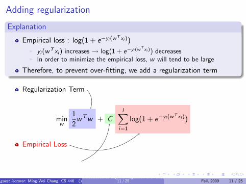
Explanation
Empirical loss : log(1 + e−yi (wT xi ))
I yi (wT xi ) increases → log(1 + e−yi (w
T xi )) decreasesI In order to minimize the empirical loss, w will tend to be large
Therefore, to prevent over-fitting, we add a regularization term
Regularization Term
minw
1
2wTw + C
l∑i=1
log(1 + e−yi (wT xi ))
Empirical Loss
balance parameter
guest lecturer: Ming-Wei Chang CS 446 ()Introduction to Logistic Regression and Support Vector Machine
11 / 25 Fall, 2009 11 / 25

Adding regularization
Explanation
Empirical loss : log(1 + e−yi (wT xi ))
I yi (wT xi ) increases → log(1 + e−yi (w
T xi )) decreasesI In order to minimize the empirical loss, w will tend to be large
Therefore, to prevent over-fitting, we add a regularization term
Regularization Term
minw
1
2wTw + C
l∑i=1
log(1 + e−yi (wT xi ))
Empirical Loss
balance parameter
guest lecturer: Ming-Wei Chang CS 446 ()Introduction to Logistic Regression and Support Vector Machine
11 / 25 Fall, 2009 11 / 25
Optimization
An unconstrained problem. We can use the gradient descentalgorithm!
However, it is quite slow.
Many other methodsIterative scaling; non-linear conjugate gradient; quasi-Newtonmethods; truncated Newton methods; trust-region newton method.
All methods are iterative methods, that generate a sequence wk
Converging to the optimal solution of the optimization problem above.
Choice of optimization techniques
Low cost per iteration – High cost per iteration(slow convergence) (fast convergence)Iterative scaling Newton Methods(each w component at a time)
Currently: Limited memory BFGS is very popular in NLP community
guest lecturer: Ming-Wei Chang CS 446 ()Introduction to Logistic Regression and Support Vector Machine
12 / 25 Fall, 2009 12 / 25

Optimization
An unconstrained problem. We can use the gradient descentalgorithm! However, it is quite slow.
Many other methods
Iterative scaling; non-linear conjugate gradient; quasi-Newtonmethods; truncated Newton methods; trust-region newton method.
All methods are iterative methods, that generate a sequence wk
Converging to the optimal solution of the optimization problem above.
Choice of optimization techniques
Low cost per iteration – High cost per iteration(slow convergence) (fast convergence)Iterative scaling Newton Methods(each w component at a time)
Currently: Limited memory BFGS is very popular in NLP community
guest lecturer: Ming-Wei Chang CS 446 ()Introduction to Logistic Regression and Support Vector Machine
12 / 25 Fall, 2009 12 / 25

Optimization
An unconstrained problem. We can use the gradient descentalgorithm! However, it is quite slow.
Many other methodsIterative scaling; non-linear conjugate gradient; quasi-Newtonmethods; truncated Newton methods; trust-region newton method.
All methods are iterative methods, that generate a sequence wk
Converging to the optimal solution of the optimization problem above.
Choice of optimization techniques
Low cost per iteration – High cost per iteration(slow convergence) (fast convergence)Iterative scaling Newton Methods(each w component at a time)
Currently: Limited memory BFGS is very popular in NLP community
guest lecturer: Ming-Wei Chang CS 446 ()Introduction to Logistic Regression and Support Vector Machine
12 / 25 Fall, 2009 12 / 25

Optimization
An unconstrained problem. We can use the gradient descentalgorithm! However, it is quite slow.
Many other methodsIterative scaling; non-linear conjugate gradient; quasi-Newtonmethods; truncated Newton methods; trust-region newton method.
All methods are iterative methods, that generate a sequence wk
Converging to the optimal solution of the optimization problem above.
Choice of optimization techniques
Low cost per iteration – High cost per iteration(slow convergence) (fast convergence)Iterative scaling Newton Methods(each w component at a time)
Currently: Limited memory BFGS is very popular in NLP community
guest lecturer: Ming-Wei Chang CS 446 ()Introduction to Logistic Regression and Support Vector Machine
12 / 25 Fall, 2009 12 / 25

Logistic regression versus Naive Bayes
Logistic regression Naive Bayes
Training maximize P(Y |X ) maximize P(Y ,X )
Training Algorithm optimization algorithms counting
Testing P(y |x) ≥ 0.5? P(y |x) ≥ 0.5?
Table: Comparison between Naive Bayes and logistic regression
LR and NB are both linear functions in the testing phase
However, their training agendas are very different
guest lecturer: Ming-Wei Chang CS 446 ()Introduction to Logistic Regression and Support Vector Machine
13 / 25 Fall, 2009 13 / 25

Support Vector Machine: another loss function
No magic. Just another loss function
Logistic Regression
minw
1
2wTw + C
l∑i=1
log(1 + e−yi (wT xi ))
L1-loss SVM
minw
1
2wTw + C
l∑i=1
max(0, 1− yiwT xi )
L2-loss SVM
minw
1
2wTw + C
l∑i=1
max(0, 1− yiwT xi )
2
guest lecturer: Ming-Wei Chang CS 446 ()Introduction to Logistic Regression and Support Vector Machine
14 / 25 Fall, 2009 14 / 25

Compare these loss functions
guest lecturer: Ming-Wei Chang CS 446 ()Introduction to Logistic Regression and Support Vector Machine
15 / 25 Fall, 2009 15 / 25

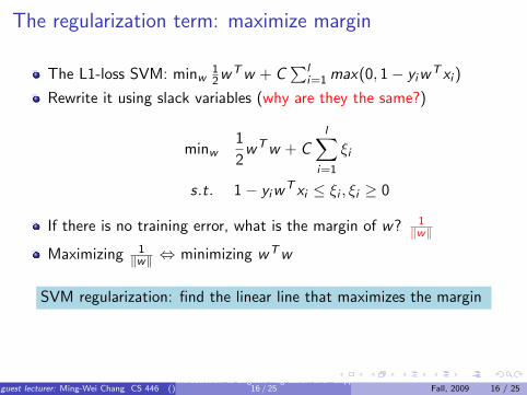
The regularization term: maximize margin
The L1-loss SVM: minw12wTw + C
∑li=1 max(0, 1− yiw
T xi )
Rewrite it using slack variables (why are they the same?)
minw1
2wTw + C
l∑i=1
ξi
s.t. 1− yiwT xi ≤ ξi , ξi ≥ 0
If there is no training error, what is the margin of w? 1‖w‖
Maximizing 1‖w‖ ⇔ minimizing wTw
SVM regularization: find the linear line that maximizes the margin
Learning theory: Link to SVM theory notes
guest lecturer: Ming-Wei Chang CS 446 ()Introduction to Logistic Regression and Support Vector Machine
16 / 25 Fall, 2009 16 / 25

The regularization term: maximize margin
The L1-loss SVM: minw12wTw + C
∑li=1 max(0, 1− yiw
T xi )
Rewrite it using slack variables (why are they the same?)
minw1
2wTw + C
l∑i=1
ξi
s.t. 1− yiwT xi ≤ ξi , ξi ≥ 0
If there is no training error, what is the margin of w?
1‖w‖
Maximizing 1‖w‖ ⇔ minimizing wTw
SVM regularization: find the linear line that maximizes the margin
Learning theory: Link to SVM theory notes
guest lecturer: Ming-Wei Chang CS 446 ()Introduction to Logistic Regression and Support Vector Machine
16 / 25 Fall, 2009 16 / 25

The regularization term: maximize margin
The L1-loss SVM: minw12wTw + C
∑li=1 max(0, 1− yiw
T xi )
Rewrite it using slack variables (why are they the same?)
minw1
2wTw + C
l∑i=1
ξi
s.t. 1− yiwT xi ≤ ξi , ξi ≥ 0
If there is no training error, what is the margin of w? 1‖w‖
Maximizing 1‖w‖ ⇔ minimizing wTw
SVM regularization: find the linear line that maximizes the margin
Learning theory: Link to SVM theory notes
guest lecturer: Ming-Wei Chang CS 446 ()Introduction to Logistic Regression and Support Vector Machine
16 / 25 Fall, 2009 16 / 25
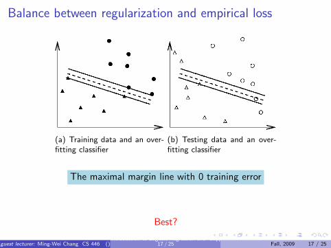
Balance between regularization and empirical loss
(a) Training data and an over-fitting classifier
(b) Testing data and an over-fitting classifier
The maximal margin line with 0 training error
Best?
guest lecturer: Ming-Wei Chang CS 446 ()Introduction to Logistic Regression and Support Vector Machine
17 / 25 Fall, 2009 17 / 25
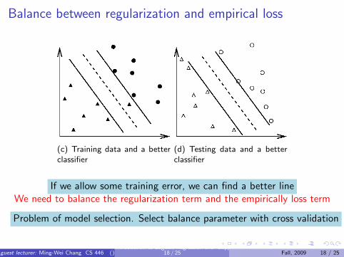
Balance between regularization and empirical loss
(c) Training data and a betterclassifier
(d) Testing data and a betterclassifier
If we allow some training error, we can find a better lineWe need to balance the regularization term and the empirically loss term
Problem of model selection. Select balance parameter with cross validation
guest lecturer: Ming-Wei Chang CS 446 ()Introduction to Logistic Regression and Support Vector Machine
18 / 25 Fall, 2009 18 / 25
Primal and Dual Formulations
Explaining the primal-dual relationship
Link to the lecture notes: 07-LecSvm-opt.pdf
Why primal-dual relationship is useful
Link to a talk by Professor Chih-Jen Lin in 2005.I Optimization, Support Vector Machines, and Machine Learning. Talk
in DIS, University of Rome and IASI, CNR, Italy. September 1-2, 2005.
We will only use the slides from page 11-20.
Link to notes
guest lecturer: Ming-Wei Chang CS 446 ()Introduction to Logistic Regression and Support Vector Machine
19 / 25 Fall, 2009 19 / 25

Nonlinear SVM
SVM tries to find a linear line that maximizes the margin.
Why people mention about non-linear SVM?
I Usually this means: x → φ(x)F Find a linear function of φ(x)F This can be a non linear function for x
Primal
minw ,ξi
1
2wTw + C
l∑i=1
ξi
s.t. 1− yiwTφ(x)i ≤ ξi
ξi ≥ 0,∀i = 1 . . . l
Dual
minα1
2αTQα− eTα
s.t. ∀i , 0 ≤ αi ≤ C
where Q is a l-by-l matrixwith Qij = yiyjK (xi , xj)
Same for Kernel perceptron: find a linear function on φ(x)
Demo
guest lecturer: Ming-Wei Chang CS 446 ()Introduction to Logistic Regression and Support Vector Machine
20 / 25 Fall, 2009 20 / 25

Nonlinear SVM
SVM tries to find a linear line that maximizes the margin.
Why people mention about non-linear SVM?I Usually this means: x → φ(x)
F Find a linear function of φ(x)F This can be a non linear function for x
Primal
minw ,ξi
1
2wTw + C
l∑i=1
ξi
s.t. 1− yiwTφ(x)i ≤ ξi
ξi ≥ 0,∀i = 1 . . . l
Dual
minα1
2αTQα− eTα
s.t. ∀i , 0 ≤ αi ≤ C
where Q is a l-by-l matrixwith Qij = yiyjK (xi , xj)
Same for Kernel perceptron: find a linear function on φ(x)
Demo
guest lecturer: Ming-Wei Chang CS 446 ()Introduction to Logistic Regression and Support Vector Machine
20 / 25 Fall, 2009 20 / 25

Solving SVM
Both primal and dual problems have constraintsI We can not use the gradient descent algorithm
For linear dual SVM, there is a simple optimization algorithmI Coordinate descent method!
minα1
2αTQα− eTα
s.t. ∀i , 0 ≤ αi ≤ C
I # of αi = # of training exampleI The idea: pick one example i . Optimize αi only
guest lecturer: Ming-Wei Chang CS 446 ()Introduction to Logistic Regression and Support Vector Machine
21 / 25 Fall, 2009 21 / 25
Coordinate Descent Algorithm
Algorithm
Run through the training data multiple times
I Pick a random example (i) among the training data.I Fix α1, α2, . . . , αi−1, αi+1, . . . , αl , only change αi
α′i = αi + s
I Solve the problem
mins1
2(α + sd)TQ(α + sd)− eT (α + sd)
s.t. 0 ≤ αi + s ≤ C ⇐ only one constraint,
where d is a vector of l − 1 zeros. The i-th component of d is 1.I It is a single variable problem. We know how to solve this.
guest lecturer: Ming-Wei Chang CS 446 ()Introduction to Logistic Regression and Support Vector Machine
22 / 25 Fall, 2009 22 / 25

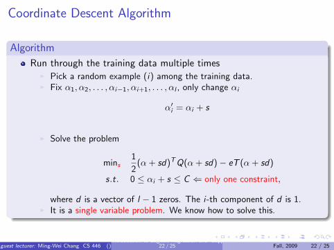
Coordinate Descent Algorithm
Algorithm
Run through the training data multiple timesI Pick a random example (i) among the training data.
I Fix α1, α2, . . . , αi−1, αi+1, . . . , αl , only change αi
α′i = αi + s
I Solve the problem
mins1
2(α + sd)TQ(α + sd)− eT (α + sd)
s.t. 0 ≤ αi + s ≤ C ⇐ only one constraint,
where d is a vector of l − 1 zeros. The i-th component of d is 1.I It is a single variable problem. We know how to solve this.
guest lecturer: Ming-Wei Chang CS 446 ()Introduction to Logistic Regression and Support Vector Machine
22 / 25 Fall, 2009 22 / 25

Coordinate Descent Algorithm
Algorithm
Run through the training data multiple timesI Pick a random example (i) among the training data.I Fix α1, α2, . . . , αi−1, αi+1, . . . , αl , only change αi
α′i = αi + s
I Solve the problem
mins1
2(α + sd)TQ(α + sd)− eT (α + sd)
s.t. 0 ≤ αi + s ≤ C ⇐ only one constraint,
where d is a vector of l − 1 zeros. The i-th component of d is 1.
I It is a single variable problem. We know how to solve this.
guest lecturer: Ming-Wei Chang CS 446 ()Introduction to Logistic Regression and Support Vector Machine
22 / 25 Fall, 2009 22 / 25
Coordinate Descent Algorithm
Algorithm
Run through the training data multiple timesI Pick a random example (i) among the training data.I Fix α1, α2, . . . , αi−1, αi+1, . . . , αl , only change αi
α′i = αi + s
I Solve the problem
mins1
2(α + sd)TQ(α + sd)− eT (α + sd)
s.t. 0 ≤ αi + s ≤ C ⇐ only one constraint,
where d is a vector of l − 1 zeros. The i-th component of d is 1.I It is a single variable problem. We know how to solve this.
guest lecturer: Ming-Wei Chang CS 446 ()Introduction to Logistic Regression and Support Vector Machine
22 / 25 Fall, 2009 22 / 25

Coordinate Descent Algorithm
Assume that the optimal s is s∗. We can update αi using:
α′i = αi + s∗
⇐ Similar to dual perceptron
Given that w =∑l
i αiyixi , this is equivalent to is equivalent to
w ← w + (α′i − αi )yixi
⇐ Similar to primal perceptron
Isn’t this familiar?
guest lecturer: Ming-Wei Chang CS 446 ()Introduction to Logistic Regression and Support Vector Machine
23 / 25 Fall, 2009 23 / 25
Coordinate Descent Algorithm
Assume that the optimal s is s∗. We can update αi using:
α′i = αi + s∗ ⇐ Similar to dual perceptron
Given that w =∑l
i αiyixi , this is equivalent to is equivalent to
w ← w + (α′i − αi )yixi
⇐ Similar to primal perceptron
Isn’t this familiar?
guest lecturer: Ming-Wei Chang CS 446 ()Introduction to Logistic Regression and Support Vector Machine
23 / 25 Fall, 2009 23 / 25

Coordinate Descent Algorithm
Assume that the optimal s is s∗. We can update αi using:
α′i = αi + s∗ ⇐ Similar to dual perceptron
Given that w =∑l
i αiyixi , this is equivalent to is equivalent to
w ← w + (α′i − αi )yixi ⇐ Similar to primal perceptron
Isn’t this familiar?
guest lecturer: Ming-Wei Chang CS 446 ()Introduction to Logistic Regression and Support Vector Machine
23 / 25 Fall, 2009 23 / 25

Relationships between linear classifiers
NB, LR, Perceptron and SVM are all linear classifiers
NB and LR have the same interpretation for conditional probability
P(y |x ,w) =1
1 + e−y(wT x)(2)
The difference between LR and SVM are their loss functionsI But they are quite similar!
Perceptron algorithm and the coordinate descent algorithm for SVMare very similar
guest lecturer: Ming-Wei Chang CS 446 ()Introduction to Logistic Regression and Support Vector Machine
24 / 25 Fall, 2009 24 / 25

Summary
Logistic regression
Maximizes P(Y |X ) while Naive Bayes maximizes the joint probabilityP(Y ,X )
Model the conditional probability using a linear line. Drop theconditional independence assumption
Many available methods of optimizing the objective function
Support Vector Machine
Similar to Logistic Regression; Different Loss function
Maximizes Margin; Has many nice theoretical properties
Interesting Primal-Dual relationshipI Allows us to choose the easier one to solve
Many available methods of optimizing the objective functionI The linear dual coordinate descent method turns out to be similar to
Perceptron
guest lecturer: Ming-Wei Chang CS 446 ()Introduction to Logistic Regression and Support Vector Machine
25 / 25 Fall, 2009 25 / 25