introduction to discrete-time signals and systems · welcome to discrete time signals and systems...
TRANSCRIPT

Introduction toDiscrete-Time Signals and Systems

Welcome to Discrete Time Signals and Systems
This is an introductory course on signal processing that studies signals and systems
Signal (n): A detectable physical quantity . . . by which messages or informationcan be transmitted (Merriam-Webster)
DE
FIN
ITIO
N
Signals carry information
Examples:
• Speech signals transmit language via acoustic waves• Radar signals transmit the position and velocity of targets via electromagnetic waves• Electrophysiology signals transmit information about processes inside the body• Financial signals transmit information about events in the economy
2

Welcome to Discrete Time Signals and Systems
Systems manipulate the information carried by signals
Signal processing involves the theory and application of
• filtering, coding, transmitting, estimating, detecting, analyzing, recognizing,
synthesizing, recording, and reproducing signals by digital or analog devices or
techniques
• where signal includes audio, video, speech, image, communication, geophysical,
sonar, radar, medical, musical, and other signals
(IEEE Signal Processing Society Constitutional Amendment, 1994)
DE
FIN
ITIO
N
3

Signal Processing
Signal processing has traditionally been a part of electrical and computer engineering
But now expands into applied mathematics, statistics, computer science, geophysics, and host ofapplication disciplines
Initially analog signals and systems implemented using resistors, capacitors, inductors, andtransistors
Since the 1940s increasingly digital signals and systems implemented using computers andcomputer code (Matlab, Python, C, . . . )
• Advantages of digital include stability and programmability• As computers have shrunk, digital signal processing has become ubiquitous
4

Digital Signal Processing Applications
5

Discrete Time Signals and Systems
This edX course consists of one-half of the coreElectrical and Computer Engineering course entitled“Signals and Systems” taught at Rice Universityin Houston, Texas, USA (see www.dsp.rice.edu)
Goals: Develop intuition into and learn how to reason analytically about signal processingproblems
Video lectures, primary sources, supplemental materials, practice exercises, homework,programming case studies, final exam
Integrated Matlab!
The course comes in two halves• Part 1: Time Domain• Part 2: Frequency Domain
6

Course Outline
Part 1: Time Domain
• Week 1: Types of Signals
• Week 2: Signals Are Vectors
• Week 3: Systems
• Week 4: Convolution
• Week 5: Study Week, Practice Exam, Final Exam
Part 2: Frequency Domain
• Week 1: Discrete Fourier Transform (DFT)
• Week 2: Discrete-Time Fourier Transform (DTFT)
• Week 3: z Transform
• Week 4: Analysis and Design of Discrete-Time Filters
• Week 5: Study Week, Practice Exam, Final Exam
7

What You Should Do Each Week
Watch the Lecture videos
Do the Exercises (on the page to the right of the videos)
As necessary, refer to the lesson’s Supplemental Resources (the page to the right of the exercises)
Do the homework problems
Some weeks will also have graded MATLAB case study homework problems
8

Logistics and GradingHow to get help: Course Discussion page
• Use a thread set up for a particular topic, or• Start a new thread
Rules for discussion
• Be respectful and helpful• Do not reveal answers to any problem that will be graded
Grading
Quick Questions 15%Homework 30%Homework Free Response Questions 15%Pre-Exam Survey 5%Final exam 30%Post-Exam Survey 5%
Passing grade: 60%
9

Supplemental Resources
After the video lecture and a practice exercise or two, you will often see additionalSupplemental Resources
Sometimes these will contain background material to provide motivation for the topic
Sometimes these will provide a refresher of pre-requisite concepts
Sometimes these will provide deeper explanations of the content (more rigorous proofs, etc.)
Sometimes a particular signal processing application will be showcased
Important: Though the content in these resources will not be assessed in the homework or exam,you may find that they help you to understand a concept better or increase your interest in it
10

Before You Start
Important: This is a mathematical treatment of signals and systems (no pain, no gain!)
Please make sure you have a solid understanding of
• Complex numbers and arithmetic
• Linear algebra (vectors, matrices, dot products, eigenvectors, bases . . . )
• Series (finite and infinite)
• Calculus of a single variable (derivatives and integrals)
• Matlab
To test your readiness or refresh your knowledge, visit the “Pre-class Mathematics Refresher”section of the course
11

Discrete Time Signals and Systems
12
Discrete Time Signals

Signals
Signal (n): A detectable physical quantity . . . by which messages or informationcan be transmitted (Merriam-Webster)
DEFINITIO
N
Signals carry information
Examples:
• Speech signals transmit language via acoustic waves• Radar signals transmit the position and velocity of targets via electromagnetic waves• Electrophysiology signals transmit information about processes inside the body• Financial signals transmit information about events in the economy
Signal processing systems manipulate the information carried by signals
This is a course about signals and systems
2

Signals are Functions
A signal is a function that maps an independent variable to a dependent variable.
DEFINITIO
N
Signal x[n]: each value of n produces the value x[n]
In this course, we will focus on discrete-time signals:
• Independent variable is an integer: n ∈ Z (will refer to as time)
• Dependent variable is a real or complex number: x[n] ∈ R or C
n
x[n]......
−1 0 1 2 3 4 5 6 7
3

Plotting Real Signals
When x[n] ∈ R (ex: temperature in a room at noon on Monday), we use one signal plot
−15 −10 −5 0 5 10 15−1
0
1
n
x[n]
When it is clear from context, we will often suppress the labels on one or both axes, like this
4
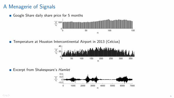
A Menagerie of Signals
Google Share daily share price for 5 months
0 50 100 1500
500
n
x[n]
Temperature at Houston Intercontinental Airport in 2013 (Celcius)
0 50 100 150 200 250 300 3500
20
40
n
x[n]
Excerpt from Shakespeare’s Hamlet
0 1000 2000 3000 4000 5000 6000 7000
−0.2
0
0.2
0.4
n
x[n]
5

Plotting Signals CorrectlyIn a discrete-time signal x[n], the independent variable n is discrete (integer)
To plot a discrete-time signal in a program like Matlab, you should use the stem or similarcommand and not the plot command
Correct:
−15 −10 −5 0 5 10 15−1
0
1
n
x[n]
Incorrect:
−15 −10 −5 0 5 10 15−1
0
1
n
x[n]
6

Plotting Complex Signals
Recall that a complex number a ∈ C can be equivalently represented two ways:
• Polar form: a = |a| ej∠a
• Rectangular form: a = Re{a}+ j Im{a}
Here j =√−1 (engineering notation; mathematicians use i =
√−1)
When x[n] ∈ C (ex: magnitude and phase of an electromagnetic wave), we use two signal plots
• Rectangular form: x[n] = Re{x[n]}+ j Im{x[n]}
• Polar form: x[n] = |x[n]| ej∠x[n]
7

Plotting Complex Signals (Rectangular Form)
Rectangular form: x[n] = Re{x[n]}+ j Im{x[n]} ∈ C
−15 −10 −5 0 5 10 15−1
0
1
n
Refx
[n]g
−15 −10 −5 0 5 10 15−2
−1
0
1
n
Imfx[n]g
8

Plotting Complex Signals (Polar Form)
Polar form: x[n] = |x[n]| ej∠(x[n]) ∈ C
−15 −10 −5 0 5 10 150
1
2
n
jx[n]j
−15 −10 −5 0 5 10 15−4−2024
n
\x[n]
9

Summary
Discrete-time signals
• Independent variable is an integer: n ∈ Z (will refer to as time)• Dependent variable is a real or complex number: x[n] ∈ R or C
Plot signals correctly!
10

Signal Properties

Signal Properties
Infinite/finite-length signals
Periodic signals
Causal signals
Even/odd signals
Digital signals
2

Finite/Infinite-Length SignalsAn infinite-length discrete-time signal x[n] is defined for all n ∈ Z, i.e., −∞ < n <∞
−15 −10 −5 0 5 10 15−1
0
1
nx[n] . . .
A finite-length discrete-time signal x[n] is defined only for a finite range of N1 ≤ n ≤ N2
−15 −10 −5 0 5 10 15−1
0
1
n
x[n]
Important: a finite-length signal is undefined for n < N1 and n > N2
3

Periodic Signals
A discrete-time signal is periodic if it repeats with period N ∈ Z:
x[n+mN ] = x[n] ∀m ∈ Z
DE
FIN
ITIO
N
−15 −10 −5 0 5 10 15 200
2
4
n
x[n]
Notes:
The period N must be an integer
A periodic signal is infinite in length
A discrete-time signal is aperiodic if it is not periodic
DE
FIN
ITIO
N
4

Converting between Finite and Infinite-Length Signals
Convert an infinite-length signal into a finite-length signal by windowing
Convert a finite-length signal into an infinite-length signal by either
• (infinite) zero padding, or
• periodization
5

Windowing
Converts a longer signal into a shorter one y[n] =
{x[n] N1 ≤ n ≤ N2
0 otherwise
−15 −10 −5 0 5 10 15−1
0
1
x[n]
n
6

Zero Padding
Converts a shorter signal into a longer one
Say x[n] is defined for N1 ≤ n ≤ N2
Given N0 ≤ N1 ≤ N2 ≤ N3 y[n] =
0 N0 ≤ n < N1
x[n] N1 ≤ n ≤ N2
0 N2 < n ≤ N3
−15 −10 −5 0 5 10 15−1
0
1
x[n]
n
7

PeriodizationConverts a finite-length signal into an infinite-length, periodic signal
Given finite-length x[n], replicate x[n] periodically with period N
y[n] =
∞∑m=−∞
x[n−mN ], n ∈ Z
= · · ·+ x[n+ 2N ] + x[n+N ] + x[n] + x[n−N ] + x[n− 2N ] + · · ·
0 1 2 3 4 5 6 70
2
4
x[n]
n
−15 −10 −5 0 5 10 15 200
2
4
y [n ] with period N = 8
n
8
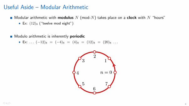
Useful Aside – Modular Arithmetic
Modular arithmetic with modulus N (mod-N) takes place on a clock with N “hours”
• Ex: (12)8 (“twelve mod eight”)
Modulo arithmetic is inherently periodic
• Ex: . . . (−12)8 = (−4)8 = (4)8 = (12)8 = (20)8 . . .
9

Periodization via Modular Arithmetic
Consider a length-N signal x[n] defined for 0 ≤ n ≤ N − 1
A convenient way to express periodization with period N is y[n] = x[(n)N ], n ∈ Z
0 1 2 3 4 5 6 70
2
4
x[n]
n
−15 −10 −5 0 5 10 15 200
2
4
y [n ] with period N = 8
n
Important interpretation
• Infinite-length signals live on
the (infinite) number line• Periodic signals live on a circle
– a clock with N “hours”
10

Finite-Length and Periodic Signals are Equivalent
0 1 2 3 4 5 6 70
2
4
x[n]
n
−15 −10 −5 0 5 10 15 200
2
4
y [n ] with period N = 8
n
All of the information in a periodic signal is contained in one period (of finite length)
Any finite-length signal can be periodized
Conclusion: We can and will think of finite-length signals and periodic signals interchangeably
We can choose the most convenient viewpoint for solving any given problem
• Application: Shifting finite length signals
11

Causal Signals
A signal x[n] is causal if x[n] = 0 for all n < 0.
DE
FIN
ITIO
N
−10 −5 0 5 10 150
0.5
1
n
x[n]
A signal x[n] is anti-causal if x[n] = 0 for all n ≥ 0
−10 −5 0 5 10 150
0.5
1
n
x[n]
A signal x[n] is acausal if it is not causal
12

Even Signals
A real signal x[n] is even if x[−n] = x[n]
DE
FIN
ITIO
N
−15 −10 −5 0 5 10 150
0.5
1
x[n]
n
Even signals are symmetrical around the point n = 0
13

Odd Signals
A real signal x[n] is odd if x[−n] = −x[n]
DE
FIN
ITIO
N
−15 −10 −5 0 5 10 15−0.5
0
0.5
n
x[n]
Odd signals are anti-symmetrical around the point n = 0
14

Even+Odd Signal Decomposition
Useful fact: Every signal x[n] can be decomposed into the sum of its even part + its odd part
Even part: e[n] = 12 (x[n] + x[−n]) (easy to verify that e[n] is even)
Odd part: o[n] = 12 (x[n]− x[−n]) (easy to verify that o[n] is odd)
Decomposition x[n] = e[n] + o[n]
Verify the decomposition:
e[n] + o[n] =1
2(x[n] + x[−n]) + 1
2(x[n]− x[−n])
=1
2(x[n] + x[−n] + x[n]− x[−n])
=1
2(2x[n]) = x[n] X
15

Even+Odd Signal Decomposition in Pictures
−15 −10 −5 0 5 10 150
0.5
1
x[n ]
n
16

Even+Odd Signal Decomposition in Pictures
12
−15 −10 −5 0 5 10 150
0.5
1
x[n]
n
+−15 −10 −5 0 5 10 150
0.5
1
x[−n]
n
=−15 −10 −5 0 5 10 150
0.5
1
e[n]
n
+
12
−15 −10 −5 0 5 10 150
0.5
1
x[n]
n
−−15 −10 −5 0 5 10 150
0.5
1
x[−n]
n
=−15 −10 −5 0 5 10 15
−0.5
0
0.5
o[n]
n
=
−15 −10 −5 0 5 10 150
0.5
1
x[n]
n
17

Digital Signals
Digital signals are a special sub-class of discrete-time signals
• Independent variable is still an integer: n ∈ Z
• Dependent variable is from a finite set of integers: x[n] ∈ {0, 1, . . . , D − 1}
• Typically, choose D = 2q and represent each possible level of x[n] as a digital code with q bits
• Ex: Digital signal with q = 2 bits ⇒ D = 22 = 4 levels
−15 −10 −5 0 5 10 150
1
2
3
n
Q(x
[n])
• Ex: Compact discs use q = 16 bits ⇒ D = 216 = 65536 levels
18

Summary
Signals can be classified many different ways (real/complex, infinite/finite-length,periodic/aperiodic, causal/acausal, even/odd, . . . )
Finite-length signals are equivalent to periodic signals; modulo arithmetic useful
19

Shifting Signals

Shifting Infinite-Length SignalsGiven an infinite-length signal x[n], we can shift it back and forth in time via x[n−m], m ∈ Z
0 10 20 30 40 50 60−1
0
1
x[n]
n
When m > 0, x[n−m] shifts to the right (forward in time, delay)
0 10 20 30 40 50 60−1
0
1
x[n− 10]
n
When m < 0, x[n−m] shifts to the left (back in time, advance)
0 10 20 30 40 50 60−1
0
1
x[n+ 10]
n
2
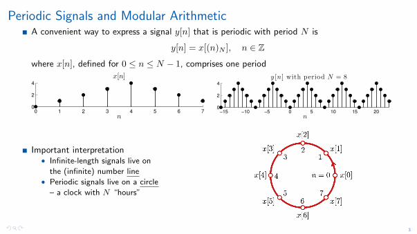
Periodic Signals and Modular ArithmeticA convenient way to express a signal y[n] that is periodic with period N is
y[n] = x[(n)N ], n ∈ Z
where x[n], defined for 0 ≤ n ≤ N − 1, comprises one period
0 1 2 3 4 5 6 70
2
4
x[n]
n
−15 −10 −5 0 5 10 15 200
2
4
y [n ] with period N = 8
n
Important interpretation• Infinite-length signals live on
the (infinite) number line• Periodic signals live on a circle
– a clock with N “hours”
3

Shifting Periodic Signals
Periodic signals can also be shifted; consider y[n] = x[(n)N ]
−15 −10 −5 0 5 10 15 200
2
4
y[n] with period N = 8
n
Shift one sample into the future: y[n− 1] = x[(n− 1)N ]
−15 −10 −5 0 5 10 15 200
2
4
y[n− 1] with period N = 8
n
4

Shifting Finite-Length Signals
Consider finite-length signals x and v defined for 0 ≤ n ≤ N − 1 and suppose “v[n] = x[n− 1]”
v[0] = ??
v[1] = x[0]
v[2] = x[1]
v[3] = x[2]
...
v[N − 1] = x[N − 2]
?? = x[N − 1]
What to put in v[0]? What to do with x[N − 1]? We don’t want to invent/lose information
Elegant solution: Assume x and v are both periodic with period N ; then v[n] = x[(n− 1)N ]
This is called a periodic or circular shift (see circshift and mod in Matlab)
5
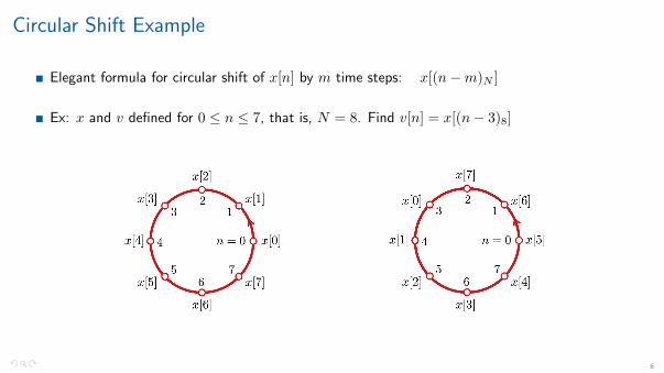
Circular Shift Example
Elegant formula for circular shift of x[n] by m time steps: x[(n−m)N ]
Ex: x and v defined for 0 ≤ n ≤ 7, that is, N = 8. Find v[n] = x[(n− 3)8]
6

Circular Shift Example
Elegant formula for circular shift of x[n] by m time steps: x[(n−m)N ]
Ex: x and v defined for 0 ≤ n ≤ 7, that is, N = 8. Find v[n] = x[(n−m)N ]
v[0] = x[5]
v[1] = x[6]
v[2] = x[7]
v[3] = x[0]
v[4] = x[1]
v[5] = x[2]
v[6] = x[3]
v[7] = x[4]
7

Circular Time Reversal
For infinite length signals, the transformation of reversing the time axis x[−n] is obvious
Not so obvious for periodic/finite-length signals
Elegant formula for reversing the time axis of a periodic/finite-length signal: x[(−n)N ]
Ex: x and v defined for 0 ≤ n ≤ 7, that is, N = 8. Find v[n] = x[(−n)N ]
v[0] = x[0]
v[1] = x[7]
v[2] = x[6]
v[3] = x[5]
v[4] = x[4]
v[5] = x[3]
v[6] = x[2]
v[7] = x[1]
8

Summary
Shifting a signal moves it forward or backward in time
Modulo arithmetic provides and easy way to shift periodic signals
9

Key Test Signals

A Toolbox of Test Signals
Delta function
Unit step
Unit pulse
Real exponential
Still to come: sinusoids, complex exponentials
Note: We will introduce the test signals as infinite-length signals,but each has a finite-length equivalent
2

Delta Function
The delta function (aka unit impulse) δ[n] =
{1 n = 0
0 otherwise
DE
FIN
ITIO
N
−15 −10 −5 0 5 10 150
0.5
1
n
[n]
±
The shifted delta function δ[n−m] peaks up at n = m; here m = 9
−15 −10 −5 0 5 10 150
0.5
1
n
[n¡9]
±
3
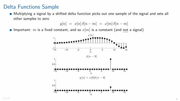
Delta Functions SampleMultiplying a signal by a shifted delta function picks out one sample of the signal and sets allother samples to zero
y[n] = x[n] δ[n−m] = x[m] δ[n−m]
Important: m is a fixed constant, and so x[m] is a constant (and not a signal)
−15 −10 −5 0 5 10 15−1
0
1
x[n ]
n
−15 −10 −5 0 5 10 150
0.5
1[n ¡ 9]
n
±
−15 −10 −5 0 5 10 150
0.5
1y [n ] = x[9]± [n ¡ 9]
n
4

Unit Step
The unit step u[n] =
{1 n ≥ 0
0 n < 0
DE
FIN
ITIO
N
−15 −10 −5 0 5 10 150
0.5
1
n
u[n
]
The shifted unit step u[n−m] jumps from 0 to 1 at n = m; here m = 5
−15 −10 −5 0 5 10 150
0.5
1
n
u[n¡5]
5
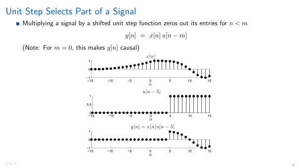
Unit Step Selects Part of a SignalMultiplying a signal by a shifted unit step function zeros out its entries for n < m
y[n] = x[n]u[n−m]
(Note: For m = 0, this makes y[n] causal)
−15 −10 −5 0 5 10 15−1
0
1
x[n ]
n
−15 −10 −5 0 5 10 150
0.5
1u[n ¡ 5]
n
−15 −10 −5 0 5 10 15−1
0
1y [n ] = x[n ]u[n ¡ 5]
n
6

Unit Pulse
The unit pulse (aka boxcar) p[n] =
0 n < N1
1 N1 ≤ n ≤ N2
0 n > N2DE
FIN
ITIO
N
Ex: p[n] for N1 = −5 and N2 = 3
−15 −10 −5 0 5 10 150
0.5
1
n
p[n
]
One of many different formulas for the unit pulse
p[n] = u[n−N1]− u[n− (N2 + 1)]
7

Real Exponential
The real exponential r[n] = an, a ∈ R, a ≥ 0
DE
FIN
ITIO
N
For a > 1, r[n] shrinks to the left and grows to the right; here a = 1.1
−15 −10 −5 0 5 10 150
2
4
n
r[n
]
For 0 < a < 1, r[n] grows to the left and shrinks to the right; here a = 0.9
−15 −10 −5 0 5 10 150
5
n
r[n
]
8

Summary
We will use our test signals often, especially the delta function and unit step
9

Sinusoids

Sinusoids
Sinusoids appear in myriad disciplines, in particular signal processing
They are the basis (literally) of Fourier analysis (DFT, DTFT)
We will introduce
• Real-valued sinusoids
• (Complex) sinusoid
• Complex exponential
2

SinusoidsThere are two natural real-valued sinusoids: cos(ωn+ φ) and sin(ωn+ φ)
Frequency: ω (units: radians/sample)Phase: φ (units: radians)
cos(ωn) (even)
−15 −10 −5 0 5 10 15−1
0
1
n
cos[!n]
sin(ωn) (odd)
−15 −10 −5 0 5 10 15−1
0
1
n
sin[wn]
3

Sinusoid Examples
cos(0n)
−15 −10 −5 0 5 10 150
0.5
1
n
sin(0n)
−15 −10 −5 0 5 10 15−1
0
1
n
sin(π4n+ 2π6 )
−15 −10 −5 0 5 10 15−1
0
1
n
cos(πn)
−15 −10 −5 0 5 10 15−1
0
1
n
4

Get Comfortable with Sinusoids!It’s easy to play around in Matlab to get comfortable with the properties of sinusoids
N=36;n=0:N-1;omega=pi/6;phi=pi/4;x=cos(omega*n+phi);stem(n,x)
0 5 10 15 20 25 30 35−1
−0.8
−0.6
−0.4
−0.2
0
0.2
0.4
0.6
0.8
1
5

Complex Sinusoid
The complex-valued sinusoid combines both the cos and sin terms (via Euler’s identity)
ej(ωn+φ) = cos(ωn+ φ) + j sin(ωn+ φ)
−15 −10 −5 0 5 10 150
0.5
1
jej!nj = 1
n−15 −10 −5 0 5 10 15−1
0
1
Re(ej!n) = cos(!n)
n
−15 −10 −5 0 5 10 15
−10
0
10
ej!n= !n
n
\
−15 −10 −5 0 5 10 15−1
0
1
Im(ej!n) = sin(!n)
n
6

A Complex Sinusoid is a Helix
ej(ωn+φ) = cos(ωn+ φ) + j sin(ωn+ φ)
A complex sinusoid is a helix in 3D space (Re{}, Im{}, n)• Real part (cos term) is the projection onto the Re{} axis• Imaginary part (sin term) is the projection onto the Im{} axis
Frequency ω determines rotation speed and direction of helix
• ω > 0 ⇒ anticlockwise rotation• ω < 0 ⇒ clockwise rotation
7

Complex Sinusoid is a Helix (Animation)
Complex sinusoid animation
8

Negative Frequency
Negative frequency is nothing to be afraid of! Consider a sinusoid with a negative frequency −ω
ej(−ω)n = e−jωn = cos(−ωn) + j sin(−ωn) = cos(ωn)− j sin(ωn)
Also note: ej(−ω)n = e−jωn =(ejωn
)∗Bottom line: negating the frequency is equivalent to complex conjugating a complex sinusoid,which flips the sign of the imaginary, sin term
−15 −10 −5 0 5 10 15−1
0
1
Re(ej!n) = cos(!n)
n−15 −10 −5 0 5 10 15−1
0
1
Re(e¡j!n) = cos(!n)
n
−15 −10 −5 0 5 10 15−1
0
1
Im(ej!n) = sin(!n)
n−15 −10 −5 0 5 10 15−1
0
1
Im(e¡ j!n) = ¡ sin(!n)
n
9

Phase of a Sinusoid ej(ωn+φ)
φ is a (frequency independent) shift that is referenced to one period of oscillation
cos(π6n− 0
)−15 −10 −5 0 5 10 15
−1
0
1
n
cos(π6n−
π4
)−15 −10 −5 0 5 10 15
−1
0
1
n
cos(π6n−
π2
)= sin
(π6n
)−15 −10 −5 0 5 10 15
−1
0
1
n
cos(π6n− 2π
)= cos
(π6n
)−15 −10 −5 0 5 10 15
−1
0
1
n10

Summary
Sinusoids play a starring role in both the theory and applications of signals and systems
A sinusoid has a frequency and a phase
A complex sinusoid is a helix in three-dimensional space and naturally induces the sine and cosine
Negative frequency is nothing to be scared by; it just means that the helix spins backwards
11

Discrete-Time Sinusoids Are Weird
Discrete-Time Sinusoids are Weird!
Discrete-time sinusoids ej(ωn+φ) have two counterintuitive properties
Both involve the frequency ω
Weird property #1: Aliasing
Weird property #2: Aperiodicity
2

Weird Property #1: Aliasing of Sinusoids
Consider two sinusoids with two different frequencies
• ω ⇒ x1[n] = ej(ωn+φ)
• ω + 2π ⇒ x2[n] = ej((ω+2π)n+φ)
But note that
x2[n] = ej((ω+2π)n+φ) = ej(ωn+φ)+j2πn = ej(ωn+φ) ej2πn = ej(ωn+φ) = x1[n]
The signals x1 and x2 have different frequencies but are identical!
We say that x1 and x2 are aliases; this phenomenon is called aliasing
Note: Any integer multiple of 2π will do; try with x3[n] = ej((ω+2πm)n+φ), m ∈ Z
3

Aliasing of Sinusoids – Example
x1[n] = cos(π6n
)
−15 −10 −5 0 5 10 15−1
0
1
n
x2[n] = cos(13π6 n
)= cos
((π6 + 2π)n
)
−15 −10 −5 0 5 10 15−1
0
1
n
4

Alias-Free Frequencies
Since
x3[n] = ej(ω+2πm)n+φ) = ej(ωn+φ) = x1[n] ∀m ∈ Z
the only frequencies that lead to unique (distinct) sinusoids lie in an interval of length 2π
Convenient to interpret the frequency ω as an angle(then aliasing is handled automatically; more on this later)
Two intervals are typically used in the signal processingliterature (and in this course)
• 0 ≤ ω < 2π
• −π < ω ≤ π
5

Low and High Frequencies
ej(ωn+φ)
Low frequencies: ω close to 0 or 2π radEx: cos
(π10n
)
−15 −10 −5 0 5 10 15−1
0
1
n
High frequencies: ω close to π or −π radEx: cos
(9π10n
)
−15 −10 −5 0 5 10 15−1
0
1
n
6
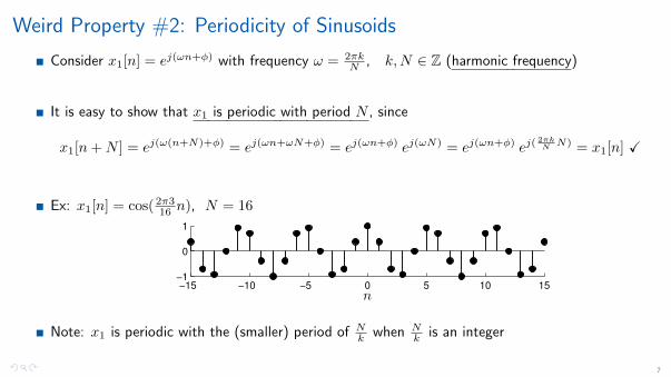
Weird Property #2: Periodicity of Sinusoids
Consider x1[n] = ej(ωn+φ) with frequency ω = 2πkN , k,N ∈ Z (harmonic frequency)
It is easy to show that x1 is periodic with period N , since
x1[n+N ] = ej(ω(n+N)+φ) = ej(ωn+ωN+φ) = ej(ωn+φ) ej(ωN) = ej(ωn+φ) ej(2πkN N) = x1[n] X
Ex: x1[n] = cos( 2π316 n), N = 16
−15 −10 −5 0 5 10 15−1
0
1
n
Note: x1 is periodic with the (smaller) period of Nk when N
k is an integer
7
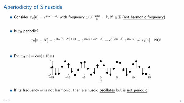
Aperiodicity of Sinusoids
Consider x2[n] = ej(ωn+φ) with frequency ω 6= 2πkN , k,N ∈ Z (not harmonic frequency)
Is x2 periodic?
x2[n+N ] = ej(ω(n+N)+φ) = ej(ωn+ωN+φ) = ej(ωn+φ) ej(ωN) 6= x1[n] NO!
Ex: x2[n] = cos(1.16n)
−15 −10 −5 0 5 10 15−1
0
1
n
If its frequency ω is not harmonic, then a sinusoid oscillates but is not periodic!
8

Harmonic Sinusoids
ej(ωn+φ)
Semi-amazing fact: The only periodic discrete-time sinusoids are those withharmonic frequencies
ω =2πk
N, k,N ∈ Z
Which means that
• Most discrete-time sinusoids are not periodic!
• The harmonic sinusoids are somehow magical (they play a starring role later in the DFT)
9

Harmonic Sinusoids (Matlab)
Click here to view a MATLAB demo that visualizes harmonic sinusoids.
10

Summary
Discrete-time sinusoids ej(ωn+φ) have two counterintuitive properties
Both involve the frequency ω
Weird property #1: Aliasing
Weird property #2: Aperidiocity
The only sinusoids that are periodic: Harmonic sinusoids ej(2πkN n+φ), n, k,N ∈ Z
11

Complex Exponentials

Complex Exponential
Complex sinusoid ej(ωn+φ) is of the form ePurely Imaginary Numbers
Generalize to eGeneral Complex Numbers
Consider the general complex number z = |z| ejω, z ∈ C
• |z| = magnitude of z• ω = ∠(z), phase angle of z• Can visualize z ∈ C as a point in the complex plane
Now we havezn = (|z|ejω)n = |z|n(ejω)n = |z|nejωn
• |z|n is a real exponential (an with a = |z|)• ejωn is a complex sinusoid
2

Complex Exponential is a Spiral
zn =(|z| ejω
)n= |z|n ejωn
|z|n is a real exponential envelope (an with a = |z|)
ejωn is a complex sinusoid
zn is a helix with expanding radius (spiral)
3

Complex Exponential is a Spiral
zn =(|z| ejωn
)n= |z|n ejωn
|z|n is a real exponential envelope (an with a = |z|)
ejωn is a complex sinusoid
|z| < 1 |z| > 1
−15 −10 −5 0 5 10 15−4−2024
Re(zn), |z|< 1
n−15 −10 −5 0 5 10 15−4
−2
0
2
Re(zn), jz j > 1
n
−15 −10 −5 0 5 10 15
−2024
Im(zn), |z|< 1
n−15 −10 −5 0 5 10 15−4
−2
0
2
Im(zn), |z|> 1
n
4

Complex Exponentials and z Plane (Matlab)
Click here to view a MATLAB demo plotting the signals zn.
5

Summary
Complex sinusoid ej(ωn+φ) is of the form ePurely Imaginary Numbers
Complex exponential: Generalize ej(ωn+φ) to eGeneral Complex Numbers
A complex exponential is the product of a real exponential and a complex sinusoid
A complex exponential is a spiral in three-dimensional space
6